Support Vector Machine Ensemble Based on Feature and...

Estefhan Dazzi Wandekokem

Support Vector Machine Ensemble Based onFeature and Hyperparameter Variation

Vitória - ES, Brasil

23 de fevereiro de 2011

Estefhan Dazzi Wandekokem

Support Vector Machine Ensemble Based onFeature and Hyperparameter Variation

Dissertação apresentada para obtenção do Graude Mestre em Informática pela UniversidadeFederal do Espírito Santo.

Orientador:

Dr. Thomas W. Rauber

Co-orientador:

Dr. Flávio M. Varejão

DEPARTAMENTO DE INFORMÁTICA

CENTRO TECNOLÓGICO

UNIVERSIDADE FEDERAL DO ESPÍRITOSANTO

Vitória - ES, Brasil

23 de fevereiro de 2011

Dissertação de Mestrado sob o título“Support Vector Machine Ensemble Based on

Feature and Hyperparameter Variation”, defendida por Estefhan Dazzi Wandekokem e aprovada

em 23 de fevereiro de 2011, em Vitória, Estado do Espírito Santo, pela banca examinadora con-

stituída pelos professores:

Dr. Thomas W. RauberOrientador

Dr. Flávio M. VarejãoCo-orientador

Dr. Renato KrohlingUniversidade Federal do Espírito Santo

Dr. Roberto M. Cesar, Jr.Universidade de São Paulo

Resumo

Classificadores do tipo máquina de vetores de suporte (SVM) são atualmente consideradosuma das técnicas mais poderosas para se resolver problemas de classificação com duas classes.Para aumentar o desempenho alcançado por classificadores SVM individuais, uma abordagembem estabelecida é usar uma combinação de SVMs, a qual corresponde a um conjunto de clas-sificadores SVMs que são, simultaneamente, individualmente precisos e coletivamente diver-gentes em suas decisões. Este trabalho propõe uma abordagempara se criar combinações deSVMs, baseada em um processo de três estágios. Inicialmente, são usadas execuções comple-mentares de uma busca baseada em algoritmos genéticos (GEFS), com o objetivo de investigarglobalmente o espaço de características para definir um conjunto de subconjuntos de caracterís-ticas. Em seguida, para cada um desses subconjuntos de características definidos, uma SVMque usa parâmetros otimizados é construída. Por fim, é empregada uma busca local com oobjetivo de selecionar um subconjunto otimizado dessas SVMs, e assim formar a combinaçãode SVMs que é finalmente produzida. Os experimentos foram realizados num contexto de de-tecção de defeitos em máquinas industriais. Foram usados 2000 exemplos de sinais de vibraçãode moto bombas instaladas em plataformas de petróleo. Os experimentos realizados mostramque o método proposto para se criar combinação de SVMs apresentou um desempenho superiorem comparação a outras abordagens de classificação bem estabelecidas.

Abstract

The support vector machine (SVM) classifier is currently considered one of the most pow-erful pattern recognition based techniques for solving binary classification problems. To furtherincrease the accuracy of an individual SVM, a well-established approach relies on using a SVMensemble, which is a set of accurate, divergent SVMs. In thiswork we investigate composingan ensemble with SVMs that differ among themselves on the feature subset and also the hy-perparameter value they use. We propose a three-stage method for building an SVM ensemble.First we use complementary Genetic Ensemble Feature Selection (GEFS) searches to globallyinvestigate the feature space, aiming to produce a set of diverse feature subsets. Further, foreach produced feature subset we build a SVM with tuned hyperparameters. Finally, we employa local search to retain an optimized, reduced set of these SVMs to ultimately comprise theensemble. Our experiments were performed in a context of real-world industrial machine faultdiagnosis. We use 2000 examples of vibration signals obtained from motor pumps installedon oil platforms. The performed experiments show that the proposed SVM ensemble methodachieved superior results in comparison to other well-established classification approaches.

Agradecimentos

Meus sinceros agradecimentos a todos os que colaboraram, direta ou indiretamente, à real-

ização deste trabalho.

À Petrobrás S.A. pelo apoio financeiro e pela disponibilização da base de dados utilizada.

À CAPES, pelo apoio financeiro.

Aos meus orientadores Thomas Rauber e Flávio Varejão, cujo conhecimento e entusiasmo

foram fundamentais para o sucesso deste trabalho.

Aos professores Roberto Cesar e Renato Krohling, membros da Banca Examinadora, que

gentilmente aceitaram dispor de seu tempo e conhecimento.

Aos colegas do laboratório NINFA, em especial Mendel, Fábioe Marcelo, pelas con-

tribuições, ajudas, conselhos e amizade. Também, aos meus amigos em geral, da engenharia e

de fora dela.

À minha família, pelo amor e apoio.

À Adriana, pelo amor e melhor companhia.

Contents

List of Figures

List of Tables

1 Introduction p. 12

1.1 Introduction . . . . . . . . . . . . . . . . . . . . . . . . . . . . . . . . . . . p. 13

1.2 Structure of this Work . . . . . . . . . . . . . . . . . . . . . . . . . . . . .. p. 14

2 Classifier Ensembles p. 15

2.1 Ensemble of Classifiers . . . . . . . . . . . . . . . . . . . . . . . . . . . . .p. 16

2.2 Combining Decisions from Distinct Classifiers . . . . . . . . . .. . . . . . p. 16

2.3 Generating Divergent Classifiers . . . . . . . . . . . . . . . . . . . .. . . . p. 18

3 Support Vector Machine Ensembles p. 20

3.1 The Support Vector Machine Classifier . . . . . . . . . . . . . . . . .. . . . p. 21

3.2 Previous Work on Support Vector Machine Ensemble

Methods . . . . . . . . . . . . . . . . . . . . . . . . . . . . . . . . . . . . . p. 22

4 SVM Ensemble Based on Feature and Hyperparameter Variation p. 24

4.1 Three-stage Approach to Build SVM Ensemble . . . . . . . . . . . .. . . . p. 25

4.2 First stage: Feature Variation . . . . . . . . . . . . . . . . . . . . .. . . . . p. 25

4.2.1 The GEFS Method . . . . . . . . . . . . . . . . . . . . . . . . . . . p. 27

4.2.2 The Multiple-GEFS Approach . . . . . . . . . . . . . . . . . . . . . p. 28

4.3 Second Stage: Hyperparameter Variation . . . . . . . . . . . . .. . . . . . . p. 29

4.4 Third Stage: Selection of the Final Ensemble . . . . . . . . . .. . . . . . . p. 29

5 Oil Rig Motor Pump Fault Diagnosis p. 31

5.1 Model-free Fault Diagnosis . . . . . . . . . . . . . . . . . . . . . . . .. . . p. 32

5.2 Motor Pump Equipment . . . . . . . . . . . . . . . . . . . . . . . . . . . . p.32

5.3 Considered Fault Categories . . . . . . . . . . . . . . . . . . . . . . . . .. p. 32

5.4 Extracted Features . . . . . . . . . . . . . . . . . . . . . . . . . . . . . . .p. 34

5.4.1 Fourier Spectrum Features . . . . . . . . . . . . . . . . . . . . . . .p. 35

5.4.2 Envelope Spectrum Features . . . . . . . . . . . . . . . . . . . . . .p. 36

6 Experimental Results p. 37

6.1 Cross-validation 5×2 . . . . . . . . . . . . . . . . . . . . . . . . . . . . . . p. 38

6.2 Studied Classification Models . . . . . . . . . . . . . . . . . . . . . . .. . p. 38

6.2.1 TheSVM Classification Model . . . . . . . . . . . . . . . . . . . . . p. 38

6.2.2 TheGEFS Classification Model . . . . . . . . . . . . . . . . . . . . p. 38

6.2.3 TheGEFS-Tuned Classification Model . . . . . . . . . . . . . . . p. 39

6.2.4 TheMultiple-GEFS Classification Model . . . . . . . . . . . . . p. 39

6.3 Cross-validation 5×2 Estimated Results . . . . . . . . . . . . . . . . . . . . p. 40

6.4 Influence of the Number of Evolved Generations and the Number of Compo-

nent SVMs . . . . . . . . . . . . . . . . . . . . . . . . . . . . . . . . . . . p. 41

6.4.1 Influence of the Number of Evolved Generations . . . . . . .. . . . p. 41

6.4.2 Influence of the Number of Component SVMs . . . . . . . . . . . . p. 42

6.5 Usefulness of Hyperparameter Tuning to Improve SVM Diversity . . . . . . p. 44

7 Conclusions and Future Work p. 51

7.1 Conclusions . . . . . . . . . . . . . . . . . . . . . . . . . . . . . . . . . . . p. 52

7.2 Future Work . . . . . . . . . . . . . . . . . . . . . . . . . . . . . . . . . . . p. 52

7.2.1 Using Data from Different Sources . . . . . . . . . . . . . . . . .. p. 52

7.2.2 Using Particle Swarm Optimization to Tune Hyperparameters . . . . p. 53

Bibliography p. 54

Appendix A -- Attached reference p. 57

List of Figures

2.1 The region of wrong decision of an ensemble (the shaded area) is smaller

than the region of wrong decision of any individual component classifiers

(the regionsR1, R2 andR3). . . . . . . . . . . . . . . . . . . . . . . . . . . p. 17

4.1 Construction of an ensembleE by the proposed Multiple-GEFS ensemble

method. . . . . . . . . . . . . . . . . . . . . . . . . . . . . . . . . . . . . . p. 26

5.1 Motor pump with accelerometers placed along the horizontal (H), axial (A)

and vertical (V) directions. The motor corresponds to positions the 1 and 2,

and the pump to the positions 3 and 4. . . . . . . . . . . . . . . . . . . . . .p. 33

5.2 Vibration signal Fourier spectrum of a motor pump presenting misalignment

and also an emerging hydrodynamic fault. . . . . . . . . . . . . . . . .. . . p. 34

6.1 AUC on test data achieved by each evolved generation of the GEFS method,

for the misalignment predictor. . . . . . . . . . . . . . . . . . . . . . . .. . p. 42


for the bearing - pump fault predictor. . . . . . . . . . . . . . . . . . .. . . p. 43


for the bearing - motor fault predictor. . . . . . . . . . . . . . . . . .. . . . p. 43

6.4 AUC on training and testing data achieved by each number of component

SVMs, during the classifier selection stage of the multiple-GEFS method, for

the misalignment predictor. . . . . . . . . . . . . . . . . . . . . . . . . . .. p. 44



the structural looseness - pump predictor. . . . . . . . . . . . . . .. . . . . p. 45



the structural looseness - motor predictor. . . . . . . . . . . . . .. . . . . . p. 45

6.7 AUC on test data achieved by the Multiple-GEFS method, and by individual

SVMs which use selected feature subsets with tuned or non-tuned hyperpara-

menters, for the misalignment predictor. . . . . . . . . . . . . . . .. . . . . p. 47



menters, for the structural looseness - pump predictor. . . .. . . . . . . . . . p. 48



menters, for the structural looseness - motor predictor. . .. . . . . . . . . . . p. 49



menters, for the mechanical looseness - pump predictor. . . .. . . . . . . . . p. 49



menters, for the mechanical looseness - motor predictor. . .. . . . . . . . . p. 50

List of Tables

5.1 Fault occurrence. . . . . . . . . . . . . . . . . . . . . . . . . . . . . . . . .p. 34

6.1 Test data AUC estimated by 5×2 cross-validation . . . . . . . . . . . . . . . p. 41

12

1 Introduction

“The machine does not isolate man from

the great problems of nature but plunges

him more deeply into them.”

- Antoine de Saint-Exupéry, Wind, Sand, and Stars, 1939.

This chapter presents the objective and structure of this work.

Section 1.1 introduces support vector machine classifiers,classifier ensembles, and the ma-

chine fault diagnosis problem. Section 1.2 presents the further structure of this work.

1.1 Introduction 13

1.1 Introduction

Dichotomizers (i.e. two-class classifiers) are used in manyimportant applications, such as

automated diagnosis, fraud detection, currency verification and document retrieval. In order

to achieve a high discriminative power, a well established approach relies on using aclassi-

fier ensemble[Kuncheva 2004] [Wandekokem et al. 2011] to take classification decisions. An

ensemble is a set of accurate classifiers that disagree amongthemselves as much as possible.

Several works have showed that employing an adequate ensemble provides a higher classifica-

tion accuracy than employing a single accurate classifier.

Thesupport vector machine(SVM) [Vapnik 1998] classifier is currently considered one of

the most powerful machine learning techniques for solving two-class classification problems.

The classification hypothesis limit of a SVM corresponds to the hyperplane providing the maxi-

mum separation margin between the two classes, constructedin a high-dimensional transformed

feature space defined implicitly by akernelmapping [Miller et al. 2001].

The kernel function used by a SVM estimates the similarity between two patternsx andy.

We employ the widely adopted radial basis function (RBF) kernel k(x,y) = exp(−γ||x−y||2).

It is critical to consider that the performance of a SVM strictly depends on its hyperparameters,

and choosing an adequate hyperparameter value depends on its turn on the used feature subset.

For instance, for a SVM using the RBF kernel, even a slight variation of the used feature subset

(i.e. the set of features composingx andy) or a slight variation of the kernel parameterγ alter

the values computed byk(x,y), therefore changing the transformed feature space in whichthe

SVM discriminant hyperplane is defined.

Even thought the SVM is currently a very popular classification technique, by now few

works have studied SVM ensembles, and most of them have focused on the traditional approach

based on employing, for each classifier, a resampled training data set [Li, Wang e Sung 2008,

Hu et al. 2007, Bertoni, Folgieri e Valentini 2005, Kim et al. 2003]. But considering that the

SVM is a stable classifier, in the sense that a small variationof the training data causes only a

small variation of the SVM decision function, we argue that amore natural and powerful ap-

proach to generate diversity in a SVM ensemble should take advantage of the high sensitivity

of the SVM discriminant function to a variation of the employed feature subset and hyperpa-

rameter value.

The proposed SVM ensemble method is based on a three-stage process. First, we use dif-

ferent Genetic Algorithm (GA) searches to globally investigate the space of feature subsets,

with each GA search using a fixed, different hyperparameter value to build SVMs to estimate

1.2 Structure of this Work 14

the quality of the feature subsets. Using these complementary GA searches allows many ac-

curate feature subsets to be found, which are also divergentsince they were investigated in

feature spaces defined by different kernel mappings. In the second stage, for each produced

feature subset we build a SVM, which uses tuned hyperparameters aiming to achieve a better

classification performance. The use of different hyperparameter values increases the collective

diversity of SVMs. Finally, in the third stage, we employ a local search aiming to retain an

optimized, reduced set of these produced SVMs to ultimatelycompose the ensemble.

Our experiments were performed in the context of fault detection and diagnosis of industrial

machines [Widodo e Yang 2007]. We used data from real-world operating industrial machines

instead of using data from a controlled laboratory environment which is almost always found

in the literature (see for instance [Zio, Baraldi e Gola 2008], [Hu et al. 2007]). From the engi-

neering point of view, that is an important novelty of our research, since laboratory hardware

in general cannot realistically represent real-world fault occurrences. We work with 2000 ex-

amples of vibration signals obtained from operating partially faulty motor pumps, installed on

25 oil platforms off the Brazilian coast; the signals were obtained during a period of five years.

To generate the labeled training data, experts in maintenance engineering provided a label for

every fault present in each acquired example.

In the diagnosis of an input patternx (which represents the acquired signals of a motor

pump), each considered fault is detected by an independent SVM ensemble, with the SVMs

in an ensemble consideringx as belonging to the positive classωpos if x presents the fault

considered by this ensemble, or as belonging to the negativeclassωpos if x does not present this

fault (althoughx may present other faults).

1.2 Structure of this Work

The chapters of this work are structured as follows. Chapter 1introduces classifier ensem-

bles and support vector machine classifiers. Chapter 2 is concerned with classifier ensembles

in general. Chapter 3 considers the specificities of SVM classifiers and the use of SVMs as

component classifiers in ensembles. Chapter 4 outlines the proposed method for building SVM

ensembles, based on feature and hyperparameter variation.Chapter 5 presents the motor pump

equipment, the considered faults, and the extracted features. Chapter 6 shows the experimental

results achieved by the studied classification models usingthe acquired database of motor pump

vibration signals. Finally, chapter 7 draws conclusions and points out to future research.

15

2 Classifier Ensembles

“Vox populi, vox Dei.”

This chapter is concerned with classifier ensembles in general.

Section 2.1 discusses why an ensemble should be composed of accurate, divergent classi-

fiers, in order to achieve a high prediction accuracy. Section 2.2 presents a method for com-

bining decisions of different classifiers into a single classification decision. Section 2.3 is con-

cerned with approaches for generating a set of divergent classifiers in order to compose an

ensemble.

2.1 Ensemble of Classifiers 16

2.1 Ensemble of Classifiers

To achieve a high classification accuracy, a well-established approach relies on combining

decisions from complementary, divergent classifiers, instead of employing just a single, fixed

classifier. In this context, divergence means that each classifier gives wrong prediction in a

different region of theglobal feature space (obtained by considering every available feature).

Thus divergent classifiers make errors for different testing patterns.

Figure 2.1 shows the global feature space region in which classifiersC1, C2 andC3 give

wrong predictions, respectivelyR1, R2 and R3. The shaded area is the region in which the

ensemble composed of the three classifiers, using majority vote, gives a wrong prediction. As

one can see, the error region of the ensemble is smaller than the error region of any individual

classifier. In the example presented in this figure, both classifiersC1 andC3 give a correct

decision for the testing patternx2, thusx2 is correctly classified by the ensemble, even with

the classifierC2 giving a wrong prediction forx2. However testing patternx1 is incorrectly

classified by the ensemble, since bothC1 andC3 give a wrong decision for this pattern.

The general motivation behind the use of classifier ensembles is reflected in figure 2.1. If

the component classifiersdivergeon their predictions (i.e. if each classifier corresponds toa

different error region in the global feature space), then, for some testing patterns, the wrong

decision given by some classifiers can be corrected by the right decision given by others. Be-

sides, if the component classifiers areaccurate(i.e. if each classifier corresponds to a small

region of wrong decision in the global feature space), then the ensemble composed of them

might correspond to an even smaller region of wrong decisions.

Creating a classifier ensemble entails addressing two issues: how to generate a set of diver-

gent classifiers to compose the ensemble; and how to aggregate decisions from these distinctly

trained classifiers into a single, combined decision.

2.2 Combining Decisions from Distinct Classifiers

A widely employed method for combining decisions from distinct classifiers is the majority

vote. In this approach, each classifier in the ensemble assigns a testing patternx to one class;

then the ensemble ultimately assignsx to the class indicated by most classifiers. Majority vote

can be naturally employed with classifiers that only providethe predicted class, for instance the

K-Nearest Neighbors classifier.

Considering SVM classifiers, the discriminant function computed by a SVM is a real-valued

2.2 Combining Decisions from Distinct Classifiers 17

.

.

Figure 2.1: The region of wrong decision of an ensemble (the shaded area) is smaller than theregion of wrong decision of any individual component classifiers (the regionsR1, R2 andR3).

function that corresponds to the degree of support of belonging to a class, which is more infor-

mative than just providing the predicted class. As it is moreconvenient to use degrees of support

in the interval[0,1] (with 0 meaning “no support” and 1 meaning “full support”), we use a lo-

gistic discrimination [Theodoridis e Koutroumbas 2006] toestimate the a posteriori probability

Ppos(x) that a patternx belongs to the positive classωpos.

An advantage of using classifiers that produce a degree of support is that it allows taking into

account their certainty of decision. For that aim, we use theaveragingmethod to combine the

decisions of the individual classifiers. In this approach, an ensembleE estimates the probability

PEpos(x) of an input patternx belonging to the positive classωpos as the average of thePcm

pos(x)

score value that the|E | classifierscm in E produce forx,

PEpos(x) =

1|E |

|E |

∑m=1

Pcmpos(x). (2.1)

Thusx is predicted as belonging toωpos if PEpos(x)> 0.5 or as belonging toωneg otherwise.

2.3 Generating Divergent Classifiers 18

2.3 Generating Divergent Classifiers

A classifier takes decisions according to its hypothesis, defined by the training of this classi-

fier. Before being trained, a classifier has a set of hypothesesthat are accessible to it, according

to the available training data and the used classifier architecture. The classifier training algo-

rithm then starts an a point in the hypothesis space, traverses through this space and stops in

one of the accessible hypothesis.

Ensemble methods can be grouped according to how they guarantee that component classi-

fiers use different hypotheses [Brown et al. 2005]. We make a distinction between two general

groups: methods based on training each classifier with the use of the same set of accessible

hypotheses; and methods based on training each classifier with the use of a different set of

accessible hypotheses.

The approach based on employing the same set of accessible hypotheses relies on starting

the training of each classifier in a different point in the hypothesis space, or employing, for each

classifier, a different approach for traversing the space ofpossible hypotheses. For instance,

[Opitz e Maclin 1999] built a neural network ensemble by training each network using different

random initial weights, and [Brown et al. 2005] used a penaltyterm in the error function of a

neural network ensemble to encourage some overfitting in theindividual networks to occur.

The second general ensemble approach relies on training each classifier with the use of a

different set of accessible hypotheses. One can vary three things among classifiers: architecture

(classifier model and value of intrinsic parameters); training patterns; and the feature subset.

A natural approach to create diverse classifiers is based on setting the intrinsic parameters

of each classifier to a different value. For instance, [Islam, Yao e Murase 2003] investigated

ensembles of neural networks with each classifier using a different, fixed number of neurons in

its hidden layer.

Probably the most studied ensemble method is based on employing a different training

data set for each classifier. For instance, in Bagging [Breiman1996], each classifier samples

N training patterns, with equal probability and with replacement, from an available set ofN

different examples; thus a training set might not contain some of the available patterns while it

contains other repeated patterns. The AdaBoost method [Freund e Schapire 1996] is a variation

of Bagging, in which an iterative process is employed to progressively increase the probability

of sampling difficult patterns. The ensemble methods based on resampling the training data

work well with the use of unstable classifiers, for instance neural networks, in which a small

variation of the training data set might cause a large variation of the classifier discriminant

2.3 Generating Divergent Classifiers 19

function [Kuncheva 2004].

Another useful approach for building ensembles is based on using a different feature subset

for each classifier [Zio, Baraldi e Gola 2008] [Wandekokem et al. 2011]. Indeed, [Ho 1998]

showed that even randomly sampling the features used by eachcomponent classifier is effective

for producing an ensemble. Other works have investigated approaches for searching the space

of feature subsets, aiming to define more accurate ensembles. A well-established method is the

Genetic Ensemble Feature Selection(GEFS) proposed by Opitz [Opitz 1999], that relies on a

Genetic Algorithm (GA) based global search. Using neural networks as component classifiers,

Opitz showed that ensembles built by GEFS achieved better performance than ensembles built

by Bagging or AdaBoost. Several works have employed GEFS for comparing results; in fact,

previous work shows that the GEFS method usually achieves a higher prediction accuracy in

comparison to other ensembles methods [Tsymbal, Pechenizkiy e Cunningham 2005].

20

3 Support Vector Machine Ensembles

“ If in other sciences we should arrive at

certainty without doubt and truth without error,

it behooves us to place the foundations of knowledge

in mathematics.”

- Roger Bacon.

This chapter is concerned with the specificities of support vector machine (SVM) classifiers

and the use of SVMs as component classifiers in ensembles.

Section 3.1 presents the SVM classification architecture. Section 3.2 details previous work

on SVM ensemble construction.

3.1 The Support Vector Machine Classifier 21

3.1 The Support Vector Machine Classifier

The SVM discriminant function corresponds to the hyperplane that provides the maximum-

margin separation between patterns belonging to the two considered classes. To deal with non-

linearly separable problems, a kernel function is used, which implicitly performs a non-linear

mapping of the input feature space into a high-dimensional transformed feature space in which

the separating hyperplane can be defined.

We use the widely employed radial basis function (RBF) kernelk(x,y) = exp(−γ||x−y||2).

As the computed valuek(x,y) estimates the similarity between patternsx andy in the trans-

formed feature space, the kernel parameterγ controls decisively the non-linear mapping from

the input feature space. Using a highγ causes distance between patterns to be increased, thus

employing a very highγ may cause overfitting. On the other hand, using a lowγ causes distance

between patterns to be decreased, thus employing a very lowγ may cause underfitting.

During the training of a SVM classifier it is possible to allowsome training patterns to be

misclassified. That is controlled by a regularization parameterC which determines the cost of

allowing a training pattern to remain in the wrong side of theseparating hyperplane. A very high

value forC determines a very high cost for misclassification, producing a complex discriminant

function that may overfit the training data. On the other hand, if C is set to a very low value, the

SVM may not be able to learn an effective discriminant rule, since too many training patterns

are allowed to be misclassified.

After training, the SVM discriminant function which definesthe side of the hyperplane of

an unknown patternx is sgn(g(x)), with

g(x) =Ns

∑k=1

λktkk(x,xk)+w0 (3.1)

being the unnormalized distance of the patternx from the maximum-margin separating hyper-

plane defined by the SVM training. The vectorsxk are the support vectors (the training patterns

that are ideally closest to the decision boundary);tk are the class labels of eachxk (1 for the

positive class,−1 for the negative class); andλk are the Lagrange multipliers obtained from

the convex quadratic optimization problem [Tu et al. 2007] formulated by the SVM approach

(thusλk is a linear weight corresponding to the relevance ofxk), andk(x,y) = φ(x) · φ(y) is a

kernel function that calculates the inner product of two patternsx,y implicitly mapped from the

original feature space to the usually nonlinear mapped space by the implicit feature extraction

3.2 Previous Work on Support Vector Machine EnsembleMethods 22

functionφ. We employ the radial basis function (RBF) kernel

k(x,y) = exp(−γ||x−y||2). (3.2)

The distance of a pattern to the separating hyperplaneg(x), followed by a logistic dis-

crimination [Theodoridis e Koutroumbas 2006], is used to estimate the a posteriori probability

Ppos(x) that a patternx belongs to the positive classωpos:

Ppos(x) =1

1+exp(A+Bg(x)). (3.3)

The parametersA andB in (3.3) are determined after training the SVM, by minimizing a

cross-entropy error on the training set [Bishop 2007].

We use thelibsvm library [Chen, Lin e Schölkopf 2005] to implement SVM classification.

This provides C++ code to implement tasks such as scaling input features to a range of[−1,1]

(which is more adequate for SVMs), training and evaluating SVMs, and hyperparameter tuning.

3.2 Previous Work on Support Vector Machine EnsembleMethods

Since the SVM training algorithm investigates the space of accessible hypotheses and then

finds the global best solution, a natural approach to create aSVM ensemble relies on training

each classifier with the use of a different set of accessible hypotheses. In this case, one can vary

three things among SVMs: training patterns, its architecture (i.e. employed hyperparameter

values and the kernel function), and the feature subset.

Although some works reported success in building SVM ensembles by using traditional

data resampling methods such as Bagging or AdaBoost [Hu et al. 2007] [Kim et al. 2003], other

works did not, for instance [Evgeniou, Pontil e Elisseeff 2002] which stated that single SVMs

with tuned hyperparameters had performed as well as SVM ensembles defined by Bagging. As

a matter of fact, building SVM ensembles by employing training data resampling may seem

like going against the SVM principle, since the SVM is a stable classifier i.e. a small variation

of the training data might cause only a small variation of theSVM discriminant function.

To better adapt the AdaBoost method to SVMs, [Li, Wang e Sung 2008] proposed varying

the value of the kernel parameterγ as the AdaBoost iteration proceeds, starting with lowγ val-

ues (implying weak learning) and then increasingγ progressively. This process generates SVMs

that differ on training data and also on hyperparameter values. The authors reported success in

3.2 Previous Work on Support Vector Machine EnsembleMethods 23

problems with unbalanced classes, as AdaBoost focuses on selecting difficult patterns that tend

to belong to the less frequent class. Other works, taking advantage of the high influence ofγ

in the definition of the SVM discriminant function, have employed SVM ensembles with com-

ponent SVMs differing among themselves solely on the value of γ [Sun, Zhang e Wang 2007],

[Valentini e Dietterich 2000].

Another approach for building SVM ensembles is based on using different feature subsets

for generating diversity among SVMs. For instance, [Bertoni, Folgieri e Valentini 2005] stated

that, in a classification task with many available features and with few training patterns, SVM

ensembles using randomly defined feature subsets performedbetter than single SVMs with an

optimized feature subset defined by feature selection [Kudoe Sklansky 2000].

Reference [Verikas et al. 2010] considered SVM ensembles with component SVMs differ-

ing on feature subset and also hyperparameter values. They used a GA method which per-

forms feature selection and hyperparameter tuning to produce an accurate single SVM. This

GA method was used to initially build a SVM having access to all the available features dur-

ing training (thus being able to select an optimized featuresubset). Further, this GA search

was used to independently build each other component SVM, one by one, but using as features

available to be selected just a randomly defined subset of allthe initially available features.

24

4 SVM Ensemble Based on Feature andHyperparameter Variation

“A designer knows he has achieved perfection not

when there is nothing left to add, but

when there is nothing left to take away.”

- Antoine de Saint-Exupéry.

This chapter outlines the proposed method for building support vector machine (SVM)

ensembles, based on feature and hyperparameter variation.

Section 4.1 introduces the proposed SVM ensemble construction method, based on a three-

stage approach. The first stage, described in section 4.2, builds a set of feature subsets. The

second stage, presented in section 4.3, builds, for each previously defined feature subset, a SVM

with tuned hyperparameters; these SVMs are candidates to compose the ensemble. The third

stage, described in section 4.4, selects a subset of SVMs from all these produced SVMs, to

ultimately comprise the SVM ensemble.

4.1 Three-stage Approach to Build SVM Ensemble 25

4.1 Three-stage Approach to Build SVM Ensemble

The traditional approach to build a SVM based predictor relies on determining a single

accurate SVM. Under that perspective, first, the space of feature subsets is investigated to find

oneaccurate feature subset; this process is denoted as featureselection [Kudo e Sklansky 2000].

Further, the space of hyperparameters is investigated to find a hyperparameter value providing

an accurate SVM using that feature subset; this process is denoted as hyperparameter tuning

[Widodo e Yang 2007].

In this work, we propose an adaptation of that traditional single-SVM based approach to

the modern perspective of classifier ensembles. Our SVM ensemble method first employs a

global search to investigate the space of feature subsets, aiming to find asetof feature subsets

corresponding to accurate, divergent classifiers. Further, for each produced feature subset, the

methods builds a SVM with tuned hyperparameters. Finally, to increase the ensemble accuracy

besides reducing the number of component SVMs, the method uses a local search to determine

an optimized, reduced SVM subset to compose the final ensemble.

The proposed ensemble method is based on a three-stage process. First it produces a set

F of feature subsets. Then for each feature subset in the setF the method builds a SVM with

tuned hyperparameters, which generates a setH composed of|H |= |F | SVMs, each of which

associated to a feature subset and to a hyperparameter value. Finally, the method selects a subset

E of SVMs fromH to form the final ensemble, composed of|E | SVMs. Figure 4.1 presents a

diagram of the proposed SVM ensemble method.

4.2 First stage: Feature Variation

The objective of the first stage is generating diversity by using feature subsets that allow

complementary classification decisions to emerge. We achieve this by producing a setF of

diverse feature subsets. Since searching the space of feature subsets is a NP-hard problem, we

rely on a suboptimal search strategy, namely the well-established GEFS [Opitz 1999] method.

GEFS originally employed neural networks as component classifiers. To better adapt GEFS

using component classifiers that are very sensitive to the definition of their parameters (such

as SVMs), in this work we propose amultiple-GEFSapproach to search the space of feature

subsets more profoundly, by evolving independent ensembles. Each of the feature subsets rep-

resents one SVM classifier and uses a different, fixed hyperparameter value.

4.2 First stage: Feature Variation 26

GEFSsearchesSi

S1

b

b

b

SI

outputfeaturesubsets

f Sim

f S11

b

b

b

f S1M

f SI1

b

b

b

f SIM

tunedSVMs

cSim

cS11

b

b

b

cS1M

cSI1

b

b

b

cSIM

set oftunedSVMs

H

classifiersubset

selection

SFS

finalensemble

E

Figure 4.1: Construction of an ensembleE by the proposed Multiple-GEFS ensemble method.


4.2.1 The GEFS Method

Opitz [Opitz 1999] proposed the Genetic Ensemble Feature Selection (GEFS) that relies on

a Genetic Algorithm (GA) global search to investigate the space of feature subsets. Since the

efficacy of a feature subset to learning depends on the learning algorithm itself, GEFS relies on

the wrapper approach which directly estimates the quality of a feature subset by using k-fold

cross-validation to evaluate a classifier employing this feature subset. GEFS considers that a

member of the population represents one feature subset, implemented as a vector storing the

index of each component feature.

The parameterM determines the number of feature subsets composing the ensemble at the

end of every generation. Considering that we haveD globally available features, the size of

each initial feature subset is randomly defined from 1 to 2×D, with features being sampled

with replacement; repeating a feature in a chromosome mightincrease its chance of surviving

to future generations besides increasing its importance toclassification.

In each generation, starting from theM current feature subsets, thecross-overoperator pro-

ducesmcro new feature subsets, and themutationoperator producesmmut new feature subsets.

Then, from all theseM+mcro+mmut available feature subsets, only a total ofM feature subsets

presenting the highest fitness values are selected to compose the ensemble at the end of the cur-

rent generation (the other feature subsets, with smaller fitness, are discarded). TheseM feature

subsets correspond to the output of the current generation.

The fitness Fitm of a feature subsetfm is estimated as a linear combination of the accuracy

Accm achieved by a classifiercm which usesfm and the diversity Divm of this classifier,

Fitm = Accm+λDivm, (4.1)

whereλ is a regularization parameter that controls the trade-off between accuracy and diversity.

The diversity Divm of a classifiercm is defined as the average difference between its prediction

and the prediction of the ensembleE′ of M classifiers corresponding to the population of the

current generation for a training set composed ofR training examplesxr as

Divm =1R

R

∑r=1

|Pcmpos(xr)− PE

′

pos(xr)|. (4.2)

Since there is no obvious way to set the value of the parameterλ, GEFS dynamically adjusts

λ after each generation, based on the discrete derivatives ofthe ensemble error, the average

population error and the average diversity within the ensemble. If the ensemble error is not de-

creasing, thenλ is modified by 10% of its current value:λ is increased if the average population


error is not increasing and the average diversity is decreasing; or λ is decreased if the average

population error is increasing and the average diversity isnot decreasing.

The cross-over operator works as follows. It randomly selects, proportionally to fitness, two

feature subsets from the currentM feature subsets. These two parents generate one child, which

is a new feature subset that uses a randomly defined number of features (from 1 to 2×D); the

percentage of these features that comes from each parent is also randomly defined. Then each

parent contributes with a number of features, each feature being sampled, with replacement,

from the feature subset of this parent.

The mutation operator works as follows: It uses one feature subset, that is randomly selected

from the currentM feature subsets. Then a new feature subset is produced, using the same

number of features, but having a total of Percmut percent of its features being randomly selected

and then changed to a different, randomly defined feature.

4.2.2 The Multiple-GEFS Approach

Running the GEFS algorithm produces a set of feature subsets that have a good potential

to compose an ensemble. These feature subsets were selectedbecause they presented a higher

fitness, estimated by constructing SVMs and performing cross-validation. But this optimized

performance was achieved with SVMs using a fixed hyperparameter value, which provides a

fixed perspective of the transformed feature space defined bythe kernel mapping. As defining a

fixed, global best SVM hyperparameter value is against the principle of classifier ensembles, in

this work we usemultiple-GEFSsearches, each of which employing a different hyperparameter

value. The use of different hyperparameter values might allow more diverse feature subsets to

be found, which ultimately might compose a more divergent, accurate ensemble.

For creating the setF of feature subsets, we runI independent GEFS searches,

{S1, . . . ,Si, . . . ,SI}, each of which using a different, fixed hyperparameter value(C,γ)i to build

RBF-kernel C-SVMs to estimate the quality of each feature subset. The output of a GEFS

searchSi corresponds toM feature subsets,{ f Si1 , . . . , f Si

m , . . . , f SiM}. The setF of feature subsets

is then composed of every feature subsetf Sim , which is them-th feature subset produced by the

searchSi . So|F |= I ×M.

4.3 Second Stage: Hyperparameter Variation 29

4.3 Second Stage: Hyperparameter Variation

The objective of the second stage is to improve divergence inan ensemble besides improv-

ing the SVMs accuracy, by better adapting the SVMs to their specific feature subset. That is

done by tuning the hyperparameters of each SVM. Although this approach does not explicitly

increase a metric of divergence among the SVMs, tuning each SVM does improve their diver-

sity and disagreement, since the assigned hyperparameter value is likely to be quite distinct

among different SVMs due to the diverse feature subsets employed.

We use a simple, widely employed method to tune the SVM hyperparameters. We use the

grid-search on the log-scale of the parameters in combination with cross-validation on each

candidate parameter vector. Basically, pairs(C,γ) from a set of predefined values are tried by

evaluating RBF-kernel C-SVMs which use them, and the pair that provided the highest cross-

validation accuracy is finally selected to be used with this SVM. The libsvm

[Chen, Lin e Schölkopf 2005] library provides an implementation of grid-search, in which the

investigated values ofC are{2.0, 8.0, 32.0, 128.0, 512.0, 2048.0, 8192.0, 32768.0}, and the

investigated values ofγ are{0.0078125, 0.03125, 0.125, 0.5, 2.0, 8.0}.

To define the SVM setH , for each feature subsetf Sim in the setF we employ the grid-search

method to build a SVMcSim using this feature subset and employing tuned hyperparameters.

ThusH is composed of every produced SVM, i.e.|H |= |F |.

4.4 Third Stage: Selection of the Final Ensemble

The objective of the third stage is discarding most of the overproduced SVMs in the set

H , in such a way that just an optimized SVM subsetE ⊂H is finally retained to comprise the

ensemble. This classifier selection process is useful for increasing the ensemble accuracy and

to reduce the number of component SVMs in the ensemble. Building a large classifier set and

further searching for an optimized classifier subset is an ensemble construction strategy known

asoverproduce-and-choose[Kuncheva 2004].

Considering that the SVM setH was defined by a global search, in the sense that multiple,

complementary GEFS searches were used to investigate the space of feature subsets, it seems

adequate to employ a local search to define the classifier subsetE ⊂ H . SinceH is composed

of many promising SVMs, this local search should be able to precisely investigate the candidate

ensembles, aiming to find a SVM subset with an optimized trade-off between accuracy and

diversity, i.e. with a higher estimated ensemble accuracy.

4.4 Third Stage: Selection of the Final Ensemble 30

We use thesequential forward selection(SFS) search method [Kudo e Sklansky 2000] to

select the classifiers, due to the good performance of hill-climbing approaches in performing

local search. The SFS search starts with an empty setVk of selected SVMs composing the

ensemble, and at each step one SVM is included inVk. Consider thatk SVMs have already

been selected and included inVk. If H is the set of all|H | available SVMs, thenH \Vk is the

set of|H |− k candidates SVMsct . To include one more SVM inVk, each non-selected SVM

ct must be tested individually together with the already selected SVMs and ranked according to

the criterionL, so that

L(Vk∪{c1})≥ L(Vk∪{c2})≥ . . .≥ L(Vk∪{c|H |−k}). (4.3)

As a result of the current inclusion step, the SVMc1 that provided the highest criterionL(Vk∪

{c1}) = L(Vk+1) is included in the set of selected SVMs; this corresponds to the (k+ 1)-th

inclusion step.

We define the criterionL(Vk) of a candidate SVM setVk to be the Area Under the Receiver

Operating Characteristics (ROC) Curve (AUC) [Fawcett 2006] achieved by this candidate en-

sembleVk. Since the score that every SVM inH gives to a training patternx was previously

estimated by cross-validation (during the hyperparametervariation stage), then the criterion

L(Vk) can be readily estimated, by obtaining, for every training patternx, the scorePVkpos(x) as-

signed tox by the candidate ensembleVk. PVkpos(x) is obtained by averaging thek scoresPck

pos(x)

given tox by thek SVMs ck in Vk.

The AUC value, used to directly estimate the quality of a candidate ensemble, is similar to

the traditional accuracy value, but using AUC is more usefulfor comparing classifiers in prob-

lems with unbalanced classes in which negative class examples are usually much more common

than positive ones. The AUC value achieved by a classifier corresponds to the probability that,

given a positive class examplep and a negative class examplen, both randomly sampled, this

classifier predictsPpos(p)> Ppos(n).

31

5 Oil Rig Motor Pump Fault Diagnosis

“The engineer’s first problem in any design situation

is to discover what the problem really is.”

- George C. Beakley.

This chapter details the mechanical engineering problem focused on this work, namely the

diagnosis of faults in industrial machines.

Section 5.1 is concerned with the fault diagnosis problem and the model-free approach

based on pattern recognition techniques. Section 5.2 describes the motor pump equipment.

Section 5.3 presents the considered fault categories. Section 5.4 describes the extracted features.

5.1 Model-free Fault Diagnosis 32

5.1 Model-free Fault Diagnosis

The early detection of faults in complex industrial machinery is advantageous for econom-

ical and security reasons [Bellini, Filippetti e Capolino 2008]. An effective diagnostic system

can aid relatively unskilled operators in making reliable decisions about machinery condition as

well as aiding experts in making decisions about intricate fault occurrences. This might deci-

sively contribute to the main objective of maintenance engineering, which is repairing damaged

components during planned maintenance aiming to minimize machinery downtime and to im-

prove security.

There are two main approaches to the machine fault diagnosisproblem: model-based tech-

niques and model-free techniques. The model-based line of research relies on an analytical

model of the studied process, involving time dependent differential equations. Usually the ex-

perimental process setup is installed in a controlled laboratory environment and is embedded in

a control loop in which inputs, controlled variables and sensor outputs are modeled. However in

real-world processes the availability of an analytical model is often unrealistic or inaccurate due

to the complexity of the process. In this case model-free techniques are an alternative approach

[Bellini, Filippetti e Capolino 2008], which relies on pattern recognition based techniques for

automatically learning fault describing rules from training data.

5.2 Motor Pump Equipment

Rotating machinery covers a wide range of mechanical equipment and plays an important

role in industrial applications. In this work we focus on a specific rotating machine model,

namely horizontal motor pumps with extended coupling between the electric motor and the

pump. Accelerometers are placed at strategic positions along the main directions to capture

specific vibrations of the main shaft which provides a multichannel time domain raw signal.

Figure 5.1 shows a typical positioning configuration of the accelerometers in the equipment.

5.3 Considered Fault Categories

Several faults can simultaneously occur in a motor pump. Such a high diversity of de-

fects has a direct impact on the subsequent classifier. Many faults cause vibrations in similar

frequency bands, for instance the first, the second and the third harmonics of the shaft rotation

frequency, in such a way that the faults cannot be detected byjust searching for their well-known

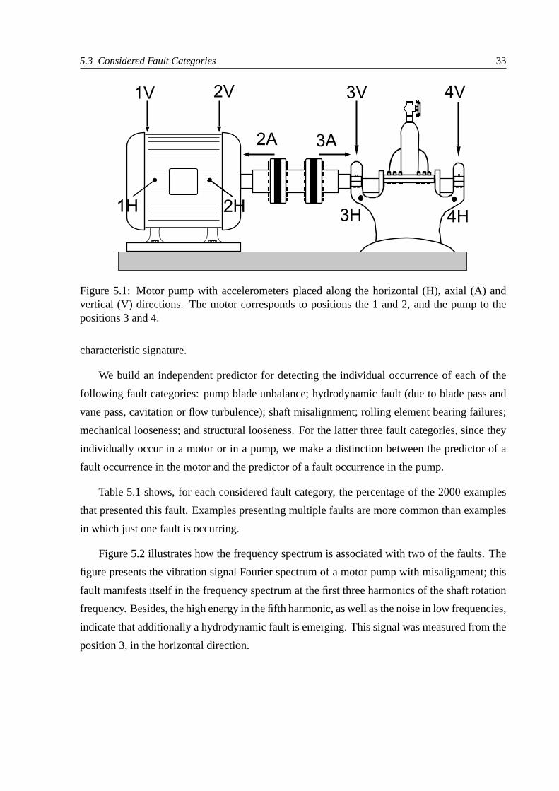
5.3 Considered Fault Categories 33

Figure 5.1: Motor pump with accelerometers placed along thehorizontal (H), axial (A) andvertical (V) directions. The motor corresponds to positions the 1 and 2, and the pump to thepositions 3 and 4.

characteristic signature.

We build an independent predictor for detecting the individual occurrence of each of the

following fault categories: pump blade unbalance; hydrodynamic fault (due to blade pass and

vane pass, cavitation or flow turbulence); shaft misalignment; rolling element bearing failures;

mechanical looseness; and structural looseness. For the latter three fault categories, since they

individually occur in a motor or in a pump, we make a distinction between the predictor of a

fault occurrence in the motor and the predictor of a fault occurrence in the pump.

Table 5.1 shows, for each considered fault category, the percentage of the 2000 examples

that presented this fault. Examples presenting multiple faults are more common than examples

in which just one fault is occurring.

Figure 5.2 illustrates how the frequency spectrum is associated with two of the faults. The

figure presents the vibration signal Fourier spectrum of a motor pump with misalignment; this

fault manifests itself in the frequency spectrum at the firstthree harmonics of the shaft rotation

frequency. Besides, the high energy in the fifth harmonic, as well as the noise in low frequencies,

indicate that additionally a hydrodynamic fault is emerging. This signal was measured from the

position 3, in the horizontal direction.

5.4 Extracted Features 34

0

0.5

1

1.5

2

2.5

0 200 400 600 800 1000

Velo

city

(mm

/s)

Frequency (Hz)

Figure 5.2: Vibration signal Fourier spectrum of a motor pump presenting misalignment andalso an emerging hydrodynamic fault.

Table 5.1: Fault occurrence.Fault class Percentage of faulty data

Misalignment 42.6%Hydrodynamic 42.4%Unbalance 24.9%Bearing - motor 24.9%Bearing - pump 16.6%Structural looseness - motor 26.6%Structural looseness - pump 13.9%Mechanical looseness - motor 12.1%Mechanical looseness - pump 8.6%

5.4 Extracted Features

Our general classification strategy is based on providing asmuch information as possible

in the initial feature extractionstage, and further using ensemble construction to automatically

prioritize more relevant features.

It would be desirable to extract features from distinct, complementary information sources,

for instance electrical current, chemical, thermal, and mechanical vibration sensors. Also, it

would be desirable to employ different signal preprocessing techniques, thus obtaining fea-

tures from different domains aiming to reflect complementary perspectives. For instance, for

mechanical vibration sensors, the features can include [Lei et al. 2010]: time domain statistical

features such as mean, root mean square (RMS), variance, skewness and kurtosis; frequency do-

main features such as the amplitude of the spectrum and the energy in specific frequency bands;


and time-frequency domain features obtained by using advanced time-frequency analysis tech-

niques, such as the empirical mode decomposition (EMD) and the wavelet packet transform

(WPT) [Lei et al. 2010].

But the information format of the acquired examples was previously fixed as the frequency

and the envelope spectrum of machine vibration signals. We work with well-established signal

processing techniques, namely the Fourier transform, envelope analysis based on the Hilbert

transform [Mendel, Rauber e Varejao 2008] and median filtering. Thus the extracted features

correspond to the vibrational energy of predetermined frequency bands of the spectrum.

In the initial feature extraction stage, we extract the samefeature categories for building the

predictor of every considered fault. The initially extracted feature set is composed of a total of

D = 81 features, with 68 of them from the Fourier spectrum and 13 of them from the Envelope

spectrum.

Before extracting theD = 81 features that globally describe the condition of a motor pump,

it is necessary to specify which one of the four machine positions will be employed as the source

of the vibration signal. This depends on which fault category is currently under consideration.

Specifically, the shaft misalignment predictor chooses

between position 2 or 3, actually selecting the one which presents the higher total RMS

vibration energy of the velocity signal, for the testing patternx under consideration. Similarly,

the predictor of unbalance or hydrodynamic fault chooses between positions 3 or 4. For me-

chanical looseness, structural looseness or a bearing defect, since they can independently occur

in a motor or in a pump, we build an independent predictor to detect a fault occurrence in the

motor (thus choosing between the position 1 or 2) and anotherindependent predictor to detect

a fault occurring in the pump (thus choosing between the position 3 or 4).

In summary, the complete diagnostic system is composed of nine independent SVM en-

sembles, each of which individually detects one consideredfault category.

5.4.1 Fourier Spectrum Features

We extract a total of 68 features from the Fourier spectrum. We use the RMS value of a

10% large narrow band around each of the following harmonicsof the shaft rotation frequency:

0.5x, 1x, 1.5x, 2x, 2.5x, 3x, 3.5x, 4x, 4.5x, 5x and 5.5x, obtained for each of the three directions

of measurement, namely horizontal, vertical and axial (this generates a total of 11× 3 = 33

features).


Besides, we use as features the sum of the RMS value of a 10% largenarrow band around

the harmonics 1x, 2x, ..., 5x, in each direction (3 features), and also similarly the sum of the

RMS value of bands around the inter-harmonics 0.5x, 1.5x, ..., 5.5x (3 features).

We also use the RMS value of the noise calculated with the median filtering, in the bands

0x-1x, 0x-2x, 0x-3x, 0x-4x and 0x-5x, in each direction (5×3= 15 features).

Additionally, we use the 10% large narrow band around harmonics of the pump blade pass

frequency (BPF), namely 0.5×BPF, 1.0×BPF and 2.0×BPF, in each direction (3× 3 = 9

features).

We also use the vibration signal total RMS value, in each direction for the velocity signal

(3 features) and in horizontal and vertical direction for the acceleration signal (2 features).

5.4.2 Envelope Spectrum Features

We extract a total of 13 features using the Envelope analysis[McInerny e Dai 2003]. Specif-

ically, these features correspond to the RMS of 10% large narrow bands around the first, the sec-

ond and the third harmonics of the bearing characteristic frequencies, namely BPFI, BPFO, FTF

and BSF [Mendel, Rauber e Varejao 2008], in the horizontal direction (this generates a total of

4×3= 12 features). The bearing characteristic frequencies depend of the bearing model of the

machine under consideration. We also use as a feature the total RMS value of the Envelope

spectrum (1 feature).

37

6 Experimental Results

“Computers are useless.

They can only give you answers.”

- Pablo Picasso.

This chapter shows the experimental results achieved by thestudied classification models,

using the acquired database of real-world industrial machine vibration signals.

Section 6.1 details the 5×2 cross-validation method, employed to estimate the quality of

the studied classification models which are presented in section 6.2. Section 6.3 provides the

classification accuracy estimated by 5× 2 cross-validation. Section 6.4 details experiments

performed to provide a better insight into important aspects of the proposed ensemble method.

6.1 Cross-validation 5×2 38

6.1 Cross-validation 5×2

To assess the effectiveness of the studied classification approaches we performed a strati-

fied 5×2 cross-validation [Kuncheva 2004]. This corresponds to five replications of a 2-fold

cross-validation. In each replication, the complete database of 2000 examples was randomly

partitioned, in a stratified manner, into two sets each one with approximately 1000 examples

(the stratification process preserves the distribution of the nine fault categories between both

sets). So in each replication each considered classification model for creating the predictor of a

fault was trained on a set and tested on the remaining one; after the five replications, the final

test data AUC achieved by this classification model in predicting this fault is then obtained as

the average of the ten estimated testing data AUC values.

6.2 Studied Classification Models

For each considered fault category, we studied four different classification models for build-

ing the predictor of this fault: a single SVM; a SVM ensemble built by the traditional GEFS

method, with every SVM using the same hyperparameter value;a SVM ensemble built by

a straightforward upgrade of GEFS, namely tuning the hyperparameters of every SVM ulti-

mately produced by GEFS; and a SVM ensemble built by the proposed multiple-GEFS method

described in chapter 4.

6.2.1 TheSVM Classification Model

This classification model is a single SVM classifier, using all theD = 81 available features.

We used the grid-search method to tune the hyperparameters as explained in section 4.3.

6.2.2 TheGEFS Classification Model

This classification model is a SVM ensemble built by the traditional GEFS method, de-

scribed in section 4.2.1. We employed the hyperparameter value (C = 8.0,γ = 0.5) to build

RBF-kernel C-SVMs to estimate fitness; this value was chosen since it was frequently selected

by grid-search in preliminary experiments, thus suggesting that this hyperparameter value tends

to produce more accurate SVMs.

We set the initial value of theλ regularization parameter used for fitness evaluation as

λ = 1.0. We useM = 20 classifiers (feature subsets) in the ensemble. In each generation,

6.2 Studied Classification Models 39

starting from theseM = 20 feature subsets, we producedmmut = 10 new feature subsets by

using mutation (randomly changing Percmut= 30% of features) and moremcro= 10 new feature

subsets by using cross-over; from theseM+mcro+mmut = 40 feature subsets, theM = 20 top

ones with higher fitness were selected to compose the ensemble at the end of this generation.

The population evolved for a total ofN = 100 generations.

A single run of the GEFS algorithm demanded a total of 20+N×20= 2020 feature subsets

to be evaluated. Since each feature subset evaluation corresponded to a 5-fold cross validation,

a run of the GEFS algorithm demanded a total of 2020×5= 10100 SVMs to be constructed.

In summary, thisGEFS classification model corresponds to an ensemble of 20 RBF-kernel

C-SVMs, each of which used the hyperparameter values(C= 8.0,γ = 0.5).

6.2.3 TheGEFS-Tuned Classification Model

This classification model corresponds to a straightforwardupgrade of GEFS, namely tuning

the hyperparameters of each SVM in an ensemble built by GEFS.First we used theGEFS

classification model (presented in section 6.2.2) to generate an ensemble ofM = 20 SVMs

which differ among themselves solely on their feature subset. Further, for each of these 20

produced SVMs we employed the grid-search method to tune itshyperparameters. Thus the

final ensemble was composed ofM = 20 SVMs which differ among themselves on their feature

subset and also on their employed hyperparameter value.

In summary, thisGEFS-Tuned classification model corresponds to an ensemble of 20

RBF-kernel C-SVMs, each of which used tuned hyperparameters.

6.2.4 TheMultiple-GEFS Classification Model

This classification model corresponds to a SVM ensemble based on feature and hyperpa-

rameter variation, built by the multiple-GEFS ensemble method proposed in this work (pre-

sented in section 4.1).

For creating the setF of feature subsets, we ranI = 5 independent GEFS searches, each of

which used a different, fixed hyperparameter value(C,γ)i to build SVMs to estimate the quality

of the feature subsets. After preliminary experiments to evaluate the hyperparameter values

investigated by the grid-search tuning method (which are presented in section 4.3), we defined

the following hyperparameter values to be used:{(C= 8.0,γ = 0.5), (C= 128.0,γ = 0.03125),

(C = 128.0,γ = 0.125), (C = 128.0,γ = 2.0), (C = 128.0,γ = 8.0)}. The former value was

6.3 Cross-validation 5×2 Estimated Results 40

chosen since it provided more accurate SVMs, while the latter values were chosen because they

correspond to a large range ofγ values besides using a relatively highC value. Every GEFS

search evolved for a total ofN = 100 generations.

To ultimately compose the setF of feature subsets we used the outputs of those five GEFS

searches, thus|F | = 5×20= 100. Further, for composing the SVM setH , for each feature

subset inF we used the grid-search method to build a SVM with tuned hyperparameters. Thus

|H |= |F |= 100. Finally, from all these|H |= 100 produced SVMs, we used the SFS search to

select a reduced SVM subsetE as explained in section 4.4. We set the ensemble size as|E |= 40,

so the ultimately produced ensembleE was composed of 40 SVMs. The other parameters of

the GEFS algorithm were set as for theGEFS classification model presented in section 6.2.2.

In summary, thisMultiple-GEFS classification model corresponds to an ensemble of 40

RBF-kernel C-SVMs, each of which used tuned hyperparameters.

6.3 Cross-validation 5×2 Estimated Results

Table 6.1 presents the testing data AUC values and the standard deviations estimated by

5×2 cross-validation. For each considered fault, the result of the classification model which

provided the most accurate predictor is showed in bold.

The consistently higher accuracy achieved by the proposedMultiple-GEFS classifica-

tion model, in comparison to the accuracy achieved by theGEFS or theGEFS-Tuned classi-

fication models, suggests the importance of employing a powerful search to deeply investigate

the space of feature subsets and the space of hyperparametervalues, aiming to produce an op-

timized SVM ensemble based on feature and hyperparameter variation. Results show that the

Multiple-GEFS classification model achieved the highest accuracy for every fault category,

and the lowest standard deviation for six of the nine considered faults.

To corroborate the superiority of the multiple-GEFS method, we used the statistical testing

procedure proposed by Dietterich (described in [Kuncheva 2004]) to be employed with the 5×2

cross-validation process, which determines whether the estimated difference of AUC values is

statistically significantly different.

The level of significance is the 0.05 percentile. For misalignment, hydrodynamic and

bearing-motor faults, the statistical test confirmed that the Multiple-GEFS classification

model performed significantly better than theGEFS or theGEFS-Tuned classification mod-

els. Also, comparing theMultiple-GEFS model to theSVM model (which corresponds to

6.4 Influence of the Number of Evolved Generations and the Number of Component SVMs 41

Table 6.1: Test data AUC estimated by 5×2 cross-validation

Fault category SVM GEFS GEFS-Tuned

Multiple-GEFS

Misalignment .834±.011 .862±.007 .865±.009 .882±.006

Unbalance .909±.014 .933±.008 .929±.006 .942±.005

Hydrodynamic .923±.010 .931±.012 .935±.010 .942±.008

Bearing - motor .935±.006 .955±.004 .957±.004 .969±.005

Bearing - pump .877±.020 .927±.014 .926±.019 .944±.010

Structural L. - motor .914±.009 .931±.006 .934±.007 .943±.008

Structural L. - pump .857±.028 .893±.011 .896±.012 .911±.013

Mechanical L. - motor .862±.013 .888±.012 .888±.012 .895±.012

Mechanical L. - pump .886±.022 .908±.016 .908±.018 .920±.014

a single SVM), the statistical test confirmed a significantlysuperior performance for all those

mentioned faults and additionally for the bearing-pump fault. On the other hand, for theGEFS

or theGEFS-Tuned classification models, the statistical test confirmed a superior performance

of the ensemble in comparison to a single SVM just for the bearing-motor fault.

6.4 Influence of the Number of Evolved Generations and theNumber of Component SVMs

In this section we show experimental results aiming to provide an insight into two important

aspects of the proposed ensemble method: the influence of thenumber of evolved generations

and the influence of the number of component SVMs in the ensembles.

6.4.1 Influence of the Number of Evolved Generations

An important parameter of the GEFS algorithm is the maximum number of evolved gen-

erations. Using a very high number of generations causes twomain problems, namely a high

computational cost and overfitting. In this work, to build the SVM ensembles, we evolved the

GEFS searches for a total ofN = 100 generations.


0 50 100 150 200 250 300 3500.83

0.84

0.85

0.86

0.87A

UC

onte

stda

ta

Number of evolved generations

Figure 6.1: AUC on test data achieved by each evolved generation of the GEFS method, for themisalignment predictor.

Figure 6.1 presents the behaviour of a GEFS search concerning the number of evolved

generations. The figure shows results obtained for the first pair of training and testing data

generated for the 5×2 cross-validation process, considering the misalignmentpredictor. One

can observe the AUC on test data achieved by the SVM ensemble produced by each generation

of theGEFS classification model, starting from the generation number 1and finishing in the

generation number 400; every SVM used the hyperparameter value (C = 8.0,γ = 0.5). It can

be seen that the generation number 100 corresponded to an ensemble with a relatively high

accuracy. The figure also shows that after the generation number 150 the test AUC presented

a tendency of decreasing, as a consequence of overfitting; surprisingly, the ensemble produced

by the generation number 400 presented a lower estimated test data AUC than the ensemble

defined by the first generation.

To present the behaviour found for some of the other faults, figures 6.2 and 6.3 present

results for the bearing - pump and the bearing - motor fault predictor, respectively; these experi-

ments also used the first pair of training and testing data generated by the 5×2 cross-validation.

6.4.2 Influence of the Number of Component SVMs

To provide an insight into the influence of the number of component SVMs in an en-

semble, we show the AUC on test data estimated during the classifier selection stage of the

Multiple-GEFS classification model, performed using the sequential forward selection (SFS)

search strategy.


0 50 100 150 200 250 300 3500.92

0.93

0.94

0.95

AU

Con

test

data


Figure 6.2: AUC on test data achieved by each evolved generation of the GEFS method, for thebearing - pump fault predictor.

0 50 100 150 200 250 300 3500.93

0.94

0.95

0.96

AU

Con

test

data


Figure 6.3: AUC on test data achieved by each evolved generation of the GEFS method, for thebearing - motor fault predictor.

6.5 Usefulness of Hyperparameter Tuning to Improve SVM Diversity 44

training data (selection criterion)

test data

0 10 20 30 40 50 60 70 80 90 1000.83

0.86

0.89

0.92

AU

C

Number of selected SVMs

Figure 6.4: AUC on training and testing data achieved by eachnumber of component SVMs,during the classifier selection stage of the multiple-GEFS method, for the misalignment predic-tor.

Figure 6.4 shows results for the first generated pair of train-test data of the 5× 2 cross-

validation, for the misalignment predictor. The figure presents the AUC of training data (which

is the selection criterion) and the AUC of testing data achieved by the SVM ensemble defined

by using each number of selected SVMs, from 1 SVM to 100 SVMs. The final ensemble was

composed of the|E | = 40 firstly selected SVMs, since we observed a general tendency of an

AUC decrease with the use of a larger set.

To present the behaviour found for some of the other faults, figures 6.5 and 6.6 present

results for the structural looseness - pump and the structural looseness - motor predictor, re-

spectively; these experiments also used the first pair of training and testing data generated by

the 5×2 cross-validation.

6.5 Usefulness of Hyperparameter Tuning to Improve SVMDiversity

This experiment provides an insight into the effectivenessof hyperparameter tuning aiming

to improve SVM diversity. First, we used feature selection to generate a set of different feature



test data

0 10 20 30 40 50 60 70 80 90 1000.79

0.82

0.85

0.88

0.91

0.94

AU

C


Figure 6.5: AUC on training and testing data achieved by eachnumber of component SVMs,during the classifier selection stage of the multiple-GEFS method, for the structural looseness -pump predictor.


test data

0 10 20 30 40 50 60 70 80 900.91

0.94

0.97

AU

C


Figure 6.6: AUC on training and testing data achieved by eachnumber of component SVMs,during the classifier selection stage of the multiple-GEFS method, for the structural looseness -motor predictor.


subsets. Further, for each produced feature subset, we estimated the classification accuracy

achieved by a SVM using this feature subset. We evaluated twoapproaches: building each

SVM with the hyperparameter value(C= 8.0,γ= 0.5) (which tends to provide accurate SVMs)

and building each SVM with a tuned hyperparameter.

To perform feature selection, we used the traditionally employed sequential forward selec-

tion (SFS) search strategy [Kudo e Sklansky 2000]. The SFS search was presented in section

4.4 in the context of selecting classifiers to compose an ensemble. But in the present section,

we use SFS to select features aiming to generate an accurate single SVM.

The SFS search starts with an empty set of selected features,and at each step one feature is

included in this set, namely the feature that provided the higher selection criterion with its indi-

vidual inclusion in the current set of selected features. The selection criterion of a feature was

estimated as the 5-fold cross-validation AUC achieved by a SVM using the currently selected

features and also this new feature under evaluation. The SVMs used the hyperparameter value

(C= 8.0,γ = 0.5).

From the total ofD = 81 available features, we required SFS to selectD−1= 80 features.

This produces 80 different feature subsets; for each one we evaluated two classifiers, namely a

SVM with fixed hyperparameters and a SVM with tuned hyperparameters.

Figure 6.7 presents the results obtained for the first pair oftraining and testing data defined

by 5×2 cross-validation, for the misalignment predictor. For each number of selected features,

from k = 1 to k = 80, the figure shows the AUC on the test data achieved by the SVMwith

hyperparameter fixed as(C = 8.0,γ = 0.5), and the AUC on test data achieved by the SVM

with tuned hyperparameters. Figure 6.7 also shows, as a horizontal line, the test data AUC

achieved by the SVM ensemble built by theMultiple-GEFS classification model.

By comparing the performance of the non-tuned SVMs versus thetuned SVMs, it is in-

teresting to see that tuning the hyperparameters of eachindividual SVM tends to increase the

collectivediversity of SVMs, since the figure shows that the AUC achieved by the tuned SVMs

can strongly vary even among SVMs that employ similar feature subsets (i.e. SVMs that use a

similar number of selected features). Such an improvement in SVM diversity is useful since it

corresponds to an increasing in the disagreement among the SVMs, which tends to improve the

ensemble accuracy. Indeed, the figure shows that the performance of the ensemble with tuned

SVMs (indicated as a dashed horizontal line) was significantly better than the performance of

any single SVM.

Figures 6.8 and 6.9 present results for the structural looseness - pump and the structural


non-tuned SVMs

tuned SVMs

multiple-GEFS

0 10 20 30 40 50 60 70 800.75

0.78

0.81

0.84

0.87

AU

Con

test

data

Number of selected features

Figure 6.7: AUC on test data achieved by the Multiple-GEFS method, and by individual SVMswhich use selected feature subsets with tuned or non-tuned hyperparamenters, for the misalign-ment predictor.


non-tuned SVMs

tuned SVMs

multiple-GEFS

0 10 20 30 40 50 60 70 800.77

0.80

0.83

0.86

0.89

AU

Con

test

data


Figure 6.8: AUC on test data achieved by the Multiple-GEFS method, and by individual SVMswhich use selected feature subsets with tuned or non-tuned hyperparamenters, for the structurallooseness - pump predictor.

looseness - motor predictor, respectively. Figures 6.10 and 6.11 present results for the me-

chanical looseness - pump and the mechanical looseness - motor predictor, respectively. These

experiments also used the first pair of training and testing data generated by the 5× 2 cross-

validation.


non-tuned SVMs

tuned SVMs

multiple-GEFS

0 10 20 30 40 50 60 70 800.85

0.88

0.91

0.94

AU

Con

test

data


Figure 6.9: AUC on test data achieved by the Multiple-GEFS method, and by individual SVMswhich use selected feature subsets with tuned or non-tuned hyperparamenters, for the structurallooseness - motor predictor.

non-tuned SVMs

tuned SVMs

multiple-GEFS

0 10 20 30 40 50 60 70 800.62

0.68

0.74

0.80

0.86

0.92

AU

Con

test

data


Figure 6.10: AUC on test data achieved by the Multiple-GEFS method, and by individual SVMswhich use selected feature subsets with tuned or non-tuned hyperparamenters, for the mechan-ical looseness - pump predictor.


non-tuned SVMs

tuned SVMs

multiple-GEFS

0 10 20 30 40 50 60 70 800.83

0.85

0.87

0.89

0.91

AU

Con

test

data


Figure 6.11: AUC on test data achieved by the Multiple-GEFS method, and by individual SVMswhich use selected feature subsets with tuned or non-tuned hyperparamenters, for the mechan-ical looseness - motor predictor.

51

7 Conclusions and Future Work

“Around computers it is difficult to find the

correct unit of time to measure progress.

Some cathedrals took a century to complete.

Can you imagine the grandeur and scope of a

program that would take as long?”

- ‘Epigrams in Programming’, SIGPLAN, Association for Computing Machinery, 1982.

This chapter summarizes the main results of this work, and offer concluding remarks.

Section 7.1 draws conclusions. Section 7.2 points out to future research.

7.1 Conclusions 52

7.1 Conclusions

In this work we presented a novel approach for creating a SVM ensemble with component

classifiers differing among themselves on the feature subset and the hyperparameter value they

use. The performed experiments show a consistent improvement in the prediction accuracy in

comparison to using a single accurate SVM or using the well-established GEFS method for

creating ensemble classifiers.

This work presented an optimization method to improve the prediction accuracy, which is

generally the main objective of classification. But it is important to note that this improvement

in accuracy demands an even higher growth of the computational cost, specially during training,

that demands building and evaluating several SVMs to investigate the space of feature subsets.

Fortunately, SVMs can naturally be employed using parallelcomputing in order to drastically

reduce the processing time.

7.2 Future Work

We plan to work on two main directions of future research. First, acquiring data from more

sources than just vibration signals. Second, improving theproposed SVM ensemble method,

specifically by increasing the accuracy gain provided by thehyperparameter variation stage.

7.2.1 Using Data from Different Sources

We plan to acquire more real-world data, from different machines and from more sources

than just vibration signals. Thus we plan to develop a multiparametric diagnostic system, which

uses vibration signals complemented with electrical signals such as current, power and torque;

besides, we plan to employ new features which carry specific information about the occurrence

of some faults, for instance structural resonance [Wandekokem et al. 2011].

The use of features from different sources might increase the prediction accuracy, since

more diversified information may become available, with each information source considering

a different perspective of the current motor pump condition. Classifier ensembles can naturally

take advantage of multiple information sources, since using features extracted from different

sources has a good potential for generating classifiers thatgive wrong predictions in different

regions of the global feature space.

As the SVM ensemble method proposed in this work relies on initially extracting as much

7.2 Future Work 53

features as possible and further using ensemble construction to automatically prioritize more

relevant features, we expect this method to be able to naturally deal with features from multiple

sources. For instance, considering that the available features comprise a total ofDvib vibra-

tional features andDelecelectrical features, than the GEFS searches can be employedto directly

investigate all theseDglobal= Dvib +Delec features. In this case, the generated feature subsets

would be composed of features from both electrical and vibrational sources, as a result of the

performed GEFS searches that automatically determine optimized feature subsets.

7.2.2 Using Particle Swarm Optimization to Tune Hyperparameters

The performed experiments showed the consistent improvement in SVM diversity and en-

semble accuracy that was provided by the hyperparameter tuning stage. Considering that in this

work we employed the simple, exhaustive grid-search methodto tune hyperparameters, there

is still much space for further improvement. Specifically, we plan to investigate more powerful

approaches to tune SVMs.

A straightforward improvement of the proposed SVM ensemblemethod may be employing

a more powerful method for tuning the hyperparameters of each produced SVM aiming to

directly increase its individual accuracy; this also implicitly increases the collective diversity of

SVMs.

A more complex improvement of the proposed SVM ensemble method may be using hy-

perparameter variation not only to increase the individualaccuracy of each SVM, but also to

directly improve the collective divergence of a set of SVMs. That is already done by the GEFS

method, but using feature variation instead of hyperparameter variation.

Particle Swarm Optimization (PSO) based techniques have been succesfuly employed for

SVM hyperparameter tuning [Li e Tan 2010]. By now, these approaches have showed promis-

ing results for building accurate single SVMs. Thus a straightforward improvement of the

proposed SVM ensemble method may be using a PSO search to tunehyperparameters, instead

of using the simple grid-search. Also, since PSO is a population-based search algorithm (like

GEFS), PSO seems approppriate to be used for the more complextask of tuning the hyperpa-

rameters of a set of SVMs aiming to directly increase their diversity and accuracy.

54

Bibliography

[Bellini, Filippetti e Capolino 2008]BELLINI, A.; FILIPPETTI, F.; CAPOLINO, G.-A. Ad-vances in diagnostic techniques for induction machines.IEEE Transactions on IndustrialElectronics, v. 55, 2008.

[Bertoni, Folgieri e Valentini 2005]BERTONI, A.; FOLGIERI, R.;VALENTINI, G. Bio-molecular cancer prediction with random subspace ensembles of support vector machines.Neurocomputing, v. 63, p. 535–539, 2005.

[Bishop 2007]BISHOP, C. M.Pattern Recognition and Machine Learning. Berlin: Springer,2007. ISBN 978-0387310732.

[Breiman 1996]BREIMAN, L. Bagging predictors.Machine Learning, v. 24(2), p. 123–140,1996.

[Brown et al. 2005]BROWN, G. et al. Diversity creation methods:a survey and categorization.Journal of Information Fusion, v. 6(1), 2005.

[Chen, Lin e Schölkopf 2005]CHEN, P. H.; LIN, C. J.; SCHöLKOPF, B. Atutorial onν-supportvector machines.Applied Stochastic Models in Business and Industry, v. 21, p. 111–136, 2005.

[Evgeniou, Pontil e Elisseeff 2002]EVGENIOU, T.; PONTIL, M.; ELISSEEFF, A. Leave-one-out error, stability, and generalization of voting combinations of classifiers.Machine Learning,2002.

[Fawcett 2006]FAWCETT, T. An introduction to ROC analysis.Pattern Recog. Letters, v. 27,2006.

[Freund e Schapire 1996]FREUND, Y.; SCHAPIRE, R. Experiments with a new boosting algo-rithm. In: Proc. 13th International Conference on Machine Learning (ICML’96). Bari, Italy:[s.n.], 1996.

[Ho 1998]HO, T. The random subspace method for constructingdecision forests.IEEE Trans-actions on Pattern Analysis and Machine Intelligence, v. 20(8), p. 832–844, 1998.

[Hu et al. 2007]HU, Q. et al. Fault diagnosis of rotating machinery based on improved waveletpackage transform and SVMs ensemble.Mechanical Systems and Signal Processing, v. 21, p.688–705, 2007.

[Islam, Yao e Murase 2003]ISLAM, M. M.; YAO, X.; MURASE, K. A constructive algorithmfor training cooperative neural network ensembles.IEEE Transactions on Neural Networks,v. 14(4), p. 820–834, 2003.

[Kim et al. 2003]KIM, H. C. et al. Constructing support vector machine ensemble.PatternRecognition, v. 36, p. 2757–2767, 2003.

Bibliography 55

[Kudo e Sklansky 2000]KUDO, M.; SKLANSKY, J. Comparison of algorithms that select fea-tures for pattern classifiers.Pattern Recognition, v. 33, p. 25–41, 2000.

[Kuncheva 2004]KUNCHEVA, L. I.Combining Pattern Classifiers. [S.l.]: Springer, 2004.

[Lei et al. 2010]LEI, Y. et al. A multidimensional hybrid intelligent method for gear fault diag-nosis.Expert Systems with Applications, v. 37, p. 1419–1430, 2010.

[Li e Tan 2010]LI, S.; TAN, M. Tuning SVM parameter by using a hybrid CLPSO-BFGF algo-rithm. Neurocomputing, v. 73, p. 2089–2096, 2010.

[Li, Wang e Sung 2008]LI, X.; WANG, L.; SUNG, E. Adaboost withSVM-based componentclassifiers.Engineering Applications of Artificial Intelligence, v. 21, 2008.

[McInerny e Dai 2003]MCINERNY, S. A.; DAI, Y. Basic vibration signal processing for bear-ing fault detection.IEEE Transactions on Education, v. 46, n. 1, p. 149–156, 2003.

[Mendel, Rauber e Varejao 2008]MENDEL, E.; RAUBER, T. W.; VAREJAO, F. M. Automaticbearing fault pattern recognition using vibration signal analysis. In: Proc. of the IEEE Int.Symp. on Ind. Electronics ISIE 2008.[S.l.: s.n.], 2008.

[Miller et al. 2001]MILLER, K. R. et al. An introduction to kernel-based learning algorithms.IEEE Transactions on Neural Networks, v. 12, p. 181–201, 2001.

[Opitz e Maclin 1999]OPITZ, D.; MACLIN, R. Popular ensemble methods: An empiricalstudy.Journal of Artificial Intelligence Research, v. 11, p. 169–198, 1999.

[Opitz 1999]OPITZ, D. W. Feature selection for ensembles. In: Proc. of the Sixteenth NationalConf. on Artificial Intelligence AAAI’99. [S.l.: s.n.], 1999.

[Sun, Zhang e Wang 2007]SUN, B.-Y.; ZHANG, X.-M.; WANG, R.-J. On constructing andpruning SVM ensembles. In:Proc. of the 2007 IEEE Conf. on Signal-Image Technologies.[S.l.: s.n.], 2007.

[Theodoridis e Koutroumbas 2006]THEODORIDIS, S.; KOUTROUMBAS, K. Pattern Recog-nition, Third Edition. Orlando, FL, USA: Academic Press, Inc., 2006. ISBN 0123695317.

[Tsymbal, Pechenizkiy e Cunningham 2005]TSYMBAL, A.; PECHENIZKIY, M.; CUN-NINGHAM, P. Diversity in search strategies for ensemble feature selection.Information Fu-sion, v. 6, p. 83–98, 2005.

[Tu et al. 2007]TU, C.-J. et al. Selection using PSO-SVM.IAENG International Journal ofComputer Science, v. 33, p. 111–116, 2007.

[Valentini e Dietterich 2000]VALENTINI, G.; DIETTERICH, T. G. Bias-variance analysis ofsupport vector machines for the development of SVM-based ensemble methods.The Journalof Machine Learning Research, 2000.

[Vapnik 1998]VAPNIK, V.The Nature of Statistical Learning Theory. New York: Wiley, 1998.

[Verikas et al. 2010]VERIKAS, A. et al. Selecting features from multiple feature sets for SVMcommittee-based screening of human larynx.Expert Systems with Applications, v. 37, p.6957–6962, 2010.

Bibliography 56

[Wandekokem et al. 2011]WANDEKOKEM, E. D. et al. Diagnosingmultiple faults in oil rigmotor pumps using support vector machine classifier ensembles.Integrated Computer-aidedEngineering, v. 18, 2011.

[Widodo e Yang 2007]WIDODO, A.; YANG, B. S. Support vector machine in machine condi-tion monitoring and fault diagnosis.Mechanical Systems and Signal Processing, v. 21, 2007.

[Zio, Baraldi e Gola 2008]ZIO, E.; BARALDI, P.; GOLA, G. Feature-based classifier ensem-bles for diagnosing multiple faults in rotating machinery.Applied Soft Computing, v. 8, p.1365–1380, 2008.

57

APPENDIX A -- Attached reference

Attached is the paper "Diagnosing multiple fault in oil rig motor pumps using support vector

machine classifier ensembles", Integrated Computer-Aided Engineering, vol. 18, 2011.

Diagnosing multiple faults in oil rig motorpumps using support vector machine classifierensemblesEstefhan Dazzi Wandekokem1∗, Eduardo Mendel1, Fabio Fabris1,Marcelo Valentim1, Rodrigo J. Batista2, Flavio M. Varejao1, and Thomas W. Rauber1.

1Department of Computer Science, Federal University of Espırito SantoAv. Fernando Ferrari s/n, 29075-910 Vitoria, ES, Brazilphone: + (55) 27 3335-2654; fax: + (55) 27 3335-2850;email:{estefhan, emendel, ffabris, marcelo, fvarejao, thomas}@inf.ufes.br2Espırito Santo Exploration and Production Business UnitPetroleo Brasileiro S.A. PETROBRAS, Av. Fernando Ferrari 1000,29075-973 Vitoria, ES, Brazil,email: [email protected]

Abstract.We present a generic procedure for diagnosing faults using featuresextracted from noninvasive machine signals, based onsupervised learning techniques to build the fault classifiers. An importantnovelty of our research is the use of 2000 examples ofvibration signals obtained from operating faulty motor pumps, acquired from 25 oil platforms off the Brazilian coast during fiveyears. Several faults can simultaneously occur in a motor pump. Each fault is individually detected in an input pattern by using adistinct ensemble of support vector machine (SVM) classifiers. We propose a novel method for building a SVM ensemble, basedon using hill-climbing feature selection to create a set of accurate, diverse feature subsets, and further using a grid-search parametertuning technique to vary the parameters of SVMs aiming to increase their individual accuracy. Thus our ensemble composingmethod is based on the hybridization of two distinct, simple techniques originallydesigned for producing accurate single SVMs.The experiments show that this proposed method achieved a higher estimated prediction accuracy in comparison to using a singleSVM classifier or using the well-established genetic ensemble feature selection (GEFS) method for building SVM ensembles.

1 Introduction

The detection and diagnosis of faults in complexindustrial machines is advantageous for economicaland security reasons [7]. The early detection of afault allows damaged components to be repaired dur-ing planned maintenance, which minimizes machinerydowntime besides providing more secure operations.Recent progress in sensor technology and computa-tional intelligence permit the construction of powerfuldiagnostic systems, which can aid relatively unskilled

operators in making reliable decisions about the ma-chine condition as well as providing valuable informa-tion to experts in making decisions about intricate faultoccurrences.

A single reliable diagnosis procedure for any type offault based on noninvasive signals is still not established[1]. Noninvasive monitoring relies on easily measuredsignals, for instance electrical and mechanical quanti-ties like current, voltage, flux, torque and speed. Inthis work we present a generic procedure for diagnos-ing faults using features extracted from machine sig-

58

nals. Our approach is based on thesupervised learning[2] classification paradigm as the primal mechanism toautomatically generate fault classifiers in a model-freecontext. This has as an advantage the requirement ofa minimum of a priori knowledge about the plant, asthe fault predictor is automatically defined based on thetraining data, which allows the diagnosis procedure tobe easily extended to many types of equipments, faultsand sensors.

Supervised learning based diagnosis requires the useof a large number of labeled examples of each fault cat-egory in order to build a classifier with a good gen-eralization capacity. An important novelty of our re-search is the use of data from real-world operating in-dustrial machines instead of using data from a con-trolled laboratory environment which is almost alwaysfound in the literature (see for instance [34]). This ishighly desirable, as laboratory hardware cannot realis-tically represent intricate real-world fault occurrences.We work with 2000 examples of vibration signals ob-tained from operating partially faulty motor pumps, ac-quired from 25 oil platforms off the Brazilian coast dur-ing five years. After extensive analysis, human expertsprovided a label for every fault present in each acquiredexample, relying on their practical experience in main-tenance engineering.

Several faults can simultaneously occur in a motorpump. We formulate the fault diagnosis problem as amulti-label [26] classification task in which several la-bels (fault categories) may be simultaneously assignedto a pattern; in this context, a pattern represents the sig-nals of a motor pump and a label represents a specificfault category. Each fault is individually detected in aninput pattern by a distinct binary predictor. Specifically,each fault category is detected by a distinctensemble[14] of support vector machine(SVM) [4] classifiers.The SVM classifier is currently considered one of themost powerful binary classification techniques; to fur-ther increase the accuracy of a single SVM we use anensemble of SVMs, composed of accurate SVMs thatdisagree on their predictions as much as possible. AnSVM ensemble assigns a patternx to the positive classωposor to the negative classωneg, with the positive classmeaning that the fault considered by the ensemble ispresent in the patternx and the negative class meaningthat this considered fault is not present inx (but other

faults may be present). We build a fault predictor ableto diagnose six fault categories, so it is composed ofsix independent ensembles of SVM classifiers, each en-semble considering the occurrence of a different fault.

We propose a novel method for building an accurateSVM ensemble. By now very few papers have inves-tigated SVM ensembles based on varying the featureset of the classifiers besides also varying their SVM pa-rameter value. It can be expected that using differentfeature subsets and SVM parameter values might in-crease the divergence among the SVMs in an ensem-ble, therefore increasing the ensemble accuracy. Wepropose a novel method for constructing an SVM en-semble, based on using hill-climbingfeature selection[11] to create a set of accurate, diverse feature sub-sets, and further using a grid-searchparameter tuningtechnique to vary the parameters of SVMs aiming toincrease their individual accuracy. Thus our ensem-ble composing method is based on the hybridizationof two distinct, simple techniques originally designedfor producing accurate single SVMs. The experimentsshow that this proposed method achieved a higher esti-mated prediction accuracy in comparison to other well-established approaches for building ensembles.

The remainder of this paper is organized as follows.Section 2 is concerned with the motor pump equipment,the considered fault categories and the extracted fea-tures. Section 3 details feature selection. Section 4describes the SVM classifier. Section 5 presents the en-semble approach for classification. Section 6 details theproposed method for building SVM ensembles basedon varying both the features and the parameters of theclassifiers. In section 7 we show the experimental re-sults achieved by the studied classification models. Fi-nally, section 8 draws conclusions and points out futureresearch.

2 Model-free approach to motor pump fault diag-nosis

There are two main approaches to the machinefault diagnosis problem: model-based techniques andmodel-free techniques. The model-based approach re-lies on an analytical model of the studied process, in-volving time dependent differential equations. In this

59

Figure 1: Horizontal motor pump with extended cou-pling between the motor and the pump. Accelerometersare placed along the main directions to capture specificvibrations of the main axes (H=horizontal, A=axial,V=vertical.)

case, usually the experimental process setup is installedon a controlled laboratory environment and is embed-ded in a control loop in which inputs, controlled vari-ables and sensor outputs are modeled. However in real-world processes the availability of an analytical modelis often unrealistic or inaccurate due to the complexityof the process. In this case model-free techniques are analternative approach [6]. This paper is concerned withmodel-free diagnosis of multiple faults in motor pumps,relying on supervised learning based techniques.

2.1 Motor pump equipment

Rotating machinery covers a wide range of mechan-ical equipment and plays an important role in industrialapplications. In this work we focus on a specific rotat-ing machine model, namely the horizontal motor pumpwith extended coupling between the electric motor andthe pump. Accelerometers are placed at strategic posi-tions along the main directions to capture specific vi-brations of the main shaft which provides a multichan-nel time domain raw signal. Figure 1 shows a typicalpositioning configuration of the accelerometers on theequipment.

2.2 Considered fault categories

Several faults can simultaneously occur in a motorpump. Such a high diversity of defects has a direct im-

0

0.5

1

1.5

2

2.5

0 200 400 600 800 1000

Vel

ocity

(m

m/s

)

Frequency (Hz)

Figure 2: Misalignment fault and its manifestation inthe frequency spectrum at the first three harmonics ofthe shaft rotation frequency. The high energy in the fifthharmonic, as well as the noise in low frequencies indi-cate that additionally a hydrodynamic fault is emerging.

pact on the subsequent classifier. For instance, manyfaults cause vibrations in similar frequency bands, likethe first, the second, and the third harmonics of the shaftrotation frequency, in such a way that the faults cannotbe detected by just searching for their well-known char-acteristic signature.

We build a predictor for individually detecting eachof the following six fault categories in an input pattern:rolling element bearing failures (problems on ball passinner raceway, ball pass outer raceway, or on bearingcage); pump blade unbalance; hydrodynamic fault (dueto blade pass and vane pass, cavitation or flow turbu-lence); shaft misalignment; mechanical looseness; andstructural looseness.

Figure 2 illustrates how the frequency spectrum is as-sociated with two of the faults, presenting the Fourierspectrum of the vibration signal (measured from theposition three, horizontal direction) of a faulty motorpump with a misalignment fault and also an emerginghydrodynamic fault.

Every example in the database of 2000 machine sig-nal acquisitions presented the occurrence of at least onefault. Examples presenting the occurrence of multiplefaults are more common than examples in which justone fault is occurring. Table 1 shows, for each of thesix considered fault categories, the percentage of the2000 examples that presented this fault.

60

Table 1: Fault occurrence.

Fault classA priori classdistribution

Misalignment 42.6%Hydrodynamic 42.4%Bearing 35.7%Unbalance 24.9%Structural looseness 21.2%Mechanical looseness 12.0%

2.3 Extracted features

The first step to diagnose the faults in a motor pumpis to extracta global feature vectorG to describe manyrelevant aspects of the current motor pump condition.The general strategy is to provide as much informa-tion as possible in the feature extraction stage and fur-ther use feature selection and ensemble construction toprioritize more relevant features. So the feature vec-tor G should be composed of features extracted fromdistinct, complementary information sources, for in-stance electrical current, chemical, thermal, and me-chanical vibration sensors. Also, for each informa-tion source, different signal preprocessing techniquesshould be used, thus producing features extracted fromdifferent domains that can reflect complementary per-spectives. For instance, for mechanical vibration sen-sors, the extracted features can include [16]: time do-main statistical features such as mean, root mean square(RMS), variance, skewness and kurtosis; frequency do-main features such as the amplitude of the spectrumand the energy in the frequency band considered by afeature; and time-frequency domain features obtainedby using advanced time-frequency analysis techniques,such as the empirical mode decomposition (EMD) [16]and the wavelet [22] packet transform (WPT) [16].

In this work we build a diagnostic system that usesvibration signals. We work with well-established signalprocessing techniques, namely the Fourier transform,envelope analysis based on the Hilbert transform [21]and median filtering. The reason that we use solely vi-bration signals besides not using other signal sourcesas for instance electrical current is that the information

format of the acquired examples was previously definedonly as the frequency and the envelope spectrum of themachine vibration signals. In this context, features cor-respond to the vibrational energy in a predeterminedfrequency band of the spectrum.

To build the predictor of a specific fault, an importantaspect to analyze is the occurrence of the fault in eachof the four machine positions of signal acquisition. Forinstance, the hydrodynamic fault only occurs in a pump(positions 3 and 4), the occurrence of a misalignmentfault is better detected by measuring vibrations close tothe shaft (positions 2 and 3), and the mechanical loose-ness fault usually occurs independently in a motor (po-sitions 1 and 2) or in a pump (positions 3 and 4).

We performed preliminary experiments aiming to de-fine a set of relevant features to be extracted. The cardi-nality of a feature vectorG is 95 regardless of the faultunder consideration, with 69 of them from the Fourierspectrum and 26 of them from the envelope spectrum.

2.3.1 Fourier spectrum features

For extracting features from the Fourier spectrum,for the hydrodynamical fault predictor, one feature vec-tor is extracted from the machine position which has thehighest total root mean square (RMS) value of the ve-locity signal selected from position 3 or 4 (the pump);for misalignment, one feature vector is similarly ex-tracted from position 2 or 3 (which are close to theshaft); for unbalance, 3 or 4; and for the bearing faultpredictor, from position 1, 2, 3 or 4. On the other hand,for structural looseness and mechanical looseness, onepattern is extracted from position 1 or 2 (motor) andanother distinct pattern is extracted from position 3 or4 (pump). A motor pump is diagnosed as faulty if anyof the extracted feature vectors is diagnosed as faulty,so the SVM classifiers of the first group of faults aretrained with one pattern per machine signal acquisition,while for the second group of faults a SVM is trainedwith two patterns per acquisition (each of which inde-pendently labeled as belonging to the positiveωpos orto the negativeωneg class).

Most of the Fourier features correspond to the RMSvalue of frequency bands defined as harmonics of theshaft rotation frequency, which is 60Hz for most of thestudied motor pumps (thus in this example 1x means 60

61

Hz and 1.5x means 90 Hz). We use the RMS value ofa 10% large narrow band around each of the followingfrequencies: 0.5x, 1.0x, 1.5x, ..., 5.5x, obtained for eachof the three directions of measurement (horizontal, ver-tical and axial) (which generates 3×11= 33 features,for instance the featurerms V 2.0x corresponds to thevertical direction and to the second harmonic). Besides,we take as features the sum of the RMS value of a 10%large narrow band around the harmonics 1x, 2x, ..., 5x,in each direction (3 features, for instancesum harm Xwhich corresponds to the axial direction), and also sim-ilarly the sum of the RMS value of bands around theinter-harmonics 0.5x, 1.5x, ..., 5.5x (3 features, for in-stancesum interharm H which corresponds to the hor-izontal direction). We also use the RMS value of thenoise calculated with the median filtering, in the bands0x-1x, 0x-2x, 0x-3x, 0x-4x and 0x-5x, in each direc-tion (3× 5 = 15 features, for instancenoise 0-4x Hwhich corresponds to the band 0x-4x and to the hori-zontal direction). Additionally, we use the 10% largenarrow band around harmonics of the pump blade passfrequency (BPF), namely 0.5×BPF, 1.0×BPF and2.0×BPF, in each direction (3×3= 9 features, for in-stancebpf 1x X which corresponds to BPF frequencyand to the axial direction). We also use the vibrationsignal total RMS value, in each direction for the veloc-ity signal (3 features, for instancetotal rms HV whichcorresponds to the horizontal direction) and in hori-zontal direction for the acceleration signal (1 feature,total rms HA). Finally we take the total RMS valueof the acceleration signal in the horizontal direction,specifically for position 1 or 2 (1 feature,rms motor A)and also 3 or 4 (1 feature,rms pump A).

2.3.2 Envelope spectrum features

For extracting features from the Envelope spectrumto compose a pattern, regardless of the fault under con-sideration, a group of features is taken from position1 or 2 (selecting the one with the highest total RMSvalue) and another group of features is similarly takenfrom position 3 or 4. Each group is composed of fea-tures defined as the RMS of 10% large narrow bandsaround the first, the second and the third harmonicsof the bearing characteristic frequencies [21] (BPFI,BPFO, FTF and BSF, each one being a constant value

determined by the machine bearing model), in the hor-izontal direction (the only one available for the Enve-lope signals), for instance the featurebpfo pump 2xcorresponds to the second harmonic of the BPFO fre-quency and is extracted from the pump (position 3 or4), and the featurebsf motor 1x corresponds to theBSF frequency and is extracted from the motor (posi-tion 1 or 2). We also use as a feature the total RMSvalue of the vibration signal Envelope spectrum, for in-stance the featurerms pump E which is extracted fromthe pump. Once a group of Envelope spectrum featuresis extracted from position 1 or 2 and another from posi-tion 3 or 4, they result in a total of 2×13= 26 features.

3 Feature selection

A central issue in fault diagnosis is the definition ofwhich aspects of the input signals, i. e. features, afault predictor should analyze. The traditional approachis the manual definition of the used features (see forinstance [17]). But the handpicking of the fault de-scriptive features demands specialized knowledge andcan result in predictors with low accuracy, for instancedue to multiple coexistent faults [30]. An approach foravoiding the manual definition of the important featuresrelies on the initial extraction of a large, comprehensivefeature set, and on the further use offeature selectiontechniques [11] to retain a reduced set of relevant fea-tures that are used to form the feature space of a classi-fier (see for instance [32]). An alternative approach isassigning a different weight to each of the extracted fea-tures [15]. In this work we use feature selection tech-niques to create a SVM classifier ensemble instead ofsearching for a single accurate SVM.

Feature selection is the process of choosing an opti-mized subset of features for classification from a largerset that may contain irrelevant and redundant informa-tion. The two common approaches to feature selectionare the filter and the wrapper methods. The former as-sess the saliency of feature subsets from data properties,without training a classifier. The latter uses the learn-ing algorithm itself to estimate the usefulness of fea-tures by evaluating classifiers which use the candidatefeature subsets. Wrappers methods are computationallymore expensive but usually allow more accurate feature

62

subsets to be found [24] and thus are used in this work.Feature selection is composed of two ingredients: the

selection criterion and the search strategy. The selec-tion criterion is used to estimate the performance of afeature subset. A suboptimal search strategy is neededsince an exhaustive search is not feasible to investigatethe space of feature sets.

3.1 Selection criterion

We estimate the criterionJ(Xk) of a candidate featuresetXk as the Area Under the ROC Curve (AUC) [10]achieved by a SVM classifier which usesXk, estimatedby cross-validation on the training data.

The Receiving Operating Characteristics (ROC)analysis is very useful for comparing classifiers in prob-lems with unbalanced classes in which negative classexamples are usually much more common than posi-tive ones. Table 1 shows that the predictor of someconsidered fault categories (for instance mechanicallooseness) must deal with the unbalance problem. AROC graph represents a classifier as a point in a two-dimensional space where the true positive rate is plot-ted on the Y axis and the false positive rate is plotted onthe X axis. The threshold of the estimated a posterioriprobability of belonging to the positive classωpos is setto 0.5 by default, producing the X-Y point. By vary-ing the threshold between zero and one, the X-Y pointtraces the ROC curve and a high area under it indicatesan accurate classifier; an AUC value of 0.5 correspondsto a random classifier. So the AUC value can be seenas the probability that, given a positive class examplep and a negative class examplen, both randomly sam-pled, the classifier outputsPpos(p)> Ppos(n).

3.2 Search strategy

An exhaustive search takes(|G|

d

)

attempts to selectdfeatures from an available global poolG of |G| features,which is computationally unfeasible in general. Thuswe must rely on a suboptimal search strategy.

We use theSequential Backward Selection(SBS)[13] search strategy, which operates based on a hill-climbing greedy search. The SBS strategy allows themore important features to be prioritized, which is use-ful for building accurate SVMs and thus accurate en-

sembles. The SBS method starts with every feature(from the global poolG) included in the set of selectedfeatures, and at each step one feature is removed fromthis set. Consider thatk features are included in theset of selected featuresXk. To remove the worst fea-ture fromXk, each currently selected featureξ j must beevaluated by being individually removed fromXk andranked following the criterionJ, so that

J(Xk \{ξ1})≥ J(Xk \{ξ2})≥ . . .≥ J(Xk \{ξk}). (1)

As a result of the current exclusion step, the updatedselected feature set is given asXk−1 = Xk\{ξ1}, having|Xk−1| = (k− 1) features in it. The exclusion processstops when the desired number of features is selected.

4 The support vector machine classifier

The support vector machine (SVM) [4] classificationarchitecture has been extensively used during the lastdecade in many distinct domains, for instance bioin-formatics [33] and machine fault diagnosis [31], andis currently considered one of the most powerful meth-ods in machine learning for solving binary classifica-tion problems; SVMs also have been successfully usedfor regression tasks [20]. We experimentally comparedSVM classifiers with Multi-layer Perceptron (MLP)[2] artificial neural network classifiers and found thatSVMs achieved a consistent higher accuracy, besidesthe MLP being computationally much more expensiveduring training and thus less appropriate to be used forfeature selection.

The objective of the SVM training is to create amaximum-margin separating hyperplane that lies in atransformed feature space defined implicitly by a ker-nel mapping. The hyperplane splits the mapped spaceinto two regions, one associated to the positive classωpos and the other to the negative classωneg; a SVMconsiders a patternx as belonging to the positive classωpos if x presents the fault category considered by theSVM or as belonging to the negative classωneg if x doesnot present this fault. The distance of a patternx to theseparating hyperplane, followed by a logistic discrim-ination, is used to estimate the a posteriori probabilityPpos(x) thatx belongs to the positive classωpos.

63

We use a widely adopted SVM model, namely a Ra-dial Basis Function (RBF) kernel and the C-SVM ar-chitecture [2]. So we work with two SVM parameters,namely the regularization parameterC which controlsthe model complexity and the kernel parameterγ whichcontrols the nonlinear mapping of the features.

The performance of a SVM classifier strictly dependson its parameters. We use an effective, simple methodto tune the SVM parameters, namely thegrid-searchon the log-scale of the parameters in combination withcross-validation on each candidate parameter vector.Basically, pairs(C,γ) from a set of predefined valuesare tried by evaluating SVMs which use them, and thepair that provided the highest cross-validation accuracydefines the best parameters.

We use thelibsvm library [3] to implement the SVMclassification.

5 Classifier ensembles

Combining decisions of multiple accurate, divergentpredictors into an ensemble decision is becoming oneof the most important techniques to improve classifica-tion accuracy [34]. In this context divergence meansthat each classifier gives erroneous answers in a dif-ferent region of the global feature space. Creating aso-calledclassifier ensembleentails addressing two is-sues: the construction of the base classifiers which con-stitute the ensemble and the combination of their in-dividual predictions. To combine classifier predictionswe use an effective, simple method, namely averagingthe scores assigned to an input pattern by the classifiersbeing combined.

The focus of this work is on methods for buildinga set of classifiers to compose an ensemble. By now,three approaches have become popular for achieving di-versity in an ensemble: using a different set of trainingdata for each classifier; using a distinct feature set foreach classifier; and setting different values of the clas-sifier intrinsic parameters.

5.1 Data-based ensembles

The classical approach to create a set of classifiers tocompose an ensemble relies on using a different train-ing data set for each classifier. For instance, in bagging

[2], each classifier in the ensemble samplesN trainingpatterns (with equal probability and with replacement)from an available set ofN different examples; so thetraining set of a classifier might not contain some of theavailable patterns besides containing some patterns thatare repeated.

Bagging works well with unstable classifiers, for in-stance MLP neural networks, in which a small variationof the training data set may cause a large variation ofthe classifier decision function. But the SVM is a stableclassifier, in the sense that a small variation of the train-ing data set tends to cause a small variation of the SVMdecision function, as just a reduced subset of the train-ing patterns are retained as support vectors (namely theones close to the decision boundary). Although someworks have reported that SVM ensembles built by us-ing bagging achieved a high prediction accuracy [12],other works have reported negative experiments aboutbagging based SVM ensembles [8]; see for instance [9]which stated that single SVMs with tuned parametersperformed as well as SVM ensembles built by usingthe bagging method. For the fault diagnosis problemstudied in this work we found that the traditional bag-ging method was not effective to increase the accuracyachieved by a single SVM.

5.2 Feature-based ensembles

A useful approach for building an ensemble is to em-ploy a different feature set for each classifier; see [34]for a reference on fault diagnosis.

Opitz [23] proposed the genetic ensemble feature se-lection (GEFS) method which relies on a Genetic Al-gorithm (GA) based search to investigate the space offeature sets. In GEFS, a member of the population (achromosome) represents the feature set of a single clas-sifier. Starting with randomly defined feature sets, thegenetic operators (selection, cross-over and mutation)are used to evolve the population aiming to increase theclassifiers fitness. The fitness of a classifier is estimatedas a linear combination of its accuracy and its diversity,the latter being defined as the average difference be-tween the prediction of this classifier and the predictionof the current ensemble. At the end of every generationthe algorithm outputs the feature subsets of the classi-fiers in the current ensemble, thus the last generation

64

defines the final produced feature subsets.Previous work shows that the GEFS method usually

achieves a higher prediction accuracy in comparison toother approaches for building ensembles [28]. Inspiredby GEFS, other GA based methods for building feature-based ensembles have been investigated; see [25] for areference on SVM ensembles.

5.3 Parameter-based ensembles

A natural approach for generating divergence amongthe decisions of a set of classifiers is the use of differentclassifier intrinsic parameter values. For instance, oneof the first studied ensemble models was an ensemble ofMLP neural network classifiers with each MLP havinga different number of neurons in its hidden layer. Con-sidering SVM classifier ensembles, varying the kernelparameter (in our case the RBFγ) of a SVM classifierdecisively changes its decision function [29], so usingdifferent kernel parameter values might allow the con-struction of divergent SVMs which is useful for build-ing ensembles [19]. For instance, in [27] an SVM en-semble was built with each SVM using a different pre-defined value forγ (every SVM used the same value forthe parameterC).

In this work, we use the grid-search parameter tun-ing technique to vary the parameters of SVMs aim-ing to increase their individual accuracy. Although thegrid-search method does not directly work aiming toincrease a metric of the diversity among the classifiers,we observed that the tuned SVM parameter value as-signed to each SVM was likely to be distinct amongmany of the produced SVMs, as each SVM used a dis-tinct feature subset. Thus this parameter tuning processis useful for building accurate SVMs which are also di-vergent among themselves.

6 The Best Selected Feature Subsets method

We propose a novel method for building an SVM en-semble, based on varying the features and also the valueof the parameters of the classifiers. We call it Best Se-lected Feature Subsets (BSFS). By now very few pa-pers have investigated SVM ensembles based on vary-ing both features and parameters. It can be expectedthat using different feature subsets and also parameter

values might increase the collective divergence amongthe SVM classifiers in an ensemble, therefore increas-ing the ensemble accuracy.

The BSFS method operates as follows. We use com-plementary SBS feature selection searches combinedwith the grid-search parameter optimization techniqueto build a large setL of classifiers that are candidatesto constitute the ensemble. Further we use a sequen-tial forward search to select just a reduced, optimizedsubsetE of them to compose the final ensemble. Thisapproach of building a large classifier setL and furthersearching for a subsetE is known asoverproduce-and-choose[14].

As we combine the decisions of the classifiers by av-eraging the assigned scores, an ensembleE estimatesthe probabilityPpos(x) that an input patternx belongsto the positive classωposas the average of thePpos(x)ch

classification score values that the classifierch in E out-puts forx (considering every classifier in the ensembleE i. e. for h= 1 to h= |E |). Thusx is predicted as be-longing toωpos if Ppos(x)> 0.5 or as belonging toωneg

otherwise.

6.1 The classifier overproduction stage

To create the setL of candidate classifiers to com-pose the ensemble, we first build a setΞ of feature setscomposed of several promising feature sets. The fea-ture sets use features from the global poolG and differon their cardinality. To defineΞ we performm distinctSBS feature selection searches,{S1, . . . ,Si , . . . ,Sm},which differ among themselves on the SVM parametervalue they use to create SVMs to estimate the selectioncriterion; this allows feature subsets to be found usingcomplementary kernel mapped feature spaces. We re-quire each searchSi to select a total of 1 feature (whichis equivalent to requireSi to exclude|G|−1 features);the exclusion of each feature defines a new feature sub-set and hence a new candidate classifier to composethe ensemble. So the feature sets inΞ are determinedby taking each produced feature setXSi

k which useskfeatures selected by the searchSi , considering everykandi, that isk= 1,2,3, . . . , |G| andi = 1,2, . . . ,m (thus|Ξ|= m×|G|).

Then the classifier setL is defined by building, foreach feature setXSi

k in the setΞ, a classifiercSik that uses

65

ECSG

k=|G|

Sm

k=1

Sm

k=|G|

S1

k=1

S1

Xk=1

S1

Xk=|G|

S1

Sm

Xk=1

Xk=|G|

Sm

E

Ensemble

Classifier

selection

method

Set of candidate

classifiers

k

SiInduced

classifiersXk

SiSelected feature

sets (with size k)

i

Feature

selection

methods S

Global pool

of feature G

S1

Sm

Figure 3: A diagram of the training process of an ensemble built by the BSFS method (used as the predictor ofa fault). After the initial overproduction stage every candidate SVM classifier in the setL uses a distinct featuresubset (defined by feature selection) and also tuned parameters. In the Ensemble Classifier Selection (ECS) stage theensemble is finally built by selecting an optimized subset ofclassifiers fromL .

this feature set, and we use the grid-search method totune the SVM parameters of every classifiercSi

k aimingto increase its accuracy. ThusL is composed of everyproducedcSi

k , each of which associated to a feature set

XSik and to a tuned SVM parameter value(C′,γ′).

6.2 The Ensemble Classifier Selection (ECS) stage

After building the setL of candidate classifiers, weuse theSequential Forward Selection(SFS) search toselect an optimized set of|E | classifiers to compose thefinal ensembleE , selecting fromL , cf. figure 3. TheSFS search operates in a similar way as SBS, but SBSremoves objects, while SFS includes objects.

SFS starts with an empty set of selected classifiers,and at each step one classifier is included in this set,

namely the one that provided the highest criterion withits individual inclusion in the current set of selectedclassifiers. We define the criterionJ of a candidate en-semble (a subset of classifiers fromL) to be the AUC ontraining data achieved by this candidate ensemble. Thescore that each classifier inL gives to a training pat-ternx is previously estimated by cross-validation. Thusto obtain the criterionJ of a candidate ensemble thescorePpos(x) assigned by this ensemble to each train-ing patternx must be obtained by averaging the scoresPpos(x)c j assigned tox by the classifiersc j in the can-didate ensemble.

The first selected classifiercSik (from L) is the one

with the highest individual cross-validation AUC. In thefollowing, each next selected classifier is the currentlynon-selected one which enabled the highest criterionJ

66

achieved by an ensemble composed of the currently se-lected classifiers and also this new selected one; thusthe second selected classifier is the one which providedthe highest criterion for an ensemble of two classifiers,namely the first and the second selected ones. When thedesired number|E | of classifiers are selected, the inclu-sion process stops, so the ensembleE is finally built.

7 Experimental results

To assess the effectiveness of the studied classifica-tion approaches we performed a stratified 5×2 cross-validation [14]. So in the experiments we performedfive replications of a 2-fold cross-validation. In eachreplication, the complete database of 2000 exampleswas randomly partitioned, in a stratified manner, intotwo sets each one with approximately 1000 examples(the stratification process preserves the distribution ofthe six fault categories between both sets). Then in eachreplication each considered classification model for cre-ating the predictor of a fault was trained on a set andtested on the remaining one; after the five replicationswe averaged the ten distinct test accuracies.

7.1 Studied classification approaches

For each of the six considered fault categories, westudied three different classification models for creatingthe predictor of that fault: a single SVM classifier; aSVM ensemble built using the GEFS method; and anSVM ensemble built using the proposed BSFS method.

7.1.1 TheSVM classification model

This classification model is a single SVM classifier.We used the global pool of featuresG as the featureset, and used the grid-search method to tune the SVMparameters explained in section 4.

7.1.2 TheGEFS classification model

This classification model is a SVM ensemble builtusing the GEFS method. So the feature sets of the clas-sifiers in the ensemble are defined by the last generationof classifiers of the GEFS algorithm. During the ensem-ble construction (i. e. the GA evolutionary process) we

set the SVM parameter values as(C = 8.0,γ = 0.5) inorder to build SVMs to estimate the fitness; this valuewas chosen for providing more accurate SVMs in pre-liminary experiments with the grid-search parametertuning method. We set the GEFS ensemble size param-eter to 20, so the final ensemble produced by GEFS wascomposed of 20 SVMs, each of which uses a differentfeature subset (with features from the setG) and usingthe SVM parameter value(C= 8.0,γ = 0.5).

The GEFS algorithm has several parameters [23],and we performed preliminary experiments aiming tofind parameter values that provided more accurate en-sembles. We set the initial value of the GEFSλ param-eter as 1.0, to estimate the initial value of the fitness of aclassifier. We set 20 classifiers in the ensemble; in eachgeneration, starting from the ensemble of 20 classifiers,we produce 10 new classifiers by mutation (randomlychanging 10% of the features of each classifier) andmore 10 new classifiers by cross-over (the two parentsof each classifier are randomly selected from the currentensemble, proportionally to the fitness), and from these40 classifiers the 20 fittest are selected to compose theensemble at the end of this generation. The populationevolved for 200 generations. We used 5-folds cross-validation to estimate the accuracy and fitness of eachclassifier.

7.1.3 TheBSFS classification model

This classification model is a SVM ensemble builtusing the proposed BSFS method, as showed in sec-tion 6. To build the setΞ of feature sets we ran fourSBS feature selection experiments{S1, . . . ,S4}, each ofwhich uses a different SVM parameter value to createSVMs to estimate the selection criterion (which wasthe 5-fold cross-validation AUC). We performed pre-liminary experiments to define the SVM parametersvalues to be used. We used the SVM parameter val-ues(C = 8.0,γ = 0.5) which provided accurate SVMs.For the other three values, we focused on varying theγ parameter in order to introduce diversity among theSBS searches, allowing the selection of accurate fea-ture subsets from different mapped feature spaces. Sowe used a low, a medium and a high value for theγparameter; for theC parameter we used a high value,as it may cause some overfitting which is useful for

67

increasing the diversity [5] (we usedC = 30000.0 ac-cording to experiments with the grid-search method).So the four SVM parameter values(C = 8.0,γ = 0.5),(C = 30000.0,γ = 0.002), (C = 30000.0,γ = 2.0) and(C= 30000.0,γ = 36.0) were used to run the four SBSfeature selection searches.

After performing the four SBS searches, to obtainthe feature setsXSi

k to form Ξ, we employed, for eachSBS searchSi , the feature subsets defined by using eachnumber of selected features fromk= 1 tok= |G|. Thus|Ξ|= 4×95= 380 feature sets.

Then for each feature set inΞ we built a SVM clas-sifier using the grid-search method to tune its SVM pa-rameters, including this classifier in the setL of can-didates to compose the ensemble. In order to finallyselect a subsetE of classifiers fromL we applied theSFS search as explained in section 6.2. We set the de-sired ensemble size|E | = 10 as we observed a generaltendency of an AUC decrease with the use of a largerset.

7.2 5×2 cross-validation estimation results

Table 2 presents, for each considered fault, the AUCestimated on test data by the 5×2 cross-validation es-timation process, achieved by each considered classifi-cation model predictor.

A comparison among the studied classification mod-els suggests two main conclusions. First, building anSVM ensemble was an effective method for improvingthe accuracy achieved by a single SVM. Second, SVMensembles built by the BSFS method achieved a higherprediction accuracy than SVM ensembles built by thewell-established GEFS method

We performed the statistical testing procedure sug-gested by Dietterich [14] to be used with the 5×2 cross-validation process, aiming to determine whether thereis a significant difference of the accuracy achieved byusing a single SVM, a SVM ensemble built by BSFSand a SVM ensemble built by GEFS. The level of sig-nificance of the statistical test is 0.05. For the GEFSmethod, for none of the considered fault categories itwas possible to accept that the accuracy achieved by theensemble had a significant difference to the accuracyachieved by a single SVM. On the other hand, for theBSFS method, for the misalignment, structural loose-

Table 2: Estimated test data AUC by 5× 2 cross-validation

Fault classifier SingleSVM

GEFS BSFS

Misalignment 0.829 0.852 0.876

Bearing 0.909 0.934 0.942

Unbalance 0.836 0.866 0.883

Hydrodynamic 0.912 0.929 0.936

Structural L. 0.873 0.874 0.918

Mechanical L. 0.878 0.892 0.901

ness and hydrodynamic fault the statistical test con-firmed that there is a significant difference of the ac-curacy achieved by an ensemble in comparison to theaccuracy achieved by a single SVM.

7.3 Using the BSFS method to build the misalignmentpredictor

Figure 4 presents results for the misalignment predic-tor, for the first pair of train-test data of the 5×2 cross-validation process, considering the use of the BSFSmethod. Figure 4 presents the AUC estimated duringfeature selection by two SBS searches. We present foreach search, for each number of selected features, the5-fold cross-validation AUC estimated on the trainingdata (the feature selection criterion), and also the esti-mated AUC on test data achieved by a SVM using thisfeature subset and with parameters tuned by the grid-search method. For comparison we also show as a hori-zontal line the estimated test data AUC achieved by theensemble produced by the BSFS method.

Figure 4 illustrates that using different SBS searcheswhich differ on their SVM parameter value is able togenerate diverse SVMs. The SBS searchA used theSVM parameter value(C = 8.0,γ = 0.5) and the SBSsearchB used the value(C= 30000,γ = 0.002). As theparameterγ is related to the kernel mapping of the fea-ture space and each search used a different value forγ,the SVMs investigated during the searches tend to be

68

0.75

0.80

0.85

0.90

10 20 30 40 50 60 70 80 90

AU

C

Number of Selected Features

A (selec. crit.)B (selec. crit.)

A (test data)B (test data)

Ensemble (test data)

Figure 4: AUC achieved by the SVMs defined during the feature selection searches, estimated on the test data (usingtuned SVM parameters) and on the training data (using fixed SVM parameters, to estimate the feature selectioncriterion). As a comparison we also show as a horizontal linethe AUC on test data achieved by the ensemble builtusing the proposed BSFS method.

distinct, which is suggested by the fact that the AUCachieved by the searchA was consistently higher thanthe AUC achieved by the searchB. So we expected thatinvestigating diverse SVMs might allow diverse fea-ture subsets to be found during the feature selectionsearches. Figure 4 also shows that the process of tuningthe SVM parameters of each produced SVM, besidesincreasing their accuracy, also tends to increase the di-versity among the SVMs, as it can be seen that the testdata AUC achieved by the SVMs would strongly varyeven among SVMs built using a similar number of fea-tures.

Figure 5 is concerned with the Ensemble ClassifierSelection (ECS) stage of the BSFS method for select-ing SVMs to compose the ensemble, i.e. selecting asubsetE from the classifier setL . Figure 5 presents theselection of the SVMs obtained for the feature selectionprocesses shown in figure 4 and also the other two SBSsearches, not shown in figure 4. Figure 5 shows the testdata AUC and also the training data cross-validation

AUC (which is the selection criterion) achieved by eachnumber of selected SVMs composing the ensemble,from 1 to 70; above 70 classifiers the curve presenteda tendency of decreasing slightly. The final ensembleE was composed of the ten first selected SVMs.

7.4 Useful fault indicators

Aiming to provide an engineering insight into thefault indicators used by the classifiers, we show in ta-ble 3 an ordered list of the most common features in theensemble built for each considered fault by the BSFSmethod. Thus the firstly listed features are used by ahigher number of classifiers in the ensemble than theposteriorly listed ones.

One can observe that the most common features areusually related to characteristic aspects of the consid-ered fault. For instance, for the bearing fault predic-tor the total RMS energy of the Envelope spectrumof acceleration signal (total rms HA), the BPF-based

69

0.82

0.84

0.86

0.88

0.90

0.92

0.94

10 20 30 40 50 60 70

AU

C

Number of Selected SVM Classifiers

Training dataTest data

Figure 5: AUC on test and training data for each num-ber of classifiers in the ensemble, from 1 to 70. Theselection criterion was the 5-fold cross validation AUCestimated on the training data. The final ensemble wascomposed of 10 classifiers. An ensemble composed ofall 380 produced SVMs achieved a test data AUC of0.863.

features for the hydrodynamical fault classifier (likebpf 1x X which is around the first harmonic of BPF,in axial direction), and for the mechanical loosenesspredictor the RMS around 0.5x in vertical direction(rms 0.5x V).

The features listed next are less crucial and can begrouped into two categories. The first one encom-passes features describing less characteristic aspects ofthe fault, which manifest themselves just in a fractionof the training examples, for instance the RMS energyof harmonics above 2x for the hydrodynamic fault pre-dictor (for instancerms 5x H). The second category en-compasses features related to the occurrence of otherdefects and thus used to detect the considered fault inthe occurrence of mutually influential defects, for in-stance the Envelope-based features used by the me-chanical looseness predictor which are useful for dis-tinguishing between that fault and a severe bearing de-fect (for instanceftf pump 3x which is the RMS en-ergy around the FTF third harmonic, extracted from apump position). Additional useful features are the me-dian filtering based noise (for instancenoise 0-4x Hwhich is the noise in band 0x-4x) and the sum of the

RMS from harmonics or inter-harmonics (for instance,respectivelysum harm X andsum inter H).

We observed that classifiers with reduced feature setsusually presented a good performance, since using thecharacteristic features of a fault might be sufficient todetect it, for instance in an isolated occurrence of thefault. On the other hand, when a complex combina-tion of faults is happening, some of the classifiers witha higher number of features, namely the ones with afeature set better adapted to the current machine con-dition, presented a good performance. This suggeststhat building an ensemble is an interesting approach fordealing with the multiple faults problem, as each clas-sifier can reflect a different perspective (according to itsfeature set) and thus contribute with a complementarydecision.

7.5 Using a knowledge-based system to detect struc-tural resonance

Our approach of extracting a general global pool offeaturesG for detecting every considered fault category,with the features representing the vibrational energy inpredetermined frequency bands, requires little a prioriknowledge about the plant. The experiments show thatthis approach provided accurate predictors for the sixstudied fault categories. However, there are other faultcategories that may not be effectively detected by usingthe presented extracted features in the setG. To detectthese faults, new features should be defined to describetheir relevant aspects.

Probably the definition of such new features woulddemand the system developer to consider intricate, spe-cific aspects of the considered fault, thus increasing thedemand of a priori knowledge about the plant. To illus-trate the definition of such new features, in this sectionwe show the results achieved by the predictor of an-other fault category, not considered in the previous sec-tions. For diagnosing the fault of structural resonance,we created a so-called knowledge-based system, whichpredicts this fault by directly searching its characteris-tic aspect. So the structural resonance predictor workedbased on an if-then-else rule.

Structural resonance is characterized by a very highvibrational energy occurring at a frequency, usually notat a harmonic of the shaft rotation frequency. The

70

Table 3: Ordered list of the features most used by the classifiers in the ensembles.

MisalignmentStructural

Unbalance HydrodynamicMechanical Rolling

looseness looseness bearing

rms H 2x rmsV 1x rmsH 2x bpf X 1x rmsV 0.5x total rms HA

rms V 2x sumharmH rms H 1x bpf V 1x bpfo motor 1x rmsmotor A

noise0-5x V bpfi motor 1x rmsV 0.5x bpf H 1x rmsH 1 bpfo pump1x

bsf motor 2x rmsX 3.5x noise0-2x H total rms V bpfi pump2x ftf motor 2x

bpfo motor 3x rmsV 0.5x bpfi pump1x rmsV 3x bpfi motor 1x rmspumpE

rms X 2x noise0-5x H rms H 2.5x bpfi pump3x bpfo motor 3x bpfi motor 1x

rms H 0.5x rmsV 5x rmsX 1x rmsV 2x noise0-5x H bsf motor 1x

noise0-4x V rms H 1x bpfi motor 3x noise0-1x X ftf motor 3x bpfo motor 2x

total rms VV noise 0-4x H rms V 2.5x rmsX 2.5x bpf X 0.5x bpfomotor 1x

rms H 1x bpf V 2x noise0-1x V rms V 4.5x bpf V 2x rmsV 2x

rms H 6.5x bpf H 0.5x suminterharmX noise0-2x H bpf H 3 rmsH 0.5x

noise0-4x H total rms V sum harmV noise0-1x H rms H 3x rmspumpA

suminterharmX total rms H bpfi motor 2x ftf pump1x rmsH 2.5x bpfi pump2x

sum interharmV bpfo pump2x bpfi motor 2x sumharmX ftf motor 2x rmsX 0.5x

sumharmX rms V 2x bpfo pump4x sumharmH bpf H 1x rmsV 3.5x

sumharmV rms H 4.5x bpfopump3x rmspumpA sum harmH rms V 2.5x

total rms HA rms H 5.5x rmsX 3.5x bpfi pump3x rmspumpE rmsH 2x

bpfi motor 2x noise0-3x H rms X 2.5x rmsX 2.5x noise0-5x V rms H 5.5x

bpfo motor 1x ftf motor 2x rmsX 5x rmsX 3x noise0-3x V noise0-5x H

rms X 1x bsf pump3x rmsH 3x rmsX 2x noise0-3x H ftf motor 3x

source of such a high vibrational energy is externalto the motor pump equipment, for instance a damagedequipment that is located close to the motor pump. Fig-ure 6 shows the Fourier spectrum of the vibration signalobtained from a motor pump in which structural reso-nance is occurring. It can be seen that this fault categoryis naturally predicted by a rule-based classifier. In fact,no feature in the setG might carry specific informationabout an energy peak likely to occur at any frequencyof the spectrum (and not usually at a harmonic or a sub-harmonic frequency).

The fault of structural resonance was present in 9.1%of the data. The rule-based predictor achieved a testdata accuracy of 94.3% in predicting this fault (estimat-ing by the 5× 2 cross-validation); the test data AUCvalue could not be estimated since the structural res-onance predictor did not provide scores for the inputpatterns as it directly predicts a pattern as belonging tothe positive classωpos or to the negative classωneg.

71

0

1

2

3

4

5

6

7

0 200 400 600 800

Velo

city

(mm

/s)

Frequency (Hz)

Figure 6: Structural resonance fault and its manifesta-tion in the frequency spectrum. The defect is charac-terized by a high vibrational energy at the frequency 80Hz. The energy around 1x (the first harmonic at theleftmost dashed line) indicates a coexistent unbalancefault.

8 Conclusions and Future Work

We presented a novel method for building an accu-rate ensemble of SVM classifiers, aiming to construct afault predictor to diagnose six different fault categoriesin the vibration signals of oil rig motor pumps. Thismethod is based on the hybridization of two distinct,simple techniques originally designed for building ac-curate SVMs, namely hill-climbing sequential featureselection and grid-search SVM parameter tuning. Weuse an overproduce-and-choose strategy, first buildingSVMs which differ on their feature set and also on theirSVM parameter, and further searching for an optimizedsubset of the produced SVMs. The experiments showthat such SVM ensembles achieved a higher predictionaccuracy in comparison to using single SVM classifiersor using SVM ensembles built by the well-establishedGEFS method.

To further increase the prediction accuracy, we planto study more powerful approaches for tuning the pa-rameters of the SVM classifiers. This might produceSVMs that are more accurate and also more diver-gent among themselves in comparison to the SVMsproduced by the grid-search parameter tuning method.

Specially, Particle Swarm Optimization (PSO) basedtechniques have been successfully used to tune SVMparameters [18].

We plan to acquire more real-world data, from differ-ent machines and from more sources than just vibrationsignals. Thus we plan to develop a multiparametric di-agnostic system, which uses vibration signals comple-mented with electrical signals such as current, powerand torque. This should increase the prediction accu-racy as more information sources will be available tocompose the global poolG of extracted features.

Acknowledgments

We would like to thank Petrobras for the financialsupport of this research and for providing the examplesused for training our classifiers.

References

[1] A. Bellini, F. Filippetti, C. Tassoni, and G.-A. Capolino.Advances in diagnostic techniques for induction ma-chines. IEEE Transactions on Industrial Electronics,55, Dec. 2008.

[2] C. M. Bishop.Pattern Recognition and Machine Learn-ing. Springer, Berlin, 2006.

[3] P. H. Chen, C. J. Lin, and B. Scholkopf. A tutorial onν-support vector machines.Applied Stochastic Modelsin Business and Industry, 21:111–136, 2005.

[4] C. Cortes and V. Vapnik. Support-vector network.Ma-chine Learning, 20:273–297, 1995.

[5] P. Cunningham. Overfitting and diversity in classifica-tion ensembles based on feature selection.Trinity Col-lege Dublin, Dublin (Ireland), Computer Science Tech-nical Report: TCD-CS-2000-07, 2000.

[6] V. Devedzic. Knowledge modeling - state of the art.Integrated Computer-Aided Engineering, 8, 2001.

[7] G. Dounias, G. Tselentis, and V. S. Moustakis. Machinelearning based feature extraction for quality control in aproduction line.Integrated Computer-Aided Engineer-ing, 8, 2001.

[8] T. Evgeniou, L. Perez-Breva, M. Pontil, and T. Pog-gio. Bounds on the generalization performance of ker-nel machine ensembles. InProc. of the SeventeenthInternational Conference on Machine Learning (ICML2000), 2000.

72

[9] T. Evgeniou, M. Pontil, , and A. Elisseeff. Leave-one-out error, stability, and generalization of voting combi-nations of classifiers.Machine Learning, 2002.

[10] T. Fawcett. An introduction to roc analysis.PatternRecognition Letters, 27:861–874, 2006.

[11] I. Guyon and A. Elisseeff. An introduction to variableand feature selection.J. Mach. Learn. Res., 3:1157–1182, 2003.

[12] Q. Hu, Z. He, Z. Zhang, and Y. Zi. Fault diagnosis ofrotating machinery based on improved wavelet packagetransform and svms ensemble.Mechanical Systems andSignal Processing, 21:688–705, 2007.

[13] M. Kudo and J. Sklansky. Comparison of algorithmsthat select features for pattern classifiers.PatternRecognition, 33:25–41, 2000.

[14] L. I. Kuncheva.Combining Pattern Classifiers: Meth-ods and Algorithms. Springer, 2004.

[15] H. Lee, E. Kim, and M. Park. A genetic featureweighting scheme for pattern recognition.IntegratedComputer-Aided Engineering, 14, 2007.

[16] Y. Lei, M. J. Zuo, Z. He, and Y. Zi. A multidimensionalhybrid intelligent method for gear fault diagnosis.Ex-pert Systems with Applications, 37:1419–1430, 2010.

[17] B. Li, M. Y. Chow, Y. Tipsuwan, and J. C. Hung.Neural-network-based motor rolling bearing fault di-agnosis.IEEE Transactions on Industrial Electronics,47(5):1060–1069, 2000.

[18] S. Li and M. Tan. Tuning SVM parameter by usinga hybrid CLPSO-BFGF algorithm.Neurocomputing,73:2089–2096, 2010.

[19] X. Li, L. Wang, and E. Sung. Adaboost with SVM-based component classifiers.Engineering Applicationsof Artificial Intelligence, 21, 2008.

[20] H. Lian. No-reference video quality measurement withsupport vector regression.International Journal ofNeural Systems, 19, 2009.

[21] E. Mendel, L. Z. Mariano, I. Drago, S. Loureiro, T. W.Rauber, and F. M. Varejao. Automatic bearing faultpattern recognition using vibration signal analysis. InProc. of the IEEE International Symposium on Indus-trial Electronics ISIE 2008., 2008.

[22] A. Mohammed, R. Minhas, Q. Wu, and M. Sid-Ahmed.An efficiient fingerprint image compression techniquebased on wave atoms decomposition and multistagevector quantization.Integrated Computer-Aided Engi-neering, 17, 2010.

[23] D. W. Opitz. Feature selection for ensembles. InAAAI’99/IAAI ’99: Proceedings of the sixteenth nationalconference on Artificial intelligence and the eleventhInnovative applications of artificial intelligence, pages

379–384, Menlo Park, CA, USA, 1999. American As-sociation for Artificial Intelligence.

[24] N. Sanchez-Marono, A. Alonso-Betanzos, and R. M.Calvo-Estevez.A Wrapper Method for Feature Selec-tion in Multiple Classes Datasets. Springer, Berlin,2009.

[25] J.-D. Son, G. Niu, B.-S. Yang, D.-H. Hwang, and D.-S.Kang. Selecting features from multiple feature sets forSVM committee-based screening of human larynx.Ex-pert Systems with Applications, 37:6957–6962, 2010.

[26] A. F. D. Souza, F. Pedroni, E. Oliveira, P. M. Ciarelli,W. F. Henrique, L. Veronese, and C. Badue. Automatedmulti-label text categorization with vg-ram weightlessneural networks. Neurocomputing, 72:2209 – 2217,2009.

[27] B.-Y. Sun, X.-M. Zhang, and R.-J. Wang. On construct-ing and pruning SVM ensembles. InProc. of the 2007IEEE Conf. on Signal-Image Technologies, 2007.

[28] A. Tsymbal, M. Pechenizkiy, and P. Cunningham. Di-versity in search strategies for ensemble feature selec-tion. Information Fusion, 6:83–98, 2005.

[29] G. Valentini and T. G. Dietterich. Bias-variance anal-ysis of support vector machines for the developmentof SVM-based ensemble methods.The Journal of Ma-chine Learning Research, 5, Jan. 2000.

[30] E. D. Wandekokem, F. T. A. Franzosi, T. W. Rauber,F. M. Varejao, and R. J. Batista. Data-driven fault diag-nosis of oil rig motor pumps applying automatic def-inition and selection of features. InProceedings ofthe 7th IEEE International Symposium on Diagnosticsfor Electric Machines, Power Electronics and Drives,Cargese, France, August 2009.

[31] A. Widodo and B.-S. Yang. Support vector machinein machine condition monitoring and fault diagnosis.Mechanical Systems and Signal Processing, 21, 2007.

[32] B. S. Yang, T. Han, and J. L. An. Art-kohonen neuralnetwork for fault diagnosis of rotating machinery.Me-chanical Systems and Signal Processing, 18:645–657,2004.

[33] Y. Yang and B. Lu. Protein subcellular multi-localization prediction using a min-max modular sup-port vector machine.International Journal of NeuralSystems, 20, 2010.

[34] E. Zio, P. Baraldi, and G. Gola. Feature-based classifierensembles for diagnosing multiple faults in rotating ma-chinery.Applied Soft Computing, 8:1365–1380, 2008.

73

Support Vector Machine Ensemble Based on Feature and...

Documents

Transcript of Support Vector Machine Ensemble Based on Feature and...