Supply in a Competitive Market - University of Southern ...ebayrak/teaching/LECTURES/303/week 8...

Supply in a Competitive Market

8

Introduction 8

Chapter Outline

8.1 Market Structures and Perfect Competition in the Short Run

8.2 Profit Maximization in a Perfectly Competitive Market

8.3 Perfect Competition in the Short Run

8.4 Perfectly Competitive Industries in the Long Run

8.5 Producer Surplus, Economic Rents, and Economic Profits

8.6 Conclusion

8Introduction

The previous chapters introduced the various costs that firms must

contend with when producing goods and services.

• Firms minimize costs at every level of production.

But how do firms choose an optimal amount to produce?

• Depends on the price they expect to receive for goods and services.

‒ This, in turn, depends on market conditions.

In this chapter, we introduce the concept of Profit Maximization.

• Given a price and cost structure, firms choose a quantity of output that

maximizes profits (or minimizes losses).

‒ The result of the analysis is a characterization of the supply curves introduced

in Chapter 2.

This chapter focuses on the case of Perfect Competition.

Market Structures and Perfect

Competition in the Short Run 8.1

Market Structure refers to the competitive environment in which firms

operate; three major primary characteristics broadly define market

structure.

1. Number of Firms: In general, the more companies in a given market,

the more competitive it is.

2. Differentiation of Products: In general, when products from

different companies are more difficult to distinguish from one another,

a market is more competitive.

3. Barriers to Entry: If new firms can enter the market easily, the

market is more competitive.



Under Perfect Competition (PC), a market is composed of many firms

producing identical products, with no barriers to entry.

The implication of these assumptions is that firms are Price Takers.

• Individual firms are unable to influence market price by altering the quantity

produced; market supply is largely relative to firm supply.

‒ A classic example is a small farmer producing a commodity crop (e.g., corn,

tomatoes, watermelon, etc.)

‒ For most goods and services, however, these conditions are rarely met.

Why do we focus on perfect competition?

‒ Ease, similar to some markets, and useful for comparisons



Perfect competition is straightforward; starting here eases the transition

to more complicated market structures.

There are some competitive markets; it is useful to see how they work.

Many markets are close to perfect competition; the model provides a

good approximation of how these markets work.

Finally, perfect competition is a good point of comparison, particularly for

measures of efficiency.

• Perfect competition is assumed to be the most “efficient” market

structure from a welfare perspective.

• Consumer surplus is maximized, and firms produce at the lowest

possible cost.



The Demand Curve as Seen by a Price Taker

If a firm must sell its product at the same price, no matter the quantity

produced, what does that imply for the shape of the demand curve as

seen by an individual firm?

It must be horizontal, and therefore is perfectly elastic.

This is a fundamental assumption.

• The demand curve facing a firm in a perfectly competitive market is perfectly

elastic at the market equilibrium price.



Figure 8.1 Market and Firm Demand in Perfect Competition

(a) Market (b) Ty’s firm

MarketPrice PriceMarketsupply, S($/ dozen) ($/ dozen)equilibrium

Demand curve, d =Marginal revenue, MR

$2.25 $2.25

Marketdemand, D

0 0Quantity of eggs Quantity of eggs(millions of dozens) (dozens)

Profit Maximization in a Perfectly

Competitive Market 8.2

Economists generally assume firms choose how much to produce

with the goal of maximizing profits.

Profit is the difference between a firm’s total revenue and total cost.

• Profit is maximized when the marginal cost of production is equal to the

market price (MC = P).

‒ Marginal revenue is equal to price under perfect competition.

‒ P = MC = MR

You will see that a perfectly competitive firm maximizes its profit

when it produces the quantity of output at which the marginal cost

of production equals the market price.



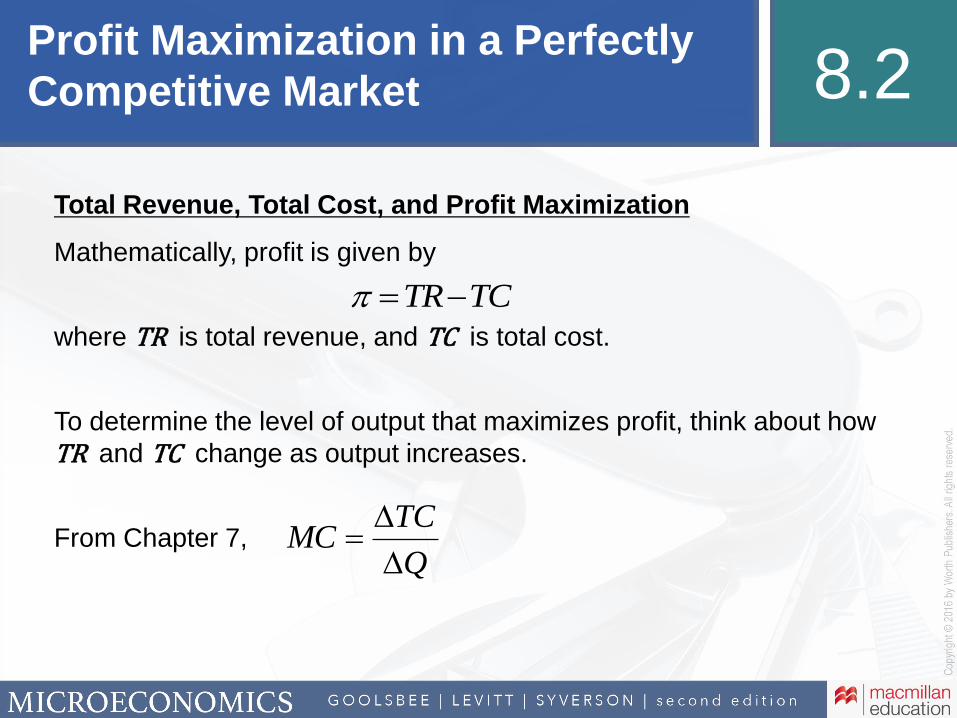
Total Revenue, Total Cost, and Profit Maximization

Mathematically, profit is given by

where TR is total revenue, and TC is total cost.

To determine the level of output that maximizes profit, think about how

TR and TC change as output increases.

From Chapter 7,

TCTR

Q

TCMC



Total Revenue, Total Cost, and Profit Maximization

Similarly, the additional revenue from selling one additional unit of output

is referred to as marginal revenue.

In perfect competition,

or, marginal revenue is simply equal to market price in a perfectly

competitive market structure.

• Recall the fundamental assumption of a perfectly elastic demand curve.

Q

TRMR

P

Q

QP

Q

QP

Q

TRMRPC



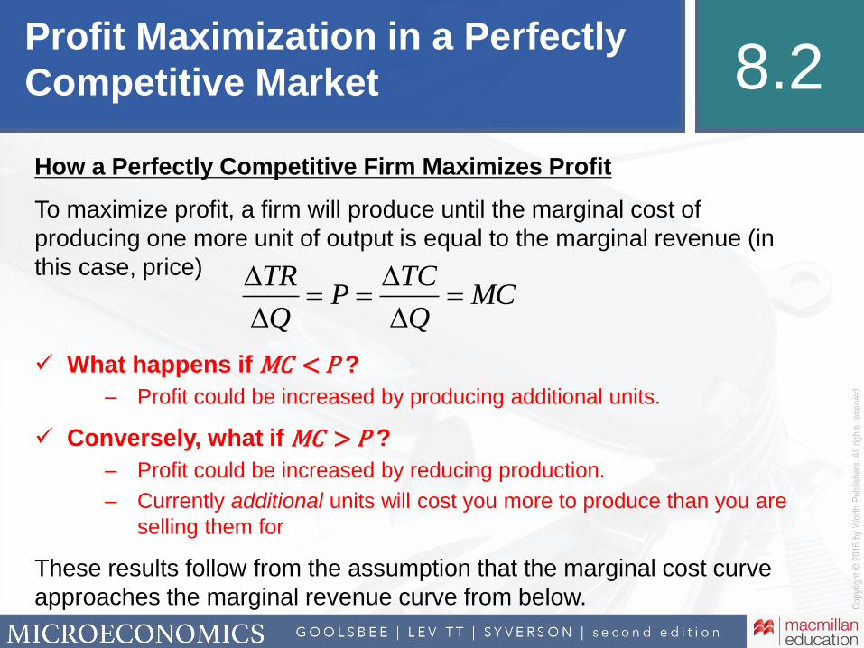
How a Perfectly Competitive Firm Maximizes Profit

To maximize profit, a firm will produce until the marginal cost of

producing one more unit of output is equal to the marginal revenue (in

this case, price)

What happens if MC < P ?

‒ Profit could be increased by producing additional units.

Conversely, what if MC > P ?

‒ Profit could be increased by reducing production.

‒ Currently additional units will cost you more to produce than you are

selling them for

These results follow from the assumption that the marginal cost curve

approaches the marginal revenue curve from below.

MCQ

TCP

Q

TR



Figure 8.3 Profit Maximization for a Perfectly Competitive

Firm Occurs Where MR = P = MC

Price & cost Marginal cost (MC )($/unit)

P2

P1 d = MR

P3

Quantity



Measuring a Firm’s Profit

To measure profit, simply subtract total cost from total revenue

Graphically, profit is measured by computing the area of a rectangle.

• Length = Q

• Height = the difference between P and ATC.

TCTR

QATCP

QATCQP



Figure 8.4 Measuring Profit

(a) Profit

(c) Negative Profit (Loss)(b) Zero Profit

Price& cost

($/unit)ATC aMCMC

ATC bATC *

P d = MRATC *

QuantityQ*

ATC c



Determining Whether to Shut Down

What happens if profit is negative? Should a firm shut down?

In the short run, the firm still has to pay its fixed costs. If the firm shuts

down, profits are given by

Alternatively, if the firm continues operating,

The difference is given by

In general, firms should remain open and operating in the short run as

long as revenue can cover variable costs, even if net profit is negative.

shut down TR TC TR FC VC

FCFC 00

operate TR TC TR FC VC

operate shut down TR VC



Figure 8.5 Deciding Whether to Operate or Shut Down in the

Short Run

PriceATC& cost MC

($/unit)

ATC* AVC

P* d = MR

AVC*

QuantityQ*

Loss

P > AVCContinueoperating




Continue operating if

where the * indicates the profit-maximizing (or loss-minimizing) quantity.

Shut down if

Continue operating as long as you cover your variable costs!

*or AVCPVCTR

*or AVCPVCTR

Perfect Competition in the

Short Run 8.3

A Firm’s Short-Run Supply Curve in a Perfectly Competitive Market

The supply curve (from Chapter 2) shows the quantity supplied at each

price.

Individual firms will choose to produce where price equals marginal cost;

the short-run supply curve is equal to the short-run marginal cost curve.

• One caveat: Only the portion of the short-run marginal cost curve above

the average variable cost (AVC) curve will be on the firm’s supply curve.

• Why?

‒ The firm won’t produce (or will shutdown) if P < AVC.


Short Run 8.3

Figure 8.6 The Perfectly Competitive Firm’s Short-Run

Supply Curve

Below average variable cost (AVC), the

firm will shut down (supply is zero).

Above average variable cost, the

marginal cost (MC) curve is the short-

run supply curve.

Quantity

AVC

Price & cost

($/unit)

ATC

Short-run supply curveMC


Short Run 8.3

The Short-Run Supply Curve for a Perfectly Competitive Industry

We know individual firms cannot affect market price in a perfectly

competitive industry.

Market price is instead determined by the interaction between market

supply and market demand.

Market supply is the horizontal sum of all individual firms’ supply curves.


Short Run 8.3

Producer Surplus for a Competitive Firm

Marginal cost slopes upward; therefore, in most circumstances some

output is being sold at a price above the cost of production.

Producer surplus is the sum of the differences between marginal cost

and the price of output at every level of output.

This is equivalent to the difference between total revenue and total

variable cost.

PS =TR-VC


Short Run 8.3

Figure 8.10 Producer Surplus for a Firm in Perfect

Competition

Price Price& cost & costMC MC

($/unit) ($/unit)

P d = MR P d = MR

Producer Producersurplus surplus

AVC AVCAVC * AVC *

Quantity QuantityQ* Q*

Both panelsare equivalent.

(a) Producer Surplus: Adding All of (b) Producer Surplus: Total Revenuethe Price-Marginal Cost Markups Minus Variable Costs


Short Run 8.3

Producer Surplus and Profit

Producer surplus is closely related to profit, but they are not the same

thing.

Firms will operate without making a profit, but they will shut down

if they are not making any producer surplus.

PS =TR-VC,

p =TR-VC -FC = PS -FC


Short Run 8.3

Producer Surplus for a Competitive Industry

Producer surplus for an entire industry is the sum of individual firms’

surplus.


Short Run 8.3

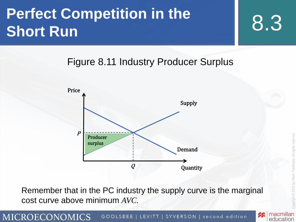
Figure 8.11 Industry Producer Surplus

Remember that in the PC industry the supply curve is the marginal

cost curve above minimum AVC.

Quantity

Demand

Price

Supply

PProducersurplus

Q

Perfectly Competitive

Industries in the Long Run8.4

The long run differs from the short run in a number of ways

1. In the short run, some costs are fixed; in the long run, all inputs, and

therefore costs—may be adjusted.

2. In the long run, firms can enter and exit freely in response to market

conditions.

3. The short-run supply curve is the portion of the short-run marginal

cost curve above the short-run average variable cost curve.

• In the long run, firms will not stay in business unless all costs can

be covered by revenue, therefore

‒ The long-run supply curve is the portion of the marginal cost

curve above the long-run average total cost curve.



Entry

Perfectly competitive markets are characterized by free entry

• The ability of a firm to enter an industry without encountering legal or

technical barriers.

What market conditions would have to exist for a firm to decide

to begin operation in a particular market?

‒ Firms will only enter if they see profit being made.

• Remember that the long-run ATC includes all costs, including

opportunity costs.

• If there are positive economic “profits,” new firms will enter.

When firms enter a market, the supply curve shifts outward.



Figure 8.14 Positive Long-Run Profit

PriceLMC LATC& cost

($/unit)

P1

LATC*P – LATC =

profit per unit

QuantityQ*



Figure 8.15 Entry of New Firms Increases Supply and

Lowers Equilibrium Price

Price ($)S1

S2

Entry

P1

P2

D

Quantity

If profits are positive in the long run, a lack of barriers to entry means more firms

will start producing.



Exit

Perfectly competitive markets are characterized by free exit.

• The ability of a firm to exit an industry without encountering legal or

technical barriers.

Opposite of entry, exit causes the industry supply curve to shift inward.

• Firms will exit (and market price will rise) until market price equals

minimum of the long-run average total cost curve.



Figure 8.16 Deriving the Long-Run Industry Supply Curve

(a) Industry (b) Representative Firm

Price ($) Price LMC& costS1

S2Taste ($/unit)change Entry LATC

P2 P2 d2 = MR2

SLRP1 P1 d1 = MR1

D2

D1

Quantity QuantityQ1 Q2



Adjustments Between Long-Run Equilibria

Describe the process of adjustment to a new market equilibrium in

response to the following:

An increase in demand: like the earlier graphs

• Existing firms enjoy positive economic profits in the short run because P >

LRATC.

• New firms eventually enter the market, supply shifts out, and price falls to

minimum long-run average total cost.

An increase in production costs:

• Some firms will experience negative economic profits in the short run.

• Eventually these firms will exit the industry and supply will shift inward,

driving up the market price until it is equal to long-run average total cost.



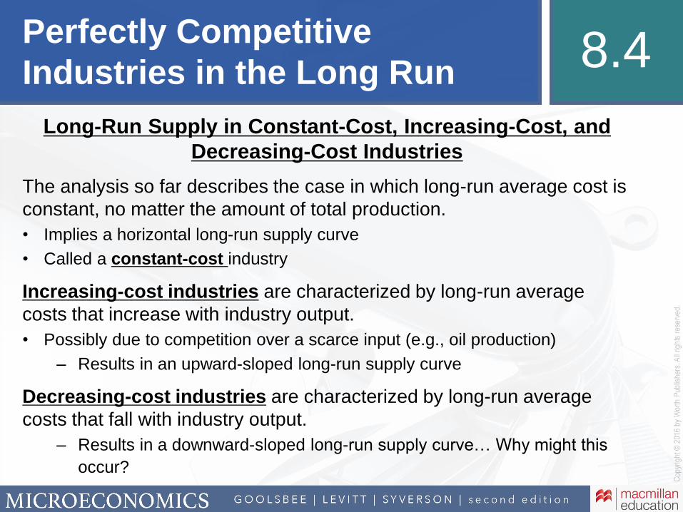
Long-Run Supply in Constant-Cost, Increasing-Cost, and

Decreasing-Cost Industries

The analysis so far describes the case in which long-run average cost is

constant, no matter the amount of total production.

• Implies a horizontal long-run supply curve

• Called a constant-cost industry

Increasing-cost industries are characterized by long-run average

costs that increase with industry output.

• Possibly due to competition over a scarce input (e.g., oil production)

‒ Results in an upward-sloped long-run supply curve

Decreasing-cost industries are characterized by long-run average

costs that fall with industry output.

‒ Results in a downward-sloped long-run supply curve… Why might this

occur?

Producer Surplus, Economic

Rents, and Economic Profits 8.5

Cost Differences and Economic Rent in Perfect Competition

In the long run, there is no potential for economic profit in a perfectly

competitive industry.

• Assumes producers have identical cost curves.

• However, some firms may be more efficient than others.

More efficient firms earn Economic Rent, or returns to specialized

inputs above what firms paid for them.

In a perfectly competitive market consisting of firms with different long-

run average cost curves:

• The long-run market price equals the minimum average total cost of the

highest-cost firm in the industry.

• The highest-cost firm makes zero profit and zero producer surplus.

Producer Surplus, Economic

Rents, and Economic Profits 8.5

Cost Differences and Economic Rent in Perfect Competition

Important distinction: Economic rent ≠ economic profit.

Economic rent is included in the opportunity costs associated with the

use of an input.

• An excellent manager or a trade secret would likely be useful in other

ventures as well.

• These “rents” often accrue to the more-productive-than-average inputs (e.g.,

salaries to the best managers).

Economic profit includes all opportunity costs.

Conclusion 8.6

Chapter 8 has analyzed the decisions facing firms in a perfectly

competitive industry:

• Characterized by few barriers to entry, a large number of firms

producing identical products, and firms that are price takers.

• Firms maximize profits by setting marginal cost equal to market price.

In the next chapters, we relax some of the assumptions of perfect

competition to include product differentiation, barriers to entry, and

other characteristics common to real-world markets.

In-text

figure it out

Assume that consumers view hair cuts as undifferentiated

among producers, and that there are hundreds of barbers in a

given market. The current market equilibrium price for a haircut

is $15. Bob’s Barbershop has a daily, short-run total cost given

by

with marginal cost

Answer the following questions:

a. How many haircuts should Bob prepare each day if his goal

is to maximize profits?

b. How much will he earn in profit each day?

25.0 QTC

QMC

In-text

figure it out

a. Bob is assumed to be operating in a perfectly competitive

market, so he will prepare returns up until the point that

marginal revenue (price) is equal to marginal cost.

b. To determine Bob’s daily profit, plug the profit-maximizing

quantity into the daily profit function.

1515)( QQMCPMR

20.5TR TC P Q Q

215 15 0.5(15)

$225 $112.5 per day

Additional

figure it out

Assume that consumers view tax preparation services as

undifferentiated among producers, and that there are hundreds

of companies offering tax preparation in a given market. The

current market equilibrium price is $120. Joe Audit’s Tax Service

has a daily, short-run total cost given by

with marginal cost


a. How many tax returns should Joe prepare each day if his

goal is to maximize profits?

b. How much will he earn in profit each day?

24100 QTC

QMC 8

Additional

figure it out

a. Joe is assumed to be operating in a perfectly competitive

market, so he will prepare returns up until the point that

marginal revenue (price) is equal to marginal cost.

b. To determine Joe’s daily profit, plug the profit-maximizing

quantity into the daily profit function.

158120 QQMCPMR

24100 QQPTCTR

)15(4100(15120 2

800$000,1800,1

In-text

figure it out

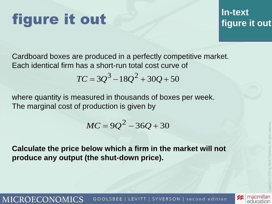
Cardboard boxes are produced in a perfectly competitive market.

Each identical firm has a short-run total cost curve of

where quantity is measured in thousands of boxes per week.

The marginal cost of production is given by

Calculate the price below which a firm in the market will not

produce any output (the shut-down price).

5030183 23 QQQTC

30369 2 QQMC

In-text

figure it out

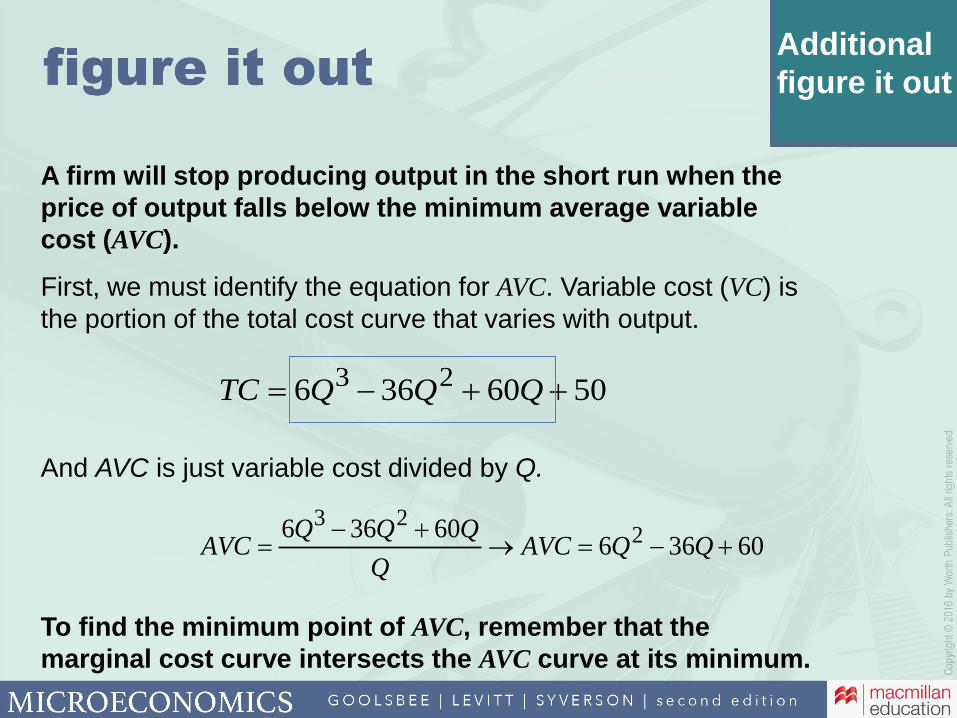
A firm will stop producing output in the short run when the

price of output falls below the minimum average variable

cost (AVC).

First, we must identify the equation for AVC. Variable cost (VC) is

the portion of the total cost curve that varies with output

And AVC is just variable cost divided by Q

To find the minimum point of AVC, remember that the

marginal cost curve intersects the AVC curve at its minimum.

5030183 23 QQQTC

3018330183 2

23

QQAVCQ

QQQAVC

In-text

figure it out

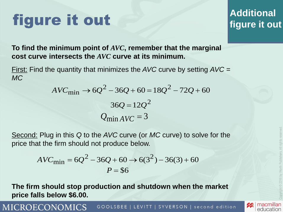
To find the minimum point of AVC, remember that the marginal

cost curve intersects the AVC curve at its minimum.

First: Find the quantity that minimizes the AVC curve by setting AVC =

MC.

Second: Plug in this Q the AVC (or MC curve) curve to solve for the

price that the firm should not produce below.

The firm should stop production and shutdown when the market

price falls below $3.00.

3036930183 22min QQQQAVC

2618 QQ

3min AVCQ

30)3(18)3(330183 22min QQAVC

3$P

Additional

figure it out

Cardboard boxes are produced in a perfectly competitive market.

Each identical firm has a short-run total cost curve of

where quantity is measured in thousands of boxes per week.

The marginal cost of production is given by

Calculate the price below which a firm in the market will not

produce any output (the shut-down price).

5060366 23 QQQTC

607218 2 QQMC

Additional

figure it out

A firm will stop producing output in the short run when the

price of output falls below the minimum average variable

cost (AVC).

First, we must identify the equation for AVC. Variable cost (VC) is

the portion of the total cost curve that varies with output.

And AVC is just variable cost divided by Q.

To find the minimum point of AVC, remember that the

marginal cost curve intersects the AVC curve at its minimum.

5060366 23 QQQTC

6036660366 2

23

QQAVCQ

QQQAVC

Additional

figure it out

To find the minimum point of AVC, remember that the marginal

cost curve intersects the AVC curve at its minimum.

First: Find the quantity that minimizes the AVC curve by setting AVC =

MC

Second: Plug in this Q to the AVC curve (or MC curve) to solve for the

price that the firm should not produce below.

The firm should stop production and shutdown when the market

price falls below $6.00.

60721860366 22min QQQQAVC

21236 QQ

3min AVCQ

60)3(36)3(660366 22min QQAVC

6$P

In-text

figure it out

Assume that the industry for pickles is perfectly competitive.

There are 150 producers. 100 of the firms are “high-cost,” with

short-run supply curves Qhc = 4P, while the others are “low-cost,”

with short-run supply curves Qlc = 6P. Quantities are measured in

jars and prices in dollars.


a. Derive the short-run industry supply curve for tortillas.

b. Assume the market demand curve for tortillas is given by

Qd = 6,000 – 300P. Find the market equilibrium price and

quantity.

c. At this price, how many pickles are produced by the high- and

low-cost firms, respectively?

d. Determine total industry surplus at the equilibrium.

In-text

figure it out

a. The short-run industry supply curve is found by

summing the firms’ supply curves:

b. The market equilibrium occurs where QS = QD

PPQQ DS 300000,6700

6$000,6000,1 PP

jarsQ

jarsQP

D

S

200,4)6(300000,6

200,4)6(7006$

PPPQS 7006504100

)(#)(# lclchchclchcS QFirmsQFirmsQQQ

In-text

figure it out

c. To determine how many jars of pickles are produced by the

high- and low-cost firms, respectively, plug P = $6 into each

type of producers’ supply curve.

d. Producer surplus (PS) is the area between the price line and

the industry supply curve.

Demand

Price

Supply

6

PS

12,600 Quantity

EE PQPS 2

1

600,12$

6$200,42

1

4 24 jarshcQ P

6 36 jarslcQ P

Additional

figure it out

Assume that the industry for flour tortillas in Denver is perfectly

competitive. There are 200 firms. 75 of the firms are “high-cost,”

with short-run supply curves Qhc = 5P, while the others are “low-

cost,” with short-run supply curves Qlc = 8P. Quantities are

measured in tortillas and prices in dollars.


a. Derive the short-run industry supply curve for tortillas.

b. Assume the market demand curve for tortillas is given by

QD = 10,000 – 625P. Find the market equilibrium price and

quantity.

c. At this price, how many dozens of tortillas are produced by

the high- and low-cost firms, respectively?

d. Determine total industry surplus at the equilibrium.

Additional

figure it out

a. The short-run industry supply curve is found by

summing the firms’ supply curves:

b. The market equilibrium occurs where QS = QD

75 5 125 8 1,375P P P

PPQQ DS 625000,101375

5$000,10000,2 PP

$5 1,375(5) 6,875 tortillas

10,000 625(5) 6,875 tortillas

S

D

P Q

Q

)(#)(# lclchchclchcS QFirmsQFirmsQQQ

Additional

figure it out

c. To determine how many tortillas are produced by the high- and

low-cost firms, respectively, plug P = $5 into each type of

producers’ supply curve.

d. Producer surplus (PS) is the area between the price line and

the industry supply curve.

Demand

Price

Supply

5

PS

6,825 Quantity

EE PQPS 2

1

50.187,17$

5$875,62

1

5 25 tortillashcQ P 8 40 tortillaslcQ P

In-text

figure it out

Suppose the market for cantaloupes is currently in long-run

equilibrium at a price of $3 per melon. A listeria outbreak in

cantaloupe crops leads to a sharp decline in the demand for

cantaloupe.


a. In the short run, what will happen to the price of cantaloupes?

Explain using a diagram.

b. In the short run, how will firms respond to the change in price

described in part (a)? What will happen to firms’ profits?

Explain using the same diagram.

c. Given the situation described in (b), what can we expect to

happen to the number of cantaloupe producers in the long

run?

d. What will the long run price of cantaloupes be?

In-text

figure it out

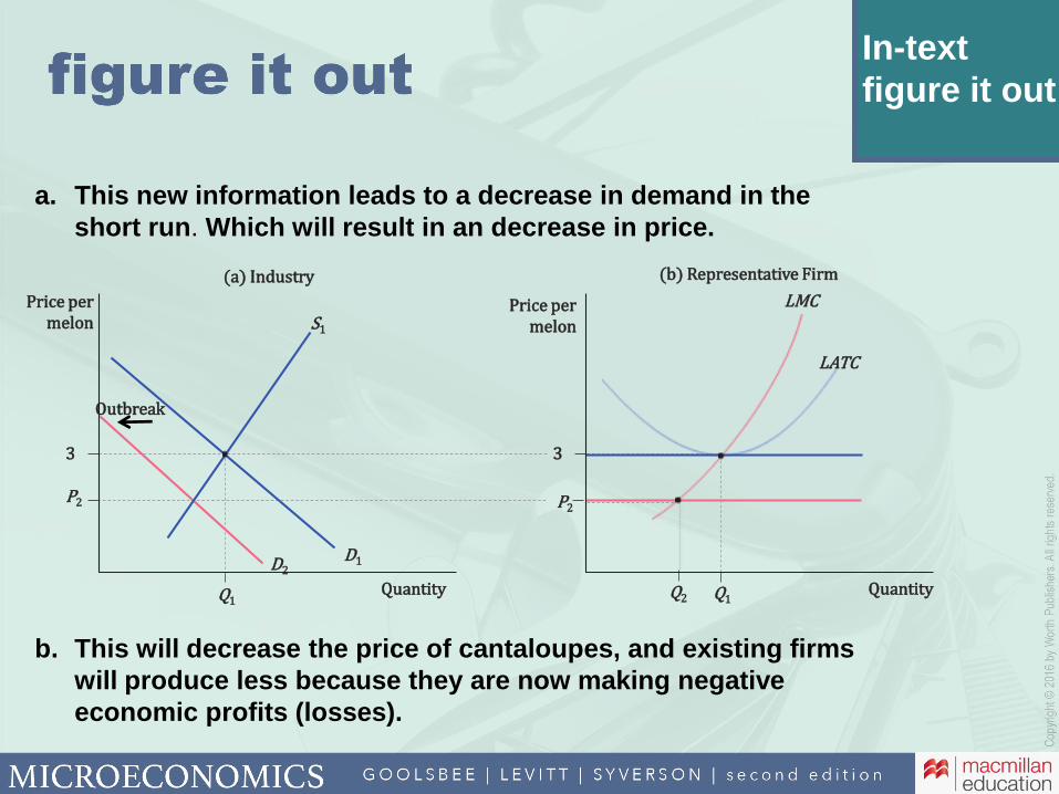
a. This new information leads to a decrease in demand in the

short run. Which will result in an decrease in price.

b. This will decrease the price of cantaloupes, and existing firms

will produce less because they are now making negative

economic profits (losses).

Price per melon


LMCS1

Outbreak

LATC

P2 P2

3 3

D2D1

Quantity QuantityQ1

Price per melon

Q2 Q1

In-text

figure it out

c. In the long-run, a number of producers will have losses

(at P2, Q*2) so some will exit the market.

d. In the long run the price of cantaloupes will rise back to the

initial equilibrium of $3 per melon as the reduction in supply

will drive price back to $3 where there are no more losses.

Price per melon


LMCS1

S2

OutbreakExit

LATC

P2 P2

SLRP1=$3 P1

D1

D2

Quantity Quantity

Price per melon

Q*1Q*2

D1 = MR1

D2 = MR2

Additional

figure it out

Suppose the market for the pain reliever, aspirin ,is currently in

long-run equilibrium at a price of $3 per bottle. New scientific

research is released that links aspirin with a reduced risk of heart

disease.


a. In the short run, what will happen to the price of aspirin?

Explain using a diagram.

b. In the short run, how will firms respond to the change in price

described in part (a)? What will happen to firms’ profits?

Explain using the same diagram.

c. Given the situation described in (b), what can we expect to

happen to the number of aspirin producers in the long run?

d. What will the long-run price of aspirin be?

Additional

figure it out

a. This new information will lead to an increase in demand in the

short run, which will result in an increase in price

b. This will increase the price of aspirin, and existing firms will

produce more because they are now making profits.

Price per bottle


LMCS1

Tastechange LATC

P2 P2

3 3

D2

D1

Quantity QuantityQ1

Price per bottle

Q*1 Q*

2

Additional

figure it out

c. In the long-run, the number of producers will rise because firms

see profits and enter the market.

d. In the long run the price of aspirin will fall back down to initial

equilibrium of $3 per bottle as more firms enter the market

seeking profit.

Price per bottle


LMCS1

S2Tastechange Entry LATC

P2 P2

SLRP1=3 P1

D2

D1

Quantity QuantityQ1 Q2

Price per bottle

Q*1 Q*2

Supply in a Competitive Market - University of Southern ...ebayrak/teaching/LECTURES/303/week 8...

Documents

Transcript of Supply in a Competitive Market - University of Southern ...ebayrak/teaching/LECTURES/303/week 8...