www.sciencemag.org/cgi/content/full/science.1228380/DC1

Supplementary Materials for

Kepler-47: A Transiting Circumbinary Multiplanet System

Jerome A. Orosz,* William F. Welsh, Joshua A. Carter, Daniel C. Fabrycky, William D. Cochran, Michael Endl, Eric B. Ford, Nader Haghighipour, Phillip J. MacQueen, Tsevi Mazeh, Roberto Sanchis-Ojeda, Donald R. Short, Guillermo Torres, Eric Agol, Lars A. Buchhave, Laurance R. Doyle, Howard Isaacson, Jack J. Lissauer, Geoffrey W. Marcy,

Avi Shporer, Gur Windmiller, Thomas Barclay, Alan P. Boss, Bruce D. Clarke, Jonathan Fortney, John C. Geary, Matthew J. Holman, Daniel Huber, Jon M. Jenkins, Karen Kinemuchi, Ethan Kruse, Darin Ragozzine, Dimitar Sasselov, Martin Still, Peter Tenenbaum, Kamal Uddin, Joshua N. Winn, David G. Koch, William J. Borucki

*To whom correspondence should be addressed. E-mail: orosz@sciences.sdsu.edu

Published 28 August 2012 on Science Express DOI: 10.1126/science.1228380

This PDF file includes:

Materials and Methods Supplementary Text Figs. S1 to S25 Tables S1 to S9 References (25–59)

Supporting Online Material (SOM)

We provide additional details regarding the detection and characterization of Kepler-47in this supplement.§1.1 gives alternate designations and other information forKepler-47.§1.2 discusses the Kepler data preparation and detrending.§1.3 discusses how the rota-tional period of the primary star is derived. §1.4 discusses the ground-based spectroscopicobservations.§1.5 describes how the effective temperature, gravity, and metallicity of theprimary were measured. §1.6 gives an overview of how the times of mid-eclipse for theprimary and secondary eclipses were measured.§1.7 discusses the effects of star-spots onthe measurement of the eclipse times and other parameters.§1.8 presents measurementsof the transit times and the detection of a transit event possibly due to a third planet. §1.9gives a full discussion of the photometric-dynamical model. §1.10 presents a discussionof independent light curve modeling done with the ELC code.§1.11 discusses how upperlimits on the masses of the planets were derived.§1.12 considers the long-term stability ofthe planetary orbits. §1.13 gives a comparison of the stellar properties with evolutionarymodels.§1.14 presents details of the habitable zone in Kepler-47.

1 Materials and Methods

1.1 Alternate designations, celestial coordinates, and apparent magnitudes

Kepler-47 appears in the Kepler Input Catalog (25,KIC) as KIC 10020423. Other designationsinclude Kepler Object of Interest KOI-3154 and 2MASS J19411149+4655136. The J2000 ce-lestial coordinates given in the KIC areα = 19h41m11.s501, δ = +4655′13.′′69, and the appar-ent magnitudes arer = 15.126 andKp = 15.178.

1.2 Kepler data preparation and detrending

In this study we make use of data from Kepler Quarters Q1 through Q12 (May, 2009 throughlate March, 2012). We used the “simple aperture photometry”(SAP) provided by the Keplerpipeline and available at the Mikulski Archive for Space Telescopes (MAST). The Kepler SAPlight curves show instrumental trends (26), so further processing is necessary. The detrendingmust be done for each Quarter separately since the object appears on a different detector module.The amount of detrending needed depends on the specific task.When modeling the eclipses andtransits, a fairly aggressive detrending is used where boththe instrumental trends and the spotmodulations are removed. In this case, the eclipses and transits are masked out, and a high ordercubic spline is fit to short segments whose end points are usually defined by gaps in the datacollection due to monthly data downloads, rolls between Quarters, or spacecraft safe modes.The segments are normalized to the spline fits, and the segments are reassembled. The SAPlight curves and the detrended light curve with the spot modulation removed are shown in Fig.

1

S1. Other tasks such as spot modeling require much less aggressive detrending, in which caselow-order polynomials are used to stitch together different segments across the Quarters.

The time difference between the last Q12 observation and thefirst Q1 observation is 1050.51days. During that interval, Kepler was collecting data 92.55% of the time, and 44389 cadencesout of the 47580 in total were flagged as good (SAPQUALITY=0), for a duty cycle of 86.34%.Not all observations with SAPQUALITY>0 are necessarily useless, depending on the purpose,so the 86.34% duty cycle is a lower limit.

1.3 Rotational period from star-spot induced stellar variations

Fig. S2 shows closer-in views of the light curves from Q1, Q5,and Q9. A modulation of up to3% in the out-of-eclipse regions due to star spots rotating into and out of view is evident. Thismodulation has a period that is close to, but not exactly equal to the eclipse (e.g. orbital) pe-riod. Fig. S3 depicts the autocorrelation of the cleaned detrended light curve, after the primaryand secondary eclipses were removed and replaced by the value of the mean light curve with atypical random noise. The autocorrelation reveals clear modulation with a period of about 7.8days. Presumably, the clock behind the modulation is the stellar rotation of the primary, whichhas brightness variation due to inhomogeneous distribution of stellar spots (as the primary stardominates the light in the Kepler bandpass, we assume it is the source of the modulation). Toobtain a more precise value of the stellar rotation we measured the lags of the first 12 peaks ofthe autocorrelation and fitted them with a straight line as shown in Fig. S4. From the slope of thefitted line we derived a value of7.775± 0.022 days as our best value for the stellar rotation pe-riod. This period is slightly longer than the orbital periodof 7.448 days. It is interesting to notethat the transition between synchronized and unsynchronized binaries for pre-main sequenceand young stars appears between 7 and 8 days, as depicted by (27).

1.4 Spectroscopic observations

We observed Kepler-47 four times with the High-Resolution-Spectrograph (28, HRS) at theHobby-Eberly Telescope (HET). Spectra with a resolving power ofR = 30, 000 were obtainedon UT 2012, April 23, May 18 & 20 and June 5. We used the “600g5822” setting of HRS thatdelivers a spectrum from 4814 to 6793A. The data were reduced with our own HRS reductionscript using standard IRAF routines. We selected a total exposure of 3600 seconds per spectrum(divided into three sub-exposures of 1200 seconds each to facilitate cosmic-ray removal). Thesignal-to-noise (S/N) levels of the HRS spectra range from 30:1 to 55:1 at 5500A, dependingon seeing conditions. Adjacent to every visit to Kepler-47 we also observed the Kepler fieldstandard star HD 182488 to be used for the radial velocity determination.

In addition to the HET observations, we observed Kepler-47 six times using the Tull Coudespectrograph (29) at the Harlan J. Smith 2.7m telescope (HJST). The data were obtained withour standard instrumental setup that covers the a wavelength range of 3760-10,200A and usesa 1.2 arcsecond slit that yields a resolving power ofR = 60, 000. We obtained data during the

2

nights of UT 2012, May 1, 2, 4-6 and on June 26. Exposure times ranged from 3600 to 4800seconds (again divided in 1200 second sub-exposures) and the S/N is typically around 14:1 at5500A. Each of these nights we also observed HD 182488 to serve as aradial velocity standard.The data were reduced with our own reduction scripts using standard IRAF routines. Aftersome experimentation, it was discovered that better measurements of the radial velocities wereobtained from spectra that did not have the sky background subtracted.

An additional spectrum of Kepler-47 was obtained using the 10 m Keck 1 telescope and theHIRES spectrograph (30). The spectra were collected using the standard planet search setupand reduction (31). The resolving power isR = 60, 000 at 5500A. Sky subtraction, using the“C2 decker” was implemented with a slit that projects to0.87 × 14.0 arcsec on the sky. Thewavelength calibrations were made using Thorium-Argon lamp spectra.

The radial velocities of Kepler-47 were measured using the “broadening function” technique(32). The broadening functions (BFs) are rotational broadeningkernels, where the centroid ofthe peak yields the Doppler shift and where the width of the peak is a measure of the rotationalbroadening. The BF analysis is often better suited for measuring radial velocities of binary starsin cases where the velocity difference between the two starsis small compared to the spectralresolution. A high quality spectrum of a slowly rotating star is needed for the BF analysis,and for this purpose we used observations of HD182488 (spectral type G8V) taken with eachtelescope+instrument combination. The derived radial velocities are insensitive to the precisespectral type of the template, as similar radial velocitiesare found when using templates of earlyG to late K. The adopted template radial velocity was−21.508 km s−1 (33).

We prepared the spectra for the BF analysis by normalizing each echelle order to the localcontinuum using cubic splines, trimming the low signal-to-noise ends of each order, and merg-ing the orders by interpolating to a log-linear wavelength scale. The wavelength ranges usedfor the final BF analysis was 4830-5770A for the HET spectra and 5138-5509A for the HJSTspectra. Fig. S5 shows example BFs from HET and HJST spectra. The spectrum is single-lined,as only one peak is evident in the BFs from the HET. Some simple simulations were performed,and non-detection of a second star in the HET spectra indicates the secondary star is>∼10 timesfainter than the primary star, consistent with the expectations based on the eclipse depths, wherea flux ratio of∼ 1/176 is expected. In the case of the HJST, two peaks are apparent. However,one of the peaks is due to the sky background since it is stationary in velocity, and changesstrength relative to the other. The FWHM of the BF peaks were consistent with the instrumen-tal broadening, which indicates the rotational velocity ofthe primary is at best only marginallyresolved.

Gaussian functions were fit to the BF peaks to determine the relative Doppler shifts. Theappropriate barycentric velocity corrections were applied and the contribution of the templateradial velocity was removed, thereby placing the radial velocities on the standard IAU radialvelocity scale defined by (33) and (34). The Keck HIRES pipeline automatically produces radialmeasurements for single stars on the IAU scale, accurate to 0.1 km s−1 or better (34). Havingestablished Kepler-47 as a single-lined binary, we simply adopted the pipeline measurement.The radial velocity measurements for all 11 observations are given in Table S1.

3

1.5 Spectroscopic parameters

The effective temperatureTeff , surface gravitylog g, the metallicity [m/H], and the rotationalvelocityVrot sin i of the primary were measured using the Stellar Parameter Classification (SPC)code (35). SPC uses a cross-correlation analysis against a large grid of model spectra in thewavelength region 5050 to 5360A. Since all of the absorption lines in this region are used, theSPC analysis is ideal for spectra with low signal-to-noise.The first three HET observations werecombined to yield a spectrum with a signal-to-noise ratio of≈ 116 in the order containing theMg b features near 5169A (the fourth HET observation had relatively high sky contaminationand was not used). The derived spectroscopic parameters aregiven in Table S2.

1.6 Stellar eclipse times and corrections

The times of mid-eclipse for the primary and secondary eclipses in Kepler-47 were measuredusing the technique described in (7). For completeness we give most of the details here as well.Given an initial linear ephemeris and an initial estimate ofthe eclipse widths, the data near theeclipses were isolated and locally detrended using a cubic polynomial with the eclipses maskedout. The detrended data were then folded on the linear ephemeris and an eclipse template wasmade by fitting a cubic Hermite spline. The Piecewise Cubic Hermite Spline (PCHS) modeltemplate was then iteratively cross-correlated with each individual eclipse event to produce ameasurement of the time at mid-eclipse. After each iteration, a new PCHS model was producedby using the latest measured times to fold the data. Fig. S6 shows the folded eclipse profiles andthe final PCHS models. The fits are generally good, although there is increased scatter near themiddle of the primary eclipse, presumably due to the effectsof star spots. Table S3 gives theeclipse times. The cycle numbers for the secondary eclipse are not exactly half integers becausethe orbit is eccentric.

The eclipse times were fitted with a linear ephemeris and the Observed minus Computed (O-C) residual times were calculated and are shown in Fig. S7. Forthe primary, there are coherentdeviations of up to two minutes. While not strictly periodic,there is a quasiperiod of≈ 178days seen in a periodogram (Fig. S8). This modulation is mostlikely a beat frequency betweenthe stellar rotation and the binary motion, similar to what is observed for Kepler-17 (20). Ifthe secondary passes in front of a big spot during the primaryeclipse, the spot anomaly willintroduce a shift on the eclipse timing since the projected stellar disk of the primary on thesky will no longer have a symmetric surface brightness distribution. The shift of the eclipsetime will depend on the size and position of the spot and the position on the eclipse chord. Along-lasting spot will introduce shifts in consecutive eclipses, but the shift will change withtime since the spot will be at a different position on the eclipse chord at each eclipse. Morespecifically for this system, a spot with a period of rotationof 7.775 days will effectively recedeon the transit chord360(7.4484 d − 7.775 d)/7.4484 d = −15.79 each eclipse. In order tocome back to the exact same position, and hence complete a full cycle in the O-C diagram,(360/15.79)Porb = 22.8Porb = 170 days will be needed, which is close to the period of the

4

observed signal. In reality, the spots also change with timeand may also drift in latitude overtime, so the signal near the beat frequency is blurred somewhat.

There is a correlation between the O-C residual time of the primary eclipse and the localslope of the out-of-eclipse portions of the SAP light curve during the eclipse, as shown in Fig.S9. A large negative slope in the light curve surrounding an eclipse indicates a dark spot isrotating into view. The “center of light” of the primary willbe shifted to the opposite side ofthe stellar disk, resulting in a slightly later time of mid-eclipse. Likewise, a large positive slopesurrounding an eclipse indicates a dark spot is rotating outof view, which results in a slightlyearlier time of mid-eclipse. Finally, when the slope is nearzero, the spots are centered on thestellar disk, and no change in the eclipse time is seen. A linear function was fitted to the data inFig. S9, and the times of primary eclipse were corrected. TheO-C diagram resulting from thesecorrected times (Fig. S7) has much less scatter. No periodicities are evident (Fig. S8).

The best-fitting ephemerides for the corrected primary eclipse times and the secondaryeclipse times are

PA = 7.44837605± 0.00000050 d Kepler-47 primaryPB = 7.44838227± 0.00000342 d Kepler-47 secondary

T0(A) = 2, 454, 963.24539± 0.000041 Kepler-47 primaryT0(B) = 2, 454, 959.426986± 0.000277 Kepler-47 secondary

The difference between the primary and secondary periods is0.52 ± 0.30 seconds, with thesecondary period being longer.

1.7 The effect of star-spots on the eclipses: possible biases and spin-orbitalignment.

Star-spots cause the light curve to exhibit modulations that can be used to measure the rotationperiod of the primary star. Star-spots can also affect the determination of certain system param-eters. It has been shown that there is a correlation between the eclipse timing variations andthe local slope of the stellar flux variations at the times of the eclipses. In order to confirm thatstar-spots are the main cause of the eclipse timing variations, and to evaluate their impact onour ability to measure the size of the secondary star, we attempt to model the effect of spots onindividual eclipses (21,36,37).

The data from each primary eclipse are isolated by keeping only 3 hours of observationsbefore and after the eclipse. The out-of-eclipse part of each dataset is then fitted with a linearfunction. The fit is subtracted from the data, then the data are normalized so the out-of-eclipseflux is equal to unity. The detrended eclipse light curves arefolded with a linear ephemeris, andthis folded light curve is fitted with a standard model for light loss due to a dark body passing infront of a limb darkened star (38). This no-spot model has only four free parameters: squaredradius ratio(RB/RA)

2, impact parameterb, normalized semimajor axis for the secondary orbitRA/aB, and a linear limb darkening coefficientu1.

5

The effect spots have on individual primary eclipses is manifest in two ways: the depth ofeach eclipse changes since it is measured relative to the changing stellar flux, and the shapeof each eclipse is distorted which leads to a shift in the measured mid-eclipse time. Visualinspection of the eclipse residuals shows that this last effect can be well-modeled in most casesby adding just one large star-spot on the surface of the primary star. Since the rotation of thestar happens on a longer time-scale than the eclipse itself,we held the position of the star-spotfixed during each individual eclipse. The latitude of the spots cannot be well constrained withsingle eclipse events, so we fix the position of the spot so that the center of the secondary startrajectory intersects the center of the spot. Our spot modeladds five additional parameters:three parameters describe the spot itself – its angular radius, the flux contrast (related to thespot temperature), and the position along the eclipse chord. The fourth parameter is the out-of-eclipse flux, which corrects for the depth variations. Finally, the time of mid-eclipse is free. Weset up a pixilated model of the star with a circular spot, in which the flux is calculated as thesurface integral of the intensity of the visible hemisphereof the star.

The best-fitting model for several consecutive eclipses is compared with a no-spot modelin Fig. S10, showing how the model captures the essential effect of spots on the eclipses. Forevery eclipse we obtained a new eclipse time, and fitted a linear ephemeris to these times. Thescatter was found to be substantially reduced from the initial timings (see Fig. S7, upper panel),by a factor of 30%, which shows that indeed the scatter is due to spots. The improvement onthe scatter is similar to the one obtained through the local slope correction, so this serves as agood consistency check.

Our model also estimates the fraction of the star covered by spots at the time of each eclipse.This quantity is not very precise, but can help us estimate the effect of spots on the measurementof the eclipse depth and hence the radius ratioRA/RB. We divide the square of the radius ratiofrom the spot model by each observed local out-of-eclipse flux to mimic the apparent depth thatone would obtain by fitting each eclipse individually. The results are plotted in Fig. S11, whereone can clearly see how the depth of each eclipse changes withtime. The variations seem tohave a time-scale similar to the uncorrected eclipse timingvariations, which is expected sincethe scatter in both are due to spots. A variation with the observing season is also apparent,which is a clear indication that there are different levels of Quarterly contamination. With theseeclipse depths we can estimate the inferred secondary star radiusRB from each eclipse, using afixedRA from Table 1 (see Fig. S11). The values obtained do not have a large scatter, and theyall agree within1σ with the value obtained from the photometric-dynamical model fit. Thusthe correction to the secondary star radius because of the presence of spots is not significant,although a slightly smaller radius is favored.

We can also use these spot models to gain information about the obliquity of the sys-tem (18–21, 39). In Fig. S10 we can clearly see how the spot model shows that aspot ismoving backwards with each eclipse, which means that the spot trajectory is contained withinthe boundaries of the eclipse chord. This backwards movement makes it seem as if the star isrotating backwards (retrograde) very slowly, but this is simply a stroboscopic alias effect. Thespot appears to move backwards because the star’s rotation period is slightly longer than the

6

orbital period.If we assume that the entire trajectory of a spot is containedon the part of the primary

star eclipsed by the secondary star then we can estimate the obliquity of the system (18) tobe smaller thanarctan(RB/RA) ≈ 20. The obliquity is likely to be smaller since we havedetected more than 10 spots receding with different velocities, and these different velocitiescould be due to spots at different latitudes exhibiting differential rotation. We note that theobliquity of this target will be very hard to measure with theRossiter-McLaughlin effect (40)due to its faintness, so additional investigation of its spots might be the preferred method tofurther constrain the obliquity.

In principle, we can use the spectroscopicVrot sin i together with an estimated rotation pe-riod and size of the primary star to obtain information on theinclination of the primary star. Thespectroscopic observedVrot sin i = 4.1 ± 0.5 km s−1, while the inferredVrot = 2πRA/Prot =6.3 ± 0.2 km s−1. This would imply a highly inclined star (is ≈ 40). Note, however, thatthe measured value of the rotational velocity is below the resolution of the spectra, so its valueshould be treated with caution. In addition, differential rotation can make it harder to comparethe surface integrated projected rotational velocityVrot sin i to the equatorial rotational velocity2πRA/Prot (39).

1.8 Transit times for the inner and outer planet and the search for addi-tional transits

All of the transits of the outer planet and about half of the transits of the inner planet are evi-dent in the SAP light curves before any detrending. The rest became visible when the data arecarefully detrended. A symmetric polynomial “U-function”template with an adjustable widthand depth was used to estimate the times of mid-transit and their durations. A cubic polynomialwas used to detrend each transit using five different duration windows around the transit, and thebest-fitting one was adopted. The fits for each transit were iterated to determine the best-fittingtime of mid-transit and the duration. This method worked well in some cases and failed toconverge in other cases. In cases where the convergence failed, the time was estimated using aninteractive plotting program, and an uncertainty of 30, 60 or 90 minutes was assigned based onthe judged quality of the transit. Table S4 gives the measured times and durations and their un-certainties, and the corresponding model times and durations. We note that the measured timesand the durations were only used to establish starting models for the photometric-dynamicalmodels described below. The actual (detrended) light curvewas modeled directly.

One “orphan” transit occurring about 12 hours after a transit of planet b was noticed inthe Q12 data (Fig. S12). This transit cannot be accounted forby either the inner or the outerplanet (the intervals between the nearest transits are 0.5 days and 127 days, respectively). Toestimate the significance of the orphan event, a model consisting of two Gaussians was fit to thesegment of the detrended light curve shown in Fig. S12, whichcontains 103 data points. Theuncertainties on each point were scaled to giveχ2

ν = 1 for 96 degrees of freedom. The Gaussianin the model at the location of the orphan was replaced by the background level of 1.0 and the

7

resultingχ2 value increased to 205.5, giving a formal significance of∼ 10.5σ.No other orphan transits with a significance of> 3σ were found using visual searches. An

automated search algorithm, dubbed the “Quasi-periodic Automated Transit Search” (QATS)was also used to search for additional transits. The QATS algorithm can allow for unequal timeintervals between the transit events. For a given trial period for a potential planet, the expectedtransit duration at each time in the light curve is computed using a circular orbit for the planet.The data are corrected for the different transit durations and shifted to a common phase toincrease the signal-to-noise (the correction for the different widths is quite good, provided theplanet’s orbit is nearly circular). A “periodogram” is constructed by plotting the significanceversus the trial period. QATS detected the inner planet at high significance. UnfortunatelyQATS is very sensitive to detrending errors for longer periods, and in fact did not detect theouter planet. No additional planets with periods shorter than 150 days were detected at thesignificance level of the inner planet.

Although the overall duty cycle of the data collection by Kepler is quite high, a non-trivialamount of the light curve is occupied by the stellar eclipses, which in the case of Kepler-47 is≈ 3−6 times more than it is for Kepler-16, 34, 35, and 38. Although one could in principle findtransits during primary and secondary eclipses, in Kepler-47 this is extremely difficult owingto the effects of star-spots. The primary and secondary eclipse durations together are 0.014 inorbital phase, which is 0.104 days. A combined total of 256 primary and secondary eclipseswere observed, giving a total of 26.62 days lost for the purposes of transit searches, loweringthe duty cycle to 83.8%.

Finally, if the transit is due to another planet in the Kepler-47 system, its radius would be≈ 4.5 Earth radii. Without more transit events, it is nearly impossible to determine what theorbital period of such a planet would be. If its orbit is more inclined relative to the other planets,it would not necessarily transit the stars near each conjunction. In addition, if there is precessionof the orbit, it is possible for sequences of transits to comeand go over long time scales. Thus,the orphan transit could in principle belong to a planet in between the inner and outer one, inspite of the lack of other observed transits.

1.9 Photometric-dynamical model

We modeled the Kepler light curve of Kepler-47 using a dynamical model to predict the motionsof the planets and stars, and a eclipse/transit model to predict the light curve.

1.9.1 Description of the model

The “photometric-dynamical model” refers to the model thatwas used to fit the Kepler photom-etry. This model is analogous to that described in the analyses of KOI-126 (13), Kepler-16 (6),Kepler-34 and Kepler-35 (7), Kepler-36 (41), and Kepler-38 (8).

Four bodies were involved in this problem; however, the planets’ gravitational interactionwith the stars and with each other was determined to be observationally negligible. We therefore

8

assumed the planets to be massless in our model. The motion ofthe stellar binary was Keple-rian and could be predicted analytically. The planets were modeled as orbiting in the two-bodypotential of the stars. The motion of each planet was determined via a three-body numericalintegration. This integration utilized a hierarchical (orJacobian) coordinate system. In thissystem,rb (rc) is the position of Planet b (Planet c) relative to the center-of-mass of the stellarbinary (which corresponds to the barycenter in this approximation), andrEB is the position ofStar B relative to Star A. The computations are performed in aCartesian system, although itis convenient to expressrb (rc) andrEB and their time derivatives in terms of osculating Kep-lerian orbital elements: instantaneous period, eccentricity, argument of pericenter, inclination,longitude of the ascending node, and time of barycentric conjunction: Pb,c,EB, eb,c,EB, ib,c,EB,ωb,c,EB, Ωb,c,EB, Tb,c,EB, respectively. We note that these parameters do not necessarily reflectobservables in the light curve; the unique three-body effects make these parameters functionsof time (and we refer to these coordinates as “osculating”).

The accelerations of the three bodies are determined from Newton’s equations of motion,which depend onrb (rc), rEB and the masses (42,43). For the purpose of reporting the massesand radii in Solar units, we assumedGMSun = 2.959122 × 10−4 AU3 day−2 andRSun =0.00465116 AU. We used a Bulirsch-Stoer algorithm (44) to integrate the coupled first-orderdifferential equations forrb,EB andrb,EB.

The spatial coordinates of all four bodies at each observed time are calculated and used asinputs to model the light curve. The computed flux was the sum of the fluxes assigned to StarA, Star B, and a seasonal (being the four “seasons” of the Kepler spacecraft orientation) sourceof “third light,” minus any missing flux due to eclipses or transits (only planetary transits acrossStar A were computed, those across Star B are not significant in the Kepler data). The lossof light due to eclipses was calculated as follows. All objects were assumed to be spherical.The sum of the fluxes of Star A and Star B was normalized to unityand the flux of Star B wasspecified relative to that of Star A. The radial brightness profiles of Star A and Star B weremodeled with a linear limb-darkening law, i.e.,I(r)/I(0) = 1−u1(1−

√1− r2) wherer is the

projected distance from the center of a given star, normalized to its radius, andu is the linearlimb-darkening parameter. The limb darkening coefficient of Star B was fixed (tou = 0.5);letting it vary freely resulted in a negligible change to final parameter posterior.

The radial velocity of Star A was computed from the time derivative of the position of StarA along the line of sight (analytically, in this case) and compared to the radial velocity data.

The continuous model is integrated over a 29.4 minutes interval centered on each long ca-dence sample before being compared to the long cadence Kepler data.

1.9.2 Local detrending of Kepler data

The Kepler light curve (“SAPFLUX” from the standard fits product) for Kepler-47, spanningtwelve Quarters, is reduced to only those data within 0.5–1 day of any primary or secondaryeclipse or any transit of either planet. As noted above, somedata are missing as a result ofobservation breaks during Quarterly data transfers or spacecraft safe modes.

9

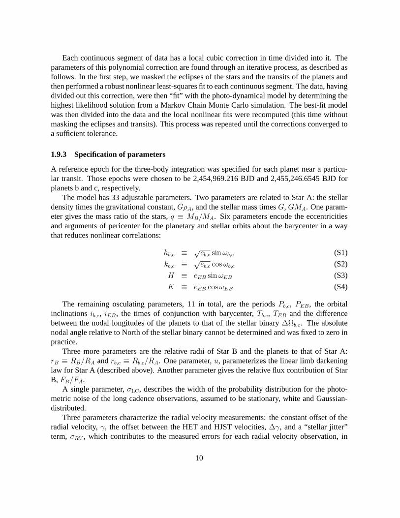
Each continuous segment of data has a local cubic correctionin time divided into it. Theparameters of this polynomial correction are found throughan iterative process, as described asfollows. In the first step, we masked the eclipses of the starsand the transits of the planets andthen performed a robust nonlinear least-squares fit to each continuous segment. The data, havingdivided out this correction, were then “fit” with the photo-dynamical model by determining thehighest likelihood solution from a Markov Chain Monte Carlo simulation. The best-fit modelwas then divided into the data and the local nonlinear fits were recomputed (this time withoutmasking the eclipses and transits). This process was repeated until the corrections converged toa sufficient tolerance.

1.9.3 Specification of parameters

A reference epoch for the three-body integration was specified for each planet near a particu-lar transit. Those epochs were chosen to be 2,454,969.216 BJDand 2,455,246.6545 BJD forplanets b and c, respectively.

The model has 33 adjustable parameters. Two parameters are related to Star A: the stellardensity times the gravitational constant,GρA, and the stellar mass timesG, GMA. One param-eter gives the mass ratio of the stars,q ≡ MB/MA. Six parameters encode the eccentricitiesand arguments of pericenter for the planetary and stellar orbits about the barycenter in a waythat reduces nonlinear correlations:

hb,c ≡ √eb,c sinωb,c (S1)

kb,c ≡ √eb,c cosωb,c (S2)

H ≡ eEB sinωEB (S3)

K ≡ eEB cosωEB (S4)

The remaining osculating parameters, 11 in total, are the periods Pb,c, PEB, the orbitalinclinationsib,c, iEB, the times of conjunction with barycenter,Tb,c, TEB and the differencebetween the nodal longitudes of the planets to that of the stellar binary∆Ωb,c. The absolutenodal angle relative to North of the stellar binary cannot bedetermined and was fixed to zero inpractice.

Three more parameters are the relative radii of Star B and theplanets to that of Star A:rB ≡ RB/RA andrb,c ≡ Rb,c/RA. One parameter,u, parameterizes the linear limb darkeninglaw for Star A (described above). Another parameter gives the relative flux contribution of StarB, FB/FA.

A single parameter,σLC, describes the width of the probability distribution for the photo-metric noise of the long cadence observations, assumed to bestationary, white and Gaussian-distributed.

Three parameters characterize the radial velocity measurements: the constant offset of theradial velocity,γ, the offset between the HET and HJST velocities,∆γ, and a “stellar jitter”term, σRV , which contributes to the measured errors for each radial velocity observation, in

10

quadrature. Because only one Keck observation was made, thisradial velocity could not beoffset to match the HET and HJST velocities in a sensible way,and therefore was omitted in themodeling.

Additionally, we specify 4 more parameters describing the relative extra flux summed inthe aperture. The four parameters specify the constant extra flux in each Kepler “season.” TheKepler spacecraft is in one of four orientations during a year; a constant level of “third light” isassumed for all Quarters sharing a common season.

1.9.4 Priors and likelihood

We assumed uniform priors for all 33 parameters. For the eccentricity parameters, this corre-sponds to uniform priors ineb,c andωb,c, but a prior that scales aseEB for the stellar eccentricity.This eccentricity is sufficiently determined that this non-uniform prior does not dominate theposterior distribution.

The likelihoodL of a given set of parameters was taken to be the product of likelihoodsbased on the photometric data and radial velocity data:

L ∝ σ−NLC

LC exp

−NLC∑

i

(∆FLCi )2

2σ2LC

(S5)

×NRV∏

j

(

σ2

j + σ2

RV

)−1/2exp

− (∆Vj)2

2(

σ2j + σ2

RV

)

where∆F LCi is the ith photometric data residual,σLC is the width parameter describing the

photometric noise of the long cadence data,∆Vj is thejth radial velocity residual,σj is theuncertainty in thejth radial velocity measurement andσRV is the stellar jitter term added inquadrature with theσj.

1.9.5 Best-fit model

We determined the best-fit model by maximizing the likelihood. The maximum likelihood solu-tion was found by finding the highest likelihood in a large draw from the posterior as simulatedwith a Markov Chain Monte Carlo simulation as described below.Fig. S13 shows 18 transitsof the inner planet, and Fig. S14 shows the residuals (observed data minus the model). With afew exceptions, there are no strong patterns in the residuals. Fig. S15 shows the model fits andthe residuals for the outer planet. There are no patterns evident in the residuals. The residualsfor the fits to the primary eclipses are shown in Fig. S16 and the residuals for the fits to thesecondary eclipses are shown in Fig. S17. Spot crossing events are evident in many of the pri-mary eclipses. Fig. S18 shows the radial velocity measurements and the best-fitting model andthe residuals of the fit. Generally the absolute value of the radial velocity residuals is less thanabout 200 m s−1.

11

The photometric noise parameter,σLC , has a best-fit value ofσLC = 629.5 ppm. For com-parison, the root-mean-square deviation of the best-fit residuals is626.9 ppm. This is similarto the expected noise in the light curve of 635 ppm as estimated using an on-line tool providedby the Kepler Guest Observer Office1, where we used an apparent magnitude of Kp=15.18 and20 pixels in the aperture. For thisσLC , theχ2-metric for the photometric data isχ2 = 10576with 10629 degrees of freedom. If we fail to include planet b in our model (by setting its ra-dius to zero), theχ2 increases by∆χ2 = 343.4. If we ignore planet c, theχ2 increases by∆χ2 = 248.2.

The stellar jitter parameter,σRV , has a best-fit value ofσRV = 0.31 km s−1. The value ofχ2 for the radial velocity data alone isχ2 = 8.85 for the 10 radial velocity observations.

Fig. S19 shows schematic diagrams of the Kepler-47 orbits. The projected orbits of planetsb and c cross the projected disk of the primary, and so transits of both planets across the primaryoccur, as do occultations of both planets by star A. The former events are observed, whereasthe latter events are not observable given the noise level. On the other hand, owing to itssmall radius, the projected disk of star B does not intersectthe projected orbits of the planets,and as such no transits of star B or occultations due to star B occur for the best-fitting orbitalconfiguration. Due to the uncertainties in the relative nodal angles, transits of the planets acrossstar B might occur for a subset of the acceptable solutions. However, even if transits across starB did occur, the expected transit depth would be∼ 30 times weaker than the transits across theprimary, and would not be observable in the light curve giventhe noise level.

1.9.6 Parameter estimation methodology

We explored the parameter space and estimated the posteriorparameter distribution with a Dif-ferential Evolution Markov Chain Monte Carlo (DE-MCMC) algorithm (45).

We generated a population of 100 chains and evolved them through approximately 200,000generations. The initial parameter states of the 100 chainswere randomly selected from an over-dispersed region in parameter space bounding the final posterior distribution. The first 10% ofthe links in each individual Markov chain were clipped, and the resulting chains were concate-nated to form a single Markov chain, after having confirmed that each chain had convergedaccording to the standard criteria.

The parameter values and derived values reported in Tables S5 and S6 beside the best-fitvalues (see above), were found by computing the 15.8%, 50%, 84.2% levels of the cumulativedistribution of the marginalized posterior for each parameter. Figure S20 shows two-parameterjoint distributions between all parameters. This figure is meant to highlight the qualitativefeatures of the posterior as opposed to providing quantitative ranges. The numbers in that figurecorrespond to the model parameters in Table S5 with the same number listed as in the firstcolumn, if available.

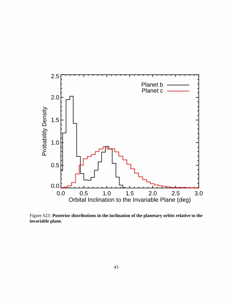
Figures S21 and S22 show the posterior distribution in the eccentricity and argument ofpericenter planes The distribution of the three-dimensional inclination between the planets’

1http://keplergo.arc.nasa.gov/CalibrationSN.shtml

12

orbits and the invariable plane is shown in Figure S23.

1.9.7 Predicted ephemerides and transit parameters

Tables S7 and S8 provide the predicted times of transit, impact parameters, normalized transitvelocities and durations over 7 years, starting with KeplerQuarter Q13.

1.10 ELC light curve models

Although the secondary star is not detected spectroscopically, its temperature can be estimatedusing the temperature of the primary derived using SPC, and the temperature ratio derivedfrom modeling the eclipses. In order to find the temperature ratio, and to have an independentcheck on the results from the photometric-dynamical model,we modeled the light and velocitycurves using the Eclipsing Light Curve (ELC) code (46) with its genetic algorithm and MonteCarlo Markov Chain optimizers. The free parameters include the temperature ratioTB/TA, theprimary’s limb darkening parametersxA andyA for the quadratic limb darkening law [I(µ) =I0(1 − x(1 − µ) − y(1 − µ)2)], the orbital parameters (e, ω, i), and the fractional radiiRA/aandRB/a. The stellar masses and the orbital period were held fixed at the values derived fromthe photometric-dynamical model discussed above.

In ELC, the shapes of the stars are computed using a “Roche” potential modified to accountfor nonsynchronous rotation and eccentric orbits (47,48). Given the mass ratio and the fractionalradii, the volumes of each star are found by numerical integration. The effective radius of eachstar is taken to be the radius of a sphere with the same volume as the equipotential surface. Inthe case of Kepler-47, the stars are very nearly spherical. For the primary at periastron, the ratioof the polar radius to its effective radius is 0.99988, and the ratio of the radius along the lineof centers to the effective radius is 1.00007. The amplitudeof the out-of-eclipse modulation inthe light curve due to ellipsoidal variations, reflection, and Doppler boosting is on the order of400 ppm, which is≈ 75 times smaller than the modulation due to star-spots. Thus the use ofspherical stars in the photometric-dynamical model is a very good approximation.

Since the numerical integrations are very CPU intensive, ELChas a fast “analytic” modewhere the equations given in (49) are used. The normalized light curve was divided into 41 seg-ments containing two or three pairs of primary and secondaryeclipses. These segments weremodeled separately in order to help assess the systematic errors associated with the changingstar-spots and the changes in the contamination from Quarter to Quarter. For each fitting pa-rameter, we computed the mean of the best-fitting values and the standard deviation. Table S9gives the mean values and standard deviations, which we adopt as1σ errors.

Based on the temperature of the primary derived from the SPC analysis, and the temperatureratio found from the ELC models, we derive a temperature of3357± 100 K for the secondary.

13

1.11 Upper limits on planetary masses

Upper limits on the masses of the planets can be placed separately as follows. The mass ofthe inner planet is best constrained by the lack of eclipse timing variations due to gravitationalperturbations from that planet. The planet will induce short-term eclipse timing variations witha period equal to the planet’s period. It will also cause precession of the binary. Over the time-scale of a few years, the binary precession will cause a slight change in the phase differencebetween the primary and secondary eclipses, which can be observed as a slight difference be-tween the primary and secondary eclipse periods. Numericalsimulations showed that in thiscase the stronger upper limit comes from the lack of short-term eclipse timing variations. A gridof masses for the inner planet was used, and equations of motion for a three body system wereintegrated, holding the orbital parameters of the binary attheir best-fitting values (the natureof the perturbations on the binary are insensitive to anything except the planet’s mass). Theperiod and epoch of the binary was found, and the predicted times of eclipse were comparedto the measured times. Theχ2 value changes smoothly with the planet’s mass, and going toχ2 = χ2

min+ 9 gives a3σ upper limit of 2.7 Jupiter masses for the uncorrected eclipse times

and 2.0 Jupiter masses for the eclipse times corrected for the effect of star-spots. We adopt thelatter value as the3σ upper limit on the mass of the inner planet.

The mass of the outer planet was best constrained by light travel time (LTT) effects. We fitan LTT orbit to the corrected eclipse times, using a period of303.13 days and constraining theeccentricity to bee < 0.2. While no convincing signal is seen at that period, the best-fittingorbit formally has a semiamplitude of3.84 ± 1.84 seconds. Given the total mass of the binaryand the period of the outer planet, we find a3σ upper mass limit of 28 Jupiter masses.

1.12 Stability of orbits and limits on eccentricity

We carried out an extensive study of the dynamics of the system and its long-term stability.The orbits of the two planets were integrated, numerically,for different values of their massesand orbital eccentricities. To determine an upper limit forthe eccentricity of planet c, we heldconstant all orbital elements at their best-fit values and integrated the system varying the eccen-tricity of this planet. Results indicated that the system maintained stability for at least 100 Myrand forec < 0.6. An examination of the semimajor axis, eccentricity, and orbital inclination ofeach planet during the course of the integrations showed that the variations of these quantitieswere negligibly small, supporting the idea that the two planets do not disturb each other’s orbits.The results stayed unchanged when the masses of the two planets were increased to 0.21 and0.63 Jupiter masses, roughly ten times their plausible values based on the empirical mass-radiusrelations (14,15).

Both the photometric-dynamical model and stability simulations used a Newtonian 4-bodynumerical integrator. A more physical model would include the precession of the binary due togeneral relativity (GR) and the tidal and rotational bulges.Expressions for the rate of precessiondue to these effects (50) show that GR dominates, and it would cause a full periastronrotation

14

in ∼ 6700 years. In the current observations, such precession would cause the period of primaryand secondary eclipse to differ fractionally by∼ 10−7, whereas the uncertainty of this quantityis 4.6 × 10−7. The GR precession period is much longer than the periastronperiod of theplanets – e.g., numerical integrations of planet c showing a∼ 560 year precession cycle dueto the effective quadrupolar gravitational potential of the binary – so it has little dynamicalimportance. Therefore GR and other precession effects are neither detectable nor significantlychange our assessment of stability, so GR has little dynamical importance.

1.13 Comparison with stellar evolution models

The reasonably precise absolute dimensions determined forthe stars in Kepler-47 (4–5% rel-ative errors for the masses, and 1.8% for the radii) offer an opportunity to compare the mea-surements with models of stellar evolution. This is of particular interest for the late M-dwarfsecondary, given that low-mass stars have shown discrepancies with theory in the sense thatthey are generally larger and cooler than predicted. These anomalies are believed to be due tostellar activity (51,52).

In Fig. S24 we compare the measurements for the primary star with a stellar evolutiontrack from the Yonsei-Yale series (53, 54), interpolated to the exact mass we measure. Themetallicity of this model is set by our spectroscopic determination of [Fe/H] = −0.25, wherewe assume the iron abundance tracks the metallicity measurement from SPC. The model isconsistent with the observations to within less than2σ, and the small difference may be dueeither to slightly biased spectroscopic parameters (temperature and metallicity) or a slightlyoverestimated mass for the primary star. As a check, we produced a photometric estimateof the temperature using available photometry from the KIC and empirical color-temperaturecalibrations along with the reddening listed in the KIC. The result suggests a value closer to5900 K than 5600 K, although we consider this evidence to be somewhat circumstantial andhighly dependent on reddening. We confirmed that the level ofagreement between theoryand observation is independent of the adopted model physicsby comparing the primary starparameters with BaSTI stellar evolutionary tracks (55), which yielded similar results as theYonsei-Yale models.

In Fig. S25 we compare the measurements for both components against models from theDartmouth series (56), which incorporate physical ingredients (equation of state, non-greyboundary conditions) more appropriate for low-mass stars.We find the radius of the secondaryof Kepler-47 to be consistent with these models, which wouldbe an exception to the generaltrend mentioned above, although the mass error is large enough (∼4%) that the conclusion isnot as strong as in other cases. Its temperature, however, islower than predicted for a star of thismass by about 200 K. This deviation is in the same direction asseen for other low-mass stars.Because the secondary is so faint, we have no information on its activity level. Age estimatesfor the system from this figure and the previous one are somewhat conflicting, and only allowus to say that Kepler-47 is very roughly of solar age.

15

1.14 Details of habitable zone

To determine the insolation limits of the habitable zone forKepler-47 c, we follow the relationsgiven by (24) that include the stellar temperature as well as luminosity. The temperature termaccounts for the different relative amount of infrared flux to total flux, which is important foratmospheric heating. We use the criteria of a runaway greenhouse effect for the inner boundaryand the maximum greenhouse effect for a cloud-free carbon dioxide atmosphere for the outerboundary. This is more conservative than the “recent Venus”and “early Mars” criteria, but lessconservative than the “water loss” and “first carbon dioxidecondensation” criteria (24). Thesecondary star emits only 1.7% as much energy as the primary star (and only 0.58% in theKepler bandpass), so its contribution is neglected. The resulting insolation limits are shown asthe dotted lines in Figure 3 (main text). The relations givenin (57), i.e. a cloud-free atmosphereyield nearly identical limits.

The average insolation for Kepler-47 c for a circular orbit is 87% of the Sun-Earth insolation,and varies by∼ 9% peak-to-peak. For an eccentricity of 0.2 the mean insolation is 89% andvaries from 59% to 144% of the Sun-Earth value; for an eccentricity of 0.4, the mean is 96%and varies from 43% to 261%. Even in this latter case, which isruled out at the 95% confidencelevel by the photometric-dynamical model, the mean is less than the Sun-Earth value, and it isthe mean insolation that is most relevant for habitability (58). Thus for all allowed eccentricities,Kepler-47 c lies in the habitable zone.

Because the primary star dominates the system both in luminosity and mass (so the primarystar remains near the barycenter), the variation in insolation is relatively small for a circularplanetary orbit. This is seen in the upper left panel of Figure 3, where the variations are causedby the 7.4-day orbit of the primary star. For large eccentricities, the variation in insolation aredominated by the non-circular orbit of the planet.

It must be stressed that the habitable zone is defined such that liquid water could persist fora biologically significant time period on an Earth-like planet (i.e. with a terrestrial CO2/H2O/N2

atmosphere, plate tectonics, etc.), and the formulations of (17, 24, 57) explicitly assume suchconditions. For Kepler-47 c these conditions are not met. Nevertheless, the main point is thatKepler-47 c receives approximately the same amount of energy from its stars that the Earthreceives from the Sun.

While it neglects most atmospheric physics, the equilibriumtemperatureTeq of the planetis still a useful characterization. Assuming that the entire surface of the planet radiates isother-mally (i.e. the stellar insolation is efficiently advected around the planet), and for a Bond albedoof AB=0.7, appropriate for a Neptune-size planet and 1 Sun-Earthinsolation (59), a value ofTeq ∼ 200 K is found for eccentricities from 0.0 to 0.3. ForAB=0.34, corresponding to thealbedos of Jupiter and Saturn,Teq ∼ 243K. For an Earth-like albedo of 0.29, which is appropri-ate for a habitable-zone planet,Teq ∼ 247 K. The greenhouse effect will lead to temperaturesat the 1-bar pressure level that are higher by several tens ofdegrees.

16

17

References and Notes

1. D. G. Koch et al., Kepler mission design, realized photometric performance, and early science.

Astrophys. J. 713, L79 (2010). doi:10.1088/2041-8205/713/2/L79

2. W. J. Borucki et al., Kepler planet-detection mission: Introduction and first results. Science

327, 977 (2010). doi:10.1126/science.1185402 Medline

3. N. M. Batalha et al., Planetary candidates observed by Kepler, III: Analysis of the first 16

months of data. Astrophys. J. Suppl. Ser. submitted, arXiv1202.5852 (2012).

4. A. Prša et al., Kepler eclipsing binary stars. I. catalog and principal characterization of 1879

eclipsing binaries in the first data release. Astron. J. 141, 83 (2011). doi:10.1088/0004-

6256/141/3/83

5. R. W. Slawson et al., Kepler eclipsing binary stars. II. 2165 eclipsing binaries in the second

data release. Astron. J. 142, 160 (2011). doi:10.1088/0004-6256/142/5/160

6. L. R. Doyle et al., Kepler-16: A transiting circumbinary planet. Science 333, 1602 (2011).

doi:10.1126/science.1210923 Medline

7. W. F. Welsh et al., Transiting circumbinary planets Kepler-34 b and Kepler-35 b. Nature 481,

475 (2012). doi:10.1038/nature10768 Medline

8. J. A. Orosz, W. F. Welsh, J. A. Carter, E. Brugamyer, L. A., Buchhave, et al., The Neptune-

sized circumbinary planet Kepler-38b. Astrophys. J. in press, arXiv:1208.3712 (2012).

9. S. Meschiari, Circumbinary planet formation in the Kepler-16 system. I. N-body simulations.

Astrophys. J. 752, 71 (2012). doi:10.1088/0004-637X/752/1/71

10. S.-J. Paardekooper, Z. M. Leinhardt, P. Thébault, C. Baruteau, How not to build Tatooine:

The difficulty of in situ formation of circumbinary planets Kepler 16b, Kepler 34b, and

Kepler 35b. Astrophys. J. 754, L16 (2012). doi:10.1088/2041-8205/754/1/L16

11. T. Borkovits, B. Érdi, E. Forgács-Dajka, T. Kovács, On the detectability of long period

perturbations in close hierarchical triple stellar systems. Astron. Astrophys. 398, 1091

(2003). doi:10.1051/0004-6361:20021688

12. See the Supplementary Materials on Science Online.

13. J. A. Carter et al., KOI-126: A triply eclipsing hierarchical triple with two low-mass stars.

Science 331, 562 (2011). doi:10.1126/science.1201274 Medline

14. S. R. Kane, D. M. Gelino, The habitable zone gallery. Publ. Astron. Soc. Pac. 124, 323

(2012). doi:10.1086/665271

18

15. J. J. Lissauer et al., Architecture and dynamics of Kepler’s candidate multiple transiting

planet systems. Astrophys. J. Suppl. Ser. 197, 8 (2011). doi:10.1088/0067-0049/197/1/8

16. M. J. Holman, P. A. Wiegert, Long-term stability of planets in binary systems. Astron. J.

117, 621 (1999). doi:10.1086/300695

17. J. F. Kasting, D. P. Whitmire, R. T. Reynolds, Habitable zones around main sequence stars.

Icarus 101, 108 (1993). doi:10.1006/icar.1993.1010 Medline

18. R. Sanchis-Ojeda et al., Starspots and spin-orbit alignment in the WASP-4 exoplanetary

system. Astrophys. J. 733, 127 (2011). doi:10.1088/0004-637X/733/2/127

19. P. A. Nutzman, D. C. Fabrycky, J. J. Fortney, Using star spots to measure the spin-orbit

alignment of transiting planets. Astrophys. J. 740, L10 (2011). doi:10.1088/2041-

8205/740/1/L10

20. J. M. Désert et al., The hot-Jupiter Kepler-17b: Discovery, obliquity from stroboscopic

starspots, and atmospheric characterization. Astrophys. J. Suppl. Ser. 197, 14 (2011).

doi:10.1088/0067-0049/197/1/14

21. R. Sanchis-Ojeda et al., Alignment of the stellar spin with the orbits of a three-planet system.

Nature 487, 449 (2012). doi:10.1038/nature11301 Medline

22. A. Pierens, R. P. Nelson, On the formation and migration of giant planets in circumbinary

discs. Astron. Astrophys. 483, 633 (2008). doi:10.1051/0004-6361:200809453

23. A. N. Youdin, K. M. Kratter, S. J. Kenyon, Circumbinary Chaos: Using Pluto’s Newest

Moon to Constrain the Masses of Nix and Hydra. Astrophys. J. 755, 17 (2012).

doi:10.1088/0004-637X/755/1/17

24. D. R. Underwood, B. W. Jones, P. N. Sleep, The evolution of habitable zones during stellar

lifetimes and its implications on the search for extraterrestrial life. Int. J. Astrobiol. 2, 289

(2003). doi:10.1017/S1473550404001715

25. T. M. Brown, D. W. Latham, M. E. Everett, G. A. Esquerdo, Kepler input catalog:

Photometric calibration and stellar classification. Astron. J. 142, 112 (2011).

doi:10.1088/0004-6256/142/4/112

26. K. Kinemuchi et al., Demystifying Kepler data: A primer for systematic artifact mitigation.

Publ. Astron. Soc. Pac. in press, arXiv1207.3093 (2012).

27. T. Mazeh, in Observational Evidence for Tidal Interaction in Close Binary Systems, eds. M.-

J. Goupil & J.-P. Zahn, EAS Publications Series, vol. 29, p. 29 (2008).

28. R. G. Tull, High-resolution fiber-coupled spectrograph of the Hobby-Eberly Telescope. Proc.

Soc. Photo-opt. Inst. Eng. 3355, 387 (1998).

19

29. R. G. Tull, P. J. MacQueen, C. Sneden, D. L. Lambert, The high-resolution crossdispersed

echelle white-pupil spectrometer of the McDonald Observatory 2.7-m telescope. Publ.

Astron. Soc. Pac. 107, 251 (1995). doi:10.1086/133548

30. S. S. Vogt et al., HIRES: The highresolution echelle spectrometer on the Keck 10-m

Telescope. Proc. Soc. Photo-opt. Inst. Eng. 2198, 362 (1994).

31. G. W. Marcy et al., Exoplanet properties from Lick, Keck and AAT. Phys. Scr. T130,

014001 (2008). doi:10.1088/0031-8949/2008/T130/014001

32. S. M. Rucinski, Spectral-line broadening functions of WUMa-type binaries. I - AW UMa.

Astron. J. 104, 1968 (1992). doi:10.1086/116372

33. D. L. Nidever, G. W. Marcy, R. P. Butler, D. A. Fischer, S. S. Vogt, Radial velocities for 889

late-type stars. Astrophys. J. Suppl. Ser. 141, 503 (2002). doi:10.1086/340570

34. C. Chubak, G. W. Marcy, D. A. Fischer, A. W. Howard, H. Isaacson, H., et al., Precise radial

velocities of 2046 nearby FGKM stars and 131 standards. Astrophys. J. Supp. Ser.

submitted, arXiv:1207.6212v1 (2012).

35. L. A. Buchhave et al., An abundance of small exoplanets around stars with a wide range of

metallicities. Nature 486, 375 (2012). Medline

36. S. Czesla, K. F. Huber, U. Wolter, S. Schröter, J. H. M. M. Schmitt, How stellar activity

affects the size estimates of extrasolar planets. Astron. Astrophys. 505, 1277 (2009).

doi:10.1051/0004-6361/200912454

37. J. A. Carter et al., The transit light curve project. XIII. Sixteen transits of the Super-Earth GJ

1214b. Astrophys. J. 730, 82 (2011). doi:10.1088/0004-637X/730/2/82

38. K. Mandel, E. Agol, Analytic light curves for planetary transit searches. Astrophys. J. 580,

L171 (2002). doi:10.1086/345520

39. T. Hirano et al., Measurements of stellar inclinations for Kepler planet candidates. Astrophys.

J. 756, 66 (2012). doi:10.1088/0004-637X/756/1/66

40. J. N. Winn et al., Measurement of spin-orbit alignment in an extrasolar planetary system.

Astrophys. J. 631, 1215 (2005). doi:10.1086/432571

41. J. A. Carter et al., Kepler-36: A pair of planets with neighboring orbits and dissimilar

densities. Science 337, 556 (2012). doi:10.1126/science.1223269 Medline

42. S. Soderhjelm, Third-order and tidal effects in the stellar three-body problem. Astron.

Astrophys. 141, 232 (1984).

43. R. A. Mardling, D. N. C. Lin, Calculating the tidal, spin, and dynamical evolution of

extrasolar planetary systems. Astrophys. J. 573, 829 (2002). doi:10.1086/340752

20

44. W. H. Press, S. A. Teukolsky, W. T. Vetterling, B. P. Flannery, Numerical recipes in C++:

the art of scientific computing. (Cambridge University Press, Cambridge, 2002).

45. C. J. F. Ter Braak, A Markov Chain Monte Carlo version of the genetic algorithm

Differential Evolution: Easy Bayesian computing for real parameter spaces. Stat.

Comput. 16, 239 (2006). doi:10.1007/s11222-006-8769-1

46. J. A. Orosz, P. H. Hauschildt, The use of the NextGen model atmospheres for cool giants in a

light curve synthesis code. Astron. Astrophys. 364, 265 (2000).

47. Y. Avni, The eclipse duration of the X-ray pulsar 3U 0900-40. Astrophys. J. 209, 574 (1976).

doi:10.1086/154752

48. R. E. Wilson, Eccentric orbit generalization and simultaneous solution of binary star light

and velocity curves. Astrophys. J. 234, 1054 (1979). doi:10.1086/157588

49. A. Giménez, Equations for the analysis of the light curves of extra-solar planetary transits.

Astron. Astrophys. 450, 1231 (2006). doi:10.1051/0004-6361:20054445

50. D. Fabrycky, Non-Keplerian dynamics of exoplanets. in Exoplanets. ed. S. Seager,

University of Arizona Press, p. 217 (2011).

51. M. López-Morales, On the correlation between the magnetic activity levels, metallicities, and

radii of low-mass stars. Astrophys. J. 660, 732 (2007). doi:10.1086/513142

52. G. Torres, J. Andersen, A. Giménez, Accurate masses and radii of normal stars: Modern

results and applications. Astron. Astrophys. Rev. 18, 67 (2010). doi:10.1007/s00159-009-

0025-1

53. S. Yi et al., Toward better age estimates for stellar populations: The Y2 isochrones for solar

mixture. Astrophys. J. Suppl. Ser. 136, 417 (2001). doi:10.1086/321795

54. P. Demarque, J. H. Woo, Y.-C. Kim, S. K. Yi, Y2 Isochrones with an improved core

overshoot treatment. Astrophys. J. Suppl. Ser. 155, 667 (2004). doi:10.1086/424966

55. A. Pietrinferni, S. Cassisi, M. Salaris, F. Castelli, A large stellar evolution database for

population synthesis studies. I. scaled solar models and isochrones. Astrophys. J. 612,

168 (2004). doi:10.1086/422498

56. A. Dotter et al., The Dartmouth stellar evolution database. Astrophys. J. Suppl. Ser. 178, 89

(2008). doi:10.1086/589654

57. F. Selsis et al., Habitable planets around the star Gliese 581? Astron. Astrophys. 476, 1373

(2007). doi:10.1051/0004-6361:20078091

58. D. M. Williams, D. Pollard, Earth-like worlds on eccentric orbits: Excursions beyond the

habitable zone. Int. J. Astrobiol. 1, 61 (2002). doi:10.1017/S1473550402001064

21

59. K. L. Cahoy, M. S. Marley, J. J. Fortney, Exoplanet albedo spectra and colors as a function

of planet phase, separation, and metallicity. Astrophys. J. 724, 189 (2010).

doi:10.1088/0004-637X/724/1/189

Figure S1:SAP and detrended light curves. Top: The SAP light curves of Kepler-47 areshown. The colors denote the season and hence the spacecraftorientation where black is for Q1,Q5, and Q9, red is for Q2, Q6, and Q10, green is for Q3, Q7, and Q11, and blue is for Q4, Q8,and Q12. Bottom: The normalized and detrended light curve with the spot modulation removedis shown. Fifteen primary eclipses and thirteen secondary eclipses were missed during monthlydata downloads, spacecraft rolls between Quarters, spacecraft safe modes, and interruptionscaused by solar flares.

22

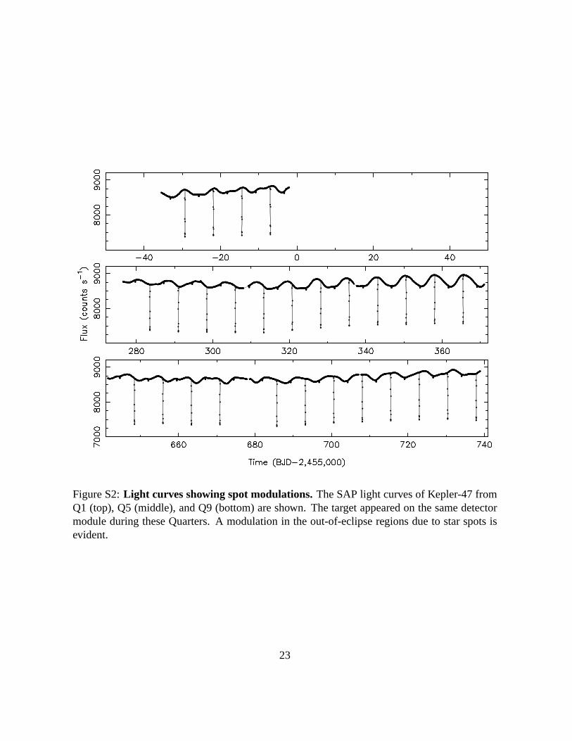
Figure S2:Light curves showing spot modulations.The SAP light curves of Kepler-47 fromQ1 (top), Q5 (middle), and Q9 (bottom) are shown. The target appeared on the same detectormodule during these Quarters. A modulation in the out-of-eclipse regions due to star spots isevident.

23

0 10 20 30 40 50 60 70 80 90 100−0.8

−0.6

−0.4

−0.2

0

0.2

0.4

0.6

0.8

1

Lag [days]

Aut

o co

rr

Figure S3:The autocorrelation function of the cleaned light curve with the eclipses re-moved.

0 2 4 6 8 10 120

10

20

30

40

50

60

70

80

90

100

Peak number

Lag

[day

s]

slope: 7.775 ± 0.022 [day]

Figure S4:The measured lag versus the peak number in the autocorrelation function. Themeasured lag of the peaks in the autocorrelation function displayed in Fig. S3 is shown. Thedashed line is a linear fit to these points. The slope of7.775 ± 0.022 days is taken to be therotation period of the primary star.

24

Figure S5: Representative broadening functions. Broadening functions (BFs) from theHET+HRS (left) and the HJST+Tull spectrograph (right) are shown. The solid lines are thebest-fitting Gaussians. The smaller peak in the HJST BF is due to the sky background. In allcases, the BF peak due to the sky was resolved from the object BF peak.

25

Figure S6: Mean primary and secondary eclipse profiles. The observed profiles for theprimary eclipse (dots, left panel) and the secondary eclipse (dots, right panel) arrived at afteran iterative process. The Piecewise Cubic Hermit Spline (PCHS) models are shown as the solidlines. The increased scatter in the middle of the primary eclipse is most likely due to the effectsof star spots.

26

Figure S7:Observed minus computed curves for the stellar eclipses.Top: The Observedminus Computed (O-C) residual times of the primary eclipses. Coherent deviations of nearlytwo minutes are seen, with a quasiperiod of≈ 178 days. Middle: The O-C times of the primaryafter correction for the effects of star spots. No periodicities or trends are evident. Bottom: TheO-C times for the secondary star. Note the change in the vertical scale. The error bars are notshown for clarity. The scatter is much larger, and no periodicities or trends are seen.

27

Figure S8:Lomb-Scargle periodograms of O-C curves.Top: A Lomb-Scargle periodogramof the O-Cs of the primary eclipses, before any corrections for star spots have been applied.The peak power occurs at a period of 179.2 days (dashed line).The expected beat period of≈ 170 days is indicated by the dotted line. Bottom: A Lomb-Scargle periodogram of theprimary eclipse O-Cs after a correction for the effects of star spots has been applied. There isno significant power at any period.

28

Figure S9:The correlation of residual O-C time and local slope near primary eclipse.Thedependence of the primary eclipse O-C times on the local SAP light curve slope is shown. Aclear correlation is seen. The best-fitting line has a coefficient of correlation ofr = −0.80.

29

−4 −2 0 2 4Time from the mid−eclipse [hours]

0.5

0.6

0.7

0.8

0.9

1.0

Rel

ativ

e flu

x +

con

stan

t

Cyc # 60

Cyc # 61

Cyc # 62

Cyc # 63

Cyc # 64

No spot modelOne spot model

−4 −2 0 2 4Time from the mid−eclipse [hours]

−0.06

−0.04

−0.02

0.00

0.02

O−

C R

esid

uals

+ c

onst

ant Cyc # 60

Cyc # 61

Cyc # 62

Cyc # 63

Cyc # 64 No spot modelOne spot model

Ingr

ess

Egr

ess

410 420 430 440Time (BJD − 2,455,000)

0.80

0.85

0.90

0.95

1.00

Rel

ativ

e st

ella

r flu

x

Cyc #

60

Cyc #

61

Cyc #

62

Cyc #

63

Cyc #

64

Figure S10:The effect of star-spots on the primary eclipses.Upper Left: The observedeclipse light curves (black dots) for five consecutive primary eclipses are shown. A model withno spots (red curves) does not fit the data well, whereas a model with a spot that is occultedby the secondary star fits much better (blue curves). Upper Right: The residuals for the sameeclipses are shown. As time passes (top to bottom) the residual feature from the no-spot modelmoves from the right side of the eclipse to the left. Lower: A section of the light curve spanningeclipse cycles 60–64 is shown. Notice how the local slope in the immediate vicinity of theprimary eclipse slowly changes from cycle to cycle.

30

0 200 400 600 800 1000Time (BJD − 2,455,000)

13.0

13.2

13.4

13.6

Ecl

ipse

dep

th [%

]

Q0−1−5−9Q2−6−10Q3−7−11Q4−8−12

0.345 0.350 0.355 0.360Secondary radius [Rsun]

Rel

ativ

e fr

eque

ncy

Pho

tody

nam

ics

valu

e

Figure S11:Eclipse depth variation and its effect on the secondary star radius estimate.Top: The individual depths for each primary eclipse calculated with a one-spot model are shown(different color correspond to different observing seasons). The depth changes with time be-cause the fraction of the star covered by spots changes with time. There is also a hint that thedepths change with the observing season (each season the star falls into a different CCD, chang-ing the level of contamination). Bottom: A histogram of the inferred radius of the secondary star(black line) for each eclipse is shown. This demonstrates how the secondary star radius fromthe photometric-dynamical model (thick red line) is slightly underestimated (as expected), butthe difference is not significant compared to the error bars on the measured radius (the 15.4%and 84.6% confidence levels are shown with dotted red lines).

31

Figure S12:A segment of the Q12 light curve showing a transit of the innerplanet and anorphan transit. An “orphan” transit that cannot be accounted for by the inneror outer planetsappears near the middle of this data segment, about 12 hours after a transit of the inner planet(left). The solid line is a simple model consisting of two Gaussians used to find the mid-transittime of the orphan and to evaluate the significance of the event.

32

Figure S13:All observed transits of the inner planet. The complete set of planet b transitswith the best-fitting model is shown. The color coding is the same as in Fig. S1.

33

Figure S14:The residuals of the model fits of the inner planet transits.The residuals of themodel fits of the transits due to the inner planet displayed inFig. S13 are shown. The colorcoding is the same as in Fig. S1.

34

Figure S15:The model fits and residuals of the transits of the outer planet. The model fitsto the transits of the outer planet are displayed in the top panels, and the residuals are shown inthe lower panels. The color coding is the same as in Fig. S1.

35

Figure S16:The residuals of the fits to the primary eclipses. The residuals during eachprimary eclipse are displayed. As expected, numerous spot crossing events are seen.

36

Figure S17:The residuals of the fits to the secondary eclipses.The residuals during eachsecondary eclipse are shown. As these eclipses are total there is much less structure seen in theresiduals, compared to the residuals for the primary eclipses displayed in Fig. S16.

37

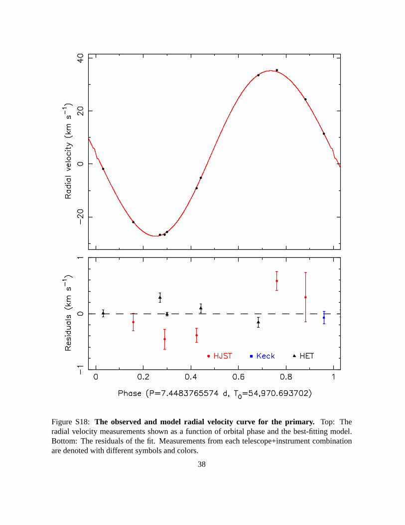
Figure S18: The observed and model radial velocity curve for the primary. Top: Theradial velocity measurements shown as a function of orbitalphase and the best-fitting model.Bottom: The residuals of the fit. Measurements from each telescope+instrument combinationare denoted with different symbols and colors.

38

Kepler−47

To

Ear

th

A

B

b

c

0.5 AU

AB

b

c

Figure S19:Schematic diagrams of the Kepler-47 orbits.Top: A face-on view of the stellarand planetary orbits found from the best-fitting model of theKepler-47 system. The center ofmass of the system is marked with the cross. The stars and the planets would not be seen atthis scale, and so their positions are marked with boxes. Bottom: The view of the system asseen from Earth on an expanded scale is shown. The lines denote the projected orbits of thevarious bodies. Both planets can transit the primary star (labeled A). Transits of the secondarystar (labeled b) are narrowly missed for the best-fitting orbital configuration.

39

Figure S20:Two-parameter joint posterior distributions of primary mo del parameters.The densities are plotted logarithmically in order to elucidate the nature of the parameter cor-relations. The indices listed along the diagonal indicate which parameter is associated withthe corresponding row and column. The parameter name corresponding to a given index isindicated in Table S5 in the first column.

40

0.00 0.02 0.04 0.06 0.08Planet b Eccentricity, eb

0

20

40

60

80

Pro

babi

lity

Den

sity

0.0 0.1 0.2 0.3 0.4 0.5 0.6Planet c Eccentricity, ec

0

2

4

6

8

Pro

babi

lity

Den

sity

Figure S21:Posterior distributions in eccentricity.

41

0.00 0.02 0.04 0.06 0.08Planet b Eccentricity, eb

0

100

200

300P

lane

t b A

rgum

ent o

f Per

iast

ron,

ωb

(deg

)

0.0 0.1 0.2 0.3 0.4 0.5 0.6Planet c Eccentricity, ec

0

100

200

300

Pla

net c

Arg

umen

t of P

eria

stro

n, ω

b (d

eg)

Figure S22:Posterior distributions in the eccentricity and argument of pericenter planes.

42

0.0 0.5 1.0 1.5 2.0 2.5 3.0Orbital Inclination to the Invariable Plane (deg)

0.0

0.5

1.0

1.5

2.0

2.5

Pro

babi

lity

Den

sity

Planet bPlanet c

Figure S23:Posterior distributions in the inclination of the planetary orbits relative to theinvariable plane.

43

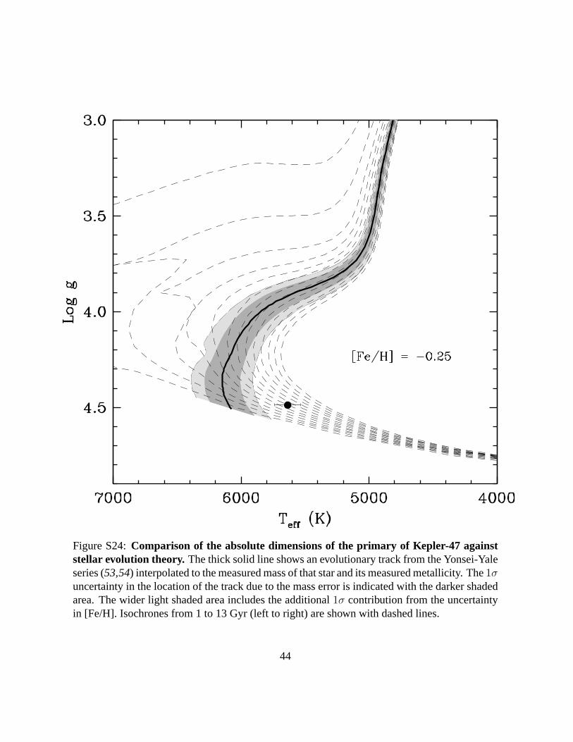
Figure S24:Comparison of the absolute dimensions of the primary of Kepler-47 againststellar evolution theory. The thick solid line shows an evolutionary track from the Yonsei-Yaleseries (53,54) interpolated to the measured mass of that star and its measured metallicity. The1σuncertainty in the location of the track due to the mass erroris indicated with the darker shadedarea. The wider light shaded area includes the additional1σ contribution from the uncertaintyin [Fe/H]. Isochrones from 1 to 13 Gyr (left to right) are shown with dashed lines.

44

Figure S25:Isochrones in the mass-radius and mass-temperature planes. Isochrones fromthe Dartmouth models (56) corresponding to ages from 1 to 13 Gyr, compared against themeasured masses, radii, and temperatures of the stars in Kepler-47. The oldest isochrone isindicated with a solid line, and the metallicity has been setto the spectroscopically determinedvalue of [Fe/H]= −0.25. The error bars for the measurements are represented with the shadedboxes. Top: The mass-radius diagram. The inset shows an enlargement around the secondary,which appears to agree with the models. Bottom: The mass-temperature diagram, showing thesecondary to be cooler than predicted.

45

Table S1:Radial velocities for Kepler-47.

Date UT Time BJD RVA telescopeYYYY-MM-DD (2,455,000+) km s−1

2012-04-10 13:25:48.68 1028.05942 11.442± 0.011 Keck2012-04-23 09:11:27.36 1040.90325 33.534± 0.091 HET2012-05-01 09:52:55.08 1048.93237 35.458± 0.171 HJST2012-05-02 07:23:45.95 1049.82882 24.430± 0.440 HJST2012-05-04 08:34:10.40 1051.88474−21.957± 0.159 HJST2012-05-05 08:08:26.83 1052.86692−26.719± 0.178 HJST2012-05-06 08:08:55.42 1053.86729 −9.150± 0.122 HJST2012-05-18 07:35:21.15 1065.83749 −1.843± 0.060 HET2012-05-20 07:37:07.78 1067.83880−25.681± 0.030 HET2012-06-05 06:29:24.15 1083.79236 −5.223± 0.080 HET2012-06-26 08:03:52.39 1104.85862−26.743± 0.086 HJST

Table S2:Spectroscopic parameters from SPC.

parameter valueTeff (K) 5636± 100

log g (cgs dex) 4.42± 0.10[m/H] (dex) −0.25± 0.08

Vrot sin i (km s−1) 4.1± 0.5

Table S3:Times of stellar eclipses.

cycle # primary corrected uncertainty cycle # secondary uncertaintytime2 time1 (min) time1 (min)

0.0 ... ... ... 0.4873910 -33.12216 2.181.0 -29.30630 -29.30631 0.39 1.4873910 -25.67634 2.582.0 -21.85791 -21.85777 0.37 2.4873910 -18.23125 2.183.0 -14.40955 -14.40931 0.42 3.4873910 -10.78077 2.184.0 -6.96153 -6.96144 0.43 4.4873910 -3.33057 2.185.0 ... ... ... 5.4873910 4.11649 2.186.0 7.93529 7.93560 0.34 6.4873910 11.56631 2.487.0 ... ... ... 7.4873910 19.01194 2.288.0 22.83203 22.83220 0.34 8.4873910 26.46447 2.38

2BJD-2,455,000

46

Table S3: (continued)

9.0 30.28050 30.28080 0.33 9.4873910 33.91396 2.0810.0 37.72889 37.72909 0.32 10.4873910 41.36049 2.2811.0 45.17721 45.17755 0.33 11.4873910 48.80785 2.1812.0 52.62549 52.62570 0.35 12.4873910 ... ...13.0 60.07424 60.07443 0.35 13.4873910 ... ...14.0 67.52268 67.52276 0.44 14.4873910 71.15005 2.1815.0 74.97091 74.97090 0.41 15.4873910 78.60117 2.3816.0 82.41951 82.41949 0.39 16.4873910 86.04829 2.1817.0 89.86795 89.86809 0.39 17.4873910 93.49997 2.1818.0 97.31647 97.31640 0.27 18.4873910 100.94826 2.3819.0 104.76482 104.76476 0.29 19.4873910 108.39407 2.1820.0 112.21316 112.21285 0.37 20.4873910 115.84301 2.1821.0 119.66158 119.66138 0.28 21.4873910 123.29027 2.2822.0 127.10971 127.10951 0.24 22.4873910 130.73599 2.1823.0 134.55816 134.55805 0.38 23.4873910 138.18757 2.2824.0 142.00644 142.00639 0.32 24.4873910 145.63522 2.3825.0 149.45473 149.45475 0.32 25.4873910 153.08287 2.2826.0 ... ... ... 26.4873910 160.53488 2.4827.0 164.35156 164.35158 0.30 27.4873910 167.98079 2.0828.0 171.80006 171.80016 0.34 28.4873910 175.43139 2.1829.0 179.24807 179.24806 0.25 29.4873910 ... ...30.0 186.69626 186.69604 0.33 30.4873910 190.32626 2.1831.0 194.14450 194.14486 0.33 31.4873910 197.77523 2.2832.0 201.59277 201.59307 0.40 32.4873910 205.22572 2.1833.0 209.04129 209.04161 0.48 33.4873910 212.67172 2.1834.0 ... ... ... 34.4873910 220.11933 2.1835.0 223.93826 223.93843 0.41 35.4873910 227.56783 2.2836.0 ... ... ... 36.4873910 235.01738 2.1837.0 238.83553 238.83546 0.31 37.4873910 242.46451 2.1838.0 246.28389 246.28401 0.33 38.4873910 249.91181 2.1839.0 253.73230 253.73247 0.29 39.4873910 257.36186 2.5840.0 261.18019 261.18031 0.25 40.4873910 264.80933 2.1841.0 268.62872 268.62889 0.27 41.4873910 272.25848 2.1842.0 ... ... ... 42.4873910 279.70576 2.1843.0 283.52551 283.52545 0.33 43.4873910 287.15579 2.5844.0 290.97418 290.97397 0.32 44.4873910 294.60501 2.1845.0 298.42259 298.42234 0.38 45.4873910 302.05267 2.1846.0 305.87113 305.87077 0.28 46.4873910 ... ...47.0 313.31965 313.31911 0.33 47.4873910 316.94980 2.18

47

Table S3: (continued)

48.0 320.76803 320.76741 0.31 48.4873910 324.39888 2.1849.0 328.21635 328.21580 0.33 49.4873910 331.84676 2.0850.0 335.66454 335.66432 0.30 50.4873910 339.29309 2.2851.0 343.11269 343.11255 0.27 51.4873910 346.74032 2.1852.0 350.56108 350.56100 0.37 52.4873910 354.18991 2.2853.0 358.00916 358.00920 0.37 53.4873910 361.63907 2.1854.0 365.45750 365.45727 0.35 54.4873910 369.08855 2.1855.0 372.90583 372.90553 0.37 55.4873910 376.53673 2.3856.0 380.35414 380.35434 0.34 56.4873910 383.98453 2.3857.0 387.80274 387.80304 0.29 57.4873910 391.43301 2.3858.0 395.25105 395.25158 0.28 58.4873910 398.88193 2.2859.0 402.69932 402.69981 0.39 59.4873910 406.33048 2.2860.0 410.14753 410.14797 0.39 60.4873910 413.77876 2.4861.0 417.59598 417.59649 0.37 61.4873910 421.22705 2.2862.0 425.04448 425.04486 0.41 62.4873910 428.67664 2.1863.0 432.49299 432.49335 0.39 63.4873910 436.12677 2.4864.0 439.94160 439.94159 0.38 64.4873910 443.57389 2.2865.0 447.38994 447.38962 0.41 65.4873910 451.01777 2.2866.0 454.83858 454.83824 0.42 66.4873910 458.46973 2.2867.0 ... ... ... 67.4873910 465.91872 2.1868.0 469.73590 469.73511 0.49 68.4873910 473.36673 2.1869.0 477.18426 477.18334 0.43 69.4873910 480.80983 2.1870.0 484.63273 484.63184 0.42 70.4873910 488.26371 2.1871.0 492.08030 492.07982 0.29 71.4873910 495.71273 2.0872.0 499.52841 499.52831 0.35 72.4873910 503.15841 2.2873.0 506.97666 506.97688 0.37 73.4873910 510.60646 2.2874.0 514.42490 514.42526 0.33 74.4873910 518.05528 2.1875.0 521.87334 521.87356 0.31 75.4873910 525.50508 2.2876.0 529.32182 529.32216 0.28 76.4873910 532.95444 2.3877.0 536.77016 536.77052 0.27 77.4873910 540.40058 2.2878.0 ... ... ... 78.4873910 547.84725 2.3879.0 551.66689 551.66678 0.32 79.4873910 ... ...80.0 ... ... ... 80.4873910 ... ...81.0 ... ... ... 81.4873910 570.19645 2.8882.0 574.01232 574.01196 0.31 82.4873910 577.64083 2.3883.0 581.46071 581.46061 0.32 83.4873910 585.09178 2.3884.0 588.90872 588.90902 0.35 84.4873910 592.54015 2.1885.0 ... ... ... 85.4873910 599.98822 2.0886.0 603.80549 603.80542 0.56 86.4873910 607.43557 2.28

48

Table S3: (continued)

87.0 611.25410 611.25400 0.53 87.4873910 614.88572 2.0888.0 618.70257 618.70241 0.48 88.4873910 622.33113 2.3889.0 626.15074 626.15090 0.54 89.4873910 629.78026 2.1890.0 633.59939 633.59952 0.47 90.4873910 ... ...91.0 ... ... ... 91.4873910 644.67803 2.1892.0 648.49623 648.49598 0.27 92.4873910 652.12533 2.1893.0 655.94458 655.94414 0.37 93.4873910 659.57425 2.1894.0 663.39318 663.39264 0.31 94.4873910 667.02407 1.9895.0 670.84174 670.84143 0.39 95.4873910 674.47038 2.1896.0 ... ... ... 96.4873910 681.92000 2.2897.0 685.73807 685.73795 0.32 97.4873910 689.37003 2.2898.0 693.18629 693.18620 0.29 98.4873910 696.81581 2.0899.0 700.63456 700.63458 0.28 99.4873910 704.26500 2.08

100.0 708.08304 708.08305 0.29 100.4873910 711.71361 2.08101.0 715.53118 715.53130 0.28 101.4873910 719.16004 2.18102.0 722.97934 722.97955 0.29 102.4873910 726.60875 2.18103.0 730.42778 730.42805 0.22 103.4873910 734.05809 2.18104.0 737.87627 737.87620 0.27 104.4873910 741.50754 2.18105.0 745.32473 745.32472 0.32 105.4873910 748.95596 2.18106.0 752.77319 752.77311 0.27 106.4873910 756.40446 2.28107.0 760.22158 760.22162 0.30 107.4873910 763.85116 2.28108.0 767.66986 767.66997 0.32 108.4873910 771.30069 2.28109.0 775.11818 775.11824 0.33 109.4873910 778.74507 2.28110.0 782.56642 782.56650 0.47 110.4873910 786.19837 2.48111.0 790.01518 790.01521 0.35 111.4873910 793.64804 2.08112.0 797.46374 797.46387 0.37 112.4873910 801.09020 2.28113.0 804.91244 804.91231 0.48 113.4873910 808.54202 2.18114.0 812.36063 812.36030 0.29 114.4873910 815.99029 2.38115.0 819.80879 819.80861 0.20 115.4873910 823.43924 2.18116.0 827.25723 827.25718 0.29 116.4873910 830.88663 2.28117.0 834.70543 834.70552 0.31 117.4873910 838.33915 2.18118.0 842.15352 842.15380 0.32 118.4873910 845.78408 2.18119.0 849.60183 849.60199 0.27 119.4873910 853.23131 2.08120.0 857.05060 857.05057 0.35 120.4873910 860.68308 2.18121.0 864.49914 864.49900 0.30 121.4873910 868.13074 2.08122.0 871.94730 871.94713 0.25 122.4873910 875.57538 2.18123.0 879.39555 879.39559 0.26 123.4873910 883.02764 2.18124.0 886.84395 886.84387 0.27 124.4873910 890.47404 2.08125.0 894.29242 894.29236 0.25 125.4873910 897.92584 2.08

49

Table S3: (continued)

126.0 901.74076 901.74070 0.31 126.4873910 ... ...127.0 909.18926 909.18937 0.27 127.4873910 912.82074 2.28128.0 916.63756 916.63783 0.35 128.4873910 920.26855 2.18129.0 924.08561 924.08598 0.33 129.4873910 927.71411 2.18130.0 ... ... ... 130.4873910 935.16675 2.18131.0 938.98133 938.98223 0.33 131.4873910 942.61285 2.18132.0 946.42970 946.43047 0.33 132.4873910 ... ...133.0 953.87853 953.87896 0.30 133.4873910 957.50762 2.28134.0 961.32731 961.32765 0.31 134.4873910 964.95949 2.68135.0 968.77609 968.77621 0.33 135.4873910 972.40639 2.18136.0 976.22531 976.22515 0.33 136.4873910 979.85442 2.28137.0 983.67397 983.67372 0.34 137.4873910 ... ...138.0 991.12232 991.12194 0.31 138.4873910 ... ...139.0 998.57040 998.56992 0.33 139.4873910 1002.20122 1.98140.0 1006.01835 1006.01771 0.27 140.4873910 ... ...141.0 1013.46672 1013.46612 0.33 141.4873910 ... ...

50

Table S4:Times of planetary transits.

cycle # measured uncertainty duration model model duration notetime3 (minute) (hour) time2 (hour)

Planet b1.0 -30.79061 11.98 4.80 -30.81466 4.502.0 ... ... ... 16.27142 3.81 data gap3.0 65.24000 30.00 6.72 65.24426 6.234.0 112.53000 30.00 3.60 112.54562 3.535.0 160.94000 90.00 11.00 160.90698 10.296.0 208.84245 5.30 3.60 208.84102 3.507.0 256.35001 60.00 8.16 256.32285 7.808.0 305.13831 0.70 3.84 305.12396 3.719.0 352.26001 30.00 5.28 352.25223 5.00

10.0 401.35165 8.06 4.56 401.35574 4.2411.0 448.43933 19.12 4.08 448.42355 3.9412.0 497.42072 60.00 5.76 497.46506 5.5013.0 544.74023 10.37 3.60 544.68713 3.4814.0 593.25055 2.30 9.12 593.26556 8.7715.0 ... ... ... 640.98407 3.29 data gap16.0 688.61578 26.96 9.36 688.65100 8.6517.0 737.27374 10.37 3.60 737.27942 3.3118.0 784.40002 30.00 5.52 784.47644 5.1319.0 ... ... ... 833.53937 3.58 data gap20.0 880.63666 12.21 3.84 880.61505 3.7321.0 ... ... ... 929.71033 4.30 corrupted data22.0 976.86499 60.00 4.08 976.87207 3.06

Planet c1.0 246.64867 5.07 5.76 246.64379 4.022.0 550.47591 5.23 8.16 550.47833 6.123.0 850.99483 5.30 6.96 850.99053 6.00

Orphan1.0 977.363 5.76 4.15 ... ...

3BJD-2,455,000

51

Table S5:Model fitting parameters for the photometric-dynamical model. See the text fordefinitions of the terms. The numbers in boldface refer to theparameters shown in Fig. S20.

Parameter Name Best-fit 50% 15.8% 84.2%Mass parameters

0. Mass of Star A,MA (M⊙) 1.043 1.049 −0.055 +0.0541. Mass ratio, Star B,MB/MA 0.3473 0.3462 −0.0063 +0.0069

Planet b Orbit(Epoch BJD 2,454,969.216)2. Orbital Period,Pb (day) 49.514 49.532 −0.027 +0.0403. Eccentricity Parameter,

√eb cos(ωb) −0.094 0.000 −0.075 +0.067

4. Eccentricity Parameter,√eb sin(ωb) 0.003 0.098 −0.067 +0.042

5. Time of Barycentric Transit,tb (BJD - 2,455,000) −31.367 −31.353 −0.010 +0.011

6. Orbital Inclination,ib (deg) 89.59 89.70 −0.16 +0.507. Relative Nodal Longitude,∆Ωb (deg) 0.10 0.23 −0.21 +0.58

Planet c Orbit(Epoch BJD - 2,455,246.6545)8. Orbital Period,Pc (day) 303.158 303.137 −0.020 +0.0729. Eccentricity Parameter,

√ec cos(ωc) −0.35 −0.04 −0.40 +0.41

10. Eccentricity Parameter,√ec sin(ωc) −0.237 −0.257 −0.041 +0.039

11. Time of Barycentric Transit,tc (BJD - 2,455,000) 246.985 246.997 −0.012 +0.016

12. Orbital Inclination,ic (deg) 89.826 89.825 −0.010 +0.00913. Relative Nodal Longitude,∆Ωc (deg) 1.06 0.99 −0.50 +0.49

Stellar Orbit14. Orbital Period,PAB (day) 7.44837695 7.44837703 −0.00000021 +0.0000002115. Eccentricity Parameter,eEB cos(ωEB) −0.019778 −0.019797 −0.000045 +0.00004416. Eccentricity Parameter,eEB sin(ωEB) −0.0125 −0.0112 −0.0019 +0.001917. Time of Primary Eclipse,

tEB (BJD - 2455000) −29.306346 −29.306342 −0.000018 +0.00001818. Orbital Inclination,iEB (deg) 89.34 89.40 −0.10 +0.12

Radius/Light Parameters19. Linear Limb Darkening Parameter for

Star A,u 0.4151 0.4137 −0.0044 +0.004420. Stellar Flux Ratio,FB/FA (×100) 0.568 0.579 −0.017 +0.01721. Density of Star A,ρA (g cm−3) 1.163 1.176 −0.025 +0.02422. Radius Ratio, Star B,RB/RA 0.3636 0.3671 −0.0047 +0.004723. Planetary Radius Ratio,Rb/RA 0.0283 0.0289 −0.0011 +0.001124. Planetary Radius Ratio,Rc/RA 0.0439 0.0440 −0.0018 +0.0017

Relative Contamination,100× (Fcont/FA)

Season 0 −2.9 −0.9 −2.8 +2.8Season 1 −1.5 0.5 −2.8 +2.9Season 2 −2.8 −0.8 −2.8 +2.8Season 3 −1.9 0.1 −2.8 +2.9

Noise ParameterLong Cadence Relative Width,σLC (×105) 62.95 62.75 −0.42 +0.43

Radial Velocity ParametersRV Offset,γ (km s−1) 4.67 4.60 −0.23 +0.22Zero-level Diff.,∆γ (km s−1) −0.12 −0.01 −0.31 +0.30RV Jitter,σRV (km s−1) 0.31 0.43 −0.12 +0.19

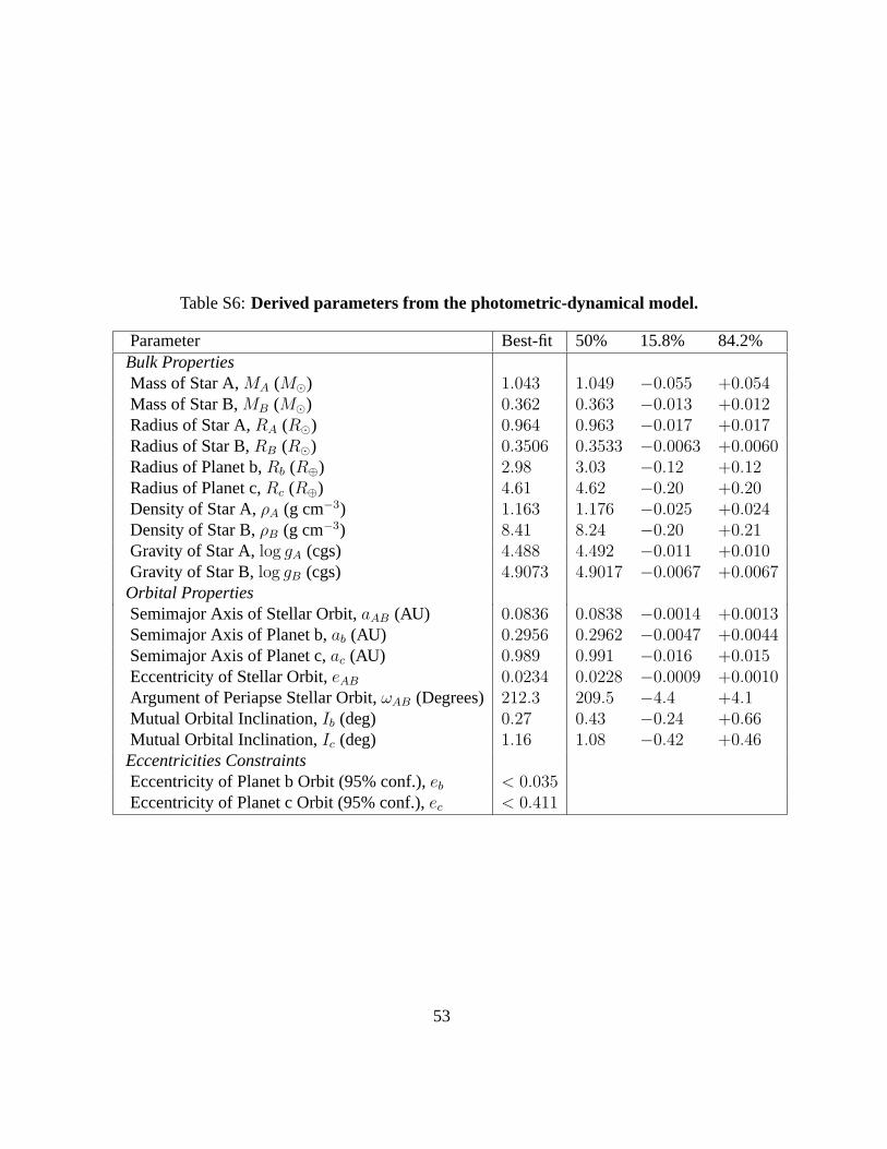
Table S6:Derived parameters from the photometric-dynamical model.

Parameter Best-fit 50% 15.8% 84.2%Bulk PropertiesMass of Star A,MA (M⊙) 1.043 1.049 −0.055 +0.054Mass of Star B,MB (M⊙) 0.362 0.363 −0.013 +0.012Radius of Star A,RA (R⊙) 0.964 0.963 −0.017 +0.017Radius of Star B,RB (R⊙) 0.3506 0.3533 −0.0063 +0.0060Radius of Planet b,Rb (R⊕) 2.98 3.03 −0.12 +0.12Radius of Planet c,Rc (R⊕) 4.61 4.62 −0.20 +0.20Density of Star A,ρA (g cm−3) 1.163 1.176 −0.025 +0.024Density of Star B,ρB (g cm−3) 8.41 8.24 −0.20 +0.21Gravity of Star A,log gA (cgs) 4.488 4.492 −0.011 +0.010Gravity of Star B,log gB (cgs) 4.9073 4.9017 −0.0067 +0.0067Orbital PropertiesSemimajor Axis of Stellar Orbit,aAB (AU) 0.0836 0.0838 −0.0014 +0.0013Semimajor Axis of Planet b,ab (AU) 0.2956 0.2962 −0.0047 +0.0044Semimajor Axis of Planet c,ac (AU) 0.989 0.991 −0.016 +0.015Eccentricity of Stellar Orbit,eAB 0.0234 0.0228 −0.0009 +0.0010Argument of Periapse Stellar Orbit,ωAB (Degrees) 212.3 209.5 −4.4 +4.1Mutual Orbital Inclination,Ib (deg) 0.27 0.43 −0.24 +0.66Mutual Orbital Inclination,Ic (deg) 1.16 1.08 −0.42 +0.46Eccentricities ConstraintsEccentricity of Planet b Orbit (95% conf.),eb < 0.035Eccentricity of Planet c Orbit (95% conf.),ec < 0.411

53

Table S7:Predicted transit times for planet b.

Epoch T0-2,455,000 BJD Impact Parameter Transit Velocity (RA/day) Duration (hr)22 1025.630± 0.035 0.527± 0.237 6.007± 0.094 7.069± 0.96323 1073.156± 0.022 0.602± 0.265 12.496± 0.136 3.209± 0.60524 1121.106± 0.075 0.528± 0.236 4.522± 0.086 9.353± 1.33925 1169.457± 0.033 0.642± 0.261 12.282± 0.111 3.170± 0.68126 1216.768± 0.072 0.577± 0.246 7.221± 0.260 5.674± 0.96027 1265.733± 0.050 0.691± 0.261 11.318± 0.129 3.280± 0.80928 1312.836± 0.073 0.654± 0.255 9.880± 0.268 3.885± 0.84729 1361.940± 0.081 0.742± 0.266 9.580± 0.264 3.667± 1.04130 1409.062± 0.083 0.745± 0.269 11.584± 0.213 3.016± 0.85231 1457.985± 0.149 0.774± 0.275 7.030± 0.490 4.897± 1.51432 1505.349± 0.099 0.838± 0.288 12.403± 0.124 2.596± 0.84033 1553.638± 0.299 0.783± 0.285 4.552± 0.261 7.406± 2.19734 1601.654± 0.123 0.917± 0.312 12.433± 0.137 2.454± 0.87235 1649.136± 0.281 0.835± 0.301 6.085± 0.750 5.389± 1.84536 1697.947± 0.159 0.963± 0.342 11.752± 0.363 2.532± 0.94937 1745.100± 0.235 0.917± 0.331 9.008± 0.752 3.496± 1.23538 1794.188± 0.221 0.994± 0.374 10.313± 0.726 2.827± 1.07639 1841.284± 0.229 0.993± 0.368 11.053± 0.532 2.678± 1.01840 1890.314± 0.359 1.000± 0.403 8.063± 1.181 3.692± 1.56041 1937.556± 0.243 1.053± 0.409 12.181± 0.256 2.402± 0.90442 1986.153± 0.619 0.989± 0.425 5.333± 0.940 5.488± 2.23043 2033.860± 0.275 1.090± 0.447 12.458± 0.233 2.257± 0.89744 2081.589± 0.657 1.009± 0.445 5.096± 1.232 5.669± 2.27345 2130.158± 0.328 1.106± 0.478 12.073± 0.675 2.389± 0.95646 2177.380± 0.519 1.058± 0.472 7.999± 1.540 3.815± 1.70147 2226.418± 0.429 1.093± 0.498 10.920± 1.298 2.676± 1.11748 2273.503± 0.452 1.095± 0.498 10.406± 1.157 2.930± 1.21149 2322.594± 0.652 1.059± 0.509 8.952± 1.842 3.420± 1.70850 2369.745± 0.442 1.110± 0.516 11.826± 0.654 2.554± 1.03951 2418.551± 0.948 1.027± 0.513 6.479± 1.596 4.824± 2.19052 2466.039± 0.467 1.100± 0.522 12.314± 0.439 2.437± 0.94253 2514.061± 1.048 1.007± 0.515 5.318± 1.565 5.741± 2.27754 2562.341± 0.533 1.066± 0.516 12.245± 1.000 2.523± 0.98055 2609.673± 0.888 1.007± 0.514 7.041± 2.193 4.574± 2.17656 2658.612± 0.680 1.006± 0.499 11.336± 1.781 2.798± 1.20457 2705.720± 0.731 1.003± 0.504 9.729± 1.868 3.343± 1.55658 2754.815± 0.941 0.933± 0.477 9.607± 2.221 3.583± 1.85859 2801.933± 0.665 0.977± 0.482 11.443± 1.205 2.886± 1.109

54

Table S7: (continued)

60 2850.864± 1.217 0.872± 0.453 7.453± 2.025 4.872± 2.18261 2898.207± 0.665 0.931± 0.450 12.091± 0.809 2.810± 0.89762 2946.504± 1.336 0.826± 0.428 6.071± 1.878 5.869± 2.22363 2994.499± 0.731 0.874± 0.411 12.231± 1.283 2.896± 0.92264 3041.964± 1.214 0.796± 0.400 6.417± 2.481 5.578± 2.38565 3090.777± 0.898 0.799± 0.370 11.615± 1.982 3.255± 1.36766 3137.912± 0.997 0.778± 0.366 9.062± 2.402 4.034± 1.86667 3187.001± 1.142 0.713± 0.332 10.124± 2.354 3.862± 1.93168 3234.085± 0.863 0.728± 0.329 11.034± 1.705 3.445± 1.23469 3283.097± 1.385 0.623± 0.298 8.157± 2.238 4.894± 2.19970 3330.344± 0.823 0.663± 0.292 11.893± 1.143 3.340± 0.83271 3378.853± 1.505 0.548± 0.267 6.752± 2.073 6.129± 2.17972 3426.633± 0.871 0.579± 0.265 12.139± 1.403 3.476± 1.016

55

Table S8:Predicted transit times for planet c.

Epoch T0-2,455,000 BJD Impact Parameter Transit Velocity (RA/day) Duration (hr)3 1154.756± 0.011 0.430± 0.056 8.131± 0.133 4.735± 0.2604 1458.197± 0.264 0.397± 1.258 3.369± 0.217 12.967± 1.0005 1758.963± 0.024 0.446± 0.057 7.600± 0.135 5.086± 0.2786 2062.831± 0.033 0.407± 0.114 7.249± 0.145 5.953± 0.4627 2363.464± 0.076 0.458± 0.066 4.141± 0.258 9.823± 0.7838 2667.055± 0.045 0.436± 0.116 8.195± 0.150 5.217± 0.4179 2970.751± 0.085 0.462± 0.164 5.117± 0.316 9.026± 0.981

10 3271.295± 0.083 0.462± 0.118 6.923± 0.195 6.232± 0.48711 3575.153± 0.080 0.461± 0.172 7.787± 0.236 5.922± 0.561

Table S9:ELC model parameters.

Parameter Best fite 0.0306± 0.0071

ω (deg) 226± 12RA/a 0.05322± 0.00068RB/a 0.01935± 0.00029

Teff,B/Teff,A 0.5958± 0.0035i (deg) 89.69± 0.16xA 0.30± 0.13yA 0.38± 0.27

56