Supplementary Information Woody biomass production lags ... · pines (Pinus sylvestris L.) in the...
25
SUPPLEMENTARY INFORMATION DOI: 10.1038/NPLANTS.2015.160 NATURE PLANTS | www.nature.com/natureplants 1 Woody biomass production lags stem-girth increase by over one month in coniferous forests Henri E. Cuny, Cyrille B.K. Rathgeber, David Frank, Patrick Fonti, Harri Mäkinen, Peter Prislan, Sergio Rossi, Edurne Martinez del Castillo, Filipe Campelo, Hanuš Vavrčík, Jesus Julio Camarero, Marina V. Bryukhanova, Tuula Jyske, Jožica Gričar, Vladimír Gryc, Martin De Luis, Joana Vieira, Katarina Čufar, Alexander V. Kirdyanov, Walter Oberhuber, Vaclav Treml, Jian-Guo Huang, Xiaoxia Li, Irene Swidrak, Annie Deslauriers, Eryuan Liang, Pekka Nöjd, Andreas Gruber, Cristina Nabais, Hubert Morin, Cornelia Krause, Gregory King & Meriem Fournier.
Transcript of Supplementary Information Woody biomass production lags ... · pines (Pinus sylvestris L.) in the...
SUPPLEMENTARY INFORMATIONDOI: 10.1038/NPLANTS.2015.160
NATURE PLANTS | www.nature.com/natureplants 1
1
Supplementary Information
Woody biomass production lags stem-girth increase by over one month in coniferous
forests
Henri E. Cuny, Cyrille B.K. Rathgeber, David Frank, Patrick Fonti, Harri Mäkinen, Peter
Prislan, Sergio Rossi, Edurne Martinez del Castillo, Filipe Campelo, Hanuš Vavrčík, Jesus
Julio Camarero, Marina V. Bryukhanova, Tuula Jyske, Jožica Gričar, Vladimír Gryc, Martin
De Luis, Joana Vieira, Katarina Čufar, Alexander V. Kirdyanov, Walter Oberhuber, Vaclav
Treml, Jian-Guo Huang, Xiaoxia Li, Irene Swidrak, Annie Deslauriers, Eryuan Liang, Pekka
Nöjd, Andreas Gruber, Cristina Nabais, Hubert Morin, Cornelia Krause, Gregory King &
Meriem Fournier.
2 NATURE PLANTS | www.nature.com/natureplants
SUPPLEMENTARY INFORMATION DOI: 10.1038/NPLANTS.2015.160
2
Supplementary Methods
Study sites for detailed monitoring of wood formation
Three intensively studied sites were selected in mixed mature temperate forests
composed of silver firs (Abies alba Mill.), Norway spruces (Picea abies [L.] Karst.) and Scots
pines (Pinus sylvestris L.) in the Vosges Mountains (northeast France). The three sites were
spread on a north-south axis of about 15 km and were named according to the closest town:
Walscheid (370 m ASL, 48°38’N, 7°09’E), Abreschviller (430 m ASL, 48°36’N, 7°08’E) and
Grandfontaine (650 m ASL, 48°28’N, 7°08’E). On each site, pits were dug to depict soil
profiles, and complete inventories were built to describe stand structure. Based on these
inventories, five dominant and healthy trees of silvers fir, Norway spruce and Scots pine were
selected on each site, for a total of 45 studied trees (5 trees × 3 species × 3 sites) for 3 years
(2007–2009) of wood formation monitoring (Supplementary Table 2).
Dendrometer and meteorological data
Manual band dendrometers (DB-20, EMS Brno, Czech Republic) were installed at
breast height in March 2007 on the stem of all selected trees, after the removal of most part of
the dead bark, and were read weekly thereafter to monitor stem circumference variations.
Changes in stem girth measured by band dendrometers were transformed into stem radial
variations assuming a circular cross section of the stem.
Daily meteorological data (temperature, precipitation, cumulative global radiation, wind
speed, and relative air humidity) of the monitoring period were gathered from three
meteorological stations, each of them located less than 2 km from the corresponding site.
Modelling soil water balance and characterising the seasonality of environmental factors
3
We used the model Biljou© to assess the daily water balance of the three studied
stands during the three monitoring years (https://appgeodb.nancy.inra.fr/biljou/)1. In addition
to the daily meteorological data mentioned above, the model takes as input soil (e.g., number
and depth of layers, and proportion of fine roots per layer), and stand (forest type and
maximum leaf area index) parameters, and gives as output the relative extractable water
(REW) on a daily scale. The REW is a relative expression of the filling state of the soil: REW
is 100% at field capacity, and 0% at the permanent wilting point. Water stress is assumed to
occur when the REW drops below a threshold of 40%, under which transpiration gradually
decreases due to stomata closure1.
Daily water balance and meteorological data (temperature and light radiation) were
smoothed using generalised additive models (GAMs) in order to obtain representative
seasonal trends of climatic conditions2. GAMs were fitted in R3 using the mgcv package4.
Xylem collection, preparation and observation
To monitor tree-ring formation of each selected tree, small wood samples (2 mm thick
and 1.5 cm long microcores including the phloem, cambial zone, the forming ring and some
previous rings) were collected weekly on tree stem, from April to November during three
years (2007–2009), for a total of about 32 microcores per tree and per year. Microcores were
collected at breast height on the stems of the selected trees using a Trephor® (Vitzani,
Belluno, Italy)5. The injury by a 1.5–2.5 mm diameter corer stimulates growth for about 2 mm
on each side of the wound and for about 1 cm above and below6. Thus, for each tree the
orientation on the stem of the first sampling was randomly selected among the four cardinal
points, and successive microcores were then taken about 1 cm apart from each other and
following a slightly ascending spiral pattern (about 30 cm in height between the first and the
last sample of the year)7 to avoid wound reaction without considerably increasing the
NATURE PLANTS | www.nature.com/natureplants 3
SUPPLEMENTARY INFORMATIONDOI: 10.1038/NPLANTS.2015.160
2
Supplementary Methods
Study sites for detailed monitoring of wood formation
Three intensively studied sites were selected in mixed mature temperate forests
composed of silver firs (Abies alba Mill.), Norway spruces (Picea abies [L.] Karst.) and Scots
pines (Pinus sylvestris L.) in the Vosges Mountains (northeast France). The three sites were
spread on a north-south axis of about 15 km and were named according to the closest town:
Walscheid (370 m ASL, 48°38’N, 7°09’E), Abreschviller (430 m ASL, 48°36’N, 7°08’E) and
Grandfontaine (650 m ASL, 48°28’N, 7°08’E). On each site, pits were dug to depict soil
profiles, and complete inventories were built to describe stand structure. Based on these
inventories, five dominant and healthy trees of silvers fir, Norway spruce and Scots pine were
selected on each site, for a total of 45 studied trees (5 trees × 3 species × 3 sites) for 3 years
(2007–2009) of wood formation monitoring (Supplementary Table 2).
Dendrometer and meteorological data
Manual band dendrometers (DB-20, EMS Brno, Czech Republic) were installed at
breast height in March 2007 on the stem of all selected trees, after the removal of most part of
the dead bark, and were read weekly thereafter to monitor stem circumference variations.
Changes in stem girth measured by band dendrometers were transformed into stem radial
variations assuming a circular cross section of the stem.
Daily meteorological data (temperature, precipitation, cumulative global radiation, wind
speed, and relative air humidity) of the monitoring period were gathered from three
meteorological stations, each of them located less than 2 km from the corresponding site.
Modelling soil water balance and characterising the seasonality of environmental factors
3
We used the model Biljou© to assess the daily water balance of the three studied
stands during the three monitoring years (https://appgeodb.nancy.inra.fr/biljou/)1. In addition
to the daily meteorological data mentioned above, the model takes as input soil (e.g., number
and depth of layers, and proportion of fine roots per layer), and stand (forest type and
maximum leaf area index) parameters, and gives as output the relative extractable water
(REW) on a daily scale. The REW is a relative expression of the filling state of the soil: REW
is 100% at field capacity, and 0% at the permanent wilting point. Water stress is assumed to
occur when the REW drops below a threshold of 40%, under which transpiration gradually
decreases due to stomata closure1.
Daily water balance and meteorological data (temperature and light radiation) were
smoothed using generalised additive models (GAMs) in order to obtain representative
seasonal trends of climatic conditions2. GAMs were fitted in R3 using the mgcv package4.
Xylem collection, preparation and observation
To monitor tree-ring formation of each selected tree, small wood samples (2 mm thick
and 1.5 cm long microcores including the phloem, cambial zone, the forming ring and some
previous rings) were collected weekly on tree stem, from April to November during three
years (2007–2009), for a total of about 32 microcores per tree and per year. Microcores were
collected at breast height on the stems of the selected trees using a Trephor® (Vitzani,
Belluno, Italy)5. The injury by a 1.5–2.5 mm diameter corer stimulates growth for about 2 mm
on each side of the wound and for about 1 cm above and below6. Thus, for each tree the
orientation on the stem of the first sampling was randomly selected among the four cardinal
points, and successive microcores were then taken about 1 cm apart from each other and
following a slightly ascending spiral pattern (about 30 cm in height between the first and the
last sample of the year)7 to avoid wound reaction without considerably increasing the

4 NATURE PLANTS | www.nature.com/natureplants
SUPPLEMENTARY INFORMATION DOI: 10.1038/NPLANTS.2015.160
4
influence of stem circumferential variability on the final dataset.
Microcores were prepared in the laboratory, and transverse sections with 5–10 µm in
thickness were cut with a rotary microtome (HM 355S, MM France). Sections were stained
with cresyl violet acetate and permanently mounted on glass slides using Histolaque LMR®.
Overall, about 4,300 anatomical sections were analysed using an optical microscope
(AxioImager.M2, Carl Zeiss SAS, France) to track tree-ring formation. Sections were
observed under visible and polarised light, at ×100–400 magnification. Resin ducts are
anatomical features normally produced in Scots pine and Norway spruce wood, whereas they
only appear in response to wounding in silver fir. However, for the three species, resin ducts
were scarce on the sections, so that the anatomical observations and cell counting were always
performed on tracheid radial files having no resin ducts.
We distinguished and counted the cambial, enlarging, wall thickening and mature cells
along at least three radial files of the forming tree ring. Cells of the cambial zone divide by
mitosis to produce xylem cells on the pith side, and phloem cells on the bark side. They had
rectangular shape, thin primary walls and small radial diameters, around 5–8 µm. Once
produced, xylem cells enter the enlargement phase, where they undergo marked radial
diameter increase under turgor pressure and deposition of primary wall material8. Therefore,
we described enlarging cells as being at least two times larger than cambial cells, but still
surrounded by thin walls. After enlargement, cells undergo secondary wall formation and
lignification (of both primary and secondary walls). The formation of the multi-layered
secondary wall starts with the deposition of cellulose and hemicellulose microfibrils9, while
lignin is deposited afterwards in the remaining spaces to cement the microfibrils together10.
Because secondary wall formation and lignification processes largely overlap, they were not
discriminated and regrouped under the term “wall thickening”. We distinguished thickening
cells thanks to the birefringence of the secondary walls — cellulose microfibrils are deposited
5
according to a particular orientation in the secondary wall that makes them shining under
polarised light11. Furthermore, cresyl violet acetate staining, whereby cellulose is stained
purple and lignin blue12, was used to follow the advancement of lignification. So, thickening
cells exhibited violet and blue walls, indicating that lignification was in progress, whereas
mature tracheids exhibited plain blue walls, indicating that lignification was over. To reduce
the noise due to eccentric growth in the dataset, current cell counts were standardised by
previous year cell number13, using the R package CAVIAR3,14.
Characterisation of wood formation dynamics
In order to characterise intra-annual wood formation dynamics, we fitted generalised
additive models (GAMs) on the standardised number of cells counted weekly in the cambial,
enlargement, wall thickening, and mature zones of xylem differentiation2. Thanks to their
flexibility, GAMs have proved to be particularly well-suitable to model the complex intra-
annual patterns that characterise wood formation dynamics2, and thus to accurately quantify
the kinetics of xylem cell development15.
GAMs are semi-parametric extensions of GLMs, which are themselves mathematical
extensions of linear models4,16. Let us consider the linear model which has the form:
Y = α + Xβ + ε (1)
where Y denotes the response variable, α is a constant called the intercept, X = (X1, … Xp) is
the matrix of p predictor variables, β = (β1, …, βp) is the vector of p regression coefficients
(one for each predictor), and ε is the error term. Two main assumptions limit the use of this
linear model: (a) the errors are assumed to follow a normal (Gaussian) distribution and to
have a constant variance; (b) the predictors are assumed to have a linear effect on the response
variable. By applying a mathematical transformation to the response variable Y according to
the real distribution of the errors, GLMs relax these assumptions and thus generalise the linear
NATURE PLANTS | www.nature.com/natureplants 5
SUPPLEMENTARY INFORMATIONDOI: 10.1038/NPLANTS.2015.160
4
influence of stem circumferential variability on the final dataset.
Microcores were prepared in the laboratory, and transverse sections with 5–10 µm in
thickness were cut with a rotary microtome (HM 355S, MM France). Sections were stained
with cresyl violet acetate and permanently mounted on glass slides using Histolaque LMR®.
Overall, about 4,300 anatomical sections were analysed using an optical microscope
(AxioImager.M2, Carl Zeiss SAS, France) to track tree-ring formation. Sections were
observed under visible and polarised light, at ×100–400 magnification. Resin ducts are
anatomical features normally produced in Scots pine and Norway spruce wood, whereas they
only appear in response to wounding in silver fir. However, for the three species, resin ducts
were scarce on the sections, so that the anatomical observations and cell counting were always
performed on tracheid radial files having no resin ducts.
We distinguished and counted the cambial, enlarging, wall thickening and mature cells
along at least three radial files of the forming tree ring. Cells of the cambial zone divide by
mitosis to produce xylem cells on the pith side, and phloem cells on the bark side. They had
rectangular shape, thin primary walls and small radial diameters, around 5–8 µm. Once
produced, xylem cells enter the enlargement phase, where they undergo marked radial
diameter increase under turgor pressure and deposition of primary wall material8. Therefore,
we described enlarging cells as being at least two times larger than cambial cells, but still
surrounded by thin walls. After enlargement, cells undergo secondary wall formation and
lignification (of both primary and secondary walls). The formation of the multi-layered
secondary wall starts with the deposition of cellulose and hemicellulose microfibrils9, while
lignin is deposited afterwards in the remaining spaces to cement the microfibrils together10.
Because secondary wall formation and lignification processes largely overlap, they were not
discriminated and regrouped under the term “wall thickening”. We distinguished thickening
cells thanks to the birefringence of the secondary walls — cellulose microfibrils are deposited
5
according to a particular orientation in the secondary wall that makes them shining under
polarised light11. Furthermore, cresyl violet acetate staining, whereby cellulose is stained
purple and lignin blue12, was used to follow the advancement of lignification. So, thickening
cells exhibited violet and blue walls, indicating that lignification was in progress, whereas
mature tracheids exhibited plain blue walls, indicating that lignification was over. To reduce
the noise due to eccentric growth in the dataset, current cell counts were standardised by
previous year cell number13, using the R package CAVIAR3,14.
Characterisation of wood formation dynamics
In order to characterise intra-annual wood formation dynamics, we fitted generalised
additive models (GAMs) on the standardised number of cells counted weekly in the cambial,
enlargement, wall thickening, and mature zones of xylem differentiation2. Thanks to their
flexibility, GAMs have proved to be particularly well-suitable to model the complex intra-
annual patterns that characterise wood formation dynamics2, and thus to accurately quantify
the kinetics of xylem cell development15.
GAMs are semi-parametric extensions of GLMs, which are themselves mathematical
extensions of linear models4,16. Let us consider the linear model which has the form:
Y = α + Xβ + ε (1)
where Y denotes the response variable, α is a constant called the intercept, X = (X1, … Xp) is
the matrix of p predictor variables, β = (β1, …, βp) is the vector of p regression coefficients
(one for each predictor), and ε is the error term. Two main assumptions limit the use of this
linear model: (a) the errors are assumed to follow a normal (Gaussian) distribution and to
have a constant variance; (b) the predictors are assumed to have a linear effect on the response
variable. By applying a mathematical transformation to the response variable Y according to
the real distribution of the errors, GLMs relax these assumptions and thus generalise the linear
6 NATURE PLANTS | www.nature.com/natureplants
SUPPLEMENTARY INFORMATION DOI: 10.1038/NPLANTS.2015.160
6
model to non-linear responses (but the linearity of components contributing to the predictor is
preserved) and variables that can have other than a normal distribution (hence the name
Generalised Linear Models), including the normal, binomial, Poisson, or gamma probability
distributions17,18. The mathematical function used to transform the response variable is called
the “link function” because it provides the relationship between the linear predictor (Xβ) and
the expected value of the response variable Y, so that a GLM takes the form:
g(E(Y)) = α + Xβ + ε (2)
where g() is the link function, E(Y) is the expected value of Y and α, X, and β are those
previously described in Eq. (1). The link function depends on the distribution of the response
variable (and so of its error). In this study, the response variable corresponds to the number of
cells weekly counted in the wood formation phases. Count data followed a Poisson
distribution, and in this case the link function used is the log function (the model is a log-
linear model). Note that if the variable follows a normal distribution with a constant variance,
the link function is the identity function g(E(Y))) = Y, so that we obtained the classical linear
model we saw in Eq. (1), which can be considered as a special case of GLMs.
A GAM is a GLM in which the linear predictor depends, in part, on a sum of smooth
functions of predictors4. As for GLMs, the probability distribution of the response variable
must still be specified. Therefore, GAMs are a semi-parametric generalisation of GLMs, and
they take the form:
𝑔𝑔(𝐸𝐸(𝑌𝑌)) = 𝛼𝛼 + 𝑋𝑋𝑋𝑋 + ∑𝑠𝑠𝑗𝑗(𝑋𝑋𝑗𝑗) + 𝜀𝜀 (3)
where X = (X1, …, Xp) is a matrix for any strictly parametric model components with
parameter vector β, sj() are unspecified smooth functions for the covariates Xj, and g(), E(Y)
and α are those previously described in Eq. (1) and (2).
The strength of GAMs lies in their flexibility, i.e. their ability to deal with non-linear
and non-monotonic relationships between the response and the set of explanatory variables.
7
This is because the data determine the nature of the relationship between the response and the
set of explanatory variables rather than assuming some form of parametric relationship16,19.
GAMs are thus referred to as being data driven rather than model driven, because the data
determine the nature of the relationship between the response variable and the set of
explanatory variables rather than assuming a certain type of parametric relationship16.
Because of their flexibility, GAMs have proved to be particularly well-suitable to model the
complex intra-annual patterns that characterise wood formation dynamics2, and thus to
accurately quantify the kinetics of xylem cell development15.
In the case of wood formation dynamics, we want to express the response variables,
corresponding to the number of cells weekly counted in the wood formation phases, as a
function of the day of year. Thus, the expression of our GAM simply began:
𝑙𝑙𝑙𝑙𝑙𝑙(𝐸𝐸(𝑁𝑁)) = 𝛼𝛼 + 𝑠𝑠(𝐷𝐷𝐷𝐷) + 𝜀𝜀 (4)
where N is the vector of the number of cells weekly counted in the considered phase, and DY
is the vector of the corresponding days of year.
GAMs were fitted in R3 using the mgcv package4 for every year on each individual tree.
The values of the fitted models were then averaged to calculate means representing the
general wood formation dynamics by species, site, and year.
For each mean series, the daily rate of xylem cell production was calculated as the
difference between the total numbers of cells predicted by GAMs on the consecutive days.
Moreover, we used the average cell numbers predicted by GAMs to calculate the date of
entrance of each cell in each development zone (cambial, enlargement, wall thickening and
mature zones)2. From these dates, the durations spent by each cell in the enlargement and wall
thickening zone were computed. The rates of radial diameter enlargement and wall deposition
were computed for each cell by dividing its final dimensions (cell radial diameter and wall
NATURE PLANTS | www.nature.com/natureplants 7
SUPPLEMENTARY INFORMATIONDOI: 10.1038/NPLANTS.2015.160
6
model to non-linear responses (but the linearity of components contributing to the predictor is
preserved) and variables that can have other than a normal distribution (hence the name
Generalised Linear Models), including the normal, binomial, Poisson, or gamma probability
distributions17,18. The mathematical function used to transform the response variable is called
the “link function” because it provides the relationship between the linear predictor (Xβ) and
the expected value of the response variable Y, so that a GLM takes the form:
g(E(Y)) = α + Xβ + ε (2)
where g() is the link function, E(Y) is the expected value of Y and α, X, and β are those
previously described in Eq. (1). The link function depends on the distribution of the response
variable (and so of its error). In this study, the response variable corresponds to the number of
cells weekly counted in the wood formation phases. Count data followed a Poisson
distribution, and in this case the link function used is the log function (the model is a log-
linear model). Note that if the variable follows a normal distribution with a constant variance,
the link function is the identity function g(E(Y))) = Y, so that we obtained the classical linear
model we saw in Eq. (1), which can be considered as a special case of GLMs.
A GAM is a GLM in which the linear predictor depends, in part, on a sum of smooth
functions of predictors4. As for GLMs, the probability distribution of the response variable
must still be specified. Therefore, GAMs are a semi-parametric generalisation of GLMs, and
they take the form:
𝑔𝑔(𝐸𝐸(𝑌𝑌)) = 𝛼𝛼 + 𝑋𝑋𝑋𝑋 + ∑𝑠𝑠𝑗𝑗(𝑋𝑋𝑗𝑗) + 𝜀𝜀 (3)
where X = (X1, …, Xp) is a matrix for any strictly parametric model components with
parameter vector β, sj() are unspecified smooth functions for the covariates Xj, and g(), E(Y)
and α are those previously described in Eq. (1) and (2).
The strength of GAMs lies in their flexibility, i.e. their ability to deal with non-linear
and non-monotonic relationships between the response and the set of explanatory variables.
7
This is because the data determine the nature of the relationship between the response and the
set of explanatory variables rather than assuming some form of parametric relationship16,19.
GAMs are thus referred to as being data driven rather than model driven, because the data
determine the nature of the relationship between the response variable and the set of
explanatory variables rather than assuming a certain type of parametric relationship16.
Because of their flexibility, GAMs have proved to be particularly well-suitable to model the
complex intra-annual patterns that characterise wood formation dynamics2, and thus to
accurately quantify the kinetics of xylem cell development15.
In the case of wood formation dynamics, we want to express the response variables,
corresponding to the number of cells weekly counted in the wood formation phases, as a
function of the day of year. Thus, the expression of our GAM simply began:
𝑙𝑙𝑙𝑙𝑙𝑙(𝐸𝐸(𝑁𝑁)) = 𝛼𝛼 + 𝑠𝑠(𝐷𝐷𝐷𝐷) + 𝜀𝜀 (4)
where N is the vector of the number of cells weekly counted in the considered phase, and DY
is the vector of the corresponding days of year.
GAMs were fitted in R3 using the mgcv package4 for every year on each individual tree.
The values of the fitted models were then averaged to calculate means representing the
general wood formation dynamics by species, site, and year.
For each mean series, the daily rate of xylem cell production was calculated as the
difference between the total numbers of cells predicted by GAMs on the consecutive days.
Moreover, we used the average cell numbers predicted by GAMs to calculate the date of
entrance of each cell in each development zone (cambial, enlargement, wall thickening and
mature zones)2. From these dates, the durations spent by each cell in the enlargement and wall
thickening zone were computed. The rates of radial diameter enlargement and wall deposition
were computed for each cell by dividing its final dimensions (cell radial diameter and wall
8 NATURE PLANTS | www.nature.com/natureplants
SUPPLEMENTARY INFORMATION DOI: 10.1038/NPLANTS.2015.160
8
cross area) – measured from image analysis of the entirely formed tree ring at the end of the
season15 – by the duration spent in the corresponding phase.
Calculation of the rate of stem radial variations
To assess the dynamics of stem radial variations, GAMs were fitted on stem radial size
measurements for every year, every site, and each individual tree of each species. Fittings
were then pooled together to represent the general dynamics of stem radial size variations by
species, site, and year. The daily rate of stem radial variation was calculated as the daily
differences in the stem radial variations predicted using GAMs.
Calculation of the daily rate of xylem size increase
The daily rate of xylem size increase was calculated from the rate of xylem cell
production through cambial cell division, the radial diameter of the cambial cells, and the
individual rates of cell diameter enlargement in the enlargement zone (Supplementary Fig. 1).
First, we measured the radial diameter of cambial cells during the growing season using the
measurement software VideometTM (Microvision instruments, France). We found values close
to 7 µm for the different species, year, and sites (Supplementary Table 3). Therefore, we
assumed that each cambial division leads to the formation of new cells of 7 µm in diameter.
So, the daily rate of xylem size increase provided by the cambial zone (XSICZ, µm day-1) is
calculated simply by multiplying the rate of xylem cell production (rC, cell day-1) by 7 µm
cell-1.
Moreover, the daily rate of xylem size increase provided by the enlargement zone
(XSIEZ, µm day-1) was calculated as the sum of the individual rates of cell enlargement:
XSIEZ =∑ rE,inE
i=1
9
where nE is the daily number of cells in the enlargement zone, and rE,i is the enlargement rate
(µm day-1) of the cell i of the nE cells.
The daily xylem size increase (XSI) was finally calculated as the sum of the contributions of
xylem cell production and enlargement:
XSI = XSICZ + XSIEZ
Calculation of the daily rate of woody biomass production
The rates of xylem cell production and cellular differentiation were used to calculate
the daily rate woody biomass production (Supplementary Fig. 1). First, a rate of primary wall
deposition in the cambial zone was calculated from the rate of xylem cell production (rC)
through cambial cell division in the cambium and the thickness of the primary cell walls. For
that, we measured the primary wall thickness during the growing season using VideometTM
(Microvision instruments, France) and found values close to 0.5 µm for the different species,
year, and sites (Supplementary Table 3). Therefore, we assumed that each cambial division
leads to the formation of a new cell with four primary walls of 0.5 µm in thickness: two in the
tangential direction and with a span corresponding to the mean width of a radial file, as well
as two in the radial direction and with a span equal to the radial diameter of a cambial cell (7
µm). The daily rate of primary wall formation in the dividing cells of the cambial zone (rW,CZ,
µm² day-1) is thus calculated as:
rW,CZ = (rC × 2 × 0.5 µm × RFw) + (rC × 2 × 0.5 µm × 7 µm)
Similarly, we assumed that a given enlargement of a cell generates two primary walls of
0.5 µm in thickness and with a span corresponding to the lengthening of the cell. Therefore,
the daily rate of radial primary wall formation in the enlarging cells of the enlargement zone
(rW,EZ, µm² day-1) was calculated from the daily xylem size increase provided by the
NATURE PLANTS | www.nature.com/natureplants 9
SUPPLEMENTARY INFORMATIONDOI: 10.1038/NPLANTS.2015.160
8
cross area) – measured from image analysis of the entirely formed tree ring at the end of the
season15 – by the duration spent in the corresponding phase.
Calculation of the rate of stem radial variations
To assess the dynamics of stem radial variations, GAMs were fitted on stem radial size
measurements for every year, every site, and each individual tree of each species. Fittings
were then pooled together to represent the general dynamics of stem radial size variations by
species, site, and year. The daily rate of stem radial variation was calculated as the daily
differences in the stem radial variations predicted using GAMs.
Calculation of the daily rate of xylem size increase
The daily rate of xylem size increase was calculated from the rate of xylem cell
production through cambial cell division, the radial diameter of the cambial cells, and the
individual rates of cell diameter enlargement in the enlargement zone (Supplementary Fig. 1).
First, we measured the radial diameter of cambial cells during the growing season using the
measurement software VideometTM (Microvision instruments, France). We found values close
to 7 µm for the different species, year, and sites (Supplementary Table 3). Therefore, we
assumed that each cambial division leads to the formation of new cells of 7 µm in diameter.
So, the daily rate of xylem size increase provided by the cambial zone (XSICZ, µm day-1) is
calculated simply by multiplying the rate of xylem cell production (rC, cell day-1) by 7 µm
cell-1.
Moreover, the daily rate of xylem size increase provided by the enlargement zone
(XSIEZ, µm day-1) was calculated as the sum of the individual rates of cell enlargement:
XSIEZ =∑ rE,inE
i=1
9
where nE is the daily number of cells in the enlargement zone, and rE,i is the enlargement rate
(µm day-1) of the cell i of the nE cells.
The daily xylem size increase (XSI) was finally calculated as the sum of the contributions of
xylem cell production and enlargement:
XSI = XSICZ + XSIEZ
Calculation of the daily rate of woody biomass production
The rates of xylem cell production and cellular differentiation were used to calculate
the daily rate woody biomass production (Supplementary Fig. 1). First, a rate of primary wall
deposition in the cambial zone was calculated from the rate of xylem cell production (rC)
through cambial cell division in the cambium and the thickness of the primary cell walls. For
that, we measured the primary wall thickness during the growing season using VideometTM
(Microvision instruments, France) and found values close to 0.5 µm for the different species,
year, and sites (Supplementary Table 3). Therefore, we assumed that each cambial division
leads to the formation of a new cell with four primary walls of 0.5 µm in thickness: two in the
tangential direction and with a span corresponding to the mean width of a radial file, as well
as two in the radial direction and with a span equal to the radial diameter of a cambial cell (7
µm). The daily rate of primary wall formation in the dividing cells of the cambial zone (rW,CZ,
µm² day-1) is thus calculated as:
rW,CZ = (rC × 2 × 0.5 µm × RFw) + (rC × 2 × 0.5 µm × 7 µm)
Similarly, we assumed that a given enlargement of a cell generates two primary walls of
0.5 µm in thickness and with a span corresponding to the lengthening of the cell. Therefore,
the daily rate of radial primary wall formation in the enlarging cells of the enlargement zone
(rW,EZ, µm² day-1) was calculated from the daily xylem size increase provided by the

10 NATURE PLANTS | www.nature.com/natureplants
SUPPLEMENTARY INFORMATION DOI: 10.1038/NPLANTS.2015.160
10
enlargement zone (XSIEZ) as followed:
rW,EZ = XSIEZ × 2 × 0.5 µm
Finally, the rate of wall-material deposition in the wall thickening zone (rW,WZ, µm²
day-1) was calculated as the sum of the cellular rates of wall deposition.
rW,WZ = ∑ rW,inW
i=1
where nW is the daily number of cells in the wall thickening zone, rW,i is the wall deposition
rate (µm² day-1) of the cell i of the nW cells.
A sensitivity analysis was performed in order to assess the impact of the values of
cambial cell diameter and primary wall thickness on the rate of woody biomass production; it
showed that while the exact choice of these parameters slightly affects the absolute quantities
of carbon, it has negligible impact on the intra-annual dynamics of woody carbon
sequestration (Supplementary Figure 3).
The rate of wall deposition in the radial file was calculated as the sum of the rates of
primary and secondary wall deposition. We estimated the number of radial files composing a
tree ring at the periphery of the base of the stem by dividing the mean circumference at breast
height of the studied trees the mean width of a radial file. After that, the total daily rate of wall
deposition at the tree ring level (rW,TR) was estimated as:
rw,TR = rw,RF × nRF
where nRF is the estimated number of radial files composing a tree ring at the periphery at the
base of the stem.
The total daily rate of wall deposition at the stem level (rW,S) was obtained on the basis
of a cone and from the height of the studied trees (H):
rW,S = 13 × H × rW,TR
11
Based on wall density of 1.5 g cm-3 (refs 20-22), and on a carbon percentage in wood
of 50% of dry weight23, we converted our daily volumetric wall deposition rate at the stem
level to a daily rate of woody biomass production (WBP):
WBP = 1.5 × rW,S × 0.5
This woody biomass production is expressed in gram of carbon per day (gC day-1).
Proceeding this way, the rates of tangential primary wall deposition in the cambial
zone, radial primary wall deposition in the enlargement zone, and wall deposition in the wall
thickening zone were also separately extended at the tree stem level and converted into daily
rates of biomass production. We thus obtained the daily rates of biomass production provided
by the cambial zone, the enlargement zone, and the wall thickening zone, respectively. The
relative contribution of these different carbon sinks on the woody biomass production could
then be evaluated.
Using phenological observations of xylem tissue formation to estimate the timing of
xylem size increase and woody carbon sequestration in northern hemisphere forest
biomes
In addition to the detailed cellular-based quantifications described above and
performed for the studied sites in northeast France, we built a global dataset of more widely
available phenological observations of xylem tissue formation in order to estimate the timing
of xylem size increase and woody biomass production in diverse coniferous forest biomes of
the Northern Hemisphere. Xylem phenology data encompasses the beginning and the
cessation of the periods of cell enlargement and cell-wall thickening during the year (Fig. 2).
Usually, the beginning of the period of cell enlargement (bE) is defined as the date at which
50% of the observed xylem cell radial files show at least one first enlarging cell; whereas the
cessation of the period of cell enlargement (cE) is defined as the date at which 50% of the

NATURE PLANTS | www.nature.com/natureplants 11
SUPPLEMENTARY INFORMATIONDOI: 10.1038/NPLANTS.2015.160
10
enlargement zone (XSIEZ) as followed:
rW,EZ = XSIEZ × 2 × 0.5 µm
Finally, the rate of wall-material deposition in the wall thickening zone (rW,WZ, µm²
day-1) was calculated as the sum of the cellular rates of wall deposition.
rW,WZ = ∑ rW,inW
i=1
where nW is the daily number of cells in the wall thickening zone, rW,i is the wall deposition
rate (µm² day-1) of the cell i of the nW cells.
A sensitivity analysis was performed in order to assess the impact of the values of
cambial cell diameter and primary wall thickness on the rate of woody biomass production; it
showed that while the exact choice of these parameters slightly affects the absolute quantities
of carbon, it has negligible impact on the intra-annual dynamics of woody carbon
sequestration (Supplementary Figure 3).
The rate of wall deposition in the radial file was calculated as the sum of the rates of
primary and secondary wall deposition. We estimated the number of radial files composing a
tree ring at the periphery of the base of the stem by dividing the mean circumference at breast
height of the studied trees the mean width of a radial file. After that, the total daily rate of wall
deposition at the tree ring level (rW,TR) was estimated as:
rw,TR = rw,RF × nRF
where nRF is the estimated number of radial files composing a tree ring at the periphery at the
base of the stem.
The total daily rate of wall deposition at the stem level (rW,S) was obtained on the basis
of a cone and from the height of the studied trees (H):
rW,S = 13 × H × rW,TR
11
Based on wall density of 1.5 g cm-3 (refs 20-22), and on a carbon percentage in wood
of 50% of dry weight23, we converted our daily volumetric wall deposition rate at the stem
level to a daily rate of woody biomass production (WBP):
WBP = 1.5 × rW,S × 0.5
This woody biomass production is expressed in gram of carbon per day (gC day-1).
Proceeding this way, the rates of tangential primary wall deposition in the cambial
zone, radial primary wall deposition in the enlargement zone, and wall deposition in the wall
thickening zone were also separately extended at the tree stem level and converted into daily
rates of biomass production. We thus obtained the daily rates of biomass production provided
by the cambial zone, the enlargement zone, and the wall thickening zone, respectively. The
relative contribution of these different carbon sinks on the woody biomass production could
then be evaluated.
Using phenological observations of xylem tissue formation to estimate the timing of
xylem size increase and woody carbon sequestration in northern hemisphere forest
biomes
In addition to the detailed cellular-based quantifications described above and
performed for the studied sites in northeast France, we built a global dataset of more widely
available phenological observations of xylem tissue formation in order to estimate the timing
of xylem size increase and woody biomass production in diverse coniferous forest biomes of
the Northern Hemisphere. Xylem phenology data encompasses the beginning and the
cessation of the periods of cell enlargement and cell-wall thickening during the year (Fig. 2).
Usually, the beginning of the period of cell enlargement (bE) is defined as the date at which
50% of the observed xylem cell radial files show at least one first enlarging cell; whereas the
cessation of the period of cell enlargement (cE) is defined as the date at which 50% of the
12 NATURE PLANTS | www.nature.com/natureplants
SUPPLEMENTARY INFORMATION DOI: 10.1038/NPLANTS.2015.160
12
observed radial files show at most one last enlarging cell14. The beginning and the cessation of
the period of cell-wall thickening (bW and cW) are computed following the same principles,
but considering wall thickening cells.
On the one hand, the phenology of the cell enlargement period is very similar to the
one of cell division14, and these two processes drive xylem size increase. On the other hand,
because the secondary walls form the bulk of biomass in trees24, the wall thickening process
drives the woody carbon sequestration. Consequently, we considered the phenology of the
periods of cell enlargement and cell-wall thickening as proxies for the timing of xylem size
increase and woody biomass production, respectively. The mean time-lag between xylem size
increase and woody biomass production (Lm) was assessed from the differences observed in
between the beginnings (bE and bW) and the cessations (cW and cE) of the periods of cell
enlargement and cell-wall thickening (Fig. 2):
Lm = (bw−bE)+(cw−cE)2 .
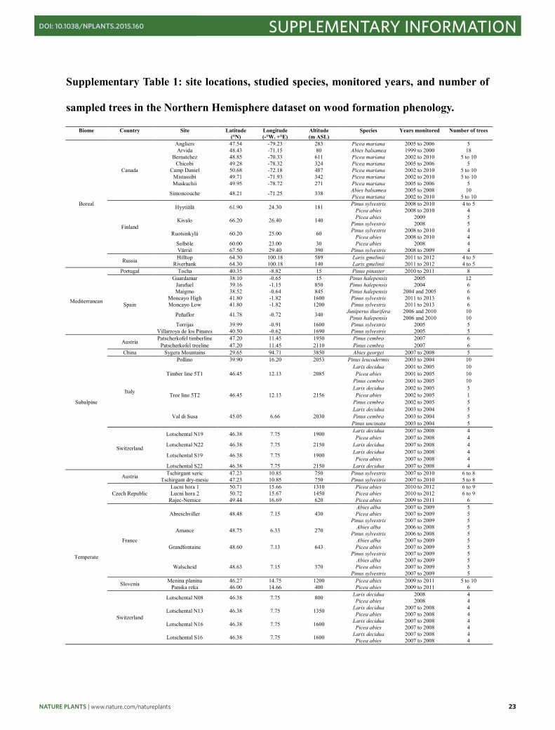
The phenological data collected cover a broad geographical range, with 51 sites spread
from 29.65°N to 67.50°N in latitude, -79.23°W to 100.18°E in longitude, and 15 to 3850 m
ASL in altitude (Supplementary Table 1). Sites were classified in four different forest types
(boreal, Mediterranean, subalpine, and temperate) according to their coordinates and altitudes.
Assessment of the phasing between the seasonal dynamics of xylem size increase, woody
biomass production, and environmental factors
The materials and methods described above allowed us to draw a detailed picture of
the intra-annual dynamics of xylem size increase and woody biomass production, in parallel
to the seasonal course of environmental factors for each studied site, year and species in
northeast France (Supplementary Figs 4, 5, 6). Cross-correlations were performed between
these different time-series in order to assess the degree of synchronisation between the
13
seasonal dynamics of xylem size increase, woody biomass production, and the different
environmental factors. Cross-correlation is a standard method for examining the relationship
between two time series25. It is a measure of similarity of two series as a function of a time-
lag applied to one of them. Therefore, the cross-correlation is helpful for identifying if two
series are synchronised (i.e. the correlation between series is the highest with no time-lag) or
not (i.e. the correlation increases when lagging one of the two series).
We further assessed dependency of xylem size increase and woody biomass
production with the environmental factors using linear models. We focused on the time
window when processes were active (between 5% and 95% of their realisation) in order to
avoid zero values inflation. Within this time window, the intra-annual dynamics of a process
was related to the seasonal course of climatic factors, after removing site and year effects in
order to focus on seasonal variability.
References
1 Granier, A., Breda, N., Biron, P. & Villette, S. A lumped water balance model to
evaluate duration and intensity of drought constraints in forest stands. Ecol. Model.
116, 269-283 (1999).
2 Cuny, H. E. et al. Generalized additive models reveal the intrinsic complexity of wood
formation dynamics. J. Exp. Bot. 64, 1983-1994 (2013).
3 R: A language and environment for statistical computing. R Foundation for Statistical
Computing, Vienna, Austria. ISBN 3-900051-07-0, URL http://www.R-project.org/.
(2015).
NATURE PLANTS | www.nature.com/natureplants 13
SUPPLEMENTARY INFORMATIONDOI: 10.1038/NPLANTS.2015.160
12
observed radial files show at most one last enlarging cell14. The beginning and the cessation of
the period of cell-wall thickening (bW and cW) are computed following the same principles,
but considering wall thickening cells.
On the one hand, the phenology of the cell enlargement period is very similar to the
one of cell division14, and these two processes drive xylem size increase. On the other hand,
because the secondary walls form the bulk of biomass in trees24, the wall thickening process
drives the woody carbon sequestration. Consequently, we considered the phenology of the
periods of cell enlargement and cell-wall thickening as proxies for the timing of xylem size
increase and woody biomass production, respectively. The mean time-lag between xylem size
increase and woody biomass production (Lm) was assessed from the differences observed in
between the beginnings (bE and bW) and the cessations (cW and cE) of the periods of cell
enlargement and cell-wall thickening (Fig. 2):
Lm = (bw−bE)+(cw−cE)2 .
The phenological data collected cover a broad geographical range, with 51 sites spread
from 29.65°N to 67.50°N in latitude, -79.23°W to 100.18°E in longitude, and 15 to 3850 m
ASL in altitude (Supplementary Table 1). Sites were classified in four different forest types
(boreal, Mediterranean, subalpine, and temperate) according to their coordinates and altitudes.
Assessment of the phasing between the seasonal dynamics of xylem size increase, woody
biomass production, and environmental factors
The materials and methods described above allowed us to draw a detailed picture of
the intra-annual dynamics of xylem size increase and woody biomass production, in parallel
to the seasonal course of environmental factors for each studied site, year and species in
northeast France (Supplementary Figs 4, 5, 6). Cross-correlations were performed between
these different time-series in order to assess the degree of synchronisation between the
13
seasonal dynamics of xylem size increase, woody biomass production, and the different
environmental factors. Cross-correlation is a standard method for examining the relationship
between two time series25. It is a measure of similarity of two series as a function of a time-
lag applied to one of them. Therefore, the cross-correlation is helpful for identifying if two
series are synchronised (i.e. the correlation between series is the highest with no time-lag) or
not (i.e. the correlation increases when lagging one of the two series).
We further assessed dependency of xylem size increase and woody biomass
production with the environmental factors using linear models. We focused on the time
window when processes were active (between 5% and 95% of their realisation) in order to
avoid zero values inflation. Within this time window, the intra-annual dynamics of a process
was related to the seasonal course of climatic factors, after removing site and year effects in
order to focus on seasonal variability.
References
1 Granier, A., Breda, N., Biron, P. & Villette, S. A lumped water balance model to
evaluate duration and intensity of drought constraints in forest stands. Ecol. Model.
116, 269-283 (1999).
2 Cuny, H. E. et al. Generalized additive models reveal the intrinsic complexity of wood
formation dynamics. J. Exp. Bot. 64, 1983-1994 (2013).
3 R: A language and environment for statistical computing. R Foundation for Statistical
Computing, Vienna, Austria. ISBN 3-900051-07-0, URL http://www.R-project.org/.
(2015).

14 NATURE PLANTS | www.nature.com/natureplants
SUPPLEMENTARY INFORMATION DOI: 10.1038/NPLANTS.2015.160
14
4 Wood, S. N. Generalized additive models: an introduction with R. (Chapman and
Hall/CRC, 2006).
5 Rossi, S., Anfodillo, T. & Menardi, R. Trephor: a new tool for sampling microcores
from tree stems. Iawa Journal 27, 89-97 (2006).
6 Forster, T., Schweingruber, F. H. & Denneler, B. Increment puncher: a tool for
extracting small cores of wood and bark from living trees. Iawa Journal 21, 169-180
(2000).
7 Deslauriers, A., Morin, H. & Begin, Y. Cellular phenology of annual ring formation of
Abies balsamea in the Quebec boreal forest (Canada). Can. J. For. Res. 33, 190-200
(2003).
8 Cosgrove, D. J. Expansive growth of plant cell walls. Plant Physiol. Biochem. 38,
109-124 (2000).
9 Mellerowicz, E. J., Baucher, M., Sundberg, B. & Boerjan, W. Unravelling cell wall
formation in the woody dicot stem. Plant Mol. Biol. 47, 239-274,
doi:10.1023/a:1010699919325 (2001).
10 Donaldson, L. A. Lignification and lignin topochemistry—an ultrastructural view.
Phytochemistry 57, 859-873 (2001).
15
11 Abe, H., Funada, R., Ohtani, J. & Fukazawa, K. Changes in the arrangement of
cellulose microfibrils associated with the cessation of cell expansion in tracheids.
Trees-Struct. Funct. 11, 328-332 (1997).
12 Kutscha, N. P., Hyland, F. & Schwarzmann, J. M. Certain seasonal changes in balsam
fir cambium and its derivatives. Wood Sci. Technol. 9, 175-188 (1975).
13 Rossi, S., Deslauriers, A. & Morin, H. Application of the Gompertz equation for the
study of xylem cell development. Dendrochronologia 21, 33-39 (2003).
14 Rathgeber, C. B. K., Longuetaud, F., Mothe, F., Cuny, H. & Le Moguedec, G.
Phenology of wood formation: Data processing, analysis and visualisation using R
(package CAVIAR). Dendrochronologia 29, 139-149 (2011).
15 Cuny, H. E., Rathgeber, C. B. K., Frank, D., Fonti, P. & Fournier, M. Kinetics of
tracheid development explain conifer tree-ring structure. New Phytol.,
doi:10.1111/nph.12871 (2014).
16 Hastie, T. & Tibshirani, R. Generalized additive models. Statistical Science 1, 297-318
(1986).
17 McCullagh, P. & Nelder, J. A. Generalized Linear Models. (Chapman and Hall,
1983).
18 Zuur, A. F., Ieno, E. N., Walker, N. J., Saveliev, A. A. & Smith, G. M. Mixed effects
models and extensions in ecology with R. (Springer-Verlag, 2009).
NATURE PLANTS | www.nature.com/natureplants 15
SUPPLEMENTARY INFORMATIONDOI: 10.1038/NPLANTS.2015.160
14
4 Wood, S. N. Generalized additive models: an introduction with R. (Chapman and
Hall/CRC, 2006).
5 Rossi, S., Anfodillo, T. & Menardi, R. Trephor: a new tool for sampling microcores
from tree stems. Iawa Journal 27, 89-97 (2006).
6 Forster, T., Schweingruber, F. H. & Denneler, B. Increment puncher: a tool for
extracting small cores of wood and bark from living trees. Iawa Journal 21, 169-180
(2000).
7 Deslauriers, A., Morin, H. & Begin, Y. Cellular phenology of annual ring formation of
Abies balsamea in the Quebec boreal forest (Canada). Can. J. For. Res. 33, 190-200
(2003).
8 Cosgrove, D. J. Expansive growth of plant cell walls. Plant Physiol. Biochem. 38,
109-124 (2000).
9 Mellerowicz, E. J., Baucher, M., Sundberg, B. & Boerjan, W. Unravelling cell wall
formation in the woody dicot stem. Plant Mol. Biol. 47, 239-274,
doi:10.1023/a:1010699919325 (2001).
10 Donaldson, L. A. Lignification and lignin topochemistry—an ultrastructural view.
Phytochemistry 57, 859-873 (2001).
15
11 Abe, H., Funada, R., Ohtani, J. & Fukazawa, K. Changes in the arrangement of
cellulose microfibrils associated with the cessation of cell expansion in tracheids.
Trees-Struct. Funct. 11, 328-332 (1997).
12 Kutscha, N. P., Hyland, F. & Schwarzmann, J. M. Certain seasonal changes in balsam
fir cambium and its derivatives. Wood Sci. Technol. 9, 175-188 (1975).
13 Rossi, S., Deslauriers, A. & Morin, H. Application of the Gompertz equation for the
study of xylem cell development. Dendrochronologia 21, 33-39 (2003).
14 Rathgeber, C. B. K., Longuetaud, F., Mothe, F., Cuny, H. & Le Moguedec, G.
Phenology of wood formation: Data processing, analysis and visualisation using R
(package CAVIAR). Dendrochronologia 29, 139-149 (2011).
15 Cuny, H. E., Rathgeber, C. B. K., Frank, D., Fonti, P. & Fournier, M. Kinetics of
tracheid development explain conifer tree-ring structure. New Phytol.,
doi:10.1111/nph.12871 (2014).
16 Hastie, T. & Tibshirani, R. Generalized additive models. Statistical Science 1, 297-318
(1986).
17 McCullagh, P. & Nelder, J. A. Generalized Linear Models. (Chapman and Hall,
1983).
18 Zuur, A. F., Ieno, E. N., Walker, N. J., Saveliev, A. A. & Smith, G. M. Mixed effects
models and extensions in ecology with R. (Springer-Verlag, 2009).
16 NATURE PLANTS | www.nature.com/natureplants
SUPPLEMENTARY INFORMATION DOI: 10.1038/NPLANTS.2015.160
16
19 Yee, T. W. & Mitchell, N. D. Generalized additive models in plant ecology. J. Veg.
Sci. 2, 587-602, doi:10.2307/3236170 (1991).
20 Zauer, M., Pfriem, A. & Wagenführ, A. Toward improved understanding of the cell-
wall density and porosity of wood determined by gas pycnometry. Wood Sci. Technol.
47, 1197-1211 (2013).
21 Plötze, M. & Niemz, P. Porosity and pore size distribution of different wood types as
determined by mercury intrusion porosimetry. Eur. J. Wood Wood Prod. 69, 649-657
(2011).
22 Pfriem, A., Zauer, M. & Wagenführ, A. Alteration of the pore structure of spruce
(Picea abies (L.) Karst.) and maple (Acer pseudoplatanus L.) due to thermal treatment
as determined by helium pycnometry and mercury intrusion porosimetry.
Holzforschung 63, 94-98 (2009).
23 Lamlom, S. & Savidge, R. A reassessment of carbon content in wood: variation within
and between 41 North American species. Biomass Bioenergy 25, 381-388 (2003).
24 Zhong, R. & Zheng-Hua, Y. Secondary cell walls. Encyclopedia of Life Sciences
(2009).
25 Chatfield, C. The analysis of time series: an introduction. 6 edn, (Chapman &
Hall/CRC Press, 2003).
17
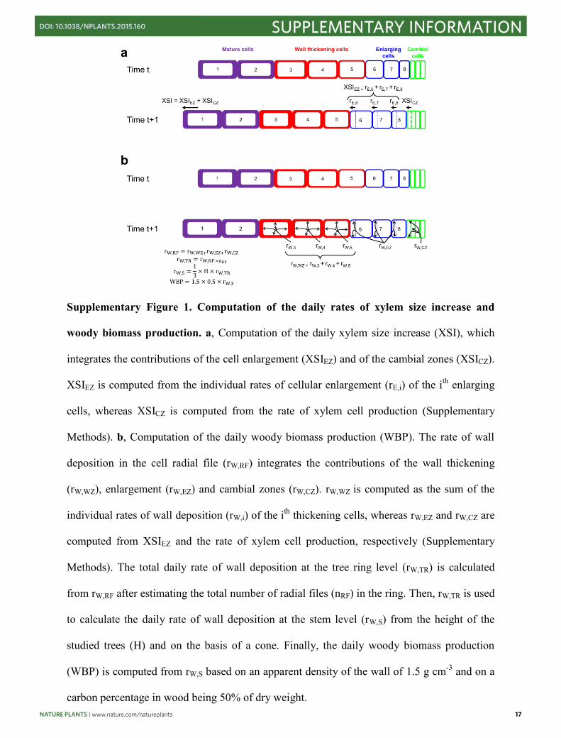
Supplementary Figure 1. Computation of the daily rates of xylem size increase and
woody biomass production. a, Computation of the daily xylem size increase (XSI), which
integrates the contributions of the cell enlargement (XSIEZ) and of the cambial zones (XSICZ).
XSIEZ is computed from the individual rates of cellular enlargement (rE,i) of the ith enlarging
cells, whereas XSICZ is computed from the rate of xylem cell production (Supplementary
Methods). b, Computation of the daily woody biomass production (WBP). The rate of wall
deposition in the cell radial file (rW,RF) integrates the contributions of the wall thickening
(rW,WZ), enlargement (rW,EZ) and cambial zones (rW,CZ). rW,WZ is computed as the sum of the
individual rates of wall deposition (rW,i) of the ith thickening cells, whereas rW,EZ and rW,CZ are
computed from XSIEZ and the rate of xylem cell production, respectively (Supplementary
Methods). The total daily rate of wall deposition at the tree ring level (rW,TR) is calculated
from rW,RF after estimating the total number of radial files (nRF) in the ring. Then, rW,TR is used
to calculate the daily rate of wall deposition at the stem level (rW,S) from the height of the
studied trees (H) and on the basis of a cone. Finally, the daily woody biomass production
(WBP) is computed from rW,S based on an apparent density of the wall of 1.5 g cm-3 and on a
carbon percentage in wood being 50% of dry weight.
NATURE PLANTS | www.nature.com/natureplants 17
SUPPLEMENTARY INFORMATIONDOI: 10.1038/NPLANTS.2015.160
16
19 Yee, T. W. & Mitchell, N. D. Generalized additive models in plant ecology. J. Veg.
Sci. 2, 587-602, doi:10.2307/3236170 (1991).
20 Zauer, M., Pfriem, A. & Wagenführ, A. Toward improved understanding of the cell-
wall density and porosity of wood determined by gas pycnometry. Wood Sci. Technol.
47, 1197-1211 (2013).
21 Plötze, M. & Niemz, P. Porosity and pore size distribution of different wood types as
determined by mercury intrusion porosimetry. Eur. J. Wood Wood Prod. 69, 649-657
(2011).
22 Pfriem, A., Zauer, M. & Wagenführ, A. Alteration of the pore structure of spruce
(Picea abies (L.) Karst.) and maple (Acer pseudoplatanus L.) due to thermal treatment
as determined by helium pycnometry and mercury intrusion porosimetry.
Holzforschung 63, 94-98 (2009).
23 Lamlom, S. & Savidge, R. A reassessment of carbon content in wood: variation within
and between 41 North American species. Biomass Bioenergy 25, 381-388 (2003).
24 Zhong, R. & Zheng-Hua, Y. Secondary cell walls. Encyclopedia of Life Sciences
(2009).
25 Chatfield, C. The analysis of time series: an introduction. 6 edn, (Chapman &
Hall/CRC Press, 2003).
17
Supplementary Figure 1. Computation of the daily rates of xylem size increase and
woody biomass production. a, Computation of the daily xylem size increase (XSI), which
integrates the contributions of the cell enlargement (XSIEZ) and of the cambial zones (XSICZ).
XSIEZ is computed from the individual rates of cellular enlargement (rE,i) of the ith enlarging
cells, whereas XSICZ is computed from the rate of xylem cell production (Supplementary
Methods). b, Computation of the daily woody biomass production (WBP). The rate of wall
deposition in the cell radial file (rW,RF) integrates the contributions of the wall thickening
(rW,WZ), enlargement (rW,EZ) and cambial zones (rW,CZ). rW,WZ is computed as the sum of the
individual rates of wall deposition (rW,i) of the ith thickening cells, whereas rW,EZ and rW,CZ are
computed from XSIEZ and the rate of xylem cell production, respectively (Supplementary
Methods). The total daily rate of wall deposition at the tree ring level (rW,TR) is calculated
from rW,RF after estimating the total number of radial files (nRF) in the ring. Then, rW,TR is used
to calculate the daily rate of wall deposition at the stem level (rW,S) from the height of the
studied trees (H) and on the basis of a cone. Finally, the daily woody biomass production
(WBP) is computed from rW,S based on an apparent density of the wall of 1.5 g cm-3 and on a
carbon percentage in wood being 50% of dry weight.
18 NATURE PLANTS | www.nature.com/natureplants
SUPPLEMENTARY INFORMATION DOI: 10.1038/NPLANTS.2015.160
18
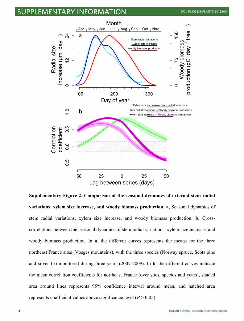
Supplementary Figure 2. Comparison of the seasonal dynamics of external stem radial
variations, xylem size increase, and woody biomass production. a, Seasonal dynamics of
stem radial variations, xylem size increase, and woody biomass production. b, Cross-
correlations between the seasonal dynamics of stem radial variations, xylem size increase, and
woody biomass production. In a, the different curves represents the means for the three
northeast France sites (Vosges mountains), with the three species (Norway spruce, Scots pine
and silver fir) monitored during three years (2007-2009). In b, the different curves indicate
the mean correlation coefficients for northeast France (over sites, species and years), shaded
area around lines represents 95% confidence interval around mean, and hatched area
represents coefficient values above significance level (P > 0.05).
19
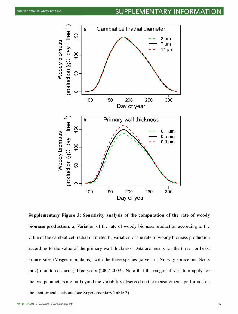
Supplementary Figure 3: Sensitivity analysis of the computation of the rate of woody
biomass production. a, Variation of the rate of woody biomass production according to the
value of the cambial cell radial diameter. b, Variation of the rate of woody biomass production
according to the value of the primary wall thickness. Data are means for the three northeast
France sites (Vosges mountains), with the three species (silver fir, Norway spruce and Scots
pine) monitored during three years (2007-2009). Note that the ranges of variation apply for
the two parameters are far beyond the variability observed on the measurements performed on
the anatomical sections (see Supplementary Table 3).
NATURE PLANTS | www.nature.com/natureplants 19
SUPPLEMENTARY INFORMATIONDOI: 10.1038/NPLANTS.2015.160
18
Supplementary Figure 2. Comparison of the seasonal dynamics of external stem radial
variations, xylem size increase, and woody biomass production. a, Seasonal dynamics of
stem radial variations, xylem size increase, and woody biomass production. b, Cross-
correlations between the seasonal dynamics of stem radial variations, xylem size increase, and
woody biomass production. In a, the different curves represents the means for the three
northeast France sites (Vosges mountains), with the three species (Norway spruce, Scots pine
and silver fir) monitored during three years (2007-2009). In b, the different curves indicate
the mean correlation coefficients for northeast France (over sites, species and years), shaded
area around lines represents 95% confidence interval around mean, and hatched area
represents coefficient values above significance level (P > 0.05).
19
Supplementary Figure 3: Sensitivity analysis of the computation of the rate of woody
biomass production. a, Variation of the rate of woody biomass production according to the
value of the cambial cell radial diameter. b, Variation of the rate of woody biomass production
according to the value of the primary wall thickness. Data are means for the three northeast
France sites (Vosges mountains), with the three species (silver fir, Norway spruce and Scots
pine) monitored during three years (2007-2009). Note that the ranges of variation apply for
the two parameters are far beyond the variability observed on the measurements performed on
the anatomical sections (see Supplementary Table 3).
20 NATURE PLANTS | www.nature.com/natureplants
SUPPLEMENTARY INFORMATION DOI: 10.1038/NPLANTS.2015.160
20
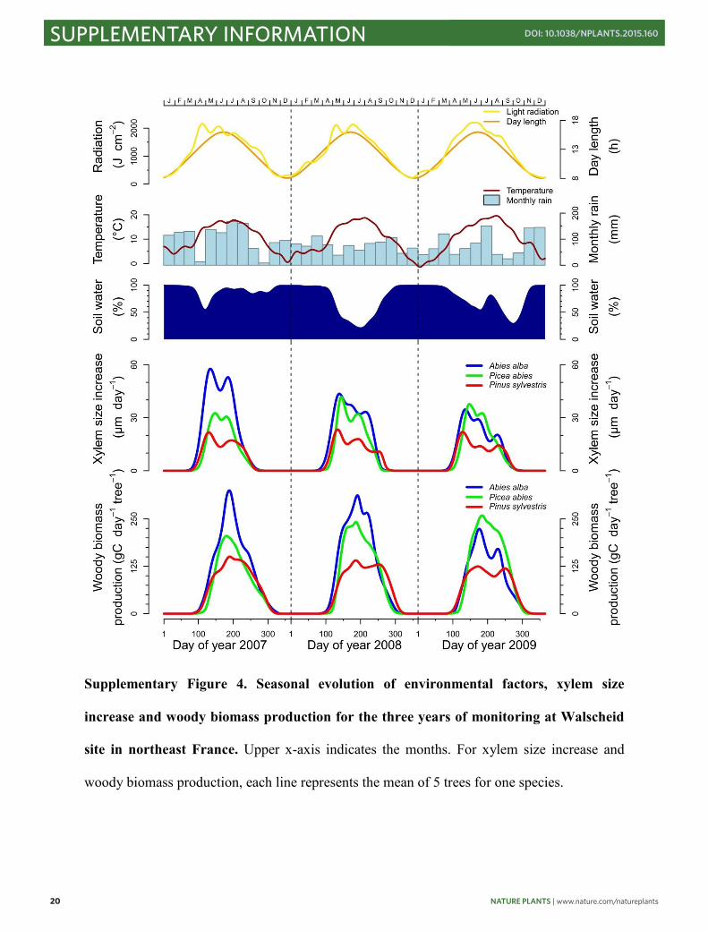
Supplementary Figure 4. Seasonal evolution of environmental factors, xylem size
increase and woody biomass production for the three years of monitoring at Walscheid
site in northeast France. Upper x-axis indicates the months. For xylem size increase and
woody biomass production, each line represents the mean of 5 trees for one species.
21
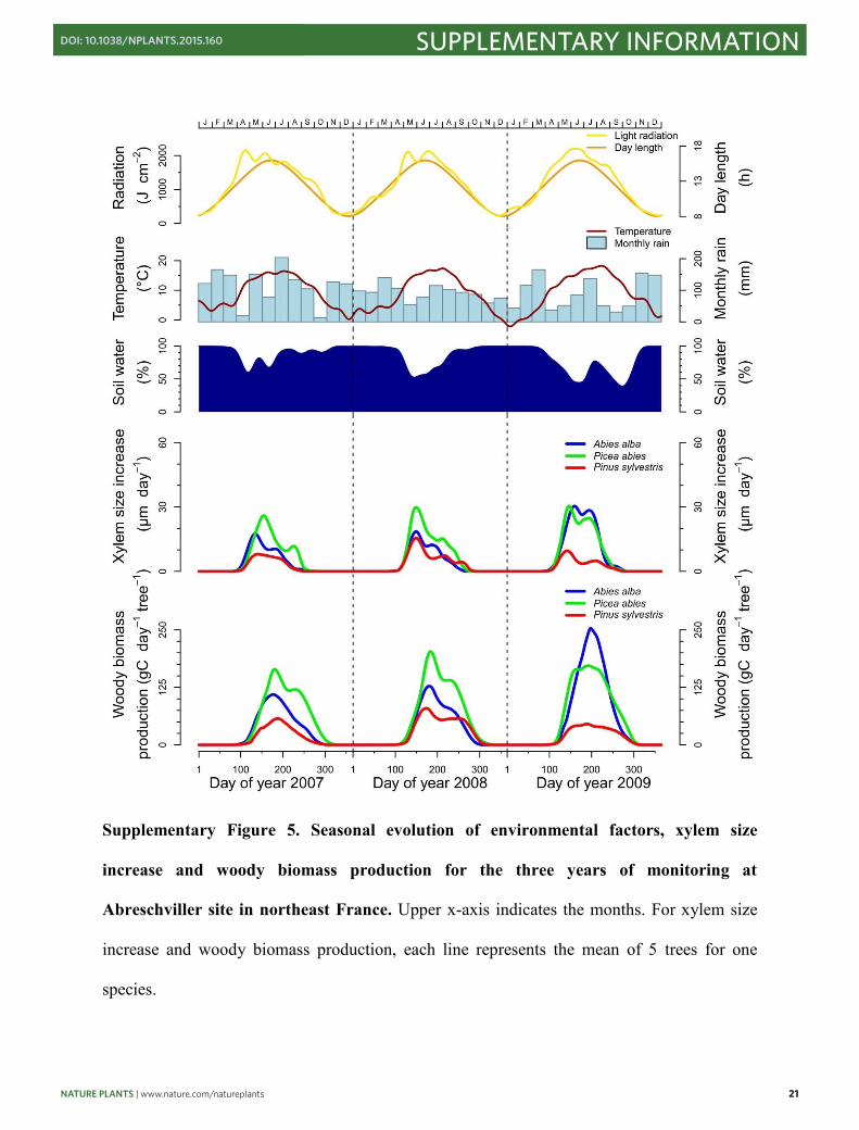
Supplementary Figure 5. Seasonal evolution of environmental factors, xylem size
increase and woody biomass production for the three years of monitoring at
Abreschviller site in northeast France. Upper x-axis indicates the months. For xylem size
increase and woody biomass production, each line represents the mean of 5 trees for one
species.
NATURE PLANTS | www.nature.com/natureplants 21
SUPPLEMENTARY INFORMATIONDOI: 10.1038/NPLANTS.2015.160
20
Supplementary Figure 4. Seasonal evolution of environmental factors, xylem size
increase and woody biomass production for the three years of monitoring at Walscheid
site in northeast France. Upper x-axis indicates the months. For xylem size increase and
woody biomass production, each line represents the mean of 5 trees for one species.
21
Supplementary Figure 5. Seasonal evolution of environmental factors, xylem size
increase and woody biomass production for the three years of monitoring at
Abreschviller site in northeast France. Upper x-axis indicates the months. For xylem size
increase and woody biomass production, each line represents the mean of 5 trees for one
species.
22 NATURE PLANTS | www.nature.com/natureplants
SUPPLEMENTARY INFORMATION DOI: 10.1038/NPLANTS.2015.160
22
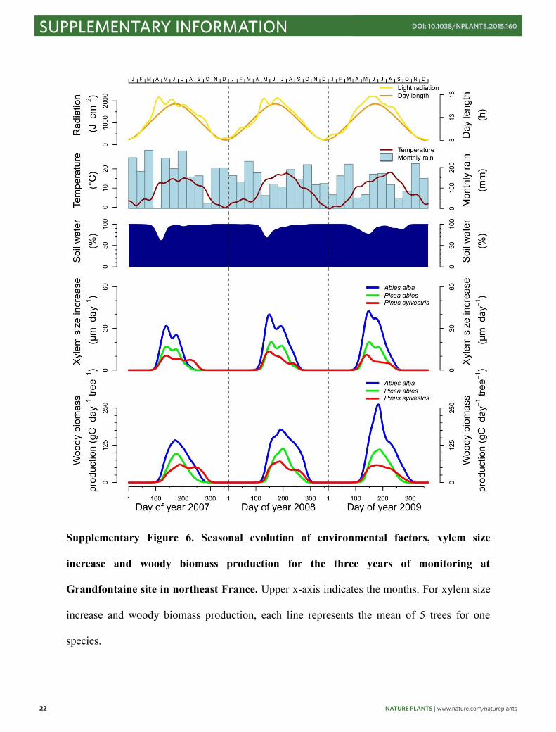
Supplementary Figure 6. Seasonal evolution of environmental factors, xylem size
increase and woody biomass production for the three years of monitoring at
Grandfontaine site in northeast France. Upper x-axis indicates the months. For xylem size
increase and woody biomass production, each line represents the mean of 5 trees for one
species.
23
Supplementary Table 1: site locations, studied species, monitored years, and number of
sampled trees in the Northern Hemisphere dataset on wood formation phenology.
Biome Country Site Latitude (°N)
Longitude (-°W. +°E)
Altitude (m ASL)
Species Years monitored Number of trees
Boreal
Canada
Angliers 47.54 -79.23 283 Picea mariana 2005 to 2006 5 Arvida 48.43 -71.15 80 Abies balsamea 1999 to 2000 18
Bernatchez 48.85 -70.33 611 Picea mariana 2002 to 2010 5 to 10 Chicobi 49.28 -78.32 324 Picea mariana 2005 to 2006 5
Camp Daniel 50.68 -72.18 487 Picea mariana 2002 to 2010 5 to 10 Mistassibi 49.71 -71.93 342 Picea mariana 2002 to 2010 5 to 10 Muskuchii 49.95 -78.72 271 Picea mariana 2005 to 2006 5
Simoncouche 48.21 -71.25 338 Abies balsamea 2005 to 2008 10 Picea mariana 2002 to 2010 5 to 10
Finland
Hyytiälä 61.90 24.30 181 Pinus sylvestris 2008 to 2010 4 to 5 Picea abies 2008 to 2010 4
Kivalo 66.20 26.40 140 Picea abies 2009 5 Pinus sylvestris 2008 5
Ruotsinkylä 60.20 25.00 60 Pinus sylvestris 2008 to 2010 4 Picea abies 2008 to 2010 4
Solböle 60.00 23.00 30 Picea abies 2008 4 Värriö 67.50 29.40 390 Pinus sylvestris 2008 to 2009 4
Russia Hilltop 64.30 100.18 589 Larix gmelinii 2011 to 2012 4 to 5 Riverbank 64.30 100.18 140 Larix gmelinii 2011 to 2012 4 to 5
Mediterranean
Portugal Tocha 40.35 -8.82 15 Pinus pinaster 2010 to 2011 8
Spain
Guardamar 38.10 -0.65 15 Pinus halepensis 2005 12 Jarafuel 39.16 -1.15 850 Pinus halepensis 2004 6 Maigmo 38.52 -0.64 845 Pinus halepensis 2004 and 2005 6
Moncayo High 41.80 -1.82 1600 Pinus sylvestris 2011 to 2013 6 Moncayo Low 41.80 -1.82 1200 Pinus sylvestris 2011 to 2013 6
Peñaflor 41.78 -0.72 340 Juniperus thurifera 2006 and 2010 10 Pinus halepensis 2006 and 2010 10
Torrijas 39.99 -0.91 1600 Pinus sylvestris 2005 5 Villarroya de los Pinares 40.50 -0.62 1690 Pinus sylvestris 2005 5
Subalpine
Austria Patscherkofel timberline 47.20 11.45 1950 Pinus cembra 2007 6 Patscherkofel treeline 47.20 11.45 2110 Pinus cembra 2007 6
China Sygera Mountains 29.65 94.71 3850 Abies georgei 2007 to 2008 5
Italy
Pollino 39.90 16.20 2053 Pinus leucodermis 2003 to 2004 10
Timber line 5T1 46.45 12.13 2085 Larix decidua 2001 to 2005 10 Picea abies 2001 to 2005 10
Pinus cembra 2001 to 2005 10
Tree line 5T2 46.45 12.13 2156 Larix decidua 2002 to 2005 5 Picea abies 2002 to 2005 1
Pinus cembra 2002 to 2005 5
Val di Susa 45.05 6.66 2030 Larix decidua 2003 to 2004 5 Pinus cembra 2003 to 2004 5 Pinus uncinata 2003 to 2004 5
Switzerland
Lotschental N19 46.38 7.75 1900 Larix decidua 2007 to 2008 4 Picea abies 2007 to 2008 4
Lotschental N22 46.38 7.75 2150 Larix decidua 2007 to 2008 4
Lotschental S19 46.38 7.75 1900 Larix decidua 2007 to 2008 4 Picea abies 2007 to 2008 4
Lotschental S22 46.38 7.75 2150 Larix decidua 2007 to 2008 4
Temperate
Austria Tschirgant xeric 47.23 10.85 750 Pinus sylvestris 2007 to 2010 6 to 8 Tschirgant dry-mesic 47.23 10.85 750 Pinus sylvestris 2007 to 2010 5 to 8
Czech Republic Lucni hora 1 50.71 15.66 1310 Picea abies 2010 to 2012 6 to 9 Lucni hora 2 50.72 15.67 1450 Picea abies 2010 to 2012 6 to 9
Rajec-Nemice 49.44 16.69 620 Picea abies 2009 to 2011 6
France
Abreschviller 48.48 7.15 430 Abies alba 2007 to 2009 5 Picea abies 2007 to 2009 5
Pinus sylvestris 2007 to 2009 5
Amance 48.75 6.33 270 Abies alba 2006 to 2008 5 Pinus sylvestris 2006 to 2008 5
Grandfontaine 48.60 7.13 643 Abies alba 2007 to 2009 5 Picea abies 2007 to 2009 5
Pinus sylvestris 2007 to 2009 5
Walscheid 48.63 7.15 370 Abies alba 2007 to 2009 5 Picea abies 2007 to 2009 5
Pinus sylvestris 2007 to 2009 5
Slovenia Menina planina 46.27 14.75 1200 Picea abies 2009 to 2011 5 to 10 Panska reka 46.00 14.66 400 Picea abies 2009 to 2011 6
Switzerland
Lotschental N08 46.38 7.75 800 Larix decidua 2008 4 Picea abies 2008 4
Lotschental N13 46.38 7.75 1350 Larix decidua 2007 to 2008 4 Picea abies 2007 to 2008 4
Lotschental N16 46.38 7.75 1600 Larix decidua 2007 to 2008 4 Picea abies 2007 to 2008 4
Lotschental S16 46.38 7.75 1600 Larix decidua 2007 to 2008 4 Picea abies 2007 to 2008 4
NATURE PLANTS | www.nature.com/natureplants 23
SUPPLEMENTARY INFORMATIONDOI: 10.1038/NPLANTS.2015.160
22
Supplementary Figure 6. Seasonal evolution of environmental factors, xylem size
increase and woody biomass production for the three years of monitoring at
Grandfontaine site in northeast France. Upper x-axis indicates the months. For xylem size
increase and woody biomass production, each line represents the mean of 5 trees for one
species.
23
Supplementary Table 1: site locations, studied species, monitored years, and number of
sampled trees in the Northern Hemisphere dataset on wood formation phenology.
Biome Country Site Latitude (°N)
Longitude (-°W. +°E)
Altitude (m ASL)
Species Years monitored Number of trees
Boreal
Canada
Angliers 47.54 -79.23 283 Picea mariana 2005 to 2006 5 Arvida 48.43 -71.15 80 Abies balsamea 1999 to 2000 18
Bernatchez 48.85 -70.33 611 Picea mariana 2002 to 2010 5 to 10 Chicobi 49.28 -78.32 324 Picea mariana 2005 to 2006 5
Camp Daniel 50.68 -72.18 487 Picea mariana 2002 to 2010 5 to 10 Mistassibi 49.71 -71.93 342 Picea mariana 2002 to 2010 5 to 10 Muskuchii 49.95 -78.72 271 Picea mariana 2005 to 2006 5
Simoncouche 48.21 -71.25 338 Abies balsamea 2005 to 2008 10 Picea mariana 2002 to 2010 5 to 10
Finland
Hyytiälä 61.90 24.30 181 Pinus sylvestris 2008 to 2010 4 to 5 Picea abies 2008 to 2010 4
Kivalo 66.20 26.40 140 Picea abies 2009 5 Pinus sylvestris 2008 5
Ruotsinkylä 60.20 25.00 60 Pinus sylvestris 2008 to 2010 4 Picea abies 2008 to 2010 4
Solböle 60.00 23.00 30 Picea abies 2008 4 Värriö 67.50 29.40 390 Pinus sylvestris 2008 to 2009 4
Russia Hilltop 64.30 100.18 589 Larix gmelinii 2011 to 2012 4 to 5 Riverbank 64.30 100.18 140 Larix gmelinii 2011 to 2012 4 to 5
Mediterranean
Portugal Tocha 40.35 -8.82 15 Pinus pinaster 2010 to 2011 8
Spain
Guardamar 38.10 -0.65 15 Pinus halepensis 2005 12 Jarafuel 39.16 -1.15 850 Pinus halepensis 2004 6 Maigmo 38.52 -0.64 845 Pinus halepensis 2004 and 2005 6
Moncayo High 41.80 -1.82 1600 Pinus sylvestris 2011 to 2013 6 Moncayo Low 41.80 -1.82 1200 Pinus sylvestris 2011 to 2013 6
Peñaflor 41.78 -0.72 340 Juniperus thurifera 2006 and 2010 10 Pinus halepensis 2006 and 2010 10
Torrijas 39.99 -0.91 1600 Pinus sylvestris 2005 5 Villarroya de los Pinares 40.50 -0.62 1690 Pinus sylvestris 2005 5
Subalpine
Austria Patscherkofel timberline 47.20 11.45 1950 Pinus cembra 2007 6 Patscherkofel treeline 47.20 11.45 2110 Pinus cembra 2007 6
China Sygera Mountains 29.65 94.71 3850 Abies georgei 2007 to 2008 5
Italy
Pollino 39.90 16.20 2053 Pinus leucodermis 2003 to 2004 10
Timber line 5T1 46.45 12.13 2085 Larix decidua 2001 to 2005 10 Picea abies 2001 to 2005 10
Pinus cembra 2001 to 2005 10
Tree line 5T2 46.45 12.13 2156 Larix decidua 2002 to 2005 5 Picea abies 2002 to 2005 1
Pinus cembra 2002 to 2005 5
Val di Susa 45.05 6.66 2030 Larix decidua 2003 to 2004 5 Pinus cembra 2003 to 2004 5 Pinus uncinata 2003 to 2004 5
Switzerland
Lotschental N19 46.38 7.75 1900 Larix decidua 2007 to 2008 4 Picea abies 2007 to 2008 4
Lotschental N22 46.38 7.75 2150 Larix decidua 2007 to 2008 4
Lotschental S19 46.38 7.75 1900 Larix decidua 2007 to 2008 4 Picea abies 2007 to 2008 4
Lotschental S22 46.38 7.75 2150 Larix decidua 2007 to 2008 4
Temperate
Austria Tschirgant xeric 47.23 10.85 750 Pinus sylvestris 2007 to 2010 6 to 8 Tschirgant dry-mesic 47.23 10.85 750 Pinus sylvestris 2007 to 2010 5 to 8
Czech Republic Lucni hora 1 50.71 15.66 1310 Picea abies 2010 to 2012 6 to 9 Lucni hora 2 50.72 15.67 1450 Picea abies 2010 to 2012 6 to 9
Rajec-Nemice 49.44 16.69 620 Picea abies 2009 to 2011 6
France
Abreschviller 48.48 7.15 430 Abies alba 2007 to 2009 5 Picea abies 2007 to 2009 5
Pinus sylvestris 2007 to 2009 5
Amance 48.75 6.33 270 Abies alba 2006 to 2008 5 Pinus sylvestris 2006 to 2008 5
Grandfontaine 48.60 7.13 643 Abies alba 2007 to 2009 5 Picea abies 2007 to 2009 5
Pinus sylvestris 2007 to 2009 5
Walscheid 48.63 7.15 370 Abies alba 2007 to 2009 5 Picea abies 2007 to 2009 5
Pinus sylvestris 2007 to 2009 5
Slovenia Menina planina 46.27 14.75 1200 Picea abies 2009 to 2011 5 to 10 Panska reka 46.00 14.66 400 Picea abies 2009 to 2011 6
Switzerland
Lotschental N08 46.38 7.75 800 Larix decidua 2008 4 Picea abies 2008 4
Lotschental N13 46.38 7.75 1350 Larix decidua 2007 to 2008 4 Picea abies 2007 to 2008 4
Lotschental N16 46.38 7.75 1600 Larix decidua 2007 to 2008 4 Picea abies 2007 to 2008 4
Lotschental S16 46.38 7.75 1600 Larix decidua 2007 to 2008 4 Picea abies 2007 to 2008 4
24 NATURE PLANTS | www.nature.com/natureplants
SUPPLEMENTARY INFORMATION DOI: 10.1038/NPLANTS.2015.160
24
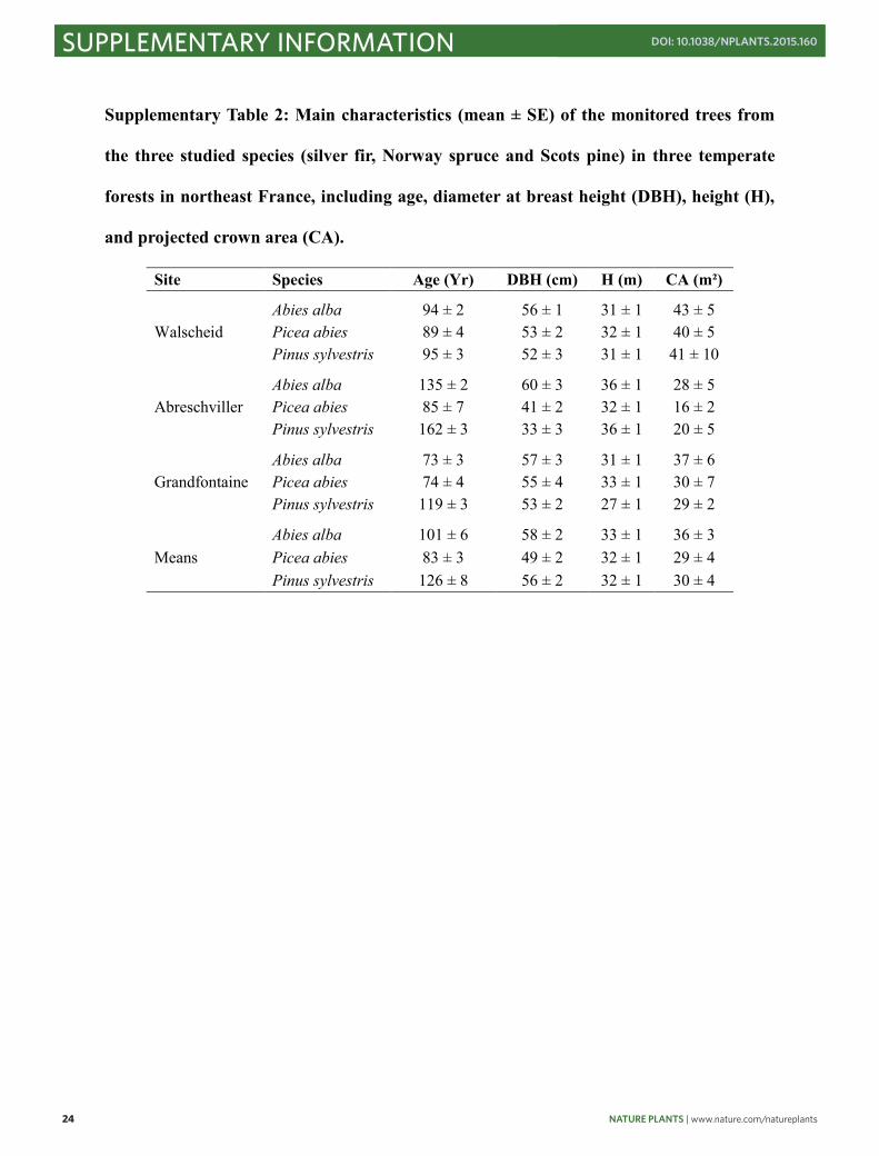
Supplementary Table 2: Main characteristics (mean ± SE) of the monitored trees from
the three studied species (silver fir, Norway spruce and Scots pine) in three temperate
forests in northeast France, including age, diameter at breast height (DBH), height (H),
and projected crown area (CA).
Site Species Age (Yr) DBH (cm) H (m) CA (m²) Walscheid
Abies alba 94 ± 2 56 ± 1 31 ± 1 43 ± 5 Picea abies 89 ± 4 53 ± 2 32 ± 1 40 ± 5 Pinus sylvestris 95 ± 3 52 ± 3 31 ± 1 41 ± 10
Abreschviller
Abies alba 135 ± 2 60 ± 3 36 ± 1 28 ± 5 Picea abies 85 ± 7 41 ± 2 32 ± 1 16 ± 2 Pinus sylvestris 162 ± 3 33 ± 3 36 ± 1 20 ± 5
Grandfontaine
Abies alba 73 ± 3 57 ± 3 31 ± 1 37 ± 6 Picea abies 74 ± 4 55 ± 4 33 ± 1 30 ± 7 Pinus sylvestris 119 ± 3 53 ± 2 27 ± 1 29 ± 2
Means
Abies alba 101 ± 6 58 ± 2 33 ± 1 36 ± 3 Picea abies 83 ± 3 49 ± 2 32 ± 1 29 ± 4 Pinus sylvestris 126 ± 8 56 ± 2 32 ± 1 30 ± 4
25
Supplementary Table 3: Values (means ± standard deviation) of cambial cell radial
diameter and primary wall thickness during the growing season for the different sites,
years, and species in northeast France. Measurements were performed during the growing
season for one tree per site, year, and species, with approximately 40 measurements for each
variable on each sample.
Site Year Species Cambial cell radial diameter
Primary wall thickness
Walscheid
2007 Abies alba 6.7 ± 2.4 0.48 ± 0.12 Picea abies 6.7 ± 1.7 0.50 ± 0.14 Pinus sylvestris 7.0 ± 2.1 0.50 ± 0.08
2008 Abies alba 7.8 ± 2.6 0.56 ± 0.07 Picea abies 7.0 ± 3.9 0.50 ± 0.07 Pinus sylvestris 6.6 ± 4.0 0.51 ± 0.08
2009 Abies alba 7.0 ± 3.2 0.53 ± 0.08 Picea abies 6.7 ± 3.3 0.51 ± 0.10 Pinus sylvestris 7.1 ± 3.6 0.49 ± 0.07
Abreschviller
2007 Abies alba 7.3 ± 2.2 0.49 ± 0.10 Picea abies 6.8 ± 2.8 0.50 ± 0.14 Pinus sylvestris 6.8 ± 2.6 0.56 ± 0.11
2008 Abies alba 6.9 ± 3.0 0.46 ± 0.10 Picea abies 6.9 ± 3.0 0.48 ± 0.07 Pinus sylvestris 7.0 ± 2.3 0.48 ± 0.10
2009 Abies alba 7.0 ± 2.9 0.52 ± 0.07 Picea abies 7.0 ± 3.0 0.46 ± 0.08 Pinus sylvestris 7.3 ± 3.5 0.48 ± 0.08
Grandfontaine
2007 Abies alba 6.9 ± 2.3 0.49 ± 0.11 Picea abies 6.9 ± 2.6 0.47 ± 0.09 Pinus sylvestris 7.0 ± 2.4 0.48 ± 0.09
2008 Abies alba 6.8 ± 2.4 0.54 ± 0.08 Picea abies 6.8 ± 2.2 0.58 ± 0.10 Pinus sylvestris 7.1 ± 2.8 0.50 ± 0.08
2009 Abies alba 7.2 ± 2.2 0.50 ± 0.13 Picea abies 6.9 ± 3.6 0.52 ± 0.14 Pinus sylvestris 6.9 ± 2.8 0.52 ± 0.06
Means 7.0 ± 2.8 0.51 ± 0.09
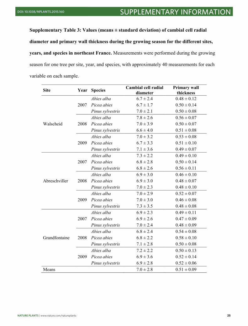
NATURE PLANTS | www.nature.com/natureplants 25
SUPPLEMENTARY INFORMATIONDOI: 10.1038/NPLANTS.2015.160
24
Supplementary Table 2: Main characteristics (mean ± SE) of the monitored trees from
the three studied species (silver fir, Norway spruce and Scots pine) in three temperate
forests in northeast France, including age, diameter at breast height (DBH), height (H),
and projected crown area (CA).
Site Species Age (Yr) DBH (cm) H (m) CA (m²) Walscheid
Abies alba 94 ± 2 56 ± 1 31 ± 1 43 ± 5 Picea abies 89 ± 4 53 ± 2 32 ± 1 40 ± 5 Pinus sylvestris 95 ± 3 52 ± 3 31 ± 1 41 ± 10
Abreschviller
Abies alba 135 ± 2 60 ± 3 36 ± 1 28 ± 5 Picea abies 85 ± 7 41 ± 2 32 ± 1 16 ± 2 Pinus sylvestris 162 ± 3 33 ± 3 36 ± 1 20 ± 5
Grandfontaine
Abies alba 73 ± 3 57 ± 3 31 ± 1 37 ± 6 Picea abies 74 ± 4 55 ± 4 33 ± 1 30 ± 7 Pinus sylvestris 119 ± 3 53 ± 2 27 ± 1 29 ± 2
Means
Abies alba 101 ± 6 58 ± 2 33 ± 1 36 ± 3 Picea abies 83 ± 3 49 ± 2 32 ± 1 29 ± 4 Pinus sylvestris 126 ± 8 56 ± 2 32 ± 1 30 ± 4
25
Supplementary Table 3: Values (means ± standard deviation) of cambial cell radial
diameter and primary wall thickness during the growing season for the different sites,
years, and species in northeast France. Measurements were performed during the growing
season for one tree per site, year, and species, with approximately 40 measurements for each
variable on each sample.
Site Year Species Cambial cell radial diameter
Primary wall thickness
Walscheid
2007 Abies alba 6.7 ± 2.4 0.48 ± 0.12 Picea abies 6.7 ± 1.7 0.50 ± 0.14 Pinus sylvestris 7.0 ± 2.1 0.50 ± 0.08
2008 Abies alba 7.8 ± 2.6 0.56 ± 0.07 Picea abies 7.0 ± 3.9 0.50 ± 0.07 Pinus sylvestris 6.6 ± 4.0 0.51 ± 0.08
2009 Abies alba 7.0 ± 3.2 0.53 ± 0.08 Picea abies 6.7 ± 3.3 0.51 ± 0.10 Pinus sylvestris 7.1 ± 3.6 0.49 ± 0.07
Abreschviller
2007 Abies alba 7.3 ± 2.2 0.49 ± 0.10 Picea abies 6.8 ± 2.8 0.50 ± 0.14 Pinus sylvestris 6.8 ± 2.6 0.56 ± 0.11
2008 Abies alba 6.9 ± 3.0 0.46 ± 0.10 Picea abies 6.9 ± 3.0 0.48 ± 0.07 Pinus sylvestris 7.0 ± 2.3 0.48 ± 0.10
2009 Abies alba 7.0 ± 2.9 0.52 ± 0.07 Picea abies 7.0 ± 3.0 0.46 ± 0.08 Pinus sylvestris 7.3 ± 3.5 0.48 ± 0.08
Grandfontaine
2007 Abies alba 6.9 ± 2.3 0.49 ± 0.11 Picea abies 6.9 ± 2.6 0.47 ± 0.09 Pinus sylvestris 7.0 ± 2.4 0.48 ± 0.09
2008 Abies alba 6.8 ± 2.4 0.54 ± 0.08 Picea abies 6.8 ± 2.2 0.58 ± 0.10 Pinus sylvestris 7.1 ± 2.8 0.50 ± 0.08
2009 Abies alba 7.2 ± 2.2 0.50 ± 0.13 Picea abies 6.9 ± 3.6 0.52 ± 0.14 Pinus sylvestris 6.9 ± 2.8 0.52 ± 0.06
Means 7.0 ± 2.8 0.51 ± 0.09