Supplementary Information for Ultra-Large-Scale … · Supplementary Information for...

SUPPLEMENTARY INFORMATIONDOI: 10.1038/NPHOTON.2013.287

NATURE PHOTONICS | www.nature.com/naturephotonics 1

Supplementary Information forUltra-Large-Scale Continuous-Variable Cluster States

Multiplexed in the Time Domain

S1 Experimental Setup

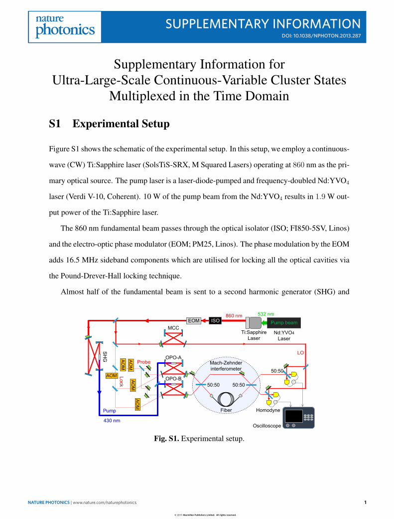
Figure S1 shows the schematic of the experimental setup. In this setup, we employ a continuous-

wave (CW) Ti:Sapphire laser (SolsTiS-SRX, M Squared Lasers) operating at 860 nm as the pri-

mary optical source. The pump laser is a laser-diode-pumped and frequency-doubled Nd:YVO4

laser (Verdi V-10, Coherent). 10 W of the pump beam from the Nd:YVO4 results in 1.9 W out-

put power of the Ti:Sapphire laser.

The 860 nm fundamental beam passes through the optical isolator (ISO; FI850-5SV, Linos)

and the electro-optic phase modulator (EOM; PM25, Linos). The phase modulation by the EOM

adds 16.5 MHz sideband components which are utilised for locking all the optical cavities via

the Pound-Drever-Hall locking technique.

Almost half of the fundamental beam is sent to a second harmonic generator (SHG) and

860 nm 532 nm

Pump beam

Nd:YVO4Laser

Ti:SapphireLaser

ISOEOMMCC

430 nm

Pump

Lock

OPO-A

OPO-B

Mach-Zehnderinterferometer

Probe

AOM

AO

M

AO

MA

OM

AO

M

Fiber

50:50 50:50

Homodyne

Oscilloscope

50:50

LOSH

G

Fig. S1. Experimental setup.

1

© 2013 Macmillan Publishers Limited. All rights reserved.

2 NATURE PHOTONICS | www.nature.com/naturephotonics

SUPPLEMENTARY INFORMATION DOI: 10.1038/NPHOTON.2013.287

converted to approximately 500 mW of a 430 nm beam. The SHG is a bow-tie cavity consisting

of two spherical mirrors (radius of curvature 50 mm), two flat mirrors, and contains a 10 mm

× 3 mm × 3 mm KNbO3 crystal. Its round trip length is 500 mm, and the input coupler

transmissivity is 10%. The rest of the fundamental beam is further split and distributed for

controlling the sub-threshold optical parametric oscillators (OPOs), the interferometers, the

homodyne detectors, and so on.

The second harmonic from the SHG is injected into the OPOs as their pump beam (100 mW

for each OPO) to generate the squeezed vacuum beams, which are the quantum resources for

this experiment. The OPO is a bow-tie cavity consisting of two spherical mirrors (radius of

curvature 38 mm), two flat mirrors and a 10 mm × 1 mm × 1 mm periodically poled KTiOPO4

(PPKTP) crystal. Its round trip length is 230 mm, the half width at half maximum is 17 MHz,

the output coupler transmissivities are 14.9% (OPO-A) and 15.4% (OPO-B), and intra cavity

losses are 0.41% (OPO-A) and 0.30% (OPO-B). The OPO is locked via the Pound-Drever-Hall

locking method by introducing a locking beam which is appropriately frequency-shifted and

counter-propagating in the cavity so as to avoid interference with the squeezed vacuum beam.

The squeezed vacuum states are combined by a Mach-Zehnder interferometer (MZI) with

asymmetric arm lengths. After the first balanced beam-splitter, they are converted into two-

mode EPR states. The EPR states become staggered due to the asymmetric arm lengths. The

staggered EPR states are then combined in sequence at the second balanced beam-splitter, form-

ing the extended EPR state.

For the optical delay line to asymmetrise the MZI, we employ an optical fiber. To minimize

the insertion loss of the delay line, we employ fiber patchcodes with special anti-reflection

(AR) coatings at 860 nm on both ends (PMJ-3A3A-850-5/125-1-2-1-AR2, OZ Optics). We

fabricated arbitrary lengths of fiber cables by splicing the patchcodes and bare fibers (SM85-

PS-U40A, Fujikura). The lenses for focusing and collimating the beam are single aspheric

2




lenses with AR coatings (C240TME-B, Thorlabs). Furthermore, in the aim of improving the

spatial mode matching between the TEM00 in free-space and LP01 in PM fibers, we developed

a special fiber alignment device (FA1000S, FMD Corporation). As a result, we obtained 92%

in the throughput of the entire fiber delay line, which was kept as high as 89% during 6 hours.

Since small temperature changes around the fiber cause drastic changes of the optical pass

length resulting in the instability of phase locking, the fiber is placed inside a box consisting of

heat insulating material and vibration-proofing materials.

The Extended EPR states are measured by homodyne detectors. The two homodyne mea-

surements are performed with balanced beam-splitters and continuous-wave local oscillator

(LO) beams. To optimise the spatial mode-matching, the LO beams are first filtered by a sep-

arate cavity which is a bow-tie cavity consisting of two spherical mirrors (radius of curvature

38 mm) and two flat mirrors. Its round trip is 230 mm length, finesse is 25, the half width at half

maximum is 27 MHz, and the input and output coupler transmissivities are both 5%. Visibili-

ties are above 98% for every pair of signal beams through free space including the LO beams.

The average visibility through the fiber is 95%. The propagation efficiencies from the OPOs to

the homodyne detectors are 85–96%. The quantum efficiencies of photodiodes (special order,

Hamamatsu Photonics) used in homodyne detectors are about 99%, while the bandwidth of the

detectors are above 20 MHz. The LO power is set to 10 mW for every homodyne measurement.

The signals from the homodyne detectors in the time-domain are stored by an oscilloscope

(DPO 7054, Tektronix). The sampling rate of the oscilloscope is set to 200 MHz in order to

sample enough data points in each wave packet. Each frame of 2.5 ms contains 500, 000 points,

corresponding to about 30, 000 wave-packets. For each quadrature measurement of each wave-

packet we measure 3, 000 frames in order to gather enough statistics to calculate variances. The

3




quadrature amplitudes are elicited from them by using the temporal mode function f(t).

ξk =

∫ T/2

−T/2

ξ(t− kT )f(t)dt, (S1)

where ξk (ξ = x, p) are discretized quadratures, ξ(t) (ξ = x, p) are continuous quadratures

from the homodyne detectors, and f(t) is a Gaussian filter f(t) ∝ e−(Γt)2 which is normalised

as∫ T/2

−T/2|f(t)|2 dt = 1. While the bandwidth Γ can be chosen arbitrarily, the interval of the

wave-packet T depends on the fiber length. The parameters used here are T = 157.5 ns and

Γ = 2π × 2.5 MHz (1/Γ ∼ 64 ns).

It is necessary to lock the relative phases of beams at every point where the beams interfere.

For this purpose, we utilise bright laser beams of about 10 µW, which are directed by homodyne

detectors. However, their laser noise interferes with our measurement results. To avoid this

problem, we switch between data acquisition and feedback control periodically at a switching

frequency of 25 Hz. Furthermore, to realise strong and reliable phase locking, we implement

a custom-made digital feedback control system via field programmable gate arrays (NI PXI-

7853R, National Instruments) in PXI chassis (NI PXI-1033, National Instruments).

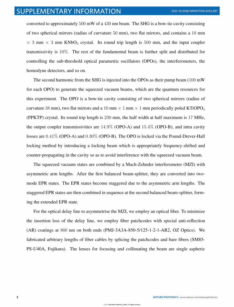
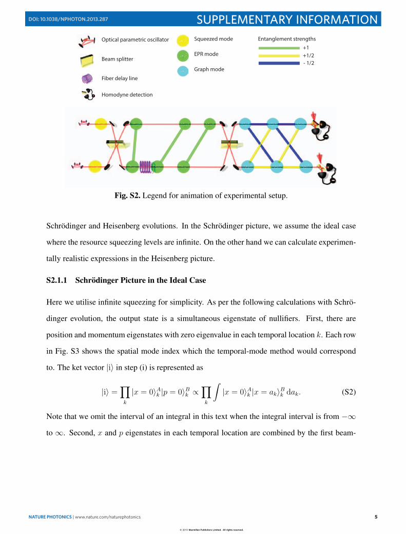
S1.1 Animation

An animation can be found at (http://www.alice.t.u-tokyo.ac.jp/Graph-animation.avi) that shows

temporal modes propagating through the experimental setup. Figure S2 is provided as a legend

for the animation.

S2 Theory

S2.1 Derivation of Extended EPR States

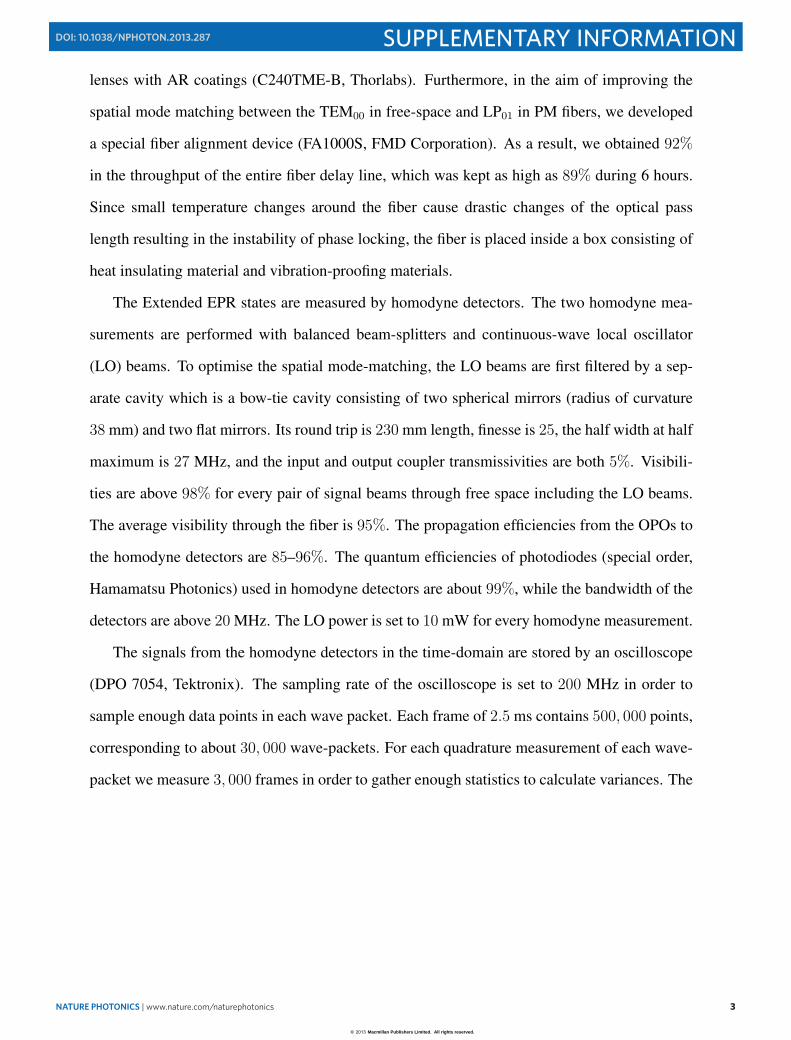
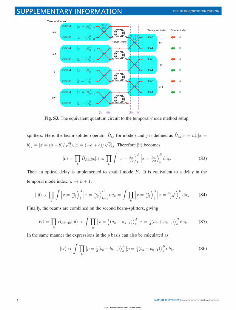
An equivalent linear optics network to our experimental setup is represented in Fig. S3. In this

section we derive the expressions of the extended EPR state by following this circuit with both

4




Beam splitter

Fiber delay line

Optical parametric oscillator

Homodyne detection

Squeezed mode

EPR mode

Graph mode

Entanglement strengths

+1

- 1/2

+1/2

Fig. S2. Legend for animation of experimental setup.

Schrodinger and Heisenberg evolutions. In the Schrodinger picture, we assume the ideal case

where the resource squeezing levels are infinite. On the other hand we can calculate experimen-

tally realistic expressions in the Heisenberg picture.

S2.1.1 Schrodinger Picture in the Ideal Case

Here we utilise infinite squeezing for simplicity. As per the following calculations with Schro-

dinger evolution, the output state is a simultaneous eigenstate of nullifiers. First, there are

position and momentum eigenstates with zero eigenvalue in each temporal location k. Each row

in Fig. S3 shows the spatial mode index which the temporal-mode method would correspond

to. The ket vector |i〉 in step (i) is represented as

|i〉 =∏k

|x = 0〉Ak |p = 0〉Bk ∝∏k

∫|x = 0〉Ak |x = ak〉Bk dak. (S2)

Note that we omit the interval of an integral in this text when the integral interval is from −∞

to ∞. Second, x and p eigenstates in each temporal location are combined by the first beam-

5




OPO-A

HD-B A

B

A

B

A

B

HD-B

HD-A

HD-A

HD-A

HD-B

OPO-B

OPO-B

OPO-B

OPO-B

OPO-A

OPO-A

OPO-A

Temporal index

Temporal index Spatial index

k+1

k+1

k

k

k-1

k-2

k-1

50:50BS

50:50BS

Fiber Delay

(iii) (iv)(i) (ii)

Fig. S3. The equivalent quantum circuit to the temporal-mode method setup.

splitters. Here, the beam-splitter operator Bi,j for mode i and j is defined as Bi,j|x = a〉i|x =

b〉j = |x = (a+ b)/√2〉i|x = (−a+ b)/

√2〉j . Therefore |ii〉 becomes

|ii〉 =∏k

BAk,Bk|i〉 ∝∏k

∫ ∣∣∣x = ak√2

⟩A

k

∣∣∣x = ak√2

⟩B

kdak. (S3)

Then an optical delay is implemented to spatial mode B. It is equivalent to a delay in the

temporal mode index: k → k + 1,

|iii〉 ∝∏k

∫ ∣∣∣x = ak√2

⟩A

k

∣∣∣x = ak√2

⟩B

k+1dak =

∫ ∏k

∣∣∣x = ak√2

⟩A

k

∣∣∣x = ak−1√2

⟩B

kdak. (S4)

Finally, the beams are combined on the second beam-splitters, giving

|iv〉 =∏k

BBk,Ak|iii〉 ∝∫ ∏

k

∣∣x = 12(ak − ak−1)

⟩Ak

∣∣x = 12(ak + ak−1)

⟩Bkdak. (S5)

In the same manner the expressions in the p basis can also be calculated as

|iv〉 ∝∫ ∏

k

∣∣p = 12(bk + bk−1)

⟩Ak

∣∣p = 12(bk − bk−1)

⟩Bkdbk. (S6)

6




Since the output extended EPR state |XEPR〉 is equal to |iv〉, the nullifiers obviously become

zero as

(xAk + xB

k + xAk+1 − xB

k+1

)|XEPR〉 = 0, (S7)

(pAk + pBk − pAk+1 + pBk+1

)|XEPR〉 = 0. (S8)

S2.1.2 Heisenberg Evolution with Finite Squeezing

In the Heisenberg evolution, the variances of nullifiers in the case of finite resource squeezing

levels can be calculated. The complex amplitudes aA(i)k and a

B(i)k of the initial state in step (i)

are represented as

(i) aA(i)k = e−rAx

A(0)k + i erA p

A(0)k , a

B(i)k = erB x

B(0)k + i e−rB p

B(0)k , (S9)

where e−rAxA(0)k and e−rB p

B(0)k are the squeezed quadratures of the k-th squeezed state in the

spatial location A and B, respectively. So we have

⟨xA(0)k

⟩=

⟨pA(0)k

⟩=

⟨xB(0)k

⟩=

⟨pB(0)k

⟩= 0, (S10)

⟨(xA(0)k

)2⟩=

⟨(pA(0)k

)2⟩=

⟨(xB(0)k

)2⟩=

⟨(pB(0)k

)2⟩=

1

4. (S11)

After combining the terms through the action of a beam-splitter they become

(ii)

(aA(ii)k

aB(ii)k

)= B†

Ak,Bk

(aA(i)k

aB(i)k

)BAk,Bk =

1√2

(1 1−1 1

)(aA(i)k

aB(i)k

). (S12)

Subsequently, the of optical delay for mode B is represented as

(iii) aA(iii)k = a

A(ii)k , a

B(iii)k = a

B(ii)k−1 . (S13)

Finally, by combining them on the last beam-splitter the final complex amplitudes of the output

state are given:

(iv)

(aB(iv)k

aA(iv)k

)= B†

Bk,Ak

(aB(iii)k

aA(iii)k

)BBk,Ak =

1√2

(1 1−1 1

)(aB(iii)k

aA(iii)k

)

=1

2

(aA(i)k + a

B(i)k − a

A(i)k−1 + a

B(i)k−1

aA(i)k + a

B(i)k + a

A(i)k−1 − a

B(i)k−1

), (S14)

7




Since aAk = aA(iv)k and aBk = a

B(iv)k , the ideal nullifiers of the extended EPR state are expressed

as

xAk + xB

k + xAk+1 − xB

k+1 = 2 e−rAxA(0)k , (S15)

pAk + pBk − pAk+1 + pBk+1 = 2 e−rB pB(0)k . (S16)

Therefore, we can calculate the nullifier variances which determine the theoretical value of the

inseparable condition as shown in the main text [Eq. (3)],

⟨(xAk + xB

k + xAk+1 − xB

k+1

)2⟩= e−2rA <

1

2, (S17)

and⟨(pAk + pBk − pAk+1 + pBk+1

)2⟩= e−2rB <

1

2. (S18)

This shows that the sufficient condition for inseparability is satisfied when −3 dB resource

squeezing in each OPO is available.

S2.2 Inseparability Criteria for Extended EPR States

Here, we discuss sufficient conditions of entanglement for the extended EPR states, based on

the van Loock-Furusawa inseparability criteria1. We consider all of the cases where an approx-

imate extended EPR state is separable into two subsystems S1 and S2. A necessary condition

of separability is obtained as an inequality for each case. If all of the separable cases are de-

nied by not satisfying the inequalities, the state is proved to be in an entangled state with full

inseparability.

First, we consider the combinations of four nodes {Ak, Bk, Ak+1, Bk+1} distributed into the

two subsystems. When all of the four are not distributed into either subsystem, the possible

cases are as below. Here we abbreviate the nullifiers as Xk ≡ xAk + xB

k + xAk+1 − xB

k+1 and

Pk ≡ pAk + pBk − pAk+1 + pBk+1.

• Case: {Ak} ⊂ S1, {Bk, Ak+1, Bk+1} ⊂ S2.

8




The addition of nullifier variances always satisfies the following inequality:

⟨X2

k

⟩+⟨P 2k

⟩≥ 1

2(|1|+ |1− 1− 1|) = 1. (S19)

• Case: {Bk} ⊂ S1, {Ak, Bk, Bk+1} ⊂ S2.


⟨X2

k

⟩+⟨P 2k

⟩≥ 1

2(|1|+ |1− 1− 1|) = 1. (S20)

• Case: {Ak+1} ⊂ S1, {Ak, Bk, Bk+1} ⊂ S2.


⟨X2

k

⟩+⟨P 2k

⟩≥ 1

2(| − 1|+ |1 + 1− 1|) = 1. (S21)

• Case: {Bk+1} ⊂ S1, {Ak, Bk, Ak+1} ⊂ S2.


⟨X2

k

⟩+⟨P 2k

⟩≥ 1

2(| − 1|+ |1 + 1− 1|) = 1. (S22)

• Case: {Ak, Bk} ⊂ S1, {Ak+1, Bk+1} ⊂ S2.


⟨X2

k

⟩+⟨P 2k

⟩≥ 1

2(|1 + 1|+ | − 1− 1|) = 2. (S23)

• Case: {Ak, Ak+1} ⊂ S1, {Bk, Bk+1} ⊂ S2.


⟨X2

k

⟩+⟨P 2k+1

⟩≥ 1

2(|1|+ | − 1|) = 1. (S24)

9




• Case: {Ak, Bk+1} ⊂ S1, {Bk, Ak+1} ⊂ S2.


⟨X2

k

⟩+⟨P 2k+1

⟩≥ 1

2(| − 1|+ |1|) = 1. (S25)

Therefore, when the inequalities⟨X2

k

⟩+

⟨P 2k

⟩< 1 and

⟨X2

k

⟩+

⟨P 2k+1

⟩< 1 are satisfied,

any of the seven inequalities (S19)–(S25) is not satisfied, which means that the four nodes

{Ak, Bk, Ak+1, Bk+1} are not separable into two subsystem S1 and S2.

Then, we apply the same discussion for all temporal indices k. When the inequalities⟨X2

k

⟩+

⟨P 2k

⟩< 1 and

⟨X2

k

⟩+

⟨P 2k+1

⟩< 1 are satisfied for all k, any partitioning of the

whole system is denied, which means that all nodes are entangled. We may take a more severe

but simpler sufficient condition for entanglement as

⟨X2

k

⟩<

1

2and

⟨P 2k

⟩<

1

2, (S26)

for all k, which is shown in Eq. (3) of the main text.

S2.3 Graph Correspondence

In this section, we discuss the intuitive representation of the extended EPR state in terms of

the graphical calculus for Gaussian pure states2. Every N -mode zero-mean Gaussian pure state

can be uniquely represented by an undirected complex-weighted graph Z, whose imaginary part

(i.e., that of the adjacency matrix for the graph) is positive definite. (In what follows, we make

no distinction between a graph and its adjacency matrix.) The graph Z shows up directly in the

position-space wavefunction for the corresponding state |ψZ〉 (with � = 12):

x〈s|ψZ〉 = ψZ(s) ∝ exp[isTZs

]. (S27)

10




Any Gaussian pure state |ψZ〉 satisfies a set of exact nullifier relations based on its associated

complex matrix Z (ref. 2):

(p− Zx) |ψZ〉 = 0, (S28)

where p and x are column vectors of momentum and position operators, respectively. The

special case of the N -mode ground state (Zground = iI) is easy to verify by noting that the vector

of nullifiers in that case is just the vector of annihilation operators.

The extended EPR state is exactly the state originally proposed by Menicucci in ref. 3. In

that proposal, it was shown that such a state is locally equivalent (up to phase shifts on half the

modes) to a CV cluster state, which is a universal resource for measurement-based quantum

computing with continuous variables4,5. Since measurement-based quantum computation re-

quires the ability to do homodyne detection of any (rotated) quadrature, plus photon counting5,

the phase shifts required to transform the generated state (the extended EPR state) into a CV

cluster state do not need to be physically performed on the state after generation. Instead, one

can account for them entirely just by updating the measurement-based protocol to be imple-

mented (i.e., redefine quadratures x → p and p → −x on the appropriate modes)3. Because of

this equivalence, the original proposal3 used a simplified graphical calculus that blurred the dis-

tinction between the extended EPR state and corresponding CV cluster state since the two were,

for quantum computational purposes, effectively the same resource. The distinction between

these states turns out to make a huge difference, however, when one tries to experimentally

characterize the generated state. In this case, it is much easier to work with the mathematics of

the extended EPR state.

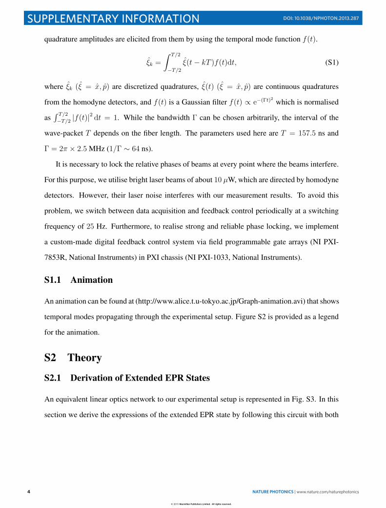
For clarity and completeness, here we present the full complex-weighted graph ZE (ref. 2)

corresponding to the extended EPR state originally proposed in ref. 3 and reported on in this

work:

11




ic

is/2

–is/2

is/2

is/2

–is/2

–is/2ZE = … …

ic

k+1 k k–1 temporal mode index

B

A

spatialmodeindex

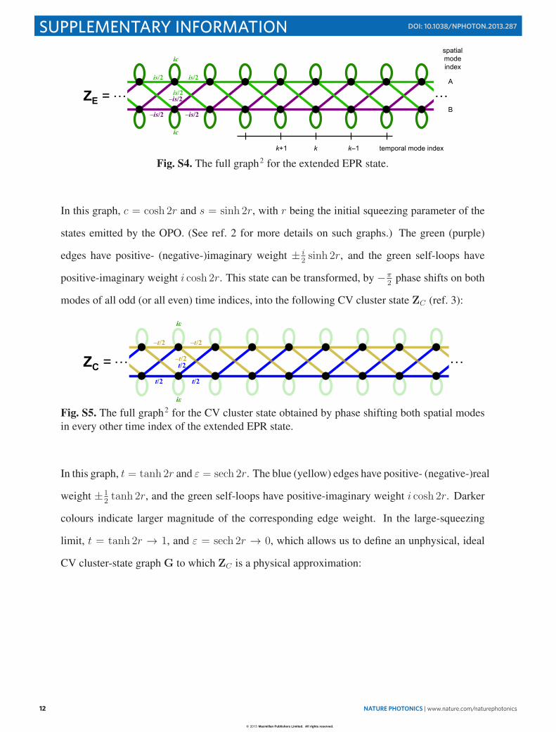
Fig. S4. The full graph2 for the extended EPR state.

In this graph, c = cosh 2r and s = sinh 2r, with r being the initial squeezing parameter of the

states emitted by the OPO. (See ref. 2 for more details on such graphs.) The green (purple)

edges have positive- (negative-)imaginary weight ± i2sinh 2r, and the green self-loops have

positive-imaginary weight i cosh 2r. This state can be transformed, by −π2

phase shifts on both

modes of all odd (or all even) time indices, into the following CV cluster state ZC (ref. 3):

i!

–t/2

t/2

i!

–t/2

–t/2

t/2

t/2ZC = … …

Fig. S5. The full graph2 for the CV cluster state obtained by phase shifting both spatial modesin every other time index of the extended EPR state.

In this graph, t = tanh 2r and ε = sech 2r. The blue (yellow) edges have positive- (negative-)real

weight ±12tanh 2r, and the green self-loops have positive-imaginary weight i cosh 2r. Darker

colours indicate larger magnitude of the corresponding edge weight. In the large-squeezing

limit, t = tanh 2r → 1, and ε = sech 2r → 0, which allows us to define an unphysical, ideal

CV cluster-state graph G to which ZC is a physical approximation:

12




–1/2

1/2

–1/2

–1/2

1/2

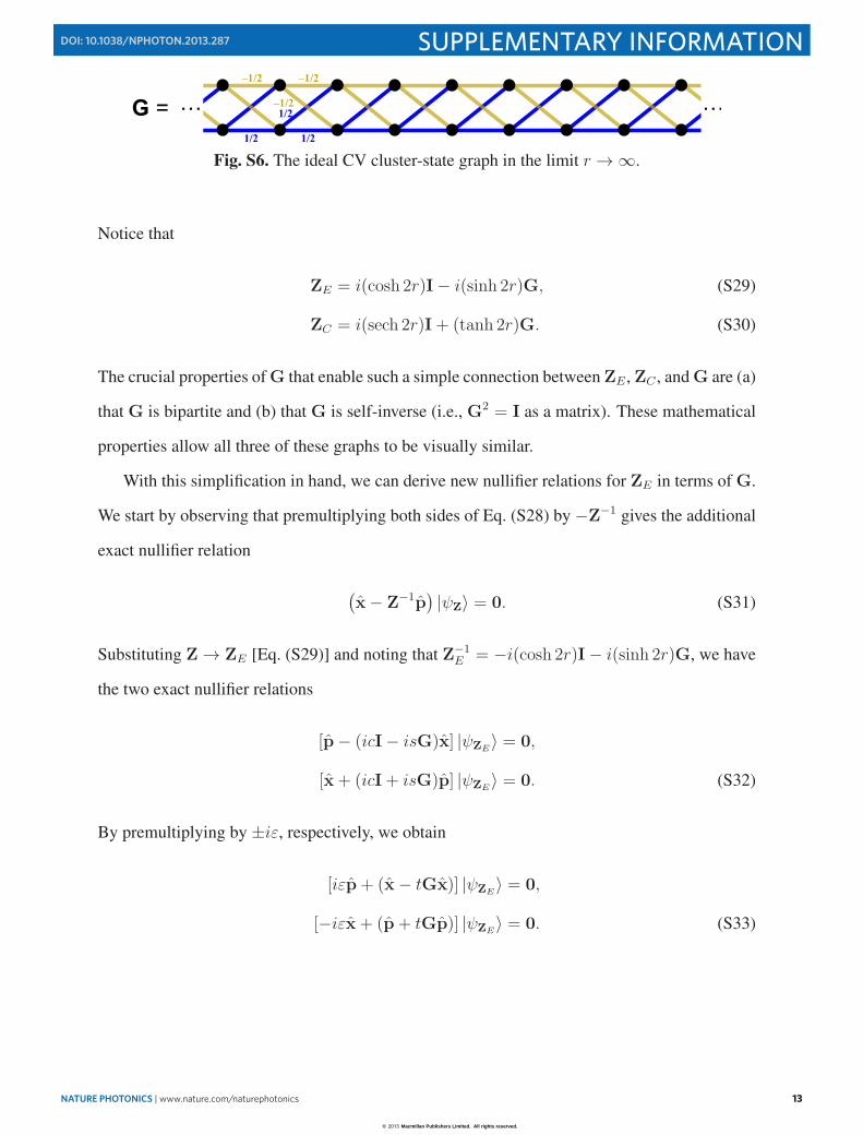
1/2G = … …

Fig. S6. The ideal CV cluster-state graph in the limit r → ∞.

Notice that

ZE = i(cosh 2r)I− i(sinh 2r)G, (S29)

ZC = i(sech 2r)I+ (tanh 2r)G. (S30)

The crucial properties of G that enable such a simple connection between ZE , ZC , and G are (a)

that G is bipartite and (b) that G is self-inverse (i.e., G2 = I as a matrix). These mathematical

properties allow all three of these graphs to be visually similar.

With this simplification in hand, we can derive new nullifier relations for ZE in terms of G.

We start by observing that premultiplying both sides of Eq. (S28) by −Z−1 gives the additional

exact nullifier relation

(x− Z−1p

)|ψZ〉 = 0. (S31)

Substituting Z → ZE [Eq. (S29)] and noting that Z−1E = −i(cosh 2r)I− i(sinh 2r)G, we have

the two exact nullifier relations

[p− (icI− isG)x] |ψZE〉 = 0,

[x+ (icI+ isG)p] |ψZE〉 = 0. (S32)

By premultiplying by ±iε, respectively, we obtain

[iεp+ (x− tGx)] |ψZE〉 = 0,

[−iεx+ (p+ tGp)] |ψZE〉 = 0. (S33)

13




In the large-squeezing limit (r → ∞), ε → 0 and t → 1, and we have the following approximate

nullifiers for the extended EPR state:

(x−Gx) |ψZE〉 r→∞−−−→ 0,

(p+Gp) |ψZE〉 r→∞−−−→ 0. (S34)

This is the state we have created. For completeness, however, we can compare these to the exact

and approximate nullifiers for the associated CV cluster state |ψZC〉 obtained by phase shifting

particular nodes as described above (either actively or by simply redefining quadratures used for

the measurements). Substituting Z → ZC [Eq. (S30)] and noting that Z−1C = −i(sech 2r)I +

(tanh 2r)G, the exact nullifiers are

(−iεx+ p− tGx) |ψZC〉 = 0,

(iεp+ x− tGp) |ψZC〉 = 0, (S35)

which, in the large-squeezing limit, reduce to the following approximate nullifiers:

(p−Gx) |ψZC〉 r→∞−−−→ 0,

(x−Gp) |ψZC〉 r→∞−−−→ 0. (S36)

Once again, these simple and symmetric expressions in terms of G are unusual and only possi-

ble because G is bipartite and self-inverse2.

S2.4 Equivalence to Sequential Teleportation-based Quantum Computa-tion Circuit

In reference 3, Menicucci proposed that by erasing half of the state (one rail), the cluster states

can be used as resources for measurement-based quantum computation (MBQC). However,

erasing half of the state is a wasteful process and it is experimentally hard to perform the nec-

essary feedforwards to future and past modes in the time axis. Here, we show that the extended

14




EPR state is a resource for MBQC, and that we can fully utilise every degree of freedom without

erasing half of the state. We devise a much more efficient method of using this resource state

for quantum computation than the method originally proposed in ref. 3, in terms of its use of the

available squeezing resources. Specifically, arbitrary Gaussian operation may be implemented

by only 4 measurements, which is more efficient than the 8 measurements necessary with the

original method6. Furthermore, we show that non-Gaussian operations may be performed on

the extended EPR state by introducing non-Gaussian measurements, leading to one-mode uni-

versal MBQC.

S2.4.1 Gaussian Operation

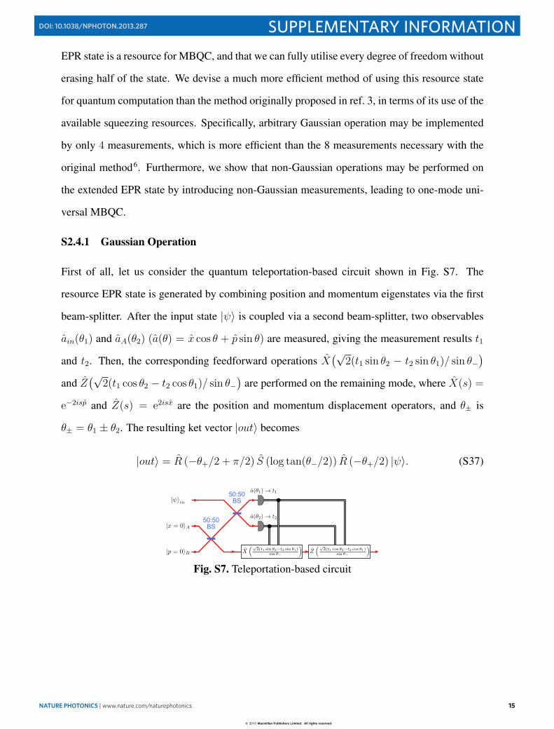
First of all, let us consider the quantum teleportation-based circuit shown in Fig. S7. The

resource EPR state is generated by combining position and momentum eigenstates via the first

beam-splitter. After the input state |ψ〉 is coupled via a second beam-splitter, two observables

ain(θ1) and aA(θ2) (a(θ) = x cos θ + p sin θ) are measured, giving the measurement results t1

and t2. Then, the corresponding feedforward operations X(√

2(t1 sin θ2 − t2 sin θ1)/ sin θ−)

and Z(√

2(t1 cos θ2 − t2 cos θ1)/ sin θ−)

are performed on the remaining mode, where X(s) =

e−2isp and Z(s) = e2isx are the position and momentum displacement operators, and θ± is

θ± = θ1 ± θ2. The resulting ket vector |out〉 becomes

|out〉 = R (−θ+/2 + π/2) S (log tan(θ−/2)) R (−θ+/2) |ψ〉. (S37)

50:50BS

50:50BS

Fig. S7. Teleportation-based circuit

15




50:50BS

50:50BS

50:50BS

50:50BS

50:50BS

50:50BS

Extended EPR state

Extended EPR state Input Coupling

Input Couplinga b

c-1/2 -1/√2

1/√2 1/2

mode index

A0

A0

B1

B1

A1

A1

B2

B2

A2

A2

B3

B3

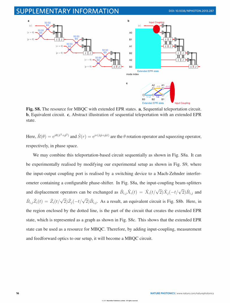
Fig. S8. The resource for MBQC with extended EPR states. a, Sequential teleportation circuit.b, Equivalent circuit. c, Abstract illustration of sequential teleportation with an extended EPRstate.

Here, R(θ) = eiθ(x2+p2) and S(r) = eir(xp+px) are the θ rotation operator and squeezing operator,

respectively, in phase space.

We may combine this teleportation-based circuit sequentially as shown in Fig. S8a. It can

be experimentally realised by modifying our experimental setup as shown in Fig. S9, where

the input-output coupling port is realised by a switching device to a Mach-Zehnder interfer-

ometer containing a configurable phase-shifter. In Fig. S8a, the input-coupling beam-splitters

and displacement operators can be exchanged as Bi,jXi(t) = Xi(t/√2)Xj(−t/

√2)Bi,j and

Bi,jZi(t) = Zi(t/√2)Zj(−t/

√2)Bi,j . As a result, an equivalent circuit is Fig. S8b. Here, in

the region enclosed by the dotted line, is the part of the circuit that creates the extended EPR

state, which is represented as a graph as shown in Fig. S8c. This shows that the extended EPR

state can be used as a resource for MBQC. Therefore, by adding input-coupling, measurement

and feedforward optics to our setup, it will become a MBQC circuit.

16




50:50BS

50:50BS

LO

Fiber Delay

Input Port Output Port

OPOs

HD-A

HD-B

LO

SW

Disp.

a

Fiber Delay

Input Port Output PortSW

Disp.

b

Fiber Delay

Input Port Output Port

Output State

SW

Disp.

c

d

Input Coupling(Bell Measurement)

Feedforward(Displacement)

...

=

Bell Measurement

...

...

Input State

Sequential EPR states

Feedforward(Displacement)

SW

EOM(θ=0)

=SW

EOM(θ=π)

50:50BS

50:50BS

Fig. S9. Experimental setup (left) and abstract illustration (right) for MBQC with extendedEPR states. a, Input coupling. b, Sequential MBQC. c, Output. d, Switching (SW) device withMach-Zehnder interferometer including electro optical modulator (EOM).

S2.4.2 Non-Gaussian Operation

Non-Gaussian operations may also be implemented by using the teleportation-based circuit

shown in Fig. S10. It is derived in the following way. The ket vector after input coupling is

represented as

Bin,A|ψ〉in ⊗(BA,B|x = 0〉A|p = 0〉B

)

∝∫

dtx|x = tx〉inXA(tx)XB(√2 tx)⊗

(∫dξ ψ(ξ)

∣∣x = −√2 ξ

⟩A

∣∣x = −ξ⟩B

). (S38)

17




50:50BS

50:50BS

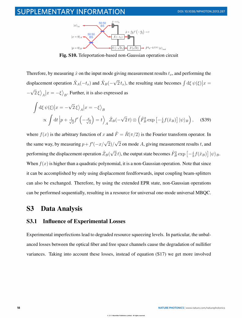
Fig. S10. Teleportation-based non-Gaussian operation circuit

Therefore, by measuring x on the input mode giving measurement results tx, and performing the

displacement operation XA(−tx) and XB(−√2 tx), the resulting state becomes

∫dξ ψ(ξ)

∣∣x =

−√2 ξ

⟩A

∣∣x = −ξ⟩B

. Further, it is also expressed as

∫dξ ψ(ξ)

∣∣x = −√2 ξ

⟩A

∣∣x = −ξ⟩B

∝∫

dt∣∣∣p+ 1√

2f ′(− x√

2

)= t

⟩AZB(−

√2 t)⊗

(F 2B exp

[− i

�f(xB)]|ψ〉B

), (S39)

where f(x) is the arbitrary function of x and F = R(π/2) is the Fourier transform operator. In

the same way, by measuring p+f ′(−x/√2)/

√2 on mode A, giving measurement results t, and

performing the displacement operation ZB(√2 t), the output state becomes F 2

B exp[− i

�f(xB)]|ψ〉B.

When f(x) is higher than a quadratic polynomial, it is a non-Gaussian operation. Note that since

it can be accomplished by only using displacement feedforwards, input coupling beam-splitters

can also be exchanged. Therefore, by using the extended EPR state, non-Gaussian operations

can be performed sequentially, resulting in a resource for universal one-mode universal MBQC.

S3 Data Analysis

S3.1 Influence of Experimental Losses

Experimental imperfections lead to degraded resource squeezing levels. In particular, the unbal-

anced losses between the optical fiber and free space channels cause the degradation of nullifier

variances. Taking into account these losses, instead of equation (S17) we get more involved

18




theoretical values given by:

⟨X2

k

⟩= 1

4

(ηA + ηAF

)2(SqA − 1) + 1

4

(ηB − ηBF

)2(ASqB − 1) + 1,⟨

P 2k

⟩= 1

4

(ηB + ηBF

)2(SqB − 1) + 1

4

(ηA − ηAF

)2(ASqA − 1) + 1,

(S40)

where SqΓ and ASqΓ are squeezing and anti-squeezing terms for beam Γ(= A,B), and η2Γ and

(ηFΓ )2 are the effective efficiencies of squeezing levels for beam Γ through the free space and

optical fiber channels, respectively. To be more precise, η is given by: (quantum efficiency at

homodyne detector) × (influence of intracavity loss T/(T + L)) × (visibility between probe

and LO beams)2 × (propagation efficiency), where T is the transmittance of the output coupler

and L is the intracavity loss in the OPO. In the experiment, these efficiencies are η2A = 88.2%,

η2B = 89.9%, (ηFA)2 = 73.7% and (ηFB)

2 = 75.3%. Squeezing levels are calculated as

Sq =

∫|f(ω)|2 R−(ω)dω, ASq =

∫|f(ω)|2 R+(ω)dω, (S41)

R±(ω) = 1± (1− η(ω))4x

(1∓ x)2 + (ω/γ)2, (S42)

where f(ω) is the Fourier transformation of mode function f(t), η(ω) is the ratio of electrical

noise to shot noise at angular frequency ω, x is the pump parameter which is related to the

classical parametric amplification gain G as G = (1 − x)−2, and γ is the angular frequency

half width at half maximum of the OPO. By substituting in these experimental values, we get⟨X2

k

⟩= −5.13 dB and

⟨P 2k

⟩= −5.33 dB. They agree well with experimental results.

References

1. van Loock, P., & Furusawa, A. Detecting genuine multipartite continuous-variable entan-

glement. Phys. Rev. A 67, 052315 (2003).

2. Menicucci, N. C. Flammia, S. T. & van Loock, P. “Graphical calculus for Gaussian pure

states,” Phys. Rev. A 83, 042335 (2011).

19




3. Menicucci, N. C. Temporal-mode continuous-variable cluster states using linear optics.

Phys. Rev. A 83, 062314 (2011).

4. Menicucci, N. C. et al. Universal Quantum Computation with Continuous-Variable Cluster

States. Phys. Rev. Lett. 97, 110501 (2006).

5. Gu, M., Weedbrook, C., Menicucci, N. C. Ralph, T. C. & van Loock, P. “Quantum Com-

puting with Continuous-Variable Clusters,” Phys. Rev. A 79, 062318 (2009).

6. Alexander, R. et al. Optimising the temporal mode scheme for single qumode Gaussian

operations. in preparation.

Acknowledgments: N.C.M. is grateful to R. Alexander, and P. van Loock for helpful discus-

sions.

20


Supplementary Information for Ultra-Large-Scale … · Supplementary Information for...

Documents

Transcript of Supplementary Information for Ultra-Large-Scale … · Supplementary Information for...