1

Supplementary Information Appendix for:

Chromatin conformation governs T cell receptor Jβ gene segment usage

Wilfred Ndifon*, Hilah Gal*, Eric Shifrut, Rina Aharoni, Nissan Yissachar, Nir Waysbort,

Shlomit Reich-Zeliger, Ruth Arnon, Nir Friedman

*Joint first authors

This file includes:

Supplementary methods

Supplementary text

Figures S1 - S17

Tables S1 – S9

2

Supplementary methods

1. Library construction and sequencing. We extracted total RNA from splenic T cells of

C57BL/6 mice using RNeasy Mini Kit (Qiagen). The RNA was reverse transcribed using

SuperScriptTM

II reverse transcriptase (Invitrogen), and a TCR Cβ-specific primer linked to the

3'-end Illumina sequencing adapter (Cβ-3’adp). The resulting cDNA was used as template for

high fidelity PCR amplification (Phusion, Finnzymes) using the Cβ-3’adp primer and 23 Vβ-

specific primers, each of which was anchored to a restriction site sequence for the ACUI

restriction enzyme (NEB). The Vβ primers were divided into 5 groups that where PCR amplified

in parallel, in order to minimize the potential for cross hybridization. The PCR reactions (18

cycles) were performed in triplicates, and PCR products were then pooled and cleaned using

QIAquick PCR purification kit (Qiagen), followed by enzymatic digestion of 0.5-1.5 μg of

cleaned PCR product, in accordance with ACUI protocol (NEB). The ACUI enzyme was used to

cleave the + (-) cDNA strand 16 bp (14 bp) downstream of its binding site, such that sequencing

starts closer to the V-D junction region. This allows for good coverage of CDR3 with a single

Illumina read. ACUI cleavage produces a 2 bp overhang that is used for ligation of the Illumina

5’ adapter, which was linked to a 3 bp barcode sequence in its 3’ end. Overnight ligation was

performed using the T4 ligase (Fermentas) at 16°c in accordance with the manufacturer’s

protocol. A second round of PCR amplification was performed (24 cycles), using primers for the

5’ and 3’ Illumina adapters. Final PCR products were run on a 2% agarose gel and purified using

the Wizard SV Gel and PCR clean-up System (Promega). Final library concentrations were

measured using the nanodrop spectrophotometer. The libraries were sequenced using Genome

Analyzer II (Illumina).

2. Pre-processing of sequence reads and Vβ/Jβ gene assignment. We filtered out reads

containing bases with Q-value ≤20, and then separated the remaining reads according to their

barcodes. Then, we aligned the reads to each of the germline (1) Vβ/Jβ gene segments using the

Smith-Waterman algorithm (2). Each read was assigned its best-aligning Vβ/Jβ if the number of

matching nucleotides (alignment length) was above a threshold, which we defined in the

following way: We randomly sampled 3×105 of the analyzed reads, and randomly permuted the

positions of nucleotides found in each of these reads. We then determined alignment lengths for

the best Vβ and Jβ matches for each permuted read (Fig. S13), and defined a threshold as the

alignment length above which only 1% of the randomly permuted reads are matched. This

procedure gave us the following threshold alignment lengths: For datasets M1-M4 and M7-M8

(40 nt long reads): 11 nt for Vβ, 9 nt for Jβ. For dataset M5 (80 nt long reads): 12 nt for Vβ, 11 nt

for Jβ.

3. Correction of nucleotide misincorporation errors. We clustered reads assigned the same Vβ

and Jβ genes to correct up to r nucleotide misincorporation errors (r=2 for 40 nt reads, and r=3

for 80 nt reads) that occurred, primarily, during high-throughput sequencing. The following

clustering algorithm was used: (i) the read with the greatest number of identical copies was

chosen to seed a new cluster, and (ii) other unclustered reads that had an edit distance of ≤r from

3

the cluster seed were added to the new cluster. Steps (i) and (ii) were repeated until all reads

were clustered.

4. Characterization of sequence clusters. We assigned for each cluster a nucleotide sequence,

and its Vβ and Jβ genes, as those of the cluster seed. For some clusters we can also assign a Dβ

gene by aligning the junction region (Fig. S1c) to the two germline (1) Dβ gene segments.

Because of the high similarity between the two germline Dβ genes we require a perfect match of

length > 6 nt. Next, we used the alignment of the cluster sequences to the corresponding

germline Vβ/Jβ sequences to computationally reconstruct the entire recombined Vβ/Dβ/Jβ

sequence (Fig. S1c). This reconstruction also provides us with the correct reading frame for each

sequence. The reconstructed sequences were then translated to generate the corresponding

amino-acid sequences. Sequences containing a stop codon (including Vβ17+ sequences for which

a stop codon is present in the germline sequence) (1,3,4), were designated as “unselected”, and

the rest as “selected”. We also calculated the number of cleavage errors found in each cluster

sequence, as the absolute difference between the position where its Vβ gene was enzymatically

cleaved during library preparation and the consensus (or median) cleavage position for all cluster

sequences that carry the same Vβ.

5. Correction of sequencing bias. Sequencing bias, defined here as the deviation of a particular

cluster sequence’s relative frequency measured in a given library from its actual relative

frequency in the same library, results mainly from our use of different Vβ-specific primers

during PCR. We corrected this bias by first applying a new, bottom-up probabilistic method that

we developed (see section 9 below). We applied this method to both measured and actual

frequencies of cloned TCRs found in different control plasmids libraries that we constructed and

sequenced (section 9). These 79 plasmids each contain a cloned TCRB sequence, representing all

23 Vβ segments. This application yielded estimates for the bias associated with individual Vβ

primers (Table S9), allowing us to correct sequencing bias by normalizing the measured

frequency for each cluster sequence by the bias for its primer. To increase the signal-to-noise

ratio of our data when calculating repertoire characteristics, we used cluster sequences with ≤2

cleavage errors (see above) and bias-corrected cluster sizes of ≥5. These cluster sequences were

designated as clonotypes.

6. Biophysical model for gene rearrangement frequency. We adapted a previously published

model (5) to calculate gene frequencies. The biophysical model gives the theoretical frequency

of the ith Jβ gene as: P(Jβi)=K[α1-3/2

exp(-2α1-2

)+α2-3/2

exp(-2α2-2

)], where αj=(dj/b)(1-dj/c), j=1,2.

di,j (in bp) is the genomic distance between the start position of the 12-RSS of Jβi and the start

position of the 23-RSS of Dβj (Table S4), K is a normalization constant, and both b (in nm) and c

(in bp) are free parameters. We fit the model to our measured Dβ-Jβ frequencies (Table S3),

normalized so that they sum to 1, by minimizing the sum of squared differences between the

empirical relative frequencies and the corresponding theoretical relative frequencies predicted by

the model, first by means of simulated annealing (6), and then by means of gradient descent. See

Supplementary text, section 2, for additional information about the model fit.

4

7. Statistical analysis. We did only nonparametric tests for significance in order to limit the

dependence of results on distributional assumptions. We tested for significance of the similarity

(quantified as the squared Pearson correlation, R2) between two vectors of relative frequencies by

randomly permuting the entries of one vector, and then calculating the R2 value between both

vectors. This procedure was repeated 100 times, unless indicated otherwise, and the maximum of

either 1/100 or the fraction of the permutation-derived R2

values that exceeded the original R2

value was reported as the p-value for the test. In addition, we tested for significance of the

difference between two vectors of average relative frequencies using the two-sided Wilcoxon

signed rank test. This test involves the reasonable assumption that the vector difference comes

from a continuous, symmetric distribution.

8. Sequence sharing analysis. For the analysis described in Figure 4a, we assigned an amino-

acid sequence to all selected clonotypes in datasets M1-M5. Clonotypes of different nucleotide

sequences that have the same amino-acid sequence were pooled together. We then sampled

randomly 15,000 unique amino-acid sequences from each dataset, where the chance of selection

is proportional to the number of times each amino-acid sequence appears in the dataset. This

allows for analysis of sharing between datasets of different sizes based on an equal number of

unique sequences down-sampled from the total sequences. This procedure provides direct

comparison of data and model, which is based on the a-priori frequency of generating unique

sequences (see Supplementary text, section 3). For the analysis described in Figure 4b, we

similarly sampled 2,000 unique sequences out of unselected clonotypes (as these sequences

include a stop codon in their reading frame, it is included as an extra letter in the alphabet

describing unselected amino-acid sequences).

9. A method for correcting PCR induced sequencing bias

Here we develop a mechanistically motivated, bottom-up method for correcting sequencing bias

introduced by PCR amplification during library construction. These biases occur in our TCR-seq

protocol, as well as in other such protocols, due to the use of a set of primers that introduce

biases in the efficiencies of cDNA amplification. We develop the method in two steps. Firstly,

using techniques drawn from the fields of combinatorics (7) and stochastic dynamics (8), we

derive an equation for the probability distribution of a clonotype’s copy number conditioned on

parameters of the PCR reaction. This distribution turns out to be a negative binomial. The

negative binomial distribution has previously proved very useful for the analysis of RNA-seq

data, especially because of its ability to account for the over-dispersion often observed in such

data. These previous applications were sometimes justified phenomenologically by appealing to

the fact that the negative binomial distribution arises if each copy number is drawn from a

Poisson distribution whose mean is a gamma-distributed random variable. However, the

parameters of the negative binomial distribution were not always given clear biological

interpretations. In contrast, our analytical results provide a less arbitrary rationale for applying

the negative binomial distribution to RNA-seq data, and they also allow us to interpret the

5

distribution’s parameters in terms of parameters of the PCR reaction used in our TCR-seq

method.

In the second step of the development of our method for bias correction, we incorporate the

effect of amplicon subsampling into the derived negative binomial distribution, resulting in a

superposition of this distribution with the binomial distribution. We also derive an approximation

for the resulting distribution that is both accurate and easy to evaluate. We conclude by

discussing how we applied our method to sequencing data.

9.1 PCR amplification: We begin by considering the fate of a particular clonotype (denoted

clonotype i) whose cDNAs are found in a library that is PCR amplified and then sequenced. Let

Ni be the initial copy number of clonotype i (i.e., Ni is the number of cDNA molecules derived

from clonotype i). Also, let Xi,t be a random variable representing the clonotype’s copy number at

the t'th PCR cycle. To simplify the notation, we will drop t from the subscript of Xi,t. During each

PCR cycle, the individual copies of Xi will be replicated with a probability corresponding to the

PCR amplification efficiency. Differences in PCR amplification efficiency occurring between

clonotypes will depend on the PCR primer for each clonotype’s Vβ gene, and possibly other

factors (i.e., GC content and cDNA length). We model the PCR amplification of clonotype i as a

Markov jump process (8), in which there are small discrete increases in Xi occurring at small

time intervals (PCR cycles), and the magnitude of the increase occurring at one time interval

depends directly only on the state of the reaction in the immediately preceding time interval. This

model yields an equation for the probability distribution of Xi conditioned on the PCR

amplification efficiency for clonotype i, the initial (pre-PCR) copy number of clonotype i, and

the number of cycles of the PCR reaction. This model captures very well the average dynamics

of Xi as well as the fluctuations associated with both the discreteness and the smallness of the

cDNA copy number increments. We do not consider any possible mutations that might occur

during the PCR reaction because the mutation rate for a high-fidelity DNA polymerase, such as

the one used here, is very small, especially compared with sequencing error rate, so the

frequency of mutants introduced by PCR will in general be negligible.

Based on the above discussion, the master equation for the dynamics of the probability

distribution of Xi is given by:

','|,','|,11','|, txXtxXpxrtxXtxXpxrtxXtxXp iiiiiiiiiiiiiiit , (S1)

where ','|, txXtxXp iii denotes the conditional probability that clonotype i has xi copies at

time t given that it had xi’ copies at time t’. ir is the probabilistic rate of increase of Xi, which

corresponds to the PCR amplification efficiency for clonotype i. We assume that ir is constant,

which is reasonable for the relatively short duration of the PCR reactions considered here

(empirical evidence indicates that ir will eventually decrease if the PCR reaction lasts long

enough that the dynamics of cDNA copies reaches a plateau phase). The analysis we will

6

perform can be adapted to model PCR reactions in which ir is assumed time-dependent. For ease

of presentation we will abbreviate ','|, txXtxXp iii by txp i , .

We will derive txp i , by using a powerful combinatorial device called the generating

function (7). Specifically, the (probability) generating function for Xi is defined as:

txpstsG ix

x

i

i ,,0

. (S2)

Observe that, by definition,

1,,10

ix

i txptG , isi

x

x

iss xtxpsxtsGi

i

10

1

1,, , and (S3)

1,1,1

0

2

1

2

iisi

x

x

iis

s xxtxpsxxtsGi

i . (S4)

Also, observe that the coefficient of ixs in tsG , is txp i , , hence the name “probability

generating function”.

Multiplying both sides of (S1) by ixs and summing over all possible values of xi gives:

000,,11,

i

i

i

i

i

i

x ii

x

iiix

x

ix it

xtxpxsrtxpxsrtxps , (S5)

which can be simplified to [using (S2) and (S3)]:

tsGssrtsG sit ,1, . (S6)

We eliminate s from the coefficient of tsGs , in (S6) by making the substitutions

yes 11 and tsGty ,, , which leads to:

tyrs

yty

yssrtsGty yiitt ,,1,,

. (S7)

The solution of (S7) is a function try i exp , whose exact functional form is determined by

the initial copy number of clonotype i. Thus, we can express tsG , as:

triesstsG 1, 1 . (S8)

If at time t=0 there are Ni copies of clonotype i, then p(x,0) equals 0 if x Ni and it equals 1

otherwise. Therefore:

0

1 0,10,x

Nx isxpssssG , (S9)

implying that

7

iiiii

NtrNtrNsesetsG

11, . (S10)

The probability distribution of interest, txp i , , is given by the coefficient of ixs in tsG , ,

which we denote by ixs . It can be obtained by expanding tsG , in a power series in s, which

yields (after some algebra):

iiiii

NxtrtrN

ii

i

i eeNx

xtxp

1

1, (S11)

tr

iiiieNNx

,,A , (S12)

where A denotes the negative binomial distribution. Using (S3), (S4) and (S10) we see that the

mean and the variance of Xi are given by

tr

iiieNx and (S13)

trtr

iiiii eeNxx

1

222, (S14)

respectively. It is clear from the above that without PCR amplification (i.e., 0t ) the mean of Xi

is Ni, whereas the variance is 0. However, with PCR amplification the ratio of the variance to the

mean will increase with the duration of PCR, such that the distribution of the copy number of

clonotype i will become over-dispersed. Therefore, (S12) may be useful for the analysis of other

types of RNA-seq data obtained by sequencing PCR-amplified libraries, since it can capture the

over-dispersion often observed in such data, which frequently used distributions such as the

Poisson distribution fail to capture.

It is not very difficult to prove that Eqn. (S11) solves (S1) – e.g., by differentiating the

right-hand side of (S11) and showing that it equals the right-hand side of (S1). Specifically:

1

11

11

,

iiiiii

iiiii

NxtrtrN

ii

itr

iii

NxtrtrN

ii

i

iiit eeNx

xeNxree

Nx

xrNtxp

txpe

eNxrtxprN itr

tr

iiiiii

i

i

,1

,

txpe

Nxr

e

Nxr

e

eNxrrN itr

iii

tr

iii

tr

tr

iiiii

iii

i

,111

txpxrtxpxr iiiiii ,11, ,

as expected.

txpe

Nxrtxpxr itr

iiiiii

i,

1,

8

9.2 Subsampling of PCR amplified cDNAs: After PCR amplification, only a subset of the

obtained cDNAs is subsequently sequenced. This subsampling of the amplicons may occur

because of the need to save a portion of the PCR products for later use, but it is often also

performed prior to Illumina sequencing in order to assure the efficiency and accuracy of the

sequencing reaction. Subsampling helps to ensure that different cDNA clusters will occupy

different spatial locations in the Illumina sequencing instrument, such that the risk for between-

cluster interference in fluorescence signal is minimal. But it can also result in the loss of

clonotypes that have small initial copy numbers and/or relatively small PCR amplification

efficiencies. For example, as the PCR reaction proceeds, the relative frequency of a clonotype

that has a smaller-than-average PCR amplification efficiency would decrease, such that for a

fixed rate of subsampling that clonotype would become increasingly less likely to be sequenced.

This effect can bias significantly statistics of the clonotype repertoire that are based on

comparisons between different subsets of unique clonotypes that differ in their PCR

amplification efficiencies (e.g., because they were amplified using different PCR primers). It is

therefore important to consider the effect that subsampling has on the final sequencing data when

analyzing these data. Note that we do not consider here any amplification bias that might arise

from the PCR reaction occurring inside the sequencer because in this case each newly created

cDNA cluster typically contributes only a single sequence read to the final sequencing data, and

also because all the cDNAs are amplified using universal primers.

We will use the probability generating function to extend the expression for the probability

distribution of Xi derived in the preceding section, in order to account for amplicon subsampling.

Although we can achieve this particular goal in a more direct way, using the probability

generating function will make less complicated the subsequent task of calculating the moments

of Xi. First, we note that the dynamics of the probability distribution of Xi is given by:

,11,, iiiii xpxcxpcxxp , (S15)

where c is the probabilistic rate at which cDNA copies of clonotype i are lost during

subsampling, and 0,ixp is given by (S11). In principle, equals 1 time unit.

The dynamics of the probability generating function corresponding to (S15) is given by:

,~

1,~

sGscsG s . (S16)

Using the same steps we used above, and the fact that 0,~

sG is given by (S10), we obtain

the equations:

fssG 1,~

, and (S17)

iiiii

NtrNtrNfsefsesG

111111

~, (S18)

9

in which, for ease of presentation, we have made the substitution cf exp . Note that f

corresponds to the fraction of sequenced amplicons. txp i , can be obtained from (S18) by using

the following formula for individual terms found in the composition of two generating functions:

k

k

xkxhsgshgs ii

0, (S19)

where the function g is given by (S10), while the function fsh 11 . This leads to the

following expression for the probability distribution of Xi after amplicon subsampling, which

corresponds to a superposition of the negative binomial distribution with the binomial

distribution:

i

iii

iii

Nj

xjx

i

NjtrtrN

i

i ffx

jee

Nj

jtxp 11

1, (S20)

i

i

Nj

i

tr

ii fjxeNNj ,,,, CA . (S21)

In (S21), A and C denote the negative binomial and the binomial distributions, respectively.

An alternative expression for p(xi,t) can be obtained from (S18) by first expanding

iNfs 11 in a Maclaurin series in s, and then finding the coefficient of ix

s in the resulting

expression:

i

ii

ii

ii

N

jNtr

jtrNjNjix

i

fse

seff

j

Nstxp

0 11111, (S22)

ii

iiii

iiii

i

xN

jjxNtrtr

jxtrtrN

i

iijNji

fee

fee

jx

jxNff

j

N,min

0 1

111 (S23)

jxN

eN

fee

fffe

jxjjN

jxN

ii

trN

i

xN

jjxNtrtr

jNjjxtr

ii

iiiiii

iiii

iii

,min

0 1

11

,, (S24)

By using (S3), (S4) and (S18), we obtain the following expressions for the mean and the

variance of Xi, which account for amplicon subsampling:

tr

iiiefNx and (S25)

fefefNxxtrtr

iiiii 21

222

, (S26)

respectively.

In practice, (S24) will be computationally much easier to apply than (S21) because it

requires evaluation of only as many terms as the value of Ni, which is typically much smaller

10

than xi. In fact, it is possible to obtain an accurate estimate for p(xi,t) by evaluating only the first

k<Ni terms in (S24), as individual higher-order terms of the Maclaurin series for iNfs 11

would contain less information about p(xi,t) than individual lower-order terms.

9.3 Application to sequencing data. We applied the method described above to a sequenced

control library containing 79 plasmids, each carrying a known CDR3 sequence, in order to

estimate the bias for each Vβ-specific PCR primer. Samples taken from this control library were

sequenced in three independent experiments. First, one sample was prepared for sequencing

using the same set of 23 Vβ-specific primers as for library M5 (Table S9, column 2). Then, two

other samples were independently prepared using the same Vβ-specific primers as for libraries

M1-M4, M6-M8 (Table S9, column 3). The amounts of different plasmids added to each sample

were varied by serial dilutions of the plasmids in groups of ~13 plasmids each.

Sequence reads (each of length 40 nt) obtained from sequencing the plasmids libraries

were pre-processed and then corrected for nucleotide misincorporation errors, as described in

Methods. The reads were subsequently aligned to the known plasmid CDR3 sequences using the

Smith-Waterman algorithm (2). Each read was grouped together with its best-aligning plasmid,

while allowing an edit distance of ≤2. The observed frequency for each plasmid was defined as

the number of reads grouped with it.

We fit Eqn. (S24) to the plasmids data, where, for each plasmid, x equals its observed

frequency, and N equals its known relative frequency times a constant (whose value we

estimated from the data). The fit was done by maximizing the likelihood of the data, using the

method of simulated annealing (6). For each primer, the fit gave us an estimate for ert, its

amplification factor. Using these amplification factors, the expected frequency of each plasmid is

calculated as N×ert×f [Eq. (S25)]. There is a good correlation (R

2=0.47 and 0.68/0.62 for the two

sets of primers; Fig. S14a) between these calculated expected frequencies and the actually

observed frequencies, especially for the second set of primers. In addition, when the plasmids are

grouped according to their Vβ gene segment, the average of the calculated expected frequencies

of plasmids belonging to the same group is highly correlated with the average observed

frequency for the same group (R2=0.84 – 1; Fig. S14b). These observations support the accuracy

of the estimated amplification efficiencies, especially for the second primer set.

For each library, we calculated the bias for a particular primer as the ratio of the

amplification factor for that primer to the mean amplification factor for all primers (Table S9,

column 4,5). The observed relative frequencies of sequences amplified using primers with bias >

1 (respectively bias < 1) would be greater (respectively less) than the initial relative frequencies.

However, normalizing a sequence’s observed relative frequency by the bias for its primer would

correct this sequencing bias. Therefore, we corrected the sequencing bias found in the

experimental libraries by normalizing the cluster size for each cluster sequence by the bias of the

corresponding Vβ primer. The average bias (geometric mean) is small (<2 for both sets of

primers).

11

To further increase the signal-to-noise ratio of the sequencing data, we mainly used for

further analysis of repertoire characteristics cluster sequences that contain ≤2 cleavage errors

(see Methods for definition) and have a bias-corrected cluster size (i.e., copy number) of ≥5.

These cluster sequences were designated as clonotypes. To check the sensitivity of our results to

this cutoff on copy number, we plotted the Vβ and Jβ frequencies measured in selected (see

Methods for definition) clonotypes, either without a cutoff or with a cutoff of copy number ≥5 or

≥10 (Fig. S15). Jβ frequencies are insensitive to this cutoff (Fig. S15d-f). Some Vβ frequencies

change when the cutoff is increased above 0, but do not change greatly if the cutoff is increased

from 5 to 10 (Fig. S15a-c). The increase in the frequency of Vβ8.2 in dataset M5 that we

measured with a copy number cutoff (Fig. S15a-c) is partly due to the fact that the bias for this

Vβ primer in the primer set used in this particular experiment is very low (Table S9, column 4).

12

Supplementary text

1. Technical controls for our TCR-seq data, and comparisons to published data and to

antibody-based Vβ frequencies

We assessed the effect of the sequencing reaction on measured gene usage by comparing Vβ-Jβ

frequencies obtained from library M2 to corresponding frequencies obtained from a technical

replicate of the same library. We find that both sets of Vβ-Jβ frequencies are highly similar (Fig.

S15), implying that the sequencing reaction does not significantly bias the Vβ-Jβ frequencies.

We also compared the measured Jβ frequencies to published frequencies. We find that our

measured Jβ frequencies are very similar to published murine Jβ frequencies, R2=0.96 (Ref. 3;

Table S6). The much higher number of sequences we obtained allows for better statistical

analysis of Vβ, Jβ, and joined Vβ-Jβ and Jβ-Dβ frequencies for the mouse TCRB at an

unprecedented level of resolution.

As for pairing of Jβ1.1-1.7 to Dβ2: We find that ~0.5% of unique clonotypes in our data have

this “unconventional” pairing (both selected and non-selected). We believe that these represent

genuine TCRB sequences for three reasons:

a. Such pairings were reported previously in the literature, both from measurements using

standard Sanger sequencing (9) and more recently also in a study of TCRB repertoire in human

cells using high-throughput sequencing (10), where such pairings were found at even higher

frequencies than we observe.

b. The misidentification frequency for Dβ2-Jβ1.X pairings is low, based on our simulations (see

section 4 below). We simulated 100,000 reads in which Dβ2-Jβ1.X pairing was not allowed, and

added errors, simulating sequencing errors, at a rate of 1% per base (an upper estimate for our

data, based on our results). Due to those errors, we found that 0.05% of the reads contain Dβ2-

Jβ1.X pairings, which is an order of magnitude lower than the frequency we observe

experimentally. Thus, according to these simulations, sequencing errors cannot account for the

observed Dβ2-Jβ1.X pairings.

c. More importantly, a large proportion of unique clonotypes with Dβ2-Jβ1.X pairings occur

many times in our sequence datasets. For example, in our 80nt dataset, 65% of the out-of-frame

clonotypes with Dβ2-Jβ1.X pairings occur ≥5 times, and 26% of them occur ≥10 times. These

frequencies are comparable to those obtained for unique out-of-frame clonotypes with Dβ1-

Jβ1.X pairings, 69% of which occur ≥5 times and 33% of which occur ≥10 times. For our 7

shorter read datasets (M1-M4, M6-M8; Table S1), on average ~75% of unique out-of-frame

clonotypes with Dβ2-Jβ1.X pairings occur ≥5 times, and ~30% occur ≥10 times. The fact that

such high proportions of unique clonotypes with Dβ2-Jβ1.X pairings occur at a large copy

number in our sequence datasets argues strongly that those pairings are real.

13

Finally, we measured expression frequencies of 15 Vβ segments using fluorescently labeled

antibodies (Mouse Vbeta TCR screening panel, BD, Pharmingen San Diago, CA) and flow

cytometry. The results obtained for three C57BL/6 mice of ages similar to those used for TCR-

seq are shown in Table S2. We obtained highly similar frequencies of these segments in the three

mice (average R2 = 0.99). The correlation between these antibody measurement (protein level)

and the frequencies measured by TCR-seq (mRNA level) for these 15 Vβ segments is good for

the 80 nt reads (M5), R2 = 0.81. Correlation with M1-M4, measured using shorter (40 nt) reads,

is lower.

2. Parameter estimation for the biophysical model for gene rearrangement

Using the biophysical model for gene rearrangement frequency (main text), we calculated

the theoretical relative frequency of gene Jβi as the sum of the relative rearrangement frequency

between Jβi and Dβ1, and between Jβi and Dβ2. The relative rearrangement frequency between

Jβi and Dβ1 is given by:

K· (d (1-d/c)/b)-3/2

·exp[-2(d(1-d/c)/b)-2

], (S27)

where d is the genomic distance between the start position of the 12-RS of Jβi and the start

position of the 23-RS of Dβ1, K is a normalization constant (K equals the reciprocal of the total

rearrangement frequency for all Dβ-Jβ pairs under consideration), and both b (in nm) and c (in

bp) are free parameters. The parameter b is the statistical DNA segment length (5), also called

the Kuhn length. It equals twice the DNA persistence length and it is negatively correlated with

DNA flexibility. The parameter c is the length of a loop formed by curved DNA.

We fit the biophysical model to measured Dβ-Jβ frequencies, by minimizing the sum of

squared differences between the empirical relative frequencies and the corresponding theoretical

relative frequencies predicted by the model (Methods). In Table S5, we present parameter

estimates obtained by fitting the model to all 26 possible Dβ-Jβ frequencies measured in

unselected clonotypes from datasets M1-M5 and M7-M8. We also present estimated 99%

confidence bounds for these parameter values, as well as the R2 values for the model fits (Table

S5). In addition, we present parameter estimates obtained by fitting the model to averages of the

Dβ-Jβ frequencies measured in unselected clonotypes from M1-M5 (Table S5). The latter

parameter estimates were used to create the plots shown in Figure 2a,b,e in the main text.

We assessed the statistical significance of the fit of the model to the average Dβ-Jβ

frequencies measured in unselected clonotypes from M1-M5. We find that the fit is statistically

significant, in the sense that the R2 value obtained by fitting the model to all 26 possible average

Dβ-Jβ frequencies is greater than R2 values obtained by fitting it separately to 200 random

permutations of the Dβ-Jβ frequencies (Fig. S17a). Since the clonotypes we predicted to be

unselected (because they contain one or more stop codons) might also include sequences that

acquired a stop codon as a result of PCR/sequencing errors, we checked whether the model also

has a significant fit to the 26 possible average Dβ-Jβ frequencies measured in only those

14

unselected clonotypes that carry the Vβ17 gene. These Vβ17+ clonotypes are expected to actually

represent the unselected Dβ-Jβ repertoire due to the presence of a stop codon in the germline

Vβ17 gene (3,4). We find that the model fit is indeed significant for these unselected Vβ17+

clonotypes (Fig. S17b).

In addition, we determined genomic distances at which the theoretical rearrangement

frequency between individual Dβ-Jβ pairs attains its locally maximal/minimal value(s). In

principle, the locations of such minima/maxima may provide insight into fundamental physical

constraints within which the evolution of gene positions occurs. We first identified the values of

d corresponding to optima of the theoretical rearrangement frequency, by differentiating the

mathematical expression exp[-2(d(1-d/c)/b)-2

](d (1-d/c)/b)-3/2

with respect to d, equating the

result to 0, and then solving for d. This yields the five solutions, d0=c/2 and

d0=c/2±(c2±(8×6

1/2×b×c)/3)

1/2/2. One of these solutions, c/2-(c

2+(8×6

1/2×b×c)/3)

1/2/2, is negative

and, hence, not physically admissible. We determined the specific optima corresponding to local

maxima/minima of the theoretical frequency by substituting each value of the four physically

admissible values of d0 into the second derivative of the above mathematical expression, and then

evaluating the result at both the lower and the upper empirical confidence bounds for the

parameters b and c (Table S5). We find that the second derivative is negative for both

d0=c/2+(c2-(8×6

1/2×b×c)/3)

1/2/2 and d0=c/2-(c

2-(8×6

1/2×b×c)/3)

1/2/2 (implying that the theoretical

frequency is locally maximal at these values of d0), it is positive for d0=c/2 (implying that the

theoretical frequency is locally minimal at this value of d0), and it is complex for

d0=c/2+(c2+(8×6

1/2×b×c)/3)

1/2/2 > c. The values for the two maxima, with the parameters that

best fit Jβ distributions from datasets M1-M5 are: a) ~340 bp and b) ~10,520 bp, as also stated in

the main text.

Furthermore, we investigated whether the biophysical model parameterized using the

mouse data can nevertheless predict Jβ frequencies found in human T cells. We used the optimal

estimates for the model parameters b and c (Table S5, M1-M5 averaged) to evaluate the

predicted Jβ frequencies for human, based on the human locus Dβ-Jβ distances (Table S8). As

the Dβ-Jβ human locus is somewhat longer than the mouse locus, we used the absolute value of

(1-d/c) in the evaluation of the respective Dβ-Jβ frequencies. We compared these predicted

frequencies to measured Jβ frequencies from two previous studies (Table S7). The results

indicate the theoretical predictions are remarkably accurate (Fig. 2e).

Finally, we examined implications of the model fits for the flexibility of DNA associated

with rearranging Dβ-Jβ genes. We converted the estimated value of b into an estimate for the

apparent DNA persistence length, L, by using the formula: L=b/(2*p), where p is the DNA

packing ratio (the ratio of the length of naked DNA to the corresponding length of DNA

packaged in chromatin). The facts that (i) gene rearrangement is preceded by extensive, ATP-

dependent remodeling of the genomic DNA (11,12) by enzyme complexes that can partially

disrupt nucleosomal structure (13), and (ii) intact nucleosomes are refractory to cleavage by

RAG enzymes (14,15), both suggest that partially disrupted nucleosomal arrays are the primary

15

templates used in vivo for rearrangement. If so, then DNA associated with rearranging Dβ-Jβ

genes would have a packing ratio of ~2.8 to ~8.3. These estimates for the packing ratio are

calculated as p≈(147 bp + l)/l, where 147 bp is the average length of DNA associated with each

nucleosome, and l (in bp) is the mean length of linker DNA found between adjacent

nucleosomes. Empirical values of l range from ~20 bp (in yeast) to ~80 bp (in higher organisms).

Based on the above estimates for p and the confidence bounds for b reported in Table S5, the L

value for the rearranging genomic DNA is predicted to be <20 nm. This upper-bound for L

suggests that the rearranging genomic DNA is quite flexible, much more so than naked DNA. A

persistence length not much larger than this estimate was previously measured in mammalian

cells (16). This is consistent with the observation that in addition to their ability to decrease the

DNA packing ratio some of the chromatin remodeling enzymes involved in gene rearrangement

(e.g., HMG proteins; 17) are also able to decrease dramatically the DNA persistence length by

bending DNA. For example, previous in vitro experiments (18) showed that HMG proteins can

decrease the persistence length of naked DNA from ~50 nm to less than 5 nm.

3. A simple probabilistic rule for sequence sharing

Here we derive a probabilistic rule that dictates patterns of sharing of sequences among

different individuals according to the a-priori probability f of each sequence – i.e., the probability

that a particular sequence will be produced during VDJβ rearrangement. For a particular

nucleotide sequence, the a-priori probability f will depend mainly on biases intrinsic to the

rearrangement mechanisms. In contrast, for a particular amino acid sequence f will depend also

on the convergence of different nucleotide sequences to that amino acid sequence.

Consider a set X consisting of n individuals. Let us denote by Ni the total number of

sequences produced in the ith individual during VDJβ rearrangement. The probability that a

unique sequence with a-priori probability f is shared only among individuals found in a particular

subset A of X is given by:

AXj

N

Ai

N

Aji ffp

\

111 . (S28)

We can now ask under what conditions can a particular unique sequence become public,

i.e., more likely to be shared among all individuals in X than among only individuals found in a

subset A. By definition, this will happen if the sequence’s a-priori probability satisfies the

condition: AX pp . Let k be the number of individuals found in A. When Ni =N for each

individual i, the above probabilistic condition for sequence “publicness” is satisfied only if:

knNkNnNfff

11111 (S29)

knNknNff

111 (S30)

NNff 111 (S31)

16

Nf 121 . (S32)

This definition for the a-priori threshold for publicness is used in the main text and Figure 3.

Note that N can be the size of any downsampled subset of sequences. If we sample an equal

number, N, of sequences from each individual, the inequality (S32) still holds for calculating the

threshold a-priori frequency for publicness within the sampled groups of sequences.

4. Analysis of simulated TCR sequences to evaluate accuracy of gene segment assignment

To evaluate the accuracy of our method in determining Vβ, Dβ and Jβ gene segment frequencies,

we constructed a simulated library of 100,000 TCRB sequences. This library was analyzed using

the same procedure we used for analysis of experimental data. The frequencies of V/D/J

segments in the simulation were equal to their corresponding frequencies in unique clonotypes

found in the database M5. Similarly, distributions of the number of nucleotides deleted and

inserted at each junction were estimated from the same dataset. We also evaluated effects of

sequencing errors on gene segment assignment, by adding a 1% per base error to simulated

reads, representing an upper limit for error rate in our data, as evaluated from sequencing the

control plasmid library.

Errors in gene segment frequencies can occur due to two processes: i) un-identified reads, to

which either Vβ, Dβ or Jβ cannot be assigned reliably; and ii) miss-identified reads, to which a

wrong gene segment was assigned. We evaluated these two effects separately, for reads of

lengths 37 nt and 77 nt. These correspond to the actual read lengths in our datasets of 40 nt and

80 nt, respectively, as the first 3 nucleotides in each read correspond to a sequence identifier.

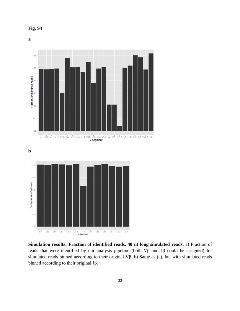
Figure S4 shows the fraction of simulated 37 nt sequences to which both a Vβ and a Jβ segment

could be assigned. Sequences are binned according to their original Vβ segment (Fig. S4a) or

their original Jβ segment (Fig. S4b). Figure S5 shows these results for simulated 77 nt reads.

These results show that on average, ~50% of the simulated 37 nt reads are assigned gene

segments. The un-assigned reads mostly correspond to simulated sequences with long CDR3

regions. The fraction of assigned reads grows to ~97% for the 77 nt long simulated sequences.

Loss of un-assigned sequences at the short length, however, does not lead to significant errors in

estimating the frequency of Jβ and Dβ gene segments, as assignment rate is very similar across

segments. Loss of un-assigned reads contributes error in estimating Vβ frequencies from 40 nt

reads, as some segments have a lower assignment rate.

The overall accuracy of our analysis according to the simulation is summarized in Figures S2

and S3. The correlations between predicted and observed V and J segment frequencies in the

simulation is very high (R2

> 0.98) for both read lengths. The following segments have an error

larger than 20%: Vβ 13, 16, 2, 4, 5.1/5.2, 6, 8.1, 9 (37 nt reads); Vβ 16, 5.1/5.2, 8.1 (77 nt reads).

Jβ frequencies show only a few percent error for both read lengths.

17

Supplementary figures and tables

Fig. S1

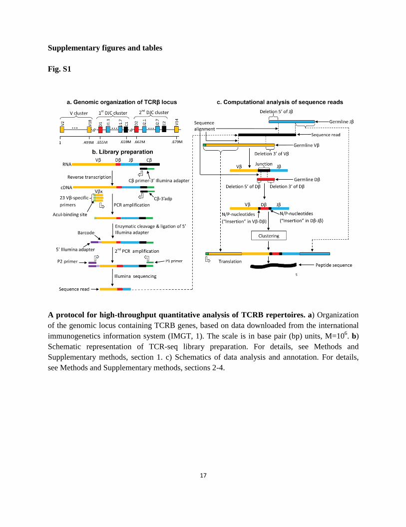
A protocol for high-throughput quantitative analysis of TCRB repertoires. a) Organization

of the genomic locus containing TCRB genes, based on data downloaded from the international

immunogenetics information system (IMGT, 1). The scale is in base pair (bp) units, M=106. b)

Schematic representation of TCR-seq library preparation. For details, see Methods and

Supplementary methods, section 1. c) Schematics of data analysis and annotation. For details,

see Methods and Supplementary methods, sections 2-4.

18

Fig. S2

a

b

19

c

Simulation results: TCRB gene segment usage obtained by running our analysis pipeline

on 40 nt long simulated reads. a) Vβ frequencies obtained, compared with the original

frequencies used in the simulation. b) Same as (a), for Jβ frequencies. c) Same as (a), for Dβ

frequencies.

20

Fig. S3

a

b

21

c

Simulation results: TCRB gene segment usage obtained by running our analysis pipeline

on 80 nt long simulated reads. a) Vβ frequencies obtained, compared with the original

frequencies used in the simulation. b) Same as (a), for Jβ frequencies. c) Same as (a), for Dβ

frequencies.

22

Fig. S4

a

b

Simulation results: Fraction of identified reads, 40 nt long simulated reads. a) Fraction of

reads that were identified by our analysis pipeline (both Vβ and Jβ could be assigned) for

simulated reads binned according to their original Vβ. b) Same as (a), but with simulated reads

binned according to their original Jβ.

23

Fig. S5

a

b

Simulation results: Fraction of identified reads, 80 nt long simulated reads. a) Fraction of

reads that were identified by our analysis pipeline (both Vβ and Jβ could be assigned) for

simulated reads binned according to their original Vβ. b) Same as (a), but with simulated reads

binned according to their original Jβ.

24

Fig. S6

10-4

10-3

10-2

10-1

100

10-4

10-2

100

PVD1

PV

D

2

b. VD2 vs. VD1 frequencies in selected clonotypes

R2=0.97

Slope=1.02

10-6

10-5

10-4

10-3

10-2

10-1

100

10-6

10-4

10-2

100

Normalized PVP

J

PV

J

a. VJ vs. VJ frequencies in unselected clonotypes

R2=0.99

Slope=0.99

Statistics of Vβ-Jβ and Vβ-Dβ pairing. a) Frequencies of individual Vβ and Jβ genes measured

in mice M1-M5 predict accurately frequencies of Vβ-Jβ gene pairs. The probability that a

unique, unselected clonotype carries a particular Vβ-Jβ gene pair (PVJβ) is plotted versus the

normalized product of the probability that it carries the Vβ (PVβ) and Jβ (PJβ). The average of

PVJβ in M1-M5 is not significantly different from the average of normalized PVβ× PJβ (p=0.67,

Wilcoxon signed rank test), consistent with statistical independence of Vβ and Jβ frequencies. A

linear fit to the data has a slope of 0.99, further supporting statistical independence. b)

Frequencies of Vβ-Dβ1 and Vβ-Dβ2 gene pairs measured in mice M1-M5 are very similar. The

probability that a unique, selected clonotype carries a particular Vβ paired with Dβ1 (PVDβ1) is

plotted versus the probability that it carries the same Vβ paired with Dβ2 (PVDβ2). Probabilities

were measured in datasets M1-M5, and are plotted on a log scale. The average of PVDβ1 in M1-

M5 is not significantly different from the average of PVDβ2 (p=0.06, Wilcoxon signed rank test).

Probabilities are plotted on a log scale. Colors in a,b represent the different mice, M1-M5.

25

Fig. S7

1.1 1.2 1.3 1.4 1.5 1.6 1.7 2.1 2.2 2.3 2.4 2.5 2.70

0.05

0.1

0.15

0.2 R2=0.84 (p<0.01)

J

PJ

a. Unselected clonotypes

1.1 1.2 1.3 1.4 1.5 1.6 1.7 2.1 2.2 2.3 2.4 2.5 2.70

0.1

0.2R2=0.83 (p<0.01)

J

PJ

c. Unselected clonotypes

M1-M5

Theory

1.1 1.2 1.3 1.4 1.5 1.6 1.7 2.1 2.2 2.3 2.4 2.5 2.70

0.05

0.1

0.15

0.2R2=0.79 (p<0.01)

J

PJ

d. Selected clonotypes

1.1 1.2 1.3 1.4 1.5 1.6 1.7 2.1 2.2 2.3 2.4 2.5 2.70

0.05

0.1

0.15

0.2R2=0.8 (p<0.01)

J

PJ

b. Selected clonotypes

CN 0 CN 10

Predictions of the biophysical model for Jβ frequencies are insensitive to cutoff used for

minimal clonotype size. a,b) Predicted Jβ frequencies (with parameters reported in the main

text) are compared with Jβ frequencies found in different subsets of unique unselected (a) and

selected (b) sequences with copy numbers greater than or equal to 0. c,d) Similar to a,b for

sequences with copy numbers greater than or equal to 10. The results show that the model’s

accuracy, as reported in the main text, is not sensitive to the copy number threshold.

26

Fig. S8

0 0.05 0.1 0.15 0.2 0.25-60

-50

-40

-30

-20

R2=0.1

R2=0.6 (without J1.4, 2.1)

J frequency

RIC

sco

re

a. R2 between mouse J frequencies and RIC scores

0 0.02 0.04 0.06 0.08 0.1 0.12 0.14 0.16 0.18-35

-30

-25

-20

R2=0.07

J frequency

RIC

sco

re

b. R2 between human J frequencies and RIC scores

Correlation between measured frequencies for mouse and human Jβ and RIC conservation

scores for individual Jβ RSSs. a,b) R2 values for (a) mouse and (b) human Jβ frequencies. The

R2 value is low for both sets of Jβ frequencies – for mouse, it increases greatly when two

outlying RIC scores, for Jβ1.4 and Jβ2.1, are removed. The plotted mouse and human Jβ

frequencies were averaged from the data found in Table S3,S6, respectively. RIC scores were

calculated for the following RSSs (19), using the method of Cowell et al. (20,21), as it is

implemented in RSSSite (21; http://itb.cnr.it/rss):

Mouse RSSs (order, J1.1-1.7,2.1-2.5,2.7): CACAGTGCCATAGGATGAGGAGAAAAAT, CACATCAGAATACAGATACTCGAATATG, CACAGCCTCCCGGGTCCACTTCAAAACC,

CACAACATTAAAGCCTGGTGGTAAAACT, CACAGTACAACATGAGGGTGACAAACTC,

CACAGCTGCAGGTGGCCTTGGTAAAACC, CACAACCCCTCCAGTCAGAAATGGAGC,

CACAGCAGAAAAGGGCTACCAAGAATTC, CACAGTCCTGGAAATGCTGGCACAAACC,

CACAGCCTCCAGGCTCAGGACAAAAACT, CACAGCCTCTTGGTACAGGACAAAAACT,

CACAGCCCCAGAACCCAACACAAAAAC, CACAGAGGCTCAACCCCACACACAAACC

Human RSSs (order: J1.1-1.6,2.1-2.7): CACAGTGACAGGGGTCAAGGTGAAAATC,

CACATAAGAATATAGCCACTCTAAAAGG, CACAGCCTCCCAGGGCCACTTCAAAACC,

CACAACATTAAAGACTGGAAGGAAAACC, CACAGTGCATCATGAGTGTGGCAAACCC,

CACAGCTGCAGAGGCTTAGATAAAACCC, CACAGTGGGAAGGGGCTGCCCAGAATTC,

CACAGCCCTGGGGACCCTGGCGCAAACC, CACAGCCTGGAGGCCCAGGACAAAAACC,

CACAGCCCCGAGACGCGGCACAGAAACT, CACGGCCCCCGAGCCCCGCACAAAAACC,

CACAGCCCGGGGACTCCCCGCAAAAACC, CACGGAGGTGCACCCCCGCATGCAAACC

27

Fig. S9

10-4

10-3

10-2

10-1

100

10-4

10-2

100

PJ

(selected CD4+)

PJ

(unsele

cte

d C

D4

+)

a. PJ

in unselected CD4+ clonotypes

R2=0.96

10-4

10-3

10-2

10-1

100

10-4

10-2

100

PJ

(selected CD4+)

PJ

(sele

cte

d C

D8

+)

b. PJ

in selected CD8+ clonotypes

R2=0.86

Jβ usage is similar among selected CD4+, unselected CD4

+ and selected CD8

+ repertoires. a)

Average probability that an unselected CD4+

clonotype carries a particular Jβ (PJβ) versus

average probability that a selected CD4+ clonotype carries the same Jβ. PJβ is based on M1-M5.

b) Average PJβ in selected CD8+

clonotypes versus average PJβ in selected CD4+ clonotypes. Two

CD8+

splenic T-cell libraries (denoted M7 & M8) were prepared for sequencing using the same

set of Vβ-specific PCR primers that were used for preparing M1-M4. Both libraries were

subsequently sequenced, and the resulting sequence reads were processed as described in

Methods. All average probabilities are plotted on a log scale. R2 is the squared correlation

coefficient between each pair of average probabilities being compared. Error bars indicate

standard deviations of the average probabilities.

28

Fig. S10

Significant numbers of amino acid sequences are shared among different individuals. a,b)

Measured number of selected (a) and unselected (b) amino acid (AA) sequences shared among

different subgroups of 5 mice (M1-M5). Shown are Venn diagrams which describe the number

of sequences that are exclusively shared among any subset of mice. Datasets were randomly

down-sampled to final sizes of 1.5×104 (a), and 2×10

3 (b) sequences, as in Figure 4 in the main

text.

29

Fig. S11

Sharing of Vβ genes in selected, public amino acid sequences. The Vβ gene for each public

amino acid (AA) sequence was defined as the Vβ of the dominant selected clonotype encoding

that AA sequence. The correlation coefficient between average gene frequencies in all versus in

public AA sequences is +0.83.

30

Fig. S12

Effect of sample size on sequence sharing. Unique amino-acid sequences from datasets M1-

M5 were sampled randomly, and the fraction of shared sequences were calculated for varying

sample sizes. The figure shows the fraction of shared sequences vs. sample size, for clones

shared between 2 datasets (purple), 3 datasets (magenta), 4 datasets (green) and all 5 datasets

(red).

31

Fig. S13

Distribution of Vβ/Jβ alignment lengths for permuted reads. 3×10

5 reads were randomly

selected from sequenced libraries, and their constituent nucleotides were permuted to randomize

their positions while keeping their frequencies constant. The best local alignment of each

permuted read to the germline Vβ sequences was determined. The best local alignment to the

germline Jβ sequences was similarly determined. Sequence alignments were done using the

ShortRead package (23). The lengths of these alignments were defined using the nmatch method.

a,b) Distribution of a) Vβ and b) Jβ alignment lengths for permuted reads of length 40 nt. c,d)

Distribution of c) Vβ and d) Jβ alignment lengths for permuted reads of length 80 nt.

32

Fig. S14

Fit of model to observed plasmid copy number for estimation of primer bias. Different

groups of plasmids found in three control libraries were diluted by different amounts (see above).

Plasmids in control libraries 2 and 3 were sequenced using the same set of 23 Vβ primers (Table

S9, column 3), whereas plasmids in control library 1 were sequenced using a different set of Vβ

primers that partially overlapped with the former set (Table S9, column 2). We determined both

the observed and the expected copy number of each plasmid as described in Supplementary

methods. a) The expected copy number of each plasmid is plotted against the observed copy

number, and b) Plasmids were grouped according to their Vβ (~3 plasmids per Vβ). The average

expected copy number of plasmids carrying each Vβ is plotted against the average observed copy

number for that Vβ.

33

Fig. S15

2 4 16 10 1 5.28.35.18.28.1 13 12 11 9 6 15 19 20 17 3.1 7 18 140

0.1

0.2

0.3

V

PV

a. V frequency in unique seqs. with CN 0

1.1 1.2 1.3 1.4 1.5 1.6 1.7 2.1 2.2 2.3 2.4 2.5 2.70

0.1

0.2

J

PJ

e. J frequencies in unique seqs. with CN 5

1.1 1.2 1.3 1.4 1.5 1.6 1.7 2.1 2.2 2.3 2.4 2.5 2.70

0.1

0.2

J

PJ

d. J frequencies in unique seqs. with CN 0

2 4 16 10 1 5.28.35.18.28.1 13 12 11 9 6 15 19 20 17 3.1 7 18 140

0.2

0.4

V

PV

c. V frequencies in unique seqs. with CN 10

2 4 16 10 1 5.28.35.18.28.1 13 12 11 9 6 15 19 20 17 3.1 7 18 140

0.1

0.2

0.3

V

PV

b. V frequencies in unique seqs. with CN 5

1.1 1.2 1.3 1.4 1.5 1.6 1.7 2.1 2.2 2.3 2.4 2.5 2.70

0.1

0.2

J

PJ

f. J frequencies in unique seqs. with CN 10

M1 M2 M3 M4 M5

Effect of the cutoff for minimal cluster size on estimating usage of Vβ and Jβ genes. a-c)

Measured frequency of Vβ gene usage (PVβ) for selected sequences, with at least 0/5/10 copies,

from mice M1-M5. d-f) Measured frequency of Jβ gene usage (PJβ) for selected sequences, with

at least 0/5/10 copies, from mice M1-M5.

34

Fig. S16

10-6

10-5

10-4

10-3

10-2

10-1

100

10-6

10-5

10-4

10-3

10-2

10-1

100

PVJ

PV

J (

rep

ea

t)

VJ frequencies in technical repeat of M2

R2=1

The sequencing reaction does not substantially bias Vβ-Jβ frequencies. Vβ-Jβ frequencies in

unique reads from M2 are plotted against corresponding frequencies from a technical replicate of

the same library. Dotted red lines trace the boundaries of a 2-fold difference between Vβ-Jβ

frequencies.

35

Fig. S17

The biophysical model has a statistically significant fit to Dβ-Jβ frequencies. a,b) Shown are

histograms of R2 values obtained by fitting the model to 200 separate random permutations of all

26 possible averaged Dβ-Jβ frequencies found in (a) all unselected clonotypes from datasets M1-

M5 (Table S3), and (b) in unselected clonotypes from datasets M1-M5 that carry the Vβ17 gene.

The red line indicates the R2 value obtained by fitting the model to the non-permuted empirical

frequencies.

0 0.1 0.2 0.3 0.4 0.5 0.6 0.7 0

10

20

30

40

50

60

R 2

value

a. 26 D -J frequencies found in all unique clonotypes

0 0.1 0.2 0.3 0.4 0.5 0.6 0.7 0

20

40

60

80

R 2 value

Frequency

b. 26 D -J frequencies found in unique V 17 + clonotypes

Frequency

36

Table S1

Number of all sequences and of clonotypes found in each mouse dataset

Dataset

Total

seqs

(×104)

Unique

seqs

(×104)

% In-

frame

seqs

(non-

Vβ17) ≠

In-frame

unique seqs

with

identifiable

CDR3*

(×104)

In-frame seqs

with

identifiable

Dβ**

(×104)

Ratio of

in-frame

seqs with

Dβ1 vs.

Dβ2

In-frame

seqs with ≤2

cleavage

errors & ≥5

copies†

(×104)

M1 51.8 16.5 96.6 13.8 4.0 1.21 2.6

M2 70.2 11.9 97.0 9.7 2.9 1.11 2.9

M3 103.6 23.7 96.0 19.9 6.1 1.23 4.9

M4 112.8 10.9 96.5 9.1 2.6 1.14 2.9

M5 488.5 76.7 97.0 67.7 33.3 0.81

15.7

M6

(Tech.

repeat of

M2)

141.9 11.8 96.4 9.9 2.9 1.17

3.4

M7

(CD8) 117.9 30.3 97.2 26.9 8.5

1.32 5.3

M8

(CD8) 104.7 27.9 97.0 24.6 8.3

1.10 4.5

≠The fraction of non-Vβ17

+ sequences that do not have a stop codon within the Vβ-Dβ-Jβ region.

*The CDR3 region is defined as starting from the last conserved cysteine of Vβ and ending at the

first position of the conserved amino acid motif [F|H][A|G]XG of Jβ, where X denotes any

amino acid.

**Dβ is identified based on a perfect alignment, of length ≥7nt, between each clonotype’s

junctional sequence and the germline sequence of either Dβ1 (GGGACAGGGGGC) or Dβ2

(GGGACTGGGGGGGC), downloaded from the international immunogenetics information

system (IMGT; 1). A clonotype is assigned Dβ1 (or Dβ2) if the optimal alignment to Dβ1 (or

Dβ2) is longer.

†These sequences are defined as clonotypes. Consensus cleavage site is defined as starting at the

consensus/median start position of the optimal alignment between each clonotype and its

germline Vβ. Table entry shows the number of unique sequences with an error in cleavage

position that is ≤ 2 bp and with a bias-corrected copy number of ≥5.

37

Table S2

Vβ frequencies measured using antibodies and flow cytometry

Vβ A1 A2 A3

V2 0.056601 0.0627725 0.049448

V3.1 0.0048288 0.00506295 0.0052824

V4 0.0808695 0.0877735 0.0639295

V5 0.03204 0.042333 0.032979

V6 0.082556 0.084999 0.073962

V7 0.037585 0.041816 0.0342695

V8.1/8.2 0.1673035 0.1667365 0.159465

V8.3 0.0575735 0.060769 0.048198

V9 0.011638 0.00965315 0.011694

V10 0.045047 0.0416165 0.0290695

V11 0.073881 0.06331 0.054061

V12 0.046149 0.0339605 0.027298

V13 0.020563 0.0156045 0.0147305

V14 0.092645 0.0802185 0.074215

V17 0.0047519 0.004342 0.00566275

CD4+ T cells were isolated from spleens of three C57BL/6 mice (A1-A3), at ages matched to

those in datasets M1-M8. Cells were stained with a set of fluorescently labeled monoclonal

antibodies to 15 different mouse Vβ chains. Table shows the fraction of cells that were positive

for expression of each Vβ.

38

Table S3

Occurrence of Dβ-Jβ pairings in unselected clonotypes from M1-M5

Jβ M1 M2 M3 M4 M5

Dβ1 Dβ2 Dβ1 Dβ2 Dβ1 Dβ2 Dβ1 Dβ2 Dβ1 Dβ2

1.1 56 3 102 4 83 6 83 5 317 5

1.2 42 1 84 0 68 8 45 3 194 2

1.3 32 0 37 3 32 2 31 3 107 0

1.4 12 0 31 2 36 3 23 0 95 2

1.5 7 3 16 0 16 0 10 0 49 0

1.6 19 0 30 7 52 0 22 6 60 0

1.7 0 0 0 0 0 0 0 0 0 0

2.1 86 87 161 126 159 100 131 107 534 537

2.2 40 25 59 41 66 42 60 28 209 123

2.3 50 75 86 91 89 72 63 58 241 269

2.4 69 59 109 95 72 70 67 75 238 252

2.5 78 62 113 116 102 97 86 111 227 300

2.7 120 90 159 145 150 110 161 136 527 603

Total 611 405 987 630 925 510 782 532 2798 2093

39

Table S4

RS positions for mouse Dβ-Jβ genes

Dβ/Jβ RS position Dβ/Jβ RS position Dβ/Jβ RS position

D1 655165 J1.4 656735 J2.2 664871

D2 664119 J1.5 657008 J2.3 665137

J1.1 655788 J1.6 657478 J2.4 665276

J1.2 655925 J1.7 657567 J2.5 665368

J1.3 656247 J2.1 664668 J2.7 665724

RS positions are based on the IMGT annotation (1) of the mouse TCRB locus.

40

Table S5

Variation of parameter estimates for the biophysical model

Dataset

Parameter estimates (95% Confidence intervals) and R2 values

for predicted Jβ frequencies

b c R2

M1 59.7579 (28.8856,

90.6271) 10.7999 (10.5275, 11.0724)

0.8649

M2 73.6460 (30.7887,

116.4973) 10.8518 (10.5129, 11.1907)

0.8122

M3 71.1065 (31.3525,

110.8635) 10.8489 (10.5080, 11.1899)

0.8100

M4 62.8383 (33.9056,

91.7767) 10.8525 (10.4588, 11.2462)

0.8433

M5 72.9176 (19.1983,

133.2636) 10.9552 (10.4537, 11.5467)

0.7708

Average*

of M1-

M5

68.7666 (33.8653,

103.6809) 10.8589 (10.4897, 11.2283)

0.8279

Average*

of M7-

M8

(CD8)

88.4425 (39.1503,

137.7357) 10.8911 (10.5631, 11.2192)

0.7507

The biophysical model for gene rearrangement frequency was fit to Dβ-Jβ frequencies in

unselected clonotypes (Table S3) using the RS positions given in Table S4.

*The average relative frequencies of Dβ-Jβ frequencies found in the indicated mouse datasets.

41

Table S6

Occurrence of Dβ-Jβ pairings in selected clonotypes from M1-M5, and Jβ frequencies in a

published dataset

Jβ M1 M2 M3 M4 M5 N

Dβ1 Dβ2 Dβ1 Dβ2 Dβ1 Dβ2 Dβ1 Dβ2 Dβ1 Dβ2 Dβ1& Dβ2

1.1 1234 23 939 15 1850 53 858 17 5365 131

0.0865

1.2 641 23 583 20 1063 18 560 8 3138 71

0.0364

1.3 405 14 421 10 730 21 325 11 1785 41

0.0244

1.4 546 20 433 28 870 54 387 24 2334 35

0.0288

1.5 276 11 218 15 549 10 172 5 1376 18

0.0115

1.6 242 8 257 11 496 20 256 7 1403 29

0.0178

1.7 2 2 3 4 3 6 2 7 0 0

0

2.1 1131 1374 1092 1376 1986 2388 1004 1231 6795 11792

0.1679

2.2 545 441 469 459 1007 815 388 343 2798 2873

0.0404

2.3 747 1087 718 1007 1200 1852 621 851 3179 6400

0.1353

2.4 693 1276 713 1138 1235 2148 618 1049 3734 8313

0.0767

2.5 1233 1779 1073 1594 2116 2992 1068 1473 4749 10032

0.1631

2.7 1481 1915 1463 1735 2348 3229 1371 1676 8559 16156

0.2114

Total 9176 7973 8382 7412 15453 13606 7630 6702 45215 55891

1

Dataset N consists of a total of ~600 transcripts, including non-expressed Vβ17b+ transcripts

from C57 BL/6 mice, and expressed Vβ17a+

transcripts from both SJL mice and an SJL mouse

variant lacking T cells that are specific for the E complex. The dataset was extracted from

Figure 1A of (3).

42

Table S7

Frequencies of Jβ genes from datasets H1-H5

Jβ Probability

H1 H2 H3 H4 H5

1.1 0.1356 0.1743 0.1985 0.2174 0.1659

1.2 0.0859 0.0896 0.0874 0.0802 0.0413

1.3 0.0215 0.0363 0.0413 0.0316 0.0146

1.4 0.0335 0.0654 0.0680 0.0632 0.0413

1.5 0.0793 0.0533 0.0510 0.0437 0.0146

1.6 0.0349 0.0533 0.0583 0.0437 0.0243

2.1 0.1706 0.1138 0.1020 0.1288 0.1897

2.2 0.0776 0.1114 0.1336 0.1069 0.2164

2.3 0.1134 0.0944 0.0923 0.0608 0.1386

2.4 0.0171 0.0097 0.0121 0.0073 0.0049

2.5 0.0903 0.0387 0.0291 0.0170 0.0122

2.6 0.0164 0.0194 0.0243 0.0146 0.0438

2.7 0.1239 0.1404 0.1020 0.1847 0.0924

Dataset H1 (Table S1 of Ref. 24) contains CDR3 transcripts from mostly antigen-experienced

human T cells, while H2-H5 contain CDR3 genomic sequences from CD4+CD45RO

-,

CD4+CD45RO

+, CD8

+CD45RO

-, and CD8

+CD45RO

+ human T cells, respectively. The latter

datasets were extracted from Figure 4 of (25).

43

Table S8

RS positions for human Dβ-Jβ genes

Dβ/Jβ RS position Jβ RS position Dβ/Jβ RS position

D1 187957 J1.4 189929 J2.3 198551

D2 197453 J1.5 190202 J2.4 198702

J1.1 188584 J1.6 190692 J2.5 198823

J1.2 188721 J2.1 198069 J2.6 198943

J1.3 189334 J2.2 198264 J2.7 199160

RS positions are based on the IMGT annotation (1) of the human TCRB locus.

44

Table S9

PCR primers and related PCR bias

Vβ Sequence

Bias*

Expt. 1 Expt. 2 Expt. 1 Expt. 2

V1 gactcagctgtctatttttgtgc Same 0.2907 0.2982

V2 ccagggcagaaccttgtact Same 0.7406 0.7597

V3.1 gactcagcactgtacctctgtg Same 0.7756 0.7956

V4 gatgactcggccacatacttc gactcggccacatacttctg 0.3940 0.6209

V5.1 tagaggactctgccgtgtact Same 5.6119 5.7568

V5.2 aactggaggactctgctatgtact Same 2.0057 2.0574

V6 cgagatggccgtttttctct Same 0.7351 0.7541

V7 cagacatctgtgtacttctgtgct ccagacatctgtgtacttctgtgc 1.8538 2.5222

V8.1 cagacagctgtatatttctgtgcc Same 0.7637 0.7834

V8.2 cagacatcagtgtacttctgtgcc ctcagacatcagtgtacttctgtg 0.0540 0.7234

V8.3 tcagacatctttgtacttctgtgc Same 0.7789 0.7990

V9 attctgccatgtacctctgtg ttctgccatgtacctctgtg 0.6155 0.2113

V10 gactctgctgtgtatctctgtgc Same 0.4599 0.4718

V11 gactcagcggtgtatctttgtg Same 0.6545 0.6714

V12 gactcagctgtgtatctgtgtgc Same 0.4653 0.4773

V13 ggcgacacagccacctatc cgacacagccacctatctctg 0.7760 0.2102

V14 gccactctggcttctacctc Same 0.7994 0.8200

V15 gaagacagaggcttatatctctg tgaagacagaggcttatatctctg 1.4723 0.4173

V16 gactcagctgtgtacttctgtgc Same 0.8485 0.8704

V17 gactcagcactgtagctctgtg Same 0.6300 0.6463

45

V18 ggagacagcagtatctatttctg Same 0.2006 0.2058

V19 gattcagctgtgtacttctgtgc Same 1.4478 1.4851

V20 gactcagcactgtacttgtgctc Same 1.1864 0.6424

*The bias for each primer was determined as described above in Supplementary methods,

sections 5 & 9. It depends on the different primers used in each experiment.

References

1. LeFranc MP, et al. (2009) IMGT, the international immunogenetics information system.

Nucleic Acids Res 37:D1006-D1012.

2. Smith TF, Waterman MS (1981) Identification of common molecular subsequences. J

Mol Biol 147:195-197.

3. Candéias S, Waltzinger C, Benoist C, Mathis D (1991) The Vβ17+ T cell repertoire,

skewed Jβ usage after thymic selection; dissimilar CDR3s in CD4+ versus CD8

+ cells. J

Exp Med 174:989-1000.

4. Wade T, Bill J, Marrack P, Palmer E, Kappler JW (1988) Molecular basis for the

nonexpression of Vβ17 in some strains of mice. J Immunol 141:2165-2167.

5. Dekker J, Rippe K, Dekker M, Kleckner N (2002) Capturing chromosome conformation.

Science 295:1306-1311.

6. Styblinski MA, Tang TS (1990) Experiments in non-convex optimization, stochastic

approximation with function smoothing and simulated annealing. Neur Net 3:467-483.

7. Wilf HA (1994) Generating functionology (Academic Press Inc, Philadelphia, USA).

8. Gardiner CW (2004) Handbook of Stochastic Methods for Physics, Chemistry and the

Natural Sciences (Springer, Berlin, Germany).

9. Manfras BJ, Terjung D, Boehm BO (1999) Non-productive human TCR beta chain genes

represent V-D-J diversity before selection upon function: insight into biased usage of

TCRBD and TCRBJ genes and diversity of CDR3 region length. Hum Immunol 60:1090-

1100.

10. Robins HS, et al. (2010) Overlap and effective size of the human CD8+ T cell receptor

repertoire. Science Transl Med 2:47ra64.

11. Maes J, et al. (2006) Activation of V(D)J recombination at the IgH chain JH locus occurs

within a 6-kilobase chromatin domain and is associated with nucleosomal remodeling. J

Immunol 176:5409-5417.

12. Osipovic OA, et al. (2007) Essential function for SWI-SNF chromatin-remodeling

complexes in the promoter-directed assembly of Tcrb genes. Nat Immunol 8:809-816.

46

13. Coté J, Peterson CL, Workman JL (1998) Perturbation of nucleosome core structure by

the SWI/SNF complex persists after its detachment enhancing subsequent transcription

factor binding. Proc Natl Acad Sci USA 95:4947-4952.

14. Kwon J, et al. (2000) Histone acetylation and hSWI/SNF remodeling act in concert to

stimulate V(D)J cleavage of nucleosomal DNA. Mol Cell 6:1037-1048.

15. Golding A, et al. (1999) Nucleosome structure completely inhibits in vitro cleavage by

the V(D)J recombinase. EMBO J 18:3712-3723.

16. Ringrose L, Chabanis S, Angrand PO, Woodroofe C, Stewart AF (1999) Quantitative

comparison of DNA looping in vitro and in vivo, chromatin increases effective DNA

flexibility at short distances. EMBO J 18:6630-6641.

17. van Gent DC, Hiom K, Paull TT, Gellert M (1997) Stimulation of V(D)J cleavage by

high mobility group proteins. EMBO J 16:2665-2670.

18. McCauley M, Hardwidge PR, Maher III LJ, Williams MC (2005) Dual binding modes for

an HMG domain from human HMGB2 on DNA. Biophys J 89:353-364.

19. LeFranc MP, et al. (2009) IMGT, the international immunogenetics information system.

Nucleic Acids Res 37:D1006-D1012.

20. Cowell LG, Davila M, Yang K, Kepler TB, Kelsoe G (2003) Prospective estimation of

recombination signal efficiency and identification of functional cryptic signals in the

genome by statistical modeling. J Exp Med 197:207-220.

21. Lee A F, et al. (2003) A functional analysis of the spacer of V(D)J recombination signal

sequences. PLoS Biol 1:e1.

22. Merelli I, et al. (2010) RSSSite, a reference database and prediction tool for the

identification of cryptic recombination signal sequences in human and murine genomes.

Nucleic Acids Res 38:W262-W267.

23. Morgan M, et al. (2009) ShortRead, a bioconductor package for input quality assessment

and exploration of high-throughput sequence data. Bioinformatics 25:2607-2608.

24. Freeman JD, Warren RL, Webb JR, Nelson BH, Holt RA (2009) Profiling the T-cell

receptor beta-chain repertoire by massively parallel sequencing. Genome Res 19:1817-

1824.

25. Robins HS, et al. (2009) Comprehensive assessment of T-cell receptor β-chain diversity

in αβ T cells. Blood 114:4099-4107.