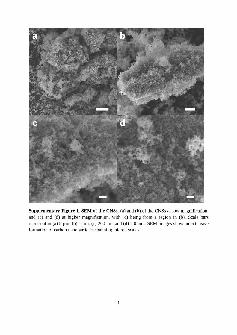
1

Supplementary Figure 1. SEM of the CNSs. (a) and (b) of the CNSs at low magnification,

and (c) and (d) at higher magnification, with (c) being from a region in (b). Scale bars

represent in (a) 5 µm, (b) 1 µm, (c) 200 nm, and (d) 200 nm. SEM images show an extensive

formation of carbon nanoparticles spanning micron scales.

2

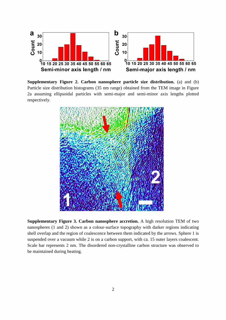
Supplementary Figure 2. Carbon nanosphere particle size distribution. (a) and (b)

Particle size distribution histograms (35 nm range) obtained from the TEM image in Figure

2a assuming ellipsoidal particles with semi-major and semi-minor axis lengths plotted

respectively.

Supplementary Figure 3. Carbon nanosphere accretion. A high resolution TEM of two

nanospheres (1 and 2) shown as a colour-surface topography with darker regions indicating

shell overlap and the region of coalescence between them indicated by the arrows. Sphere 1 is

suspended over a vacuum while 2 is on a carbon support, with ca. 15 outer layers coalescent.

Scale bar represents 2 nm. The disordered non-crystalline carbon structure was observed to

be maintained during heating.

3

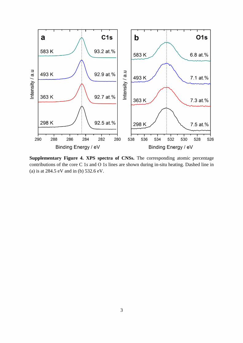
Supplementary Figure 4. XPS spectra of CNSs. The corresponding atomic percentage

contributions of the core C 1s and O 1s lines are shown during in-situ heating. Dashed line in

(a) is at 284.5 eV and in (b) 532.6 eV.

4

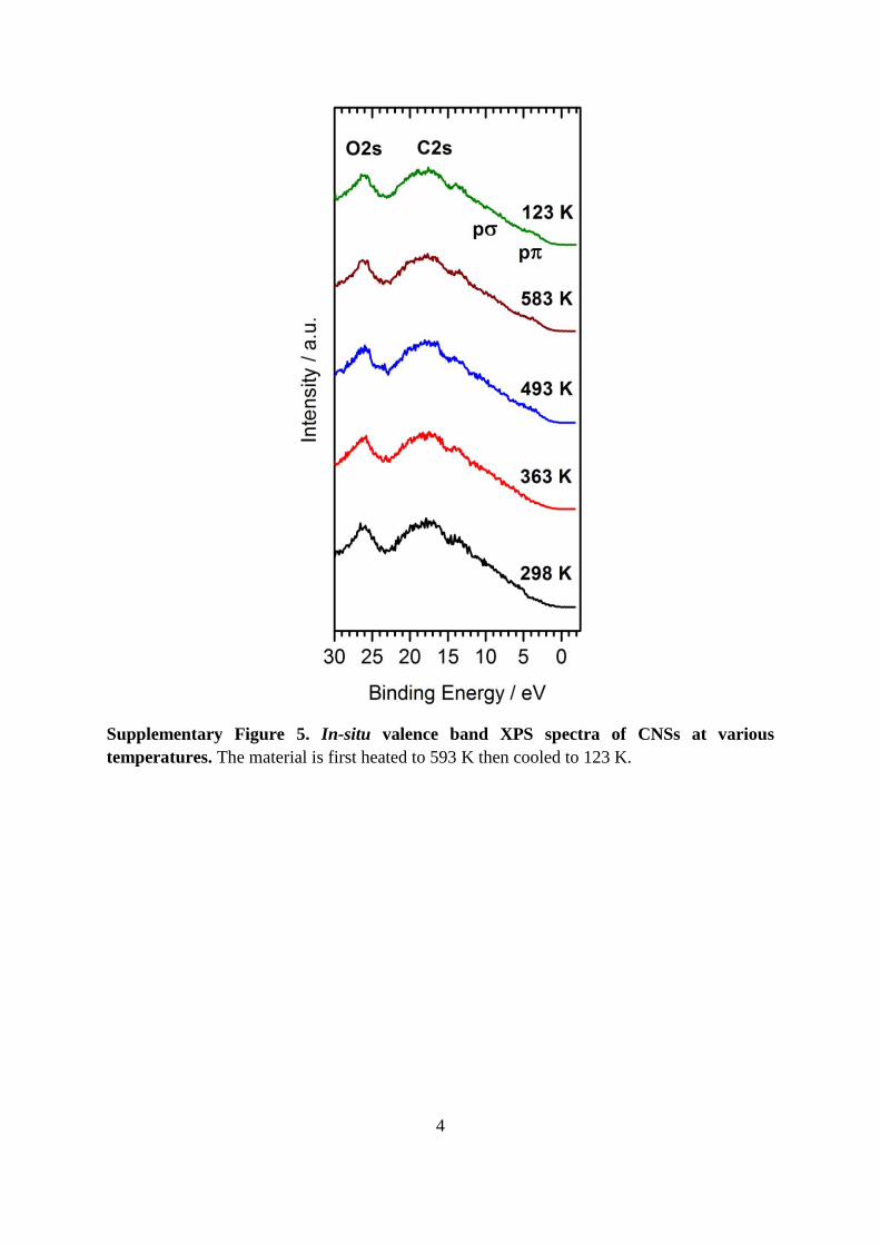
Supplementary Figure 5. In-situ valence band XPS spectra of CNSs at various

temperatures. The material is first heated to 593 K then cooled to 123 K.

5

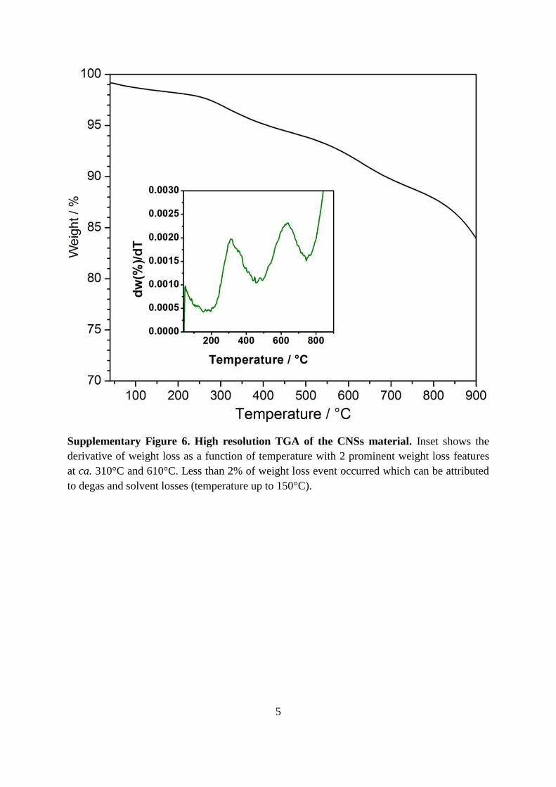
Supplementary Figure 6. High resolution TGA of the CNSs material. Inset shows the

derivative of weight loss as a function of temperature with 2 prominent weight loss features

at ca. 310°C and 610°C. Less than 2% of weight loss event occurred which can be attributed

to degas and solvent losses (temperature up to 150°C).

6

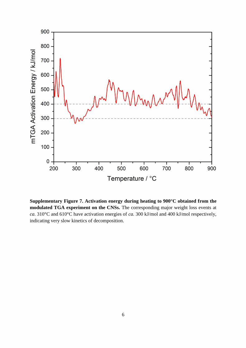
Supplementary Figure 7. Activation energy during heating to 900°C obtained from the

modulated TGA experiment on the CNSs. The corresponding major weight loss events at

ca. 310°C and 610°C have activation energies of ca. 300 kJ/mol and 400 kJ/mol respectively,

indicating very slow kinetics of decomposition.

7

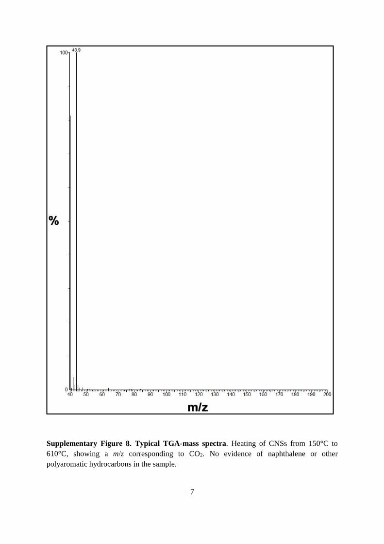
Supplementary Figure 8. Typical TGA-mass spectra. Heating of CNSs from 150°C to

610°C, showing a m/z corresponding to CO2. No evidence of naphthalene or other

polyaromatic hydrocarbons in the sample.

8

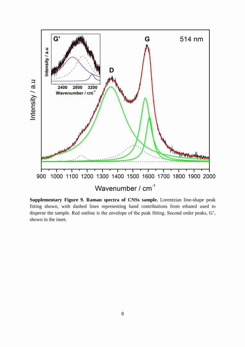
Supplementary Figure 9. Raman spectra of CNSs sample. Lorentzian line-shape peak

fitting shown, with dashed lines representing band contributions from ethanol used to

disperse the sample. Red outline is the envelope of the peak fitting. Second order peaks, G’,

shown in the inset.

9

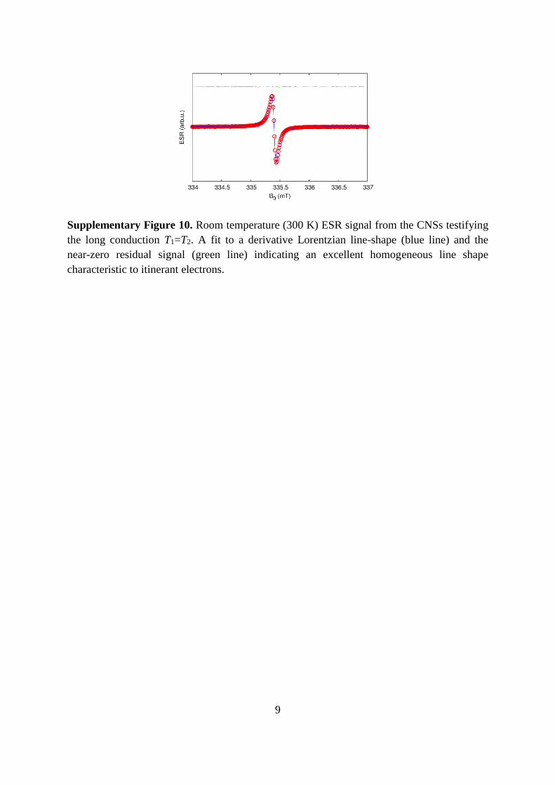
Supplementary Figure 10. Room temperature (300 K) ESR signal from the CNSs testifying

the long conduction T1=T2. A fit to a derivative Lorentzian line-shape (blue line) and the

near-zero residual signal (green line) indicating an excellent homogeneous line shape

characteristic to itinerant electrons.

10

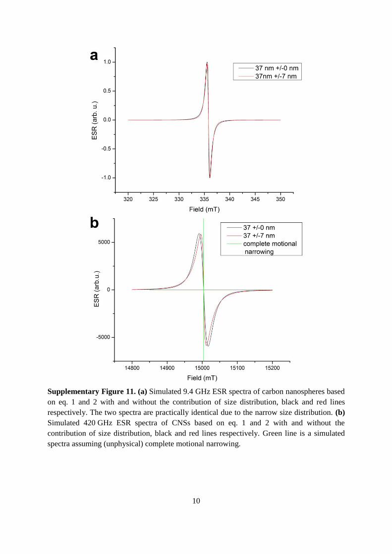
Supplementary Figure 11. (a) Simulated 9.4 GHz ESR spectra of carbon nanospheres based

on eq. 1 and 2 with and without the contribution of size distribution, black and red lines

respectively. The two spectra are practically identical due to the narrow size distribution. (b)

Simulated 420 GHz ESR spectra of CNSs based on eq. 1 and 2 with and without the

contribution of size distribution, black and red lines respectively. Green line is a simulated

spectra assuming (unphysical) complete motional narrowing.

11

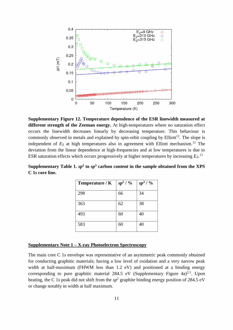
Supplementary Figure 12. Temperature dependence of the ESR linewidth measured at

different strength of the Zeeman energy. At high-temperatures where no saturation effect

occurs the linewidth decreases linearly by decreasing temperature. This behaviour is

commonly observed in metals and explained by spin-orbit coupling by Elliott12. The slope is

independent of EZ at high temperatures also in agreement with Elliott mechanism.12 The

deviation from the linear dependence at high-frequencies and at low temperatures is due to

ESR saturation effects which occurs progressively at higher temperatures by increasing EZ.13

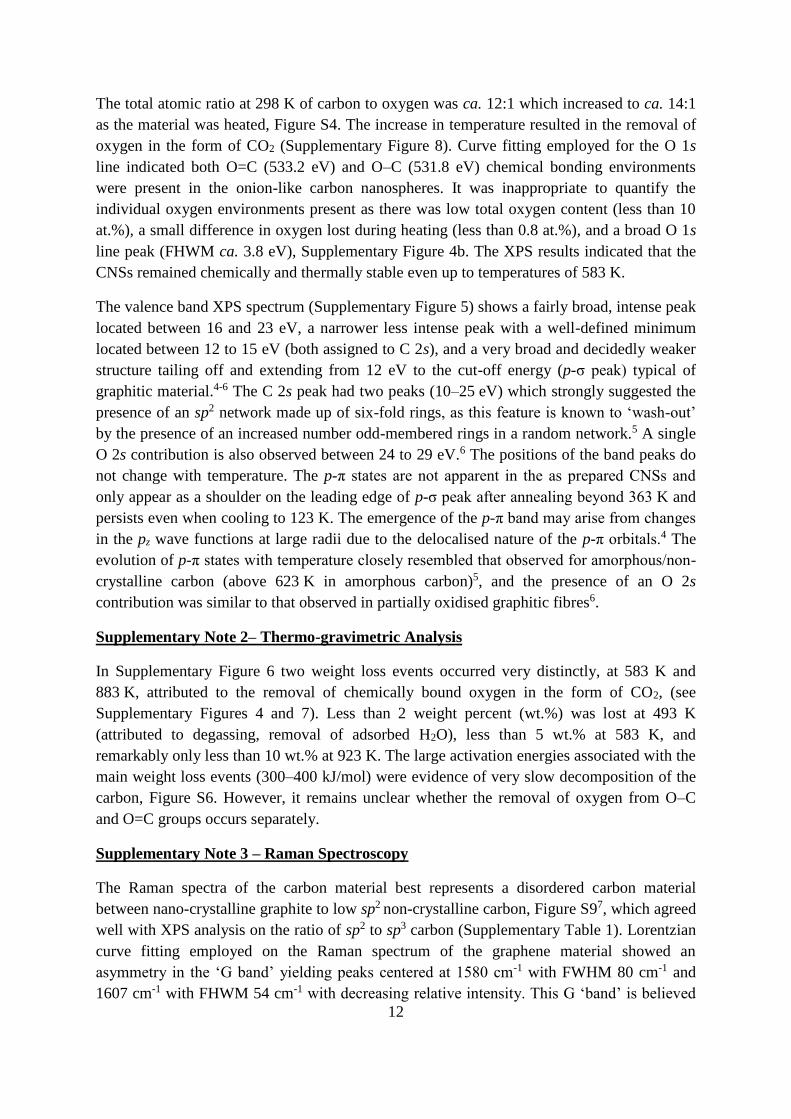
Supplementary Table 1. sp2 to sp3 carbon content in the sample obtained from the XPS

C 1s core line.

Temperature / K sp2 / % sp3 / %

298 66 34

363 62 38

493 60 40

583 60 40

Supplementary Note 1 – X-ray Photoelectron Spectroscopy

The main core C 1s envelope was representative of an asymmetric peak commonly obtained

for conducting graphitic materials; having a low level of oxidation and a very narrow peak

width at half-maximum (FHWM less than 1.2 eV) and positioned at a binding energy

corresponding to pure graphitic material 284.5 eV (Supplementary Figure 4a)2,3. Upon

heating, the C 1s peak did not shift from the sp2 graphite binding energy position of 284.5 eV

or change notably in width at half maximum.

12

The total atomic ratio at 298 K of carbon to oxygen was ca. 12:1 which increased to ca. 14:1

as the material was heated, Figure S4. The increase in temperature resulted in the removal of

oxygen in the form of CO2 (Supplementary Figure 8). Curve fitting employed for the O 1s

line indicated both O=C (533.2 eV) and O–C (531.8 eV) chemical bonding environments

were present in the onion-like carbon nanospheres. It was inappropriate to quantify the

individual oxygen environments present as there was low total oxygen content (less than 10

at.%), a small difference in oxygen lost during heating (less than 0.8 at.%), and a broad O 1s

line peak (FHWM ca. 3.8 eV), Supplementary Figure 4b. The XPS results indicated that the

CNSs remained chemically and thermally stable even up to temperatures of 583 K.

The valence band XPS spectrum (Supplementary Figure 5) shows a fairly broad, intense peak

located between 16 and 23 eV, a narrower less intense peak with a well-defined minimum

located between 12 to 15 eV (both assigned to C 2s), and a very broad and decidedly weaker

structure tailing off and extending from 12 eV to the cut-off energy (p-σ peak) typical of

graphitic material.4-6 The C 2s peak had two peaks (10–25 eV) which strongly suggested the

presence of an sp2 network made up of six-fold rings, as this feature is known to ‘wash-out’

by the presence of an increased number odd-membered rings in a random network.5 A single

O 2s contribution is also observed between 24 to 29 eV.6 The positions of the band peaks do

not change with temperature. The p-π states are not apparent in the as prepared CNSs and

only appear as a shoulder on the leading edge of p-σ peak after annealing beyond 363 K and

persists even when cooling to 123 K. The emergence of the p-π band may arise from changes

in the pz wave functions at large radii due to the delocalised nature of the p-π orbitals.4 The

evolution of p-π states with temperature closely resembled that observed for amorphous/non-

crystalline carbon (above 623 K in amorphous carbon)5, and the presence of an O 2s

contribution was similar to that observed in partially oxidised graphitic fibres6.

Supplementary Note 2– Thermo-gravimetric Analysis

In Supplementary Figure 6 two weight loss events occurred very distinctly, at 583 K and

883 K, attributed to the removal of chemically bound oxygen in the form of CO2, (see

Supplementary Figures 4 and 7). Less than 2 weight percent (wt.%) was lost at 493 K

(attributed to degassing, removal of adsorbed H2O), less than 5 wt.% at 583 K, and

remarkably only less than 10 wt.% at 923 K. The large activation energies associated with the

main weight loss events (300–400 kJ/mol) were evidence of very slow decomposition of the

carbon, Figure S6. However, it remains unclear whether the removal of oxygen from O–C

and O=C groups occurs separately.

Supplementary Note 3 – Raman Spectroscopy

The Raman spectra of the carbon material best represents a disordered carbon material

between nano-crystalline graphite to low sp2 non-crystalline carbon, Figure S97, which agreed

well with XPS analysis on the ratio of sp2 to sp3 carbon (Supplementary Table 1). Lorentzian

curve fitting employed on the Raman spectrum of the graphene material showed an

asymmetry in the ‘G band’ yielding peaks centered at 1580 cm-1 with FWHM 80 cm-1 and

1607 cm-1 with FHWM 54 cm-1 with decreasing relative intensity. This G ‘band’ is believed

13

to be due to the in-plane stretching motion between pairs of sp2 carbon atoms. This mode

does not require the presence of six-fold rings, so it occurs at all sp2 sites not only those in

rings, and appears in the range 1500–1630 cm-1. The asymmetry in the peak may be caused

by doping of the graphitic layers by ethanol present which was used to disperse the sample

prior to measurement8.

The presence of the ‘D band’ centered at 1355 cm-1 with FWHM 230 cm-1, is believed to be

related to the number of ordered aromatic rings, and affected by the probability of finding a

six-fold ring in a cluster. The second order peaks (G’) are not well defined, but appear as a

small modulated bump between 2200 and 3500 cm-1 and best represent a multi-layer

graphitic material in the presence of some ethanol.

The intensity ratio of the D band to the G band(s) value, commonly reported as ID/IG, was 1.2

and 1.7, indicating a significant number of defect sites present.7,9 This value compares well

with reported ID/IG values for carbon nanospheres, which range between 0.8–1.2.10 The

relative intensity and positions of the G and D bands have been interpreted to be due to the

presence of defects and disorder in the short range graphitic fragments.11 This is directly

verified with TEM (Figure 3 and Supplementary Figure 3). The identification of bands

associated with other phases, which may also be present in smaller quantities (e.g. diamond),

was not possible due to the background of the Raman spectrum contributions of disordered

carbon.

Supplementary Note 4 – Electron Spin Resonance

ESR experiments revealed a presence of a single narrow (ΔH=0.05 mT) Lorentzian line with

g=2.00225 at 9.4 GHz frequency (Supplementary Figure 10). The spectral resolution of ESR

is proportional to the frequency. The deviations from the Lorentzian shape even at 420 GHz

were smaller than 5%. There was no g-factor anisotropy observed within the resolution of the

420 GHz measurements of Δg<10-6. Note that in carbon the g-factor values of localized

paramagnetic centres are in the 2.0025-2.0050 range with anisotropies Δg in the order of

~510-4.1

A spin-½ system in magnetic field B0 is a two-level quantum system which can be a physical

representation of a qubit. If an oscillating magnetic field is applied in such that the total

magnetic field B acting on the spin is B=B0z+B1(sin(ωt)x+cos(ωt)y) the qubit will oscillate

between the states |+½> and |-½>. Let the q-bit be in state |-½> at t=0. The probability to find

the q-bit in state |+½> at time t is

P(t) = (ω1/Ω)2sin2(Ωt/2)

where Ω = √(ω-ω0)2 + ω1

2 ; and ω0 = γB0, ω1 = γB1, and γ is the gyromagnetic ratio.

This is called Rabi oscillation. Thus the detected Rabi oscillations of several cycles can be

taken as evidence that the system allows the deliberate preparation of any superposition of a

two level spin-½ system. For example, to go from one state |+½> to |-½> we can adjust the

time t during which the oscillating field acts such that ω1t/2 = π/2 (i.e. t = π/ω1); this is called

14

a π pulse. If a time intermediate between 0 and π/ω1 is chosen, e.g. in the case for t = π/2ω1,

we obtain a π/2 pulse, and this results in a superposition of √2*(|+½> + |-½>) of the two

states.

For conduction electron spin based qubits the size distribution on the ESR relaxation rate has

little effect. This is in contrasting difference from localized paramagnetic spin based q-bits

like N@C60 N-V centers or other molecular magnet based systems. The ESR relaxation at

EZ=0 is limited by T1 because the motional narrowing of conduction electrons is complete.

Thus the ESR line is homogeneous and independent of the size distribution. Inhomogeneous

broadening comes about at high magnetic fields. The complete motional narrowing of

conduction electrons breaks down as electrons progressively confine to cyclotron orbits. This

gives the linear broadening by field described by Equation 1 of the manuscript. The finite size

distribution of the particles induces additional inhomogeneity because the slope of the field

dependent broadening depends on the particle size (Equation 2 of the manuscript). At the

typical ESR frequency at X-band (Supplementary Figure 11a) the size distribution induced

broadening is negligible. At high frequencies the broadening induced by size distribution is

enhanced, however, it is still negligible compared to the magnetic field induced broadening

as shown in Supplementary Figure 11b.

Supplementary References

1 Iakoubovskii, K., Stesmans, A., Suzuki, K., Kuwabara, J. & Sawabe, A.

Characterization of defects in monocrystalline CVD diamond films by electron spin

resonance. Diamond and Related Materials 12, 511-515 (2003).

2 Estrade-Szwarckopf, H. & Rousseau, B. Photoelectron core level spectroscopy study

of Cs-graphite intercalation compounds—I. Clean surfaces study. Journal of Physics

and Chemistry of Solids 53, 419-436 (1992).

3 Smith, K. L. & Black, K. M. Characterization of the treated surfaces of silicon alloyed

pyrolytic carbon and SiC. Journal of Vacuum Science &amp; Technology A 2, 744-

747, (1984).

4 McFeely, F. R. et al. X-ray photoemission studies of diamond, graphite, and glassy

carbon valence bands. Physical Review B 9, 5268-5278 (1974).

5 Robertson, J. Amorphous carbon. Advances in Physics 35, 317-374,

doi:10.1080/00018738600101911 (1986).

6 Xie, Y. & Sherwood, P. M. A. X-ray photoelectron-spectroscopic studies of carbon

fiber surfaces. 11. Differences in the surface chemistry and bulk structure of different

carbon fibers based on poly(acrylonitrile) and pitch and comparison with various

graphite samples. Chemistry of Materials 2, 293-299, doi:10.1021/cm00009a020

(1990).

7 Ferrari, A. C. & Robertson, J. Interpretation of Raman spectra of disordered and

amorphous carbon. Physical Review B 61, 14095-14107 (2000).

8 Humberto, T., Ruitao, L., Mauricio, T. & Mildred, S. D. The role of defects and

doping in 2D graphene sheets and 1D nanoribbons. Reports on Progress in Physics

75, 062501 (2012).

15

9 Ferrari, A. C. & Basko, D. M. Raman spectroscopy as a versatile tool for studying the

properties of graphene. Nat Nano 8, 235-246 (2013).

10 Nieto-Marquez, A., Romero, R., Romero, A. & Valverde, J. L. Carbon nanospheres:

synthesis, physicochemical properties and applications. Journal of Materials

Chemistry 21, 1664-1672, doi:10.1039/c0jm01350a (2011).

11 Obraztsova, E. D. et al. Raman identification of onion-like carbon. Carbon 36, 821-

826 (1998).

12 Elliott, R. J. Theory of the Effect of Spin-Orbit Coupling on Magnetic Resonance in

Some Semiconductors. Physical Review 96, 266-279 (1954).

13 Poole Jr, C. P. & Farach, H. A. in Relaxation in Magnetic Resonance (eds Charles P.

Poole & Horacio A. Farach) 17-29 (Academic Press, 1971).