Superelastic Shape Memory Alloy Cables:Part I – Isothermal Tension Experiments

Benjamin Reedlunna, Samantha Dalyb,c, John Shawd

aSandia National Laboratories, P.O. Box 5800, Albuquerque, NM, 87185, USAb University of Michigan, Dept. of Mechanical Engineering, 2350 Hayward St., Ann Arbor, MI, 48109 USA

c University of Michigan, Dept. of Materials Science and Engineering, 1320 Beal Ave, Ann Arbor, MI 48109 USAd University of Michigan, Dept. of Aerospace Engineering, 1320 Beal Ave, Ann Arbor, MI 48109 USA

Abstract

Cables (or wire ropes) made from NiTi shape memory alloy (SMA) wires are relatively new andunexplored structural elements that combine many of the advantages of conventional cables withthe adaptive properties of SMAs (shape memory and superelasticity) and have a broad range ofpotential applications. In this two part series, an extensive set of uniaxial tension experimentswas performed on two Nitinol cable constructions, a 7×7 right regular lay and a 1×27 alternatinglay, to characterize their superelastic behavior in room temperature air. Details of the evolution ofstrain and temperature fields were captured by simultaneous stereo digital image correlation andinfrared imaging, respectively. Here in Part I, the nearly isothermal, superelastic responses of thetwo cable designs are presented and compared. Overall, the 7×7 construction has a mechanicalresponse similar to that of straight wires with propagating transformation fronts and distinct stressplateaus during stress-induced transformations. The 1×27 construction, however, exhibits a morecompliant and stable mechanical response, trading a decreased force for additional elongation, anddoes not exhibit transformation fronts due to the deeper helix angles of the layers. In Part II thatfollows, selected subcomponents are dissected from the two cable’s hierarchical constructions toexperimentally break down the cable’s responses.

1. Introduction

Conventional structural cables (or ropes) are composed of thin filaments of steel, natural orsynthetic materials that are helically wound into strands, which in turn are wound around a core.These have long been used as structural tension elements for a variety of applications. For example,steel wire rope is used in civil engineering structures for power cables, bridge stays, and mineshafts; in marine and naval structures for salvage/recovery, towing, vessel mooring, yacht riggingand oil platforms; in aerospace structures for light aircraft control cables and astronaut tethering;and in recreation applications like cable cars and ski lifts.

Email addresses: breedlu@sandia.gov (Benjamin Reedlunn), samdaly@umich.edu (Samantha Daly),jashaw@umich.edu (John Shaw)

Published in the International Journal of Solids and Structures May 8, 2013

wire

strand

rope

core

(a) Typical wire rope construction

right regular lay

left regular lay

right lang lay

left lang lay

right alternate lay

Name Side View Strand

Handedness

Wire

Handedness

(b) Typical wire rope lays

Figure 1: Wire rope terminology (adapted from (McKenna et al., 2004) and (Costello, 1998)).

Structural cable is a built-up structure assembled in a hierarchical manner from thin wire ele-ments (see Figure 1a). Several wires, not necessarily of the same diameter, are helically wrappedaround a single wire to form a strand. Several strands are then laid helically around an axial core,which laterally supports the outer strands to create a nominally circular cross-section. Dependingon the application, the axial core can be another strand, natural fibers, or a polymer. The chirality,or handedness, of both the wires in a strand and of the strands in a rope can be laid in an oppositesense (regular lay) or same sense (lang lay), which affects the helix angle the wires make with thecable axis (Figure 1b) and the tension-torsion coupling of the overall cable response.

As a structural tension element, wire cable has many desirable qualities. It is relatively stiff inuniaxial tension and often has a large tensile strength, yet it is compliant in torsion and bendingdue to the large aspect ratio of the rope and the helical lays of elements within the cable. Thiscompliance enables ease of handling and spooling. The numerous wires and strands support thetensile load in parallel, providing redundancy and more forgiving failure modes, since the failureof one wire does not necessarily propagate to the failure of other wires, unlike fracture acrossa monolithic bar. The strand and rope cross-sections can be constructed in various geometricpatterns, leading to considerable design flexibility with respect to axial stiffness, stored elasticenergy, bending/twisting compliance, exterior smoothness, abrasion resistance, and redundancy.

Shape memory alloys (SMAs), such as NiTi-based alloys (including Nitinol), exhibit two re-markable properties, the shape memory effect and superelasticity. The shape memory effect is thematerial’s ability to recover large mechanically-induced strains upon heating above a transitiontemperature. Superelasticity (or pseudoelasticity) refers to the material’s ability, above a transitiontemperature, to recover strains isothermally during a mechanical load/unload cycle, usually via ahysteresis loop. The tensile strain recovery in a Nitinol polycrystal is between 5 and 8 % in thelow-cycle limit and near 2.5 % in the high cycle fatigue limit. These properties can be exploited togenerate/withstand large stresses (several hundred MPa) and moderately large strains (for a metal),giving rise to a mechanical energy density orders of magnitude larger than other typical actuatorsystems and adaptive materials, like piezoelectric, electrostrictive, magnetostrictive, and ferromag-netic materials (Huber et al., 1997). This potentially enables more compact structural designs thanwould otherwise be possible. These properties and others, such as Nitinol’s high tensile strength,

2

corrosion resistance and biocompatibility, have made Nitinol the most popular SMA. NiTi is usedin a growing number of engineering, consumer, and biomedical applications (Funakubo, 1987;Duerig et al., 1990; Otsuka and Wayman, 1998), and it is being investigated for use in novel struc-tural elements (Semba et al., 2005; Shaw et al., 2007).

The underlying mechanism for the shape memory effect and superelasticity is a reversible,temperature-induced or stress-induced martensitic transformation between solid-state phases. Thistransformation often occurrs near room temperature in Nitinol. At zero stress, the high tempera-ture phase is called austenite (A), which has a B2 (cubic) crystal structure, and the low temperaturephase is called martensite (M), which has a low symmetry monoclinic B19′ structure (Otsuka et al.,1971) with 12 energetically equivalent lattice correspondence variants. Due to its low degree ofsymmetry, the martensite phase can exist in a variety of microstructures either as a randomly ori-ented/twinned structure (low macroscopic strain) or a stress-induced oriented/detwinned structure(denoted macroscopically here as M+ in tension) that can accommodate relatively large, reversiblestrains. The transition temperatures of the material can be tailored to the user’s specification bythe alloy chemistry and thermo-mechanical processing, so at room temperature the material canbe either a shape memory material (austenite above room temperature) or a superelastic material(austenite at room temperature).

Exploratory experiments have been presented by the authors in conference papers (Reedlunnand Shaw, 2008; Reedlunn et al., 2009) on two different commercially available Nitinol cable con-structions. The articles in this two part series summarize the important aspects of these conferencepapers and present new experiments on the same two cable designs. Our primary aim is to presentdetailed experimental thermo-mechanical data and explain the observed phenomena. Structuraland constitutive modeling, a challenging task, is left for future work.

The remainder of this paper (Part I) is organized as follows. Section 2 provides a furtherdiscussion of the technical and scientific motivation for this study. Section 3 describes the geometryof the two cable designs and specimen preparation. Section 4 details the experimental setup.Section 5 contains the experimental results, and Section 6 provides a summary of results andconclusions.

2. Motivation for Study

SMA cables are a relatively new class of structural elements that (1) inherits many of the ad-vantages of conventional wire rope, (2) adds new adaptive functionality (shape memory and superelasticity) to structural cables, and (3) leverages the excellent properties of thin SMA wire intolarge force tension elements. Wire ropes are relatively damage resistant, since failure of a singlewire in a multi-wire bundle has less dramatic consequences than fracture in a monolithic bar. Theyrepresent a class of structures with large design flexibility, due to the myriad of possible filamentdiameters, cross-section sizes, cross-section geometries, and lays of individual components. Theyare relatively stiff in tension, yet flexible in bending and torsion, resulting in ease of handling andexcellent fatigue performance under cyclic flexure compared to solid wires/bars of the same over-all cross-sectional area. In a recent study, Redmond et al. (2008) spooled shape memory wires togenerate a large stroke actuator in a compact package. SMA cable actuators can be spooled more

3

tightly than monolithic SMA wires of the same overall diameter. Thus cables enable either a morecompact spooled actuator with the same force, or a larger force actuator with the same footprint.

Due to their underlying shape memory and superelastic properties, cables made of SMAs havepotential performance advantages over conventional metal cables. Under impact loading, steelcable is susceptible to “birdcaging”, which is a bulbous-like permanent deformation mode thatinvolves kinking of individual wire elements. This is caused by excessive compression (oftenresulting from a dynamic event), and usually leads to scrapping of the cable (Costello, 1998).SMA cables, on the other hand, are relatively kink-resistant and transient overloading is less likelyto incur permanent damage. The transformation plateaus in the superelastic behavior could be usedto design cables that have inherent overload protection for adjacent structures and large energyabsorption capabilities under impact loading. Furthermore, SMA cables can exhibit the shapememory effect across a threshold temperature, so they can be made to act as thermal actuators.

The construction of SMA wire rope is a promising way to resolve longstanding impediments inrealizing large-force SMA elements. Historically, producing complex shapes by joining Nitinol toitself or to adjacent materials has been difficult. In the past, joining Nitinol has required specializedwelding techniques, complex laser machining, or mechanical crimping, although recent progresshas been made on alternative joining techniques (Grummon et al. (2006); Shaw et al. (2007))).Furthermore, as a monolithic material, Nitinol does not scale up easily for several reasons:

• Properties of large-section bars are generally poorer than those of wires due to difficulties incontrolling quench rates through the section during material processing and the impractical-ity of cold work procedures that have been optimized for SMA wire (although again, somerecent improvements have been made, see DesRoches and McCormick (2003); Frick et al.(2005); Ortega et al. (2005)).

• The thermal response time, due to the strong thermo-mechanical coupling, scales with thevolume-to-surface ratio, leading to a sluggish response in large monolithic SMA bars.

• Large bars of Nitinol are quite expensive. Currently, a 6.35 mm diameter bar is about$400/meter, while a conventional 49-wire Nitinol cable of equal outer diameter (7 × 7 ×0.711 mm, using the naming convention in Section 3) is only $60/meter (Ft. Wayne Metals,2012).

By leveraging the highly optimized manufacturing processes currently available for wire, the cableform results in a large-force SMA element with superior properties for substantially less cost thana monolithic bar of comparable size.

Since SMA in cable form is a relatively new concept, SMA cables have only been implementedin few applications to date. In biomedical applications, small-scale stranded SMA wire is currentlyused where tight bend radii and high resistance to cyclic bending fatigue are needed. For example,small diameter superelastic strands are used for dental files due to NiTi’s high hardness and thestrand’s ability to flex through tortuous cavities. Similarly, stranded SMA wire is used for vascularfilters, snares, and guidewires for its ability to navigate the severe twists and turns of the vascularanatomy (Ft. Wayne Metals, 2010). In fact, recent fatigue cracks in the electrodes (lead wires)of implanted heart devices (Meier, 2007) may make SMA cables an appealing alternative for this

4

application. SMA wires do cost four to eight times more than stainless steel wires, but materialcosts are often a small fraction of the total price of a biomedical device, so this is not a largebarrier to commercialization. In the consumer sector, superelastic cables have seen use as cellphone antennas that can withstand extreme handling (Ft. Wayne Metals, 2010).

A number of (primarily applications oriented) publications exist in the open literature whereresearchers have exploited certain features of SMA cables. Intense interest exists in the U.S. andEurope to use large SMA elements, including cables, for vibration suppression and seismic pro-tection of civil engineering structures. In another civil engineering application, Song et al. (2006)embedded pre-stretched martensitic SMA cables in concrete, and post-tensioned the cables viajoule heating to prestress concrete in compression. We expect that SMA cables could be used asreinforcements in other composites, where the rough exterior of the wire rope would help mitigatesome long-standing debonding problems between the SMA and matrix material. SMA cables werealso investigated as actuation elements in a full-scale prototype of a variable area fan nozzle forthe next generation of high bypass turbofan jet engines (Rey et al., 2001; Barooah and Rey, 2002).Beyond these existing and proposed applications, we believe SMA cables could have significantfuture promise as high-force actuators, thermal latches, and shock absorbing devices, which couldbe useful for a number of future infrastructure and transportation applications. They could be usedas thermally-active structural members in a shape memory mode or as extremely resilient elementsin a superelastic passive mode. Despite these advantages, we are not aware of any detailed char-acterization studies of SMA cables in the open literature. This series of papers aims to start fillingthat void.

Besides the technological implications, SMA cables have scientifically interesting properties.Rich thermo-mechanical coupling and phase transformation-induced instabilities occur even insimple, uniaxially loaded SMA wires and strips (Shaw and Kyriakides, 1995, 1997, 1998; Changet al., 2006; Liu et al., 1998; Sun et al., 2000). Built-up cables add multi-scale material-structuralinteractions, where contact conditions and latent heat interactions between adjacent wires can causecomplex patterns of transformation kinetics. Many elaborate SMA constitutive models have beenproposed in recent decades, but few have been validated against multi-axial experiments. Theopportunity to investigate SMA constitutive behavior under complex stress states arising frominherent combined tension-torsion-bending is an additional scientific motivation to characterizeSMA in wire rope form.

3. Specimens

Two NiTi cable designs were obtained from Fort Wayne Metals, Research Products Corp. (FortWayne, Indiana). Figure 2 shows annotated photographs of the 7×7×0.275 mm design (rightregular lay), as well as a less conventional 1×27×0.226 mm cable made from slightly thinnerwires. The identifier 7×7×0.275 mm indicates the number of strands, the number of wires in eachstrand, and the wire diameter, respectively. Fort Wayne Metals shape set the cable constructions byheat treating the specimens at roughly 500 °C for a few minutes while the wires were mechanicallyconstrained. As a result, the wires do not unravel if the cables are disassembled. All wires in eachcable design came from a single wire manufacturing lot and experienced the same nominal heattreatment. Thus, the wire properties should be relatively uniform throughout a given cable. Each

5

z

2.475 mm

R

d

y

x

16.9°

5.6°

(a) 7×7×0.275 mm

z

1.582 mm

Rd

y

x

-47.9°

42.5°

-30.4°

(b) 1×27×0.226 mm

Figure 2: Two NiTi cable designs, showing side views (upper photographs) and cross-sections (lower schematics).

experiment described in Section 5 and in the subsequent parts was performed on a new specimen,as-received from the manufacturer.

3.1. Cable Geometry DetailsFigure 2 shows cross-section schematics and side view photographs of the two cable designs,

including the measured cable diameters and helix angles1 (α0) of individual wires to the cable’sglobal axis (z-axis). The helix angles reported in Fig. 2 differ by a few degrees from those reportedin our previous conference papers (Reedlunn and Shaw, 2008; Reedlunn et al., 2009, 2010), wherethe helix angle was estimated from digital photographs of the specimens. Here, we measured thereference helix pitch (p0) and mean helix diameter (D0, to the wire centerline) under a microscopewith a micrometer translation stage to calculate the reference helix angle by α0 = tan−1(πD0/p0).The pitch was measured by averaging the linear distance of at least seven helical turns, resulting ina more accurate measurement.

1Note that α0 is measured here from the loading axis (z-axis), which is the complement of the angle conventionallyused for helical springs (measured from a lateral axis.)

6

(J/g-K)

.q.|T|

−200 −100 0 100−1

0

1

RT

Martensite

Martensite

Austenite

AusteniteR-Phase

-133 oC -74oC -63oC-24oC-56oC

20oC

2.7 J/g6.3 J/g

11.6 J/g

T (oC)(a) 7×7 wire

0 100RT

Martensite

Martensite

Austenite

AusteniteR-Phase

23oC1oC

-25oC-90oC-151oC

−200 −100−1

0

1

(J/g-K)

.q.|T|

9.1 J/g

4.5 J/g2.3 J/g

T (oC)(b) 1×27 wire

Figure 3: Differential scanning calorimetry thermograms

The first (7×7) cable design is a traditional right regular lay, where the six exterior strandsare wound in a right-handed helix (α0 = 16.9o) around the core strand (Fig. 2a). The core strandconsists of six wires wound in a right-handed helix (α0 = 11.3o, not shown in Fig. 2a, but seePart II) around the straight core wire (α0 = 0o). An exterior strand consists of six wires woundin a left-handed sense (varying with position, 5.6o ≤ α0 ≤ 28.2o) about a central helical wire(α0 = 16.9o).

The second (1×27) cable design is more tightly wound and was selected to provide a compar-ison with the previous design. Strictly speaking, it is a single layered strand, not a multi-strandcable, yet for brevity we will call it a cable. The outer layer portions of the 1×27 cable were re-moved to reveal the alternating helices shown in Fig. 2b. The center core wire is straight (α0 = 0o).Progressing radially outward, the next three helical layers are composed of 5 wires at α0 = −30.4o,9 wires at α0 = 42.5o, and 12 wires at α0 = −47.9o, respectively.

3.2. Material CalorimetryThe transformation temperatures of a 7×7 wire and a 1×27 wire were measured by a Perkin-

Elmer Pyris 1 differential scanning calorimeter (DSC) or a TA Instruments Q2000 DSC, respec-tively. Material specimens were prepared as outlined in Shaw et al. (2008). The endothermicheat flows (vertical axes) shown in the thermograms of Fig. 3 are normalized by the specimenmass (30.93 mg and 18.48 mg, respectively, for the 7×7 and 1×27 wires) and the temperaturescan rate of ±10°C/min. Indium was used as a reference material to calibrate the temperature andheat flow. Both materials exhibit a two step transformation from A to rhombohedral phase (R)and then R → M during cooling, as is common for commercial Nitinol. During heating, the 7×7material (Fig. 3a) has overlapping M→R and R→A transformations creating a single peak, whilethe 1×27 (Fig. 3b) has partially separated M→R and R→A transformations. The austenite (As

and Af), martensite (Ms and Mf) and rhombohedral (Rs and Rf) transformation temperatures areindicated on the thermograms, as well as the corresponding specific enthalpies of transformation.The 7×7 material is clearly superelastic at room temperature since Af = −24 °C. The double peakfor the 1×27 during heating makes it somewhat less clear, but the mechanical response at room

7

Ts

P

Mz

Mz

PEpoxy Tab(LE Tag on back)

0.226 mm(47 pixels)

Thermocouple(Ts)

(a) (b)

19 x 19Subset

Figure 4: (a) Specimen schematic and free body diagram, (b) photograph of DIC field of view and close up of thespeckle pattern on a 1×27 core wire.

temperature (shown later in Fig. 6b) confirms that the material is indeed a superelastic alloy, andwe estimate remains superelastic down to about 10 °C.

3.3. Specimen PreparationDuring the experiments, the average axial strain of a large central gage section was measured

by a laser extensometer (LE), and the local axial strain distribution was measured by stereo digitalimage correlation (DIC) in a selected region of interest. DIC is used to measure full-field surfacedisplacements of an object by tracking the specular pattern on the surface of a specimen (Suttonet al., 2009). Both LE and DIC are optical, non-contact techniques that required special specimenpreparation. For LE measurements, two retro-reflective tags were attached to the specimen, andthe current length between them was measured by the LE by projecting a planar (vertical) lasersheet along the specimen length. A minimum LE tag width (horizontal) of at least 1.2 mm wasrequired to get a reliable reading. LE tags were directly attached to the surface of sufficientlythick specimens, but epoxy tabs were made to affix LE tags for specimens less than 1.2 mm indiameter. For DIC, once the epoxy had cured, the specimen was airbrushed with a backgroundcoat of Golden Airbrush Titanium White (#8380), followed by a speckle coat of Golden AirbrushCarbon Black (#8040). The resulting speckle pattern is shown in Fig. 4b on a core wire extractedfrom a 1×27 cable. The magnified image is a portion of the actual image used for the DIC analysis,which shows 47 pixels across the wire diameter and a typical 19×19 subset used in the correlationanalysis. More details on the specimen preparation procedure can be found in Reedlunn et al.(2012).

8

Laser Extensometer

Specimen

Top Grip

CCD camera

Direct LightingDirect Lighting

CCD camera

Thermocouple, Ts Thermocouple, Ta

IR camera

(a) Front view photograph

16°16°

LE Tag

Specimen

Direct Light

Diffuse Light

CCD camera

IR camera

LE

IceWater

(b) Top view schematic

Figure 5: Experimental Setup

4. Experimental Setup

The experimental setup shown in Fig. 5 provided elongation-controlled tensile testing of SMAcable specimens and their selected components in room temperature air. The evolution of axialload, axial torque, axial strain and temperature were measured during the experiments. A list ofthese measurements, along with estimates for their uncertainties, are provided in Table 1. Thespecimen was oriented vertically as shown near the center of the photograph in Fig. 5a. Thespecimen ends were clamped between hardened steel plates within pneumatically-actuated grips,resulting in an axial free length of 75 ≤ L ≤ 90 mm. Specific specimen dimensions and otherparameters for each experiment of this article are listed in Table 2. The specimen was loadeduniaxially in displacement control by an Instron 5585 electro-mechanical, lead-screw driven, loadframe, where the lower grip was fixed and the upper grip displacement (δ) was controlled andmeasured by the load frame’s high resolution optical encoder. The resultant axial force (P) wasmonitored by a 500 N (Instron model 2525-816) or 5 kN (Instron model 2525-805) load cell,depending on the specimen size. The chiral architecture causes the cable to naturally unwind asit is stretched along its axis if one end is free to rotate. Here, however, the ends of the cablewere rigidly clamped, preventing rotation about the z-axis, so a 2824 N-mm capacity torque cell(Futek TFF400) was added beneath the lower grip to measure the axial torque (Mz) in many ofthe experiments. All experiments were performed in elongation-control, where the upper gripdisplacement δ = dδ/dt was prescribed at a constant rate during loading (δ > 0) and unloading(δ < 0).

9

Table 1: Measured quantities and their uncertainties

Variable Description Calibration Range Uncertainty Estimateδ Upper grip displacement 50 mm ±0.005 mmδe Laser extensometer elongation 20 mm ±0.01 mmP Axial load 500 N or 5 kN ±0.25 % of reading

Mz Reaction torque 2824 N-mm ±5 N-mmTs Specimen thermocouple 0-100 °C ±0.5 °CTa Ambient air thermocouple 0-100 °C ±0.5 °CT IR temperature field −10-50 °C ±0.5 °CEL DIC strain field N/A ±0.1 % local strain

±0.02 % average gage length strain

Temperature was monitored simultaneously by discrete thermocouples and full-field infrared(IR) measurements. Two K-type thermocouples, one placed near the specimen and one attached tothe specimen, measured the ambient air temperature (Ta) and the specimen temperature (Ts). Thespecimen thermocouple was located just above the lower LE tag (see Fig. 4a), and a small amountof thermally conductive paste (Omegatherm 201) was applied to the specimen thermocouple toensure good thermal contact with the specimen. The entire axial temperature field T (z) of thefront of the specimen was measured by an Inframetrics ThermCam SC1000 radiometer havinga 256 × 256 pixel array. The emissivity of the painted specimen was measured to be ε = 0.91(sufficiently close to the ideal emissivity of 1) by comparing the infrared temperature readingagainst the specimen thermocouple. A container of ice/water was placed about 0.6 m behind thespecimen (see Fig. 5b) to provide background contrast in the infrared images. A fine-meshed(mosquito) netting was also draped over the entire experimental setup to ensure that the specimenwas surrounded in stagnant air and avoid any stray air currents. The ice/water container and fine-mesh netting was removed for the photo in Fig. 5a to avoid obscuring the setup.

The specimen strain was measured by both laser extensometry and stereo DIC to provide av-erage strain and local strain-field measurements, respectively. Both methods provide accurate,non-contact strain measurements that have been previously confirmed to give good agreement(Reedlunn et al., 2012). A laser extensometer (Electronic Instruments Research model LE-05)measured the elongation (δe) between affixed laser tags. The tags typically spanned a length ofLe ≈ 50 mm in the central portion of the specimen gage section. The laser extensometer (LE)shown in Fig. 5 was placed behind the specimen to avoid shining the laser sheet on the front sideof the specimen, which would interfere with optical imaging for DIC. Since DIC produces fullfield strain data, it might appear that the LE is unnecessary, but we found it useful for severalreasons in addition to its use as a confirmatory measurement. The LE provided real-time strainmeasurement as the experiment progressed, could be collected at a moderately high rate (12.5 Hzafter oversampling/averaging) without excessively large data files, was easily integrated into theload frame control software, and measured the axial strain over a larger axial length than the DICfield of view. Also, while the elongation was prescribed by the grip displacement, the maximumelongation for a given load-unload cycle was selected and controlled by the LE measurement. Ar-tifacts from grip slippage (typically unavoidable in such setups when transformation fronts, i.e.

10

localized strains, entered or exited the free length) were eliminated in the mechanical responses byreporting the gage strain from the laser extensometer (δe/Le) or DIC2 (EL) rather than the globalstrain (δ/L). Furthermore, it is well known that the prescribed “global strain rate” is quite differentthan the “local strain rate” during transformation front propagation.

Optical imaging for stereo DIC was performed from the front of the specimen as shown inFig. 5b. The two CCD cameras shown on either side of the infrared camera in Fig. 5a are Pt. GreyResearch Grasshoppers (GRAS-50S5M-C). Each is a compact camera with a 2448×2048 (3.45 µmsquare pixels) grayscale CCD. The manufacturer reports the Grasshopper is capable of 14 bitgrayscale resolution, but the effective (noise free) dynamic range was about 8 bits for our setup.The aperture diameters of the Tamron CCTV 75 mm focal length lenses shown in Fig. 5a were setto 9.4 mm or 12.5 mm depending on the experiment. The exposure time ranged from 50 ms forslow rate experiments (δ/L ≤ 10−4 s−1) to 2.7 ms for higher rate experiments (δ/L = 10−2 s−1),which gave less than 0.1 pixel of specimen movement during the exposure. Considering the tem-perature sensitivity of NiTi, special care was taken to choose lighting sources that did not affectthe specimen temperature. We used fluorescent lights behind frosted translucent plastic (just out ofview in Fig. 5a), similar to a photographer’s light box, to produce a diffuse, flat light. In addition,flexible fiber optic lights (extending in from the top of Fig. 5a) with an adjustable light intensitywere used to finely adjust the illumination. Care was also taken not to shine the fiber optic lightsdirectly at the LE, which would affect the extensometer reading.

While the IR camera measured the temperature field across the entire specimen length, theDIC region in Fig. 4b included only a portion of the specimen length. The IR camera can measurethe temperature of a wire only one pixel wide when calibrated and aligned properly, but DICrequires many pixels across the specimen’s diameter to calculate strains accurately. In preliminarycalibration tests, we found that a minimum of 35 pixels across a straight wire was needed toproperly resolve the axial strain for DIC, so 47 pixels was selected to be conservative. Thus,although the diameter of the cable was 1.58 mm or 2.48 mm, the DIC FOV was limited by thecamera resolution and the diameter of the individual wires (0.226 mm or 0.275 mm) within thecables. The resulting DIC FOV was about 15 mm, while the IR FOV was about 85 mm.

After each experiment, the DIC images were analyzed using the commercially-available Vic-3D software (Correlated Solutions, 2010), generating a large amount of data per experiment (roughly25 gigabytes). Each individual wire in the cables was assigned its own region of interest (ROI),centered on the crown of the wire, where the correlation analysis was performed. A single ROIwas never chosen across multiple wires, because spurious strains would result due to wires movingpast each other. In DIC, a small subset of the deformed image is matched to a small subset ofthe reference image using a cross correlation function. We utilized Vic-3D’s default function, thenormalized sum of squared differences (Sutton et al., 2009). The subset size was chosen usingthe “3-by-3” rule (3 × 3 pixels per speckle with 3 × 3 speckles per subset), as recommended bySutton et al. (2009). In general, larger subsets lead to better correlation between the referenceimage and the deformed image, but subsets that are too large can result in “over-smoothing” of

2The default strain measure of our DIC software was the Green-Lagrange strain, EL ≡ 12

[(FT · F

)− I

], where

F ≡ ∂x/∂X is the deformation gradient and I is the identity tensor.

11

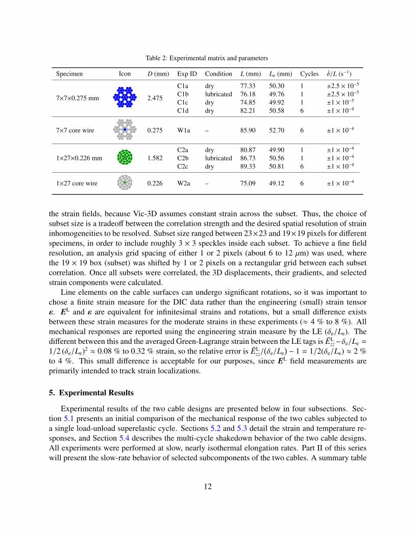
Table 2: Experimental matrix and parameters

Specimen Icon D (mm) Exp ID Condition L (mm) Le (mm) Cycles δ/L (s−1)

7×7×0.275 mm 2.475

C1a dry 77.33 50.30 1 ±2.5 × 10−5

C1b lubricated 76.18 49.76 1 ±2.5 × 10−5

C1c dry 74.85 49.92 1 ±1 × 10−5

C1d dry 82.21 50.58 6 ±1 × 10−4

7×7 core wire 0.275 W1a – 85.90 52.70 6 ±1 × 10−4

1×27×0.226 mm 1.582C2a dry 80.87 49.90 1 ±1 × 10−4

C2b lubricated 86.73 50.56 1 ±1 × 10−4

C2c dry 89.33 50.81 6 ±1 × 10−4

1×27 core wire 0.226 W2a – 75.09 49.12 6 ±1 × 10−4

the strain fields, because Vic-3D assumes constant strain across the subset. Thus, the choice ofsubset size is a tradeoff between the correlation strength and the desired spatial resolution of straininhomogeneities to be resolved. Subset size ranged between 23×23 and 19×19 pixels for differentspecimens, in order to include roughly 3 × 3 speckles inside each subset. To achieve a fine fieldresolution, an analysis grid spacing of either 1 or 2 pixels (about 6 to 12 µm) was used, wherethe 19 × 19 box (subset) was shifted by 1 or 2 pixels on a rectangular grid between each subsetcorrelation. Once all subsets were correlated, the 3D displacements, their gradients, and selectedstrain components were calculated.

Line elements on the cable surfaces can undergo significant rotations, so it was important tochose a finite strain measure for the DIC data rather than the engineering (small) strain tensorε. EL and ε are equivalent for infinitesimal strains and rotations, but a small difference existsbetween these strain measures for the moderate strains in these experiments (≈ 4 % to 8 %). Allmechanical responses are reported using the engineering strain measure by the LE (δe/Le). Thedifferent between this and the averaged Green-Lagrange strain between the LE tags is EL

zz−δe/Le =

1/2 (δe/Le)2 ≈ 0.08 % to 0.32 % strain, so the relative error is ELzz/

(δe/Le

)− 1 = 1/2(δe/Le) ≈ 2 %

to 4 %. This small difference is acceptable for our purposes, since EL field measurements areprimarily intended to track strain localizations.

5. Experimental Results

Experimental results of the two cable designs are presented below in four subsections. Sec-tion 5.1 presents an initial comparison of the mechanical response of the two cables subjected toa single load-unload superelastic cycle. Sections 5.2 and 5.3 detail the strain and temperature re-sponses, and Section 5.4 describes the multi-cycle shakedown behavior of the two cable designs.All experiments were performed at slow, nearly isothermal elongation rates. Part II of this serieswill present the slow-rate behavior of selected subcomponents of the two cables. A summary table

12

of the experiments to be presented here is given in Table 2, showing the various specimens, di-mensions, and experimental parameters. The experiment identifier starts with the type of specimen(C for cable, W for straight wire), then the cable/alloy type (1 for 7×7, 2 for 1×27), and then alowercase letter appended for each experiment performed.

The average axial stress of each specimen is reported as P/A0, where P is the tension forcealong the z-axis and A0 = nπd2/4 is a chosen reference area, based on the number of wires (n)in the specimen and the individual wire diameter (d). Note that this differs somewhat from theprojected cross-sectional area of the wires (normal to the tensile axis), since the cross-section nor-mals of most wires are misaligned to the cable axis. Circular wire cross-sections become projectedapproximately as ellipses3 in the overall cable’s cross-section. Nevertheless, the simple summationof wire cross-sections is a straightforward metric for reporting the macroscopic cable response andfor later comparison with the response of a single straight wire.

The reaction torque, i.e., moment about the z-axis (Mz), generated by constraining the rotationof the specimen at the grips, is reported as MzR/J0, where R is the radius from the center of thespecimen to the outermost point in the cross-section, and J0 is a chosen reference torsion constant.One will recognize τ = MzR/J0 as the classical formula for the maximum shear stress at the outerradius of a linearly elastic, straight, cylindrical rod subjected to twisting about its axis. Our torsionconstant was selected simply as the polar moment of inertia of an idealized (fictitious) cross-sectioncalculated by

J0 = nπd4

32+

n∑i=1

πd2

4r2

i , (1)

where the first term is the contribution of individual wires about their own axes and the second termis the sum of the parallel axis theorem contributions. Here, i is the index of the wire, ri is the meanradius from the central z-axis of the specimen to the wire’s centerline, and wire cross-sections aretreated as circles rather than ellipses. While the elementary theory does not strictly apply here, J0

was chosen for simplicity to give an approximate sense of the average normal stress versus shearstress contributions in the different cable and strand designs.

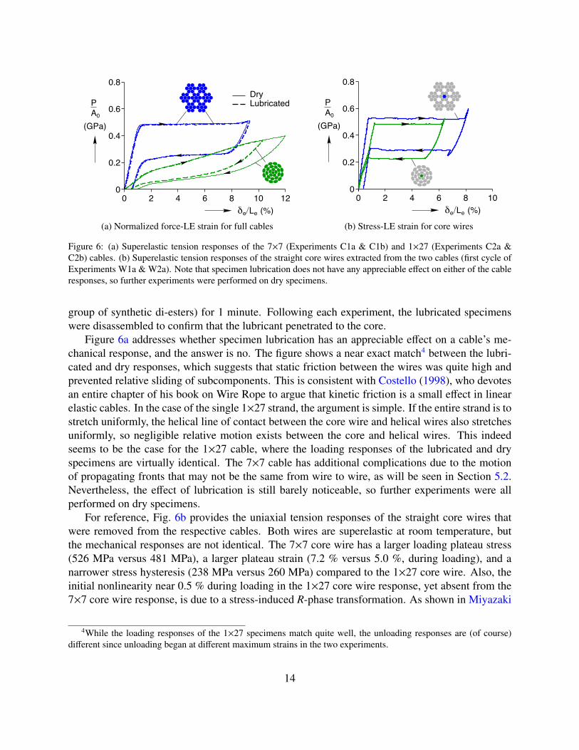
5.1. Initial Comparison of the Two CablesFigure 6a shows the average axial stress versus LE strain of four experiments performed on

the two cable designs. For each cable design one specimen was as-received (dry, solid line) andone was lubricated (dashed line). To have a controlled comparison the cables were not paintedwith speckles for these experiments and thus DIC was not performed. Each pair of dry/lubricatedspecimens was subjected to the same slow rate to avoid thermomechanical coupling effects inroom temperature air (δ/L = ±2.5 × 10−5 s−1 for both 7×7 specimens and δ/L = ±1 × 10−4 s−1

for both 1×27 specimens). Prior to the experiments shown by dashed lines, 7×7 and 1×27 cablespecimens were immersed in penetrating lubricant (Grignard TN-3, composed of a non-petroleum

3The intersection of a helical wire with a plane z =constant is not quite an ellipse due to the wire curvature and itsfinite thickness, especially for tightly wound wires with small spring indices (Ci ≡ ri/rw ' O(1), where ri and rw arethe nominal helix radius and wire cross-section radius, respectively.)

13

0 2 4 6 8 10 120

0.2

0.4

0.6

0.8

LubricatedDry

(GPa)A0

P

δe Le (%)

(a) Normalized force-LE strain for full cables

0 2 4 6 8 100

0.2

0.4

0.6

0.8

(GPa)A0

P

δe Le (%)

(b) Stress-LE strain for core wires

Figure 6: (a) Superelastic tension responses of the 7×7 (Experiments C1a & C1b) and 1×27 (Experiments C2a &C2b) cables. (b) Superelastic tension responses of the straight core wires extracted from the two cables (first cycle ofExperiments W1a & W2a). Note that specimen lubrication does not have any appreciable effect on either of the cableresponses, so further experiments were performed on dry specimens.

group of synthetic di-esters) for 1 minute. Following each experiment, the lubricated specimenswere disassembled to confirm that the lubricant penetrated to the core.

Figure 6a addresses whether specimen lubrication has an appreciable effect on a cable’s me-chanical response, and the answer is no. The figure shows a near exact match4 between the lubri-cated and dry responses, which suggests that static friction between the wires was quite high andprevented relative sliding of subcomponents. This is consistent with Costello (1998), who devotesan entire chapter of his book on Wire Rope to argue that kinetic friction is a small effect in linearelastic cables. In the case of the single 1×27 strand, the argument is simple. If the entire strand is tostretch uniformly, the helical line of contact between the core wire and helical wires also stretchesuniformly, so negligible relative motion exists between the core and helical wires. This indeedseems to be the case for the 1×27 cable, where the loading responses of the lubricated and dryspecimens are virtually identical. The 7×7 cable has additional complications due to the motionof propagating fronts that may not be the same from wire to wire, as will be seen in Section 5.2.Nevertheless, the effect of lubrication is still barely noticeable, so further experiments were allperformed on dry specimens.

For reference, Fig. 6b provides the uniaxial tension responses of the straight core wires thatwere removed from the respective cables. Both wires are superelastic at room temperature, butthe mechanical responses are not identical. The 7×7 core wire has a larger loading plateau stress(526 MPa versus 481 MPa), a larger plateau strain (7.2 % versus 5.0 %, during loading), and anarrower stress hysteresis (238 MPa versus 260 MPa) compared to the 1×27 core wire. Also, theinitial nonlinearity near 0.5 % during loading in the 1×27 core wire response, yet absent from the7×7 core wire response, is due to a stress-induced R-phase transformation. As shown in Miyazaki

4While the loading responses of the 1×27 specimens match quite well, the unloading responses are (of course)different since unloading began at different maximum strains in the two experiments.

14

and Otsuka (1986), certain NiTi alloys exhibit a two stage transformation (A → R+ followed byR+ → M+) when tested 10 to 20 °C above their Af temperature, but the same alloys only show asingle stage transformation (A→ M+) when tested at higher temperatures.

Comparing the dry 7×7 cable response in Fig. 6a to that of its core wire in Fig. 6b, the cableresponse is similar to that of a single superelastic wire in pure tension, since the force has beendivided by the cross sectional area of all 49 wires. It has distinct loading and unloading plateauscommonly found in NiTi wires, which suggest the presence of propagating transformation fronts.Although the cable was strained to δe/Le = 9.3 %, just beyond the loading plateau, most of thisdeformation was recovered with only 0.5 % residual strain remaining after unloading. The tensileload P was 1.42 kN (319 lbf) on the upper plateau. These characteristics should be encouragingfor engineers wishing to leverage the excellent properties of SMA wire into a flexible, compactform that can withstand relatively large forces.

The 1×27 cable response, on the other hand, is significantly different from the typical uniaxialbehavior of its SMA wires. The 1×27 cable response is nonlinear with a slight knee near 2 %strain, but it has no obvious load plateau, i.e., it maintains a positive tangent modulus throughoutloading-unloading. Also, no upturn in tangent modulus is seen, even by the maximum gage strainof δe/Le = 12 %. Here, a reduced axial force and a more compliant behavior has been traded fora larger recovery strain of about 11 %, with a final residual strain of about 1 %. In handling, the1×27 specimen is also quite flexible in bending due to its larger helix angles that avoids directtension/compression along the axis of the individual wires.

Thus, a wide range of cable behaviors can be achieved by simply varying the construction,which represents an opportunity for engineers to tailor the response to match the desired character-istics of specific applications. In particular, the 7×7 design might be desirable where a high initialstiffness is needed, yet distinct load plateaus would be used to mitigate overload conditions or actas a mechanical switch. The 1×27 might be appropriate for applications where a larger recoverablestroke and increased bending compliance are needed and/or a more stable axial response is desired.

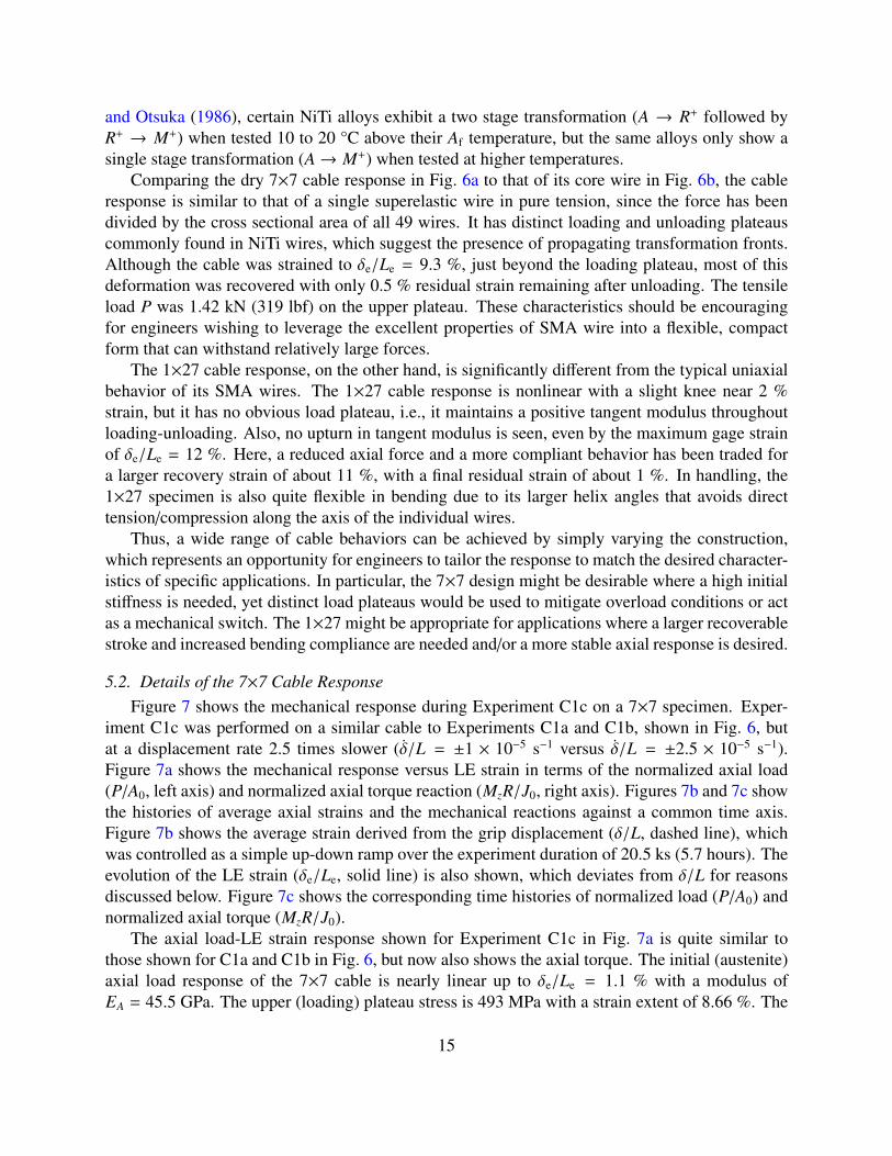
5.2. Details of the 7×7 Cable ResponseFigure 7 shows the mechanical response during Experiment C1c on a 7×7 specimen. Exper-

iment C1c was performed on a similar cable to Experiments C1a and C1b, shown in Fig. 6, butat a displacement rate 2.5 times slower (δ/L = ±1 × 10−5 s−1 versus δ/L = ±2.5 × 10−5 s−1).Figure 7a shows the mechanical response versus LE strain in terms of the normalized axial load(P/A0, left axis) and normalized axial torque reaction (MzR/J0, right axis). Figures 7b and 7c showthe histories of average axial strains and the mechanical reactions against a common time axis.Figure 7b shows the average strain derived from the grip displacement (δ/L, dashed line), whichwas controlled as a simple up-down ramp over the experiment duration of 20.5 ks (5.7 hours). Theevolution of the LE strain (δe/Le, solid line) is also shown, which deviates from δ/L for reasonsdiscussed below. Figure 7c shows the corresponding time histories of normalized load (P/A0) andnormalized axial torque (MzR/J0).

The axial load-LE strain response shown for Experiment C1c in Fig. 7a is quite similar tothose shown for C1a and C1b in Fig. 6, but now also shows the axial torque. The initial (austenite)axial load response of the 7×7 cable is nearly linear up to δe/Le = 1.1 % with a modulus ofEA = 45.5 GPa. The upper (loading) plateau stress is 493 MPa with a strain extent of 8.66 %. The

15

10864200

0.2

0.4

0.6

0.8

M

P

0

0.2

0.1

0.4

0.3

z

(GPa)A0

P

δe Le (%)

(GPa)J0

MzR

(a) Normalized axial force and torque versus LE strain

201510500

5

10

15

L

e Le

z

(%)

(b) Prescribed elongation and LE strain histories

201510500

0.2

0.4

0.6P

(GPa)A0

P

t (ks)

Mz 0.1

0

(GPa)J0

MzR

(c) Normalized axial force and torque histories

Figure 7: Experiment C1c on 7×7 cable at δ/L = ±1 × 10−5 s−1.

lower (unloading) plateau stress is about 262 MPa, but the plateau is flat only between LE strainsof 7.4 % to 5.3 % and the subsequent stress decreases gently until 1.5 % strain, the onset of thefinal linear elastic unload segment.

Interestingly, the torque response in Fig. 7a during loading is non-monotonic. It initially ex-hibits a stiff linear branch with a slope of 13.5 GPa (shear stress/axial strain) up to a maximumtorque at δe/Le = 1.1 %. This is interrupted at the onset of the axial load plateau by a softeningbranch in the torque response. Once the axial load plateau is completed at δe/Le = 8.66 %, thetorque turns upward again slightly. Note that what appears to be a “nucleation peak” in the torqueresponse during loading near δe/Le = 1.1 % is actually an artifact of plotting the response againstδe/Le. As shown in Fig. 7b, the global strain ramps linearly with time, but at the onset of the load-ing plateau the LE strain history is relatively static then suddenly rises more steeply at 4.8 ks. Aswill be shown later, this is due to propagating fronts that first traverse the specimen outside the LEgage section then later enter the LE section. As seen in Fig. 7c, the “nucleation peak” disappearswhen the torque is plotted against the time, and the torque decreases almost linearly during theaxial load plateau. The final residual strain is δ/L = 1.16 % by the grip displacement, but is onlyδe/Le = 0.71 % by the LE measurement. The difference is likely due to some grip slippage that oc-curred during the experiment, a common issue in tension experiments on straight SMA specimens(not dog-bone specimens) that exhibit strain localization. Thus, local extensometer measurementsare a more accurate representation of the material response, even if they can be more difficult tointerpret in the presence of localized strain fields. For this reason, we chose to report δe/Le inFig. 7a instead of δ/L.

The IR temperature and DIC axial strain fields in the 7×7 cable during this experiment are

16

0 5 10 15 200

1

0

0.2

0.4

0.6

0.8

t (ks)

Lz

P

T (oC)19 20 21 22 23

-101

Upper Grip

Ts

LE Tag

LE Tag

1 62 12 1387

DIC

(GPa)A0

P

ΔTs

(°C)

Figure 8: Experiment C1c (7×7 cable at δ/L = ±1 × 10−5 s−1). IR temperature field (contour plot), normalizedforce (overlaid), and specimen thermocouple (above) histories. The labels above the specimen thermocouple historycorrespond to the DIC images in Fig. 9. A scaled schematic of the specimen reference configuration is shown to theleft of the IR temperature plot. The A → M+ transformation appears in the temperature field history as two hot spots(A → M+ fronts) propagating inwards from the grips during loading, but the M+ → A transformation is more diffuseupon unloading, with no clear fronts.

shown in Fig. 8 and Fig. 9, respectively, and both indicate the presence of propagating transfor-mation fronts. The temperature legend in Fig. 8 spans a 4 °C window near room temperature(Ta ≈ 21 °C). The contour plot, T (z, t), was created by taking IR images at 5 s intervals, extract-ing a vertical temperature distribution along the crown of the specimen in each image, stackingthe resulting sequence of one pixel wide slices side-by-side, and synchronizing them with time.Since the laser tags have a much lower emissivity than the painted specimen, they are clearly vis-ible in Fig. 8 as the prominent, but artificial, horizontal streaks. The IR temperature reading isinaccurate there, but the tags do provide good markers for the movement of those locations. Inaddition, the slight horizontal streak in the temperature field history at z/L = 0.46 is due to thespecimen thermocouple. Throughout this paper and Part II, each IR contour plot includes a scaledschematic of the specimen at the left, showing the positions of LE tags and the thermocouplealong the reference specimen length. Disregarding these locations, the overall kinetics of A→ M+

transformation appear as two propagating hot spots, one from each grip, propagating inward andcoalescing at z/L = 0.68 where the temperature reaches as high as 1.5 °C above ambient. Closeinspection reveals that the fronts often appear to propagate in an alternating stop-start fashion, re-sulting in the vertical hot spot streaks in the contour plot. Each time the bottom front moves andheats up, the top front stops and cools down, and vice versa. During unloading, the kinetics ofM+ → A transformation are more diffuse without any clear fronts, just a few scattered local dropsin temperature.

17

Lz

1 2 3 4 5 6 7 8 9 10 11 12 13

0.2

0.4

0.3

Ezz (%)0 2 4 6 8 10

L

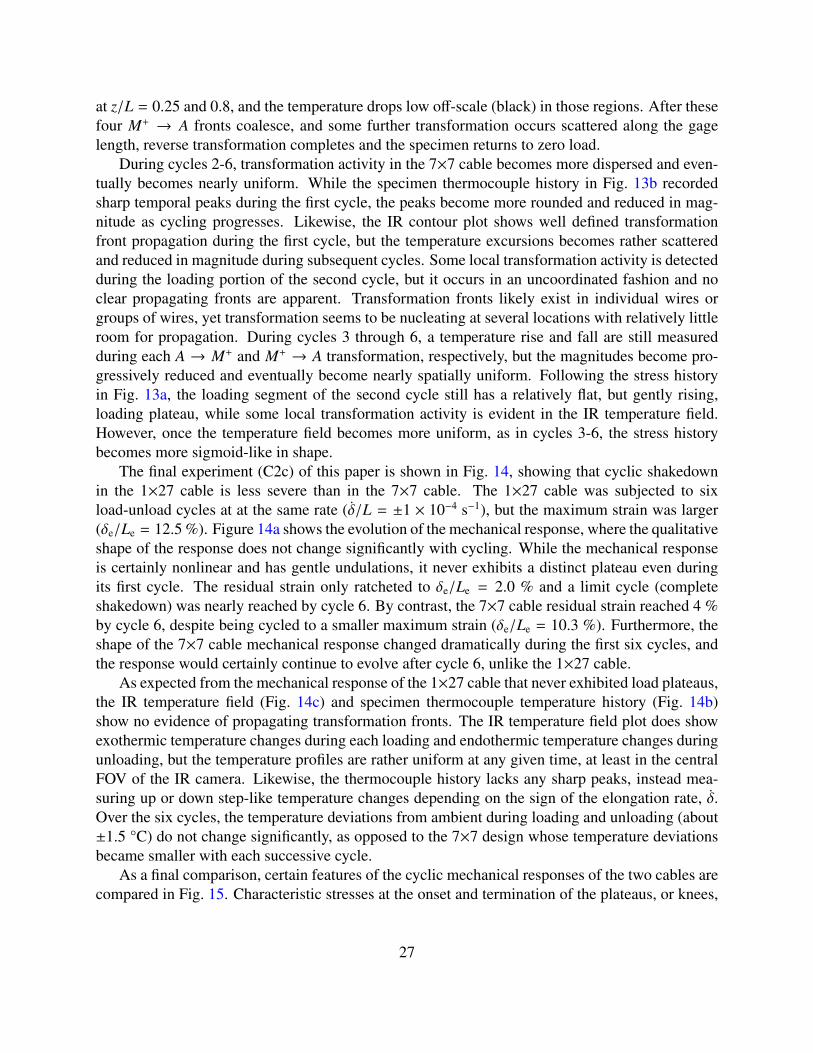
Figure 9: Experiment C1c (7×7 cable at δ/L = ±1×10−5 s−1). DIC axial strain field images which correspond to the labels in Fig. 8. The strain field imagesprovide a magnified view of the front propagation seen in Fig. 8. Note that certain individual wires in the cable do not completely transform as the globalA→ M+ front passes through.

18

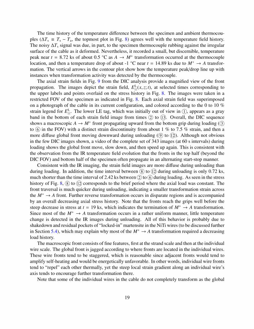
The time history of the temperature difference between the specimen and ambient thermocou-ples (∆Ts ≡ Ts − Ta, the topmost plot in Fig. 8) agrees well with the temperature field history.The noisy ∆Ts signal was due, in part, to the specimen thermocouple rubbing against the irregularsurface of the cable as it deformed. Nevertheless, it recorded a small, but discernible, temperaturepeak near t = 8.72 ks of about 0.5 °C as A → M+ transformation occurred at the thermocouplelocation, and then a temperature drop of about -1 °C near t = 14.89 ks due to M+ → A transfor-mation. The vertical arrows in the contour plot show how the temperature peak/drop line up withinstances when transformation activity was detected by the thermocouple.

The axial strain fields in Fig. 9 from the DIC analysis provide a magnified view of the frontpropagation. The images depict the strain field, EL

zz(x, z; t), at selected times corresponding tothe upper labels and points overlaid on the stress history in Fig. 8. The images were taken in arestricted FOV of the specimen as indicated in Fig. 8. Each axial strain field was superimposedon a photograph of the cable in its current configuration, and colored according to the 0 to 10 %strain legend for EL

zz. The lower LE tag, which was initially out of view in 1 , appears as a grayband in the bottom of each strain field image from times 2 to 13 . Overall, the DIC sequenceshows a macroscopic A → M+ front propagating upward from the bottom grip during loading ( 3to 6 in the FOV) with a distinct strain discontinuity from about 1 % to 7.5 % strain, and then amore diffuse global front moving downward during unloading ( 9 to 12 ). Although not obviousin the few DIC images shown, a video of the complete set of 343 images (at 60 s intervals) duringloading shows the global front move, slow down, and then speed up again. This is consistent withthe observation from the IR temperature field evolution that the fronts in the top half (beyond theDIC FOV) and bottom half of the specimen often propagate in an alternating start-stop manner.

Consistent with the IR imaging, the strain field images are more diffuse during unloading thanduring loading. In addition, the time interval between 8 to 12 during unloading is only 0.72 ks,much shorter than the time interval of 2.42 ks between 2 to 6 during loading. As seen in the stresshistory of Fig. 8, 8 to 12 corresponds to the brief period where the axial load was constant. Thefront traversal is much quicker during unloading, indicating a smaller transformation strain acrossthe M+ → A front. Further reverse transformation occurs in disparate regions and is accompaniedby an overall decreasing axial stress history. Note that the fronts reach the grips well before thesteep decrease in stress at t = 19 ks, which indicates the termination of M+ → A transformation.Since most of the M+ → A transformation occurs in a rather uniform manner, little temperaturechange is detected in the IR images during unloading. All of this behavior is probably due toshakedown and residual pockets of “locked-in” martensite in the NiTi wires (to be discussed furtherin Section 5.4), which may explain why most of the M+ → A transformation required a decreasingload history.

The macroscopic front consists of fine features, first at the strand scale and then at the individualwire scale. The global front is jagged according to where fronts are located in the individual wires.These wire fronts tend to be staggered, which is reasonable since adjacent fronts would tend toamplify self-heating and would be energetically unfavorable. In other words, individual wire frontstend to “repel” each other thermally, yet the steep local strain gradient along an individual wire’saxis tends to encourage further transformation there.

Note that some of the individual wires in the cable do not completely transform as the global

19

0.2

0.3

0.4

1

71113

2

3

4

5

6

10° 20°0°

Lz

φz

Figure 10: Experiment C1c: Profiles of cross-section rotation about the z-axis of the 7×7 cable obtained by DICanalysis. The rotation field is relatively uniform until a global transformation front passes the DIC FOV (images2 - 6 ), at which point the rotation increases substantially and a propagating kink appears.

A → M+ front passes through a given region (see images 2 - 6 ). The likely reason the exteriorwires only partially transform is to maintain axial compatibility with the core strand. As the outersix strands of the cable stretch, they can also reduce their helix angles to accommodate a givenglobal axial strain. The core strand must simply stretch, making the tensile strains in the corewires greater for the same global axial strain. The overall morphology of transformation mustmaintain global axial strain compatibility between the rigid grips, yet high friction between thecomponents within the cable section also tends to enforce local axial strain compatibility betweencomponents. One can imagine that the radial compressive stresses are likely quite large betweenthe outer helical strands and the core strand, since if unsupported the helical strands would contractradially inward (as for a simple tension coil spring taken to large strains). Once the loading plateauis exhausted (t = 10.0 to 10.8 ks), these low strain (austenite) regions shrink slightly (images 6 to7 ). As will be seen in Part II, the end of the core strand plateau corresponds to the upturn in stress

at the end of the 7×7 cable plateau. At this point the outer strands have not yet fully exhausted theirloading plateaus. Only when the core strand begins to uniformly strain again after the terminationof its plateau do the pockets of austenite in the exterior strands begin to disappear.

Another interesting observation is that cable cross-sections rotate about the z-axis. A cablemade of conventional stable material, restrained from rotation at the grips, would not exhibit thisbehavior. Selected cross-section rotation profiles (φz(z), in a right-hand sense) in the DIC FOV areshown in Fig. 10. These were obtained by (1) fitting a cylinder to the DIC data points to determinethe precise location of the z-axis for a cylindrical coordinate system, (2) subtracting the currentangle of each material point from the angle at zero axial load to get φz(θ, z), then (3) averagingacross the cable diameter to obtain an average angle, φz(z), for each cross section. Figure 10 showsthat whenever the strain field is relatively uniform, such as between time t = 0.02 ks ( 1 ) andt = 2.5 ks (just prior to A → M+ transformation) and 7 to 13 (unloading), the cable rotation isrelatively constant along the length and is less than 4o. However, as the macroscopic front traversesthe DIC FOV, 2 to 6 , a kink exists in the rotation profile with a propagating peak (reaching as high

20

121086420

0

0.2

0.4

0

0.2

0.1

P

Mz

(GPa)A0

P

(GPa)J0

MzR

δe Le (%)(a) Normalized axial force and torque versus LE strain

(°C)Ts

101

2.521.510.500

5

10

15

L

e Le

Ts

z

(%)

(b) Prescribed elongation, LE strain, and thermocouple his-tories

P

M

2.521.510.50t (ks)

0

0.2

0.4

0

0.1

0.2z

(GPa)A0

P

(GPa)J0

MzR

(c) Normalized axial force and torque histories

Figure 11: Experiment C2a (1×27 cable at δ/L = ±1 × 10−4 s−1). The torque magnitude in (a) of the 1×27 cable issignificantly larger than that of the 7×7 cable due to the much larger helix angles of the 1×27 wires. Unlike the 7×7cable response, the LE strain in (b) follows the prescribed elongation closely, and the specimen thermocouple recordsstep-like changes in time, both indicating the absence of localized transformation.

as 17.5o in 3 ), whose location corresponds to the position of the global front. Upon subsequentunloading where localized deformation is less prevalent, the rotation at 7 is about 2.3o, and thereis little change between 7 to 11 . After final unloading at 13 the rotation is essentially zero again.

5.3. Details of the 1×27 Cable ResponseWe now turn to Experiment C2a performed on a 1×27 cable specimen at δ/L = ±1 × 10−4 s−1.

The mechanical response is shown in Fig. 11a in terms of the axial load and axial torque versusLE strain. The axial load response is the one shown previously in Fig. 6 (dry).

Relative to its axial load, the torque magnitude of the 1×27 cable is significantly larger than thatof the 7×7 cable. The increase in relative torque magnitude is due to the much larger helix anglesof the 1×27 wires, despite the alternating lays in the construction. The 1×27 torque is negativeaccording to the right-hand sign convention adopted in Fig. 4a, and during loading it exhibits aninteresting multi-step behavior with a knee at about 2 % strain and another knee at about 8 % strain.These undulations will be shown in Part II to be due to transformation activity in the individuallayers of the cross-section occurring at different times.

21

Histories of the average axial strains and specimen thermocouple in Experiment C2a (Fig. 11b)show no evidence of propagating transformation fronts. First, in contrast to the 7×7 cable, the 1×27grip and LE strain histories match more closely. There is a small amount of grip slippage, but theLE strain traces nearly constant-rate ramps. Second, recall that the 7×7 cable specimen thermo-couple measured sharp temperature increases and decreases as the transformation front passed bythe thermocouple (topmost portion of Fig. 8). The 1×27 specimen thermocouple history, on theother hand, indicates a more constant rate of heating/cooling during loading/unloading, withoutany sharp peaks indicative of localized propagating heat sources/sinks.

The specimen thermocouple measurements also suggest that the 1×27 is less rate sensitive.During loading/unloading, the thermocouple measured a rise/drop in temperature of about ±0.5 °C.These deviations from the ambient temperature are roughly the same magnitudes as seen in theprevious experiment on the 7×7 cable, despite the 10× faster elongation rate. The reduced ratesensitivity is due to several factors, including the lack of propagating transformation fronts, thedeeper helix angles in the construction, and the somewhat more slender aspect ratio. A furtherstudy of these factors, as well as experiments at higher rates, can be found in Reedlunn (2011).

5.4. Cyclic Shakedown ResponsesMost SMAs exhibit an evolution of their thermo-mechanical response during their first thermo-

mechanical cycles. This process is called shakedown if the response asymptotically approaches alimit cycle. Since repeatable cyclic behavior is often essential for the success of an SMA device,cyclic shakedown is an important aspect to characterize. In practice, the material may be subjectedto ‘training’ to achieve a repeatable limit-cycle behavior, which additionally may be used to inducea two-way shape memory effect. The degree and cyclic rate of shakedown are strongly dependenton the particular training procedure used and have obvious implications for durability and fatiguelife. Despite intense interest in the literature (e.g. Bo and Lagoudas, 1999; Eggeler et al., 2004;Churchill and Shaw, 2008; Kan and Kang, 2010), a comprehensive map of the influence of possibletraining procedures does not yet exist even for monolithic SMAs, due to the large variety of loadingparameters (temperature, strain, stress) and their path dependence. Accordingly, the purpose of thissection is to preliminarily explore the different cyclic responses of the two cable designs.

Before presenting the cyclic responses of the cables and attempting a comparison, the earlyshakedown responses of the straight core wires extracted from the two cables is shown to establishthe base material differences. The responses to six cycles for each core wire are shown in Fig. 12.The force-elongation responses for the 7×7 and 1×27 core wires are shown respectively in Fig. 12a(Experiment W1a) and Fig. 12c (Experiment W2a), each subjected to six load-unload cycles takento a maximum strain just beyond its load plateau. The corresponding stress and specimen temper-ature histories are shown in Figs. 12b and 12d.

Focussing first on Fig. 12a, the evolution of the superelastic response of the 7×7×0.275 mmcore wire is shown for six cycles to a maximum LE strain of 8.15 %. The cyclic response showshow the superelastic response progresses from one that has distinct plateaus (first cycle, N = 1) toone that has a more sigmoid-like shape (last cycle, N = 6). During this process, the upper plateaumoves downward in stress and the lower plateau moves downward to a lesser degree, until a flatplateau is no longer discernible during either A → M+ or M+ → A. The length of both plateausdecrease and eventually develop a positive tangent modulus, while the strain and temperature fields

22

0 2 4 6 8 100

0.2

0.4

0.6 N = 1 2 3 4 5 6

(GPa)A0

P

δe Le (%)

(a) 7×7 core wire stress-LE strain

0 1 2 3 4 5 6 7 8 9 100

0.2

0.4

0.6 −1

0

1

t (ks)

(°C)ΔTsΔTs

(GPa)A0

P

A0

P

(b) 7×7 core wire stress and thermocouple histories

0 2 4 6 80

0.2

0.4

0.6N = 1 2 3 4 5 6

(GPa)A0

P

δe Le (%)

(c) 1×27 core wire stress-LE strain

0 1 2 3 4 5 6 7 8 9 10 110

0.2

0.4

0.6

−1

0

1

2

(°C)ΔTs

ΔTs

t (ks)

(GPa)A0

P

A0

P

(d) 1×27 core wire stress and thermocouple histories

Figure 12: Superelastic cyclic responses at δ/L = ±1 × 10−4 s−1 (Experiments W1a and W2a) of the straight core wires extracted from the two cables. The1×27 core wire stress-strain response in (a) shows less severe shakedown than the 7×7 core wire in (c). Furthermore, unlike the 7×7 core wire in (b), the1×27 core wire temperature history in (d) shows temporal spikes in the specimen temperature for all six cycles. These spikes, and the flat stress plateaus in(c), indicate persistent R+ ↔ M+ transformation fronts in the 1×27 core wire during cycling.

23

tend to become more uniform (although not shown here). As cycling proceeds, the magnitude ofthe hysteresis (area within the loop) diminishes. The residual strain, upon each unloading to zeroaxial load, evolves forward in strain (ratchets) with progressively smaller increments after cycle 2.Interestingly, the increment of residual strain accumulation after cycle 2 is actually larger than aftercycle 1, but decreases monotonically thereafter. The final residual strain after cycle 6 is 2.74 %.This is only one specific example, relevant to the study at hand, and more cycles would be requiredto truly reach a limit cycle behavior.

The specimen thermocouple history of the 7×7 core wire in Fig. 12b indicates the transitionfrom distinct transformation fronts toward spatially diffuse transformations. Figure 12b showsboth the specimen temperature changes, as measured by a thermocouple placed near the bottomlaser tag, and the axial stress history for reference. The temperature excursions are about ±0.6 °Cduring cycles 1 and 2 and are relatively sharp in time (≈ 150 s duration), indicating localized trans-formation as transformation fronts pass the thermocouple location. A final sharp peak is measuredduring cycle 4 at 6 ks, which is due to a new nucleation event. Subsequently, however, the temper-ature changes become progressively rounded and diminished in magnitude to roughly ±0.1 °C bycycle 6, indicating more diffuse transformations. As expected, this change in temperature behaviorcorresponds to the disappearance of the stress plateaus.

In contrast to the 7×7 core wire, Fig. 12c shows a less severe shakedown in the mechanicalresponse of the 1×27 core wire. The stress plateaus remain over the six cycles but just shift down-ward somewhat in each cycle (about −35 MPa in total). The residual strain even after cycle 6 isonly 0.1 %, and the superelastic loop remains nearly closed. Figure 12d shows that, unlike the 7×7core wire, the temporal spikes in specimen temperature exist for all six cycles. Both this featureand the flatness of the stress plateaus indicate that phase transformations still involve propagatingfronts.

Clearly the alloys are not identical, which is unfortunate for a direct comparison between thetwo cables. We suspect processing variables for the two cable constructions were varied, leadingto the different material properties. As shown in the DSC thermograms of Fig. 3, we estimate thatthe 1×27 wire is superelastic above 10 °C, while the 7×7 wire is superelastic above -24 °C. Thisdifference causes the 1×27 wire to have a −45 MPa lower loading plateau stress and a −64 MPalower unloading plateau stress in the first cycle. Because the plateau strain is also smaller for the1×27 wire, the maximum strain during cycling was less (6.41 % vs. 8.19 %). Generally speaking,the cyclic rate of shakedown (if ever reached) is quite sensitive to the transformation stress, andthus to the specimen temperature according to the Clausius-Clapeyron relation. The shakedownevolution is also indirectly sensitive to the maximum strain, especially if taken well beyond theinitial loading plateau. Had we taken the 1×27 wire to the same maximum strain as the 7×7 wire,which would have been well into the post-plateau regime, the shakedown would have been moresevere.

The mechanical response of the full 7×7 cable (Exp. C1d) during cycling (Fig. 13a) is qualita-tively similar to that of its core wire (Fig. 12a). To reduce the duration of this longer experiment(Exp. C1d) the elongation rate was δ/L = ±1 × 10−4 s−1, ten times faster than the previous 7×7cable experiment (C1c). This rate is still rather slow, however, and is the same rate used in thecyclic core wire experiment (Exp. W1a). The maximum strain during each cycle on the 7×7 cable

24

was δe/Le = 10.37 %, just beyond the initial load plateau as shown in Fig. 13a. In the first cycleof the 7×7 cable, after the initial stiff, nearly linear, mechanical response, there exist the usualdistinct plateaus during loading (A → M+ transformation) and unloading (M+ → A transforma-tion). The subsequent cycles exhibit the typical superelastic shakedown response for NiTi whenstress-induced transformation requires a large stress (over 500 MPa in this case). Similar to thecore wire response, the mechanical response becomes more sigmoid-like as cycling proceeds, andthe magnitude of the hysteresis (area within the loop) diminishes. At the same time, the strain atzero stress increases, but in successively smaller increments for each cycle (again after cycle 2).Comparing cycle 1 and 6 of the 7×7 cable, the incremental changes with cycles are qualitativelysimilar to that of the core wire (Fig. 12a), but the changes are larger for the cable specimen.

The cyclic evolution of the 7×7 cable specimen thermocouple readings follow the same generaltrend shown for its core wire in Fig. 12b, but quantitative differences do exist. First, the temperaturepeaks during the first cycle occur over about 1000 s, indicating that transformation in the cable ismore diffuse than in the core wire. Second, the magnitudes of the temperature excursion are largerin the cable for the same global strain rate (note the different temperature scales). In cycle 1, thetemperature excursions are ±2.5 °C, which fades to ±1.4 °C by cycle 6. This larger temperaturechange is due to the larger thermal scaling (volume/exposed surface area ratio) of the cable, despitethe more diffuse transformation in the cable compared to the wire.

The 7×7 cable IR contour plot (Fig. 13c) clearly shows localized transformation front activityduring the first cycle. The FOV of the IR camera in this experiment includes most, but not all, of thefree length, and the color legend spans 6 °C about ambient room temperature (20 °C). During thefirst cycle, as expected from the flat loading and unloading plateaus, the temperature field showstransformation fronts traversing the specimen gage length (again ignore the LE tag locations). Onefront nucleates at the top grip and another front nucleates at the bottom grip, due to the stressconcentrations there. Once the temperature of the initial two fronts rises by about 2.2 °C, anotherpair of fronts nucleate at z/L = 0.7. The top two fronts, one from the top grip, the other fromthe z/L = 0.7 nucleation, coalesce at z/L = 0.8, at which point a very small drop in the loadwas measured at t = 0.85 ks. This leaves only the bottom two fronts, which speed up to complywith the global strain rate δ/L = ±1 × 10−4 s−1, thereby raising the local exothermic heat releaserate. As these fronts propagate and approach each other, they thermally interact, locally raising thetemperature to 24.7 °C, above the limit of the temperature scale in the figure, when they coalesce atz/L = 0.4. The temperature rise is accompanied by a 22 MPa increase in propagation stress. Afterthe fronts coalesce, the specimen temperature does not immediately return to room temperature(cyan). Instead, the specimen remains above ambient by about 1 °C. In fact, the upper edge of theIR FOV that had briefly cooled to room temperature, heats up again when the axial load takes itsupturn after the plateau. During this time, a vertical green band is observed across the entire FOV,which is likely due to the regions of austenite shown in images 3 - 7 of Fig. 9, which were leftbehind by the global front, finally transforming to martensite. We do not have DIC data for thisexperiment to prove the point, but given that the uniform heating occurs between δe/Le = 8.8 %and 10.2 %, and the remnant regions of austenite started to transform at δe/Le = 8.7 % in theisothermal DIC experiment, we are confident this is the case. During the unloading plateau, twofronts emanate from the final coalescent site during loading, and close inspection reveals evidence

25

0 2 4 6 8 10 120

0.2

0.4

0.6 N = 1 2 3 4 5 6

(GPa)A0

P

δe Le (%)

(a) Normalized force-LE strain

0 1 2 3 4 5 6 7 8 9 10 114

4

0

ΔTs

(°C)

(b) Specimen thermocouple history

N = 1 2 3 4 5 6

0 1 2 3 4 5 6 7 8 9 10 110

1

0

0.2

0.4

0.6

0.8

t (ks)

P

T(oC)17 18 19 20 21 22 23

Ts

LE Tag

LE Tag

(GPa)A0

PLz

(c) IR temperature field (contour plot) and normalized force (overlaid) histories

Figure 13: Experiment C1d (6 cycles of a 7×7 specimen at δ/L = ±1× 10−4 s−1). Consistent with the cyclic evolutionof the mechanical response in (a), well-defined transformation fronts are clearly visible only during the first cyclein (c), with transformations exhibiting progressively more uniform temperature profiles during subsequent cycling.Compared to its core wire (Fig. 12b), the full cable’s temperature response shows larger temperature excursions (dueto the larger thermal scaling) and more diffuse transformations, both spatially and temporally.

of transformation activity near the other coalescent site as well (cool spots near z/L = 0.75 att = 1.6 ks). Reverse nucleations at the site of A→ M+ front coalescences are commonly observedin uniaxially loaded wires (Chang et al., 2006), so the observation here is not surprising. The twoM+ → A fronts from z/L = 0.4 propagate outward until they meet fronts emanating from the grips

26

at z/L = 0.25 and 0.8, and the temperature drops low off-scale (black) in those regions. After thesefour M+ → A fronts coalesce, and some further transformation occurs scattered along the gagelength, reverse transformation completes and the specimen returns to zero load.

During cycles 2-6, transformation activity in the 7×7 cable becomes more dispersed and even-tually becomes nearly uniform. While the specimen thermocouple history in Fig. 13b recordedsharp temporal peaks during the first cycle, the peaks become more rounded and reduced in mag-nitude as cycling progresses. Likewise, the IR contour plot shows well defined transformationfront propagation during the first cycle, but the temperature excursions becomes rather scatteredand reduced in magnitude during subsequent cycles. Some local transformation activity is detectedduring the loading portion of the second cycle, but it occurs in an uncoordinated fashion and noclear propagating fronts are apparent. Transformation fronts likely exist in individual wires orgroups of wires, yet transformation seems to be nucleating at several locations with relatively littleroom for propagation. During cycles 3 through 6, a temperature rise and fall are still measuredduring each A → M+ and M+ → A transformation, respectively, but the magnitudes become pro-gressively reduced and eventually become nearly spatially uniform. Following the stress historyin Fig. 13a, the loading segment of the second cycle still has a relatively flat, but gently rising,loading plateau, while some local transformation activity is evident in the IR temperature field.However, once the temperature field becomes more uniform, as in cycles 3-6, the stress historybecomes more sigmoid-like in shape.

The final experiment (C2c) of this paper is shown in Fig. 14, showing that cyclic shakedownin the 1×27 cable is less severe than in the 7×7 cable. The 1×27 cable was subjected to sixload-unload cycles at at the same rate (δ/L = ±1 × 10−4 s−1), but the maximum strain was larger(δe/Le = 12.5 %). Figure 14a shows the evolution of the mechanical response, where the qualitativeshape of the response does not change significantly with cycling. While the mechanical responseis certainly nonlinear and has gentle undulations, it never exhibits a distinct plateau even duringits first cycle. The residual strain only ratcheted to δe/Le = 2.0 % and a limit cycle (completeshakedown) was nearly reached by cycle 6. By contrast, the 7×7 cable residual strain reached 4 %by cycle 6, despite being cycled to a smaller maximum strain (δe/Le = 10.3 %). Furthermore, theshape of the 7×7 cable mechanical response changed dramatically during the first six cycles, andthe response would certainly continue to evolve after cycle 6, unlike the 1×27 cable.

As expected from the mechanical response of the 1×27 cable that never exhibited load plateaus,the IR temperature field (Fig. 14c) and specimen thermocouple temperature history (Fig. 14b)show no evidence of propagating transformation fronts. The IR temperature field plot does showexothermic temperature changes during each loading and endothermic temperature changes duringunloading, but the temperature profiles are rather uniform at any given time, at least in the centralFOV of the IR camera. Likewise, the thermocouple history lacks any sharp peaks, instead mea-suring up or down step-like temperature changes depending on the sign of the elongation rate, δ.Over the six cycles, the temperature deviations from ambient during loading and unloading (about±1.5 °C) do not change significantly, as opposed to the 7×7 design whose temperature deviationsbecame smaller with each successive cycle.

As a final comparison, certain features of the cyclic mechanical responses of the two cables arecompared in Fig. 15. Characteristic stresses at the onset and termination of the plateaus, or knees,

27

0 2 4 6 8 10 12 140

0.2

0.4

0.6

N = 1 2 3 4 5 6(GPa)A0

P

δe Le (%)

(a) Normalized force-LE strain

0 1 2 3 42

0

2ΔTs

(°C)

(b) Specimen thermocouple history

0 1 2 3 40

1

0

0.2

0.4

0.6

t (ks)

P

T(oC)T(oC)18 19 20 21 22 23 2418 19 20 21 22 23 24

N = 1 2 3 4 5 6

Ts

LE Tag

LE Tag

(GPa)A0

PLz

(c) IR temperature field (contour plot) and normalized force (overlaid) histories

Figure 14: Experiment C2c (six cycles of a 1×27 cable at δ/L = ±4 × 10−4 s−1). The 1×27 cable response exhibitsrelatively mild shakedown in (a), and the uniform temperature fields in (c) at each time instant confirm the absence ofpropagating transformation fronts.

in the response curves are shown in Fig. 15a and 15b for the respective cables. The insets in thefigures show the constructions used to extract these stresses from the mechanical response (finalcycle response shown) in a systematic way. For the 7×7 cable, Fig. 15a shows that stresses at theonset/termination of the A → M+ plateau generally decrease with cycles, but diverge from eachother as the response curve becomes more sigmoid-like. The stresses during the M+ → A plateau

28

0

0.2

0.4

0.6

0.8

654321N

(GPa)σ*

N = 6

1086420δe Le (%)

128

(a) A↔ M+ stresses versus cycles (7×7)

0

0.2

0.4

0.6

0.8

(GPa)σ*

654321N

δe Le (%)

N = 6

14121086420

(b) R+ ↔ M+ stresses versus cycles (1×27)

654321N

0

1

2

3

4

(%)εr

(c) Residual strains versus cycles

6543210

20

40

60

80

N

�GPa�E Loading

Unloading

(d) Initial and final moduli versus cycles

Figure 15: Comparison of the cyclic evolution of 7×7 and 1×27 cable responses, showing (a,b) characteristic trans-formation stresses, (c) residual strains, and (d) initial loading modulus (closed symbols) and unloading modulus (opensymbols). These again show a more dramatic cyclic evolution of response features in the 7×7 cable than in the1×27cable.

also diverge from each other, but the onset of the knee moves upward in stress while the reverseknee near the termination of M+ → A transformation moves downward. The average of thesetwo values remains relatively constant with cycling. The cyclic trends in each value are relativelymonotonic, and the dotted lines are single-exponential fits of the data (for N ≥ 2) as discussedfurther below. The trends in the characteristic stresses for the 1×27 cable in Fig. 15b are lessdramatic. The first knee in the curve, which indicates the onset of transformation to M+, quicklyconverges to an asymptotic value by about cycle 3. The other three characteristic stresses changevery little over the six cycles.

Figure 15c plots the residual strains upon complete unloading after each cycle, and Fig. 15dplots the initial and final elastic moduli for each cycle. The dashed lines are exponential fits thatnicely capture the trends of the data, at least for these few cycles. For example, we chose theform εr(N) = ε∞r

[1 − exp

(−

N−N0τ

)]for the residual strain fits. Figure 15c clearly shows the more

extreme evolution of the residual strain for the 7×7 cable with a predicted asymptotic value of

29

about 4.3 % strain, compared to the 1×27 cable which has a predicted asymptotic value of about2.3 % strain. Interestingly, the data fits in Fig. 15c do not extrapolate to the origin as one mightexpect, again showing that the first cycle is somewhat of an outlier in the overall cyclic trends inthe mechanical response (as it was for the straight wire). Likewise, the trends in Fig. 15d show asignificantly reduced elastic modulus for the 7×7 cable, but very little change in elastic modulusfor the 1×27 cable.

The exponential-like behavior (starting with the second cycle) in all these features suggeststhat their evolution may be governed by a Maxwellian “rate” equation. For example, suppose thecharacteristic stresses are each governed by the first-order differential equation

dσdN

= −σ

τ, (2)

where τ is a “time-constant” in terms of the number of full transformation cycles the materialexperiences. This has the exponential solution

∆σ(N) = ∆σ∞

[1 − exp

(−

Nτ

)], (3)

where ∆σ(N) is the change in the transformation stress from its initial value, and ∆σ∞ is theasymptotic (shaken down) change after a sufficiently large number of cycles. We suspect the cyclic“rate-constant” (τ) during shakedown is determined more by the material and the temperature atwhich the experiment was run, than by the construction of the cable. The amount of shakedown(∆σ∞), however, is probably a strong function of the cable construction, since it influences thedistribution and multi-axiality of the local stress state in the wires.

Of course, the maximum strains between the two experiments are different, so a direct com-parison here is difficult. Furthermore, as shown previously in Fig. 12, the two cable designs wereconstructed from somewhat different NiTi alloys so it is not possible to quantitatively determinehow much of the difference in shakedown behavior is due to the cable design versus differences inmaterial properties. We leave for later the challenging modeling task of determining shakedownin various cable constructions from the underlying cyclic constitutive behavior of its individualwires. Nevertheless, given the enhanced compliance of the 1×27 components and lack of propagat-ing transformation fronts (in all but perhaps the single core wire), the cable construction certainlyplays a significant role.

Overall, the data suggests the 1×27 cable may have better ultimate fatigue performance, dura-bility, and overall high-cycle repeatability. Of course, this comes at the cost of a significantlyreduced stiffness and less dramatic transitions between elastic and phase transformation regions,if those are desired. Thus, the question of which cable design is favored depends on the intendedapplication. It should be apparent by now that many other possible constructions could be investi-gated to obtain behaviors in between, or drastically different, from those shown here.

6. Summary & Conclusions

The room temperature, nearly isothermal tensile responses of the 7×7×0.275 mm cable and1×27×0.226 mm cable were characterized. Both cable design responses were relatively unaffected

30

by lubrication, indicating high friction between the subcomponents. Overall, the mechanical re-sponses of the 7×7 cable and the straight core wire extracted from it were quite similar, indicatingthe 7×7 cable behaves similar to that of 49 straight wires loaded in parallel. The behavior of the1×27 cable was considerably different due to the larger helix angles involved in its construction.Thus, the 7×7 cable may be ideal for those engineers wishing to exploit the excellent propertiesof superelastic wires in a high force, compact package, while the 1×27 cable trades off force fora larger recoverable strain, exhibits a more stable structural response with a positive tangent mod-ulus, and less severe shakedown characteristics. Both cables had an interesting non-monotonictorque reaction during the tension experiments, yet the relative magnitude was more significant inthe 1×27 cable due to the larger helix angles in its construction.

Simultaneous infrared thermography and stereo digital image correlation were used during theexperiments on the two designs to investigate the local strain and temperature field variations.The 7×7 cable clearly exhibited propagating phase transformation fronts that behaved in a similarmanner to the fronts in its straight core wire. Some interesting features were observed, however,in the propagation of fronts between adjacent wires in the cable and some incomplete propagationin some of the outermost wires. Stress-induced phase transformation activity was detected in thetemperature fields of the 1×27, but no propagating transformation fronts were observed. This madethe 1×27 specimen less sensitive to latent heat-induced temperature changes, allowing relativelyisothermal experiments to be performed at faster elongation rates than for the 7×7 cable. The rangeof responses for the two cable designs seems to indicate significant future opportunities to tailorthe structural behavior of SMA cables to their intended applications by designing the constructionand layups.

Part II that follows will study the response of selected subcomponents excised from the twocable constructions to asses the individual contributions of the cables’ hierarchical construction.

AcknowledgementsWe gratefully acknowledge the financial support for this work, provided by General Motors

Research and Development through the GM/UM Collaborative Research Laboratory (CRL) inSmart Materials and Structures, the National Science Foundation (CMMI-0727331), and the USDepartment of Energy, Office of Basic Energy Sciences (DE-SC0003996). Helpful discussionswith the members of the GM/UM CRL throughout the course of this work are acknowledged.Specimen materials were provided by Fort Wayne Metals Research at no cost, along with helpfulguidance, which are also very much appreciated.

References

Barooah, P., Rey, N., 2002. Closed-loop control of a shape memory alloy actuation system for variable areafan nozzle, in: Rao, V.S. (Ed.), Proceedings of SPIE, pp. 384–395.

Bo, Z., Lagoudas, D., 1999. Thermomechanical modeling of polycrystalline SMAs under cyclic loading,Part III: evolution of plastic strains and two-way shape memory effect. International Journal of Engineer-ing Science 37, 1175–1203.

31

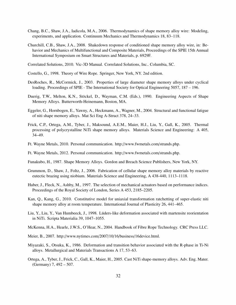
Chang, B.C., Shaw, J.A., Iadicola, M.A., 2006. Thermodynamics of shape memory alloy wire: Modeling,experiments, and application. Continuum Mechanics and Thermodynamics 18, 83–118.

Churchill, C.B., Shaw, J.A., 2008. Shakedown response of conditioned shape memory alloy wire, in: Be-havior and Mechanics of Multifunctional and Composite Materials, Proceedings of the SPIE 15th AnnualInternational Symposium on Smart Structures and Materials, p. 6929F.

Correlated Solutions, 2010. Vic-3D Manual. Correlated Solutions, Inc.. Columbia, SC.

Costello, G., 1998. Theory of Wire Rope. Springer, New York, NY. 2nd edition.

DesRoches, R., McCormick, J., 2003. Properties of large diameter shape memory alloys under cyclicalloading. Proceedings of SPIE - The International Society for Optical Engineering 5057, 187 – 196.

Duerig, T.W., Melton, K.N., Stockel, D., Wayman, C.M. (Eds.), 1990. Engineering Aspects of ShapeMemory Alloys. Butterworth-Heinemann, Boston, MA.

Eggeler, G., Hornbogen, E., Yawny, A., Heckmann, A., Wagner, M., 2004. Structural and functional fatigueof niti shape memory alloys. Mat Sci Eng A-Struct 378, 24–33.

Frick, C.P., Ortega, A.M., Tyber, J., Maksound, A.E.M., Maier, H.J., Liu, Y., Gall, K., 2005. Thermalprocessing of polycrystalline NiTi shape memory alloys. Materials Science and Engineering: A 405,34–49.

Ft. Wayne Metals, 2010. Personal communication. http://www.fwmetals.com/strands.php.

Ft. Wayne Metals, 2012. Personal communication. http://www.fwmetals.com/strands.php.

Funakubo, H., 1987. Shape Memory Alloys. Gordon and Breach Science Publishers, New York, NY.

Grummon, D., Shaw, J., Foltz, J., 2006. Fabrication of cellular shape memory alloy materials by reactiveeutectic brazing using niobium. Materials Science and Engineering, A 438-440, 1113–1118.

Huber, J., Fleck, N., Ashby, M., 1997. The selection of mechanical actuators based on performance indices.Proceedings of the Royal Society of London, Series A 453, 2185–2205.

Kan, Q., Kang, G., 2010. Constitutive model for uniaxial transformation ratchetting of super-elastic nitishape memory alloy at room temperature. International Journal of Plasticity 26, 441–465.

Liu, Y., Liu, Y., Van Humbeeck, J., 1998. Luders-like deformation associated with martensite reorientationin NiTi. Scripta Materialia 39, 1047–1055.

McKenna, H.A., Hearle, J.W.S., O’Hear, N., 2004. Handbook of Fibre Rope Technology. CRC Press LLC.

Meier, B., 2007. http://www.nytimes.com/2007/10/16/business/16device.html.

Miyazaki, S., Otsuka, K., 1986. Deformation and transition behavior associated with the R-phase in Ti-Nialloys. Metallurgical and Materials Transactions A 17, 53–63.

Ortega, A., Tyber, J., Frick, C., Gall, K., Maier, H., 2005. Cast NiTi shape-memory alloys. Adv. Eng. Mater.(Germany) 7, 492 – 507.

32

Otsuka, K., Sawamura, T., Shimizu, K., 1971. Crystal structure and internal defects of equiatomic TiNimartensite. Phys. State. Sol. (A) 5, 457.

Otsuka, K., Wayman, C.M., 1998. Shape Memory Materials. Cambridge University Press, Cambridge, UK.

Redmond, J.A., Brei, D., Luntz, J., Browne, A.L., Johnson, N.L., 2008. Behavioral model and experimentalvalidation for a spool-packaged shape memory alloy actuator, in: Davis, L.P., Henderson, B.K., McMick-ell, M.B. (Eds.), In: Proceedings of SPIE, Industrial and Commercial Applications of Smart StructuresTechnologies 2008, SPIE. pp. 693004–69004–13.

Reedlunn, B., 2011. Thermomechanical Behavior of Shape Memory Alloy Cables and Tubes. PhD disser-tation. The University of Michigan. Department of Mechanical Engineering.

Reedlunn, B., Daly, S., Hector, L.G.J., Zavattieri, P., Shaw, J.A., 2013. Tips and tricks for characterizingshape memory alloy wire: Part 5 – full-field strain measurement by digital image correlation. Experi-mental Techniques 37, 62–78.

Reedlunn, B., Shaw, J., Daly, S., 2010. Pseudoelastic shape memory alloy cables, in: Grummon, D.S.,Mitchell, M.R., Mertmann, M. (Eds.), Proceedings of the International Conference on Shape Memoryand Superelastic Technologies (SMST 2010), ASM. Springer.

Reedlunn, B., Shaw, J.A., 2008. Shape memory alloy cables, in: Dapino, M.J., Ounaies, Z. (Eds.), Pro-ceedings of the SPIE 15th Annual International Symposium in Smart Structures and Materials, SPIE. p.69291G.

Reedlunn, B., Shaw, J.A., Daly, S., 2009. Shape memory alloy cables: Exploratory experiments, in: Pro-ceedings of the ASME Conference on Smart Materials, Adaptive Structures and Intelligent Systems(SMASIS 2009), ASME. pp. 149–160.

Rey, N.M., Tillman, G., Miller, R.M., Wynosky, T., Larkin, M.J., Flamm, J.D., Bangert, L.S., 2001. Shapememory alloy actuation for a variable area fan nozzle, in: A.-M. R. McGowan (Ed.), Society of Photo-Optical Instrumentation Engineers (SPIE) Conference Series, pp. 371–382.

Semba, H., Okabe, N., Yamaji, T., Okita, K., Yamauchi, K., 2005. Axial compressive behavior of single-stage bellows of TiNi shape memory alloy for seismic applications. Materials Science Forum 475-479,2055–2058.

Shaw, J.A., Churchill, C.B., Iadicola, M.A., 2008. Tips and tricks for characterizing shape memory alloywire: Part 1 – differential scanning calorimetry & basic phenomena. Experimental Techniques , 55–62.

Shaw, J.A., Grummon, D.S., Foltz, J., 2007. Superelastic NiTi honeycombs: Fabrication and experiments.Smart Materials and Structures 16, S170–S178.

Shaw, J.A., Kyriakides, S., 1995. Thermomechanical aspects of NiTi. Journal of the Mechanics and Physicsof Solids 43, 1243–1281.

Shaw, J.A., Kyriakides, S., 1997. On the nucleation and propagation of phase transformation fronts in aNiTi alloy. Acta Materialia 45, 683–700.

33

Shaw, J.A., Kyriakides, S., 1998. Initiation and propagation of localized deformation in elasto–plastic stripsunder uniaxial tension. International Journal of Plasticity 13, 837–871.

Song, G., Mo, Y.L., Otero, K., Gu, H., 2006. Health monitoring and rehabilatation of a concrete structureusing intelligent materials. Smart Materials and Structures 15, 309–314.

Sun, Q.P., Li, Z.Q., Tse, K.K., 2000. On superelastic deformation of NiTi shape memory alloy micro–tubesand wires — band nucleation and propagation. Proceedings of IUTAM Symposium on Smart Structuresand Structronic Systems, Magdeburg Germany .

Sutton, M.A., Orteu, J.J., Schreier, H.W., 2009. Image Correlation for Shape, Motion, and DeformationMeasurements: Basic Concepts, Theory, and Applications. Springer, New York.

34