KUNS-1716

hep-th/0104130

Superconformal Tensor Calculus

in Five Dimensions

Tomoyuki Fujita∗) and Keisuke Ohashi∗∗)

Department of Physics, Kyoto University, Kyoto 606-8502, Japan

Abstract

We present a full superconformal tensor calculus in five spacetime dimensions in

which the Weyl multiplet has 32 Bose plus 32 Fermi degrees of freedom. It is derived

using dimensional reduction from the 6D superconformal tensor calculus. We present

two types of 32+32 Weyl multiplets, a vector multiplet, linear multiplet, hypermultiplet

and nonlinear multiplet. Their superconformal transformation laws and the embedding

and invariant action formulas are given.

∗) E-mail: fujita@gauge.scphys.kyoto-u.ac.jp∗∗) E-mail: keisuke@gauge.scphys.kyoto-u.ac.jp

1 typeset using PTPTEX.sty <ver.1.0>

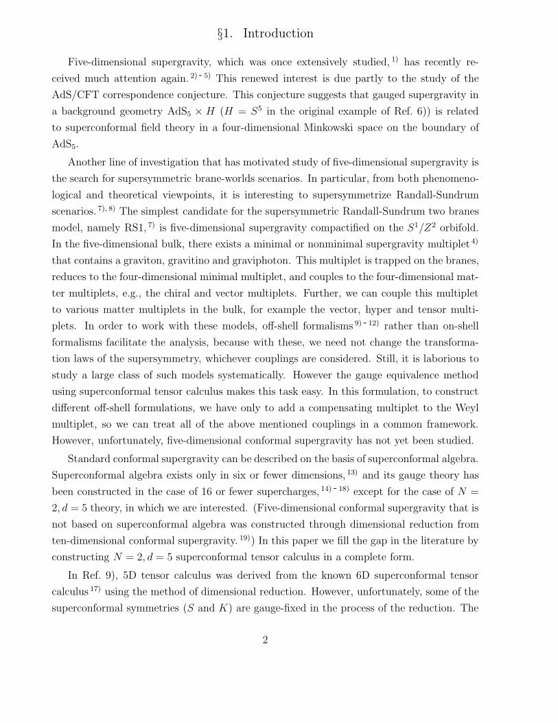
§1. Introduction

Five-dimensional supergravity, which was once extensively studied, 1) has recently re-

ceived much attention again. 2) - 5) This renewed interest is due partly to the study of the

AdS/CFT correspondence conjecture. This conjecture suggests that gauged supergravity in

a background geometry AdS5 × H (H = S5 in the original example of Ref. 6)) is related

to superconformal field theory in a four-dimensional Minkowski space on the boundary of

AdS5.

Another line of investigation that has motivated study of five-dimensional supergravity is

the search for supersymmetric brane-worlds scenarios. In particular, from both phenomeno-

logical and theoretical viewpoints, it is interesting to supersymmetrize Randall-Sundrum

scenarios. 7), 8) The simplest candidate for the supersymmetric Randall-Sundrum two branes

model, namely RS1, 7) is five-dimensional supergravity compactified on the S1/Z2 orbifold.

In the five-dimensional bulk, there exists a minimal or nonminimal supergravity multiplet 4)

that contains a graviton, gravitino and graviphoton. This multiplet is trapped on the branes,

reduces to the four-dimensional minimal multiplet, and couples to the four-dimensional mat-

ter multiplets, e.g., the chiral and vector multiplets. Further, we can couple this multiplet

to various matter multiplets in the bulk, for example the vector, hyper and tensor multi-

plets. In order to work with these models, off-shell formalisms 9) - 12) rather than on-shell

formalisms facilitate the analysis, because with these, we need not change the transforma-

tion laws of the supersymmetry, whichever couplings are considered. Still, it is laborious to

study a large class of such models systematically. However the gauge equivalence method

using superconformal tensor calculus makes this task easy. In this formulation, to construct

different off-shell formulations, we have only to add a compensating multiplet to the Weyl

multiplet, so we can treat all of the above mentioned couplings in a common framework.

However, unfortunately, five-dimensional conformal supergravity has not yet been studied.

Standard conformal supergravity can be described on the basis of superconformal algebra.

Superconformal algebra exists only in six or fewer dimensions, 13) and its gauge theory has

been constructed in the case of 16 or fewer supercharges, 14) - 18) except for the case of N =

2, d = 5 theory, in which we are interested. (Five-dimensional conformal supergravity that is

not based on superconformal algebra was constructed through dimensional reduction from

ten-dimensional conformal supergravity. 19)) In this paper we fill the gap in the literature by

constructing N = 2, d = 5 superconformal tensor calculus in a complete form.

In Ref. 9), 5D tensor calculus was derived from the known 6D superconformal tensor

calculus 17) using the method of dimensional reduction. However, unfortunately, some of the

superconformal symmetries (S and K) are gauge-fixed in the process of the reduction. The

2

dimensional reduction is in principle straightforward and hence more convenient than the

conventional trial-and-error method to find the multiplet members and their transformation

laws. Therefore, here we follow essentially the dimensional reduction used in Ref. 9) to find

the 5D superconformal tensor calculus from the 6D one. We keep all the 5D superconformal

gauge symmetries unfixed in the reduction process. The Weyl multiplet obtained from

a simple reduction contains 40 bose and 40 fermi degrees of freedom. However, it turns

out that this 40 + 40 multiplet splits into two irreducible pieces, a 32 + 32 minimal Weyl

multiplet and an 8+8 ‘central charge’ vector multiplet (which contains a ‘dilaton’ ez5 and a

graviphoton ∝ eµ5 as its members). This splitting is performed by inspecting and comparing

the transformation laws of both the Weyl and vector multiplets. It contains a process that

is somewhat trial-and-error in nature, but can be carried out relatively easily. Once this

minimal Weyl multiplet is found, the other processes of finding matter multiplets and other

formulas, like invariant action formulas, proceed straightforwardly and are very similar to

those in the previous Poincare supergravity case. 9)

For the reader’s convenience, we give the details of the dimensional reduction procedure

in Appendix B and present the resultant transformation law of the minimal 32 + 32 Weyl

multiplet in §2. The transformation rules of the matter multiplets are given in §3; the

multiplets we discuss are the vector (Yang-Mills) multiplet, linear multiplet, hypermultiplet

and nonlinear multiplet. In §4, we present some embedding formulas of multiplets into

multiplet and invariant action formulas. In §5, we present another 32 + 32 Weyl multiplet

that corresponds to the Nisino-Rajpoot version of Poincare supergravity. This multiplet is

expected to appear by dimensional reduction from the ‘second version’ of 6D Weyl multiplet

containing a tensor Bµν and by separating the 8 + 8 vector multiplet. Here, however, we

construct it directly in 5D by imposing a constraint on a set of vector multiplets. Section 6

is devoted to summary and discussion. The notation and some useful formulas are presented

in Appendix A. In Appendix D, we explain the relation between conformal supergravity

constructed in this paper and Poincare supergravity worked out in Ref. 9).

§2. Weyl multiplet

The superconformal algebra in five dimensions is F 2(4). 13) Its Bose sector is SO(2, 5)⊕SU(2). The generators of this algebra XA are

XA = Pa, Qi, Mab, D, Uij , Si, Ka, (2.1)

where a, b, . . . are Lorenz indices, i, j, . . . (= 1, 2) are SU(2) indices, and Qi and Si have

spinor indices implicitly. Pa and Mab are the usual Poincare generators, D is the dilatation,

3

Uij is the SU(2) generator, Ka represents the special conformal boosts, Qi represents the

N = 2 supersymmetry, and Si represents the conformal supersymmetry. The gauge fields

hAµ corresponding to these generators are

hAµ = eµ

a, ψiµ, ωµ

ab, bµ, V ijµ , φi

µ, fµa, (2.2)

respectively, where µ, ν, . . . are the world vector indices and ψiµ, φ

iµ are SU(2)-Majorana

spinors. (All spinors satisfy the SU(2)-Majorana condition in this calculus.∗)) In the text

we omit explicit expression of the covariant derivative Dµ and the covariant curvature RµνA

(field strength FµνA). In our calculus, the definitions of these are given as follows: 9)

DµΦ ≡ ∂µΦ− hAµXAΦ, (2.3)

RµνA = eµ

beaνfab

A = 2∂[µhν]A − hC

µ hBν f

′BC

A. (2.4)

Here, XA denotes the transformation operators other than Pa, and fABC is a ‘structure func-

tion’, defined by [XA, XB = fABCXC , which in general depends on the fields. The prime on

the structure function in (2.4) indicates that the [Pa, Pb] commutator part, fabA, is excluded

from the sum. Note that this structure function can be read from the transformation laws

of the gauge fields: δ(ε)hAµ = δB(εB)hA

µ = ∂µεA + εChB

µ fBCA.

2.1. Constraints and the unsubstantial gauge fields

In the superconformal theories in 4D and 6D, 14) - 18) the conventional constraints on the

superconformal curvatures are imposed to lift the tangent-space transformation Pa to the

general coordinate transformation of a Weyl multiplet. These constraints are the usual

torsion-less condition,

Rabc(P ) = 0, (2.5)

and two conditions on Q and M curvatures of the following types:

γbRab(Q) = 0, Raccb(M) = 0. (2.6)

The spin-connection ωµab becomes a dependent field by the constraint (2.5), and the Si

and Ka gauge fields, φiµ and fµ

a, also become dependent through the constraints (2.6).

To this point, it has been the conventional understanding that imposing these curvature

constraints is unavoidable for the purpose of obtaining a meaningful local superconformal

algebra. However, it is actually possible to avoid imposing the constraints explicitly, but

we can obtain an equivalent superconformal algebra. This fact is not familiar, so for a

∗) Only a spinor of the hypermultiplet ζα is not such a spinor, but a USp(2n)-Majorana spinor.

4

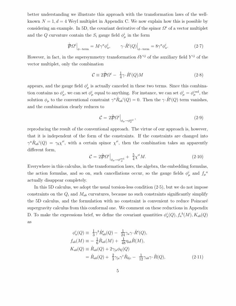
better understanding we illustrate this approach with the transformation laws of the well-

known N = 1, d = 4 Weyl multiplet in Appendix C. We now explain how this is possible by

considering an example. In 5D, the covariant derivative of the spinor Ωi of a vector multiplet

and the Q curvature contain the Si gauge field φiµ in the form

/DΩi∣∣∣φ−term

= Mγaφia, γ ·Ri(Q)

∣∣∣φ−term

= 8γaφia. (2.7)

However, in fact, in the supersymmetry transformation δY ij of the auxiliary field Y ij of the

vector multiplet, only the combination

C ≡ 2 /DΩi − 14γ ·R

i(Q)M (2.8)

appears, and the gauge field φiµ is actually canceled in these two terms. Since this combina-

tion contains no φiµ, we can set φi

µ equal to anything. For instance, we can set φiµ = φi sol

µ , the

solution φµ to the conventional constraint γaRabi(Q) = 0. Then the γ ·Ri(Q) term vanishes,

and the combination clearly reduces to

C = 2 /DΩi∣∣∣φµ→φsol

µ

, (2.9)

reproducing the result of the conventional approach. The virtue of our approach is, however,

that it is independent of the form of the constraints. If the constraints are changed into

γaRabi(Q) = γbχ

′i, with a certain spinor χ′i, then the combination takes an apparently

different form,

C = 2 /DΩi∣∣∣φµ→φ′solµ

+ 54χ

′iM. (2.10)

Everywhere in this calculus, in the transformation laws, the algebra, the embedding formulas,

the action formulas, and so on, such cancellations occur, so the gauge fields φiµ and fµ

a

actually disappear completely.

In this 5D calculus, we adopt the usual torsion-less condition (2.5), but we do not impose

constraints on the Qi and Mab curvatures, because no such constraints significantly simplify

the 5D calculus, and the formulation with no constraint is convenient to reduce Poincare

supergravity calculus from this conformal one. We comment on these reductions in Appendix

D. To make the expressions brief, we define the covariant quantities φia(Q), fa

b(M), Kab(Q)

as

φia(Q) ≡ 1

3γbRi

ab(Q)− 124γaγ ·Ri(Q),

fab(M) ≡ − 16Rab(M) + 1

48ηabR(M),

Kab(Q) ≡ Rab(Q) + 2γ[aφb](Q)

= Rab(Q) + 23γ[aγ

cRb]c − 112γabγ ·R(Q), (2.11)

5

Table I. Weyl multiplet in 5D.

field type remarks SU(2) Weyl-weight

eµa boson funfbein 1 −1

ψiµ fermion SU(2)-Majorana 2 −1

2

bµ boson real 1 0

V ijµ boson V ij

µ = V jiµ = (Vµij)

∗ 3 0

vab boson real, antisymmetric 1 1

χi fermion SU(2)-Majorana 2 32

D boson real 1 2

dependent (unsubstantial) gauge fields

ωµab boson spin connection 1 0

φiµ fermion SU(2)-Majorana 2 1

2

fµa boson real 1 1

where, Rab(M) ≡ Raccb(M), R(M) ≡ Ra

a(M). These quantities are defined in such a way

that they contain the S and K gauge fields in the simple forms

φia(Q)

∣∣∣φ,f

= φia, fab(M)|φ,f = fab, Kab(Q)|φ,f = 0, (2.12)

and Kab(Q) satisfies

γaKab(Q) = 0. (2.13)

Since we impose the torsion-less constraint (2.5) in 5D too, the spin-connection is a dependent

field given by

ωµab = ω0

µab + i(2ψµγ

[aψb] + ψaγµψb)− 2eµ

[abb],

ω0µ

ab ≡ −2eν[a∂[µeν]b] + eρ[aeb]σeµ

c∂ρeσc. (2.14)

Of course, it would also be possible to avoid this torsion-less constraint in a similar way, but

here we follow the conventional procedure.

2.2. The transformation law and the superconformal algebra

The superconformal tensor calculus in 5D can be obtained from the known one in 6D by

carrying out a simple dimensional reduction. However, the Weyl multiplet directly obtained

this way contains 40 + 40 degrees of freedom. Using the procedure explained in detail in

Appendix B, we can separate an 8 + 8 component vector multiplet from it and obtain an

irreducible Weyl multiplet which consists of 32 Bose plus 32 Fermi fields,

eµa, ψi

µ, V ijµ , bµ, vab, χi, D, (2.15)

6

whose properties are summarized in Table I. The full nonlinear Q, S and K transformation

laws of the Weyl multiplet are given as follows. With δ ≡ εiQi + ηiSi + ξaKKa ≡ δQ(ε) +

δS(η) + δK(ξaK),

δeµa = −2iεγaψµ,

δψiµ = Dµε

i + 12v

abγµabεi − γµη

i,

δbµ = −2iεφµ + 2iεφµ(Q)− 2iηψµ − 2ξKµ,

δωµab = 2iεγabφµ − 2iεγ[aRµ

b](Q)− iεγµRab(Q) + 4iεφ[a(Q)eµ

b]

−2iεγabcdψµvcd − 2iηγabψµ − 4ξK[aeµ

b],

δV ijµ = −6iε(iφj)

µ − 2iε(iγaRaµj)(Q)− i

4 ε(iγµγ ·Rj)(Q)

+4iε(iγ ·vψj)µ − i

4 ε(iγµχ

j) + 6iη(iψj)µ ,

δvab = i8 εγabχ− i

8 εγcdγabRcd(Q) + i

2 εRab(Q),

δχi = Dεi − 2γcγabεiDavbc + γ ·R(U)ijε

j

−2γaεiεabcdevbcvde + 4γ ·vηi,

δD = −iε /Dχ− i2 εγ ·vγ ·R(Q)− 8iεRab(Q)vab + iηχ, (2.16)

where the derivative Dµ is covariant only with respect to the homogeneous transformations

Mab, D and U ij (and the G transformation for non-singlet fields under the Yang-Mills group

G). We have also written the transformation law of the spin connection for convenience.The

algebra of the Q and S transformations takes the form

[δQ(ε1), δQ(ε2)] = δP (2iε1γaε2) + δM(2iε1γabcdε2vab) + δU(−4iεi

1γ ·vεj2)

+δS

2iε1γ

aε2φai(Q) + iε1(iγabε2j)Kabj(Q)

+ 332iε1ε2χi + 3

32iε1γaε2γaχi − 1

32iε1(iγabε2j)γabχ

j

+δK

2iε1γbε2fb

a(M) + 112iε

(i1 γ

abcεj)2 Rbcij(U)

+ i6 ε1γ

abcdε2Dbvcd + i2 ε1ε2Dbv

ab

+ 56 iε1γ

aε2v ·v + 83 iε1γ

bε2vbcvca

− 16iε1γ

abcdeε2vbcvde

, (2.17)

[δS(η), δQ(ε)] = δD(−2iεη) + δM(2iεγabη) + δU(−6iε(iηj))

+δK(− 5

6iεγabcηvab + iεγbηvab

), (2.18)

where the translation δP (ξa) is understood to be essentially the general coordinate transfor-

mation δGC(ξλ):

δP (ξa) = δGC(ξλ)− δA(ξλhAλ ). (2.19)

7

Table II. Matter multiplets in 5D.

field type remarks SU(2) Weyl-weight

Vector multiplet

Wµ boson real gauge field 1 0

M boson real 1 1

Ωi fermion SU(2)-Majorana 2 32

Yij boson Y ij = Y ji = (Yij)∗ 3 2

Hypermultiplet

Aαi boson Ai

α = εijAβj ρβα = −(Aα

i )∗ 2 32

ζα fermion ζα ≡ (ζα)†γ0 = ζαTC 1 2

Fαi boson Fα

i ≡ αZAαi , F i

α = −(Fαi )∗ 2 5

2

Linear multiplet

Lij boson Lij = Lji = (Lij)∗ 3 3

ϕi fermion SU(2)-Majorana 2 72

Ea boson real, constrained by (3.15) 1 4

N boson real 1 4

Nonlinear multiplet

Φiα boson SU(2) -valued 2 0

λi fermion SU(2)-Majorana 2 12

V a boson real 1 1

V 5 boson real 1 1

On a covariant quantity Φ with only flat indices, δP (ξa) acts as the full covariant derivative:

δP (ξa)Φ = ξa(∂a − δA(hA

a ))Φ ≡ ξaDaΦ. (2.20)

Note the consistency that the quantities φia(Q) and fa

b(M) on the right-hand side of the

algebra (2.17) cancel out the S and K gauge fields contained in δP (ξa).

§3. Transformation laws of matter multiplets

In 5D there are four kinds of multiplets: a vector multiplet, hypermultiplet, linear multi-

plet and nonlinear multiplet. The components of the matter multiplets and their properties

are listed in Table II. The tensor multiplet in 6D reduces to a vector multiplet in 5D with

constraints, and solving these constraints gives rise to an alternative type of the Weyl mul-

tiplet containing the two-form gauge field Bµν4) in the same way as in 6D. We discuss Bµν

8

in §5.

The supersymmetry transformation laws of the matter multiplets are almost identical

to those obtained in Ref. 9) in the Poincare supergravity case if the ‘central charge vector

multiplet’ components are omitted in the latter.

3.1. Vector multiplet

An important difference between the vector multiplets in 5D and in 6D is the existence

of the scalar component M in 5D, which allows for the introduction of the ‘very special

geometry’ 2) cIJKMIMJMK = 1 in the Poincare supergravity theory. All the component

fields of this multiplet are Lie-algebra valued, e.g., M is a matrix Mαβ = M I(tI)

αβ, where

the tI are (anti-hermitian) generators of the gauge group G. The Q and S transformation

laws of the vector multiplet are given by

δWµ = −2iεγµΩ + 2iεψµM,

δM = 2iεΩ,

δΩi = − 14γ ·F (W )εi − 1

2 /DMεi + Y ijε

j −Mηi,

δY ij = 2iε(i /DΩj) − iε(iγ ·vΩj) − i4 ε

(iχj)M − i4 ε

(iγ ·Rj)(Q)M

−2igε(i[M,Ωj)]− 2iη(iΩj). (3.1)

The gauge group G can be regarded as a subgroup of the superconformal group, and the

above transformation law of the gauge field Wµ provides us with the additional structure

functions, fPQG and fQQ

G. For instance, the commutator of the two Q transformations

becomes

[δQ(ε1), δQ(ε2)] = (R.H.S. of (2.17)) + δG(−2iε1ε2M). (3.2)

For the reader’s convenience, we give here the transformation laws of the covariant deriva-

tive of the scalar DaM and the field strength Fab(W ):

δDaM = 2iεDaΩ − 2iεφa(Q)M + iεγabcΩvbc + 2igεγa[Ω, M ] + 2iηγaΩ + 2ξKaM,

δFab(W ) = 4iεγ[aDb]Ω − 2iεγcd[aγb]Ωvcd + 2iεRab(Q)M − 4iηγabΩ. (3.3)

The transformation laws of a matter field acted on by a covariant derivative and the su-

percovariant curvature (field strength) are derived easily using the simple fact that the

transformation of any covariant quantity also gives a covariant quantity and hence cannot

contain gauge fields explicitly; that is, gauge fields can appear only implicitly in the co-

variant derivative or in the form of supercovariant curvatures, as long as the algebra closes.

Similarly, the Bianchi identities can be computed by discarding the naked gauge fields with

9

no derivative, because both sides of the identity are, of course, covariant. For example, we

have

D[aFbc](W ) = −2iΩγ[aRbc](Q). (3.4)

3.2. Hypermultipet

The hypermultiplet in 5D consists of scalars Aiα, spinors ζα and auxiliary fields F i

α. They

carry the index α (= 1, 2, . . . , 2r) of the representation of a subgroup G′ of the gauge group

G, which is raised (or lowered) with a G′ invariant tensor ραβ (and ραβ with ργαργβ = δαβ )

like Aiα = Aiβρβα. This multiplet gives an infinite dimensional representation of a central

charge gauge group UZ(1), which we regard as a subgroup of the group G. The scalar fields

Aiα satisfy the reality condition

Aiα = εijAβ

j ρβα = −(Aαi )∗, Aiα = (Aiα)∗, (3.5)

and the tensor ραβ can generally be brought into the standard form ρ = ε⊗ 1r by a suitable

field redefinition. Therefor Aiα can be identified with r quaternions. Thus the group G′

acting linearly on the hypermultiplet should be a subgroup of GL(r; H):

δG′(t)Aαi = gtαβAβ

i , δG′(t)Aiα = g(tαβ)∗Ai

β = −gtαβAiβ,

tαβ ≡ ραγt

γδρ

δβ = −(tαβ)∗. (3.6)

Note that the spinors ζα do not satisfy the SU(2)-Majorana condition explicitly, but rather

the USp(2r)-Majorana condition,

ζα ≡ (ζα)†γ0 = ραβ(ζβ)TC = (ζα)TC. (3.7)

The Q and S transformations of the Aiα and ζα are given by

δAiα = 2iεiζα,

δζα = /DAαj ε

j − γ ·vεjAαj −M∗Aα

j εj + 3Aα

j ηj, (3.8)

and with these rules, to realize the superconformal algebra on the hypermultiplet requires

the following two Q and S invariant constraints:

0 = /Dζα + 12γ ·vζ

α − 18χ

iAαi + 3

8γ ·Ri(Q)Aα

i

+M∗ζα − 2Ωi∗Aα

i ,

0 = −DaDaAαi +M∗M∗Aα

i + 4iΩi∗ζα − 2Yij∗Aαj

− i4 ζ

α(χ+ γ ·R(Q)

)+( 3

16R(M) + 18D − 1

4v2)Aα

i , (3.9)

10

where θ∗ = M∗, Ω∗, . . . represents the Yang-Mills transformations with parameters θ, in-

cluding the central charge transformation, that is δG(θ) = δG′(θ) + δZ(θ0). Z denotes the

generator of the UZ(1) transformation and V 0 = (V 0µ ≡ Aµ,M

0 ≡ α,Ω0, Y 0ij) denotes the

UZ(1) vector multiplet. For example, acting on the scalar Aαi , we have

M∗Aαi = gMα

βAβi + αZAα

i . (3.10)

The hypermultiplet in 6D exists only as an on-shell multiplet, since constraints similar to

(3.9) are equations of motion there. Here in 5D, however, it becomes an off-shell multiplet,

as explained in Ref. 9).

First, there appears no constraint on the first UZ(1) transformation of Aαi , so it defines

the auxiliary field

Fαi ≡ αZAα

i , (3.11)

which is necessary for closing the algebra off-shell and balancing the numbers of boson

and fermion degrees of freedom. Next, there are the undefined UZ(1) transformations

Zζα, Z(ZAαi ) (= α−1ZFα

i ) in the constraints (3.9), and therefor we do not interpret the

constraints as the equation of motion but as definitions of these UZ(1) transformations. The

first constraint of (3.9), for example, gives the UZ(1) transformation of the spinor ζα as

Zζα = − α + γaAa

α2 − AaAa

(/D′ζα + 1

2γ ·vζα − 1

8χiAα

i + 38γ ·R

i(Q)Aαi .

+gMαβζ

β − 2gΩiαβAβ

i − 2αΩ

0iFαi

). (3.12)

Note that Daζα contains the UZ(1) covariantization −δZ(Aa)ζα and D′a denotes a covariant

derivative with the −δZ(Aa) term omitted. Also, the second constraint gives the UZ(1) trans-

formation of Fαi , which we do not show explicitly here. Finally, the Q and S transformations

of the auxiliary field Fαi are given by requiring that the UZ(1) transformation commute with

the Q and S transformations on Aαi :

δF iα = δ (δZ(α)Aα

i ) = (δZ(α)δ + δZ(δα))Aαi

= 2iεi(αZζα) + 2iα εΩ

0F iα. (3.13)

3.3. Linear multiplet

The linear multiplet consists of the components listed in Table II and may generally carry

a non-Abelian charge of the gauge group G. This multiplet, apparently, contains 9 Bose and

8 Fermi fields, so that the closure of the algebra on this multiplet requires the constraint

11

(3.15), which can be solved in terms of a three-form gauge field Eµνλ. A four-form gauge

field Hµνρσ can also be introduced for rewriting the scalar component of this multiplet.

The Q and S transformation laws of the linear multiplet are given by

δLij = 2iε(iϕj),

δϕi = − /DLijεj + 12γ

aεiEa + 12ε

iN

+2γ ·vεjLij + gMLijεj − 6Lijηj,

δEa = 2iεγabDbϕ− 2iεγabcϕvbc + 6iεγbϕvab + 2iεiγabcRj

bc(Q)Lij

+2igεγaMϕ− 4igεiγaΩjLij − 8iηγaϕ,

δN = −2iε /Dϕ− 3iεγ ·vϕ+ 12 iε

iχjLij − 32 iε

(iγ ·Rj)(Q)Lij

+4igε(iΩj)Lij − 6iηϕ. (3.14)

The algebra closes if Ea satisfies the following Q and S invariant constraint:

DaEa + iϕγ ·R(Q) + gMN + 4igΩϕ+ 2gY ijLij = 0. (3.15)

This constraint can be separated into two parts, a total derivative part and the part propor-

tional to the Yang-Mills coupling g:

e−1∂λ(eVλ) + 2ge−1HV L = 0, (3.16)

where, Va and HV L are given by

Va = Ea − 2iψbγbaϕ+ 2iψbγ

abcLψc,

e−1HV L = Y ijLij + 2iΩϕ+ 2iψai γaΩjL

ij − 12WaVa

+ 12M

(N − 2iψbγ

bϕ− 2iψ(ia γ

abψj)b Lij

). (3.17)

When the linear multiplet is inert under the G transformation, that is g = 0, this constraint

can be solved in terms of a three-form gauge field Eµνλ as Vλ = e−1ελµνρσ∂µEνρσ/6, which

possesses the additional gauge symmetry δE(Λ)Eµνλ = 3∂[µΛνλ]. Hence the linear multiplet

becomes an unconstrained multiplet (Eµνλ, Lij, ϕi, N).

It shoud be noted that in 6D, the linear multiplet requires a similar constraint on the

6D vector Ea, and this constraint can be solved in terms of the four-form gauge field Eµνρσ

in a similar manner. This 6D four-form field yields a three-form field Eµνλ and a four-form

field Hµνρσ through the simple reduction, while the 6D vector Ea reduces to the 5D vector

Ea and the scalar N . Thus we expect that the scalar field N can be rewritten in terms of

a four-form field Hµνρσ in this 5D linear multiplet. (Note the number of degrees of freedom

of the Hµνρσ is 1 in 5D.) The quantity HV L contains N , and any transformation of this

12

quantity becomes a total derivative, because the constraint (3.16) is invariant under the full

transformations. Thus it can be rewritten with Hµνρσ in the form

2HV L = − 14!ε

λµνρσ∂λ(Hµνρσ − 4WµEνρσ), (3.18)

where the extra term W[µEνρσ] on the right hand-side is inserted for later convenience. With

this rewriting, the constraint (3.16) can be solved even for the case that the linear multiplet

carries a charge of the gauge group G. Indeed, since the r.h.s. of (3.18) is a total derivative,

we have

e−1∂λ

eVλ − g

4!ελµνρσ(Hµνρσ − 4WµEνρσ)

= 0

→ Vλ = 14!e

−1ελµνρσ(4∂[µEνρσ] − 4gWµEνρσ + gHµνρσ

). (3.19)

The transformation laws of Eµνλ and Hµνρσ must be determined up to the additional gauge

symmetry δH(Λ)Hµνρσ = 4(∂[µ − gW[µ)Λνρσ], δH(Λ)Eµνλ = −gΛµνλ, so that the all transfor-

mation laws of both sides of (3.19) are the same for consistency. Also the transformation laws

of the tensor gauge fields defined in this way are consistent with the replacement equation

(3.18), because this equation is satisfied automatically due to the invariant equations (3.16)

and (3.19). Now, let us rewrite the replacement equation of N , (3.18), and the solution of

Ea, (3.19), into the following two invariant equations:

Ea = 14!ε

abcdeFbcde(E),

MN + 2YijLij + 4iΩϕ = − 1

5!εabcdeFabcde(H). (3.20)

The quantities Fabcd(E) and Fabcde(H) are the field strengths given by

Fµνρσ(E) = 4D[µEνρσ] + gHµνρσ + 8iψ[µγνρσ]ϕ+ 24iψi[µγνρψ

jσ]Lij ,

Fλµνρσ(H) = 5D[λHµνρσ] − 10F[λµ(W )Eνρσ]

−10iψ[λγµνρσ]Mϕ + 20iψi[λγµνρσ]λ

jLij − 40iψi[λγµνρψ

jσ]MLij ,

(3.21)

where the derivative Dµ is covariant with respect to the G transformation:Dµ ≡ ∂µ − gWµ.

The transformation laws of Eµνλ and Hµνρσ can be understand from the fact that the left-

hand sides of the equations in (3.20) are covariant under the full transformation, and so the

field strengths on the r.h.s. must also be fully covariant. With δ ≡ δQ(ε) + δS(η) + δG(Λ) +

δE(Λµν) + δH(Λµνλ), we have

δEµνλ = 3D[µΛνλ] + gΛEµνλ − gΛµνλ − 2iεγµνλϕ− 12iεiγ[µνψjλ]Lij ,

δHµνρσ = 4D[µΛνρσ] + gΛHµνρσ + 6F[µν(W )Λρσ]

+2iεγµνρσMϕ− 4iεiγµνρσΩjLij

+16iεiγ[µνρψjσ]MLij + 4(δQ(ε)W[µ)Eνρσ]. (3.22)

13

These transformation laws are truly consistent with (3.20), and thus with (3.19). With these

laws, the following modified algebra closes on the tensor gauge fields Eµνλ and Hµνρσ:

[δQ(ε1), δQ(ε2)] = (R.H.S. of (3.2)) + δE(4iεi1γµνε

j2Lij)

+δH(4iεi

1γµνλεj2MLij − 2iε1ε2MEµνλ

),

[δQ(ε), δE(Λµν)] = δH(3δQ(ε)W[µΛνλ]

),

[δG(Λ), δE(Λµν)] = δE(−gΛΛµν), [δG(Λ), δH(Λµνλ)] = δH(−gΛΛµνλ).

(3.23)

This fact also justifies the replacement (3.18) algebraically. Nevertheless, in order to actually

claim that (Eµνλ, Hµνρσ, Lij , ϕi) gives a new version of the linear multiplet, we must show

that the component N can be expressed in terms of Hµνρσ by solving (3.18). The point is

that the left hand side of (3.18) HV L contains N in the form MN , but the Lie-algebra valued

scalar M is, of course, not always invertible. In some particular cases, the matrix M can

be invertible. For example, the determinant of the SU(2)-valued matrix Ma(σa/2) does not

vanish in the domain∑3

a=1MaMa 6= 0. Therefor, the linear multiplet can take the doublet

representation of SU(2) as a subgroup of G in this domain.

3.4. Nonlinear multiplet

A nonlinear multiplet is a multiplet whose component fields are transformed nonlinearly.

The first component, Φiα, carries an additional gauge-group SU(2) index α (= 1, 2), as well

as the superconformal SU(2) index i. The index α is also raised (and lowered) by using the

invariant tensor εαβ (and εαβ with εγαεγβ = δαβ ) as Φi

α = Φiβεβα. The field Φiα takes values in

SU(2) and hence satisfies

ΦiαΦ

αj = δi

j , Φαi Φ

iβ = δα

β . (3.24)

The Q, S and K transformation laws of this multiplet are given by

δΦαi = 2iε(iλj)Φ

jα,

δλi = −Φiα /DΦα

j εj +MαβΦ

αiΦβjεj + γ ·vεi

+ 12γ

aVaεi + 1

2V5εi − 2iεjλiλj − 3ηi,

δVa = 2iεγabDbλ− iεγaγ ·V λ+ iεγaλV5

+2iεγbλvab + 14iεγaχ+ 2iεγbRab(Q)− iεγaγ ·R(Q)

+2iεiγaΦαi /DΦαj λ

j − 4igεiγaΩjαβΦ

αi Φ

βj − 2igεiγaλ

jMαβΦαi Φ

βj

−2iηγaλ− 6ξKa,

14

δV 5 = −2iε /Dλ+ iεγ ·V λ− iελV 5 − iεγ ·vλ− 14iεχ + 3

4iεγ ·R(Q)

−2iεiΦαi /DΦαj λ

j + 4igεΩjαβΦ

αi Φ

βj + 2igεiλjMαβΦ

αi Φ

βj .

(3.25)

As in the linear multiplet case, the nonlinear multiplet also needs the following Q, S and K

invariant constraint for the closure of the algebra:

DaVa − 12VaV

a + 12(V 5)2 + DaΦi

αDaΦαi + 2iλ /Dλ

+2iλiΦαi /DΦαj λ

j + iλγ ·vλ+ 3

8R(M) + 14D − 1

2v2 + i

2 λχ−i2 λγ ·R(Q)

+2gY ijαβΦ

αi Φ

βj − 8igλiΩj

αβΦαi Φ

βj − 2igλiλjMαβΦ

αi Φ

βj

+g2MαβM

βα = 0. (3.26)

This constraint can be solved for the scalar of the Weyl multiplet D, and this solution

presents us with a new (40+40) Weyl multiplet, which possesses the unconstrained nonlinear

multiplet instead of D.

§4. Embedding and invariant action formulas

4.1. Embedding formulas

We now give some embedding formulas that give a known type of multiplet using a (set

of) multiplet(s).

To determine embedding formulas that give the linear multiplet L by means of other

multiplets is not difficult for the following reason. When the transformation of the lowest

component Lij of a multiplet takes the form 2iε(iϕj), the superconformal algebra consisting

of (2.17) and (2.18) demands that all the other higher components must uniquely transform

in the form given in Eq. (3.14) and that the constraint (3.15) should hold. Therefore, in

order to identify all the components of the linear multiplet, we have only to examine the

transformation law up to the second component ϕi, as long as the algebra closes on the

embedded multiplets.

The vector multiplets can be embedded into the linear multiplet with arbitrary quadratic

homogeneous polynomials f(M) of the first components M I of the vector multiplets. The

index I labels the generators tI of the gauge group G, which is generally non-simple. These

embedding formulas L(V ) are

Lij(V ) = Y IijfI − iΩI

i ΩJj fIJ ,

15

ϕi(V ) = − 14

(χi + γ ·Ri(Q)

)f

+(

/DΩIi − 1

2γ ·vΩIi − g[M,Ω]I

)fI

+(− 1

4γ ·FI(W )ΩJ + 1

2 /DM IΩJ − Y IΩJ)fIJ ,

Ea(V ) = Db(4vabf + F I

ab(W )fI + iΩIγabΩJfIJ

)+(−iΩIγabcR

bc(Q)− 2ig[Ω, γaΩ]I + g[M, DaM ]I)fI

+(−2igΩIγa[M,Ω]J + 1

8εabcdeFbcI(W )F deJ(W )

)fIJ ,

N(V ) = −DaDaf +(− 1

2D + 14R(M)− 3v ·v

)f

+(−2Fab(W )vab + iχΩI + 2ig[Ω, Ω]I

)fI

+

− 1

4 FIab(W )F abJ(W ) + 1

2DaM IDaM

J

+2iΩI /DΩJ − iΩIγ ·vΩJ + Y IijY

Jij

fIJ , (4.1)

where the commutator [X, Y ]I represents [X, Y ]ItI ≡ XIY J [tI , tJ ], and

f ≡ f(M), fI ≡∂f

∂M I, fIJ ≡

∂2f

∂M I∂MJ. (4.2)

Here, it is easy to see that we cannot generalize the function f(M) further. For example,

the lowest component Lij is S invariant. Thus the right-hand side of the first equation of

this formula has to be S invariant, and this fact requires M IfI = 2f . Therefore f(M) must

be a homogeneous quadratic function of the scalar field M : f(M) = fIJMIMJ/2.

The product of the two hypermultiplets H = (Aiα, ζα, F i

α) and H ′ = (A′iα, ζ

′α, F ′i

α) can

also compose a linear multiplet L(H ,H ′) as follows:

Lijαβ(H ,H ′) = A(i

αA′j)β ,

ϕiαβ(H ,H ′) = ζαA′i

β + ζ ′βAiα,

Eaαβ(H ,H ′) = Ai

αDaA′βi +A′i

βDaAαi − 2iζαγaζ ′β,

Nαβ(H ,H ′) = −AiαM∗A′

βi −A′iβM∗Aαi − 2iζαζ

′β. (4.3)

Here, this linear multiplet transforms non-trivially under the UZ(1) transformation, in addi-

tion to the transformations that are self-evident from the index structure; e.g., δZ(α)Lijαβ =

F (iαA′j)

β + A(iαF

j)β . For this multiplet, therefore, the ‘group action terms’, like gMLij ap-

pearing in the Q transformation law (3.14), and the action formula, which we discuss in

the next subsection, should be understood to contain not only the usual gauge group action

but also the U(1) action: gM → M∗ = δG′(M) + δZ(α). Also note that ZnH with the

arbitrary number n can be substituted for H and H ′ in the above formulas, because ZH

also transforms as a hypermultiplet.

16

Conversely, we can also embed the linear multiplet into the vector multiplet. The fol-

lowing combination of the components of the linear multiplet is S invariant and carries

Weyl-weight 1:

M(L) = NL−1 + iϕiϕjLijL−3, (4.4)

with L =√LijLij . This embedding formula is a non-polynomial function of the field, and for

this reason, the embedding formulas for the higher components becomes quite complicated.

Though we have not confirmed that the embedding (4.4) is consistent with the transforma-

tion laws of the higher components, this formula agrees with the formula in the Poincare

supergravity in 5D presented by Zucker 12) up to the components of the ‘central charge vector

multiplet’. Thus it must be a correct form.

4.2. Invariant action formula

The quantity HV L appearing in (3.17) transforms into a total derivative under all of the

gauge transformations and has Weyl-weight 5. It therefor represents a possibility as the

invariant action formula. However (3.16) implies that HV L itself is a total derivative and

so cannot give an action formula. Fortunately, the invariant action formula can be found in

the following way with a simple modification of the expression of HV L. Let us consider the

action formula

e−1L(V ·L) ≡ Y ij · Lij + 2iΩ · ϕ+ 2iψai γaΩj · Lij

− 12Wa ·

(Ea − 2iψbγ

baϕ+ 2iψ(ib γ

abcψj)c Lij

)+ 1

2M ·(N − 2iψbγ

bϕ− 2iψ(ia γ

abψj)b Lij

), (4.5)

where the dot (e.g. that in V ·L) indicates a certain suitable operation. If this dot represents

theG transformation ∗ defined by gV ∗L ≡ δG(V )L, then this formula reduces to the original

HV L [= L(V ∗L)]. The Q and G transformation law of L(L ·V ) may be different from that

of HV L only in the terms proportional to g. For the Q transformation, for instance, we have

δQ(ε)L(V ·L) = (total derivative)

+2giεiγa[Wa, Ωj ; Lij ] + 2giεi[M, Ωj ; Lij ]

+giεγa[M, Wa; ϕ] +gi2 εγ

ab[Wa, Wb; ϕ]

+giεγabc[Wa, Wb; L]ψc + 2giεγab[M, Wa; L]ψb, (4.6)

where [A, B; C] denotes the following Jacobi-like operation:

[A, B; C] ≡ A · (B ∗ C)− B · (A ∗ C)− (A ∗B) · C. (4.7)

17

The G transformation of (4.5) also takes a similar form. Hence if we find a dot operation

(·) for which (4.7) identically vanishes, then the action formula (4.5) will be invariant up to

the total derivative under the Q and G transformation, in addition to the S transformation.

(Of course if we choose · as ∗, the operation (4.7) vanishes, as the Jacobi identity.)

For instance, we can see from (4.6) that the action formula (4.5) gives an invariant by

taking the dot operation to be a simple product, if the vector multiplet is Abelian and the

linear multiplet carries no gauge group charge or is charged only under the Abelian group of

this vector multiplet, like the central charge transformation δZ . When the linear multiplet

carries no charges at all, the constrained vector field Ea can be replaced by the three-form

gauge field Eµνλ. Using this, the third line of the above action (4.5) can be rewritten, up to

total derivative, as

− 12Wa

(Ea − 2iψbγ

baϕ+ 2iψ(ib γ

abcψj)c Lij

)→ − 1

4!εµνλρσFµν(W )Eλρσ. (4.8)

Similarly replacing ∗ by · in Eq. (3.18), we can obtain another invariant action formula

written in terms of the four-form gauge field Hµνρσ. This gives an off-shell formulation of the

SUSY-singlet ‘coupling field’ introduced in Ref. 20), as will be discussed in a forthcoming

paper. 21)

The action formula (4.5) can be used to write the action for a general matter-Yang-

Mills system coupled to supergravity. If we use the above embedding formula, (4.1), of

the vector multiplets into a linear multiplet and apply the action formula (4.5) and (4.8),

LV = L(V ALA(V )

), then we obtain a general Yang-Mills-supergravity action. Although

the action formula can be applied only to the Abelian vector multiplets V A, interestingly

V A can be extended to include the non-Abelian vector multiplets V I in this Yang-Mills

action; that is, the quadratic function fA(M) multiplied by MA can be extended to a cubic

function N (M) as − 16fA,IJM

AM IMJ → N = cIJKMIMJMK . Also, the action for a

general hypermultiplet matter system can be obtained similarly. The kinetic term for the

hypermultiplet is given by LHkinetic = L(A dαβLαβ(H , ZH)

), with the central charge vector

multiplet A = V 0 and an antisymmetric G invariant tensor dαβ. The mass term for the

hypermultiplet are given by LHmass = L(A ηαβLαβ(H ,H)

), with a symmetric G invariant

tensor ηαβ. Finally, the action for the unconstrained linear multiplet is given by LL =

L (V (L) L), which may contain a kinetic term for the four-form field Hµνρσ in addition to

that for Eµνλ. These actions in the superconformal tensor calculus must be identified with

those in the Poincare supergravity tensor calculus.

In the case that the linear multiplet carries a non-Abelian charge, the invariant action

cannot be obtained in a simple way: If we assume that the linear multiplet is Lie-algebra

valued and interpret the dot operation as a trace, then the Jacobi-like operation (4.7) does

18

not vanish. However, it is not impossible to obtain this action. For example, one can consider

Abelian vector multiplets V α carrying a non-Abelian charge. That is,

[GI , Gα] = fIαβGβ = −ρ(GI)β

αGβ, [Gα, Gβ] = 0, (4.9)

where GI and Gα are generators of non-Abelian and Abelian generators, respectively. The

linear multiplet is also assumed to be an ajoint representation of this group, (LI ,Lα). Then

the Jacobi-like operation (4.7) vanishes if we take the dot operation to be given by

A · B = AαBα = ραβA

αBβ = −B ·A, ραβ = −ρβα, (4.10)

and L(V αLβραβ) gives an invariant action, while the linear multiplet carries a non-Abelian

charge.

§5. The two-form gauge field and Nishino-Rajpoot formulation

To this point in the text, the three-form gauge field Eµνλ and the four-form gauge fields

Hµνρσ have appeared, in addition to the one-form gauge fieldsWµ. A two-form gauge field Bµν

can also be introduced in the process by solving the constraint L0(V ) = 0, which we impose

on a set of Vector multiplets V I using an embedding quadratic formulation f0(M). The

solution leads to another type of the Weyl multiplet that contains Bµν . The formulation with

this new multiplet gives the alternative supergravity presented by Nishino and Rajpoot 4)

after suitable S and K gauge fixing. (Thus we will call this the ‘N-R formulation’.)

Here, we choose the quadratic function f0(M) to beG inert: [A,B]ICJf0,IJ+BI [A,C]Jf0,IJ =

0. Then, we solve the equation L0(V ) = 0. The equation Lij(V ) = 0 sets one of the aux-

iliary fields Y Iij of the vector multiplets V I equal to zero. The equation ϕi(V ) = 0 makes

the auxiliary spinor field χi of the Weyl multiplet a dependent field, and similarly the equa-

tion N(V ) = 0 is solved with respect to the auxiliary scalar field D of the Weyl multiplet.

Then, the equation Ea(V ) = 0 becomes a total derivative in this gauge-invariant case, as

mentioned above:

Eµ(V ) = e−1∂ν

( 16ε

µνλρσEλρσ(V ))

= e−1∂ν

e(4vµνf + F µνI(W )fI + iΩIγµνΩJfIJ

+iψργµνρσψσf − 2iψλγ

µνλΩIfI

)+ 1

2εµνλρσ

(W I

λ∂ρWJσ −

13gW

Iλ [Wρ, Wσ]J

)fIJ

= 0. (5.1)

Thus this equation is also solved by making the auxiliary tensor field vab dependent. However,

the last equation here does not fix all components of vab, because Ea and vab have 4 and 10

19

degrees of freedom, respectively. Of course the equation can be solved by means of adding

the two-form field Bµν , which has 6 degrees of freedom: 0 = Eµνλ(V ) + 3∂[µBνλ]. This can

also be rewritten as

0 = Fµνλ(B)− 12eεµνλρσ(4vρσf + F ρσI(W )fI) + iΩIγµνλΩ

JfIJ , (5.2)

where Fµνλ(B) is the covariant field strength of Bµν , which is given by

Fµνλ(B) = 3∂[µBνλ] − 6iψ[µγνλ]ΩIfI + 6iψ[µγνψλ]f

−3∂[µWIνW

Jλ]fIJ +W I

[µ[Wν , Wλ]]JfIJ . (5.3)

A Q and G transformation law of Bµν can be easily found from the Q and G covariance

of (5.3) in the same way as that of Hµνρσ and Eµνλ in the linear multiplet case. The gauge

field Bµν is S invariant and transforms under δ = δQ(ε) + δB(ΛBµ ) + δG(Λ) as

δBµν = 2iεγµνΩIfI − 4iεγ[µψν]f + (δQ(ε)W I

[µ)WJν]fIJ

+2∂[µΛBν] + ∂[µW

Iν]Λ

JfIJ . (5.4)

The algebra on Bµν , of course, closes, although the algebra is modified as follows:

[δQ(ε1), δQ(ε2)] = (R.H.S. of (3.2)) + δB(−2iε1γµε2f − iε1ε2W

IµfI

),

[δQ(ε), δG(Λ)] = δB(δQ(ε)W I

µΛJfIJ

),

[δG(Λ1), δG(Λ2)] = δB(− 1

2WIµ [Λ1, Λ2]

JfIJ

)+ δG (−[Λ1, Λ2]) . (5.5)

Now the constraint equations L0(V ) = 0 has replaced the ‘matter’ sub-multiplet (vab, χi, D)

of the Weyl multiplet by the tensor field Bµν and a linear combination of the vector multi-

plets with one component of the auxiliary field Y Iij eliminated. We thus have obtained the

N-R formulation with an alternative Weyl multiplet. If we take only a single vector multi-

plet, say the central vector multiplet, V 0 = (α, Aµ, Ω0i, Y 0ij), and set f0(M) = α2, then

the conventional Weyl multiplet (eµa, ψi

µ, bµ, Vijµ , vab, χ

i, D) is replaced by a new 32 + 32

multiplet consisting of (eµa, ψi

µ, bµ, Vijµ , Bµν , Aµ, α, Ω

0i).

There are two known different types of formulations of the on-shell supergravity in 5D, the

conventional one with no Bµν and the above N-R formulation. These different formulations

give different physics of course. From the point of view of off-shell formulation, this difference

is only a difference in the cubic function N (M) that characterizes super Yang-Mills systems

in 5D. If there is an Abelian vector multiplet VNR that appears only in the form of a Lagrange

multiplier, that is, if N takes the form

N = cIJKMIMJMK +MNRfIJM

IMJ , (5.6)

20

and if matter multiplets carry no charge of this vector multiplet, then the equations of motion

take the form L0(V ) = 0 by the variation of VNR. Therefore, after integrating out VNR,

the N-R formulation appears. Conversely, if there is no such Abelian vector multiplet, the

formulation gives the conventional one.

§6. Summary and comments

In this paper, we have presented a superconformal tensor calculus in five dimensions.

This work extends a previous work, 9) which presents Poincare supergravity tensor calculus

that is almost completely derived using dimensional reduction and decomposition from the

known superconformal tensor calculus in six dimensions. The significant difference between

the superconformal tensor calculus presented in this paper and Poincare one is that the

minimal Weyl multiplet in the superconformal case has 32 Bose plus 32 Fermi degrees of

freedom, while that in the Poincare case has (40+40) degrees of freedom.

In a previous paper, 10) we constructed off-shell d = 5 supergravity coupled to a matter-

Yang-Mills system by using the Poincare supergravity tensor calculus. 9) There, intricate and

tedious computations were necessary (owing to a lack of S symmetry) to rewrite the Einstein

and Rarita-Schwinger terms into canonical form. However, now we can write down the same

action with little work, thanks to the full superconformal symmetry. Actually, we can show

readily that this superconformal calculus is equivalent to two Poincare calculuses with two

different S gauge choices, and thus the two Poincare calculuses are equivalent (see Appendix

D). Also, it is easy to show the equivalence to other Poincare supergravities. 2) - 4)

There appeared several by-products in the text. In this calculus, we have not imposed

constraints on the Q and M curvatures. Though this is a purely technical point and unim-

portant from the viewpoint of physics, it could be interesting to pursue, as it is different

from usual situation in superconformal gravities. This formulation with no constraints makes

clear that these constraints are completely unsubstantial. It is thus seen that superconformal

gravity with various forms of constraints can describe the same physics.

Moreover, the four-form gauge fieldHµνρσ and the two-form gauge field Bµν have appeared

in this off-shell formulation in addition to the three-form gauge field Eµνλ.

In recent studies of the brane world scenario, the four-form gauge field Hµνρσ plays an

important role in connection with the Q singlet scalar ‘coupling field’ G. Now we can

construct an off-shell formulation of Hµνρσ and G, though only an on-shell formulation is

known to this time. This extension may allow for the extraction of general properties from

the brane world scenario without going into the details of the models. This will be discussed

in a forthcoming paper. 21) Also L (V (L)L) may contain a kinetic term for Hµνρσ and lead

21

to interesting physics in the brane world scenario.

Introducing the two-form gauge field Bµν implies a new non-minimal Weyl multiplet,

which should be equivalent to that presented by Nishino and Rajpoot. 4) From the viewpoint

of the off-shell formalism, this system is unified with the general matter Yang-Mills system.2), 3)

The tensor multiplet as a matter multiplet, containing a two-form gauge field Bµν , is

known in on-shell formulation. But we have not yet understood it in the present tensor cal-

culus. Excluding this problem, however, this superconformal tensor calculus shoud produce

all types of supergravity in 5D. Superconformal tensor calculus will provide powerful tools

for the brane world scenario from a more unified viewpoint.

Acknowledgements

The authors would like to thank Professor Taichiro Kugo for helpful discussions and

careful reading of the manuscript.

Appendix A

Conventions and Useful Identities

We employ the notation of Ref. 9). The gamma matrices γa satisfy γa, γb = 2ηab and

(γa)† = ηabγ

b, where ηab = diag(+,−,−,−,−). γa...b represents an antisymmetriced product

of gamma matrices:

γa...b = γ[a . . . γb], (A.1)

where the square brackets denote complete antisymmetrization with weight 1. Similarly (. . .)

denote complete symmetrization with weight 1. We chose the Dirac matrices to satisfy

γa1...a5 = εa1...a5 (A.2)

where εa1...a5 is a totally antisymmetric tensor with ε01234 = 1. With this choice, the duality

relation reads

γa1...an =(−1)n(n−1)/2

(5− n)!εa1...anb1...b5−nγb1...b5−n . (A.3)

The SU(2) index i (i=1,2) is raised and lowered with εij , where ε12 = ε12 = 1, in the

northwest-southeast (NW-SE) convention:

Ai = εijAj , Ai = Ajεji. (A.4)

22

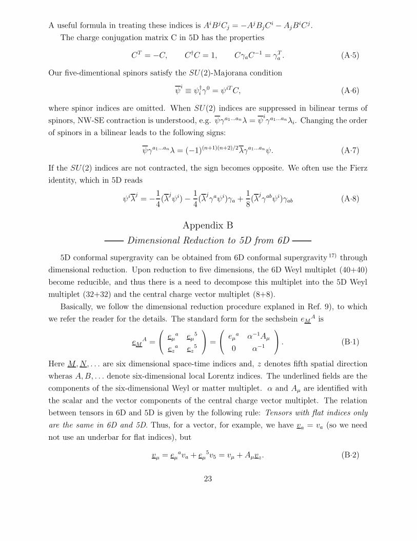
A useful formula in treating these indices is AiBjCj = −AjBjCi − AjB

iCj .

The charge conjugation matrix C in 5D has the properties

CT = −C, C†C = 1, CγaC−1 = γT

a . (A.5)

Our five-dimentional spinors satisfy the SU(2)-Majorana condition

ψi ≡ ψ†iγ

0 = ψiTC, (A.6)

where spinor indices are omitted. When SU(2) indices are suppressed in bilinear terms of

spinors, NW-SE contraction is understood, e.g. ψγa1...anλ = ψiγa1...anλi. Changing the order

of spinors in a bilinear leads to the following signs:

ψγa1...anλ = (−1)(n+1)(n+2)/2λγa1...anψ. (A.7)

If the SU(2) indices are not contracted, the sign becomes opposite. We often use the Fierz

identity, which in 5D reads

ψiλj

= −1

4(λ

jψi)− 1

4(λ

jγaψi)γa +

1

8(λ

jγabψi)γab (A.8)

Appendix B

Dimensional Reduction to 5D from 6D

5D conformal supergravity can be obtained from 6D conformal supergravity 17) through

dimensional reduction. Upon reduction to five dimensions, the 6D Weyl multiplet (40+40)

become reducible, and thus there is a need to decompose this multiplet into the 5D Weyl

multiplet (32+32) and the central charge vector multiplet (8+8).

Basically, we follow the dimensional reduction procedure explaned in Ref. 9), to which

we refer the reader for the details. The standard form for the sechsbein eMA is

eMA =

eµ

a eµ5

eza ez

5

=

eµ

a α−1Aµ

0 α−1

. (B.1)

Here M,N, . . . are six dimensional space-time indices and, z denotes fifth spatial direction

wheras A,B, . . . denote six-dimensional local Lorentz indices. The underlined fields are the

components of the six-dimensional Weyl or matter multiplet. α and Aµ are identified with

the scalar and the vector components of the central charge vector multiplet. The relation

between tensors in 6D and 5D is given by the following rule: Tensors with flat indices only

are the same in 6D and 5D. Thus, for a vector, for example, we have va = va (so we need

not use an underbar for flat indices), but

vµ = eµava + eµ

5v5 = vµ + Aµvz. (B.2)

23

We decompose the six-dimensional gamma matrices ΓM and the charge conjugation matrix

C as

Γ a = γa ⊗ σ1, Γ 5 = 1⊗ iσ2,

C = C ⊗ iσ2. (B.3)

The six-dimensional chirality operator Γ7 is written Γ7 = 1⊗σ3. The six dimensional SU(2)-

Majorana-Weyl spinor ψi±, which satifies the SU(2)-Majorana condition ψ

i

± ≡ ψ†i±Γ0 = ψiT

± C

and the Weyl condition Γ7ψi± = ±ψi

±, is decomposed as

ψi+ = ψi ⊗

1

0

, ψi

− = iψi ⊗ 0

1

, (B.4)

where ψi is a five-dimensional SU(2)-Majorana spinor.

The generators of 6D superconformal algebra, which is Osp(8∗|2), are labeled

PA, MAB, KA, D, Uij , Qiα, S

iα. (B.5)

Of these, the generators Ma5 and K5 are redundant in 5D and are used to fix redundant

gauge fields, as described below. The independent gauge fields of the N = 2, d = 6 Weyl

multiplet, which realize this algebra are

eMA, ψi

M+, bM , V

ijM , T

−ABC , χ

i−, D. (B.6)

The first four are the gauge fields corresponding to the generators PA,Qiα,D and U ij . The

last three are the additive matter fields. The other gauge fields, ωMAB, φi

Mand f

MA, which

correspond to the generators MAB, Siα and KA can be expressed in terms of the above

independent gauge fields by imposing the curvatures constraints

RMNA(P ) = 0,

RMNAB(M)eN

B + T−MBCT−ABC +

1

12eM

AD = 0,

ΓNRi

MN(Q) = − 1

12ΓMχ

i, (B.7)

where RMNA(P ), RMN

AB(M) and Ri

MN(Q) are the P , M and Q curvatures, respectively.

(For more details, see Ref. 17), but note that we use the notation of Ref. 9).)

First, we decompose the six-dimensional Weyl multiplet into three classes,

( eµa, ψi

µ, bµ, V

ijµ , T

−ab5, χ

i, D ),

( eµ5, ez

5, ψiz, V ij

z ),

( eza, bz ). (B.8)

24

Roughly speaking, the first class gives the five-dimensional Weyl multiplet and the second the

central charge vector multiplet. The last class consists of redundant gauge fields. Redundant

gauge fields can be set equal to zero as a gauge-fixing choice for the redundant Ma5 and

K5 symmetries. However, the condition eza = bz = 0 is not invariant under Q and S

transformations. Thus, we have to add a suitable gauge transformation to the original Q

and S transformations. Explicitly, the original Q transformation of eza is

δ6DQ (ε)ez

a = −2iεγaψz. (B.9)

Adding a Ma5 transformation with parameter θa5M = −2iαεγaψ

zto the original Q transfor-

mation, we obtain a Q transformation, under which the constraint eza = 0 remains invariant.

Similarly, in order to keep bz = 0 invariant under Q and S transformations, we should add a

K5 transformation with parameter θ5K(ε) = iεχ/24 + iεφ

5to the original Q transformation

and a K5 transformation with parameter ζ5K(η) = iηψ

zto the original S transformation,

δ6DS (η).

In the original gauge transformation law for fields of the first class, the central charge

vector multiplet components do not decouple. For example, the Q transformation of ψiµ

is

δ6DQ (ε)ψi

µ= Dµε

i − 1

4T ρσ−

5 γµρσεi +

1

2α∂[µAν]γ

νεi − 2i(εγµψz)ψi

z+ . . . . (B.10)

This transformation includes α = ez5, Aµ = αeµ

5 and ψz, which are the fields of the cen-

tral charge vector multiplet. To get rid of these fields from the transformation law of the

five-dimensional Weyl multiplet, we need to redefine the gauge fields and the Q and S trans-

formations. The proper identification of the central charge vector multiplet components

turns out to be

α = ez5, Aµ = αeµ

5, Ωi0 = −α2ψi

z, Y ij

0 = α2V ijz −

3i

αΩ

i0Ω

j0. (B.11)

The field α, whose Weyl weight is 1, is used to adjust the Weyl weight of the redefined field.

For example, Aµ should carry Weyl weight 0 as any gauge field, but the Weyl weight of eµ5

is −1, so we identify αeµ5 with the gauge field Aµ. The correction term 3iΩ

i0Ω

j0/α in the

redefinition of Y ij0 is needed to remove the central charge vector multiplet from the algebra.

Similarly, the irreducible (32+32) Weyl multiplet in 5D is identified as

eµa = eµ

a, ψiµ = ψi

µ, bµ = bµ,

V ijµ = V ij

µ +2i

αψ

(i

µΩj)0 − i

α2Ω

i0γµΩ

j0,

vab = −T−ab5 −1

4αFab(A) +

i

2α2Ω0γabΩ0,

25

χi =16

15χi +

8

5α

(D/Ωi

0 +1

2α(D/ α)Ωi

0 +3

2γ · vΩi

0

)

−1

5

(γ · Ri(Q)− 6

α2γ · F (A)Ωi

0

)− 8

α2tijΩ0j −

2i

α3γabΩ

i0Ω0γ

abΩ0,

D =8

15D − 1

10Rab

ab(M) + 2vabvab

+1

α

(iΩ0χ +

4i

5Ω0γ · R(Q)

)− 4

5αDaDaα− 2

5α2DaαDaα

+2

5α2Fab(A)F ab(A)− 4

α2tijt

ij +O(Ω20), (B.12)

where O(Ω20) represents terms of higher order in Ω0.

The relation between the Q and S transformations in 5D and in 6D is finally given by

δQ(ε) = δ6DQ (ε) + δM(θM (ε)) + δU (θU(ε)) + δS(θS(ε)) + δK(θK(ε)),

δS(η) = δ6DS (η) + δK(ζK(η)), (B.13)

where

θa5M (ε) =

2i

αεγaΩ0, θij

U (ε) = −2i

αε(iΩ

j)0 ,

θiS(ε) =

1

4γ ·(−v +

1

4αF (A)

)εi − i

2α2(Ω

i0Ω

j0)εj +

i

2α2(Ω

i0γaΩ

j0)γ

aεj ,

θKµ(ε) = − i

24εγµχ− iε

(φ

µ− θSµ(

Ω0

α)− φµ

)− iεφa(Q),

θ5K(ε) =

i

24εχ+ iε

(φ

5− θS(

Ω0

α)), ζ5

K(η) = − i

αηΩ0. (B.14)

Here, the dependent gauge fields φiµ

and φi5

are those determined by the curvature constraint

(B.7).

The 6D vector multiplet consists of a real vector field WM , an SU(2)-Majorana spinor

Ωi, and a triplet of the auxiliary scalar field Y ij , whereas the 5D vector multiplet consists of

a real vector Mµ, a scalar M , an SU(2) Majorana spinor Ωi, and a triplet of the auxiliary

scalar Y ij . The proper identification of the vector multiplet components is

M = −W 5, Wµ = W µ, Ωi = Ωi +M

αΩi

0,

Y ij = Y ij +M

αY ij

0 − 2i

αΩ

(i0

(Ωj) − M

αΩ

j)0

). (B.15)

The 6D linear multiplet consists of a triplet Lij, an SU(2)-Majorana spinor ϕi, and a

constrained vector field EA. The components of the 5D linear multiplet are identified as

Lij =1

αLij , ϕi =

1

α(ϕi − 2Ω0jL

ij),

26

Ea =1

α

(Ea +

4i

αΩ

i0γ

aΩj0Lij − 2iΩ0γ

aϕ),

N = − 1

α(E5 + 2Lijtij + 4iΩ0ϕ). (B.16)

The 6D nonlinear multiplet consists of a scalar Φiα, an SU(2)-Majorana spinor λi, and a

vector field VA. Identification of the 5D nonlinear multiplet is given by

Φiα = Φi

α, λi = λi − 1

αΩi

0,

Va = V a +1

αDaα, V 5 = −V 5 −

2i

αΩ0λ. (B.17)

The 6D hypermultiplet consists of a scalar Aiα and a SU(2)-Majorana spinor ζα. The 5D

hyper multiplet is identified as

Aiα =

1√αAi

α, ζα =1√αζ

α+

1

αΩj

0Ajα. (B.18)

Appendix C

Weyl Multiplet in 4D with no Constraints

In the text we have explained that the constraint forQ andM curvatures is not necessarily

needed. This fact is not familiar, so we illustrate our formulation by taking an example of

the well-known N = 1, d = 4 superconformal Weyl multiplet. 14)

The independent gauge fields of the N = 1, d = 4 Weyl multiplet are the vierbein eµa, the

gravitino ψµ, the D gauge field bµ, and the U(1) gauge field Aµ. In this section, µ, ν, . . . and

a, b, . . . are four-dimensional indices. The spinors are Majorana. In the usual formulation, in

which the Q curvature constraint γνRµν(Q) = 0 is imposed, the Q,S and K transformation

laws of the Weyl multiplet are given by

δeµa = −2iεγaψµ,

δψµ = Dµε+ iγµη,

δbµ = −2εφsolµ + 2ηψµ − 2ξkµ,

δAµ = −4iεγ5φsolµ + 4iηγ5ψµ, (C.1)

where φsolµ is the solution of γνRµν(Q) = 0. We note that R(Q) contains the S gauge field

φµ in the form Rµν(Q) = Ωµν(Q)− 2iγµφν , Ωµν(Q) ≡ Rµν(Q)|φ=0. Solving this with respect

to φµ, we have

φµ = φµ(Q) + φsolµ ,

27

φµ(Q) ≡ i

3γνRµν(Q)− i

12γµ

νρRνρ(Q),

φsolµ ≡ − i

3γνΩµν(Q) +

i

12γµ

νρΩνρ(Q). (C.2)

Under the Q curvature constraint γνRµν(Q) = 0, φµ equals φsolµ . Then we can replace φsol

µ

in (C.1) formally by φµ − φµ(Q), because φµ(Q) = 0, and obtain

δbµ = −2εφµ + 2εφµ(Q) + 2ηψµ − 2ξkµ,

δAµ = −4iεγ5φµ + 4iεγ5φµ(Q) + 4iηγ5ψµ. (C.3)

In these expressions, φµ is decoupled from the transformation laws, since φµ is cancelled by

that in φµ(Q). This means that the Q curvature constraint is not needed. We arrive at the

following conclusion. In order to move to the formulation where the Q and M curvature

constraint is not imposed, we only have to replace φsolµ by φµ − φµ(Q).

Appendix D

Equivalency to Poincare Supergravities

In a previous paper, 10) which we refer to as II henceforth, supergravity coupled to a

matter-Yang-Millos system in 5D is derived on the basis of the supergravity tensor calculus

presented in Ref. 9) which we refer to as I henceforth. However, there, a quite laborious

computation was required to obtain the canonical form of the Einstein and Rarita-Schwinger

terms. This is due to the redefinitions of fields, in particular that of the Rarita-Schwinger field

ψiµ, (5·3) in II. These redefinitions are also accompanied by modification of the transformation

laws, (6·8)-(6·10) in II. Since we have a full superconformal tensor calculus, it is now easy

to reproduce the Poincare tensor calculus constructed in I and II. The point is that we

can obtain this calculus simply by fixing the extraneous gauge freedoms, without making

laborious redefinitions of the gauge field.

D.1. Paper I

First, we identify one of the Abelian vector multiplets with the central charge vector

multiplet, which is a sub-multiplet of the Weyl multiplet in the Poincare supergravity for-

mulation:

(Wµ, M, Ωi, Y ij) = (Aµ, α, Ωi = 0, −tijα), (D.1)

where the scalar α is covariantly constant. That is, we choose the following S and K gauges:

S : Ωi = 0, K : α−1Daα = 0. (D.2)

28

These gauge fixings are achieved by redefinitions of the Q transformation:

δQ(ε) = δQ(ε) + δS(ηi(ε)) + δK(ξaK(ε)),

η(ε)i = − 14αγ ·F (A)εi − tijε

j,

ξaK(ε) = iε (φa − φa(Q)) + η(ε)ψa

= iε (φa − η(ψa)− φa(Q)) . (D.3)

Actually, the gauge choices (D.2) are invariant under δQ(ε). Next, we replace the auxiliary

fields of the Weyl multiplet, the vector multiplet and the linear multiplet as follows:

vab → vab − 12αFab(A), χi → 16χi − γ ·Ri(Q),

D → 8C + 12R(M)− 6v2 + 2

αv ·F (A) + 32α2 F (A)2 + 20tijt

ji,

Y ij → Y ij −Mtij , N → N + 2tijLij. (D.4)

Then, we can show that the Poincare supergravity tensor calculus in the paper I is exactly

reproduced. These gauge choices and the redefinition of the Q transformation must be

accompanied by redefinitions of the full covariant curvature RµνA and the covariant derivative

Dµ. However, such redefinitions are carried out automatically, and there is no need to do so

by hand.

D.2. Paper II

The conditions (5·1) and (5·6) in II require the gauge fixings

D : N = 1, S : ΩIiNI = 0, K : N−1DaN = 0. (D.5)

These gauge fixings are achieved by

δQ(ε) = δQ(ε) + δS(ηi(ε)) + δK(ξaK(ε)),

η(ε)i = − NI

12N γ ·FI(W )εi + NI

3N YIi

jεj + NIJ

3N ΩIi2iεΩJ

= − 13 (Γ′ − γ ·v) εi,

ξaK(ε) = iε (φa − η(ψa)− φa(Q)) , (D.6)

and the following replacements are needed:

NI

3N YIij → −tij , V ij

µ → V ijµ , vab → vab,

χi → 16χi + 3γ ·Ri(Q), D → 8C − 32R(M) + 2v2,

Ω → λ, ζα → ξα, Y Iij → Y Iij −M I tij . (D.7)

The resultant Q transformation laws of the Weyl multiplet, the vector multiplet and the

hypermultiplet are equivalent to (6·8), (6·9) and (6·10) in II ,respectively.

29

References

1) E. Cremmer, Superspace and supergravity, ed. S. Hawking and M. M. Rocek (Cam-

bridge University Press, 1980).

A. H. Chamseddine and H. Nicolai, Phys. Lett. B96 (1980), 89.

M. Gunaydin, G. Sierra and P. K. Townsend, Nucl. Phys. B242 (1984), 244; Nucl.

Phys. B253 (1985), 573.

2) M. Gunaydin and M. Zagermann, Nucl. Phys. B572 (2000), 131, hep-th/9912027.

3) Nucl. Phys. B585 (2000), 143, hep-th/0004111.

4) H. Nishino and S. Rajpoot, hep-th/0011066.

5) K. Behrndt, C. Herrmann, J. Louis and S. Thomas, hep-th/0008112.

6) J. Maldacena, Adv. Theor. Math. Phys. 2 (1998), 231, hep-th/9711200.

7) L. Randall and R. Sundrum, Phys. Rev. Lett. 83 (1999), 3370, hep-ph/9905221.

8) L. Randall and R. Sundrum, Phys. Rev. Lett. 83 (1999), 4690, hep-th/9906064.

9) T. Kugo and K. Ohashi, Prog. Theor. Phys. 104 (2000), 835, hep-ph/0006231.

10) T. Kugo and K. Ohashi, Prog. Theor. Phys. 105 (2001), 323, hep-ph/0010288.

11) M. Zucker, Nucl. Phys. B570 (2000), 267, hep-th/9907082; J. High Energy Phys. 08

(2000), 016, hep-th/9909144.

12) M. Zucker, hep-th/0009083.

13) W. Nahm, Nucl. Phys. 135 (1978), 149.

A. Van Proeyen,Annals of the University of Craiova, Physics AUC, Volume 9 (part

I) 1999, hep-th/9910030.

14) M. Kaku, P. K. Townsend and P. Van Nieuwenhuizen, Phys. Rev. Lett. 39 (1977),

1109; Phys. Lett. B69 (1977), 304; Phys. Rev. D17 (1978), 3179.

15) B. de Wit and J. W. Van Holten, Nucl. Phys. B155 (1979), 530.

B. de Wit, J. W. Van Holten and A. Van Proeyen, Nucl. Phys. B167 (1980), 186;

B172 (1980), 543 (E).

M. de Roo, J. W. Van Holten, B. de Wit and A. Van Proeyen. Nucl. Phys. B173

(1980), 175.

16) E. Bergshoeff, M. de Roo and B. de Wit, Nucl. Phys. B192 (1981), 173.

17) E. Bergshoeff, E. Sezgin and A. Van Proeyen, Nucl. Phys. B264 (1986), 653.

18) E. Bergshoeff, E. Sezgin and A. Van Proeyen, Class. Quant. Grav. 16 (1999), 3193,

hep-th/9904085.

19) E. Bergshoeff, M. de Roo and B. de Wit, Nucl. Phys. B217 (1983), 489.

20) E. Bergshoeff, R. Kallosh and A. Van Proeyen, J. High Energy Phys. 10 (2000), 033,

hep-th/0007044.

30

21) T. Fujita, T. Kugo and K. Ohashi, in preparation.

22) E.Bergshoeff, S.Cucu, M.Derix, T. de Wit, R.Halbersma and A.VanProeyen, hep-

th/0104113.

Note added: After finishing the original form of this paper, the authors became aware

of the preprint by Bergshoeff et al. 22) treating conformal supergravity in five dimensions.

They discussed the two versions of the superconformal Weyl multiplets, which they call the

Standard one and the Dilaton one. These correspond to the conventional one and N-R one

in the present paper. They did not present the full superconformal tensor calculus which we

have given here.

31