1

Syllabus

M.A. Part – I, Paper - I

Industrial Economics

1. Theory of the Firm

Undifferentiated Products - Cournot, Stackelberg, Dominantfirm model, Bertrand-Heterogeneous products - Chamberlin’ssmall and large number case-Kinked demand curve theory -Bain’s limit pricing - Sales and growth maximization hypothesis- Managerial theories of the firm - Game theoretical models.

2. Investment Decisions

Conventional and modern methods - Risk and uncertainty -Sensitivity analysis - Financial statements and ratio analysis -Inflation accounting - Project appraisal methods - Industrialfinance-Sources of finance - Capital structure - Incentive,signaling and control arguments - Separation of ownership andcontrol.

3. Vertically Related Markets and Competition Policy

Successive and mutually related market power - Monopoly,variable proportions and price discrimination - Monopsony andbackward integration - Uncertainty - Diversification, rationingand cost economics and asset specificity - Internal hierarchies-Hierarchies as information systems - Incentive structures andinternal labour markets - Supervision in hierarchies -Competition policy: Need and requirements - Mergers andacquisitions - Coordination with other policies.

4. Product market Differentiation and Imperfect Information

Lancastrian and Hotelling approaches - representativeconsumer approach and Chamberlin’s model of diversity oftastes - The address approach -Competition in address-Freeentry-Pure profit and non-uniqueness in free entry equilibrium-product diversity and multi address firms - Bargains and ripoffs- Theory of sales - Quality and reputations-Product variety-Imperfect discrimination and price dispersions -Advertising -Dorfman Steiner condition - Lemons and informationasymmetries.

5. Technical Change and Market Structure

The Economics of patents - Adoption and diffusion ofinnovations - Innovations and rivalry : Kamien and Schwartz -Measures of concentration - Concentration ratio - Hirschman -Herfindahl index - Entropy measure - Structure conduct

2

performance paradigm - Contestable markets - Fixed costs,Sunk costs and contestability - Stackelberg - Spence - Dixitmodel.

6. Indian Industry

Industrial growth in India: Trends and prospects - Publicenterprises; efficiency, productivity and performance constrains- Small scale industries : definition, role, policy issues andperformance - Capacity utilization - Industrial sickness and Exitpolicy - Concept of competitiveness - Nominal protectioncoefficients (NPC) and effective rate of protection (ERP) - Totalfactor productivity - Technology transfer - Pricing policies:Administered pricing and LRMC based tariffs - Industriallocation policy in India; regional imbalance - Globalization andcompetition - Privatization.

Reference :

1. Ahluwalia, I. J. (1985), Industrial Growth in India - Stagnationsince Mid-sixties, Oxford University Press, New Delhi.

2. Ahluwalia, I. J. (1991), Productivity and Growth in IndianManufacturing, Oxford University Press, New Delhi.

3. Desai, A. V. (1994), “Factors Underlying the Slow Growth ofIndian Industry”, in Indian Growth and Stagnation - The Debatein India Ex. Deepak Nayyar, Oxford University Press.

4. Ferguson, Paul R. and Glenys J. Ferguson, (1994), IndustrialEconomics - Issues and Perspectives, Macmillan, London.

5. Shepher, William G. (1985), The Economics of industrialOrganisation, Prentice - Hall, Inc, Englewood Cliffs, N. J.

6. Staley, E & Morse R. (1965), Modern Small Industry forDeveloping Countries, McGraw Hill Book Company.

7. Vepa R. K. (1988), Modern Small Industry in India, SagePublications.

8. Srivastava, M.P. (1987), Problems of Accountability of PublicEnterprises in India, Uppal Publishing House, New Delhi.

9. Mohanty, Binode (1991), Ed. Economic DevelopmentPerspectives, Vol. 3, public Enterprises and Performance,Common Wealth Publishers, New Delhi.

10. Jyotsna and Narayan B. (1990), “Performance Appraisal ofPEs in India: A Conceptual Approach”, in Public Enterprises inIndia - Principles and Performance, Ed. Srivastave V.K.L.,Chug Publications, Allahabad.

3

11. Mathur, B. L. (1996), “Organisation Patterns for PEs”, inOrganisational Development and Management in PEs, EdMathur B. L., Arihant Publishing House, Jaipur.

12. Murty, Varanasy S. (1978), Management Finance, Vakils,Feffer and Simons Ltd.

13. Tirole, J. (1996), The Theory of Industrial Organization,Prentice - Hall.

14. Holmstrom, B.R. & J. Tirole, The Theory of the Firm, inHandbook of Industrial Organization, Vol. 1, North-Holland

15. Shapiro, C., Theories of Oligapoly Behaviour, in Handbook ofIndustrial Organization, Vol. 1, North-Holland.

16. Curtis Eastion, B. & R.G. Lipsey, Product Differentiation, inHandbook of Industrial Organization, Vol. 1, North-Holland.

4

1

Module 1THEORY OF THE FIRM

MODELS OF OLIGOPOLY AND GAMETHEORETICAL MODELS

Unit structure :

1.0 Objectives

1.1 Introduction

1.2 Cournot Model

1.3 Stackelberg Model

1.4 Bertrand Model

1.5 Dominent Firm Model

1.6 Game Theoretical Models

1.7 Prisoner’s Dilemma

1.8 Summary

1.9 Questions

1.0 OBJECTIVES

To understand oligopolistic market structure. To analyse Cournot’s and Stackelberg’s model. To understand the market outcomes when the choice

variable is changed from quantity to price – Bertrand model. To understand dominant firm’s strategy of price

determination. To have understanding of application of gametheory to oligopoly.

1.1 INTRODUCTION

The ideal most type of market is perfect competition. It is amarket where neither a buyer nor a seller can influence price butmarket forces of demand and supply work together in determiningthe equilibrium price. At this price the buyers can maximize theirwelfare or satisfaction and the sellers maximize their profits. At theother end, monopoly is a type of market which is characterized by asingle seller who is a price maker and who has a complete control

5

over an industry. These two types of market structures – perfectcompetition and monopoly – are the polar cases and most of theindustries in today’s market lie between these two extremes. Someof the industries may be facing monopolistic competition wherein alarge number of firms may produce differentiated products oroligopoly wherein there are very few firms producing homogenous /undifferentiated or heterogenous / differentiated products. In thisunit, we are going to understand some of the theoretical models offirm’s price determination techniques under oligopolistic marketstructure.

Oligopoly is a market structure where there are a few firms,large in size, accounting for most of the production. All of thesefirms, generally, can enjoy substantial profit in the long-run due toentry barriers. That means, due to large size of existing firm orheavy initial investment, entry of new firms, in the oligopolisticmarkets, is restricted. Examples of oligopolistic industries mayinclude automobiles, heavy machinery & equipment, powergeneration, Steel, petrochemicals, etc.

In any other type of market, each firm could take either priceor market demand as given and largely ignored its competitions. Inoligopolistic market however, it is necessary to consider thebehaviour of competition while determining the output or price.Similarly, the competition will also base his decision on thebehaviour of the first firm. In other words, all the firms in oligopolyare interdependent. This makes their pricing strategies to bedifferent from other types of market structure. Following is a briefanalysis of some of those models.

1.2 COURNOT MODEL

The model of pricing put forward by Augustin Cournot in1838 is a duopoly model (existence of only two firms in the market).Cournot’s model assumes that there are only two firms in themarket – A and B – each one producing mineral water at zero cost(This is because each of the firms is assumed to be owning aspring of mineral water). In other words, the model is based onfollowing assumptions.

1) There are two firms – A and B.2) They are operating with zero cost.3) They are producing identical product.4) They decide their own output on the assumption that the

competition will not change his output level.5) Firm A starts producing first.

Based on these assumption, the duopoly firms will operate inthe market as shown in the following diagram.

6

Diagram 1.1

As per the diagram 1.1,DD1 demand curveMRA market and MRB – marginal revenue curves of firm A & B,respectively.

Since the operating cost of firm A is zero, the diagram doesnot have cost curve.

Firm A will produce at that point where the profits aremaximized. (The students can recollect the equilibrium condition –MC = MR)

A – Level of output for firm A where MC (which is equal tozero in this model) = MRA.OP – equilibrium price for Firm A.CE1 – Firm B’s demand curve (under the assumption that thecompetition will not change his output level. In this case firm A isassumed to keep its output fixed at OA).

B- equilibrium point where MC (which is equal to zero) = MRB

AB – profit maximizing output for firm B

OP1 - profit maximizing price for firm B

As can be seen from the diagram, Firm B produces half of marketnot supplied by Firm B – that means it produces ¼ th of the market.

7

In the next period, Firm A will produce ½ of the market notsupplied by B (under the assumption that the competition will notchange the output level). So ‘A’ will produce ⅜ th of total market.

1 1 31

2 4 8

Now Firm B will react by producing ½ of the remaining

market which is5

16

1 3 51

2 8 16

According to Cournot, this kind of action – reaction pattern offirms will continue till they cover 2/3 rd of the total market.Equilibrium of Cournot’s model is explained below.

I Firm A’s outputPeriod 1 – ½

Period1 1 3

2 12 4 8

Period1 5 11

3 12 16 32

The output of firm A goes on declining and by solving thisgeometric series what is obtained is 1/3 of the market is supplied byfirm A. In the similar way, firm B also supplies 1/3 rd of the market.Both the firms together supply 2/3 rd of the market.

[ For Firm B,

Period 2 output1 1 1

2 2 4

Period 3 output1 3 5

12 8 16

Period 4 output1 11 21

12 32 64

and so on]

1 total market demand1

4 Firm B’s market share

1

2 half of the market not supplied by B

8

Important observations from the Cournot Model.

1) Cournot solution is stable.

2) More the number of firms in the market, more will be thequantity supplied and less will be the price. (It can be shownthat if 3 firms exist in the market, 3/4 the of the marketdemand will be supplied).

3) Since the firms do not recognize the interdependence, theycan not act as monopolist.

4) Each firm maximizes its profit in each period but industry’sprofits are not maximized.

1.2.1 Criticism of Cournot’s Model :

Cournot’s duopoly model, expressing the limiting case ofOligopoly, is criticized on many grounds. Following are some of theimportant ones : -

a) Assumption of costless production is highly unrealistic.b) It is a ‘closed’ model where there is no entry for new firms.c) In each successive period, price is brought down by the

action-reaction pattern of two firms.

1.3 STACKELBERG’S DUOPOLY MODEL

This model was developed by a German economistStackelberg. In the Cournot’s model it was assumed that both thecompetitions make their output and price decisions at the sametime. Situation will be different if one of them moves first.Stackelberg presented a duopoly model in which one of the twofirms sets its output before the other firm.

Let us first understand the concept of linear demand curvewith the help of numerical example. [from Pindyck and others-Microeconomis.

Suppose duopolists face following market dd curve.

P = 30 - Q. Q = Total output (Q = QA + QB)A & B - two duopoly firms.

Suppose both the firms have zero marginal cost.

MCA = MCB = 0

To maximize profit, firm A sets MR = MC. So its totalrevenue TRA is given by

9

TRA = P. QA = (30 - Q) QA (Recall that total revenue isobtained by multiplying price by Quantity).

= 30QA - (QA + QB) QA (because Q = QA + QB)

= 2A A B A30Q Q Q Q

Marginal Revenue of firm a is additional revenue resultingfrom additional output so

AA A B

A

TRMR 30 2Q Q

Q

The equilibrium condition is setting MRA = MCA which isequal to zero. So Firm A’s output is

A B1

Q 15 Q2

……………………. Equation (1)

Doing similar calculations for firm B would give B’s outputcurve as

B A1

Q 15 Q2

……………………. Equation (2)

Equilibrium will be that levels of output QA & QD at which thetwo output curves intersect. (That is, that level of output which onegets by solving equations (1) and (2)).

QA = QB = 10

Total quantity produced in the market is 20. So equilibriumprice is P = 30 - Q = 10.

Each firm’s profit is P × Q10 × 10 = 100.

Using the above-explained numerical example, we will try tounderstand which firm benefits more in a situation analysed bystackelberg’s model and how the output levels of each firm will bedetermined.

Suppose Firm A sets the output first and in setting its outputit has to consider the reaction of firm B.

Firm B decides its output level after firm B and it takes FirmA’s output as fixed

10

B A1

Q 15 Q2

……………………. Equation (3)

Firm 1 will choose its output at that level where MR = MC(which is equal to zero).

TRA = PQA = 2A A B A30Q Q Q Q … Equation (4)

Because the revenue earned by firm A depends upon theoutput level of firm B (QB), firm A must anticipate what firm B wouldproduce Frim B, on the other hand, will produce by taking firm A’soutput as fixed. So by substituting equation (3) for QB in equation(4), we will get.

TRA = 2A A A A

130Q Q Q 15 Q

2

= 2A A

115Q Q

2

Its marginal revenue is -

AA A

A

TRMR 15 Q

Q

……………… Equation (5)

By soling equation (5) using MRA = 0; we get the outputlevel.

Firm A = 15Firm B = 7.5

That means firm A produces twice the level of firm B andhence enjoys the profit twice as much Firm B. stackelberg calls it asthe advantage of first mover.

Important implications of Stackelberg’s model.1) The first mover will announce higher output and to maximizethe profit, the other producer has to acknowledge it and produce alower level of output. Otherwise price will come down and both thefirms will suffer.

2) Stackelberg model brings about the need for collusiveagreement between the duopolists as they are mutuallyinterdependent.

1.3.1 Conclusion :

Cournot and Stackelberg models are two differentapproaches to oligopolistic market. for those industries where allthe firms have more or less similar market share and none of thenhas leadership position, Cournot’s model may be applicable.

11

Whereas, for those industries like mainframe computers (whereIBM is the leading firm) Stackelberg’s model may be moreappropriate.

1.4 THE BERTRAND MODEL

Bertrand developed the model in 1883. The model isapplicable for the firms which produce homogenous product andmake their pricing & output decisions at the same time. The modeldiffers from that by Cournot on the ground that the firms competeon the basis of price and not on the basis of quantities (as was thecase in Cournot model). Another important assumption on whichthe mo0del is based is that there are only two firms competing inthe market.

By using the same tool & demand equations introduced inthe earlier section, we will show, how the two firms determine theirequilibrium, by choosing prices instead of quantities. Suppose themarket demand curve is P = 30 - Q.

As we are aware, Q = QA + QB i.e. quantity produced by firmA and firm B.

Suppose the marginal cost of production for both the fimrs isRs. 3 (instead of zero in the earlier models), MCA = MCB = 3.

By solving this equation for Cournot’s equilibrium, (as per theearlier section) we get following results.

QA = QB = 9Price = 12Profit = 8 for each firm.

As per Bertrand, the firms will compete on the basis of price.Since they produce homogenor’s products, the consumer will buyfrom the firm selling the product at the lowest price. So there will be3 possibilities in the market.

1) A firm which charges higher price than its competition will haveno market share.

2) A Lower-price firm will capture entire market.

3) If both the firms charge same price, the consumers will beindifferent. That means both the firms will supply half of themarket each.

12

Now, if the P = MCA = MCB = 3, then Q = 27 and each firmwill supply 13.5 units of the product. (Substitute P = 3 in the aboveequation and equally divide Q into both the firms).

Since P = MC, each firms makes only normal profit (or zeroeconomic profit). Even though both the firms make zero profit, theywill have no tendency to increase the price. This is because, if oneof the firms raises the price, it will loose entire market. On the otherhand, if one of the firms reduces the price below Rs. 3/- it willcapture the market, but its profits will become negative (as it isalready facing zero profit situations). Suppose both the firms decideto raise the price to say Rs. 6. In this case, there may not be astable situation. Either of the firms may use the strategy of slightlyreducing the price and capturing the entire market. Eachcompetition may under cut the price till both reach back toP = Rs. 3.

We can conclude this section by commenting that a changein strategic variable firm quantity to price, a drastic change isevident in the market outcomes.

1.5 DOMINANT FIRM MODEL

In same oligopolistic markets, one large firm has a majorshare of market while the remaining market is supplied by theremaining smaller sized firms. Such a large sized firm is called adominant firm. It sets the price that maximizes its own profit and theother smaller firms accept that price as given and produceaccordingly.

Following diagram explains how a dominant firm determinesprice and quantity.

part I part II

As per the part I of fig. 1.2

13

DD - market demand curve.S1 - supply curve of the smaller firms (the dominant firm may

know about smaller firms. Supply curve from the past experience.)At each price, the demand for product of dominant firm will be equalto the difference between market demand and the supply by thesmaller firms.

At price 1P demand for dominant firm’s product is zero as

the entire market is supplied by smaller firms.

At price P -PB - Smaller firms supplyBC - Dominant firm’s supply

At price P2

P2A - Small firms’ supplyAD2 - Dominant firm’s supply

At price P3

P3D3 - Dominant firm’s supply (entire market is supplied bydominant firm).

By using this information, one can obtain dominant firm’sdemand curve as shown is part 2 of the diagram.

DL - dominant firm’s demand curve at different prices.MR - Marginal Revenue, MC - Marginal Cost, P - Equilibrium

price (Where MC = MR).

At price PTotal Market demand is PC, where PB is small firm’s supply

and BC is dominant firm’s supply. [Shown in part 1 of the diagram]BC = Ox [in part 2 of the diagram].

At this point, the dominant firm maximize profit and othersmaller firms take that price as given.

1.6 GAME THEORETICAL MODELS

In the earlier part of the unit, we have discussed some of themodels of price and output determination under oligopoly. Thesemodels are based on the interdependence of firms underoligopolistic market structure. But there is an inherent uncertainty inthese models because the reactions of competitions can not beeffectively guessed. Collusive models, limit pricing models (to becovered in next unit) or managerial models (to be covered in unit 3)can not fully analyse oligopolistic market. use of game theory hasbeen an important development in this respect to understand the

14

behaviour of markets and decision making. By the managers in theconditions of oligopoly. In this part of the unit, we will understandsimplest types of game theory models.

1.6.1 Explanation of some concepts related to game theory :

A Game - It is a situation in which the players (or participants)make strategic decisions. That means they takeaccount of reactions of the others.

Pay - offs - Outcomes that generate rewards for the players. Inother words, it is a strategy that will bring aboutgains to the players for any counter reaction by thecompetition.

Strategy - It is a rule for playing the game.Pay off Matrix -It is a table showing pay-offs to the firm as a result

of each possible combination of strategies adoptedby the firm and its rivals.

Following is a pay-off matrix. Suppose firm A chooses out ofthree strategies (A1, A2 and A3) and Firm B reacts by adopting any

one of four strategies 1 2 3 4B ,B ,B andB , then for each strategy of

Firm A, there are 4 strategies of firm B. the pay-off matrix willinclude 3 × 4 = 12 pay offs.

Suppose Gij is a pay off, i refers to strategy by firm A and jrefers to strategy by firm B, then the pay off matrix will look asfollows.

Pay - off Matrix forFirm A

Firm B’s Strategies

B1 B2 B3 B4

A1 G11 G12 G13 G14

A2 G21 G22 G23 G24

Firm

sA

’sS

trate

gy

A3 G31 G32 G33 G34

When the game theory is applied to oligopoly, oligopolisticfirms are the players each firm’s movement is followed by manycounter movements by the other players. Game theory highlightsthat in an oligopolistic market a firm adopts strategic decision-making which means that while taking decisions regarding price,output, advertising, etc. it takes into account how its rivals will reactto its decisions and assuming them to be rational, it thinks that they

15

will do their best to promote their interests and take this intoaccount while making decisions.

1.6.2 Non-Co-operative and Co-operative Games :

The economic games can be either Co-operative or non-co-operative. This distinction is based on whether or not there is apossibility of any finding agreement among the players or the firms.Co-operative games can be played when the players can negotiatea binding agreement and plan joint strategies to maximize theirprofits. non-co-operative games can be played when no bindingcontracts are possible. The games explained in this unit are mostlythe non-co-operative games.

1.6.3 Dominant Strategy :

Some Strategy of the firm will be successful or yield moreprofits only if the competitors make certain choices or only whenthe competitions react in a particular way. However these strategieswould fail if the competitor reacts in some other way. But there arecertain strategic that are successful regardless of the reaction ofcompetitors. Such strategies are dominant strategies.

Following example explains the dominant strategy.

Suppose there are two firms - A and B. They want toundertake advertising campaign and they will be affected by eachother’s decisions. The pay off matrix of possible outcomes is givenbelow.

Matrix For Advertising Game

Firm B (Profits in Rs. crores)

Advertising Non advertising

Advertising A : 10 A : 15

B : 05 B : 00

Firm A

Non Advertising A : 06 A : 10

B : 08 B : 02

The matrix should be read as follows :

1. If both the firms are advertising - ‘A’ earns profits equal to Rs.10 crores & ‘D’ Rs. 5 crores.

2. If ‘A’ is advertising and ‘B’ is not advertising, then ‘A’ gets Rs. 15crores and ‘B’ does not get any profit.

3. If ‘A’ does not advertise & ‘B’ advertises, the profits of A & B areRs. 6 crores and 8 crores respectively.

16

4. If ‘A’ does not advertise & ‘B’ also does not advertise, ‘A’ getsRs. 10 crores and ‘B’ gets Rs. 02 crores.

Given above situation, Firm ‘A’ will always be better off if itadvertises its product (irrespective of whether ‘B’ is advertising ornot). So for firm A ‘Advertising the product’ is a dominant strategy.

Same is true for Firm B. So assuming that both the firms arerational, outcome of advertising game is that both the firms willadvertise.

1.6.4 Nash Equilibrium :

We have explained above the game with dominant strategy.But many times, the games may not have dominant strategies andstill they can achieve equilibrium. Nash equilibrium describes a setof strategies or actions such that each player is doing the best itcan, given the actions of the opponent. No player has any incentiveor intention to deviate from the Nash strategy.

It can be explained by an example by Pindyck, Rubinfeldand Metha. It is called product choice problem.

Suppose there are tow breakfast cereal companies. Theyare in the market where a new variety of “crispy cereals” or “sweetcereals” can be introduced. Each firm can introduce only onevariety due to resource constraints. The pay-offs of these two firmsare given below :

Product Choice Problem

Firm 2

Crispy Sweet

Crispy Firm 1 - 5 Firm 1 - 10

Firm 1 Firm 2 - 5 Firm 2 - 10

Sweet Firm 1 - 10 Firm 1 - 5

Firm 2 - 10 Firm 2 - 5

As per the matrix1. If firm 1 introduces sweet cereal, firm 2 may introduce crispy

cries and neither of the firms would deviate from this decision.2. If they do not deviate Firm 1 will have pay off of 10 and Firm 2

also will have pay off of 103. If any one of them deviates, both will have pay-off - 54. Strategy in the left-hand corner of the matrix is stable and it

constitutes Nash equilibrium.5. Similarly upper right hand corner of pay off matrix is also Nash

equilibrium because no player will have incentive to deviatefrom here.

17

1.7 PRISONER’S DILEMMA

As stated earlier, Nash equilibrium is a non-co-operativeequilibrium where each firm makes decisions that give it the highestpossible profit, given the actions of competitions.

A classic example of game theory that explains the problemfaced by oligopoly is “Prisoner’s Dilemma” Two Prisoners areaccused of a joint crime and they are put in two different jails. Theycan not communicate with each other. They are asked to confess.

1. If both confess, both will get 5 years of imprisonment.2. If no one confesses, both will get only 2 years of jail.3. If one confesses and the other does not confess, the one who

confesses will be jailed for one year and the other - 10 years.

Pay off Matrix forPrisoner’s Dilemma

Prisoner BCrispy Sweet

Confess - 5 - 5 -1 - 10Prisoner A

Don’tConfess

- 10 - 1 - 2 - 2

In this situation, most likely strategy will be both theprisoners would confess and get 2 years of imprisonment,oligopolistic firms often find themselves in a prisoner’s dilemma.

They have to decide :a) Whether to compete aggressively & capture larger marketshare.b) Co-operate and compete more passively.

Actually both the firms would do better by co-operating andcharging high price. But the firms are in prisoners’ dilemma, whereneither can trust its competitors to set a higher price.

1.8 SUMMARY

1. Oligopoly is a market with a few sellers and homogenous ordifferentiate products.

2. There are different models of oligopoly given by Cournot,Bertrand and stackelberg, focusing on different conditions ofoligopolistic markets. Some of these models explain marketequilibrium with homogenous products, some models explainequilibrium with one dominant firm, etc.

18

3. Game theory is an important development in understanding thebehaviour of oligopolistic firms in the conditions of uncertaintyand indeterminateness.

4. Nash equilibrium is a non-co-operative equilibrium where eachfirm makes decision that give it highest possible profit given theactions of competitors.

5. Prisoner’s Dilemma is the classic example of application ofgame theory to oligopolistic market conditions.

1.9 QUESTIONS

1. Write detailed notes ona) Cournot Modelb) Stakelberg Model.c) Bertrand Model.

2. Explain the leadership models of oligopoly.3. How is game theory made applicable to understand

uncertainty under oligopolistic market conditions?

19

2

MODELS OF OLIGOPOLY

Unit Structure :

2.0 Objectives

2.1 Introduction

2.2 Chamberlin’s Model (Large Group)

2.3 Chamberlin’s Model (Small Group)

2.4 Kinked demand curve theory

2.5 Bain’s Limit Pricing

2.6 Summary

2.7 Questions

2.0 OBJECTIVES

To understand monopolistic competition as a new type ofmarket structure.

To analyse different models of market equilibrium given byChamberlin.

To throw light on Chamberlin’s oligopoly model of smallgroup of firms.

To understand price rigidity of oligopolistic firm with the toolof Kinked demand curve.

To understand price determination with the threat of entry ofnew firms as given by Bain’s Model.

2.1 INTRODUCTION

The classical theory of markets considered perfectcompetition and monopoly as two main models explaining pricedetermination. These models, however, failed to explain some ofthe empirical observation like use of advertising by the firms,heterogeneity of products and so on. Joan Robinson and E.Chamberlin described a new market structure having features ofboth perfect competition and monopoly. Under this kind of market,known as monopolistic competition, in spite of free entry and exitfor the firms and existence of large number of firms, each firm

20

enjoys some degree of monopoly power. This may be because ofdifferentiated products. When there is a large number of firmsproducing differentiated products, each one has a monopoly of itsown product. But at the same time, there is also a degree ofcompetition because of competitors producing close substitutes.Under such a market, the demand curve for the product ofindividual firm depends upon the nature and prices of its closelycompeting substitutes. Thus, according to Chamberlin,“Monopolistic Competition concerns itself not only with the problemof an individual equilibrium, but also with that of a groupequilibrium. A ‘group’ is a number of producers whose goods arefairly good substitutes.

In this part of the unit, we will focus on Chamberlin’s ‘Group’equilibrium model.

2.2 CHAMBERLIN’S MODEL (LARGE GROUP)

As stated earlier, ‘Group’ refers to the collection of firms thatproduce closely related but not exactly identical products. since thefirms in a group produce substitutes and not ho9mogenousproducts, the demand for the product of one producer is dependenton the price and nature of the products of his rivals. Basicassumptions of the Chamberlin’s large group model are as follows.

1. There are large number of buyers and sellers in a group.

2. The products of each firm are differentiated but still they areclose substitutes of each other.

3. There is free entry and exit in a group.

4. Profit maximisation is an important objective of a firm

5. The prices of factors of production are given.

6. Demand and cost curves for all products in a group are uniform.

Chamberlin’s has accepted traditional cost concepts for hisanalysis. So the average variable cost (AVC), Marginal cost (MC)and Average Total Cost (ATC), all are U shaped in nature. Heintroduced the concept of selling cost for the first time in hisanalysis. Because each firm produces differentiated products,advertising and selling costs play important role in these markets.Selling cost curve is also assumed to be U-shaped in nature.

Product differentiation established by advertising, packaging,differences in design, etc. give some monopoly power to eachproducer. So the producer is not price - taken and he enjoys somedegree of power in determining price.

21

Due to product differentiation, it is difficult to get marketdemand and supply. Summation of individual demand and costcurves to form ‘Group’ demand and supply requires the use ofsome common denominator. This compels the ‘Group’ not to haveunique equilibrium price

2.2.1 Equilibrium of the firm

The firm has negatively sloped demand curve. It implies thatif the firm raises price, it will lose some of its market share. althoughit has downward sloping, demand curve, it is highly elastic in natureas shown in the following diagram.

Fig. 2.1

Firm, in the short run, acts as a monopolis and given itsdemand and cost curves, it maximizes its profit at the point whereMC = MR. But to be able to understand the equilibrium of anindustry, Chamberlin has developed three models.

Model 1 - Equilibrium with new firms entering into industry.Model 2 - Equilibrium with price competitionModel 3 - Equilibrium with price competition and free entry.

2.2.2 Model 1. Equilibrium with new firms entering theindustry.

In this model, Chamberlin assumed that the firms are inequilibrium with excess profit (in the short run) and hence, therenew firms can enter the market in the long run. Following diagramshows equilibrium of a firm and industry in the same diagram.

22

Fig. 2.2

LAC & LMC - Long run average cost and long run marginal costcurves.dd’ - demand curve of a firm.PM - equilibrium price (corresponding to MR = MC) - studentsshould recollect the determination of equilibrium price and quantitywith MC - MR approach).

ABCPM - Excess profit enjoyed by the firms in the short - run.Excess profit situation leads to entry of new firms into the

market. As a result the demand curve for the firm will shiftdownwards (since there are more sellers in the market now, theshare of each firm in catering total demand will come down).

DEdE1 - New demand curve

MR2 - Corresponding marginal revenue.PE - Equilibrium price (where MC = MR)

At this price, excess profits are wiped off and firms are instable equilibrium with normal profit.

2.2.3 Model 2. Equilibrium with price competition :

This model is based on the assumption that the number offirms in an industry is exactly compatible with long-run equilibriumbut the existing price charged by the firms is higher than theequilibrium price. The firms charge price not as a reaction to theircompetitors, but each firm fixes price independently with anobjective of profit maximisation. If a firm aims at reducing the priceto increase its sales, it can not enjoy fullest possible benefit of pricereduction because; all other competition firms would reduce theirprice and expand their own sales simultaneously. Hence, even if

23

price reduction takes place, the share of all the firms remain moreor less constant. In this model, the firms are shown to be sufferingfrom myopia. They do not learn from experience and continue tolower price to increase sales. There is a discrepancy betweenexpected sales (after price reduction) and actual sales because allfirms act identically. The adjustment process will stop at pointwhere the demand curve is tangent to the average cost curve. Thatmeans a point at which a firm enjoys normal profit.

2.2.4 Model 3 : Price Competition and free entry :

In this model, Chamberlin shows how the actual lifeequilibrium is achieved by both price competition and free entry.According to him price adjustment by the existing firms and entry ofnew firms together would work towards stable equilibrium.

Chamberlin’s theory is criticized on many grounds. It is saidthat the firms having competitors who produce substitutes, can notact independently as assumed in this model. Firms will learn fromthe past experiences or mistakes and then take decisions regardingprice and quantity. Further, it is difficult to define the concept ofindustry with product differentiation. Two different products can notform an industry. So some of the assumptions of Chamberlin seento be unrealistic. Thirdly, some people have criticized the model onthe ground that it is indeterminate. Effects of product changes andsales. Promotion activity create a situation of indeterminateequilibrium.

2.3 CHAMBERLIN’S OLIGOPOLY MODEL (SMALLGROUP)

The “Small group” model by Chamberlin indicates that if thefirms in a small group realize their interdependence, they can attainstable equilibrium with profit maximisation and in fact all can enjoymonopoly profit. According to him if the firms do not recognize theirinterdependence, they may have either Cournot equilibrium (wherea firm assumes that its competitors will keep quantity of outputconstant) or Bertrand Equilibrium (where firm assumes that itscompetitors will keep price constant).

But according to Chamberlin, firms are well aware of the factthat the competitor’s price & quantity decisions are going to havedirect and indirect effect on the firms’ equilibrium position. With theunderstanding of such effects, olitopolistic firms can achieve stableequilibrium with monopoly profit for all the firms in a group.

24

It is explained with the help of following diagram.

Fig. 2.3

DD – Market demand with negative slopeOX – Firm A’s output

MP - Firm A’s monopoly price

Firm B, (under cournet assumption that the rival firm A will notchange its quantity), will consider its demand curve to be CD andproduce quantity equal to XB.

As a result, price falls to OP. Firm A decides to reduceoutput to OA. It should be noted that OA XB . This raises the

price to MOP . Firm B realises that price MOP is the best for both of

them (as it gives monopoly profit to both the firms) and hence itkeeps the quantity same (at XB).

2.4 THE KINKED-DEMAND MODEL :

The origin of kinked demand curve can be traced inChamberlin’s analysis. But he did not explicitly used this tool in hisanalysis. Hall and Hitch, in their article ‘Price Theory and BusinessBehaviour’ used the term kinked demand curve for explaining theprice-stickiness in oligopolistic markets. It was Paul Sweezy, whofor the first time, used kinked demand-curve as a tool for explainingequilibrium in the oligopolic market. In this part of the unit, we willtry to focus on how oligopoly firms will attain equilibrium when theprices are sticky.

It has been observed that under oligopolistic markets, priceand quantity tend to remain inflexible. Kinked demand curvehypothesis is used to explain such a rigidity of prices. Underoligopoly without product differentiation, if a firm raises the price, it

25

will loose all its customers. So this firm will have no tendency tochange its price. Alternatively, firms without product differentiationsmay enter into formal or informal agreement and maintain pricerigidity.

Following diagram explains kinked demand curvehypothesis.

Fig. 2.4

DKD, is the demand curve showing a kink at point k whichcorresponds to existing price-level. DK is more elastic portion ofdemand curve. 1KD is more inelastic portion of demand curve.

Demand curve is said to be having a kink of point ‘K’because each oligopolistic firm believes that though its rivals willnot increase the price, if this firm increases the same, but they willcertainly reduce the price, if this firm decides to do so.

If a firm decides to reduce the price below prevailing pricelevel (OP), the competitors will fear that their customers will startbuying from that firm and their market share will go down, so thecompetitors follow price cut policy and hence the firm will not gainmuch in terms of market share. As per the diagram (2.4), firm willreach inelastic part 1KD of the demand curve.

In case a firm decides to increase the price, the competitorsmay not follow the firm and hence the firm may loose a large part ofits customers. In other words, if firm raises the price, it will reach atthe DK part of demand curve which is highly elastic in nature.

It is obvious from the above discussion that whether a firmreduces the price or increases the price, it will be a loser. So thisfirm has no inclination of changing the price. Price remains stickyor rigid at “OP”.

26

2.4.1 Explanation of Price Rigidity :

As explained in the earlier section, oligopolists will adhere toa certain price and will neither increase the price (as they willexperience substantial fall in sales) nor decrease the price (as theywill have no substantial gain in terms of market share). Thissituation will not change even if the cost of production or demandfor product change.

Fig. 2.5

Fig. 2.6

27

In fig. 2.5 OP - Prevailing Price (at which there is a kink)which is rigid / sticky.

To understand profit maximising situation of an oligopolist,marginal revenue and marginal cost curves are drawn.

MR – Discontinuous marginal revenue curve with discontinuosuportion HR

E – Equilibrium point where MC = MR

Since at this level of output and price, profits are maximised,the oligopolist has no inclination to change the price.

MC' - New Marginal Cost curve with rise in costE' - New equilibrium point

It should be noted that at new equilibrium point, quantity and priceremain the same. So even if the costs rise, equilibrium priceremains the same.

In Fig. 2.6, changes in demand curve are depicted, even ifthe demand curve shifts upward from dKD to d'K 'D' , equilibriumprice remains the same.

In conclusion it may be noted that under oligopoly, price willremain rigid irrespective of changes in cost of production ordemand conditions.

2.5 BAIN’S LIMIT PRICING :

J.Bain, in his article ‘Oligopoly and Entry Prevention’ hastouched upon one more aspect influencing the price and quantitydecisions of oligopolistic firms_threat of entry of new firms. Bainmaintained that the firms fix the price above the competitive price(where there are only normal profits) and below monopoly price(where profits are maximised). Such a price level is called by himas ‘limit price’ which according to him is the highest price that a firmcan charge without the entry of new firms.

His models ofoligopoly pricing are based on followingassumptions.

1) The long-run demand curve for industry is determinate and isunaffected by the price adjustments by the existing firms or bythe entry of new firms.

2) There is a collusion (Agreement) among the oligopolists.

3) The firms can calculate limit price.

28

4) Below limit price, new firms will not enter the market and abovelimit price, entry is attracted.

5) Firms aim at maximisation of profits.

Based on these assumptions, Bain presented two version ofhis model.1. Model A : With no collusion with the new entrants.2. Model B : With collusion with the new entrants.

2.5.1 Model A : No collusion with new entrants.

Fig. 2.7

In the diagram,

DABD’ _ Market Demand CurveDabm _ Marginal Revenue Curve

LP _ Limit price (which is supposed to be known to the oligopolistic

firm. It will be sent depending on :1) estimation of costs of the potential entrants2) market elasticity of demand3) shape and level of long-run average cost curve4) size of market5) number of firms in industry

AD' _ Certain part of demand curveam _ Certain part of marginal revenue curve

29

DA _ uncertain part of demand curve because behaviour of newentrants is not known.LA 1C and 2LAC _ long run average cost curves

1MC and 2MC _ Marginal cost curves

At 1LAC

Two alternatives are possible for the firm. Either to charge price

LP _ which gives certain level of profit LP A dPC' or charge

monopoly price given by the MC = MR condition. This price will behigher than LP , may give monopoly profits but it is on the uncertain

part of the demand curve. So firm may compare certain profit levelwith uncertain profit level and choose between LP and MP .

In case of long-run average cost curve being 2LAC , profit

maximising price is 2PM (based on MC = MR condition). At this

price, profits are maximised and this price is lower than LP . So firm

will prefer 2PM over LP .

In summary, with a threat of entry of new firms, LP will be the

limit price and existing firms can choose any one of the followingoptions.1. To charge the price equal to LP and prevent entry

2. To charge the price below LP and prevent entry

3. To charge the price above LP and take risk associated with

new entry.

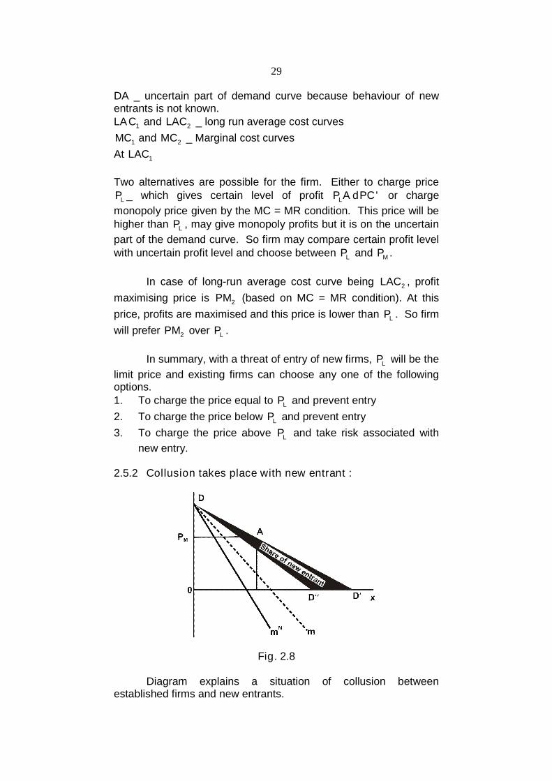
2.5.2 Collusion takes place with new entrant :

Fig. 2.8

Diagram explains a situation of collusion betweenestablished firms and new entrants.

30

DD' _ demand curveDD" _ demand curve after allocating a share of profit to newentrant at each price

New demand curve is a certain demand curve as there is acollusion with the new entrants.

There are three options.

1. Charge LP , or limit price and utilise AD' portion of the demand

curve without the entry of new firms. (As explained in the earliermodel)

2. Charge price above limit price and move on to DD” demandcurve with collusion with the new entrants.

3. Charge monopoly price MP if M LP CP (As explained in the earlier

model)

Thus, Bain’s model of limit pricing takes into account thethreat of new entrants. The existing firms may either call acceptcollusion with the new entrants or go for profit maximisation.

2.6 SUMMARY :

1. Monopolistic competition is a market structure having blend offeatures of monopoly and perfect competition.

2. Chamberlin provided for a detailed analysis of equilibriumconditions of firm and industry under this kind of a market. Heintroduced a concept of “Group” in which there are firmsproducing close substitutes or products with differentiation.

3. In the ‘Large Group’ model of Chamberlin, due to entry of newfirms in the group, a stable equilibrium with normal profitsituation can be achieved.

4. Price competition among existing firms under Chamberlin’smodel leads to adjustment process and the end result of thisprocess is a stable equilibrium with normal profit.

5. In a small group model, Chamberlin has explained how both thefirms enjoy supernormal profit by taking into consideration thecompetitor’s reaction.

6. The kinked demand curve model explain price rigidity underoligopoly.

7. All the earlier models of oligopoly do not consider the threatfrom potential entry of new firms. Bain, through his limit pricingmodel, has explained the equilibrium situation of oligopolisticfirms with new entrants.

31

2.7 QUESTIONS :

1. Explain Sweezy’s kinked demand curve model of oligopoly.How does it explain price rigidity under oligopoly?

2. What are different types of price leadership models underoligopoly? Explain output determination where leadership is bythe dominant firm.

3. What is meant by price rigidity? Why are prices rigid underoligopoly? Using the technique of kinked demand curvesexplain price rigidity.

4. Explain Chamberlin’s concept of group. How does the ‘groupattain equilibrium.

5. What is ‘Limit Price’? Explain Bain’s theory of limit pricing.

6. Write short notes on.

a) Dominant Firm Model

b) Bain’s Limit Pricing

c) Chamberlin’s Large Group’ Model

d) Kinked Demand Curve Hypothesis.

32

3

MANAGERIAL THEORIES OF FIRM

Unit Structure

3.0 Objectives

3.1 Introduction

3.2 Baumol’s Sales Maximisation Model

3.3 Morris’s Managerial Theory of Firm

3.4 Conclusion

3.5 Summary

3.6 Questions

3.0 OBJECTIVES

To understand the origin and importance of managerialtheories of firm

To evaluate the sales Maximization Model by Baumol.

To understand how growth rate miximisation is achieved asa long-term objective of a firm through ‘Marris’ Model.

3.1 INTRODUCTION

Traditionally, profit maximization has been an importantobjective of a firm. But over years alongwith profit maximizationobjective, some other objectives like maximization of salesmaximisation of growth rate have also gained importance. Thereahs been a bifurcation of ownership and management of a firm dueto complex nature of business activity in the recent years. Newtheories of firm take into consideration the role of managers indetermination of price and quantity. In the modern businessstructure, ownership lies in the hands of shareholders who arelarge in numbers. They have a power of appointing the board ofdirectors who in turn select the top management. It is the topmanagement that is involved in daily operations of the firm. Share-holders, who are the owners of a company, are the risk bearers andare interested in profit maximization by the firm. Managers, on theother hand are hired on a fixed salary and hence they may pursuethe goal of maximizing their own utility or maximizing sales(because many times managers’ perks are attached to sales)

33

Profit of course is an important determinant of all activities ofa firm, Managers’ and other stake holders job security isendangered if the firm is not making profit. But in the new pattern ofbusiness, where ownership and management are handled by twodifferent groups of people, profit maximization has no moreremained the only important objective.

Managerial Theories of firm consider the fact that themanagers maximize their utility subject to minimum profitconstraint. In this unit, we will learn three models of managerialtheory of firm – Baumol and Marris.

3.2 BUMOL’S SALES MAXIMISATION MODEL OFOLIGOPOLY FIRMS

3.2.1 Why sales Maximisation ?

As we have discussed earlier, the structure of businessorganisation has undergone transformation in the recent times. Incorporate form of organisation, Mangers dominate in the entiredecision making process of business. In such a situation, accordingto W. J. Baumol, an American Economist, Sales maximizationseems to the more realistic assumption in comparison with theprofit maximization. Baumol advocates sales maximization as anobjective of firm under following grounds :

1) Modern firms have separated the managerial functions awayfrom the ownership. In other words, owners of the firm neednot be managing the day to day activities of a firm.

2) Mangers generally pursue maximization of sales, than profitas their earnings are more closely linked with sales thanprofit.

3) Raising of funds from banks become easier for the firms withlarge size and growing sales.

4) Employees can be given better salaries and parts whensales are rising

5) Firm can be more competitive or can survive better incompetition when its sales are rising.

Baumol, however, did not ignore profits. His theory aims atsales maximisation under the condition of minimum profit. In otherwords, minimum level of profit must be earned by the managerpursuing the sales maximisation goal to ensure future growth of afirm and confidence of share holders. It is worth noting Baumol’swords.

“My hypothesis then is that oligopolists typically seek tomaximize their sales subject to a minimum profit constraint. The

34

determination of the minimum just acceptable profits level is amajor analytical problem and I shall only suggest here that it isdetermined by long-term considerations. Profits must be highenough to provide the retained earnings needed to finance currentexpansion plants and dividends sufficient to make future issue ofstocks attractive to potential purchasers. In other words the firm willaim for the stream of profits which allows for the financing ofmaximum long-run sales. The business jargon for this is thatmanagement seeks to retain earnings in sufficient magnitude totake advantage of all reasonably safe opportunities for growth andtwo provide a fair return to share holders. (W. J. Baumol, “OnTheory of Oligopoly Economical, New Series, Vol. 25, 1958)

3.2.2 Oligopoly and interdependence of firms

You are aware that one of the important characteristics ofoligopoly is interdependence of firms. Under oligopoly, there are afew firms and they are interdependent on each other, they have tothink about the reaction of their competitors while taking anydecision about price and quantity changes of their product.According to Baumol, oligopolistic firms, in their day to dayoperations, need not worry about the competitor’s reaction. In otherwords, firms daily decisions are taken on the premise that these willnot bring about changes in the behaviour of competition firms.However, the reaction of competitors becomes more importantwhen oligopolistic firm takes some radical decision like launchingnew product or advertising campaign etc. Thus the mangers willignore the competitors to the extent that their actions do notencroach on the firm’s market and do not interfere with the desiredgrowth rate and market share of a firm.

Baumol’s model is based on the following basic assumptions

1) It s a single period analysis

2) During this period firm aims at maximizing total salesrevenue (and not physical quantity of output under minimumprofit constraint)

3) Minimum profit level is determined exogenously by thedemands and expectations of shareholders, banks andfinancial institutions.

4) Conventional cost analysis based on ‘U-shaped’ cost curveis assumed under this model

Based on these models we will understand three differentmodels described by Baumol :-

1) Single product without advertising

2) Single product with advertising

3) Multiple products without advertising3.2.3 Single product without advertising

35

We first explain Baumol’s model for a firm which produces asingle product and does not incur any advertising expenditure. It isnecessary to understand following diagram to explain price –quantity determination under this model.

Figure 3.1

In the diagramTR – Total Revenue curve for the firmTP – Total Profit curve for the firmTC – Total Cost curveML – Minimum level of profit which the firm must earn.

Total profit is a different between total cost and total revenueof a firm.

We will first understand how a firm determines quantity andprice with the objective of profit maximization. Since profit is adifference between total cost and total revenue, maximum profit willbe at that point where the vertical distance between TR and TC ismaximum or where the TP curve reaches to its (highest) level. Sounder profit maximisation objective firm will produce “OA” level ofoutput because that level of output corresponds to the highest pointon TP curve (Point H).

Next to understand is the situation in which a firm would aimat sales maximization in the diagram; sales are maximized at thelevel of output OC, which corresponds to highest revenue R.

As per the assumption of Baumol’s model a sales revenuemaximizing firm has a minimum profit constraint. In other words,even if the firm is maximizing sales revenue, it has to do so underthe conditions of minimum profit level AT “OC” level of output even

36

though the sales are maximized minimum profit level (ML) is notreached. At “OC” level of output profit level is less than ML. So thisis not what Baumol has contented.

Equilibrium price and quantity under oligopoly with salesmaximisation subject to minimum profit constraints is at the outputlevel OB.

It should be noted that under Baumol’s model of oligopolyfirm, sales revenue maximisation leads to more quantity at lowerprice as compared to profit maximisation situation.

3.2.4 A single product model with advertising

Under oligopoly, firms compete not only in terms of price butalso in terms of advertising expenditure, product changes, aftersales services etc. Baumol presented another version of salesmaximisation model with advertising as one of the policy variables.An important assumption of this model is that advertisingexpenditure will always shift demand curve to the right indicatingthat the firm will be able to sell more and get larger revenue afteradvertising expenditure. Following diagram explains this version ofBaumol’s model.

Figures 3.2As per the diagram advertising expenditure is shown on the

x-axis and total cost total revenue and total profit is shown on the y-axis. As stated earlier according to Baumol, increase in advertisingoutlay will lead to increase in sales of the firm (sometimes atdiminishing rate) Increase in the physical volume of sales leads toincrease in the total revenue of the same firmTR – total RevenueOD – advertising cost

37

Production costs (fixed and variable costs) are shownindependent of advertising expenditure. So by adding fixed cost(OT) to the advertising cost curve OD we get total cost curve TC.Difference between TR and TC is profit ThereforePP – Total profit curve

Profit maximizing output level will be produced with

advertising expenditure equal to OA1, (because at that level thetotal profit is highest)

Revenue maximizing output level will be reached with

advertising expenditure equal to OA2, (Where the firm maximizesits total revenue with minimum profit constraint)

As seen in the diagram OA2 is greater than OA

It may be, hence concluded that in order to maximize saleswith minimum profit. Constraint greater level of advertisingexpenses are to be incurred by the firm as compared to advertisingexpenses of profit maximizing firm.

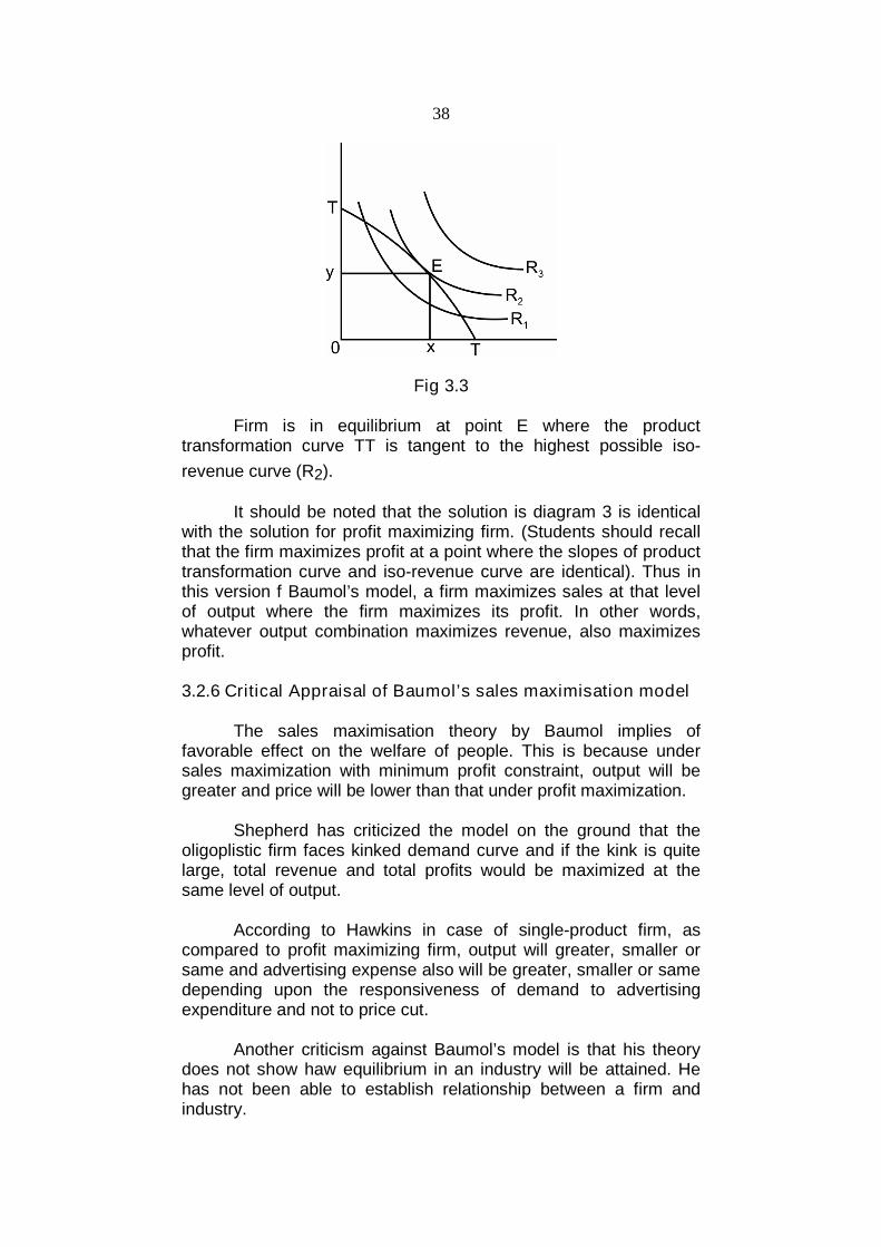
3.2.5 Multi product firm without advertising

This version of model explained by Baumol is based on theassumptions such as

1) Costs are given2) Firm produces two commodities and Y

To explain the equilibrium condition of a firm aiming at salesmaximisation with multiple products and without advertisingexpenses, Baumol has made use of two apparatus

1) Transformation curve or marginal rate of producttransformation, which is a ratio of marginal costs of twocommodities x and y. Product transformation curve isconcave to the origin showing increasing cost of reducingone product (say y) and reallocating the resource to produceother commodity (say x)

2) The iso-revenue curve is the curve showing same revenueearned by different combinations of x and y. Higher the iso-revenue curve higher will be the total revenue earned.

Following diagram shows equilibrium of multiproduct firmwithout advertising.

38

Fig 3.3

Firm is in equilibrium at point E where the producttransformation curve TT is tangent to the highest possible iso-

revenue curve (R2).

It should be noted that the solution is diagram 3 is identicalwith the solution for profit maximizing firm. (Students should recallthat the firm maximizes profit at a point where the slopes of producttransformation curve and iso-revenue curve are identical). Thus inthis version f Baumol’s model, a firm maximizes sales at that levelof output where the firm maximizes its profit. In other words,whatever output combination maximizes revenue, also maximizesprofit.

3.2.6 Critical Appraisal of Baumol’s sales maximisation model

The sales maximisation theory by Baumol implies offavorable effect on the welfare of people. This is because undersales maximization with minimum profit constraint, output will begreater and price will be lower than that under profit maximization.

Shepherd has criticized the model on the ground that theoligoplistic firm faces kinked demand curve and if the kink is quitelarge, total revenue and total profits would be maximized at thesame level of output.

According to Hawkins in case of single-product firm, ascompared to profit maximizing firm, output will greater, smaller orsame and advertising expense also will be greater, smaller or samedepending upon the responsiveness of demand to advertisingexpenditure and not to price cut.

Another criticism against Baumol’s model is that his theorydoes not show haw equilibrium in an industry will be attained. Hehas not been able to establish relationship between a firm andindustry.

39

3.3 MORRIS’S MANAGERIAL THEORY OF FIRM

Another new theory, stressing the role of managers and theirbehavioural pattern in determining output and price of firm was putforward by Marris. According to him, Managers do not aim atmaximizing profits but they seek to maximize balanced growth rateof a firm Maximisation of balanced growth rate means maximizingthe rate of growth of demand for the products of firm and the rate ofgrowth of capital supply

Maximise g = gD = gc

Whereg = balanced growth rate

gD = growth of demand for product of a firm

gc = growth of supply of capital

While maximizing growth rate, there are two constraintsfaced by the manager of a firm :-1) Managerial constraints2) Finanacial Constraints

Managerial constraints are set by the available managerialteam and its skill. Financial constraints are set by desire ofmanagers to achieve maximum job security. It is important to notehere that the managers aim of maximizing rate of growth ofdemand to maximize their own utility and they aim at maximisationof growth of capital to maximize the utility of owners andshareholders.

3.2.1 Manger’s utility Function

Manger’s utility function includes the variables like salaries,status, powers and job security. Owners’ utility function includesvariables like profits, size of output, size of capital, share of marketand public image. Thus, due to division of management andownership has resulted in setting goals which may not necessarilycoincide.

Um = f(salaries, power, status, job security) This is mangersutility function.

3.3.2. Utility function

Uo = f* (profits, capital, output, market share, public esteem) This is owners’ utility function

The managers aims at maximizing utility as per Um functionand the owners’ aim at maximizing Uo function. According to

40

Marris, the difference between these two functions is not widebecause most of the variables are strongly correlated with eachother. Marris believes that the size of a firm may be measured bythe level of output, capital supply, sales revenue and market share.Achieving steady balanced growth implies the growth of most of thevariable occurring in above mentioned functions such as sales,output, supply of capital etc. Marris further argues that themaximization of growth rate of firm is compatible with the interests

of share holders. So growth of demand/output of a firm. (gn) and

growth of capital supply (gc) of a firm need not be differentiated. Inother words, when the rate of growth of firm is higher, manger’ssalaries will be higher they will have power and more job security.So mangers’ utility function can be written as

UM = f(gD, S)

Where gD - growth of demandS – measure of job security

On the other hand, owner’s utility depends upon the growth ofcapital supply. So his utility function can be written as

UO = f* (gc)

Following E Penrose’s “Theory of Growth of firm” Marris

argued that gD or growth of demand for product is constrained bydecision making capacity of a manager Job Security S isdetermined by three financial indicators

1) Liquidity Ratio2) Debt. Asset. Ratio and3) Profit Retention Ratio

Marris’s treats ‘s’ as an exogenously determined constraintin the managerial utility function. Taking this factor intoconsideration manager’s utility function may be rewritten as

UM = f(gD)s

Where s is a security constraint.

3.3.3. Constraints in the Model

As discussed in the earlier part of the theory, thee are twoconstraints in the model.

The Managerial constraint andThe Job security constraint

Since the decision making and planning of firm’s operationare the result of team work of managers, the efficiency of top

41

management acts as the managerial constraint in the model.Research and Development (R & D) department also set limit to the

rate of growth of firm. Thus, both gD and gc have managerialconstraint.

The job security constraint makes managers become risk-avoiders by choosing steady performance and not risky ventureswhich may be highly profitable. Managers also prefer prudentfinancial policies by determining optimum levels for the threefinancial ratios mentioned in the earlier section :- Liquidity Ratio,Debt ratio, and Retention Ratio. These three financial ratios arecombined into a single parameter a which is called ‘financialsecurity constraint’. It is exogenously determined by the topmanagement.

According to Marris, two ponts need to be stressedregarding the overall financial constraint a .

a1 = Liquidity RatioL Liquid Assets

A Total Assets

a2 = Debt RatioD Value of Debt

A Total Assets

a3 = Retention Ratio R Re tained profit

Total

Profit

1) Overall a is negatively related to a, and positively related to

a2 and a3.2) There is a negative relationship between job security (s) and

financial constraints (a )

3.3.4 Equilibrium of a firmManagers aim at maximisation of their own utility

UM = f(gD)Owners aim at maximisation of their own utility

UO = f*(gc)Firm is in equilibrium when

gD = gc = g* maximum

where g* is maximum balanced growth rate gD will dependupon the rate of diversification or introduction of new products (d)and the proportion of successful new products (k) which in turn willdepend upon price of product (p), advertising expenditure (A) andexpenditure on Research and Development (R & D), Thus

gD = f(d, k)

gc (Rate of growth of capital supply) will depend upon themagnitude of profit

gc = f() = profits

42

According to Marris, further, growth rate of supply of capitaldepends upon average rate of profits (m) which is obtained bydeducting cost per unit, advertising expenditure per unit and R & Dexpense per unit from the price of product

m = p – c (A) – (R & D)

Growth rate of capital supply also depends upon the rate ofdiversification (d). So

= f(m, d)

Substituting this profit function the in the function governingsupply of capital, we have

gc = a ()Where a is financial security constraints

As long as financial security constraint is constant, growth ofcapital and magnitude of profit are not competing goals. Higherlevels of profits means the higher growth of capital supply.

Given the above function related to rate of growth of demandfor product and the rate of growth of capital supply, the firm will bein equilibrium when it is achieving the highest rate of balancedgrowth

gD = gc = g* maximum

3.3.5 Evaluation of Marris’s Model

The most important contribution of Marri’s model ofmanagerial theory of firm is the inclusion of financial policies of thefirm into the decision-making process. The financial constraintcoefficient a plays a very important role in the entire model as apolicy variable. However, the model actually does not say muchabout the value of a . It is assumed to be exogenously determined.

According to the conclusion of the model balanced growthsolution will maximize the utility functions of both mangers andowners. But it may be so during the periods of steady growth andnot during recessions or tight markets.

One of the implications of the model is that both the mangersand owners prefer maximization of rate of growth over themaximization of profits. Marris does not justify the preference ofowners for capital growth over the maximisation of profits.

The model assumes price and cost to be constant. It fails totake into consideration the interdependence of firms under theoligopolstic structure.

43

Further, the model assumes a continuous growth by cratingnew product. But it fails to realize that new products may beimitated by the rivals and this, in the longrun will hinder the steadygrowth of firm.

There are many restrictive assumption on which the Marrismodel heavily relies. Such as each firm has its own R & Ddepartment, R & D and advertising expenses together influence thegrowth rate of capital supply etc.

3.4 CONCLUSION

In conclusion it may be observed that managerial theories offirm in general fail to explain the oligopolistic structure of market.These theories are excessively dependent on the assumption ofunlimited power of firms to influence market through advertisingand introduction of new products. These theories also fail to explainthe price determination pricess in the oligoplistic market.

3.5 SUMMARY

1) In addition to traditional profit maximisation as an objective firm,many other objectives such as sales maximisation growthmaximisation etc. have been put forward in the recent years.

2) Due to bifurcation of management and ownership function of afirm, sales maximisation has become important objective,according to Baumol.

3) Though Baumol stresses on the sales maximisation objective ofthe firm, minimum profit constaint plays important role in hisanalysis.

4) According to Marris, long run growth rate maximisation is anobjective of a firm. Maximisation of rate of growth of demand forthe products of the firm and the rate of growth of capital supply,would bring about maximisation of balanced growth rate.

3.6 QUESTIONS

1) Discuss the importance of managerial theories of firm.

2) Critically evaluate Baumol’s sales maximisation model.

3) Explain Marris’s Growth maximisation model.

44

4

Module 2

INVESTMENT DECISIONS

Unit structure :

4.0 Objectives

4.1 Introduction

4.2 Investment decision Capital appraisal-methods

4.3 Risk and Uncertainty

4.4 Sensitivity analysis

4.5 Financial statements

4.6 Summary

4.7 Questions

4.0 OBJECTIVES:

To understand risk involved project selection To understand various methods of project appraisal and

investment decisions To know what is risk and uncertainty To understand the relevance of sensitivity analysis To know about financial statements and its components

4.1 INTRODUCTION:

Every industry or company wants to grow and expand itsbusiness locally and globally. Need always arises to expand theoperation through branches or new set up. Most of the companiesexpand their business by investing in new projects. However it isnot a sudden decision they make but it needs proper evaluation ofprojects and their viability of success. So the terms like capitalbudgeting and sensitivity analysis are common in this regards. Inthis module we are going to study about the investment decisionstaken in the industry or company while selecting project forbusiness development. Module will focus on investment relatedterms and finance. Company maintains accounts and financialstatements to know the profits and operational efficiency. They

45

compare their profits with other concerns or for years for selfconcern progress indications. This module discusses about the riskand uncertainties prevailing in project selection and sensitivity inmaking investment decision accordingly.

4.2 INVESTMENT DECISION AND PROJECTAPPRAISAL METHODS

There are many methods of appraising the projects. Beforetaking capital investment decision it is necessary to do a projectplanning. Project planning starts with the exploration of a businessopportunity. In this detailed investigation is made of differentaspects such a managerial, technical, marketing, economics,operational and financial toward the project acceptance. Afterevaluating the project, a report is made known as project report. Itis a real blue print on which basis the project gets a concreteshape. It has importance because every firm intends to maximizeits profit.

Investment decisions are based on the evaluation of suchprojects living scope for capital budgting. Capital investment isconcerned with comparing the benefits that accrue over a period oftime with amount invested. Therefore all the project proposals haveto be ranked in the order of preference yielding maximum returns. Itis absolutely necessary to evaluate the projects before makinginvestments.

There are three methods of appraising projects:

4.2.1. Pay-back method:

The most simple and widely accepted of project evaluation ispay-back period or pay-out or pay-off period. By this method it iscalculated that within what time the investment done is recovered inthe form of annual cash flows. In simple language, it is the period ornumber of years required to recover the original cash outlayinvested in a project. This method is also known as cash-to-cash tomethod. every project generates annual cash flows. Therefore it isseen which project investment amount is recovered soon andaccordingly that projects is ranked first.

The formula used in this calculation is :

Pay-back period = Total Investment outlays/Annual cash flow.

Merits: It is simple and easy method of evaluating and ranking projects.

It is more concrete and realistic.

46

It problem of liquidity is easen as it considers the annual andregular recovery of cash flow.

Risk can be minimized by selecting most beneficial project first. This method is widely used in industries for project evaluation. This methods is used for short terms as well as long term

investment projects. It is suitable when firm is in urgency of cash realization.

Limitations: It stresses on only one aspect more that is of liquidity. Long term projects cannot be evaluated by this method

properly. Consistent cash flow is assumed in this method so change is

cash flow is not considered in this method Time value of money is not considered in this type of method. Sales promotion techniques are not considered in this methods

being the most cash realizing factor those are adding to cashinflows.

4.2.2 Net present Value method :

In this method, the investors take investment dictions on thebasis of net present value. It is also known as discounted presentvalue method. Here the fact is considered that the amount ofmoney received today is more valuable that the one received afteryear or years. The intention behind is that the money receivedtoday can be invested to earn certain amount of interest. Thepresent value of an investment proposal is the difference betweenthe total of present values of the estimated annual cash flows overthe life of the project and initial investment of the project.

NPV is difference between discounted value of all the net cashflows and capital cost of the project.

Decisions with consideration of NPV is taken on the basis offollowing rules:

If NPV is positive, the project will be acceptedIf NPV is negative, the project is rejectedIf NPV is zero, there will be indifference in selecting the project inthe choice.

Merits: It takes into consideration income derived from capital over the

entire life time For many projects this method is useful Time value of money is highly considered in this method It is widely used and popular method of project evaluation

47

If number of investment proposals are to be considered thefollowing formula is used:

NPV indeed = Total present valued of all cash flows----------------------------------------------Initial investment made

Demerits: If the rate of investment is to be considered over the investment,

then it is absolute method. It is more subjective, lengthy and complex method as compared

to pay back method of project evaluation.

4.2.3 Internal rate of return (IRR) method:

Under this method, time factor and opportunity cost ofinvestment is considered. It is same like MEC method given byKeynes. MEC stands for Marginal Efficiency of Capital. Thismethod is based on the technique of discounting cash flow. It is thediscount rate which equates the discounted present value of itsexpected future marginal yields with the investment cost of project.IRR is the annual expected rate of profit over the life of the machinefrom the investment in a project. It is the rate of discount whichequates the present value of the income stream over the life of themachine with the net cash investment.

The rate of return calculation that takes into account the timevalue of money is called discounted cash flow method.

Trial and error procedure has to be employed in finding outthe internal rate of return because cash benefits consists of anuneven series. If the IRR exceeds the market rate ofinvestment(cost of capital), such a project is accepted.

Merits: It recognizes time value of money It considers whole annual returns earned during the lifetime of

the project Decisions are most polished.

Demerits: It is difficult and complex method. It is lengthy procedure and not easy to calculate Projects having different investment costs can never be ranks

properly by this method. It is more objective because the IRR is not directly influenced by

decisions regarding depreciation methods, capitalization versusexpenses decisions and conservatism.

48

PRACTICAL SUMS SOLVED

From the information below calculate:i)Pay Back Periodii)Pay Back Profitability

Particular Model A Rs. Model B Rs.

Investment 5,00,000 7,50,000

Estimate Life ( in years) 10 10

Sales 10,00,000 20,00,000

Direct materials 4,00,000 6,00,000

Direct Labour 1,20,000 2,00,000

Cash Overheads 1,60,000 2,40,000

Depreciation 50,000 75,000

Solution:

Calculation of Labour Inflow

Particular Model A Rs. Model B Rs.

Sales(I)

10,00,000

Less: Variable Cost

Material 4,00,000 6,00,000

Labour 1,20,000 2,00,000

CashOverheads

1,60,000 2,40,000

6,80,000 10,40,000

Contribution(I-II)(II)

3,20,000 9,60,000

Less: Depreciation 50,000 75,000

P.B. Tax 2,70,000 8,85,000

Less: Tax -- --

P.A. Tax 2,70,000 8,85,000

Add: Depreciation 50,000 75,000

3,20,000 9,60,000

49

i) PaybackPeriod

A B

= =

= 1.5625 years = 0.78125 year

ii) PaybackProfitability

=3,20,000 *10 =32,00,000 96,00,000

Less: Cost =5,00,000 7,50,000

=27,00,000 =88,50,000

Q 2. Base Line Ltd; has a machine which has been in operatingsince 6 years. The management is considering a proposal topurchase an improved model of a similar machine which will givean increased output. You are given the following information.

Particular Old Machine Rs New Machine Rs

Cost of Machine 8,00,000 20,00,000

Variable cost perunit

300 300

Fixed overheadsexcludingdepreciation

2,00,000 4,00,000

Selling price per unit 600 600

Output 1,500 Units 2,500 Units

The Life of both the machine is 10 years each. Depreciation bySLM. Tax rate 50%. Calculate PB period and paybackprofitability.

Solution:

Calculation of cash Inflow

Particular Old Machine Rs. New Machine Rs.

Selling Price 600 600

Less: Variable Cost 300 300

Contribution 300 300

Output ( Units) 1,500 2,500

Contribution 4,50,000 7,50,000

50

Less: Fixed cost 2,00,000 4,00,000

PBD & Tax 2,50,000 3,50,000

Less: Depreciation

( )

80,000 2,00,000

Profit before Tax 1,70,000 1,50,000

Less: Tax 50% 85,000 75,000

Profit after Tax 85,000 75,000

Add: Depreciation 80,000 2,00,000

CASH IN FLOW 1,65,000 2,75,000

i)Pay back period= 8,00,000 20,00,000

4.8484 years 7.2727 years

ii)Payback Profitability =Inflow * No of Years

16,50,000 22,75,000

Less: Investment 8,00,000 20,00,000

=8,50,000 2,75,000

Q3 Following is the relevant data for two machines A & B.

Particular A Rs. B Rs.

Capital Outlay 2,000 2,400

Net Cash Flow

1st Year 1,000 800

2nd Year 1,000 800

3rd Year Nil 2,000

Find out which of the two is a better investment, showingworkings. Use Pay – Back Period.

Solution:

(A)Pay – Back Period Method

Particular Machine

A B

Pay – Back Period 2 years 2 years + i.e.,2

Machine A is a better investment, as it has a lower Pay – Backperiod.

51

(B) Post Pay – back Profitability Method:

Post – Payback Profitability = Total Savings – Capital Outlay.Machine A = 2,000 – 2,000 = NilMachine B = 3,600 – 2,400 = Rs. 1,200In this case Machine ‘B’ is a better investment.

Illustration 10

Shobhit ltd; is considering to purchase a machine. Two MachinesA and B available at the cost of Rs. 1,20,000 each. Earnings aftertax but before depreciation are likely to be under:

Year Machine ARs.

Machine BRs.

1 50,000 20,000

2 40,000 30,000

3 30,000 50,000

4 20,000 40,000

5 20,000 40,000

Evaluate the two alternatives by using:(1) Pay – Back period method

Solution:

(1)Calculation of pay – back period:

Year Machine A Machine B

C.I Cum. C.I. C.I. Cum. C.I.

1 50,000 50,000 20,000 20,000

2 40,000 90,000 30,000 50,000

3 30,000 1,20,000 50,000 1,00,000

4 -- -- 40,000 1,40,000

C.I. = cash Inflow.P.B.P. Machine A = 3 yearsP.B.P. Machine B = 3 years + years 6 months

Ans:As recovery of investment done on machine A is early of 3 years itis preferable to invest in the same.

4.3 RISK AND UNCERTAINTY

Risk and uncertainty has been the inseparable part ofbusiness activities or investment decisions. Only difference in both

52

is that risk can be insured while uncertainties are true risk whichmay make suffer or prove harmful for business.

According to the Oxford dictionary definition of risk “thepossibilities of meeting danger or of suffering harm or loss.” Thereare many kinds of risks observed in investment they are

Business and financial risk:They are actually two separate type of risks but are

interrelated too. Business risk is also known as operating risk and isassociated with day to day operations of the business. While,financial risk is the risk created by debt and preference shares andsecurities. These risks are dependent or caused upon competition,new technologies, change in consumer preference, governmentpolicies and poor performance of business.

Interest rate risk:It is another risk. It occurs due to change in interest rates of

securities. It happens due to speculations.

Market risk:This kind of risk arises due to the change in psychology of theinvestors, unexpected war conditions, political instability,speculation etc.

4.4 SENSITIVITY ANALYSIS

Risk has been the matter of profitability in the business.Without risk, profit cannot be expected. In fact, profits is the rewardfor risk undertaking. Every project undertaken has to be evaluatedfrom the point of its profitability therefore the sensitivity analysis hasa scope and relevancy in the industrial capital budgeting andinvestment decision making. Starting new project always has moreuncertainties than expanding the existing one. Therefore withreference to capital budgeting, results may vary from estimated toactual terms. The greater the variability between the two, morerisky is the project. Therefore the measure which expresses the riskin more precise terms is sensitivity analysis.

Sensitivity analysis is a behavioral approach that uses anumber of possible values for a given variable to assess its impacton a firms returns. In the area of finance, such kind of analysis isrelated with capital budgeting decisions.

It focus light on the sensitivity of the project in respect itsexpected cash flow, the discount rate. It is very important becausethe future is uncertain and nothing can be estimated perfectly aserrors are ought to happen all the time. Therefore this kind of

53

analysis leaves scope for the project evaluation in the bettermanner. The viability of outcome is estimated with expected cashinflow and decisions are taken accordingly. The various estimatesare made regarding cash flow estimates under three assumptionsthe worst (most Pessimistic), the expected (the most likely) and thebest (the most profitable).

Significance of sensitivity analysis: It ensures the benefits to be derived from the chosen project. It considers terms of risk and uncertainty to ensure project

viability It ensure more than one estimate of the future return of a

project. It gives precise idea about project viability and makes easy its

selection It expands the study of increasing returns and wise investments.

4.5 FINANCIAL STATEMENT

Financial statements are the financial reports referring twostatements reflecting assets and liabilities of the company. Theyare very important in accounting and corporate reporting. Theysupport whole accounting system. They are balance sheet andprofit and loss a/c. balance sheet represents capital, assets andliabilities of the company and Profit and Loss a/c indicates theresults of operations of the company during a given period of time.They are summary of accounting transactions. They are neededand prepared for reviewing periodic progress of the company.Financial statements are prepared in a certain format by followingcertain rules. It facilitates the users to compare different companiesand their financial performance.

Components of financial statements:

Profit and loss account :

It is also called as ‘Income statement’. It indicates theamount of net income or loss obtained by the company during aparticular period. Net income in excess of revenue over itsexpenses. It is the best measure to assess the profitability andperformance of the company.

Balance Sheet :

It is also called as ‘statement of Financial Position’. Itrepresents financial position of a company on particular date. Acompany can obtain finance from owners and outsiders. Thus the

54

balance sheet three major sections viz assets, liabilities andshareholder’s equity. The fundamental accounting equation of:

Assets = Liabilities +Equity

Characteristics:

They are generally report prepared on the basis of theaccounting transactions taken place already. They never dealwith the future operation estimations.

They are the summarized reports of the whole businesstransaction taken place during a give period of time. It alsoclassified items accordingly.

Most of the financial statements are prepared on accrue basisrather than on cash basis. Expenses due but not paid andincome due but not received are mentioned.

It has the blending of economic and legal aspects. Conventionsare followed while preparing these statements.

Most of the time, these statements are based on the estimates,personal opinions and judgments.

These statements are based on the reliable facts andverification. So there are less chances of false or faketransaction.

Financial statements are interrelated the for they are said to be‘Articulated’

The base of preparing financial statement is monetarytransactions. Without cash transactions these statements areuseless.

IMPORTANCE/ SIGNIFICANCE/ ROLE/NEED FINANCIALSTATEMENTS

Communication:The main purpose of these statements is to communicate

with the interested parties. This helps in making economicdecisions. Statements are prepared for letting know thestakeholders about the operations and economic activities carriedby the company.

a) Bankers.Banks before granting loans to the corporate and companies

takes into consideration the progress of the company through theirfinancial statements. The come to know the profitability, solvency,liquidity of the company.

55

b) Shareholders:Being the owner of the company, shareholders always are

interested to know the financial statements of the company to knowthe progress and value of appreciation of their shares invested inthe company.

c) Lenders:banks, financial institutions and other lenders of funds to the

business entity also wish to know the profitability and liquidityposition of the of the company whome they lend. It provides somekind of assurance to them of their returns.

d) Suppliers:Suppliers of the company are interested to know the short

term liquidity of the company. It decides the credit rating status ofthe company. These statements helps them to ascertain thecapacity of the organization to pay them on time for the goods andservices supplied.

e) Employees:Most of the incentives policies of the company depends

upon the profitability of the company, so employees are alwayscurious to know the profitability of the company. This they come toknow from the financial status of these statements.

f) Government:Financial statements helps government to decide the correct

tax and duties to be levied on the industries. Therefore the taxpayable by the enterprise is dependent on the financial statementsof the company.

g) Information:Financial statements are prepared for the showing changes

in economic resources. It helps in revealing reliable information toall, who are concerned with the progress of the company.

h) Prediction:Financial statements are prepared in a way to provide

information that is useful in predicting the future earning power ofthe enterprise or industry.

i) For reliability:FS are prepared to provide reliable information about the

earnings of the business enterprise and its ability to operate at aprofit in future. This helps the above stakeholders to trust themanagement or organization.

56

Q Characteristics/good essentials of financial statements:

a) Understandability:Information provided in the financial statements must be

readily understandable and comprehend. It does not mean thatcomplex information should be excluded. But it has to be presentedto comprehend or understand easily.

b) Reliability :Information provided in the statements should be reliable.

Reliability means faithful information which is presented. Thereshould not be error, bias. It must be complete within the limits ofmateriality of cost.

c) Relevance:When the information of financial statement is useful for

decision making, then it is said to have relevancy. Information issaid to be materialistic if its omission or misstatements couldinfluence the economic decision of users.

d) Comparability:The statements should be comparable across companies to

make resource allocation decisions. Trends of statements shouldbe comparable over the period of time to know the progress of thecompany. Lack of consistency threatens the comparability of thefinancial statements.

Check Your Progress :

1. Bring out difference between Risk and Uncertainties

2. What do you mean by capital budgeting?

3. What are the methods project evaluation and investmentdecision making?

4. What do you mean by Financial statements and what are themajor components of it?

5. Why sensitivity analysis is necessary? Give reasons for it.

57

4.6 SUMMARY

1. Investment and capital budgeting is done by companies whenthey need to chose new project for expansion purpose. Thesedecisions are very sensitive because they may result in profit ormay lead to loss.

2. Risk and Uncertainty has been the integral part of businesswhich makes it to earn profit. Risk is expected and so can beinsured but Uncertainties are situational and cannot be insuredand are truly called risk.

3. Many methods are used for selecting project on the basis theperiod within which it covers the investment made and earningcapacity. Pay-back, IRR and NPV methods are most commonmethod being used by companies for making investmentdecision out of many proposals available.

4. Companies keep record of their operations in the form offinancial statement like Profit and Loss analysis and balancesheet focuses on total assets and liabilities held by the companyand the operational profit and loss incurred.

4.7 QUESTIONS:

1. What do you mean by capital budgeting and what are thevarious methods of project evaluation?

2. What are the conventional and modern methods of investmentdecisions?

3. Explain terms Risk, Uncertainty and Risk sensitivity analysis.

4. What do you mean by financial statements? Explain itscharacteristics, components and significance in brief ?

58

5

RATIO ANALYSIS

Unit structure

5.0 Objectives

5.1 Introduction

5.2 Ratio analysis

5.3 Inflation accounting

5.4 Sources of finance

5.5 Capital structure

5.6 Separation of ownership and control

5.7 Summary

5.8 Questions

5.0 OBJECTIVES

To know uses of Ratio analysis in managerial decision making

To know what is inflation accounting

To know various financial sources to raise funds

To understand what is capital structure and its principles

To understand difference between ownership and controlseparation principle.

5.1 INTRODUCTION

Last part we focused on capital budgeting and investmentdecisions to be taken by considering many methods of it. In thismodule we shall try to learn about how the profit and loss status orposition by companies by adopting tools like ratio analysis.Companies do calculate their operation numerically and find outprogress of them. Due to change in prices day by day companiesare also required to consider price fluctuations to prepare financialstatements to show real position of the companies. This is learnt byknowing term like Inflation accounting. In this module we are alsogoing to learn how companies raise finance from their internal aswell as external sources. How do they keep proportion betweenowned and borrowed capital is known by capital structure term.

59

Moreover this module also explains the difference betweenownership and management of the company.

5.2 RATIO ANALYSIS

A ratio is one figure expressed in terms of another figure. Ithas mathematical application to find out the relationship betweentwo numbers or items of the financial statements. Ratio isexpressed by dividing one figure by other related figure. It isexpressed in fraction or as pure ratio. Ratio analysis is a verypowerful tool used for measuring performance of the organization.It expresses the inter-relationship among the figures appearing inthe financial statements. It helps firm to analyze the pastperformance and carry out future projections. Ratio is expression ofone number against another. For ratio analysis various formulasare used to know the solvency, liquidity of the firm.

Ratio may be expressed in percent (40%) or proportionate ratio(4:1) or in times ( 4 times a year).

Importance:

It helps in making inter-firm comparisons among various firmsand even between the difference divisions of company.

By using trend analysis along with ratio’s helps a firm to knowthe performance of the company over the period of time.

It helps in analyzing causal relationship among different itemsby considering past results.

It throws light on the efficiency of the management beingbarometer for future.

It simplify and summarize numerous accounting data in asystematic manner so that the simplified data can be usedeffectively for analytical studies.

It helps in controlling efficiency and profitability of a businessentity.

They are yardsticks, used by all institutions in evaluating thecredit-standing of their borrowers and customers.

Departmental performances can be traced and expressed byratio analysis.

They assist investors in making sound investment decisions andalso the shareholders in evaluating the share performance.

60

Ratio statements:

Balance sheet ratios Revenue statementsratio

Composite ratios

Liquid ratio Operating ratio Return on capitalemployed

Current ratio Gross profit ratio Return on ownersfund

Properitory ratio Expenses ratio Return on equity

Capital-gearing ratio Net profit ratio Earning per share

Stock-working ratio Stock-turnover ratio Debtors turnoverratio

Classification of the ratios:

1. Liquidity Ratio:Short term and immediate financial position of a business

organization is analysed by these ratios. They indicate the ability ofthe organization to meet its short term obligation, so calledliabilities. They are also known as solvency ratios. They see theasset adequate to meet its liabilities .

2. Activity ratios:It indicates how effectively firm is using its funds. They are

so called as performance or efficiency ratios as they indicate thedegree of efficiency of the organization. It reveals operationalbehavior of the organization.

3. Leverage ratios:If measure the relationship between proprietor’s funds and

borrowed funds. They indicate companies debt and financing.

4. Profitability ratio:They reflect the over-all efficiency of the organization its

focuses light on the investment policies.

Exhibits 2.3 RATIOS – COMPUTATION AND COMMENTS

Objectives ofanalysis

Ratio to beComputed

formula

ImmediateLiquidity

Quick Ratio]

Short – termLiquidity

(A) Current Ratio ]

61

Liquidity of Stock ( B) Stock WorkingCapital

]

( C)Stock Velocity

2

Liquidity ofdebtors

(D) Debtors’Velocity

Liquidity ofcreditors

(E) CreditorsVelocity

Long – TermSolvency &stability

(A) ProprietoryRatio

(B)Debt – EquityRatio

Operating ortrading efficiency

(A)Gross ProfitRatio

* 100

(B)Operating Ratio

( c)Operating NetProfit ratio

62

(D)Expenses Ratio

(E) Net Profit Ratio

OverallProfitability

(A)Return onCapital Employed

(B)Return onProprietor’s Fund

( C)Return onEquity Capital

Capital Structure (A)Capital Gearing

(B) Debt. Equity

( c)ProprietoryRatio

Overtrading orUnder trading

(A)ProprietoryRatio

(B)Stock Turnover

( c) Current Ratio

63

Coverage (A)DividendPayout

(b)InterestCoverage

Q Limitations of ratio analysis:

It is basically historical in nature unless projected studies are tobe made.

Difference in accounting policies and accounting period makethe accounting data of two firms non-comparable.

In case of firms having diversified product lines, of differentindustries, the ratio calculated aggregately cannot be used forinter-firm comparison.

Seasonal factors may also influence financial data. As the stockmay be high or low according to festivals and seasons.

Ratios are only symptoms and not solutions.

In many situations, accountant has to make choice out ofvarious alternatives available. So subjectivity is high in thiscase.

It is quantitative in nature and not qualitative in nature.

Realities behind the prepared may be different than what ispresented in the ratios because most of the firms go for windowdressing to show their balance sheet strong.

Price level changes make ratio analysis meaningless.

5.3 INFLATION ACCOUNTING

Inflation refers to a rise in price level and fall in money valueafter full employment level has been achieved. Under suchconditions only prices will rise and output will remain the same.Inflation is a state where aggregate demand for goods and servicesexceeds aggregate supply. When aggregate demand is highermore than aggregate supply, the prices level generally increases. Ifsuch a situation persist for a long period of time, it leads to inflation.Due to change in factor prices and goods prices need is to studyinflation accounting. It is exactly opposite to historical costaccounting where changes (inflation) on income and assets arecompletely ignored.

64

Inflation accounting is also known as accounting forchanging prices. It can be defined as a system of accountingwhich regularly records all items in financial statements ate theircurrent values or changed values. It is new accountingdevelopment which studies impact of changing prices overhistorical costs. It shows inflation adjustments to the historicalfigures appearing in the books of accounts of a company. Thisaccounting do consider that due to rise in prices, purchasing powerof the consumers is decreasing day by day. Financial statementsare prepared on the basis of current prices prevailing in theeconomy.

Objectives:

To show real financial position in present day terms and to showthe real capital employed.

To make sure that sufficient funds will be available to replacethe assets when their replacement is due.

To know the real profits and loss for the year based on currentchange prices

To know profit in constant rupee keeping in view the generalchanges in prices.

To enable stakeholders and management real position ofoperations with references to price fluctuations.

Approaches of inflation accounting

Current Purchasing Power Accounting (CPPA):

Under this method the historical accounting data areadjusted on the basis of any established and approval general priceindex at a given date. It considers the changes in the value of itemsas a result of the general price level. It ignores changes in the valueof individual items. This method was recommended by EnglishInstitute of Chartered Accountants. According to them companyshould continue to prepare financial statements on historical costbasis. Under this method price level adjustments are made for allthe items of income statement and balance sheet.

Current cost accounting (CCA):

It is also known specific price level approach becausechange in the general level of prices which occur as a result ofchange in the value of the monetary unit are measured by indexnumbers. Specific price changes occur if prices of a particularassets held change irrespective of any changes in general price

65

level. This method has also been named as replacement costaccounting. In this method, historic values of items are not takeninto account; rather currency values of individual items are taken asthe basis for preparing profit and loss account and balance sheet.This method seeks to state the assets and liabilities in the balancesheets their current values.

5.4 SOURCES OF FINANCE

Industrial Finance may be required for short period or forlong period. It may be raised by investment of proprietors asownership funds or by borrowings. Finance is the blood of the firm,so it has to be managed from the own pocket or borrowed frominstitutions. The various sources of finance may be broadlyclassified as under: industrial finance is needed for long term,medium term and short term requirements:

A) LONG TERM FINANCE:

Owned funds:It includes owner’s investment as sole proprietor or partners

of a firm. In companies it is raised by issue of shares, ploughingback of profits, depreciation policy, dividend policy. Companiesraise long term finance by issuing equity shares and preferenceshares in the market. The main motive behind is that it can use themoney collected by such issues as owned capital. Equity sharecarry no fixed obligation against the returns or dividend .

1.PloughingBackofProfits

Like all individuals, companies also save a portion of theirprofits to be used to meet future needs. When the profits earned bya company, instead of being fully distributed to shareholders in theform of dividends, a portion is retained in the business as additionalcapital. Every company keeps some reserves with it to meet futurerequirement of cash or money. Whole of its profits is not distributedby the way of dividend or interest but kept aside to use as ownedfund for growth or expansion of business.

2. Borrowed Fund:

There are external sources of business. It includesborrowings from relatives and other sources by sole owners andpartners of business. Owned capital is never sufficient for thecompany. So it has to raise money from the financial institutions onthe fixed interest obligations . In companies borrowed funds includedebentures public deposits, banks, insurance companies andspecial financial institutions.

66

3. Depreciation Policy.

Depreciation is permanent decrease in the value of an assetthrough wear and tear in use or passage of time. It representspermanent fall in the market value of the asset. Therefore it isnecessary to make a provision for the replacement of andepreciated assets. So companies make provision for thedeprecation, by which every year some amount compared with totallife of the asset is shown as depreciation. The same amount isused to buy or purchase new asset after that period of time. A goodmanagement policy, provides for adequate depreciation on itsassets. Adequate depreciation charge is made with a view torecover through current earnings the original investment in theassets

4. DividendPolicy:

A good company always provides for all its liabilities beforepaying dividend to its shareholders. It is a part of a sound financialpolicy that company must try to establish a stable dividend rate. Itaffects the raising capital name of the company a lot. Dividend isthe return on money invested in shares. So it is absolutelynecessary to make polices to handle the matter of dividenddistribution.. For maintaining a stable dividend rate, themanagement is justified if does not pay dividends during the firstfew years in the case of new company which requires funds fordevelopment and financial stability.

The dividend may be paid in cash or by issue of bonusshares according to the availability of liquid assets and the extent ofunder capitalization existing in the company.

5.Reorganization

Reorganization of a company is done when it is in financialdifficulties or when it is desired to like advantage of certainfavorable conditions in the market. It is necessary to makeprofitable and efficient again. Reorganization may be internal orexternal.

Internal Reorganization: In internal reorganization the sharecapital is reorganized. A portion of capital is also cancelled to wipeout the capital losses.

External Reorganization: It takes place when a company goesinto liquidation and a new company is formed with the value ofassets and liabilities suitable adjusted. Money is realized by thisprocess.

67

B) MEDIUM TERM FINANCE:

Public deposits:Company also accept public deposits to make available

working capital for smooth operations. It is accepted for 6 month to3 years period. Companies offer good rate of interest on such adeposits because it satisfies the liquidity need of the company forthe medium term tenure.

Term loans:Loans having maturity period of one year are term loans.

They are repaid over a period of stimulated time.

Lease financing:Some financial sound companies buy or purchase plant or

equipments and give them on lease ( rental basis). It is also thesource of finance for them. The giving company is called as lessorand the firm who are given such machineries to use on rental basisare called lessee.

C) SHORT TERM FINANCE:

Trade credit:It is credit granted by the suppliers. It has duration of 15 to

90 days. It is common practice followed in business operations. It isvery flexible.

Bank credit:Banks do lend money by different methods such a cash

credit, bills discounting and overdraft facility to the current accountholders(businessmen). Bank is pioneer in granting such loans tothe firms to meet their financial needs.

5.5 CAPITAL STRUCTURE

Term capital is taken as wealth or total assets employed inthe business. Capital structure planning is done with an objective ofmaximization profit and minimizing cost of capital. Capital used bythe firm is mixed of owned and borrowed capital. So structure ofcapital has to be considered to determine which type of capitalcompany is intended to use. It answers how much should be thedebt and equity capital ratio. Capital structure deals with mixing thedebt and equity capital. One represent owned capital and otherrepresents borrowed capital. Company knows that depending uponborrowed capital more is always obligatory as it makes it to payregular interest and payments on it. While using the equity capitalcomprising investments done by shareholders is less obligatory asrisk is born by the shareholders’ themselves. The essence of

68

capital structure decision is to determine the relative proportion ofequity and debt.

Characteristics capital structure :

Profitability:The capital structure of the company should be most

advantageous. Within the limitation, maximum use of the leverageat minimum cost should be made so as to obtain maximumadvantage of trading on equity at minimum cost.

Flexibility:It should be flexible to meet the changing conditions. It

should make company possible to provide funds whenever neededto finance its profitable activities.

Control:The capital structure should involve minimum risk of loss. It

should be used for controlling risks.

Broadly speaking, there are three fundamental patterns ofcapital structure in new concern

Financing of capital requirement exclusively by equity.Financing of capital requirement by equity and preferred stocksFinancing of capital needs by equity and preferred stocks andbonds.

Principles to be considered by finance manager whilechoosing pattern of capital structure:

Cost principle:According to this principle, ideal pattern of capital structure is

one that minimizes cost of financing and maximizes earnings. Costof capital is subjected to the payment of interest and tax. Sodecisions is to be taken which kind of capital is to be used, equitybased or loan based and in what proportion. Debt capital isobligatory but its better because the debenture holders or bondholders do not claim on the profit of the company but are onlyconcerned with rate of interest agreed upon payable to them.

Risk principle:According to his principle, capital structure should be

devised so that the company does not run the risk of brining thereceivership with all its difficulties and losses. Bonds are long termobligations so they are risky. The may be fatal if raised beyondlimits. Equity stocks are less risky according to his principlebecause it is the non-obligatory capital and in case of loss ofcompany, claim does not stand of its payment.

69

Control principle:According to his principle , the finance manager should keep

eye on the controlling position of residual owner remainsundisturbed. Care has to be taken that not all the profit isdistributed among the creditors but maximum benefits must also goto the owner (shareholders). Indebtedness and bankruptcy shouldnot be the result of borrowing excessive fund from out.

Flexibility principle:According to his principle, the management should strive

toward achieving such combination of securities that themanagement finds easy to source. Not only various alternativesshould be considered for raising funds but bargaining position ofthe industry should also be considered.

Timing principle:According to his principle, capital structure should be based

on the time and business cycle, opportunities available, anddemand of different kind of securities.

5.6 OWNERSHIP AND CONTROLS SEPARATION

There is difference between ownership and management ofcompany. Ownership of the company lies with shareholdersbecause they invest in equity and preference capital of thecompany. They are part of owned capital of the company. Equityshareholders do take risk by investing big amount in the companyto gain more dividends or return. So they have ownership status ofthe company. They are spread all over the nation or today foreigninvestors are also investing, so they are globally spread also. It isnot possible for them to come and run the business. They are onlyinterested in earning dividend. So they appoint their representativesto run the company affair. They are the Board of Directors. SoBoard Of Directors are the management of the company. They docarry business accordingly and prove their efficiency by showingfinancial statements properly audited and presenting financialreport in the Annual General Meeting. They are responsible forrunning business of the company and looking its affairs. It is the bigcontroversy and matter of transparency in this regards. In order tobetter control between these two terms, Corporate Governance isneeded which makes BOD obligatory toward fair business andenables owners to control business well.

70

Check your progress :

1. What do you mean by Ratio Analysis?

2. What is Inflation accounting and how it is different form historicalaccounting?

3. What are the sources of raising finance?

4. What is capital structure and what are its principles?

5. Explain the difference between term Ownership andManagement.

5.7 SUMMARY

In ratio analysis one number is expressed with another in theform of percentage or times or proportion. It is necessary tobring out the relationships and compare the changes takenplace so far in the concern. It is an important tool which focuseslight on the progress of the company and also the enablesmanagers to compare their progress with other companies. Itnot only expresses past performance but also helps inprojections for future.

Inflation accounting is the accounting where the pricefluctuations are considered. Due to increase in the prices ofgoods and services, financial statements are preparedaccordingly. This kind of accounting has two approachesnamely; CPPA and CPA.

Industrial finance is the finance needed for running companiesefficiently. It is needed for short term, medium term or long termpurposes. There are many sources of raising finance. Internallyor externally finance is raised from time to time.

Capital structure term deals with industrial finance. Companiesfinance is categorized in two sources i.e. Owned fund andBorrowed fund. It shows the proportion in which requiredfinance is to be raised. It should be sound and should considerprinciples of minimizing cost of raising funds, flexibility, control,timing etc.

71

Company is owned by shareholders who are spread nationwideor worldwide by investing into shares. While the company is runby Board Of Directors who are the managers of funds andoperations. So ownership lies with shareholders andmanagement lies with BOD of the company.

5.8 QUESTIONS

1. Critically explain Ratio Analysis as a tool of decisions makingand performance evaluation?

2. What is Inflation accounting? Explain various approaches it.

3. What is industrial finance and what are the sources of industrialfinance?

4. What are the principles of sound capital structure?

5. Write a note on: Separation of ownership and managementcontrol.

72

6

Module 3

VERTICALLY RELATED MARKETS ANDCOMPETITION POLICY

Unit Structure :

6.0 Objectives

6.1 Introduction

6.2 Market Power and Monopoly Market

6.3 Social Cost of Monopoly Power

6.4 Measurement of Monopoly Power

6.5 Monopoly and Back ward Integration

6.6 Question

6.0 OBJECTIVES

Market power may exist in both the buyer’s and seller’smarket. Major objective of this unit is to understand theconcept of market power.

We will also analyse the benefits and social cost ofmonopoly power in the seller’s market.

Monopsony or the market power in the buyer’s market willalso be analysed in this unit.

6.1 INTRODUCTION

The neo-classical economics criticized monopoly market andmonopoly power on the ground that misutilises the resources andleads to inefficiencies in the market. As a result, optimization ofsocial welfare is not possible. The neo-classical ideology regardingmonopoly power is reflected in many anti-monopolistic legislationspassed by the governments of the countries, like UK, USA etc. The

73

major objective of such anti-monopoly laws is to identify thepresence of monopoly power, and then regulate or eliminate anysuch monopoly power. The problem in this respect, is that themonopoly power is not easily identifiable. There is an absence ofunanimity on the factors that lead to monopoly power and hence itis difficult to quantify monopoly power so that an appropriate actioncan be taken to regulate it.

In this unit, we will try to understand the factors that lead tomonopoly power. We will also understand welfare impact ofmonopoly power. We will also discuss how the monopoly powercan be measured to enable the government authorities to takeappropriate policy measures.

6.2 MARKET POWER AND MONOPOLY MARKET

6.2.1 Meaning of Monoploy Power :

According to neo-classical economic thoughts, monopolypower of a seller is determined by two factors.

1. The degree of freedom the seller has in deciding his price.

2. The extent to which price exceeds marginal cost or the sellerenjoys long-run abnormal profit.

Since the seller under perfect competition does not havefreedom either to determine price or to charge price higher thanmarginal cost, there is no monopoly power present under suchmarket. Greater or lower degrees of monopoly power may bepresent with monopoly or oligopoly markets. Under the monopolymarket, even if there is a single seller, (who does not have anycompetitor at the moment) the monopolist may not be able to enjoyexcess profit out of the fear of potential new competitors. Hence,existence of monopoly with single seller or oligopoly with a fewsellers does not necessarily imply an existence of monopoly power.

6.2.1 Benefits of Monopoly Power

It is important, at this stage, to understand whether the costconditions are likely to remain the same when a number of firmsare combined to become a monopoly. In other words, it isnecessary to analyse whether a monopoly firm (which produces ona large scale) faces similar cost conditions as compared to anumber of competitive firms producing the same product (on asmaller scale). Two views need to be considered in this case:-

1. The monopolist can enjoy various economies of scale such asgrater specialization, larger markets, cheaper finance, buyingraw materials in bulk, spending more money on research and

74

development, applying modern techniques of production andmanagement, etc. All these will result in the fall in cost ofproduction. If these economics of scale (leading to fall in costproduction) are large enough leading to substantial fall in cost,the monopoly price may be smaller than that under perfectcompetition.

2. The monopolists can charge different price, different buyers, ashe is the sole producer in the market. In other words, there is apossibility of price discrimination under monopoly and not sounder perfect competition. The monopolist can maximize hisprofit by charging higher price from the market where hisproduct faces inelastic demand and less price from the marketwhere the demand for his product is highly elastic. Thepossibility of charging different price also may promote socialwelfare as explained in the unit “Price Discrimination”.

6.3 SOCIAL COST OF MONOPOLY POWER(WELFARE EFFECTS OF MONOPOLY POWER)

6.3.1 MONOPOLIES WITH THE COSTS HIGHER THANCOMPETITIVE MARKET.

As you are aware, under monopoly, the consumers will haveto pay the price which is higher than the marginal cost and themonopolist enjoys supernormal profit at the expense of consumers.This result in two things.

a. Consumers face welfare loss as their consumer surplusdeclines. (because they have to pay higher price)

b. Producer gains (as he enjoys super normal profit)

In order to understand the welfare loss or gain undermonopoly, the concept of consumer surplus can be sued. (It maybe recalled that the consumer surplus is the difference betweenprice the consumer is willing to pay and the price which he actuallypays). Following diagram explains welfare gains or losses arisingout of existence of monopoly power (When the costs undermonopoly are higher than the costs under perfect competition).

75

Figure 6.1In the diagram 6.1MD – demand curve for the product.MR – Marginal Revenue CurveAC – Average CostMC – Marginal CostPc – Price under perfect competition. (The students may recall

that the price under perfect competition is equal tomarginal cost.

QCc - Output under perfect competitionMGPc - Consumer surplus (which is equal to the area under

demand curve a006Ed above the price) under perfectcompetition.

The consumer surplus perfect competition. The consumersurplus arises because the consumers are willing to pay higherprice (maximum OM in the case) but they are actually paying less(OPc)

PM - Price under monopoly.OPM – Output produced by the monopolist (The monopolist

equates marginal revenue and marginal cost to determineequilibrium price & quantity.)

It may be noted that for the monopoly market, the equilibriumprice is higher and the equilibrium quantity is lower than that underperfect competition.

MKPM – Consumer surplus under monopoly (which is less than thatunder perfect competition)

PM K E PC (Area 2) – excess profit earned by the monopolist.

At this point it may be noted that there is a fall in consumersurplus and a redistribution of income from consumers to producers(in the form of excess profit which was not so under the perfectcompetition).

76

PM K E PC – Gains to the producer (Area 2)An important point to be noted here is that the loss to the

consumer in the form of reduction in consumer surplus is more thanthe gains to the producers in the form of excess profit. Only a partof the loss to the consumers, is redistributed to the producer. Out oftotal loss to the consumer (Area 2 + 3), only a part (area 2) is thegain to the monopolist. The rest, shown by triangle KGEC (area 3)is called as the dead –weight loss. It arises due to inefficiency ofresource allocation under monopoly. It is considered as the socialcost of monopoly. In short, monopoly leads to misallocation ofresources and hence there is a social cost of monopoly in the formof dead weight loss. The extent of welfare reduction depends uponthe price- elasticity of demand for the product and the differencebetween monopoly and competitive prices.

Table 6.1 summaries the welfare implications of monopolypower.

Area infig 1.1

Competitive market monopoly

1 Consumer surplus Consumer surplus

2 Consumer surplus Excess profit

3 Consumer surplus Dead-weight loss

4 Input costs Input cost resources usedsome where else in theeconomy

5 Input costs

The analysis in this section deals with the situation wherethe costs under monopoly are higher than those under the prefectcompetition. But this may not always be the case. Next sectiondeals with the situation where the monopolist produces at the costlower than that under perfect competition.

6.3.2 MONOPOLIES WITH COST LOWER THAN THECOMPETITIVE MARKETS

Sometimes, the monopoly firms may be able to produce atthe cost lower than that under competitive market. This may be sobecause of the economic of scale that may be enjoyed by the bigsize monopoly firm or due to an easier access to superiortechnology as compared to the competitive firm, etc. Under such asituation, it is possible that the welfare gains associated with moreefficiency (Production at a lower cost) may compensate for thedead-weight loss as shown in the following figure.

77

Figure 6.2

Figure 6.2 depicts a situation where costs are lower (MCM)under monopoly as compared to the costs under perfectcompetition (MCPC). Price under perfect competition (OPc) is lowerthan that under monopoly (OPM). it implies that the monopoly firmsenjoy super-normal profits. As explained in the earlier diagram(6.1), monopoly market faces a deadweight loss equal to theshaded triangle in the figure. The monopolist makes abnormalprofits, but in this case, the profits are due to lower costs than thehigher price. The cost reduction arised out of various factorsmentioned earlier, economies on the use of resources which can beallocated to some other lines of production. These production gainsshown by the shaded area, more than compensate the dead-weightloss and hence lead to overall improvement in welfare. Thus, inspite of existence of monopoly power, in spite of existence ofmonopoly power, in spite of market concentration, the welfareimprovement will take place. To conclude, the monopolies may ormay not reduce welfare. It would depend on whether and to theextent to which their costs are higher or lower than that in thecompetitive industry.

78

Check Your Progress :

1. Define following terms

a) Monopoly power

b) Economies of scale

c) Price discrimination

d) Social cost of monopoly power

e) Consumer surplus

f) Dead-weight loss

6.4 MEASUREMENT OF MONOPOLY POWER

The degree of monopoly power is measured by takingperfect competition as a base, professor A. P. Learner hasregarded perfect competition as the market providing sociallyoptimum (maximum) welfare. Any deviation from perfectcompetition implies an existence of monopoly power, according tohim.

Under perfect competition, price is equal to marginal cost atthe equilibrium level. The level of output associated with equilibriumprice implies optimum allocation of resources. When the degree ofcompetition is less than perfect, i.e. under the imperfect market, thedemand curve is downward sloping and price is not equal tomarginal cost. The divergence between price and marginal cost isan indicator of the existence of monopoly power, according to Prof.Lerner. Greater. The divergence between the price and marginalcost, higher is the monopoly power enjoyed by the seller,symbolically.

Degree of monopolyP -MC

=P

Where P – is equilibrium price.MC - Marginal cost at the equilibrium level of output.

Under perfect competition, difference between marginal costand price is zero so

79

Degree of monopolyP -MC O

= = = OP P

There is an absence of monopoly power under perfect

competition. Greater the value of the index

P -MC

P, the greater is

the degree of monopoly power possessed by the seller.

Lerner’s Measure of monopoly power is criticized on thefollowing grounds-

1. This measure is not useful in the market where there is non-pricecompetition or product differentiation. Such as under themonopolistic competition. In other words, when the productscompete with each other, not in terms of price, but in terms ofproduct variation, advertising, or any other sales promotionpractices, the above-mentioned formula can not be used tomeasure the degree of monopoly power.

2. Another important point of criticism against Lerner’s measure ofmonopoly power is that, this measure is based on only one aspectof monopoly and that is the control over prices. The degree ofcontrol over prices depends on the availability of existingsubstitutes. But the monopoly power may also be threatened bypotential substitute which is not considered by this measure.

6.5 MONOPSONY AND BACKWARD INTEGRATION.

The term monopsony is opposite of the term monopoly.Whereas, monopoly refers to a condition or activity in the seller’smarket, monopsony is a seller’s market, monopsony is a conditionor activity in the buyer’s market. In the recent times, the issuesarising out of monopsony are gaining prominence in the developedmarkets the buying power of the supermarkets and other retailchains has been increasing. Hence it is necessary to examineconsequences of growing monopsony power through consolidationmergers and the buyer’s groups. The monopsony may also bringabout wholesale price changer.

According to K. Lancater, monopsony is the economic term,used to describe a market involving a buyer with sufficient marketpower to exclude competitors and affect the price paid for itsproducts. Monopsony in the buyer’s market is the counter part ofmonopoly in the seller’s market. Monopsony will generally existwhen there is a corresponsing monopoly in the seller’s marketsince. All the firms in the market generally need to purchase similarproducts. Thus, if monopoly is held in the output market, themonopolist will generally hold maonopsony power in the input

80

market. Vertical integration normally involves a producer’sintegration into next level of production. That means, a producermay himself, take over distribution of his product. This is forwardintegration. Backward integration on the other hand, occurs whenthe producer seeks to integrate into his supply market that means,the producer may himself, take over supply of inputs for his firm. Afirm generally uses monopoly power to have forward linkages andmonopsony power to have the backward linkages.

6.6 QUESTIONS

1. Explain in detail the social cost incurred due to existence ofmonopoly power.

2. What are the benefits of monopoly power?

3. Explain the concept of dead-weight loss under monopoly withthe help of a diagram.

4. How is the market power measured?

5. What is monopsony? Why does it come into existence?

6. Explain the concept of backward and forward linkages andexistence of market power.

81

7

PRICE DISCRIMINATION

Unit Structure

7.0 Objectives

7.1 Introduction

7.2 Possibility of Price Discrimination

7.3 Types of Price Discrimination

7.4 Price Discrimination and Social Welfare7.5 Questions

7.0 OBJECTIVES:

To understand the concept of price discrimination

To differentiate between different types of price discrimination.

To discuss the welfare effects of price discrimination.

7.1 INTRODUCTION:

The manufacturers often find it profitable to group theconsumers according to the intensity or elasticity of demand for aproduce and charge price differently from different groups. This actis in contrast with the pricing policy followed by the monopolistwhich assumed uniformity of price for each buyers are charged thesame price irrespective of differences in geographical distancesamong the markets or income differentials of the buyers orpurchase quality differences. Such a uniform pricing policy leavessome consumer surplus with every buyer.

7.1.1 Concept of Consumer Surplus:We have studied the concept of consumer surplus

elsewhere. Here it is explained once again. The consumer surplusis a difference between the price consumer is willing to pay for aunit of a product and the price he actually pays while buying thatproduct. In other words, people generally get more utility from theconsumption of products than the price they actually pay for them.The extra satisfaction the consumer gets from buying the producthas been called consumer surplus. The consumer surplus is

82

represented by the area under demand curve as shown in thefollowing figure.

Figure 7.1

Marshall’s Measure of Consumer SurplusAs per the diagram, Consumer is willing to pay ODSM to buy

OM units of a product But given the market price of OP, he has topay only PSMO (which is lesser than ODSM). So the differencebetween what consumer is willing to pay (ODSM) and what he isactually paying (PSMP) is consumer surplus (DPS).

The concept of consumer Surplus is important in our analysis ofprice discrimination for the following reasons:

1) Under perfect competition, consumers are charged uniformprice. Hence the consumer surplus is higher.

2) Under monopoly, manufacturers discriminate among thebuyers and charge different prices for different buyers andchange different buyers. So the amount of consumer surplusis smaller.

7.1.2 Meaning of Price Discrimination:From the discussion in the earlier section. It is clear that the

producers charge different prices for the same product, fromdifferent units of the same product at different prices is called pricediscrimination. By doing this, the producer tries to capture more &more consumer surplus, from the buyer to maximize his profit. Pricediscriminating is followed by grouping the consumers. In somecases, forming groups of consumers is easier as the heterogeneity(differences) of consumers is directly observable. In some cases,however the differences among consumers are not visible. In suchcases, the producers have to offer different menus or packages ofproducts at different prices and allow consumers to choose fromamong alternative choice. Thus, price discrimination refers to theact of manufacturer of selling the same product at different prices todifferent buyers.

83

7.1.3 Examples of Price Discrimination:Monopolist firm many times charges different prices from

different consumers, for the same product and without much costdifferentials. Following examples would clarify the point.

1) A doctor or a lawyer may charge different fees from differentpatients / clients for the similar services.

2) A producer may charge different price for the same product atdifferent parts of a country.

3) Same product / services may be sold to the same buyer atdifferent price for varying quantity. For example price for 10 kgof rice may be higher than the price for 100 kg of rice of thesame quality.

4) Consumers may be classified into different categories and bychanging the quality of services, different rates may be charged.For example first class and second class fares in the train,ordinary or business class in the plane.

All these examples make it clear that price discrimination isquite common while aiming at maximization of profit. Prof. Stigler’sdefinition of price discrimination brings about one more aspect ofthe concept. According to Prof. Stigler “Price discrimination isdefined as the sale of technically similar products at prices whichare not proportional to marginal costs.”

The concept of price discrimination as indicated in Prof.Stigler’s definition may be well understood with the help of followingexample.

Suppose a hard-bound and color edition of Microeconomicsbook by Mankiv costs Rs.500 and a soft-bound block and whiteedition of the same book costs Rs.400 for the publisher. Alsosuppose that he sells the colored edition for Rs.750 and the blackand white edition for Rs.500. in this example, the manufacturer issaid to be practicing price discrimination as the price differencesbetween two types of books (750-500) are more than the costdifferences (500-400).

Check Your Progress:

1. What do you understand by Consumer Surplus?

2. Define the concept price discrimination.

84

7.2 POSSIBILITY OF PRICE DISCRIMINATION:

A monopolist can follow price discrimination only under twofundamental conditions.

1) There should be no possibility of transforming any unit ofproduct from one market to the other transferability ofcommodities.

2) There should be no possibility of buyers transferringthemselves from the expensive market to the cheapermarket transferability of demand.

It is understand from the above points that the monopolistcan practice price discrimination only if the units of goods or theunits of demand (i.e. the buyers) cannot be transferred from onemarket to another. It is possible to discriminate among the buyersonly if two types of arbitrage or transaction costs are present.These are as follows.

1) Arbitrage associated with the transferability of acommodity.

If it is possible to transfer a commodity from one person toanother with very less transaction cost, price discrimination is notpossible. In other words, price discrimination becomes possibleonly when it is costlier to resell a product to another consumer maybuy goods to resell them to the high price consumer. A low priceconsumer is the one who gets a commodity at a lower price due toquantity discounts. A high price consumer the one who does suchdiscounts, in case the transaction cost is low, the former (low-price)consumer will buy in bulk and sell it to the latter (high-price)consumer. This does not allow the discriminating monopolist tocharge different prices from different consumers.

Thus, it is possible to undertake price discrimination in caseof services which have a very low or no transferability. Forexample, doctor can charge discriminating prices to one patient toanother. Otherwise, in case of most of the retail products, pricediscrimination may be difficult. Wherever it is difficult, themonopolist may practice partial discrimination. He may sell hisproducts to retailer at lower price and ensure that his product issold to the final consumer.

2) Arbitrage associated with the transferability of demand.In case of such arbitrage, the products physically may not be

transferable between the consumers, but the demand for product istransferred between different packages. For example, theconsumer may be charged different prices based on price-quantitypackage or price-quality package makes.

85

The price-quantity package makes consumer choosebetween say buying two units of a product at certain price or buyingone unit of a product at some price. A shirt may cost Rs.250 but ifconsumer buys two shirts he may be charged Rs.450 (instead ofRs.500).

The price-quality package discriminates between theconsumers on the basis of quality of a product / service. First classand second class on the train, ordinary or deluxe roomaccommodation in a hotel are some of the examples of pricediscrimination which help the monopolist to maximize his profit bycharging different price from different consumer.

The two types of arbitrage discussed above are different interms of their impact on price discrimination. As stated earlier, ifthere is a possibility of transferring products from one consumer toanother, without much arbitrage or transaction cost, one consumermay buy more goods and resell them to the others. Monopolist willnot be able to gain from price discrimination in such a case. Thetransferability of demand, on the other hand, includes themonopolist to discriminate among the consumer by chargingdifferent prices from them. In the sections to follow we will try toanalyze the welfare effects of price discrimination.

7.2.1 Concluding Remarks:From the discussion about the possibility and practicality of

price discrimination, it is clear that there should not be any seepageor communication between two markets. Thus, price discriminationdepends upon the ability of the monopolist to keep two marketsquite separate. To conclude, price discrimination is possible underfollowing circumstances:-

1) The nature of product sold is such that there is no possibility oftransferring product / service from one market to another.

2) The geographical distance between two markets is very large orthe markets are separated by the tariff barriers.

3) Legal section is given to charge different prices from differentconsumers like electricity for domestic use and for industrialuse.

4) Consumer snobbish attitude that higher priced goals aresuperior to lower priced ones.

5) Monopolistic or oligopolistic market structure.

86

Check Your Progress:

1) State the conditions to be followed by a monopoly for pricediscrimination.

2) Explain the concept of arbitrage and state how it is importantfactor determining price discrimination.

3) Find out more examples of price quantity and price qualitypackages offered by the monopolist to discriminate againstdifferent consumers.

4) What is the difference between arbitrage associated withcommodity transfer and the arbitrage associated with demandtransfer?

7.3 TYPES OF PRICE DISCRIMINATION:

According to Prof. A. C. Pigou, there are three types of pricediscrimination.A) First Degree Price DiscriminationB) Second Degree Price DiscriminationC) Third Degree Price Discrimination

7.3.1 First Degree of Price Discrimination:In case of first degree price discrimination the monopolist

separates the whole market into each individual consumer andcharges the price each on is willing and able to pay. This helps themonopolist to extract entire consumer surplus from each of theconsumer. Suppose each consumer has “W” as his reservationprice or his willingness to pay for a unit of a product. Themonopolist is said to be successful in extracting entire consumersurplus if his price P=W. This is also called as perfect pricediscrimination. This is based on the assumption that themonopolist knows each individual demand curves of theconsumers. There are some problems with the application of firstdegree price discrimination. A consumer may not reveal hiswillingness to pay higher price for the product and hence the

87

monopolist will not be able to charge price according to consumer’sreservation price.

Suppose pricing schedule or tariff for a product is the totalamount of money to be paid by the consumer is T, quantityconsumed is q and price of the product is P, then

T(q) = pq under uniform pricing Policy (where there is no pricediscrimination)

P = W when monopolist practices first degree price discriminationunder the assumptions that (i) w is the willingness to pay forthe product revealed by a consumer and (ii) Consumershave different demand functions (they are not identical), themonopolist must know each consumer’s demand curve inorder to extract their entire consumer surplus.

7.3.2 Second Degree Price Discrimination:When the monopolist does not have complete knowledge

about consumer’s willingness to pay, he may have to extractconsumer’s surplus by using self-selecting devices. There may notbe any exogenous signals to discriminate consumers on the basisof some criteria like say age, income differentials, occupation, etcPrice discrimination, followed by the monopolist in such a case ofimperfect information is called second degree price discrimination.Here, the monopolist may offer several bundles of options tochoose from as seen earlier, these may be price-quantity bundles(charging different prices for different quantities of a product) orprice-quality bundles (changing different prices for the similarproduct or service based on quantity)

The second degree price discrimination may be explainedwith the help of the concept of two-part tariffs. Under this, themonopolist charges initial fee for the right to buy the product orservice and also the wage fee or specified charges which may vary.For example, a telephone company requires a user to pay monthlyrental and then some charge per call. The concept of two-parttariffs may be further explained below:

Two-part tariffs:- T(q) = A + P(q)Where A-Initial fixed amount

T-Tariff (total amount to be paid by the consumer)q- quality purchased

1) For Services like telephone, gas, electricityT1 (q) = A + PqWhere A- rental for the usage of these services

P- price which may vary according to the number ofunites bought

88

2) Polaroid CameraT2 (q) = A + PqA- Camera (Fixed premium)P- Price which may vary according to the amount of films.

3) Amusement ParkT3 (q) = A + PqWhere A = Entrance Fee which is fixed.

P = price may vary according to the number of rides.

4) Taxi or RickshawT4 (q) = A + PqWhere A = lnitical meter reading (minimum fare)

P = may vary according to distance.

By following two-part tariffs, the producer aims at extractingas much consumer surplus as possible from the buyers andmaximizes the profit. In order to pursue with this kind of pricediscrimination the monopolist must have a large market power. Heshould be able to fix price and he should also be aware of how thedemands differ over consumers. Under such a situati on, themonopolist can charge the price per unit equal to the marginal costand the initial fee equal to the entire potential consumer surplus asshown in the following diagram.

Figure 7.2As per the diagram price will be OP which is equal to

marginal cost. Initial fee / premium (A in the above equations) willbe equal to AEP the entire consumer surplus.

7.3.3 Third Degree Price Discrimination:When the monopolists do not have perfect knowledge about

consumer’s demand function but discrimination among theconsumer on the basis of certain signals like age, incomedifferentials, gender, it is called as Third Degree PriceDiscrimination. An important difference between second degreeand third degree price discrimination is that the monopolist underthird degree price discrimination uses direct signals about thedemand, whereas the second degree price discrimination selectsindirectly among the consumers through their choices between

89

different packages. In other words, in case of third degree pricediscrimination, the monopolist is able to divide total demand intodifferent markets or groups (m) on the basis of any one of thefollowing:-

1) Age - Citizens / Senior Citizens2) Gender – Male / Female3) Location – Urban / Rural4) Occupation – Service / Business5) Type of Buyer – First Time / Second Time Buyer

Each of these markets (m) have a separate downward-sloping demand curve which is known to the monopolist. Undersuch a situation the monopolist can charge a separate linear tarifffor each group. Generally, the monopolist would charge higherprice from the markets having lower elasticity of demand. In such amarket, the consumers response to price rise will be less thanproportionate.

7.4 PRICE DISCRIMINATION AND SOCIAL WELFARE:

Whether price discrimination promotes social welfare or notis difficult to say. In other words, there is ambiguity as far as thewelfare effect of price discrimination is concerned. It is important toconsider whether social welfare is defined in terms of total output ordistribution of given output. This is because, the total output effectsof price discrimination may have positive welfare effects, whereasdistribution may be adversely affected after practicing pricediscrimination.

As per the Pareto optimality, one of the maximum conditionfor maximization of social welfare is that the marginal rate ofsubstitution between two goods for different consumers, should bethe same. But when a monopolist follows price discrimination, theabove-mentioned marginal condition is violated.

But another aspect of welfare effects of price-discriminationmay be understood by acknowledging the total output effects ofprice discrimination. According to Joan Robinson, pricediscrimination sometimes may lead to increase in output. Thatmeans, the total output may be more when the monopolistpractices discriminating prices rather than a uniform price. Thus,from the point of view of total output, when a society prefers moreoutput to less output, price discrimination may promote socialwelfare.

To conclude the discussion on welfare effects of price-discrimination, following points need to be considered.

90

1) The losses incurred by the consumers in low electricity marketin the form of reduction in the consumer surplus as themonopolist charges higher price for them.

2) The gains enjoyed by the consumers in high elasticity market inthe form of increased consumer surplus, as the monopolistcharges lower price from them.

3) If price discrimination is not exercised by the monopolist anduniform price policy is followed, there is a possibility that somemarkets may be closed for the monopolist (particularly the highelasticity markets as they have to accept monopoly price).

4) Price discrimination leads to redistribution of income from theconsumers in low elasticity markets to the consumers in highelasticity markets and the monopolist. Since the consumers inlow elasticity market are generally richer, redistribution mayincrease social welfare.

7.5 QUESTION

Explain by giving examples

a) Price Discrimination

b) First Degree Price Discrimination

c) Second Degree Price Discrimination

d) Third Degree Price Discrimination

1) Define and explain the concept of consumer surplus. Find out atleast five commodities where we are actually paying less thanwhat we would have paid, instead of going without theconsumption of those commodities.

2) Do you really think price discrimination is common? Enumerateyour own example of price discrimination.

3) Do you think price discrimination should be allowed? Substantialyour answer.

91

8

COMPETITION POLICY

Unit Structure :

8.0 Objectives

8.1 Introduction

8.2 General Features of Industrial Policy8.3 Competition Policy

8.4 Co-Ordination of Industrial Policy with other Policies8.5 Questions

8.0 OBJECTIVES

To internalize the externalities in case of market failures,government policies are formulated, even under marketeconomy. The present unit aims at understanding the need forthe industrial policy and its basic requirements.

Industrial policy is an integration of competition policy, mergers,trade policy, innovation policy, etc. This unit also aims atexplaining the role of other policies in effective implementationof industrial policy.

The unit also introduces, in brief, the features and functioning of

competition policy in select countries.

8.1 INTRODUCTION

Operation of individual firms, industry and hence economicwelfare will be highly influenced by the nature of policies towardsindustrial organisation. Different polices having impact on theworking of industrial sector of a country are - competition policy,regional policy, innovation policy, trade policy, policy towardsmergers and acquisition and so on. A success of any policydepends not only on its design but also its effective implementation.There are many examples of a well defined policy, not beingeffective due to improper implementation. In this unit, we will try tounderstand the ingredients of some of the important policiestowards industrial sector.

92

8.2 GENERAL FEATURES OF INDUSTRIAL POLICY

In order to improve the efficiency of industrial sectorgovernment of any country has to intervene in the functioning ofindustries, in the form of various policies. An intervention bygovernment in industrial operations is justified on the ground that ithelps in reinforcing the market mechanism by minimizing marketfailures. In order to be effective in promoting economic welfare of acountry, industrial policy should possess following features :-

1. There should be co-ordination among different types of policiestowards industries. As seen earlier there are many kinds ofpolices announced by the government for smooth operations ofindustrial sector such as competition policy, policy towardsmergers and acquisitions, trade policy, location policy, etc.There is every possibility that the objectives of these policesmay be in conflict with each other or an implementation of onepolicy may adversely affect the other policy. For example tradeliberalization policy may conflict with the policy of governmentsupport to priority sectors in the country. Hence it is importantthat various policies towards industrial operation work towardssimilar final goal.

2. Policies towards industrial organisation should be designed insuch a way that there is an administrative ease. The clauses ofpolicy should be clear and should not have internalcontradiction. This helps in effective implementation of industrialpolicy is facilitated. In order to minimize human interpretation,and intervention, a computerized system may prove to be moreeffective, less costly in terms of money and will minimize thedelays. For example, payment of taxes, application for approvedetc.

3. The impact of a particular policy may be different for theindustries of different size certain policies may favour the large-sized industries more than the smaller firms. For examplesenvironment related rules enforcing the use of greenertechniques of production. Use of such a technology may be costeffective for the bigger firms. In such cases, a separateconsideration should be made for the smaller firms byannouncing a separate policy for small scale industries.

The political considerations may come in the way of effectiveimplementation of policies. In order to retain or gain the support ofvoters, the government may compromise on stricter implementationof certain provisions in the policy. This may be done by announcingsoft loan (loans with lower interest rates) schemes for certainindustrial activities to be important even in the periods of industrialdecline. Such considerations, many times, force policy - makers to

93

adopt” second best” option by which two objectives :- welfaremaximization and vote maximization- would be achieved.

Check your Progress:

a. What do you mean by market failures?

b. Why is the government intervention necessary in case ofmarket failures?

c. What should be the features of a well designed industrialpolicy?

d. How do the political considerations force to adopt” secondbest” option for maximization of economic welfare? Explain bygiving examples.

8.3 COMPETITION POLICY

8.3.1 MeaningCompetition policy includes measures aiming at

I) Promotion of competitive environment in the industrial sector

II) Prevention of forces that reduce the competitiveness inindustrial sector

The competition policy aims at breaking up or regulatingmonopolies. It aims at preventing all those activities of a firm whichput barriers to entry of new firms in the market. The dominant firmin the market may practice many anti competitive practices such asresale price maintenance or price agreements by the group of firmsetc. Competition policy is expected to remove all barriers tocompetition and encourage the development of new products andthe entry of new firms in the market. According to someeconomists, the competition policy not only should focus on theelimination of barriers imposed by the dominant firms, but also onthe removal of government actions that restrict competition. Theseactions may include import restrictions, or any other kind oflicensing requirements that limit the entry of new firms in themarket.

94

8.3.2 Competition policy in Different countries.

The structure conduct performance approach (SCP) impliesthat the competition policy must aim at restructuring the marketstructure In favour of competition. Under this approach, monopolyis considered to be a departure from the maximization of socialwelfare and hence the prevention of such a monopoly is supposedto be an important objective of competition policy of a country. Inthe recent years, there has been a change in the attitude towardsmonopoly forces. The industrial policy measures have undergonesubstantial changes and the presence of uncontrolled monopoly isconsidered to be a matter of investigation.

Competition policy in the USA

It is enforced by the Federal Trade Commission and theDepartment of Justice. The important legislations related tocompetition policy in the USA are :-

A) Sherman’s ACT 1890

B) Clayton’s ACT 1914

C) Federal Trade Commission ACT 1914

D) Robinson - Patman ACT 1936

Economic regulation of American industry goes back morethan a century. First of such legislations was applied totransportation in 1887 by the Inter state Commerce Commission(ICC). The ICC was supposed to control the price wars and ensuretransport services to the smaller town. In the later years, suchregulation spread to many other sectors like banking, electricpower, security markets, communication, etc.

Anti-trust legislation is another way of promoting competitionin industry. The Sherman ACT (1890), prohibits contracts,combinations or conspiracies restraining trade. Section 2 of the Actprohibits ‘monopolizing’ and conspiracies to monopolize any explicitagreement among the producers to restrict output or fix pricesabove the competitive level is prohibited under this Act.

Clayton ACT (1914) was passed to clarify & strengthen theprovisions under Sherman Act any practice to drive the competitorout of market and to discourage a new firm to enter the market wasconsidered to be anti- competitive of illegal. The Act ruled outtyping contracts in which the customer is forced to buy a particularproduct even if he is not interested, it ruled out price discriminationand it also banned the interlocking directorates in which somepeople would be directors of more than one firm in the sameindustry. The Clayton Act also prohibits mergers and acquisitions, ifthey tend to create monopoly.

95

In 1914, Federal Trade Commission (FTC) was establishedto disallow anti- competitive mergers and to prohibit unfair methodsof competition. The FTC was also empowered to ban false anddeceptive advertising.

Robinson patman Act (1936) protect against pricediscrimination. It basically protect the buyers against pricedifferences charges by the sellers which are likely to injurecompetition.

To conclude, anti-trust legislation in the USA is much morestringent than any other country Anti-trust laws have beenimportant in maintaining competition and fostering economicgrowth.

Competition Policy in Europe.

With the emergence of European Union, anti- trustlegislation also has emerged in the European countries. Theresponsibility of enforcing such a legislation on industries is vestedin competition Directorate located in Brussels. But a separate anti-trust authority within the member country of the EU is responsiblefor the issues related to member countries. The treaty of EuropeanCommunity focuses on the abuse of power by the dominant firms.Article 81 is concerned with the restraints of trade mergers andacquisitions are also dealt with in the same article.

Competition Policy in India

Since 1969, the Monopolies and Restrictive Trade Practices(MRTP) Act is an important legislation towards improving thecompetitiveness of industrial sector. The preamble of the Act statesthat it is “an act to provide that the operation of economic systemdoes not result in the concentration of economic power to thecommon detriment and is for the control of monopolies, prohibitionof monopolistic and restrictive trade practices and for the mattersconnected with such practices.”

The functions of MRTP Act may be summarized as follows:-

A) Prevention of concentration of economic power which may bedetrimental to public interest.

B) Control of restrictive trade practices.

C) Control of unfair practices.

D) Control of monopolistic trade practices.

An implementation of MRTP Act came under severecriticism. It was always commented that the MRTP Act was anti-size and not anti monopoly. It was also commented that despite all

96

regulations and restrictions imposed on large business- houses,there was still concentration and monopoly in some industries.

A new competition policy was adopted in the post- reformperiod in India. Under the new Competition Act of 2002,Competition Commission of India (CCI) was established. The CCIis a body formulated with the members including experts andeminent persons from different fields. All the complaints related toinfringement of Indian Competition Act would be received by CCI.The commission will work towards elimination of practices havingadverse effect on competition, promote and sustain competition,protect the interests of the consumers and ensure freedom of tradeto all the new entrants in the market.

Check Your Progress:1. What is competition policy? What are its important features?2. Discuss important anti-trust provisions in

A) USA B) European countries and C) India.

8.4 CO-ORDINATION OF INDUSTRIAL POLICYWITH OTHER POLICIES

Effectiveness of industrial policy is also dependent upon itsco-ordination with other policies like regional or location policy,policy towards innovation, trade policy, merger and acquisitionpolicy, etc. A coherent approach to industrial policy to integratevariety of policy measures is essential to maximize social welfare.Hence, it is necessary that the industrial policy is not onlyconsistent with its own measures but must also be consistent withother related policy measures.

The Memorandum on the community’s industrial policyidentified five broad objectives on industrial policy, which are asfollows:-

97

1. To pursue establishment of single market by removal of barrierssuch as national preference by state bodies.

2. To move towards the harmonization of legal, financial, fiscalenvironment in which the firm operates.

3. To promote mergers between the firms of different memberstates of European Community.

4. To facilitate adoption by firms to changed marketcircumstances, particularly with regard to new industries plus ascience and technology policy to facilitate the emergence ofnew industries.

5. To adopt a common policy with respect to economic outside thecommunity to ensure fair competition in foreign market.

An understanding of these objectives emphasizes the needsfor industrial policy to co-ordinate with different policies. Everycountry may need to consider such an integrated approach.

Regional or location policy, for example, aims to direct thelocation of industrial units in such a way to avoid unevendistribution of firms among different regions. In the process ofeconomic development, it may be experienced that some areasbecome prosperous and develop more rapidly, leaving some otherareas in the country, under developed. This phenomenon may havean impact on wage rate. Regions with less industrial developmentmay experience fall in wages and vice versa Young, more qualifiedand skilled workers will migrate towards the prosperous regions.Hence, the best way to improve economic welfare of a country asa whole is to design regional policy in such a way as to attract moreand more firms towards the under developed regions.

Policy towards innovations aims at ensuring adequate ordesired level of innovation activity by the firms. Innovationsenhance economic welfare. But sometimes, deliberate policymeasure may be required to encourage firms to undertake researchand development. This may be done by the government byimproving R & D infrastructure of reducing the costs to the firms ofinformation gathering (by setting up a government agency for thatpurpose.) In order to ensure increasing profits to the innovator, thegovernment may adopt patent system or provide financial supportto innovating activity or may sponsor academic research programs.Tax policy also may be used in favour of innovative firms.

Trade policy also may be used to achieve industrialobjectives. Many provisions of trade policy directly improve theindustrial environment within the country. By restricting foreigncompetition, by imposing import tariffs or quotas, the trade policymay protect the domestic industry. The protective trade policy mayencourage industrial development, at least in the initial years of

98

industrial development. Once the domestic industry obtainsoptimum size, protection may be removed.

In conclusion, it may be noted that there are conflicts amongthe objectives of different types of policies towards industrialdevelopment. But a co-ordinated approach, an integrated approachwill help in enhancing the overall national economic welfare. Inimplementing the industrial policy, if a combination of competition,location or regional, innovation and trade policies is practiced,important social, political and economic objectives can be achieved.

8.5 QUESTIONS

1. Discuss why is there a need for co-ordination of differentpolicies for effective implementation of industrial policy.

2. Write a note on “competition policy.”

3. What are the objectives of competition policy?

99

9

Module - 4PRODUCT MARKET

DIFFERENTIATION AND IMPERFECTINFORMATION

Unit Structure :

9.0 Objectives

9.1 Introduction of Product Differentiation

9.2 Lancastrian Approach

9.3 Hoteling Model

9.4 Questions

9.0 OBJECTIVES

To understand the meaning of Product Differentiation

To study the Lancastran Approach of product marketdifferentiation

To study the Hotelling approach of product marketdifferentiation

9.1 INTRODUCTION OF PRODUCT DIFFERENTIATION

Understanding product differentiation is crucial tounderstanding how modern market economies operate. A trip tosupermarket shows that many similar products are offered for saleto appeal to the tastes and requirements of different consumers.Supermarkets themselves are differentiated by the range ofproducts they offer, their geographical location, the quality of theirmeat or fruits departments etc.

In the words of Chamberlin, a general class of product isdifferentiated. If any significant basis exists for distinguishing thegoods (or services) of one seller from those of another. Such abasis may be real or fancied, so long as it is of any importancewhatever to buyers, and leads to a preference for one variety of theproduct over another. Where such differentiation exists, even

100

through it be, slight, buyers via be paired with sellers, not bychance and at random (as under pure competition), but accordingto their preferences.

Differentiation may be based upon certain characteristics ofthe product itself, such as exclusive patented features, trade marks,trade names, quality, design, colour, style. It may also exist withrespect to the conditions surrounding its sale. In retail trade, theseconditions include such factors as the convenience of the sellerslocation, the general tone, or character of his establishment, hisway of doing business, his reputation for fair dealing, courtesy,efficiency and all the personal links which attach his customerseither to himself or to those employed by him. In so far as theseand other intangible factors vary from seller to seller, the “product”in each case in different, for buyers take them into account, more orless, and may be regarded as purchasing them along with thecommodity itself. When these two aspects of differentiation are heldin mind, it is evident that virtually all products are differentiated, atleast slightly, and that over a differentiation is of considerableimportance.

The wide array of products in the market place is a responseto the wide diversity of consumer tastes. There are two levels oftaste diversity. Individuals may want to consume different productsmay want to consume different products on different occasion,expressing a preference for variety over time (e.g. not eating thesame dish at the same restaurant every night). Individuals may alsohave idiosyncratic tastes about their most preferred variants (e.g.beer drinker and cigarette smoker often stick to brands they likeleast). Thus we view the population as a whole as heterogeneous,and this intra-and inter-individual heterogeneity generates ademand for product diversity in the aggregate.

Once it is recognized that consumers have idiosyncraticpreference, it follows that they are prepared to pay more forvariants that are better suited to their own tastes. It is these Premiathat are the source of market power for firms. Despite the widediversity in tastes, the market is unlikely to support a large numberof products because of increasing returns to scale in research anddevelopment, production, marketing and distribution. Suchincreasing returns are necessary for firms to exist.

In a competitive market, products are standardized. A firmwill be able to sell all it wishes at the market price. It will not be ableto sell anything above that price, no matter how much it advertisesor promotes its product. In contrast, if products are differentiated,each variety will have its own demand curve. By engaging in salesefforts, a firm can change the location of the demand curve for itsvariety. It will generally be profitable to invest in shifting the locationof the demand curve. But the sales efforts will occur only in markets

101

where there is some product differentiation, so that competition is tothat extent already imperfect.

Since sales efforts arise in markets where products aredifferentiated we take note of bases of product differentiation.

9.2 LANCASTRIAN APPROACH

Lancaster proposed a framework starting from the premise thatwhat consumers desire (and what gives them utility) are not goodsthemselves, but the characteristics or qualities embodied in thosegoods. A good then should be analysed as a bundle ofcharacteristics. The characteristics themselves are the argumentsof the utility function. The usual assumption apply- that morecharacteristics are preferred to fewer, that consumer can expressconsistent preferences over different bundles of characteristics, andthat the marginal rate of substitution is diminishing along anindifference curve in characteristics space.

The analysis which follows from these assumptions isexplained in the following diagram.

Figure 9.1

Each ray, in the above diagram, OA< OB, OC< and OD representsthe proportion of characteristics 1 and 2 supplied in a particulargood. The points a, b, c, and d represent the amount ofcharacteristics that can be obtained initially for a unit expenditure.Indifference curve for one individual is shown by IC. Clearly, he willmaximize his satisfaction, given his preferences, by purchasinggood B at Bi. Now we vary the price of B. as it rises, the amounts ofcharacteristics purchased for one unit of expenditure will fall to b2

and then to b3. If the characteristics are separable, the demand forB will fall to zero when the price rises beyond the point representedby b2. At that point, it becomes cheaper for consumers to obtain the

102

desired combination of characteristics in the form of a mixture of Aand C, along the broken line ac. (if the characteristics are notseparable from the good, then the point b3 becomes the criticalpoint for the consumer whose indifference curve is shown in thediagram. He will then prefer to purchase C).

We should note that a fall in price of B, say to b1, will haveadverse effects on the demand for C, since a combination of b1 andd gives the characteristics mix of good C for a lower price than atprice C. The demand curve for good B will therefore exhibit somesharp discontinuities. This is shown in the following figure.

Figure 9.2

In this P2 is the price at which good B is eliminated from themarket by goods A and C, and P1 is the price at which good B‘captures’ the market of good C.

The key feature of this analysis for further discussion is thata variation in the price of B has a direct effect of the demands for Aand C, which are the ‘near neighbour’ goods. This sharpinterdependence between ‘near neighbours’ will certainly affectpricing strategy.

However, Archibald Rosenblush show that, when thenumber of characteristics is four or more, the number of ‘nearneighbours’ is on average n/2, where n is the number of firms. Theinterdependence of ‘near neighbours’ is thus weakened when n islarge, and each product may have its own differentiated demandcurve.

Within this framework, there is also a natural definition of anindustry. Suppose that 2 is a m vector of characteristics, and that qis a n vector of goods. Then we can define a consumptiontechnology by a m x n matrix, B, of coefficients, which defines therelationship of characteristics to goods.

2 = Bq

If on inspection we find the B matrix to be block-triangular,e.g. of the form.

103

1

2

3

B

0 0

then it seems natural to desire an industry by the m1 x n1 block ofcoefficients which make of B1, and so on, these are products thathave certain characteristics in common, shared by no otherproducts. Of course, this does not exclude the possibility ofsubstitution in consumption n between one group of products toanother. That could be alone only on the assumption of weaklyseparable utility function i.e., that the marginal rate of substitutionbetween the characteristics of one group is independent of thequantity consumed of any characteristic outside the group. Whetherthe consumption matrix is block diagonal is a matter of empiricalanalysis.

The main disadvantage of this theory is the unrealisticassumption that goods are actually divisible into theircharacteristics. Thus, in the example analysed above it wasassumed that the characteristics of good B could be obtained froma ‘mixture’ of goods A and C. In practice, it is hard to think ofplausible examples where the characteristics can be unscrambledand recombined in the desired proportions. It is this assumptionthat leads to the discontinuities in the demand.

In response to this criticism, Lancaster reformulated hisanalysis. He dropped the assumption that goods are divisible intotheir component characteristics. The basic framework is illustratedin the following diagram.

Figure 9.3

The Product Differentiation Curve (PDC) shows the variousmaximum combinations of characteristics that can be producedwith one unit of resources. Each combination along the curverepresents a potential differentiated good.

104

a) The curve is convex to the origin.b) We consider a consumer whose most preferred good would be Cgiven the constraint of the PDC.

However, suppose that only good B is available. Then theconsumer needs the quantity of good B represented by point B1 togive equal satisfaction to the good C. but B1 requires moreresources and the distance BB1 is the measure of requirement.Lancaster calls this as compensation function. The ofcompensation depends on

1) The curvature of the PDC and the indifference curve and2) How ‘far’ good B is from the most preferred good C for thatconsumer.

Lancaster makes the concept of compensation function moremanageable by a transformation. The PDC is mapped into a line,the limits of which represent the two extreme goods and with pointson the line representing different combinations of goods. Thecompensation function (distances like BB1) is then drawn in relationto that line. The result is shown in the following diagram.

Figure 9.4

In the above diagram, c indicates the consumers mostpreferred specification of the good and h(x) is the compensationfunction where x is the distance (along the PDC) from C. for furtheranalysis, Lancaster then assumes that,

1) The shape of the compensation function h(x) is identical, nomatter what the consumer’s preferred goods and

2) Consumers are spread evenly along the line in respect of theirmost preferred specification.

The function h(x) is used to define the demand curve for oneof the group of differentiated products, and for the group as awhole, following the Chamberlain analysis.

105

Here, there are two elements involved1) The substitution between the group of differentiated productsand outside goods.

2) The choice of consumers over the good itself.

The list raises no new issues. For 2nd, let us suppose that weare examining the choice of the consumer whose most preferredspecialisation is C, between goods on offer at a, b, c and d in theabove diagram (D). From the properties of the compensatingfunction, we know that one unit of each of these goods is equivalentto 1/ [h(a c)],1/ [h(b c)] , and 1/ [h(c d)] of good C. (the products

are located on the line by assuming that the left hand end of theline is the origin, products and consumers are located by their‘distance’ from this origin). If the prices of these goods are Pd, Pb

and Pa, then by one unit of expenditure the consumer will obtain theequivalent of d b1/ [P h(c d)],1/ [P h(b c)] , and a1/ [P h(a c)] of the

most desired goods. Maximisation of satisfaction will be there bychoosing whichever gives the largest equivalent in terms of themost desired goods. Let us assume that this gives a choicebetween goods d and b, and that the consumer is indifferentbetween these i.e.

d b

1 1

P h(c d) P h(b c)

OR

d bP h(c d) P h(b c)

From the definition of the compensating function, it is clearthat the consumer at C marks the boundary between those whoprefer good d (their most preferred good lies between d and c) andthose who prefer good b (most preferred good between c and b)

9.3 HOTTELING MODEL

Diversity is very important as well as long debated issue ineconomics. Many different applications of this concept are studiedfrom bio to technological or institutional diversity. Here we take aspecial interest in the economic analysis of product diversity, whosegrowth is an important feature of economic development.

Product diversity was 1st studied by theorists of monopolisticand imperfect competition (Hotelling, Chamberlin, Robinson,Lerner, and Singer). Two kinds of models may be distinguished inproduct diversity. On the one hand we get the numerous variants ofthe spatial one (Hotelling, Lancaster and one the other hand thosethat assume convex preferences for consumers. (Dixit and Stiglitz).

106

Hotelling’s model is one of the most popular instruments of moderneconomic analysis.

The spatial model was at the beginning a linear model

A line represents the main street of a small town. Customersare located all along this line. Here only one consumer named ‘A’was represented. The sellers are named as ‘X’ and ‘Y’. Every oneof them sells the same product to consumers. Thus, they arecompeting through their selling price and their localisation on thestreet. Here, the product diversity is represented by the wayvendors are localised on the line. Supposing that this linerepresents a characteristic of a good. The line represents all thepeople that want to buy Cider. On the extremity, we find the peoplethat prefer it sweet and on the other the people that prefer is sour.In the above figure ‘X’ produces a sweeter cider that ‘Y’ but sincethey are not on the extremities it could be possible to produce asweeter cider or a sourer cider.

We study some of the implications of product differentiationfor oligopoly competition. It is done by considering a model ofhorizontal product differentiation. It is explained with anotherexample.

Let us consider a mile-long beach with two ice-creamvendors, one at each extreme of the beach. Even if we assumeboth sellers offer the same product, very few consumers areindifferent to buying from one seller or the other. If both vendors sellat the same price, a consumer who is located close to one end ofthe beach naturally prefers the seller who is located nearby. In fact,if the costs of travelling to visit such a seller are lower than thecosts of travelling to visit the other one, and other than travel costs,the two products are identical, even in prices. The reverse is truefor a consumer located near the other end of the beach. Generally,consumers do not see both vendors as the same, even though theysell products that are physically identical; different consumers valuesellers differently, specially, each consumer values sellersaccording to his or her location.

The above example is more general. First, it generalises toany situation wherein sellers and buyers are physically located atdifferent places and a transportation cost must be paid by buyers topurchase from a specific seller (gas stations, restaurants, steelmills, etc.). Second, by analogy, it also applies to situation whereinsellers offer products that differ according to some characteristic,and buyers differ among themselves as to how they value such acharacteristic.

107

For example, consider the market for corn flakes andsuppose there are two brands that differ only according tosweetness: Brand 1 has no sugar added, whereas Brand 2 haslarge quantities of sugar added. This is analogous to two sellers atthe end of a “beach”, whereby one end corresponds to minimumsweetness and the other end to maximum sweetness. Aconsumer’s location would indicate his or her preference forsweetness. If the consumer is closely located to Brand 1’s end ofthe “beach”, then the consumer has a strong preference for no-sugar added corn flakes. Conversely, a consumer located close tothe other end of the “beach” has a sweet tooth. And a consumerlocated in the middle has a strong preference for corn-flakes withsome, but not a lot, of sugar added. Finally, the “travelling” or“transportation” cost measures the consumer’s aversion to buyingsomething different from his or her optimal degree of sweetness.Thus, even though we refer to location and transportation costs, theidea developed in the context of spatial product differentiation canalso be applied to differentiation according to some other productcharacteristic.

How do firms compete in prices when their products aredifferentiated in this way. We can explain this by above examplesthrough Hotteling model. E.g. suppose there is a large number ofbuyers (e.g. one million) who are distributed along a segment oflength one (e.g. one mile). There are two sellers, each located atthe end of set prices, and buyers choose from which seller to buy.

A buyer located at point X must travel a distance X to buyfrom firm 1. travel costs t per unit of distance. Therefore, the totalcost for buying at store 1 is given by P1, the price, plus tx, thetransportation cost. The total cost for buying from firm 1, p1 +tx, is aparticular value of P1. At x=0 (left axis), total cost is simply price,P|

1. As the consumer is located farther away from Firm 1, total costincreases at the rate t per unit of distance. A consumer located atFirm 2’s location (x=1) would heed to pay a total cost P’

1 + t topurchase from Firm 1.

By analogy, a buyer located at point X must travel a distance1-x to buy from Firm 2. The total cost of buying from Firm 2 istherefore given by P1 + t(1-x). A consumer located where Firm 2 islocated (x=1) would have to pay a total cost P2. At the otherextreme, a consumer located at Firm 1’s location (x=0) must pay atotal cost P2 + t to buy from Firm 2. Contrary to Firm 1, the total costof buying from Firm 2, P2 + t (1-x), is a downward sloping curve,that is, it is lower the farther to the right the consumer is located.

108

Suppose that all consumers purchase one unit. Thisamounts to assuming that the utility of buying one is high, so thatthe consumers’ decision is not whether to buy but simply whichseller to buy from. Because the products sold by firms 1 and 2 differonly according to the firm’s location, all that consumers have to dois choose the firm that minimizes their total cost, prices plustransportation cost.

Figure 9.5(A)

Figure 9.5 (B)

Figure 9.5 (C)

109

From figure A we see that for P1=P2, a consumer located atx1 is indifferent between purchasing from Firm 1 and purchasingfrom Firm 2. A consumer located to the left of X1, i.e. located atx<x|, strictly prefers to buy from Firm 1. Finally, a consumer located

to the right of 11X , i.e., located at X>X1 strictly prefers to buy from

Firm 2. this implies that Firm 1’s demand is given by all consumer

located to the left of 11X , where as Firm 2’s demand is given by all

consumers located to the right of x1. If we assume that consumersare uniformly distributed along the segment, then Firm 1’s demandis given by X1, whereas Firm 2’s demand is given by 1-X1.

From Figure A we see that, although Firm 1 prices higher

than its rival l l1 2P P , it still receives positive demand. The

products sold by each firm are no longer identical in the eyes ofconsumers. This is because of transportation costs. If thetransportation costs are negligible (low), then the slope of the totalcost curves would be very low, and the firm with the lowest pricewould effectively take all of the market demand.

Under Hotelling model, each firm faces a downward-slopingdemand curve. This is given in figure B. the figure reproduces the

calculations from figure A. If firm 1 sets ll1P and firm 2 sets ll

2P , the

Firm 1 receives demand d1=X1. Suppose that Firm1 sets ll1P

instead. At this price the indifferent consumer is located at X=1.That is, P1 is so low that all consumers prefer buying from Firm 1.

Generally, for P1 between the extremes ll1P and lll

1P we obtain the

demand curve d1 (P1/l1P ). The demand curve is a function of Firm

2’s price. If P2 were different from l1P , then we would obtain a

different demand curve.

Having derived Firm 1’s demand function, we can nowidentify the Nash Equilibrium of the Hotteling mode. Now we lookfor a pair of prices (P1, P2) such that no firm has an incentive tochange prices. Suppose that marginal cost is constant and equalto C for both firms, and suppose that Firm 2 sets P2=P2

N. What isFirm 1’s optimal price?

The solution is in figure C. From Firm 1’s demand curve,d1(P1/P2

N), we derive Firm 1’s marginal revenue curve, r1(P1/P2N).

Firm 1’s optimum results from equating marginal revenue tomarginal cost, r1 (P1/P2

N)=C which corresponds to PN1. Because,

both firms have the same marginal cost and P1N=P2

N, we concludethat these prices constitute a Nash equilibrium.

110

Figure C suggests a number of interesting facts about theequilibrium of the Hotteling model. In contrast with the Bertrandmodel, equilibrium price is strictly greater than marginal cost. Thisresults from the fact that each firm faces a continuous, downwardsloping demand curve, which in turn results from the fact thatconsumers must incur transportation costs to make a purchase. Infact, if transportation costs are small i.e., if the value of t is small,then each firm’s demand curve is flat (Dia.B) and equilibrium priceis close to marginal cost (Dia.C). A greater value of t, correspondsto a greater degree of product differentiation. We thus conclude thatthe greater the degree of product differentiation, the greater thedegree of market power.

9.4 QUESTIONS

1. Critically examine the Lancastrian approach of product marketdifferentiation.

2. Explain in detail the Hotelling model of product differentiation.

111

10

THE ADDRESS APPROACH

Unit Structure

10.0 Objectives

10.1 The Address Approach

10.2 Price Dispersion

10.3 Dorfman-Steiner Model

10.4 Information asymmetric and Lemons

10.5 Questions

10.0 OBJECTIVES

To study the Address Approach To understand the meaning of Price Dispersion To study the Dorfman-Steiner condition of advertising

behaviour To study the meaning of Lemons and Information

Asymmetric

10.1 THE ADDRESS APPROACH

The address (or characteristics) approach of modellingproduct differentiation can be traced back to the pioneering work ofHotelling (1929). This approach is based on an explicit descriptionof individual behaviour. An address model is defined as one inwhich both commodities and consumers can addresses, in acharacteristics space.

On the commodity side, (Lancaster), it has become commonto view a good as composite of the characteristics (or attributes thatit embodies. For e.g. the characteristics of a car that interestconsumers include gas consumption, comfort, power, reliability,and design. The motivation for this approach stems from theobservation that commodities are not desired themselves but ratherit is attributes they possess that form the basis for consumerpreferences. A commodity then represented as a vector whosecomponents indicate how much of each attribute is embodied in

112

one unit of it. This vector is the address of the commodity in thecharacteristics space.

On the consumer side, preferences are assumed to bedefined over all potential addresses of commodities. An individual’saddress is defined by his or her ideal bundle of characteristics. Thisaddress is analogous to a consumer’s location in geographicalspace, and transportation costs in the geographical framework areanalogous to the disutility attributable to not consuming at one’saddress in the characteristics setting. Just as transportation costsincrease with distance from one’s residence to the shopping area,the disutility rises with distance between the consumer’s address(or ideal point) and the commodity’s address in the characteristicsspace.

There are many similarities between address and discretechoice models. Both describe the demands of a population ofconsumers with heterogeneous tastes for variants of adifferentiated produce. Each individual typically consumes only onevariant and in many models it is further assumed that eachconsumer purchases only one unit of the selected variant.

The address model used to compare this approach todiscrete choice model is designed as follow:

There are m characteristics so that each potential variantand each consumer ideal point is describe by a vector of mnumbers. Hence both potential variants and ideal points belong toRm, called the characteristics space. Then n(n 2 ) variants of thedifferentiated products are located at n distinct points of Rm;

m 1 m1 1

1Z (Z Z ) Zn (Z n Zn )

1 . There is a continum of

consumers distributed over Rm according to a nonnegative

continuous density function g(Z) , Z being the vector 1 m(Z Z )

and g(z)dz N the total population. Each consumer buys one

unit of the variant that offers the greatest conditional indirect utility

given bym k k 2v (z) y p a r (z z )

i i i 1k 1

, i=1….n, …….(a)

Where z is the consumer’s address (also called ideal or location) in

the characteristics space and r is positive scalar measuringconsumer sensitivity to distance in this space. The first three termsof the above equation i.e. y, pi and ai are common to all consumers.

The last termm k k 2(z z )

ik 1

is individual specific in the sense that

this disutility, which has the same functional from acrossconsumers, is evaluated at individual locations z . This particular

specification of the disutility function has been chosen to determine

113

in a simple way an address framework consistent with discretechoice models. The above equation implies that the consumersindifferent between variants z i and z j (i j) are located on a hyper

plane perpendicular straight line passing through z I and z j. this

property considerably simplifies the analysis.

The market space of variant is defined asm

i i jM {z R ,v (z) v (z), j 1...n} , that is, the set of consumer

points for which variant 1 is (weakly) preferred to all others. Usingequation ‘a’, the market space is also given by

mm k k k k k

j j j i i j j ih 1

M {z R (a p ) (a p ) (z zi )(z z 2z ), j 1.....n}

……….(b)

Hence mi is the intersection of n-1 closed half spaces, theboundaries of which are hyper planes orthogonal to the straight linepassing through iz and jz , j=1…n and j=1. Since each consumer

buys one unit of a single variant, the address demand for variant i is

ii zm

x g(z)d , i=1 ….n, ……….(c)

which is the mass of consumer’s in is market space.

Finally the sum of variant demands equals total populationn

i(m)

X N

The above models ‘a’ ‘b’ ‘c’ are called as quadratic addressmodel (QAM).

We can explain the address approach in another way.

The products that firms produce are differentiated, they arenot identical but similar. There are two approaches to modellingproduct differentiation.

1) Address Models:- Consumers have preferences over thecharacteristics of products.

- Vertical differentiation: the characteristic concerns for examplequality, which the consumes agree on the ranking of.

- Horizontal differentiation: the consumers have heterogeneouspreferences regarding the characteristics. E.g. departure times for aparticular airline route, cars of different brands but priced at asimilar level.

2) Non-address(or goods) Models:- Consumers havepreferences over goods and they have a taste of variety –monopolistic competition.

114

Address Model:

Each brand of a good is defined by its location. If one or twodiminutions: this could be a firm’s location in physical orgeographic space and also could be some other attributes of thegoods. For e.g. breakfast cereals.

Breakfast Cereals:

Figure 10.1Consumer preference distributed in the same product space.

A consumer is utility of purchasing one unit of brand i:

( , ) v T(1 1) Pi i i i

,

Where i is the brand the consumer consumes

is the consumer’s ideal brand, or her location T ( ) is an increasing function (measuring transportation costs

or ‘mismatch cost’ Pi price the consumer must pay to get one unit of the bread

Vi – utility that the consumer would get from consuming (oneunit of) brand I for free and without having to travel

10.2 PRICE DISPERSION

Price dispersion means the observed range of prices foreach class of customers. Because limited consumer informationcan lead to higher prices, it may be in a firm’s best interests tocreate noise in the market by charging different prices for nearlyidentical products or for the same Product at different stores. Thatis, by creating price dispersion, they may be able to reduceconsumers’ information.

For e.g. Some durable goods manufacturers sell nearlyidentical products under two or more brand names. A product maybe available under the manufacturer’s own brand name at a

115

relatively high price and be available under another brand name ata lower Price.

Firm has conflicting objectives. On one hand, becausesearch by consumers is costly and may lead them to drop out of themarket by raising the total cost of a Product, the firm wants toreduce Price dispersion to eliminate unnecessary search costs.That is, because search cost raise the price to customers but donot directly benefit the firm, they should be eliminated, all else thesame.

On other hand, when consumers have different costs ofcollecting information, Price dispersion may benefit the firm byallowing it to price discrimination. That is, informed consumers(People who search a lot) are able to find the low-price items, butmany of the uniformed consumers (People who do little searching)pay the higher Price.

Thus price dispersion is a costly device for sortingconsumers into groups for the purpose of price discrimination. Ifsearch does not cost enough to drive consumers from the marketand if demand elasticities vary in a certain direction, then creatingdispersion is more profitable than charging a single price.

For e.g. Suppose a monopoly owns all n restaurants in town.Each restaurant serves the same type of food. For simplicity, mealsare produced at zero marginal cost.

There are L consumers of these L are natives who haveno search costs and by 1 unit of the monopoly’s product if the priceis no higher than pn. The (l - ) L tourists have high search costsand by 1 unit of the product if the price is no higher than pt, wherept > pn. That is, natives are willing to pay less per meal at localrestaurants than do tourists, and natives have Perfect informationabout prices. Tourists typically choose restaurants. randomlybecause they do not know where the low-price (or high quality)restaurants are located.

It may pay for the monopoly to vary its prices acrosslocations, No restaurant can charge more than pt, because at ahigher price, the restaurant draws no customers. Similarly, norestaurant should charge less than pn because by assumption,natives have an inelastic demand for a meal upto a price pn.Lowering the price from pn does not increase the number of mealsthe monopoly can sell, so its profit maximising price is at least pn. Ifit pays for the monopoly to charge different prices at variouslocations, it sets a low price, pn, at only one restaurant, becausenatives always search for the minimum prices, and tourists never

116

go to more than one outlet. All the other restaurants discoverrestaurants by chance.

If the monopoly charges more than pn, no native dines atlocal restaurants. In that case, profit on meals sold to tourists ismaximized by setting price at pt. The profit on the tourists’ meals is(1-) L pt. Where (1-) L is the number of meals sold at price pt.

If the monopoly charges pn at one location and pt at all otherlocations, it sells meals to all L potential consumers. All the nativeseat at the low-price restaurant, so the profit on meals sold tonatives is ) L pn. A large fraction of the tourists, [n-1]/n, eat at thehigh price restaurants, but 1/n of the tourists are lucky and find thelow price restaurants. Thus, the monopoly is expected profit, ,from both groups is.

n n tL p (1/ n) (l )Lp ((n 1) / n) (1 )Lp , (1)

Where the first term is the profit from the L natives, thesecond term is the expected profit from the [l-] L/n luck touristswho find the low price restaurant, and the last term is the expectedprofit from the [1-] L[n-l]/n unlucky tourists who pay the highprice pt.

If the profit when it charges two prices ( in 1st equation) isgreater than the profit if it charges a single price of pt, (1-)Lpt, itpays for the monopoly to be “noisy” and price discriminate. Thedifference in profit, , between discriminating and setting a singleprice is

n t nL p ((1 ) / n)L (p p ) 2

It pays for the monopoly to Price discriminate if is positive.Because the first term on the right hand side of equation 2 ispositive, and the second term is negative, Price discrimination ismore likely as the second term becomes small in absolute valuerelative to the first term. By inspection, as the share of tourists, 1-,falls or as the number of firms, n, increases, the second term falls inabsolute value relative to the first term, and price discriminationbecomes relatively more attractive.

As the share of tourists become small, it pays the monopolyto sell to natives as well as tourists. Thus, it becomes more likelythat the monopoly gains by price discrimination as (1-) shrinks.(The derivative of with respect to is d /d = L [pn + (pt –pn)/n]>o]

Similarly, as the number of restaurants, n, rises, Pricediscrimination is more likely to pay. [The derivative of /dn=(1-) L(pt –pn) / n2>0]. If the monopoly can operate extra restaurants atlittle or no additional cost, it can set n large enough that the second

117

term in equation 2 is essentially zero so that it pays to be noisy.That is, if the monopoly can make it extremely difficult for tourist tofind the low-price restaurant, it pays to price discriminate.

Thus, where there are both informed and uninformedconsumers in a market, it often pays for a monopoly to createnoise, i.e. it has an incentive to charge different prices for ahomogeneous good at various locations to make it more difficult foruninformed consumers to find the low-price store. The monopoly isable to price discriminate because search costs prevent consumersfrom buying at the low-price restaurants.

10.3 DORFMAN-STEINER MODEL

This is the most Popular model of advertising behaviour.The model is specified as follows:

Let profit equation for the firm is written asProfit = R – C – A ----------------------------------------------- (1)

where R = Revenue, C = TC and A = Advertising expenditure. Thisequation is expanded as :

Profit = P[Q(P,A)] – C (Q) - A-------------------------------- (2)where Q(P,A) = Quantity Demanded or Sales in physical term.

The firm chooses P and A in such a way as to maximiseprofit. The first order conditions for profit maximisation are

d dQ dC dQP 1 0

dA dA dQ dA

d dQ dP dC dQP Q 1 0

dP dP dP dQ dP

------------ -------- (3)

Multiplying the second equation of (3) by P/Q we get

dQ P P dC dQ PP Q 0 - - - - - - - - - - - - - -(4)

dP Q Q dQ dP Q

dQ P

Now eQP =dP Q Price Elasticity of demand so, equation

4 can be written as,P (-eQP) + P – Mc (-eQP) = 0-----------------------------------(5)

By simplifying this we get

QP

P Mc 1

P e

------------------------------------------------------(6)

Similarly, first equation of (3) can be rewritten as

dQ

P MC =1dA

Multiplying both the sides by A/PQ and simplifying theexpression, we get

118

QA

A P MCe

R P

--------------------------------------- (7)

Where, QAe is the advertising elasticity of demand and

R P.QFrom equation (7), we find that advertising expenditure of

the firm depends ona) Revenue of the firm (R)

b) Advertising elasticity of demand QAe and

c) Monopoly power of the firm measured through the Lerner’s

index P MC P

Substituting (6) in (7) we get the expression.

QA

QP

eA

R e --------------------------------------------------- (8)

That is, the advertising intensity (A/R) is the rate of the twoelasticities as defined above. This may be further simplified as

PAA R e ------------------------------------------------ (9)

That is advertising intensity defined as A R is nothing but

the price-elasticity of Advertising. It simply shows that greater thesensitivity of product price to advertising expenditure, the greaterwill be the advertising sales ratio of the profit maximising firm.

The above derivation is relevant for a firm having somemonopoly power. For industry as a whole, the expression (6) ismodified as –

QP

P MC * H

P e

------------------------------------------- (10)

Where MC * is average MC for the firm in the industry and His the Herfindahl index of market concentration.

Substituting (10) in (7) we get

QA

QP

eAH

R e -------------------------------------------------- (11)

That is, apart from other things as mentioned above,advertising intensity of a firm in an oligopolistic industry depends onthe degree of market concentration.

The Dorfman-Steiner model expressed in terms of theequation (7) to (9) takes current advertising expenditure intoaccount via the demand function. It failed to cover up theaccumulated goodwill generated by the past advertising. This facthas been taken into account by Nerlove and Arrow in modifying themodel as

QA

QP

eA

R e r

Where r = discount rate which decays overtime at the rate of .

119

Further, in the Dorfman-Steiner mode/no provision has beenmade to take into account the reactions of the other firms. Thisprovision has been made by Schmalene in his advertising model.

A change in the intensity of one element in the marketingmix of a firm, such as a product cycle or sales promotion change,will normally cause a change in both its demand (MR and AR) andcost (MC and / or AC) functions. This in turn may lead to anadjustment in the price and output level of the firm and in the levelsof other marketing elements. There are interdependencies betweenthe quantities of the different marketing elements.

If a firm wishes to maximise its profits and possesses perfectknowledge and unbounded rationality, it should simultaneouslyequate the MC and MR associated with each of its price and non-price decision variables. The simultaneity condition is importantbecause, for e.g., equating the MC and MR of product stylechanges without at the same time equating the MC and MR for thedetermination of price, advertising etc., would result in a styleexpenditure level that was inconsistent with the objective ofmaximum profits.

It is explained in the following diagram.

Figure 10.2

0E is the original point of equilibrium, the price is 0OP and

the original output is 0OQ . With the original revenue and cost

structure 0 0 0 0AR ,MR , AC MC . The new revenue and cost functions

are 1 1 1 1AR MR , AC MC , are based on the profit maximising quantity

of the non-price variable of 1OQ units and the TR function of non-

price variable. 1COP is new profit maximising price.

If firms behave in the way assumed above, using a form ofanalysis originally developed by Dorfman and Steiner, the

120

determinants of the marketing mix and each of its elements can besimplified assuming that advertising is the only non-price variable, itcan be deduced that

a

A P MC.E

PQ P

Which indicates that the profit maximising ratio of advertising(A) to sales (PQ) depends upon the excess of price (P) over themarginal cost of the firm’s product (MC) as a promotion of price andupon the advertising elasticity of demand for the firm’s product aE ).

Thus, the advertising – sales ratio will be higher, other being equal,if :1) the firm’s price cost margin is increased,

2) its advertising elasticity of demand rises;

3) its price elasticity of demand falls; or,

4) the reactions of competing firms to an increase in itsadvertising level are reduced.

However, the usefulness of this type of model in relation toprice behaviour in oligopolistic markets has already beenquestioned above because of the indeterminate nature of rivalrousbehaviour, the pursuit of objectives that differ from profitmaximisation and the prevalence of uncertainty and boundedrationality in decision making (see the equation). These sameconsideration in relation to non-price behaviour.

The behaviour of markets rivals in oligopolistic conditions willaffect both a firm’s price-cost margin and its advertising elasticity ofdemand and through these its advertising sales ratio.

10.4 INFORMATION ASYMMETRIC AND LEMONS

In the modes of perfect competition we assume that themarket participants such as consumers, firms or the govt. hadperfect information. They had full information about the goods beingbought and sold.

In studying the behaviours of consumers, producers and themarket now there we address the problem of Uncertainty regardingthe choice of optimum bundle of consumption, production anddeciding the market prices and sales quantities. The economicagents were certain to execute their behaviour in the process ofmarket transactions. The factor that was working behind the scenewas the informational symmetry regarding the entire marketvariables.

121

But it is not always true that all the economic agents know allabout the market. In reality, individuals and firms are not perfectlywell informed. Thus, information or its absence plays an importantrole in determining the shape of markets and the ability of privatemarkets to ensure that the economy’s scare resources are usedefficiently.

The Problem that arises is the asymmetry of informationamong different economic agents that makes the ground forexplaining uncertainties in outcomes of economic transactions.

Asymmetric information is a market situation in which oneparty in a transaction has more information than the other party.The problem of asymmetric information can affect a firm’sstrategies. It can lead to market failures and such market failuresare often used by governments to regulate industries.

Asymmetric information can lead to poorly functioningmarkets ie too much or too little of a good may be producedcontracting can be difficult. Fraud is possible. Consumers may fearpurchasing goods when they know that the sellers know moreabout the quality of a good than they do.

Many institutions and practices have arisen to tackle theProblem of asymmetric information.

The asymmetry in information can arise from two types ofinformation firstly, about the characteristic, where in one side knowssome characteristic which the other side world like to know, butdoes not know; and the second, about an action that one side cantake and the other side cannot directly observe. The former isreferred to as a situation of hidden action.

The market for lemons’ is a market for a detective productsuch as bad used cars. This is an important example of asymmetricinformation. (George Akerlof – Noble prize winner)

The market for lemons is explained with respect to marketfor used cars. Let us assume that in the market for used cars thereare two kinds of used cars ie high quality and low quality (lemon: acolloquialism for a defective old car). If there is perfect informationie both the buyer and the seller could know whether a car is a goodused car or a lemon there would be two separate markets. Therewould be a demand for and supply of good used cars and anequilibrium price. Similarly, there would be a separate market forlemons and an equilibrium price for it. We would expect the pricefor good used cars to be higher than the price for lemons.

122

In the case of imperfect information, the sellers of used carswould have a lot of information about the quality of used car, whilethe prospective buyers will not have all these information. As aconsequence, the market price for used cars will depend on thequality of the average used cars available for sale. For eg. Supposethe price of high quality car in ` 4000/- and that of low quality cars(lemons) is ` 1000/-. In the case of imperfect information the buyerhas a 50% chance of a purchased car being high quality and 50%chance of the purchased car being low quality. Thus, the marketprice of used cars will be average price ie ` 2500/- (ie 50% x `4000/- + 50% x ` 1000/-) = ` 2500). Thus the owners of lemonswould tend to receive a higher price that their cars are worth, whilethe owners of high quality used cars would tend to get a lower pricethan their cars are worth. Thus, the owner of good quality used carswould withdraw their cars from the market. This will lower theaverage quality and the price of remaining used cars available forsale. This process may continue till only the low quality cars aresold in the market at a very low price. This is inefficient, because nobuyer is able to buy a high quality car and no owner of a high-quality car is able to obtain its true value. The market fails due tolack of information.

Figure 10.3

The above diagram explains the market for “lemons” withrespect to a market for used cars.

In the market for used cars consisting of low quantity andhigh quality cars, if there is perfect information, there would be amarket for low quality cars, and separate market for high qualitycars.

123

The supply and demand curve for high quality used cars areshown by SH and DH carves respectively. Similarly, the supply anddemand curves for low quality used cars are shown by SL and DL

carves respectively. The SH and DH are above SL and DL. Theequilibrium price of high quality cars is PH and amount of such carssold is NH and the quantity is NL. The number of high and lowquality cars sold is same ie. NH + NL, but PH > PL.

Suppose there is insufficieut information and therefore, thebuyers cannot distinguish between high quality and low qualitycars. In this case, if there are N cars in the market, buyers wouldconsider a given car to be as likely to be a low quality as a highquality car. So the buyers would be prepared to pay a price P = 0.5PH + 0.5 PL. (ie the price will be equal to half of the price of lowquality car) for a car. Thus, the new demand curve D1 lies half-waybetween demand curve. DH and DL. In this case the price of high

quality car will fall to I

HP and the number of high quality cars sold

falls to IHN and the price of low quality car rises to I

LP and the

number of low quality cars sold rises to ILN .

This causes the buyers to revise downwards the Chances ofbeing offered a low quality car. This will cause a further leftwardshift in the demand curve. This process continues and the demand

curve continue to shift left and finally to FinalD . At this point there is

no supply of good quality cars in the market (this is because thedemand curve DFinal start from point at which supply curve SH stats)and only low quality cars are sold. The price falls to close to theprice of low quality cars.

Thus, the end result is that low quality cars drive high qualitycars out of the market. This is known as adverse selection.

The problem of adverse selection arising from asymmetricinformation can be overcomed or reduced by providing moreinformation to the party lacking it. For e.g., in the used car market,a prospective buyer may be allowed to evaluate the car by andependent automotive service centre or the dealer in the used carmarket can provide guarantees for the cars they sell. With moreinformation on the quality of used cars, buyers would be willing topay a higher price for high quality car. The problem of asymmetricinformation or adverse selection can be reduced

124

10.5 QUESTIONS

1. Explain in detail the Address Approach of modelling productdifferentiation.

2. Explain how monopolist use price dispersion to maximize hisprofits.

3. Examine the Dorfman-Stenier model of Advertising behaviour.

4. Write a note on Asymmetric Information by giving suitableexample.

125

11

Module 5TECHNICAL CHANGE AND MARKET

STRUCTURE

Unit Structure :

11.0 Objectives

11.1 Introduction

11.2 The Process of Innovation: Concepts and Relationship

11.3 Measurement of Innovation Activities and Patents

11.4 The Theory of Technological Innovation: Kamien andSchwarts

11.5 Mansfield’s Model

11.6 Nordhaus’s Model

11.7 Diffusion of New Technology

11.8 Summary

11.9 Questions

11.0 OBJECTIVES:

To study : The process of innovation The measurement of innovation activity The theory of technological innovation The Kaien and Schwartsz Model The Mansfield’s Model, the Nodhou’s Model The Diffusion of the technology.

11.1 INTRODUCTION

This chapter is concerned with the analysis of innovation or‘research and development’ activities which are quite prevalent inmanufacturing and other business circles. Innovation is one of theseveral strategies through which a firm could change its situation inthe market in pursuit of its objectives. It is an instrument which thefirm uses to enhance its competitive power in the market. Itprovides a basis for greater degree of diversification and hence

126

growth of the firm. New products, new methods of production, newmarkets and new forms of industrial organization etc. which areelements of innovation or technological change, make the firms andindustries to run efficiently over time.

11.2 THE PROCESS OF INNOVATION: CONCEPTSAND RELATIONSHIP

To understand the process of innovation in a clearperspective, we have to define first its terminology. The terminologyconsists of a set of interrelated terms. The first and perhaps themost important one is the concept of ‘invention’. An invention is thecreation of a new technology. By ‘technology we mean “any tool ortechnique, and product or process, any physical equipment ormethod of doing or making, by which human ability is extended”. Itis an intellectual act which involves a perception of a new image, ofa new connection between old conditions, or of a new area foraction. All inventions, big or little, are made for some practical uses.The process of adopting an invention in a practical uses is called‘innovation’. It is the second important concept which is the focus ofthe study in this chapter.

The three terms – invention, innovation and imitation are thesuccessive stages of the process of innovation or technologicalchange. Imitation is not possible without innovation which in turn isnot possible without invention. The first stage i.e. the invention willbe usually a lonely activity of an individual or team of individualsrequiring intensive mental exploration. The entire process ofinnovation i.e. from invention to imitation comes under ‘researchand development’ activity of the firm. Each stage of this process isa process itself.

The process of technological change constituting the abovethree stages – invention, innovation and imitation may be differentin different industries. Some industries provide better opportunitiesfor innovation or change as compared to others. Why is this so?What determines innovation? These are important questions whichwe would like to discuss in this chapter. But, before taking them, wedeal with the problems of measuring innovation activity in thefollowing section.

11.3 MEASURMENT OF INNOVATION ACTIVITIESAND PATENTS:

Like any other economic activity we need precisemeasurement of innovation in order to estimate its extent in realityat firm and industry levels, and to establish its bahavioural relationsquantitatively with its determinants. There is no unique method for

127

this. Researchers in the field tackled the problem by measuringeither the inputs put in the process of R & D or the output of thisactivity. The most simple and widely used method is to take thestatistics of R & D expenditure, absolute or a proportion of totalannual budget of the firm, as a measure of innovation activity. Theassumption for this method is that larger the volume of R & Dexpenditure more will be the activities in innovation, particularly atthe stage of basic research leading to some invention. Theinvestment made by the firm for adopting the invention whetherrelated to the processing technology or product variation at thesecond and third stages of innovation should be included in R & Dexpenditure, otherwise it will be a partial index of measurement forinnovation. This method is useful if all R & D activities are inorganized form. There may be significant contribution by theindividuals or departments of the firm which do not come under R &D unit. How to measure their contribution is a problem. At present itis generally ignored and available statistics on R & D is used simplyto measure the innovational activities.

There is another method in which the number of scientistsand engineers in the R & D department is taken as a measurementof innovational activities. The assumption in this case is that greaterthe number of such personal more will be the R & D activities of thefirm of research organization. This measure has limitations similarto the R & D expenditure contributions made by non-scientists ornon-engineers are not captured by this index.

Similarly, individuals doing research work independently,that is, who do not belong to either a firm or research organization,are likely to be left out by the index. However, this may be a minoromission. By the large, when we are interested in analyzing the R &D activities of a firm the index is appropriate for measuring that.

From the output side one may use either the number ofpatents issued or sale of new products as appropriatemeasurements of innovation or R & D activities. Taking number ofpatents as a measure of innovation has some drawbacks.Patenting generally refers to invention stage. It does not reflectinnovation and diffusion stages properly. An invention if patentedneed not be put immediately in use. That is, the innovationsequence of the invention may be deferred for some time. Further,all inventions are not patentable equally. Inventions made by R & Ddepartments of government and universities are meant for all, so afirm can use them for its innovation plans. Patent registration variesbetween firms and industries and normally there will not be anycommon pattern in this regard large firms doing research may avoidpatenting of their inventions in order to escape fro monopolyregulation practices. They may keep their invention secret for longtime, as we observe in drug industry by registering the patents,

128

since a patent can be brought or copied by rivals. Further patentingis more appropriate for product innovation. In the case of processinnovation it does not fit properly. Patent system does not reflectthe quality of innovation also on the whole, taking number ofpatents as a measure of R & D activities is a partial index. In spiteof its drawbacks the index is popular for empirical studies. Allpatents may not be significant indicators of R & D output. Analternative method of measuring this, is therefore, to take thenumber of major or significant invention and/or innovations in aparticular industry or within a given time period. This is an idealapproach in principle but the major problem with this approach is tofind the basis of determining a major or minor invention and/orinnovation. An invention and/or innovation may be treated as amajor one if it has potentially many uses, makes importantqualitative changes in the output. But, again an element ofjudgment is involved in such assessment of an invention and/orinnovation.

The index of sales of new product is another measurementof R & D output. But this is again a partial index reflecting the sideof product innovation. It does not take into account changes in theprocess of manufacturing and saving of costs arising as a result ofinnovation have also been suggested such as the frequency ofpublication in scientific or trade journals and estimating savings ofinputs per unit output of an industry or sector. These are however,subject to more shortcomings and have been less frequently usedthan the measures discussed earlier.

The final choice of the method to be used for measuringinnovation is left to the convenience and judgment of theresearchers. There is nothing much on the basis of which we candiscriminate the methods. Normally as found empirically by Mueller,Carter and Williams and Mansfield whatever goes into inventiveprocess (i.e. inputs) will be closely correlated with the output (i.e.patents) of the process. So, if we choose ‘inputs to R & D or‘number of patents’ as an index for measuring innovation ortechnological change is not a matter for serious debate on thesubject. Both are equally appropriate seeing their inter correlation.However, since data on R & D expenditure is easily available so itis normally preferred over the number of patents or other indices formeasuring technological innovations.

11.4 THE THEORY OF TECHNOLOGICALINNOVATION: KAMIEN AND SCHWARTZ

The theory dealing with the process of technologicalinnovation has not yet taken proper shape. There is howeverintensive search going on for such a theory at present in the realm

129

of industrial economics. Attempts are being made by economists toidentify the conditions which encourage initiation and adaptation ofa new technology. To begin with the identification of suchconditions, we may pose a simple but basic question related to thetechnological innovation, why do scientists or engineers or anybodyelse make invention? In a different may, we may ask this questionsas: why is a huge amount of money being spent on R & D activitiesall over the world? The answer to this question is straight forward,that is, inventions are made because there is a need for them. Fastmoving modes of transportation came into existence because therewas a need for them. Radio, television and hundreds of otherinventions were made with some purpose. Through inventions andtheir commercial exploitation for personal or social uses cannot beviable. Given this basic proposition of need which backs upinventions, that is, makes them goal oriented, we have to identifythe conditions which are conducive or which accelerate the pace ofinvention and innovation or broadly the technological change in theeconomy. Since we are concerned with the study of the economicbehavior of firms and industries in this book, we will thereforeexamine the determinants of R & D intensity in this context.

The first and most intensively debated determinant of R & Dis the market structure of the industry. Particularly, the elements ofmarket structure. Such as the degree of market power and absolutesize of firms were used in theory and empirical work on R & Dbehavior of the firms and industries. Perfect competition andmonopoly were taken as the two extreme contrasting situation toanalyze the link between innovational motivation and market power.To test this link, the major hypothesis was put forward bySchumpeter who argued that a monopoly firm has a greaterdemand for innovation because it’s market power increases itsopportunity to gain from them. This assertion has not beenaccepted by the economists unanimously. At present they aredivided into two opposite school – one is the ‘competitive pressureschool’. The competitive pressure school argues that in anautomistically competitive situation, with its strong profit there willbe great pressure and hence inducement for making cost-savinginnovations. Such pressure diminishes as market power of the firmincreases and so the rate of innovation will be inversely related tothe degree of market power. In fact, Arrow, a leading supporter ofthe competitive school, has shown maximum gain from cost-reducing innovation in a socially managed market followed by acompetitive one and then monopoly. In his own words, “theincentive to invent is less under monopolistic than undercompetitive conditions, but even in the latter case it will be less thanis socially desirable. The monopoly profit school does not agreewith such contention. It argues that since innovation is risky, it willnot be undertaken in automistically competitive markets where thegains from innovation will be momentary. According to this school,

130

the conditions for sustained R & D activities are best provided bythe monopoly or concentrated markets. The basis for suchcontention is simple to understand. Through R & D activities a firmgains and acquires monopoly power over its rivals. The firm wouldlike to perpetuate its monopoly power by undertaking newinnovational activities. There is thus a positive relationship betweenthe rate of innovation and the degree of monopoly power asconceived by the monopoly profit school. Normally, large firms inindustries will be having considerable monopoly power. They will becapable of providing adequate resources for R & D and taking theassociated risks. The monopoly power and large absolute size arethus complementary attributes which are relevant determinants forR & D activities. Taking this view in mind we may summarize thestand of the monopoly profit school as “…the greater the profit andthe degree of market power or firm size the greater should be theefforts to innovate.”

Monopoly and perfect competition are the extreme forms ofmarket structure. Both of them, because of different reasons maynot provided significant incentive for innovation. Most of the authorsnow take an intermediate form of market structure, having both,competition and monopoly power, as a realistic market setting foreffective innovational activities. The reference here is to theoligopoly market structure, which provides both monopoly powerand competitive environment for innovation. In oligopoly only fewfirms will be having effective control over the market. Such firm willbe large enough and competing among themselves for greatermarket power. Being small in number they will be unable to keeptheir plans or strategies unnoticed by the rivals and so eventuallythey will be in a situation of interdependency. They will be unable tocompete with themselves through manipulation in prices. So R & Dexpenditure together with advertisement provide on alternativemode of competition. Each firm will try to have either product orprocess innovation. Through process innovation the cost ofproduction can be reduced and hence a firm can maintain higherprice cost margin. It can keep its innovations secret or protect themthrough patent right. Because of lower cost of production such firmwill be in a position to reduce it’s product price. In this situation thecompetitors of the firm will also reduce their prices in order to keeptheir market shares intact. However, in the absence of innovation,their price-cost margins will be lower than of the innovating firm. Tokeep the margin high, they will be forced to apply their energies tocost reduction. In other words, they will be induced to have‘defensive innovation’ as a result of ‘offensive R & D strategy of anyone or more optimistic firms. The innovation activities should not beconfined to cost reduction only in such a situation. The firms mayalso adopt product innovation strategies to complete among themselves as we find under monopolistic competition. In this way, therewill be all kinds of innovational activities in oligopolistic market

131

situations, competition among few leading firms induces them toinnovate while the monopoly power and large absolute size of suchfirms provide the threshold conditions for undertaking R & Dactivities, both with respect to resource availability and risk-bearingability. Smaller firms, even under oligopoly are unlikely to undertake R & D activities because of their inability to take the risksassociated with R & D and lack of adequate finances.

The threshold or what we may call alternatively, minimumlevel of investment for R&D activities, varies between industriesand between different type of products in the same industry.Freeman, For example estimated on amount of £ 175,000 perannum as the threshold level of R and D expenditure for radio,receivers and between £ 2 million to £ 8 million as the level forcommunication satellites. Greater the requirement of money for thethreshold level of R&D larger will be the incentive for innovation bythe firm. The scientific and technological bases of the industries toa great extent determine the threshold levels of R&D expenditurefor them. Differences in the scientific and technological nature ofthe industries are likely to influence the rate of innovationindependently. Science-based industries such as aircrafts,chemicals and petroleum, electrical goods and electronics,machinery and vehicles etc. are likely to have a higher rate oftechnological innovation than the industries based on conservativetechnology such as textiles, sugar, garment manufacturing,furniture, etc. share used the term ‘technological opportunity toshow such differences across the industries. Greater thetechnological opportunity of the industry, i.e. more scope foradvancement of scientific and technical knowledge, higher weexpect the rate of innovation irrespective of market structure or firmsize.

Another important factor that affects the rate of innovation isthe nature of the elasticity of demand for a product or products ofan industry. Rapid technological changes are seen in the industrieshaving elastic demand. Most of the luxury goods industries fall inthis category. We know the link. MR = P [1-1/led] where MR is themarginal revenue, P is product price and ed is price elasticity ofdemand. This equation shows positive marginal revenue whenelasticity of demand is greater than unity and negative marginalrevenue when ed is less than unity. MR will be zero when ed = 1.Suppose there is a process innovation such that cost of productionreduces by a reduction in cost of production the firm will be in aposition to reduce product price in order to get more revenue Ci. Epositive MR if elasticity of demand is more than one, the firm will doso. It is beneficial to the firm as well as to the customers of the firmsince they pay less price for the product now and the firm getsmore revenue. Thus, There will be more inducement for innovationwhen price elasticity of demand for products of the firm or industry

132

is elastic, Kamien and Schwartz have, in fact, clearly shown suchpossibility, but Needham has given an opposite view on the role ofelasticity of demand as a determinant of R & D behaviour of thefirm.

R&D intensity also depend on diversification. It has beenpostulated that a firms degree of diversification will positivelyinfluence is profit expectations from R & D. The basis for thisrelationship is that a more diversified firm will be in a better positionto exploit research outputs than the one having a narrow base ofoperations. There is another aspect of this relationship. If a firmcontemplates diversification of its operations because of somereasons then it may also contemplate simultaneously to have anR&D unit for being technologically independent. In this case both,diversification and R&D may be treated as endogenous effects ofsome exogenous conditions. The positive relationship betweenthem may be spurious if this is so. Take for example, a firm undermonopolistic competition. In order to increase or maintain its marketshare, the firm adopts non-price competition. Product variation ordiversification is one of the strategies, for this. The make suchdiversification, the firm may need R&D activites. It is therefore achain of reactions; market conditions determine scope fordiversification which in turn opens scope for R&D. The basic factorin this example is the market structure, i.e. monopolistic competitionthat generates conditions for diversification and R&D activities. Afirm, further, may adopt these two strategies simultaneously asbarriers to entry for potential rivals. The cause and effect sequencebetween them is concerned, it is positive on a priori grounds.

R&D activities also show strong positive association withgrowth of output of a number of industries Schmookler examinedsuch relationship in four U.S. industries railways, horseshoes,petroleum, refinery and construction. He found it valid in everycase. The conclusion we can draw from his study is that R&Dactivites are comitted intensively where the growth prospects aregood and profits are likely to be high. However, their may be anupper limit for such positive relationship. A stage will come when aproduct reaches ‘maturity’ stages of its life cycle with no moregrowth prospects. At this stage, the firm has to go through intensiveR&D activities, in search of a new product or products to replacethe old one. The relationship therefore may not hold true or it maybe negative after such stage is reached.

Yet another factor that we may mention here as adeterminant of R & D behaviour of the firm, is the return on R&Dinvestment itself. Greater the expected return from such investmentmore will be the current volume of investment, committed to R&Dactivities such relationship defines R&D investment at par withother types of investment made by firm. It is undertaken either forincreased profits and / or to stabilize the position of the firm in the

133

market. The material presented above gives us a fairly gooddescription of the theoretical determinants of R&D activities of thefirms. Let us now review some analytical models suggested by theeconomists for this.

11.5 MANSFIELD’S MODEL

Mansfield, one of the leading economists working in the areaof R&D economics, suggested a simple and operational theoreticalmodel to find the rate of return from industrial research anddevelopment. He assumed a neo-classical production function foroutput rate of a firm with labour, capital and R&D expenditure asrelevant inputs. All inputs were further assumed growingexponentially over time. With a set of simplifying propositions suchas constant returns to scale from labour and capital inputs,depreciation of R&D capital, past R&D investment determiningcurrent output of the firm etc. the expression developed byMansfield for marginal rate of return from R&D expenditure can beshown as.

2 o 1

2 1

r (P )Q / R

( 1)(P ) (1 )k

where r = marginal rate of return on extra expenditure onR&D Q = output value in 1960 at constant prices, Ro = R&Dexpenditure in 1960, 1 = rate of technical change without R&Dexpenditure 2 = elasticity of output with respect to cumulative pastnet R&D expenditure, P = rate of increase of R&D expenditure overtime, = annual depreciation of R&D capital, = rate of increase ofprice of. R&D capital and = output elasticity with respect to labourwhich means (1 - ) as output elasticity with respect to capital and1 and k are the growth rates for labour and capital inputsrespectively.

This model and its variants have been used by Mansfield forempirical work in his later works. He emphasized mainly onproductivity aspect of innovative activities by taking intoconsideration changes in input characteristics, volume of R&Dexpenditure etc. Not much attention was paid in his models toexplain the R&D behaviour of the firms under different marketsituations.

11.6 NORDHAUS’ MODEL

Nordhaus has given a fairly exhaustive theory oftechnological change. In chapter of his book he presented thebasic model of invention for a firm. The firm is assumed tomaximize profit and produce a single homogeneous product under

134

certainty. Further, competitive conditions are such that the outputof the firm is almost negligible as compared to the output of thewhole industry. The production function of the firm includes R&Das one of the inputs, which affects the productivity of conventionalfactors like labour and capital. The specific form of the productionfunction used by the author was

Q a R F K,L

Where a R is the level of productivity or denotes the level

of technology as a function of R&D. It is called ‘the inventionpossibility function. F is the conventional production function somesimplifying assumptions were made about the shape of thisfunction. It is assumed that capital and labour are used in fixedproportions. With this assumption, the production function for thefirm can be reduced to

Q a R L

The firm is profit maximizer. The profit equation can beexpressed as

t p t a R L W t L sR

Where P t is price of product, w t is the price of a bundle

of conventional inputs expressed in labour units, s is the averagecost of research at time t 0 . Let us assume that the innovationgives return to the firm up to T periods. The present value of totalprofit up to T periods can be expressed as

rTT

rv

0

1 eV v e dv p .a R L WL sR

r

Where P and W are assumed to be constant over time, as aconsequence of competition.

Setting dv dR 0 , we get the equilibrium condition for the

firm regarding its R&D behaviour as

S

a' R LP

WhererTe

r

This expression indicates that marginal value of productattributed to R&D input is equal to its marginal cost taken in terms

135

of price (P) as numerative. a' R is the first derivative of the

innovation possibility function with respect to R, it is assumed to bedeclining showing the diminishing returns to R&D. The marginal

value of product of R is the product of three terms a' R , L and .

L indicates the level of output through the production function.greater the output of the firm greater will be use of labour. Thisimplies that marginal value of R&D increases with size of the firm.This aspect we have already covered above while discussing thedeterminants of R&D. schmookler has given great deal of attentionto it in his book. The other multiplicative factor in the marginal

value of product of R, is the present value of a stream of income ofone unit of money from time 0 to time t = T. Greater the value of

more will be the inducement to innovate. This factor furtherindicates that the amount of research varies positively with life ofinvention (T) and inversely with the interest rate (r). Theequilibrium situation for the firm with respect to its R&D behaviour isshown at R where marginal value of product of R&D equals itsmarginal cost.

0 R

AVC, MVP & MC OF R & D

Average value product of R & D input

M.C. of R & D

Marginal Value product of R & D

Level of R & D

Fig. R & D Equilibrium

Figure 11.1

Nordhaus extends his basic theory of innovation further byrelaxing the assumptions, and introducing new elements such asimperfections in the production of knowledge, barriers to entry,optimal life of patent and welfare implications of R&D etc. but wewill not go through these aspects at this stage.

11.7 DIFFUSION OF NEW TECHNOLOGY

This is an important aspect of the innovation process. A newtechnology invented by a firm is likely to be less diffusible as itsadaptation by the rival firms will be restricted through patent right.However, when such technology is developed by a Government

136

research institute for common use, the rate of its diffusion oradaptability may be slow or fast depending on certain economicfactors such as reduction in cost of production, improvement in thequality of output of the technology, requirement of capital amountfor new technology, the skills needed to make it operational,malleability or the ease of disposal for the existing obsolete capitalstock, the nature of demand elasticity for the products of the newtechnology, the rate of growth of the market, size of individual firms,and the structure of industry, etc. It is presumed that the newtechnology is available free of cost. When it is not so, i.e. somecost is involved in getting the right to use the technology, such asroyalty or license fee, the amount of such cost will be an additionalfactor for determining the rate of diffusion of the technology.

There are some interesting studies on technologicaldiffusion. In his pioneering study salter examined the diffusionprocess in U.S. blast furnaces where the average productivity ofplants was only half of the best practice technology i.e. that of newplants and it took 15 years for average productivity to reach thebest practice level. In this study, salter developed a simple theoryof technological diffusion for a competitive industry with staticdemand and free information about the new technology. Theefficiency of the new technology is judged through savings in labourcost of production.

Mansfield used a model of the learning process to study thediffusion of new innovations in coal mining, iron and steel, brewingand rail roads industries. The model is based on the hypothesisthat the number of firms that will adopt a new process in thesubsequent time period, expressed as a proportion of all firms notusing the process is a linear function of the proportion of the firmsin the whole industry i.e.

t 1 t t

t

m m m

n m n

Where t 1m is number of firms having the new process in

t 1 period, 1m is the number of the firm having the new process in

t period, n is total number of firms in the industry and is a

constant. This expression, on simplification yields

t

k t

m 1

n 1 e

This shows on S-shaped learning curve where is defined

as the rate of learning which is also the rate of diffusion of atechnology. Empirical estimate were made for by Mansfield who

found it varying significantly across the industries.

Other important studies on technological diffusion wereconducted by Ray, Romeo, Metcalfe, and Globerman, Davies,

137

Jensen Quirmbach, focusing attention on different aspects oftechnological diffusion.

11.8 SUMMARY :

We are now in a position to conclude our discussion on R&Deconomics various aspects of R&D such as its conceptualdefinitions, measurements, theoretical basis at firm or industrylevel, analytical models and empirical evidences were examined inthis chapter. The material was kept at the expository level ratherthan a critical appraisal of the various issues discussed. Weexamined R&D just like any other business activity of a firmdirected for profit, stability of earnings and growth, etc. It is oninstrument through which the firm enhances its market power andso competes with it’s rivals effectively. There are conditions underwhich the firm will be able to do so which we tried to elaborate inthis chapter along with other aspects of R&D.

11.9 QUESTIONS

1. Explain the process of innovation.

2. Explain and discuss the measurement of innovation activity.

3. Describe the theory of technological innovation.

4. Examine the Mansfield’s model.

5. Discuss the Nordhaus model.

6. What is the diffusion of technology?

138

12

MARKET CONCENTRATION

Unit structure

12.0 Objectives

12.1 Introduction

12.2 Measurement of market concentration

12.2.1 The Concentration Ratio

12.2.2 The Hirschman - Herfindahl Index

12.2.3 The Entropy Index

12.3 Concentration and the market performance

12.3.1 Concentration and Profits

12.3.2 Concentration and Price-cost margin

12.3.3 Concentration and Growth of the firm

12.4 Contestable Markets

12.5 Summary

12.6 Questions

12.0 OBJECTIVES:

Measure the market concentration Know the concentration and the market performance Understand the concentration ratio Understand the Hirschman - Herfindahl Index Understand the Entropy Index Explain the concept of concentration and profits Explain the concept of contestable markets

12.1 INTRODUCTION:

Market concentration or, more specially, the degree ofsellers’ concentration in the market, is an important element of themarket structure which plays a dominant role in determining thebehaviour of a firm in the market. By market concentration wemean the situation when an industry or market is controlled by asmall number of leading producers who are exclusively or at least

139

very largely engaged in that industry. Two variables that are ofrelevance in determining such situation are (i) the number of thefirms in industry, and (ii) their relative size distribution. In thecontext of industrial economics the implication of marketconcentration are far wider than whatever we find in the theory ofthe firm. It will be our attempt in this chapter to focus on suchimplication in the framework of ‘market-structure-conduct-performance’ link.

12.2 MEASUREMENT OF MARKET CONCENTRATIONAND MONOPOLY POWER :

In order to test empirically the behavioural hypotheses aboutthe firm and industries, we need a measurement of marketconcentration. Various quantitative indexes have been suggestedfor this purpose which we are going to summaries in this section.Some of them are used to measure the monopoly power of thefirms and some for market concentration. These two terms, i.e.monopoly power and market concentration, are closely interrelatedand can not be separated from each other in the measurementprocess. The degree of market concentration would vary with themonopoly power in a particular industry, or we may also say thatexisting firms acquire monopoly power if market is concentrated.The indexes that we are going to discuss here would therefore beindicating to us almost similar things with minor differences. Themeasures for monopoly power would be more appropriate at firmlevel. They indicate the actual monopoly power exercised by thefirms. The measure of concentration on the other hand would giveus the potential monopoly power in the market or industry as awhole obviously some firms would be having monopoly power inthe situation of market concentration. If the market of firms andtheir relative sizes in the market are changing, we expect a changein the monopoly power of the firms. The concentration is, therefore,a necessary condition for the monopoly power although it is difficultto say that there is one to one proportionality between them.

Before discussing the indexes it will be useful here tomention some general conditions or requirements which should besatisfied by each one of them. this helps us in screening theindexes while making the final choice for empirical work. Theconditions are :

a) The measure must yield an unambiguous ranking of industriesby concentration. Consider Fig.___ in which concentrationcurves, i.e. the graphs between cumulative number of firms fromlargest to smallest and cumulative percentage of market supplyare shown by 1 2 3I , I , I for their industries separately. 1I is above

2I and 3I every where. It means the industry which is

140

represented by it is more concentrated than the other two.However, there is ambiguity in the ranking of the second andthird industries represented by 2I and 3I respectively.

Market Supply Cumulative %

J1

J2

J3

0 4 8 12

Cummulative no. of firms(Largest to Smallest)

Figure 12.1 : Hypothetical Cumulative Number of Firms

b) The concentration measure should be a function of thecombined market share of the firms rather than of the absolutesize of the market or industry.

c) If the number of firms increases then concentration shoulddecrease. However, if the new entrant is large enough, thenconcentration may go up.

d) If there is transfer of sales from a small firm to a large one in themarket, then concentration increases.

e) Proportionate decrease in the market share of all firms reducesthe concentration by the same proportion.

f) Merger activities increase the degree of concentration.

12.2.1 The Concentration Ratio :

The most popular and perhaps simplest index formeasurement of market concentration or monopoly power of thefew firms is the use of the concentration ratio, that is, the share ofthe market or industry held by some of the largest firms. Themarket share of such firms may be taken either in production orsales or employment or any magnitude of the market. In symbolicform the concentration ratio is written as

m

ii 1

C P m 4,8,10,12,..., 20,...

141

where iP = market share of ith firm in descending order. The

normal practice is to take the four-firm (m = 4) concentration ratiobut if the total number of firms operating in the market is largeenough then one 20-firm concentration ratio to assess the situation.The higher the concentration ratio the greater the monopoly poweror market concentration existing in the industry.

There are some limitations of this index. It does not take theentire concentration curve into account; it rather indicates marketconcentration at a point of the curve. The ranking of industriesdepends on the point chosen. If the point is changed there may bechanges in the ranking of the industries also. This is the situationshown in Fig.___ for 2I and 3I curves on the basis of the 4-firm

concentration ratio, industry 3 is more concentrated than industry 2,but on the basis of the 12-firm concentration ratio the ranking isreserved. For the 8-firm concentration point both are equallyconcentrated. There is thus some ambiguity as to which point is tobe chosen. Further the concentration ratios depend to a greatextent on how the market is defined. A broad market would tend toreduce the computed concentration ratio whereas a narrow onewould usually have the opposite effect. This means, in thestandard industrial classification, the concentration ratios will belower for the two-digit major industry group than the ratios for thethree-digit industries in the same group. The data for the finerclassification of the industries may not be available, hence it maybe difficult to have precise idea of market concentration using theaggregate data more over, it may not be comparable with otherindustries or countries’ data. There are other limitations also. Theratio do not reflect the presence of or absence of potential entry offirms, they being based upon national figures, do not say anythingabout the regional market power; they do not describe the entirenumber and size distribution of firms, only a part of that isconsidered by them; they do not say anything about monopolypower of the individual firms in the market and ignore the role ofimports in the domestic market. The ratios may give conflictingpicture of the concentration with the use of different variables forsize of the firms.

In spite of the limitations, the ratios are widely used inindustrial economics. They are simple to compute, readily availablefor the manufacturing sectors, and capable of measuring marketconcentration with a finer classification of the industries. They areconsistent with the economic theory, as we know that, other thingsbeing equal, monopolistic practices are likely to be in operation to agreater extent where a small number of the leading firms accountfor the bulk of any industry’s output than where the industry’s outputis evenly distributed among the firms.

142

12.2.2 The Hirschman - Herfindahl Index :

It is the sum of the squares of the relative sizes (i.e. marketshares) of the firms in the market, where the relative sizes areexpressed as proportions of the total size of the marketsymbolically,

Herfindahl Index (H)

n

2i

i 1

P

where, i i iP q Q, q is output of ith firm and Q is total output

of all the firms in the market, and n is the total number of firms.This index takes account of all firms in the market (i.e. industry).Their market shares are weighted by the market share itself. Thelarger the firm, more will be its weight in the index. The maximumvalue for the index is one where only one firm occupies the wholemarket. This is the case of a monopoly. The index will haveminimum value when the n firms in the market hold an identicalshare. This will be equal to 1/n, that is

2n

i 1

1 1H

n n

H decreases as n increases. Inverse of H gives us numberequivalent measure of the market concentration. The index issimple to calculate. It takes account of all the firms and theirrelative sizes, it is therefore popular in use and consistent with thetheory of oligopoly because of its similarity to measures ofmonopoly power. Adelman has explored its properties extensivelyand related it directly to the concentration curve.

12.2.3 The Entropy Index :

This index has been suggested by Hart to measure thedegree of market concentration. It uses the formula

n

i n nii 1

1E P 1 ; 0 E 1 n

P

where E is defined as ‘Entropy Coefficient; iP is the market

share of ith firm and n the number of firm. This coefficient in factmeasures the degree of market uncertainty faced by a firm inrelation to given customer. This will be the situation when numberof firms is large enough. i.e. market is not concentrated. For amonopoly firm (n = ) the entropy coefficient takes the value of zerowhich means no uncertainty and maximum concentration. Thus wefind opposite (inverse) relationship between the entropy coefficient

143

E and the degree of market concentration. If there are n firms, allequal in size, then

n

n ni 1

1E 1 n I n

n

Both, increased equality of market shares and an increase inthe number of firms increase the entropy coefficient but the latterfactor plays a diminishing role because of the use of logarithmswhich implies that addition of an extra firm, when number is alreadylarge enough, it becomes less significant from the point of view ofmarket concentration. In terms of number equivalent the numbercan be measured as exp (E).

To take into account the number of firms as a determinant ofthe entropy coefficient one may use the relative measure of theentropy, i.e. the entropy coefficient E divided by the maximum valueof the coefficient (log n)

EEr ;O Er 1

Inn

This expression indicates the actual degree of dispersion ofmarket share to the maximum dispersion possible for a givennumber of firms.

The entropy coefficient is a useful measure of marketconcentration in the sense that the population of the firms for whichthe entropy coefficient is to be computed can be decomposed ordisaggregated into several groups, say on the basis of sizes,regions, products and the classification of industry, etc. to computeseparate entropy coefficients for them, a weighted sum of suchcoefficients would then give the overall entropy coefficient. Such adecomposition is not possible in the case of other indexes ofmarket concentration.

12.3 CONCENTRATION AND THE MARKETPERFORMANCE OF A FIRM

There are many behavioural hypotheses about concentrationand market performance which we would like to discuss in brief inthis section. As we read in microeconomics, a firm with substantialmonopoly power will tend to charge high price, produce and sellless output, make high rates of profit, grow faster than others,capable of doing anything it wants in connection with its businesssuch as R & D, advertisement and so on. Let us presume thatconcentration is an appropriate measure of such power, we arethen in a position to verify the various propositions of the economic

144

theory which reflect the relationship between concentration andmarket performance of the firm. This will naturally be based on theempirical evidence available so far but no attempt will be made tomake an exhaustive survey of this here. Only few selected studieswill be referred in connection with the individual hypotheses.

12.3.1 Concentration and Profits :

A firm derives market power or monopoly power in thesituation of concentration. Such market power, via market conductactivities or directly leads to an increase in the profitability of thefirm. It is frequently assumed that persistency of high rates of profitsover a long period is the consequence of high degree of intra-industry concentration. J. S. Bain was the first to make an empiricalstudy of this proposition, who found it valid for the U.S. industries.The relationship was found so strong than Bain was to argue for theprofit rate as an index to measure the concentration. Since thenthere has been a flood of studies on the relationship which by andlarge supported this but some of them were, of course, very criticalalso.

There are some difficulties in establishing the correctrelationship between the two variables (concentration & profitability)as both of them are subject to ambiguities of measurement whichindex of measurement is to be used for concentration? There areso many of them. If one measure is taken, it may have strongcorrelation with profitability, but if another is taken, it may have aweak relationship. Further, measurement of profit rates is also notfree from bias. This is generally based on accounting data whichignores certain opportunity cost elements related to own funds orown labour of the entrepreneur in the business some arbitraryvaluation are placed for such elements which may induct bias in therelationship. What denominator is to be used to compute profit rateis also not clear sales or assets or production or something likethat. Researchers make their own choices for such rates, withoutgiving the proper rationale for that. In spite of such difficulties weshould not discard the relationship between concentration andprofitability. It is a positive one which is consistent with thetheoretical logic, through very precise estimation of which is yet tocome.

12.3.2 Concentration and Price-cost Margins :

Price-cost margin is another way to define profitability. Thisis a short-term view of profitability based on current sales and costfigures. Say the average price-cost margin is just a ratio of thesetwo magnitudes. Empirical studies particularly those conducted byCollins and Preston supported the positive relationship betweenconcentration and the price-cost margin for the American four digit

145

industries. Shephered also confirmed the positive relationshipbetween them for most of the U.S. industries Koch and Fenilihowever, looked at the concentration acting as a surrogate for otherdeterminants of price cost margins because of its being causallylinked with them. they found it as an insignificant predictor of pricecost margins when other relevant indicators of market structure likeproduct differentiation, rate of technological change, etc. were alsoconsidered side by side. We may not agree with their findingssimply because when all such determinants were taken togetheralong with concentration, multicollinearity might have distorted theirrelationship making concentration insignificant. For its significance,there is a strong theoretical base which cannot be demolishedbecause of statistical inadequacies of measurement.

In a recent book, Hay and Morris have presented a summarytable of 67 studies on market structure and profitability for theperiod 1971 to 1988. According to this, market concentration wasfound to be a significant determinant of profitability with expectedsign in 28 studies, insignificant in an other 28 studies; and doubtfulin the remaining studies. All this reveals that no specificgeneralization could be made about the relevance of the marketconcentration as a determinant of profitability although majorsupport is coming for its being a positive factor as per the theory.

12.3.3 Concentration and Growth of the Firm :

The growth of the firm is a topic which requires a full chapterfor discussion. Here we will just mention how concentration isrelevant for this. There are two different streams of thoughts toexplain the causal relationship between the two variables.According to one view, a firm with market power, as a consequenceof concentration, may prefer to maintain its high rate of profit byrestricting the output and charging high price. If it grows, it has tosacrifice some profit margin, and lower price which may not be in itsinterest. Moreover, there will be all kinds of restrictions imposed bythe Government to stop further growth of such firm. Furthermore,static diseconomies of scale and numerous dynamic factors andbottlenecks all adversely affect the ability of such firm to grow.Thus, we except that higher the monopoly power of the firm lessermay be its growth. The few firms in the concentrated industry maybe dominant enough to restrict the growth of the other firms and tostop the entry of new ones because of the various barriers to entryat their disposal. There is, thus very little prospective for the growthof the firms in a concentrated industry and so for the overall growthof the industry itself. There are some empirical studies where theinverse relationship between initial market concentration andsubsequent market growth has been verified.

146

The second view about the concentration and growth of thefirm and hence of the market, is a positive one. In order tomaximize the long-term profit, firms may like to grow over time evenunder market concentration. They may prefer to create excesscapacity to meet the future growing demand and to discourage newentry in the market. They may have some short-term sacrifice ofprofit in order to stimulate long-term benefits. So we find a case forthe positive relationship between initial market concentration andgrowth of the firms. The firms with market power may be findingthemselves at ease regarding finances and other requirements ofgrowth. They would, therefore, like to avail the opportunities for thatother things remaining the same. There are empirical evidences forsuch proposition also.

There are all kinds of problems in establishing which view isvalid. The empirical studies differ in scope, coverage of period, database and even measurement of concentration and growth. Nodefinite verdict is, therefore, available from them. For the present,the relationship between concentration and growth of the firm andmarket, is an open issue for further verification.

Concentration and Technological change :

The issues related to technological change and marketstructure will be examined later on in a full chapter of this book. Atthis stage, let us look into one aspect of this, that is, whetherconcentrated industries are the most research oriented andtechnically progressive. It is true that the few firms who enjoymonopoly power in a concentrated industry will be large enough.They will be having stability, financial resources and ability toinitiate the processes of R&D and gain the benefits from them.Dasgupta and Stigliz, in their papers clearly showed the situationwhen market concentration and innovative activities are positivelycorrelated. There is no conclusive empirical evidence to provesuch proposition. In fact, studies conducted by Williamson haveshown quite opposite results. Doubts about this have also beenexpressed by Bliar. It may not be the concentration but the otherattributes of market structure like size of firm, product differentiationpossibilities, etc, which may be having collinearity withconcentration and thus causing a spurious positive correlationbetween concentration and thus causing a spurious positivecorrelation between concentration and technological change.Nothing can be said in either way about the relationship. It is openfor further empirical verification.

Concentration and other aspects of Market Performance :

We may briefly mention some other aspects of marketperformance which may be having some association with market

147

concentration stability in the business, which may be judged eitherby persistency of profit rates or sales volume or market share, isone of them. Greater the market power of a firm the more weexpect its stability. The uncertainties faced by the firm may besmaller. Further, if there is high concentration in the market theexisting few large firms may maintain their size ranking in order tokeep the leadership with them. If the size ranking of the firms,which is defined as ‘turnover’ is changing, this implies that thecompetitive forces are in action in the market. Lack of such achange, that is, of ‘turnover’ means a lack of competition and apossible tacit or alright collusion.

12.4 CONTESTABLE MARKETS :

A new type of market structure has been suggested byBaumol Panzar and Willing in 1982 which they named ascontestable market. The theory of the market as propounded bythem may be taken as an extension of the competitive markets butit has its own relevance in the context of industrial economics as wewill see in the following overview of the theory.

Like any other type of market, the theory of contestablemarkets is based on certain fundamental assumptions.

1) There is at least one incumbent i.e. a firm already existing in themarket, and one potential entrant to the market. Potential aswell as incumbent firms are assumed to face same set ofproductive techniques and market demands.

2) There is no legal restrictions on market entry and exit.

3) There are no special costs that must be borne by any entrant aswell as incumbent firms. In other words, the technology mayoffer scale economies but must not require sunk costs. Itmeans that the capital investment is fully recoverable andmobile i.e. it is resaleable or reusable without any loss in earlierbusiness.

4) Incumbent firms can only change prices with a non-zero timelag (price sustainability assumption) but consumers respond toprice differences with shorter time-lag.

Given the above conditions a perfectly contestable marketoperates in a simple way. Incumbent, i.e existing firm in the marketfix or post prices for their products. Their prices would remainunchanged for some time. A new firm enters (i.e. hits) the marketwith somewhat lesser prices for its products than that of theincumbent firms and earns more profit or sales by attractingcustomers from it rivals, i.e. incumbent firms because of price

148

differences. The incumbent firm respond to the new prices in themarket with a time lag after the new firm invades the markets. Theincumbent firms may not have much cost disadvantages at thisstate. They can cut their prices by increasing the scale ofproduction although it takes sometime. By reducing the prices bythe incumbent firms some what below the prices of the entrant firm,they reestablish their market share and in fact may increase itattracting customers from the entrant firm. At this stage, the entrantfirm leaves the market (i.e. runs away) since the retaliatory price-cuts by the incumbent firms leave no scope for profitable existencefor the firm. There are no sunk costs so the firm would not face anyproblem of capital loss in leaving the market. Thus, the entrant firmmay be regarding as following the ‘hit and run’ tactics in the market.This is a major characteristics of the contestable markets.

Suppose the entrant firm charges less prices for its productswhich are inferior than the product of the incumbent firms. Soonerthe consumers will detect these facility products but before that theentrant firm runs away from the market. In the short period of stayin the market such firm makes lot of gains with no prospect of it ifthe firm continues in the market under the changed situation.

The contestable market as briefly described above isdifferent from the perfect competition. Although both the types ofmarket assume frictionless free entry and exist, they differ on thenumber criteria. Under perfect competition the number of sellersand buyers has to be quite large so that each one of them is notable to influence the market individually but under contestablemarket there is no such restriction. This type of market may be inoperation even with one incumbent and one entrant firms. Furtherhomogeneity of the product assumption as under perfectcompetition need not to be equally valid for the contestable market.in fact, a contestable market paves the way for the multi productfirms.

The theory of contestable market as developed by Baumol,Panzar and Willig is an important contribution in industrialorganization. It provides the normative base for increase inindustrial efficiency under effective threat from the entrant evenunder monopoly. However, from empirical or operational point ofview it has several drawbacks. The assumption of pricesustainability, perfect mobility of capital with no sunk costs, etc.,may not hold true in practice. Further every firm in the market willbe entrant at some point of time. If it follows the ‘hit and run’ tacticsthen how to justify the existence of the incumbent firms at all. Itappears that the notion of ‘contestable market’ is a faulty one and itwill take long time before the theory of constable markets is totallyacceptable as a working model for operation.

149

12.5 SUMMARY

After going through this unit you will be able to measure themarket concentration through the concentration ratio, theHirschman-Herfindahl index, and the entropy index. You have alsounderstood the connection between the concentration and themarket performance.

12.6 QUESTIONS

1. Explain how the market concentration is measured?

2. Explain the Hirschman-Herfindahl index.

3. Discuss the Entropy index.

4. Examine the concept of concentration and market performance.

150

13

Module - 6INDIAN INDUSTRY

SMALL SCALE INDUSTRY

Unit Structure :

13.0 Objectives13.1 Introduction13.2 Key role of SSI in the Indian economic structure13.3 Policy issue and performance13.4 Summary13.5 Questions

13.0 OBJECTIVES

To understand the meaning of SSI To study the role of SSI in Indian Economy To study the performance of SSI during post independence

period in India.

13.1 INTRODUCTION

In 1947 after gaining independence, India initiated a path ofindustrialization to achieve economic prosperity. India focused ondeveloping the manufacturing base. Much of the countriesdevelopment was done through the five year plans. Industries likeiron and steel, oil refineries, cement and fertilizer were broughtunder the gamut of public sector enterprises. The decision makersthen encouraged the development of small scale industries. Theyperceived that Indian small scale industries would play a vital role inthe economic progress of the country and had immense potentialfor employment generation. Developing small scale sector wouldalso result in decentralized industrial expansion, better distributionof wealth and to encourage investment and entrepreunial talent.

The government has initiated several policies for the growthand development of small scale industries. They includedreservation of certain items to be manufactured only by the smallscale sector. Other measures include credit marketing, technology,

151

and entrepreneurship development, fiscal, financial andinfrastructural support. In 1999, the government established theMinistry of Small Scale Industries and Agro and Rural industries tomake policy decisions for the development and well being of thesmall scale industries.

Initially the small scale sector was characterized astraditional labor intensive units with outdated machineries andinefficient production techniques. But in the recent past thecondition of the small scale units has improved. Today they haveinstalled modern machines, applied better management techniquesand are much more productive than before.

Definition and historical context

The definition for small-scale industrial undertakings haschanged over time. Initially they were classified into two categories-those using power with less than 50 employees and those not usingpower with the employee strength being more than 50 but less than100. However, the capital resources invested on plant andmachinery buildings have been the primary criteria to differentiatethe small-scale industries from the large and medium scaleindustries. An industrial unit can be categorized as a small- scaleunit if it fulfils the capital investment limit fixed by the Governmentof India for the small-scale sector.

As per the latest definition which is effective since December21, 1999, for any industrial unit to be regarded as Small ScaleIndustrial unit the following condition is to be satisfied: -

Investment in fixed assets like plants and equipments eitherheld on ownership terms on lease or on hire purchase should notbe more than Rs 10 million.

However, the unit in no way can be owned or controlled or ancillaryof any other industrial unit

The small companies are defined as those with less than US$180,000 in capital equipment (USAEP, 1996). In India thedefinition of SSI has undergone changes over the years in terms ofinvestment limits in the following manner.

152

Traditional and modern small industries:

Traditional small industries include khadi and handloom,village industries, handicrafts, sericulture, coir, etc. Modern SSIsproduce wide range of goods from comparatively simple items tsophisticated products such as television sets, electronics, controlsystem, various engineering products, particularly as ancillaries tothe large industries. The traditional small industries are highlylabour-intensive while the modern small- scale units make the useof highly sophisticated machinery and equipment. For instance,during 1979-80, traditional small-scale industries accounted for only135 of the total output but their share in total employment was 56%.As against this, the share of modern industries in the total output ofthis sector was 74% in 1979-80 but their share in employment wasonly 33%. Obviously, these industrial units would be having higherlabour productivity. One special characterstic of traditional small-scale industries is that they cannot provide full time employment toworkers, but instead can provide only subsidiary or part timeemployment to agricultural laborers and artisans. Among traditionalvillage industries, handicrafts possess the highest labourproductivity, besides handicrafts make a significant contribution toearning foreign exchange for the country. Nowadays Indian small-scale industries (SSIs) are mostly modern small-scale industries.Modernization has widened the list of products offered by thisindustry. The items manufactured in modern Small-scale service &Business enterprises in India now include rubber products, plasticproducts, chemical products, glass and ceramics, mechanical

153

engineering items, hardware, electrical items, transport equipment,electronic components and equipments, automobile parts, bicycleparts, instruments, sports goods, stationery items and clocks andwatches.

SSI-Location

Small Scale Industries are located throughout the country,though predominantly in the rural areas. The small scale industriesin the rural areas are skill based, wherein the skill for manufacturingis passed on from one generation to another. Some of the goodsmanufactured in these units are textile handicrafts, woodcarving,stone carving, metal ware etc. Small scale industrial factories arealso present in urban areas and usually they account for themaximum volume of production for that particular good in thecountry. For e.g. Ludhiana in the state of Punjab is the main centerin the country for producing woolen hosiery, sewing machine parts,bicycles and its parts, similarly Tiruppur in Tamil Nadu accounts forsmall scale firms that are involved in spinning, weaving and dyingof cotton garments.

SSI -After Post Liberalization

Post liberalization economic conditions has createdimmense growth prospect for the small scale industries. Thegovernment has also supported the small scale industries by theway of implementing policies like investment ceiling for the SSIsector and priority lending. The formation of WTO in 1995 resultedin a major challenge to the well being of the SSI. The protectiongiven to the SSI in the form of reservation and quantitativerestrictions has been withdrawn. More than 160 items reservedunder the SSI category have been de reserved. It has been foundthat if the SSI upgrades the technology, adopt better managementpractices, reengineer the factories to improve productivity andprovide qualitative product, they would be competitive in the postWTO scenario. The advancement in computer andtelecommunication technology, increase in e commerce, openingup of markets due to WTO, mergers and acquisitions, improvedinfrastructure and outsourcing noncore area of business have allcontributed to the growth of SSi.

13.2 KEY ROLE OF SSI IN THE INDIAN ECONOMICSTRUCTURE

India has traditionally always had a very vibrant andcompetitive SSI. Even after the dawn of industrialization, Britishproducers of textiles found hand made Indian textiles such a threatthat they lobbied hard to have its import banned, succeeding in the

154

late eighteenth century . During pre-economic liberalization period awide variety of incentives, concessions and institutional facilitieswere extended for the development of SSIs. But these socialisticpromotional policy measures, in many cases resulted in protectionof weak units rather than the independent growth of units undercompetitive business environment. Such situation was continued upto the mid of 1991. Under the regime of economic liberalization, thefocus was shifted from “protection” to “competitive promotion”.

The public policy in India had been attaching lot ofimportance to village and SSI on the following grounds. SSI beinglabor-intensive, helped to increase the volume of employment,particularly in rural areas, it is estimated that about 2 crore personsare engaged in India in these industries. The handloom industryalone employs 50 lakh people. They account for 6% of GDP, 95 %of all industrial units, and 34% of total exports. Around 39 lakhsSSIs in India has emerged versatile producing over 8000 products,from traditional handicrafts to high-end technical instruments.

In developed OECD economies, about 60 % of GDP isgenerated by small enterprises, i.e., enterprises with a maximum of50 employees. The reason being large number of small enterprisesguarantees a high degree of competition, and variety of economicactivities that require millions of enterprises to be reasonablecompetitive and efficient. The indirect jobs created through forwardand backward linkages are no less important. In real terms, the SSIrecorded a growth rate of 10.1% in 1994-95 as against 7.1% in1993-94 and 5.6% in 1992-93. By the year 2025, if not controlled,this sector will grow even more rapidly (Parthasarathy, 1996).

Generalizations are also difficult because though there arefirms which are growing rapidly, there also exist 1,38,000 sick unitswithin the sector in India. The contribution of SSI in India to nationaldevelopment was meager as compared to the contribution of SSI inother countries of the world. India’s SSI shared 95 % of allestablishments, 40 % of output, 45% of employment and 35 % ofexports. But Taiwan ranked first with a share of 97% ofestablishments, 81 % of output, 7% of employment, 48 % ofexports followed by Japan contributing highly with 99 % ofestablishments, 52 % of output, 72 % of employment and 13 % ofexports (SIDBI Report, 2000).

1. SSI’s Role in Production:

The small-scale industries sector plays a vital role in thegrowth of the country. It contributes almost 40% of the grossindustrial value added in the Indian economy.

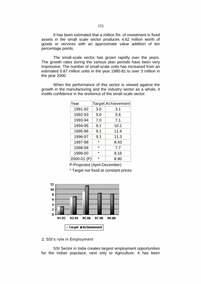
155

It has been estimated that a million Rs. of investment in fixedassets in the small scale sector produces 4.62 million worth ofgoods or services with an approximate value addition of tenpercentage points.

The small-scale sector has grown rapidly over the years.The growth rates during the various plan periods have been veryimpressive. The number of small-scale units has increased from anestimated 0.87 million units in the year 1980-81 to over 3 million inthe year 2000.

When the performance of this sector is viewed against thegrowth in the manufacturing and the industry sector as a whole, itinstills confidence in the resilience of the small-scale sector.

Year Target Achievement

1991-92 3.0 3.1

1992-93 5.0 5.6

1993-94 7.0 7.1

1994-95 9.1 10.1

1995-96 9.1 11.4

1996-97 9.1 11.3

1997-98 * 8.43

1998-99 * 7.7

1999-00 * 8.16

2000-01 (P) * 8.90

P-Projected (April-December)

* Target not fixed at constant prices

2. SSI’s role in Employment

SSI Sector in India creates largest employment opportunitiesfor the Indian populace, next only to Agriculture. It has been

156

estimated that 100,000 rupees of investment in fixed assets in thesmall-scale sector generates employment for four persons.

3. Generation of Employment - Industry Group-wise

Food products industry has ranked first in generatingemployment, providing employment to 0.48 million persons(13.1%). The next two industry groups were Non-metallic mineralproducts with employment of 0.45 million persons (12.2%) andMetal products with 0.37 million persons (10.2%).

In Chemicals & chemical products, Machinery parts exceptElectrical parts, Wood products, Basic Metal Industries, Paperproducts & printing, Hosiery & garments, Repair services andRubber & plastic products, the contribution ranged from 9% to 5%,the total contribution by these eight industry groups being 49%.In all other industries the contribution was less than 5%.

4. Per unit employmentPer unit employment was the highest (20) in units engaged

in beverages, tobacco & tobacco products mainly due to the highemployment potential of this industry particularly in Maharashtra,Andhra Pradesh, Rajasthan, Assam and Tamil Nadu.

Next came Cotton textile products (17), Non-metallic mineralproducts (14.1), Basic metal industries (13.6) and Electricalmachinery and parts (11.2.) The lowest figure of 2.4 was in Repairservices line.

Per unit employment was the highest (10) in metropolitanareas and lowest (5) in rural areas.

However, in Chemicals & chemical products, Non-metallicmineral products and Basic metal industries per unit employmentwas higher in rural areas as compared to metropolitan areas/urbanareas.

In urban areas highest employment per unit was inBeverages, tobacco products (31 persons) followed by Cottontextile products (18), Basic metal industries (13) and Non-metallicmineral products (12).

Location-wise Employment Distribution –

RuralNon-metallic products contributed 22.7% to employment

generated in rural areas. Food Products accounted for 21.1%,Wood Products and Chemicals and chemical products sharedbetween them 17.5%.

157

UrbanAs for urban areas, Food Products and Metal Products

almost equally shared 22.8% of employment. Machinery partsexcept electrical, Non-metallic mineral products, and Chemicals &chemical products between them accounted for 26.2% ofemployment.

In metropolitan areas the leading industries were Metalproducts, Machinery and parts except electrical and Paper products& printing (total share being 33.6%).

State-wise Employment Distribution

Tamil Nadu (14.5%) made the maximum contribution toemployment.

This was followed by Maharashtra (9.7%), Uttar Pradesh (9.5%)and West Bengal (8.5%) the total share being 27.7%.

Gujarat (7.6%), Andhra Pradesh (7.5%), Karnataka (6.7%) andPunjab (5.6%) together accounted for another 27.4%.

Per unit employment was high - 17, 16 and 14 respectively - inNagaland, Sikkim and Dadra & Nagar Haveli.

It was 12 in Maharashtra, Tripura and Delhi.

Madhya Pradesh had the lowest figure of 2. In all other cases it wasaround the average of 6.

Year Target(lakh nos.)

Achievement(lakh nos.)

Growth rate

1992-93 128.0 134.06 3.28

1993-94 133.0 139.38 3.28

1994-95 138.6 146.56 5.15

1995-96 144.4 152.61 4.13

1996-97 150.5 160.00 4.88

1997-98 165 167.20 4.50

1998-99 170.1 171.58 2.61

1999-00 175.4 177.3 3.33

P-Provisional

158

5. SSI’s role in Export:

SSI Sector plays a major role in India's present exportperformance. 45%-50% of the Indian Exports is contributed by SSISector. Direct exports from the SSI Sector account for nearly 35%of total exports. Besides direct exports, it is estimated that small-scale industrial units contribute around 15% to exports indirectly.This takes place through merchant exporters, trading houses andexport houses. They may also be in the form of export orders fromlarge units or the production of parts and components for use forfinished exportable goods.

It would surprise many to know that non-traditional productsaccount for more than 95% of the SSI exports.

The exports from SSI sector have been clocking excellentgrowth rates in this decade. It has been mostly fuelled by theperformance of garments, leather and gems and jewellery unitsfrom this sector.

The product groups where the SSI sector dominates inexports, are sports goods, readymade garments, woollen garmentsand knitwear, plastic products, processed food and leatherproducts.

The SSI sector is reorienting its export strategy towards thenew trade regime being ushered in by the WTO.

Year Exports (Rs. Crores)(at current prices)

1994-95 29,068 (14.86)

1995-96 36,470 (25.50)

1996-97 39,249 (7.61)

1997-98 43946 (11.97)

1998-99 48979 (10.2)

1999-00 (P) 53975 (10.2)

P-Provisional

159

These industries are also very important for welfare reasons.People of small means can organize these industries. This in turnincreases their income levels and quality of life. As such these canhelp in reducing poverty in the country. Further, these industriestend to promote equitable distribution of income. The reasons areobvious. One, a large proportion of income generated in theseenterprises is distributed among the workers. Two, income aredistributed among a vast number of persons throughout thecountry. All these benefits flow from the fact that these industriesare highly labour-intensive, and that these can be set up anywherein the country. Distributive aspect of small-scale industries furtherunravels their two-fold beneficial character. On the one hand, theseindustries enable a vast number of people to earn income, and onthe other hand, the very people among whom these are distributedgenerate this income

13.3 POLICY ISSUE AND PERFORMANCE

After independence, Indian planners and policy-makers feltthat protection was essential to the development of a strong andindigenous economy. The Indian state played an integral role in theindustrial and economic development of the country resulting in adominant public sector and heavily regulated private sector.Viewing this, the protection was also extended to SSI as it was animportant tool in employment generation, value creation andpoverty alleviation. These SSI also support entrepreneurial talentand skills, stimulate personal savings, and help in developinginnovative and appropriate indigenous technology, providingdynamism and contributing to competition. Over 800 products wereexclusively reserved for SSI, where some of the products producedwere purchased by government agencies. Apart form this, supply ofscarce materials, input price concessions like lower interest ratesand numerous fiscal measures such as excise duty exemptions andother tax concessions were also given (Source-Business Today,September 10, 2006).

Government has reserved certain products for manufacturein the small scale sector in areas where there is techno-economicjustification for such an approach. Large/Medium units can;however, manufacture such reserved items provided theyundertake to export 50% or more of their production. As on March2005, the total number of items reserved for small-scale sector is506.

In the second plan (1956-61), the SSI was given priority dueto its consequence in creation of diversified employmentopportunities and wide dispersal of industrial production. Thepolicies proposed then, were, and remain the main backbone ofpublic policy relating to the SSI. What we see however is that this

160

policy has been largely unhelpful, if not detrimental to thedevelopment of the sector. The policy regulations relating to theSSI are such that they ensure that units stay just small.

Promotional measures aim to increase the efficiency andeconomic viability of small units by providing infrastructure facilitiesand improving access to markets. On the other hand, protectivemeasures give small units preferential treatment. Continuousmeasures are those benefits which a small unit may avail of as longas it falls under that category, while one-shot are those which maybe availed of only once, and tends to be discretionary in nature.Most policies like preference in government purchases; lowerinterest rates etc. are continuous in nature. Discretionary measuresare those, which require an examination on a case-by-case basisand are not blanket measures available to all units, which fall underthe definition of small. Non discretionary, by implication, are thosemeasure which are based on some objective criteria and areapplicable to all units that meet the criteria. The government hasalso provided measures such as greater infra-structural support,more and easier availability of credit, lower rates of duty,technology up-gradation, assistance to build entrepreneurial talent,facilities for quality improvement, and export incentives.

The Ministry of Small Scale Industries (MoSSI) designspolicies, programmes, projects and schemes in consultation with itsorganizations. It also performs the function of policy advocacy withother Ministries/Departments of the Central Government and theStates and Union Territories. Implementation of the policies andprogrammes/projects/schemes for providing various supportservices to the MSEs is undertaken through its attached office,namely, the Office of Development Commissioner (Small ScaleIndustries) also known as Small Industries DevelopmentOrganisation (SIDO) and the National Small Industries Corporation(NSIC) Ltd., a public sector undertaking of the Ministry. There arethree national level Entrepreneurship Development Institutessupported by the Ministry viz. National Institute of Small IndustryExtension Training (NISIET), Hyderabad, National Institute ofEntrepreneurship and Small Business Development (NIESBUD),NOIDA and Indian Institute of Entrepreneurship (IIE),Guwahati.

Financial aid for SSI

Credit is the prime input for sustained growth of SSI and itsmobilization for meeting fixed and working capital needs poses theforemost problems. Credit provided for creation of fixed assets likeland, building, plant and machinery is called long term credit. Creditprovided for running the industry for its day-to-day requirement forpurchasing raw material and other input like electricity and wateretc. and for payment of wages and salaries is called short-termcredit or working capital.

161

The Laghu Udyami (small enterprise) Credit Card Schemehas been provided to SSI where they can credit up to Rs.10lakhs.Apart from this, credit facilities up to maximum of Rs.25lakhs areprovided through Credit Guarantee Fund Trust in collaboration withSIDBI and Govt. of India. Table X provides further insight into creditrelated information. The SSI is provided working capital bycommercial banks and in some cases by cooperative banks andregional rural banks. Term loans are provided by State FinancialCorporations (SFCs), Small Industries Development Corporations(SIDCs), National Small Industries Corporation (NSIC) and NationalBank for Agriculture and Rural Development (NABARD). Financialassistance from NSIC and to some extent from SIDCs is availablein the form of supply of machinery on hire purchase basis/deferredpayment basis. Small sized SSI and tiny units also get some termloans from commercial banks along with working capital in the formof composite loans. The Small Industries Development Bank ofIndia (SIDBI) provides refinance to these institutions. Suchrefinance comprises assistance provided to State FinancialCorporation Bills, Finance Scheme, Special Capital/Seed CapitalScheme, and new debt instruments and to National SmallIndustries Corporation. Long-term loan are provided to the smallsscale industrial units by SFCs mainly through Single WindowScheme and National Equity Fund as also direct assistanceprovided to State Financial Corporations in the form of refinance.Some part of working capital for pre-operative expenses is alsoprovided by State Financial Corporations to Small Scale IndustrialUnits under the Single Window Scheme.

13.4 SUMMARY:

Small industry sector has performed exceedingly well andenabled our country to achieve a wide measure of industrial growthand diversification. By its less capital intensive and high laborabsorption nature, SSI sector has made significant contributions toemployment generation and also to rural industrialization. Underthe changing economic scenario, SSI has both the challenges andopportunities before them. The business can compete on cost,quality and products at domestic and international level only if idealinvestment in technology production process, R&D and marketingare made. Infrastructure bottlenecks are not completely solved. Thepromotional activities for SSI in India need to concentrate onimproved credit flows, human resource development, appropriatetechnology and funds for modernization. It may be said that thestance is optimistic, indeed promising, given some protection. Thisexpectation is based on an essential feature of the Indian industryand the demand structures. The variety in the demand structureswill ensure long-term co-existence of many layers of demand forconsumer products / technologies / processes. There will beflourishing and well grounded markets for the same

162

product/process, differentiated by quality, value added andsophistication. This characteristic of the Indian economy will allowcomplementary existence for various diverse types of units.

13.5 QUESTIONS

1. Define small scale industry. Explain the role of SSI in IndianEconomic structure.

2. Explain policy issues & performance of SSI afterindependent.

163

14

INDUSTRIAL LOCATION ANDREGIONAL IMBALANCE

Unit Structure :

14.0 Objectives

14.1 Introduction

14.2 Weber’s theory of industrial location (The pure theory)

14.3 Regional imbalance : (Regional disparity and developmentpolicies in India)

14.4 Policy initiatives for balanced regional growth

14.5 Globalization

14.6 Privatization

14.7 Summary

14.8 Questions

14.0 OBJECTIVES

To study the meaning and factors influencing industriallocation.

To Study Weber’s Theory of industrial location. To study the causes of regional imbalance To study the impact of Globalization and Privation on Indian

industries.

14.1 INTRODUCTION

Location of industries is influenced by economicconsiderations though certain non-economic considerations alsomight influence the location of some industries. Maximisation ofprofit which also implies cost minimization is the most importantgoal in their choice of particular places for the location of industries.There are several factors which pull the industry to a particularplace. Some of the major factors influencing location are discussedbelow:

164

Factors Influencing Industrial Location

1. Availability of raw materials:In determining the location of an industry, nearness to sourcesof raw material is of vital importance. Nearness to the sources ofraw materials would reduce the cost of production of theindustry. For most of the major industries, the cost of rawmaterials form the bulk of the total cost. Therefore, most of theagro-based and forest-based industries are located in thevicinity of the sources of raw material supply.

2. Availability of Labour:Adequate supply of cheap and skilled labour is necessary forand industry. The attraction of an industry towards labourcentres depends on the ratio of labour cost to the total cost ofproduction which Weber calls ‘Labour cost of Index’. Theavailability of skilled workers in the interior parts of Bombayregion was one of the factors responsible for the initialconcentration of cotton textile industry in the region.

3. Proximity to Markets:Access to markets is an important factor which theentrepreneur must take into consideration. Industries producingperishable or bulky commodities which cannot be transportedover long distance are generally located in close proximity tomarkets. Industries located near the markets could be able toreduce the costs of transport in distributing the finished productas in the case of bread and bakery, ice, tins, cansmanufacturing, etc. Accessibility of markets is more important inthe case of industries manufacturing consumer goods ratherthan producer goods.

4. Transport Facilities:Transport facilities, generally, influence the location of industry.The transportation with its three modes, i.e., water, road, andrail collectively plays an important role. So the junction points ofwater-ways, roadways and railways become humming centresof industrial activity. Further, the modes and rates of transportand transport policy of Government considerably affect thelocation of industrial units. The heavy concentration of cottontextile industry in Bombay has been due to the cheap andexcellent transportation network both in regard to raw materialsand markets.

5. Power:Another factor influencing the location of an industry is theavailability of cheap power. Water, wind, coal, gas, oil andelectricity are the chief sources of power. Both water and windpower were widely sought at sources of power supply before the

165

invention of steam engine. During the nineteenth century,nearness to coal-fields became the principal locating influenceon the setting up of new industries, particularly, for heavyindustries. With the introduction of other sources of power likeelectricity, gas, oil, etc. the power factor became more flexibleleading to dispersal and decentralization of industries.

6. Site and Services:Existence of public utility services, cheapness of the value of thesite, amenities attached to a particular site like level of ground,the nature of vegetation and location of allied activities influencethe location of an industry to a certain extent. The governmenthas classified some areas as backward areas where theentrepreneurs would be granted various incentives likesubsidies, or provision of finance at concessional rate, or supplyof power a cheaper rates and provision of education andtraining facilities. Some entrepreneurs induced by suchincentives may come forward to locate their units in such areas.

7. Finance:Finance is required for the setting up of an industry, for itsrunning, and also at the time of its expansion. The availability ofcapital at cheap rates of interests and in adequate amount is adominating factor influencing industrial location. For instance, areview of locational history of Indian cotton textile industryindicates that concentration of the industry in and aroundBombay in the early days was mainly due to the presence ofrich and enterprising Parsi and Bhatia merchants, who suppliedvast financial resources.

8. Natural and Climatic Considerations:Natural and climatic considerations include the level of ground,topography of a region, water facilities, drainage facilities,disposal of waste products, etc. These factors sometimesinfluence the location of industries. For instance, in the case ofcotton textile industry, humid climate provides an addedadvantage since the frequency of yarn breakage is low. Thehumid climate of Bombay in India and Manchester in Britainoffered great scope for the development of cotton textileindustry in those centres.

9. Personal Factors:In deciding location of industrial units, sometimes anentrepreneur may have personal preferences and prejudicesagainst certain localities. For instance, Mr. Ford started tomanufacture motor cars in Detroit simply because it was hishome-town. In such cases, personal factor dominates otherconsiderations. However, this kind of domination is rare.

166

10.Strategic Considerations:In modern times, strategic considerations are playing a vital rolein determining industrial location. During war-time a safelocation is assuming special significance. This is because intimes of war the main targets of air attacks would be armamentand ammunition factories and industries supplying othercommodities which are required for war. The Russianexperience during the Second World War provides andinteresting example.

11.External Economies:External economies also exert considerable influence on thelocation of industries. External economies arise due to thegrowth of specialized subsidiary activities when a particularindustry is mainly localized at a particular centre with port andshipping facilities. External economies could also be enjoyedwhen a large number of industrial units in the same industrywere located in close proximity to one another.

12.Miscellaneous Factors:Historical incidents also play a dominating role in determiningthe location of industries in certain cases. The development ofcotton-textile industry in Lancashire provides an interestingexample for this. Further, the size of and industrial unit wouldalso have much influence in choosing location. This is becausethe size of industrial units depends upon the radius of the circlewithin which they can profitably distribute their goods and uponthe density of population living within the circle.

14.2 WEBER’S THEORY OF INDUSTRIAL LOCATION(THE PURE THEORY)

Alfred Weber, a German economist, enunciated a systematictheory of industrial location in 1909. Weber’s theory of location ispurely deductive in its approach. He analyzed the factors thatdetermine the location of industry and classified these factors intotwo divisions. These are:

(i) Primary causes of regional distribution of industry (regionalfactors)

(ii) Secondary causes (agglomerative and deglomerative factors)that are responsible for redistribution of industry.

(i) Primary Causes (Regional Factors)According to Weber, transport costs and labour costs are the

two regional factors on which his pure theory is based. Assumingthat there are no other factors that influence the distribution ofindustry, except transportation costs. Then it is clear that the

167

location of industry will be pulled to those locations which have thelowest transportation costs. The key factors that determinetransportation costs are

(i) the weight to be transported and(ii) the distance to be covered.

Weber lists some more factors which influence thetransportation costs such as – (a) the type of transportation systemand the extent of its use, (b) the nature of the region and kinds ofroads, (c) the nature of goods themselves, i.e., the qualities which,besides weight, determine the facility of transportation.

However, the location of the place of production must bedetermined in relation to the place of consumption and to the mostadvantageously located material deposits. Thus, ‘locational figures’are created. These locational figures depends upon (a) the type ofmaterial deposits and (b) the nature of transformation into products.Weber classifies and calls those raw materials, which are availablepractically everywhere as ‘ubiquities’ (like brick-clay, water, etc) and‘localised’ (like iron-ore, minerals, wood, etc) which are availableonly in certain regions. It is clear that localized materials play amore important role on the industry than the ubiquities. Further,regarding the nature of the transformation of materials intoproducts, Weber categorized the raw materials as ‘pure’ and‘weight losing’. Pure materials impart their total weight to theproducts (eg. cotton, wool, etc) and the materials are said to be‘weight losing’ if only a part enters into the product (eg. wood, coal,etc.). Hence, the location of industries using weight-losing materialsis drawn towards their deposits and that of industries using pure-materials towards the consumption centres.

Weber further examines the cause of deviation of industriallocation from the centres of least transport costs. The existence ofdifferences in labour costs leads an industry to deviate from theoptimal point of transport orientation. Geographical distribution ofthe population would give rise to differences in wages for labour.Naturally, the transport oriented location of an industry is drawn outand attracted towards the cheaper labour centres. Such migrationof an industry from a point of minimum transport costs to a cheaperlabour centre may be likely to occur only where the savings in thecost of labour are larger than the additional costs of transport whichit ought to incur.

(ii) Secondary Causes (Agglomerative and DeglomerativeFactors)

An agglomerative factor is an advantage or a cheapening ofproduction or marketing which results from the fact that productionis carried on at one place. A deglomerative factor is a cheapening

168

of production which results from the decentralization of productioni.e., production in more than one place. To some extent theseagglomerative and deglomerative factors also contribute to localaccumulation and distribution of industry. These factors will operateonly within the general framework formed by the two regionalfactors, i.e., costs of transportation and costs of labour. Theadvantages which could be derived in this context are externaleconomies.

The pulls which the agglomerative factors possess to attractan industry to a particular point are mainly dependent on twofactors. Firstly, on ‘the index of manufacture’ (the proportion ofmanufacturing costs to the total weight of the product) andsecondly, on the ‘locational weight’ (the total weight to betransported during all the stages of production). To deduce ageneral principle, Weber uses the concept of “co-efficient ofmanufacture” which is the ratio of manufacturing cost to locationalweight. Agglomeration is encouraged with high co-efficient ofmanufacture and deglomeration with low co-efficient ofmanufacture and these tendencies are inherent in their nature.

Split Location:Productive activities could be divided depending on the

nature of raw-materials, industry and market. Weber considers thelocation for an industry at more than one place. According toWeber, a split of production into several locations will be the rule forproductive process which can technically be split. For instance, thefirst stage of production may be near the raw material deposits andthe subsequent stages near the place of final consumption.Likewise, in a paper industry the manufacture of pulp may becarried on near the supplies of the raw materials and the secondstage of paper manufacture near the consumption outlet.

Locational Coupling:Weber also conceived the advantages of setting up different

types of industries in the same locality. The production of quitedifferent articles may be combined in one plant because severalraw materials may diverge from a common source. This may beeither due to technical or economic reasons: for instance, certainchemical industries, garments factories which manufacture over-coats, shawls, blouses, etc. Locational coupling may also occur dueto connection through materials. If the by-product of an industryhappens to be the raw material of another industry, then the twoindustries may select a single place of location. For instance, thedye-stuff industry is connected with other industries using coke,because coal tar (upon which the dye-stuff industry is based) is aby-product of the burning coke.

169

Criticisms:Weber’s theory of location has been criticized on various

grounds which may be summarized as follows:

1. Weber has been criticized for his unrealistic approach anddeductive reasoning. According to Sargant Florence, vaguegeneralizations cannot provide suitable solutions to the theory oflocation as non-economic considerations will also influence whichare not mentioned in the pure theory. He says that Weber’s theoryfails to explain locations resulting from historical and social forces.2. A.Predohl criticizes Weber’s theory as more a selective theorythan a deductive theory. The very distinction between primary andsecondary is itself artificial, illogical and arbitrary.

3. Weber assumes fixed labour centres and unlimited supplies oflabour which are unrealistic. The rise of industry may create newlabour centres and we cannot assume unlimited labour supplies atany centre.

4. In a competitive market structure, the assumption of fixed pointsof consumption is unrealistic. Country-wise scattering, usually, ofconsuming public is a reality and there may be a shift in theconsuming centres with a shift in industrial population.

5. A. Robinson also considers Weber’s division of raw materialsinto ‘ubiquities’ and ‘localised’ as artificial.

Weber’s deductive theory of location, in spite of theshortcomings, is the only theory which has been neither enjoyingthe universal acceptance and application, as all the otheralternative suggestions are neither complete nor comprehensive.

14.3 REGIONAL IMBALANCE: (Regional disparity anddevelopment policies in India)

I) Post-Independence Period:

Government’s economic policies during the colonial periodwere more to protect the interests of the British economy ratherthan for advancing the welfare of the Indians. The primaryconcerns of the Government were law and order, tax collection anddefence. As for development, Government adopted a basicallylaissez-faire attitude. Of course, railways, irrigation systems, roadnetwork and modern education system were developed during thisperiod. Railways and road network were more to facilitatemovements of goods and defence personnel and to facilitate betteradministrative control. Irrigation canal system was mainly to fightrepeated droughts and famines and to boost land revenue.

170

Education, to begin with, was developed mainly to train lower-ranking functionaries for the colonial administration.

Particularly lacking was a sustained positive policy topromote indigenous industry. Indeed, it is widely believed thatgovernment policies, far from encouraging development, wereresponsible for the decline and disappearance of much of India’straditional industry.

Altogether, the pre-independence period was a period ofnear stagnation for the Indian economy. The growth of aggregatereal output during the first half of the twentieth century is estimatedat less than two per cent per year, and per capita output by half of aper cent a year or less.

There was hardly any change in the structure of productionor in productivity levels. The growth of modern manufacturing wasprobably neutralised by the displacement of traditional crafts, and inany case, was too small to make a difference to the overall picture.

Along with an impoverished economy, independent Indiaalso inherited some useful assets in the form of a national transportsystem, an administrative apparatus in working order, a shelf ofconcrete development projects and a comfortable level of foreignexchange. While it is arguable whether the administrativeapparatus built by the British helped or hindered development since1947, there is little doubt that its existence was a great help incoping with the massive problems in the wake of independencesuch as restoring civil order, organising relief and rehabilitation formillions of refugees and integrating the Princely States to theUnion.

The development projects initiated in 1944 as a part of thePost-war Reconstruction Programme was of particular value toIndependent India’s first government. Under the guidance of thePlanning and Development Department created by the CentralGovernment, a great deal of useful work was done beforeIndependence to outline the broad strategy and policies fordeveloping major sectors and to translate them into programmesand projects. By the time of Independence several of these werealready under way or ready to be taken up. They includedprogrammes and projects in agriculture, irrigation, fertilizer,railways, newsprint and so on. Though the first Five Year Planbegan in 1950-51, with the establishment of Planning Commission,a well-rounded planning framework was in place only with thesecond Five Year Plan after five years. By and large, the basis ofthe first Five Year Plan was the groundwork done beforeindependence. Most of the principal projects were continuationsand major efforts were made to complete them early.

171

II. Recent Trends

Regional disparities are the result of our unfinished task ofnation building. These reflect essentially the inadequacies of thedevelopment strategy followed since independence and its failureto correct the distortions brought about by colonial rule. Of late,these tensions have acquired alarming proportions and arethreatening to strike at the very roots of the nation state. This hasbrought to sharp focus the need of better understanding of thepattern of regionalization, the nature of regional imbalances andtheir changing structure over time.

Hence, balanced regional development is necessary for theharmonious growth of federal state like India, however, presents apicture of wide regional variations, in terms of per capita income,proportion of population living below the poverty line, workingpopulation in agriculture, the percentage of urban population overtotal population, etc.

To study the regional imbalance, the 15 major states of Indiahave been classified into two major groups

Imbalance in per capita :

172

Since, per capita income shows the average annualearnings of a single person in a particular region. It can be treatedas an indicator for regional development. As the past record showsthat the Punjab topped the list as it had the highest per capitaincome in 1990-91 and Orissa was at bottom. In 2002-03,Maharashtra was at top and Bihar was at bottom on the basis ofper capita income. However, this list was again changed in 2005-06, Haryana was at top and Bihar was at bottom on the basis of percapita income. This implies that the backward states with very largepopulation share – U.P., Bihar and Madhya Pradesh – acted as adrag on the growth process of the Indian Economy.

Indian economy has experienced an average annual growthrate of around 6 per cent during the last two decades. Though,moderate compared to the performance of several east Asianeconomies during the same period, this was quite impressivecompared to the performance of Indian economy during thepreceding three decades when the average growth logged 3.5 percent per annum. Even the growth rate of 3.5 per cent experiencedduring the first three decades of the republic had beenspectacularly better that the virtual stagnation of the Indianeconomy during the first half of the Twentieth Century. In terms ofper capita income, the improvement has been even moreremarkable - around 4 per cent per annum in the recent period ascompared to less than 1.5 per cent in the earlier period. Further,during the recent period, there has been a steady acceleration inthe growth performance over the years. The average compoundgrowth per annum was 5.7 per cent during the Sixth Five Year Plan(1980-85), 6.0 per cent during the Seventh Plan (1985-90) and 6.6per cent during the Eighth Plan (1992-97). While the growth ratedropped to 3.1 per cent during the two-year period 1990-92 in thewake of international payment crisis and the introduction of majoreconomic reforms, the growth process picked up fast in thesubsequent years. Indeed, the growth averaged about 7.5 per centduring the three-year period ending 1996-97, which is impressiveby any standards. The growth rate has been somewhat lower inthe subsequent three years. In contrast to stagnation/negativegrowth of most of the East Asian economies India’s performance,however, is remarkable. The World Bank and other internationalagencies have characterized India as one of the fastest growingeconomies of the world.

As is to be expected, improvement in economic growth andper capita income translated, at least partly, into reduction in thelevel of poverty in the country. Though there are differences in theestimates of the percentage of the poor by different sources, allagree that there has been a secular decline in the share of poor inthe population since the late Seventies. The official estimates ofpopulation below poverty line released by the Planning Commission

173

on the basis of the Expert Group methodology indicate this seculardownward trend:

Year 1977-78 1983 1987-88 1993-94 1999-2000

Percentageof poor

51.3 44.5 38.9 36.0 26.10

The last two decades had seen the introduction/expansion ofseveral anti-poverty programmes and public intervention policies infavour of the poor including public distribution of subsidized foodgrains. The reduction in poverty in the recent period is attributed toanti-poverty programmes by their protagonists and to acceleratedeconomic growth by market friendly experts.

Along with faster economic growth and reduction in poverty,there has been accelerated improvement in various indicators ofhuman development since the early Eighties whether it is in thecase of demographic characteristics or social developmentindicators. During the last two decades, the country has mademajor strides in health and education sectors. The economy gotdiversified significantly and the share of the service sector inemployment and incomes improved considerably. While there is abroad consensus on the overall improvement of the economy andquality of life during the period under consideration, there aresignificantly differing perceptions about the distributional impacts ofthese gains.

Disparities in economic and social development across theregions and intra-regional disparities among different segments ofthe society have been the major planks for adopting planningprocess in India since independence. Apart from massiveinvestments in backward regions, various public policies directed atencouraging private investments in such regions have beenpursued during the first three decades of planned development.While efforts to reduce regional disparities were not lacking,achievements were not often commensurate with these efforts.Considerable level of regional disparities remained at the end of theSeventies. The accelerated economic growth since the earlyEighties appears to have aggravated regional disparities. The on-going economic reforms since 1991 with stabilisation andderegulation policies as their central pieces seem to have furtherwidened the regional disparities. The seriousness of the emergingacute regional imbalances has not yet received the public attentionit deserves.

Most of the studies on inter-country and inter-regionaldifferences in levels of living and income are done within thetheoretical framework of neoclassical growth models. These

174

models, under plausible assumptions demonstrate convergence ofincomes. Three notable recent studies3, however, indicate that inthe Indian context these convergence theories do not explain theground realities.

The scope of analysis in this section is restricted to acomparative analysis of the emerging trends in fifteen major States4

in respect of a few key parameters which have an intrinsic bearingon social and economic development. The variables chosen forexamination include those which have a bearing on gender andequity issues. The fifteen States together account for 95.5 per centof the population of India. The remaining 4.5 per cent of thepopulation is spread out in 10 smaller States and seven UnionTerritories including the National Capital Territory of Delhi. Leavingout these States and UTs from detailed study is mainly due to non-availability of all relevant data and also to keep the data setsanalytically and logistically manageable. The fifteen States taken upfor the detailed study have been grouped into two - a forward groupand a backward group. The forward group consists of AndhraPradesh, Gujarat, Haryana, Karnataka, Kerala, Maharashtra,Punjab and Tamil Nadu. The backward group comprises of Assam,Bihar, Madhya Pradesh, Orissa, Rajasthan, Uttar Pradesh andWest Bengal.

Geographically, the forward group of States fall in theWestern and Southern parts of the country and are contiguousexcept for Punjab and Haryana which are separated by Rajasthanfrom the rest of the States in this group. The group of backwardStates are in the Eastern and Northern parts of the country and aregeographically contiguous. Another notable geographical feature isthat while six out of eight States, except Haryana and Punjab, in thefirst group have vast sea coasts, only two out of the seven in thesecond group viz., Orissa and West Bengal are littoral. While theforward group of States account for about 40.4 per cent of thenational population, the backward group accounts for as much as55.1 per cent of the population of the country according to 2001census5. In terms of natural resources including mineral wealth,water resources and quality of soil, the latter has definite edge overthe former.

A limitation of inter-regional analysis using States as units isthe fact that this may not be able to capture the significant intra-State disparities in economic and social development, which existstoday. The larger States in both the groups have regions withinthemselves, which are vastly different in terms of various indicatorsof development. There are identifiable distinct regions, at differentstages of development, in several States. After discussing theinter-regional disparities in development, treating States as units,we will take up intra-State disparities for a brief analysis in the latterpart of the present study.

175

14.4 POLICY INITIATIVES FOR BALANCEDREGIONAL GROWTH

We shall initiate the discussion on initiatives for balancedregional growth by illustrating two instances of initiatives in the past.One relates to agriculture and the other relates to industry, the twomost important sectors of our economy. The strategy to boostagricultural production and to ensure food security was evolved inthe mid-Sixties when the country faced a grim situation followingtwo consequent years of severe draught. The strategy consisted ofvarious incentives to farmers to adopt high yielding seeds of wheatand paddy along with complimentary inputs, assured minimumsupport prices for the output, buffer stocking of the foodgrains andsupplying the same to the States to distribute through the publicdistribution system (PDS) to the consumers, especially in the deficitregions. To back up this strategy, institutions like AgriculturalPrices Commission (APC), Food Corporation of India (FCI) andWarehousing Corporation of India and other ancillary institutionswere established. Arrangements were made to spread themessage of high yielding seeds and the associated package ofinputs and practices.

The above strategy ushered in a green revolution, whichresulted in doubling of wheat and rice production in the countryover a short period. Adequate foodgrains surpluses weregenerated to build up the needed buffer stock. India was no more a‘basket case’.

The initial success of green revolution strategy wasrestricted to Punjab, Haryana and western Uttar Pradesh whereassured irrigation networks already existed. Subsequently it wasextended to a few irrigation commands in the South and West also.It was, however, expected that with the expansion of assuredirrigation the green revolution would spread to other parts of thecountry soon. In the event this did not happen. Even today almostthe entire foodgrain surpluses are generated by the small region,which benefited initially. Though massive public funds are spent onfood subsidies, very little is spent on spreading irrigation. Besidesfood subsidies, large implicit subsidies to farmers for power, diesel,canal irrigation, fertilizer and credit are born by public exchequer atthe Centre and in the States.

Agricultural Price Policy which was evolved by APC toensure adequate protection to the interests of the producers andconsumers has been ‘high-jacked’ to serve the interests of the largefarmers who produce for the market. It hardly serves the interestsof farmers in the emerging surplus regions. The distinctionbetween support price and procurement price is no more there.

176

Similarly, the Food Corporation of India and the associatedprocurement agencies operate, by and large, only in the traditionalsurplus regions and farmers in newly emerging surplus regionsalmost invariably end up selling their surpluses in distress.

Today the foodgrain management and the food securitysystem is near collapse. As against a total requirement of 24million tonnes of foodgrain for buffer stock and PDS together, thepublic stock is over 60 million tones as on July 1,2001. Asubstantial share of this is not even properly stored and may not besuitable for human consumption. On the other hand due to severedrought conditions large scale unemployment and hunger arereported from several States. Per capita net availability in themarket has come down. PDS system has virtually collapsed. Poorpeople cannot afford the ‘so called economic price’ of foodgrainsavailable in the PDS shops.

The economic liberalization policy initiated since the early1991 has made large-scale delicensing of industry and changes inthe industrial location policies, and thus, curtailed the role of thestate as industrial owner and location regulator. With the increasingdominance of private sector in industrialization under liberalization itis expected that industries will be more spatially concentrated in theleading industrial regions. However, the neoclassical principlesuggests that in the long run "divergence is followed byconvergence". This is in contrast with the theory that raises thequestion about the regional industrial development in India underthe two policy regimes.

Industrial undertakings are free to select the location of aproject. In the case of cities with population of more than a million(as per the 1991 census), however, the proposed location shouldbe at least 25 KM away from the Standard Urban Area limits of thatcity unless, it is to be located in an area designated as an‘’industrial area’’ before the 25th July, 1991. (List of cities withpopulation of 1 million and above is given at Annexure-V).Electronics, Computer software and Printing (and any otherindustry which may be notified in future as “non polluting industry”)are exempt from such location restriction. Relaxation in theaforesaid location restriction is possible if an industrial license isobtained as per the notified procedure.

The location of industrial units is further regulated by thelocal zoning and land use regulations as also the environmentalregulations. Hence, even if the requirement of the location policystated in paragraph 1.3 is fulfilled, if the local zoning and land useregulations of a State Government, or the regulations of theMinistry of Environment do not permit setting up of an industry at alocation, the entrepreneur would be required to abide by thatdecision.

177

Liberalisation of the Location Policy A significantly amendedlocational policy in tune with the liberlised licensing policy is inplace. No industrial approval is required from the Government forlocations not falling within 25 kms of the periphery of cities having apopulation of more than one million except for those industrieswhere industrial licensing is compulsory. Non-polluting industriessuch as electronics, computer software and printing can be locatedwithin 25 kms of the periphery of cities with more than one millionpopulation. Permission to other industries is granted in suchlocations only if they are located in an industrial area so designatedprior to 25.7.91. Zoning and land use regulations as well asenvironmental legislations have to be followed.

Policy for Small Scale A differential investment limit has beenadopted since 9th October 2001 for 41 reserved items where theinvestment limit upto rupees five crore is prescribed for qualifyingas a small scale unit. The investment limit for tiny units is Rs. 25lakhs.

749 items are reserved for manufacture in the small scale sector.All undertakings other than the small scale industrial undertakingsengaged in the manufacture of items reserved for manufacture inthe small scale sector are required to obtain an industrial licenceand undertake an export obligation of 50% of the annualproduction. This condition of licensing is, however, not applicable tothose undertakings operating under 100% Export OrientedUndertakings Scheme, the Export Processing Zone (EPZ) or theSpecial Economic Zone Schemes (SEZs).

Non-Resident Indians SchemeThe general policy and facilities for Foreign Direct

Investment as available to foreign investors/company are fullyapplicable to NRIs as well. In addition, Government has extendedsome concessions specially for NRIs and overseas corporatebodies having more than 60% stake by the NRIs. These inter-aliaincludes (i) NRI/OCB investment in the real estate and housingsectors upto 100% and (ii) NRI/OCB investment in domestic airlinessector upto 100%.NRI/OCBs are also allowed to invest upto 100%equity on non-repatriation basis in all activities except for a smallnegative list. Apart from this, NRI/OCBs are also allowed to investon repatriation/non-repatriation under the portfolio investmentscheme.

Electronic Hardware Technology Park (EHTP)/SoftwareTechnology Park (STP) scheme for building up strong electronicsindustry and with a view to enhancing export, two schemes viz.Electronic Hardware Technology Park (EHTP) and SoftwareTechnology Park (STP) are in operation. Under EHTP/STPscheme, the inputs are allowed to be procured free of duties.

178

The Directors of STPs have powers to approved fresh STP/EHTPproposals and also grand post-approval amendment in repsect ofEHTP/STP projects as have been given to the DevelopmentCommissioners of Export Processing Zones in the case of ExportOriented Units. All other application for setting up projects underthese schemes, are considered by the Inter-Ministerial StandingCommittee (IMSC) Chaired by Secretary (Information Technology).The IMSC is serviced by the SIA.

Policy for Foreign Direct Investment (FDI)The Department hasput in place a liberal and transparent foreign investment regimewhere most activities are opened to foreign investment onautomatic route without any limit on the extent of foreign ownership.Some of the recent initiatives taken to further liberalise the FDIregime, inter alia, include opening up of sectors such as Insurance(upto 26%); development of integrated townships (upto 100%);defence industry (upto 26%); tea plantation (utp 100% subject todivestment of 26% within five years to FDI); Encenhancement ofFDI limits in private sector banking, allowing FDI up to 100% underthe automatic route for most manufacturing activities in SEZs;opening up B2B e-commerce; Internet Service Providers (ISPs)without Gateways; electronic mail and voice mail to 100% foreigninvestment subject to 26% divestment condition; etc.

14.5 GLOBALIZATION

One of the most significant changes in the world economyover the past two decades has been a growing globalization ofmarkets and industries. Numerous forces have contributed to risingglobalization, including reductions in multilateral and regional tradebarriers, reduced costs of international transport andcommunications and reform and greater global integration of capitalmarkets. The ongoing consequences of globalization includewidespread industry rationalization and heightened competition atnational, regional, and global levels as evidenced by significantlyhigher levels of foreign competition and increases in both cross-border mergers and acquisitions and the number of multinationalfirms.1 Increasing vertical linkages, as production activities becomemore specialized and spatially dispersed,2 have complemented thegrowing horizontal linkages among nations. The ongoing processesof globalization, particularly changes in the competitive conditionsfacing firms as markets and industries globalize, are significanteconomic phenomena that can, like other phenomena that changea firm’s business and competitive conditions, be expected to inducechanges in corporate strategy. Such influences may in particularimpact a firm’s international diversification strategy, defined as thedecision to expand

179

Definition: Though the precise definition of globalisation is stillunavailable a few definitions worth viewing, Stephen Gill: definesglobalisation as the reduction of transaction cost of transbordermovements of capital and goods thus of factors of production andgoods. Guy Brainbant: says that the process of globalisation notonly includes opening up of world trade, development of advancedmeans of communication, internationalisation of financial markets,growing importance of MNC's, population migrations and moregenerally increased mobility of persons, goods, capital, data andideas but also infections, diseases and pollution

Globalization and competition:

1) The causes of increased global trade include:

• Economic growth itself which both creates ever increasingdemand for imports and also increases the capacity ofeconomies to produce exports; it also generates greateramounts of savings which may be invested domestically andinternationally to meet the greater investment demandsassociated with economic growth.

• Technological innovation. This pervades most fields ofeconomic activity but is especially great in the areas ofinformation and communication technology. A sectorparticularly affected by technological growth in these areas isthe financial services sector which, in turn, facilitates higherdegrees of financial and economic interaction betweeneconomies in different countries.

• Falling transport costs.

• International, as well as domestic, liberalisation of trade,investment and economic activity generally.

It is important to note that the European Union has beenparticularly active in trying to promote a global approach tocompetition policy and in promoting the inclusion of competitionissues in the next round of trade negotiations at the WTO.

2) Global CartelsGlobal cartels, that is, cartels organised on an international

scale, have been in existence since the beginnings of internationaltrade. There is a long history of cartels, in particular, during thenineteenth and early parts of the twentieth century. Indeed, in 1907an important US Antitrust case sought to end the tobacco cartelwhich had divided up world markets between British producers,who controlled the UK; US producers, who controlled the US; andthe rest of the world, which was divided up and allocated to either

180

British or American producers who agreed not to compete in oneanother's markets.

3) Global mergers:In recent times there has been a spectacular increase in the

extent of international merger activity, in one sector after another

finance, communications, oil, airlines, pharmaceuticals, automotiveprofessional services and so on. For the most part, these mergersare not anticompetitive and pose no major challenge to the globaleconomy's major competitiveness. Indeed, in many cases, theyenhance competitiveness and improve economic efficiency bycreating more efficient arrangements for international businesstransactions.

4) Globalizations facilitated by rapid advances in technology,are creating new dynamics of competition and, in so doing, renderthe determinants of competitiveness much more complex. Asalready established in the preceding discussion, greater efficiencyis the source of competitiveness. In the context of internationaltrade, competitiveness is traditionally defined in terms of exchangerates, costs and prices. Nowadays a distinction is drawn betweenstatic competitiveness and dynamic competitiveness.2 In theformer, the emphasis is on price competition whereby firmscompete on the basis of received endowments such as low-costlabour and natural resources. Under these circumstances, retainingcompetitiveness is dependent on maintaining or loweringproduction costs. This is the basis on which many developingcountry firms compete. Dynamic competitiveness is associated withthe changing nature of competition, which places a premium notonly on the relationship between costs and prices but also on firm-level ability to learn, rapidly adjust to new market conditions andinnovate (where innovation is defined in the broadest terms and isnot necessarily confined to radical technological innovation).3 Inthis framework, competitiveness refers to the ability of firms toproduce goods and services that stand the test of internationalcompetition, while upgrading technological capabilities.

5) With globalization and liberalization, the boundaries betweennational and international markets have become blurred, traditionaldistinctions between national and international competitivenessthus becoming redundant. This blurring of boundaries hasimplications particularly for small and medium-sized enterprises(SMEs), which were previously insulated from internationalcompetition by national borders. A lack of finance and insufficienttechnological capabilities limit the ability of even firms that weredomestically competitive prior to liberalization to respond tocompetition that cuts too quickly into their market share. Inunderdeveloped markets with few participants, technologicallearning can be extremely risky and expensive for the individual

181

firm and is often not undertaken in the absence of supportingpolicies to facilitate their adjustment.

6) A notable feature of the changing nature of competition is aradical alteration in the organization of firms as well as theorganization of production, marketing and distribution of goods andservices at the international and national levels. In order to adaptand remain competitive firms are exploiting externalities or“knowledge spillovers” through inter-firm cooperation. Access toand possession of knowledge, in addition to technical hardware,has become an important asset for global producers. Networkingand being part of a production network is an increasingly importantway in which firms get to “know-what”, “know-how”, “know-why” andknow-who” in their particular line of business. The importance ofinnovation, and its research and development costs, has given riseto the duality of cooperation and competition.

7) An increasingly significant form of inter-firm cooperation andcoping mechanism utilized by firms in the face of the newcompetition is mergers and acquisitions. Globalization, capitalmarket pressures, the evolution of technical infrastructure requiredto support networking and the advent of the Internet haveprecipitated global industry consolidation. Among the industries inwhich this trend towards consolidation is documented are bankingand financial services, cigarettes, petroleum products, airlines,telecommunications, chemicals, sport shoes, beverages,automobile production and food services. According to a recentstudy on the phenomenon,5 at the end of the various stages ofconsolidation, the three largest market participants will typicallyhave captured 70–80 per cent of the market.

8) Although high concentration does not necessarily equatewith a lack of competition and need not have a negative impact oneconomic performance, it does facilitate the exercise of marketpower and anti-competitive behaviour.6 The duality betweencooperation and competition is not only a justification for countriesto develop and enforce competition policies, but it also demandsincreased vigilance and sophistication on the part of competitionpolicy enforcement authorities to ensure that cooperation does notlend itself to anticompetitive behaviour by merged or networkedfirms, care being taken at the same time not to stifle innovation and,in so doing, competition and competitiveness.

14.6 PRIVATIZATION

The term "privatization" also has been used to describe twounrelated transactions. The first is a buyout, by the majority owner,of all shares of a public corporation or holding company's stock,

182

privatizing a publicly traded stock, and often described as privateequity. The second is a demutualization of a mutual organization orcooperative to form a joint stock company.

Privatization is frequently associated with industrial orservice-oriented enterprises, such as mining, manufacturing orpower generation, but it can also apply to any asset, such as land,roads, or even rights to water. In recent years, government servicessuch as health, sanitation, and education have been particularlytargeted for privatization in many countries.

Privatization is the incidence or process of transferring ownershipof a business, enterprise, agency or public service from the publicsector (the state or government) to the private sector (businessesthat operate for a private profit) or to private non-profitorganizations. In a broader sense, privatization refers to transfer ofany government function to the private sector - includinggovernmental functions like revenue collection and lawenforcement.

In theory, privatization helps establish a "free market", aswell as fostering capitalist competition, which its supporters arguewill give the public greater choice at a competitive price.Conversely, socialists view privatization negatively, arguing thatentrusting private businesses with control of essential servicesreduces the public's control over them and leads to excessive costcutting in order to achieve profit and a resulting poor quality service.

In general, nationalization was common during the immediate post-World War 2 period, but privatization became a more dominanteconomic trend (especially within the United States and the UnitedKingdom) during the 1980s and '90s. This trend of privatization hasoften been characterized as part of a "global wave" of neoliberalpolicies, and some observers argue that this was greatly influencedby the policies of Reagan and Thatcher. The term "privatization"was coined in 1948 and is thought to have been popularized by TheEconomist during the '80s.

Indian scenario:1) The process of privatization in India is linked with the economic

reforms launched in 1991. The trigger for the reforms was asevere financial crisis the government faced. Caused by theprofligate external borrowing of the eighties and the 1991 Gulfcrisis, a severe shortage of foreign exchange led to a situationwhere basic petroleum supplies could not be obtained. Underpressure from the World Bank and the International MonetaryFund (IMF), the government agreed to several macroeconomicreforms. At that time it was realized that a process of

183

microeconomic reforms could be implemented. Several of theseended the policy of trade and industrial licensing that the‘licence raj’ had been built on. These opened up the Indianindustry to the forces of entrepreneurship and competition, andmade Indian markets contestable. The entry by privateenterprises into sectors that were reserved for the state orwhere the state had a significant presence could, therefore,create competitive pressures on existing state-owned units toperform better, or through a process of atrophy reduce theproportion of overall low performing units in Indian industry as awhole.

2) With respect to the issue of privatization, the governmentrecognized the need, from a fiscal perspective, of superiorperformance from the public sector. State-owned enterpriseswere an economic deadweight, causing substantial losses to theeconomy. The main activities during the reforms process werethat of de-licensing and removal of controls. These activitiesrequired notification processes to be undertaken, and these tobe undertaken by the ministries concerned, rather than theundertaking of several operational activities required to actuallyimplement procedural changes in government departments oragencies. Institutional competence extended to the drafting ofresolutions, but not to the myriad operational tasks that wouldnormally accompany the re-structuring of processes andprocedures or the sale of assets.

3) In accordance with this approach, the public-sector reformswere initially based on what I term a strategy of notification, thisbeing a relatively easy and painless activity to perform relativeto the much harder to perform privatization activity with itsvarious operational tasks and requirements. Before the reformswere launched in 1991, 17 specific areas of activity wereexclusively reserved for the public sector. The reforms of 1991reduced the number of exclusive areas reserved for the publicsector to eight, which were: arms, ammunition, defenceequipment, including aircraft and warships; atomic energy; coaland lignite; mineral oils; mining of ferrous and certain non-ferrous metals, gold and diamonds; atomic mineral; and railwaytransport. In 2002, this list has been subsequently brought downto three sectors: atomic energy; atomic minerals; and railwaytransport. This opening up of industry segments would energizethe private sector and lead to the entry of new firms.

4) Several actual privatizations were anticipated.10 Nevertheless,in the period 1991–92 to 1997–98, the pace of privatization ofgovernment-sector enterprises in India has been extremelyslow. Unlike, say, the privatization process in the UnitedKingdom, in which majority stakes in state enterprises were sold

184

outright in a short time, small minority stakes were sold in Indiancompanies. Data from the Department of Disinvestment showthat in the early years of the reforms process, the years 1991–92 and 1992–93, minority stakes in 47 and 35 companies weresold. In all of the subsequent later years to 1997–98, minoritystakes in just 20 companies were sold. Of the targeted receiptsof almost Rs 30,000 crore from privatization, the actual receiptsfrom privatization amounted to Rs 11,000 crore in the entireperiod. These were extremely trivial amounts.

5) The amounts raised via privatization are extremely small whenviewed against the average book value of investments of, say,Rs 200,000 crore in the central sector enterprises in that sameoverall period. The receipts from the privatization of theenterprises owned by the governments of the various states ofthe Indian union, in which approximately over Rs 250,000 crorehave been sunk, has been nil and on the other hand, a numberof these enterprises have been closed down with thegovernments making separation payments to the staff involved.The sums received are hardly likely to make more than a tinyhole in the fence that runs around the boundaries of theinvolvement of the state in Indian industry, or for that matter, inthe fiscal deficit.

6) Thus, a reasonably easy conclusion to draw is that the quantumof privatization in India has been so negligible as to be non-existent. This, in part, may reflect the ambivalence of the thenprime minister, the late Mr P.V. Narasimha Rao, towardsprivatization. Das writes that: He was against privatization of thepublic sector because of his deep faith in Nehru’s mixedeconomy. ‘You don’t strangulate a child to whom you havegiven birth,’ he said. However, he sought to improve the publicsector’s performance by introducing competition from the privatesector. (Das 2002: 223)

7) If privatization has been negligible and inconsequential, are theboundaries of the state in Indian industry shrinking at leastbecause of private-sector enterprise growth, or do they stillremain as they were? In the next section, the DCA data that areused to address this issue are described. The results of theanalyses are reported on in subsequent sections.

14.7 SUMMARY

1) The economic reforms initiated in 1991 were also essentiallycrisis driven. It was the international payment crisis whichforced the country to carry out deregulation of trade andindustry. Again, once the crisis was overcome reforms alsoslowed down. There are several vital areas of reforms, whichwe have been talking about for the last one decade without

185

doing much—public sector reforms, reform of labour laws,reform of the legal system, establishment of effective regulatorybodies and so on. Again, it is the politicians, the bureaucrats,the ‘Deshi’ industrialists and the trade union leaders who arestanding in the way. They do not want to give up the powers,perks and monopoly profits, which they have been enjoying.

2) The main interest of the foreigners in India is its large potentialmarket. Unless the rural incomes grow, especially in thebackward regions this potential market will not be realized.Corporate India must realize that its future lies with the masses.Raising rural incomes should no longer be looked upon only asa philanthropic objective.

3) Also reduction of regional disparities should be looked upon asa national objective. The strength of a building depends on thestrength of its weakest pillar. In a similar way the strength of theIndian economy depends on the strength of the economy ofBihar. Similarly, the bottomline of India’s human developmentwill depend on the incomes and socio-demogrpahic indicators ofdevelopment in northern and eastern India.

4) While the development of depressed regions is a nationalresponsibility, the solution mainly rests with the local leadership.Unless the local leadership—political, bureaucratic andintellectual—resolve to usher in development based on sharingthe gains on egalitarian basis with the masses, results will behard to come by. Resources are not the real constraint. It is theway resources are spent. Large sums are spent on educationand health care in the backward States. But the results are notthere. This happens because the teachers and medicalpersonnel who are expected to provide the requisite servicesdraw their salaries but provide poor services or no services.Unless this kind of work culture in public services changes,funds alone will not solve the problems.

5) Industrial growth is essential for raising the economic growth ina country like India. However, the regional variation in theindustrial development is one of the primary causes of theregional disparities in India. The findings show that the postliberalization period has witnessed more concentration ofmanufacturing industries, which suggests widening the inter-regional divergence in India in terms of industrial developmentin the post liberalization period. The Southern region has gainedemployment shares over the years at the cost of the Easternregion and to some extent Central region. At the states level,the share of West Bangle and Maharashtra has declinedsignificantly, while that of Andhra Pradesh and Tamil Nadu hasincreased. Considering the degree of diversification it if foundthat Central and Southern regions have become more

186

diversified, while Eastern and Northwest regions become lessdiversified over the years. It is observed that the nature ofspecialization varies with the degree of diversification. The lessdiversified states, in general, specialized in a set of consumergoods industries, while the middle level diversified anddiversified states are specialized in intermediate goods andcapital goods industries. Further, it show that the less diversifiedstates remain in the same relative ranks over the years, whilechanges have taken place in the relative ranks of the middlelevel diversified and diversified states. On the whole itconcludes that India is diverging, not converging in terms ofinter-regional distribution of manufacturing industries in the postliberalization period. The tendency to catch up the industriallydeveloped states is hardly seen among the backward states.Thus, we can say that the regional development of industries inIndia in the post liberalization period follows the classic “virtuouscycle” principles.

14.8 QUESTIONS

1. Explain the factors influencing Industrial location.2. Critically examine the Webers’ Theory of Industrial location.3. Discuss the causes of regional imbalances in India.4. Explain the Policy initiatives by the government for balanced

regional growth in India.5. Discuss the impact of Globalization and Privatization on Indian

industries.

187

15

INDUSTRIAL SIKNESS AND EXIT POLICY

Unit Structure :

15.0 Objectives

15.1 Introduction

15.2 Reasons for Sickness in Small Scale Industry

15.3 Remedies

15.4 Exit Policy

15.5 Concept of Competitiveness

15.6 Total Factor Productivity (TEP)

15.7 Pricing Policy

15.8 Summary

15.9 Questions

15.0 OBJECTIVES

To understand the meaning and causes of industrialsickness

To study the reasons for sickness in small scale industry To study the remedies for industrial sickness To study the Exit policy To understand the concept of competitiveness To study the concept of Total Factor Productivity To study the Pricing Policy

15.1 INTRODUCTION

The Industrial Sickness causes loss of production, loss ofemployment, loss of revenue to the Central and State Governmentsand locking up of investible funds.

Definition according to companies Act, 2002 Sick industrialcompany means an industrial company which has Accumulatedlosses in any financial year which are equal to50 percent or more ofits average net worth during four year immediately preceding suchfinancial year Failed to repay its debts within any three consecutivequarter on demand made in writing for its repayment by a creditorof such company.

188

As per the industrial policy Public enterprises which arechronically sick and which are unlikely to be turned around will, forthe formulation of revival rehabilitation scheme, be referred to theboard for industrial and financial reconstruction (BIFR).

Industrial sickness is growing at an annual rate of about28% and 13% respectively in terms of number of units and outstanding number of bank credit. It is reckoned that as of today thereare more than 2 lakhs sick units with an outstanding bank credit ofover Rs7000crore nearly 29000 units are added to sick list everyyear.

Industrial sickness especially in small-scale Industry hasbeen always a demerit for the Indian economy, because more andmore industries like – cotton, Jute, Sugar, Textile small steel andengineering industries are being affected by this sickness problem.

CAUSES OF INDUSTRIAL SICKNESS:

Most of the Indian authors and researchers have classifiedthe different types of industrial sickness under two importantcategories. They are:

1) Internal Cause for sickness:

We can say pertaining to the factors which are within the control ofmanagement. This sickness arises due to internal disorder in theareas justified as following:

a) Lack of Finance:This including weak equity base, poor utilization of assets,

inefficient working capital management, absence of costing &pricing, absence of planning and budgeting and inappropriateutilization or diversion of funds.

b) Bad Production Policies :The another very important reason for sickness is wrong

selection of site which is related to production, inappropriate plant &machinery, bad maintenance of Plant & Machinery, lack of qualitycontrol, lack of standard research & development and so on.

c) Marketing and Sickness:This is another part which always affects the health of any

sector as well as SSI. This including wrong demand forecasting,selection of inappropriate product mix, absence of productplanning, wrong market research methods, and bad salespromotions.

189

d) Inappropriate Personnel Management:The another internal reason for the sickness of SSIs is

inappropriate personnel management policies which includes badwages and salary administration, bad labour relations, lack ofbehavioral approach causes dissatisfaction among the employeesand workers.

e) Ineffective Corporate Management:Another reason for the sickness of SSIs is ineffective or bad

corporate management which includes improper corporateplanning, lack of integrity in top management, lack of coordinationand control etc.

2) External causes for sickness:

a) Personnel Constraint:The first for most important reason for the sickness of small

scale industries are non availability of skilled labour or manpowerwages disparity in similar industry and general labour invested inthe area.

b) Marketing Constraints:The second cause for the sickness is related to marketing. Thesickness arrives due to liberal licensing policies, restrain ofpurchase by bulk purchasers, changes in global marketingscenario, excessive tax policies by govt. and market recession.

c) Production Constraints:This is another reason for the sickness which comes under

external cause of sickness. This arises due to shortage of rawmaterial, shortage of power, fuel and high prices, import-exportrestrictions.

d) Finance Constraints:Another external cause for the sickness of SSIs is lack of finance.This arises due to credit restrains policy, delay in disbursement ofloan by govt., unfavorable investments, fear of nationalization.

15.2 REASONS FOR SICKNESS IN SMALL SCALEINDUSTRY

Small enterprises are presently seriously handicapped incomparison with larger units by an inequitable allocation system forscarce raw materials and imported components, lack of provision ofcredit and finance; low technical skill and managerial ability; andmarketing contracts. It is, therefore, essential to develop an overallapproach to remove these disabilities.

190

It is thus obvious that these industries, despite theirimportance in the economy, are not contributing to their full towardsthe development of the country along the desirable lines. It isbecause these are beset with a number of problems concerningtheir operations. These may be described as under:

• Inadequacy of finance:A serious problem of these industries is in respect of credit

both for long-term and short-term purposes. This is evident from thefact that the supply of credit has not been commensurate with theirneeds associated with fixed and working capital.

Difficulties of Marketing:These industries are also up against the crucial problem of

marketing their products. The problem arises from such factors assmall scale of production, lack of standardization, inadequatemarket intelligence, competition from technically more efficientunits, etc. Apart from the inadequacy of marketing facilities, the costof promoting and selling their products too is high.

• Shortage of raw materials:Then there is the problem of raw materials which continues

to plague these industries. Raw materials are available neither insufficient quantity, nor of requisite quality, nor at reasonable price.Being small purchasers, the producers are not able to undertakebulk buying as the large industries can do. The result is takingwhatever is available, of whatever quality and at high prices.

• Low-level technology:The methods of production, which the small and tiny

enterprises use, are old and inefficient. The result is lowproductivity and high costs. There is little of research anddevelopment in this field in the country. There is almost no agencyto provide venture capital to cover risks associated with theintroduction of new technologies.

• Competition from large-scale industries:Another serious problem, which these industries face, is that

of competition from large-scale industries. Large-scale industries,organized as they are on modern lines, using latest productiontechnology and having access to many facilities, can easily outsellthe small producers.

15.3 REMEDIES

Majority of sick units is retrievable in order to tackle theproblem of sickness from the two angles the role of three agenciesassumes significance: a) The government b) Financial institutionsand the industry associations.

191

a) The Role of Government:

If the number of units in the country has increased some 10times since independence and if we have diversified industrialstructure with wide spread entrepreneurship the credit for thislargely belongs to government.

Second area where the government can be helpful is Vis-à-visindustrial licensing. The very existence of licensing and monopolyregulation legislation implies that there is a stampede to “to get in”when ever licensing is liberalized for an industry or an economy asa whole

b) The Role Of Financial Institutions:

The following are the ways by which sickness can be prevented byfinancial institutions :

1. Continuous monitoring of unit2. Careful project appraisal3. Professional institutional response to unit’s problems4. Required systems at client units5. Incentives to units to remain healthy

c) The Role Of Industry Associations :

A good practical review by each industry association ofinstalled and usable capacity in the industry , capacity utilization ,growth trends , problems etc should be useful 4 the potential newentrants 4 deciding whether 2 enter the industry or not. Theindustry can have some sort of 1st aid cell this could consist ofprofessionals who could go to the aid of a unit that is beginning tofall with the offer of managerial and technical help also.

15.4 EXIT POLICY

Exit policy is a directive by the administration on wrapping upindustry operations. It helps an enterprise to draw out from itsbusiness (for any reason) while securing the interests of engagedparties. Exit Policy envisages the shutting down of sick publicsector units and the retrenchment of surplus labor. It does not letcompany exit without any protection for workers.

The introduction of reforms in India and the consequentliberalisation of the economy have exposed the entrepreneurs to anever increasing competition. Since then, several policy measureshave been undertaken by the Government in order to enhance theglobal competitiveness of the Indian companies. One of theimportant sets of policy measures relates to reforms in the labour

192

sector. But the most contentious issue in this sector which stillremains unaddressed is that of the EXIT policy. This is because thecompanies have been arguing for a flexible EXIT policy while thelabour unions have been against such a step because of their fearof loss of job security. But a liberal policy towards the entry andexpansion of firms would be beneficial only if it is accompanied witha rational policy towards the exit of unviable firms. It is a necessarycondition for inducing competition and enhancing the efficiency ofresource use.

The term 'exit' is the obverse of the term 'entry' into industry.It refers to the right or ability of an industrial unit to withdraw from orleave an industry or in other words to close down. The proposal tointroduce an exit policy was first mooted in 1991 when it was feltthat without labour market flexibility, efficient industrialisation wouldbe difficult to achieve. The need for such a policy arises as a resultof modernisation, technology upgradation, restructuring as well asclosure of industrial units. Such a policy will allow employers to shiftworkers from one unit to another and also retrench excess labour.In India, the Industrial Disputes Act, 1947 puts restrictions onemployers in the matter of reducing excess staff by retrenchment,by closure of establishments and the retrenchment processinvolved lot of legalities and complex procedures. Also, any plans ofretrenchment and reduction of staff and workforce are subjected tostrong opposition by trade unions.

The key consideration in evolving a practical industrial exitpolicy is the protection of the legitimate interests of workers, both inthe public and the private sector. Hence, the Government policyhas been that if a unit can be made economically viable byrestructuring it and retraining/redeploying the labour, no effortsshould be spared to do this. Only in the case of units where evenrestructuring would not render it economically viable should theoption of closure of the unit be allowed. Even here, to minimise theadverse effects of closure of a unit on labour, several options likesocial security nets, insurance schemes and other employeebenefit schemes as well as creation of a fund to pay retrenchmentbenefits to employees have been in place. Some of the measuresintroduced are:-

The most important measure is the introduction of VoluntaryRetirement Scheme(VRS). It was introduced as an alternative legalsolution to solve this problem. It is the most humane technique toprovide overall reduction in the existing strength of the employees.It is a technique used by companies for trimming the workforceemployed in the industrial unit. It is now a common method used todispense off the excess manpower and thus improve theperformance of the organisation. It is a generous,tax-freeseverance payment to persuade the employees to voluntarily retire

193

from the company. It is also known as 'Golden Handshake' as it isthe golden route to retrenchment.

VRS allows employers including those in the governmentundertakings, to offer voluntary retirement schemes to off-load thesurplus manpower and thus no pressure is put on any employee toexit. These schemes are also not subjected to vehement oppositionby the Unions, because the very nature of its being voluntary andnot using any compulsions. It was introduced in both the public andprivate sectors. Public sector undertakings, however, have to obtainprior approval of the government before offering and implementingthe VRS.

A business firm may opt for a voluntary retirement schemeunder the following circumstances:-

Due to recession in the business. Due to intense competition, the establishment becomes

unviable unless downsizing is resorted to. Due to joint-ventures with foreign collaborations. Due to takeovers and mergers. Due to obsolescence of Product/Technology.

In order to protect the interest of workers, Government had setup a National Renewal Fund (NRF) in 1992. The objectives andscope of the National Renewal Fund were:- (a) to provideassistance to cover the costs of retraining and redeployment ofemployees arising as a result of modernisation, technologyupgradation and industrial restructuring. (b) to provide funds,where necessary, for compensation of employees affected byrestructuring or closure of industrial units, both in the public andprivate sectors. (c) to provide funds for employment generationschemes both in the organised and unorganised sectors inorder to provide a social safety net for labour needs arising fromthe consequences of industrial restructuring.

The National Renewal Fund had two constituents:-

National Renewal Grant Fund (NRGF) dealt with theimmediate requirements of labour arising from the revival orclosure of sick units. The funds were disbursed in the form ofgrants for funding approved schemes relating to retraining,redeployment, counselling and placement services ofemployees affected by technology upgradation, modernisation,restructuring and revival of industrial undertakings. These fundswere also utilised for compensation payments to employeesaffected by rationalisation in industrial undertakings and partsthereof.

194

Employment Generation Fund (EGF) disbursed grants forapproved employment generation schemes for both theorganised and unorganised sectors. It included schemes suchas:- (a) Special programme designed to regenerate employmentopportunities in areas affected by industrial restructuring. (b)Employment generation schemes for the unorganised sectors indefined areas.

Though this fund was dissolved, but the Government has beencontinuously making efforts in this direction.

Scheme of Counselling, Retraining and Redeployment (CRR) ofrationalized employees of Central Public Sector Undertakings(CPSUs)

The objective and scope of the scheme is to provideopportunities of counselling, retraining and redeployment to therationalized employees of Central Public Sector Enterprises(CPSEs) rendered redundant as a result of modernization,technology upgradation and manpower restructuring in theCentral PSEs. It consists of three main elements:-

Counselling:- is the basic pre-requisite of the rehabilitationprogramme of the displaced employees. The displacedemployees need psychological counselling to absorb the traumasuffered by them due loss of job and the resulting challengesboth for himself and for the members of his family. He needs tobe made aware of the new market opportunities so that he may,depending upon his aptitude and expertise, take up suitableeconomic activities.

Retraining:- is to help the rationalized employees inrehabilitation. The trainees will be helped to acquire necessaryskills/expertise/ orientation to start new activities and re-enterthe productive process after loss of their jobs.

Redeployment:- of such rationalized employees in theproduction process through the counselling and retrainingefforts. At the end of the programme they should be able toengage themselves in alternate vocations of self-employment.Whereas there cannot be any guarantee that the rationalizedemployee will be assured of alternate employment, yet possiblehelp from the identified nodal training agencies as well as fromthe concerned Central Public Sector Undertakings (CPSUs)would be extended to them for starting new avocations.

The scheme was introduced by the Department of PublicEnterprises (DPEs) and has been assigned the responsibility ofimplementing the scheme through its CRR Cell. For carrying out

195

various activities for implementation of the CRR Scheme, manynodal training agencies have been set up which have severalEmployees Assistance Centres located all over the country tomeet the training needs under the Scheme.

15.5 CONCEPT OF COMPETITIVENESS

Competitiveness can be defined at the firm level, theindustry level, and the national level.

At the firm level, competitiveness is the ability to provide productsand services more effectively and efficiently than relevantcompetitors. This includes sustained success in internationalmarkets without protection or subsidies. Measures ofcompetitiveness at the firm level include firm profitability andmeasures of cost and quality, the exports or foreign sales dividedby output, and regional or global market share. Performance in theinternational marketplace provides a direct measure of the firm'scompetitiveness.

At the industry level, competitiveness is the ability of the nation’sfirms to achieve sustained success versus foreign competitors,without protection or subsidies. Measures of competitiveness at theindustry level include the overall profitability of the nation’s firms inthe industrial sector, the industry's trade balance, the balance ofoutbound and inbound foreign direct investment, and directmeasures of cost and quality at industry level.

At the national level, competitiveness means the citizens’ ability toachieve a high, and constantly rising, standard of living. In mostcountries, the standard of living is determined by productivity, whichdeploys national resources and the output of the economy per unitof labor and/or capital employed. A high and rising standard ofliving for all nationals can be sustained only by the continuousimprovement of productivity, either through achieving higherproductivity in existing businesses or through successful entry intohigher productivity businesses.

NOMINAL PROTECTION COEFFICIENT: (NPC)

Nominal protection coefficient shows the ratio between theprice paid for a product upon entering the country and the pricepaid inside the nation by consumers. Both imported and exportedgoods have their own ratios to show the level of additional feesadded to products between their point of origin and the final buyer.A higher ratio indicates more government charges and taxes addedto the border price, which raises the amount paid by citizens onimported items.

196

A) Divide the border production price by the price paid for the itemin the market (domestic producer price) to find the nominalprotection coefficient for imported goods. For instance, a borderprice of Rs100 per unit divided by a domestic price of Rs 50 perunit would yield a nominal protection coefficient (NPC) of100/50 = 2.

B) Find nominal protection coefficient for exported items by dividingthe private price for the income of an item divided by the publicprice for the item. For example, a farmer earns Rs. 30 per unitproduced, but it sold at Rs.60 on the market, would result in anoutput NPC of 30/60 = ½ = .5.

C) Examine your data: NPC for input below one suggests taxes,subsidies, government intervention or a restriction of trade. Lookfor an NPC for output greater than one as an indicator ofproducer subsidies since the producer earns more than themarket would pay.

In other words the nominal rate of protection (NRP) on anygood is the proportional difference between its domestic andinternational price arising from the trade policies in question. Thesepolicies can include import tariffs, export taxes, quantitativerestrictions (licensing requirements, prohibitions, rules of origin,local purchase requirements, etc.) and other ‘incentives’ such assubsidies and tax rebates. If the only relevant trade policy were a20 percent import tariff, the NRP would be 20 percent –theproportional difference between the cif import price and landedprice (and therefore of closely competitive locally produced goods)in the domestic market. With a more complex set of trade policymeasures the NRP is an estimate of the equivalent ad valorem tariffthat would lead to the same difference between domestic andinternational prices as prevails under the policies in question.The NRP, therefore, is a measure of the total price-raising (orreducing) effects on a tradable good of the trade policies beingexamined.

THE EFFECTIVE RATE OF PROTECTION (NRP):

The effective rate of protection is a commonly used measureof net effect of trade policies on the incentives facing domesticproducers. The measurement of effective protection is clearly a twostage process – first determining the nominal protection of thepolicies in question, and second, analyzing the implications foreffective protection of different firms, sectors or activities. Just asincreases in nominal protection reduce overall economic welfare bydistorting the information provided by domestic prices about relativescarcities of different goods, increases in effective protection causeeconomic waste by inducing producers to supply goods

197

domestically even when their domestic costs are higher than theiropportunity costs through trade. At the same time, producers ofgoods with relatively low levels of effective protection are inducedto refrain from producing goods domestically even when this couldbe done at a lower cost than in international markets.

ERP illustration through Example:

The effective rate of protection measures the net protectiveeffect on producers of any product due to the structure of protectionon both its inputs and its outputs.

Example:

Consider a simple example of a producer of ‘garments’ thatrequires only one intermediate input ‘cloth’. Suppose thatproduction of garments worth 100 at world market prices requiresthe use of cloth worth 75 in world markets. ‘World value added’ orthe cost of all manufacturing margins, including labor and normalreturns to capital is 25 (the difference between 100 and 75).

Now consider a domestic producer of garments in a countyproviding nominal protection at a rate of 30 percent on garmentsand 20 percent on cloth. The protection provided to garments isclearly beneficial to garment makers, while that on cloth is harmful.What is the net effect? The net effect depends not only on thenominal protection, but also on the market in which the producerwishes to sell.

Case 1: Sales in the Domestic Market

Under this structure of protection the domestic price ofgarments becomes 130 (100 times 130 percent) while the cost ofthe cloth required to produce these garments becomes 90 (75times 120 percent). The maximum domestic value added (or cost ofall manufacturing margins) that will permit domestic garmentproducers to still be able to compete with imports is 40 (130 minus90), which is higher than ‘world value added’ of 25. In other words,domestic value added permitted by the structure of protection oncloth and garments is 160 percent of or 60 percent higher thanworld value added. This increase in domestic value addedpermitted by the protection structure is known as the effective rateof protection provided to local garment production directed at thedomestic market.

Case 2: Exports to World Markets

Consider now a garment producer working under the sameprotection structure but wanting to sell for export in world markets.In this case, the domestic protection of garments is of no

198

assistance; in order to compete in world markets, the garmentsmust be priced at 100. However, the protection of cloth still raisesits cost to 90 (75 times 120 percent). In order to compete in theexport market, therefore, the producer must be able to manufacturegarments with a margin of no more than 10 – the ‘domestic value-added’ permitted in this case cannot exceed this amount. This issubstantially less than ‘world value-added.’ In other words, theeffective protection provided by the domestic protection structure inthis case is negative – minus 60 percent (the domestic value-addedof 10 is 60 percent less than world value-added of 25).

This example illustrates an important point. Nominalprotection in the domestic market does not provide any benefit todomestic producers wanting to sell this good for export. However,protection of goods which are a firm’s inputs raises productioncosts and so provides negative effective protection to exports.

The only way around this is to eliminate protection of inputsaltogether, or to provide special provisions whereby goods used asinputs by exporters are free of the cost-raising effects of protection.

Export processing zone privileges usually include tax-freeaccess to imported inputs; duty drawback and exemption programsfor exporters have a similar effect. Eliminating protection on inputsresults in effective protection for exporters of zero percent. In theexample shown here, this is a big improvement over minus 60percent. But it is still much less attractive than the effectiveprotection of plus 60 percent for garment production for thedomestic market. Under this structure of protection there is clearly avery large incentive to produce for the domestic market rather thanfor export. The anti-export of bias of protection is something towhich we return later.

Case 3: Preferential Export Sales to Regional MarketsSuppose that this country enters a preferential trading

arrangement with a regional partner under which goods producedin each country can be exported duty-free into the other. Theeffective protection enjoyed by a garment producer exporting undersuch an arrangement depends on the nominal protection on cloth inthe domestic market and the nominal protection on garments in thepartner’s market.

Suppose that the nominal protection on cloth in the partnercountry is 40 percent (10 percentage points higher than the 30percent rate in the domestic market). A garment producer wishingto sell in the partner’s market under these circumstances stillsuffers from the domestic protection of 20 percent on cloth; but itnow benefits from the partner country’s protection of 40 percent ongarments. It can sell garments at a price as high as 140 (100 times

199

140 percent); its cloth costs are 90 (75 times 120 percent). Thismeans it can have a processing margin as high as 50 (140 minus90) and still be able to compete in the regional market. Theeffective rate of protection for sales in the regional market,therefore, is 100 percent (50 is 100 percent higher than the worldvalue-added of 25).

If, on the other hand, the partner country provided nominalprotection of only 25 percent on garments, the maximumprocessing margin that would permit regional garment exports tocompete would be 35 (125 minus 90). This would yield an effectiverate of protection for preferential sales in this market of 40 percent(35 is 40 percent higher than 25).

15.6 TOTAL FACTOR PRODUCTIVITY (TFP):

The seminal work of Solow’s (1957), which derives amethodology to measure technological progress, has been of majorimportance in Macroeconomics. First, in the growth literature it hasbecome the basis for an extensive theoretical body on growthaccounting that tries to quantify the sources of economic growth.Second, the main approach in the study of business cycles, theReal Business Cycle approach, assumes technological innovations(measured by Solow.s procedure) as the main driving force ofshort-run fluctuations in the economy, and employs it in thesimulations of quantitative models. And third, as it is believed thattechnological progress is an important source of economic growthmany researchers have attempted to explain it as the endogenousoutcome of economic decisions, which has served as the basis of anew body of literature on endogenous economic growth.

Total Factor Productivity (TFP) is the portion of output notexplained by the amount of inputs used in production. As such, itslevel is determined by how efficiently and intensely the inputs areutilized in production. TFP growth is usually measured by the Solowresidual. Let gY denote the growth rate of aggregate output, gK thegrowth rate of aggregate capital, gL the growth rate of aggregatelabor and alpha the capital share. The Solow residual is thendefined as

gY − α ∗ gK − (1 − α) ∗ gL.

The Solow residual accurately measures TFP growth if (i)the production function is neoclassical, (ii) there is perfectcompetition in factor markets, and (iii) the growth rates of the inputsare measured accurately.

200

TFP plays a critical role on economic fluctuations, economicgrowth and cross-country per capita income differences. Atbusiness cycle frequencies, TFP is strongly correlated with outputand hours worked. Based on this observation, Kydland andPrescott (1982) initiated the real business cycle (RBC) literature. Inthe standard business cycle model, shocks to TFP are propagatedby pro-cyclical labor supply and investment, thereby generatingfluctuations in output and labor productivity at business cyclefrequencies with an amplitude that resembles the U.S. data.Subsequent work has introduced pro-cyclical fluctuations inmeasured TFP by incorporating unmeasured labor hoarding and/orcapacity utilization in the standard framework (e.g. Burnside et al.(1995) and King and Rebelo, 1999). As shown in the landmarkarticle by Robert Solow (1956), long-run growth in income percapita in an economy with an aggregate neoclassical productionfunction must be driven by growth in TFP. For over 30 years, theconceptual difficulty when trying to endogenize

TFP growth was how to pay for the fixed costs of innovationin a perfectly competitive economy with constant returns to scale incapital and labor. In this context, all output is exhausted by payingcapital and labor their marginal products, and therefore, noresources are left to pay for the innovation costs. Romer (1990) andAghion and Howitt (1992) solved this problem by granting theinnovator monopolistic rights over his innovation, which aresustainable through the patent system. In this way, innovators canrecoup the initial fixed costs of innovation through the profit marginthey make from commercializing their patent. By linking the TFPgrowth rate to innovation, endogenous growth models shed light onthe determinants of TFP growth. R&D subsidies and an abundanceof skilled labor reduce the marginal cost of conducting R&D andincrease the rate of innovation development and therefore, the TFPgrowth rate. Increases in the size of markets increase theinnovators’ revenues, leading to more innovation and higher TFPgrowth.

Solow (1956) also demonstrated that cross-countrydifferences in technology may generate important cross-countrydifferences in income per capita. Klenow and Rodriguez-Clare(1997) and Hall and Jones (1999) have confirmed that a majority ofthe gap in income per capita between rich and poor countries isassociated to large cross-country differences in TFP. Cross-countrydifferences in TFP can be due to differences in the physicaltechnology used by countries or in the efficiency with whichtechnologies are used. To explore the relative importance of thesefactors, it is necessary to have data on direct measures oftechnology. Comin, Hobijn and Rovito (2006) put together directmeasures of technology adoption for approximately 75 differenttechnologies and show that the cross-country differences in

201

technology are approximately four times larger than cross-countrydifferences in income per capita. Further, technology is positivelycorrelated to income per capita. Thus, cross-country variation inTFP is, to a large extent, determined by the cross-country variationin physical technology.

15.7 PRICING POLICY

The price (per unit) of 'primary commodities', such as,agricultural products and minerals is observed to be determined bythe market forces of demand and supply, the price of''manufactures' is determined/ administered by firms based on theaverage/ marginal cost of production and the mark-up over andabove the cost to accommodate profits. The margin of 'mark-up' inturn, depends on the degree of monopoly in the market. Amonopolist is thus able to charge a higher margin of mark-upcompared to a competitive firm.

If a public sector has a monopoly in supply, it may fix itsprice at the level that will maximize the mark-up as well as thegross profits. That may not, however, happen since the governmentmay intervene to moderate the price in the interest of consumers orthe user industries. In general, the governments fix/administer theprice of goods (and services) being produced by public sectorentities based on (a) the true costs of goods and services, (b) crosssubsidization between one group and another or between onesector and another, (c) below the costs if that can stimulatedemand under conditions of excess/unutilized capacity, (d)differential prices norm for peak and off-peak demand and (c)different prices/ multi-tariffs to include discounts for purchase oflarger volumes or for various other incentives. The public sectorenterprises in India have had to work under the price regime, forgoods and services produced by them, administered by theGovernment. Paradoxically, while these central public sectorenterprises had to avail the government approval for fixing theirprices, they have been price-takers for the inputs they utilized fortheir respective outputs. As such, if the output prices were notraised and the input costs went up, this led to losses to theseenterprises. Better capacity utilization meant larger losses to theenterprises. This situation was reviewed in the wake of post- 1991economic liberalization. With the dismantling of administered pricemechanism thereafter, the price of products and services of thesecentral public sector enterprises are now determined on economicgrounds and by the market forces. The paragraphs below brieflydiscuss the evolution of pricing policies in respect of some of themajor sectors covered by the public sector enterprises.

202

Pricing Basics:

To price products, you need to get familiar with pricingstructures, especially the difference between margin and markup.As mentioned, every product must be priced to cover its productionor wholesale cost, freight charges, a proportionate share ofoverhead (fixed and variable operating expenses), and areasonable profit. Factors such as high overhead (particularly whenrenting in prime mall or shopping center locations), unpredictableinsurance rates, shrinkage (shoplifting, employee or other theft,shippers' mistakes), seasonality, shifts in wholesale or raw material,increases in product costs and freight expenses, and sales ordiscounts will all affect the final pricing.

Overhead Expenses: Overhead refers to all non-labor expensesrequired to operate your business. These expenses are either fixedor variable:

Fixed expenses:No matter what the volume of sales is, these costs must be

met every month. Fixed expenses include rent or mortgagepayments, depreciation on fixed assets (such as cars and officeequipment), salaries and associated payroll costs, liability and otherinsurance, utilities, membership dues and subscriptions (which cansometimes be affected by sales volume), and legal and accountingcosts. These expenses do not change, regardless of whether acompany's revenue goes up or down.

Variable expenses:Most so-called variable expenses are really semivariable

expenses that fluctuate from month to month in relation to salesand other factors, such as promotional efforts, change of season,and variations in the prices of supplies and services. Fitting into thiscategory are expenses for telephone, office supplies (the morebusiness, the greater the use of these items), printing, packaging,mailing, advertising, and promotion. When estimating variableexpenses, use an average figure based on an estimate of theyearly total.

Cost of Goods Sold:Cost of goods sold, also known as cost of sales, refers to

your cost to purchase products for resale or to your cost tomanufacture products. Freight and delivery charges are customarilyincluded in this figure. Accountants segregate cost of goods on anoperating statement because it provides a measure of gross-profitmargin when compared with sales, an important yardstick formeasuring the business' profitability. Expressed as a percentage oftotal sales, cost of goods varies from one type of business toanother.

203

Normally, the cost of goods sold bears a close relationship tosales. It will fluctuate, however, if increases in the prices paid formerchandise cannot be offset by increases in sales prices, or ifspecial bargain purchases increase profit margins. These situationsseldom make a large percentage change in the relationshipbetween cost of goods sold and sales, making cost of goods sold asemi variable expense.

Price Determination:Prices are generally established in one of four ways:

Cost-Plus Pricing:Many manufacturers use cost-plus pricing. The key to being

successful with this method is making sure that the "plus" figure notonly covers all overhead but generates the percentage of profit yourequire as well. If your overhead figure is not accurate, you riskprofits that are too low. The following sample calculation shouldhelp you grasp the concept of cost-plus pricing:

Cost of materials Rs.50.00

+ Cost of labor 30.00

+ Overhead 40.00

= Total cost Rs.120.00

+ Desired profit (20% onsales)

30.00

= Required sale price Rs.150.00

Demand Pricing:Demand pricing is determined by the optimum combination

of volume and profit. Products usually sold through differentsources at different prices--retailers, discount chains, wholesalers,or direct mail marketers--are examples of goods whose price isdetermined by demand. A wholesaler might buy greater quantitiesthan a retailer, which results in purchasing at a lower unit price. Thewholesaler profits from a greater volume of sales of a productpriced lower than that of the retailer. The retailer typically paysmore per unit because he or she are unable to purchase, stock,and sell as great a quantity of product as a wholesaler does. This iswhy retailers charge higher prices to customers. Demand pricing isdifficult to master because you must correctly calculate beforehandwhat price will generate the optimum relation of profit to volume.

Competitive Pricing:Competitive pricing is generally used when there's an

established market price for a particular product or service. If allyour competitors are charging Rs.100 for a replacement windshield,for example, that's what you should charge. Competitive pricing is

204

used most often within markets with commodity products, thosethat are difficult to differentiate from another. If there's a majormarket player, commonly referred to as the market leader, thatcompany will often set the price that other, smaller companieswithin that same market will be compelled to follow.

To use competitive pricing effectively, know the prices eachcompetitor has established. Then figure out your optimum price anddecide, based on direct comparison, whether you can defend theprices you've set. Should you wish to charge more than yourcompetitors, be able to make a case for a higher price, such asproviding a superior customer service or warranty policy. Beforemaking a final commitment to your prices, make sure you know thelevel of price awareness within the market.

If you use competitive pricing to set the fees for a servicebusiness, be aware that unlike a situation in which severalcompanies are selling essentially the same products, services varywidely from one firm to another. As a result, you can charge ahigher fee for a superior service and still be considered competitivewithin your market.

Markup Pricing:Used by manufacturers, wholesalers, and retailers, a markup

is calculated by adding a set amount to the cost of a product, whichresults in the price charged to the customer. For example, if thecost of the product is Rs.100 and your selling price is Rs.140, themarkup would be Rs.40. To find the percentage of markup on cost,divide the dollar amount of markup by the dollar amount of productcost:

Rs.40 ? Rs.100 = 40%

This pricing method often generates confusion--not tomention lost profits--among many first-time small-business ownersbecause markup (expressed as a percentage of cost) is oftenconfused with gross margin (expressed as a percentage of sellingprice). The next section discusses the difference in markup andmargin in greater depth

The main considerations in the formulation of a properpricing policy for public sector consist of: (1) rational allocation ofresources, (2) attainment of the optimum level of operations, (3)generation of surpluses for reinvestment, (4) making productsavailable to consumers as widely as possible, (5) coping withcompetition from private sector and foreign markets. The pricingpolicy to be adopted by a particular public enterprise depends uponseveral factors, e.g., (a) nature of the enterprise-industrial, publicutility, promotional, regulatory, etc, (b) nature of the enterprise-industrial, public utility, promotional, etc.

205

Pricing policies of the Public enterprises:In India different public enterprise has been found to followalternative pricing policies:

1) No-Profit-no-Loss Pricing:Under their Memorandum of Association, Hindustan

Insecticides and Hindustan Antibiotics follow this price policy.Break-even pricing is a strategy that yields zero profit on atransaction. At break-even pricing the sales revenue equalsexpenses and is calculated by totalling the fixed and variable costs.This happens when the Gross Profit that you earn from a businessis exactly equal to the Fixed Expenses of the business.

2) Profit Pricing:Indian Railways, Sindri Fertilisers, Hindustan Machine Tools

adopt this policy to contribute to public exchequer and to ploughback their earnings.

3) Subsidized Pricing:The prices of the products of public enterprises charged by the

government are blow their cost of the production, the subsidy beingpaid by the government. Subsidies, by means of creating a wedgebetween consumer prices and producer costs, lead to changes indemand/ supply decisions. Subsidies are often aimed at :

1. inducing higher consumption/ production2. offsetting market imperfections including internalisation of

externalities;3. achievement of social policy objectives including

redistribution of income, population control, etc

Enterprises running schemes for public welfare follow thispolicy, e.g., the State Bank of India, Rural Branch ExpansionScheme, State Electricity Boards, Food Corporation of India

4) Parity Pricing:Parity price is commonly used in the context of convertible

securities and often referred to as "conversion parity price" or"market conversion price". It is the price an investor effectively paysto exchange or convert a convertible security into common stockand is equal to the price of the convertible security divided by theconversion ratio (the number of shares that the convertible can beconverted into). Conversely, in the case of common stock, it iscalculated by dividing market value by the conversion ratio.

In agricultural commodities, you can think of parity price asthe purchasing power of a particular commodity relative to afarmer's expenses such as wages, interest on debt, equipment,taxes and so forth. The Agricultural Adjustment Act of 1938 states

206

that the parity price formula is "average prices received by farmersfor agricultural commodities during the last 10 years and isdesigned to gradually adjust relative parity prices of specificcommodities". If the parity price for a commodity is not sufficientenough for a farm operator to support his or her family and operatethe business then the government could step in and support pricesthrough direct purchases, or the issuance of non-recourse loans tofarmers.

Hindustan Shipyard and such other enterprises follow thispolicy whose products have to compete with the foreign products.The landed price of imported products is considered.

5) Discriminatory Price:It leads to lower prices for some consumers and higher

prices for others. Output can be expanded when pricediscrimination is very efficient, but output can also decline whendiscrimination is more effective at extracting surplus from high-valued users than expanding sales to low valued users. Even ifoutput remains constant, price discrimination can reduce efficiencyby misallocating output among consumers.

6) Concessional Pricing for long-term contract or bulkpurchases:

Hindustan Steel Ltd. Charges concessional prices on bulkpurchases and Chittranjan Locomotives for longterm contract forthe supply of locomotives.

7) Cost plus Pricing:Cost-plus pricing is the simplest pricing method. The firm

calculates the cost of producing the product and adds on apercentage (profit) to that price to give the selling price. Thismethod although simple has two flaws; it takes no account ofdemand and there is no way of determining if potential customerswill purchase the product at the calculated price. This appears in 2forms, Full cost pricing which takes into consideration both variableand fixed costs and adds a % markup. The other is direct costpricing which are variable costs plus a % markup, the latter is onlyused in periods of high competition as this method usually leads toa loss in the long run.

Hindustan Aeronautics, Indian telephone industries,Hindustan Cables and the Posts and Telegraphs Department fixprices by adding a certain margin (often 10%) of the cost ofproduction.

8. Dual Pricing:Under this policy higher prices are charged from rich buyers

an lower prices from poor buyers. The practice of setting prices at

207

different levels depending on the currency used to make thepurchase. Dual pricing may be used to accomplish a variety ofgoals, such as to gain entry into a foreign market by offeringunusually low prices to buyers using the foreign currency, or as amethod of price discrimination.

Dual pricing can also take place in different markets that usethe same currency. This is closer to price discrimination than whendual pricing is implemented in foreign markets and differentcurrencies. Dual pricing is not necessarily an illegal pricing tactic; infact, it is a legitimate pricing option in some industries. However,dual pricing, if done with the intent of dumping in a foreign market,can be considered illegal.

9) Following the Leader:An observation made of oligopic business behavior in which one

company, usually the dominant competitor among several, leadsthe way in determining prices, the others soon following. In thiscase price are fix by the public enterpriser’s taking in toconsideration the price of similar goods fixed by a leadingundertaking in the same line of production. For example WhileFixing the price Kerala Sop and oils company tale in toconsideration the prices of Godreg Sop, Hindustan liver andMysore Sop etc.

10) Pooled Pricing:Prices of fertilizers are fixed on the basis of the fertilizer pool.

This pool comprises of retention prices paid to public sectorfertilizer units and the price paid for imported fertilizers.

9. Other practices:Some other pricing practices followed by public enterprises are asfollows:

(a) Enterprises like Air India, Shipping Corporation of India fix theirrates as per trends in the international market. Similarly petrolprices depend on international prices of oil.

(b) Enterprises with a captive market charge prices so as togenerate surplus for expansion, e.g., public sector hotels.

(c) STC, MMTC, etc. operate on the basis of the certain percentservice charge on foreign operations.

The pricing in private and public enterprise differs primarilyon the supply side. In the long run, private enterprises must covertotal costs and provide an adequate return necessary to attractventure capital. In contrast, extra-commercial considerations mayinfluence pricing in public enterprises. They may incur losses in thepublic interest under explicit directives from the government.

208

A number of theories of pricing in public enterprises havebeen put forward. Most important of these are: (1) marginal cost ofproduction theory; (2) no profit, no loss theory; (3) average cost ofproduction theory; (4) theory of making profits. All these theoriessuffer from a number of weaknesses and none of them takenindividually is a satisfactory guide for determining the prices of theproducts of public enterprises.

There however exists a strong case for public enterprises,particularly in developing countries, to earn reasonable profits inpricing their products. Public enterprises fostered on publicrevenues must yield surpluses which can be used either for theirown expansion or for financing the general development plans ofthe country. The profits which a public enterprise can earn are animportant indication of the justification for the use of economicresources in that economic activity. Upholding the test of profit notonly lessens possibilities of the investment decisions beingsubjected to political pressures but also safeguards againstinefficiency in management. A policy of profits is essential forattaining the goal of building a socialist society. The amount ofprofits expected from different enterprises, however, cannot beuniform because of diverse objectives sought in the setting up ofpublic enterprises, degree of essentiality of their products, nature ofthe services provided by them, size of their market, class of theirconsumers and their paying capacity, conditions of market underwhich they operate, their role in stimulating growth and socialbenefits conferred by them.

ADMINISTERED PRICING:The price of a good or service as dictated by a governmental

or other governing agency, administered prices are not determinedby regular market forces of supply and demand.

Examples of administered prices included price controls andrent controls. Administered prices are often imposed to maintain theaffordability of certain goods and to prevent price gouging duringperiods of shortages (such as gas prices). Rent controls areintended to stabilize rent in certain cities, where rents are reviewedby a standard of reasonableness.

The two basic types of price controls are price ceilings andprice floors. Price ceilings are maximum prices set below theequilibrium price. Price floors are minimum prices set above theequilibrium price. Price controls imposed on an otherwise efficientand competitive market create imbalances (shortages or surpluses)which cause inefficiency. However, imposing price controls on amarket that fails to achieve efficiency (due to market control,externalities, or imperfect information) can actual improveefficiency. Price controls have also be used economy-wide in anattempt to reduce inflation.

209

The proposed rationalisation/relaxation of entry and exitpolicy should enhance the competitiveness of the industrial sector.These benefits will he somewhat reduced if the Governmentcontinues to administer prices and the distribution of variousindustrial products. At present, the prices of industrial productssuch as natural gas, petroleum, petroleum products, coal,electricity, fertilizer, sugar and various non-ferrous metals are beingadministered by the Government. A thorough review of theusefulness of these price controls needs to be carried out.Wherever the product concerned is internationally tradable, theGovernment should decontrol the prices. In order to ensure thatsuch price decontrols do not allow the existing producers to hikeprices and hence enjoy "rents", the tariff rates on the import ofthese products should be suitably adjusted downwards, as hadrecently been done in the case of steel. Without such a supportivetariff adjustment, decontrol of hitherto administered prices may leadto unreasonable increase in the prices, thereby hurting theconsumers.

Causes of Administered Prices:There are various causes behind government intervention

and controlling the prices. The most important in the farm sector isto give the farmer stable and assured income .In the non farmsector important reason behind fixing the prices is to avoid thealternative of high prices resulting from the profit maximisationmotive which inspires production for the market.

1) Price must cover cost plus:In the case of non agricultural prices, particularly of the

goods produce by the public sector, there has been a long historysince start of the public sector in the early fifteen till the midseventeen when the purpose was maintaining the low price byfollowing the principles of no profit no loss. The purpose was thesocialist goal.

2) To strengthen weaker section of the society:The second reason of administered price is to favour the

weaker section of the society to get benefited. The price of thegoods produce by the public enterprises is fixing below itsproduction cost so that the weaker section get benefited. Forexample Janta cloth, Levy sugar or in the case of iron and steelused by the small scale industries

3) To avoided inflation:The third reason to fixing prices is to avoid inflation or what

is possibly more appropriate to this country, Stag inflation that is thephenomenon of high and rising prices along with stagnant ordeclining productivity and production. This latter purpose ofcountering stag inflation is never mentioned overtly and allemphasize is usually on the dumping down the inflation process.

210

4) To rise resource for the government:The fourth purpose of pricing is to raise the resources for the

government. The public visaged in the plans or financing the publicsector enterprises outlay and then there is resort to risingadministered prices. Even more frequently the rising ofadministered prices is the soft option chosen by the government inthe place of increasing of taxes.

5) It may be to discourage or encourage the consumption:The fifth cause for the administered pricing is to encourage

or discourage the consumption of the commodities to makeavailable the commodity at lower price for the weaker section ofsociety and at the same time to avoid the state’s subsidizing thelowered pricing, the system of double pricing is introduce , whereinthe well to do pay a higher price called the free market price whichpay for the lower price of the commodity available to the poor calledthe levy price, as in case of cement sugar , paper etc.

6) Efficient allocation of the resources:Finally an important purpose of the pricing is to ensure

efficient allocation of the resources. Administered prices have givenmore offend than not to the wrong signals and resulted in theimbalance and distortion in the investment sector of the economy.

ADMINISTERED PRICING FOR PETROLEUM PRODUCTS:

As an example the country has traditionally operated underan Administered Pricing Mechanism for petroleum products. Thissystem is based on the retention price concept under which the oilrefineries, oil marketing companies and the pipelines arecompensated for operating costs and are assured a return of 12%post-tax on networth. Under this concept, a fixed level of profitabilityfor the oil companies is ensured subject to their achieving theirspecified capacity utilisation. Upstream companies, namelyONGC,oil and GAIL, are also under retention price concept and areassured a fixed return.

The administered pricing policy of petroleum productsensures that products used by the vulnerable sections of thesociety, like kerosene, or products used as feed stocks forproduction of fertilizer, like naphtha, may be sold at subsidizedprices.

Gradually, the Government of India is moving away from theadministered pricing regime to market-determined, tariff-basedpricing. Free imports are permitted for almost all petroleumproducts except petrol and diesel. Free imports are permitted foralmost all petroleum products except petrol and diesel. Freemarketing of imported kerosene, LPG and lubricants by private

211

parties is permitted. It is contemplated that in a phased manner, alladministered price products will be taken out of the administeredpricing regime and the system will be replaced by a progressivetariff regime in order to provide a level playing field for newinvestments in a free and competitive market.

Long Run Marginal Cost of Production (LRMC):Unlike in the case of tradable goods, it is difficult to deal with

administered prices of non-tradable goods, such as, say, electricityand public transportation in which the Government sector has anear monopoly. In these cases, the best that can be done is toensure that the enterprises producing/providing these goods andservices cover the Long Run Marginal Cost of Production (LRMC).The basic idea is that prices should cover capital and current costsof efficient production. While the determination of the LRMC ofproduction is sometimes difficult, the Bureau of Industrial Costs andPrices (BICP) have successfully demonstrated that in the majorityof industries the computation of LRMC is practicable. Therefore, foreffective implementation of such a normative approach toadministered prices of non-tradable goods, an organisation such asthe BICP may be charged with the responsibility of undertakingcomprehensive studies of cost-price structures of such productsevery three to five years. It is, however, important to distinguishbetween fixing the normative prices based on LRMC for an industryat a point of time and providing for justifiable changes in costs overtime. In this context, a two- step approach which has beensuggested by the Ministry of Finance in its paper on.

Long Run Marginal Cost (LRMC) based tariff:The primary objective of tariff rationalization is to ensure that

every consumer pay at least the cost of supply initially andgradually move to pay more than the cost ,so as to adequateinternal surpluses the policy of the government so far, has been tosubsidize sectors like agriculture and residential customer..Assubsidies cannot be extended till eternity, it is essentially to identifysegments in each category and consumers that deservesubsidy. Subsidy extended to such target groups would beso marginal that it would not be difficult for other consumers inthe same segment to cross subsidize.

An Example the Electricity pricing in India has based on thebroad guideline of the Electricity supply Act., and the basic ofpricing is average cost plus a minimum retune of 3% on investedcapital. Those user who desire to additional capacity must reallypay for it. Thus, if prices based on operating cost (variable pricesbased on operating cost) are changed to the period, where asothers who can manage will shift their loads away from peak to off-peak period, when they not have to pay the additional capacitycharges. This would improve the utilization of the power systemcapacity.

212

15.8 SUMMARY

The recent RBI guidelines facilitate the detection of sicknessat the incipient stage but only for large and medium units. Anindustrial unit will be termed as "weak," if at the end of anyaccounting year it has: • accumulated losses equal to or exceeding50 per cent of its peak net worth in the immediately preceding fiveaccounting years • a current ratio of less than 1:1 • suffered a cashloss in the immediately preceding accounting year. On the otherhand, a small scale industry (SSI) unit should be considered sick ifit has: • incurred cash loss in the previous accounting year and islikely to continue to incur cash loss in the current accounting yearand has an erosion of 50 per cent or more of its net worth •continuously defaulted in meeting four consecutive quarterlyinstalments of interest or two half yearly instalments of principal onterm loans with persistent irregularities in the operation of its creditlimits with the bank . While identifying weak units and initiatingnecessary remedial measures in respect of such units at the stageof 50 per cent erosion of their net worth is a step in the rightdirection, it will be prudent to distinguish between a newlyestablished unit and ongoing units and long established units. Innewly established units with an operating period of about five years,50 per cent erosion of net worth with an inadequate current ratiowould only indicate that the unit had essentially failed to take off asa successful business unit and is perhaps sick from the stage ofinception itself. A well established business unit with a longoperating period could have accumulated high reserves andsurplus and a fairly sound equity base. It would take more than twoyears to accumulate losses to wipe out more than half of the networth of such a unit or even longer if it was successful.

Thus, by the time this unit reaches the level of 50 per centerosion of its net worth, the process of sickness may have alreadyreached a fairly advanced stage. Any deterioration in theperformance of the unit which goes beyond a previously definednormal range of business fluctuations should be subjected tocareful scrutiny. Continuous monitoring of the performance ofbusiness units in this manner is likely to be a strenuous, time-consuming, and costly affair especially since cases of prolongedsickness though reduced will continue.

Government should hike its spending to create more jobsand boost the manufacturing sectors in the country. Governmentshould try to increase the export against the initial export.

The way out for builders is to reduce the unrealistic prices ofproperty to bring back the buyers into the market. And thus raisefinances for the incomplete projects that they are developing.

213

15.9 QUESTIONS

1. Discuss the meaning & causes of Industrial sickness inIndia.

2. Write a note on Exit Policy.

3. What do you understand by Nominal Protection Coefficientand The effective Rate of Protection?

4. Write a not on Pricing Policy in India.

214

16

INDUSTRIAL GROWTH IN INDIA

Unit Structure

16.0 Objectives

16.1 Introduction

16.2 Trend and prospects of Indian industry after independence

16.3 Productivity and performance constraints

16.4 Summary

16.5 Questions

16.0 OBJECTIVES

To understand the industrial growth after independence inIndia.

To Study the productivity and performance constraints inachieving industrial growth in India.

16.1 INTRODUCTION

The Indian industrial sector underwent significant changesas a result of the economic reforms of 1991, which removed importrestrictions, brought in foreign competition, led to privatization ofcertain public sector industries, liberalized the FDI regime,improved infrastructure and led to an expansion in the production offast moving consumer goods. Post-liberalization, the Indian privatesector was faced with increasing domestic as well as foreigncompetition, including the threat of cheaper Chinese imports. It hassince handled the change by squeezing costs, revampingmanagement, and relying on cheap labour and new technology.However, this has also reduced employment generation even bysmaller manufacturers who earlier relied on relatively labour-intensive processes.

The index of industrial production has gone up from 7.9 in1950-51 to 154.7 in 1999-2000. Electricity generation went up from5.1 billion Kwh to 480.7 billion Kwh in the same period. Particularlysignificant achievement has taken place in the field of agriculture.Between 1950-2000, the index of agricultural production increased

215

more than four-fold. Between 1960 and 2000, wheat productionwent up from 11 to 75 million tonnes, and the production of riceincreased from 35 to 89.5 million tonnes. We are now having aproblem of plenty, with Government godowns overflowing withwheat stocks. This is not a mean achievement for a country thatrelied on imported food aid until the early 1960s. The credit for thisgreen revolution goes to Indian scientists as well as to millions ofIndian farmers, who wholeheartedly cooperated with theGovernment, to make India self-sufficient in the matter of its foodrequirements.

This economic expansion contributed to a steady andimpressive growth in India’s GNP. With the exception of 4 years,India experienced a positive rate of growth. As a result, India’s percapita Net National Product (NNP) in 1999-2000 was 2.75 timeshigher than that of 1951. The rate of growth before 1980 was 1.2%per capita. Thereafter, it grew at the rate of 2.4%, and between1950-90, by 3.2% on average every year. Between 1993-94 and1999-2000, it registered an average rate of growth of 4.8% peryear.

A variety of promotional policies were followed by theGovernment to achieve this success. In the early years, Indianindustry thrived within protective tariff walls. The policy was toencourage Indian industries and though foreign technicalcollaborations were encouraged, direct foreign investment in anycorporate body was restricted to 40%. In 1991, this policy waschanged completely and foreign majority investment wasencouraged in a variety of industries, import restrictions wereremoved, customs tariff was brought down and the doors of theIndian economy were opened for foreign competition.

16.2 TREND AND PROSPECTS OF INDIAN INDUSTRYAFTER INDEPENDENCE:

1) PROTECTION TO INDIAN INDUSTRIES:

India is probably one of the few countries in the world whichused its import policy for the healthy development of localindustries. Barring the first few years after Independence, thecountry was facing a shortage of foreign exchange, and because ofthis shortage, imports had to be restricted. Imports of consumergoods were, therefore, disallowed. A good number of restrictionswere put on the import of industrial goods, and the effort of theGovernment was to encourage the production of these goodsindigenously. Local industries were encouraged to have foreigncollaborations and to import the technical know-how needed toproduce what was being imported into the country.

216

1.1 Levying higher tariffs restricted imports, and there was also atotal or partial physical ban on the imports of such products. Thisgave a much needed sheltered market for Indian goods, and manyindustries thrived within these protective walls. Initially, productsproduced by Indian industries were not of good quality. But asyears went by, industries acquired experience in manufacturing andturned out quality products comparable with imported products.There was a continuous effort to improve quality.

1.2 During the Second and Third plans, the emphasis was on thedevelopment of capital goods industries. India wanted to makemachines that helped to produce other machines. Therefore,greater emphasis was given to the development of machine tools,textile machinery, and power equipment and so on. We wereimporting these mother machines, and the new effort was toproduce them in India, to achieve self-sufficiency.

As a result of this policy, encouragement was given to importtechnical know-how and to enter into foreign collaborations toundertake manufacture of capital equipment locally. This gavefurther fillip to industrial development.

1.3 Protection from imports encouraged Indian industry toundertake the manufacture of a variety of products. There was aready market for all these products. The Government also gaveencouragement to industries to import parts and components thatwere required for indigenous production. The import policy wasmeant to serve two categories of importers - actual users andestablished importers. Actual users of imported raw materials orproducts were given preference over the category of establishedimporters i.e. traders. Certain items that were scarce and notavailable were channelized through the State Trading Corporation,Mines & Minerals Trading Corporation and such other Governmentbodies. They arranged for the import of such products anddistributed them to indigenous industries according torequirements. Thus, imports were strictly controlled by the importpolicy announced every year by the Government of India.

2) HIGH CUSTOMS TARIFFS:

Apart from strict control over imports and the physical ban onthe imports of many products, customs tariffs were raised in somecases to 200 to 300% on imported products. This gave protection tolocal industries. The price of local products was comparativelycheaper than those of imported goods. The Government alsofollowed a policy of low tariffs on the import of raw materials, partsand components compared to those on finished products. Thisencouraged Indian industries to import parts and components, andto manufacture or assemble final products in India.

217

3) FINANCIAL INFRASTRUCTURE:To provide the financial infrastructure necessary for industry,

the Government set up a number of development banks. Theprincipal function of a development bank is to provide medium andlongterm investments. They have to also play a major role inpromoting the growth of enterprise. With this objective, theGovernment of India established the Industrial Finance Corporationof India (IFCI) (1948), Industrial Credit and Investment Corporationof India (ICICI) (1955), Industrial Development Bank of India (IDBI)(1964), Industrial Reconstruction Corporation of India (1971), UnitTrust of India (UTI) (1963), and the Life Insurance Corporation ofIndia (LIC) (1956). For financial assistance to small entrepreneurs,Finance Corporations were established in all states on the basis ofan Act that was passed by Parliament in 1951. In addition to this,the National Small Industries Corporation was also established atthe Centre and a Small Industries Development Bank of India wasestablished in 1989.

4) CONTROL OF INDIAN BUSINESS:As a consequence of the restrictions on imports, those who

were importing products entered into collaboration with theirprincipals and entered the field of manufacturing. Thus, what wasonce a trading community, gradually transformed into a communityof industrialists.

Regulations under the Foreign Exchange and RegulationAct (FERA) restricted foreign investment in a company to 40%. Thisensured that much of the control in companies with foreigncollaboration remained in the hands of Indians. To succeed, Indianbusinessmen had to learn and apply modern management andproduction techniques.

5) ENCOURAGEMENT TO SMALL INDUSTRIES:Though some of the policies of the Government resulted in

inhibiting the growth of large-scale industries, they gaveencouragement to small-scale industries by providing a number ofsupport measures for growth. Policy measures undertaken by theCentral and State Governments addressed the basic requirementsof the SSI like credit, marketing, technology, entrepreneurshipdevelopment, and fiscal, financial and infrastructural support. Thesepromotional measures covered:

a) Industrial extension services through small industries serviceinstitutes and other organisations.

b) Factory space in industrial estates through cooperative and otherindustrial estates, ready built shades and developed industrial plotsmade available through State Government agencies.

218

c) Credit facilities at concessional rates of interest and creditguarantees through commercial banks and State FinanceCorporations.

d) Special financial assistance schemes at concessional rates ofinterest and low margins for technician entrepreneurs.

e) Availability of indigenous scarce raw materials through specialquotas and imported materials through import licenses.

f) Provision of training facilities.

g) Subsidised power tariffs and exemption of electricity duties.

h) Supply of local and imported machinery on hire purchase basis.

i) Assistance for domestic as well as export marketing.

j) Special incentives for setting up units in backward areas.

k) Differential central excise levies for the small-scale sector.

l) Preference for products produced in small-scale industries and15% price preference to them in State Government purchases.

m) Reservation of products for exclusive manufacture in the small-scale sector

n) Creation of a large number of institutions both by the StateGovernments and the Central Government to help smallenterprises.

o) Special effort to promote new entrepreneurs by providing themtraining in entrepreneurship development.

While most of the institutional support services and someincentives were provided by the Central Government, the StateGovernments offered others in varying degrees to attractinvestments and to promote small industries.

6) INVESTMENT IN INFRASTRUCTURE:Energy-Transport-Communications facilities are extremely

essential for smooth and accelerated industrial growth. TheGovernment made huge investments in providing suchinfrastructure facilities to industries. The Central Government, aswell as the State Governments invested huge funds in powergeneration and distribution, and many new power projects wereundertaken and completed. Similarly, investments were made inroad building, communications, creation of port facilities etc. Apartfrom this, various State Governments made developed plots of landor industrial estates with power, water, roads, and communicationsavailable to entrepreneurs who wanted to set up industries. Thishelped considerably in the growth of industries.

Changes in the production of primary commercial energy since1950-51 are summarised in the following table:

219

Oil and natural gas emerged as significant sources ofenergy since the eighties.

The pattern of sectoral consumption has also undergonenoticeable changes over the years as can be seen from thefollowing table:

Power shortages caused by substantial shortfalls inachieving power targets have been a recurring theme from plan toplan.

7) OIL AND NATURAL GAS:The Oil and Petroleum industry must be considered a gift of

the planning era. The indigenous oil exploration programme gainedcredibility in the seventies. New sources of oil were discovered, andconsiderable refining capacity was created. The Oil and NaturalGas Commission was set up for oil exploration. Additional refiningcapacity was created through the expansion of some of the existingplants, and the commissioning of new refineries.

220

8) TRAINING AND SKILLS DEVELOPMENT:Trained manpower is necessary for industrial growth. To

cater to the growing needs of industries during the last fifty years,the Government set up a large number of industrial traininginstitutes, all over the country to train skilled workers. It also set upIndian Institutes of Technology, Management Institutes andEngineering Colleges to train persons with higher management andtechnical skills.

9) SCIENTIFIC RESEARCH:Research in science and applied technology is very much

needed in order to sustain technological development in industries.The Government of India set up 48 national laboratories toundertake applied research in chemistry, physics, electronics,botany, etc., and these research institutes developed a number ofnew processes which are commercially exploited by industries.Indian scientists and technologists also ushered in the GreenRevolution, and the White Revolution, and developed spacetechnologies on their own.

10) BACKWARD AREA DEVELOPMENT:Before Independence, industries were mostly located in and

around port cities like Mumbai, Kolkata or Chennai. AfterIndependence, new centres of industries were developed as aresult of the infrastructural facilities that were made available by theState Governments. Baroda, Coimbatore, Bangalore, Pune,Hyderabad, Faridabad, Rajkot, and many others, grew up as newindustrial cities.

Both the Central Government and the State Governmentsfollowed a deliberate policy of encouraging industries in backwardareas. The Central Government selected a few backward districtsand offered 25% capital subsidy for industries set up in theseareas. Various State Governments also offered similar capitalincentives, exemption from sales tax levy, subsidies on powerrates, cheap developed land, sales tax, loans and other facilities forthe growth of industries in these areas. This considerably helpedthe growth of under developed or backward areas in the differentstates.

11) EMPHASIS ON PUBLIC SECTOR:Right from the beginning, the planners attached great

importance to the public sector. It was expected that the sectorwould control the ‘Commanding heights of the Indian economy.’

In the Industrial Policy Resolutions of 1948 and 1950, a veryimportant role was assigned to the public sector. Power,telephones, communications, atomic energy, defence industriesand some areas were reserved for the public sector. Certain

221

industries like life insurance, civil aviation, banks were nationalisedand were included in public sector. Thereafter, whenever there wasa shortage, the Government stepped in to bail out, as it did with thecement and paper industries. The Government took over sickindustries to provide employment. That is how a large number oftextile industries came into the public sector.

Upto the year 1999, there were 235 public sectorundertakings and the Government had invested an amount of Rs.273700 crores in such undertakings. In 1998-99, they made a grossprofit of Rs. 397.7 crores.

12) EVOLUTION OF INDUSTRIAL POLICY IN INDIA:Before Independence, the policy of the British Government

was against encouraging industrial development in India. Noincentives were offered to Indian industries for their growth. Therewere many desired and undesired hurdles placed in the way of thegrowth of Indian industry. Whatever industrial development tookplace in India was in spite of the negative and hostile attitude of theBritish Government. Credit must be given to pioneers likeJamshedji Tata, Walchand Hirachand, Lala Sriram, G.D. Birla andothers, who laid the foundations of modern industry in India.

13) AFTER INDEPENDENCE:Immediately after Independence, the Government of India

announced its industrial policy in 1948 and laid down the plan forfuture industrial growth in the country. It also declared its policy onforeign capital in 1949, and invited foreign capital for investment inthe country. The Government was keen to dispel the apprehensionthat foreign enterprises may be taken over.

14) INDUSTRIAL POLICY RESOLUTION, 1948:The first Industrial Policy Resolution, announced in 1948,

broadly laid down the objectives of the Government’s policy in theindustrial field and clarified industries and enterprises into fourcategories, namely:

a) Those exclusively owned by the Government, e.g. arms andammunition, atomic energy, railways, etc.; and in emergencies, anyindustry vital for national defence.

b) Key or basic industries, e.g. coal, iron and steel, aircraftmanufacture, ship building, telephone, telegraphs andcommunications equipment except radio receivers, mineral oils,etc. The undertakings already existing in this group were promisedfacilities for efficient working and ‘reasonable’ expansion for aperiod of ten years, at the end of which, the State could exercisethe option to nationalise them.

222

c) The third category of 18 specified industries were to be subject tothe Government’s control and regulation in consultation with thethen provincial (now State) Governments.

d) The rest of the industrial field was, more or less, left open to theprivate sector.

15) INDUSTRIAL (DEVELOPMENT & REGULATION) ACT, 1951:The Industrial Policy Resolution of 1948 was followed by a

Government of India (GOI) Resolution on 2nd September 1948,constituting a Central Advisory Council of Industries under thechairmanship of the Minister for Industry.

In 1951, the Industrial (Development and Regulation) Actwas passed by the Parliament. The main provisions of the Actwere:

a) All existing undertakings at the commencement of the Act,except those owned by the Central Government were compulsorilyrequired to register with the designated authority.

b) No one except the central Government would be permitted to setup any new industrial undertaking “except under and in accordancewith a licence issued in that behalf by the Central Government.”

c) Such a licence or permission prescribed a variety of conditions,such as, location, minimum standards in respect of size andtechniques to be used, which theCentral Government may approve.

d) Such licenses and clearances were also required in cases of‘substantial expansion’ of an existing industrial undertaking.

e) The industries to be brought under regulation were divided intotwo parts, Part I and II in the Schedule to the Act.

In regard to the industries listed in Part I of the Schedule, theCentral Government could issue necessary directions in respect ofquality of its products, falling production, rise in prices etc.

16) IMPLEMENTATION OF THE INDUSTRIAL DEVELOPMENTAND REGULATION ACT, 1951 (IDR):

The IDR Act gave very wide powers to the Government. Thisresulted in more or less complete control by the bureaucracy on theindustrial development of the country. They had full control over: a)approval of any proposal on capacity, location, expansion,manufacture of new products etc; b) approval of foreign exchangeexpenditure on the import of plant and machinery; c) approval forthe terms of foreign collaboration.

223

17) INDUSTRIAL POLICY RESOLUTION, 1956 :After 1948, India adopted a democratic constitution,

guaranteed fundamental rights and also enunciated certaindirectives of state policy. The Parliament accepted the socialisticpattern of society as the objective of social and economic policy. Anew Industrial policy was therefore announced in 1956.

This Industrial Policy divided industries into three categories.All basic and strategic industries were to be set up in the publicsector, and were called category A type of industries. In category Bindustries were private enterprises who could participate along withpublic enterprises. This sector was called the joint sector. Allremaining industries falling in category C, were left to be developedby the private sector. The Industrial Policy of 1956, for the first time,emphasised the role of small-scale industries in the development ofthe national economy.

The statement pointed out the importance of the SSI Sectorin providing employment. It also laid emphasis on the equitabledistribution of national income and the effective mobilisation ofresources. The industrial policy, therefore, recommended thedevelopment of ancillary industries in areas where large industrieswere to be set up.

18) MONOPOLIES COMMISSION:In April 1964, the Government of India appointed a

Monopolies Inquiry Commission “to inquire into the existence andeffect of concentration of economic power in private hands.” TheCommission was requested to look at the prevalence ofmonopolistic and restrictive practices in important sectors ofeconomic activity, the factors responsible for these and the legalsolutions for them. The Commission looked at concentration ofeconomic power in the area of industry, and examined industrywiseand productwise concentration. The Commission also examinedthe concentration ratio. This Commission drafted a law to controlmonopolies and recommended the setting up of a permanentMonopolies and Restrictive Trade Practices Commission. On thisbasis, an Act was passed and a Monopolies Commission wasappointed by the Government in 1969.

19) INDUSTRIAL LICENSING POLICY INQUIRY COMMITTEE:In July 1969, an Industrial Licensing Inquiry Committee was

appointed to examine the shortcomings in licensing policy. TheCommittee felt that the licensing policy had not succeeded inpreventing the practice of pre-empting capacity by large houses; ithad not ensured development of industries according to announcedlicensing policies; it did not prevent investment in non-priorityindustries etc. In 1969, the Monopolies and Restrictive TradePractices Act (MRTP) Act was passed by the Government and

224

following the report of Industrial Licensing Policy Inquiry Committee(ILPIC), a number of new restrictions were put on the largeindustrial houses in the industrial licensing policy announced inFebruary 1970.

20) FERA AMENDMENT, 1973:The Foreign Exchange and Regulation Act (FERA) was

amended in 1973. This brought a great change in the foreigninvestment policy of the Government of India. Foreign equity was tobe permitted only in companies in Appendix 1 industries, or in thosethat were engaged in exports. Foreign firms were not allowed morethan 40% of equity. Only certain industries in the area ofsophisticated technology were allowed 51% foreign capital. FERAcompanies were subject to many restrictions, and were not allowedto participate in certain industries. They were also not allowed toexpand and take up production of new products.

21) INDUSTRIAL POLICY STATEMENT, 1973:The Policy Statement of 1973 drew up a list of Appendix 1

industries to be started by large business houses so that thecompetitive effort of small industries was not affected. The entry ofCompetent Small and medium entrepreneurs was encouraged in allindustries including Appendix 1 industries. Large industries werepermitted to start operations in rural and backward areas with aview to developing those areas and enabling the growth of smallindustries around.

A Secretariat for Industrial Approvals (SIA) was set up inNovember 1973, and all industrial licenses, capital goods, importlicenses, terms of foreign collaboration were brought under the SIA.

22) INDUSTRIAL POLICY STATEMENT, 1977:The thrust of the Industrial Policy Statement of December

1977 was on effective promotion of Cottage and Small Industrieswidely dispersed in rural areas and small towns. It emphasised that“whatever can be produced by small and cottage industries mustonly be so produced.” The focal point of development of small-scaleindustries was taken away from the big cities to districts. Theconcept of District Industries Centres was introduced for the firsttime. Each district would have such a district centre which wouldprovide all the support and services required by smallentrepreneurs. These included economic investigation of thedistricts, supply of machinery and equipment, raw material andother resources, arrangement for credit facilities, call for qualitycontrol, research and extension etc.

23) ERA OF LIBERALISATION:After 1980, an era of liberalisation started, and the trend

was gradually to dilute the strict licensing system and allow more

225

freedom to the entrepreneurs. The steps that were taken inaccordance with the policy included:

a) Re-endorsement of licenses: The capacity indicated in thelicenses could be re-endorsed, provided it was 25% more than thelicensed capacity (1984).

b) Automatic re-endorsement of licensed capacities (1988).

c) Broad banding and selective delicensing (1985-86) extended to25 industries.

d) Liberalisation of 31 May 1990. This policy included: Exemptionfrom licensing for all new units and those having an investment ofRs.2.5 crores in fixed assets, and an entitlement to import upto30% of the total value of plant and machinery Investment of foreignequity up to 40% was freely allowed. Location restrictions wereremoved. Investment ceiling for small industries were removed.

Our industries were suddenly required to face internationalcompetition. It is no wonder that many of these industries allowedtheir foreign collaborators to take over, sold their interests orpreferred to close down.

Those who remained in the field are trying to downsize andreduce their operations. For the existing ones, it is becomingincreasingly difficult not only to face competition in the world, butalso competition at home with the products of multinationals, eitherproduced in the country or imported from abroad.

16.3 PRODUCTIVITY AND PERFORMANCECONSTRAINTS

The following are the major productivity and performanceconstraint in the Indian industrial sector

1) Infrastructure:The basic infrastructural facilities are absent and its

environment is one of the major obstacles to profitable investmentin industry in India. The basic infrastructural problems areinadequate power supply to the industry, lack of transport facilities,skilled manpower, repair facility and ancillary industry in India.India’s Tier 1 cities i.e. Mumbai, Bangalore, Delhi, Chennai andHyderabad are at breaking point. Serious bottlenecks in basicinfrastructure such as power, water, roads and airports exist. Theconcentrated mushrooming of outsourcing companies in thesecities further adds to the strain. The Government has to developnew integrated townships in close proximity to the Tier1 cities, forfuture expansion of the industrial sector. Companies also need to

226

expand their presence to Tier 2 and Tier 3 cities in the country, andgo beyond the over-saturated metros.

a) Urban infrastructure problems in India is a age old problem.The Infrastructure problems in India mostly took a back-seatin the economic development policy drafts. The meagerbudgetary allocation to arrest infrastructure problems in Indiahas so far proved to be too little to keep pace with other areas ofbusiness development in India. Moreover, the tremendousgrowth of Indian IT, telecommunication, manufacturing, andpharmaceutical industries has consumed the limited worldclass urban infrastructure available in India.

b) Rural infrastructure problems in India have gone from bad toworse in recent years. However, the government of India hastaken some important steps to arrest the age old problems ofrural India,such as: Connecting 66,800 habitations with all weather roads Construction of 1,46,000 km of new rural roads Upgrading 1,94,000 km of existing rural roads Allocation of investment to the tune of ` 1,74,000 crore

envisaged under �Bharat Nirman�.

Providing a corpus of ` 8000 crore for Rural InfrastructureDevelopment Fund (RIDF).

2) Competition from Other Countries:Other nations like China, The Philippines, South Africa and East

European countries are competing with India to get a slice of theoutsourcing pie. While India is currently well placed in the BPOmarket, it needs to constantly innovate and stay a few steps aheadof its rivals.

3) Markets constrain:The majority of the clients that outsource to Indian BPOs are

based in the US. India needs to explore other geographical marketslike the European Union and Asia. The country needs to ramp upthe number of knowledge workers fluent in languages such asFrench, German, Japanese, and Spanish, to exploit theseopportunities.

4) Social Aspect:It create serious obstacle to the introduction of new forms from

without the social resistance to economic change may convenientlybe considered in relation to its influence upon the supply of threefactor of production: 1) Entrepreneurial ability 2) Labour 3) Capital

a) Leadership ability:Indian social business environment restrict the in born

business leadership because of its social cast structure. Cast

227

system makes the limitation on the expansion of the businessboundaries. Even in the modern era most of the Indian smallbusiness is based on the cast system. This is one of the majorobstacles in the Indian Industry.

b) Availability of Skilled Manpower:The industry is facing a shortage of skilled workers in the

country. Although the number of engineers and graduates passingout of Indian Universities is high, barely 25% of technical graduatesand 10-15% of general college graduates are employable in theindustry. Additionally, there is a discernible shortage of qualitypeople in the middle management ranks that will prove to bedetrimental to the industry’s growth.

c) Quality of Education:The key reasons why a bulk of the huge pool of graduates in

India is unemployable are minimal technical skills and poorcommand over the English language. To sustain the knowledgeand labor pool advantage, it is necessary to foster tie-ups betweenthe industry, the State Governments and educational institutions,with emphasis on changing curriculum at school levels andimproving language, computer and soft skills. New integratedcertifications and skill-based programs geared towards theoutsourcing industry need to be designed and implemented.

The social obstacles to industrial development in India canbe surmounted by the communities themselves. It requires moresocial transformation than that which was required in the earlystage of western industrialization. The Industrialization is not merelya technological revolution, it involves profound social changeswhich must be fully taken in to account if the process is to result inhigher material standard and grater degree of human welfare.

5) Inefficient Public Administration:The insufficient public administration is the handicap to

industrial development. The competitive civil services must be setup. Competent and honest in public administration exert animportant stabilising effect on the economy. Their absence becomeobstacle in the economic development.

16.4 SUMMARY

India has made considerable economic progress since itsIndependence. Most noticeable are the expansion anddiversification of production both in industry and agriculture. Newtechnologies were introduced in many industries. Industrialinvestment took place in a large variety of new industries. Modernmanagement techniques were introduced. An entirely new class ofentrepreneurs have come up with the support system from the

228

Government, and a large number of new industrial centres havedeveloped in almost all parts of the country. Over the years, theGovernment has built the infrastructure required by the industry andmade massive investments to provide the much-needed facilities ofpower, communications, roads etc. A good number of institutionswere promoted to help entrepreneurship development, providefinance for industry and to facilitate development of a variety ofskills required by the industry as well as agriculture. TheGovernment also followed a policy of encouraging indigenousindustries and provide them all facilities and encouragement. As aresult, we have now a widely diversified base of industry and anincreased domestic production of a wide range of goods andservices.

16.5 QUESTIONS

1. Analyse the trend of industrial growth in India afterindependence.

2. Explain various constraints in the Indian industrial sector inIndia.