‹#›

Carol S. Woodward

Lawrence Livermore National Laboratory P. O. Box 808

Livermore, CA 94551 This work was performed under the auspices of the U.S. Department

of Energy by Lawrence Livermore National Laboratory under Contract DE-AC52-07NA27344. Lawrence Livermore National Security, LLC

LLNL-PRES-641695

� SUNDIALS: Suite of Nonlinear and Differential/Algebraic Equation Solvers

2

� SUNDIALS Overview � ODE integration

• CVODE • ARKode

� DAE integration • IDA

� Sensitivity Analysis � Nonlinear Systems

• KINSOL • Fixed point solver

� SUNDIALS: usage, applications, and availability

Outline

3

SUite of Nonlinear and DIfferential-ALgebraic Solvers

� Suite of time integrators and nonlinear solvers

• ODE and DAE time integrators with forward and adjoint sensitivity capabilities, Newton-Krylov nonlinear solver

• Written in C with interfaces to Fortran and Matlab

• Designed to be incorporated into existing codes

• Modular implementation: users can supply own data structures

� Linear solvers / preconditioners

� Vector structures – core data structure for all the codes

� Supplied with serial and MPI parallel structures

� Freely available, released under BSD license

https://computation.llnl.gov/casc/sundials/main.html

4

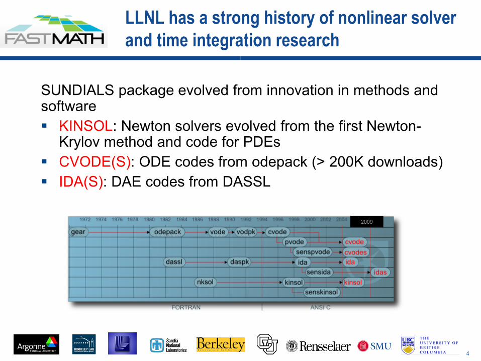
LLNL has a strong history of nonlinear solver and time integration research

SUNDIALS package evolved from innovation in methods and software � KINSOL: Newton solvers evolved from the first Newton-

Krylov method and code for PDEs � CVODE(S): ODE codes from odepack (> 200K downloads) � IDA(S): DAE codes from DASSL

2009

5

� Variable order and variable step size Linear Multistep Methods

� Adams-Moulton (nonstiff); K1 = 1, K2 = k, k = 1, ,12 � Backward Differentiation Formulas [BDF] (stiff); K1 = k, K2 = 0, k = 1, ,5 � Optional stability limit detection based on linear analysis only � The stiff solvers execute a predictor-corrector scheme:

CVODE solves

Explicit predictor to give yn(0)

Implicit corrector with yn(0) as initial iterate

6

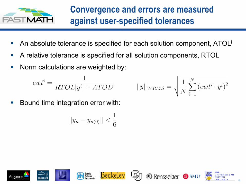
Convergence and errors are measured against user-specified tolerances

� An absolute tolerance is specified for each solution component, ATOLi

� A relative tolerance is specified for all solution components, RTOL

� Norm calculations are weighted by:

� Bound time integration error with:

7

Time steps are chosen to minimize the local truncation error

� Time steps are chosen by: • Estimate the error: E('t ) = C(yn - yn(0))

� Accept step if ||E('t)||WRMS < 1 � Reject step otherwise

• Estimate error at the next step, 't’, as

• Choose next step so that ||E('t’)|| WRMS < 1 � Choose method order by:

• Estimate error for next higher and lower orders • Choose the order that gives the largest time step meeting the

error condition

8

Nonlinear systems at each time step will require nonlinear solves

� Use predicted value as the initial iterate for the nonlinear solver � Nonstiff systems: Functional iteration

� Stiff systems: Newton iteration

ODE

DAE

9

We are adding Runge-Kutta (RK) ODE time integrators to SUNDIALS via ARKode

� RK methods are multistage: allow high order accuracy without long step history (enabling spatial adaptivity)

� Additive RK methods apply a pair of explicit (ERK) and implicit (DIRK) methods to a split system, allowing accurate and stable approximations for multi-rate problems.

� Can decompose the system into “fast” and “slow” components to be treated with DIRK and ERK solvers

� ARKode provides 3rd to 5th order ARK, 2nd to 5th order DIRK and 2nd to 6th order ERK methods; also supports user-supplied methods.

� Implicit RK methods require multiple nonlinear solves per time step � Applies advanced error estimators, adaptive time stepping, Newton

and fixed-point iterative solvers � ARKode will be released with SUNDIALS later this year

http://faculty.smu.edu/reynolds/arkode

10

ARKode solves

� Variable step size additive Runge-Kutta Methods:

� ERK methods use AI=0; DIRK methods use AE=0, � , i = 1,…,s are the inner stage solutions, � is the time-evolved solution, and � is the embedded solution (used for error estimation), � M may be the identity (ODEs) or a non-singular mass matrix (FEM).

11

� If is invertible, we solve for to obtain an ordinary differential equation (ODE), but this is not always the best approach

� Else, the IVP is a differential algebraic equation (DAE)

� A DAE has differentiation index i if i is the minimal number of analytical differentiations needed to extract an explicit ODE

xF �ww / x�

Initial value problems (IVPs) come in the form of ODEs and DAEs

� The general form of an IVP is given by

00 )(0),,(

xtxxxtF

�

12

IDA solves F(t, y, y’) = 0

� C rewrite of DASPK [Brown, Hindmarsh, Petzold] � Variable order / variable coefficient form of BDF (no Adams) � Targets: implicit ODEs, index-1 DAEs, and Hessenberg index-2

DAEs � Optional routine solves for consistent values of y0 and y0’

• Semi-explicit index-1 DAEs • differential components known, algebraic unknown OR • all of y0’ specified, y0 unknown

� Nonlinear systems solved by Newton-Krylov method (no functional iteration)

� Optional constraints: yi > 0, yi < 0, yi t 0, yi d 0

13

CVODE and IDA are equipped with a rootfinding capability

� Finds roots of user-defined functions, gi(t,y) or gi(t,y, y’) � Important in applications where problem definition may change

based on a function of the solution � Roots are found by looking at sign changes, so only roots of odd

multiplicity are found � Checks each time interval for sign change � When sign changes are found, apply a modified secant method with

a tight tolerance to identify root � If gi(t*,y) = 0 for some t*

• gi(t*+G,y) is computed for some small G in direction of integration • Integration stops if any gi(t+G,y) = 0 • Ensures values of gi are nonzero at some past value of t,

beyond which a search for roots is done

14

Sensitivity Analysis

� Sensitivity Analysis (SA) is the study of how the variation in the output of a model (numerical or otherwise) can be apportioned, qualitatively or quantitatively, to different sources of variation in inputs.

� Applications: • Model evaluation (most and/or least influential parameters), Model

reduction, Data assimilation, Uncertainty quantification, Optimization (parameter estimation, design optimization, optimal control, )

� Approaches: • Forward sensitivity analysis – augment state system with sensitivity

equations • Adjoint sensitivity analysis – solve a backward in time adjoint

problem (user supplies the adjoint problem)

15

Adjoint Sensitivity Analysis Implementation

� Solution of the forward problem is required for the adjoint problem Æ need predictable and compact storage of solution values for the solution of the adjoint system

� Cubic Hermite or variable-degree polynomial interpolation � Simulations are reproducible from each checkpoint � Force Jacobian evaluation at checkpoints to avoid storing it � Store solution and first derivative � Computational cost: 2 forward and 1 backward integrations

t0 tf ck0 ck1 ck2

Checkpointing

16

KINSOL solves F(u) = 0

� C rewrite of Fortran NKSOL (Brown and Saad) � Inexact Newton solver: solves J 'un = -F(un) approximately � Modified Newton option (with direct solves) – this freezes the

Newton matrix over a number of iterations � Optional constraints: ui > 0, ui < 0, ui t 0 or ui d 0 � Can scale equations and/or unknowns � Backtracking and line search options for robustness � Dynamic linear tolerance selection for use with iterative linear

solvers

17

Fixed point and Picard iteration will be added to KINSOL in the next release

� Define an iterative scheme to solve F(h) = h - G(h) = 0 as,

� Picard iteration is a fixed point method formed from writing F as the difference of a linear, Lu, and a nonlinear, N(u), operator

� Fixed point iteration has a global but linear convergence theory � Requires G to be a contraction 1,)()( ��d� JJ yxyGxG

end).h(GhSet

)h(F until 0,1,...,k For.h Initialize

k1k

k

0

� �

˱

)()()();()( 11 uGuFLuuNLuNLuuF {� � ��

)()(11 kkkk uGuFLuu �| ��Like Newton with L approximating J

KINSOL will have both Picard and fixed point iterations with acceleration

18

SUNDIALS provides many options for linear solvers

� Iterative Krylov linear solvers • Result in inexact Newton solver • Scaled preconditioned solvers: GMRES, Bi-CGStab, TFQMR • Only require matrix-vector products

• Require preconditioner for the Newton matrix, M � Two options require serial environments and some pre-defined

structure to the data • Direct dense • Direct band

� Jacobian information (matrix or matrix-vector product) can be supplied by the user or estimated with finite difference quotients

19

Our next release of SUNDIALS will include interfaces to sparse direct solvers

� Requires serial vector kernel now – only for transfer of RHS information for Jacobian systems

� Will generalize to more generic vector interface in the future � Matrix information is passed via new SUNDIALS sparse_matrix

structure which utilizes a compressed sparse column format � First release of this capability will support

• SuperLU_MT (multi-threaded version of SuperLU) • KLU (serial)

� Also considering PARDISO (threaded) for future releases

20

Preconditioning is essential for large problems as Krylov methods can stagnate

� Preconditioner P must approximate Newton matrix, yet be reasonably efficient to evaluate and solve.

� Typical P (for time-dep. ODE problem) is � The user must supply two routines for treatment of P:

• Setup: evaluate and preprocess P (infrequently) • Solve: solve systems Px=b (frequently)

� User can save and reuse approximation to J, as directed by the solver

� Band and block-banded preconditioners are supplied for use with the supplied vector structure

� SUNDIALS offers hooks for user-supplied preconditioning • Can use hypre or PETSc or

JJJI |� ~,~J

21

The SUNDIALS vector module is generic

� Data vector structures can be user-supplied � The generic NVECTOR module defines:

• A content structure (void *) • An ops structure – pointers to actual vector operations supplied by

a vector definition � Each implementation of NVECTOR defines:

• Content structure specifying the actual vector data and any information needed to make new vectors (problem or grid data)

• Implemented vector operations • Routines to clone vectors

� Note that all parallel communication resides in reduction operations: dot products, norms, mins, etc.

22

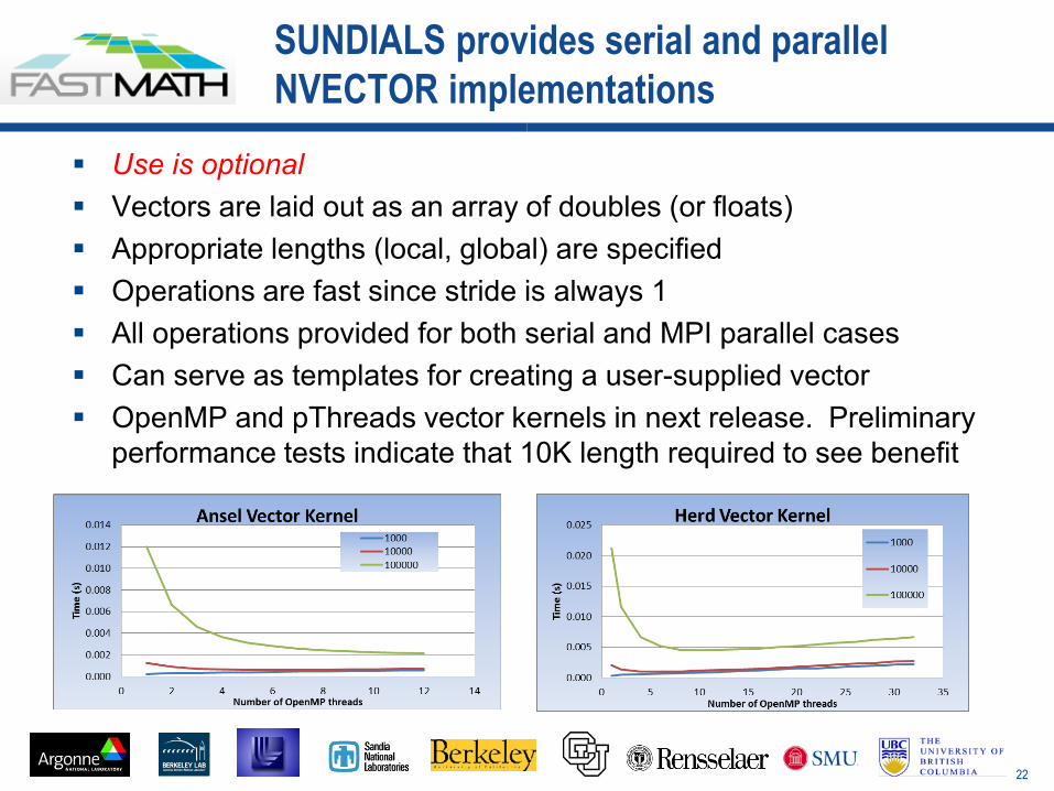
SUNDIALS provides serial and parallel NVECTOR implementations

� Use is optional � Vectors are laid out as an array of doubles (or floats) � Appropriate lengths (local, global) are specified � Operations are fast since stride is always 1 � All operations provided for both serial and MPI parallel cases � Can serve as templates for creating a user-supplied vector � OpenMP and pThreads vector kernels in next release. Preliminary

performance tests indicate that 10K length required to see benefit

23

SUNDIALS provides Fortran interfaces

� CVODE, IDA, and KINSOL � Cross-language calls go in both directions: � Fortran user code ÅÆ interfaces ÅÆ CVODE/KINSOL/IDA

� Fortran main Æ interfaces to solver routines � Solver routines Æ interface to user’s problem-defining routine and

preconditioning routines

� For portability, all user routines have fixed names � Examples are provided

24

SUNDIALS provides Matlab interfaces

� CVODES, KINSOL, and IDAS � The core of each interface is a single MEX file which interfaces to

solver-specific user-callable functions � Guiding design philosophy: make interfaces equally familiar to both

SUNDIALS and Matlab users • all user-provided functions are Matlab m-files • all user-callable functions have the same names as the

corresponding C functions • unlike the Matlab ODE solvers, we provide the more flexible

SUNDIALS approach in which the 'Solve' function only returns the solution at the next requested output time.

� Includes complete documentation (including through the Matlab help system) and several examples

25

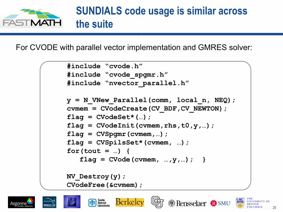
SUNDIALS code usage is similar across the suite

For CVODE with parallel vector implementation and GMRES solver:

#include “cvode.h” #include “cvode_spgmr.h” #include “nvector_parallel.h” y = N_VNew_Parallel(comm, local_n, NEQ); cvmem = CVodeCreate(CV_BDF,CV_NEWTON); flag = CVodeSet*(…); flag = CVodeInit(cvmem,rhs,t0,y,…); flag = CVSpgmr(cvmem,…); flag = CVSpilsSet*(cvmem, …); for(tout = …) { flag = CVode(cvmem, …,y,…); } NV_Destroy(y); CVodeFree(&cvmem);

26

Set/Get routines also customization of solver parameters and output information

Some CVODE optional inputs Set calls

cvmem = CVodeCreate(…); flag = CVodeSet*(cvmem,…); flag = CVodeInit(cvmem,…);

flag = CVSpgmr(cvmem,…); flag = CVSpilsSet*(cvmem, …); flag = CVSpilsSetPreconditioner( cvmem,PrecondSet,PSolve);

Optional Input Function Name Default User data CVodeSetUserData NULL Max. int. order CvodeSetMaxOrd 5 (BDF) Enable stability limit detection

CVodeSetStabLimDet FALSE

Initial step size CVodeSetInitStep Est. Min. step size CVodeSetMinStep 0.0 Max. step size CVodeSetMaxStep infinity Precond. Fcns CVSpilsSet

Preconditioner NULL, NULL

Ratio between lin. & nonlin. tols

CVSpilsSetEpsLin 0.05

Max. Krylov subspace size

CVSpilsSetMaxl 5

27

Example food web problem for KINSOL

A food web population model, with predator-prey interaction and diffusion on the unit square in 2D. The dependent variable vector is the following: and the PDE's are as follows for i = 1, , ns: where The number of species is ns = 2 * np, with the first np being prey and the last np being predators. The coefficients a(i,j), b(i), d(i) are:

= (ଵ, ଶ, ..., ௦)

a(i,i) = -AA, all i; a(i,j) = -GG, i <= np , j > np; a(i,j) = EE, i > np, j <= np b(i) = BB(1 + Dxy), i <= np; b(i) = - BB(1 + Dxy), i > np d(i) = DPREY, i <= np; d(i) = DPRED, i > np

Solved on unit square with �c•n = 0 B.C. and constant initial iterate

28

Example food web problem for KINSOL

#include <kinsol/kinsol.h> #include <kinsol/kinsol_spgmr.h> #include <nvector/nvector_parallel.h> #include <sundials/sundials_dense.h> #include <sundials/sundials_types.h> #include <sundials/sundials_math.h> #include <mpi.h> #define NPEX 2 #define NPEY 2 #define MXSUB 10 #define MYSUB 10 #define MX (NPEX*MXSUB) #define MY (NPEY*MYSUB) #define NEQ (NUM_SPECIES*MX*MY)

/* Type : UserData contains preconditioner blocks, pivot arrays, and problem param */ typedef struct { realtype **P[MXSUB][MYSUB]; long int *pivot[MXSUB][MYSUB]; realtype **acoef, *bcoef; N_Vector rates; realtype *cox, *coy; realtype ax, ay, dx, dy; realtype uround, sqruround; int mx, my, ns, np; realtype cext[NUM_SPECIES * (MXSUB+2)*(MYSUB+2)]; int my_pe, isubx, isuby, nsmxsub, nsmxsub2; MPI_Comm comm; } *UserData;

29

Example food web problem for KINSOL

/* Functions Called by the KINSol Solver */ static int funcprpr(N_Vector cc, N_Vector fval, void *user_data); static int Precondbd(N_Vector cc, N_Vector cscale, N_Vector fval, N_Vector fscale, void *user_data, N_Vector vtemp1, N_Vector vtemp2); static int PSolvebd(N_Vector cc, N_Vector cscale, N_Vector fval, N_Vector fscale, N_Vector vv, void *user_data, N_Vector vtemp);

/* Private Helper Functions */ AllocUserData InitUserData FreeUserData SetInitialProfiles PrintHeader PrintOutput PrintFinalStats WebRate DotProd Bsend BRecvPost BRecvWait ccomm fcalcprpr check_flag

30

Example food web problem for KINSOL

int main(int argc, char *argv[]) { /* Get processor number and total number of pe's */ MPI_Init(&argc, &argv); comm = MPI_COMM_WORLD; MPI_Comm_size(comm, &npes); MPI_Comm_rank(comm, &my_pe); /* Set local vector length */ local_N = NUM_SPECIES*MXSUB*MYSUB; /* Allocate and init. user data*/ data = AllocUserData(); InitUserData(my_pe, comm, data); /* Set global strategy flag */ globalstrategy = KIN_NONE;

/* Allocate and initialize vectors */ cc = N_VNew_Parallel(comm, local_N, NEQ); sc = N_VNew_Parallel(comm, local_N, NEQ); data->rates = N_VNew_Parallel(comm, local_N, NEQ); constraints = N_VNew_Parallel(comm, local_N, NEQ); N_VConst(ZERO, constraints); SetInitialProfiles(cc, sc); fnormtol=FTOL; scsteptol=STOL; /* Call KINCreate/KINInit to initialize KINSOL: A pointer to KINSOL problem memory is returned and stored in kmem. */ kmem = KINCreate();

31

Example food web problem for KINSOL

/* Vector cc passed as template vector. */ flag = KINInit(kmem, funcprpr, cc); flag = KINSetNumMaxIters(kmem, 250); flag = KINSetUserData(kmem, data); flag = KINSetConstraints(kmem, constraints); flag = KINSetFuncNormTol(kmem, fnormtol); flag = KINSetScaledStepTol(kmem, scsteptol); /* We no longer need the constraints vector since KINSetConstraints creates a private copy for KINSOL to use. */ N_VDestroy_Parallel(constraints);

/* Call KINSpgmr to specify the linear solver KINSPGMR with preconditioner routines Precondbd and PSolvebd, and the pointer to the user data block. */ maxl = 20; maxlrst = 2; flag = KINSpgmr(kmem, maxl); flag = KINSpilsSetMaxRestarts(kmem, maxlrst); flag = KINSpilsSetPreconditioner(kmem, Precondbd, PSolvebd);

32

Example food web problem for KINSOL

/* Call KINSol and print output profile */ flag = KINSol(kmem, /* KINSol memory*/ cc, /* initial guess input; sol’n output*/ globalstrategy, /* nonlinear strategy*/ sc, /* scaling vector for variable cc */ sc); /* scaling vector for function vals*/ /* Print final statistics and free memory */ if (my_pe == 0) PrintFinalStats(kmem); N_VDestroy_Parallel(cc); N_VDestroy_Parallel(sc); KINFree(&kmem); FreeUserData(data); MPI_Finalize(); return(0); }

33

SUNDIALS has been used worldwide in applications from research and industry

� Power grid modeling (RTE France, ISU)

� Simulation of clutches and power train parts (LuK GmbH & Co.)

� Electrical and heat generation within battery cells (CD-adapco)

� 3D parallel fusion (SMU, U. York, LLNL) � Implicit hydrodynamics in core collapse

supernova (Stony Brook) � Dislocation dynamics (LLNL) � Sensitivity analysis of chemically reacting flows

(Sandia)

� Large-scale subsurface flows (CO Mines, LLNL)

� Optimization in simulation of energy-producing algae (NREL)

� Micromagnetic simulations (U. Southampton)

Magnetic reconnection

Core collapse supernova

Dislocation dynamics

Subsurface flow

More than 3,500 downloads each year

34

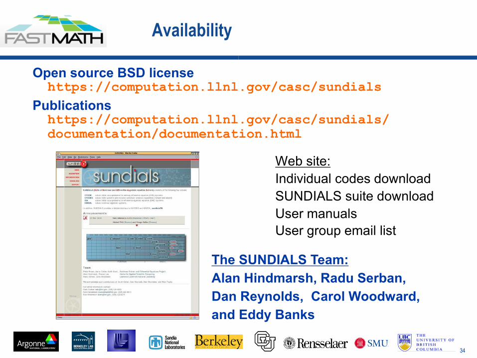
Availability

Web site: Individual codes download SUNDIALS suite download User manuals User group email list

The SUNDIALS Team: Alan Hindmarsh, Radu Serban, Dan Reynolds, Carol Woodward, and Eddy Banks

Open source BSD license https://computation.llnl.gov/casc/sundials

Publications https://computation.llnl.gov/casc/sundials/documentation/documentation.html