Sums Of Squares For Power Systems Transient Stability Analysis · 2018-01-17 · Introduction Our...
72
Introduction Our Power System Theoretical Tools Transient Stability Analysis Conclusion Sums Of Squares For Power Systems Transient Stability Analysis Master project at RTE-ECN International chair in automatic control and power grids Matteo Tacchi PhD student at LAAS-CNRS / RTE-R&D January 17, 2018
Transcript of Sums Of Squares For Power Systems Transient Stability Analysis · 2018-01-17 · Introduction Our...

Introduction Our Power System Theoretical Tools Transient Stability Analysis Conclusion
Sums Of Squares For Power Systems TransientStability Analysis
Master project at RTE-ECN International chair in automaticcontrol and power grids
Matteo Tacchi
PhD student at LAAS-CNRS / RTE-R&D
January 17, 2018

Introduction Our Power System Theoretical Tools Transient Stability Analysis Conclusion
Outline
1 Our Power System
2 Theoretical Tools
3 Transient Stability Analysis

Introduction Our Power System Theoretical Tools Transient Stability Analysis Conclusion
Introduction
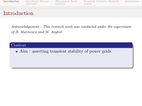
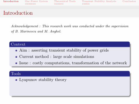
Acknowledgement : This research work was conducted under the supervision
of B. Marinescu and M. Anghel.
Context
Aim : asserting transient stability of power grids
Current method : large scale simulations
Issue : costly computations, transformation of the network
Tools
Lyapunov stability theory
Real algebraic geometry : Positivstellensatz
Sum-Of-Squares / Semidefinite Programming
Introduction Our Power System Theoretical Tools Transient Stability Analysis Conclusion
Introduction
Acknowledgement : This research work was conducted under the supervision
of B. Marinescu and M. Anghel.
Context
Aim : asserting transient stability of power grids
Current method : large scale simulations
Issue : costly computations, transformation of the network
Tools
Lyapunov stability theory
Real algebraic geometry : Positivstellensatz
Sum-Of-Squares / Semidefinite Programming

Introduction Our Power System Theoretical Tools Transient Stability Analysis Conclusion
Background
[Anghel, Milano & Papachristodoulou] Algorithmic construction ofLyapunov functions for power system stability analysis. 2013.
G1
G2
R12 + jX12 R23 + jX23
R13 + jX13G3
Our contribution
Here : no regulation =⇒ accurate but narrow stability regionWe implement the method on a regulated system with only 2 machinesWider stability region expected, computations more difficult

Introduction Our Power System Theoretical Tools Transient Stability Analysis Conclusion
Background
[Anghel, Milano & Papachristodoulou] Algorithmic construction ofLyapunov functions for power system stability analysis. 2013.
G1
G2
R12 + jX12 R23 + jX23
R13 + jX13G3
Our contribution
Here : no regulation =⇒ accurate but narrow stability region
We implement the method on a regulated system with only 2 machinesWider stability region expected, computations more difficult

Introduction Our Power System Theoretical Tools Transient Stability Analysis Conclusion
Background
[Anghel, Milano & Papachristodoulou] Algorithmic construction ofLyapunov functions for power system stability analysis. 2013.
G1
G2
R12 + jX12 R23 + jX23
R13 + jX13G3
Our contribution
Here : no regulation =⇒ accurate but narrow stability regionWe implement the method on a regulated system with only 2 machines
Wider stability region expected, computations more difficult

Introduction Our Power System Theoretical Tools Transient Stability Analysis Conclusion
Background
[Anghel, Milano & Papachristodoulou] Algorithmic construction ofLyapunov functions for power system stability analysis. 2013.
G1
G2
R12 + jX12 R23 + jX23
R13 + jX13G3
Our contribution
Here : no regulation =⇒ accurate but narrow stability regionWe implement the method on a regulated system with only 2 machinesWider stability region expected, computations more difficult

Introduction Our Power System Theoretical Tools Transient Stability Analysis Conclusion
Outline
1 Our Power System
2 Theoretical Tools
3 Transient Stability Analysis

Introduction Our Power System Theoretical Tools Transient Stability Analysis Conclusion
The Nominal System
System Description
G
SR+ jX R+ jX
2(R+ jX)
N∞
VG ∼ (vd, vq) V∞ = Vsejωst
∞

Introduction Our Power System Theoretical Tools Transient Stability Analysis Conclusion
The Nominal System
Our Model
Nominal Equations
[Sauer & Pai] Power System Dynamics and Stability. Prentice Hall, 1998.
T ′d0 e
′q = −e′q − (xd − x′d)id + Efd
2Hω = Pm − (vdid + vqiq + ri2d + ri2q)
δ = ω − ωsvd = Rid −Xiq + Vs sin(δ)
vq = Riq +Xid + Vs cos(δ)
−Vs sin(δ) = (R+ r)id − (X + xq)iq
e′q − Vs cos(δ) = (R+ r)iq + (X + x′d)id
Ta ˙Efd = −Efd +Ka
(Vref −
√v2d + v2
q
)Tg ˙Pm = −Pm + Pref +Kg(ωref − ω)

Introduction Our Power System Theoretical Tools Transient Stability Analysis Conclusion
The Nominal System
Our Model
Nominal Equations
[Sauer & Pai] Power System Dynamics and Stability. Prentice Hall, 1998.
T ′d0 e
′q = −e′q − (xd − x′d)id + Efd
2Hω = Pm − (vdid + vqiq + ri2d + ri2q)
δ = ω − ωs
vd = Rid −Xiq + Vs sin(δ)
vq = Riq +Xid + Vs cos(δ)
−Vs sin(δ) = (R+ r)id − (X + xq)iq
e′q − Vs cos(δ) = (R+ r)iq + (X + x′d)id
Ta ˙Efd = −Efd +Ka
(Vref −
√v2d + v2
q
)Tg ˙Pm = −Pm + Pref +Kg(ωref − ω)

Introduction Our Power System Theoretical Tools Transient Stability Analysis Conclusion
The Nominal System
Our Model
Nominal Equations
[Sauer & Pai] Power System Dynamics and Stability. Prentice Hall, 1998.
T ′d0 e
′q = −e′q − (xd − x′d)id + Efd
2Hω = Pm − (vdid + vqiq + ri2d + ri2q)
δ = ω − ωsvd = Rid −Xiq + Vs sin(δ)
vq = Riq +Xid + Vs cos(δ)
−Vs sin(δ) = (R+ r)id − (X + xq)iq
e′q − Vs cos(δ) = (R+ r)iq + (X + x′d)id
Ta ˙Efd = −Efd +Ka
(Vref −
√v2d + v2
q
)Tg ˙Pm = −Pm + Pref +Kg(ωref − ω)

Introduction Our Power System Theoretical Tools Transient Stability Analysis Conclusion
The Nominal System
Our Model
Nominal Equations
[Sauer & Pai] Power System Dynamics and Stability. Prentice Hall, 1998.
T ′d0 e
′q = −e′q − (xd − x′d)id + Efd
2Hω = Pm − (vdid + vqiq + ri2d + ri2q)
δ = ω − ωsvd = Rid −Xiq + Vs sin(δ)
vq = Riq +Xid + Vs cos(δ)
−Vs sin(δ) = (R+ r)id − (X + xq)iq
e′q − Vs cos(δ) = (R+ r)iq + (X + x′d)id
Ta ˙Efd = −Efd +Ka
(Vref −
√v2d + v2
q
)Tg ˙Pm = −Pm + Pref +Kg(ωref − ω)

Introduction Our Power System Theoretical Tools Transient Stability Analysis Conclusion
The Perturbation
Introduction of a Short-circuit
Short-circuit Protocol
1) Start from nominal operating system at equilibrium
2) at t = tc, a short-circuit occurs : the state is not atequilibrium anymore
3) at t = tcl = tc + ∆t, the short-circuit is eliminated (back tonominal equations : successful auto-reclosing)
Question : What is the critical clearing time (CCT ) i.e. themaximal value of ∆t such that the system reaches anequilibrium point after the fault elimination ?

Introduction Our Power System Theoretical Tools Transient Stability Analysis Conclusion
The Perturbation
The Short-circuited System
G
SR+ jX R+ jX
2(R+ jX)
N∞
VG ∼ (vd, vq) V∞ = Vsejωst
∞

Introduction Our Power System Theoretical Tools Transient Stability Analysis Conclusion
The Perturbation
The Short-circuited System
Short-circuit Equations
T ′d0 e
′q = −e′q − (xd − x′d)id + Efd
2Hω = Pm − (vdid + vqiq + ri2d + ri2q)
δ = ω − ωs
3vd = 2Rid − 2Xiq + Vs sin(δ)
3vq = 2Riq + 2Xid + Vs cos(δ)
−Vs sin(δ) = (2R+ 3r)id − (2X + 3xq)iq
3e′q − Vs cos(δ) = (2R+ 3r)iq + (2X + 3x′d)id
Ta ˙Efd = −Efd +Ka
(Vref −
√v2d + v2
q
)Tg ˙Pm = −Pm + Pref +Kg(ωref − ω)

Introduction Our Power System Theoretical Tools Transient Stability Analysis Conclusion
The Perturbation
The Short-circuited System
Short-circuit Equations
T ′d0 e
′q = −e′q − (xd − x′d)id + Efd
2Hω = Pm − (vdid + vqiq + ri2d + ri2q)
δ = ω − ωs3vd = 2Rid − 2Xiq + Vs sin(δ)
3vq = 2Riq + 2Xid + Vs cos(δ)
−Vs sin(δ) = (2R+ 3r)id − (2X + 3xq)iq
3e′q − Vs cos(δ) = (2R+ 3r)iq + (2X + 3x′d)id
Ta ˙Efd = −Efd +Ka
(Vref −
√v2d + v2
q
)Tg ˙Pm = −Pm + Pref +Kg(ωref − ω)

Introduction Our Power System Theoretical Tools Transient Stability Analysis Conclusion
Preliminary Computations
Equilibrium Point
The state variables δ, ω, e′q, Efd and Pm remain constant whenthey reach the value
δeq = 1.579ωeq = 1
e′eqq = 1.055Eeqfd = 2.477
P eqm = 0.7
This equilibrium point is LAS (according to the simulations).

Introduction Our Power System Theoretical Tools Transient Stability Analysis Conclusion
Preliminary Computations
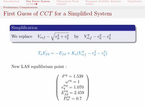
First Guess of CCT for a Simplified System
Simplification
We replace Vref −√v2d + v2
q by V 2ref − v2
d − v2q
Ta ˙Efd = −Efd +Ka(V2ref − v2
d − v2q )
New LAS equilibrium point :δeq = 1.539ωeq = 1
e′eqq = 1.070Eeqfd = 2.459
P eqm = 0.7
Introduction Our Power System Theoretical Tools Transient Stability Analysis Conclusion
Preliminary Computations
First Guess of CCT for a Simplified System
Simplification
We replace Vref −√v2d + v2
q by V 2ref − v2
d − v2q
Ta ˙Efd = −Efd +Ka(V2ref − v2
d − v2q )
New LAS equilibrium point :δeq = 1.539ωeq = 1
e′eqq = 1.070Eeqfd = 2.459
P eqm = 0.7

Introduction Our Power System Theoretical Tools Transient Stability Analysis Conclusion
Preliminary Computations
First Guess of CCT for a Simplified System
Simplification
We replace Vref −√v2d + v2
q by V 2ref − v2
d − v2q
∆t = 4.057s ∆t = 4.058s

Introduction Our Power System Theoretical Tools Transient Stability Analysis Conclusion
Outline
1 Our Power System
2 Theoretical Tools
3 Transient Stability Analysis

Introduction Our Power System Theoretical Tools Transient Stability Analysis Conclusion
Notions of Stability
Definition : Transient Stability
Transient Stability denotes the ability of a power system’sangular characteristics to return to operating equilibrium andsychronism after a large disturbance, and within a shortamount of time (under 10s), usually going through a first-swingaperiodic drift.
Definition : A case of Lyapunov Stability
A solution x ∈ Rn to the equation F (x) = 0 is an equilibriumpoint of the system
x = F (x). (1)
It is said to be locally asymptotically stable (LAS) iff it admitsa Region Of Attraction (ROA) s.t.
x(0) ∈ ROA =⇒ x(t) −→t→+∞
x.

Introduction Our Power System Theoretical Tools Transient Stability Analysis Conclusion
Notions of Stability
Theorem [Lyapunov - Massera]
x = 0 is a LAS equilibrium point of the previous system iff∃V : D ⊂ Rn −→ R s.t. V (0) = 0 &
x 6= 0 =⇒ V (x) > 0, V (x) := ∇V (x) · F (x) < 0
Then, any Ωc := x ∈ Rn | V (x) ≤ c s.t. Ωc ⊂ D is a positivelyinvariant subset of the ROA.

Introduction Our Power System Theoretical Tools Transient Stability Analysis Conclusion
The Positivstellensatz
Some Useful Objects
Definition : Algebraic Structures
Let G = (g1, . . . , gβ),F = (f1, . . . , fα),H = (h1, . . . , hγ) ∈ Rn.
Multiplicative Monoid generated by G
M(G) :=
β∏j=1
gkjj | k1, . . . , kβ ∈ N
Quadratic Module generated by F
P(F) :=
s0 +
α∑i=1
sifi | s0, . . . , sα ∈ Σn
Ideal generated by H
I(H) :=
γ∑i=1
hkpk | p1, . . . , pγ ∈ Rn

Introduction Our Power System Theoretical Tools Transient Stability Analysis Conclusion
The Positivstellensatz
Some Useful Objects
Definition : Algebraic Structures
Let G = (g1, . . . , gβ),F = (f1, . . . , fα),H = (h1, . . . , hγ) ∈ Rn.Multiplicative Monoid generated by G
M(G) :=
β∏j=1
gkjj | k1, . . . , kβ ∈ N
Quadratic Module generated by F
P(F) :=
s0 +
α∑i=1
sifi | s0, . . . , sα ∈ Σn
Ideal generated by H
I(H) :=
γ∑i=1
hkpk | p1, . . . , pγ ∈ Rn

Introduction Our Power System Theoretical Tools Transient Stability Analysis Conclusion
The Positivstellensatz
The Positivstellensatz
[Bochnak, Coste & Roy] Geometrie Algebrique Reelle. Springer, 1986.
Theorem [P-satz]
The set f1(x) ≥ 0, . . . , fα(x) ≥ 0x ∈ Rn g1(x) 6= 0, . . . , gβ(x) 6= 0
h1(x) = 0, . . . , hγ(x) = 0
is empty iff ∃f ∈ P(F), g ∈M(G), h ∈ I(H) ;
f + g2 + h = 0. (2)

Introduction Our Power System Theoretical Tools Transient Stability Analysis Conclusion
The Expanding Interior Algorithm
Mixing Lyapunov theory and P-satz to find the ROA
[Wloszek] Lyapunov based analysis and controller synthesis forpolynomial systems using SOS optimization. PhD, 2003.
Estimation of the ROA
x = F (x), F ∈ Rn, 0 LAS equilibrium point.Tool to estimate 0’s ROA : V ∈ Rn s.t.
V (0) = 0 & x 6= 0 =⇒ V (x) > 0
V (x) < 0 on D \ 0, D := x ∈ Rn | V (x) ≤ 1

Introduction Our Power System Theoretical Tools Transient Stability Analysis Conclusion
The Expanding Interior Algorithm
Mixing Lyapunov theory and P-satz to find the ROA
How do we obtain a “good” estimation ?
Aim : maximize the size of D ⊂ ROA (according toLyapunov theory)
Method : maximize the size of somePβ := x | p(x) ≤ β ⊂ D with p ∈ Σn positive definite(e.g. p(x) = ‖x‖2)
Practical implementation : maximize β.

Introduction Our Power System Theoretical Tools Transient Stability Analysis Conclusion
The Expanding Interior Algorithm
Mixing Lyapunov theory and P-satz to find the ROA
Resulting set emptiness problem
maxV ∈Rn,V (0)=0
β s.t.
x ∈ Rn| − V (x) ≥ 0, ε‖x‖2 6= 0 = ∅x ∈ Rn|β − p(x) ≥ 0, V (x)− 1 ≥ 0, V (x)− 1 6= 0 = ∅
x ∈ Rn|1− V (x) ≥ 0, V (x) ≥ 0, ε‖x‖2 6= 0 = ∅
Equivalent SOS problem using P-satz
maxV ∈Rn,V (0)=0k1,k2,k3∈N∗
s1,...,s10∈Σn
β s.t.
s1 − V s2 + ε‖ · ‖4k1 = 0s3 + (β − p)s4 + (V − 1)s5 + (β − p)(V − 1)s6 + (V − 1)2k2 = 0s7 + (1− V )s8 + V s9 + (1− V )V s10 + ε‖ · ‖4k3 = 0

Introduction Our Power System Theoretical Tools Transient Stability Analysis Conclusion
The Expanding Interior Algorithm
Mixing Lyapunov theory and P-satz to find the ROA
Resulting simplified SOS problem
maxV ∈Rn,V (0)=0s6,s8,s9∈Σn
β s.t.
V − ε‖ · ‖2 =: s1 ∈ Σn
− ((β − p)s6 + (V − 1)) =: s5 ∈ Σn (3)
−(
(1− V )s8 + V s9 + ε‖ · ‖2)
=: s7 ∈ Σn

Introduction Our Power System Theoretical Tools Transient Stability Analysis Conclusion
The Expanding Interior Algorithm
Expanding Interior Algorithm
A bilinear program
The issue with the SOS problem we obtain is that we want tooptimize β with V and the si as variables.=⇒ we are faced to a bilinear program (and not a linearprogram that we know how to solve)
An algorithmic solution
The EIA tackles the maximization of β by iterating two distinctsteps :
First linear search while V is fixed and the si vary
Second linear search while V and s6 vary and the other siare fixed

Introduction Our Power System Theoretical Tools Transient Stability Analysis Conclusion
Outline
1 Our Power System
2 Theoretical Tools
3 Transient Stability Analysis
Introduction Our Power System Theoretical Tools Transient Stability Analysis Conclusion
Reduction to a polynomial system
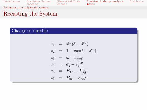
Recasting the System
Change of variable
z1 = sin(δ − δeq)z2 = 1− cos(δ − δeq)z3 = ω − ωrefz4 = e′q − e′,eqq
z5 = Efd − Eeqfdz6 = Pm − Pref
Constraint G(z) = z21 + z2
2 − 2z2 = 0
z = H(z), with H ∈ Rn and H(0) = 0

Introduction Our Power System Theoretical Tools Transient Stability Analysis Conclusion
Reduction to a polynomial system
Resulting Expanding Interior ProgramSet emptiness problem
maxV ∈Rn,V (0)=0
β s.t.
z ∈ R6| − V (z) ≥ 0, ε‖z‖2 6= 0, G(z) = 0 = ∅z ∈ R6|β − p(z) ≥ 0, V (z)− 1 ≥ 0, V (z)− 1 6= 0, G(z) = 0 = ∅
z ∈ R6|1− V (z) ≥ 0, V (z) ≥ 0, ε‖z‖2 6= 0, G(z) = 0 = ∅
SOS problem
maxV ,q1,q2,q3∈Rn,V (0)=0
s6,s8,s9∈Σn
β s.t.
V − ε‖ · ‖2 − q1G =: s1 ∈ Σn
− ((β − p)s6 + (V − 1))− q2G =: s5 ∈ Σn (4)
−(
(1− V )s8 + V s9 + ε‖ · ‖2)− q3G =: s7 ∈ Σn

Introduction Our Power System Theoretical Tools Transient Stability Analysis Conclusion
Our results
Plot of the estimated ROA
δmax = δeq + 0.743puωmax = ωref + 0.209pu

Introduction Our Power System Theoretical Tools Transient Stability Analysis Conclusion
Our results
Plot of the estimated ROA
e′q,max = e′eqq + 0.496puEfd,max = Eeq
fd + 14.72puPm,max = Pref + 2.029pu

Introduction Our Power System Theoretical Tools Transient Stability Analysis Conclusion
Our results
Plot of the resulting Lyapunov function V
CCT estimate : CCT = 3.591sactual CCT : CCT = 4.057s

Introduction Our Power System Theoretical Tools Transient Stability Analysis Conclusion
Our results
Comparison to the actual ROA
ωinit = 1.2011pu ωinit = 1.2012pu
Variable δ ω e′q Efd Pm
Actual R.O.A.’s upper bound 2.465 1.211 2.966 95.42 3.888
R.O.A. estimate’s upper bound 2.282 1.209 1.566 17.18 2.729

Introduction Our Power System Theoretical Tools Transient Stability Analysis Conclusion
Conclusion
[Tacchi, Marinescu, Anghel, Kundu, Benahmed & Cardozo]Power systems transient stability analysis using SOS programming.Submitted to Power Systems Computation Conference in october 2017.
A wider ROA
As expected the ROA and its estimation are larger with regulations
Possible further developments
Implement the same method with a better scaled polynomial p = Vend
Solve the problem with the actual voltage regulation (nosimplification)
Solve the problem using the method proposed in [Korda, Henrion &Jones] Inner approximations of the region of attraction for polynomialdynamical systems
Tackle power grids with a well-formulated sparse moment-SOShierarchy (exploiting the network structure)

Introduction Our Power System Theoretical Tools Transient Stability Analysis Conclusion
Thank you for your attention.Questions are welcome !