Summer Paper - Terrence Adam Rooney

A Game-Theoretic Analysis of a Poker Hand

Terrence Adam Rooney1

September 30, 2016

Abstract

This paper presents a model motivated by the first betting round in a single, two -

player, No-Limit Hold’em poker hand. In this model, the two, risk-neutral, players

engage in a static, simultaneous-move game of incomplete information that

incorporates luck along with technical and perceptive skill. Through a comparative

static analysis, I develop insights regarding the parametric effects of the model.

Through this analysis, the insights I reveal are consistent with conventional poker

wisdom and the results obtained by other works of literature.

1 I would like to thank Professor Peter Streufert for the insight he has provided to me throughout the development of this paper. I would also l ike to thank Professor Gregory Pavlov, along with my classmates, Minku Kang and

Shannon Potter, for their helpful comments.

1 Introduction & Related Literature

As the internet grew to prominence in the early 21st century, many industries

were revolutionized and, consequently, experienced a drastic change in prevalence

and popularity. The poker industry was no exception. After Chris Moneymaker, a

professional accountant and amateur online poker player, won the 2003 World Series

of Poker “WSOP” Main Event, the number of entrants in this tournament grew from

839 in 2003 to 5,619 in 2005 (Croson et al., 2008). People rationalize that, if Chris

Moneymaker could qualify online for the WSOP Main Event and win, then anyone

can do so (McCormack & Griffiths, 2012). Over the past decade, the large number of

entries to this World Championship tournament has persisted, with the most recent

event drawing a field of 6,737 players (“WSOP.com”, 2016). Additionally, it is

estimated that approximately eighty million people (over 1 percent of the global

population) play poker on a regular basis (Holden, 2008).

Despite the significant growth in popularity that poker has experienced, very

little empirical research regarding online poker has been conducted (Griffiths et al.,

2010). However, there have been various attempts to theoretically devise an optimal

poker strategy. Burns (2004) examines the roles of style and skill in a simplified poker

game, and shows that the best style for one player depends on the style of her

opponent. Burns (2004) also demonstrates, in his model, that Novice styles can be

remarkably effective against Expert skill. Although initially unintuitive, the logic

behind this conjecture is based on the fact that an expert poker player is able to

capitalize on predicting their opponent’s behaviour, and hence gains a competitive

advantage. But, when an expert player is facing a novice opponent that does not know

how to optimally, or even skillfully, play their hand, the expert’s advantage is

mitigated since the novice’s approach will be more random and unpredictable than

that of a moderately skilled player.

Dreef et al. (2004) also attempt to devise an optimal poker strategy by

providing an overview of the relevant aspects of a method, presented by Borm and

Van der Genugten (2000, 2001), that determines whether a game can be classified as

a game of skill or not. Dreef et al. (2004) utilize a simple, two-person poker game to

illustrate the concepts presented in their paper. However, they still have some

difficulty with incorporating skill concepts in game theory (McCormack, A., &

Griffiths, 2012). The model that I present in this paper also features a simple, two-

person poker game, similar to that which is contained in Dreef et al. (2004). Both of

our models assume that players of a higher ability have better information than their,

lesser-skilled, counterpart. My paper, however, will split a player’s skill into two

ability components, informational (technical) and perceptive, whereas Dreef et al.

(2004) assumes that players only differ in their informational (technical) skill.

Another critical difference between our models is that Dreef et al. (2004) features a

sequential-move game, whereas my model presents a simultaneous-move game.

Although, in reality, poker is a sequential-move game, I have chosen to implement a

simultaneous-move structure since it presents the possibility of applying my results

to many real-world situations, such as entrepreneurs (or firms) entering an industry

and job-seekers searching for employment. I will address these applications, among

others, in a future paper, and have decided, here, to limit my focus to presenting my

model and conducting a comparative static analysis on each of the model’s features.

Poker has been researched in many fields of study, such as computer science,

economics, psychology, and statistics, with the majority of academic research taking

place in fields outside of economics. For instance, works from the computer science

field include Billings et al. (2002, 2003), Korb et al. (1999), Shi & Littman (2000), and

Southey et al. (2012); works from the psychology field include Griffiths et al. (2010),

McCormack & Griffiths (2012), and Rapoport et al. (1997); and works from the

statistics field include Borm and Van der Genugten (2000, 2001), and Crosen et al.,

(2008).

Research papers that have linked economics with poker primarily fall within

the field of Behavioral Economics or focus on the empirical relationship between luck

and skill. Siler (2010) analyzes poker hands played online in small, medium, and high

stakes, then determines which strategies are conducive to winning at each level.

Consequently, Siler (2010) finds that a skillful player’s competitive edge diminishes

as she moves up levels, while at the same time, tight-aggressive strategies, which

tend to be the most lucrative, become more prevalent.

Levitt & Miles (2014) apply data from the 2010 WSOP to shed insight on

whether poker is a game of luck or skill. Their results provide strong evidence that

supports the idea that poker is a game of skill. This is because, in their study, players

identified as highly skilled prior to the start of the 2010 WSOP finished with a return

on investment of over 30%, whereas all other players combined achieved a -15%

return on investment. Hannum & Cabot (2009) arrive at a similar result as Levitt &

Miles (2014), in the sense that they also find that poker is predominately a game of

skill. To reach this conclusion, Hannum & Cabot (2009) run a mathematically-based

simulation study that demonstrates the payout benefits for a player that employs a

skillful strategy versus the drawbacks for a player utilizing a randomized (unskilled)

strategy. Contrarily, Meyer et al. (2013) finds that poker, under basic conditions,

should be regarded as a game of chance, since their findings indicate that the

outcomes of poker games are predominantly determined by chance. Meyer et al.

(2013) arrive at this conjecture by completing a quasi-experimental study that

examines the extent to which poker skill was more important than the distribution

of cards dealt. Upon taking this all into consideration, it is clear that the luck versus

skill debate with poker has yet to be settled.

Although the model that I feature in this paper is meant to replicate a

simplified poker game, it has various similarities to other theoretical models and

concepts detailed in economics literature. Haltiwanger & Waldman (1985)

investigates a model that emphasizes heterogeneity between agents that vary in

terms of informational processing ability. They find that in an environment

characterized by congestion effects (i.e. the higher the number of agents choosing a

strategy, the worse off each corresponding agent is), informationally-skilled agents

have a disproportionally large effect on equilibrium. Their findings also indicate that

in an environment characterized by synergistic effects, naïve agents tend to be

disproportionally important. Aumann & Heifetz (2002) acknowledges the importance

of incorporating a player’s beliefs about the other players’ beliefs into game theoretic

models, and it also details various ways of doing this. Finally, Jehiel & Koessler

(2008) studies the effects of analogy-based expectations in static two-player games of

incomplete information. Their paper assumes that players only understand the

average behaviour of their opponent over bundles of states, then characterizes

players by how finely they understand the strategy of their opponent together with

their own information and payoff structure.

Finally, in addition to the above research, a related stream of economics

literature is that of overconfidence, and other personality traits, in contests. Ando

(2004) investigates an economic contest featuring two players who are each

overconfident in their own relative abilities. Specifically, Ando (2004) studies two

different sources of overconfidence, a player’s overestimation of their own ability and

a player’s underestimation of their opponent’s ability. He finds, in his paper, that a

player’s overestimation of their own ability leads to that player exhibiting aggressive

behaviour, whereas a player’s underestimation of their opponents’ ability sometimes

leads to less aggressive behaviour by one or both players. Therefore, according to this

result, overconfidence may not always lead to aggressive play. Ludwig et al. (2011)

utilize a model that incorporates a two-player Tullock contest to show that modest

overconfidence in a contest can improve a player’s performance relative to an

unbiased opponent, and possibly lead to an absolute advantage for the overconfident

player. Finally, through an experimental study, Alaoui & Fons-Rosen (2016)

examines how grit, which is linked to perseverance, influences behaviour. They show

that along with this commonly known upside of grit, there is also a potential downside

in the form stubbornness.

The remainder of my paper is as follows. Section 2 presents the motivation

behind my model. Section 3 details the model. Section 4 explains the parameters that

I have chosen for the model’s benchmark case. Section 5 presents the analysis, and

Section 6 concludes.

2 Motivation

The model I will present is motivated by the first betting round of a single, two-

player, hand of No-Limit Hold’em poker. In a standard hand, players are each dealt

two cards, and are endowed with a set number of chips (i.e. capital). In order to

incentivize betting, players are obligated to pay blinds into the pot. Players then

proceed through playing the hand2.

A common occurrence in tournament poker is when the blinds are large in

relation to each player’s number of chips. When this happens, a popular strategy , in

the first betting round, for players is to either fold their hand and relinquish the blind

they have paid into the pot, or raise (henceforth known as call) all of their chips and

put maximum pressure on their opponent to fold, which would result in the player

winning the blind of their opponent. With this in mind, I have decided to conduct

analysis based on the assumption that each player can choose one of only these two

actions.

2 Please refer to “Texas Hold’em Rules” (2016) for an overview of how a poker hand is played.

3 Model

I consider a model that features two, risk-neutral, players engaging in a static,

simultaneous-move game of incomplete information. Each player (𝑖 ∈ {1, 2}) is

endowed with an initial level of capital, 𝑘𝑖0, and there exists a blind cost (𝑏) such that

𝑏 ∈ (0,𝑀𝑖𝑛{𝑘10,𝑘2

0}]. Each player (𝑖 ∈ {1, 2}) is endowed with an informational ability

coordinate, (𝑥𝑖 ,𝑦𝑖), that satisfies the following constraints:

𝑥𝑖 ∈ [0,1] and 𝑦𝑖 ∈ [0,1] (1) − "𝐵𝑜𝑢𝑛𝑑𝑎𝑟𝑦"

1

2(1 − 𝑥𝑖) + 𝑦𝑖 ≤ 1 (2) − "𝑁𝑒𝑔𝑎𝑡𝑖𝑣𝑖𝑡𝑦"

4𝑦𝑖 − 𝑥𝑖 ≥ 1 (3) − "𝐸𝑥𝑝𝑒𝑐𝑡𝑒𝑑 𝑉𝑎𝑙𝑢𝑒"

Additionally, each player (𝑖 ∈ {1, 2}) is assigned a perceptive ability3 𝑝𝑖 ∈ {1,4}.

3.1 Timeline

The timeline for this game is as follows. For each player (𝑖 ∈ {1, 2}), Nature

draws, with equal probability, a hand-type, 𝑐𝑖 ∈ {1, 2, 3}, as well as a lottery-type, Λ𝑖 ∈

{𝐿1(𝑥𝑖 ,𝑦𝑖),𝐿2(𝑥𝑖 ,𝑦𝑖),𝐿 3(𝑥𝑖 ,𝑦𝑖)}. Each player (𝑖 ∈ {1, 2}) observes their own abilities,

lottery-type, capital values, blind cost, their opponent’s perceptive ability, and if 𝑝𝑖 =

1, their opponent’s informational ability. Upon making these observations, each

player (𝑖 ∈ {1,2}) chooses an action, 𝑎𝑖(Λ𝑖), such that 𝑎𝑖(Λ𝑖) ∈ {Fold, Call}4. For 𝑖 ∈

{1, 2}, if player 𝑖 chooses “Fold”, the blind cost (𝑏) is deducted from player 𝑖′𝑠 capital,

3 Both ability types for player 𝑖 (𝑖 ∈ {1, 2}) are independent of each other. Additionally, each ability type for player

𝑖 is independent of the ability types endowed to player −𝑖. 4 In the Analysis section, “Fold” will be denoted as “F”, and “Call” will be denoted as “C”.

and added to player −𝑖′𝑠 capital (𝑖.𝑒. ∶ 𝑘𝑖 = 𝑘𝑖0 − 𝑏 & 𝑘−𝑖 = 𝑘−𝑖

𝑜 + 𝑏). If both players

choose “Call”, then the following showdown occurs. For 𝑖 ∈ {1,2}, Nature draws three

additional values, 𝛼𝑖 , 𝛽𝑖 , 𝛾𝑖 ∈ {1,2, 3}5. Subsequently, for 𝑖 ∈ {1, 2}, the capital values

update as follows:

𝑘𝑖 = {

𝑘𝑖0 + 𝑀𝑖𝑛{𝑘𝑖

0, 𝑘−𝑖0 } 𝑖𝑓 𝑐𝑖 + 𝜆𝑖 > 𝑐−𝑖 + 𝜆−𝑖

𝑘𝑖0 − 𝑀𝑖𝑛{𝑘𝑖

0, 𝑘−𝑖0 } 𝑖𝑓 𝑐𝑖 + 𝜆𝑖 < 𝑐−𝑖 + 𝜆−𝑖

𝑘𝑖0 𝑖𝑓 𝑐𝑖 + 𝜆𝑖 = 𝑐−𝑖 + 𝜆−𝑖

(4)

Where:

𝜆𝑖 = 𝛼𝑖 + 𝛽𝑖 + 𝛾𝑖 (5)

Finally, payoffs are realized for 𝑖 ∈ {1, 2}, such that:

𝑈𝑖 (𝑘𝑖; 𝑎𝑖 , Λ𝑖 , 𝑐𝑖 , 𝑝𝑖 , 𝛼𝑖 ,𝛽𝑖 , 𝛾𝑖 ) = 𝑘𝑖 (6)

3.2 Features of the Model

The main innovation of my model is that I incorporate two different types of

skill (technical and perceptive), as well as luck, into a static, simultaneous move, two-

player game of incomplete information. In this subsection, I will present an overview

of both skill types, and the luck component, of my model.

3.2.1 Technical Skill

The informational ability (technical skill) coordinate that I incorporate is

inspired by the incomplete information about alternatives, bounded rationality,

5 Each additional value has a

1

3 chance of being a 1, a

1

3 chance of being a 2, and a

1

3 chance of being a 3.

concept explained in Simon (1972). With this ability coordinate, I impose, on each

player, incomplete information regarding the hand-type that each player is initially

dealt. Upon receiving the, initially, unobservable hand-type, the player’s goal is to

choose the alternative that maximizes their expected payoff (Simon, 1972). The

ability coordinate acts as a proxy for a player’s level of technical skill in poker. The

lottery-types that a player may draw are computed using that player’s informational

ability coordinate, and they represent that player’s ability to discern the true value

of their hand-type. Specifically, the 𝑥𝑖 coordinate represents player 𝑖′𝑠 capability of

discerning the middling hand-type, 𝑐𝑖 = 2, while the 𝑦𝑖 coordinate represents player

𝑖′𝑠 skill of discerning the extreme hand-types, 𝑐𝑖 = 1 and 𝑐𝑖 = 3.

As mentioned above, players observe their lottery-type, however, they do not

observe their hand-type. Each lottery-type, that player 𝑖 may draw, is a convex

combination of hand-types, where the coefficients represent the probability that

player 𝑖 has drawn the corresponding hand-type. For instance, if player 𝑖 draws a

lottery-type that is the convex combination 0.75[1] + 0.125[2] + 0.125[3], player 𝑖

would know that there is a 75% probability they drew 𝑐𝑖 = 1, a 12.5% probability they

drew 𝑐𝑖 = 2, and a 12.5% probability they drew 𝑐𝑖 = 3.

To coincide with the fact that every convex combination must have non-

negative coefficients that sum to 1, I impose, for convenience, two additional

assumptions that will allow me to write a system of equations, with two degrees of

freedom, for all lottery-type coefficients. The first assumption is that the coefficients

for each hand-type, in all of the lottery-type convex combinations, will sum to 1. This

assumption ensures that each player will have an equal probability of drawing every

specific hand-type, regardless of the outcome of their draw of the informational ability

coordinate. The second assumption is symmetry between the lottery-types.

Specifically, the symmetry I am imposing is that:

I. The probability coefficient for 𝑐𝑖 = 1 in 𝐿1(𝑥𝑖 ,𝑦𝑖) is equal to the

probability coefficient for 𝑐𝑖 = 3 in 𝐿 3(𝑥𝑖 ,𝑦𝑖)

II. The probability coefficient for 𝑐𝑖 = 1 in 𝐿2(𝑥𝑖 ,𝑦𝑖) is equal to the

probability coefficient for 𝑐𝑖 = 3 in 𝐿 2(𝑥𝑖 ,𝑦𝑖)

By imposing the listed assumptions, I obtain the convex combination coefficients

matrix listed in Figure 1.

Figure 1: Hand-type and lottery-type convex combination coefficients matrix

Player I’s Hand-Type

𝒄𝒊 = 𝟏 𝒄𝒊 = 𝟐 𝒄𝒊 = 𝟑

Player I’s

Lottery-Type

𝑳𝟏(𝒙𝒊,𝒚𝒊) 𝑦𝑖 1

2(1 − 𝑥𝑖) 1 −

1

2(1 − 𝑥𝑖) − 𝑦𝑖

𝑳𝟐(𝒙𝒊,𝒚𝒊) 1

2(1 − 𝑥𝑖) 𝑥𝑖

1

2(1 − 𝑥𝑖)

𝑳𝟑(𝒙𝒊,𝒚𝒊) 1 −1

2(1 − 𝑥𝑖) − 𝑦𝑖

1

2(1 − 𝑥𝑖) 𝑦𝑖

Since the coefficients of a convex combination must be non-negative and sum

to 1, I have included the Boundary constraints 𝑥𝑖 ∈ [0, 1] and 𝑦𝑖 ∈ [0,1], along with

the Negativity constraint 1

2(1 − 𝑥𝑖) + 𝑦𝑖 ≤ 1. The Boundary constraints ensure that

the parameters on the main diagonal of the convex combination coefficients matrix

remain non-negative with an upper bound of 1, while the Negativity constraint

guarantees that all other parameters of this matrix are also non-negative with an

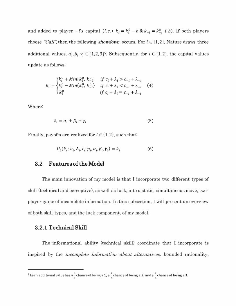
upper bound of 1. Finally, I have imposed the Expected Value constraint 4𝑦𝑖 − 𝑥𝑖 ≥ 1,

which is a structural assumption that assures that 𝐸[𝐿 3(𝑥𝑖 ,𝑦𝑖)] ≥ 𝐸[𝐿2(𝑥𝑖 ,𝑦𝑖)] ≥

𝐸[𝐿1(𝑥𝑖 ,𝑦𝑖)]. By applying this condition, and assuming the risk-neutrality of players,

I am able to create an ordinal ranking for each player’s preferences toward lottery-

types, such that 𝐿 3(𝑥𝑖 ,𝑦𝑖) ≿ 𝐿2(𝑥𝑖 ,𝑦𝑖) ≿ 𝐿 1(𝑥𝑖 ,𝑦𝑖). Upon considering each of the listed

constraints, the shaded region in Figure 2 shows the valid informational ability

coordinates for each player in my model.

Figure 2:

0

0.05

0.10.15

0.2

0.250.3

0.35

0.40.45

0.5

0.55

0.60.65

0.7

0.750.8

0.85

0.90.95

1

0

0.0

3

0.0

6

0.0

9

0.1

2

0.1

5

0.1

8

0.2

1

0.2

4

0.2

7

0.3

0.3

3

0.3

6

0.3

9

0.4

2

0.4

5

0.4

8

0.5

1

0.5

4

0.5

7

0.6

0.6

3

0.6

6

0.6

9

0.7

2

0.7

5

0.7

8

0.8

1

0.8

4

0.8

7

0.9

0.9

3

0.9

6

0.9

9

Y -

([1

] &

[3

] Lo

tter

y V

alu

es)

X - ([2] Lottery Value)

Range of Valid Informational Ability Coordinates

Expected Value Constraint Negativity Constraint

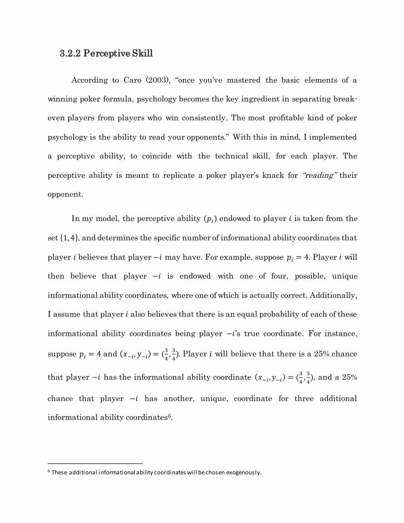
3.2.2 Perceptive Skill

According to Caro (2003), “once you’ve mastered the basic elements of a

winning poker formula, psychology becomes the key ingredient in separating break-

even players from players who win consistently. The most profitable kind of poker

psychology is the ability to read your opponents.” With this in mind, I implemented

a perceptive ability, to coincide with the technical skill, for each player. The

perceptive ability is meant to replicate a poker player’s knack for “reading” their

opponent.

In my model, the perceptive ability (𝑝𝑖) endowed to player 𝑖 is taken from the

set {1, 4}, and determines the specific number of informational ability coordinates that

player 𝑖 believes that player −𝑖 may have. For example, suppose 𝑝𝑖 = 4. Player 𝑖 will

then believe that player −𝑖 is endowed with one of four, possible, unique

informational ability coordinates, where one of which is actually correct. Additionally,

I assume that player 𝑖 also believes that there is an equal probability of each of these

informational ability coordinates being player −𝑖’s true coordinate. For instance,

suppose 𝑝𝑖 = 4 and (𝑥−𝑖 , 𝑦−𝑖) = (3

4,

3

4). Player 𝑖 will believe that there is a 25% chance

that player −𝑖 has the informational ability coordinate (𝑥−𝑖 ,𝑦−𝑖) = (3

4,

3

4), and a 25%

chance that player −𝑖 has another, unique, coordinate for three additional

informational ability coordinates6.

6 These additional informational ability coordinates will be chosen exogenously.

Upon considering the above example, it is clear that if 𝑝𝑖 = 1 then player 𝑖 has

perfect information regarding player −𝑖’s technical skill. Conversely, if 𝑝𝑖 = 4 then

player 𝑖 has imperfect information regarding player −𝑖’s technical skill. Finally, it is

important to note that, in my model, I am assuming that both players have perfect

information regarding the other player’s perceptive ability. That is, if 𝑝𝑖 = 𝑧; (𝑖 ∈ {1, 2}

and 𝑧 ∈ {1, 4}), then player −𝑖 knows that 𝑝𝑖 = 𝑧, and vice versa for player −𝑖.

3.2.3 Luck

The final feature of my model that I will discuss is the luck component that I

have incorporated. As quoted in Rodman et al. (2009), “to win tournaments, you’ve

got to play well and you’ve got to get lucky in some key spots”. Luck, in my model,

arises when both players specifically choose “Call”. When this happens, a showdown

occurs, and additional values, 𝛼𝑖 , 𝛽𝑖 and 𝛾𝑖 , are drawn for player 𝑖 (𝑖 ∈ {1,2}). Since

𝛼𝑖 , 𝛽𝑖 , and 𝛾𝑖 are drawn from the same distribution as player 𝑖’s hand-type, 𝑐𝑖, and

since all four parameters carry an equal weight when determining the updated

capital values, each player, in this case, will have made the decision to “Call” with

information that pertains to only one quarter of their total hand value (henceforth

referred to as a player’s score). So, regardless of what hand-type, 𝑐𝑖, players are dealt,

either player still has a chance to win. For instance, consider the case when player 𝑖

is dealt 𝑐𝑖 = 1, and player −𝑖 is dealt 𝑐−𝑖 = 3. If the additional values for player −𝑖 are

𝛼−𝑖 = 1, 𝛽−𝑖 = 1, and 𝛾−𝑖 = 1, then player −𝑖’s score would be 𝑐−𝑖 + 𝜆−𝑖 = 𝑐−𝑖 + 𝛼−𝑖 +

𝛽−𝑖 + 𝛾−𝑖 = 6. Now, since 𝑐𝑖 = 1, any combination of 𝛼𝑖, 𝛽𝑖, and 𝛾𝑖 such that 𝛼𝑖 + 𝛽𝑖 +

𝛾𝑖 ≥ 6 = 𝑐−𝑖 + 𝜆−𝑖 would lead to player 𝑖 winning the showdown over player −𝑖, despite

player 𝑖 drawing the lowest, initial, hand-type and player −𝑖 drawing the highest,

initial, hand-type. Appendix I lists the probabilities of a player winning, drawing, or

losing a showdown for every initial combination of hand-types.

4 Calibration

Prior to conducting a comparative static analysis on the model, I would first

like to calibrate some parameters to depict a benchmark case that replicates a

common situation for a poker hand. My reasoning for doing so will be outlined in the

following paragraphs. A summary of the benchmark structural parameters I utilize

is listed in Figure 3.

Figure 3: Structural parameters used in the Benchmark Case78

Parameter Value Interpretation

𝑘10 10 Player 1’s initial capital level

𝑘20 10 Player 2’s initial capital level

𝑏 1 The blind cost

(𝑥1,𝑦1) (1, 1) Player 1’s technical skill

(𝑥2,𝑦2 ) (1, 1) Player 2’s technical skill

𝑝1 1 Player 1’s perceptive skill

𝑝2 1 Player 2’s perceptive skill

At the beginning of any standard poker tournament, all players have the same

amount of capital. So, for the benchmark case, I chose to set the initial capital level

for player 1 equal to the initial capital level for player 2. In some tournaments,

however, players may start with varying levels of capital. Also, as a tournament

7 For the benchmark case, I have set (𝑥1 ,𝑦1

) = (𝑥2 ,𝑦2) = (1, 1) to give a baseline assumption that each player has

perfect technical skill . 8 For the benchmark case, I have set 𝑝1 = 𝑝2 = 1 to give a baseline assumption that each player has perfect

perceptive skil l.

progresses, players will very likely have disparate capital levels. Accordingly, I will

conduct analysis based on how player behaviour changes as I alter the capital-level

ratio between the two players. Nevertheless, for the benchmark case, I have assumed

capital-level symmetry between the two players.

Given that 𝑘10 = 𝑘2

0 = 𝑘0, an interesting property of the model is that the

absolute capital and blind levels do not, necessarily, matter for the purpose of

analysis. Instead, it is the relative values between these parameters that are

important. Since I have assumed risk-neutrality for both players, the payoffs for each

player will always be scaled by the same factor as that of which the structural

parameters are scaled by. For example, consider the case where I scale the

parameters by a factor of 𝑥. This will result with the parameters being 𝑘1∗ = 𝑘2

∗ = 𝑥𝑘0

and 𝑏∗ = 𝑥𝑏. The payoffs, for each player (𝑖 ∈ {1, 2}), will be as follows:

If both players were to “Fold”

𝑈𝑖( ∙ ) = 𝑘𝑖 = 𝑘𝑖∗ − 𝑏∗ + 𝑏∗ = 𝑥𝑘𝑖

0 (7)

If player 𝑖 were to “Call” and player −𝑖 were to “Fold”:

𝑈𝑖( ∙ ) = 𝑘𝑖 = 𝑘𝑖∗ + 𝑏∗ = 𝑥𝑘𝑖

0 + 𝑥𝑏 = 𝑥(𝑘𝑖0 + 𝑏) (8)

𝑈−𝑖( ∙ ) = 𝑘−𝑖 = 𝑘−𝑖∗ − 𝑏∗ = 𝑥𝑘−𝑖

0 − 𝑥𝑏 = 𝑥(𝑘−𝑖0 − 𝑏) (9)

If player 𝑖 were to “Fold” and player −𝑖 were to “Call”:

𝑈𝑖( ∙ ) = 𝑘𝑖 = 𝑘𝑖∗ − 𝑏∗ = 𝑥𝑘𝑖

0 − 𝑥𝑏 = 𝑥(𝑘𝑖0 − 𝑏) (10)

𝑈−𝑖( ∙ ) = 𝑘−𝑖 = 𝑘−𝑖∗ + 𝑏∗ = 𝑥𝑘−𝑖

0 + 𝑥𝑏 = 𝑥(𝑘−𝑖0 + 𝑏) (11)

If both players were to “Call”:

𝑈𝑖( ∙ ) = 𝑘𝑖

= {

𝑘𝑖∗ + 𝑀𝑖𝑛{𝑘𝑖

∗, 𝑘−𝑖∗ } = 𝑥(𝑘𝑖

0 + 𝑀𝑖𝑛{𝑘𝑖0, 𝑘−𝑖

0 }) 𝑖𝑓 𝑐𝑖 + 𝜆𝑖 > 𝑐−𝑖 + 𝜆−𝑖

𝑘𝑖∗ − 𝑀𝑖𝑛{𝑘𝑖

∗, 𝑘−𝑖∗ } = 𝑥(𝑘𝑖

0 − 𝑀𝑖𝑛{𝑘𝑖0, 𝑘−𝑖

0 }) 𝑖𝑓 𝑐𝑖 + 𝜆𝑖 < 𝑐−𝑖 + 𝜆−𝑖

𝑘𝑖∗ = 𝑥𝑘𝑖

0 𝑖𝑓 𝑐𝑖 + 𝜆𝑖 = 𝑐−𝑖 + 𝜆−𝑖

(12)

𝑈−𝑖( ∙ ) = 𝑘−𝑖

= {

𝑘−𝑖∗ + 𝑀𝑖𝑛{𝑘𝑖

∗, 𝑘−𝑖∗ } = 𝑥(𝑘−𝑖

0 + 𝑀𝑖𝑛{𝑘𝑖0, 𝑘−𝑖

0 }) 𝑖𝑓 𝑐−𝑖 + 𝜆−𝑖 > 𝑐𝑖 + 𝜆𝑖

𝑘−𝑖∗ − 𝑀𝑖𝑛{𝑘𝑖

∗, 𝑘−𝑖∗ } = 𝑥(𝑘−𝑖

0 − 𝑀𝑖𝑛{𝑘𝑖0, 𝑘−𝑖

0 }) 𝑖𝑓 𝑐−𝑖 + 𝜆−𝑖 < 𝑐𝑖 + 𝜆𝑖

𝑘−𝑖∗ = 𝑥𝑘−𝑖

0 𝑖𝑓 𝑐−𝑖 + 𝜆−𝑖 = 𝑐𝑖 + 𝜆𝑖

(13)

Therefore, based on the above results, if 𝑘10 = 𝑘2

0, then it is not the absolute values of

𝑘10, 𝑘2

0, and 𝑏 that matter for analysis, but instead it is the relative values of these

parameters that we should focus on.

A common inflection point for players in a poker tournament occurs when a

player’s capital level reaches a total of ten big blinds9. At this point, it is widely

known, amongst experienced players, that the benefits of aggressive play rise relative

to the benefits of passivity. Furthermore, at this stage, common advice to players is

to employ a strategic action set that consists of only two moves: raise all of your chips

or fold (Snyder, 2006). This advice was a contributing factor to my choice of utilizing

{𝐹𝑜𝑙𝑑, 𝐶𝑎𝑙𝑙} as the players’ action set; where, in my model, call is synonymous to raise

all of your chips. By setting 𝑘10 = 𝑘2

0 = 10 and 𝑏 = 1, I have effectively imposed, on

each player, a capital-to-blind ratio of 10-to-1, thereby making the action set

{𝐹𝑜𝑙𝑑, 𝐶𝑎𝑙𝑙} realistic. A noteworthy point to make is that Snyder (2006) advises

players with more than ten big blinds to also consider the action of raising to a value

that is less than all of your chips. In the Analysis section, I will alter the capital-to-

blind ratio of each player to determine optimal player behaviour when this ratio

exceeds 10-to-1 and when it is strictly less than 10-to-1.

9 Please see “Texas Hold’em Rules” (2016) for an explanation of what a big blind is specifically.

For convenience, I limited the set of possible informational ability coordinates,

for each player, to four. A summary of these four coordinates is listed in Figure 4. My

methodology for choosing the four coordinates is simple. First, I restricted the set of

possible coordinates to values of 𝑥𝑖 and 𝑦𝑖 (𝑖 ∈ {1,2}) that satisfy the Boundary,

Negativity, and Expected Value constraints, and are such that 𝑥𝑖 = 𝑦𝑖. Next, I

identified the coordinate that corresponds to perfect informational ability10, (𝑥𝑖 ,𝑦𝑖) =

(1,1), and the coordinate that corresponds to completely imperfect informational

ability11, (𝑥𝑖 ,𝑦𝑖) = (13⁄ , 1

3⁄ ). I, then, computed the expected values for each lottery-

type, for the perfect informational ability and completely imperfect informational

ability cases. Next, I took the difference between the expected value of 𝐿 3(1,1) and the

expected value of 𝐿1(1,1). I found this difference to equal 2. I repeated this for the

completely imperfect informational ability case, and found this expected value

difference to equal 0. Using these two extremes, I partitioned the range of expected

value differences into three equivalent regions, which provided me with two more

expected value differences to target, 23⁄ and 4

3⁄ . Finally, I solved for the

informational ability coordinates, (59⁄ , 5

9⁄ ) and (79⁄ , 7

9⁄ ), which respectively yielded

the two desired expected value differences. I subsequently used these two coordinates

as the middling, possible, informational ability coordinates for each player.

10 When a player has perfect informational ability, they are able to completely discern their hand type based on the specific lottery-type they draw. See Appendix A2 for the corresponding convex combination coefficients matrix for the case where (𝑥 𝑖 ,𝑦𝑖

) = (1,1). 11 When a player has completely imperfect informational ability, they are unable to attain, from the lottery-type they draw, any additional knowledge regarding their hand-type. See Appendix A2 for the corresponding convex

combination coefficients matrix for the case where (𝑥 𝑖 ,𝑦𝑖) = (1

3⁄ , 13⁄ ).

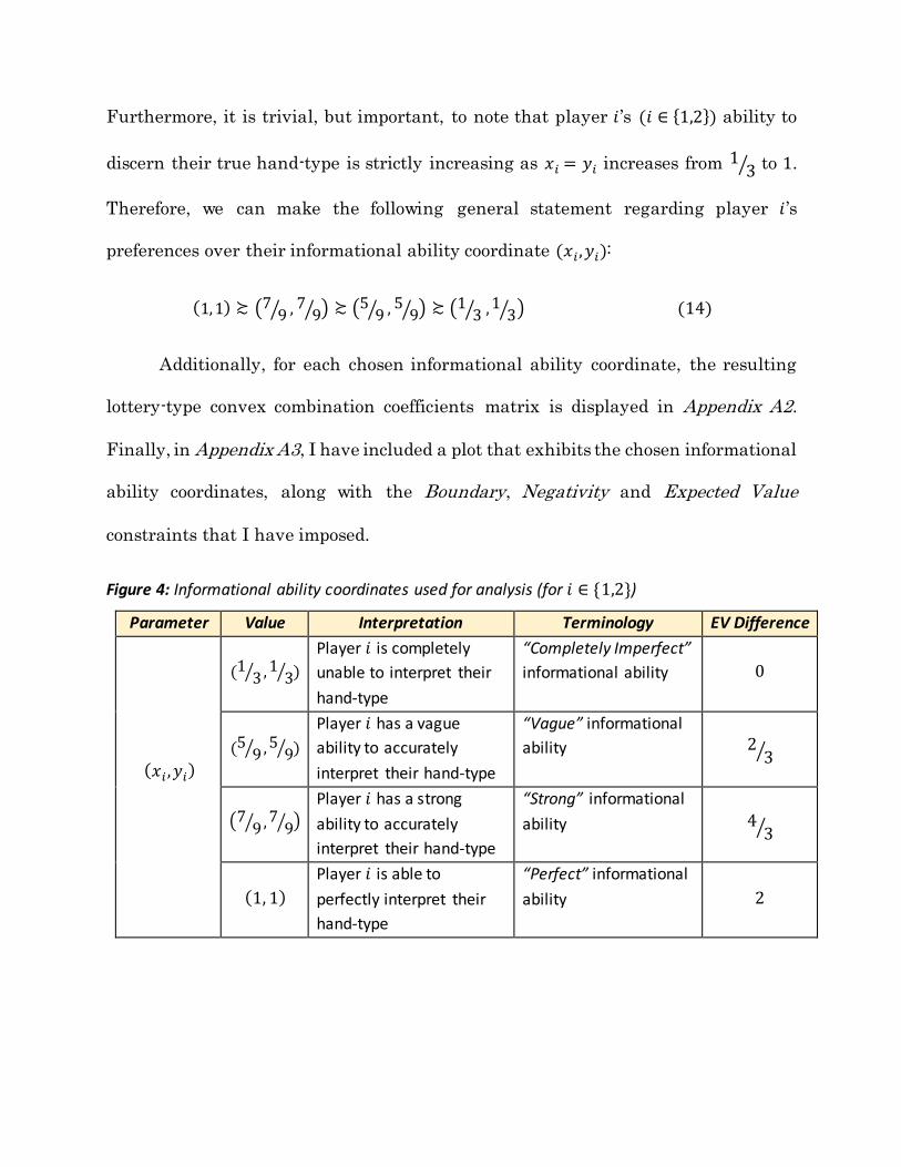
Furthermore, it is trivial, but important, to note that player 𝑖’s (𝑖 ∈ {1,2}) ability to

discern their true hand-type is strictly increasing as 𝑥𝑖 = 𝑦𝑖 increases from 13⁄ to 1.

Therefore, we can make the following general statement regarding player 𝑖’s

preferences over their informational ability coordinate (𝑥𝑖 ,𝑦𝑖):

(1, 1) ≿ (79⁄ , 7

9⁄ ) ≿ (59⁄ , 5

9⁄ ) ≿ (13⁄ , 1

3⁄ ) (14)

Additionally, for each chosen informational ability coordinate, the resulting

lottery-type convex combination coefficients matrix is displayed in Appendix A2.

Finally, in Appendix A3, I have included a plot that exhibits the chosen informational

ability coordinates, along with the Boundary, Negativity and Expected Value

constraints that I have imposed.

Figure 4: Informational ability coordinates used for analysis (for 𝑖 ∈ {1,2})

Parameter Value Interpretation Terminology EV Difference

(𝑥𝑖 ,𝑦𝑖)

(13⁄ , 1

3⁄ )

Player 𝑖 is completely

unable to interpret their

hand-type

“Completely Imperfect”

informational ability

0

(59⁄ , 5

9⁄ )

Player 𝑖 has a vague

ability to accurately

interpret their hand-type

“Vague” informational

ability

2

3⁄

(79⁄ , 7

9⁄ )

Player 𝑖 has a strong

ability to accurately

interpret their hand-type

“Strong” informational

ability

4

3⁄

(1, 1)

Player 𝑖 is able to

perfectly interpret their

hand-type

“Perfect” informational

ability

2

5 Analysis

In this section, I will present a comparative static analysis based on altering

the parameters of my model from the parameters I outlined for the benchmark case.

A summary of the cases presented in this section is listed in Appendix A4. Before

proceeding, I would like to detail some preliminary insights that we should consider

throughout our analysis.

5.1 Preliminaries

The solution concept I use is that of a Bayesian-Nash equilibrium12. Recall that

a Bayesian-Nash equilibrium, for a two-player game, is a strategy profile and belief

specification, for each player regarding the types of the other player, that maximizes

the expected payoff for each player given their beliefs about the other player’s type(s)

and given the other player’s strategy. Also, recall that a strategy for a Bayesian game

is a complete, contingent plan that specifies a player’s action for every type that

player may be. Now, relating this to my model, notice that player 𝑖’s (𝑖 ∈ {1, 2})

strategy (𝑠𝑖) will be a vector consisting of the following three parameters:

𝑎𝑖(𝐿1(𝑥𝑖 ,𝑦𝑖)), 𝑎𝑖(𝐿2(𝑥𝑖 ,𝑦𝑖)), and 𝑎𝑖(𝐿3(𝑥𝑖 ,𝑦𝑖)). The notation I use to denote player 𝑖’s

strategy is:

𝑠𝑖 = (𝑎𝑖(𝐿1(𝑥𝑖 ,𝑦𝑖)),𝑎𝑖(𝐿 2(𝑥𝑖 ,𝑦𝑖)),𝑎𝑖(𝐿3(𝑥𝑖 ,𝑦𝑖))) (15)

12 The format I use to display the Bayesian-Nash equilibrium is {𝑠1 , 𝑠2}, where 𝑠𝑖 (𝑖 ∈ {1,2}) represents the Bayesian-

Nash equilibrium strategy vector for player 𝑖.

The reason that player 𝑖’s strategy only contains three parameters, despite the many

types that player 𝑖 may be, is that many of the types, specifically player 𝑖’s

informational ability and perceptive ability, will be predefined for each case that I

conduct. Furthermore, notice that I have also not included player 𝑖’s hand-type in

their strategy vector. My reason for this is that player 𝑖’s hand-type is essentially

drawn after player 𝑖 has already chosen their strategy. Player 𝑖’s specific hand-type

only becomes a factor when computing player 𝑖’s score in a showdown, whereas player

𝑖’s strategy is selected based on an expectation of the hand-type they will draw.

Additionally, since both players are risk-neutral and receive payoffs equal to

their post-game capital level, each case I analyze will be a zero-sum game. Therefore,

the sum of the payoffs the players receive will always equal the sum of the players’

initial capital levels.

Finally, I would like to summarize the beliefs that player 𝑖 (𝑖 ∈ {1, 2}) has in

the game I outlined above, given player −𝑖’s perceptive ability, 𝑝−𝑖, as well as both

players’ informational ability, (𝑥𝑖 ,𝑦𝑖) and (𝑥−𝑖 ,𝑦−𝑖). First, player 𝑖 believes that, given

the lottery-type, 𝐿𝑗(𝑥𝑖 ,𝑦𝑖) (𝑗 ∈ {1, 2, 3}), the probability that player 𝑖 has of drawing a

specific hand-type, 𝑐𝑖, is equal to the corresponding value of the convex combination

coefficients matrix shown in Figure 1 (on page 11). Second, player 𝑖 believes that

player −𝑖 has a 1

3 probability of drawing each specific hand-type, 𝑐−𝑖, and each specific

lottery-type, 𝐿𝑗(𝑥−𝑖 ,𝑦−𝑖). Third, if 𝑝𝑖 = 1, then player 𝑖 believes for certain that player

−𝑖 has the informational ability, (𝑥−𝑖 , 𝑦−𝑖). Fourth, if 𝑝𝑖 = 4, then player 𝑖 believes that

there is a 1

4 probability that player −𝑖 has the informational ability, (𝑥−𝑖 , 𝑦−𝑖), as well

as a 1

4 probability that player −𝑖 has each of the remaining, possible, informational

abilities (�̇�−𝑖 , �̇�−𝑖), (�̈�−𝑖 , �̈�−𝑖), and (𝑥−𝑖 , 𝑦−𝑖)13. Finally, player 𝑖 believes for certain that

player −𝑖 has the perceptive ability, 𝑝−𝑖.

5.2 Case Analysis

In this subsection, I will conduct a case-by-case comparative static analysis on

my model. I will begin each case by presenting an overview of the structural

parameters I used and the results I obtained for that specific case. I will follow each

case with a brief discussion detailing the corresponding results. Although most of the

results are easy to interpret, it is essential for me to elaborate on the difference

between player 𝑖’s (𝑖 ∈ {1, 2}) expected payoff and player 𝑖’s actual payoff. Player 𝑖’s

expected payoff is the payoff that player 𝑖 expects to attain after considering all of

their beliefs and choosing an action, but before player −𝑖’s perceptive ability is

revealed to them. Player 𝑖’s actual payoff is the payoff that player 𝑖 would expect to

receive after considering all of their beliefs, choosing an action, and observing player

−𝑖’s perceptive ability.

13 That is, if 𝑝𝑖 = 4, then player 𝑖 believes that there is a

1

4 probability that player −𝑖 has each of the following

informational abilities: (1,1), (79⁄ , 7

9⁄ ), (59⁄ , 5

9⁄ ), (13⁄ , 1

3⁄ ).

5.2.1 Benchmark Case

Figure 5: Structural parameters & results for the Benchmark Case

Sub-case

Player Blind Cost

Initial Capital

Technical Skill

Perceptive Skill14

Bayesian-Nash

Equilibria

Expected Payoff

Actual Payoff

BM 1

1 10 Perfect Perfect (F,F,C) 10 10


The benchmark case is quite straightforward, with only a few noteworthy

results. The first is that, since this game is symmetric, the actual payoffs for each

player, 𝑖 (𝑖 ∈ {1,2}), will be equivalent to that of the other player, −𝑖. Furthermore,

this implies that, since this is a two-player, zero-sum game, the actual payoffs for

each player will equal the players’ initial capital level. Additionally, since both

players have perfect perceptive skill and the same level of technical skill, neither

player will expect to have an advantage over their opponent, thereby resulting in the

players’ expected payoffs to be equal to the players’ initial capital level.

Finally, notice that the Bayesian-Nash equilibrium for this case is

{(𝐹, 𝐹, 𝐶),(𝐹, 𝐹, 𝐶)}. Therefore, in this equilibrium, both players will be playing a

conservative, yet selectively aggressive strategy where each player will call with

𝐿 3(1,1), but fold with 𝐿 2(1,1) and 𝐿1(1,1). This will be important to consider when

comparing the Bayesian-Nash equilibria that arise from the other cases I study.

14 Under Perceptive Skill, “Perfect” corresponds to a player, 𝑖 (𝑖 ∈ {1,2}), such that 𝑝𝑖 = 1; “Imperfect” corresponds

to a player, 𝑖 (𝑖 ∈ {1,2}), such that 𝑝𝑖 = 4.

5.2.2 Altering the Blind Cost

Figure 6: Results obtained when altering the blind cost (𝑏):

Sub-case:

Player Blind Cost

Initial Capital

Technical Skill

Perceptive Skill

Bayesian-Nash

Equilibria

Expected Payoff

Actual Payoff

1 1

0 10 Perfect Perfect

Multiple15 10 10

2 10 Perfect Perfect 10 10

2 1

0.01 10 Perfect Perfect (F,F,C) 10 10


3 1

0.5 10 Perfect Perfect (F,F,C) 10 10


4 (BM)

1 1

10 Perfect Perfect (F,F,C) 10 10


5 1 889

729⁄ 10 Perfect Perfect (F,F,C) 10 10


6 1 890

729⁄ 10 Perfect Perfect

Multiple16 10 10


7 1 891

729⁄ 10 Perfect Perfect (F,C,C) 10 10

2 10 Perfect Perfect (F,C,C) 10 10

8 1



9 1



10 1

4 10 Perfect Perfect (C,C,C) 10 10


11 1



For this study, I held each of the structural parameters, except for the blind

cost (𝑏), consistent to that of the benchmark case. By altering the value of the blind

15 The following four Bayesian-Nash equilibria were found for this case: {(𝐹, 𝐹, 𝐹), (𝐹, 𝐹, 𝐹)}, {(𝐹 , 𝐹, 𝐹), (𝐹 ,𝐹, 𝐶)}, {(𝐹, 𝐹, 𝐶), (𝐹, 𝐹, 𝐹)}, and {(𝐹, 𝐹, 𝐶), (𝐹, 𝐹, 𝐶)}. Each equilibrium resulted in both players receivi ng an expected

payoff of 10 and an actual payoff of 10. 16 The following three Bayesian-Nash equilibria were found for this case: {(𝐹, 𝐹, 𝐶), (𝐹, 𝐹, 𝐶)}, {(𝐹 , 𝐹, 𝐶), (𝐹, 𝐶, 𝐶)},

and {(𝐹, 𝐶, 𝐶), (𝐹, 𝐹, 𝐶)}. Each equilibrium resulted in both players receivi ng an expected payoff of 10 and an actual

payoff of 10.

cost, I am essentially changing the expense of folding as well as the additional payoff

a player would receive by calling when their opponent folds.

First, for the same reasons outlined in the benchmark case, the expected and

actual payoffs for each player, in this situation, will equal the players’ initial capital

level. Second, an interesting characteristic of this case is that as the blind cost

increases, the players’ Bayesian-Nash equilibria strategies become more aggressive.

This result is intuitive because as the blind cost increases, both the price of folding

and the potential reward for calling increases, which thereby magnifies the benefits

of aggressive play. This result is also consistent with common poker insight that

advises poker players to play more aggressively as the blinds increase.

Finally, it is interesting to note the subcases where multiple Bayesian-Nash

equilibria exist. The blind costs for these cases are threshold points where the

equilibrium strategies switch from a more conservative strategy to a more aggressive

strategy. Subcase 1 is particularly interesting because of the existence of Bayesian-

Nash equilibrium strategies that have players of perfect technical skill folding the

highest lottery-type, which is, essentially, the best possible hand-type since both

players have perfect informational ability. However, this is not difficult to reconcile

since a blind cost of zero implies that the players will not incur a cost of folding, and

since both players know that the other player is of the same technical ability, neither

will have an advantage of playing, which therefore makes folding all hands a viable

strategy.

5.2.3 Altering the Players’ Initial Capital Ratio

Figure 7: Results obtained when altering the players’ initial capital ratio (𝑘10

𝑘20⁄ ):

Sub-case

Player Blind Cost

Initial Capital

Technical Skill

Perceptive Skill

Bayesian-Nash

Equilibria

Expected Payoff

Actual Payoff

1 1



2 1



3 1

1 2.915 Perfect Perfect (C,C,C) 2.915 2.915


4 1

1 2.916 Perfect Perfect

Multiple17 2.916 2.916


5 1

1 2.917 Perfect Perfect (F,C,C) 2.917 2.917


6 1



7 1

1 8.19 Perfect Perfect (F,C,C) 8.19 8.19


8 1

1 7290

890⁄ Perfect Perfect Multiple18

7290890⁄ 7290

890⁄


9 1

1 8.2 Perfect Perfect (F,F,C) 8.2 8.2


10 (BM)

1 1



11 1



17 The following four Bayesian-Nash equilibria were found for this case: {(𝐹 , 𝐶, 𝐶), (𝐹, 𝐶, 𝐶)}, {(𝐹, 𝐶, 𝐶), (𝐶, 𝐶, 𝐶)}, {(𝐶, 𝐶, 𝐶), (𝐹, 𝐶, 𝐶)}, and {(𝐶, 𝐶, 𝐶), (𝐶, 𝐶, 𝐶)}. Each equilibrium resulted in players 1 and 2 receiving expected payoffs of 2.916 and 10 respectively, and actual payoffs of 2.916 and 10 respectively. 18 The following three Bayesian-Nash equilibria were found for this case: {(𝐹, 𝐹, 𝐶), (𝐹, 𝐹, 𝐶)}, {(𝐹 , 𝐹, 𝐶), (𝐹, 𝐶, 𝐶)},

and {(𝐹, 𝐶, 𝐶), (𝐹, 𝐹, 𝐶)}. Each equilibrium resulted in players 1 and 2 receiving expected payoffs of 7290890⁄ and

10 respectively, and actual payoffs of 7290890⁄ and 10 respectively.

For this case, I held the structural parameters consistent to that of the

benchmark case, except, this time, I altered the players’ initial capital ratio, (𝑘10

𝑘20⁄ ).

By changing this ratio, I effectively made one player, initially, richer in capital than

the other.

For similar reasons as in the previous cases, the expected and actual payoffs

for each player will equal the players’ initial capital level. Also, notice that as I

increase the players’ initial capital ratio, the Bayesian-Nash equilibrium strategies

for both players become more conservative. It makes sense that player 1 would want

to play an aggressive strategy since the blind cost is proportionally higher to their

initial capital level when their initial capital level is low. It’s somewhat unintuitive

as to why player 2’s equilibrium strategy always seems to mirror player 1’s

equilibrium strategy. However, the reason for this is that when 𝑘20 > 𝑘1

0, player 2 can

only lose a maximum of 𝑘10, and since both players are risk-neutral, each player will

value the risk equal to that of the other player. This, thereby, induces strategic

symmetry between player 1 and player 2, despite their different initial capital levels.

Furthermore, for this case, when 𝑘𝑖0 > 𝑘−𝑖

0 (𝑖 ∈ {1,2}), the game presented is

equivalent to that of where 𝑘𝑖0 = 𝑘−𝑖

0 , and player 𝑖 has 𝑘𝑖0 − 𝑘−𝑖

0 added to their post-

game capital level. Now, recall our conjecture in the Calibration section, such that it

is not the absolute values of 𝑘𝑖0, 𝑘−𝑖

0 , and 𝑏 that matter for analysis, but instead it is

the relative values of these parameters that are important. With this in mind, the

deterministic parameters in this case are �̂� = 𝑀𝑖𝑛{𝑘10, 𝑘2

0} and 𝑏, which effectively

makes it identical to the case where I only altered the blind cost. This can be verified

by comparing the subcases, for each case, that have identical �̂�-to-𝑏 ratios19.

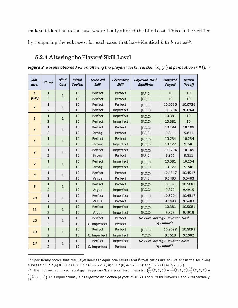
5.2.4 Altering the Players’ Skill Level

Figure 8: Results obtained when altering the players’ technical skill (𝑥𝑖 ,𝑦𝑖) & perceptive skill (𝑝𝑖):

Sub- case:

Player Blind Cost

Initial Capital

Technical Skill

Perceptive Skill

Bayesian-Nash Equilibria

Expected Payoff

Actual Payoff

1 (BM)

1 1



2 1

1 10 Perfect Perfect (F,F,C) 10.0736 10.0736

2 10 Perfect Imperfect (F,C,C) 10.3204 9.9264

3 1

1 10 Perfect Imperfect (F,C,C) 10.381 10

2 10 Perfect Imperfect (F,C,C) 10.381 10

4 1

1 10 Perfect Perfect (F,C,C) 10.189 10.189

2 10 Strong Perfect (F,F,C) 9.811 9.811

5 1


2 10 Strong Imperfect (F,C,C) 10.127 9.746

6 1


2 10 Strong Perfect (F,F,C) 9.811 9.811

7 1



8 1


2 10 Vague Perfect (F,F,C) 9.5483 9.5483

9 1


2 10 Vague Imperfect (F,C,C) 9.873 9.4919

10 1


2 10 Vague Perfect (F,F,C) 9.5483 9.5483

11 1



12 1

1 10 Perfect Perfect No Pure Strategy Bayesian-Nash

Equilibria20 2 10 C. Imperfect Perfect

13 1


2 10 C. Imperfect Imperfect (C,C,C) 9.7618 9.1902

14 1

1 10 Perfect Imperfect No Pure Strategy Bayesian-Nash

Equilibria20 2 10 C. Imperfect Perfect

19 Specifically notice that the Bayesian-Nash equilibria results and 𝑘-to-𝑏 ratios are equivalent in the following

subcases: 5.2.2 (4) & 5.2.3 (10); 5.2.2 (6) & 5.2.3 (8); 5.2.2 (8) & 5.2.3 (6); and 5.2.2 (11) & 5.2.3 (2). 20 The following mixed strategy Bayesian-Nash equilibrium exists: {

50

57(𝐹, 𝐶, 𝐶) +

7

57(𝐶, 𝐶, 𝐶),

27

38(𝐹, 𝐹, 𝐹) +

11

38(𝐶, 𝐶, 𝐶)}. This equilibrium yields expected and actual payoffs of 10.71 and 9.29 for Player’s 1 and 2 respectively.

15 1



16 1

1 10 Strong Perfect (F,C,C) 10 10


17 1


2 10 Strong Imperfect (F,C,C) 10.127 10

18 1



19 1

1 10 Strong Perfect (F,C,C) 10.254 10.254

2 10 Vague Perfect (F,C,C) 9.746 9.746

20 1



21 1



22 1



23 1


2 10 C. Imperfect Perfect (C,C,C) 9.5713 9.5713

24 1



25 1



26 1



27 1

1 10 Vague Perfect (F,C,C) 10 10


28 1


2 10 Vague Imperfect (F,C,C) 9.873 10

29 1



30 1



31 1



32 1



33 1



34 1

1 10 C. Imperfect Perfect (C,C,C) 10 10


35 1


2 10 C. Imperfect Imperfect (C,C,C) 10 10

36 1



For this study, I held the blind cost and initial capital levels consistent to that

of the benchmark case, while testing every combination of technical and perceptive

skill between the players.

For subcases 2, 5, 6, 9, 13, 17, 20, and 24, when one player has perfect

perceptive skill while the other player does not, the player that does not begins the

game expecting to receive a certain payoff, but will actually yield a lesser payoff.

Whereas, the player with perfect perceptive ability will yield an equivalent payoff to

that which they expect. Subcase 2 is particularly interesting. Here, both players have

perfect technical skill, however, player 1 has perfect perceptive ability while player 2

has imperfect perceptive ability. Notice that if both players were able to discern the

other player’s technical ability, the Bayesian-Nash equilibrium would be

{(𝐹, 𝐹, 𝐶),(𝐹, 𝐹, 𝐶)}. Yet, since player 2 is unable to discern player 1’s technical skill,

the Bayesian-Nash equilibrium is, instead, {(𝐹, 𝐹, 𝐶),(𝐹, 𝐶, 𝐶)}. Therefore, in this

subcase, player 2 will be playing a non-optimal, more aggressive strategy than she

would have played if she had perfect perceptive ability. In addition to this, given each

player’s knowledge of their own perfect technical skill, both players expect to receive

a higher payoff than their initial capital level. Player 1, due to their perfect perceptive

ability, will accurately gauge their payoff, whereas player 2 will drastically

overestimate their payoff. The underlying reason behind player 2’s overestimation is

that player 2 believes that there is an equal probability of player 1 having a perfect,

strong, vague, or completely imperfect technical skill. Unfortunately for player 2,

player 1 has perfect technical skill, and is thereby able to capitalize on player 2’s

inability to discern player 1’s technical skill.

Now, consider subcase 10. The only structural difference between this subcase

and that of subcase 2 is that the player with perfect perceptive ability now has vague

technical skill. What’s interesting here is that player 1, who has perfect technical skill

but imperfect perceptive skill, expects the same payoff as they did in subcase 2.

However, this time, the payoff they actually receive will be higher than expected, for

a reason similar to that that was elaborated in the previous paragraph.

Another interesting result is that without the presence of a player with perfect

technical skill, altering the players’ perceptive ability, while holding all other

structural parameters constant, does not affect the Bayesian-Nash equilibria nor

does it affect the actual payoffs the players receive21. Therefore, for my case study,

the absence of a player with perfect technical skill implies that the perceptive abilities

only affect the payoff expectations that players may have. Additionally, there is no

case in which changing a player’s perceptive ability from perfect to imperfect, while

holding all else constant, benefits the player in terms of their actual payoff. However,

consider subcases 4 and 7. Here, it is interesting to note that if we take players with

perfect and strong technical skill respectively, and switch both of their perceptive

abilities from perfect to imperfect, the player with perfect technical skill will receive

21 This is true for the specific blind cost, initial capital levels, and technical skill possibilities that I have allowed for in this case. For example, changing the players’ perceptive abilities could also lead to different Bayesian-Nash equilibria outcomes and actual payoffs of the game in the absence of a player with perfect technical skill, (𝑥 𝑖 ,𝑦𝑖

) = (1, 1), but

in the presence of a player with almost perfect technical skil l (𝑖. 𝑒. (𝑥 𝑖 ,𝑦𝑖) = (0.99, 0.99)).

a higher actual payoff than before, whereas the player with strong technical skill will

receive a lower actual payoff than before. This also holds true if the player with strong

technical skill instead has vague or completely imperfect technical ability.

Next, notice that the Bayesian-Nash equilibria generated in this case indicate

that players with a high technical skill tend to play selectively aggressive strategies,

such as (𝐹, 𝐹, 𝐶) and (𝐹, 𝐶, 𝐶), in order to capitalize on the mistakes of lesser skilled

players22. Consider a player that has perfect technical skill. This player is able to

select a level of aggression that maximizes their payoff according to the technical skill

of their opponent. As shown in subcases 1, 4, 8, and 12, the perfectly skilled player is

able to adjust their level of aggression as the technical skill of their opponent

decreases. Furthermore, players with completely imperfect technical skill tend to

play recklessly aggressive strategies, such as (𝐶, 𝐶, 𝐶). This allows players with a high

technical skill to adjust their level of aggression in order to maximize their payoff.

These observations align with those stated by Rodman et al. (2009) and Siler (2010),

along with conventional poker wisdom that emphasizes the importance of adjusting

your strategy based on your opponents’ strategy.

Finally, to conclude the analysis, I will state some general observations that

we can learn from the results listed in Figure 8. Based on these subcases, it seems

that, in general, a player’s technical ability is the primary determinant of that

22 There are two types of mistakes that players can make in my model. These mistakes are:

I) Mistaking a poor hand for a good hand by drawing a high lottery-type and a low hand-type (for

example: A strong player that draws 𝐿3(79⁄ , 7

9⁄ ) and decides to call, but is actually dealt 𝑐𝑖 = 1).

II) Mistaking a good hand for a poor hand by drawing a low lottery-type and a high hand-type (for

example: A strong player that draws 𝐿1(79⁄ , 7

9⁄ ) and decides to fold, but is actually dealt 𝑐𝑖 = 3).

player’s payoff, whereas a player’s perceptive ability only serves to directly benefit

players of a high technical skill. While, for all other technical skill-types, a player’s

perceptive ability merely affects that player’s ability to gauge their actual payoff.

Also, subcase 2 generates an interesting result in the sense that the overconfidence

of a player with perfect technical skill and imperfect perceptive ability may get that

player into trouble when they enter the game expecting to win capital, but instead,

lose capital. This occurrence is similar to a realistic situation where a highly-skilled

online poker professional enters a poker game against a live-play poker professional.

Online poker players are known to have great technical ability, but sometimes lack

the perceptive skill that live players possess. In this case, the lack of perceptive skill

would lead to the live-play professional having an advantage over the online

professional. Furthermore, we should not discount the importance of a player’s

perceptive ability entirely. Notice that the perceptive skill is particularly important

when highly skilled players are present, which is true for most major poker

tournaments. This aligns with Caro’s (2003) claim that “once you’ve mastered the

basic elements of a winning poker formula, psychology becomes the key ingredient in

separating break-even players from players who win consistently. The most

profitable kind of poker psychology is the ability to read your opponents.”

6 Conclusion

The purpose of this paper was to present an original model, motivated by the

first betting round in a single, two-player, hand of No-Limit Hold’em poker. The

model I exhibit features two, risk-neutral, players engaging in a static, simultaneous-

move game of incomplete information, and incorporates luck as well as two different

types of skill, technical and perceptive. Through a comparative static analysis that

altered the structural parameters of my model, I developed insight regarding the

parametric effects of the model. Furthermore, the insights that I produce align with

conventional poker wisdom, as well as the results obtained by other works of

literature.

This paper is just the preliminary step of my research using this model, as

there are various extensions that I would like to make. First, I would like to link the

insights I obtained to online poker data. I plan to do this by using hand histories

compiled by HHSmithy.com, an online datamining service that tracks thousands of

online poker hands daily. Second, I would like to draw parallels between my model

and other strategic interactions in economics and industrial organization, then use

my model to develop insights on these other areas. Finally, I would like to incorporate

an experimental component that features subjects playing the game I outlined above.

It would be interesting to observe how experimental subjects approach my game, and

to see if the subjects act differently than my model predicts.

7 References

Alaoui, L., & Fons-Rosen, C. (2016). Know when to fold'em: The grit factor.

Ando, M. (2004). Overconfidence in economic contests. Available at SSRN 539902.

Aumann, R. J., & Heifetz, A. (2002). Incomplete information. Handbook of game theory with economic applications, 3, 1665-1686.

Billings, D., Davidson, A., Schaeffer, J., & Szafron, D. (2002). The challenge of poker. Artificial Intelligence, 134(1), 201-240.

Billings, D., Burch, N., Davidson, A., Holte, R., Schaeffer, J., Schauenberg, T., &

Szafron, D. (2003, August). Approximating game-theoretic optimal strategies for full-scale poker. In IJCAI (pp. 661-668).

Borm, P., & Van Der Genugten, B. (2000). On the exploitation of casino games: How

to distinguish between games of chance and games of skill?. In Game Practice: Contributions from Applied Game Theory (pp. 19-33). Springer US.

Borm, P., & van der Genugten, B. (2001). On a relative measure of skill for games with chance elements. Top, 9(1), 91-114.

Burns, K. (2004). Heads-up face-off: On style and skill in the game of poker. In Style

and Meaning in Language, Art, Music, and Design: Papers from the 2004 Fall Symposium (pp. 15-22).

Caro, M. (2003). Caro's book of poker tells. Cardoza Publishing. (pp. 8)

Croson, R., Fishman, P., & Pope, D. G. (2008). Poker superstars: skill or luck?

Similarities between golf—thought to be a game of skill—and poker. Chance, 21(4), 25–28.

Dreef, M., Borm, P., & Genugten, B. V. D. (2004). Measuring skill in games: Several

approaches discussed. Mathematical methods of operations Research, 59(3), 375-391.

Griffiths, M., Parke, J., Wood, R., & Rigbye, J. (2010). Online poker gambling in

university students: Further findings from an online survey. International Journal of Mental Health and Addiction, 8(1), 82-89.

Haltiwanger, J., & Waldman, M. (1985). Rational expectations and the limits of

rationality: An analysis of heterogeneity. The American Economic Review, 75(3), 326-340.

Hannum, R. C., & Cabot, A. N. (2009). Toward legalization of poker: The skill vs. chance debate. UNLV Gaming Research & Review Journal, 13(1), 1.

Holden, A. (2008). Bigger deal: A year inside the poker boom. Simon and Schuster, 8–9.

Jehiel, P., & Koessler, F. (2008). Revisiting games of incomplete information with analogy-based expectations. Games and Economic Behavior, 62(2), 533-557.

Korb, K. B., Nicholson, A. E., & Jitnah, N. (1999, July). Bayesian poker. In

Proceedings of the Fifteenth conference on Uncertainty in artificial intelligence (pp.

343-350). Morgan Kaufmann Publishers Inc..

Levitt, S. D., & Miles, T. J. (2014). The role of skill versus luck in poker evidence from the world series of poker. Journal of Sports Economics, 15(1), 31-44.

Ludwig, S., Wichardt, P. C., & Wickhorst, H. (2011). Overconfidence can improve an

agent's relative and absolute performance in contests. Economics Letters, 110(3), 193-196.

McCormack, A., & Griffiths, M. D. (2012). What differentiates professional poker

players from recreational poker players? A qualitative interview study. International Journal of Mental Health and Addiction, 10(2), 243-257.

Meyer, G., von Meduna, M., Brosowski, T., & Hayer, T. (2013). Is poker a game of

skill or chance? A quasi-experimental study. Journal of Gambling Studies, 29(3), 535-550.

Texas Hold’em Rules. (2016, September 23). Retrieved from https://www.pokerschoolonline.com/articles/Texas-Hold-em-Rules

Rapoport, A., Erev, I., Abraham, E. V., & Olson, D. E. (1997). Randomization and

adaptive learning in a simplified poker game. Organizational Behavior and Human Decision Processes, 69(1), 31-49.

Rodman, B., Nelson, L., Heston, S., & Hellmuth Jr, P. (2009). Kill Phil: The Fast Track to Success in No-limit Hold'em Poker Tournaments. Huntington Press Inc.

(pp. 193)

Shi, J., & Littman, M. L. (2000, October). Abstraction methods for game theoretic

poker. In International Conference on Computers and Games (pp. 333-345). Springer Berlin Heidelberg.

Siler, K. (2010). Social and psychological challenges of poker. Journal of Gambling Studies, 26(3), 401-420.

Simon, H. A. (1972). Theories of bounded rationality. Decision and organization, 1(1), 161-176.

Snyder, A. (2006). The Poker Tournament Formula. Cardoza Publishing. (pp. 117-

127)

Southey, F., Bowling, M. P., Larson, B., Piccione, C., Burch, N., Billings, D., &

Rayner, C. (2012). Bayes' bluff: Opponent modelling in poker. arXiv preprint arXiv:1207.1411.

https://www.pokerschoolonline.com/articles/Texas-Hold-em-Rules

WSOP.com. (2016, September 19). Retrieved from http://www.wsop.com/tournaments/results.asp?rr=5&grid=1232&tid=14968&dayof=

8 Appendices

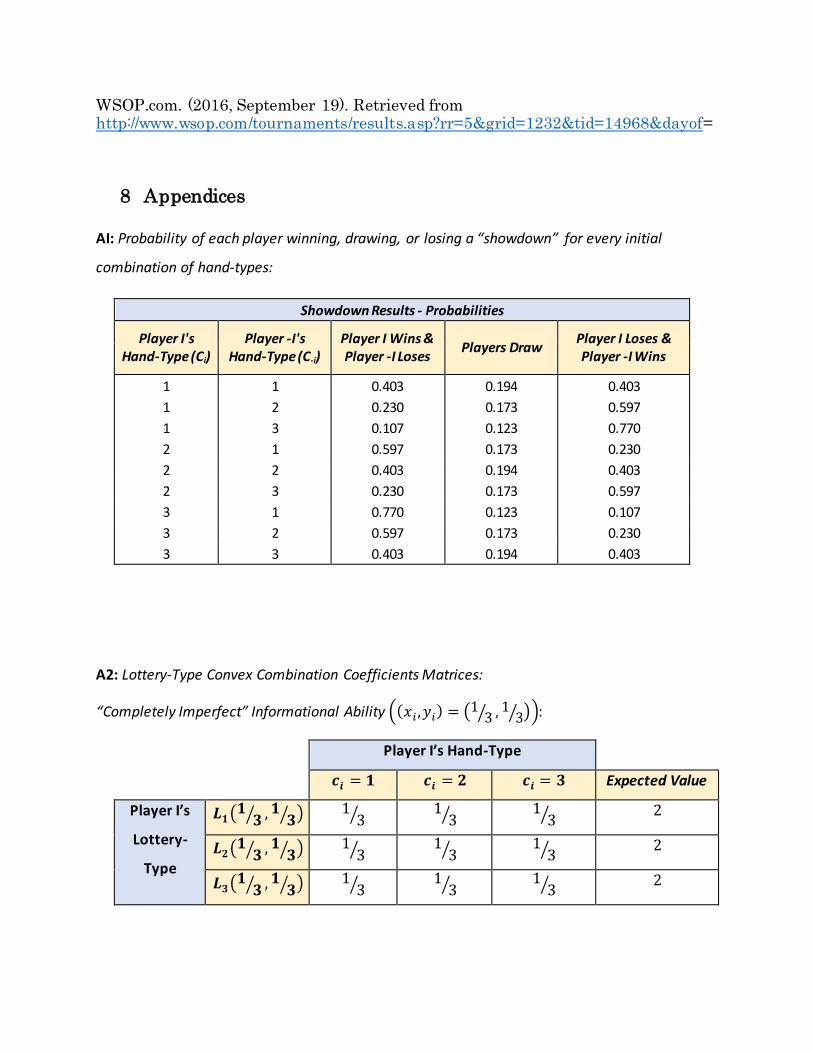
AI: Probability of each player winning, drawing, or losing a “showdown” for every initial

combination of hand-types:

Showdown Results - Probabilities

Player I's Hand-Type (Ci)

Player -I's Hand-Type (C-i)

Player I Wins & Player -I Loses

Players Draw Player I Loses & Player -I Wins

1 1 0.403 0.194 0.403

1 2 0.230 0.173 0.597

1 3 0.107 0.123 0.770

2 1 0.597 0.173 0.230

2 2 0.403 0.194 0.403

2 3 0.230 0.173 0.597

3 1 0.770 0.123 0.107

3 2 0.597 0.173 0.230

3 3 0.403 0.194 0.403

A2: Lottery-Type Convex Combination Coefficients Matrices:

“Completely Imperfect” Informational Ability ((𝑥𝑖 ,𝑦𝑖) = (13⁄ , 1

3⁄ )):


𝒄𝒊 = 𝟏 𝒄𝒊 = 𝟐 𝒄𝒊 = 𝟑 Expected Value

Player I’s

Lottery-

Type

𝑳𝟏(𝟏𝟑⁄ , 𝟏

𝟑⁄ ) 13⁄ 1

3⁄ 13⁄ 2

𝑳𝟐(𝟏𝟑⁄ , 𝟏

𝟑⁄ ) 13⁄ 1

3⁄ 13⁄ 2

𝑳𝟑(𝟏𝟑⁄ , 𝟏

𝟑⁄ ) 13⁄ 1

3⁄ 13⁄ 2

http://www.wsop.com/tournaments/results.asp?rr=5&grid=1232&tid=14968&dayof

“Vague” Informational Ability ((𝑥𝑖 ,𝑦𝑖) = (59⁄ , 5

9⁄ )):



Player I’s

Lottery-

Type

𝑳𝟏(𝟓𝟗⁄ , 𝟓

𝟗⁄ ) 59⁄ 2

9⁄ 29⁄ 5

3⁄

𝑳𝟐(𝟓𝟗⁄ , 𝟓

𝟗⁄ ) 29⁄ 5

9⁄ 29⁄ 2

𝑳𝟑(𝟓𝟗⁄ , 𝟓

𝟗⁄ ) 29⁄ 2

9⁄ 59⁄ 7

3⁄

“Strong” Informational Ability ((𝑥𝑖 ,𝑦𝑖) = (79⁄ , 7

9⁄ )):



Player I’s

Lottery-

Type

𝑳𝟏(𝟕𝟗⁄ , 𝟕

𝟗⁄ ) 79⁄ 1

9⁄ 19⁄ 4

3⁄

𝑳𝟐(𝟕𝟗⁄ , 𝟕

𝟗⁄ ) 19⁄ 7

9⁄ 19⁄ 2

𝑳𝟑(𝟕𝟗⁄ , 𝟕

𝟗⁄ ) 19⁄ 1

9⁄ 79⁄ 8

3⁄

“Perfect” Informational Ability ((𝑥𝑖 ,𝑦𝑖) = (1, 1)):



Player I’s

Lottery-

Type

𝑳𝟏(𝟏,𝟏) 1 0 0 1

𝑳𝟐(𝟏,𝟏) 0 1 0 2

𝑳𝟑(𝟏,𝟏) 0 0 1 3

A3: Informational Ability Coordinates & Constraints – Calibration Plot:

A4: Summary of the cases presented in the Analysis section:

Section Case Number of Subcases

5.2.1 Benchmark 1

5.2.2 Altering the Blind Cost 11

5.2.3 Altering the Players' Initial Capital

Ratio 11

5.2.4 Altering the Players' Skill Level 36

(Xi , Yi ) = (1/3, 1/3)

(Xi , Yi ) = (5/9, 5/9)

(Xi , Yi ) = (7/9, 7/9)

(Xi , Yi ) = (1, 1)

0

0.1

0.2

0.3

0.4

0.5

0.6

0.7

0.8

0.9

1

0 0.1 0.2 0.3 0.4 0.5 0.6 0.7 0.8 0.9 1

Y -

([1

] &

[3

] Lo

tter

y V

alu

es)

X - ([2] Lottery Value)

Informational Ability Coordinates & Constraints

Calibration Parameters Expected Value Constraint Negativity Constraint Xi = Yi

Summer Paper - Terrence Adam Rooney

Documents

Transcript of Summer Paper - Terrence Adam Rooney