Summary Report for Eastern Interior Alaska

Projected Vegetation and Fire Regime Response to Future Climate Change in Alaska

T. Scott Rupp and Anna Springsteen

University of Alaska Fairbanks

Prepared

September 18, 2009

Project Overview This project is part of a statewide model analysis of future vegetation and fire regime response to projected future climate. This work is supported by grants from the National Science Foundation and the Joint Fire Science Program. Additional support has been provided by the UA Scenarios Network for Alaska Planning (SNAP) initiative and from the University of Alaska Fairbanks, US Fish and Wildlife Service, Bureau of Land Management, and the National Park Service. This document provides a summary of preliminary simulation results and a discussion of ongoing modeling activities aimed at providing definitive statewide simulation results. In addition, simulation model details and references are included. Model Simulation Design The design of the model simulations (Fig. 1) provides for the analysis of historical fire activity by two methods: (1) simulating historic fires (1860-2007) based on an empirically derived relationship between climate and fire (Duffy et al. 2005), and (2) linking simulated historic fires (1860-1949), based on the empirical climate-fire relationship, with known fire perimeters (1950-2007; http://agdc.usgs.gov/data/blm/fire/index.html). The historical simulation results for both methods will then be applied to a suite of 6 future climate scenarios (2008-2099) and three emission scenarios (A1B, A1, and B2; see IPCC 2007). This report presents preliminary results for only the A1B emission scenario.

Spinup Historical Future

(1000 yr) 1860 2007 2099

Historical Fire Perimeters 1950-2007

Simulated Fire

(CRU Climate Data 1901-2002)

(PICIR Climate Data 1860-2002)

Simulated Fire

(CRU & PICIR Climate Data 1860-1949)

30 Different Veg/Age Inputs ---Generated by 30 Different Random Climate Permutations (CRU & PICIR Climate Data 1860 – 2002)

CGCM3.1 (Canada

Composite

HADCM3 (UK)

MIROC3.5 (Japan)

GFDL2.1 (US)

ECHAM5 (Germany)

A1 B2 A1B

1950

Spinup Historical Future

(1000 yr) 1860 2007 2099

Historical Fire Perimeters 1950-2007

Simulated Fire

(CRU Climate Data 1901-2002)

(PICIR Climate Data 1860-2002)

Simulated Fire

(CRU & PICIR Climate Data 1860-1949)

30 Different Veg/Age Inputs ---Generated by 30 Different Random Climate Permutations (CRU & PICIR Climate Data 1860 – 2002)

CGCM3.1 (Canada

Composite

HADCM3 (UK)

MIROC3.5 (Japan)

GFDL2.1 (US)

ECHAM5 (Germany)

CGCM3.1 (Canada

Composite

HADCM3 (UK)

MIROC3.5 (Japan)

GFDL2.1 (US)

ECHAM5 (Germany)

A1 B2 A1BA1 B2 A1B

1950 Figure 1 – Schematic showing the model simulation design.

2

The simulation design ultimately allows for statewide simulations (Fig. 2) of both historical simulation methods (2x) to be driven by 6 future climate scenarios (6x) for each of 3 emissions scenarios (3x) for a total of 36 (2x6x3) ensemble runs. Each preliminary ensemble member contains 8 replicated simulations (30 replications to be completed in the final analysis). In all simulations historic climate (1860-2002) was generated using spatially explicit input data from the Climate Research Unit (CRU; http://www.cru.uea.ac.uk/) and the Potsdam Institute for Climate Impact Research (PICIR). The PICAR dataset is a modified version of that presented in Leemans and Cramer (1991). The modification is presented in McGuire et al. (2001). The ‘spin-up’ phase of the modeling generated 30 different initial landscape conditions (vegetation distribution and age structure) at 1860 by using 30 random permutations of historic climate observations from the CRU and PICIR datasets. These landscapes provide the initial (1860) conditions that ALFRESCO uses as input for the simulations. The purpose of the ‘spin-up’ phase is to produce a simulation landscape with realistic patch size and age-class distributions that are generated over multiple fire cycles. Figure 2 – Statewide simulation domain with Eastern Interior boundary identified in red.

3

4

ALFRESCO Model Overview ALFRESCO was originally developed to simulate the response of subarctic vegetation to a changing climate and disturbance regime (Rupp et al. 2000a, 2000b). Previous research has highlighted both direct and indirect (through changes in fire regime) effects of climate on the expansion rate, species composition, and extent of treeline in Alaska (Rupp et al. 2000b, 2001, Lloyd et al. 2003). Additional research, focused on boreal forest vegetation dynamics, has emphasized that fire frequency changes – both direct (climate-driven or anthropogenic) and indirect (as a result of vegetation succession and species composition) – strongly influence landscape-level vegetation patterns and associated feedbacks to future fire regime (Rupp et al. 2002, Chapin et al. 2003, Turner et al. 2003). A detailed description of ALFRESCO can be obtained from the literature (Rupp et al. 2000a, 200b, 2001, 2002). The boreal forest version of ALFRESCO was developed to explore the interactions and feedbacks between fire, climate, and vegetation in interior Alaska (Rupp et al. 2002, 2007, Duffy et al. 2005, 2007) and associated impacts to natural resources (Rupp et al. 2006, Butler et al. 2007). ALFRESCO is a state-and-transition model of successional dynamics that explicitly represents the spatial processes of fire and vegetation recruitment across the landscape (Fig. 3; Rupp et al. 2000a). ALFRESCO does not model fire behavior, but rather models the empirical relationship between growing-season climate (e.g., average temperature and total precipitation) and total annual area burned (i.e., the footprint of fire on the landscape). ALFRESCO also models the changes in vegetation flammability that occur during succession through a flammability coefficient that changes with vegetation type and stand age (Chapin et al. 2003). The fire regime is simulated stochastically and is driven by climate, vegetation type, and time since last fire (Rupp et al. 2000a, 2007). ALFRESCO employs a cellular automaton approach, where an ignited pixel may spread to any of the eight adjacent pixels. ‘Ignition’ of a pixel is determined using a random number generator and as a function of the flammability value of that pixel. Fire ‘spread’ depends on the flammability of the adjacent pixel and any effects of natural firebreaks including non-vegetated mountain slopes and large water bodies, which do not burn. The ecosystem types modeled were chosen as a simple representation of the complex vegetation mosaic occupying the circumpolar arctic and boreal zones. Consequently, ALFRESCO vegetation classes ignore the substantial variation in species composition within these and other intermediate vegetation types. Detailed descriptions of the vegetation states and classification methodology can be found in Rupp et al. (2000a, 2000b, 2001, 2002). The vegetation data used in the model spinup process was derived by reclassifying the 1990 AVHRR vegetation classification (http://agdcftp1.wr.usgs.gov/pub/projects/fhm/vegcls.tar.gz) and the 2001 National Land Cover Database vegetation classification (http://www.mrlc.gov) into the five vegetation classes represented in ALFRESCO (tundra, black spruce, white spruce, deciduous, and dry grassland). Currently, the dry grassland ecosystem type represented in ALFRESCO occurs only locally and at a scale masked by the model’s 1 x 1 km pixel resolution. Differences among tundra vegetation types recognized in the vegetation classifications were ignored, and all tundra types were lumped together as a single tundra class. The actual spruce-canopy level was determined using growing-season climate thresholds.

Remotely sensed satellite data are currently unable to distinguish species-level differences between black and white spruce. We therefore stratified spruce forest using deterministic rules related to topography (i.e., aspect, slope position, and elevation) and growing-season climate. Aspect and slope were used to identify ‘typical’ black spruce forest sites (i.e., poorly drained and northerly aspects) throughout the study region. Growing-season climate and elevation were used primarily to distinguish treeline white spruce forest. In addition, we used growing-season climate thresholds to distinguish young deciduous forest stands from tall shrub tundra. These deterministic rules were also used to denote the climax vegetation state (i.e., black or white spruce forest) for each deciduous pixel. In other words, the rules were used to predetermine the successional trajectory of each deciduous pixel. In this manner, we were able to develop an input vegetation data set that best related the original remotely sensed data into the five vegetation types represented by ALFRESCO, based on a sensible ecological foundation.

Climate• GS Temp.• GS Precip.• Drought

Disturbance• Fire• Insects• Browsing

Deciduous Forest

Black Spruce Forest

Upland Tundra

Dry Grassland

White Spruce Forest

Col

oniz

atio

n

Fire

+ E

xtre

me

Col

d

Extreme ColdFi

re +

Dro

ught

Succession

Fire

Fire + D

rough

t

Fire + Drought

Fire

+ S

eed

Sour

ce

Fire

Succession

Fire + E

xtreme C

old

Fire Fire Fire

Fire Fire

Climate• GS Temp.• GS Precip.• Drought

Disturbance• Fire• Insects• Browsing

Deciduous Forest

Black Spruce Forest

Upland Tundra

Dry Grassland

White Spruce Forest

Col

oniz

atio

n

Fire

+ E

xtre

me

Col

d

Extreme ColdFi

re +

Dro

ught

Succession

Fire

Fire + D

rough

t

Fire + Drought

Fire

+ S

eed

Sour

ce

Fire

Succession

Fire + E

xtreme C

old

FireFire FireFire FireFire

FireFire FireFire

Figure 3 – Conceptual model of vegetation states (colored boxes), possible transitions (arrows), and driving processes/factors responsible for the rate and direction of transitions (arrow labels). Dynamic treeline transitions and the dry grassland state were not activated for the preliminary simulations. Version 1.0.5 can operate at several time steps and pixel resolutions, however the current model calibration and parameterization was conducted at an annual time step and 1 km2 pixel resolution. A 30 m2 calibration and parameterization is currently underway. Other model developments include refined tundra transition stages, fire suppression effects on fire size, simulated fire severity patterns and fire severity effects on successional rates and trajectories. A new version of the boreal ALFRESCO simulation model with these developments will be available beginning in 2010.

5

6

Driving Climate Products The simulation design for this project utilizes climate projections that have been assessed and downscaled by the UA Scenarios Network for Alaska Planning (SNAP). Use of GCMs to model future climate General Circulation Models (GCMs) are the most widely used tools for projections of global climate change over the timescale of a century. Periodic assessments by the Intergovernmental Panel on Climate Change (IPCC) have relied heavily on GCM simulations of future climate driven by various emission scenarios. The IPCC uses complex coupled atmospheric and oceanic GCMs. These models integrate multiple equations, typically including surface pressure; horizontal layered components of fluid velocity and temperature; solar short wave radiation and terrestrial infra-red and long wave radiation; convection; land surface processes; albedo; hydrology; cloud cover; and sea ice dynamics. GCMs include equations that are iterated over a series of discrete time steps as well as equations that are evaluated simultaneously. Anthropogenic inputs such as changes in atmospheric greenhouse gases can be incorporated into stepped equations. Thus, GCMs can be used to simulate the changes that may occur over long time frames due to the release of greenhouse gases into the atmosphere. Greenhouse gas-driven climate change represents a response to the radiative forcing associated with increases of carbon dioxide, methane, water vapor and other gases, as well as associated changes in cloudiness. The climate response can vary widely among models because it is strongly modified by feedbacks involving clouds, the cryosphere, water vapor and other processes whose effects are not well understood. Changes in the radiative forcing associated with increasing greenhouse gases have thus far been small relative to existing seasonal cycles. Thus, the ability of a model to accurately replicate seasonal radiative forcing is a good test of its ability to predict anthropogenic radiative forcing. Model Selection Different coupled GCMs have different strengths and weaknesses, and some can be expected to perform better than others for northern regions of the globe. SNAP principle investigator Dr. John Walsh and colleagues evaluated the performance of a set of fifteen global climate models used in the Coupled Model Intercomparison Project. Using the outputs for the A1B (intermediate) climate change scenario, they calculated the degree to which each model’s output concurred with actual climate data for the years 1958-2000 for each of three climatic variables (surface air temperature, air pressure at sea level, and precipitation) for three overlapping regions (Alaska only, 60-90 degrees north latitude, and 20-90 degrees north latitude). The core statistic of the validation was a root-mean-square error (RMSE) evaluation of the differences between mean model output for each grid point and calendar month, and data from the European Centre for Medium-Range Weather Forecasts (ECMWF) Re-Analysis, ERA-40. The ERA-40 directly assimilates observed air temperature and sea level pressure observations into a product spanning 1958-2000. Precipitation is

computed by the model used in the data assimilation. The ERA-40 is one of the most consistent and accurate gridded representations of these variables available. To facilitate GCM intercomparison and validation against the ERA-40 data, all monthly fields of GCM temperature, precipitation and sea level pressure were interpolated to the common 2.5° × 2.5° latitude–longitude ERA-40 grid. For each model, Walsh and colleagues calculated RMSEs for each month, each climatic feature, and each region, then added the 108 resulting values (12 months x 3 features x 3 regions) to create a composite score for each model (Table 1). A lower score indicated better model performance.

Table 1 – Component and overall ranking of the 15 GCMs evaluated from the IPCC 4th assessment. The top five models were chosen as performing best over Alaska. GCMs that performed best over the larger domains tended to be the ones that performed best over Alaska. Although biases in the annual mean of each model typically accounted for about half of the models’ RMSEs, the systematic errors differed considerably among the models. There was a tendency for the models with the smaller errors to simulate a larger greenhouse warming over the Arctic, as well as larger increases of Arctic precipitation and decreases of Arctic sea level pressure when greenhouse gas concentrations are increased. Since several models had substantially smaller systematic errors than the other models, the differences in greenhouse projections implied that the choice of a subset of models might offer a viable approach to narrowing the uncertainty and obtaining more robust estimates of future climate change in regions such as Alaska. Thus, SNAP selected the five best-performing models out of the fifteen: MPI_ECHAM5, GFDL_CM2_1, MIROC3_2_MEDRES, UKMO_HADCM3, and CCCMA_CGCM3_1. These five models are used to generate climate projections independently, as well as in combination (i.e., composite), in order to further reduce the error associated with dependence on a single model.

7

8

Downscaling model outputs Because of the mathematical complexity of GCMs, they generally provide output at coarse spatial resolutions, with grid cells typically 1°-5° latitude and longitude. For example, the standard resolution of HadCM3 is 1.25 degrees in latitude and longitude, with 20 vertical levels, leading to approximately 1,500,000 variables. Finer scale projections of future conditions are not directly available. However, local topography can have profound effects on climate at much finer scales, and almost all land management decisions are made at much finer scales. Thus, some form of downscaling is necessary in order to make GCMs useful tools for regional climate change planning. Historical climate data estimates at 2 km resolution are available from PRISM (Parameter-elevation Regressions on Independent Slopes Model), which was originally developed to address the lack of climate observations in mountainous regions or rural areas. PRISM uses point measurements of climate data and a digital elevation model to generate estimates of annual, monthly and event-based climatic elements. Climatic elements for each grid cell are estimated via multiple regression using data from many nearby climate stations. Stations are weighted based on distance, elevation, vertical layer, topographic facet, and coastal proximity. PRISM offers data at a fine scale that is useful to land managers and communities, but it does not offer climate projections. Thus, SNAP needed to link PRISM to the GCM outputs. This work was also performed by PI Walsh and colleagues. They first calculated mean monthly precipitation and mean monthly surface air temperature for PRISM grid cells for 1961-1990, creating PRISM baseline values. Next, they calculated GCM baseline values for each of the five selected models using mean monthly outputs for 1961-1990. They then calculated differences between projected GCM values and baseline GCM values for each year out to 2099 and created “anomaly grids” representing these differences. Finally, they added these anomaly grids to PRISM baseline values, thus creating fine-scale (2 km) grids for monthly mean temperature and precipitation for every year out to 2099. This method effectively removed model biases while scaling down the GCM projections.

Driving Climate Summary

Statewide-specific climate data can now be accessed through SNAP (www.snap.uaf.edu) in tabular form, as graphs, or as maps (GIS layers and KML files) depicting the whole state of Alaska or part of the state. Currently, tables or graphs of mean monthly temperature and precipitation projections by decade are available for 353 communities in Alaska. Statewide GIS layers of mean monthly temperature and total precipitation for each year out to 2099 are also available and were used to develop the input data sets used in this project. The following time series graphs and maps provide examples of the types of summary information that can be generated for any defined region within the state. The remainder of this report will focus on the Eastern Interior simulation domain (see red area in Fig. 3). The majority of the figures presented will be for the ECHAM5 and CGCM3.1 models, which represent the most severe and least severe scenarios of future warming, respectively, and the GCM Composite model, which represents the least biased and most mid-range projection.

1900 1950 2000 2050 2100

-50

51

0

Year

Ma

rch

thru

Ju

ne

Me

an

Te

mp

era

ture

(ºC

)

CRU + GCM CompositeECHAM5HADCM3MIROC3.2GFDL2.1CGCM3.1

Figure 4 – Time series of average March thru June temperature (ºC) integrated across the Eastern Interior domain for the historical climate (CRU), the five downscaled GCMs, and the GCM Composite model.

9

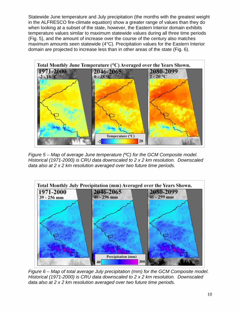
Statewide June temperature and July precipitation (the months with the greatest weight in the ALFRESCO fire-climate equation) show a greater range of values than they do when looking at a subset of the state, however, the Eastern Interior domain exhibits temperature values similar to maximum statewide values during all three time periods (Fig. 5), and the amount of increase over the course of the century also matches maximum amounts seen statewide (4°C). Precipitation values for the Eastern Interior domain are projected to increase less than in other areas of the state (Fig. 6).

Figure 5 – Map of average June temperature (ºC) for the GCM Composite model. Historical (1971-2000) is CRU data downscaled to 2 x 2 km resolution. Downscaled data also at 2 x 2 km resolution averaged over two future time periods.

Figure 6 – Map of total average July precipitation (mm) for the GCM Composite model. Historical (1971-2000) is CRU data downscaled to 2 x 2 km resolution. Downscaled data also at 2 x 2 km resolution averaged over two future time periods.

10

Model Simulation Results Model Simulation Results We currently hold the most confidence in the simulation results for the interior region of Alaska, which includes the Eastern Interior domain. We are in the process of further development and refinement of the tundra vegetation state (JFSP funded project with NPS), and further development and implementation of a grassland frame (USFWS funded), which will also improve our confidence in the simulation results for this region and in other areas of the state. Interpretation of the simulation results should consider two major sources of uncertainty: (1) both the climate projections and the validity of ALFRESCO model assumptions regarding successional trajectories become less certain the farther into the future we consider, and (2) due to the stochastic nature of both ignitions and firespread within ALFRESCO it is not possible to simulate the exact geographic location of future fire occurrence or vegetation type.

We currently hold the most confidence in the simulation results for the interior region of Alaska, which includes the Eastern Interior domain. We are in the process of further development and refinement of the tundra vegetation state (JFSP funded project with NPS), and further development and implementation of a grassland frame (USFWS funded), which will also improve our confidence in the simulation results for this region and in other areas of the state. Interpretation of the simulation results should consider two major sources of uncertainty: (1) both the climate projections and the validity of ALFRESCO model assumptions regarding successional trajectories become less certain the farther into the future we consider, and (2) due to the stochastic nature of both ignitions and firespread within ALFRESCO it is not possible to simulate the exact geographic location of future fire occurrence or vegetation type. Empirical Climate-Fire RelationshipEmpirical Climate-Fire Relationship

1900 1950 2000 2050 2100

46

81

01

2

Year

Bo

rea

l AL

FR

ES

CO

Fir

e C

lima

te E

qn

Boreal ALFRESCO FireClimate Relationship

CRUCompositeECHAM5CGCM3.1

The ALFRESCO model was driven by spatially explicit datasets of observed and projected monthly temperature and precipitation (see Model Simulation Design section) – March through June monthly average temperature and June and July total precipitation. Based on future projections we expect climatic effects alone to result in substantial increases (as much as 50%) in landscape flammability across all 5 climate scenarios at the statewide scale (Fig. 7). For this study area, we expect a similar increase; the Eastern Interior domain is located in a region that matches the maximum statewide temperature increase of 4°C by the end of the century. Precipitation is also expected to increase, however in Interior Alaska, this increase is likely not sufficient to counte ct increased evapotranspiration and general drying caused by higher temper tures, and this holds true in the Eastern Interior domain, as well.

raa

Land

scap

e F

lam

mab

ility

sc

ape

Fla

mm

abili

ty

Figure 7 – Time series showing climatic influence on statewide landscape flammability across all vegetation types. CRU observational data (black circles) and the GCM Composite future climate (yellow circles); ECHAM5 (red dashed line) represents the greatest warming scenario; CGCM3.1 (purple dashed line) represents the least warming scenario. Black dashed line is 10-yr running average.

11

One factor that may potentially confound the interpretation of these future results is the potential for the boreal forest ecosystem to dramatically change. For example, one of the likely consequences of future climate change appears to be a significant increase in the amount of burning. This elevated burning results in a shift from conifer dominance to deciduous dominance across interior Alaska. Since the regression linking climate to fire was developed based on a forest structure that was dominated by coniferous vegetation, it is likely that the form of this relationship will change following a shift in the dominant forest vegetation type. Historical Simulations The preliminary results presented in this section of the report cover only simulated historic fires (1860-2007) based on an empirically derived relationship between climate and fire (Duffy et al. 2005; see Empirical Climate-Fire Relationship section). The ALFRESCO model performed well simulating historical landscape dynamics that closely followed observed fire regime and vegetation cover characteristics. This assessment is made based on a number of different calibration metrics that compare simulated data to various aspects of the fire regime (e.g. fire size distribution, frequency-area distribution, cumulative area burned). Cumulative area burned is consistent with observed area burned from 1950-2007 (Fig. 8). In general, ALFRESCO estimates cumulative area burned well in the Eastern Interior domain. Differences in simulated and observed cumulative area burned occur primarily because we are unable to accurately simulate the 1950, 2004, and 2005 fire seasons.

1950 1960 1970 1980 1990 2000

020000

40000

600

00

80000

Year

Cum

alit

ive A

rea B

urn (k

m^2

)

HistoricalSingle Rep

CAB vs Time (1950:2007)

Figure 8 – Comparison of historical (black line) and simulated (grey lines) cumulative area burned (km2) from 1950-2007. The solid line represents the historical burns and the dashed lines represent individual replicate results (n=100).

12

1900 1950 2000

05

00

01

000

01

500

02

000

0

Year

cells

bu

rn

AreaBurn/Year: Replicate 3

Simulated AB/YearHistorical AB/Year

In the Eastern Interior region, ALFRESCO performed well simulating both the total annual area burned and the overall magnitude of high and low fire season variability (Fig. 9), as well as simulating the spatial distribution of fires across the landscape (Fig. 10). Correlations between simulated and historical (1950-2007) fire activity ranged from 0.35-0.60, with a mean of 0.47. Figure 9 – Historical observed (orange boxes) versus simulated (red circles) total annual area burned. Simulation results from the best single replicate out of 100 (replicate 3).

Figure 10 – Map showing observed fire perimeters (left panel) and simulated fire perimeters (right panel). Color scale indicates time since last fire (darker red equals more recent fires). Simulated results from the best single replicate (replicate 3). The region identified by the black outline identifies the Eastern Interior boundary.

13

The ALFRESCO model also performed well simulating general vegetation composition across the landscape. Model simulations suggest a long-term co-dominance of conifer and deciduous forests in the region (Fig. 11). Remotely sensed data provides two snapshots in time, 1990 and 2001, from which we can directly compare proportion of conifer to deciduous (Fig. 12). The ALFRESCO ratio at the1990 time slice was slightly off when compared to the observed remote sensing data, but the simulated conifer-to-deciduous ratio was a closer in 2001 (1990 observed ratio = 3.4 versus 1990 simulated ratio = 2.3; 2001 observed ratio = 1.3 versus 2001 simulated ratio = 1.5).

1900 1950 2000

60000

80000

100000

120000

Year

Vegeta

tion(1

km^2

)

ConiferDecid

14

Figure 11 – Time series showing the total simulated amount of conifer (green line) versus deciduous (brown line) vegetation 1860-2007 across interior Alaska. AVHRR classification (http://agdcftp1.wr.usgs.gov/pub/projects/fhm/vegcls.tar.gz) at 1990 and the National Land Cover Database (http://www.mrlc.gov) at 2001.

2001

1990

Figure 12 – Observed versus simulated vegetation maps from the single best replicate at two years: 1990 and 2001.

The 2001 observed ratio is based on the NCLD vegetation image, which is more recent with a finer resolution, hence greater weight is put on ALFRESCO simulations matching the 2001 observed ratio, which it does fairly well for Eastern Interior area. For example, in Figure 11, you can see deciduous inclusions within the black spruce patch that were not able to be included in the larger resolution 1990 observed ratio image. Future Projections The success of ALFRESCO in simulating historical observations when driven with historical climate provides a degree of confidence that allows us to simulate into the future, driving the simulations with projected climate scenarios, and to use that information to make inferences about future landscape structure and function. ALFRESCO simulations suggest in general an increase in cumulative area burned through 2099 (Fig. 13). However, individual climate scenarios produced slightly different simulated fire activity. ECHAM5 and MIROC3.5 GCM scenarios produced the largest simulated changes in fire activity, whereas GFDL2.1 and HADCM3 produced more moderate changes in simulated fire activity. CGCM3.1 produced the least simulated future fire activity. Individual replicate simulations also show a pattern of less frequent interannual periods of low fire activity (Figs. 14-16). These simulations are generally consistent with the statewide simulations.

1950 2000 2050 2100

05

00

00

10

00

00

15

00

00

Year

Cu

ma

litiv

e A

rea

Bu

rn (

km^2

)

Historical FireCRU + GCM CompositeECHAM5HADCM3MIROC3.5GFDL2.1CGCM3.1

Figure 13 – Time series graph showing simulated cumulative area burned (km2) through 2099 for historical observations (black line), simulated historical (dark green line), and the five GCM scenarios plus the GCM Composite scenario (also dark green line).

15

1950 2000 2050 2100

05

000

100

00

15

00

020

00

0

Year

Are

a B

urn

(km

^2)

AreaBurn/Year: Replicate 12

Simulated AB/YearHistorical AB/Year

Figure 14– Time series graph showing simulated fire activity for a single replicate simulation of the CGCM3.1 climate scenario.

1950 2000 2050 2100

05

000

100

00

15

00

020

00

0

Year

Are

a B

urn

(km

^2)

AreaBurn/Year: Replicate 2

Simulated AB/YearHistorical AB/Year

Figure 15 – Time series graph showing simulated fire activity for a single replicate simulation of the GCM Composite climate scenario.

16

1950 2000 2050 2100

05000

10000

15000

20000

Year

Are

a B

urn

(km

^2)

AreaBurn/Year: Replicate 76

Simulated AB/YearHistorical AB/Year

Figure 16– Time series graph showing simulated fire activity for a single replicate simulation of the ECHAM5 climate scenario.

Figure 17 – Map showing time since last fire (TSLF) for the period 2008-2099 for the CGCM3.1, GCM Composite, and ECHAM5 climate scenarios.

17

The simulated response of vegetation to increased burning, especially in the earlier half of the 21st century (Fig. 17), suggests the potential for a substantial shift in the future proportion of conifer and deciduous forest on the landscape (Fig. 18 and 19), with some scenarios showing a greater shift towards deciduous dominance than others. The magnitude of the shift differs from the most warming scenario (ECHAM5; Fig. 20 and 21) to the mid-range warming scenario to, finally, the least warming scenario, where it eventually reverses at the end of the century (CGCM3.1; Fig. 22 and Fig. 23).

1900 1950 2000 2050 2100

60

000

80

000

10

000

012

00

00

Ve

geta

tion(

1km

^2)

ConiferDecid

Figure 18– Time series for the GCM Composite climate scenario showing the total simulated amount of conifer (green line) versus deciduous (brown line) vegetation 1860-2099 based on the mean of replicates (n=100).

Figure 19– Vegetation map from a single replicate of the GCM Composite climate scenario showing the simulated distribution of vegetation types across the landscape. Full page maps of years 2000 and 2025 are provided in Appendix A.

18

1900 1950 2000 2050 2100

60

00

08

00

00

10

00

00

12

00

00

Year2

Ve

ge

tatio

n(1

km^2

)

ConiferDecid

Figure 20– Time series for the ECHAM5 climate scenario showing the total simulated amount of conifer (green line) versus deciduous (brown line) vegetation 1860-2099 based on the mean of replicates (n=100).

Figure 21 – Vegetation map from a single replicate of the ECHAM5 climate scenario showing the simulated distribution of vegetation types across the landscape. Full page maps of years 2000 and 2025 are provided in Appendix A.

19

1900 1950 2000 2050 2100

60

00

08

00

00

10

00

00

12

00

00

Year2

Ve

ge

tatio

n(1

km^2

)

ConiferDecid

Figure 22 – Time series for the CGCM3.1 climate scenario showing the total simulated amount of conifer (green line) versus deciduous (brown line) vegetation 1860-2099 based on the mean of replicates (n=100).

Figure 23– Vegetation map from a single replicate of the CGCM3.1 climate scenario showing the simulated distribution of vegetation types across the landscape. Full page maps of years 2000 and 2025 are provided in Appendix A. 20

An alternate method to analyze the simulated potential shift in vegetation composition towards deciduous vegetation dominance is to identify places across the simulation domain that are most frequently simulated as deciduous vegetation through time. Based on this methodology we identified shifts toward more frequently simulated deciduous vegetation as early as 2025 and 2050 in all three models (Figs. 24 – 26).

Figure 24– The GCM Composite climate scenario showing the simulated distribution of deciduous vegetation across the landscape.

21

Figure 25– The ECHAM5 climate scenario showing the simulated distribution of deciduous vegetation across the landscape.

Figure 26– The CGCM3.1 climate scenario showing the simulated distribution of deciduous vegetation across the landscape.

22

Along with this potential vegetation shift, we can utilize simulation output of vegetation type and time since last fire (i.e., stand age) to develop potential habitat metrics. For example, Rupp et al. (2006) analyzed the potential change in total amount of winter habitat for the Nelchina caribou herd using an algorithm to track preferred vegetation type (spruce forest and woodland spruce stands) and age class (> 80 yr). Other metrics could be developed and implemented as part of the post-processing of the simulation output. Below are examples for caribou winter habitat (following Rupp et al. 2006) as well as moose habitat. Moose habitat in this example is defined as deciduous vegetation between 10 and 30 yr (based on Maier et al. 2005).

1900 1950 2000 2050 2100

05

00

00

15

00

00

Caribou Winter Habitat

Year

Sp

ruce

> 8

0 (

km^2

)

1900 1950 2000 2050 2100

05

00

00

15

00

00

Moose Habitat

Year

10

<D

eci

d<

31

(km

^2)

Figure 27 – Habitat graphs showing how habitat for caribou (spruce > 80 yr) and moose (deciduous between 10 and 30 yr) are projected to change with the simulated fire activity in the GCM Composite climate scenario.

23

1900 1950 2000 2050 2100

05

00

00

15

00

00

Caribou Winter Habitat

Year

Sp

ruce

> 8

0 (

km^2

)

1900 1950 2000 2050 2100

05

00

00

15

00

00

Moose Habitat

Year

10

<D

eci

d<

31

(km

^2)

Figure 28– Habitat graphs showing how habitat for caribou (spruce > 80 yr) and moose (deciduous between 10 and 30 yr) are projected to change with the simulated fire activity in the ECHAM5 climate scenario.

1900 1950 2000 2050 2100

05

00

00

15

00

00

Caribou Winter Habitat

Year

Sp

ruce

> 8

0 (

km^2

)

1900 1950 2000 2050 2100

05

00

00

15

00

00

Moose Habitat

Year

10

<D

eci

d<

31

(km

^2)

24

Figure 29 – Habitat graphs showing how habitat for caribou (spruce > 80 yr) and moose (deciduous between 10 and 30 yr) are projected to change with the simulated fire activity in the CGCM3.1 climate scenario.

Due to the stochastic nature of the ALFRESCO model (see ALFRESCO Model Overview) the simulated vegetation characteristics (e.g., type and age) do not provide a direct predication of where a fire or specific vegetation type will occur. However, by looking at many replicates together, maps can be made of where fire activity or a specific vegetation type is most likely to occur. An example provides an analysis of how many times each 1 km grid cell burns through time and across replicates. This value can then be divided by the number of replicates and the number of years to create a fire risk map for that time frame – i.e., the probability of any given cell burning in any one year. The inverse of that probability is the fire return interval. The following three probability maps (Figs. 30 - 32) show the ECHAM5 climate model produces the highest probabilities of fire occurrence across all areas of the Eastern Interior domain (Fig. 30). They correspond well with the frequency maps of simulated areas of deciduous vegetation in 2025 and 2050 (Figs. 24 – 26). They also show the shortest return intervals are likely to happen during the earlier half of this century (Fig. 31).

Figure 30 – Maps showing the probability of a cell burning during any one year 2001-2099. Probabilities derived from 100 replicates.

25

Figure 31 - Maps showing the probability of a cell burning during any one year 2001-2050. Probabilities derived from 100 replicates.

Figure 32 - Maps showing the probability of a cell burning during any one year 2051-2099. Probabilities derived from 100 replicates.

26

27

Summary of Preliminary Simulation Results and Management Implications Preliminary results from the statewide simulations identify consistent trends in projected future fire activity and vegetation response. The simulation results strongly suggest that boreal forest vegetation will change dramatically from the spruce dominated landscapes of the last century. The Eastern Interior simulation results produced these same general trends in projected future fire activity and vegetation. The ALFRESCO model simulations suggest a general increase in fire activity through the end of this century (2099) in response to projected warming temperatures and less available moisture. Changes in the projected cumulative area burned suggest the next 20-30 years will experience the most rapid change in fire activity and the associated changes in vegetation dynamics. Simulations of future fire activity suggest more frequent large to moderate fire seasons and an increase in magnitude and periodicity of small fire seasons; hence there will be a decrease in the interannual variability of annual area burned. Differences do exist among climate scenarios providing multiple possible futures that must be considered within the context of land and natural resource management. For example, the climate model ECHAM5 shows a much more distinct vegetation shift from coniferous to deciduous dominance by 2025 and much higher fire risks than the other models. Increased deciduous dominance on the landscape will contribute to a probable change in the patch dynamics between vegetation types and age. The simulation results suggest that this change may reach an equilibrium stage where the patch dynamics may self-perpetuate for many decades if not centuries in some models, but may switch back in others. In spite of the shift towards less flammable age classes and towards deciduous species, the simulation results indicate that there will be more frequent fires burning; resulting in an overall increase in area burned annually. These two results appear to drive the simulated change in landscape dynamics where increased landscape flammability, driven by climate change, modifies landscape-level vegetation (i.e., fuels) distribution and pattern, which in turn feeds back to future fire activity by reducing flammable vegetation patch size (i.e., fuel continuity). Decisions made by fire and land managers during this current period of rapid change will influence the structure and pattern of vegetation across the boreal forest in Alaska. The Eastern Interior domain lies in an area expected to be one of the greatest areas of change in the state. The central portion of the simulation area showed the highest fire risk in the near future (see Figs 30-32). Fire managers should consider how land management objectives may be affected by the predicted changes to natural fire on the landscape. The Boreal ALFRESCO model can be used to simulate how changes in fire management may change the potential future landscape. It can also be used to assess how particular vegetation age classes (i.e., deciduous forest 10-30 years old) that may represent habitat conditions for important wildlife resources may be affected by the fire, vegetation and climate interactions predicted into the future. Acknowledgements We want to thank Jennifer Schmidt, Mark Olson, Dr. Paul Duffy, and Tim Glaser for their determined work and attention to detail in parameterizing and analyzing both the statewide and refuge specific simulations and assisting in the preparation of this report. Ben Kennedy (BLM) provided critical input throughout this project.

28

ALFRESCO Model References BUTLER, L.G., K. KIELLAND, T.S. RUPP, AND T.A. HANLEY. 2007. Interactive controls by

herbivory and fluvial dynamics over landscape vegetation patterns along the Tanana River, interior Alaska. Journal of Biogeography. 34:1622-1631.

DUFFY, P., J. EPTING, J.M. GRAHAM, T.S. RUPP, AND A.D. McGuire. 2007. Analysis of Alaskan fire severity patterns using remotely sensed data. International Journal of Wildland Fire. 16:277-284.

RUPP, T.S., X. CHEN, M. OLSON, AND A.D. McGUIRE. 2007. Sensitivity of simulated land cover dynamics to uncertainties in climate drivers. Earth Interactions. 11(3):1-21.

HU, F.S., L.B. BRUBAKER, D.G. GAVIN, P.E. HIGUERA, J.A. LYNCH, T.S. RUPP, AND W. TINNER. 2006. How climate and vegetation influence the fire regime of the Alaskan boreal biome: the Holocene perspective. Mitigation and Adaptation Strategies for Global Change (MITI). 11(4):829-846.

RUPP, T.S., OLSON, M., HENKELMAN, J., ADAMS, L., DALE, B., JOLY, K., COLLINS, W., and A.M. STARFIELD. 2006. Simulating the influence of a changing fire regime on caribou winter foraging habitat. Ecological Applications. 16(5):1730-1743.

CHAPIN, F.S., III, M. STURM, M.C. SERREZE, J.P McFADDEN, J.R. KEY, A.H. LLOYD, A.D. McGUIRE, T.S. RUPP, A.H. LYNCH, J.P SCHIMEL, J. BERINGER, W.L. CHAPMAN, H.E. EPSTEIN, E.S. EUSKIRCHEN, L.D. HINZMAN, G. JIA, C.L. PING, K.D. TAPE, C.D.C. THOMPSON, D.A. WALKER, and J.M. WELKER. 2005. Role of Land-Surface Changes in Arctic Summer Warming. Science. Published online September 22 2005; 10.1126/science.1117368 (Science Express Reports).

DUFFY, P.A., J.E. WALSH, J.M. GRAHAM, D.H. MANN, and T.S. RUPP. 2005. Impacts of the east Pacific teleconnection on Alaskan fire climate. Ecological Applications. 15(4):1317-1330.

LLOYD, A., T.S. RUPP, C. FASTIE, and A.M. STARFIELD. 2003. Patterns and dynamics of treeline advance on the Seward Peninsula, Alaska. Journal of Geophysical Research - Atmospheres. 108(D2):8161, DOI: 10.1029/2001JD00852.

CHAPIN, F.S., III, T.S. RUPP, A.M. STARFIELD, L. DeWILDE, E.S. ZAVALETA, N. FRESCO, J. HENKELMAN, and A.D. McGUIRE. 2003. Planning for resilience: modeling change in human-fire interactions in the Alaskan boreal forest. Frontiers in Ecology and the Environment. 1(5):255-261.

TURNER, M.G., S.L. COLLINS, A.L. LUGO, J.J. MAGNUSON, T.S. RUPP, and F.J. SWANSON. 2003. Disturbance Dynamics and Ecological Response: The Contribution of Long-term Ecological Research. BioScience. 53(1)46-56.

RUPP, T.S., A.M. STARFIELD, F.S. CHAPIN III, and P. DUFFY. 2002. Modeling the impact of black spruce on the fire regime of Alaskan boreal forest. Climatic Change 55: 213-233.

RUPP, T.S., R.E. KEANE, S. LAVOREL, M.D. FLANNIGAN, and G.J. CARY. 2001. Towards a classification of landscape-fire-succession models. GCTE News 17: 1-4.

RUPP, T.S., F.S. CHAPIN III, and A.M. STARFIELD. 2001. Modeling the influence of topographic barriers on treeline advance of the forest-tundra ecotone in northwestern Alaska. Climatic Change 48: 399-416.

RUPP, T.S., A.M. STARFIELD, and F.S. CHAPIN III. 2000. A frame-based spatially explicit model of subarctic vegetation response to climatic change: comparison with a point model. Landscape Ecology 15: 383-400.

RUPP, T.S., F.S. CHAPIN III, and A.M. STARFIELD. 2000. Response of subarctic vegetation to transient climatic change on the Seward Peninsula in northwest Alaska. Global Change Biology 6: 451-455.

APPENDIX A – Full-Page Simulated Vegetation Maps 29

30

31

32

33

34