1

Forecasting the response of Klamath Basin Chinook populations to dam removal and restoration of anadromy versus no action Noble Hendrix R2 Resource Consultants, Inc. 15250 NE 95th Street Redmond, WA 98052-2518 E-mail: nhendrix@r2usa.com September 20, 2011

2

Abstract

Two alternative actions are being evaluated in the Klamath Basin: 1) a No Action Alternative (NAA) and 2) removal of four mainstem dams (Iron Gate, Copco I, Copco II, and J.C. Boyle) and initiation of habitat restoration in the Klamath Basin under a Dam Removal Alternative (DRA). The decision process regarding which action to implement requires annual forecasts of abundance with uncertainty under each of the two alternatives from 2012 to 2061. I forecasted escapement for both alternatives by constructing a life-cycle model (Evaluation of Dam Removal and Restoration of Anadromy, EDRRA) composed of: 1) a stock recruitment relationship between spawners and age 3 in the ocean, which is when they are vulnerable to the fishery, and 2) a fishery model that calculates harvest, maturation, and escapement. To develop stage 1 of the model under NAA, I estimated the historical stock recruitment relationship in the Klamath River below Iron Gate Dam in a Bayesian framework. To develop stage 1 of the model under DRA, I used the predictive spawner recruitment relationships in Liermann et al. (2010) to forecast recruitment to age 3 from tributaries to Upper Klamath Lake, which is the site of active reintroduction of anadromy. I also modified the spawner recruit relationship under DRA to include additional spawning capacity between Iron Gate Dam and Keno Dam. In order to facilitate the comparison of the two alternatives, I used paired Monte Carlo simulations to forecast the levels of escapement and harvest under NAA and DRA. Median escapements and harvest were higher in DRA relative to NAA with a high degree of overlap in 95% confidence intervals due to uncertainty in stock-recruitment dynamics. Still, there was a 0.75 probability of higher annual escapement and a 0.7 probability of higher annual harvest by performing DRA relative to NAA, despite uncertainty in the abundance forecasts. The median increase in escapement in the absence of fishing was 81.4% (95% symmetric probability interval [95%CrI]: -59.9%, 881.4%), the median increase in ocean harvest was 46.5% (95%CrI: -68.7, 1495.2%), and the median increase in tribal harvest was 54.8% (95%CrI: -71.0%, 1841.0%) by performing DRA relative to NAA (estimates provided for model runs after 2033 when portion of the population in the tributaries to UKL are assumed to be established and Iron Gate Hatchery production has ceased).

3

1 Introduction

Evaluation of alternative actions in light of imperfect information is a dilemma commonly faced by decision makers (Berger 2006; Raifa and Sclaifer 2000). Often, there is a mismatch between the time needed to amass information through studies to provide a body of evidence for one action versus another (long time frame) and the time over which a decision is needed (short time frame). Modeling is a critical step in the decision making process and is useful for evaluating the outcome of each action, the uncertainty in the outcomes, and how those relate to the decision maker’s objectives (Clemen 1996). Analyses that can improve the predictive ability of such models, such as statistical analysis, are valuable in revealing and quantifying some of the uncertainties in the decision process. Bayesian statistical analyses are particularly well suited to decision analysis given their natural approach to modeling uncertainty (Berger 2006). In the report that follows, I conducted a series of Bayesian statistical analyses and performed model forecasts in support of a decision: whether to operate the series of dams on the Klamath River consistent with recent history (the No Action Alternative) or whether to remove the four mainstem dams, restore anadromous Chinook salmon to the tributaries of Upper Klamath Lake, and initiate habitat restoration efforts in the tributaries of the Klamath Basin (the Dam Removal Alternative).

Chinook salmon (Oncorhynchus tshawytscha) in the Klamath River historically used the full extent of the watershed including tributaries to Upper Klamath Lake (Fortune et al. 1966; Lane and Lane Associates 1981; Moyle 2002; Hamilton et al. 2005; Butler et al. 2010). There are two distinct populations native to the Klamath Basin, namely spring and fall run. Spring run enter the river between March and July prior to maturation and hold in pools for 2 to 4 months prior to spawning, whereas fall run enter as mature adults from July through December and move directly to spawning grounds (Andersson 2003). In the tributaries of the Klamath Basin that currently have anadromy, the majority of Chinook runs are fall run (Andersson 2003), whereas spring run Chinook populations are found in the Salmon and Trinity rivers. With the potential for restoration of Chinook anadromy to the full watershed, there is interest in understanding how the levels of Chinook abundance in the Klamath Basin may change relative to the current conditions.

The objective of this effort is to develop a model that is capable of providing annual forecasts of Chinook abundance with estimates of uncertainty. The model must be able to represent the Chinook populations of the Klamath Basin using a life-cycle approach that incorporates harvest. The model must also be capable of evaluating two alternative scenarios: 1) a Dams Removal Alternative (DRA) in which the four mainstem dams (Iron Gate, Copco I, Copco II, and J.C. Boyle) are assumed to be removed in 2020, flows in the Klamath River are managed to attain hydrology as described in the Klamath Basin Restoration Agreement (KBRA), habitat improvements of spawning reaches are enacted as described in KBRA, and an active reintroduction program is implemented for the tributaries of Upper Klamath Lake (UKL); and 2) a No Action Alternative (NAA) in which the four mainstem dams remain in place and the flows in the Klamath River are managed to attain hydrology as described in the 2010 NMFS Biological Opinion (Hamilton et al. 2010). The period of record for the forecast is 2012 – 2061; thus modeling of both alternatives begins with the dams in place. The model was named EDRRA (Evaluation of Dam Removal and Restoration of Anadromy) to distinguish the work here from other models being developed in the

4

Klamath Basin to understand the effects of dam removal, hydrology modifications, and habitat restoration.

The EDRRA model is composed of a stock production phase in which spawners generate progeny to the age 3 ocean stage. The stock production functions could potentially be derived in several ways: 1) statistical analysis of historical data, 2) literature derived values, and 3) professional judgment. Analysis of stock production relationships have been conducted periodically for Chinook of the Klamath Basin from spawner to adult recruit (e.g., STT 2005). These data are useful for estimating a new stock production function to age 3. Further, estimation of the stock production functions in a Bayesian framework can be used to quantify the uncertainty in the stock recruitment parameters and provide predictive probability distributions for forecasting (e.g., Punt and Hilborn 1997). Where spawner and recruit data are not available, other methods must be used to make predictions of the spawner and recruitment relationship. A meta-analysis of stock-recruitment for Chinook populations throughout the western U.S. and Canada by Liermann et al. (2010) provide valuable insight into Chinook population dynamics. In particular, Liermann et al. (2010) provide posterior predictive distributions for calculating unfished equilibrium population abundance as a function of watershed size and provide posterior predictive distributions of productivity for both stream and ocean type Chinook. Such predictive distributions are valuable for making forecasts regarding the reintroduction of Chinook into tributaries to Upper Klamath Lake (UKL), where active reintroduction is planned for the Williamson, Sprague, and Wood Rivers (Hooton and Smith 2008).

To complete the life cycle, the ocean component of the life-history was needed. An “off the shelf” Klamath basin harvest model was made available by the Southwest Fisheries Science Center of NMFS (Mohr In prep). The Klamath Harvest Rate Model (KHRM), a spatially and temporally aggregated version of the Klamath Ocean Harvest Model (KOHM), calculates all sources of mortality starting at age 3. The KHRM, described in detail by Prager and Mohr (2001) and Mohr (In prep) takes as input the abundance of age 3, 4 and 5 Chinook in the ocean on September 1, and projects this population through the processes of natural mortality, ocean fishing, maturation, entry to the river, and river fisheries. Mature fish that avoid impact by river fisheries escape to spawn.

Using the EDRRA model, I compared the abundance of Chinook salmon under two alternative actions defining the future condition of the Klamath Basin. I analyzed a time series of spawner and recruitment data from 1979 to 2000 in the Lower Klamath Basin (STT 2005) in a Bayesian framework to develop a posterior predictive spawner recruitment relationship, which was used for forecasting future productivity in the lower basin. For areas of the Klamath Basin that lacked historical data, I used a spawner recruitment model that assumed capacity was related to watershed size and provided predictions of recruitment in probabilistic terms (Liermann et al. 2010). To complete the life cycle and understand the effect of the two actions on the fishery, I used the KHRM to calculate harvest and escapement. To facilitate the decision making process, I computed absolute and relative escapement and harvest metrics under NAA and DRA.

2 Methods

2.1 Retrospective Analysis

2.1.1 Stock Recruitment Data

5

Data on escapement and stock size were obtained from STT (2005). The recruitment was defined as the abundance of progeny spawned by S in calendar year BY that survive to become ocean age 3 on September 1 in calendar year BY+3 (STT 2005) (Table 1). The values in Table 1 were also used to compute a conversion factor (CF) from adult recruits (R) to age 3 ocean N3,Sept1 . The CF was estimated as a N(2.03, 0.009) random variable, where with N(µ, σ2) indicates a Normal (Gaussian) random variable with mean µ and variance σ2.

2.1.2 Statistical Model

A Ricker stock-recruitment model (Quinn and Deriso 1999) was used to represent the levels of recruitment of age 3 adults in the ocean (Rt) as a function of the spawner abundance (St) for brood years t = 1979,…,2000.

�� = ����{−���+ ��}, ��~(0, � 2 ) (Equation 1)

where �� is logNormal measurement error. The model was log transformed to obtain linearity in the relationship between log recruitment and spawning abundance given α’ = log(α).

log(��) = α′ + log(��) – ��� + �� (Equation 2)

The model term log(St) was treated as an offset with a known coefficient value of 1 (McCullagh and Nelder 1989). Further additions to the model can be made by adding terms affecting the annual variability in the relationship between log recruitment and spawner abundance. In particular, I modeled the effect of annual variability in recruitment due to a common variability index (CVIt) that was based on log survival rates of Iron Gate Hatchery (IGH) and Trinity River Hatchery (TRH) fingerling releases. Unlike typical covariates in a regression equation that are assumed known without error, the values of CVIt were assumed known with error (described below). Note that the values of CVIt were scaled to the levels of annual variability in the natural recruitment via the coefficient δ.

log(��) = α′ + log(��) – ��� + � ��� + �� (Equation 3)

2.1.3 Common Variability Index

The fingerling survival from IGH and TRH in the four months after release (May – Aug) for brood years 1979 to 2000 were compiled by STT (2005) to created an early-life survival index based on those data (Table 2). Instead of using the early life survival index, I used the log survival rates of fingerling Chinook released from IGH and TRH to understand the sources of annual variability in hatchery log survival rates hj,t for hatchery j = IGH, TRH, and brood year t = 1979,…, 2000.

ℎ�,� = �� + ��� + �� (��) + ��,�, (Equation 4)

���~�0, ���2 �

��,�~(0, ℎ2 )

where the log hatchery survival rates function of a mean level of survival for each hatchery

source of variability to both hatchery stocks (river associated with each hatcherySeiad in the first two weeks of July, monthly July flow at Lewiston, US

Coefficients in Equations 4 and 3 were estimated simultaneously in a Bayesian framework. The directed acyclic graph (DAG) for the probability modelthe parameters (Figure 1). The values ofas random effects variable in Equation 4treated as an error in variables covariate recruitment.

2.1.4 Bayesian Estimation

The Bayesian paradigm estimates a probability distribution of the model parameters data by using Bayes’ rule:

where is the posterior probability distribution of the model parameters given the data, prior probability distribution of the model parameters, model parameter values, and probability density, , may also be viewed as integrating across the entire parameter space of

.

Priors for the coefficients in the Bayesian estimation were nonet al. 2004). Priors for both the mean and the variance of the coefficients were required. Priors for the means were given normal distributions with large variances variance terms were given inverse gamma distributions that had approximately uniform probability density across the range of likely values (e.g, IG(0.001, 0.001)

The posterior distributions of the modconditional distributions of each parameter given values of all other parameters. This was implemented by using a Metropolis within Gibbs Markov Chain Monte Carlo (MCMC) approach (GelmanGilks et al. 1996). If the posterior distribution is a standard statistical distributionmean and the variance are conjugate priorsMarkov Chain (Roberts and Polson thus the Gibbs sampler was used. MCMC sampling waset al. 2003).

Diagnostics of MCMC chains are required to ensure that the MCMC chaintarget distribution. Multiple chains were run using dispersedreduction factor (SRF, Gelman et al. 2004), which indicates whether further sampling would improve the

6

log hatchery survival rates (hj,t) for hatchery j = IGH, TRH and brood year mean level of survival for each hatchery (��), a random effects term representing a common

source of variability to both hatchery stocks (CVIt), a term representing the effect of river associated with each hatchery (γj) (Iron Gate Hatchery survival a function of Klamath River flow

the first two weeks of July, USGS gage 11520500) and Trinity River survival a function of USGS gage 11525500) , and a residual error term

and 3 were estimated simultaneously in a Bayesian framework. The directed probability model provides a mapping of the conditional relationships among

values of CVIt were not known with certainty, but m effects variable in Equation 4. In equation (3), the common hatchery variability

covariate (e.g., Congdon 2002) in the regression model for natural

The Bayesian paradigm estimates a probability distribution of the model parameters

is the posterior probability distribution of the model parameters given the data, prior probability distribution of the model parameters, is the likelihood of the dat

is the marginal probability density of the recapture data. The marginal may also be viewed as integrating across the entire parameter space of

Bayesian estimation were non-informative (Box and Tiao. Priors for both the mean and the variance of the coefficients were required. Priors for the

means were given normal distributions with large variances (e.g., N(0,1000)), whereas priors for the variance terms were given inverse gamma distributions that had approximately uniform probability density across the range of likely values (e.g, IG(0.001, 0.001)) (Table 3).

The posterior distributions of the model parameters were estimated by drawing samples from the full conditional distributions of each parameter given values of all other parameters. This was implemented by using a Metropolis within Gibbs Markov Chain Monte Carlo (MCMC) approach (Gelman

If the posterior distribution is a standard statistical distributionconjugate priors, the Gibbs sampler may be used to update the samples in

Polson 1994). The non-informative priors used here were conjugate priors, used. MCMC sampling was implemented in WinBUGS 1.4.3 (Spiegelhalter

Diagnostics of MCMC chains are required to ensure that the MCMC chain has converged to a stationary Multiple chains were run using dispersed initial values for each model, and a

reduction factor (SRF, Gelman et al. 2004), which indicates whether further sampling would improve the

= IGH, TRH and brood year t were modeled as a ), a random effects term representing a common

effect of summer flow in the survival a function of Klamath River flow at and Trinity River survival a function of mean a residual error term ��,�.

and 3 were estimated simultaneously in a Bayesian framework. The directed provides a mapping of the conditional relationships among

not known with certainty, but rather were estimated . In equation (3), the common hatchery variability (CVIt) is thus

in the regression model for natural

The Bayesian paradigm estimates a probability distribution of the model parameters given the observed

(Equation 5)

is the posterior probability distribution of the model parameters given the data, is the is the likelihood of the data given the

is the marginal probability density of the recapture data. The marginal may also be viewed as integrating across the entire parameter space of ; thus

and Tiao 1973, Gelman . Priors for both the mean and the variance of the coefficients were required. Priors for the

whereas priors for the variance terms were given inverse gamma distributions that had approximately uniform probability

were estimated by drawing samples from the full conditional distributions of each parameter given values of all other parameters. This was implemented by using a Metropolis within Gibbs Markov Chain Monte Carlo (MCMC) approach (Gelman et al. 2004;

If the posterior distribution is a standard statistical distribution and the priors for the , the Gibbs sampler may be used to update the samples in the

informative priors used here were conjugate priors, implemented in WinBUGS 1.4.3 (Spiegelhalter

has converged to a stationary initial values for each model, and a scale

reduction factor (SRF, Gelman et al. 2004), which indicates whether further sampling would improve the

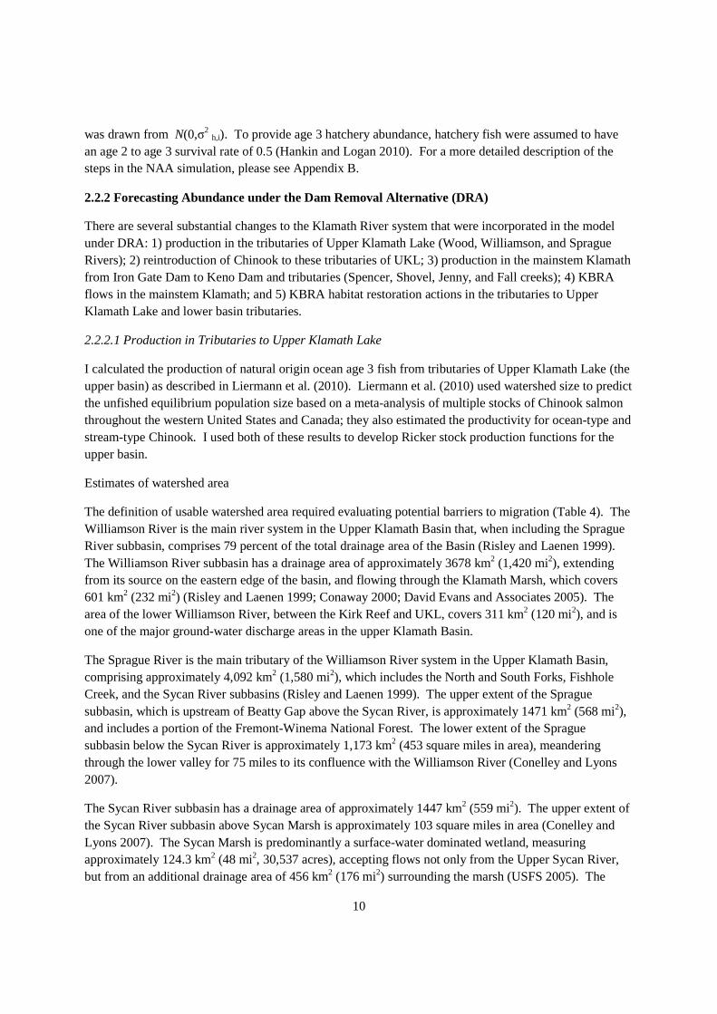
accuracy of draws from the target distribution, was calculated for each monitored quantity in the model. Monitored parameters in all models had SRF values that indicated samples were being drawn from the target distribution (i.e. SRF ) by 50,the stationary target distribution and were discarded produce approximately 1,000 draws from the stationcompute the posterior mean and 95% central probability intervals or credible intervals (95% CrI). The diagnostics were implemented using the R2WinBUGS package (Sturtz

I compared two models of stock recruitment; the first model was the bsecond alternative model with the common variability index (Equation 3). Criterion (DIC) to evaluate model predictive ability with a penalty for model complexity (Spiegelhalter et al. 2002).

where the deviance is equal to 2 deviance is a measure of model fit and decreases with better fitting models. The deviance is calculated at each iteration of the MCMC chain, and the first termmean of the deviance (e.g.,

equation 6 is pD, which is the effective number of parameters. number of parameters is typically less than the total number of estimated parameters, because information is being shared among random effects. The term 2002), and is the deviance evaluated at the posterior mean of the model param

).

2.1.5 Fisheries Reference Points

Reference points of the Ricker stock recruitment relationship were calculated using the following formula (Ricker 1975):

Smsy is the spawner that provides maximum sustainable yield. There is no analytical solution to the equation (Quinn and Deriso 1999), thus it was solved iteratively by maximizing the yield (is defined as

������� !"#$%+&���''''' (– ����

To calculate Smsy, I assumed the random effect of

Smax is the spawner abundance that provides maximum recruitment:

��)* =1

!

Sueq is the spawner abundance at adults. When the recruitment is defined as an earlier life stage, it is still useful as the spawner abundance that equals the abundance of the earlier life stage; here it is

�+,- . /012�3 /�

7

s from the target distribution, was calculated for each monitored quantity in the model. Monitored parameters in all models had SRF values that indicated samples were being drawn from the

) by 50,000 samples. The initial 30% of the samples were used to reach the stationary target distribution and were discarded (“burn in”) with the subsequent samples thi

000 draws from the stationary target distributions. The 1,posterior mean and 95% central probability intervals or credible intervals (95% CrI). The

diagnostics were implemented using the R2WinBUGS package (Sturtz et al. 2005) in R (RCDT 2010).

I compared two models of stock recruitment; the first model was the base model (Equation 2) and a second alternative model with the common variability index (Equation 3). I used Deviance Information Criterion (DIC) to evaluate model predictive ability with a penalty for model complexity (Spiegelhalter et

is equal to 2 the negative log likelihood (e.g., deviance is a measure of model fit and decreases with better fitting models. The deviance is calculated at each iteration of the MCMC chain, and the first term on the right hand side of the equation is the posterior

). The second term on the right hand side of the

, which is the effective number of parameters. In a hierarchical model the effective rs is typically less than the total number of estimated parameters, because information

is being shared among random effects. The term is defined as (Spiegelhalter et al. is the deviance evaluated at the posterior mean of the model param

2.1.5 Fisheries Reference Points

Reference points of the Ricker stock recruitment relationship were calculated using the following formula

is the spawner that provides maximum sustainable yield. There is no analytical solution to the equation (Quinn and Deriso 1999), thus it was solved iteratively by maximizing the yield (

, I assumed the random effect of CVI was at its average value (i.e,

is the spawner abundance that provides maximum recruitment:

undance at unfished equilibrium population size, assuming recruitment is defined as adults. When the recruitment is defined as an earlier life stage, it is still useful as the spawner abundance

the earlier life stage; here it is age 3 ocean fish.

s from the target distribution, was calculated for each monitored quantity in the model. Monitored parameters in all models had SRF values that indicated samples were being drawn from the

of the samples were used to reach with the subsequent samples thinned to

ary target distributions. The 1,000 draws were used to posterior mean and 95% central probability intervals or credible intervals (95% CrI). The

2005) in R (RCDT 2010).

ase model (Equation 2) and a I used Deviance Information

Criterion (DIC) to evaluate model predictive ability with a penalty for model complexity (Spiegelhalter et

(Equation 6)

). The deviance is a measure of model fit and decreases with better fitting models. The deviance is calculated at

on the right hand side of the equation is the posterior The second term on the right hand side of the

In a hierarchical model the effective rs is typically less than the total number of estimated parameters, because information

(Spiegelhalter et al. is the deviance evaluated at the posterior mean of the model parameters (e.g.,

Reference points of the Ricker stock recruitment relationship were calculated using the following formula

is the spawner that provides maximum sustainable yield. There is no analytical solution to the equation (Quinn and Deriso 1999), thus it was solved iteratively by maximizing the yield (R – S), which

(Equation 7)

was at its average value (i.e, CVI = 0)

(Equation 8)

population size, assuming recruitment is defined as adults. When the recruitment is defined as an earlier life stage, it is still useful as the spawner abundance

(Equation 9)

8

Estimating the model parameters in a Bayesian framework facilitated the calculation of the fishery reference points as probability distributions. Distributions for fishery reference points were calculated by drawing 1000 samples from the posterior distributions of the model parameters, calculating the reference point for each of the 1000 draws and forming a probability distribution.

2.1.6 Assumptions for retrospective analysis

The assumptions in conducting the retrospective analysis using the Ricker stock – recruitment model are the same as those enumerated in STT (2005, p. 2). In addition, I make the following assumptions in the retrospective stock recruitment analysis:

1. The flow metrics (July flow at Seiad on the Klamath River and July flow at Lewiston on the Trinity River) were representative of annual variability in flow. I evaluated multiple flow metrics in a correlation analysis to evaluate multiple flow metrics to residuals from the STT (2005) analysis (not shown). In addition, the amount of variability attributable to flow was relatively small compared to CVI; therefore, incorporation of alternative flow metrics should have a small effect on parameter estimates.

2. The Bayesian model is drawing samples from the stationary posterior distribution of model parameters (i.e., the model has converged). While there are tests for lack of convergence (i.e., SRF values) that were used here, there are no methods to guarantee convergence.

2.2 Forecasting Abundance under the NAA and the DRA

Under both the NAA and the DRA, the life cycle of Chinook was completed in two stages: 1) production of natural origin age 3 ocean fish from spawners and hatchery origin age 3 ocean fish from Iron Gate and Trinity River hatcheries, and 2) calculation of harvest, maturation rates, natural mortality, and escapement by the KHRM (Mohr In prep). The production of age 3 ocean fish was implemented with Monte Carlo simulations to incorporate uncertainty in the abundance forecasts. I conducted 1000 Monte Carlo simulations to characterize the uncertainty in future productivity under each of the two alternatives. Each iteration of the Monte Carlo simulation paired the NAA and DRA forecasts; parameter draws used in the production stage under NAA and DRA (e.g., values of CVIt) were the same under NAA and DRA for each iteration of the model. For example, the value of CVI2024 was the same in iteration 724 of NAA as in iteration 724 of DRA. Using the same covariate values in a given iteration allowed paired comparisons of model outputs, which were valuable for calculating the relative benefits of the two alternatives in spite of uncertainty in the absolute abundances.

I provide details on the production of age 3 ocean fish under the two alternatives below. The application of KHRM was the same between the NAA and DRA evaluations which also facilitated comparison of DRA and NAA on relative terms. In general, the default values of the KHRM were used in EDRRA. Values of the biological parameter set that were supplied for each run of KHRM were:

9

1) Na , which was a vector of abundances consisting of: age 3 hatchery and natural origin in the ocean, age 4 hatchery and natural origin in the ocean, and age 5 hatchery and natural origin in the ocean

2) ga, which was a vector of proportions of the natural origin consisting of: age 3 natural proportion, age 4 natural proportion, and age 5 natural proportion.

The KHRM operated as a deterministic harvest model with uncertainty in harvest and escapement arising only from the input of the Na , ga, vectors only. The fishery control rule defined the harvest rates based on expected levels of escapement in the absence of harvest (Mohr In prep), and under both the NAA and DRA the fishery control rule was an updated version of the amendment 16 fishery control rule (Appendix A). The default management parameters and the fishery parameters in the KHRM were not modified; therefore, the management and fishery behavior of the KHRM model was exactly the same under both alternatives.

The role of flow in the Klamath and Trinity Rivers was expected to affect hatchery survival rates, and flow was included in the forecasted production functions to age 3. Flows for the Klamath River at Seiad were forecasted for the 50 year period (2012 to 2061) as part of flow studies on the Klamath River in support of the Secretarial Determination process (Reclamation 2010). Two flow series were used as part of the hydrological evaluation of future conditions in the Klamath Basin; these were the flows under the Biological Opinion (NMFS 2010) and the flows as recommended under KBRA. In the Ricker stock recruitment model presented here, the flow covariate was normalized to have a mean value of 0 and a standard deviation of 1. In order to use the parameter values for flow (γIGH), hydrology data for the Klamath River at Seiad was normalized using the same values as the historical data (mean of 1589.0 cfs, sd = 944.17). These normalized flows are presented in Figure 2 to provide a comparison under the two alternatives. In the Trinity River, no such flow forecasts were available; therefore, I constructed a time series of flows that were consistent with historical flows. The constructed flow series for the Trinity was used for all iterations of EDRRA under NAA and DRA.

Monte Carlo simulation was used to integrate across the uncertainty in the model parameters with the objective of translating uncertainties in model inputs into uncertainties in model outputs (Manly 1997). Monte Carlo simulation is a technique that involves using random numbers sampled from some form of a probability distribution as input to a deterministic equation or model to derive an outcome under conditions of uncertainty. As the number of outcomes in the simulations approaches infinity, the statistics (mean, standard deviation, etc.) converge to their true value (Givens and Hoeting 2005).

2.2.1 Production to Age 3 in the Ocean under the No Action Alternative (NAA)

Forecasted production under the NAA consisted of production of natural origin and hatchery origin age 3 ocean salmon. Forecasts of natural production were based on the results of the retrospective Ricker stock-production function described previously (Equation 3). Values of CVIi,t were drawn for each iteration i and year t of the model, where t is now the year when the cohort is at age 3 and St-3 is the spawner abundance. The values for CVIi,t were drawn from a N(0,σ2 CVI,i ) and residual error εi,t from N(0, σ

2 ε,i). The values of the parameters of the stock production function (α’, β, δ) were drawn from their Bayesian posterior distributions. In each year the hatchery was operational, the Trinity River Hatchery produced 3 million and the Iron Gate Hatchery produced 6 million fingerlings. Values of log hatchery survival were drawn from their posterior distributions (e.g., κj, γj for j = IGH, TRH) and the residual error

10

was drawn from N(0,σ2 h,i). To provide age 3 hatchery abundance, hatchery fish were assumed to have an age 2 to age 3 survival rate of 0.5 (Hankin and Logan 2010). For a more detailed description of the steps in the NAA simulation, please see Appendix B.

2.2.2 Forecasting Abundance under the Dam Removal Alternative (DRA)

There are several substantial changes to the Klamath River system that were incorporated in the model under DRA: 1) production in the tributaries of Upper Klamath Lake (Wood, Williamson, and Sprague Rivers); 2) reintroduction of Chinook to these tributaries of UKL; 3) production in the mainstem Klamath from Iron Gate Dam to Keno Dam and tributaries (Spencer, Shovel, Jenny, and Fall creeks); 4) KBRA flows in the mainstem Klamath; and 5) KBRA habitat restoration actions in the tributaries to Upper Klamath Lake and lower basin tributaries.

2.2.2.1 Production in Tributaries to Upper Klamath Lake

I calculated the production of natural origin ocean age 3 fish from tributaries of Upper Klamath Lake (the upper basin) as described in Liermann et al. (2010). Liermann et al. (2010) used watershed size to predict the unfished equilibrium population size based on a meta-analysis of multiple stocks of Chinook salmon throughout the western United States and Canada; they also estimated the productivity for ocean-type and stream-type Chinook. I used both of these results to develop Ricker stock production functions for the upper basin.

Estimates of watershed area

The definition of usable watershed area required evaluating potential barriers to migration (Table 4). The Williamson River is the main river system in the Upper Klamath Basin that, when including the Sprague River subbasin, comprises 79 percent of the total drainage area of the Basin (Risley and Laenen 1999). The Williamson River subbasin has a drainage area of approximately 3678 km2 (1,420 mi2), extending from its source on the eastern edge of the basin, and flowing through the Klamath Marsh, which covers 601 km2 (232 mi2) (Risley and Laenen 1999; Conaway 2000; David Evans and Associates 2005). The area of the lower Williamson River, between the Kirk Reef and UKL, covers 311 km2 (120 mi2), and is one of the major ground-water discharge areas in the upper Klamath Basin.

The Sprague River is the main tributary of the Williamson River system in the Upper Klamath Basin, comprising approximately 4,092 km2 (1,580 mi2), which includes the North and South Forks, Fishhole Creek, and the Sycan River subbasins (Risley and Laenen 1999). The upper extent of the Sprague subbasin, which is upstream of Beatty Gap above the Sycan River, is approximately 1471 km2 (568 mi2), and includes a portion of the Fremont-Winema National Forest. The lower extent of the Sprague subbasin below the Sycan River is approximately 1,173 km2 (453 square miles in area), meandering through the lower valley for 75 miles to its confluence with the Williamson River (Conelley and Lyons 2007).

The Sycan River subbasin has a drainage area of approximately 1447 km2 (559 mi2). The upper extent of the Sycan River subbasin above Sycan Marsh is approximately 103 square miles in area (Conelley and Lyons 2007). The Sycan Marsh is predominantly a surface-water dominated wetland, measuring approximately 124.3 km2 (48 mi2, 30,537 acres), accepting flows not only from the Upper Sycan River, but from an additional drainage area of 456 km2 (176 mi2) surrounding the marsh (USFS 2005). The

11

lower extent of the Sycan River subbasin begins below the Sycan Marsh, and is approximately 601 km2 (232 mi2) in area (Conelley and Lyons 2007).

The Wood River subbasin is located in Klamath County, Oregon approximately 40 miles north of Klamath Falls. The subbasin has a drainage area of approximately 567 km2 (219 mi2) extending from the southern flanks of the Crater Lake highland within Crater Lake National Park and the Winema National Forest, and flowing southward through the Wood River Valley into Agency Lake (USBR 2005; Graham Matthews and Associates 2007).

The total estimate of watershed size for the tributaries to UKL was 4200.96 km2 (Table 4) Using samples from posterior distributions provided by Martin Liermann (Martin Liermann, NWFSC NOAA, March 28, 2011 personal communication) as described in Liermann et al. (2010), a stock production function was constructed for the tributaries to UKL. Liermann et al. (2010) used a version of the Ricker stock recruitment function defined in terms of the log productivity r and the unfished equilibrium population size E (the value where recruitment abundance equals spawning abundance). Liermann et al. (2010) found that the log productivity was different for ocean type and stream type Chinook; further, they found that the relationship between watershed size and E was different for ocean and stream Chinook.

Both stream and ocean type Chinook are expected to be present in the tributaries to UKL (Dunsmoor and Huntington 2006); therefore, the production functions for the tributaries to UKL incorporated productivity (r ) and unfished equilibrium population size (E) for a mixture of stream and ocean Chinook. To implement the mixture, the proportion of ocean and stream type were able to vary in each year. For each iteration i and year t of the model, a proportion of ocean Chinook pi,t was drawn at random from a Uniform(0,1) distribution.

The unfished equilibrium population size was calculated for stream type Chinook using Equation 8 of Liermann et al. (2010) (assuming L = 0 indicating stream Chinook), Enew stream. The unfished equilibrium population size was also calculated for ocean type Chinook using Equation 8 (assuming L = 1, indicating ocean Chinook), Enew ocean. The mixture of ocean and stream unfished equilibrium population size Enew, i t for iteration i and year t was calculated as follows:

56,7,9,� . ;9,�56,7 <=,)6,9 + 21 − ;9,�356,7 �@A96B,9 Equation (11)

In a similar fashion, the values of productivity rnew, i,t were formed as a mixture of ocean and stream type r values from Liermann et al. (2010).

C6,7 ,9,� . ;9,�C6,7 <=,)6,9 + 21 − ;9,�3C6,7 �@A96B,9 Equation (12)

The values of 56,7,9,� , C6,7 ,9,�, and the spawner abundance three years previously (Si,t-3) allowed the calculation of upper basin adult recruits in the absence of fishing via Equation 1 in Liermann et al. (2010). In addition, annual variability in recruitment was modeled with a random effect wi,t. The random effect for annual variability in the tributaries of UKL was the same as the lower basin�9 CVI i, t-2. Finally the recruitment calculated to the adult returning stage was converted from adult to 3 year ocean fish (via the N(2.03, 0.01) expansion factor ) .

2.2.2.2 Modeling the reintroduction to tributaries of Upper Klamath Lake

12

The reintroduction of Chinook to the tributaries of UKL was assumed to start in 2019 with fry being planted in the tributaries to UKL prior to dam removal in 2020. The reintroduction process is expected to construct a conservation hatchery that is capable of seeding the tributaries to UKL with fry to capacity (Hooton and Smith 2008). There is no fry or other juvenile freshwater stage in the model; therefore, stocking to capacity was modeled by assuming that the numbers of adult returns were at or above the unfished equilibrium population size 56,7,9,� from 2019 to 2029 for model iteration i and year t.

2.2.2.3 Production from Iron Gate to Keno Dam

From Iron Gate Dam to Keno Dam, the mainstem and tributaries to the mainstem (Spencer, Shovel, Jenny, and Fall creeks) watershed area was estimated at 1792.2 km2 (Lindley and Davis In prep). Posterior samples from the distributions for parameters defining the relationship between watershed size and unfished equilibrium population size E were used to construct the posterior predictive distribution for Enew given the watershed size for Iron Gate to Keno Dam using Liermann et al. (2010) and assuming ocean type Chinook.

Further, the following steps were taken to modify the Ricker stock recruitment relationship under NAA to include the additional spawning area below Keno Dam in the DRA:

1. Calculate the distribution of unfished equilibrium population size for the Iron Gate to Keno mainstem and tributaries using Equation 8 of Liermann et al. (2010) assuming a watershed size of 1792.2 km2 and ocean Chinook, EKeno:IG

2. Multiply the unfished equilibrium population size for adult recruits by the adult recruit to age 3 ocean factor CF

3. Use the distribution of Sueq calculated in Equation 9 of this document for the pre-dam removal estimate of unfished equilibrium population size (recruitment defined as age 3 ocean abundance).

4. Add the unfished equilibrium abundance for habitat from Keno to Iron Gate calculated in step 1 to the old equilibrium abundance from step 2 to calculate Sueq new

5. Calculate a new distribution for the β parameter with the additional capacityby re-arranging Equation 9

�6,7 . DE"FGH IGJ Equation (10)

Because there were 1000 posterior samples for each of these quantities (EKeno:IG and Sueq ) the above calculations were carried out 1000 times for each iteration i of the model . The 1000 samples of the distribution of βnew were used for the forecasting the productivity of the Klamath River below Keno Dam after 2020 (i.e., replace β in Equation 10 with �6,7).

2.2.2.4 Modeling the effects of KBRA

Since the Fisheries Restoration Plan under KBRA has yet to be developed, specific restoration projects within each of the tributary streams currently included in the model have yet to be identified. Habitat restoration actions were specifically identified for the three major lower basin tributary streams (Scott, Shasta, and Salmon) and in the tributaries to Upper Klamath Lake. I assumed that for the purposes of this model, all of the habitat restoration actions identified will have benefits beginning in 2013 and accruing through 2061.

13

Stakeholders identified the likelihood that annual variability in recruitment from the tributaries to UKL could vary with Klamath River flows. The variation in production due to flow variability is not known given the lack of information on the upper basin, however. I assumed that flow variability affected outmigrating UKL fish to a similar degree as the IGH hatchery fish. Thus, the posterior distribution on γIGH was used as a posterior predictive distribution on the effect of flow on production in the tributaries to UKL. The values of the flows at Seiad used in the retrospective analysis were normalized to have a mean of 0 and a standard deviation of 1; therefore, the KBRA flows used to compute annual variability in recruitment to age 3 form tributaries to UKL under DRA were transformed using the same mean and standard deviation as the Seiad series.

Stakeholders have also identified the likelihood that KBRA actions will increase productivity between 2012 and 2061. The uncertainty in productivity was characterized by the posterior distribution of �K; thus, the posterior distribution of �K provides a description of the range of possible productivity values in the lower basin along with the probability of observing those values (by definition of a posterior probability distribution). I implemented the improvement in productivity due to KBRA actions in EDRRA by drawing samples from a truncated distribution of productivity. By using a truncated distribution, the upper range of productivity values did not change, whereas the lower values of productivity became less likely over time. In Figure 3, the process of drawing posterior predictive samples from truncated distributions is depicted. Early in the time series, low as well as high productivity values can be drawn from the distribution; however, as the time series progresses lower values of productivity are rejected and a new draw must be made until one from the Accepted region is obtained. In practice, the draws were made from truncated Normal distributions via the package msm (Jackson 2011) in the statistical programming language R (RCDT 2010). The lower threshold value was set at the 0 quantile in 2012 (i.e., the full distribution was sampled) and the quantile increased linearly to 0.25 by 2061; that is, by 2061 only the upper 0.75 portion of the distribution could be sampled (lower threshold at quantile of 0.25). Draws from the truncated distribution are distinguished by an asterisk on the parameter.

For example, truncated draws from the lower basin productivity �Kare distinguished as �′∗

A similar approach was implemented for the tributaries to UKL, where uncertainty was characterized through the use of posterior predictive distributions of productivity for ocean type and stream type Chinook presented in Liermann et al. (2010) (i.e, rnewocean and rnewstream). The lower threshold for sampling in 2012 was set at the 0 quartile (the entire distribution could be sampled) and moved linearly to the 0.25 quantile by 2061 (truncated to the upper 0.75 portion of the distribution). The mixture of ocean and stream Chinook was then applied via the proportion of ocean Chinook pi,t after the draws from the truncated distributions of rnewocean and rnewstream.

In a similar fashion, the values of productivity rnew, i,t were formed as a mixture of ocean and stream type r values from Liermann et al. (2010).

C 6,7 ,9,�∗ . ;9,�C6,7 <=,)6,9∗ + �1 − ;9,��C6,7 �@A96B,9∗ Equation (13)

Please see Appendix B for the specific steps of production of Age 3 Chinook under DRA.

2.2.3 Assumptions to forecasting under DRA and NAA

Multiple assumptions were made to forecast abundance under DRA and NAA:

14

1. Data used for the stock-recruit analysis and subsequent simulation modeling were based on current and past conditions and are also indicative of future conditions in the Lower Klamath Basin

2. Stock recruitment relationships developed from the retrospective analysis will be the same in the future. Any modifications to the stock recruitment relationships for the Lower Klamath Basin in the future will only occur as modeled (e.g., KBRA effects under DRA).

3. Annual variability in stock recruitment in the lower basin will be of a similar magnitude to past annual variability in stock recruitment.

4. The use of Liermann et al. (2010) work assumes that the Klamath system falls within the range of watersheds evaluated in their analysis. The Liermann et al. (2010) work was used due to its incorporation of a broad range of watersheds, inclusion of stream and ocean type Chinook. and the explicit incorporation of uncertainty in predictions for new streams. The EDRRA model assumes that production from the Klamath River at the beginning of the time series could range from the worst to the best rivers analyzed in Liermann et al (2010).

5. Conversion from adult abundance to age 3 abundance is valid based on data presented in STT (2005) (Table 1).

6. Capacity for the Iron Gate to Keno reach calculated using Liermann et al. (2010) can be added to capacity below Iron Gate estimated via the retrospective stock recruitment analysis.

7. Chinook in the Lower Basin below Keno will be predominantly ocean type. 8. Chinook in the Upper Basin above Keno will be a mixture of ocean and stream type; the relative

proportion of each type will vary annually. 9. The Sycan Marsh on the Sycan River and the Klamath Marsh on the Williamson River are

barriers to Chinook migration. 10. Implementation of KBRA in the EDRRA model assumes that the conditions in the Klamath River

will improve over the 50 year time period of the model. This process was modeled by removing the chance for low productivity in later years of the time series. In future years, the likelihood that the Klamath would act like the worst rivers in Liermann et al. (2010) diminishes.

11. Annual variability in production of age 3 ocean recruits will be highly correlated in the upper and lower basin.

12. Flow variability in the Klamath River will affect production of Chinook in the upper basin to a similar degree as it affected survival of IGH hatchery fish. Namely, the posterior distribution on γIGH was used as a posterior predictive distribution on the effect of flow on the production in the tributaries to UKL.

13. Under the active reintroduction of the upper basin, production assumes adult abundances at or above the unfished equilibrium population size for the period 2019-2029.

14. Default values provided in the KHRM (described in Mohr et al. In prep.) for maturation rates, ocean survival rates, etc. were appropriate for future Klamath Basin Chinook stocks.

15. The fishery management is the same for DRA and NAA (please see Appendix A). Further, it is fixed for the time period of the model simulations.

16. The fishery is managed with perfect information; that is, fishery managers have perfect information of the abundances at each age and the proportion of hatchery fish in each age.

17. The fishery operates perfectly; that is, the allocated catch from the fishery managers is caught to meet the target harvest and escapement levels.

15

3 Results

3.1 Retrospective Analysis

The Ricker stock-recruitment function with the index of common variation (CVI) provided a better explanation of the variability in the age 3 ocean recruitment (DIC = 662.8, pD = 25.3, mean deviance = 637.5) than the base model (DIC = 683.4, pD = 28.5, mean deviance = 654.9). The difference in DIC values was approximately 20 units, which is strongly supportive of the alternative model (Spiegelhalter et al. 2002). The difference in DIC values was due primarily to a decrease in mean deviance in the model, indicating an improvement in the prediction of age 3 ocean abundance by including the CVI as a covariate. Scale reduction factors indicated that samples were occurring from a stationary distribution in both models (i.e., values were near 1 for parameter estimates in both models). Observed versus predicted plots under the alternative model indicated that predicted median ocean age 3 abundances were indicative of observed abundances, but as may be expected with fitting spawner-recruit relationships (e.g., Hilborn and Walters 1992), some additional variability remained to be explained (Figure 4).

The CVI was estimated by capturing annual variability in hatchery survival common to both the IGH and TRH fingerling release groups (Figure 5). Much of the annual variability in survival of IGH and TRH releases was due to the common source of variability between the two hatcheries (Figure 6), with some remaining variability due to hatchery specific factors. Estimates of the standard deviation of the CVI provide an indicator of the magnitude of the effect on hatchery survival. For example, TRH survival rates could vary from 4.8% to 0.38% for a 1 standard deviation increase and a 1 standard deviation decrease in the value of CVI, respectively.

Mean survival to age 2 was higher for TRH releases (1.35%) than IGH releases (0.9%) (values obtained by transforming mean values of κ in Table 5). Summer flows in the Trinity River in July at Lewiston were positively related to annual variability in survival of TRH releases; the posterior distribution of γTRH had a mean value of 0.3 (95% CrI: -0.038, 0.613, Table 5). Although the 95% CrI included zero, there was a 0.963 probability that flow was positively related to hatchery survival. Summer flows in the Klamath River (July flows at Seiad) were positively related to variability in IGH releases. The posterior distribution of γIGH was positive and the 95% CrI did not include 0 (Table 5); the probability of higher flows having a positive relationship with IGH survival in the Klamath River was > 0.999.

The common variability index (CVI) was variable among years and matched the pattern in log hatchery survival rates (Figure 6). While the pattern in the CVI may be informative, it is not known whether the magnitude of annual deviations is the same for natural recruitment to the age 3 ocean stage. A parameter was included in the model to allow the variability from the hatchery fish (CVI) to be scaled to the natural recruitment via δ. The inclusion of the δ parameter also allowed the stock recruitment function to ignore the CVI (e.g., if the δ value was 0). Median posterior estimates of δ were 0.61 (95%CrI: 0.32, 0.93) indicating that there was a positive relationship between recruitment variability and CVI, i.e., years with higher survival of TRH and IGH fingerlings were concurrent with positive deviations from the mean stock recruitment relationship.

16

The result of the retrospective model was a stock production function that could be used to forecast the levels of production with uncertainty for the Klamath basin below Iron Gate Dam in the No Action Alternative. The uncertainty in the stock production function is substantial, even in the absence of the CVI effect (i.e., assuming CVI = 0) (Figure 7). The fishery reference points indicate the levels of uncertainty in the stock recruitment relationships (Table 6). The spawning abundance that maximizes yield is approximately 48,000 spawners (95%CrI: 34,924, 86,141). The level of spawner abundance that maximizes recruitment has a median of 58,360 (95%CrI: 39,325, 109,167), whereas the median spawner abundance that equals the abundance of 3 years old in the ocean was estimated at 143,660 (106,407; 232,915).

The Liermann et al. (2010) model was also calculated for the lower basin assuming a watershed area of 9,653 km2 (assuming a total watershed area of 12,066 km2 for the Salmon, Shasta, Scott, Lower & Upper Klamath below Iron Gate and removing 20% due to watershed area draining directly into anadromous streams, D. Chow, NMFS, pers. comm.). This was completed to provide a point of comparison between the Liermann et al. (2010) approach and existing estimates of Smsy in the lower basin. The Liermann et al. (2010) median estimates of Smsy assuming a 9.653 km2 watershed was 43,360 (95%CrI: 17.905, 95,500). In comparison, STT (2005) estimated Smsy to the adult stage as 40,700 (95% confidence interval: 32,200, 54,100). This result suggests relatively good agreement between Liermann and the STT (2005) analysis.

3.2 Spawner recruitment functions for DRA

3.2.1 Lower Klamath Basin

Under DRA the spawning habitat was increased by 1790 km2, which equated to an adult unfished equilibrium population size of 23,613 (95% CrI: 11,063.1; 47,625.1) (Liermann et al. 2010). The adults were expanded into age 3 ocean recruits, which lead to redefining the capacity parameter in the Ricker stock recruitment relationship. The stock recruitment relationship in the lower basin shifted due to the added capacity in 2020 (Figure 8). As a result, the fishery reference points shifted to higher median levels (Table 7) with the median Smsy of 63,838 under DRA as compared to 48,475 under NAA and median Smax of 79,623 under DRA versus 58,361 under NAA. These results were computed in the absence of KBRA to provide estimates of changes in the stock production function early in the time series.

The stock production function in the lower basin shifted over the time series due to KBRA actions affecting productivity in the lower basin tributaries (Stillwater Sciences 2010). The stock production function in 2012 was thus different than in 2061 due to the portion of the posterior distribution of α’ that was sampled (Figure 9). As a result, the stock recruitment relationship shifted over the time series such that median recruitment was higher in 2055 relative to 2025, although uncertainty in recruitment remained largely unchanged (Figure 10).

3.2.2 Tributaries to Upper Klamath Lake

The stock production function in the upper basin was derived from assuming mixed stream and ocean Chinook life history types and sampling log productivities from posterior predictive distributions provided in Liermann et al. (2010). The median log productivity from assuming the mixed life history rnew was 1.69 (95%CrI: 1.14; 2.24). The median estimate of unfished equilibrium population size for the tributaries to UKL using the results of Liermann et al. (2010) was 17,232 (95%CrI: 8,330; 30,439) for

17

stream type and 53,691 (95%CrI: 23,598; 98,891) for ocean type Chinook, whereas the mixed ocean and stream type estimate was 34,350 (95%CrI: 12,964; 73,304). Restoration work in the tributaries to UKL was assumed to alter the distribution of rnew

between 2012 and 2061 such that lower values of log productivity became less likely over this period (rnew

*) (Figure 11). As a result, the stock recruitment relationship (defined from spawner to age 3 in the ocean) in 2055 had higher recruitment of age 3 ocean Chinook for a given spawner abundances when compared to the stock recruitment relationship in 2025 (Figure 12). The difference between the 2025 and the 2055 stock recruitment relationships was most pronounced at spawner abundances less than approximately 33,000.

3.3 Comparison of Alternatives

To support the decision process, the relative benefits of performing one action over another in the face of parametric and environmental uncertainty were calculated. Because the model iterations were paired (i.e., the same values of CVIi,t , the same value of δi, the same value of ui,j,t , etc. for hatchery j, iteration i in year t in NAA as in DRA), the probability that DRA was greater than NAA could be calculated (i.e., the number of model iterations in which DRA was greater than NAA). If there is no benefit to one action over the other, the probability will be 0.5 (i.e., 50:50 chance of higher abundance); however, if the probability is consistently greater than 0.5, then there is support for DRA despite uncertainty in the absolute abundance forecast.

I also calculated the percentage increase in abundance for each paired iteration as (DRA – NAA)/NAA * 100%, which provided a quantitative estimate of the difference in abundance. There were three periods that could have different relative levels of abundance under DRA versus NAA: the period between model initiation and dam removal (2012- 2020); the period after dam removal but with active reintroduction in the tributaries to UKL (2021-2032); and the final period when the population in the tributaries to UKL are assumed to be established and Iron Gate Hatchery production has ceased (2032-2061).

Escapement in the absence of fishing was calculated by the KHRM prior to determining the harvest rate, and it provided an estimate of total escapement to the Klamath Basin. The probability that forecasted escapement in the absence of fishing is higher under DRA than NAA between 2012 and 2020 is 0.54 (median of the annual probabilities from 2012-2032) (Figure 13). The probability is 0.79 from 2021- 2032 and 0.78 from 2033 to 2061 that forecasted escapement under DRA was higher than NAA (Figure 13). The percentage increases in escapement of DRA relative to NAA in these three periods were 10.8% (2012-2020), 81.8% (2021-2032) and 81.4% (2033-2061) (Table 8).

Escapement to the Lower Klamath Basin was marginally higher under DRA than NAA (Figure 14). The probability that forecasted escapement to the Lower Klamath basin under DRA was greater than NAA was 0.50 between 2012 and 2020. The probability of DRA being greater than NAA was 0.54 and 0.56 for the periods 2021-2032 and 2033-2061, respectively (Figure 14). Over these three periods, the median percentage increases in escapement to the lower basin in DRA relative to NAA were approximately 7% to 9% after 2021 (Table 8).

Due to the structure of the KHRM, ocean recreational and ocean commercial harvest had the same relative response of DRA versus NAA (Figure 15 and 16). The probability of increased ocean harvest from 2012 to 2020 was 0.54. The improvement above 50% during the early period was due to KBRA restoration actions. After dam removal and during active reintroduction (2021-2032), the probability that

18

ocean harvest was greater in DRA than NAA was 0.79. The probability of higher harvest dropped slightly to 0.72 with the cessation of active reintroduction and the loss of Iron Gate Hatchery production after 2032 (Figures 15 and 16). Median estimates of the percentage increase in ocean harvest due to DRA was approximately 9% from 2012 to 2020, rising to 63% from 2021 to 2032, and dropping to 46.5% after 2033 (Figure 15 and 16, Table 8).

Patterns in river harvest were similar to those for lower basin escapement, with relatively small increases in river harvest under DRA versus NAA (Figure 17). Prior to 2020, river harvest was roughly equivalent for NAA and DRA. The probability that DRA was greater than NAA was 0.48 prior to dam removal in 2020 (but equal to 0.5 if one includes the iterations where DRA equals NAA). After dam removal, the probability of increases in river harvest under DRA was consistent at 0.62. The pattern in river harvest was due to a 25,000 limit on capacity of recreational fishers (Mohr In prep), which minimized the amount that the DRA and NAA runs could differ. As a result, the median percentage increases in DRA relative to NAA runs were 0% during the early period (2012-2020) and increased to approximately 9% after dam removal (Table 8).

Tribal harvest was similar in pattern to ocean harvest (Figure 18), which reflected the fishery allocation rules incorporated into the KHRM. The probability of tribal harvest increasing under DRA was 0.54 prior to 2020, increasing to 0.79 during the active reintroduction period (2021-2032) and dropping down to 0.72 afterwards (Figure 18). Median estimates of the percentage increase in tribal harvest was roughly 10% before 2020, climbing to 71.5% during 2021-2032, and dropping to 54.8% thereafter.

4.0 Discussion

The forecasted levels of escapement and harvest are determined by KHRM; therefore, understanding how KHRM operates provides some insight into the relative levels of escapement and harvest forecasted under NAA and DRA. The main driver of the KHRM behavior is the F- control rule, and the rule used in the forecasts under NAA and DRA is an updated amendment 16 rule (Appendix A). This rule is based on an optimal (i.e., escapement that produces maximum sustainable yield) escapement target after harvest of 40,700 (STT 2005). The updated F-control rule was developed to maximize yield under the current conditions (i.e., NAA), but it may not be optimal for DRA. The application of the updated rule to DRA affects the results here in two ways. First, given the additional recruitment to the fishery that arises from production in the Keno to Iron Gate reach and tributaries to UKL, the escapement and harvest forecasted under DRA were likely not managed optimally. Higher harvest and escapement (and potentially more consistent harvest and escapement) may be attainable by specifying an F-control rule optimized for the spawner recruitment relationships under DRA. Second, the probability of fishery closure was determined by F control rule and its escapement floor. There may be a trade-off between higher probability of closures and higher harvest rates that would need to be explored based on the spawner recruitment relationships for the lower and upper basins. Ultimately, any modification of the F-control rule would occur through a formal process under the Pacific Fishery Management Council, and modeling this process was well beyond the scope of this effort.

The KHRM was implemented in EDRRA with simplifying assumptions to highlight differences in the production under NAA and DRA. These assumptions affected the absolute estimates of harvest, and

19

attempts to compare the harvest under NAA to historical catches may be misleading. Catch in the ocean and river fisheries between the mid 1990’s through 2010 had a median value of 33,725 (PFMC 2011). Median forecasts of harvest under NAA presented here are well above the historical catches for at least two reasons. First, the ocean abundance supplied to the KHRM here is known without error; in other words, there is no error between the abundance in the preseason forecast and the postseason estimate. In reality, the level of error in preseason to postseason is not trivial, and the ratio of preseason forecast/postseason estimate of age 3 Klamath River fall Chinook has ranged from an overestimate of 2.5 to an underestimate of 0.34 in the period 1991 to 2010 (Table II-3 in PFMC 2011). As a result, the fishery management process used here was able to prescribe the exact numbers of fish to be harvested to reach the escapement objective. Second, the fishery described here operates perfectly; therefore the numbers of fish prescribed to be captured to meet the escapement objective are actually captured with perfect accuracy. The result of these two simplifying assumptions of the management and the fishery are that the escapement returning to spawn is close to 40,700 in most years (median of 42K under NAA) which means that the stock is close to Smsy under NAA and producing optimally.

I estimated a spawner recruitment relationship from spawners to age 3 ocean fish using historical data on the Klamath Basin that was similar in many respects to STT (2005). Although the recruitment was defined to different locations in the life history (to age 3 in the ocean here, whereas STT (2005) defined recruitment as adult escapement), the fishery reference points Smsy and Smax can be compared. The bias adjusted mean estimate of Smsy calculated in STT (2005) was 40,700 (95% confidence interval [CI]: 32,200; 54,100) and the bias adjusted mean estimate of Smax was 56,900 (95%CI: 42,400; 84,200). The reference points estimated in the Bayesian analysis here (Table 6) were higher with broader 95% credible intervals relative to the 95% confidence intervals in STT (2005). In particular, the median estimate of Smsy was 48,475 in the Bayesian analysis was higher than the bias adjusted mean estimate of 40,700 (STT 2005). If the distributions were the same, the median would be expected to be below the bias adjusted mean due to the shape of the lognormal distribution. Thus although the bias adjusted mean of Smax in STT (2005) and the Bayesian analysis are similar, the level of Smax implied by the Bayesian analysis was larger than in STT (2005). It is not surprising that the levels of Smsy and Smax differ between the two approaches. First, the estimation of the stock recruitment relationship to an earlier life stage in the Bayesian analysis (age 3 in the ocean) will affect the estimates of log productivity. Second, the annual variability in productivity was characterized differently in the Bayesian analysis than in STT (2005) which also affected log productivity estimates. Reference points that use the estimated log productivity (e.g., Smsy) will be affected by the difference in log productivity estimates.

Finally, one advantage of the Bayesian analysis is the incorporation of parameter uncertainty into the estimation approach as probability distributions (Gelman et al. 2004). Derived quantities of the model can then be computed as probability distributions by integrating over the uncertainty in the parameters. The full posterior distribution on the derived quantity can then be evaluated for inference (e.g., McAllister et al. 1994, Punt and Hilborn 1997, Liermann et al. 2010). Analyses of similar data sets under Bayesian and frequentist approaches may result in different results depending upon the marginal likelihood of the coefficient estimate. When the information in the data on a particular parameter value are informative, the difference between Bayesian and frequentist inference will be small; however, when the information on the parameter is limited (e.g., for parameters such as Smax = β-1 estimated from spawner recruitment data), the differences between the two approaches are likely to be greater. For this reason, comparison of approaches under Bayesian and frequentist approaches may provide different inference, and almost

20

always indicate greater uncertainty in the value of the derived quantities in the Bayesian analysis (Gelman et al. 2004, Congdon 2002).

In the process of developing the tools for evaluating NAA and DRA, I computed estimates of equilibrium population sizes for the tributaries to UKL and the reach from Iron Gate Dam to Keno Dam. The median estimates of unfished equilibrium population size using the Liermann et al. (2010) posterior distributions was approximately 23,000 ocean type Chinook in the Keno to Iron Gate reach and approximately 35,000 stream and ocean type Chinook in the tributaries to UKL. There are several other estimates of equilibrium unfished or fished population sizes for both the tributaries to UKL and the Iron Gate to Keno reach that can be used to put the estimates computed here into context. Most recently, Lindley and Davis (In prep) estimated an equilibrium fished population size of 720 for the Keno to Iron Gate reach and an estimate of 2372 for the tributaries of UKL (Wood, Williamson, and Sprague Rivers). Further they compare their estimates to calculations of equilibrium unfished population abundances in Liermann et al. (2010) using assumptions consistent with their model. The assumptions in Lindley and Davis (In prep) differ than those made here with respect to accessibility to portions of the watershed and the spatial structure of Chinook populations once they become established; therefore calculations using parameters in Liermann et al (2010) are not directly comparable between the two works. Finally, Dunsmoor and Huntington (2006) developed a tabular summary of aquatic habitat conditions in the Upper Klamath Basin with particular emphasis on areas above UKL. They estimated that current habitat conditions above Iron Gate Dam could support approximately 14,864 spawning fall Chinook salmon and 32,706 spawning spring Chinook salmon. Huntington (2006) developed estimates of adult Chinook to the Klamath Basin upstream of IGD using five different methods and estimated between 9,180-32,040 Chinook. These estimates are roughly comparable to the 10,000 to 50,000 levels of Chinook escapement upstream of Iron Gate Dam calculated under EDRRA.

Ultimately, the specifics of how anadromy would be restored to the Klamath Basin will require additional planning, and there are many details that were excluded from this analysis by necessity. There are several factors that have been discussed as potentially modifying the degree to which anadromy may be restored to the Upper Klamath Basin. Water quality in UKL can be problematic for salmonids with summer temperatures exceeding 25 C and dissolved oxygen levels at 4mg/L or below during the summer (Wood et al. 2006). Thus, the conditions in UKL may be a factor in determining the type of life – history strategies that are successful due to acceptable windows into and out of the tributaries to UKL. Ceratomixta shasta currently affects natural origin juveniles migrating through the mainstem Klamath River. The prevalence of the disease appears to be tied to the density of the polychaete host and the flow and temperature conditions under which juveniles may be exposed to the parasite (Bartholomew and Foott 2010). The parasite C. shasta is also located in the Williamson River (Bartholomew and Foott 2010), although the strain there is not virulent to Chinook. It is not known whether the strain that is virulent toChinook will become established in the tributaries to UKL and affect the production potential of those tributaries.

Still, recent studies suggest that with the provision of suitable passage facilities at downstream dams or dam removal, Chinook salmon could be re-introduced and restored to waters in the Upper Klamath Basin (Dunsmoor and Huntington 2006; Hooton and Smith 2008; Butler et al. 2010); further, substantial historical evidence shows that both Chinook salmon and steelhead trout historically used the streams of the Upper Klamath Basin for spawning and for juvenile rearing (Hamilton et al. 2005; Fortune et al.

21

1966). Finally, NMFS and USFWS required anadromous fish passage as a condition for issuing a Federal Energy Regulatory Commission (FERC) license to operate the dams; thus, restoration of anadromy to the upper Klamath Basin will be an important part of the FERC relicensing process.

22

5 References

Andersson, J.C.M. 2003. Life history, status and distribution of Klamath River Chinook Salmon. Department of Geology, University of California, Davis, CA, USA.

Bartholomew, J.L., and J.S. Foott. 2010 (draft). Compilation of information relating to Myxozoan Disease effects to inform the Klamath Basin Restoration Agreement. Oregon State University and U.S. Fish and Wildlife Service. 53 pp.

Berger, James. 2006. Statistical Decision Theory and Bayesian Analysis. Second Edition. Springer. New York, NY, USA.

Box, G.E.P and G.C. Taio. 1973. Bayesian Inference in Statistical Analysis. Addison-Wesley, New York, NY, USA. 532.

Butler, V. L., J. A. Miller, D. Y. Yang, C. F. Speller, N. Misarti. 2010. The Use of Archaeological Fish Remains to Establish Pre-development Salmonid Biogeography in the Upper Klamath Basin. Prepared for National Marine Fisheries Service by Portland State University Department of Anthropology. 101 pp.

California Department of Fish and Game (CDFG). 2011. (Megatable) Klamath basin fall Chinook salmon harvest, escapement, and run-size estimates, 1978-2010.

Clemen, Robert. 1996. Making Hard Decisions. 2nd Edition. Duxbury Press. Pacific Grove, CA, USA.

Conaway, J. S. 2000. Hydrogeology and Paleohydrology in the Williamson River Basin, Klamath County, Oregon. Master’s thesis. Portland State University. Available at: http://nwdata.geol.pdx.edu/Thesis/FullText/2000/Conaway/

Congdon, P. 2002. Bayesian Statistical Modeling. John Wiley and Sons. New York, NY, USA.

Connelly, M. and L. Lyons. 2007. Upper Sprague Watershed Assessment. Prepared for: Klamath Basin Ecosystem Foundation, Klamath Falls, OR. Available at: http://www.klamathpartnership.org/watershed/upsprag/index.shtml

David Evans and Associates (DEA). 2005a. Upper Williamson River Watershed Assessment. Prepared for Klamath Ecosystem Foundation, Upper Williamson River Catchment Group, in cooperation with the Upper Klamath Basin Working Group and the Klamath Watershed Council. Available at: http://www.klamathpartnership.org/watershed/upwill/index.shtml

David Evans and Associates (DEA). 2000. Williamson River Delta Restoration Project Environmental Assessment. Prepared for the U.S. Department of Agriculture/Natural Resources Conservation Service In Partnership with The Nature Conservancy. Available at: http://klamathwaterlib.oit.edu/cdm4/item_viewer.php?CISOROOT=/kwl&CISOPTR=490&CISOBOX=1&REC=14

23

Dunsmoor and Huntington. 2006. Suitability of Environmental Conditions within Upper Klamath Lake and the Migratory Corridor Downstream for Use by Anadromous Salmonids Technical Memorandum for the Klamath Tribes. 80 pages.

Fortune, J.D., A.R. Gerlach and C.J. Hanel. 1966. A study to determine the feasibility of establishing salmon and steelhead in the Upper Klamath Basin. Oregon State Game Commission and Pacific Power and Light Company, Portland, Oregon.

Gannett, M. W., K. E. Lite, Jr., J. L. La Marche, B. J. Fisher, and D. J. Polette. 2007. Ground-water hydrology of the upper Klamath Basin, Oregon and California: U.S. Geological Survey Scientific Investigations Report 2007-5050, 84 p. Available at: http://pubs.usgs.gov/sir/2007/5050/pdf/sir20075050.pdf

Gelman, A., J. Carlin, H.S. Stern, and D.B. Rubin. 2004. Bayesian Data Analysis. CRC Press. 551.

Gilks, W. and D. Spiegelhalter. 1996. Markov chain Monte Carlo in practice. Chapman & Hall/CRC. 552.

Givens, G. and J.A. Hoeting. 2005. Computational Statistics. John Wiley and Sons, Hoboken, New Jersey, USA.

Graham Matthews and Associates. 2007. Draft WY 2006 Project Monitoring Report. Volume 1: Surface water. Prepared for Klamath Basin Rangeland Trust, Ashland, Oregon.

Hamilton, J.B., G.L. Curtis, S.M. Snedaker, and D.K. White. 2005. Distribution of anadromous salmonids in the Upper Klamath River Watershed prior to hydropower dams, a synthesis of the historical evidence. Fisheries 30(4): 10-18.

Hamilton, J., M. Hampton, R. Quinones, D. Rondorf, J. Simondet, and T. Smith. 2010. Synthesis of the effects of two management scenarios for the Secretarial Determination on removal of the lower four dams on the Klamath River, Final Draft dated November 23, 2010.

Hankin, D.G. and E. Logan. 2010. A Preliminary Analysis of Chinook Salmon Coded-Wire Tag Recovery Data from Iron Gate, Trinity River, and Cole Rivers Hatcheries, Brood-Years 1978 – 2004. Prepared by the Humboldt State University Sponsored Programs Foundation

Hilborn, R. and C.J. Walters. 1992. Quantitative Fisheries Stock Assessment: Choice, Dynamics, and Uncertainty. Chapman and Hall, New York, NY. USA.

Hooton, B. and R. Smith. 2008. A Plan for the Reintroduction of Anadromous Fish in the Upper Klamath Basin. Oregon Department of Fish and Wildlife. March 2008.

Huntington, C.W. 2006. Estimates of anadromous fish runs above the site of Iron Gate Dam. Technical memorandum to the Klamath Tribes, Chiloquin, Oregon. Clearwater BioStudies, Inc., Canby, Oregon. 15 January 2006.

24

Jackson, Christopher. 2011. Multi-State Models for Panel Data: The msm Package for R. Journal of Statistical Software, 28(8), 1-29. url http://www.jstatsoft.org/v38/i08/.

Lane and Lane Associates. 1981. The Copco Dams and the fisheries of the Klamath Tribe. U.S. Department of the Interior, Bureau of Indian Affairs, Portland, OR. Available at: http://www.fws.gov/yreka/HydroDocs/Lane-and-Lane-1981.pdf

Liermann, M., R. Sharma, C. Parken. 2010. Using accessible watershed size to predict management parameters for Chinook salmon, Oncorhynchus tshawytscha, populations with little or no spawner-recruit data: a Bayesian hierarchical modelling approach. Fisheries Management and Ecology 17: 40-51.

Lindley, S. T and H. Davis. In preparation. Using model selection and model averaging to predict the response of Chinook salmon to dam removal. National Marine Fisheries Service (NMFS), Southwest Fisheries Science Center (SWFSC). May 2011.

Manly, B. 1997. Randomization, bootstrap, and Monte Carlo methods in biology. Chapman and Hall, New York.

McAllister, M.M, E.K. Pikitch, A.E. Punt and R. Hilborn. 1994. A Bayesian approach to stock assessment and harvest decisions using the sampling/importance resampling algorithm. Canadian Journal of Fisheries and Aquatic Sciences 51: 2673-2687.

McCullagh, P. and J. Nelder. 1989. Generalized Linear Models. 2nd Edition. New York: Chapman and Hall. 571.

Mohr, M. In preparation. The Klamath Harvest Rate Model. National Marine Fisheries Service (NMFS), Southwest Fisheries Science Center (SWFSC). September 2010. 20 pp.

Moyle, P.B. 2002. Inland Fishes of California. Revised and expanded. University of California Press. Berkley, CA.

National Marine Fisheries Service (NMFS). 2010. Operation of the Klamath Project between 2010 and 2018 Biological Opinion. http://swr.nmfs.noaa.gov/klamath/FINAL-Klamath_Ops_031510.pdf

Pacific Fishery Management Council (PFMC). 2011. Preseason Report I: Stock Abundance Analysis and Environmental Assessment Part 1 for 2011 Ocean Salmon Fishery Regulations. (Document prepared for the Council and its advisory entities.) Pacific Fishery Management Council, 7700 NE Ambassador Place, Suite 101, Portland, Oregon 97220-1384.

Prager, M.H., and M.S. Mohr. 2001. The harvest rate model for Klamath River fall Chinook salmon, with management applications and comments on model development and documentation. North American Journal of Fisheries Management 21: 533–547.

Punt, A. E. and R. Hilborn. 1997. Fisheries stock assessment and decision analysis: the Bayesian approach. Reviews in Fish Biology and Fisheries 7:35-63.

25

Quinn, T.J., J. and R. Deriso. 1999. Quantitative Fish Dynamics. New York: Oxford University Press.

R Development Core Team (RCDT). 2010. R: A language and environment for statistical computing. R Foundation for Statistical Computing,Vienna, Austria. ISBN 3-900051-07-0, URL http://www.R-project.org.

Reclamation (2010) “DRAFT Hydrology, Hydraulics and Sediment Transport Studies for the Secretary’s Determination on Klamath River Dam Removal and Basin Restoration” Prepared for Mid-Pacific Region, US Bureau of Reclamation, Technical Service Center, Denver, CO.

Raifa, Howard and Schlaifer, Robert. 2000. Applied Statistical Decision Theory. John Wiley & Sons, inc. New York, NY.

Ricker, W.E., 1975 Computation and interpretation of biological statistics of fish populations. Bull.Fish.Res.Board Can., (23) Suppl.1, vol.2:519–29

Risley, J. C., and A. Laenen. 1999. Upper Klamath Lake Basin Nutrient-Loading Study - Assessment of Historic Flows in the Williamson and Sprague Rivers. USGS Water-Resources Investigations Report 98–4198. Available at: http://or.water.usgs.gov/pubs_dir/Pdf/98-4198.pdf

Roberts, G. and N. G. Polson. 1994. On the geometric convergence of the gibbs sampler. Journal of the Royal Statistical Society B 56, 377-384. 593.

Salmon Technical Team (STT), Pacific Fishery Management Council. 2005. Klamath River Fall Chinook Stock-Recruitment Analysis. Agenda Item G.1.b, STT Report. September 2005. 36p.

Spiegelhalter, D.J., N.G. Best, B.P. Carlin, and A. van der Linde. 2002. Bayesian measures of model complexity and fit. Journal of the Royal Statistical Society, Series B: Statistical Methodology 64(4), 583-616.

Stillwater Sciences. 2010. Anticipated sediment release from Klamath River dam removal within the context of basin sediment delivery. Prepared by Stillwater Sciences, Arcata, California for California Coastal Conservancy, Oakland, California. 34 pp + figures.

Sturtz, S., U. Ligges, and A. Gelman. 2005. R2WinBUGS: A package for running WinBUGS from R. Journal of Statistical Software 12 (3), 1-16. 617.

USDA Natural Resources Conservation Service (NRCS). 2006. Conservation Effects Project (CEAP) Watershed Fact Sheet. Wood River Watershed, Oregon 2006-2008. Available at: ftp://ftp-fc.sc.egov.usda.gov/NHQ/nri/ceap/woodceapfact.pdf

26

U.S. Bureau of Reclamation (USBR). 2005. Natural Flow of the Upper Klamath River—Phase I. Natural inflow to, natural losses from, and natural outfall of Upper Klamath Lake to the Link River and the Klamath River at Keno. U.S. Department of the Interior, Bureau of Reclamation, Klamath Basin Area Office, Klamath Falls, Oregon.

U.S. Forest Service (USFS). 2005. Lower Sycan Watershed Analysis. Fremont-Winema National Forest. Available at: http://www.fs.fed.us/r6/frewin/projects/watershed/sycanlower/lowersycanwa.pdf

Wood, T.M., Hoilman, G.R., Lindenberg, M.K.. 2006. Water-quality conditions in Upper Klamath Lake, Oregon, 2002-04. U.S. Geological Survey Scientific Investigations Report 2006-5209, 52 p. http://pubs.usgs.gov/sir/2006/5209.

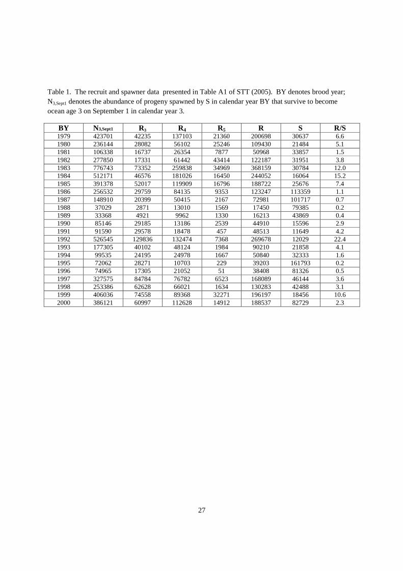
27

Table 1. The recruit and spawner data presented in Table A1 of STT (2005). BY denotes brood year; N3,Sept1 denotes the abundance of progeny spawned by S in calendar year BY that survive to become ocean age 3 on September 1 in calendar year 3.

BY N3,Sept1 R3 R4 R5 R S R/S 1979 423701 42235 137103 21360 200698 30637 6.6 1980 236144 28082 56102 25246 109430 21484 5.1 1981 106338 16737 26354 7877 50968 33857 1.5 1982 277850 17331 61442 43414 122187 31951 3.8 1983 776743 73352 259838 34969 368159 30784 12.0 1984 512171 46576 181026 16450 244052 16064 15.2 1985 391378 52017 119909 16796 188722 25676 7.4 1986 256532 29759 84135 9353 123247 113359 1.1 1987 148910 20399 50415 2167 72981 101717 0.7 1988 37029 2871 13010 1569 17450 79385 0.2 1989 33368 4921 9962 1330 16213 43869 0.4 1990 85146 29185 13186 2539 44910 15596 2.9 1991 91590 29578 18478 457 48513 11649 4.2 1992 526545 129836 132474 7368 269678 12029 22.4 1993 177305 40102 48124 1984 90210 21858 4.1 1994 99535 24195 24978 1667 50840 32333 1.6 1995 72062 28271 10703 229 39203 161793 0.2 1996 74965 17305 21052 51 38408 81326 0.5 1997 327575 84784 76782 6523 168089 46144 3.6 1998 253386 62628 66021 1634 130283 42488 3.1 1999 406036 74558 89368 32271 196197 18456 10.6 2000 386121 60997 112628 14912 188537 82729 2.3

28

Table 2. Iron Gate Hatchery (IGH) and Trinity River Hatchery (TRH) fingerling early survival (May – August) after release, spawner abundance from the Klamath River (KR), Trinity River (TR), and Unknown (UN), and the weights for Klamath River (wKR) and Trinity River (wTR) and final survival index s’ used in the STT (2005) analysis.

BY s′IGH s′TRH SKR STR SUN wKR wTR s′ 1979 0.0522 0.0589 21141 8028 1468 0.725 0.275 0.0540 1980 0.0183 0.0071 12383 7700 1400 0.617 0.383 0.0140 1981 0.0329 0.0058 17517 15340 1000 0.533 0.467 0.0202 1982 0.0058 0.0133 21177 9274 1500 0.695 0.305 0.0081 1983 0.0279 0.0870 12230 17284 1270 0.414 0.586 0.0625 1984 0.0255 0.0656 9420 5654 990 0.625 0.375 0.0405 1985 0.0174 0.0814 12166 9217 4294 0.569 0.431 0.0450 1986 0.0011 0.0050 15893 92548 4919 0.147 0.853 0.0044 1987 0.0015 0.0047 26511 71920 3286 0.269 0.731 0.0038 1988 0.0010 0.0034 29783 44616 4987 0.400 0.600 0.0024 1989 0.0005 0.0004 10584 29445 3839 0.264 0.736 0.0004 1990 0.0235 *0.0356 7102 7682 812 0.480 0.520 0.0298 1991 0.0045 0.0164 5905 4867 877 0.548 0.452 0.0099 1992 0.0447 0.0575 4135 7139 754 0.367 0.633 0.0528 1993 0.0018 0.0035 13385 5905 2568 0.694 0.306 0.0023 1994 0.0029 0.0070 20003 10906 1424 0.647 0.353 0.0043 1995 0.0028 0.0053 79851 77876 4067 0.506 0.494 0.0040 1996 0.0053 0.0106 31755 42646 6925 0.427 0.573 0.0083 1997 0.0668 0.0419 29015 11507 5622 0.716 0.284 0.0597 1998 0.0194 0.0083 16407 24460 1621 0.401 0.599 0.0128 1999 0.0263 0.0265 10883 6797 777 0.616 0.384 0.0264 2000 0.0123 0.0421 58388 24340 0 0.706 0.294 0.0211

* imputed value: ŝ′TRH,1990 = exp(0.89sIGH,1990).

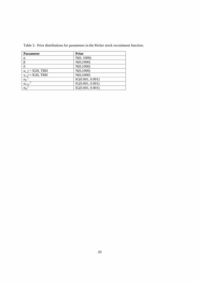
29

Table 3. Prior distributions for parameters in the Ricker stock recruitment function.

Parameter Prior α N(0, 1000) β N(0,1000) δ N(0,1000) κj, j = IGH, TRH N(0,1000) γj, j = IGH, TRH N(0,1000) σE

2 IG(0.001, 0.001) σCVI

2 IG(0.001, 0.001) σH

2 IG(0.001, 0.001)

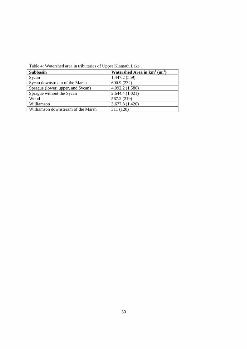
30

Table 4: Watershed area in tributaries of Upper Klamath Lake .

Subbasin Watershed Area in km2 (mi2) Sycan 1,447.2 (559) Sycan downstream of the Marsh 600.9 (232) Sprague (lower, upper, and Sycan) 4,092.2 (1,580) Sprague without the Sycan 2,644.4 (1,021) Wood 567.2 (219) Williamson 3,677.8 (1,420) Williamson downstream of the Marsh 311 (120)

31

Table 5. Posterior distribution mean, median and end points for 95% credible interval (2.5% and 97.5%) for parameters in the Ricker stock recruitment function.

Parameter Mean 2.5% 50% 97.5% α 2.48 1.90 2.48 3.05 β 1.73e-05 2.54e-05 1.71e-05 9.16e-06 δ 6.12e-01 3.24e-01 6.03e-01 9.27e-01 κIGH -4.77 -5.41 -4.76 -4.15 κTRH -4.30 -4.89 -4.30 -3.74 γIGH 6.44e-01 3.35e-01 6.41e-01 9.41e-01 γTRH 3.06e-01 -3.80e-02 3.12e-01 6.13e-01 σE 6.08e-01 3.65e-01 6.02e-01 8.85e-01 σCVI 1.27 8.78e-01 1.25 1.80 σH 5.07e-01 3.68e-01 4.93e-01 7.44e-01

32

Table 6. Probability distributions of the fishery reference points: spawner abundance that provides maximum sustainable yield (Smsy); spawner abundance that provides maximum recruitment (Smax); and the spawner abundance that is equal to recruitment at age 3 in the ocean (Sueq).

Reference Point Median 2.5% 97.5% Smsy 48,475 34,924.9 86,141.3 Smax 58,360.9 39,325.6 109,167.1 Sueq 143,660.4 106,406.9 232,915.5

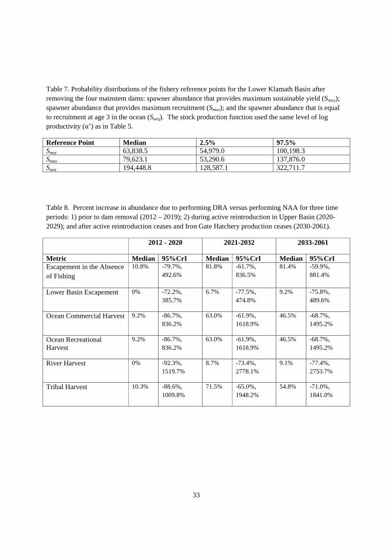
33

Table 7. Probability distributions of the fishery reference points for the Lower Klamath Basin after removing the four mainstem dams: spawner abundance that provides maximum sustainable yield (Smsy); spawner abundance that provides maximum recruitment (Smax); and the spawner abundance that is equal to recruitment at age 3 in the ocean (Sueq). The stock production function used the same level of log productivity (α’) as in Table 5.

Reference Point Median 2.5% 97.5% Smsy 63,838.5 54,979.0 100,198.3 Smax 79,623.1 53,290.6 137,876.0 Sueq 194,448.8 128,587.1 322,711.7

Table 8. Percent increase in abundance due to performing DRA versus performing NAA for three time periods: 1) prior to dam removal (2012 – 2019); 2) during active reintroduction in Upper Basin (2020-2029); and after active reintroduction ceases and Iron Gate Hatchery production ceases (2030-2061).

2012 - 2020 2021-2032 2033-2061

Metric Median 95%CrI Median 95%CrI Median 95%CrI Escapement in the Absence of Fishing

10.8% -79.7%, 492.6%

81.8% -61.7%, 836.5%

81.4% -59.9%, 881.4%

Lower Basin Escapement 0% -72.2%, 385.7%

6.7% -77.5%, 474.8%

9.2% -75.8%, 489.6%

Ocean Commercial Harvest 9.2% -86.7%, 836.2%

63.0% -61.9%, 1618.9%

46.5% -68.7%, 1495.2%

Ocean Recreational Harvest

9.2% -86.7%, 836.2%

63.0% -61.9%, 1618.9%

46.5% -68.7%, 1495.2%

River Harvest 0% -92.3%, 1519.7%

8.7% -73.4%, 2778.1%

9.1% -77.4%, 2753.7%

Tribal Harvest 10.3% -88.6%, 1009.8%

71.5% -65.0%, 1948.2%

54.8% -71.0%, 1841.0%

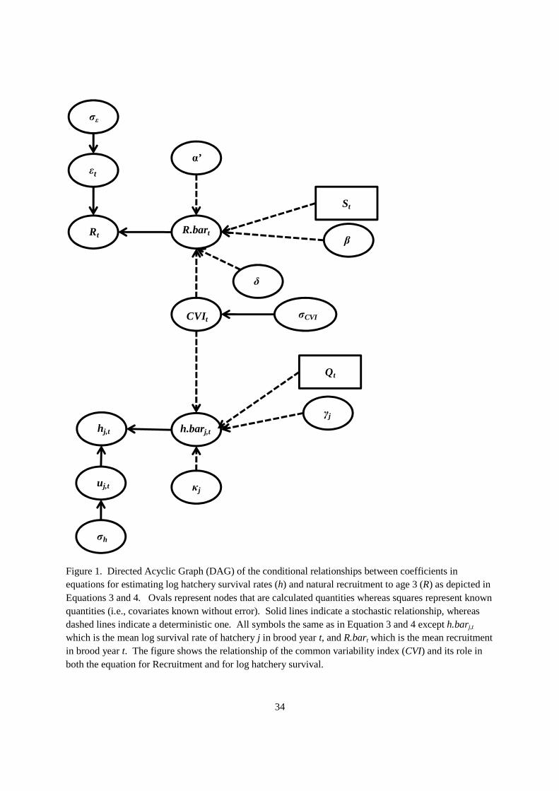
34

Figure 1. Directed Acyclic Graph (DAG) of the conditional relationships between coefficients in equations for estimating log hatchery survival rates (h) and natural recruitment to age 3 (R) as depicted in Equations 3 and 4. Ovals represent nodes that are calculated quantities whereas squares represent known quantities (i.e., covariates known without error). Solid lines indicate a stochastic relationship, whereas dashed lines indicate a deterministic one. All symbols the same as in Equation 3 and 4 except h.barj,t which is the mean log survival rate of hatchery j in brood year t, and R.bart which is the mean recruitment in brood year t. The figure shows the relationship of the common variability index (CVI) and its role in both the equation for Recruitment and for log hatchery survival.

α’

CVIt

hj,t

uj,t

h.barj,t

κj

γj

Qt

Rt

εt

R.bart

δ

β

St

σCVI

σε

σh

35

Figure 2. Flow forecasts for 2012 to 2061 under NMFS Biological Opinion (BO) and under KBRA in the Klamath River at Seiad during July. Flow values were standardized using the mean Klamath River flows in July at Seiad Valley from 1980 to 2000 (mean = 1589, sd = 944.17). The standardized flow values were incorporated in the model for forecasts of abundance and harvest under NAA and DRA.

2020 2030 2040 2050 2060

-10

12

3

Year

Sta

ndar

dize

d flo

w

KBRABO

36

Figure 3. Depiction of sampling from higher percentiles of a hypothetical productivity distribution over time. Samples of productivity occur only from the Accepted region. Early in the time series, samples from almost the entire distribution are accepted (Top, Accepted threshold at 0.05 quantile). Later in the time series, the Accepted region is shifted to the right due to higher expected productivity (Middle, Accepted threshold at the 0.10 quantile). At the end of the time series the threshold for the Accepted region has again shifted towards higher productivity (Bottom, Accepted threshold at the 0.25 quantile).

0 1 2 3 4 5

0.0

0.2

0.4

0.6

0.8

1.0

Den

sity

Rejected Accepted

0 1 2 3 4 5

0.0

0.2

0.4

0.6

0.8

1.0

Den

sity

Rejected Accepted

0 1 2 3 4 5

0.0

0.2

0.4

0.6

0.8

1.0

Den

sity

Rejected Accepted

37

Figure 4. Median predicted ocean age 3 recruits from the Ricker stock recruitment model and observed ocean age 3.

0e+00 2e+05 4e+05 6e+05 8e+05

0e+0

02e

+05

4e+0

56e

+05

8e+0

5

Observed Age 3 Ocean

Pre

dict

ed A

ge 3

Oce

an

38

Figure 5. Observed log survival rates from Iron Gate Hatchery (A) and Trinity River Hatchery (B) with median model predictions and 95% credible intervals (95% CrI).

1980 1985 1990 1995 2000

-8-6

-4-2

Iron Gate Hatchery

Year

log

surv

ival

A

1980 1985 1990 1995 2000

-8-6

-4-2

Trinity River Hatchery

Year

log

surv

ival

B

Median95% CrI

39

Figure 6. The common variability index (CVI) from 1979 to 2000, which is the annual variability common to both Iron Gate Hatchery and Trinity River Hatchery fingering CWT release groups estimated from log hatchery survival rates.

1980 1985 1990 1995 2000

-3-2

-10

12

3

Year

CV

I

median95% CrI

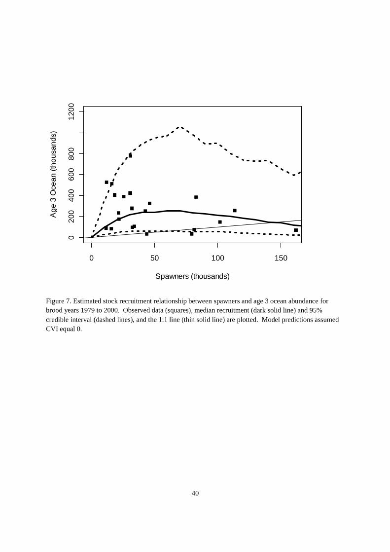
40

Figure 7. Estimated stock recruitment relationship between spawners and age 3 ocean abundance for brood years 1979 to 2000. Observed data (squares), median recruitment (dark solid line) and 95% credible interval (dashed lines), and the 1:1 line (thin solid line) are plotted. Model predictions assumed CVI equal 0.

0 50 100 150

020

040

060

080

012

00

Spawners (thousands)

Age

3 O

cean

(tho

usan

ds)

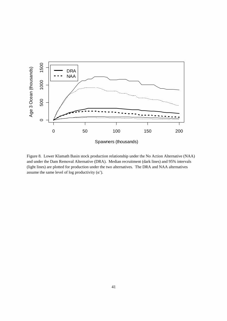
41

Figure 8. Lower Klamath Basin stock production relationship under the No Action Alternative (NAA) and under the Dam Removal Alternative (DRA). Median recruitment (dark lines) and 95% intervals (light lines) are plotted for production under the two alternatives. The DRA and NAA alternatives assume the same level of log productivity (α’).

0 50 100 150 200

050

010

0015

00

Spawners (thousands)

Age

3 O

cean

(tho

usan

ds)

DRANAA

42

Figure 9. Distribution of .log productivity (α’) in the lower Klamath Basin from 2012 to 2061 due to habitat restoration by KBRA.

2020 2030 2040 2050 2060

1.5

2.0

2.5

3.0

3.5

Year

log

prod

uctiv

ity

median95%CrI

43

Figure 10. Stock recruitment relationship in the lower Klamath basin in 2025 and in 2055 including increase in habitat due to dam removal and KBRA actions affecting log productivity α’ *. Median production (dark line) and 95%I (light line) are plotted for each of the two years.

0 50 100 150 200

050

010

0015

00

Spawners (thousands)

Age

3 O

cean

(tho

usan

ds)

20252055

44

Figure 11. Distribution of log productivity (rnew*) of a mixed stream and ocean type life history in

tributaries to Upper Klamath Basin from 2012 to 206. Changes in log productivity over the time series are due to habitat restoration by KBRA.

2020 2030 2040 2050 2060

1.0

1.5

2.0

2.5

3.0

Year

log

prod

uctiv

ity

median95%CrI

45

Figure 12. Stock recruitment relationship in the tributaries to Upper Klamath Lake in 2020 and in 2055 incorporating mixed stream and ocean type life history and KBRA actions affecting log productivity

rnew*. Median production (dark line) and 95%I (light line) are plotted for each of the two years.

0 20 40 60 80

050

100

200

300

Spawners (thousands)

Age

3 O

cean

(tho

usan

ds) 2025

2055

46

Figure 13. Probability that escapement in the absence of fishing is greater under DRA than under NAA from 2012 to 2061 (top). Dashed line represents 50/50 chance of increased abundance under DRA. Median and 95% credible intervals for the percent increase in DRA relative to NAA from 2012 to 2061 (bottom). Dashed line represents no difference between DRA and NAA.

2020 2030 2040 2050 2060

0.0

0.2

0.4

0.6

0.8

1.0

Escapement in Absence of Fishing

Pro

porti

on D

RA

> N

AA

Harvest Rule: Modified Council Rule 2011

2020 2030 2040 2050 2060

0

500

1000

Year

Per

cent

Diff

eren

ce (D

RA

- N

AA

)

Median95%CrI

47

Figure 14. Probability that escapement to the Lower Klamath Basin is greater under DRA than under NAA from 2012 to 2061 (top). Dashed line represents 50/50 chance of increased abundance under DRA. Median and 95% credible intervals for the percent increase in DRA relative to NAA from 2012 to 2061 (bottom). Dashed line represents no difference between DRA and NAA.

2020 2030 2040 2050 2060

0.0

0.2

0.4

0.6

0.8

1.0

Escapement to Lower Basin

Pro

porti

on D

RA

> N

AA

Harvest Rule: Modified Council Rule 2011

2020 2030 2040 2050 2060

-200

0

200

400

600

800

Year

Per

cent

Diff

eren

ce (D

RA

- N

AA

)

Median95%CrI

48

Figure 15. Probability that ocean commercial harvest is greater under DRA than under NAA from 2012 to 2061 (top). Dashed line represents 50/50 chance of increased abundance under DRA. Median and 95% credible intervals for the percent increase in DRA relative to NAA from 2012 to 2061 (bottom). Dashed line represents no difference between DRA and NAA.

2020 2030 2040 2050 2060

0.0

0.2

0.4

0.6

0.8

1.0

Ocean Commercial Harvest

Pro

porti

on D

RA

> N

AA

Harvest Rule: Modified Council Rule 2011

2020 2030 2040 2050 2060

0

500

1000

1500

2000

Year

Per

cent

Diff

eren

ce (D

RA

- N

AA

)

Median95%CrI

49

Figure 16. Probability that ocean recreational harvest is greater under DRA than under NAA from 2012 to 2061 (top). Dashed line represents 50/50 chance of increased abundance under DRA. Median and 95% credible intervals for the percent increase in DRA relative to NAA from 2012 to 2061 (bottom). Dashed line represents no difference between DRA and NAA.

2020 2030 2040 2050 2060

0.0

0.2

0.4

0.6

0.8

1.0

Ocean Recreational Harvest

Pro

porti

on D

RA

> N

AA

Harvest Rule: Modified Council Rule 2011

2020 2030 2040 2050 2060

0

500

1000

1500

2000

Year

Per

cent

Diff

eren

ce (D

RA

- N

AA

)

Median95%CrI

50

Figure 17. Probability that river harvest is greater under DRA than under NAA from 2012 to 2061 (top). Dashed line represents 50/50 chance of increased abundance under DRA. Median and 95% credible intervals for the percent increase in DRA relative to NAA from 2012 to 2061 (bottom). Dashed line represents no difference between DRA and NAA.

2020 2030 2040 2050 2060

0.0

0.2

0.4

0.6

0.8

1.0

River Harvest

Pro

porti

on D

RA

> N

AA

Harvest Rule: Modified Council Rule 2011

2020 2030 2040 2050 2060

0

1000

2000

3000

4000

Year

Per

cent

Diff

eren

ce (D

RA

- N

AA

)

Median95%CrI

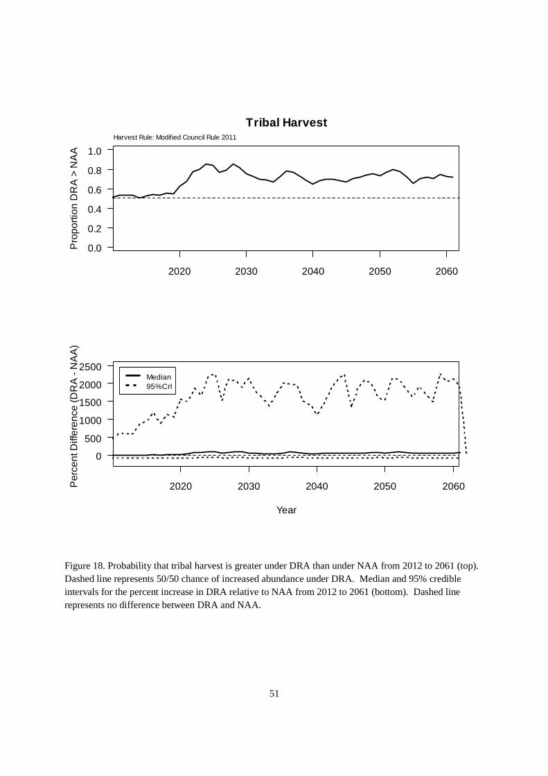
51

Figure 18. Probability that tribal harvest is greater under DRA than under NAA from 2012 to 2061 (top). Dashed line represents 50/50 chance of increased abundance under DRA. Median and 95% credible intervals for the percent increase in DRA relative to NAA from 2012 to 2061 (bottom). Dashed line represents no difference between DRA and NAA.

2020 2030 2040 2050 2060

0.0

0.2

0.4

0.6

0.8

1.0

Tribal Harvest

Pro

porti

on D

RA

> N

AA

Harvest Rule: Modified Council Rule 2011

2020 2030 2040 2050 2060

0

500

1000

1500

2000

2500

Year

Per

cent

Diff

eren

ce (D

RA

- N

AA

)

Median95%CrI

52

Appendix A. Fishery Control Rule Applied in the Klamath Harvest Rate Model

Figure A2.1. Harvest rate as a function of escapement in the absence of fishing utilized in the Klamath Harvest Rate Model (Mohr et al. in Prep).

Management of the Klamath Fishery was modeled by the Klamath Harvest Rate Model (KHRM, Mohr et al. in Prep.). Integral to the KHRM is the definition of a fishery control rule that defines the harvest rate as a function of an unfished escapement estimate (Figure 1). The fishery control rule described here provides the opportunity for a de minimis fishery even if the escapement in the absence of fishing is below the target stock size of 40,700 (Smsy).

0 50000 100000 150000

0.0

0.1

0.2

0.3

0.4

0.5

0.6

0.7

Escapement in the Absence of Fishing

Har

vest

Rat

e

53

Appendix B. Pseudocode for running the No Action Alternative and the Dam Removal Alternative

A. Steps to Running NAA

Set initial abundances and parameter values

The following steps were completed prior to running the annual forecasts of recruitment and harvest by drawing 1000 values from the following distributions (note that N(mean, variance) refers to a normal distribution with mean and variance as specified):

1. Set initial abundances from the CDFG MegaTable (CDFG 2011) a. Spawning abundance in 2007 distributed as N(61741, 25000) b. Spawning abundance in 2008 distributed as N(48073, 25000) c. Spawning abundance in 2009 distributed as N(52499, 25000) d. Spawning abundance in 2010 distributed as N(49027, 25000)

2. Set initial abundances in the ocean in 2010 (PFMC 2011 PreSeason Report) a. Age 4 in the ocean in 2010 distributed as N(66500, 25000) b. Age 5 in the ocean in 2010 distributed as N(700, 250)

3. Set initial proportion of natural fish in the ocean in 2010 a. Proportion of natural age 4 in 2010, g4 = 0.5 b. Proportion of natural age 5in 2010, g5 = 0.5

4. Draw parameter values from samples of the posterior distribution from the Ricker stock-recruitment model for natural production (Table 4)

a. Productivity, α’ b. Ricker density dependence parameter, β c. Strength of CVI on natural stocks, δ d. Standard deviation of random effect CVI, σCVI

2 e. The values of CVI for each year of the time series, CVI2007:2061~N(0, σCVI

2) 5. Draw parameter values from samples of the posterior distribution from the Ricker stock-

recruitment model for hatchery log survival (Table 4). Hatchery production was constant over the 2007 to 2061 time series with IGH production of 6 million, and TRH production of 3 million fingerlings.

a. Average log hatchery survival, κIGH and κTRH b. Parameter relating log survival to flow, γIGH and γTRH

c. Standard deviation for residual variability on log hatchery survival, N2 d. Unexplained variability of log hatchery survival u1:2, 2010:2061

With the initial abundance estimates specified, and the vectors of parameter values specified, the dynamic portion of the model could be completed.

Calculate annual production and harvest

For iteration i = 1 to 1000 (subscript suppressed for clairity)

For years t = 2010 to 2061

54

1. Calculate natural production of the age 3 ocean fish in year t by.

�� = ��−3exp { �′ − ���−3 + � ���−2 + �� } Equation 2A13 2. Calculate the survival rate of IGH releases for year t, sIGH, using Klamath River Biological

Opinion flows .

_�`N,� . exp {ℎ�`N,�} = exp {��`N + ���−2 + ��`N (�a�_cd,�−2) + ��`N,�} Equation (A2)

3. Calculate the survival rate of TRH releases for brood year t, sTRH, using Trinity River flows

_efg,� . exp {ℎefg,�} . exp {�efg + ��� h + �efg ��ef,� h� + �efg,�} Equation (A3)

4. Calculate the hatchery production to age 3 assuming age 2 survival of 0.5 (Hankin and Logan 2010) for year t

g,� . 0.52 _�lg,� 6�06 + _efg,� 3�063 Equation (A4)

5. Calculate the total abundance of year 3 ocean fish

n,� . �� + g,� Equation (A5)

6. Calculate the proportion of year 3 ocean fish that are natural origin

1n,� . fofop qr,o

Equation (A6)

7. Call KHRM and pass Na,t ={N3,t , N4,t , N5,t }and ga,t ={g3,t , g4,t , g5,t } 8. In year t KHRM returns:

a. Natural area escapement, En which is set equal to St b. Harvest

i. Ocean commercial harvest, Hu ii. Ocean recreational harvest, Hw iii. River tribal harvest, Ht iv. River recreational harvest, Hr

c. Ocean Abundance in year t + 1 i. 4 year old abundance in the ocean N’4

ii. 5 year old abundance in the ocean, N’5

Next year: Repeat the loop for year t+1 by returning to step 1 having obtained the ocean abundances for the 4 and 5 year olds returned from KHRM

Next iteration

2.2.3 Steps to Running DRA

Set initial abundances and parameter values

55

The following steps were completed prior to running the annual forecasts of recruitment and harvest for iterations i = 1 to 1000, the subscript for iteration i is suppressed for clarity.

1. Use initial abundances previously sampled for the NAA alternative a. Spawning abundance in 2007 b. Spawning abundance in 2008 c. Spawning abundance in 2009 d. Spawning abundance in 2010

2. Use initial abundances in the ocean in 2010 previously sampled for the NAA a. Age 4 in the ocean in 2010 b. Age 5 in the ocean in 2010

3. Use initial proportion of natural fish in the ocean in 2010 from NAA a. Proportion of natural age 4 in 2010, g4 = 0.5 b. Proportion of natural age 5in 2010, g5 = 0.5

4. Lower Basin stock recruitment parameters for years 2010 to 2020 a. Productivity drawn from truncated α’ starting in 2012 to reduce the probability of low

productivity as a result of KBRA b. Ricker density dependence parameter, β c. Strength of CVI on natural stocks, use draws of δ from the NAA d. Use the values of CVI from the NAA, CVI2010:2020

5. Lower Basin stock recruitment parameters for 2021 to 2061 a. Productivity drawn from truncated α’ starting in 2012 to reduce the probability of low

productivity as a result of KBRA b. Ricker density dependence parameter based on additional spawning habitat from Iron

Gate to Keno and tributaries, βnew c. Strength of CVI on natural stocks, use draws of δ from the NAA d. Use the values of CVI from the NAA, CVI2021:2061

6. Hatchery production from 2010 to 2028. Hatchery production was constant over the 2010 to 2020 with IGH production of 6 million, and TRH production of 3 million fingerlings.

a. Use draws of average log hatchery survival, κIGH and κTRH from NAA b. Use draws of parameter relating log survival to flow, γIGH and γTRH from NAA c. Use draws of unexplained variability of log hatchery survival u1:2, 2010:2028 from NAA

7. Hatchery production from 2029 to 2061. Hatchery production was assumed constant at TRH with production of 3 million fingerlings, whereas production at IGH ceases after 2028.

a. Use draws of average log hatchery survival, κTRH from NAA b. Use draws of parameter relating log survival to flow, γTRH from NAA c. Use draws of unexplained variability of log hatchery survival at TRH u2, 2029:2061 from

NAA 8. Stock recruitment parameters in tributaries to UKL in years t = 2021, …, 2061

a. Unfished equilibrium population size, Enew, t i. Draw a value of p,t from a Uniform(0,1) distribution in year t

ii. Sample from the distribution of Enew stream using the watershed size of 4200.96 km2

56

iii. Sample from the distribution of Enew ocean using the watershed size of 4200.96 km2

iv. Calculate , Enew, t using Equation 17 b. Productivity, rnew, t

i. Sample from the truncated distribution of rnewocean with the degree of truncation dependent upon the year

ii. Sample from the truncated distribution of rnewstream with the degree of truncation dependent upon the year

iii. Calculate rnew,t, using Equation 18.

With the initial abundance estimates specified, and the vectors of parameter values specified, the dynamic portion of the model could be completed.

Calculate annual production and harvest

For iteration i = 1 to 1000 (subscript suppressed for clairity)

For years t = 2010 to 2020

1. Calculate natural production of the age 3 ocean fish in year t, Rt in the lower basin using Equation 10; however replace α’ with the samples from the truncated α’ *

(the asterisk denotes draws from a truncated distribution).

2. Calculate the survival rate of IGH releases for year t, sIGH,t using Equation 11 and calculate the survival rate of TRH releases for year t, sTRHt using Equation 12. Note that the survival rates are the same as used in the NAA due to using the draws from the posterior distributions for parameters used in Equations 11 and 12.

3. Calculate the hatchery production to age 3 assuming age 2 survival of 0.5 (Hankin and Logan 2010) for year t using Equation 13.

4. Calculate the total abundance of year 3 ocean fish using Equation 14. 5. Calculate the proportion of year 3 ocean fish that are natural origin using Equation 15. 6. Call KHRM and pass Na,t ={N3,t , N4,t , N5,t }and ga,t ={g3,t , g4,t , g5,t } 7. The KHRM program returns:

a. Natural area escapement, En which is set equal to St b. Harvest

i. Ocean commercial harvest, Hu ii. Ocean recreational harvest, Hw iii. River tribal harvest, Ht iv. River recreational harvest, Hr

c. Ocean Abundance in year t + 1 i. 4 year old abundance in the ocean N’4

ii. 5 year old abundance in the ocean, N’5

Next year: Repeat the loop for year t+1 by returning to step 1 having obtained the ocean abundances for the 4 and 5 year olds returned from KHRM

57

For years t > 2020

1. Calculate natural production of the age 3 ocean fish in year t, Rt in the lower basin using Equation 10; however replace α’ with the samples from the truncated α’ *

(the asterisk denotes draws from a truncated distribution) and the new capacity βnew.

�� . �� nexp { � ′∗ − �6,7�� n + � ��� h + �� } Equation 2A73 2. If t < 2032 the reintroduction program in the tributaries to UKL provides spawners (SUKL,t) at

levels equal to or greater than capacity SUKL,t = max(Enew,t, S UKL,t) 3. For t > 2022, calculate recruitment of age 3 ocean fish from production in the tributaries to UKL

(RUKL,t) incorporating the truncated mixture of ocean and stream type Chinook, the common variability among basins (CVI), and flow related survival. Finally, recruitment to the adult stage is multiplied by an adult return to age 3 in the ocean conversion factor (CF) obtained from Table 1.

�tuv,� . �tuv,� n exp wC. x�y∗ z1 − "o{|}IGJ,o

~ + � ��� h + ��lg�u�f�,� h � � Equation (A8)

4. If year t > 2028 IGH ceases to produce fall Chinook and hatchery production consists of TRH fish only of 3 million

�,� . 0.52 _efg,� 3�063 Equation (A9)

5. Calculate total natural production of natural origin age 3 fish

6,� . �� + �tuv,�

6. Calculate the proportion of lower basin natural production relative to the total natural production for age 3 fish in year t . Note that values of l4,t = l3,t-1 and likewise l5,t = l4,t-1 so that the proportion of lower basin natural production could track the different cohorts moving through the fishery

/n,� . fofop f���,o Equation (A10)

7. Calculate total production of age 3 fish on September 1

n,� . 6,� + �,� Equation (A11)

8. Calculate the proportion of year 3 ocean fish that are natural origin

1n,� . qI,oqI,op q�,o

Equation (A12)

9. Call KHRM and pass Na,t ={N3,t , N4,t , N5,t }and ga,t ={g3,t , g4,t , g5,t } 10. In year t KHRM returns:

a. Age specific natural area escapement, Ena which is split between lower basin and UKL tributary production using the appropriate age-specific values of la,t . .

�� . ∑ 56,) /),��)�n Equation (A13)

58

�tuv,� . ∑ 56,) 21 − /),�3�)�n Equation (A14)

b. Harvest i. Ocean commercial harvest, Hu

ii. Ocean recreational harvest, Hw iii. River tribal harvest, Ht iv. River recreational harvest, Hr

c. Ocean Abundance in year t + 1 i. 4 year old abundance in the ocean N’4

ii. 5 year old abundance in the ocean, N’5

Next year: Repeat the loop for year t+1 by returning to step 1 having obtained the ocean abundances for the 4 and 5 year olds returned from KHRM

Next iteration