NREL is a national laboratory of the U.S. Department of Energy Office of Energy Efficiency & Renewable Energy Operated by the Alliance for Sustainable Energy, LLC

This report is available at no cost from the National Renewable Energy Laboratory (NREL) at www.nrel.gov/publications.

Contract No. DE-AC36-08GO28308

Summary of Market Opportunities for Electric Vehicles and Dispatchable Load in Electrolyzers Report of Work in Completion of Deliverable: “Report on Identified Values of EVGI Strategies”

Paul Denholm, Joshua Eichman, and Tony Markel National Renewable Energy Laboratory

Ookie Ma U.S. Department of Energy

Technical Report NREL/TP-6A20-64172 May 2015

NREL is a national laboratory of the U.S. Department of Energy Office of Energy Efficiency & Renewable Energy Operated by the Alliance for Sustainable Energy, LLC

This report is available at no cost from the National Renewable Energy Laboratory (NREL) at www.nrel.gov/publications.

Contract No. DE-AC36-08GO28308

National Renewable Energy Laboratory 15013 Denver West Parkway Golden, CO 80401 303-275-3000 • www.nrel.gov

Summary of Market Opportunities for Electric Vehicles and Dispatchable Load in Electrolyzers Report of Work in Completion of Deliverable: “Report on Identified Values of EVGI Strategies” Paul Denholm, Joshua Eichman, and Tony Markel National Renewable Energy Laboratory

Ookie Ma U.S. Department of Energy

Prepared under Task Nos. VTP2IN13 and HT12IN30

Technical Report NREL/TP-6A20-64172 May 2015

NOTICE

This report was prepared as an account of work sponsored by an agency of the United States government. Neither the United States government nor any agency thereof, nor any of their employees, makes any warranty, express or implied, or assumes any legal liability or responsibility for the accuracy, completeness, or usefulness of any information, apparatus, product, or process disclosed, or represents that its use would not infringe privately owned rights. Reference herein to any specific commercial product, process, or service by trade name, trademark, manufacturer, or otherwise does not necessarily constitute or imply its endorsement, recommendation, or favoring by the United States government or any agency thereof. The views and opinions of authors expressed herein do not necessarily state or reflect those of the United States government or any agency thereof.

This report is available at no cost from the National Renewable Energy Laboratory (NREL) at www.nrel.gov/publications.

Available electronically at SciTech Connect http:/www.osti.gov/scitech

Available for a processing fee to U.S. Department of Energy and its contractors, in paper, from:

U.S. Department of Energy Office of Scientific and Technical Information P.O. Box 62 Oak Ridge, TN 37831-0062 OSTI http://www.osti.gov Phone: 865.576.8401 Fax: 865.576.5728 Email: reports@osti.gov

Available for sale to the public, in paper, from:

U.S. Department of Commerce National Technical Information Service 5301 Shawnee Road Alexandra, VA 22312 NTIS http://www.ntis.gov Phone: 800.553.6847 or 703.605.6000 Fax: 703.605.6900 Email: orders@ntis.gov

Cover Photos by Dennis Schroeder: (left to right) NREL 26173, NREL 18302, NREL 19758, NREL 29642, NREL 19795.

NREL prints on paper that contains recycled content.

Acknowledgments This project was funded by the U.S. Department of Energy Vehicles Technologies Office and Fuel Cell Technologies Office. The following individuals provided valuable input during the publication process: Aaron Bloom, Jaquelin Cochran, Kevin Harrison, and Mike Meshek. Any errors or omissions are the sole responsibility of the authors.

iii

Executive Summary Electric vehicles (EVs) and electrolyzers are potentially significant sources of new electric loads. Both are flexible in that the amount of electricity consumed can be varied in response to a variety of factors including the cost of electricity. Because both EVs and electrolyzers can control the timing of electricity purchases, they can minimize energy costs by timing the purchases of energy to periods of lowest costs.

For EV charging, the goal should be to eliminate most or all capacity related charges in retail rate structures. In theory, a properly controlled EV should place no additional demand on either the generation or the distribution system and still allow full utilization for electric travel. Therefore, it should be able to charge with energy for only the variable costs of generation. Existing rate structures and demand programs allow for some reduction in capacity costs; however, programs that come closest to allowing the highest level of scheduling control such as demand-based rates or real-time pricing are relatively rare for residential consumers. The provision of ancillary services from EV charging has the potential to provide some additional value; however, the overall revenue opportunities are small relative to the benefits of reduced costs associated with controlled charging.

For electrolyzer use, timing of production can also act to reduce both capacity and energy costs. The primary tradeoff will be between equipment utilization and cost minimization. Sale of hydrogen is the main revenue stream and participation in electricity markets, new rate-structures, or DR programs provides a decrease in costs, but also potentially a decrease in production. As such, the value of participation that impacts the operation of electrolyzers must be weighed against the opportunity cost of produced hydrogen.

iv

Table of Contents 1 Introduction ........................................................................................................................................... 1 2 Electricity Services ............................................................................................................................... 2 3 Traditional Tariff Mechanisms via Load-Serving Entities ................................................................ 4

Standard Rate Structures ........................................................................................................................ 5 Traditional LSE Demand Response and Interruptible Load Programs ................................................ 14

Direct Load Control .................................................................................................................... 16 Interruptible Rates ....................................................................................................................... 17

Limitations of Rate Structures for Optimized EV Charging and Electrolyzer Use .............................. 20 4 Wholesale Market-Based Energy Transactions .............................................................................. 21 5 Ancillary Services ............................................................................................................................... 25

Technical Requirements ....................................................................................................................... 26 Cost ..................................................................................................................................................... 27 Market Size ........................................................................................................................................... 32 Impact of Variable Generation on Market Size .................................................................................... 36

6 Conclusions ........................................................................................................................................ 38 7 References .......................................................................................................................................... 39

v

List of Figures Figure 1. Mechanisms for purchase of electricity either (a) through an LSE or (b) directly from

the market ................................................................................................................................. 3 Figure 2. Electricity sales via a load-serving entity ...................................................................................... 4 Figure 3. Locations with customer choice programs .................................................................................... 5 Figure 4. Tariff summary sheet for residential customers of Portland General Electric (PGE 2014) .......... 7 Figure 5. Example of identical energy use with different consumption patterns during a 24-hour period ... 8 Figure 6. Time-of-use periods in the Portland General Electric Residential Rate (PGE 2012) .................... 9 Figure 7. Demand patterns that demonstrate the limits of energy-only rates that do not capture variation in

capacity needs .......................................................................................................................... 9 Figure 8. Tariff summary sheet comparing energy-only and demand-based rates for residential PSCO

customers ............................................................................................................................... 10 Figure 9. Demand-based energy rates can offer low-cost energy for EV charging if appropriately timed.

The red line shows a demand profile for EV charging that would not raise peak demand, and hence the demand charges. ..................................................................................................... 11

Figure 10. Residential rate structures for Georgia Power ........................................................................... 13 Figure 11. Rate TOU-GSD-8 for Georgia Power ....................................................................................... 14 Figure 12. Hourly load profiles for the balancing area served by PSCO in 2003 ....................................... 15 Figure 13. Load duration curve for the balancing area served by PSCO, 2003 .......................................... 16 Figure 14. Tariff sheet summary for large customers of PSCO .................................................................. 18 Figure 15. Summary of the Interruptible Service Option Credit for large customers of PSCO ................. 19 Figure 16. Locations with restructured markets .......................................................................................... 21 Figure 17. Example of distribution-only tariffs for customers that take energy from a competitive energy

supplier ................................................................................................................................... 22 Figure 18. Seasonal price patterns for the PJM market in 2012 ................................................................. 24 Figure 19. Average and marginal wholesale price as a function of utilization ........................................... 25 Figure 20. Relative price of spinning reserves to regulating reserves in selected U.S. markets ................. 30 Figure 21. Average hourly prices for reserve services in NYISO and MISO in 2011 ................................ 30 Figure 22. Average hourly regulation up and down prices for ERCOT in 2012 ........................................ 31 Figure 23. Regulation requirements for PJM, June 8–9 2014 ..................................................................... 35

List of Tables Table 1. Selected Ancillary Service Tariffs in Non-ISO/RTO Balancing Authority Areas

(Ma et al. 2013) ..................................................................................................................... 28 Table 2. Selected Ancillary Service Prices in Several ISO/RTO Markets, 2002–2012a ............................ 29 Table 3. Regulation and Spinning Contingency Reserve Requirements in U.S. Wholesale Markets ........ 33 Table 4. Selected ancillary service tariffs and requirements in non-ISO/RTO balancing authority areas

(Ma et al. 2013) ...................................................................................................................... 34 Table 5. Estimated Increase in Regulation Required Due to the Addition of VG ...................................... 36

vi

1 Introduction Electric vehicles (EVs) and electrolyzers are potentially significant sources of new electric loads. Both are flexible in that the amount of electricity consumed can be varied in response to a variety of factors including the cost of electricity. Because both EVs and electrolyzers can control the timing of electricity purchases, they can minimize energy costs by timing the purchases of energy to periods of lowest costs. In addition, EV owners or electrolyzer operators may take advantage of demand response programs, which can further reduce electricity costs or provide revenue, again by timing demand and reducing load during periods when this reduction in demand represents a product that can be sold back to the grid.

This report summarizes the mechanisms by which EV or electrolyzer owners may minimize energy costs or derive revenue by providing grid services. It is important to note that we consider only the ability to control the demand for electricity from vehicle charging or electrolysis operation. Discharge of electricity (from an EV battery in vehicle to grid applications or use of stored hydrogen in fuel cells) is not considered. Section 2 provides an overview of electricity services and the two basic market mechanisms by which electricity services are purchased—via a load-serving entity (LSE) or via direct market transactions. Section 3 discusses electricity purchases via an LSE, and it provides an overview of basic rate structures, which are the primary driver of how residential, commercial, and many industrial customers can control costs. Section 3 also describes LSE-operated demand response programs, including interruptible rates and direct load control programs. Section 4 describes electricity purchases made via wholesale markets, including real-time pricing available from some LSEs. Section 5 provides an overview of ancillary services, including participation requirements, market size, and potential revenue opportunities.

1

2 Electricity Services Provision of reliable electricity requires capacity, energy, and ancillary services. Capacity represents the ability to generate and deliver energy, and it includes generation capacity as well as transmission and distribution system capacity. The cost of capacity is based primarily on fixed costs, which cover the carrying costs of the capital investments plus fixed operations and maintenance costs.

By contrast, the cost of energy is based largely on the variable costs of operating the power system, which are primarily fuel costs but also include variable operations and maintenance costs. Ancillary services are largely capacity services that help system operators maintain a reliable grid with sufficient power quality. These include operating reserves, representing capacity available to start up or increase output in response to random variation in demand, plant outages, or other contingencies.

Capacity, energy, and operating reserves have different units of measure. Electricity service, when referring to energy, is sold in units such as kilowatt-hours (kWh) or megawatt-hours (MWh). However, capacity and operating reserves involve the commitment of resources to offer energy during set times. This can, thereby, be measured in units of power (i.e., kW or MW) times the service duration. (Costs of capacity services are sometimes signified using a dash, such as kW-h, kW-month or kW-yr.) While provision of energy services involves the actual buying and selling of electricity, capacity and operating reserves provide the insurance that energy will be available when and where it is needed.

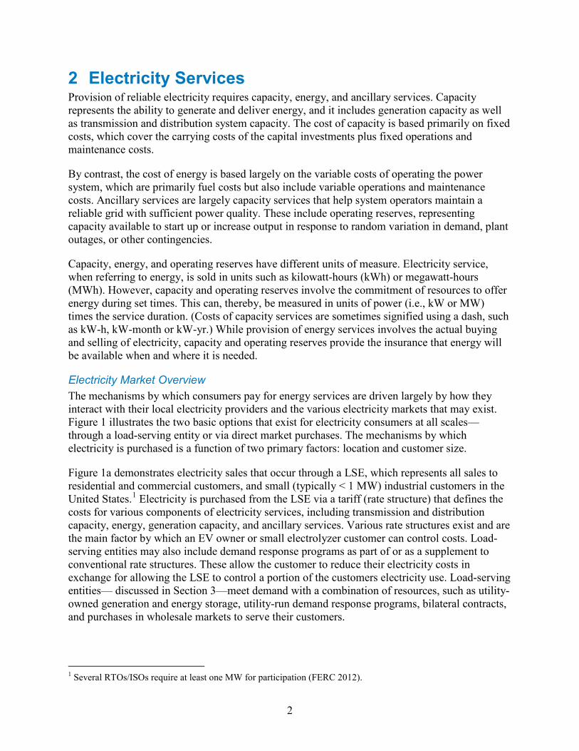
Electricity Market Overview The mechanisms by which consumers pay for energy services are driven largely by how they interact with their local electricity providers and the various electricity markets that may exist. Figure 1 illustrates the two basic options that exist for electricity consumers at all scales—through a load-serving entity or via direct market purchases. The mechanisms by which electricity is purchased is a function of two primary factors: location and customer size.

Figure 1a demonstrates electricity sales that occur through a LSE, which represents all sales to residential and commercial customers, and small (typically < 1 MW) industrial customers in the United States.1 Electricity is purchased from the LSE via a tariff (rate structure) that defines the costs for various components of electricity services, including transmission and distribution capacity, energy, generation capacity, and ancillary services. Various rate structures exist and are the main factor by which an EV owner or small electrolyzer customer can control costs. Load-serving entities may also include demand response programs as part of or as a supplement to conventional rate structures. These allow the customer to reduce their electricity costs in exchange for allowing the LSE to control a portion of the customers electricity use. Load-serving entities— discussed in Section 3—meet demand with a combination of resources, such as utility-owned generation and energy storage, utility-run demand response programs, bilateral contracts, and purchases in wholesale markets to serve their customers.

1 Several RTOs/ISOs require at least one MW for participation (FERC 2012).

2

Load serving entities and larger customers (typically 1>MW) transact with the wholesale market. The wholesale market includes independent power producers, other utilities, and in much of the United States, an independent system operator that coordinates electricity sales and operation. This larger marketplace operates via a variety of mechanisms, including bilateral contracts at various times scales, centralized markets, and other “behind-the-scenes” transactions, and the marketplace typically does not interact directly with residential or commercial electricity customers. However, there are new and emerging opportunities for retail customers to provide services to LSEs and the market, either directly or through an aggregator.

(a) LSE (b) Direct Market Purchases

DR = demand response

Figure 1. Mechanisms for purchase of electricity either (a) through an LSE or (b) directly from the market

The second mechanism for electricity sales (Figure 1b) allows very large electricity consumers to engage directly with the electricity marketplace, arranging for bulk electricity purchases through the various existing market mechanisms. They may use a local distribution network operator, or they may interconnect directly to the transmission network (effectively owning and operating their own distribution system). These consumers are typically large industries whose electricity demand warrants the cost and complexity of arranging their own purchases of electricity.

Market

Load ServingEntity

ConventionalTariff

Traditional LSE DRprogram

Market

Market-based DR program

Aggregator

3

3 Traditional Tariff Mechanisms via Load-Serving Entities

The majority of electricity consumed in the United States is delivered by an LSE (EIA 2013). Only industrial customers, typically with loads typically greater than 1 MW, can purchase electricity directly from a wholesale market, bypassing an LSE.2 The cost of electricity is set through a rate structure established by the LSE, which includes traditional vertically-integrated utilities or competitive electricity suppliers, illustrated in Figure 2. Figure 2a shows the process by which consumers purchase electricity from a vertically integrated utility. The utility depicted in the figure owns and operates the distribution, transmission, and much of the generation infrastructure used to deliver reliable electricity to the end consumer.

(a) Vertically Integrated Utility (b) Competitive Supplier

Figure 2. Electricity sales via a load-serving entity

In some of the United States, restructuring has allowed for competition for electricity supply, where customers can choose their electricity supplier. This option is illustrated in Figure 2b. In these cases, the local distribution network is operated by a cost-of-service provider, and the customer pays this entity to maintain and operate this network. Separately, the customer pays the competitive electricity supplier for the electricity that is delivered through the distribution network. This can result in two separate bills. Figure 3 illustrates locations where end consumers may choose competitive suppliers. While the second option adds a layer of complexity, the

2 PJM Interconnection and the Electric Reliability Council of Texas (ERCOT) have a minimum participation size of 0.1 MW (Cappers et al. 2013).

Market

VerticallyIntegrated Utility

Market

Tariff

CompetitiveEnergy Supplier

DistributionUtility

Flow of Electricity

TariffTariff

Flow of Money

4

consumer still purchases electricity via a rate structure that defines in advance how much each kWh will cost the end customer.

Figure 3. Locations with customer choice programs

Source: EIA 2012

Standard Rate Structures The retail rate structure determines the cost of energy to the consumer and sets the parameters by which the consumer can control these costs.3 A typical residential rate structure consists of two parts: a fixed customer charge and a variable charge that reflects the amount of energy used. The fixed customer charge is designed to recover at least part of the cost of providing some basic level of service, including the cost of the meter, meter reading, administration, and billing. This is generally a small charge, especially for residential customers. The remainder of the bill is the variable charge based on actual consumption and captures the cost of various components of electricity services, including energy, capacity, and ancillary services.

For most residential customers, these services are bundled into a “volumetric energy” charge, measured in cents/kWh. The top section of Figure 4 (Schedule 7 RPA Residential) illustrates a basic “energy-only” rate structure for residential customers for Portland General Electric (PGE 2014). In this case, there is a fixed monthly billing charge of $10, plus a per kWh fee in the base rate. In addition, the fee employs a “block” or “tiered” rate depending on total usage for the month, with an increasing charge for usage over 1,000 kWh per month.4 This rate structure also includes several rate adjustments factors, listed as “supplemental schedules.” These adjustments can be complex, as they may include multiple components, some of which vary monthly (e.g.,

3 For a comprehensive overview of the principles of utility rate structure design, see Bonbright et al. (1988) 4 Some rates employ a declining block rate, with rates decreasing for increasing use. For example, the Montana-Dakota Utilities Co. in South Dakota has a base rate for residential customers of 9.21 cents/kWh for the first 450 kWh per month, then 8.5 cents/kWh for the next 300 kWh, then 6.96 cents/kWh for usage greater than 750 kWh. See www.montana-dakota.com/docs/default-source/rates-tariffs/SDElectric10.

5

fuel cost adjustment clauses). However, in this tariff, there is no variation depending on the timing of actual usage (time of day). In this case, the total charge per kWh in the lowest tier is 10.1 cents.

Flat energy-only rates are simple and easy to understand, but they fail to differentiate between consumer-demand patterns. The limitations of flat rates can be illustrated by considering the variation in electric demand within a given customer class. Because flat energy-only rates are based on the total fuel and capacity required by the entire customer base, the resulting rate is fair only to the “average” customer. Deviations from the average electricity consumption patterns may result in charges that are disproportionate to actual consumption of services. This is illustrated by the demand profiles in Figure 5, a set of hypothetical daily load profiles for residential customers with identical total energy demands during a one-day period. In any energy-only rate structure that does not differentiate when during the day electricity is used, each of these customers will be charged the same amount, regardless of the actual difference in costs associated with meeting these different demand profiles.

6

Figure 4. Tariff summary sheet for residential customers of Portland General Electric (PGE 2014)

7

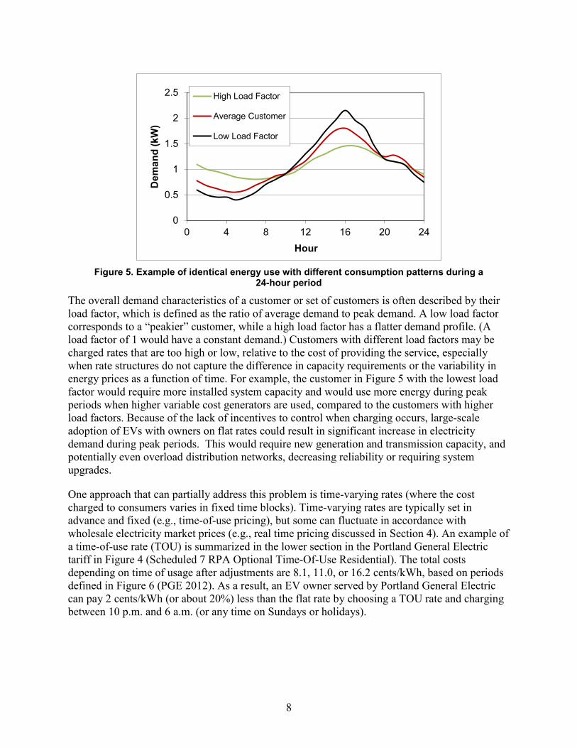
Figure 5. Example of identical energy use with different consumption patterns during a

24-hour period

The overall demand characteristics of a customer or set of customers is often described by their load factor, which is defined as the ratio of average demand to peak demand. A low load factor corresponds to a “peakier” customer, while a high load factor has a flatter demand profile. (A load factor of 1 would have a constant demand.) Customers with different load factors may be charged rates that are too high or low, relative to the cost of providing the service, especially when rate structures do not capture the difference in capacity requirements or the variability in energy prices as a function of time. For example, the customer in Figure 5 with the lowest load factor would require more installed system capacity and would use more energy during peak periods when higher variable cost generators are used, compared to the customers with higher load factors. Because of the lack of incentives to control when charging occurs, large-scale adoption of EVs with owners on flat rates could result in significant increase in electricity demand during peak periods. This would require new generation and transmission capacity, and potentially even overload distribution networks, decreasing reliability or requiring system upgrades.

One approach that can partially address this problem is time-varying rates (where the cost charged to consumers varies in fixed time blocks). Time-varying rates are typically set in advance and fixed (e.g., time-of-use pricing), but some can fluctuate in accordance with wholesale electricity market prices (e.g., real time pricing discussed in Section 4). An example of a time-of-use rate (TOU) is summarized in the lower section in the Portland General Electric tariff in Figure 4 (Scheduled 7 RPA Optional Time-Of-Use Residential). The total costs depending on time of usage after adjustments are 8.1, 11.0, or 16.2 cents/kWh, based on periods defined in Figure 6 (PGE 2012). As a result, an EV owner served by Portland General Electric can pay 2 cents/kWh (or about 20%) less than the flat rate by choosing a TOU rate and charging between 10 p.m. and 6 a.m. (or any time on Sundays or holidays).

0

0.5

1

1.5

2

2.5

0 4 8 12 16 20 24

Dem

and

(kW

)

Hour

High Load Factor

Average Customer

Low Load Factor

8

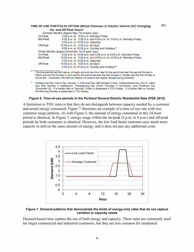
Figure 6. Time-of-use periods in the Portland General Electric Residential Rate (PGE 2012)

A limitation to TOU rates is that they do not distinguish between capacity needed by a customer and actual energy consumed. Figure 7 illustrates an example of a time-of-use rate with two customer usage patterns. As with Figure 5, the amount of energy consumed in this 24-hour period is identical. In Figure 7, energy usage within the on-peak (3 p.m. to 8 p.m.) and off-peak periods by both customers is identical. However, the low load factor customer uses much more capacity to deliver the same amount of energy, and it does not pay any additional costs.

Figure 7. Demand patterns that demonstrate the limits of energy-only rates that do not capture variation in capacity needs

Demand-based rates capture the use of both energy and capacity. These rates are commonly used for larger commercial and industrial customers, but they are less common for residential

00.5

11.5

22.5

33.5

44.5

0 4 8 12 16 20 24

Dem

and

(kW

)

Hour

Low Load Factor

Average Customer

9

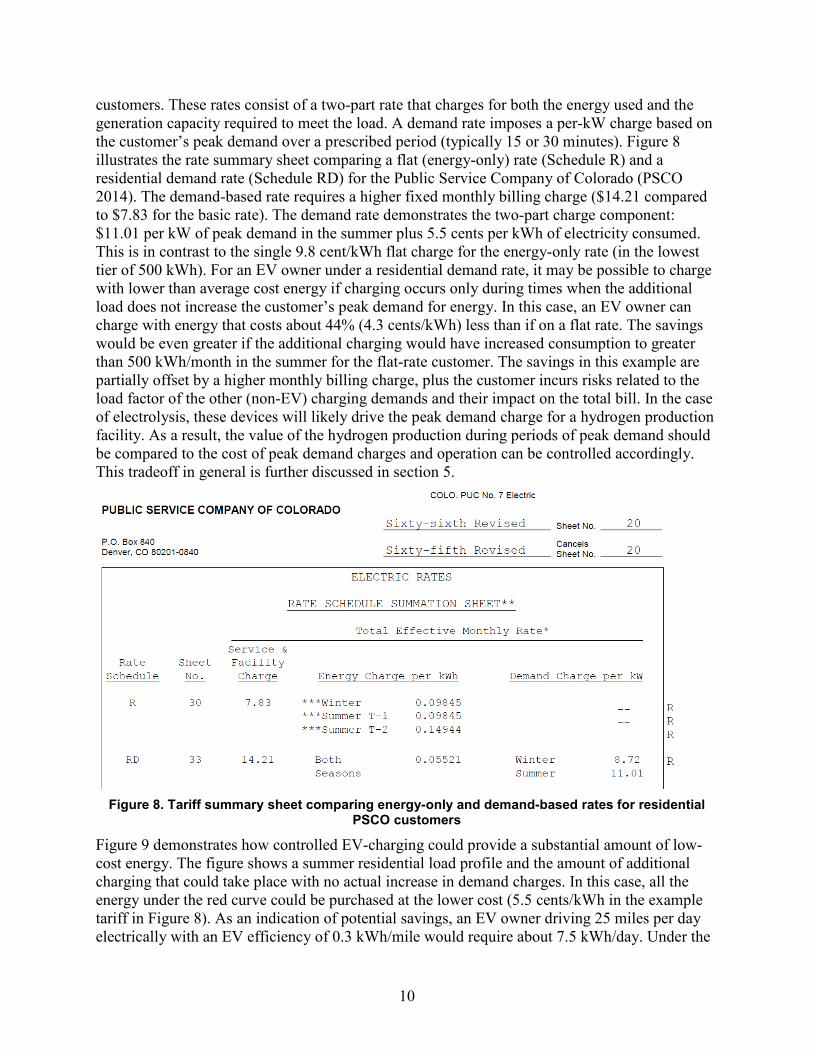
customers. These rates consist of a two-part rate that charges for both the energy used and the generation capacity required to meet the load. A demand rate imposes a per-kW charge based on the customer’s peak demand over a prescribed period (typically 15 or 30 minutes). Figure 8 illustrates the rate summary sheet comparing a flat (energy-only) rate (Schedule R) and a residential demand rate (Schedule RD) for the Public Service Company of Colorado (PSCO 2014). The demand-based rate requires a higher fixed monthly billing charge ($14.21 compared to $7.83 for the basic rate). The demand rate demonstrates the two-part charge component: $11.01 per kW of peak demand in the summer plus 5.5 cents per kWh of electricity consumed. This is in contrast to the single 9.8 cent/kWh flat charge for the energy-only rate (in the lowest tier of 500 kWh). For an EV owner under a residential demand rate, it may be possible to charge with lower than average cost energy if charging occurs only during times when the additional load does not increase the customer’s peak demand for energy. In this case, an EV owner can charge with energy that costs about 44% (4.3 cents/kWh) less than if on a flat rate. The savings would be even greater if the additional charging would have increased consumption to greater than 500 kWh/month in the summer for the flat-rate customer. The savings in this example are partially offset by a higher monthly billing charge, plus the customer incurs risks related to the load factor of the other (non-EV) charging demands and their impact on the total bill. In the case of electrolysis, these devices will likely drive the peak demand charge for a hydrogen production facility. As a result, the value of the hydrogen production during periods of peak demand should be compared to the cost of peak demand charges and operation can be controlled accordingly. This tradeoff in general is further discussed in section 5.

Figure 8. Tariff summary sheet comparing energy-only and demand-based rates for residential

PSCO customers

Figure 9 demonstrates how controlled EV-charging could provide a substantial amount of low-cost energy. The figure shows a summer residential load profile and the amount of additional charging that could take place with no actual increase in demand charges. In this case, all the energy under the red curve could be purchased at the lower cost (5.5 cents/kWh in the example tariff in Figure 8). As an indication of potential savings, an EV owner driving 25 miles per day electrically with an EV efficiency of 0.3 kWh/mile would require about 7.5 kWh/day. Under the

10

flat rate, this incremental energy would cost about 74 cents per day or about $22/month in the winter or lower summer tier, or $33/month in the higher summer tier. It is likely that EV charging at 7.5 kWh per day (225 kWh/month) would likely shift a typical customer to the higher tier in the summer, as this usage is nearly half the lower tier limit of 500 kWh/month. Under a demand rate, this energy would cost about 41 cents per day or about $12/month under all conditions. So, for a typical consumer, switching to a demand-based rate would save about $10/month in energy costs during the winter and $21/month in the summer, assuming the higher usage rate. This corresponds to a net savings of about $3/month in the winter or about $15/month in the summer after adding the additional $6.38/month in fixed billing charges associated with the demand-based rate. This assumes no other changes in demand patterns associated with switching to a demand-based rate. Of note in Figure 9 is the relatively limited charging rate, even in overnight, off-peak periods. The maximum rate in this example is only about 2.5 kW. While this would be sufficient to deliver the assumed average daily 7.5-kWh requirement—requiring only two kW for about four hours—a pure EV needing a full charge may require a higher charging capacity. A level 2 (240V) charger can typically deliver up to 6.6 kW and would likely drive peak demand, and it would negate most benefits from a demand-based rate. It is important to note that Figure 9 is illustrative only, with a relatively smooth load profile; it does not illustrate demand peaks that can occur from oven or air-conditioner use that can drive peak demand. However, it does illustrate that some level of intelligent charging may be needed to control peak demand, particularly in the winter, when peak demand may be lower.

Figure 9. Demand-based energy rates can offer low-cost energy for EV charging if appropriately timed. The red line shows a demand profile for EV charging that would not raise peak demand,

and hence the demand charges.

These examples demonstrate that individual EV owners must consider their flexibility of charging, and how this flexibility can help minimize costs given the potential availability of multiple rate structures. It should also be emphasized that there is tremendous variability across regions as to the types and availability of rates offered. For example, Figure 10 illustrates snapshots of three residential rate structures from Georgia Power: flat, time of use, and demand.5

5 See Georgia Power Residential Service Schedules: “R-20”, “TOU-RD-1” and “TOU-PEV-4” at www.georgiapower.com/pricing/files/rates-and-schedules/residential-rates/2.10_R-20.pdf,

00.5

11.5

22.5

33.5

4

0 4 8 12 16 20 24

Dem

and

(kW

)

Hour

Normal Demand

Energy-OnlyCharging Available

11

(These exclude the riders, which add about 3–4 cents/kWh depending on rate type). There are several items of note about the example in this figure. First, the flat rate is tiered with decreasing tiers in the winter and increasing tiers in the summer. Second, the demand-based rate does not have a higher fixed (“basic service”) charge, which was a major source of the relatively small value associated with shifting to demand-based rates in the PSCO example. Third, the time-of-use and demand-based rates both show significantly greater variation in range than the previous examples. So, compared to the PSCO example (Figure 8), moving from flat to demand-based rates for a mid-tier consumer could save about $8/month in the winter (compared to $3/month for PSCO) and about $17/month in the summer (compared to $15/month for PSCO). However, the demand charge is much higher, meaning even greater care must be taken to avoid charging during periods of peak demand. Alternatively, the consumer could switch to the TOU rate and see a similar savings and not be restricted by limiting demand, which would be particularly important during winter months when peak demand could be relatively low.

www.georgiapower.com/pricing/files/rates-and-schedules/residential-rates/2.40_TOU-RD-1.pdf, and www.georgiapower.com/pricing/files/rates-and-schedules/residential-rates/2.30_TOU-PEV-4.pdf.

12

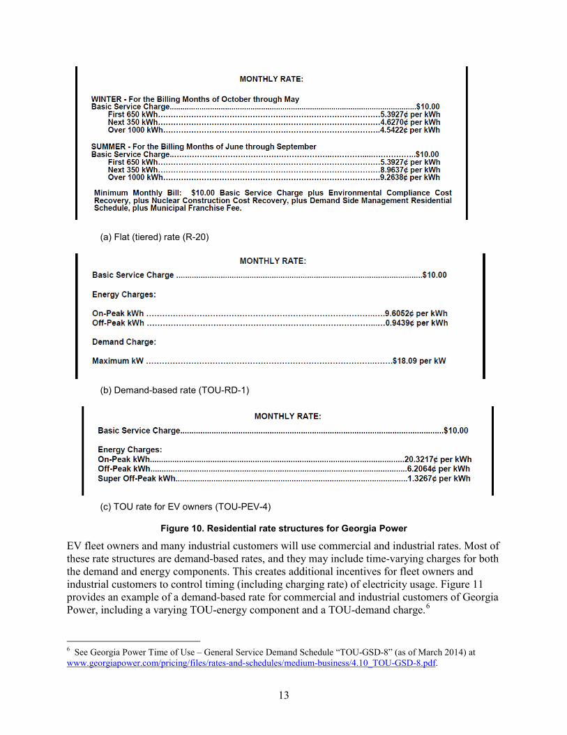
(a) Flat (tiered) rate (R-20)

(b) Demand-based rate (TOU-RD-1)

(c) TOU rate for EV owners (TOU-PEV-4)

Figure 10. Residential rate structures for Georgia Power

EV fleet owners and many industrial customers will use commercial and industrial rates. Most of these rate structures are demand-based rates, and they may include time-varying charges for both the demand and energy components. This creates additional incentives for fleet owners and industrial customers to control timing (including charging rate) of electricity usage. Figure 11 provides an example of a demand-based rate for commercial and industrial customers of Georgia Power, including a varying TOU-energy component and a TOU-demand charge.6

6 See Georgia Power Time of Use – General Service Demand Schedule “TOU-GSD-8” (as of March 2014) at www.georgiapower.com/pricing/files/rates-and-schedules/medium-business/4.10_TOU-GSD-8.pdf.

13

Figure 11. Rate TOU-GSD-8 for Georgia Power

Traditional LSE Demand Response and Interruptible Load Programs While time-of-use and demand-based rates allow for more accurate allocation of costs to different customers compared to energy-only rates, they still have limited ability to capture variation in system demand and costs that occur over various time intervals. This is illustrated by the hourly and season variation in system demand patterns that occur throughout the United States. Figure 12 provides the hourly demand for three weeks in the balancing area served by the Public Service Company of Colorado. Any small increase in demand by any individual customer during any period other than at 4 p.m. on July 7 would not have caused a need to build additional

14

generation capacity. (Additional loads may require additional distribution capacity depending on customer load shape, but they would not require new generation capacity.)

Figure 12. Hourly load profiles for the balancing area served by PSCO in 2003

Image generated by NREL using data derived from FERC 714 data.

Alternatively, had customers been incentivized to reduce demand at 4 p.m. on July 7, the utility could have potentially constructed less generation capacity and passed (at least part) of that savings to the customer who reduced demand. Especially if this generation is only required a few times a year, this potential for savings represents a primary motivation for current demand response programs. Figure 13 shows this potential savings based on the system’s load duration curve, or the hourly demand data sorted by load. The figure shows how many hours of the year a given amount of capacity is needed. Figure 13a shows the data for the entire year, while Figure 13b shows the data for the top 100 hours, showing that 200 MW of capacity is required for only 12 hours of the year or fewer, while 600 MW of capacity (about 10% of the total) is required for only 100 hours of the year or fewer.

05001,0001,5002,0002,5003,0003,5004,0004,5005,0005,5006,000

0.0

0.1

0.2

0.3

0.4

0.5

0.6

0.7

0.8

0.9

1.0

0 24 48 72 96 120 144 168

Load

(MW

)

Load

(Fra

ctio

n of

Ann

ual P

eak)

Hour & Day

Winter Spring Minimum

Summer Maximum

Annual system peak of 6228 MW, Wed July 7 at 4pm

15

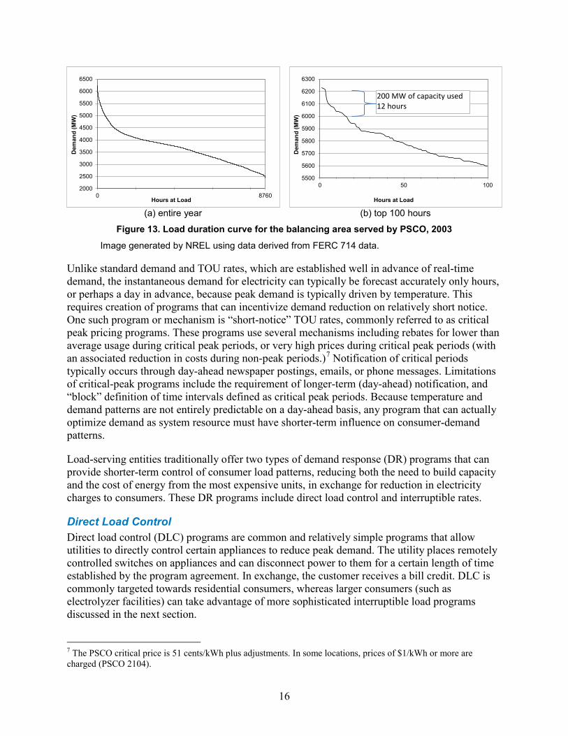
(a) entire year (b) top 100 hours

Figure 13. Load duration curve for the balancing area served by PSCO, 2003

Image generated by NREL using data derived from FERC 714 data.

Unlike standard demand and TOU rates, which are established well in advance of real-time demand, the instantaneous demand for electricity can typically be forecast accurately only hours, or perhaps a day in advance, because peak demand is typically driven by temperature. This requires creation of programs that can incentivize demand reduction on relatively short notice. One such program or mechanism is “short-notice” TOU rates, commonly referred to as critical peak pricing programs. These programs use several mechanisms including rebates for lower than average usage during critical peak periods, or very high prices during critical peak periods (with an associated reduction in costs during non-peak periods.)7 Notification of critical periods typically occurs through day-ahead newspaper postings, emails, or phone messages. Limitations of critical-peak programs include the requirement of longer-term (day-ahead) notification, and “block” definition of time intervals defined as critical peak periods. Because temperature and demand patterns are not entirely predictable on a day-ahead basis, any program that can actually optimize demand as system resource must have shorter-term influence on consumer-demand patterns.

Load-serving entities traditionally offer two types of demand response (DR) programs that can provide shorter-term control of consumer load patterns, reducing both the need to build capacity and the cost of energy from the most expensive units, in exchange for reduction in electricity charges to consumers. These DR programs include direct load control and interruptible rates.

Direct Load Control Direct load control (DLC) programs are common and relatively simple programs that allow utilities to directly control certain appliances to reduce peak demand. The utility places remotely controlled switches on appliances and can disconnect power to them for a certain length of time established by the program agreement. In exchange, the customer receives a bill credit. DLC is commonly targeted towards residential consumers, whereas larger consumers (such as electrolyzer facilities) can take advantage of more sophisticated interruptible load programs discussed in the next section.

7 The PSCO critical price is 51 cents/kWh plus adjustments. In some locations, prices of $1/kWh or more are charged (PSCO 2104).

2000

2500

3000

3500

4000

4500

5000

5500

6000

6500

0 8760

Dem

and

(MW

)

Hours at Load

5500

5600

5700

5800

5900

6000

6100

6200

6300

0 50 100

Dem

and

(MW

)

Hours at Load

200 MW of capacity used 12 hours

16

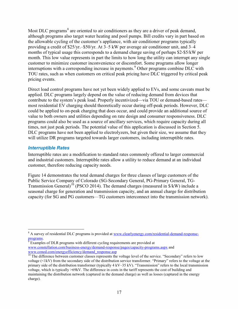
Most DLC programs8 are oriented to air conditioners as they are a driver of peak demand, although programs also target water heating and pool pumps. Bill credits vary in part based on the allowable cycling of the customer’s appliance, with air conditioner programs typically providing a credit of $25/yr.–$50/yr. At 3–5 kW per average air conditioner unit, and 3–4 months of typical usage this corresponds to a demand charge saving of perhaps $2-$5/kW per month. This low value represents in part the limits to how long the utility can interrupt any single customer to minimize customer inconvenience or discomfort. Some programs allow longer interruptions with a corresponding increase in payments.9 Other programs combine DLC with TOU rates, such as when customers on critical peak pricing have DLC triggered by critical peak pricing events.

Direct load control programs have not yet been widely applied to EVs, and some caveats must be applied. DLC programs largely depend on the value of reducing demand from devices that contribute to the system’s peak load. Properly incentivized—via TOU or demand-based rates—most residential EV charging should theoretically occur during off-peak periods. However, DLC could be applied to on-peak charging that does occur, and could provide an additional source of value to both owners and utilities depending on rate design and consumer responsiveness. DLC programs could also be used as a source of ancillary services, which require capacity during all times, not just peak periods. The potential value of this application is discussed in Section 5. DLC programs have not been applied to electrolyzers, but given their size, we assume that they will utilize DR programs targeted towards larger customers, including interruptible rates.

Interruptible Rates Interruptible rates are a modification to standard rates commonly offered to larger commercial and industrial customers. Interruptible rates allow a utility to reduce demand at an individual customer, therefore reducing capacity needs.

Figure 14 demonstrates the total demand charges for three classes of large customers of the Public Service Company of Colorado (SG-Secondary General, PG-Primary General, TG-Transmission General)10 (PSCO 2014). The demand charges (measured in $/kW) include a seasonal charge for generation and transmission capacity, and an annual charge for distribution capacity (for SG and PG customers—TG customers interconnect into the transmission network).

8 A survey of residential DLC programs is provided at www.clearlyenergy.com/residential-demand-response-programs. 9 Examples of DLR programs with different cycling requirements are provided at www.constellation.com/business-energy/demand-response/pages/capacity-programs.aspx and www.coned.com/energyefficiency/demand_response.asp 10 The difference between customer classes represents the voltage level of the service. “Secondary” refers to low voltage (<1kV) from the secondary side of the distribution service transformer. “Primary” refers to the voltage at the primary side of the distribution transformer (typically 4 kV–35 kV). “Transmission” refers to the local transmission voltage, which is typically >69kV. The difference in costs in the tariff represents the cost of building and maintaining the distribution network (captured in the demand charge) as well as losses (captured in the energy charge).

17

Figure 14. Tariff sheet summary for large customers of PSCO

Each of these customers may take an “Interruptible Service Option Credit” if they are able to shed more than 300 kW of demand. Figure 15 demonstrates components of this credit.11 The first component is the credit calculation, which involves in part the flexibility of the load (determined by the Capacity Availability factor - Ca). As shown in Figure 15, this combines the total annual hours of disruption (up to 40, 80, or 160 hours), and the length of duration within each 24-hour period (up to 4 hours or unconstrained). A highly flexible load that is willing to be interrupted with unlimited duration of individual interruptions up to a total of 160 hours per year would be credited at 95% of the $7.65 charge. This produces a demand charge reduction of $8.36 to $8.78 depending on system loss factor (determined by the delivery voltage), and excluding the additional small credit for the number of interruptible hours. This number is a substantial fraction of the total generation and transmission-related demand charge, which ranges from $14.04/kW to $16.00/kW depending on customer type. Overall, this means that interruptible rates can reduce the cost of generation and transmission related demand charges by as much as about 60%.

11 From Public Service Company of Colorado: Interruptible Service Option Credit Schedule ISOC, Sixth Revised Sheet 90E, issued December 20, 2013, and Fourth Revised Sheet 90C, issued December 16, 2008.

18

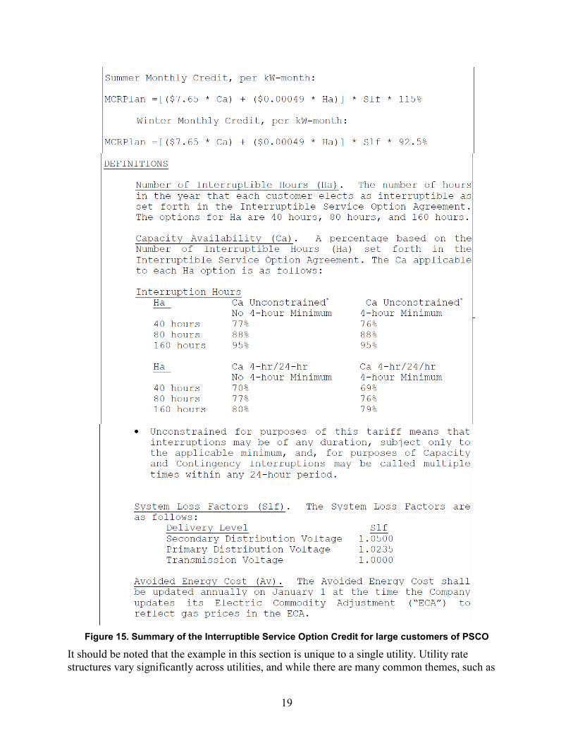
Figure 15. Summary of the Interruptible Service Option Credit for large customers of PSCO

It should be noted that the example in this section is unique to a single utility. Utility rate structures vary significantly across utilities, and while there are many common themes, such as

19

demand-based rates for larger customers, each tariff needs to be examined thoroughly for details unique to each LSE.

Limitations of Rate Structures for Optimized EV Charging and Electrolyzer Use

The examples provided in this section indicate that EV and electrolyzer owners have multiple options to minimize costs in standard rate structures. The most critical factor is likely the availability of demand-based rates so that charging can occur with only the energy (variable) component of electricity costs. While they are common for larger customers, demand-based rates are less common for residential customers. This leaves residential customers with TOU rates as the primary option to control costs. Given the flexibility of EV charging and electrolyzer production, a secondary mechanism to minimize capacity-related costs is likely desirable. Industrial customers have this option with interruptible loads, but new mechanisms may be important for smaller customers. This could include modification to existing rate structures that allow for direct load control of EVs and electrolyzers to minimize on-peak charging.

From the utility perspective, proper incentives will likely be needed to ensure that large-scale deployment of EVs does not increase the need for new generation, transmission, or distribution capacity. Previous analysis has demonstrated that significant EV deployment can provide system benefits when charging can be controlled, but also have significant negative impacts if not controlled (Sioshansi and Denholm 2010). New mechanism may be particularly important when controlled charging is used to help integrate variable generation resources such as solar and wind (Denholm et al. 2013). Standard rate structures are somewhat limited in their ability to allow customers to respond to the real variability in energy price, capacity requirements, and need for ancillary services. Wholesale market-based transactions have the ability to address some of these issues, as discussed in the following sections.

20

4 Wholesale Market-Based Energy Transactions The creation of restructured wholesale markets allows several alternative mechanisms for consumers to purchase and sell electricity services. Wholesale markets are operated by an independent system operator (ISO) or regional transmission operator (RTO). Figure 16 shows U.S. locations with restructured markets, which together cover about two-thirds of U.S. electricity demand.12 Larger industrial customers in these regions can interact directly with the wholesale energy market to acquire capacity and energy. Smaller retail customers can also interact with the market through a load-serving entity or aggregator.

Figure 16. Locations with restructured markets

Source: FERC (http://www.ferc.gov/industries/electric/indus-act/rto.asp)

Market-based energy purchases allow for the greatest level of control over the timing and costs of energy purchases. Large industrial customers can purchase energy directly from suppliers either bilaterally in all parts of the United States or from RTO/ISO markets where they exist. Smaller customers have fewer options; however, some LSEs offer real-time prices, where the prices are based on conditions in the wholesale market.

For small customers using a real-time pricing mechanism, or for industrial customers that employ direct market purchases but still use a local distribution system owned by a regulated distribution company, there will be essentially two separate bills. The first is from the regulated distribution company, which covers the cost of building and maintaining the distribution network. An example of a distribution-only bill for Ameren Illinois is shown in Figure 17. Illinois offers electricity customer choice, and this example includes rates for both residential customers (Schedule DS-1) and large customers (Schedule DS-3).13 Note that in this example the

12 ISO/RTO Council (www.isorto.org/about/default) 13 www.ameren.com/-/media/Illinois-Site/Files/rates/aiifMAPP115.pdf?la=en

21

distribution charge for residential customers is on a volumetric basis, meaning that off-peak charging will incur an additional cost, even if the charging does not actually increase demand on the distribution network. The charge for large customers is a demand-based rate.

Figure 17. Example of distribution-only tariffs for customers that take energy from a competitive

energy supplier

The energy portion of real-time prices includes multiple components—depending on how the real time pricing program is implemented—including capacity, transmission use, ancillary

22

services, and the variable components of energy supply (largely reflected in the real time price of energy from the market). Energy represents the electrical energy (measured in kWh or MWh). Capacity represents the physical capability to deliver energy to the consumer. It includes generation capacity, transmission, and distribution infrastructure, and it is measured in kW or MW. Ancillary services represent a broad array of services that help system operators maintain a reliable grid with sufficient power quality, including such services as operating reserves. While ancillary services are a relatively small fraction of the total system operating costs—on the order of 1%–2% of the total (Kirby and Hirst 1996, Hummon et al. 2013)—they represent an important potential source of revenue for suppliers. Ancillary services are discussed in detail in Section 5.

The capacity component is similar to a demand charge, except the demand may be based both on usage in a previous year and on a fixed interval.14 This charge is substantially different from typical demand-based rates, which may use peak demand at any point in time or during a fixed daily window over a season.

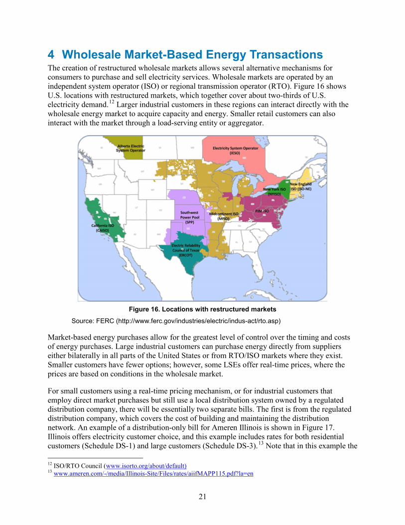
The energy component of real-time prices are based on the market clearing prices of the relevant market, which will have adjustments applied for factors such as the higher loss rates associated with residential customers. Figure 18 provides the average hourly price for electricity in the PJM market during three seasons in 2012. It demonstrates significantly lower prices during off-peak periods, which generally follow the patterns in conventional rate structures discussed in Section 3.

14 Commonwealth Edison (ComEd) describes the calculation as follows: “If you were enrolled in the RRTP [real-time pricing program] program or had a smart meter during the previous summer, your Capacity Obligation is based on your individual electricity usage data from that summer. In this case, ComEd calculates your highest electricity demand (adjusted for Transmission and Distribution losses) coincident with the five hours of the summer when the overall PJM System demand was highest (PJM Coincident Demand) (this has historically occurred between 1 p.m. and 5 p.m. on weekdays), and the five hours of the summer when ComEd’s System demand was highest (ComEd Coincident Demand) (these sets of hours may or may not overlap). These two sets of five coincident demands are averaged and adjusted to determine your contribution to the system load, creating your Capacity Obligation.” (ComEd 2014)

23

Figure 18. Seasonal price patterns for the PJM market in 2012

Overall, real-time prices for smaller customers are still relatively rare, and they can be very complex.15 However, they also provide the greatest flexibility for small consumers to optimize charging during periods of absolute lowest cost. This even provides an opportunity for residential customers to be exposed to negative electricity prices.16 This comes at the additional complexity of needing to monitor constant variation in prices, although automation can reduce the burden.

As discussed above, large industrial customer may purchase energy directly from the market, including independent power producers or the market operator, and they can include some combination of long-term bilateral contracts, as well as purchases from the day-ahead or real-time markets. Regardless of mechanisms, the ability to control the timing of use provides significant flexibility to minimize energy costs. Avoiding electricity use during periods of high prices can minimize total costs; this comes at a tradeoff with overall utilization. Figure 19 compares the average and marginal price as a function of capacity factor. For example, a plant operating during only 20% of all hours of the year would have paid on average about $21/MWh, while one operating at 80% would pay about $29/MWh.

15 For example, the Ameren Real-Time Pricing Program requires multiple riders with complicated formulas for the multiple components of energy and capacity. See www.ameren.com/-/media/illinois-site/Files/Rates/AIel27rdrtp.pdf. 16 From “The ComEd Residential Real-Time Pricing Program Guide to Real-Time Pricing” - “With real-time hourly market prices, it is possible for the price of electricity to be negative for short periods of time. This typically occurs in the middle of the night and, under certain circumstances, when electricity supply is far greater than demand. In the market, some types of electricity generators cannot or prefer not to reduce electricity output for short periods of time when demand is insufficient, and as a result some generators may provide electricity to the market at prices below zero. Since ComEd RRTP participants pay the market price of electricity, they are actually being paid to use electricity during negative priced hours” https://rrtp.comed.com/wp-content/uploads/2014/09/RRTPGuide2014-06-final.pdf

0

10

20

30

40

50

60

70

0 6 12 18 24

Loca

tiona

l Mar

gina

l Pric

e ($

/MW

h)

Winter

Summer

Spring

24

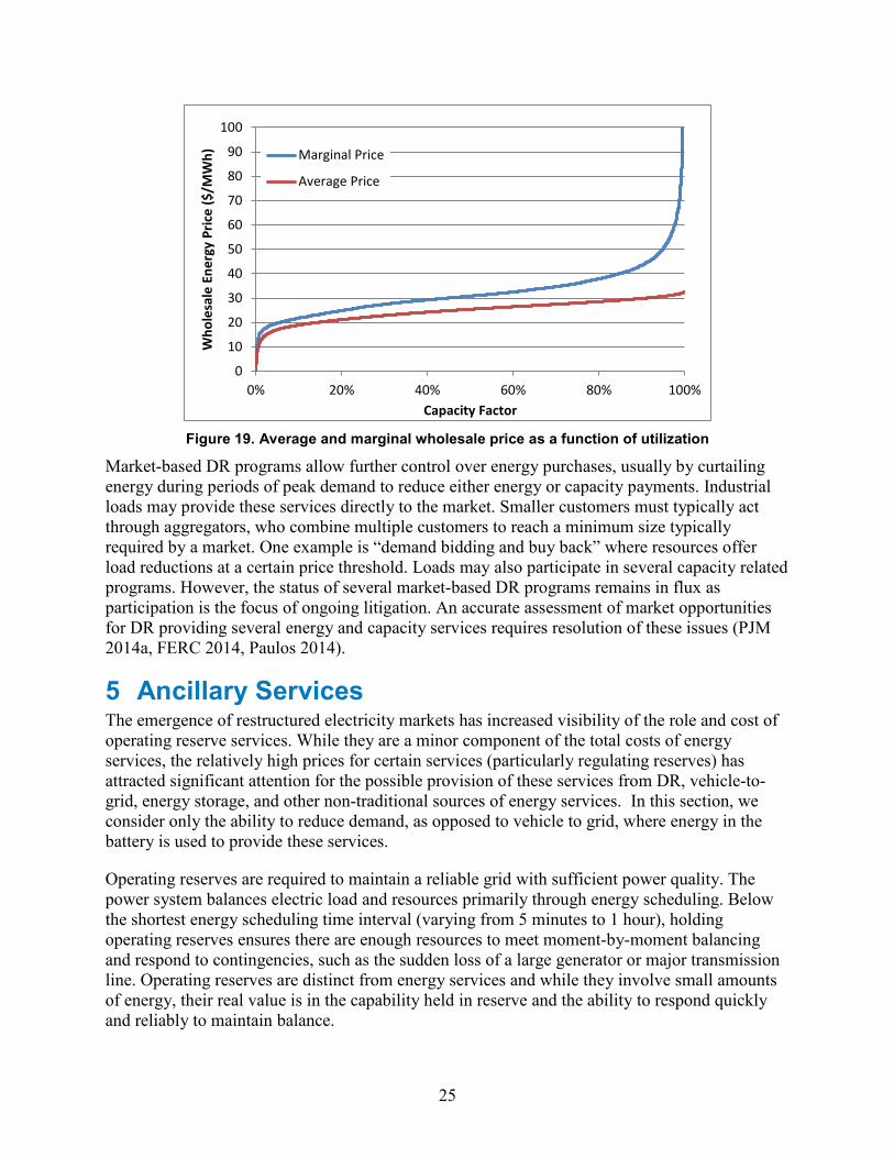
Figure 19. Average and marginal wholesale price as a function of utilization

Market-based DR programs allow further control over energy purchases, usually by curtailing energy during periods of peak demand to reduce either energy or capacity payments. Industrial loads may provide these services directly to the market. Smaller customers must typically act through aggregators, who combine multiple customers to reach a minimum size typically required by a market. One example is “demand bidding and buy back” where resources offer load reductions at a certain price threshold. Loads may also participate in several capacity related programs. However, the status of several market-based DR programs remains in flux as participation is the focus of ongoing litigation. An accurate assessment of market opportunities for DR providing several energy and capacity services requires resolution of these issues (PJM 2014a, FERC 2014, Paulos 2014).

5 Ancillary Services The emergence of restructured electricity markets has increased visibility of the role and cost of operating reserve services. While they are a minor component of the total costs of energy services, the relatively high prices for certain services (particularly regulating reserves) has attracted significant attention for the possible provision of these services from DR, vehicle-to-grid, energy storage, and other non-traditional sources of energy services. In this section, we consider only the ability to reduce demand, as opposed to vehicle to grid, where energy in the battery is used to provide these services.

Operating reserves are required to maintain a reliable grid with sufficient power quality. The power system balances electric load and resources primarily through energy scheduling. Below the shortest energy scheduling time interval (varying from 5 minutes to 1 hour), holding operating reserves ensures there are enough resources to meet moment-by-moment balancing and respond to contingencies, such as the sudden loss of a large generator or major transmission line. Operating reserves are distinct from energy services and while they involve small amounts of energy, their real value is in the capability held in reserve and the ability to respond quickly and reliably to maintain balance.

0

10

20

30

40

50

60

70

80

90

100

0% 20% 40% 60% 80% 100%

Who

lesa

le E

nerg

y Pr

ice

($/M

Wh)

Capacity Factor

Marginal Price

Average Price

25

The nomenclature and technical requirements for various reserves services varies significantly across market regions. We consider three different operating reserves products that are maintained in some form, across all balancing authority areas in the United States, listed below.17

• Regulating reserves also known as are frequency regulation are held and dispatched to meet relatively small and random variations around normal load patterns.

• Contingency reserves are held to meet unplanned generation or transmission outage and must respond rapidly to sudden but infrequent supply disruptions)

• Non-spinning/replacement/supplemental reserves are held to address longer-term events and contingencies

Technical Requirements The technical requirements (and often the name) of each reserve product varies by market. Because operating reserves are traditionally provided by conventional generators, their technical requirements have been historically defined in the context of generators; however, the requirements are evolving to consider demand response and other technologies that have capabilities that differ from conventional generation. Key parameters that qualify a resource to be able to provide operating reserves include:

• Synchronization—describes whether a generator needs to be synchronized (spinning) to provide the service

• Response rate—describes how long it takes a device to begin responding and how long it takes to fully respond

• Response duration—how long a device must maintain the response. Regulating reserves, when provided by conventional generation, requires generation that is synchronized and able to begin responding upon receipt of the automatic generation control signal. The North American Electric Reliability Corporation (NERC) requires the control signal be refreshed no less frequently than every six seconds. The response rate requirement, or time to achieve full output varies by location and can be 5 to 15 minutes (Ela et al. 2011). Regulation is required to respond to both increases and decreases in demand. Some regions combine their upward and downward reserve while others have separated requirements. Combined requirements imply that the upward and downward requirements must be equal and any resource providing upward reserve must be able to provide the same amount of downward reserve. Regions with separate services can have different requirements and can have different resources providing different amounts of upward and downward reserve. This represents an important distinction for provision of regulating reserves from DR. A device consuming energy at maximum capacity can provide upward reserves (by reducing demand) but can provide no downward reserves. Likewise, an idle device can provide downward reserves by increasing energy consumption, but cannot provide upward reserves. Furthermore, in the case of a fully

17 For additional discussion of terms applied to various reserve products, see the NERC Glossary of Terms Used in NERC Reliability Standards (www.nerc.com/files/Glossary_of_Terms.pdf) and Ela et al. (2011).

26

charged EV, which is not charging and cannot accept further charge, it cannot provide either upward or downward reserves.

Contingency reserves include spinning and non-spinning components, but many regions require a minimum percentage to be spinning (e.g., 50% for balancing authorities under the Western Electricity Coordinating Council (NERC 2008) and 40% in the Mid-Continent ISO (MISO) (2013)). The spinning component of contingency reserves requires synchronization, and it typically requires full response in 15 minutes or less (ten minutes is a common response rate requirement.) Response duration varies. NERC standard BAL-002 (DCS) states that the contingency reserve should be restored 90 minutes following the start of the restoration period. However, most contingencies are restored much faster (often less than 10 minutes), and actual response duration varies by balancing authority. For example, the Western Electricity Coordinating Council (WECC) requires that reserves be restored no later than 60 minutes following a disturbance event, and the New York Independent System Operator (NYISO) requires restoration of its 10-minute spinning reserve product within 30 minutes.

Non-spinning reserves are the least technically demanding service, typically being provided by fast-start generators that can normally start within 10 minutes. However, actual response rate varies by region (e.g., ERCOT requires full response in 30 minutes).

Cost There are two sources of the cost of operating reserves: fixed (capacity) and variable (operating) costs. Fixed costs represent the need to build capacity to meet reserve requirements. Variable costs are imposed by the need to keep a subset of generators operating at part load, available to increase output if needed. From the perspective of an individual generator, keeping a unit at part load incurs an opportunity cost because it cannot be dispatched to its full output. From the system perspective, the need for reserves can result in higher generation costs because keeping plants at part load increases the number of plants that are online. These additional online units have equal or higher production costs than the generators that were backed down to provide reserves. This ultimately results in higher operational costs (more fuel use and more units started) per unit of energy actually produced. In addition, partial loading can reduce the efficiency of individual power plants, particularly when plants are providing regulation reserve, which requires continuous changes in output over short periods. Non-steady state operation resulting from providing regulation reserves can also increase operations and maintenance requirements (Kumar et al. 2012). Hummon et al. (2013) provide an extensive discussion of the origin of reserves costs.

In non-ISO/RTO balancing authority areas, transmission providers charge their transmission customers for operating reserves that they do not self-supply or procure through third-party supply (FERC, 2013). Operating reserves are typically quoted on a monthly basis, and costs are generally settled according to the transmission customers’ contribution to the transmission system peak load (see Table 1).

27

Table 1. Selected Ancillary Service Tariffs in Non-ISO/RTO Balancing Authority Areas (Ma et al. 2013)

Tariff ($/kW-month)

Balancing Authority Regulation Spinning Contingency

American Electric Power, West Zone 2.64 3.56

Arizona Public Service 7.41 6.26

Duke Energy, Carolina Power & Light 3.96 3.96

El Paso Electric 3.10 3.10

Florida Power & Light 4.82 5.16

Idaho Power 6.53 6.53

PacifiCorp West 7.80 8.80

Portland Gas & Electric 6.70 6.45

Public Service of Colorado 6.74 6.88

Public Service of New Mexico 8.60 9.36

Southern Company 4.20 4.20

Tucson Electric 12.1 12.09 Where there is an organized wholesale market, the ISO/RTO balancing authority runs a competitive market for the supply of operating reserves. Historical operating reserve prices are available from ISO/RTO websites. The cost of regulating reserve is the combination of the opportunity cost calculated by the system operator and the bid cost, which represents the impact of non-steady-state operation, including increased operations and maintenance and heat rate effects from unit movement.

Table 2 shows significant variation between regions, but several commonalities emerge. First, many markets show significant year-to-year variation in the price, typically more than can be explained by underlying factors such as variation in natural gas prices. A second common theme is that the value of regulation is substantially higher than spin, with a clearing price often twice that of spinning reserves, as shown in Figure 20.

28

Table 2. Selected Ancillary Service Prices in Several ISO/RTO Markets, 2002–2012a

Average Market Clearing Price $/MW-hour Operating Reserve 2002 2003 2004 2005 2006 2007 2008 2009 2010 2011 2012 California ISO Regulation (Up + Down)

26.9 35.5 28.7 35.2 38.5 26.1 33.4 12.6 10.6 16.1 10.0

Spinning 4.3 6.4 7.9 9.9 8.4 4.5 6.0 3.9 4.1 7.2 3.3 Non-spinning 1.8 3.6 4.7 3.2 2.5 2.8 1.3 1.4 0.6 1.0 0.9 Replacement 0.90 2.9 2.5 1.9 1.5 2.0 1.4 Electric Reliability Council of Texas Regulation (Up + Down)

16.9 22.6 38.6 25.2 21.4 43.1 17.0 18.1 31.3 9.2

Responsive 7.3 8.3 16.6 14.6 12.6 27.2 10.0 9.1 22.9 9.1 Non-Spin 3.2 1.9 6.1 4.2 3.0 4.4 2.3 4.3 11.8 6.7 New York ISO (east) Regulation 18.6 28.3 22.6 39.6 55.7 56.3 59.5 37.2 28.8 11.8 10.4 Spinning 3.0 4.3 2.4 7.6 8.4 6.8 10.1 5.1 6.2 7.4 6.0 Non-spinning 1.5 1.0 0.3 1.5 2.3 2.7 3.1 2.5 2.3 3.9 3.8 30 Minute 1.2 1.0 0.3 0.4 0.6 0.9 1.1 0.5 0.1 0.1 0.3 Midwest ISO (day ahead) Regulation 12.3 12.2 10.8 7.8 Spinning 4.0 4.0 2.8 2.3 Non-spinning 0.3 1.5 1.2 1.4 ISO New England Regulation + mileage 54.6 30.2 22.7 12.7 13.8 9.3 7.1 7.2 6.7 Spinning 0.3 0.4 1.7 0.7 1.8 1.0 1.7 10 Minute 0.1 0.3 1.2 0.5 1.6 0.4 1.0 30 Minute 0.0 0.1 0.1 0.1 0.4 0.3 1.0

a Contingency reserve, as described in the text, is sometimes called spinning and non-spinning reserve, responsive reserve, or 10-minute and 30-minute reserve. (Milligan & Kirby, 2010), updated.

29

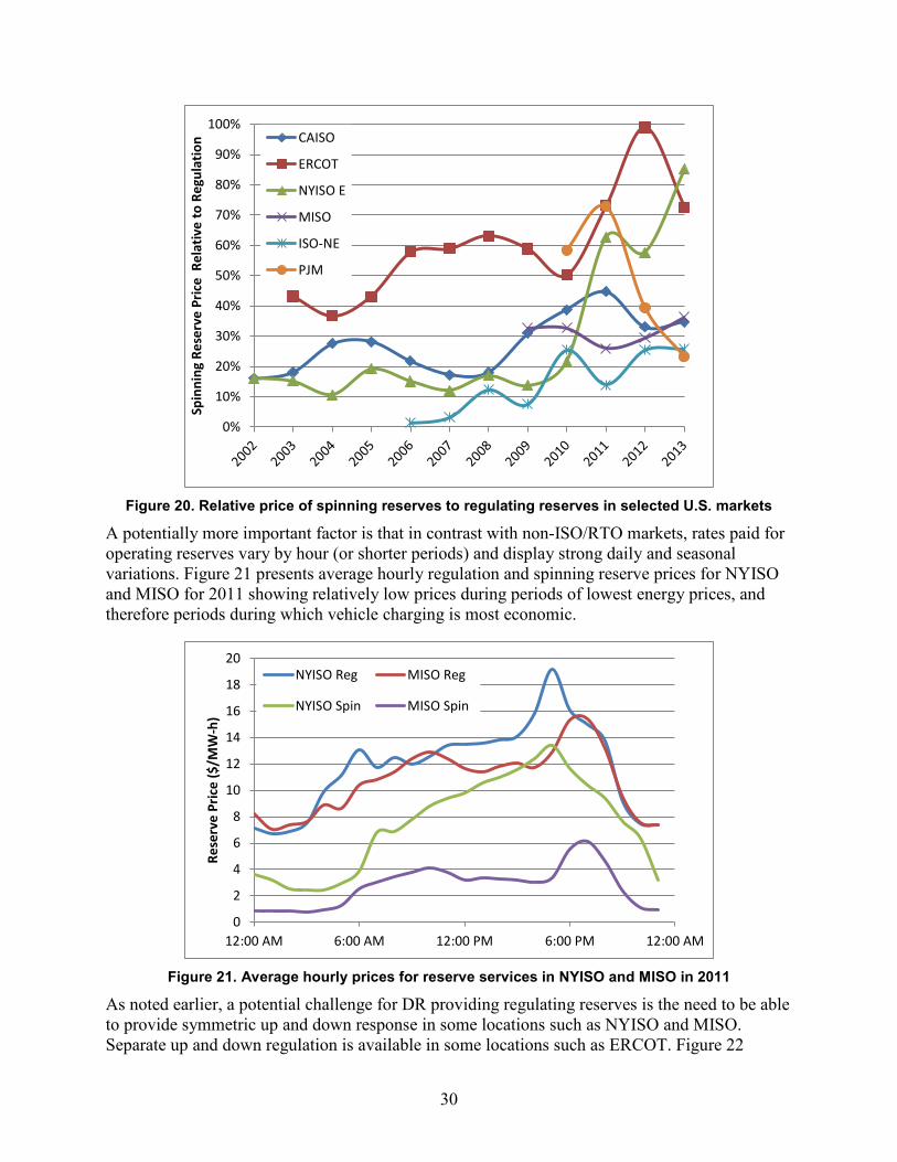
Figure 20. Relative price of spinning reserves to regulating reserves in selected U.S. markets

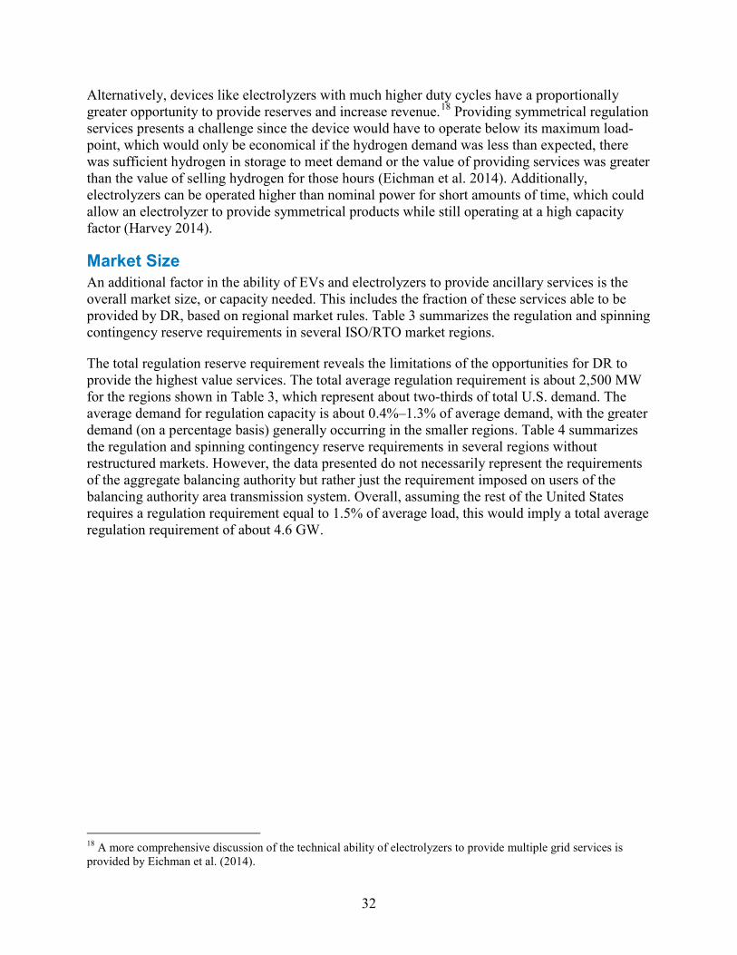
A potentially more important factor is that in contrast with non-ISO/RTO markets, rates paid for operating reserves vary by hour (or shorter periods) and display strong daily and seasonal variations. Figure 21 presents average hourly regulation and spinning reserve prices for NYISO and MISO for 2011 showing relatively low prices during periods of lowest energy prices, and therefore periods during which vehicle charging is most economic.

Figure 21. Average hourly prices for reserve services in NYISO and MISO in 2011

As noted earlier, a potential challenge for DR providing regulating reserves is the need to be able to provide symmetric up and down response in some locations such as NYISO and MISO. Separate up and down regulation is available in some locations such as ERCOT. Figure 22

0%

10%

20%

30%

40%

50%

60%

70%

80%

90%

100%

Spin

ning

Res

erve

Pric

e R

elat

ive

to R

egul

atio

n CAISO

ERCOT

NYISO E

MISO

ISO-NE

PJM

0

2

4

6

8

10

12

14

16

18

20

12:00 AM 6:00 AM 12:00 PM 6:00 PM 12:00 AM

Rese

rve

Pric

e ($

/MW

-h)

NYISO Reg MISO Reg

NYISO Spin MISO Spin

30

provides the average hourly price for regulation up and down in ERCOT in 2012. To provide regulation up, a device must be consuming energy and must be able to reduce output. As with the data in Figure 21, this demonstrates that to provide regulation up, a DR device must be consuming energy in hours with relatively high price (either paying high demand charges on a tariff or paying high market prices from a restructured market). Alternatively, the provision of regulation down means the device must be able to increase demand. However, the highest prices for regulation down typically occur in the overnight periods of lowest energy costs, precisely when EV charging should be maximized and therefore cannot by increased to provide regulation down.

Figure 22. Average hourly regulation up and down prices for ERCOT in 2012

Overall, historic reserve prices indicate a low value for individual vehicle charging-only DR services during off-peak periods. A vehicle consuming 7.5 kWh per day will be able to provide 7.5 kW-hr of upward reserves per day while charging (where up reserves require reduction in demand). This provision is independent of charge rate (the vehicle could charge at 7.5 kW, providing 7.5 kw of “up” reserves for 1 hour or could charge at 1 kW, providing 1 kW of “up” reserves for 7.5 hours). This would provide about 2.74 MW-hr/year of reserves. However, for regulation services that require symmetrical response, the vehicle would need to charge at half rate. Assuming the vehicle were charging at half its maximum rate and could provide both up and down reserve at $7/MW-hr, (which is among the highest prices for off-peak services), this corresponds to about $26/year. This value would be likely be reduced by the cost of enabling communications for the vehicle to receive an AGC signal, validation, and any aggregator costs. Furthermore, provision of down reserves (meaning the vehicle increases charging) could require an increase in demand that would increase demand charges. Less complicated communication is needed for provision of spinning reserves but with corresponding lower value—probably under $15/year—assuming the same charging requirements and an off-peak spinning reserve price of <$4/MW-hr.

0

5

10

15

20

25

30

35

40

45

50

12:00 AM 4:00 AM 8:00 AM 12:00 PM 4:00 PM 8:00 PM 12:00 AM

Regu

latin

g Re

serv

e Pr

ice

($/M

W-h

) REGDN

REGUP

31

Alternatively, devices like electrolyzers with much higher duty cycles have a proportionally greater opportunity to provide reserves and increase revenue.18 Providing symmetrical regulation services presents a challenge since the device would have to operate below its maximum load-point, which would only be economical if the hydrogen demand was less than expected, there was sufficient hydrogen in storage to meet demand or the value of providing services was greater than the value of selling hydrogen for those hours (Eichman et al. 2014). Additionally, electrolyzers can be operated higher than nominal power for short amounts of time, which could allow an electrolyzer to provide symmetrical products while still operating at a high capacity factor (Harvey 2014).

Market Size An additional factor in the ability of EVs and electrolyzers to provide ancillary services is the overall market size, or capacity needed. This includes the fraction of these services able to be provided by DR, based on regional market rules. Table 3 summarizes the regulation and spinning contingency reserve requirements in several ISO/RTO market regions.

The total regulation reserve requirement reveals the limitations of the opportunities for DR to provide the highest value services. The total average regulation requirement is about 2,500 MW for the regions shown in Table 3, which represent about two-thirds of total U.S. demand. The average demand for regulation capacity is about 0.4%–1.3% of average demand, with the greater demand (on a percentage basis) generally occurring in the smaller regions. Table 4 summarizes the regulation and spinning contingency reserve requirements in several regions without restructured markets. However, the data presented do not necessarily represent the requirements of the aggregate balancing authority but rather just the requirement imposed on users of the balancing authority area transmission system. Overall, assuming the rest of the United States requires a regulation requirement equal to 1.5% of average load, this would imply a total average regulation requirement of about 4.6 GW.

18 A more comprehensive discussion of the technical ability of electrolyzers to provide multiple grid services is provided by Eichman et al. (2014).

32

Table 3. Regulation and Spinning Contingency Reserve Requirements in U.S. Wholesale Markets

Regulation Requirement Spinning Contingency Reserve 2013 Demand

CAISOa average (varies): ~338 MW up, ~325 MW down ~850 MW (average) peak: 45,097 MW average: 26,461 MW total: 231,800 GWH

ERCOTb average (varies): ~ 300 MW down, ~500 MW up range: 400–900 MW

2,800 MW (maximum of 50% from load) peak: 67,245 MW total: 332,000 GWH

MISOc range: 300–500 MW 1,000 MW (2,000 MW total and 1,000 MW of spin) peak: 98,576 MW average: 52,809 MW

PJMd average: 753 MW in 2013e

1,375 MW (Tier 2; maximum of 33% from DR)f peak: 157,508 MW total: 784,515 GWH

ISO-NEg average 60 MW range 30–150 MW

10-minute reserve: 1,750 MW 30-minute reserve: 2,430 MW

peak: 27,400 MW average: 14,900 MW

NYISOh 150–250 MW 10-minute spin: (330 east zone, 655 MW NY control area 10-minute total 1,310 MW

peak: 33,956 MW average: 18,700 MW

SPPi average: ~300 MW up, ~320 MW down 545 MW peak: 45.256 MW total: 230,879 GWh

a Reserves data are from CAISO (2013, p. 143). b All data are from Potomac Economics (2014, pp. 32, 97, and Xiii). c Reserves data are from Navid (2013, slides 4 and 5). Demand data are from MISO (2014, p. 15). d Except where noted, data are from Monitoring Analytics (2013) and Monitoring Analytics (2014). e Data are down from 943 MW in 2012 (Monitoring Analytics 2014, p. 3.) In the first 9 months of 2014, data from PJM indicate an average of 664 MW with a range of 525 MW to 700 MW. f All data are from PJM (2014b, p. 74). g All data are from Patton et al. (2014a, pp. 20, 46, 66, and 81). h All data are from Patton et al. (2014b, pp. a-21, 1–132, page iv.) i Reserves data are from www.spp.org/publications/Reserve%20Selection%20IDT%2020140121.pdf. Demand data are from SPP (2014, p. 21).

33

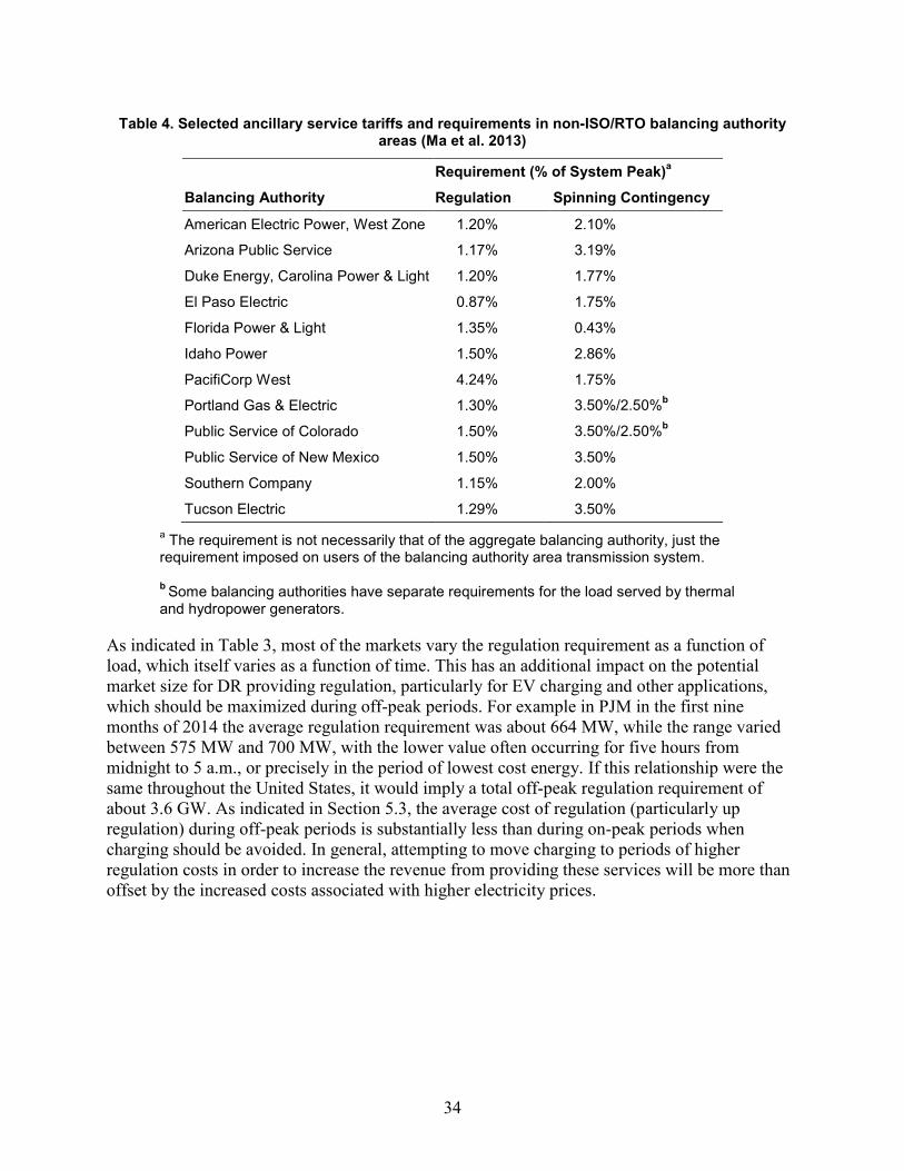
Table 4. Selected ancillary service tariffs and requirements in non-ISO/RTO balancing authority areas (Ma et al. 2013)

Requirement (% of System Peak)a

Balancing Authority Regulation Spinning Contingency

American Electric Power, West Zone 1.20% 2.10%

Arizona Public Service 1.17% 3.19%

Duke Energy, Carolina Power & Light 1.20% 1.77%

El Paso Electric 0.87% 1.75%

Florida Power & Light 1.35% 0.43%

Idaho Power 1.50% 2.86%

PacifiCorp West 4.24% 1.75%

Portland Gas & Electric 1.30% 3.50%/2.50%b

Public Service of Colorado 1.50% 3.50%/2.50%b

Public Service of New Mexico 1.50% 3.50%

Southern Company 1.15% 2.00%

Tucson Electric 1.29% 3.50% a The requirement is not necessarily that of the aggregate balancing authority, just the requirement imposed on users of the balancing authority area transmission system.

b Some balancing authorities have separate requirements for the load served by thermal and hydropower generators.

As indicated in Table 3, most of the markets vary the regulation requirement as a function of load, which itself varies as a function of time. This has an additional impact on the potential market size for DR providing regulation, particularly for EV charging and other applications, which should be maximized during off-peak periods. For example in PJM in the first nine months of 2014 the average regulation requirement was about 664 MW, while the range varied between 575 MW and 700 MW, with the lower value often occurring for five hours from midnight to 5 a.m., or precisely in the period of lowest cost energy. If this relationship were the same throughout the United States, it would imply a total off-peak regulation requirement of about 3.6 GW. As indicated in Section 5.3, the average cost of regulation (particularly up regulation) during off-peak periods is substantially less than during on-peak periods when charging should be avoided. In general, attempting to move charging to periods of higher regulation costs in order to increase the revenue from providing these services will be more than offset by the increased costs associated with higher electricity prices.

34

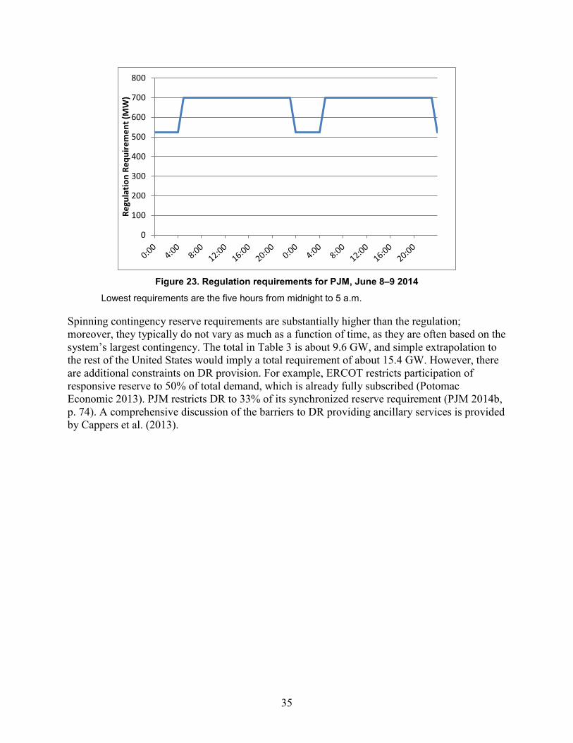
Figure 23. Regulation requirements for PJM, June 8–9 2014

Lowest requirements are the five hours from midnight to 5 a.m.

Spinning contingency reserve requirements are substantially higher than the regulation; moreover, they typically do not vary as much as a function of time, as they are often based on the system’s largest contingency. The total in Table 3 is about 9.6 GW, and simple extrapolation to the rest of the United States would imply a total requirement of about 15.4 GW. However, there are additional constraints on DR provision. For example, ERCOT restricts participation of responsive reserve to 50% of total demand, which is already fully subscribed (Potomac Economic 2013). PJM restricts DR to 33% of its synchronized reserve requirement (PJM 2014b, p. 74). A comprehensive discussion of the barriers to DR providing ancillary services is provided by Cappers et al. (2013).

0

100

200

300

400

500

600

700

800

Regu

latio

n Re

quire

men

t (M

W)

35

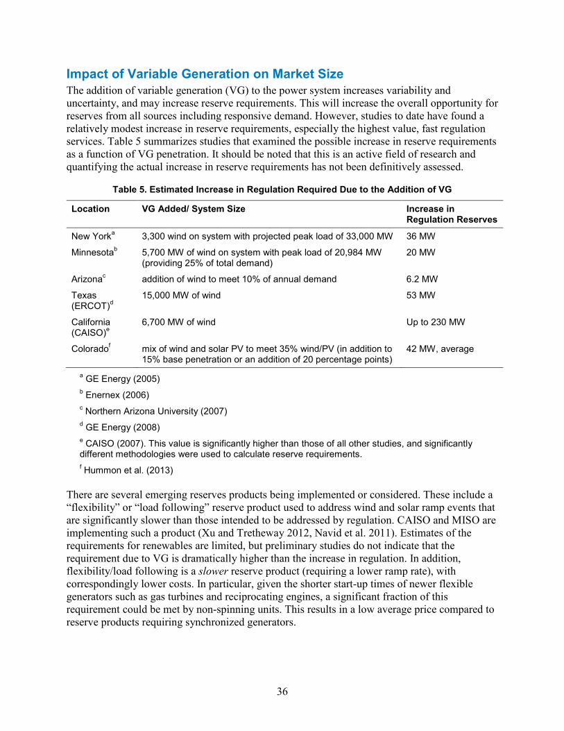
Impact of Variable Generation on Market Size The addition of variable generation (VG) to the power system increases variability and uncertainty, and may increase reserve requirements. This will increase the overall opportunity for reserves from all sources including responsive demand. However, studies to date have found a relatively modest increase in reserve requirements, especially the highest value, fast regulation services. Table 5 summarizes studies that examined the possible increase in reserve requirements as a function of VG penetration. It should be noted that this is an active field of research and quantifying the actual increase in reserve requirements has not been definitively assessed.

Table 5. Estimated Increase in Regulation Required Due to the Addition of VG

Location VG Added/ System Size Increase in Regulation Reserves

New Yorka 3,300 wind on system with projected peak load of 33,000 MW 36 MW

Minnesotab 5,700 MW of wind on system with peak load of 20,984 MW (providing 25% of total demand)

20 MW

Arizonac addition of wind to meet 10% of annual demand 6.2 MW

Texas (ERCOT)d

15,000 MW of wind 53 MW

California (CAISO)e

6,700 MW of wind Up to 230 MW

Coloradof mix of wind and solar PV to meet 35% wind/PV (in addition to 15% base penetration or an addition of 20 percentage points)

42 MW, average

a GE Energy (2005) b Enernex (2006) c Northern Arizona University (2007) d GE Energy (2008) e CAISO (2007). This value is significantly higher than those of all other studies, and significantly different methodologies were used to calculate reserve requirements. f Hummon et al. (2013)

There are several emerging reserves products being implemented or considered. These include a “flexibility” or “load following” reserve product used to address wind and solar ramp events that are significantly slower than those intended to be addressed by regulation. CAISO and MISO are implementing such a product (Xu and Tretheway 2012, Navid et al. 2011). Estimates of the requirements for renewables are limited, but preliminary studies do not indicate that the requirement due to VG is dramatically higher than the increase in regulation. In addition, flexibility/load following is a slower reserve product (requiring a lower ramp rate), with correspondingly lower costs. In particular, given the shorter start-up times of newer flexible generators such as gas turbines and reciprocating engines, a significant fraction of this requirement could be met by non-spinning units. This results in a low average price compared to reserve products requiring synchronized generators.

36

Finally, there is also increased attention to primary frequency reserves—held to automatically prevent variation in system frequency. Not to be confused with regulating reserves, primary frequency response (also known as governor response) inherently responds to change in frequency without outside intervention. This requires very fast response and direct sensing of frequency, which could potentially be provided by EVs and electrolyzers. There are no markets for this service, although there are proposals in ERCOT and other locations (Ela et al. 2012). The cost of this service could be similar to, or even higher than regulation given the required performance; however, the overall market size is likely small.

A challenge to estimating the increase in size and market opportunities for reserves as a function of VG penetration is the opportunities for VG to provide these services. Curtailed VG can provide a source of upward reserves, while active power controls from wind can provide both primary frequency response and inertial response, from either curtailment or pulling stored kinetic energy from the turbine rotor for a short period (Miller et al. 2014).

37

6 Conclusions The flexibility of EVs and electrolyzer load allows several options to minimize total costs. For EV charging, the goal should be to eliminate most or all capacity related charges. In theory, a properly controlled EV should place no additional demand on either the generation or the distribution system. Therefore, it should be able to charge with energy for only the variable costs of generation. Existing rate structures and DR programs allow for some reduction in capacity costs; however, programs that come closest to allowing the highest level of scheduling control such as demand-based rates or real-time pricing are relatively rare for residential consumers. The provision of ancillary services from EV charging has the potential to provide some additional value; however, the overall revenue opportunities are small relative to the benefits of reduced costs associated with controlled charging.

For electrolyzer use, there will be tradeoffs between equipment utilization and cost minimization. Sale of hydrogen is the main revenue stream and participation in electricity markets, new rate-structures or DR programs provides an incremental increase in revenue. As such, the value of participation that impacts the operation of electrolyzers must be weighed against the opportunity cost of produced hydrogen. Some markets will not require significant deviation from normal operation and avoiding a relatively small number of high priced hours and employing existing demand response programs for capacity charges could allow electrolyzers to reduce their operating costs while having relatively low charges associated with capacity.

38

7 References Bonbright, J.; Danielson, A.; Kamerschen, D. (1988). Principles of Public Utility Rates. 2nd ed. Arlington, VA: Public Utilities Reports, Inc. ISBN-10: 0910325235.

CAISO (California Independent System Operator). (2013). Annual Report on Market Issues and Performance.

CAISO. (2007, November). Integration of Renewable Resources.

Cappers, P.; MacDonald, J.; Goldman, C.A.. (2013). Market and Policy Barriers for Demand Response Providing Ancillary Services in U.S. Markets. LBNL-6155E. Berkeley, CA: Ernest Orlando Lawrence Berkeley National Laboratory.

ComEd (Commonwealth Edison Company). (2014). The ComEd Residential Real-Time Pricing Program Guide To Real-Time Pricing: 2014–2015. Commonwealth Edison Company. https://rrtp.comed.com/wp-content/uploads/2014/09/RRTPGuide2014-06-final.pdf.

Denholm, P., M. Kuss, and R.M. Margolis. (2013) “Co-Benefits of Large Scale Plug-In Hybrid Electric Vehicle and Solar PV Deployment” Journal of Power Sources 236, 350-356.

EIA (Energy Information Administration). (2013, December). Electric Power Annual 2012. Washington, DC: U.S. Department of Energy.

EIA. (2012, May 14). “Today in Energy: State Electric Retail Choice Programs are Popular with Commercial and Industrial Customers.” Accessed April 27, 2015: http://www.eia.gov/ todayinenergy/detail.cfm?id=6250.

Eichman, J.; Harrison, K.; Peters, M. (2014). Novel Electrolyzer Applications: Providing More Than Just Hydrogen. NREL/TP-5400-61758. Golden, CO: National Renewable Energy Laboratory.

Ela, E.; Milligan, M.; Kirby, B. (2011). Operating Reserves and Variable Generation. A Comprehensive Review of Current Strategies, Studies, and Fundamental Research on the Impact That Increased Penetration of Variable Renewable Generation has on Power System Operating Reserves. NREL/TP-5500-51978. Golden, CO: National Renewable Energy Laboratory.

Ela, E.; Kirby, B.; Navid, N.; Smith, J. C. (2012). “Effective Ancillary Services Market Designs on High Wind Power Penetration Systems.” Proceedings of the 2012 IEEE Power and Energy Society General Meeting, 22–26 July 2012, San Diego, California. Piscataway, NJ: Institute of Electrical and Electronics Engineers (IEEE). NREL/CP-5500-57683. http://dx.doi.org/10.1109/ PESGM.2012.6345361.

Enernex Corporation. (2006, November). 2006 Minnesota Wind Integration Study: Volume I. Prepared for the Minnesota Public Utilities Commission. Knoxville, TN: Enernex Corporation.

FERC (Federal Energy Regulatory Commission ). (2012, July). Energy Primer A Handbook of Energy Market Basics. Washington, DC: Federal Energy Regulatory Commission.

39

FERC. (2013). Pro Forma Open Access Transmission Tariff. Accessed November 2013: http://www.ferc.gov/industries/electric/indus-act/oatt-reform.asp.

FERC. (2014, December). Assessment of Demand Response and Advanced Metering. Washington, DC: Federal Energy Regulatory Commission.

GE Energy. (2005, March). The Effects of Integrating Wind Power on Transmission System Planning, Reliability, and Operations: Report on Phase 2. Prepared for The New York State Energy Research and Development Authority. Schenectady, New York: General Electric International, Inc.

GE Energy. (2008, March). Analysis of Wind Generation Impact on ERCOT Ancillary Services Requirements. Prepared for Electric Reliability Council of Texas. Schenectady, New York: General Electric International, Inc.

Harvey, R. (2014, February). Power-to-Gas for Energy Storage. DOE Electrolytic Hydrogen Production Workshop, National Renewable Energy Laboratory, Golden, CO – Feb 28, 2014 http://energy.gov/sites/prod/files/2014/08/f18/fcto_2014_electrolytic_h2_wkshp_harvey1.pdf

Kirby, B.; Hirst, E. (1996, March). Ancillary-Service Costs for 12 U.S. Electric Utilities. ORNL/CON-427. Oak Ridge, TN: Oak Ridge National Laboratory.

Kumar, N.; Besuner, P.; Lefton, S.; Agan, D. (2012). Power Plant Cycling Costs. NREL/SR-5500-55433. Golden, CO: National Renewable Energy Laboratory.

Hummon, M.; Denholm, P.; Jorgenson, J.; Jenkin, T.; Palchak, D.; Kirby, B.; Ma, O.; O'Malley,M. (2013). Fundamental Drivers of the Cost and Price of Operating Reserves. NREL/TP-6A20-58465. Golden, CO: National Renewable Energy Laboratory.

Ma, O., N. Alkadi, P. Cappers, P. Denholm, J. Dudley, S. Goli, M. Hummon, S. Kiliccote, J. MacDonald, N. Matson, D. Olsen, C. Rose, M.D. Sohn, M. Starke, B. Kirby, and M. O’Malley. (2013) “Demand Response for Ancillary Services” IEEE Transactions on Smart Grid 4(4) 1988-1995.

Miller, N. W.; Shao, M.; Pajic, S.; D'Aquila, R. (2014). Western Wind and Solar Integration Study Phase 3: Frequency Response and Transient Stability (report and executive summary). NREL/SR-5D00-62906 and NREL/SR-5D00-62906-ES. Golden, CO: National Renewable Energy Laboratory.

Milligan, M.; Kirby, B. (2010). “Utilizing Load Response for Wind and Solar Integration and Power System Reliability.” Presented at WindPower 2010: May 23–26, 2010. NREL/CP-550-48247. Golden, CO: National Renewable Energy Laboratory.

MISO (Midcontinent Independent System Operator, Inc.). (2014, June). MISO 2013 Annual Market Assessment Report Information Delivery and Market Analysis.

MISO. (2013). Business Practices: Manual Energy and Operating Reserve Markets.

40

Navid. N. (2013). “Multi-Faceted Solution for Managing Flexibility with High Penetration of Renewable Resources.” Presented at FERC Technical Conference, Increasing RT & DA Market Efficiency Through Improved Software: June 24–26, 2013.

Navid, N.; Rosenwald, G.; Chatterjee, D. (2011). Ramp Capability for Load Following in the MISO Markets. Midwest Independent System Operator.

NERC. (2008). WECC Standard BAL-002-1: Contingency Reserves. http://www.nerc.com/files/BAL-002-WECC-1.pdf.

Northern Arizona University. (2007, September) Arizona Public Service Wind Integration Cost Impact Study. Prepared for Arizona Public Service Company.

Patton, D.; LeeVanSchaick, P.; Chen, J. (2014a, June). 2013 Assessment of the ISO New England Electricity Markets. Potomac Economics.

Patton, D.; LeeVanSchaick, P.; Chen, J. (2014b, May). 2013 State of the Market Report for the New York ISO Markets. Potomac Economics.

Potomac Economics. (2014, September). 2013 State of the Market Report for the ERCOT Wholesale Electricity Markets.

Paulos, B. (2014, December 18). “FERC Order 745 and the Epic Battle between Electricity Supply and Demand.” POWER.

PJM (PJM Interconnection). (2014a, October 6). The Evolution of Demand Response in the PJM Wholesale Market.

PJM (PJM Interconnection). (2014b) PJM Manual 11: Energy and Ancillary Services Market Operations Revision 75 Effective Date April 9, 2015.

PGE (Portland General Electric). (2012). “Schedule 7 Residential Service.” Fifth Revision Sheet No. 7-3

PGE. (2014). Price Summary Standard Cost of Service Schedules. Accessed April 27, 2015: https://www.portlandgeneral.com/our_company/corporate_info/regulatory_documents/tariff/rate_schedules.aspx

PSCO (Public Service Company of Colorado). (2014). Electric Rates Rate Schedule Summation Sheet. Sixty-sixth Revised Sheet 20. Issued September 26, 2014

Sioshansi, R. and P. Denholm. (2010) “The Value of Plug-In Hybrid Electric Vehicles as Grid Resources” The Energy Journal 31 (3), 1-23.

SPP (Southwest Power Pool, Inc). (2014, May 19). 2013 State of the Market. SPP Market Monitoring Unit.

Xu, L.; Tretheway, D. (2012). Flexible Ramping Products: Draft Final Proposal. California Independent System Operator.

41