Suhas N. - University of California, Los...
144
Transcript of Suhas N. - University of California, Los...

COMMUNICATION IN THE PRESENCE OFUNCERTAIN INTERFERENCE AND CHANNEL FADINGa dissertationsubmitted to the department of electrical engineeringand the committee on graduate studiesof stanford universityin partial fulfillment of the requirementsfor the degree ofdoctor of philosophy
BySuhas N. DiggaviDecember 1998

c Copyright 1999bySuhas N. Diggavi
ii

I certify that I have read this thesis and that in my opin-ion it is fully adequate, in scope and in quality, as adissertation for the degree of Doctor of Philosophy.Thomas M. Cover(Principal Advisor)I certify that I have read this thesis and that in my opin-ion it is fully adequate, in scope and in quality, as adissertation for the degree of Doctor of Philosophy.A. Paulraj(Associate Advisor)I certify that I have read this thesis and that in my opin-ion it is fully adequate, in scope and in quality, as adissertation for the degree of Doctor of Philosophy.Donald C. CoxI certify that I have read this thesis and that in my opin-ion it is fully adequate, in scope and in quality, as adissertation for the degree of Doctor of Philosophy.Thomas KailathApproved for the University Committee on GraduateStudies: Dean of Graduate Studiesiii

AbstractChannel time-variation (or fading) is a major impairment in digital wireless commu-nications. This occurs due to the mobility of the user or of objects in the propagationenvironment. The limited availability of spectral bandwidth necessitates the use ofresource-sharing schemes between multiple users. As the transmission medium isshared between the users, this leads to interference between di�erent users. In thisdissertation we examine aspects of reliable communication under such impairments.Spectral re-use introduces co-channel interference between users sharing the samefrequency channels. The co-channel interference can be modeled as additive non-Gaussian noise whose covariance matrix is estimated. To study the e�ect of thisimpairment, we �nd the worst noise processes in the sense of mutual information,for given covariance constraints. Under some conditions on the signal and noisecovariance matrices, we show the robustness of Gaussian signaling. We show thatrobust signal design is equivalent to �nding the class of worst noise covariance matricesand designing for it. We also demonstrate the solution to the game-theoretic problemunder a banded matrix constraint (speci�ed up to a certain covariance lag) on thenoise covariance matrix. In this case, we show that under certain conditions (su�cientinput power) the worst channel noise has maximum entropy.Channel time-variation (or fading) occurs due to mobility of the user or of objectsin the transmission environment. The use of multiple-antenna spatial diversity isemerging as a promising architecture for transmission over fading channels. Recentresults indicate signi�cant gains in reliable data-rate by using transmitter and re-ceiver antenna diversity. We derive the mutual information and cut-o� rates for thesechannels. We then show that the capacity grows at least linearly with the numberiv

of antennas, not only when the number of antennas becomes large but also whenthe signal-to-noise ratio becomes large. In the presence of Inter-Symbol Interference(ISI) the use of multicarrier schemes has been proposed. Orthogonal Frequency Di-vision Multiplexing (OFDM) is a popular multicarrier scheme based on the Fourierdecomposition. We use OFDM as an example to study the achievable rate of multi-carrier schemes on fading ISI channels. Using this we examine the trade-o� betweencomplexity and overhead.Finally, we use the insights gained from our theoretical analysis to propose a ro-bust receiver algorithm suitable for fast time-varying ISI channels in the presence ofundesired co-channel interference. Most earlier schemes use decision-directed adap-tation for suppressing the interference and these lead to severe error-propagation intime-varying channels. We propose a new scheme where we maintain estimates of thechannel response and the noise covariance, conditioned on candidate data sequences.We use a colored Gaussian decoding metric, based on the estimated noise covariancematrix, to detect the signal while suppressing the interference. We maintain severalcandidate data sequences and their corresponding channel (and noise covariance) es-timates, to develop a joint channel-data estimation (JCDE) interference suppressionscheme. We also describe an estimation algorithm which incorporates knowledge ofthe channel structure to signi�cantly improve performance. We study the perfor-mance of this scheme in realistic channel environments both through analysis andsimulation.
v

AcknowledgmentsAs the formal part of my education comes to an end, it is a great pleasure toacknowledge several individuals who have had a great in uence on me. A signi�cantpart of my education was in India and my foundations were laid in schools at Madras,Delhi and my undergraduate years at IIT.Working with Tom Cover has been my most enriching experience at Stanford.He has provided an environment rich in curiosity and learning. I would de�nitelymiss the Wednesday afternoon research meetings where everything from puzzles toesoteric theorems were discussed. Tom's excitement for new ideas and his great senseof aesthetics are infectious. I hope I retain them and his high moral and ethicalstandards throughout my life.I had another home in Paulraj's group where I learnt a great deal about wirelesscommunication systems. I am indeed grateful to him, both for introducing me towireless communications and for his generous �nancial support over the years. Igreatly appreciate the freedom I had in pursuing my research ideas.I owe a debt of gratitude to Prof. Kailath who was instrumental in bringing meto Stanford and also funded my �rst year here. I also greatly bene�tted from hisclasses and interacting with him over the years. Special thanks go to Prof. Cox whograciously agreed to be both on my Oral's committee and my reading committee. Igreatly appreciate his careful reading of the thesis and his insightful comments.A great component of my education at Stanford has been my interaction withstudents here. Interacting with them has provided a whole gamut of educationalexperiences. I would like to thank my ISL colleagues: Brad Betts, Navin Chad-dha, Kok-Wui Cheong, Elza Erkip, Paul Fahn, David Gesbert, Bijit Halder, Babakvi

Hassibi, Rob Heath, Louise Hoo, Garud Iyengar, V K. Jones, Yiannis Kontoyiannis,Acha Leke, Miguel Lobo, Costis Maglaras, Ayman Naguib, Boon Chong Ng, Erik Or-dentlich, Greg Raleigh, Sumeet Sandhu, Jose Tellado, and Assaf Zeevi. It has beena rewarding experience to have worked with several of them. I am sure that I havemissed naming everyone who had an important role in my education and apologizefor doing so. I greatly cherish my friendship with Arvind, Assaf, Ayman, Bharadwaj,Bijit, Boon, Diwakar, Garud, Greg, Jose, Louise, Manish, Navin, and Navakanta.I enlisted the help of Assaf, Boon, Miguel, Rob and Sumeet for proofreading partsof this thesis. Our friendly and amiable administrative sta� Denise Cuevas, JoiceDeBolt, and Charlotte Coe made life at ISL so much easier. Financial support fromARO, NSF and a fellowship from the Okawa foundation is gratefully acknowledged.Personally this has been a tumultuous year. My father, who has been my mentorall my life, lost his battle with cancer this year. It is di�cult to put into words mygratitude to him and my mother, for their love, support and encouragement. Evenduring my darkest times, I knew I could turn to them and my sisters Supriya andSumita for words of encouragement. It is di�cult for me to imagine getting this farin life without their loving support. I dedicate this thesis to the memory of my fatherwho will live on as a part of me forever.
vii

ContentsAbstract ivAcknowledgments viContents viiiList of Tables xiList of Figures xii1 Introduction 11.1 Wireless communication . . . . . . . . . . . . . . . . . . . . . . . . . 11.2 Thesis outline . . . . . . . . . . . . . . . . . . . . . . . . . . . . . . . 32 Transmission Environment 72.1 Physical propagation environment . . . . . . . . . . . . . . . . . . . . 72.2 Discrete-time model . . . . . . . . . . . . . . . . . . . . . . . . . . . . 102.3 Summary . . . . . . . . . . . . . . . . . . . . . . . . . . . . . . . . . 113 Worst additive noise 123.1 Problem formulation . . . . . . . . . . . . . . . . . . . . . . . . . . . 153.2 Saddlepoint properties . . . . . . . . . . . . . . . . . . . . . . . . . . 183.3 Banded covariance constraint . . . . . . . . . . . . . . . . . . . . . . 233.4 Low power . . . . . . . . . . . . . . . . . . . . . . . . . . . . . . . . . 263.5 Decoding scheme . . . . . . . . . . . . . . . . . . . . . . . . . . . . . 34viii

3.6 Summary . . . . . . . . . . . . . . . . . . . . . . . . . . . . . . . . . 374 Spatial diversity fading channels 384.1 Data model . . . . . . . . . . . . . . . . . . . . . . . . . . . . . . . . 404.1.1 Flat fading channel . . . . . . . . . . . . . . . . . . . . . . . . 414.1.2 The ISI channel . . . . . . . . . . . . . . . . . . . . . . . . . . 424.2 Achievable performance in at fading channels . . . . . . . . . . . . . 424.2.1 Capacity . . . . . . . . . . . . . . . . . . . . . . . . . . . . . . 424.2.2 Decoupled detection . . . . . . . . . . . . . . . . . . . . . . . 434.2.3 Passive channel . . . . . . . . . . . . . . . . . . . . . . . . . . 454.2.4 Finite diversity . . . . . . . . . . . . . . . . . . . . . . . . . . 484.2.5 Cut-o� rate . . . . . . . . . . . . . . . . . . . . . . . . . . . . 494.3 Frequency selective fading . . . . . . . . . . . . . . . . . . . . . . . . 504.3.1 Slowly time-varying channels . . . . . . . . . . . . . . . . . . . 504.3.2 Impact of fast time-variation . . . . . . . . . . . . . . . . . . . 524.3.3 The WSSUS channel . . . . . . . . . . . . . . . . . . . . . . . 564.4 Numerical results . . . . . . . . . . . . . . . . . . . . . . . . . . . . . 574.5 Summary . . . . . . . . . . . . . . . . . . . . . . . . . . . . . . . . . 595 Interference suppression 665.1 Data model . . . . . . . . . . . . . . . . . . . . . . . . . . . . . . . . 695.2 Interference cancellation scheme . . . . . . . . . . . . . . . . . . . . . 715.2.1 Heuristic argument . . . . . . . . . . . . . . . . . . . . . . . . 725.2.2 The cost criterion . . . . . . . . . . . . . . . . . . . . . . . . . 735.2.3 The detection scheme . . . . . . . . . . . . . . . . . . . . . . . 765.3 Analysis . . . . . . . . . . . . . . . . . . . . . . . . . . . . . . . . . . 785.3.1 Cherno� bound . . . . . . . . . . . . . . . . . . . . . . . . . . 785.3.2 Pairwise error probability . . . . . . . . . . . . . . . . . . . . 805.4 Practical issues . . . . . . . . . . . . . . . . . . . . . . . . . . . . . . 855.4.1 Complexity of the JCD-IS receiver . . . . . . . . . . . . . . . 855.4.2 A reduced complexity JCD-IS receiver . . . . . . . . . . . . . 875.4.3 Abrupt changes in CCI statistics . . . . . . . . . . . . . . . . 88ix

5.5 Numerical results . . . . . . . . . . . . . . . . . . . . . . . . . . . . . 885.6 Summary . . . . . . . . . . . . . . . . . . . . . . . . . . . . . . . . . 916 Conclusions and future Work 976.1 Thesis summary . . . . . . . . . . . . . . . . . . . . . . . . . . . . . . 976.2 Future work . . . . . . . . . . . . . . . . . . . . . . . . . . . . . . . . 98A Appendix to Chapter 3 101B Details of Proposition 4.1 104B.1 Proof outline . . . . . . . . . . . . . . . . . . . . . . . . . . . . . . . 104B.2 Proof details . . . . . . . . . . . . . . . . . . . . . . . . . . . . . . . . 106C Details of Proposition 4.3 109D WSSUS channel calculations for Section 4.3.3 111E Calculation of Hessian for Section 5.2.2 113F Appendix to Section 5.3.2 115F.1 Covariance matrix of parametric vector channel . . . . . . . . . . . . 115F.2 Covariance matrix of channel estimation error . . . . . . . . . . . . . 118F.2.1 Channel estimation noise vector �hk . . . . . . . . . . . . . . 119F.2.2 Channel lag error vector f�hk . . . . . . . . . . . . . . . . . . 120F.2.3 Total channel estimation error covariance . . . . . . . . . . . . 122G Results on Kronecker products 123Bibliography 124x
List of Tables5.1 The Identi�cation Algorithm . . . . . . . . . . . . . . . . . . . . . . . 735.2 Computational complexity of the JCD-IS receiver in GFlops=s. . . . . 86
xi

List of Figures2.1 Picture of a mobile radio channel. . . . . . . . . . . . . . . . . . . . . 82.2 Block diagram for transmission in a wireless channel. . . . . . . . . . 94.1 An OFDM based transmission scheme . . . . . . . . . . . . . . . . . 604.2 Mutual information and cut-o� rates for fading diversity channels. . . 614.3 Cut-o� rate for 4PSK and 8PSK modulations. . . . . . . . . . . . . . 624.4 Cut-o� rate vs number of transmitter (and receiver) sensors. . . . . . 634.5 Information rates for various block sizes and Doppler shifts. . . . . . 644.6 Information rates with large diversity for various block sizes and Dopplershifts. . . . . . . . . . . . . . . . . . . . . . . . . . . . . . . . . . . . 655.1 Plots of channel tracking performance for IS scheme with the struc-tured and conventional (unstructured) channel estimators. . . . . . . 915.2 Comparison of BER performances between JCD-IS and MEDD JCDreceivers. . . . . . . . . . . . . . . . . . . . . . . . . . . . . . . . . . . 935.3 BER performances of JCD-IS receiver and CDFB-based JCD-IS receiver. 945.4 BER performance of the reduced complexity DDFSE JCD-IS receiver. 955.5 BER performance of the JCD-IS and JCD-MEDD receivers with abruptchange in CCI in the middle of user time slot. . . . . . . . . . . . . . 96
xii

Chapter 1Introduction1.1 Wireless communicationUsing wireless communication one can communicate without being tethered to anyparticular location. Currently, the most widely used application of wireless commu-nication is in voice telephony where users can transmit and receive speech withoutbeing restrained to a �xed location. However, as it evolves, a host of new servicessuch as fax transmission, e-mail and eventually real-time multimedia, mobile com-puting etc., may be needed. In fact, it is envisaged that the third generation wirelesssystems [OP98] will provide rates ranging from 384 kb/s to 2 Mb/s for each user.This motivates an investigation into the fundamental limits of transmission over thewireless channel.To study wireless communication one �rst needs to understand the wireless prop-agation channel. One fundamental characteristic of wireless communications is thatthe channel is time-varying. This occurs due to the mobility of the user or of objectsin the propagation environment. In addition, multiple scatterers cause the receivedsignal to contain time-shifted versions of the transmitted signal. This delay spreadtranslates into inter-symbol interference (ISI) in digital communication.In wireless communication, the radio spectrum is shared between several users.In addition most of the current wireless systems have adopted a cellular structurein which the frequency spectrum is reused by cells which are geographically well1

2 CHAPTER 1. INTRODUCTIONseparated. This is done in order to use the frequency spectrum more e�ciently.Within cells there are several schemes by which the spectrum is shared among di�erentusers. Access schemes in current systems can be mainly divided into three categories.In Time Division Multiple Access (TDMA) the users are separated by using di�erenttime slots for transmission. In Frequency Division Multiple Access (FDMA) the userstransmit in di�erent frequency bands. In Code Division Multiple Access (CDMA) theusers are distinguished from each other by di�erent codes assigned to them. In directsequence CDMA, each user is assigned a pseudo-random sequence as a spreading codeand the information signal is modulated by the code in order to help distinguish oneuser from another. In CDMA, all the users occupy the entire frequency band. Dueto cellular frequency re-use, all access schemes have interfering signals from outsidethe cell of interest. Therefore an important aspect of wireless communication is tounderstand the impact of interference on reliable communications.Channel time-variation, inter-symbol interference and co-channel interference con-stitute the three major sources of impairment in wireless channels. These pose severalchallenges both from a theoretical perspective and from a practical standpoint. Chan-nel time-variation causes the received signal strength to wax and wane with time.This e�ect is called channel fading and one tries to combat it by transmitting thesignal over multiple fading mechanisms. This approach, broadly known as diversityschemes, attempts to reduce the probability that the received signal is weak. Thiscan be done in several ways. By repeating the signal in time, or coding it (in time)one can obtain time diversity. By repeating it or coding the signal in the frequencydomain, one obtains frequency diversity. Among the most popular and successfulschemes is the use of multiple antenna diversity schemes. Multiple antenna receivediversity is quite prevalent in existing systems. One can also repeat or code thesignal across several transmit antennas, and this is called transmit spatial diversity.Despite the large literature on this topic, there has been relatively little attention paidto achievable performance of such schemes. By understanding these issues one canmake observations about e�cient communication structures suitable for the wirelessenvironment.
1.2. THESIS OUTLINE 3The main approaches for handling inter-symbol interference are time-domain equal-ization or the use of multicarrier transmission. In a time-varying environment, ifthe channel realization is unknown at the transmitter, then in general we do notknow the eigenbasis of the channel. Hence in general we cannot create parallel ISI-free channels, which was possible using multicarrier transmission over time-invariantchannels. Therefore, the advantage of having a simple receiver structure with mul-ticarrier schemes is diminished in a time-varying environment. Therefore, questionsarise about the appropriate transmitter-receiver structure in fading ISI channels. Toanswer these questions requires studying the achievable rates of these structures.Typically, interference from outside the cell in a cellular network is not decodedand is treated as part of the noise. In this case the interference is well modeled asan additive noise with an unknown distribution. If the major impairment for com-munication is interference, the system is said to be interference-limited. Therefore,understanding transmission and detection schemes in additive non-Gaussian environ-ments becomes important for interference-limited channels.These challenging problems necessitate both the understanding of theoretical lim-its and the development of robust practical algorithms that are close to the theoreticallimits.1.2 Thesis outlineThe research presented in this dissertation is primarily concerned with aspects ofreliable communication in the presence of partially known interference and chan-nel fading. By examining the achievable performance of transmission and detectionschemes, we make conjectures about robust communication structures suitable forthe wireless channel.In Chapter 2 we study the characteristics and behavior of wireless channels. Herewe also establish the notation to be used throughout the dissertation. Chapter 3studies worst additive noise processes which have covariance constraints. These areused to model additive co-channel interference for which we have partial knowledgeof the covariance structure. The question we ask is about robust transmission and

4 CHAPTER 1. INTRODUCTIONdetection schemes which allow us to communicate reliably over this class of noiseprocesses. We show that Gaussian signal design is robust. The signal design probleminvolves �nding the set of worst noise covariances (for the given constraints) anddesigning for it. We also show that for a banded noise matrix constraint (correlationsspeci�ed up to a certain lag), the worst channel noise has maximum entropy undercertain conditions (su�cient input power). Interestingly, this is not true for lowerinput powers, and we give a characterization of the worst noise process for verylow signal power. We also show that for stationary and ergodic noise processes, wecan achieve the Gaussian rate by using a Gaussian decoding scheme with the known(correct) noise covariance matrix. This is a robust communication result which showsthat by using a random Gaussian codebook and a Gaussian decoding scheme we canachieve the Gaussian rate for a class of covariance constrained noise processes. Thisgives us the motivation for interference suppression structures developed in Chapter5. In Chapter 4 we study the achievable performance of multiple antenna diversityschemes in fading channels. Having shown in Chapter 3 that Gaussian noise processesare the worst for communication, we assume in Chapter 4 that we have additiveGaussian noise. Recent results indicate signi�cant gains in reliable data-rate by usingtransmitter and receiver antenna diversity. We derive the mutual information andcut-o� rate to characterize the gains in using such a scheme. It has been reported[Fos96] that the mutual information grows linearly with the number of spatial diversityelements, asymptotically in the number of antennas. We use an asymptotic decouplingargument to provide an alternate approach to this result. We also show that westill get similar gains by using a low complexity decoding scheme which would beattractive in practice. However, this linear growth in capacity assumes that thechannel gain becomes unbounded resulting in unbounded capacity. Consequently westudy the channel where the average gain is unity and �nd that the capacity growslinearly with signal-to-noise ratio (SNR) as the number of antennas becomes large.This is similar in avor to the in�nite bandwidth Gaussian channel result [CT91].Additionally we show that when we have a �nite and �xed number of transmit andreceive antennas we get a linear gain in the number of antennas (chosen to be equal
1.2. THESIS OUTLINE 5on both the transmitter and receiver), when the SNR becomes very large. Here thegain is relative to the case where multiple antennas are used only on one side of thecommunication link. For time-invariant channels this has been observed in [RC96].By evaluating the cut-o� rate for Phase-Shift Keying (PSK) constellations we furtherquantify the gains of using spatial diversity at both the transmitter and the receiver.The above results are proved for time-varying channels with no ISI (i.e. at fadingchannels). Next, we examine the mutual information for fading ISI channels. Firstwe derive the achievable rate for multiple transmitter and receiver diversity in slowlyfading channels. We then examine the impact of fast time-variation (time variationwithin a transmission block) on multicarrier transmission schemes. In multicarrierschemes, typically the carriers used are basis functions of the channel and thus createparallel ISI-free channels. This allows for low complexity decoding schemes whichare attractive in practice. However, in time varying channels the channel basis func-tions are not known if the transmitter does not know the channel realization. Hencewe obtain inter-carrier interference (ICI) and we examine the impact of this on mu-tual information. We can do joint decoding (i.e., equalization) obtaining a higherthroughput at the cost of higher computational complexity. Therefore we examinethe trade-o� of having smaller packet sizes (and smaller ICI) which leads to a largeroverhead as opposed to having higher complexity. By deriving the mutual informationwe characterize this trade-o� and this helps us understand the role of equalization intime-varying ISI channels.In Chapter 5 we use the insights gained from the earlier chapters to develop areceiver algorithm which uses spatial diversity in time-varying ISI channels. This al-gorithm is a joint channel-data estimation scheme which is also designed to suppressundesired additive interference. The receiver uses a colored Gaussian decoding metricafter estimating the noise covariance matrix. In order to track the time-varying chan-nel of the desired user, we use the knowledge of the transmit �lter to improve channelestimation and enhance performance. We propose an adaptive algorithm which isa quasi-Newton scheme on a chosen cost criterion. We examine the performance ofthis interference suppression algorithm through the pairwise error probability (PEP).This is the probability that the correct sequence is mistaken for an incorrect one.

6 CHAPTER 1. INTRODUCTIONThrough these expressions we gain insight into properties of the interference suppres-sion scheme. We also examine the e�ect of channel estimation errors and channeldynamics on the error probability. To reduce the complexity of implementation, ahybrid delayed decision feedback and joint channel-data estimation scheme is alsoproposed. The performance of these algorithms are illustrated using numerical re-sults in realistic transmission environments. Finally, in Chapter 6 we end with someconcluding remarks and suggestions for future extensions of the research presented inthis dissertation.

Chapter 2Transmission Environment2.1 Physical propagation environmentTransmission over a wireless channel is done by modulating a radio frequency carrierwith the message waveform. This signal arrives at the destination (the receiver)along multiple paths. These multiple paths, caused by re ection o� objects in thetransmission environment, can arrive with di�erent delays and di�erent directions.This would therefore result in the received signal having a delay spread and an angularspread.Another characteristic of wireless propagation is that the transmitter or the re-ceiver or the re ecting objects in the environment can be moving. This results ina Doppler shift [Jak74] in the received signal. This mobility (along with multipath)causes a Doppler (or frequency) spread in the received signal.Therefore multipath propagation results in several transmission impairments. Itresults in a Doppler spread due to channel time-variation. It also results in a de-lay spread and an angular spread in the received signal. There are other e�ects onthe received signal that are due to average propagation loss arising from square lawspreading, absorption by objects in the environment, etc. Long term channel varia-tions (also called shadowing) are caused by signal attenuation arising from buildingsand natural features (such as mountains, etc.). This also occurs when new re ectingobjects appear in the propagation environment.7

8 CHAPTER 2. TRANSMISSION ENVIRONMENTLocal to Base
Base Station
Local To Base
Remote
Remote
Local To MobileCo-channel mobile
Figure 2.1: Picture of a mobile radio channel.Figure 2.1 illustrates the propagation environment of a wireless channel. Anothercharacteristic of wireless transmission is that the frequency spectrum is shared be-tween several users. In practice this is done by separating the users by using eitherTDMA or FDMA or CDMA. In addition in a cellular structure di�erent geograph-ical areas re-use the spectrum if they are separated far enough apart. The resultof these schemes is the presence of interference from other users in the received sig-nal. Therefore the major impairments in wireless communication arise from mobility(channel time variation), multipath propagation (delay spread and angular spread)and co-channel interference due to spectral sharing.In order to explore the limits of transmission in a wireless environment and alsoto develop suitable algorithms, we need to understand the mathematical model ofthe propagation environment. Figure 2.1 depicts the transmitter-receiver chain ina wireless channel. Here g(t) and f(t) are the impulse response of the transmitand receiver �lters respectively. The impulse response of the physical channel fromthe output of the nth transmitter to the mth receiver antenna is given by cmn(t; �).We assume that we have N transmitting antennas and M receiving antennas in thesystem. The overall channel response including the transmit and receive �lters is

2.1. PHYSICAL PROPAGATION ENVIRONMENT 9
N
f(t)
f(t)
1
1
g(t)
g(t)
z (t)
Mz (t)
y (t)
y (t)M
WIRELESS
CHANNEL
x(t)1
x(t)Figure 2.2: Block diagram for transmission in a wireless channel.given by, hmn(t; �) = Z� Z� f(t� �) cmn(�; �) g(� + � � t� �) d� d� : (2.1)This is the general form of the time-varying impulse response at time t due toan impulse at t � � . The physical channel response cmn(t; �) captures the e�ects ofchannel time-variation, multipath delay spread and angle spread of the propagationenvironment. Several models can be used to represent cmn(t; �). These include adiscrete multipath structure [Jak74,RDNP94], or the uncorrelated scattering model[Jak74], etc. More details about these models can be found in [Jak74,RDNP94,Ng98].We will �rst develop the model in continuous time and then present a discretetime model based on it. Given the model in (2.1) one can write the received signaly(c)m (t) on the mth antenna in the following wayy(c)m (t) = NXn=1 Z� hmn(t; �)x(c)n (t� �) d� + z(c)m (t): (2.2)where x(c)n (t) is the signal on the nth transmit antenna and z(c)m (t) represents theadditive receiver noise and co-channel interference �ltered through f(t). Here thesuperscript (c) denotes the continuous time signal.

10 CHAPTER 2. TRANSMISSION ENVIRONMENT2.2 Discrete-time modelDiscrete time models have great utility both for making analysis easier and also forsimulation to test performance of algorithms. With this in mind we develop thediscrete time equivalent of (2.2). If the input bandwidth is WI and the maximumDoppler spread isWD, then the bandwidth of the received signal is (WI+WD) [Kai61].We can then collect su�cient statistics by sampling at Nyquist rate 2(WI + WD)[Kai61]: ym(k) = y(c)m (kTs) = NXn=1Xl hmn(k; l)xn(k � l) + zm(k); (2.3)where xn(k) = x(c)n (kTs); zm(k) = z(c)m (kTs) and hmn(k; l) = h(c)mn(kTs; lTs) [Kai61].A careful argument about the sampling rate required for time-varying channels canalso be found in [Med95]. We can approximate the channel to have �nite impulseresponse, i.e. hmn(k; l) � 0; l � L. The approximation can be made as good as weneed by choosing L [Med95]. In this dissertation we focus on the following discrete-time model, ym(k) = NXn=1 L�1Xl=0 hmn(k; l)xn(k � l) + zm(k): (2.4)If we write x(k) = [x1(k); : : : ; xN(k)]T , y(k) = [y1(k); : : : ; yM(k)]T and z(k) =[z1(k); : : : ; zM(k)]T , we can rewrite (2.4) as,y(k) = L�1Xl=0 H(k; l)x(k � l) + z(k); (2.5)where H(k; l) 2 CM�N is the lth tap of the matrix response with the (m;n)th elementgiven by hmn(k; l). The speci�c structure of fH(k; l)gk;l can be constructed using theproperties of cmn(t; �), f(t) and g(t). In this thesis we use several special cases ofthe model in (2.5). In Chapter 3 we focus on the worst additive noise processes forcommunication, where we consider L = 1 and H(k; 0) = 1; 8k. Here z(k) is modeledas a process with arbitrary distribution, but given constraints on its covariance matrix.Using the results from this chapter we �nd that Gaussian noise processes are the worst

2.3. SUMMARY 11for communication and for this reason, in Chapter 4 we assume that the additivenoise is Gaussian. In order to �nd the capacity of the time-varying channel, weimpose a statistical model on fH(k; l)g in Chapter 4. Here the model used is thatthe entries ofH(k; l) are independent identically distributed (i.i.d.) Gaussian randomvariables. This is justi�ed if we assume that the antennas are far enough apart toproduce independent fading. In Chapter 4 we also assume that the receiver perfectlytracks the time-varying channel. In Chapter 5, we develop estimation and trackingalgorithms for this purpose. In order to improve the channel estimation scheme, thespeci�c structural knowledge of the transmit pulse shape g(t) is used. The details ofthe algorithms developed utilizing this structure are given in Chapter 5. The centralidea is to analyze (2.5) for di�erent speci�c modeling assumptions on H(k; l) andz(k). By doing this we attempt to understand aspects of robust communications overwireless channels.2.3 SummaryIn this chapter we have provided a description of the wireless channel propagationenvironment. We developed a discrete-time model for the wireless channel in terms ofthe channel fading parameters, delay spread and co-channel interference. This modelwill be analyzed in di�erent aspects and levels of detail in the following chapters.

Chapter 3Worst additive noiseIn a cellular network, typically the interference from outside the cell of interest is notdecoded and is treated as part of the noise. However, as the interference could bea signal received through a fading channel, its distribution could be unknown. It isreasonable to expect that we know something about the covariance structure of theinterference. In this chapter we explore the problem of robust communication over anadditive covariance constrained noise process. We will �rst study the general problemwhere the covariance constraint is speci�ed to be a closed, convex and bounded set.We will focus on the case where we have a banded covariance constraint and thecorrelation up to a certain lag is speci�ed. Here we shall consider additive noise witharbitrary distribution subject to a correlation constraint up through lag p. We areinterested in, among other things, whether there is a robust signaling scheme thatwill work for any noise distribution subject to these constraints.We �nd for su�ciently high signal power, that the worst additive noise is themaximum entropy noise. But for lower signal power the answer is di�erent. For verylow power one chooses the additive noise to maximize the minimum eigenvalue of thecovariance, rather than maximizing the product of the eigenvalues.Consider the channel Yk = Xk + Zk; (3.1)where Xk is the transmitted signal and Zk is the additive noise. Transmission12

13over additive Gaussian noise channels has been well studied over the past severaldecades [CT91]. It is well known that for additive Gaussian noise channels the ca-pacity is achieved by using Gaussian signaling and water�lling over the noise spec-trum [CT91]. The question of communication over partially known additive noisechannels is addressed in [Bla57,Dob59,MS81], where the class of memoryless noiseprocesses with average power constraint N0 is considered. A game-theoretic problemis formulated with the pay-o� as mutual information. Hence the signaling schememaximizes the mutual information, and the noise minimizes it subject to averagepower constraints. It was shown that an i.i.d. Gaussian signaling scheme and an i.i.d.Gaussian noise distribution are robust, in that any deviation of either the signal ornoise distribution reduces or increases (respectively) the mutual information. Hencethe solution to this game-theoretic problem yields a rate of 12 log(1 + P=N0), whereP and N0 are the signal and noise power constraints respectively. The more generalM -dimensional problem with average noise power constraint is considered in [BC96],where it is shown that even when the channel is not restricted to be memoryless, thewhite Gaussian codebook and white Gaussian noise constitute a unique saddlepoint.In [Lap95,CN91] it was shown that a Gaussian codebook and minimum Euclideandistance decoding achieves rate 12 log(1 + P=N0) under an average power constraint.Therefore, for average signal and noise power constraints the maximum entropy noiseis the worst noise for communication. We ask whether this principle is true in moregenerality.Suppose the noise is not memoryless and we have covariance constraints. If thesignal is Gaussian with covariance Kx and the noise is Gaussian with covariance Kzthe mutual information, I(X;X + Z) is given by I(X;X + Z) = 12 log( jKx+KzjjKzj ). Itis well known that the mutual information is maximized by choosing Kx that water-�lls Kz [CT91]. The question we ask is about communication over partially knownadditive noise channels subject to covariance constraints. We �rst formulate the game-theoretic problem with mutual information as the pay-o�. Here the signal maximizesthe mutual information and the noise minimizes it by choosing distributions subjectto covariance constraints. We �rst show that Gaussian signaling and Gaussian noiseconstitute a saddlepoint to this problem too. Therefore the solution of the mutual

14 CHAPTER 3. WORST ADDITIVE NOISEinformation game can be reduced to the solution of a determinant game with payo�12 log( jKx+KzjjKzj ). To solve this problem one chooses the signal covariance Kx and noisecovariance Kz to maximize and minimize (respectively) the payo� 12 log( jKx+KzjjKzj ) sub-ject to covariance constraints. Throughout this chapter we impose an expected powerconstraint on the signal, E 1n nXi=1 X2i � P:Equivalently, this constraint is tr (Kx) � nP:We will also assume that the noise covariance Kz lies in a given convex set Kz, butthe noise distribution is otherwise unspeci�ed. For example, the set Kz of covariancesKz satisfying correlation constraints R0; : : : ; Rp is a convex set.We show the existence of a saddlepoint to the pay-o� function 12 log( jKx+KzjjKzj ). Alsothe signaling covariance matrix Kx is unique and water�lls a set of worst noise covari-ance matrices. The set of worst noise covariance matrices is shown to be convex andhence the signaling scheme is robust to any mixture of noise covariances. Thereforechoosing a Gaussian signaling scheme with covariance K�x which water�lls the classof worst covariance matrices is robust with respect to mutual information.Next, we re-examine the question of whether the maximum entropy noise is theworst when we have covariance constraints. This is examined in the setting where wehave a banded matrix constraint speci�ed up to a certain covariance lag on the noisecovariance matrix. In this case we show that if we have su�cient input power, themaximum entropy noise is also the worst additive noise in the sense that it achievesthe saddlepoint and minimizes the mutual information. However, for a lower signalpower we could have a set of covariances which are all equally bad.We put forth the game theoretic problem in Section 3.1, establish the existence ofa saddlepoint in Section 3.2 and consider the banded noise covariance constraint inSection 3.3. In Section 3.4 we consider a matrix completion problem related to �ndingthe worst noise processes with banded covariance constraint in very low signal power.We show this minimax rate is achievable using a random Gaussian codebook and

3.1. PROBLEM FORMULATION 15minimum Mahalanobis distance decoding in Section 3.5. We summarize the chapterin 3.6.3.1 Problem formulationThe general problem is that of �nding the maximum reliable communication rateover all noise distributions subject to covariance constraints. We need to show thatthere exists a codebook that is simultaneously good for all noise distributions withthe given constraints. We �rst guess that this rate is solved by studying the minimaxmutual information game. Later in Section 3.5 we examine a random coding schemeand a decoding rule that achieves this rate. Hence the signal designer maximizesthe mutual information and the noise (nature) minimizes it. Therefore we set up aminimax problem as follows: infpz2Z suppx2X I(x(n); x(n) + z(n)): (3.2)Here we have de�ned Z = fpz : Kz 2 Kzg and X = fpx : tr(Kx) � nPg. Ingeneral for any function g(�; �), sup inf g(�; �) � inf sup g(�; �). If there exists admissibleprobability measures p�x and p�z such that,I(x(n); x(n) + z�(n)) � I(x�(n); x�(n) + z�(n)) � I(x�(n); x�(n) + z(n)); (3.3)where x�(n) and z�(n) are distributed according to measures p�x and p�z respectively, then(p�x; p�z) is de�ned as a saddlepoint for I(x(n); x(n) + z(n)), and I(x�(n); x�(n) + z�(n)) iscalled the value of the game. To show the existence of such a saddlepoint we examinesome properties of the mutual information under input and noise constraints. We�rst show that in this case there exist saddlepoints which are Gaussian. Therefore,if we use a Gaussian signaling scheme, any deviation of the noise distribution fromGaussian increases the mutual information. We study the properties of the Gaussiansaddlepoints in Section 3.2.Lemma 3.1 [CT91] Let Z and ZG be random vectors in Rn with the same covariancematrix KZ. If ZG � N (0; KZ) and Z has any other distribution, then the following

16 CHAPTER 3. WORST ADDITIVE NOISEis true: EZG [log(fZG(z))] = EZ[log(fZG(z))] (3.4)where fZG(�) denotes the probability density function of ZG, EZG [�] and EZ[�] denotethe expectations with respect to ZG and Z respectively.The following result (Lemma 3.2) was also proved by Ihara [Iha78]. The proofgiven below shows the condition for which equality holds.Lemma 3.2 Let X � N (0; KX), and let Z and ZG be random vectors in Rn (inde-pendent of X) with the same covariance matrix KZ . If ZG � N (0; KZ) and Z hasany other distribution with covariance KZ, thenI(X;X+ Z) � I(X;X+ ZG) (3.5)If Kx > 0, then equality is achieved i� Z � N (0; KZ)Proof: Let Y = X + Z and YG = X+ ZG. Then YG � N (0; KX +KZ) and Y;YGhave the same covariance matrix KX +KZ . We have,I(X;X+ ZG)� I(X;X+ Z) = h(YG)� h(ZG)� h(Y) + h(Z)= �EYG [log(fYG(y))] + EYG [log(fZG(z))]+EY[log(fY(y))]� EZ[log(fZ(z))](a)= EY[log( fY(y)fYG(y))] + EZ[log(fZG (z)fZ(z) )](b)= EY;Z[log(fY(y)fZG (z)fYG (y)fZ(z))](c)� log(EY;Z[fY(y)fZG (z)fYG (y)fZ(z) ])(d)= log(EY[ 1fYG (y)EZG [fX(y � z)]])(e)= log(EY[fYG(y)fYG(y) ])= 0

3.1. PROBLEM FORMULATION 17where (a) follows from Lemma 3.1, (c) follows from Jensen's inequality, (d) fol-lows from fYjZ(yjz) = fY;Z(y;z)fZ(z) = fX(y � z), and (e) follows from fYG(y) =EZG [fX(y� z)]. The equality in (c) (Jensen's inequality) is achieved if,fY(y)fZG(y � x)fYG(y)fZ(y � x) = 1 a:e: (3.6)If Kx > 0 then the support set of X;Y and YG is the entire Rn and hence (3.6) istrue for all x;y 2 Rn. Therefore we can write,Zx fY(y)fZG(y � x)dx = Zx fYG(y)fZ(y � x)dx (3.7)and so fY(y) = fYG(y) a:e. Therefore, Y � N (0; Kx +Kz) and Z � N (0; KZ). �Using Lemma 3.2 we examine the properties of the original minimax problem.Proposition 3.1 Let yi = xi + zi, for i = 1; : : : ; n, and let Kx 2 Kx and Kz 2 Kz.Then the following double inequality holds:I(X(n);X(n) + Z(n)G ) (a)� I(X(n)G ;X(n)G + Z(n)G ) (b)� I(X(n)G ;X(n)G + Z(n)) (3.8)where X(n);X(n)G ;Z(n);Z(n)G are such that they satisfy the given constraints and X(n)G �N (0; Kx), Z(n)G � N (0; Kz), have the same covariances as X(n) and Z(n) respectively.Proof: As Z(n)G � N (0; Kz) it is clear that if X(n) has a covariance matrix Kx, thenI(X(n);X(n) + Z(n)G ) � I(X(n)G ;X(n)G + Z(n)G ); (3.9)whereX(n)G � N (0; Kx) is the corresponding Gaussian vector with the same covariancematrix. Similarly from Lemma 3.2 we have:I(X(n)G ;X(n)G + Z(n)G ) � I(X(n)G ;X(n)G + Z(n)) (3.10)for any distribution on Z(n) where Z(n)G � N (0; Kz) and Kz is the covariance matrixof Z(n). Thus using (3.9) and (3.10) we get the desired result. �

18 CHAPTER 3. WORST ADDITIVE NOISEUsing Proposition 3.1 we restrict our attention to the Gaussian mutual informationgame where X(n) and Z(n) are Gaussian with the covariances Kx and Kz such thatKx 2 Kx and Kz 2 Kz. Therefore we can write the mutual information as,I(X(n)G ;X(n)G + Z(n)G ) = 12log jKx +KzjjKzj :In Section 3.2 we investigate the properties of this function in some detail.3.2 Saddlepoint propertiesIn Section 3.1 we showed that the equivalent mutual information game to be solvedis a Gaussian game where the pay-o� is g(Kx; Kz) def= 12 log jKx+KzjjKzj . In this sectionwe examine the properties of this function. In particular we show that 12 log jKx+KzjjKzj isconvex in Kz and concave in Kx, and hence we establish the existence of saddlepointsto this problem if the sets Kx and Kz are closed, bounded and convex. This leadsus to the question of whether the saddlepoints are unique and what implications thishas on the signalling scheme. Given this motivation we now proceed to examine theproperties of the saddlepoints of 12 log jKx+KzjjKzj .Lemma 3.3 The function log( jKx+KzjjKzj ) is convex in Kz, with strict convexity if Kx >0.Proof: Consider Y = X + Z� and let X � N (0; KX), and � (independent of X)de�ned by � = ( 1 w:p: �2 w:p: �� (3.11)where �� = 1 � �. Let Z1 � N (0; Kz1), Z2 � N (0; Kz2) (mutually independent andindependent of X) and let us de�neZ� = ( Z1 if � = 1Z2 if � = 2. (3.12)

3.2. SADDLEPOINT PROPERTIES 19Consider I(X;Y; �) = I(X; �) + I(X;Yj�) (3.13)= I(X;Y) + I(X; �jY):Now, since I(X; �) = 0 and I(X; �jY) � 0, we haveI(X;Yj�) � I(X;Y): (3.14)However, I(X;Yj�) = �I(X;Yj� = 0) + ��I(X;Yj� = 1) (3.15)(a)= �12 log( jKx+Kz1 jjKz1 j ) + ��12 log( jKx+Kz2 jjKz2 j );where (a) follows by the mutual information for I(X;X+ Zi) for i = 1; 2.From Lemma 3.2 we have,I(X;X+ Z) � I(X;X+ ZG) = 12 log( jKx +KzjjKzj ) (3.16)where ZG � N (0; Kz) and Kz = �Kz1 + ��Kz2. Using (3.14 { 3.16) we have� log( jKx +Kz1jjKz1j ) + �� log( jKx +Kz2 jjKz2j ) � log( jKx +KzjjKzj ) (3.17)which gives the desired result. Note that if Kx > 0, from Lemma 3.2 the inequalityin (3.16) is strict and hence we get the strict convexity. �Lemma 3.4 (Ky Fan [Fan50]) The function log( jKx+KzjjKzj ) is strictly concave in Kx.Proof: (Cover and Thomas [CT88]) Let us consider � as de�ned in (3.11) and let usde�ne, X1 � N (0; Kx1 +Kz), X2 � N (0; Kx2 +Kz) and let us de�neX� = ( X1 if � = 1X2 if � = 2. (3.18)

20 CHAPTER 3. WORST ADDITIVE NOISEAs h(X�j�) � h(X�) we have,�logjKx1 +Kzj+ ��logjKx2 +Kzj+ log(2�e)n � h(X�) (a)< logjKx +Kzj+ log(2�e)n(3.19)where (a) follows from the fact that the Gaussian is maximum entropy for a givencovariance matrix, and Kx = �Kx1 + ��Kx2 . Hence using (3.19) we get the strictconcavity of log( jKx+KzjjKzj ). �Using Lemmas 3.3 and 3.4, we can now establish the existence of a saddlepoint forthe Gaussian mutual information game. Consequently we also establish the existenceof saddlepoints for the original mutual information game.Theorem 3.1 Let yi = xi + zi for i = 1; : : : ; n, where fxig and fzig are Gaussian,and impose the following constraints, Kx 2 Kx and Kz 2 Kz. Then there existsK�x 2 Kx and K�z 2 Kz such that the following inequality holds:12log jKx +K�z jjK�z j � 12log jK�x +K�z jjK�z j � 12log jK�x +KzjjKzj (3.20)for all Kx 2 Kx and Kz 2 Kz.Proof: From Lemma 3.3 we know that the payo� function log jKx+KzjjKzj is convex inKz 2 Kx and is strictly concave in Kx 2 Kx. Therefore as Kx and Kz are closedbounded convex sets, from the fundamental theorem of game theory [OR94] we knowthat there exists a saddlepoint (K�x; K�z ). �Now, there are several questions that arise from this result. The �rst is whetherall saddlepoints of the original mutual information game are Gaussian. Secondly, ifwe allow mixed (randomized) strategies, what are the saddlepoints. And �nally canwe give some physical interpretation to the saddlepoints obtained. We �rst use ageneral result from zero-sum games [OR94] to show that the saddlepoints are \inter-changeable".Lemma 3.5 If (K(1)x ; K(1)z ) and (K(2)x ; K(2)z ) are saddlepoints to the payo� functiong(Kx; Kz) then (K(2)x ; K(1)z ) and (K(1)x ; K(2)z ) are also saddlepoints of g(Kx; Kz).

3.2. SADDLEPOINT PROPERTIES 21Proof: By de�nition of a saddlepoint [OR94], we haveg(K�x; K�z ) = maxmin g(Kx; Kz) = minmax g(Kx; Kz) def= V (3.21)Hence all saddlepoints yield the same value V of the game. As g(K�x; Kz) � V; 8Kz 2Kz and g(Kx; K�z ) � V; 8Kx 2 Kx,g(K(1)x ; Kz) � V; 8Kz 2 Kz (3.22)g(Kx; K(2)z ) � V; 8Kx 2 Kx (3.23)Substituting Kz = K(2)z in (3.22) and Kx = K(1)x in (3.23), we getg(K(1)x ; K(2)z ) = V: (3.24)Using (3.22){(3.24) it is clear that (K(1)x ; K(2)z ) is a saddlepoint. A similar proof canbe given for (K(2)x ; K(1)z ) �Lemma 3.6 All saddlepoints of g(Kx; Kz) = 12 log( jKx+KzjjKzj ) are characterized by(K�x; Kz), whereK�x is unique andKz 2 Kz�, where Kz� = fKz : Kz = argminKz2Kz 12 log jK�x+KzjjKzj g.Moreover Kz� is a convex set.Proof: Let (K(1)x ; K(1)z ) and (K(2)x ; K(2)z ) be two saddlepoints of g(Kx; Kz). Hence,from Lemma 3.5 (K(2)x ; K(1)z ) and (K(1)x ; K(2)z ) are also saddlepoints of g(Kx; Kz). As(K(1)x ; K(1)z ) and (K(2)x ; K(1)z ) are saddlepoints, bothK(1)x andK(2)x maximize g(Kx; K(1)z ),i.e., g(K(1)x ; K(1)z ) = g(K(2)x ; K(1)z ) = maxKx2Kx g(Kx; K(1)z ): (3.25)From Lemma 3.4 , g(Kx; Kz) = 12 log jK�x+KzjjKzj is strictly concave in Kx. Hence, there isa unique maximum to the problem, maxKx g(Kx; K(1)z ) and hence K(1)x = K(2)x . Henceall saddlepoints are characterized by (K�x; Kz), where Kz 2 Kz�. Let, K(1)z ; K(2)z 2 Kz�and 2 [0; 1],g(K�x; K(1)z + (1� )K(2)z ) � g(K�x; K(1)z ) + (1� )g(K�x; K(2)z ) (3.26)

22 CHAPTER 3. WORST ADDITIVE NOISEdue to the convexity of g(Kx; Kz) w.r.t. Kz (Lemma 3.3). As K(1)z ; K(2)z 2 Kz�, theright hand side of (3.26) is just V = g(K�x; ; K(1)z ) = g(K�x; K(2)z ), which is the valueof the game. Thus we get,g(K�x; K(1)z + (1� )K(2)z ) � V: (3.27)By the de�nition of Kz�, (3.27) implies that K(1)z +(1� )K(2)z 2 Kz� and hence Kz�is a convex set. �Note that as all saddlepoints are characterized by (K�x; Kz), Kz 2 Kz�, this meansthat K�x has to water�ll all the covariances in Kz�. This is because maxKx 12 log jK�x+KzjjKzjyields the water�lling solution [CT91]. These results help answer one of the questionsposed earlier. Lemma 3.6 shows that if the noise chooses to use a mixture of covari-ances among Kz 2 Kz� it does not gain as the signal K�x is already water�lling onany convex combination of fKzg 2 Kz�. Hence the worst noise is a Gaussian noisewhose covariance is chosen out of the set Kz�.Finally, we prove su�cient conditions under which the saddlepoint to the Gaussiangame is unique.Lemma 3.7 If there exists a saddlepoint (K�x; K�z ) of g(Kx; Kz) such that K�x > 0,then the saddlepoint is unique.Proof: If K(1)z ; K(2)z 2 Kz� then, as (K�x; K(1)z ) and (K�x; K(2)z ) are saddlepoints wehave g(K�x; K(1)z ) = g(K�x; K(2)z ) = minKz2Kz g(K�x; Kz) (3.28)Now, as g(K�x; Kz) is strictly convex if K�x > 0 (from Lemma 3.3) we see that K(1)z =K(2)z and hence the result. �We know [Bla57] that for average signal and noise power (Kx = P I; Kz = N0I)is a saddlepoint. This result shows that the saddlepoint is unique [BC96]. In thissection we established some properties of robust signalling strategies associated withthe Gaussian mutual information game. In the next section we demonstrate thissolution for a particular banded covariance constraint.

3.3. BANDED COVARIANCE CONSTRAINT 233.3 Banded covariance constraintIn this section we specialize the mutual information game to a banded covariancematrix constraint on Kz. Here we assume that we know the noise covariance lags upto the pth lag as given by: E [ZiZi+k] = �k; k = 0; : : : ; p; 8i: (3.29)Now as the transmitter knows only partial information about the noise spectrum thequestion is what should be the input spectrum to solve the mutual information gamede�ned in (3.2). Therefore in this section we are considering Z = fp(z) : Kz 2 Kzgwhere Kz = fKz : (Kz)i;j = �(i� j); (i; j) 2 Sg and where S = f(i; j) : j = i+ k; k =0; : : : ; pg speci�es the constraints on the correlation lags. Let us de�ne the covariancematrix K�z as the maximum entropy (Burg's theorem) extension to the noise. Thiscauses the noise to be a Gauss-Markov process with the covariance lags satisfying theYule-Walker equations [CT91]. Clearly we can use a signal design which water�lls onthe maximum entropy extension K�z . Let us de�ne this input covariance matrix to beK�x.Now we demonstrate a simple way to show that we obtain the maximum entropyextension as the worst noise when we have su�cient input power. The minimaxproblem is given by minKz2Kz maxKx2Kx 12 log( jKx +KzjjKzj ) (3.30)(a)= minKz2Kz 12log( j�IjjKzj)where we obtain (a) due to the high power assumption. This is under the assumptionthat the input power is high enough so that for all Kz 2 Kz, Kox+Kz = �I where Koxwater�lls Kz. Now, � = P +Pi �i=n, where f�ig are the eigenvalues of Kz. Thusthe minimax problem becomesminKz2Kz[12logj(P +Xi �i=n)Ij � 12logjKzj]: (3.31)In our current problem,Pi �i=n = �0 is speci�ed, hence (3.31) leads to the maximumentropy problem: maxKz2Kz 12 logjKzj. However for this to work, we would need a very

24 CHAPTER 3. WORST ADDITIVE NOISElarge amount of power. We examine the implication of this high power requirement.Notice that we need � > maxi �i for our approach to work. Therefore we needP > maxi �i � �0 for the naive high power requirement. This approach might needa power growing linearly with block size. We can show that we can obtain a similarresult with a power requirement that is not as stringent. To show this, below are twohandy facts which can be veri�ed in the references speci�ed.Fact 3.1 d log jxjdx = X�1, for X = XT > 0.Fact 3.2 For the maximum entropy completion of the noise speci�ed in (3.29), thecovariance matrix K�z satis�es (K��1z )i;j = 0, for (i; j) 62 S as shown, for examplein [CT91].Now, using these facts we will show that indeed the maximum entropy extension(K�z ) of the noise and the corresponding signal water�lling covariance matrix (K�x)do indeed form a saddlepoint to the problem (3.2) if the input power is adequate.Theorem 3.2 Let yi = xi + zi for i = 1; : : : ; n where zi is a noise process satisfyingthe constraints given in (3.29) and there is an expected power constraint on the signal.If K�x > 0, we haveI(X(n);X(n) + Z�(n)) (a)� I(X�(n);X�(n) + Z�(n)) (b)� I(X�(n);X�(n) + Z(n)); (3.32)where X�(n) � N (0; K�x), Z�(n) � N (0; K�z ), K�z is the maximum entropy extension ofthe noise and K�x is the corresponding water�lling signal covariance matrix.Proof: (a) is easy to show from the water�lling argument. For (b) we again use Lemma3.2 to consider only Gaussian noise processes. Therefore, the problem reduces to:minKz 12 log( jK�x +KzjjKzj ) (3.33)such that E [ZiZi+k] = �k; k = 0; : : : p; for all i:This is again a convex minimization problem over a convex set, and, as K�x > 0, ithas a unique solution. We therefore need to show that K�z satis�es the necessary and

3.3. BANDED COVARIANCE CONSTRAINT 25su�cient conditions for optimality [Lue69]. Setting up the Lagrangian we have:L = 12 log(jK�x +Kzj)� 12 log(jKzj) + X(i;j)2S �i;j(Kz)i;j (3.34)where S = f(i; j) : j = i+k; k = 0; : : : ; pg speci�es the constraints on the correlationlags. Now di�erentiating with respect to Kz and using Fact 3.1 we obtain,dLdKz = (K�x +Kz)�1 � (Kz)�1 +A (3.35)whereA is a banded matrix such that (A)i;j = 0 for (i; j) 62 S. Note that from Fact 3.2we have (K��1z )i;j = 0 for (i; j) 62 S. Hence it is clear that K�z satis�es the necessaryand su�cient conditions for optimality, because this would cause K�x +K�z = �I forsome constant �. Clearly from this it follows that K�z is the minimizing solution. �It is interesting to note that su�cient input power (to make K�x > 0) is quiteessential in the solution to this problem. This is illustrated in the following example.Example 1: Let E [Z2i ] = 1, E [ZiZi+1] = 0:9 and P = 1. Then the maximum entropycompletion is E [ZiZi+2] = 0:81. If n = 3, then the water�lling solution (with tr(Kx) �3) for the maximum entropy noise is given by:K�x = 2664 0:9916 �0:5257 �0:4480�0:5257 1:0167 �0:5257�0:4480 �0:5257 0:9916 3775 (3.36)and we have (K�x +K�z )�1 given by:(K�x +K�z )�1 = 2664 0:5326 �0:0838 �0:0810�0:0838 0:5270 �0:0838�0:0810 �0:0838 0:5326 3775 : (3.37)Now if (K�x; K�z ) were the saddlepoint then, K�z = argminKz2Kz 12 log( jK�x+KzjjKzj ). How-ever, we see that though (K��1z )3;1 = 0 we have (K�x +K�z )�13;1 6= 0. This shows thatK�z does not satisfy the conditions for optimality [Lue69]. Hence (K�x; K�z ) is not asaddlepoint to this problem. Therefore the maximum entropy extension of the noise

26 CHAPTER 3. WORST ADDITIVE NOISEis not necessarily the worst noise distribution for lower signal powers. Note that themaximum entropy problem is to maximize the determinant of the covariance matrix(jKzj).3.4 Low powerIn this section we consider the case where the signal power P is close to zero andwe want to �nd the worst noise under the banded covariance constraint (3.29). InSection 3.3 we showed that when the signal has su�cient power the worst noise isthe maximum entropy noise and that this is not the case when the signal has lowerpower. When the signal has very low power, the minimum eigenvalue of the noisecovariance determines the mutual information. Hence the game theoretic problemcan be reformulated as, maxKz2Kz �min(Kz) (3.38)where �min(Kz) is the minimum eigenvalue of the matrix Kz. Here we have de�nedKz using the banded covariance constraint (3.29) asKz = fKz : (Kz)i;j = �ji�jj; ji� jj = 0; : : : ; pg: (3.39)Thus we have converted the low power problem into a matrix completion questionposed in (3.38). To answer this question we need the following results.Lemma 3.8 If ~T is a symmetric positive semi-de�nite Toeplitz matrix of rank r,then all principal minors up to size r�r are positive de�nite and all principal minorsof size (r + 1)� (r + 1) or larger are rank de�cient.Proof: As ~T � 0, we can write ~T = AAT , where A 2 Rn�r is of rank r. Hence if wehave z � N (0; Ir), ~z = Az, z 2 R r; ~z 2 Rn, we have E [~z~zT ] = AAT = ~T. We willprove the �rst part of the lemma by contradiction. Let us de�ne ~zq1 = [~z1; : : : ; ~zq]Tand thus by construction the q � q principal minor of ~T is given by E [~zq1~zqT1 ]. Let us

3.4. LOW POWER 27assume that this matrix is rank de�cient for q � r and then we get a contradictionto prove the result. As the matrix is assumed rank de�cient there exists b 2 R q suchthat E [~zq1~zqT1 ]b = 0. Hence as bTE [~zq1~zqT1 ]b = 0 = E [j~zqT1 bj2] we have ~zqT1 b = 0 a:e:.Therefore, we have,[~zqT1 ; ~zq+1; : : : ; ~zn]" b0n�q # = ~zT " b0n�q # = 0 a:e:That is, the vector [bT ; 0n�q]T is in the null space of ~T, i.e.E [~z~zT ]" b0n�q # = ~T" b0n�q # = E [~zq1~zqT1 ]b = 0q (3.40)Now we show that the vector [0Tl ;bT ; 0Tn�q�l]T is also in the null space of ~T forl = 0; : : : ; n � q. Hence, as each of these vectors are linearly independent, the nullspace dimension of ~T is n� q + 1 and if q � r this means that ~T has rank less thanr leading to the desired contradiction. Now we need to show that [0Tl ;bT ; 0Tn�q�l]T isin the null space of ~T for l = 0; : : : ; n� q.To this end, we use the fact that ~T is Toeplitz and therefore by construction wehave E [~z(l+q)l ~z(l+q)T1 ] = E [~zq1~zqT1 ] where ~z(l+q)l = [~zl; : : : ; ~zl+q]T . Now,bTE [~z(l+q)l ~z(l+q)T1 ]b = bTE [~zq1~zqT1 ]b (a)= 0 (3.41)where (a) follows from (3.40). Hence from (3.41) we get E j~z(l+q)T1 bj2 = 0 and so~z(l+q)T1 b = 0 a:e:. Using this we have,E [~z~zT ]2664 0lb0n�q�l 3775 = 0n = ~T2664 0lb0n�q�l 3775 (3.42)and so the vector [0Tl ;bT ; 0Tn�q�l]T is in the null space of ~T and hence we have thedesired contradiction. So we have proved that all the principal minors up to size r�rare positive de�nite.To show the second part of the lemma, consider the (r + 1) � (r + 1) principalminor of ~T. Clearly this is a Toeplitz and positive semi-de�nite matrix. Let us write

28 CHAPTER 3. WORST ADDITIVE NOISEA as A = 2664 aT1...aTn 3775 ;where ai 2 R r. As A is of rank r we can write,z = 2664 aT1...aTr 3775�1 ~zr1:Hence, ~zr+1 = aTr+1z = aTr+1 2664 aT1...aTr 3775�1 ~zr1 def= fT~zr1Thus by de�ning c = [1;�fT ]T we have cT ~zr+11 = 0. From this it is clear that c lies inthe null space of the (r+1)� (r+1) principal minor of ~T. Thus the (r+1)� (r+1)principal minor of ~T is rank de�cient. Because the r � r principal minor of ~T is fullrank (from the �rst part of the lemma) and due to the interlacing property [HJ90] weknow that the (r + 1) � (r + 1) principal minor has rank r and hence its null spacehas dimension 1. Let c 2 R r+1 be in its null space. Following an argument similar tothat leading to (3.42) we can show that [0Tl ; cT ; 0Tn�(r+1)�l]T lies in the null space of ~Tfor l = 0; : : : ; n� (r + 1). We have therefore constructed n� r linearly independentvectors in the null space of ~T and hence they span the null space. Moreover, these(n� r) linearly independent vectors are eigenvectors of ~T with eigenvalue 0. �This lemma is useful in showing the following theorem.Theorem 3.3 If T is a n�n symmetric, Toeplitz, positive semi-de�nite matrix, thenwe can write T = QDQ� + �I (3.43)
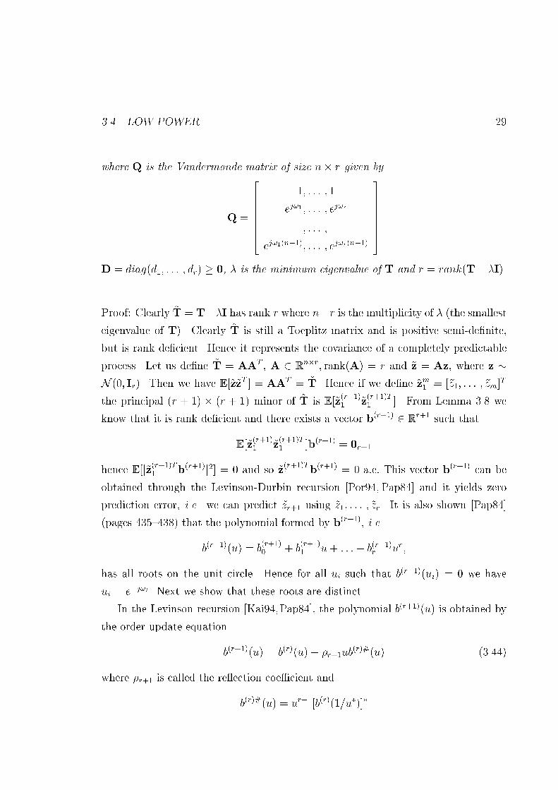
3.4. LOW POWER 29where Q is the Vandermonde matrix of size n� r given byQ = 2666664 1; : : : ; 1ej!1; : : : ; ej!r...; : : : ; ...ej!1(n�1); : : : ; ej!r(n�1)3777775D = diag(d1; : : : ; dr) � 0, � is the minimum eigenvalue of T and r = rank(T� �I).Proof: Clearly ~T = T��I has rank r where n�r is the multiplicity of � (the smallesteigenvalue of T). Clearly ~T is still a Toeplitz matrix and is positive semi-de�nite,but is rank de�cient. Hence it represents the covariance of a completely predictableprocess. Let us de�ne ~T = AAT , A 2 Rn�r; rank(A) = r and ~z = Az, where z �N (0; Ir). Then we have E [~z~zT ] = AAT = ~T. Hence if we de�ne ~zm1 = [~z1; : : : ; ~zm]Tthe principal (r + 1) � (r + 1) minor of ~T is E [~z(r+1)1 ~z(r+1)T1 ]. From Lemma 3.8 weknow that it is rank de�cient and there exists a vector b(r+1) 2 R r+1 such thatE [~z(r+1)1 ~z(r+1)T1 ]b(r+1) = 0r+1hence E [j~z(r+1)T1 b(r+1)j2] = 0 and so ~z(r+1)T1 b(r+1) = 0 a:e: This vector b(r+1) can beobtained through the Levinson-Durbin recursion [Por94, Pap84] and it yields zeroprediction error, i.e. we can predict ~zr+1 using ~z1; : : : ; ~zr. It is also shown [Pap84](pages 435{438) that the polynomial formed by b(r+1), i.e.b(r+1)(u) = b(r+1)0 + b(r+1)1 u+ : : :+ b(r+1)r ur;has all roots on the unit circle. Hence for all ui such that b(r+1)(ui) = 0 we haveui = e�j!i. Next we show that these roots are distinct.In the Levinson recursion [Kai94,Pap84], the polynomial b(r+1)(u) is obtained bythe order update equationb(r+1)(u) = b(r)(u)� �r+1ub(r)#(u) (3.44)where �r+1 is called the re ection coe�cient andb(r)#(u) = ur�1[b(r)(1=u�)]�

30 CHAPTER 3. WORST ADDITIVE NOISEand b(r)(u) is the error polynomial associated with the r � r principal minor of ~T.From lemma 3.8 we know that the r� r principal minor is positive de�nite and henceall the roots of b(r)(u) lie strictly within the unit circle. Hence we can represent b(r)(u)in terms of its roots �1; : : : ; �r�1 (where j�ij < 1) asb(r)(u) = C r�1Yi=1(u� �i): (3.45)We can also write the backward error prediction polynomial asb(r)#(u) = C� r�1Yi=1(1� ��i u): (3.46)Let u0 be any root of b(r+1)(u) and as we know that ju0j = 1 for all roots [Pap84], wecan write b(r)(u0) 6= 0 6= b(r)#(u0): (3.47)As u0 is a root of b(r+1)(u), using (3.44) we can writeb(r+1)(u0) = 0 = b(r)(u0)� �r+1ub(r)#(u0) (3.48)Using (3.44) we can writeddub(r+1)(u) = ddub(r)(u)� �r+1b(r)#(u)� �r+1u ddub(r)#(u): (3.49)If u0 is a multiple root of b(r+1)(u), then clearly it is also a root of ddub(r+1)(u). If u0is a multiple root, using (3.49) we can writeddub(r+1)(u)ju=u0 = 0 (3.50)= b(r)(u0) r�1Xi=1 1u0 � �i��r+1b(r)#(u0)� �r+1u0b(r)#(u0) r�1Xi=1 ���i1� ��i u0 ;

3.4. LOW POWER 31where we have used (3.45) and (3.46) to express ddub(r)(u) and ddub(r)#(u). Now using(3.48) we can rewrite (3.50) as,0 = ��r+1b(r)#(u0)[1 + u0 r�1Xi=1 ( ��i1� ��i u0 + 1u0 � �i )] (3.51)(a)= ��r+1b(r)#(u0)[1 + u0 r�1Xi=1 1� j�ij2ju0 � �ij2 ]where (a) follows due to the fact that 1u0 = u�0, as ju0j = 1. Note that from (3.47)b(r)#(u0) 6= 0 and as j�1j < 1; 8i, this means that 1 � j�ij2 > 0; 8i. Hence the righthand side of (3.51) cannot be zero. Therefore u0 cannot be a root of ddub(r+1)(u) andhence cannot be a multiple root of b(r+1)(u). Therefore all the roots of b(r+1)(u) aredistinct.This shows that the matrixQ = 2666664 1; : : : ; 1ej!1; : : : ; ej!r...; : : : ; ...ej!1(n�1); : : : ; ej!r(n�1)3777775where e�j!i = ui are the roots of b(r+1)(u) has full rank r. As e�j!i are the roots ofb(r+1)(u) we have[1; e�j!i; : : : ; e�j!i]2664 0lb(r+1)0n�(r+1)�l 3775 = 0 for i = 1; : : : ; r; l = 0; : : : ; n� (r + 1):From Lemma 3.8 we know that [0Tl ;b(r+1)T ; 0Tn�(r+1)�l]T ; l = 0; : : : ; n� (r+1) spansthe null space of ~T. Hence as Q� has rank r and Q�f = 0 for f in the null space of~T, Q has the same range space as ~T. Therefore if [r0; : : : ; rn�1]T is the �rst columnof ~T, the equation2666664 1; : : : ; 1ej!1; : : : ; ej!r...; : : : ; ...ej!1(n�1); : : : ; ej!r(n�1)
37777752664 d1...dr 3775 = 2664 r0...rn�1 3775 (3.52)

32 CHAPTER 3. WORST ADDITIVE NOISEhas a solution. Moreover, by construction using (3.52) and the fact that ~T is Toeplitzwe can write ~T = QDQ�where D = diag(d1; : : : ; dr) � 0 since ~T � 0. Hence we have the construction givenin (3.43). �Now we are ready to tackle the main completion problem.Theorem 3.4 The completion problem de�ned bymaxKz2Kz �min(Kz)as de�ned in (3.38) is solved by the n� n matrixKz = QDQ� + �I (3.53)where Q = 2666664 1; : : : ; 1ej!1; : : : ; ej!p...; : : : ; ...ej!1(n�1); : : : ; ej!p(n�1)3777775and D = diag(d1; : : : ; dp) � 0. Such a covariance arises from the following process:Zk = pXi=1 Viej!ik + �Wkwhere fVig; fWkg are independent normal random variables with Vi � N (0; di) andWk � N (0; 1)Proof: Consider T, the (p+1)� (p+1) leading minor of the n� n matrix Kz. Let �be the minimum eigenvalue of T. First we show that the minimum eigenvalue of any

3.4. LOW POWER 33n� n matrix Kz 2 Kz is less than or equal to �, for any n � p+ 1. Consider � 2 Rnand 2 R p+1, by the de�nition of minimum eigenvalue of Kz we have,�min(Kz) = minjj�jj2=1 �TKz� (3.54)(a)� min�=[ T ;0Tn�(p+1)]T ;jj jj2=1 �TKz�= minjj jj2=1 TT = �where (a) is due to the fact that we are minimizing over a smaller set. Hence anycompletion Kz 2 Kz has eigenvalue less than or equal to �. According to the bandedconstraint given in (3.29), T is Toeplitz positive semi-de�nite and completely speci-�ed. Hence using Theorem 3.3 we can writeT = QDQ� + �I (3.55)where � is the minimum eigenvalue ofT andQ is the (p+1)�(p+1�L) Vandermondematrix speci�ed in Theorem 3.3.Now consider the extensionKz = Q(n)DQ(n)� + �In; (3.56)where Q(n) is the Vandermonde matrix which is the n� (n�L) extension of Q givenby Q(n) = 2666664 1; : : : ; 1ej!1; : : : ; ej!p+1�L...; : : : ; ...ej!1(n�1); : : : ; ej!p+1�L(n�1)3777775 :By construction Kz is Toeplitz and due to (3.55) it satis�es the banded constraint Kz.Hence Kz 2 Kz and �min(Kz) = � by construction in (3.56). Therefore from (3.54)we see that this completion maximizes the minimum eigenvalue of any completion inKz. This proves the result and the construction given in the theorem is easily foundfrom (3.56). �Hence for very low signal power, the worst noise (in terms of mutual information)for the banded covariance constraint behaves like sinusoids in noise.

34 CHAPTER 3. WORST ADDITIVE NOISE3.5 Decoding schemeIt is di�cult for the receiver to form a maximum likelihood detection scheme for allnoise distributions. Therefore we propose to use a simpler detection scheme basedon a Gaussian metric and the second-order moments. However, as this is not theoptimal metric, it falls into the category of mismatched decoding [Lap95]. Thereforeit is not obvious that the rate 12 log jKx+KzjjKzj is achievable using such a mismatcheddecoding scheme. In this subsection we show that this rate is achievable using arandom Gaussian codebook and a Gaussian metric under some conditions on the noiseprocess. In [Lap95, Lap96], it was shown that 12 log(1 + P=N0) is achievable using aGaussian codebook and a minimum Euclidean distance decoding metric. This resultwas extended to the vector single user channel where the transmitter had access tothe noise covariance matrix and hence can form parallel channels [Lap95,Lap96]. Inour case we do not assume that the transmitter has access to the noise covarianceand show that if the receiver has access to Kz then rate 12 log jKx+KzjjKzj is achievable.The coding game is played as follows. The transmitter is allowed to choose arandom codebook, where the codebook and randomization are known to the receiver.The noise can choose any noise distribution with the given covariance constraints andthe receiver knows only the noise covariance and not its distribution. Now the receiverchooses a given decoding metric based on the knowledge of the noise covariance andthe random transmit codebook. In particular we use a Gaussian decoding rule for thereceiver. We �nd the highest rate for which the probability of error averaged over therandom codebooks goes to zero.Let us de�ne M(X(n);Y(n)) asM(X(n);Y(n)) = 12log jKx +KzjjKzj + 12Y(n)T (Kx +Kz)�1Y(n) (3.57)�12(Y(n) �X(n))TK�1z (Y(n) �X(n)):De�ne X(n) and Y(n) to be jointly �-typical if we have12n log jKx +KzjjKzj � 1nM(X(n);Y(n)) < �: (3.58)

3.5. DECODING SCHEME 35Our detection rule is that we declare X(n)(i) to be decoded if it is the only codewordwhich is jointly �-typical with the received Y(n). Note that the detection rule isequivalent to a Gaussian decoding metric with a threshold detection scheme whichdeclares an error if there is more than one codeword below the threshold. This canbe seen by rewriting (3.58) as,12n(Y(n) �X(n))TK�1z (Y(n) �X(n)) < 12nY(n)T (Kx +Kz)�1Y(n) + �: (3.59)The conditions that we impose on the noise process are:C1: limn!1Pr�j 1nz(n)TK�1z z(n) � E [ 1nz(n)TK�1z z(n)]j > �� = 0; 8� > 0.C2: limn!1Pr�j 1nz(n)T (Kx(1 + ) +Kz)�1z(n) � E [ 1nz(n)T (Kx(1 + ) +Kz)�1z(n)]j > �� =0; 8� > 0; > 0.We begin by stating two results which are proved in Appendix A. The secondresult requires the use of conditions C1 and C2.Lemma 3.9 If X(n) � N (0; Kx) and is independent of Y(n), then we have,E �exp�12Y(n)T (Kx +Kz)�1Y(n) � 12(Y(n) �X(n))TK�1z (Y(n) �X(n))�� (3.60)= exp(�12 log(jKx +Kzj=jKzj)):Lemma 3.10 If X(n) � N (0; Kx) and is independent of Z(n), and E [Z(n)Z(n)T ] =Kz > 0, and the noise satis�es C1 and C2, thenPr[ 12nZ(n)TK�1z Z(n) > 12n(Z(n) +X(n))T (Kx +Kz)�1(Z(n) +X(n)) + �] (3.61)� (1� �)exp(�n �28 ) + �:We de�ne P (n)e as the probability of error over a block of n samples. We will showbelow that for rates Rn below Cn = I(X�(n)G ;X�(n)G +Z�(n)G ) there exists codebooks forwhich the probability of error goes to zero asymptotically in n.Theorem 3.5 If the �-typical decoding scheme de�ned in (3.58) is used, � > 0, thenthere exists a sequence of (2n(Cn��); n) codes with P (n)e ! 0 as n ! 1, where Cn =

36 CHAPTER 3. WORST ADDITIVE NOISEI(X�(n)G ;X�(n)G +Z�(n)G ), and it is assumed that X(n) is chosen from a random codebookwhich is populated with independent codewords chosen from a Gaussian distributionwith covariance Kx, and the noise satis�es C1 and C2.Proof: Let X(n)(i); i = 1; : : : ; 2nRn be independent codewords chosen from a Gaussiandistribution with covarianceK�x. Let us de�ne the event Ei = fX(n)(i);Y(n) are jointly�-typical g, where typicality is de�ned in (3.58). As the index of the codewordsis assumed to be chosen from a uniform distribution we can assume w.l.o.g. thatX(n)(W );W = 1, was the transmitted codeword. Hence we can write the probabilityof error P [EjW = 1] using the union bound asP [EjW = 1] � Pr[Ec1] + 2nRnXi=2 Pr[Ei]: (3.62)We can write Pr[Ei] for i 6= 1 asPr[Ei] = Pr �1nM(X(n)(i);Y(n)) > 12n log jKx +KzjjKzj � �� (3.63)(a)� E [eM(X(n)(i);Y(n))�n�](b)= e 12 log( jKx+Kz jjKz j �n�)E �exp(12Y(n)T (Kx +Kz)�1Y(n)�12(Y(n) �X(n))TK�1z (Y(n) �X(n)))�(c)= e�n�(d)= e�n(Cn��)where (a) follows from the Cherno� bound, using � = Cn� � and Cn = 12n log jKx+KzjjKzj ;(b) follows by expanding M(X(n)(i);Y(n)); (c) uses Lemma 3.9, and (d) uses � =Cn � �. Therefore using (3.62) and (3.63) we have,P [EjW = 1] � Pr[Ec1] + e�n(Cn�Rn��) (3.64)(a)� (1� �)exp(�n�28 ) + �+ e�n(Cn�Rn��)where (a) follows from Lemma 3.10. Therefore, if Rn � Cn� � then limn!1 P [EjW =1] = 0. Hence we have the desired result using a random coding argument. �
3.6. SUMMARY 37This result needs to be interpreted with caution, as it is proved that the averageerror probability, averaged over random transmit codebooks, goes to zero and notshown for a deterministic coding scheme. Given this caveat, we have shown thatdespite having a mismatched decoder (which is matched to the Gaussian metric giventhe noise covariance matrix), we can transmit information reliably at rate Rn usinga random codebook populated by independent Gaussian codewords.3.6 SummaryIn this chapter we have studied the problem of communication over a class of additivecovariance constrained noise processes. The existence of Gaussian saddlepoints in themutual information game (under spectral constraints on signal and noise) imply therobustness of Gaussian codebooks. The problem of robust signal design reduces to�nding the worst noise processes with covariance constraints. We show that for highsignal power, the worst noise with a banded covariance constraint is the maximumentropy noise. However, the maximum entropy noise is not the worst noise for lowsignal powers. Hence robust signal design depends on the noise constraints as well asthe available transmit signal power.

Chapter 4Spatial diversity fading channelsIn this chapter we examine the achievable performance for multiple antenna diversity(or spatial diversity) fading channels. In particular we focus on communication struc-tures which have both transmitter and receiver antenna diversity. These structureshave received considerable recent attention as they could conceivably provide veryhigh data rate communication.Achievable performance over fading channels has been a subject of interest forseveral decades, see [Pro95,OSW94,KS94, SW97,CTVTB97] and references therein.In the past, the focus was on receive spatial diversity. Spatial transmit diversity hasbeen examined recently in [WT97,NTW96]. Recent results in [Fos96,TSC98,Tse97,Tel95,RC96] suggest signi�cant advantages in using both transmit and receive spatialdiversities.There has been a large body of work devoted to data transmission over time-invariant frequency selective channels [Pro95]. Transmit and receive diversity overtime-invariant frequency selective (ISI) channels have been examined in [YR94,BS92,RC96] and references therein. Reliable transmission over time-varying ISI channelshas been studied in [Gol94,Med95,OSW94]. In [Gol94,Med95] it is assumed that boththe transmitter and the receiver know the channel realization. In [OSW94] only thereceiver is assumed to know the channel state but a quasi-static channel is assumed.The quasi-static assumption is that the channel is assumed to be time-invariant overthe transmission block. This assumption makes the results in [OSW94] suitable for38

39slowly time-varying channels. In this chapter we examine the impact of time-variationon reliable transmission. We examine performance with transmit and receive diversityboth for the at fading case and when we have a time-varying ISI channels.In this chapter we study di�erent communication structures in terms of mutualinformation and cut-o� rate. Mutual information represents the achievable rate forreliable communications and is a good measure for performance.In Section 4.2 we explore the at fading diversity channel. It was reported recentlyin [Fos96] that the mutual information grows linearly with the number of spatial di-versity elements (asymptotically as the number of antennas becomes very large). Weprovide and alternative approach to this result by using an asymptotic decouplingargument. In this we show that by using a \linear detector", i.e. a matched �l-ter followed by decoupled (across diversity channels) detection, we still get a lineargrowth in mutual information with the number of spatial diversity elements. There-fore, even with a suboptimal (not maximum likelihood) detection scheme which hasmuch lower complexity, we still obtain similar trends as the optimal decoding schemeused in [Fos96]. However, linear growth is obtained under the assumption that thechannel gain becomes unbounded resulting in unbounded achievable rates. The re-sult in [Fos96] also critically depends on this assumption. Consequently we examinea channel with unit average gain and show that mutual information grows linearlywith signal-to-noise ratio (SNR) as the number of diversity elements becomes large.Additionally we show at high SNR, the mutual information is linear in the number ofspatial diversity elements (on both the transmitter and the receiver). This high SNRbehaviour has also been observed in the context of time-invariant channels [RC96].The cut-o� rate is considered an important parameter in practical code designand is discussed in [Pro95]. We derive the cut-o� rate of the spatial diversity channelwhen the transmitter has partial channel knowledge, i.e., it knows only the spatialcorrelation behavior of the fading channel. The cut-o� rate can be used to evaluatethe gains in using coding over multiple antennas, e.g. space-time codes [TSC98].Next, we study the mutual information for time-varying ISI channels and considerboth the slowly time-varying (i.e., block time-invariant) and the fast time-varyingchannel. We �rst derive the achievable rate for multiple transmitter and receiver

40 CHAPTER 4. SPATIAL DIVERSITY FADING CHANNELSdiversity in slowly fading channels. Multicarrier transmission is an e�cient trans-mission structure for time-invariant ISI channels. Recently multicarrier transmissionover diversity channels has been proposed in [CDS96]. We derive the achievable ratefor OFDM over time-varying ISI channels. Using this result we examine the impactof transmit diversity and receive diversity on OFDM transmission in time-varyingchannels. As expected we show that the performance depends on the amount ofinter-carrier interference (ICI). If the channel is almost time-invariant over the trans-mitted block, neglecting the ICI results in only a small loss in performance. In OFDMthere is a cyclic pre�x (or a guard interval) equal to the length of the channel withevery transmitted block. This results in an overhead that becomes a smaller fractionof the total rate when the block size increases. For fast time-varying channels, ifwe use longer packets the loss would be greater (if we ignore ICI) and hence thereis an inherent trade-o� of performance with transmission overhead. Moreover, if wedecode the signals jointly over all carriers (i.e. equalize the channel), then we get per-formance enhancement at the cost of higher complexity. Therefore, these trade-o�sare important in packet size design as well as transceiver design. These results helpus understand the role of equalization in time-varying ISI channels.A brief outline of this chapter is as follows. In Section 4.2 we derive the achievableperformance over at fading diversity channels. Section 4.3 focuses on multicarriertransmission over fading ISI channels. In Section 4.4 we provide numerical examplesfor the results developed. Some of the detailed proofs are given in the appendices.4.1 Data modelWe use the discrete time model given in Chapter 2 equation (2.5)y(k) = L�1Xl=0 H(k; l)x(k � l) + z(k); (4.1)where H(k; l) 2 CM�N is the lth tap of the matrix response with x(k) 2 CN istransmitted signal, y(k) 2 CM is the received signal and z(k) 2 CM is the complexadditive temporally white Gaussian noise with z(k) � CN (0;Rz), i.e. a complex
4.1. DATA MODEL 41Gaussian vector with mean 0 and covariance Rz. Also as in Chapter 2, L is thenumber of taps in the ISI channel, M is the number of receive antennas and N isthe number of transmit antennas. Throughout this chapter we impose an averagepower constraint on the input, i.e. E [jjx(k)jj2] � P . Structure of fH(k; l)g couldbe constructed by assigning a special structure to H(c)(t; �) (for example a discretemultipath channel). We assume a statistical description of the channel in an attemptto balance practical utility and analytical tractability. In both the at fading and theISI cases, we use the the assumption of ideal interleaving. This is not critical, thoughit simpli�es achievable rate arguments. The mutual information expressions derivedalso hold when the channel is an ergodic process as shown in [OSW94,SW97].4.1.1 Flat fading channelIn this case L = 1 and the single tap H(k; 0) is denoted for brevity by H(k). We canrewrite (4.1) as y(k) = H(k)x(k) + z(k): (4.2)We assume that the elements of H(k) are i.i.d. complex Gaussian, i.e. H(k) =[h1(k); : : : ;hN(k)] has Hi;j(k) � CN (0; 1) i.i.d. elements. This could be justi�edwhen the antennas are separated far enough apart so that the fading on each of thelinks are independent. Note that the there is a linear \array" gain associated withthis model in that the average channel gain grows linearly with the number of receiveantennas (E jjhi(k)jj2 = M). This gain captures the e�ect of gathering more energywhen we add more receive antennas. We also consider a model when we have capturedall the energy transmitted and we do not have an average gain from the channel. Inthis case we consider a model where the L2 norm of each column of H(k) is unity, i.e.E jjhi(k)jj = 1 and Hi;j(k) � CN (0; 1=M). This represents a passive channel havingno average gain. We also assume for the at fading channel considered in Section 4.2that we have ideal interleaving, i.e. H(k) is temporally i.i.d.

42 CHAPTER 4. SPATIAL DIVERSITY FADING CHANNELS4.1.2 The ISI channelIn the problem considered in Section 4.3, we have a time-varying ISI channel describedin (4.1). For convenience we use the Wide-Sense Stationary Uncorrelated Scattering(WSSUS) model commonly used in describing scalar fading channels [Jak74]. In thismodel, the channel fH(k; l)g is modeled as a Gaussian stochastic process with theproperty that E [H(k;n)HH(k;m)] = E [H(k;n)HH(k;m)]�[n � m]. In this case wecannot assume symbol-by-symbol ideal interleaving because of ISI. However, when wetransmit using OFDM packets we can assume that we have ideal packet interleaving.We invoke this model in Section 4.3 to gain insight into transmission over fadingchannels.4.2 Achievable performance in at fading channelsIn this section we examine the advantages of using spatial diversity in at-fadingenvironments. In subsection 4.2.1 we review the capacity of this channel. In subsec-tion 4.2.2 we show that the linear asymptotic growth of the mutual information withnumber of antennas occurs when we use a decoupled detection scheme. A passivechannel where the average channel gain is normalized, is examined in Section 4.2.3.In this case the mutual information grows linearly with SNR asymptotically with thenumber of antennas. In subsection 4.2.4 we show that the linear gain also occurswhen the SNR becomes very large. Finally in subsection 4.2.5 we examine the cut-o�rate and using this we examine the coding gains for some �nite PSK constellationsin Section 4.4.4.2.1 CapacityIn this section we assume the at fading channel model described in Section 4.1.1.The receiver is assumed to have perfect channel state information (CSI) and thetransmitter only knows the statistics of the channel. We also assume that we haveideal interleaving so that the fading process is memoryless. Using these assumptions

4.2. ACHIEVABLE PERFORMANCE IN FLAT FADING CHANNELS 43the mutual information for a block of n time samples can be written as1nI(x(n);y(n);H(n)) = 1n hI(x(n);H(n)) + I(x(n);y(n)jH(n))i (4.3)(a)= 1nE H[I(x(n);y(n)jH(n) = fH(n)g)](b)= E H[log( jRz +HRxHH jjRzj )];where (a) follows from the fact that the input fx(k)g is independent of the fadingprocess (as the transmitter does not have CSI) and (b) follows from the memorylessproperty of the vector Gaussian channel obtained by conditioning on H(k). We usei.i.d. Gaussian input fx(k)g with Rx = E [x(k)x(k)H ], as this maximizes the mutualinformation conditioned on H. In general it is di�cult to evaluate (4.3) except forsome special cases. If we assume Rz = �2I, and if we have independent diversity, i.e.if H(k) consists of iid Gaussian elements it can be shown [Tel95] thatC = EH[log(jI + PN�2HHH j)] (4.4)is the capacity of the fading matrix channel, where Rx = PN I. This expression canbe evaluated using properties of Wishart matrices and represented in a numericallycomputable form [Tel95,Mui82,Ede89,Tse97].4.2.2 Decoupled detectionTo achieve the capacity given in (4.4) we require joint optimal (maximum-likelihood)decoding of all the receiver elements. In this section we explore the performance of asub-optimal \linear decoding" scheme which is similar in avor to the matched �lterreceiver studied in multi-user detection [Ver98]. Due to the decoupling propertiesof the channel, we show that this detector still retains the linear growth rate of theoptimal decoding scheme. However, we do pay a price in terms of growth rate withSNR.In the following we will assume that H(k) has iid elements, (Hi;j(k) � CN (0; 1))and Rz = �2I and N = M unless otherwise stated. Note that from the data modelgiven in (4.2), the maximum likelihood decoding rule forRz = �2I is minfx(k)gXk jjy(k)�

44 CHAPTER 4. SPATIAL DIVERSITY FADING CHANNELSH(k)x(k)jj2. Hence a su�cient statistic would be ~y(k) = HH(k)y(k), and thus,~y(k) = HH(k)H(k)x(k) +HH(k)z(k) (4.5)We have I(x; ~y;H) = I(x;y;H) because there is a one-to-one mapping between ~yand y (due to H(k) being full rank a.s.). hence In [Fos96] it has been stated thatthe mutual information grows linearly with M as M ! 1, i.e. limM!1 I(x;y;H)M =constant. A proof outline is provided in [Fos96] for this using a layered architecturewherein the problem is treated akin to a multiple access channel and decoding isdone using an onion peeling scheme with orthogonal projection. In the followingwe provide an alternative approach which demonstrates the linear growth and alsoshows the importance of \interference cancellation". As we have Hi;j(k) � CN (0; 1),and the elements of H are i.i.d., due to the strong law of large numbers (SLLN)limN!1 hHi (k)hj(k)=N = �i�j a:s:, where �k is the Kronecker delta function.As the channels asymptotically decouple we investigate the rate achievable ifwe ignore the cross-coupling of the channels when decoding. If we denote ~z(k) =HH(k)z(k), we can write the ith component of ~y(k) in (4.5) as~yi(k) = jjhi(k)jj2xi(k) +Xj 6=i hHi (k)hj(k)xj(k) + ~zi(k); i = 1; : : : ;M: (4.6)By ignoring the cross-coupling between the channels we decode xi as minxiPk j~yi(k)�jjhi(k)jj2xi(k)j2 and hence we include the \interference" from fxjgj 6=i as part of thenoise. This is identical to the matched �lter receiver studied in multiuser detectionschemes [Ver98]. Using almost identical arguments as in (4.3) we can show that themutual information I(xi; ~yi;H) can be written asI(xi; ~yi;H) = E "log 1 + (jjhijj2)2P=Mjjhijj2�2 + (Pj 6=i jhHi hjj2)P=M!# : (4.7)Hence the total rate achievable (RI) when we ignore the cross-coupling is given byRI = E " MXi=1 log 1 + (jjhijj2)2P=Mjjhijj2�2 + (Pj 6=i jhHi hjj2)P=M!# ; (4.8)(a)= ME "log 1 + (jjhijj2)2P=Mjjhijj2�2 + (Pj 6=i jhHi hjj2)P=M!#

4.2. ACHIEVABLE PERFORMANCE IN FLAT FADING CHANNELS 45where (a) follows due to the i.i.d. assumption on the fading channels. By the SLLN,limM!1 jjhi(k)jj2=M = 1 a.s. We show in Appendix B.1 that limM!1Xi 6=j jhHi (k)hj(k)=M j2 =1 a.s. Hence using these two facts we havelimM!1 log 1 + (jjhijj2)2P=Mjjhijj2�2 + (Pj 6=i jhHi hjj2)P=M! = log(1 + P=�21 + P=�2 ) a:s: (4.9)as log(�) is a continuous function. It is shown in Appendix B.1 that we can exchangelimits and expectations to getlimM!1RI=M = limM!1 E "log 1 + (jjhijj2)2P=Mjjhijj2�2 + (Pj 6=i jhHi hjj2)P=M!# (4.10)= E " limM!1 log 1 + (jjhijj2)2P=Mjjhijj2�2 + (Pj 6=i jhHi hjj2)P=M!# :Hence we have proved the following result.Proposition 4.1 IfHi;j(k) � CN (0; 1), then limM!1 1M I(y;H;x) � limM!1RI=M =log(1 + P=�21+P=�2 ). �Hence, using a decoupled detection scheme which has signi�cantly lower com-plexity than the optimal scheme, we still obtain asymptotically linear growth ratein mutual information with number of antenna elements. The analysis also demon-strates the importance of joint decoding. We see that if the other transmit channelsare regarded as noise, even though the channels asymptotically decouple, the contri-bution from the \interference" limits performance. Hence the improvement in ratewith SNR requires joint detection of all the transmit codebooks.4.2.3 Passive channelIn the above analysis channel gain goes to in�nity and hence so does the rate whichgrows asymptotically linearly in M . Next, we investigate the behavior in the casewhere the channel gain is unity, i.e., the L2 norm of each of the columns of H(k) is

46 CHAPTER 4. SPATIAL DIVERSITY FADING CHANNELSunity (Hi;j(k) � CN (0; 1=M)). A general upper bound on the mutual informationin this case can be obtained through Jensen's inequality.E [log jI+ PN�2HHH j] � log jI(1 + PN�2 )j (4.11)where we have used Jensen's inequality on the concave function log det[�] and the factthat E [HHH ] = I. Hence letting N !1 in (4.11) we get the relationship,limM;N!1 E [log jI+ PN�2HHH j] � P�2 (4.12)In the sequel we explore the tightness of this upper bound. In (4.4) if we letM !1,then we would get limM!1 I(x;y;H) = N log(1 + PN�2 ). Since limM!1HHH =IN a:s:. Now if we let N !1 we getlimN!1 limM!1 I(x;y;H) = P�2 : (4.13)This argument demonstrates that the channel behaves like N decoupled straight wirechannels as M ! 1 and hence resembles the in�nite bandwidth Gaussian channelresult [CT91]. This is also true if we let N ! 1 �rst and then M ! 1. However,when we haveM = N and then let them go to in�nity the above argument is incorrect,but a similar result can be proved with a more technical argument shown below.In [Fos96] a lower bound on jI + PN�2HHH j is developed and an informal proofoutline was provided. Here we provide a more rigorous proof of this inequality.Proposition 4.2 If x � CN (0; �IM) and A = [a1; : : : ; aK ] 2 CM�K is a randommatrix independent of x and aHi aj = �i�j, then AHx � CN (0; �IK).Proof: Let z = AHx, then we can write its conditional density function as,fzjA(zjA) = exp(�zHz=�)(�)K�K (4.14)as x is independent of A and AHA = I. Averaging over the distribution of A, as(4.14) does not depend on A we obtain the desired result. �

4.2. ACHIEVABLE PERFORMANCE IN FLAT FADING CHANNELS 47This proposition can be used to formalize (4.18) using the onion-peeling withprojection idea in [Fos96]. We can write (4.2) as,y(1)(k) = y(k) = h1(k)x1(k) + : : :+ hN(k)xN (k) + z(k) (4.15)Thus as in [Fos96] in the lth stage we have already decoded x1; : : : ;xl�1 and we havesubtracted its contributions from y(k) to obtain y(l) = PNi=l hi(k)xi(k) + z(k). Todecode xl(k) we project y(l) onto the space orthogonal to spanfhl+1(k); : : : ;hN(k)g.The orthonormal basis for this space is a random basis which is a deterministicfunction of the random vectors fhl+1(k); : : : ;hN(k)g and hence is independent ofhl(k). Hence if we denote the projection matrix by Al(k) and we denote ~y(l)(k) =AHl (k)y(l)(k) as the projected vector we obtain,~y(l)(k) = AHl (k)hl(k)xl(k) +AHl (k)z(k) (4.16)as AHl (k)hi(k) = 0; i = l + 1; : : : ; N . Now using Proposition 4.2 we have thatAHl (k)hl(k) � CN (0; Il=N) and AHl (k)z(k) � CN (0; �2Il). Thus following argu-ments almost identical to (4.3) we have,R(l) = I(~y(l);H;xl) = E [log(1 + P�2N2�22l)] (4.17)where �22l is a chi-squared random variable with 2l degrees of freedom and E [�22l] = l.Thus we obtain the overall rate as R = PNl=1R(l) which is achievable and a lowerbound to I(x;y;H) and hence we obtain the following,I(x;y;H) � E [ MXi=1 log(1 + P�2M2�22i)] (4.18)where �22i is a chi-squared random variable with 2i degrees of freedom and E [�22i] = i.If we denote �22i = Pij=1 jUjj2 where Uj � CN (0; 1) i:i:d: then it is shown inAppendix C thatlimM!1 MXi=1 log(1 + P�2M2�22i) = limM!1 MXi=1 P�2M2 iXj=1 jUjj2 = P2�2 a:s: (4.19)Using this and by exchanging limits and expectation in (4.18) (as explained in Ap-pendix C) we have the following result.

48 CHAPTER 4. SPATIAL DIVERSITY FADING CHANNELSProposition 4.3 If Hi;j(k) � CN (0; 1=M), then P�2 � limM!1I(y;H;x) � P2�2 . �Here we get a factor of half over the result in (4.13) because of the inequality in(4.18).4.2.4 Finite diversityIn the previous sections we have let the number of diversity elements become verylarge. In this section we investigate the case where the SNR becomes very large,but the number of diversity elements is �nite. Let RM;N be the rate achievable forM receiver and N transmitter antennas. In the following proposition we considerthe case where, Hi;j(k) � CN (0; 1), and its extension to the case where Hi;j(k) �CN (0; 1=M) is straightforward.Proposition 4.4 liminfP=�2!1RM;MRM;1 �MProof:RM;1 = E [log(1 + jjhjj2P=�2)] (a)� log(1 + E [jjhjj2]P=�2) = log(1 +MP=�2) (4.20)where (a) is due to Jensen's inequality. Now we lower bound RM;M asRM;M = E [log(jI+HHH PM�2 j)] (4.21)= E [ MXi=1 log(1 + �i(HHH) PM�2 )](a)� E [M log(1 + �min(HHH) PM�2 )](b)� M log(1 + � PM�2 )Pr(�min(HHH) > �);where �i(�) is the eigenvalue and (b) is true for all � > 0. Now to investigate theP=�2 ! 1 we let P=�2 = exp(1=�). When we let � ! 0, P=�2 ! 1. Now, bycombining (4.20), (4.21) and using P=�2 = exp(1=�) we obtainRM;MRM;1 �M log(1 + �exp(1=�)=M)log(1 +Mexp(1=�)) Pr(�min(HHH) > �) (4.22)

4.2. ACHIEVABLE PERFORMANCE IN FLAT FADING CHANNELS 49By letting � ! 0, we let P=�2 ! 1. Now lim�!0 Pr(�min(HHH) > �) = 1 and wecan show by using L'Hospital's rule that lim�!0 log(1+�exp(1=�)=M)log(1+Mexp(1=�)) = 1. By substitutingthese results into (4.22) we get the desired result. �In the above result, if N 6=M , by a simple extension of the above argument it canbe shown that liminfRM;NRM;1 � min(M;N). Thus the gain is dictated by the number ofparallel channels created by the matrix channel. The basic intuition behind this resultis that we have min(M;N) cross-coupled channels when there areM transmitters andN receivers. Hence when N = 1 (or M = 1) we have e�ectively only one channel andthe gain in using multiple antennas at both the transmitter and the receiver end is increating more cross-coupled channels. These results indicate the advantages of usingmultiple spatial diversity elements at both the transmitter and the receiver.4.2.5 Cut-o� rateCut-o� rate is considered an important measure of system performance [Mas74]. Wetherefore compute the cut-o� rate for the diversity fading channel. This is also moti-vated by two other reasons, �rst the cut-o� rate allows us to compare the performanceof inputs modulated by �nite constellations. Secondly we can observe the e�ects ofcorrelation in the channel and noise.The pairwise error probability between two sequences fx(k)g and fx(k)g can beupper bounded by the the Cherno� bound asPr(fx(k)g ! fx(k)gjH) �Yk exp(� ( � 1)hH(k)EH(k)R�1z E(k)h(k)) (4.23)where is the Cherno� parameter, E(k) = eH(k) IM , h(k) = vec(H(k)), e(k) =x(k)� x(k), vec(�) stacks the matrix into a vector column-by-column [Bre78] and indicates the Kronecker product. Hence using the fact that h(k) � CN (0;Rh) iid,and optimizing over we obtain,Pr(fx(k)g ! fx(k)g) �Yk 1jI+ 14(e(k)eH(k)R�1z )Rhj (4.24)Using the de�nition of cut-o� rate R0 = � 1n log E [Pr(fx(k)g ! fx(k)g)] we obtain,R0 = � log E e[ 1jI+ 14(eeH R�1z )Rhj ] (4.25)

50 CHAPTER 4. SPATIAL DIVERSITY FADING CHANNELSThis result is used in the numerical examples presented in Section 4.4. It is usedboth in comparison between achievable rates for Gaussian codebooks and for �niteconstellation modulation schemes (e.g. PSK constellations).4.3 Frequency selective fadingReliable transmission in frequency selective fading channels has been studied ex-tensively in literature, [Pro95, OSW94] and references therein. The most commonassumption in studying these schemes is that of slow time-variation (i.e. Bandwidth� Doppler spread). The rate of reliable information for the scalar channel has beenderived in [OSW94] in terms of the expected mutual information. We begin thissection with a simple extension of this result to the case of transmitter and receiverdiversity in Section 4.3.1. In Section 4.3.2 we focus on the impact of time-variationwithin a transmission block and mainly analyze performance of multicarrier trans-mission schemes in such a scenario. We specialize the results of Section 4.3.2 to theWSSUS model (see Section 4.1.2) in Section 4.3.3.4.3.1 Slowly time-varying channelsConsider the model speci�ed in Section 4.1 (2.5). If we use the average power con-straint given by E [jjx(k)jj2] � P , we can de�ne for a block of size n,Rn = 1nI(x(n);y(n);H(n)) (4.26)where x(n) = [x(0)T ; : : : ;x(n � 1)]T , y(n) = [y(0)T ; : : : ;y(n � 1)]T and H(n) =fH(k; l)gn�1k=0; l 2 [0; : : : ; L � 1]. In the ISI channel we assume that a guard inter-val of L samples exists between the transmission blocks. Note that this �xed intervaldoes not lower the transmission rate asymptotically in the block size n. In the abovewe have assumed that the guard interval x(�L); : : :x(�1) is a deterministic functionof x(n). By using arguments identical to (4.3) we can show that if the transmitter hasno knowledge of the channel realization then,Rn = 1nE [I(x(n);y(n)jH = H(n))]: (4.27)
4.3. FREQUENCY SELECTIVE FADING 51Conditioned on H(n) the channel (2.5) becomes an additive Gaussian channel. Theslowly time-varying channel assumption is that the channel is time-invariant over atransmission block, i.e. H(k; l) = H(r; l); 8r; k 2 [0; : : : ; n� 1]; 8l. Now, to evaluate(4.27) we can use the DFT-based approach for the achievable rate of discrete timeGaussian channels developed in [HM88]. Let us �rst assume that we have appendeda circular pre�x in the guard interval, i.e. x(�k) = x(n � k); k = 1; : : : ; L, which islike OFDM [Cio94]. This is called as the N-circular Gaussian channel in [HM88] andusing similar arguments we can show that the achievable rate ( ~Rn) for this channelis, ~Rn = 1nE [I(x(n); ~y(n)jH = H(n))] (4.28)(a)= 1nE [n�1Xp=0 log(j ~H(p)S(p) ~HH(p)=�2 + Ij)where we have de�ned the output of the circular channel as ~y(n), (a) is obtainedby using Gaussian inputs x(n) and de�ning ~H(p) = Pn�1l=0 H(0; l)�pl where =exp(�j2�=n); j = p�1. As in (4.3) the Gaussian input maximizes the mutual infor-mation and using the block time-invariance assumption we use a stationary Gaussiancodebook with correlation function Rx(l) = E [x(k)xH(k + l)]. We have also de�nedthe input power spectral density as S(p) = Pn�1l=0 Rx(l)�pl. We can easily showusing properties of Riemann integrals (see [HM88] for details of this argument) that,limn!1 1n [I(x(n);y(n)jH = H(n))] = limn!1 1nI(x(n); ~y(n)jH = H(n)) (4.29)= (2�)�1 Z log(jH(f)S(f)HH(f)=�2 + Ij)dfwhereH(f) and S(f) are the Fourier transforms of fH(0; l)g and fRx(l)g respectively.Hence we can show that,limn!1Rn = limn!1 ~Rn = (2�)�1E [Z log(jH(f)S(f)HH(f)=�2 + Ij)df ] (4.30)using arguments similar to those in Appendix C to exchange limits and expectations.Thus for slowly time-varying channels the achievable rate is well approximated by(4.30). In general maximizing (4.30) with respect to S(f) is a hard problem and

52 CHAPTER 4. SPATIAL DIVERSITY FADING CHANNELSfurther simplifying assumptions need to be made for solving this problem. How-ever, schemes using a at input spectrum in both time and \space" may be practi-cal [TSC98, CDS96] and therefore it is worthwhile to study them. In time-varyingchannels there is an inherent con ict between increasing the transmission block length(for coding arguments) and the block time-invariance assumption. This is a topic wewill explore in the next section.4.3.2 Impact of fast time-variationThe relation (4.27) holds even when we do not invoke the block time-invariance as-sumption. To gain an understanding of this problem, let us consider the scalar channelwith M = N = 1. Let us assume that the transmitter chooses an orthonormal basisfor transmission. For time-invariant channels it is known that asymptotically theFourier basis is optimal. For time-varying channels when the channel is unknown atthe transmitter, this remains an open problem. However, due to the low complexityof using the Fourier basis and the prevalence of practical schemes using it, this is aninteresting case to focus on. In time-invariant channels, the Fourier basis allows us toform parallel ISI-free channels and this scheme is illustrated in Figure 4.1. However,in time-varying channels, the Fourier basis is not in general an eigenbasis. This lossof orthogonality causes Inter-Carrier Interference (ICI). In this section we derive theinformation rates achievable in the presence of ICI.We can write the output of the DFT at the receiver for a time-block [�L; : : : ; n�1]as, Y (p) = G(p; p)X(p) +Xp6=q G(p; q)X(q) + Z(p) (4.31)for p = 0; : : : ; n � 1, where Y (p); X(p) and Z(p) are the DFTs of fy(k)g; fx(k)gand fz(k)g respectively. We have also de�ned G(p; q) as the (p; q)th element of G =Q �H(n)QH=n. Here Q is the DFT matrix de�ned as QH = [q0; : : :qn�1] and qs =[1; : : : ; exp(j2�s(n�1)=n)]T , and �H(n) is the equivalent channel matrix including the

4.3. FREQUENCY SELECTIVE FADING 53e�ects of the cyclic pre�x (used in OFDM) de�ned as2666666666664h(0; 0); 0; : : : ; 0; h(0;L� 1); : : : ; : : : ; h(0; 1)h(1; 1); h(1; 0); 0; : : : ; 0; h(1;L� 1); : : : ; h(1; 2)...h(L� 1;L� 1); : : : ; h(L� 1; 0); 0; : : : ; 0; : : : ; 0...0; : : : ; 0; : : : ; 0; h(n� 1;L� 1); : : : ; h(n� 1; 0)
3777777777775 : (4.32)We can easily evaluate G(m; s) as,G(m; s) = 1n n�1Xr=0 L�1Xl=0 h(r; l)ej2�r(s�m)=ne�j2�sl=n: (4.33)Note that the form of the model in (4.31) is applicable to more general cases thanusing OFDM. We can replace Q by any arbitrary matrix B and for a given structureof the guard interval (pre�x), we can �nd the speci�c structure of G (as in (4.33) forOFDM) for that case. We can rewrite (4.31) as,Y = GX+ Z (4.34)whereY = [Y (0); : : : ; Y (n�1)]T ,X = [X(0); : : : ; X(n�1)]T and Z = [z(0); : : : ; z(n�1)]T . Thus we can write Rn given in (4.27) as,Rn = E [log jI+GGHP=�2j] (4.35)where we have assumed independent Gaussian codebooks on each of the frequencybins. Note that the rate given in (4.35) is achievable if we assume ideal packetinterleaving (i.e. the matrix �H is identically distributed from packet to packet andis independent between packets). Here all the subcarriers need to be decoded jointly,which would imply that equalization (such as MLSE [For72]) in the frequency domainneeds to be employed. Therefore, a natural question that arises is the rate loss thatoccurs if we ignored the ICI while decoding, as is typically done in OFDM. Thequestion is similar to that posed in Proposition 4.1 for diversity channels and hencewe expect a similar answer. Using an argument almost identical to that used inobtaining (4.7), we can show that for an OFDM of packet size n, the rate achievable

54 CHAPTER 4. SPATIAL DIVERSITY FADING CHANNELSper transmitted sample is,ROFDM;n = 1nEG[n�1Xp=0 log(1 + jG(p; p)j2P�2 +Pq 6=p jG(p; q)j2P )]: (4.36)Thus we see that the rate loss directly depends upon the amount of ICI as we wouldintuitively expect. In the above we have assumed that we use a Gaussian inputcodebook and that the codebooks for each subcarrier is independent. The easiestcoding theorem proof for the above mutual information rate assumes independentfading on successive transmission blocks. Though this could be justi�ed by an idealpacket interleaving assumption, a more general proof can be based on ergodicityassumptions on the channel impulse response. Note that we have not made anyassumptions on the independence between G(p; p) and fG(p; q)g in this relationship.Also we need only the instantaneous SNR at the receiver to achieve this rate. Weknow from the results in at fading channels that spatial diversity reduces variabilityof the channel. The next question is whether having transmit diversity helps us inthis problem. For transmit diversity the expression in (4.36) can be easily modi�ed.We examine the case when the number of transmit antennas N is very large and wehave independent fading channels. This model is similar to the one used in 4.1.1. Inthis case when N !1 we have,R(N)OFDM;n = 1n n�1Xp=0 EG[log(1 + PPN�1d=0 jG(d)(p; p)j2=N�2 + PPq 6=pPN�1d=0 jG(d)(p; q)j2=N )] (4.37)N!1! 1n n�1Xp=0 log(1 + PE [jG(p; p)j2]�2 + PPq 6=p E [jG(p; q)j2] )where G(d) = Q �H(d)QH and �H(d) is the channel given in (4.32) for the dth diversityelement. We have assumed that independent Gaussian codebooks of power P=N areused at each of the transmit antennas and OFDM subcarriers. We get the above byusing strong law of large numbers (SLLN) and exchanging limits and expectations(easily justi�ed in a manner similar to Appendix B.1). An interesting phenomenonoccurs here due to the averaging e�ects of transmit diversity. If there were no ICI,such averaging would always increase the information rate by Jensen's inequality.
4.3. FREQUENCY SELECTIVE FADING 55However, as both the ICI and the signal are averaged it is not necessary that the rateincreases. This property is illustrated in the numerical example given in Section 4.4.A similar result has been observed in fading multiple access channels in the context ofbroadband vs narrowband transmission [SW97]. Thus transmit diversity would notalways help if the ICI is ignored. However, we do expect it to help if the amount ofICI is small (i.e. slowly varying channels).In the case when we have transmit and receive diversities we can modify (4.31) asY(p) = G(p; p)X(p) +Xq 6=pG(p; q)X(q) + Z(p) (4.38)where [G(p; q)]i;j = [QH(i;j)QH=n]p;q and H(i;j) is the equivalent channel matrix (asin (4.32)) for the time-varying ISI channel from the ith transmitter to the jth re-ceiver, fh(i;j)(k; l)g. Also the received vector for the pth frequency bin is Y(p) =[Y (1)(p); : : : ; Y (M)(p)]T , X(p) = [X(1)(p); : : : ; X(N)(p)]T is the transmitted vector forthe pth frequency bin and Z(p) = [Z(1)(p); : : : ; Z(M)(p)]T is the noise. Hence we caneasily write the achievable rate (if we use independent Gaussian codebooks on thedi�erent frequencies and the diversity elements) as,R(M�N)n = 1nE �log jI+ ~G ~GH PN�2 j� (4.39)(a)= 1nE �log jI+ ~H ~HH PN�2 j�where ~G is a block matrix consisting of M � N blocks of n � n matrices with the(i; j)th block given by QH(i;j)QH=n. Thus we can write ~G = ~Q1 ~H ~Q2=n, with ~Hhaving M �N blocks of the type H(i;j), and ~Q1 and ~Q2 are block diagonal matriceshaving M and N blocks respectively with Q as the block elements. Using the factthat ~Q1 and ~Q2 are unitary matrices we get (a) in (4.39). Though ~H ~HH is Wishartdistributed [Mui82], there does not seem to be a simple closed form solution to (4.39).To achieve the rate in (4.39), we need to do joint decoding of all the codebooks. Dueto the huge complexity, if there is signi�cant ICI we can decode using the \onion-peeling" principle by treating (4.38) as a matrix multiple access channel. The otheroption is to ignore the ICI and as in (4.36) we can write the rate achievable (if the

56 CHAPTER 4. SPATIAL DIVERSITY FADING CHANNELSICI is considered part of the noise) asR(M�N)OFDM;n = 1n n�1Xp=0 E log" jI+PqG(p; q)GH(p; q)P=N�2jjI+Pq 6=pG(p; q)GH(p; q)P=N�2j# : (4.40)Here we can envisage several techniques which are popular in spatio-temporal pro-cessing to get better performance for reasonable complexity. We can suppress the ICIusing the receive sensors and interference suppression techniques [WSG94,DNP98].Therefore, we expect that receive diversity will always help performance even whenwe ignore the ICI.4.3.3 The WSSUS channelWe specialize the results of Section 4.3.2 to the WSSUS model described in Section 4.1and focus on the scalar channel. This allows us to gain insight into the impact of fasttime-variation on OFDM transceivers. We notice from (4.33) and the WSSUS modelthat fG(m;n)g are jointly Gaussian. We can write the information rate described in(4.36) as,R = EG[log(�2 + PXq jG(p; q)j2)]� EG[log(�2 + PXp6=q jG(p; q)j2)] (4.41)We denote Pq jG(p; q)j2 = gHp gp and Pq 6=p jG(p; q)j2 = �gHp �gp. We notice that gp =[G(p; 0); : : : ; G(p; n � 1)]T is Gaussian, and so is �gp which is of dimension n � 1(constructed by deleting the element G(p; p) from gp). Hence using the fact that gpand �gp are Gaussian vectors, we can easily evaluate (4.41). Using (4.33) and theWSSUS channel (see Appendix D for details) we can write,E [G(m; s)G�(m; q)] = 1n2 n�1Xr1=0 n�1Xr2=0 rh(r1 � r2) (4.42)ej2�r1(s�m)=ne�j2�r2(q�m)=n L�1Xl=0 e�j2�l(s�q)=nwhere rh(r1�r2) = E [h(r1; l)h�(r2; l)]. Let R1 = E [gmgHm] and R2 = E [�gm�gHm] and forsimplicity assume that R1 and R2 have no repeated eigenvalues. Then (see Appendix

4.4. NUMERICAL RESULTS 57D) we can write (4.41) as,R = � n�1Xq=0 �(1)q exp(�2=P�(1)q )Ei(��2=P�(1)q ) (4.43)+ n�1Xq=1 �(2)q exp(�2=P�(2)q )Ei(��2=P�(2)q )where Ei(x) = R x�1 et=t dt is the exponential integral function [OSW94]. Heref�(1)q g are the residues of the characteristic function of gHmgm at f�(1)q g which are theeigenvalues of R1. This is written for the case where the eigenvalues f�(1)q g of R1 aredistinct. Similarly f�(2)q g are the residues of the characteristic function of �gHm�gm atf�(2)q g which are the eigenvalues ofR2. The expression in (4.43) can be easily modi�edfor the general repeated eigenvalue case, though the expression is more complicatedand does not provide much further insight. The details of the above expression aregiven in Appendix D.4.4 Numerical resultsIn this section we provide numerical examples which evaluate the expressions derivedin in Sections 4.2 and 4.3. In the results for Section 4.2 we use the channel modelwith Hi;j(k) � CN (0; 1=M) iid and Rz = �2I. For the results in Section 4.3 we usethe WSSUS model described in Section 4.1.We �rst compare the cut-o� rate for a M = 2 = N case with the mutual informa-tion for theM = 2; N = 1 andM = 1; N = 2 cases. These numerical results reinforcethe advantages of using multiple spatial diversity elements at both the transmitterand the receiver. We consider the case when Rz = �2I, Rh = I=M and thus we canrewrite the cut-o� rate given in (4.25) as,R0 = � log E e 1(1 + jjejj2=(4M�2))M (4.44)This can be evaluated for �nite constellations as well as for Gaussian input symbols.In the latter case the result is in terms of hypergeometric functions [GR94]. Wedenote the case of M receive and N transmit antennas as the M � N case. Figure

58 CHAPTER 4. SPATIAL DIVERSITY FADING CHANNELS4.2 shows the cut-o� rate for 2 � 2,2 � 1 and the 1 � 2 cases for Gaussian symbols.We have also plotted the AWGN rate and the fading capacity for the 2 � 1, 1 � 2cases for reference. Here we see that there is a distinct advantage of using spatialdiversity at both the transmitter and the receiver, and the advantage grows with SNRas predicted in Proposition 4.4. In Figure 4.3 we plot the cut-o� rate for various PSKconstellations. The curves show that for a rate 2/3 coded PSK we can achieve gainsup to 10dB using random codes. This is a comparison of the gains when we use a2/3 coded PSK on each of the transmit antennas with M = N = 4 and the casewhere we have the same transmit scheme and M = 1; N = 4. It has been shownin [VTCBT97] that gains of at most 3dB can be achieved with random codes whenonly receive diversity is used. In Figure 4.4 we plot the cut-o� rate for PSK symbolsagainst the number of transmitter and receiver sensors. This shows a linear growthin cut-o� rate for PSK symbols. These results demonstrate the advantages in usingspatial diversity at both the transmitter and the receiver. Space-time code designsin [TSC98] have demonstrated the advantages using practical trellis codes.Next we turn our attention to the fading ISI channel and evaluate the expressionderived in Section 4.3. This allows us to plot the information rate as a function ofDoppler shift and block size. Using these plots we illustrate the trade-o� betweenreceiver complexity and overhead.We use a WSSUS channel with three taps, each of which has energy of 1. We as-sume a signal bandwidth of 30kHz. The signal-to-noise ratio (P=�2) is �xed at 20dBand the transmit OFDM spectrum is at. The channel time-statistics are assumed tobe represented by rh(k) = J0(!dkTs) (Jakes' model [Jak74]). Here J0(�) is the zerothorder Bessel function of the �rst kind, !d = 2�v=� is the Doppler spread, and v isthe mobile velocity. A carrier wavelength of � = 0:3 (i.e., 1 GHz carrier frequency)was assumed. In Figure 4.5 we plot the information rate per transmitted sample,Rn=(n + L), as a function of the packet size n and various Doppler spreads. Forvery low velocity the time-invariant assumption is quite valid and there is little lossdue to ICI. However, for larger time-variation the loss due to ICI is quite signi�cant.This indicates that block sizes need to be quite small in fast time-varying channels

4.5. SUMMARY 59and therefore the overhead for OFDM could be quite large. For reference, the in-formation rate for an AWGN channel with the same channel gain and SNR is 8.23bits/transmitted sample. The corresponding rate for the scalar slowly fading channel(Section 4.34.3.1) is 7.42 bits/transmitted sample. In Figure 4.6 we have plotted theinformation rates for in�nite transmit diversity. Comparing this to Figure 4.5 we seethat at high velocities there is not much gain due to diversity. This shows that theaveraging e�ect of diversity on the ICI o�sets the gain of the averaging e�ect on thesignal. For improved performance we would need a multi-tap frequency domain equal-izer, which increases the receiver complexity. This demonstrates a trade-o� betweentransmission overhead and receiver complexity.4.5 SummaryIn this chapter we examined the problem of transmission over channels where we havemultiple antennas both at the transmitter and the receiver. By studying this froman information theoretic point of view, we established the gain (in reliable rate) byusing such a structure. In particular, we examined a low complexity decoding schemewhich is similar in avor to the linear detectors used in multiuser detection. Thisshowed that a linear gain in the number of antennas could be obtained with simplerdetection schemes which might be attractive in practice. This result was asymptoticin the number of transmitting (and receiving) antennas. We also showed that whenthe SNR becomes very large, we obtain a linear gain in the number of transmitting(and receiving) antennas. In ISI channels, we studied multicarrier transmission in fasttime-varying channels. This allowed us to examine the trade-o� between equalization(complexity) and overhead (packet size). By doing this in terms of achievable rate,we can use this analysis for packet size and receiver structure design.

60 CHAPTER 4. SPATIAL DIVERSITY FADING CHANNELS
I
F
F
T
D
A
D
C
F
CARRIER
CYCLIC PREFIXALLOCATION
BIT
SPECTRAL
C
A
DEMODULATION
CARRIER
MODULATION
CHANNEL
F
T
CYCLIC PREFIX
PROCESSING
TRANSMIT
FILTERν-POINT
|
T |
T
z(t) s(t)
INPUT
BITS
DECODING
Im(x
Re(x_l)
_l)
X_i
TRANSMITTER
RECEIVERFigure 4.1: An OFDM based transmission scheme

4.5. SUMMARY 61
Cut−off rate 2x2
AWGN capacity
Fading capacity 1x2 or 2x1
Cut−off rate 2x1 or 1x2
−10 −5 0 5 10 15 20 25 30 35 400
2
4
6
8
10
12
14
16
18
20
SNR (dB)−−>
Rat
es (
bits
/sam
ple)
−−
>
Achievable Rates
Figure 4.2: Mutual information and cut-o� rates for fading diversity channels.

62 CHAPTER 4. SPATIAL DIVERSITY FADING CHANNELS
0 5 10 15 20 25 30 35 400
2
4
6
8
10
12
SNR (dB) −−>
R0
(bits
/sam
ple)
−−
>
Cut−off rates for PSK
M=N=4,8PSK
M=1,N=4,8PSK
M=1,N=4,4PSK
M=N=4,4PSK
Figure 4.3: Cut-o� rate for 4PSK and 8PSK modulations.

4.5. SUMMARY 63
1 1.5 2 2.5 3 3.5 42
3
4
5
6
7
8
9
10
11
12
M=N tranmitter and receiver sensors −−>
R0
(bits
/sam
ple)
−−
>
8PSK cut−off rates vs number of sensors
SNR=15dB
SNR=20dB
SNR=25dB
Figure 4.4: Cut-o� rate vs number of transmitter (and receiver) sensors.

64 CHAPTER 4. SPATIAL DIVERSITY FADING CHANNELS
0 50 100 150 200 250 3000
1
2
3
4
5
6
7
8
Packet Size (n) −−>
Info
rmat
ion
Rat
e (b
its/s
ampl
e) −
−>
Velocity = 0.1 mph
Velocity = 1 mph
Velocity = 10 mph
Velocity = 30 mph
Velocity = 60 mph
Velocity = 80 mph
Figure 4.5: Information rates for various block sizes and Doppler shifts.

4.5. SUMMARY 65
0 50 100 150 200 250 3000
1
2
3
4
5
6
7
8
9
Packet Size (n) −−>
Info
rmat
ion
Rat
e (b
its/s
ampl
e) −
−>
Velocity = 0.1 mph
Velocity = 1 mph
Velocity = 10 mph
Velocity = 30 mph
Velocity = 60 mph
Velocity = 80 mph
Figure 4.6: Information rates with large diversity for various block sizes and Dopplershifts.

Chapter 5Interference suppressionIn Chapter 3, we studied robust communication in the presence of uncertain interfer-ence and showed that Gaussian noise processes are the worst for communication. InChapter 4, we studied the advantages of using a spatial diversity architecture for com-munication over fading channels. In this chapter, we use the insights gained from thepreceding chapters to develop a detection scheme suitable for time-varying channelsin the presence of undesired interference. We estimate the channel response and thenoise covariance jointly, conditioned on a candidate data sequence. We use a coloredGaussian decoding metric using the estimated noise covariance matrix. In this way,we develop a joint channel-data estimation (JCDE) scheme which also suppresses theundesired interference.There has been extensive work on the problem of detection in the presence ofISI and channel time-variation over the past two decades. In the presence of ad-ditive white Gaussian noise and perfect channel information, the optimal minimumsequence error probability receiver is the maximum likelihood sequence estimation(MLSE) receiver using the Viterbi algorithm [For72]. When the channel is time-varying (TV), adaptive equalization techniques have been proposed to track chan-nel variations [Qur85]. In an e�ort to obtain near optimal performance, an adap-tive MLSE receiver has also been proposed for slow time-varying frequency-selectivechannels [MP73]. This receiver however may not perform well in fast TV channelsbecause data are only detected after some decoding delay inherent in the Viterbi66
67algorithm and hence the estimated channel using these detected data can be verydi�erent from the current channel. Recently, a new class of adaptive MLSE receivershas been proposed for fast TV channels which avoids the channel estimation delayproblem [RPT95,KMF94]. The principle of per-survivor processing (PSP) introducedin [RPT95] provides an attractive approach to deal with joint channel and data esti-mation (JCDE) under unknown TV channel conditions. The PSP principle has beenproposed earlier for time-invariant channels in [Ses94] where no training preamble isrequired, and for maximum a-posteriori (MAP) symbol detection in [Ilt92].Co-channel interference (CCI) presents a di�erent and challenging problem for themobile receiver. Interference rejection techniques have long been used by the militaryto suppress hostile jammers. With the possible exception of spread spectrum systems,most of these techniques rely on the use of a spatially distributed array of antennaelements at the receiver for rejecting unwanted interference. The basis of these tech-niques is that the interferences typically have di�erent spatial signatures from thedesired user (e.g. the angles of arrival). This motivates the need for an antenna arrayat the receiver for CCI mitigation in the mobile communications environment. Sincethe CCI may also have multipath components, temporal processing (such as equal-ization) may be required in addition to spatial processing. An adaptive MLSE withan MMSE space-time (ST) �lter pre-processor has been proposed in [ME86] for slowfading channels with spatially distributed CCI. An adaptive spatial MMSE beam-former was also proposed in [Win93] for the IS-54 TV fading channel. A decisiondirected linear equalization approach based on the maximum signal-to-interferenceratio was proposed in [BRP96]. This scheme uses tentative decisions at the output ofthe linear equalizer and therefore could have severe error propagation. A two-stageinterference cancellation approach has been proposed in [LP96]. The �rst stage is alinear equalizer suppressing interference followed by a sequence detection scheme tohandle ISI. As in [ME86], this approach uses a decision-directed approach suitablefor time-invariant channels.More recently, interference suppression schemes based on sequence detection havebeen proposed [BM97], [DP97]. In these schemes, an adaptive algorithm is used totrack the channel and the interference covariance matrix. The interference covariance

68 CHAPTER 5. INTERFERENCE SUPPRESSIONmatrix is used in the metric calculation for sequence detection, thus suppressingCCI. The former approach is based on a decision-directed scheme where the detectedsymbols are fed back after some decoding delay. A prediction scheme is then usedto adapt the estimated channel impulse response (CIR). This approach could havesevere error-propagation in dynamic environments. The latter approach of [DP97]is based on maintaining parallel adaptive estimates conditioned on candidate datasequences. As the number of possible sequences grow exponentially, only a �xednumber of data sequences are retained. This Joint Channel-Data estimation withInterference Suppression (JCD-IS) scheme mitigates the e�ects of error propagationcaused by tentative decisions and the decision delay.In this chapter we focus on the approach proposed in [DP97]. We de�ne a cost-criterion to jointly identify the channel and the interference covariance matrix. Wedevelop a locally convergent quasi-Newton algorithm based on this cost criterion.Since the overall CIR comprises the transmit and receiver �lters, it turns out thatby exploiting these known �lters, the total channel can be well described compactlyby a structured linear model with fewer unknown parameters. Structured channelmodels have been proposed for time-invariant channels in [NCP97,Din97,SSR94] andfor time-varying channels in [NDP97]. In this chapter we use this model to improvethe joint estimation of the channel and the noise covariance matrices. After derivingthe identi�cation algorithm and describing the PSP-based detection scheme, we an-alyze its performance by using the pairwise error probability (PEP). We derive theCherno� upper bound when we have perfect channel state information (CSI) andnoise covariance. This expression shows us that the performance of the interferencesuppression algorithm is similar to that of a space-time MLSE detector in a reduceddimensional space. We also give expressions for the PEP under channel mismatchand the impact of channel dynamics on performance is examined. To reduce complex-ity of the receiver, we incorporate a delayed-decision feedback sequence estimation(DDFSE) [DHH89] scheme into the JCD-IS receiver. This e�ectively reduces the num-ber of states in the trellis. Each state in this reduced trellis has an associated partialstate which together gives the full state information. The impact of non-synchronousCCI on the performance is examined through numerical simulations.

5.1. DATA MODEL 69This chapter is organized as follows. In Section 5.1, we introduce the notationand the data model used. In Section 5.2, we describe the receiver structure and theproposed detection scheme. The PEP expressions are derived in Section 5.3. Somepractical issues such as complexity and abrupt CCI variations are addressed in Section5.4. Numerical results are presented in Section 5.5, illustrating performance of theseschemes in realistic channel environments.5.1 Data modelWe use the data model given in Chapter 2, equation (2.2), with N = 1, to write thesignal received at the mth antenna asy(c)m (t) = Z� hm(t; �)x(c)(t� �) d� + z(c)m (t): (5.1)We assume a discrete time digital transmission scheme where the information symbolsare transmitted T seconds apart, i.e. x(c)(t) =Pk sk�(t�kT ). Hence we can rewrite(5.1) as, y(c)m (t) =Xk sk Z 10 cm(t; �)g(t� � � kT )d� + z(c)m (t): (5.2)In this we have assumed that the receive �lter is an ideal low pass �lter that passesthe received signal undistorted.As in Chapter 2, we will use Nyquist sampling to collect su�cient statistics. Aswe will use the transmit �lter structure for improved channel estimation, we willre-derive the discrete time model. The received signal is sampled at a rate Q=T ,where Q is chosen so that we have Nyquist sampling. We also use the �nite impulseresponse approximation developed in Section 2.2. Suppose that the cm(t; �) is causaland of �nite duration, that is cm(t; �) = 0 8 � < 0 and � > Tc. It can be shown asin [NCP97] that by approximating the integral in (5.2) by a �nite Riemann sum of �terms, the Q� 1 over-sampled output vector at the kth epoch can be written asyik 4= hy(c)i (kT + to); � � � ; y(c)i (kT + (Q� 1)T=Q+ to)iT (5.3)= eGT (IL cik) sk + zik i = 1; � � � ;M

70 CHAPTER 5. INTERFERENCE SUPPRESSIONwhere t0 is the timing o�set, sk = [sk; sk�1; � � � ; sk�L+1]T , IL denotes the L�L identitymatrix, cik denotes a � � 1 unknown TV parameter vector, denotes the Kroneckermatrix product and eG is a matrix constructed from samples of the transmit pulseshaping �lter and is given byeG = 2664 g00 � � � g0(Q�1)... ... ...g(L�1)0 � � � g(L�1)(Q�1) 3775�L�Q ;Here gij is given bygij = [g(to + iT + jTQ ); g(to + iT + jTQ ��c); � � � ; g(to + iT + jTQ � (� � 1)�c)]Twhere �c = Tc=�. In (5.3) we have assumed that ci(t; �) is constant within a symbolinterval. This can be easily removed at the cost of having more parameters in thevector cik.By stacking all the sampled antenna outputs yk = [y1Tk ; : : : ;yMTk ]T , we getyk = Hk sk + zk (5.4)where Hk = 2664 eGT (IL c1k)...eGT �IL cMk � 3775MQ�L (5.5)Let the Q� � matrix Gi (i = 0; 1; � � � ; L� 1) of pulse shape samples be de�ned asGi 4= 2666664 gTi0gTi1...gTi(Q�1)3777775Q��The vector channel hk de�ned as hk = vec(Hk) can be written ashk = Gck (5.6)

5.2. INTERFERENCE CANCELLATION SCHEME 71where ck = [(c1k)T ; (c2k)T ; � � � ; (cMk )T ]T andG = 2666664 IM G0IM G1...IM GL�1
3777775MQL�M�With this de�nition we can also write the data model asyk = Bkck + zk (5.7)where Bk = (sTk IMQ)G.The goal of the proposed receiver is to estimate jointly the data sk and the struc-ture vector ck in the presence of zk (noise and CCI).5.2 Interference cancellation schemeThe goal of an interference cancellation scheme is to identify the desired user's chan-nel and data while suppressing the undesired interference. In general this is a hardproposition and we present one possible approach. We begin the discussion by assum-ing that we know the desired signal's data sequence. Using this knowledge we proposean adaptive algorithm to jointly estimate the CIR of the desired signal and the noisecovariance matrix. In subsection 5.2.1 we start with a heuristic argument justifyingthe algorithm. In subsection 5.2.2 we derive the algorithm as a locally convergentquasi-Newton scheme for a chosen cost criterion. Using the proposed identi�cationscheme for known data sequences, we propose a tracking mode algorithm based on theper-survivor principle (PSP). This scheme along with an improved channel estimationprocedure is described in subsection 5.2.3.
72 CHAPTER 5. INTERFERENCE SUPPRESSION5.2.1 Heuristic argumentGiven the model in (5.7), and the noise covariance matrix Rz, the natural criterionfor channel identi�cation is:copt = argminc Xk (yk �Bkc)HR�1z (yk �Bkc) (5.8)This is easily implemented recursively by a weighted RLS algorithm (WRLS) [Hay91],which could potentially be used in non-stationary environments. However, the noisecovariance matrix is typically unknown. Therefore a reasonable choice of Rz in im-plementing the WRLS algorithm would be to choose,Rz;k = 1k kXi=1 (yi �Bick)(yi �Bick)H (5.9)However, the overall algorithm would not be recursive as (5.9) cannot be computedrecursively. In order to develop a recursive algorithm a further approximation couldbe made by replacing ck in (5.9) by ci. This would be a good approximation if theparameter estimates ci are close to ck (i.e. close to convergence). A weighted meanwhere more weight is put on the recent estimates,Rz;k = 1k kXi=1 wk�i(yi �Bici)(yi �Bici)H (5.10)where w is a forgetting factor, is desirable in a time-varying environment. As R�1=2z;k ,is needed for the WRLS algorithm, we can use a recursive square-root algorithm toupdate (5.10). This allows us to construct the identi�cation algorithm using decou-pled recursions for ck and Rz;k. The former is a weighted RLS recursion and thelatter can be computed using a recursive square-root algorithm [Hay91]. Thereforethe identi�cation algorithm could be summarized as in Table 5.1. Here we have de-noted ( [Hay91], Chapter 13) the gain matrix by Kk, the inverse of the correlationmatrix by Pk, and the inverse square root of the noise covariance (weighting) matrixby Qk = R�1=2z;k . The steps 1{4 are just the weighted least squares algorithm withthe weighting matrix given by R�1z;k. The steps 5{9 is the update step for Qk using a

5.2. INTERFERENCE CANCELLATION SCHEME 73Given Qk�1;yk;Hk�1, Pk�1 and sk,0. �Bk = Qk�1Bk1. Kk = ��1Pk�1 �BHk [I+ ��1 �BkPk�1 �BHk ]�12. k = Qk�1(yk �Bkck�1)3. ck = ck�1 +Kk k4. Pk = ��1Pk�1 � ��1Kk �BkPk�15. ~yk = yk �Hksk.6. k =qw + kQk�1~ykk2.7. pk = Qk�1~yk= k.8. �k = �1�q1� kpkk2� = kpkk2.9. Qk = 1w �I� �kpkpHk �Qk�1.Table 5.1: The Identi�cation Algorithmsquare-root algorithm. In step 5 the computation of Hk is done by using the estimateck�1 in (5.5).There are two things that are quite unclear in the foregoing discussion. First,by introducing the approximation in (5.10), it is not evident what the criterion thatalgorithm in Table 5.1 is minimizing. Second, it is not obvious that such a schemewould converge even locally. These two issues are studied in the next subsection.5.2.2 The cost criterionConsider the problem,minc;R Jk(c;R) 4= 1k kXi=1 (yi �Bic)HR�1(yi �Bic) + logdetR (5.11)Note that this criterion is equivalent to the maximum likelihood criterion if the noiseis i.i.d. and zi � CN (0;R). Let us de�ne an operator E k[�] as,E k[U] = 1k kXi=1 Ui (5.12)

74 CHAPTER 5. INTERFERENCE SUPPRESSIONClaim 5.1 The stationary points of Jk(c;R) given in (5.11) are represented as,c = E k[BHR�1B]�1E k[BHR�1y] (5.13)R = E k[(y �Bc)(y �Bc)H ]Proof: It can easily be veri�ed that:@Jk(c;R)@c = �E k[BHR�1(y�Bc)] (5.14)@Jk(c;R)@R = �R�1E k[(y �Bc)(y �Bc)H ]R�1 +R�1For the stationary points, @Jk(c;R)@c = 0 and @Jk(c;R)@R = 0, and hence we obtain (5.13)� This result indicates that we might be optimizing the criterion (5.11) in the al-gorithm described in Table 5.1. The algorithm described in subsection 5.2.1 belongsto the general class of recursive algorithms studied extensively in literature [LS83].The identi�cation algorithm described here is a special case of the recursive predic-tion error method studied in [LS83]. Hence the question about convergence of thisalgorithm can be answered by using Theorem 4.4 of [LS83] where it is shown thata general class of recursive identi�cation schemes are convergent. The algorithm de-scribed in Table 5.1 belongs to this class and hence is convergent. Note that thecriterion described in (5.11) is the ML criterion for identi�cation in temporally whiteGaussian noise with spatial covariance matrix R. This criterion has also been appliedto spatial regressor estimation in colored noise in [MM84]. There the noise covariancewas parametrized and jointly identi�ed with the regressors. Our identi�cation schemedoes not assume any structure for the noise covariance matrix. Given the criterionin (5.11) it is natural to expect that we can explicitly derive the identi�cation algo-rithm as a quasi-Newton scheme. To the best of our knowledge, this has not beenreported in literature, and it is instructive to make this connection. We will presentthe derivation for the real case and the extension to the complex case is not di�cult.Let us de�ne the vector of unknown parameters as = [cT ; vec(R)T ]T . By using

5.2. INTERFERENCE CANCELLATION SCHEME 75(5.14) we can easily write,@Jk(c;R)@ = 24 �E k[BTR�1(y �Bc)]vec ��R�1E k[(y �Bc)(y�Bc)T ]R�1 +R�1� 35 (5.15)To derive the quasi-Newton algorithm we use: k = k�1 � [@2Jk( k�1)@ @ T ]�1@Jk( k�1)@ (5.16)We can write, V 4= @2Jk( )@ @ T = " V11 V12VT12 V22 # (5.17)where V11 = @2Jk(c;R)@c@cT , V12 = @2Jk(c;R)@c@vec(R)T , and V22 = @2Jk(c;R)@vec(R)@vec(R)T . It can easilybe veri�ed that V11 = E k[BTR�1B] (5.18)For the case when we are close to the optimal solution,V12 = @@vec(R)T (E k[BTR�1(Bc�y)]) � 0. This can be proved more formally by explicit calculation and using the as-sumption that we are close to the optimal solution. A similar calculation for therecursive prediction error methods is done in [LS83]. Hence we �nd that V is a blockdiagonal matrix.Let us de�ne � = y �Bc.Claim 5.2 V22jE k[��T ]=R = R�1 R�1 (5.19)Proof: See Appendix E.Using results (5.16), (5.18) Claim 5.2 and (5.15) we obtain decoupled recursionsfor ck and Rz;k. For notational convenience we interchangeably use Rk and Rz;k.The recursion for ck is,ck = ck�1 + [ kXi=1 BTi R�1k�1Bi]�1BTkR�1k�1(yk �Bkck�1) (5.20)

76 CHAPTER 5. INTERFERENCE SUPPRESSIONThis is obtained by noticing that close to convergence we have E k�1[BTR�1(y�Bc)] �0. This is identical to the steps in [LS83] (Chapter 3) to derive the WRLS algorithm.To get a recursive form for calculating V11 we need to approximate Rk�1 in (5.20) byRi�1, which is a good approximation close to convergence. Using this modi�cationthe recursion in (5.20) is exactly the update step used in Table 5.1. To update Rkwe have,vec(Rk) = vec(Rk�1) (5.21)+ (R�1k�1 R�1k�1)�1vec(R�1k�1E k[(y �Bc)(y �Bc)T ]R�1k�1 �R�1k�1):We use the fact that E k[(y�Bc)(y�Bc)T ] = (k�1)k E k�1[(y�Bc)(y�Bc)T ]+ 1k (yk�Bkck�1)(yk�Bkck�1)T . Also, close to convergence E k�1[(y�Bc)(y�Bc)T ] � Rk�1.Using this we obtainvec(Rk) = (k � 1)k vec(Rk�1) + 1kvec �(yk �Bkck�1)(yk �Bkck�1)T � (5.22)To obtain the last term we used (G.1) and (G.2). This is the desired recursion for Rkas described in (5.10). Thus from the above analysis we have derived the algorithmdescribed in Table 5.1 as a quasi-Newton recursive algorithm for criterion (5.11).5.2.3 The detection schemeIn the discussions above we had assumed that we had access to the correct datasequence. However, this is not true except during the training period. Therefore,in the tracking mode, this problem is typically handled by decision-directed adap-tation. However, as this could lead to severe error propagation, the principle ofper-survivor processing [Ilt92, Ses94,RPT95] could be used to mitigate the problem.Given the CIR and the noise covariance matrix, the optimal detection scheme is amaximum likelihood (ML) scheme. In the presence of undesired CCI, it is imprac-tical to estimate the probability distribution of the noise and hence ML detection isdi�cult. Recent information-theoretic results in mismatched detection [Lap95], haveshown that a Gaussian capacity can be achieved by using a Gaussian codebook anda Gaussian decoding scheme. Thus even though the detection is not ML (and hence

5.2. INTERFERENCE CANCELLATION SCHEME 77mismatched), with powerful enough Gaussian coding schemes, we can still achieveGaussian rates. This result motivates us to use a Gaussian decoding metric based onthe noise-covariance for detection. The information theoretic results [Lap95] indicatethat we could asymptotically achieve performance of the equivalent Gaussian channel.If we use a Gaussian decoding scheme for a noise which is assumed to be whitewith spatial covariance matrix Rz, we have a branch metric, R�1=2z (yk �Hksk) 2 = R�1=2z (yk � Bxkck) 2 :If the noise is temporally colored (as would typically be the case with CCI) one wouldideally require a discrete-time noise whitening �lter for ML decoding. In practicalterms, this increases the number of parameters to be estimated and tracked andalso the e�ective channel length. Since the main structure is typically in the spatialcovariance, we adopt a decoding metric that does not take the time-correlation of theCCI into account. Hence we only track the MQ �MQ coloring matrix. However,the temporal correlation of the CCI could easily be incorporated at the cost of highercomplexity. As we only have access to estimates Rz;k of the noise covariance matrixwe propose the following decoding branch metricBMk = R�1=2z;k (yk � Hksk) 2 = R�1=2z;k (yk � Bkck) 2 : (5.23)Here the estimates R�1=2z;k and ck are obtained by using the algorithm summarizedin Table 5.1, and we incorporate the knowledge of the transmit pulse shape into theWRLS scheme to provide improved channel estimates. If Rz;k = I is used, then thedetection scheme would be a minimum Euclidean distance decoding (MEDD) scheme.Let I denote the admissible set of state indices that can lead to state i, sji denotethe L� 1 symbol vector associated with state j and the transition to state i. Let thefunctionals fc(�) and fQ(�) denote the adaptive algorithms (Table 5.1) for updatingthe structured parameter vector and the coloring matrix Q respectively. Then thealgorithm for the receiver is as follows:For each i (state index),1. Select previous state index corresponding to minimum path metricJ = argminj2I �C(j)k�1 + Q(j)k�1(yk �H(j)k�1sji) 2�,

78 CHAPTER 5. INTERFERENCE SUPPRESSION2. Update survivor path metric for ith stateC(i)k = C(J)k�1 + Q(J)k�1(yk �H(J)k�1sJi) 2,3. Extend survivor path for the ith stateSV (i)k = sJiSSV (J)k�1,4. Update Q(i)kQ(i)k = fQ �Q(J)k�1;yk; SV (i)k ;H(J)k�1�,5. Update structured channel matrixc(i)k = fc �fyngkn=1 ; c(J)k�1; SV (i)k ;Q(i)k �,H(i)k is constructed from (5.5) .5.3 AnalysisIn this section we examine the pairwise error probability (PEP) of sequence detectionin the presence of a spatially colored interference. We examine the impact of channeldynamics on the PEP. To do this, we calculate the approximate PEP in the presenceof channel identi�cation errors (channel mismatch). The Cherno� bound for the PEPis derived in subsection 5.3.1. In subsection 5.3.2 we present the computation of thePEP under mismatched conditions.5.3.1 Cherno� boundThe PEP is a very useful tool in analyzing the performance of a sequence detectionscheme [Pro89]. For the Cherno� bound we analyze the problem when the interferenceis temporally white. This allows us to gain insight into the problem by examiningthe analytical results. The probability that the correct sequence s(0) is mistaken for

5.3. ANALYSIS 79the incorrect one s(1) when we have perfect CSI is:PEP(s(0) ! s(1)j�) = Pr"k1+Le�1Xk=k1 (yk � eB(0)k c)HR�1z (yk � eB(0)k c) � (5.24)k1+Le�1Xk=k1 (yk � eB(1)k c)HR�1z (yk � eB(1)k c)#(a)� E "exp k1+Le�1Xk=k1 zHk R�1z zk�(Ekc+ zk)HR�1z (Ekc+ zk)��where (a) follows from the Cherno� bound, � is the interference symbol sequence,Ek = eB(0)k � eB(1)k and eB(l)i = (s(l)i )T IMQ. Here we have assumed that the CIRand the noise covariance matrix are known. Moreover as we have conditioned onthe interference symbols, the noise is Gaussian. Note that if we assume that the Uinterferers are narrowband then zk =PUu=1 h(u)�(u)k + ~zk, where ~zk is the AWGN andh(u) is the ( at) fading vector channel of the uth interferer. Hence we have,E [zkzHk j�] = UXu=1R(u)h j�(u)k j2 + �2I (5.25)Here we have de�ned R(u)h = E h(u)h(u)H . If we assume that the interferers have aconstant modulus modulation, the noise covariance matrix conditioned on the inter-ference symbols is the same as the unconditioned one. Using this assumption, we cannow write the PEP as,PEP(s(0) ! s(1)) � E c[e� (1� )cH(PkEHkR�1z Ek)c] (5.26)where we have averaged (5.24) over zk. By optimizing the Cherno� parameter andaveraging over c � CN (0;R(c)), we obtain,PEP(s(0) ! s(1)) � 1jI+ 14R(c)1=2Pk EHk R�1z EkR(c)H=2j (5.27)To gain insight into (5.27), we assume that each tap in the CIR c fades independentlyand identically (WSSUS model). This implies that R(c) = E ccH can be written as,R(c) = IL Rc (5.28)

80 CHAPTER 5. INTERFERENCE SUPPRESSIONwhere Rc is a (MQ) � (MQ) matrix 1 which determines the covariance of each tapin the vector channel. Note that we can write,EHk R�1z Ek = �k�Hk R�1z (5.29)where �k = [ek; : : : ; ek�L+1]T and ek = s(0)k � s(1)k . Using (5.28) and (5.29) in (5.27)we get, PEP(s(0) ! s(1)) � 1jI+ 14(Pk �k�Hk ) (R�1z Rc)j (5.30)where we have used (G.3). Using the result (G.4) we can rewrite (5.30) as,PEP(s(0) ! s(1)) �Yi Yk 11 + 14�k(Pk �k�Hk )�i(R�1z Rc) (5.31)where �i(A) is the eigenvalue of matrixA. This expression yields some insight into theperformance of the interference cancellation scheme. Suppose that the interferencelies in a Dint dimensional subspace of CMQ. Then Rz would have Dint dominanteigenvalues and hence R�1z would have MQ�Dint dominant eigenvalues. Clearly thedeterminant in (5.31) is mostly determined by eigenvalues of R�1z Rc which are notclose to zero. Hence the R�1z operation gives little weight to the interference subspaceand therefore suppresses it. Let the dominant subspace of the signal be of dimensionDs. If the dimension of the intersection between the dominant interference and signalsubspaces is given by Dcom, then the PEP will behave as if it had (Ds � Dcom)diversity elements. Clearly if the signal occupied the entire CMQ space then the PEPwould behave as if it had (MQ � Dint) diversity elements. This kind of insight hasbeen obtained in [WSG94,CTVTB97] when the interference channels are known andperfectly nulled. Note that in (5.31) the eigenvalues of R�1z Rc are the generalizedeigenvalues of the matrix pencil (Rc;Rz).5.3.2 Pairwise error probabilityIn this section, we derive the PEP for the JCD-IS receiver when we have channelestimation errors. The PEP for fading channels with perfect channel side-information1Note that this is a modeling assumption to simplify the interpretation of the PEP expression.Also note that Rc is not the covariance of c which is the channel approximation in the structuredchannel model

5.3. ANALYSIS 81has been examined in [SS91]. The performance of coding schemes in ISI-free scalarfading channels for particular channel estimation schemes has been studied in [CH92,Sch94]. We �rst derive the PEP for an adaptive channel estimation algorithm andPSP in the presence of CCI. We later derive an approximation for this case which isless computationally intensive to evaluate.Conditioned on the data sequence of the CCI �, the PEP isPEP(s(0) ! s(1)j�) = P NXi=1 yi � H(0)i s(0)i 2R�1z > NXi=1 yi � H(1)i s(1)i 2R�1z !where s(l)i = [s(l)i ; s(l)i�1; � � � ; s(l)i�L+1]T and H(l)i is the RLS estimate of the TV channelmatrix associated with the data sequence l.Suppose that the s(0) and s(1) di�ers for the �rst time at time instant k1 (i.e.s(0)i = s(1)i ; i < k1 and s(0)k1 6= s(1)k1 ). Then we can write the PEP asPEP(s(0) ! s(1)j�) = P NXi=k1 yi � H(0)i s(0)i 2R�1z > NXi=k1 yi � H(1)i s(1)i 2R�1z != P NXi=k1 yi � eB(0)i h(0)i 2R�1z > NXi=k1 yi � eB(1)i h(1)i 2R�1z !where eB(l)i = (s(l)i )T IMQ and h(l)i = vec(H(l)i ). Observe that because of the depen-dence of the RLS estimate H(l)i on the past values of the sequence s(l), we still haveH(0)i 6= H(1)i when the two sequences merge after some time k2 � k1 + L. Thus thePEP depends not only on the length of the error event but also on k1. This is incontrast with a channel estimate that does not rely on past decisions (such as thosebased on a training preamble in a time-invariant channel environment).Let �i = [hTi ; (h(0)i )T ; (h(1)i )T ; zTi ]T . It can be readily shown [Bar87] thatPEP(s(0) ! s(1)j�) = X�i>0 NoYj=1j 6=i �i�i � �j : (5.32)where No = M Q (3L + 1) (N � k1 + 1) and f�ig are the eigenvalues of D E [��H ].Here � = [�Tk1;�Tk1+1; � � � ;�TN ]T and D is the block diagonal matrix whose iith block

82 CHAPTER 5. INTERFERENCE SUPPRESSIONmatrix isDii = " eB(0)i �eB(0)i 0 IeB(0)i 0 �eB(1)i I #H " R�1z 00 �R�1z #" eB(0)i �eB(0)i 0 IeB(0)i 0 �eB(1)i I #The expression for E [��H ] depends on the true channel model as well as the typeof channel estimator used. The PEP is obtained by averaging over the interferencestatistics � PEP(s(0) ! s(1)) = E [PEP(s(0) ! s(1)j�)] (5.33)Note that this expression is fairly general and is applicable to any adaptive linearestimation scheme. It is clear that the computation of the PEP given in (5.33) and(5.32) is prohibitive. To obtain a computationally feasible approximate expressionfor the PEP, several simplifying assumptions have to be made:1. The channel estimates are based on correct decision feedback (CDFB).2. The channel of the desired signal is quasi-static over the length of dominanterror events.3. The true Rz is known and the CCI is uncorrelated temporally beyond a symbolduration.4. The channel estimation error is small compared to the colored noise.The �rst assumption assures that the channel estimates are based only on the trans-mitted sequence. This can be justi�ed since it is highly probable that the true trans-mitted sequence will be among the jAjL�1 survivor paths in the JCD-IS receiver whereeach state maintains its own survivor and channel estimates. The second assumptionis satis�ed when considering channel dynamics over the lengths of typical error events.The requirement that Rz be known can be justi�ed from the fact that under CDFB,the sample covariance Rz of the residual error yi�Hisi forms a good approximationto Rz when the receiver is in the tracking mode; in fact, Rz = Rz +O(1=pN). Theassumption of weak temporal correlation of the colored noise can be justi�ed if the

5.3. ANALYSIS 83CCI has relatively small delay spread. The �nal assumption holds approximatelyunder conditions of high SIR and a su�ciently long training sequence.Under assumption 1, we have H(0)i = H(1)i = Hi. The approximate PEP condi-tioned on the true channel, the channel estimates and the CCI data can be writtenasPEP(s(0) ! s(1)jHi; Hi) = P NXi=k1 yi � His(0)i 2R�1z > NXi=k1 yi � His(1)i 2R�1z != P k1+Le�1Xi=k1 � Hi�i 2R�1z +2 Ref(yi � His(0)i )HR�1z Hi�ig� < 0�= P k1+Le�1Xi=k1 � Hi�i 2R�1z +2 Re��(Hi � Hi)s(0)i + zi�HR�1z Hi�i�� < 0�(a)= P k1+Le�1Xi=k1 � Hi�i 2R�1z + 2RenzHi R�1z Hi�io� < 0!(b)= P k1+Le�1Xi=k1 � Ei hi 2R�1z + 2RenzHi R�1z Ei hio� < 0!where Le is the length of the error event and �i = s(0)i � s(1)i is the L� 1 error vector.Equality (a) follows from the assumption 4 and equality (b) follows from the identityHi�i = Ei hi where Ei = �Ti IMQ and hi = vec(Hi).Next we �nd the conditional variance of 2RenzHi R�1z Ei hio.var�2RenzHi R�1z Ei hio j hi� = 2hHi EHi R�1z Ei hiHere we have assumed that hi is independent of zi as it depends on previous noise

84 CHAPTER 5. INTERFERENCE SUPPRESSIONsamples. By assumption 3 for the CCI2 , it follows thatPEP(s(0) ! s(1)jHi; Hi) = Q0@vuut12 k1+Le�1Xi=k1 hHi EHi R�1z Ei hi1A (5.34)where Q(x) = 1p2� R1x e�y2=2d y.The conditional probability density of hi isf(hijhi) � CN (hi;R�hi)where R�hi is the covariance of the channel estimation error vector �hi = hi � hi.By assumption of a Rayleigh fading channel, the density of hi is also Gaussian, thatis, f(hi) � CN (0;Rh)It is useful to observe that Rh is completely characterized by the true channel with itsassociated dynamics while R�hi depends on the type of channel estimator3. Underassumption 2 and 4, it can be shown (see Appendix F.2) that the channel estimationerror vector �hi is approximately independent of hi and independent and identicallydistributed. It then follows that the probability density of the channel estimator isf(hi) � CN (0;Rh +R�h) (5.35)Let � = Rh +R�h and let �k = �H=2EHk R�1z Ek�1=2 where �1=2 is a M QL� rsquare root matrix of � such that � = �1=2�H=2 and where r is the rank of �. Let� be the Le r � Le r block diagonal matrix where� = 2666664 �k1 0�k1+1 . . .0 �k1+Le�137777752Technically speaking, it is unrealistic to assume complete knowledge of the conditional covariance(conditioned on the interference data). Knowledge of the averaged covariance is less restrictive andwe use a narrowband CCI assumption (see equation (5.25)) to ensure the conditional covariance iswithin a scalar multiple of the averaged covariance.3This includes the type of adaptive algorithm as well as the channel model(structured/unstructured).

5.4. PRACTICAL ISSUES 85The PEP can be readily calculated asPEP(s(0) ! s(1)) = Le rXk=1 ak2 �1�r �k�k + 2� (5.36)where f�kg are the non-zero distinct eigenvalues of �=2 and whereak =Yj 6=k 11� �k�jWe are interested in the average bit error rate rather than just the PEP. The formof the PEP does not allow us to use the transfer function approach [Pro95] and hencewe need to write out the average error rate in terms of the sum of all the pairwiseerrors. In practice one restricts interest to a small number of error events ratherthan evaluating the in�nite sum. Such a bound called the truncated union bound(TUB) [CH92] can be written as,Pb � 1nXj eijPEP(s(i) ! s(j)) (5.37)where n is the number of input bits and eij is the number of bit errors in the errorevent.5.4 Practical issues5.4.1 Complexity of the JCD-IS receiverThe JCD-IS receiver proposed in section 5.2 has a computational complexity that isexponential in the number of states in the trellis, that is jAjL�1 where jAj denotesthe alphabet size. Thus channels with long impulse responses lead to an impracticalreceiver. The total computational complexity (TC) for the update algorithm in Table5.1 for each state in the trellis isTC = 12(MQ)3 + 6(M�)3 + 12(MQ)2(M�) + 24(M�)2(MQ) + 8(M�)2+18(MQ)2 + 18(M�)(MQ) + 14(MQ) + 2(M�) + 4(Q�L) + 9 real ops

86 CHAPTER 5. INTERFERENCE SUPPRESSIONwhere ops indicates the number of oating point operations. The update of thesurvivor path to each state requires a computational complexity of jAj(4Q�L +6(MQ)2M� + 6(MQ) + 2) ops.Let's illustrate this computational complexity with an example. We assume thefollowing parameters : �=4-DQPSK modulation (jAj = 4), M = 2; Q = 2; � = 4; L =4. Then the complexity for the receiver per time index is 149:25 MFlops. To furtherget an idea of the computing power required at a base station to process sequentiallyeach user in a TDMA frame, we take the example of an IS-54/136 air interface. Herethe slot length excluding guard and power ramp up time is N = 156 symbols. Thebase station receiver can use the guard and power ramp up time of 6 symbols durationof the next user's time slot to detect the previous user's data. The total slot timeis 6:67 ms. Based on this, the required computing power is 22:4 GFlops=s whichis beyond the computing power of most major digital signal processing chips. Onthe other hand, because the algorithm has an inherent parallel processing structure,the computing power can be reduced by using multiple processors simultaneously.For example, if we assume each state in the trellis has its own processor, then thecomputing power required per DSP chip is 350 MFlops=s. Table 5.2 shows the totalcomputational complexity of the JCD-IS receiver as a function of both the channellength L and the alphabet size jAj. The number shown here are those of a WRLSscheme not optimized for complexity. Fast algorithms described [Hay91] could beused to reduce complexity. Further reductions in complexity could be obtained byusing so-called stochastic gradient algorithms [LS83] where the algorithm resemblesa weighted LMS algorithm. In summary several schemes can be envisaged to makethis receiver more practical.L = 2 L = 3 L = 4 L = 5 L = 6jAj = 2 0.69 1.39 2.80 5.63 11.33jAj = 4 1.38 5.56 22.38 90.08 362.62Table 5.2: Computational complexity of the JCD-IS receiver in GFlops=s.

5.4. PRACTICAL ISSUES 875.4.2 A reduced complexity JCD-IS receiverTo alleviate the complexity of the receiver, a trellis with a smaller number of statesis used instead. Speci�cally, a reduced trellis could be constructed whose states areformed from the �rst � (0 � � < L) elements of the CIR. The rest of the state informa-tion is estimated as part of the unknown parameters associated with that particularstate. Such an approach was �rst advocated in the DDFSE algorithm [DHH89] forknown time-invariant channels. Its natural extension to complement the PSP receiverin a TV unknown channel environment is straightforward. The parameter � is user-de�ned and its extreme values denote speci�c receiver structures. When � = 0, thereceiver reduces to an adaptive zero-forcing decision feedback equalizer (ZF-DFE)while for � = L� 1, the receiver becomes an adaptive MLSE receiver and is identicalto the receiver proposed in section 5.2. For intermediate values of �, the receiver canbe viewed as a receiver with feedback of decisions delayed by L � 1 � � for each ofthe survivor paths in the reduced trellis. It has performance that lies between thefull complexity adaptive MLSE and the adaptive ZF-DFE.In our case, we observe thatyk = Hksk + zk= 24Hk|{z}�+1 eHk|{z}L���135" skesk #+ zkThe reduced trellis with jAj� states is based on s while the partial state (to beestimated) is es. The new algorithm is similar to that described in Section 5.2 with theaddition of an extra step which involves the estimation of the partial state information.The partial state for the ith state can be updated as follows:es(i)k+1 = " eT�+1sJi[IL���2j0]es(J)k #where sJi denotes the data vector from the Jth state to the ith state in the reducedtrellis and ei is the unit vector with one in the ith position and zero elsewhere.The computational complexity of the reduced complexity receiver can be readilydetermined from that of the full complexity JCD-IS receiver. A factor of jAjL�1��

88 CHAPTER 5. INTERFERENCE SUPPRESSIONreduction in computational complexity is attained. As with the full complexity JCD-IS receiver, the reduced complexity JCD-IS receiver is clearly suitable for parallelcomputers.5.4.3 Abrupt changes in CCI statisticsOne of the most challenging problems facing reliable channel estimation and datadetection is when the CCI statistics undergo a sudden change during the trackingmode. This could be due to the appearance of another CCI coming out of a deepfade or the misalignment of the time slots of interfering co-channel mobiles in aneighbouring cell with that of the desired user. While the proposed JCD-IS receiveris not designed speci�cally to deal with abrupt changes in the CCI, it is inherentlymore robust to such changes than conventional adaptive MLSE receivers based ontentative past decisions. This is because the use of zero-delay hypothetical decisionsbased on the best survivors to each state and the adaptive nature of the residual errorcovariance could potentially mitigate the e�ects of sudden change in CCI statistics. Adetailed analysis of the e�ect of this phenomenon on the JCD-IS receiver is di�cult.However, we provide some simulation results in section 5.5 to show the robustness ofthe JCD-IS and JCD-MEDD (JCDE with MEDD decoding) receivers.5.5 Numerical resultsTo investigate the performance of the proposed receivers, we consider the case of a twoelement antenna array and BPSK data. The time slot length used is 300 symbols anda training preamble of 20 symbols is assumed. The transmit �lter frequency responseis assumed to be a raised cosine pulse with 35% roll-o� factor where the impulseresponse is truncated to 4 symbols duration and the carrier frequency is 1 GHz.In the numerical results, ideal time and frequency synchronization were assumed.However, the e�ect of time and frequency o�sets have been studied in [Ng98]. In thisit was observed that the structured channel estimator was robust to timing o�sets ofthe order 0:25T and frequency o�sets of 200Hz. Note that in a time-varying channel
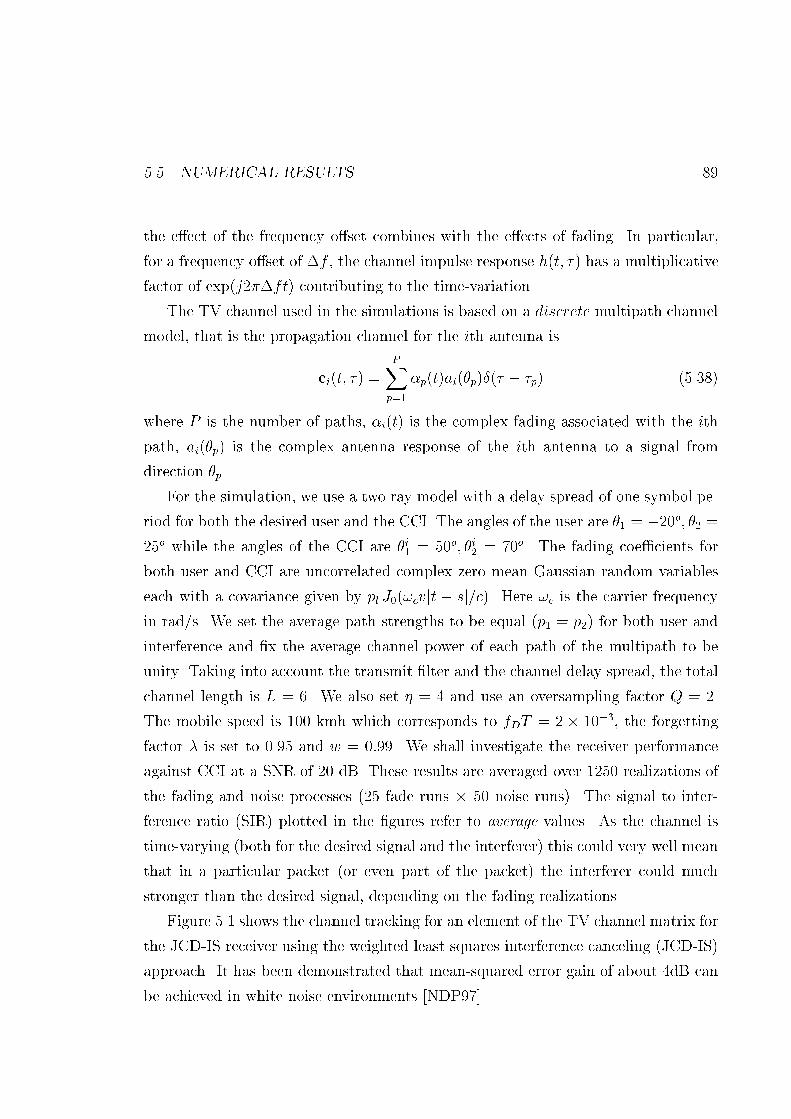
5.5. NUMERICAL RESULTS 89the e�ect of the frequency o�set combines with the e�ects of fading. In particular,for a frequency o�set of �f , the channel impulse response h(t; �) has a multiplicativefactor of exp(j2��ft) contributing to the time-variation.The TV channel used in the simulations is based on a discrete multipath channelmodel, that is the propagation channel for the ith antenna isci(t; �) = PXp=1 �p(t)ai(�p)�(� � �p) (5.38)where P is the number of paths, �i(t) is the complex fading associated with the ithpath, ai(�p) is the complex antenna response of the ith antenna to a signal fromdirection �p.For the simulation, we use a two ray model with a delay spread of one symbol pe-riod for both the desired user and the CCI. The angles of the user are �1 = �20o; �2 =25o while the angles of the CCI are �i1 = 50o; �i2 = 70o. The fading coe�cients forboth user and CCI are uncorrelated complex zero mean Gaussian random variableseach with a covariance given by pl J0(!cvjt � sj=c). Here !c is the carrier frequencyin rad/s. We set the average path strengths to be equal (p1 = p2) for both user andinterference and �x the average channel power of each path of the multipath to beunity. Taking into account the transmit �lter and the channel delay spread, the totalchannel length is L = 6. We also set � = 4 and use an oversampling factor Q = 2.The mobile speed is 100 kmh which corresponds to fDT = 2 � 10�3, the forgettingfactor � is set to 0.95 and w = 0:99. We shall investigate the receiver performanceagainst CCI at a SNR of 20 dB. These results are averaged over 1250 realizations ofthe fading and noise processes (25 fade runs � 50 noise runs). The signal to inter-ference ratio (SIR) plotted in the �gures refer to average values. As the channel istime-varying (both for the desired signal and the interferer) this could very well meanthat in a particular packet (or even part of the packet) the interferer could muchstronger than the desired signal, depending on the fading realizations.Figure 5.1 shows the channel tracking for an element of the TV channel matrix forthe JCD-IS receiver using the weighted least squares interference canceling (JCD-IS)approach. It has been demonstrated that mean-squared error gain of about 4dB canbe achieved in white noise environments [NDP97].

90 CHAPTER 5. INTERFERENCE SUPPRESSIONFigure 5.2 shows that the error rate performance of the JCD-IS receivers canbe improved if a colored Gaussian (Mahalanobis distance) metric is used instead ofa minimum euclidean distance decoding (MEDD) metric. At a target BER of 1%,using a Mahalanobis distance metric leads to a SIR improvement of at least 8 dBover the MEDD metric. The SIR improvement is less (about 3 dB) if the receiveruses an unstructured TV channel model. This �gure demonstrates the advantage ofincorporating transmit pulse shape knowledge into the channel description. Figure5.3 shows the BER of JCD-IS receivers using correct decision feedback (CDFB). Weobserve that the JCD-IS receiver using a structured channel model can achieve errorrates that are slightly better that the CDFB receiver using an unstructured channelmodel at high SIR. The analytical truncated union bound (TUB) of the BER forthe JCD-IS receiver under CDFB is also shown. The TUB is computed from theapproximate PEP expression in section 5.3. This is done by truncating the lengthof error events to about 30 symbols and error sequences with Hamming weight notmore than 6.Next, we investigate the BER performance of the proposed reduced complexityDDFSE JCD-IS receiver. From Figure 5.4, we observe that the BER performancesfor both the reduced complexity receiver and the full complexity receiver are quiteclose. The variations in the BER curve can be attributed to statistical uctuationsin the numerical runs.We end this section with a simulation scenario where the JCD-IS receiver operatesin an environment when the CCI and the user are slot-misaligned by half a time slot.This corresponds to a change in the CCI statistics in the middle of the slot where thereceiver is in the tracking mode. The �rst CCI has the original parameters as in the�rst example. The second independent CCI which appears in the middle of the slotat which the �rst CCI disappears has the following parameters : �i1 = 45�; �i2 = 65�.Figure 5.5 shows the BER of the JCD-IS and JCD-MEDD receivers. In this case bothreceivers have similar performances with the JCD-IS performing marginally better athigh SIR. However, the di�erences are quite small and, because of the statistical uctuations in the simulation results, the advantages of JCD-IS over JCD-MEDD arenot clearly indicated. As expected, both receivers do not perform as well as when

5.6. SUMMARY 91there is only one and the same CCI throughout the slot.
0 100 200 300−0.8
−0.6
−0.4
−0.2
0
0.2
real
H
No. of symbols
JCD−IC (Struct)
0 100 200 3000
0.2
0.4
0.6
0.8
1
imag
H
No. of symbols
JCD−IC (Struct)
0 100 200 300−0.8
−0.7
−0.6
−0.5
−0.4
−0.3
−0.2
−0.1
real
H
No. of symbols
JCD−IC (Unstruct)
0 100 200 3000
0.2
0.4
0.6
0.8
1
imag
H
No. of symbols
JCD−IC (Unstruct)
Figure 5.1: Plots of channel tracking performance for IS scheme with the structuredand conventional (unstructured) channel estimators.5.6 SummaryIn this chapter we described an interference suppression scheme that uses a Gaussiandecoding metric to suppress the interference. By maintaining estimates of the chan-nel and interference covariance matrix, conditioned on candidate data sequences, thealgorithm is less susceptible to error propagation. We improve the channel estimates

92 CHAPTER 5. INTERFERENCE SUPPRESSIONby incorporating the knowledge of the transmit pulse shape. The algorithm sup-presses the dimensions dominated by the interference, before detecting the desiredsignal. The pairwise error probability analysis demonstrates that the performanceof this algorithm is similar to performing detection in a lower dimensional space.The numerical results show that this is a promising scheme for uncertain channelenvironments.

5.6. SUMMARY 93
0 2 4 6 8 10 12 14 16 18 2010
−5
10−4
10−3
10−2
10−1
100
SIR (dB)
BE
R
JCD−IC (struct.) MEDD (struct.) JCD−IC (unstruct.)MEDD (unstruct.) CSI
Figure 5.2: Comparison of BER performances between JCD-IS and MEDD JCDreceivers.
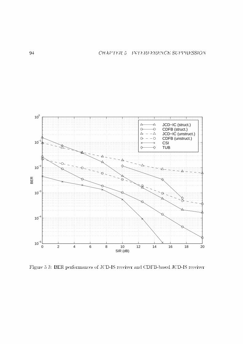
94 CHAPTER 5. INTERFERENCE SUPPRESSION
0 2 4 6 8 10 12 14 16 18 2010
−5
10−4
10−3
10−2
10−1
100
SIR (dB)
BE
R
JCD−IC (struct.) CDFB (struct.) JCD−IC (unstruct.)CDFB (unstruct.) CSI TUB
Figure 5.3: BER performances of JCD-IS receiver and CDFB-based JCD-IS receiver.

5.6. SUMMARY 95
0 2 4 6 8 10 12 14 16 18 2010
−5
10−4
10−3
10−2
10−1
100
SIR (dB)
BE
R
JCD−IC (struct.) DDFSE JCD−IC (struct.)CSI
Figure 5.4: BER performance of the reduced complexity DDFSE JCD-IS receiver.

96 CHAPTER 5. INTERFERENCE SUPPRESSION
0 2 4 6 8 10 12 14 16 18 2010
−3
10−2
10−1
100
SIR (dB)
BE
R
JCD−ICMEDD
Figure 5.5: BER performance of the JCD-IS and JCD-MEDD receivers with abruptchange in CCI in the middle of user time slot.

Chapter 6Conclusions and future WorkThe main focus of this dissertation is to understand some aspects of robust commu-nication in the presence of uncertain interference and channel fading. By studyingthis from an information theoretic perspective, we gain an understanding about ro-bust communication schemes. Using this, we develop signal processing algorithms tocommunicate reliably in uncertain environments.6.1 Thesis summaryThe mathematical description of a wireless communication environment is describedin Chapter 2. Here we give an overview of the wireless channel characteristics, de-velop a discrete-time model and the notation used in the later chapters. The maincontributions of the dissertation are contained in Chapters 3{5.Undesired interference arising from signals from outside the cell of interest, ismodeled as additive noise with an unknown distribution. In Chapter 3, we studythe problem of robust communication over a class of additive noise processes havingcovariance constraints. We �rst study this as a game-theoretic problem with mutualinformation as the pay-o� and show that Gaussian signalling and Gaussian noiseconstitute a saddlepoint to this problem. In this context, we also show that for abanded noise covariance constraint, the maximum entropy noise is the worst noisewhen we have su�cient transmit signal power. We show that this is not so for lower97

98 CHAPTER 6. CONCLUSIONS AND FUTURE WORKtransmit signal powers, and give a characterization of the worst noise when we havevery low transmit power. For robust communication, we need both a transmissionand a decoding scheme. We study the achievable rate when we use random Gaussiancodebooks and a Gaussian decoding rule when the noise covariance is known. We showthat under certain conditions on the noise process, the Gaussian rate is achievableeven with mismatched decoding. This result needs to be interpreted with caution,as it is proved that the average error probability, averaged over random transmitcodebooks, goes to zero. This is not shown for a deterministic coding scheme as inpower constrained arbitrarily varying channels [CN91]. Given this caveat, the resultshows that with a random Gaussian codebook and minimum Mahalanobis distancedecoding, the rate 12 log jKx+KzjjKzj is achievable.In Chapter 4 we study spatial diversity fading channels using an informationtheoretic approach. The utility of both transmitter and receiver spatial diversity isillustrated through the rate advantages it provides. We also analyze the performanceof OFDM in fast time-varying channels and demonstrate that we would need equal-ization (joint decoding) to achieve higher reliable information rates. This shows atrade-o� between complexity needed for equalization (time/frequency domain) andtransmission overhead.Using the insights gained in Chapter 3 and 4 on robust communication structures,we propose a joint channel-data estimation scheme with interference suppression inChapter 5. By jointly estimating the channel and the noise covariance based oncandidate data sequences, we develop a scheme suitable for uncertain channel envi-ronments. We also use the channel structure for improved channel estimation. Weanalyze the error probability of the proposed scheme and extract the properties ofthis algorithm. Numerical results based on useful channel models are also used toillustrate its performance.6.2 Future workWe conclude by discussing some interesting problems that are natural extensions ofthe work presented here.

6.2. FUTURE WORK 99In Chapter 3 we addressed the problem of robust communication in additive noisecovariance constrained noise. We showed that for a banded covariance constraint, theworst noise is the maximum entropy for su�ciently high transmit power. We alsocharacterized the worst noise for very low transmit power. To complete this problem,we need to �nd a characterization of the worst noise for intermediate signal pow-ers. We believe that this characterization will yield a parametric family of processesleading up to the maximum entropy noise at high signal powers.In Chapter 4 we examined the achievable performance for spatial diversity fadingchannels. Several open questions relevant to this topic remain unanswered. Onequestion is about the achievable rate and code-design criterion for spatially correlatedfading channels. Here one would intuitively expect that one would design codesthat transmit along the \preferred" spatial directions rather than omnidirectional(spatially white) codes. Next, an explicit form for achievable rate for time-varyingISI channels is desirable. In this thesis we have developed expressions for both quasi-static (slow time-varying) channels and for the case where we transmit using �nitesize packets and code across these packets. The capacity of a time-varying channelwould involve using large packet sizes and developing an expression for it asymptoticin the size of the transmission block. Finally, the question of the best basis fortransmission on time-varying channels is an open one. We have seen that there is rateloss associated with ignoring the ICI. One approach would be to choose a basis whichhas lower ICI and thus a lower rate loss with complexity similar to OFDM. Answersto these questions would have an in uence on the design of e�cient communicationstructures for fading channels.In Chapter 5 we develop an interference suppression algorithm suitable for fasttime-varying channels. We use a colored Gaussian decoding metric based on theestimated noise covariance matrix and e�ectively perform detection after suppressingthe interference subspace. There are several unresolved issues related to this problem.Firstly, new cost criteria for the identi�cation algorithm can be developed. Localminima would be eliminated if a convex cost criterion is chosen. Secondly, a betteranalysis for the mismatched PEP could be developed without assumption 4 in Section5.3.2. Next, reduced complexity schemes need to be investigated. Better schemes

100 CHAPTER 6. CONCLUSIONS AND FUTURE WORKto detect and handle abrupt changes in the CCI statistics (due to asynchronousinterference) need to be developed. Finally, extensions of these concepts to CDMAcould be investigated.

Appendix AAppendix to Chapter 3Lemma A.1 If X � N (0; Kx),EX[exp(�b(X � a)TA�1(X� a)=2)] = jA=bj1=2jA=b +Kxj1=2 exp(�aT (Kx +A=b)�1a=2)(A.1)Proof: We can always write X = B , where � N (0; I) and B is a nxm matrix.Here m denotes the rank of Kx. Therefore, we haveEX[12 exp(�b(X� a)TA�1(X� a))] = E [12 exp(�b(B � a)TA�1(B � a))](A.2)(a)= 1jI +BTA�1bBj1=2 exp ��aT (A�1b�A�1bB(I +BTA�1bB)�1BTA�1b)a=2�(b)= jA=bj1=2jA=b+Kxj1=2 exp(�aT (Kx +A=b)�1a=2)where (a) follows from � N (0; I) and (b) uses the matrix inversion lemma and thefacts: Kx = BBT , jI + UV j = jI + V U j [Hay91]. �Lemma A.2 (Lemma 3.9) If X(n) � N (0; Kx) and is independent of Y(n), then wehave, E [exp(12Y(n)T (Kx +Kz)�1Y(n)� 12(Y(n) �X(n))TK�1z (Y(n) �X(n)))] (A.3)= exp(�12 log(jKx +Kzj=jKzj))101

102 APPENDIX A. APPENDIX TO CHAPTER 3Proof of Lemma 3.9:E [exp(12Y(n)T (Kx +Kz)�1Y(n) � 12(Y(n) �X(n))TK�1z (Y(n) �X(n)))] (A.4)= E Y [e 12y(n)T (Kx+Kz)�1y(n)E XjY [e� 12 (y(n)�x(n))TK�1z (y(n)�x(n))jY(n)]](a)= E Y [e 12y(n)T (Kx+Kz)�1y(n)E X [e� 12 (y(n)�x(n))TK�1z (y(n)�x(n))]](b)= E Y [ jKzj1=2jKx +Kzj1=2 ]= e� 12 log jKx+Kz jjKzjwhere (a) follows from the fact that X(n) and Y(n) are independent, (b) follows fromLemma A.1. �Lemma A.3 (Lemma 3.10) If X(n) � N (0; Kx) and is independent of Z(n), andE [Z(n)Z(n)T ] = Kz > 0, then we have,Pr[ 12nZ(n)TK�1z Z(n) > 12n(Z(n) +X(n))T (Kx +Kz)�1(Z(n) +X(n)) + �] (A.5)� (1� �)exp(�n �28 ) + �Proof of Lemma 3.10:Pr[ 12nz(n)TK�1z z(n) > 12n(z(n) + x(n))T (Kx +Kz)�1(z(n) + x(n)) + �jz(n)] (A.6)(a)� E [e ( 12z(n)TK�1z z(n)� 12 (z(n)+x(n))T (Kx+Kz)�1(z(n)+x(n))�n�)](b)= e�n �e 2z(n)TK�1z z(n)E X [e� 2 (z(n)+x(n))T (Kx+Kz)�1(z(n)+x(n))](c)= e�n �e 2z(n)TK�1z z(n) j(Kx +Kz)= j1=2jKx + (Kx +Kz)= j1=2 e� 12z(n)T (Kx+(Kx+Kz)= )�1z(n)where (a) follows from the Cherno� bound, is the Cherno� parameter, (b) followsfrom the independence ofX(n) & Z(n), and (c) follows from Lemma A.1. Let us de�ne,E(n; ; z(n)) = �+ 12n log( jKx + (Kx +Kz)= jj(Kx +Kz)= j ) (A.7)� 12nz(n)T ( K�1z � (Kx + (Kx +Kz)= )�1)z(n)

103Hence we have the RHS of (A.6) given by e�nE(n; ;z(n)). We can rewrite E(n; ; z(n))as, E(n; ; z(n)) = �+ 12n nXi=1 log(1 + 1 + �i ) (A.8)� 12nz(n)T ( K�1z � (Kx + (Kx +Kz)= )�1)z(n)where �i = 1=�i(K�1=2z KxK��=2z ).E(n; ; z(n)) (a)� � + 12n nXi=1 1 + + �i � (A.9)12nz(n)T ( K�1z � (Kx + (Kx +Kz)= )�1)z(n)(b)= � + 1 + 1 12ntrace([ K�1z � (Kx + (Kx +Kz)= )�1]Kz)�12nz(n)T ( K�1z � (Kx + (Kx +Kz)= )�1)z(n)where in (a) we have used log(1 + x) � x1+x for x � 0 and (b) is due toPni=1 1+ +�i = 1 +1trace([ K�1z � (Kx + (Kx +Kz)= )�1]Kz).Let A = f~z(n) : j 1nz(n)TK�1z z(n) � E [ 1nz(n)TK�1z z(n)]j < �=2; j 1nz(n)T (Kx(1 + ) +Kz)�1)z(n) � E [ 1nz(n)T (Kx(1 + ) +Kz)�1z(n)]j < �=2� 1ntrace([ K�1z � (Kx + (Kx +Kz)= )�1]Kz)j < �g. From C1 and C1 we have Pr[A] > 1� � for all n � N(�). If weevaluate E(n; ; z(n)) when ~z(n) 2 A and denote it by E(n; ; z(n)jA) we have,E(n; ; z(n)jA) (a)� �� 2 [�� ] (A.10)= 2 [�� ](b)� �28where (a) follows because ~z(n) 2 A and (b) follows by choosing � �. The resultfollows by using (A.6), (A.10) = �2(1+�) , and Pr[A] > 1� �. �

Appendix BDetails of Proposition 4.1B.1 Proof outlineProposition B.1 If H(k) = [h1(k); : : : ;hN(k)] 2 CM�N and hl(k) � CN (0; I); l =1; : : : ; N , are i.i.d. then limN!1PNj 6=i;j=1 jhHi (k)hj(k)N j2 = 1, almost surely.Proof: For brevity we will suppress the time index k and denote Vj = jhHi hj j2N � 1.Let us examine,E [ 1N Xj 6=i Vj]4 = 1N4 E [Xk1 Xk2 Xk3 Xk4 Vk1Vk2Vk3Vk4 ] (B.1)(a)= 1N4f(�n4 � 6�n3 + 11�n2 � 6�n)E [Vk1Vk2Vk3Vk4] +(6�n3 � 18�n2 + 12�n)E [V 2k1Vk3Vk4 ]+�nE [V 4k1 ] + (3�n2 � 3�n)E [V 2k1V 2k2] + (4�n2 � 4�n)E [V 3k1Vk2 ]gwhere �n = N � 1, (a) follows by the expansion of the product and using the i.i.d.property, and the notation Vk1Vk2Vk3Vk4 is shorthand for the case k1 6= k2 6= k3 6= k4.Note that E jV j2 = 1, E jV j4 = 2 for V � CN (0; 1) having i.i.d. real and imaginaryparts. Using this and the i.i.d. property of hj � CN (0; I) we can show after some104

B.1. PROOF OUTLINE 105algebra (see Appendix B.2) that,E [Vk1Vk2Vk3Vk4] = E [(hHi hi=N � 1)4] = O( 1N2 ) (B.2)E [V 2k1Vk3Vk4] = E [(hHi hi=N)2(hHi hi=N � 1)2] = O( 1N )E [V 4k1 ] = O(1)E [V 2k1V 2k2] = O(1)E [V 3k1Vk2] = O(1)where h(n) = O(g(n)) means limsupn!1jh(n)g(n) j <1 [Wil91]. Using (B.2) in (B.1) weobtain, E [Pj 6=i VjN ]4 = O( 1N2 ) (B.3)which implies that PN E [Pj 6=i VjN ]4 <1. This means that Pj 6=i Vj=N ! 0; a:s: usingTheorem 6.5 in [Wil91]. Thus we have,limN!1Xj 6=i 1N jhHi hjj2 = limN!1(N � 1)=N = 1; a:s: (B.4)�To prove (4.10) let us de�ne WN = log(1 + (jjhijj2)2P=Njjhijj2�2+(Pj 6=i jhHi hj j2)P=N ). We haveshown in (4.9) that WN converges almost surely. Notice that,WN � log(1 + jjhijj2P=N�2) (a)� jjhijj2P=N�2 (B.5)where (a) follows because log(1 + x) � x for x � 0. This can be seen by de�ningg(x) = x� log(1+x) and noticing that g(0) = 0; dg(x)=dx = x=(1+x) � 0 for x � 0.Hence the inequality holds as g(x) is an increasing function. Using (B.11) we have,EW 2N � (P=�2)2E (jjhijj2=N)2 = (1 + 1=N)(P=�2)2 � 2(P=�2)2; 8N: (B.6)Hence using Theorems 13.3(a) and 13.7 in [Wil91] fWNg is uniformly integrable andhence limN!1 EWN = E limN!1WN giving us (4.10).

106 APPENDIX B. DETAILS OF PROPOSITION 4.1B.2 Proof detailsIn this section we outline the algebra to show (B.2). Using Vj = 1N jhHi hjj2 � 1 wehave,E [Vk1Vk2Vk3Vk4] = E [(jhHi hk1j2=N � 1)(jhHi hk2j2=N � 1)(jhHi hk3 j2=N � 1) (B.7)(jhHi hk4 j2=N � 1)](a)= E �jhHi hk1 j2jhHi hk2 j2jhHi hk3 j2jhHi hk4 j2=N4� 4jhHi hk1j2jhHi hk2j2jhHi hk3j2=N3 + 6jhHi hk1 j2jhHi hk2 j2=N2�4jhHi hk1 j2=N + 1where (a) follows by using the fact that fhjg are i.i.d. and k1 6= k2 6= k3 6= k4. Now wehave, E jhHi hk1 j2jhHi hk2 j2jhHi hk3 j2jhHi hk4 j2 =Pl1Pl2Pl3Pl4 E jhil1 j2jhil2 j2jhil3j2jhil4 j2by using the fact that E [hjl] = 0, E [jhjlj2] = 1 and hk1 ;hk2 ;hk3;hk4 are inde-pendent. In a similar manner we can show that, E jhHi hk1 j2jhHi hk2 j2jhHi hk3j2 =Pl1Pl2Pl3 E jhil1 j2jhil2 j2jhil3 j2, E jhHi hk1 j2jhHi hk2 j2 =Pl1Pl2 E jhil1j2jhil2j2 andE jhHi hk1j2j =Pl1 E jhil1 j2. Thus using (B.7) we get,E [Vk1Vk2Vk3Vk4] = E [Xl jhilj2=N � 1]4 (B.8)Now, from a combinatorial count and using E [jhilj2] = 1 and E [jhilj4] = 2 we have,Xl1;::: ;l4 1N4 E [jhil1 j2jhil2 j2jhil3 j2jhil4 j2] = N4 � 6N3 + 11N2 � 6NN4 E �jhil1 j2jhil2 j2(B.9)jhil3 j2jhil4j2�+ 6N3 � 18N2 + 12NN4E jhil1 j4jhil2 j2jhil3 j2 +O(1=N2)= 1 + 6=N +O(1=N2)Similarly we have,Xl1 Xl2 Xl3 1N3 E [jhil1 j2jhil2 j2jhil3 j2] = (N3 � 3N2 + 2N)N3 E jhil1 j2jhil2 j2jhil3j2 (B.10)+(3N2 � 3N)N3 E jhil1j4jhil2 j2 +O(1=N2)= 1 + 3=N + O(1=N2)

B.2. PROOF DETAILS 107Xl1 Xl2 1N2 E jhil1 j2jhil2 j2 = (N(N � 1))N2 E jhil1 j2jhil2j2 + NN2 E jhil1 j4 (B.11)= 1 + 1=NXl1 E jhil1 j2j=N = 1 (B.12)Thus using (B.9{B.12) in (B.7) we get, E [Vk1Vk2Vk3Vk4 ] = O(1=N2).To show that E [V 2k1Vk2Vk3 ] = O(1=N), let us consider,E [V 2k1Vk2Vk3 ] = E [(jhHi hk1j2=N � 1)2(jhHi hk2j2=N � 1)(jhHi hk3 j2=N � 1)] (B.13)(a)= E �jhHi hk1j4jhHi hk2j2jhHi hk3j2=N4 � 2jhHi hk1j2jhHi hk2j2jhHi hk3j2=N3� 2jhHi hk1 j4jhHi hk2 j2=N3 + jhHi hk1j4=N2+5jhHi hk1 j2jhHi hk2 j2=N2 � 4jhHi hk1 j2=N + 1where (a) follows by using the fact that fhjg are i.i.d. and k1 6= k2 6= k3. We have,1N4 E [jhHi hk1j4jhHi hk2j2jhHi hk3j2] = 1N4 Xl1;::: ;l6 E h�il1hil2h�il3hil4 jhil5 j2jhil6 j2 (B.14)Ehk1l1h�k1l2hk1l3h�k1l4(a)= 1N4 Xl5;l6 (Xl1 E [jhil1 j4jhil5 j2jhil6 j2]E [jhk1l1 j4]+ 2 Xl1;l3 6=l1 E [jhil1 j2jhil3 j2jhil5 j2jhil6 j2]E [jhk1l1 j2jhk1l3 j2])(b)= 2 Xl1;::: ;l4 E jhil1 j2jhil2 j2jhil3 j2jhil4 j2(c)= 2(1 + 6=N) +O(1=N2)where (a) follows from the fact that hkl are i.i.d., (b) by using E jhklj2 = 1; E jhklj4 = 2

108 APPENDIX B. DETAILS OF PROPOSITION 4.1and (c) from (B.9). Similarly we have,E [ jhHi hk1 j4jhHi hk2 j2N3 ] = Xl1;::: ;l5 1N3 E [h�il1hil2h�il3hil4 jhil5 j2] (B.15)E [hk1l1h�k1l2hk1l3h�k1l4 ]E [jhk2l5 j2]= 1N3 Xl5 (Xl1 E [jhil1 j4jhil5 j2]E [jhk1l1 j4]+2 Xl1;l3 6=l1 E [jhil1j2jhil3 j2jhil5 j2]E [jhk1l1 j2jhk1l3 j2])= 2 Xl1;::: ;l3 E jhil1 j2jhil2 j2jhil3 j2 = 2(1 + 3=N) +O(1=N2)E [jhHi hk1j4=N2] = Xl1;::: ;l4 E [h�il1hil2h�il3hil4]E [hk1l1h�k1l2hk1l3h�k1l4 ]=N2 (B.16)= 1N2 (Xl1 E [jhil1j4]E [jhk1l1 j4]+2 Xl1;l3 6=l1 E [jhil1j2jhil3 j2]E [jhk1l1 j2jhk1l3 j2])= 2Xl1;l2 E jhil1 j2jhil2 j2 = 2(1 + 1=N)Using (B.9{B.12) and (B.14{B.16) in (B.13) we get E [V 2k1Vk2Vk3] = O(1=N). Bysimilar algebra we can show the other relations given in (B.2). In these expressionswe use similar combinatorial count arguments and the fact that for hil � CN (0; 1),E jhilj2p is a known �nite constant for p = 1; : : : ; 4.

Appendix CDetails of Proposition 4.3Proposition C.1 If limN!1PNi=1Pij=1 jUjj2(C=N2) = � andlimN!1max1�i�NPij=1 jUjj2(C=N2) = 0, thenlimN!1 NXi=1 log(1 + iXj=1 jUjj2(C=N2)) = �;where C is any constant.Proof: Let bi;N =Pij=1 jUjj2(C=N2) hence limN!1max1�i�N jbi;N j = 0. Thus 8� >0 there is N� s.t., jbi;N j < �; 8N � N�. Now, using the fact that j log(1+ z)� zj � jzj2for jzj � 1=2 (see for e.g. [Wil91], 18.3(c)). Using � < 1=2; s:t:; jbi;N j < � < 1=2 8N �N� we have j log(1 + bi;N)� bi;N j � �2, and hence by letting � = 1=N we obtainNXi=1 bi;N � (1=N) � NXi=1 log(1 + bi;N ) � NXi=1 bi;N + (1=N) (C.1)Hence by a sandwich argument we have the desired result. �Proposition C.2 If Ui � CN (0; 1) is i.i.d. then limN!1PNi=1Pij=1 jUjj2(C=N2) =C=2; a:s: 109

110 APPENDIX C. DETAILS OF PROPOSITION 4.3Proof: By exchanging the two �nite sums over i and j we have,NXi=1 iXj=1 jUjj2(C=N2) = NXj=1 NXi=j jUjj2(C=N2) = NXj=1(N � j + 1)jUjj2C=N2 (C.2)= C " 1N NXj=1 jUjj2 + 1N2 NXj=1 jUjj2 � 1N NXj=1 jUjj2(j=N)#Now consider,E [ 1N NXj=1(jUjj2(j=N)� 1=2)]4 (a)= 1N4 NXj=1 E [jUjj2(j=N)� 1=2]4 + 1N4 Xj1 Xj2 6=j1 (C.3)E [jUj1j2(j1=N)� 1=2]2E [jUj2j2(j2=N)� 1=2]2(b)= O(1=N2)where (a) follows by the i.i.d. nature of fUjg and (b) follows because E [jUjj2]4 <1.Hence as in the proof of Proposition B.1, by using the Borel-Cantelli lemma we get,limN!1 1N NXj=1(jUjj2(j=N)� 1=2) = 0; a:s: (C.4)Thus limN!1 1N PNj=1 jUjj2(j=N) = 1=2 a:s: Using this and limN!1Pj jUjj2=N =1 a:s: (SLLN), in (C.2) we have the result. �By using Propositions C.1 and C.2 we obtain,limN!1Xi log(1 + P�2N2 iXj=1 jUjj2) = P=2�2; a:s: (C.5)It is easy to show that fPi log(1 + P�2N2 Pij=1 jUjj2)g is uniformly integrable (usingarguments similar to that used in Appendix B.1) and thus we can exchange limitsand expectation and obtain the result of Proposition 4.3.

Appendix DWSSUS channel calculations forSection 4.3.3In this section we outline the algebra leading to (4.42) and (4.43).If qs = [1; : : : ; exp(j2�s(n� 1)=n)]T we can show using (4.32) that(Hqs)r = ��1Xl=0 h(r; l)exp(j2�s((r � l))n=n) (D.1)where ((�))n denotes modulo-n addition. Hence as G(m; s) = 1nqHmHqs andexp(j2�s((r � l))n=n) = exp(j2�s(r � l)=n) we can write,G(m; s) = 1n n�1Xr=0 ��1Xl=0 h(r; l)exp(j2�r(s�m)=n)exp(�j2�sl=n) (D.2)Now, using the WSSUS assumption we have E [h(r1; l1)h(r2; l2)] = rh(r1�r2)�(l1� l2)and using this and (D.2) we get (4.42).Next, we outline the steps leading to (4.43). From (D.2) it is clear that gm =[G(m; 0); : : : ; G(m;n� 1)]T � CN (0;R1) where R1 is determined from (4.42). Sim-ilarly as �gm � CN (0;R2), our problem in evaluating (4.41) reduces to �ndingE log(�2 + P jjwjj2) for w � CN (0;R). To this end we can write wHw = HR =~ � ~ , where � CN (0; I), ~ � CN (0; I) and R = U�UH is its eigendecompo-sition. Thus wHw = Pq �qj qj2 where f�g are the eigenvalues of R. As f ~ g are111

112 APPENDIX D. WSSUS CHANNEL CALCULATIONS FOR SECTION 4.3.3independent Gaussians we can write the characteristic function of wHw as�(!) =Yq 11� j!�q (a)= Xq �q1� j!�q (D.3)where we have assumed distinct eigenvalues to get the partial fraction expansion (a).Thus the probability density function of wHw is,fwHw(�) =Xq (�q=�q)exp(��=�q); � � 0: (D.4)Hence, E [log(�2 + P jjwjj2) =Xq �q Z 10 1�q log(�2 + P�2) exp(��=�q)d� (D.5)Using the fact that R10 1�q log(�2+P�2) exp(��=�q)d� = � exp(�2=P�q)Ei(��2=P�q)[GR94] where Ei(�) is the exponential integral function we obtain (4.43).
Appendix ECalculation of Hessian for Section5.2.2We de�ne@vec(U)@vec(R)T = [vec(@(U)@R11 ); : : : ; vec( @(U)@R1N ); : : : ; vec( @(U)@RN1 ); : : : ; vec( @(U)@RNN )] (E.1)where R is a N �N matrix, and Rmn denotes its (m;n)th element. To calculate V22we need the following lemma.Lemma E.1 @vec(R�1)vec(R)T = �R�1 R�1 (E.2)Proof: As R�1R = I, we have by di�erentiating w.r.t. Rmn,@R�1@Rmn = �R�1EmnR�1 = �(R�1em)(R�1en)T (E.3)where em is the mth unit vector. Hence as,vec( @R�1@Rmn ) = �(R�1en) (R�1em) (E.4)and using (E.1) we get the desired result. �Claim E.1 V22jE k[��T ]=R = R�1 R�1 (E.5)113

114 APPENDIX E. CALCULATION OF HESSIAN FOR SECTION 5.2.2Proof: From (5.14) we get,V22 = �@(vec(R�1E k[��T ]R�1))@vec(R)T + @(vec(R�1))@vec(R)T (E.6)Clearly the second term of (E.6) is given by Lemma E.1. For the �rst term we have,@(R�1E k[��T ]R�1)@Rmn = E k[@(R�1)@Rmn ��TR�1 +R�1��T @(R�1)@Rmn ] (E.7)(a)= �E k[(R�1em)(R�1en)T��TR�1+R�1��T (R�1em)(R�1en)T ]where (a) follows from (E.3). When we evaluate (E.7) for E k[��T ] = R we obtain,vec(@(R�1E k[��T ]R�1)@Rmn ) = �2(R�1en) (R�1em) (E.8)Using (E.8), Lemma E.1 and (E.1) we get the desired result. �

Appendix FAppendix to Section 5.3.2F.1 Covariance matrix of parametric vector chan-nelIn this appendix, we shall derive the covariance matrix of the vector channel based onthe parametric channel model where the propagation channel is composed of discretemultipaths arriving at the receiver array with di�erent angles of arrival and delays.We start by writing the multichannel receiver output asy(t) =Xn sn PXp=1 a(�p)�p(t)g(t� nT � �p)! (F.1)By fractionally sampling (F.1) to obtain the su�cient statistics at a rate Q=T , weobtain y(kT + qT=Q) = L�1Xm=0 sk�mh(kT + qT=Q;mT )where h(kT + qT=Q;mT ) = PXp=1 a(�p)�p(kT + qT=Q)g(mT + qT=Q� �p)= A(�)D(kT + qT=Q)g(mT + qT=Q; � ) (F.2)= �gT (mT + qT=Q; � ) �A(�)��(kT + qT=Q) (F.3)115

116 APPENDIX F. APPENDIX TO SECTION 5.3.2The de�nitions for the terms in (F.2)-(F.3) are as followsA(�) = [a(�1); a(�2); � � � ; a(�P )]D(kT + qT=Q) = diag[�1(kT + qT=Q); �2(kT + qT=Q); � � � ; �P (kT + qT=Q)]g(mT + qT=Q; � ) = 2666664 g(mT + qT=Q� �1)g(mT + qT=Q� �2)...g(mT + qT=Q� �P )3777775�(kT + qT=Q) = [�1(kT + qT=Q); �2(kT + qT=Q); � � � ; �P (kT + qT=Q)]Tand where � is the Khatri-Rao (column-wise) matrix product (see Appendix G).Our goal is to �nd the covariance matrix of hk. It can be veri�ed that hk =vec(HTk ) whereHk = 26666664 �gT (0; � ) �A(�)��(kT ) � � � hgT ((Q� 1) TQ ;� ) �A(�)i�(kT + (Q� 1) TQ )�gT (T; � ) �A(�)��(kT ) � � � hgT (T + (Q� 1) TQ ;� ) �A(�)i�(kT + (Q� 1) TQ )... ... ...�gT ((L � 1)T; � ) �A(�)��(kT ) � � � hgT ((L� 1)T + (Q� 1) TQ ;� ) �A(�)i�(kT + (Q� 1) TQ ) 37777775Let Gi = 266664 gT (iT=Q; � )gT (T + iT=Q; � )� � �gT ((L� 1)T + iT=Q; � )
377775This de�nition allows us to write Hk as� [G0 �A(�)]�(kT ); [G1 �A(�)]�(kT + TQ); � � � ; [GQ�1 �A(�)]�(kT + (Q� 1)TQ) �Recall hk = vec(HTk ) = P1vec(Hk) where P1 is a permutation matrix that reordersthe rows of vec(Hk) and is given byP1 = 2664 IQ eT1...IQ eTML 3775MQL�MQL

F.1. COVARIANCE MATRIX OF PARAMETRIC VECTOR CHANNEL 117where ei is theML�1 unit vector with a one in the ith position and zero elsewhere.Now vec(Hk) = F2666664 �(kT )�(kT + T=Q)...�(kT + (Q� 1)T=Q)3777775 (F.4)where F = 2666664 G0 �A(�) G1 �A(�) . . . GQ�1 �A(�)3777775MLQ�PQBy de�ning another PQ� PQ permutation matrix P2P2 = 2664 IP eT1...IP eTQ 3775PQ�PQwhere ei now denotes a Q� 1 unit vector such thatP2 2666664 �(kT )�(kT + T=Q)...�(kT + (Q� 1)T=Q)
3777775 = �k (F.5)In (F.5), �k denotes the fading variables arranged in order of the path index �rst, i.e.�k = [�1(kT ); �1(kT + T=Q); � � � ;�1 (kT + (Q� 1)T=Q); � � � ; �P (kT ); �P (kT + T=Q); � � � ; �P (kT + (Q� 1)T=Q)]TUsing (F.4) and (F.5), we obtain the linear model for hk as a function of �khk = P1FP2�k (F.6)

118 APPENDIX F. APPENDIX TO SECTION 5.3.2The cross-covariance matrix of hk can now be calculated asE (hkhHk+n) = P1FP2R�k�k+n PT2FHPT1 (F.7)For the case of independent Rayleigh fading between paths,R�k�k+n = � �n (F.8)where � is the diagonal P � P matrix containing the powers of the multipaths andthe Q �Q matrix �n describes the temporal correlation of each path at lag nT andits ijth component is [�n]ij = J0(!D(jnj+ ji� jj=Q))where !D = 2� fd T is the normalized Doppler angular frequency and fd is the Dopplerfrequency in Hz. Using (F.7) and (F.8), the cross-covariance matrix is given byRhkhk+n = P1FP2 (� �n)PT2FHPT1 (F.9)This completes the derivation of the (cross)-covariance matrix of the hk.F.2 Covariance matrix of channel estimation errorIn this appendix, we shall investigate the channel estimation error vector for theRLS channel updates. Our objective is to obtain an (asymptotic) expression for thecovariance matrix of the channel estimation error vector for the purpose of computingthe PEP. We shall also show that the channel estimation error vector is approximatelyindependent of the true channel vector under quasi-static channel conditions over thelength of typical error events.The channel estimation error vector is de�ned as�hk = hk � hk = �hk � E hk�| {z }�hk +�E hk � hk�| {z }g�hkThe vector �hk is the channel estimation noise vector and it quanti�es the deviationof the channel estimate from its mean value as a result of noise perturbations. On

F.2. COVARIANCE MATRIX OF CHANNEL ESTIMATION ERROR 119the other hand, the vector f�hk is the channel lag vector and is used to quantify thetracking error inherent in the adaptive algorithm as a result of channel dynamics. Weshall investigate these quantities separately. We shall also see that both vectors arestatistically independent so that the sum of their covariance matrices give the totalcovariance matrix of �hk.F.2.1 Channel estimation noise vector �hkThe RLS channel estimate ishk = Gck = G"Xi �k�iBHi R�1z Bi#�1 "Xi �k�iBHi R�1z yi# (F.10)Let k = �Pi �k�iBHi R�1z Bi��1. Since yi = Bici + zi and taking expectation of(F.10) over the noise, E hk = GkXi �k�iBHi R�1z BiciThe channel estimation noise vector can now be written as�hk = GkXi �k�iBHi R�1z zi (F.11)It is clear from (F.11) that �hk has zero mean. The covariance matrix isCov ��hk� = E ��hk �hHk � = Gk Xi �2(k�i)BHi R�1z Bi!kGT (F.12)where we have made use of weak temporal correlation of zi in assumption 3 in section5.3.5.3.2 to obtain the second equality. Since we are concerned with the stationaryproperties of the channel error statistics in the tracking mode and assuming ergodicity,the large sample limit (asymptotic) covariance matrix is sought. HenceR�h = limk!1Gk Xi �2(k�i)BHi R�1z Bi!kGT= G limk!1Xi �2(k�i)BHi R�1z Bi!GT
120 APPENDIX F. APPENDIX TO SECTION 5.3.2where = limk!1k. By the continuity of the matrix inverse mapping and providedthe limit exist, = limk!1" kXi �k�iBHi R�1z Bi#�1= " limk!1 kXi �k�iBHi R�1z Bi#�1= " limk!1 kXi �k�iGT (s�i IMQ)R�1z �sTi IMQ�G#�1(a)= " limk!1 kXi �k�iGT �s�i sTi R�1z �G#�1(b)= " 1Xi �iGT �E (s�i sTi )R�1z �G#�1(c)= � Es1� �GT �IL R�1z �G��1 (F.13)where equality (a) follows from the identity (G.3) in Appendix G, equality (b) followsfrom ergodicity1 and (c) follows from an IID assumption of the user data with E jskj2 =Es. It is readily shown thatlimk!1 kXi �2(k�i)BHi R�1z Bi = Es1� �2GT �IL R�1z �G (F.14)Using (F.13) and (F.14), we haveR�h = 1� �Es(1 + �)G hGT �IL R�1z �Gi�1GT (F.15)F.2.2 Channel lag error vector f�hkIn this section, we shall derive the asymptotic covariance matrix of the channel lagerror vector f�hk. The approach taken here follows closely the tracking error analysis1A factor of 1k has been implicitly assumed to be included in (a) before taking the limit. Thisfactor cancels out in the expression for Cov ��hk� and does not a�ect the �nal asymptotic expression.

F.2. COVARIANCE MATRIX OF CHANNEL ESTIMATION ERROR 121in [EF86]. If the variations of the channel is slow compared to the memory of thealgorithm, then it can be shown that [EF86]f�hk = � f�hk�1 � (hk � hk�1) (F.16)Taking the z-transform of (F.16) givesf�h(z) = z�1 � 11� �z�1h(z) (F.17)We can interpret equations (F.16) and (F.17) as the channel lag error vector beingthe output of a linear time-invariant �lter. The power spectrum of f�h can now becalculated as Sg�h(z) = � z�1 � 11� �z�1�� z � 11� �z�Sh(z) (F.18)where Sh(z) is the power spectrum of the true channel.Using (F.18), the cross-covariance matrix of f�h can be readily calculated asE �f�hkf�hHk+n� = 12 � Z ��� 2� 2 cos!1 + �2 � 2� cos!Sh(ej!) ej n! d ! (F.19)In particular, we shall �nd the covariance (at zero lag) of f�hk under a parametricmultipath Rayleigh fading channel model. Using (F.9), it is easily established thatSh(ej!) = P1FP2 �� �(ej!)�PT2FHPT1where �mn(ej!) = 8<: 2 ej!(jm�nj=Q)!Dp1�!2=!2D j!j < !D0 j!j � !D m;n = 1; 2; � � � ; Q: (F.20)and where !D = 2 � fd T is the normalized Doppler angular frequency. Using (F.20),the covariance matrix of f�hk can now be found asRg�h = P1FP2�� � 12 � Z ��� 2� 2 cos!1 + �2 � 2� cos!�(ej!) d !��PT2FHPT1 (F.21)

122 APPENDIX F. APPENDIX TO SECTION 5.3.2F.2.3 Total channel estimation error covarianceUsing (F.11) and (F.16), it is easy to see that �hk and f�hk are independent. Thetotal channel estimation error covariance is thus given by the sum of their covariancesR�h = R�h +Rg�h (F.22)where R�h and Rg�h are given by (F.15) and (F.21) respectively. This completesthe derivation of the channel estimation error covariance matrix. Equation (F.16)indicates that the total channel estimation error vector �hk is not temporally inde-pendent. However assumption 4 in Section 5.35.3.2 implies that �h dominates f�hand thus we can approximate �hk as an IID process.

Appendix GResults on Kronecker productsThe results summarized here can be found in [Bre78], Table II (T2.4,T2.6,T2.13,T2.14).Here R is a real symmetric matrix.(R�1 R�1)�1 = RR (G.1)(RR)vec(U) = vec(RUR) (G.2)(AD)(FU) = (AF) (DU) (G.3)If the eigenvalues of M are f kg and the eigenvalues of N are f�kg then we have,eig(NM) = i�k (G.4)If U is (t� u) and F is (q � u), the Khatri-Rao product is denoted by F �U and isde�ned [Bre78] as, F �U 4= [F1 U1;F2 U2; : : : ;Fu Uu] (G.5)where Fi denotes the ith column of matrix F. The property used from [Bre78] (TableIII, T3.13), vec(AVD) = (DT �A)vecd(V) (G.6)if V is diagonal and vecd(�) denotes the vector formed by the diagonal elements ofthe matrix. 123

Bibliography[Bar87] M. J. Barrett. Error Probability for Optimal and Suboptimal QuadraticReceivers in Rapid Rayleigh Fading Channels. IEEE Journal on SelectedAreas in Communications, SAC(2):302{304, 1987.[BC96] C R. Baker and I.-F Chao. Information Capacity of channels with par-tially unknown noise. I. �nite dimensional channels. SIAM Journal Ap-plied Math., 56(3):946{963, June 1996.[Bla57] N M. Blachman. Communication as a game. In Proceedings WesconConference, pages 61{66, August 1957.[BM97] Gregory E. Bottomley and Karl Molnar. Interference cancellation forimproved channel estimation in array processing MLSE receivers. InProc.IEEE Vehicular Technology Conference, pages 140{144, May 1997.[Bre78] John W. Brewer. Kronecker products and Matrix Calculus in SystemTheory. IEEE Transactions on Circuits and systems, 25(9):772{781,September 1978.[BRP96] Tibor Boros, Gregory Raleigh, and Mike Pollack. Adaptive space-time equalization for rapidly fading communication channels. InProc.GLOBECOM, pages 984{989, 1996.[BS92] P. Balaban and J. Salz. Optimum diversity combining and equalizationin digital data transmission with applications to cellular mobile radio.IEEE Transactions on Communications, 40:885{894, May 1992.124

BIBLIOGRAPHY 125[CDS96] L J. Cimini, Babak Daneshrad, and N R. Sollenberger. Clustered OFDMwith transmitter diversity and coding. In GLOBECOM, pages 703{707,1996.[CH92] J. K. Cavers and P. Ho. Analysis of the error performance of trellis-coded modulations in Rayleigh-fading channels. IEEE Transactions onCommunications, 40(1):74{83, January 1992.[Cio94] J M. Cio�. Digital data communications. In preparation, book to bepublished, notes for class EE 379, Stanford University, 1994.[CN91] I. Csiszar and P. Narayan. Capacity of the Gaussian arbitrarily varyingchannel. IEEE Transactions on Information Theory, 37(1):18{26, Jan1991.[CT88] Thomas M. Cover and Joy A. Thomas. Determinant inequalities via In-formation Theory. SIAM Journal of Matrix Analysis and it Applications,9:384{392, 1988.[CT91] Thomas M. Cover and Joy A. Thomas. Elements of Information Theory.John Wiley and Sons, Inc., New York, 1991.[CTVTB97] G. Caire, G. Taricco, J. Ventura-Traveset, and E. Biglieri. A multiuserapproach to narrowband cellular communications. IEEE Transactionson Information Theory, 43(5):1503{1517, September 1997.[DHH89] A. Duel-Hallen and C. Heegard. Delayed decision-feedback sequence es-timation. IEEE Transactions on Communications, 37(5):428{436, May1989.[Din97] Z. Ding. Multipath channel identi�cation based on partial system infor-mation. IEEE Transactions on Signal Processing, 45(1):235{240, Jan.1997.

126 BIBLIOGRAPHY[DNP98] Suhas N. Diggavi, Boon Chong Ng, and A. Paulraj. Joint channel-dataestimation and interference suppression. In International Conference onCommunications ICC, pages 465{469, June 1998.[Dob59] R L. Dobrushin. Optimum information transmission through a channelwith unknown parameters. Radioteck. Elektron., 4(2):1951{1956, De-cember 1959.[DP97] Suhas N. Diggavi and A. Paulraj. Performance of multisensor adaptiveMLSE in fading channels. In Proc.IEEE Vehicular Technology Confer-ence, pages 2148{2152, May 1997.[Ede89] A. Edelman. Eigenvalues and Condition numbers of random matrices.PhD thesis, Massachusetts Institute of Technology, Cambridge, MA,1989.[EF86] E. Eleftheriou and D. Falconer. Tracking properties and steady-stateperformance of RLS adaptive �lter algorithms. IEEE Trans. ASSP,ASSP-34(5):1097{1110, Oct. 1986.[Fan50] Ky Fan. On a theorem of Weyl concerning the eigenvalues of linear trans-formations II. Proceedings National Academy of Sciences U.S., 36:31{35,1950.[For72] G. David Forney. Maximum-Likelihood Sequence Estimation of DigitalSequences in the Presence of Intersymbol Interference. IEEE Transac-tions on Information Theory, 18:363{378, May 1972.[Fos96] G.J. Foschini. Layered space-time architecture for wireless communica-tion in a fading environment when using multi-element antennas. BellLabs Technical Journal, 1(2):41{59, September 1996.[Gol94] A. Goldsmith. Design and performance of high-speed communicationsystems over time-varying radio channels. PhD thesis, University ofCalifornia, Berkeley, CA., 1994.

BIBLIOGRAPHY 127[GR94] I.S. Gradshteyn and I.M. Ryzhik. Table of Integrals, Series and Products.Academic Press, San Diego, 1994.[Hay91] Simon Haykin. Adaptive Filter Theory. Prentice Hall, Englewood Cli�s,NJ, 2nd edition, 1991.[HJ90] Roger A. Horn and Charles R. Johnson. Matrix analysis. CambridgeUniversity Press, United Kingdom, 1990.[HM88] Walter Hirt and James L. Massey. Capacity of the discrete-time gaussianchannel with inter-symbol interference. IEEE Transactions on Informa-tion Theory, 34:380{388, May 1988.[Iha78] Shunsuke Ihara. On the Capacity of channels with additive non-Gaussiannoise. Information and Control, 37:34{39, 1978.[Ilt92] R A. Iltis. A Bayesian maximum-likelihood sequence estimation algo-rithm for a priori unknown channels and symbol timing. IEEE Journalof Selected Areas in Communications, 10(3):579{588, Mar 1992.[Jak74] William C. Jakes. Microwave Mobile Communications. John Wiley andSons, New York, 1974.[Kai61] T. Kailath. Channel characterization: time-variant dispersive channels.In E. J. Baghdady, editor, Lectures on Communication System Theory,pages 95{123. McGraw-Hill Book Co., New York, 1961.[Kai94] T. Kailath. Estimation theory. Notes for class EE 378B, Stanford Uni-versity, 1994.[KMF94] H. Kubo, K. Murakami, and T. Fujino. An adaptive maximum-likelihoodsequence estimator for fast time-varying intersymbol interference chan-nels . IEEE Transactions on Communications, 42(2/3/4):1872{1880,February/March/April 1994.

128 BIBLIOGRAPHY[KS94] G. Kaplan and S. Shamai. Achievable performance over the correlatedRician channel. IEEE Transactions on Communications, 42(11):2967{2978, Nov 1994.[Lap95] Amos Lapidoth. Mismatched decoding of the multiple-access channel andsome related issues in lossy source compression. PhD thesis, StanfordUniversity, Stanford, CA., 1995.[Lap96] Amos Lapidoth. Nearest neighbor decoding for additive non-Gaussiannoise channels. IEEE Transactions on Information Theory, 42:1520{1529, Sept 1996.[LP96] Jenwei Liang and A. Paulraj. Two-Stage CCI/ISI Reduction with Space-Time Processing in TDMA Cellular Networks. In Proc. Asilomar Con-ference on Signals and Systems, Nov. 1996.[LS83] Lennart Ljung and Torsten Soderstrom. Theory and practice of recursiveidenti�cation. MIT Press, Cambridge, Mass., 1983.[Lue69] D. G. Luenberger. Optimization by Vector Space Methods. Wiley, NewYork, 1969.[Mas74] James L. Massey. Coding and modulation in digital communications.In Proc.International Zurich seminar on digital communications, pagesE2(1){E2(4), 1974.[ME86] J. W. Modestino and V. M. Eyuboglu. Integrated multielement receiverstructures for spatially distributed interference channels. IEEE Trans-actions on Information Theory, 32(2):195{219, March 1986.[Med95] M. Medard. Capacity of time-varying multiple user channels in wirelesscommunications. PhD thesis, Massachusetts Institute of Technology,Cambridge, MA, 1995.

BIBLIOGRAPHY 129[MM84] K. V. Mardia and R. J. Marshall. Maximum likelihood estimationof models for residual covariance in spatial regression. Biometrika,71(1):135{146, 1984.[MP73] F. R. Magee and J. G. Proakis. Adaptive maximum-likelihood sequenceestimation for digital signaling in the presence of intersymbol interfer-ence. IEEE Transactions on Information Theory, 19:120{124, Jan 1973.[MS81] R J. McEliece and W E. Stark. An information theoretic study of com-munication in the presence of jamming. In Proceedings Int. Conf. onCommunications, pages 45.3.1{45.4.5, 1981.[Mui82] R J. Muirhead. Aspects of multivariate statistical theory. John Wileyand Sons, New York, 1982.[NCP97] B. C. Ng, M. Cedervall, and A. Paulraj. A structured channel estima-tor for maximum likelihood sequence detection. IEEE CommunicationLetters, 1(2):52{55, March 1997.[NDP97] Boon Chong Ng, Suhas N. Diggavi, and A. Paulraj. Joint structuredchannel and data estimation over time-varying channels. In Proc. IEEEGLOBECOM, pages 409{413, 1997.[Ng98] Boon Chong Ng. Structured channel methods in wireless communica-tions. PhD thesis, Stanford University, Stanford, CA., 1998.[NTW96] A. Narula, M D. Trott, and G W. Wornell. Information-theoretic anal-ysis of multiple-antenna transmission diversity for fading channels. InProceedings International Symposium on Information Theory and its Ap-plications(ISITA'96), 1996.[OP98] Tero Ojanpera and Ramjee Prasad. An overview of air interface mul-tiple access for IMT-2000/UMTS. IEEE Communications Magazine,36(9):82{95, September 1998.

130 BIBLIOGRAPHY[OR94] Martin J. Osborne and Ariel. Rubinstein. A course in game theory. MITPress, Cambridge, Mass., 1994.[OSW94] L H. Ozarow, S Shamai, and A. D. Wyner. Information theoretic con-siderations for cellular mobile radio. IEEE Transactions on VehicularTechnology, 43(2):359{378, May 1994.[Pap84] Athanasios Papoulis. Probability, random variables, and stochastic pro-cesses. McGraw-Hill, New York, 1984.[Por94] Boaz Porat. Digital processing of random signals : theory and methods.Prentice Hall, Englewood Cli�s, N.J., 1994.[Pro89] John G. Proakis. Digital Communications. McGraw Hill, New York,2nd edition, 1989.[Pro95] John G. Proakis. Digital Communications. McGraw Hill, New York, 3edition, 1995.[Qur85] S. U. H. Qureshi. Adaptive equalization. Proceedings IEEE, 53(12):1349{1387, Sept. 1985.[RC96] Gregory Raleigh and John Cio�. Spatio-temporal coding for wirelesscommunications. In Proc.IEEE GLOBECOM, pages 1809{1814, 1996.[RC98] G G. Raleigh and J M. Cio�. Optimal spatio-temporal coding. Inpreparation, 1998.[RDNP94] Gregory Raleigh, Suhas N. Diggavi, Ayman F. Naguib, and Aro-gyaswami Paulraj. Characterization of fast fading vector channels formulti-antenna communication systems. In Proc. 28th Asilomar Confer-ence on Signals, Systems and Computers, pages 853{857, 1994.[RPT95] R. Raheli, A. Polydoros, and Ching-Kae Tzou. Per-Survivor Processing:a general approach to MLSE in uncertain environments . IEEE Trans-actions on Communications, 43(2/3/4):354{364, February/March/April1995.
BIBLIOGRAPHY 131[Sch94] Christian Schlegel. Trellis coded modulation on time-selsective fadingchannels. IEEE Transactions on Communications, 42(2-4):1617{1627,Feb/Mar/April 1994.[Ses94] N. Seshadri. Joint Data and Channel Estimation Using BlindTrellis Search Techniques. IEEE Transactions on Communications,42(2/3/4):1000{1011, February/March/April 1994.[SS91] W. H Sheen and G. L. Stuber. Mlse equalization and decodingfor multipath-fading channels. IEEE Trans. on Communications,39(10):1455{1464, October 1991.[SSR94] S. V. Schell, D. L. Smith, and S. Roy. Blind channel identi�cation usingsubchannel response matching. In 28th Annual Conf. of Info. Scienceand Systems, pages 859{862, Princeton, New Jersey, Mar. 1994.[SW97] S. Shamai and A D. Wyner. Information-theoretic considerations forsymmetric, cellular, multiple access fading channels, parts i,ii. IEEETransactions on Information Theory, 43:1877{1911, November 1997.[Tel95] I Emre. Telatar. Capacity of multiple antenna gaussian channels. AT&TTechnical Memorandum, 1995.[TSC98] V. Tarokh, N. Seshadri, and A.R. Calderbank. Space-time codes forhigh data rate wireless communications: Performance criterion and codeconstruction. IEEE Transactions on Information Theory, 44(2):744{765,March 1998.[Tse97] David Tse. Private communications, October 1997.[Ver98] Sergio Verdu. Multiuser Detection. Cambridge University Press, UnitedKingdom, 1998.[VTCBT97] J. Ventura-Traveset, G. Caire, E. Biglieri, and G. Taricco. Impact ofdiversity reception in fading channels with coded modulation { Part I:

132 BIBLIOGRAPHYCoherent detection. IEEE Transactions on Communications, 45(5):563{572, May 1997.[Wil91] David Williams. Probability with Martingales. Cambridge UniversityPress, New York, 1991.[Win93] J. H. Winters. Signal acquisition and tracking with adaptive arrays indigital mobile radio system IS-54 with at fading. IEEE Transactionson Vehicular Technology, 2(4):377{384, July 1993.[WSG94] J H. Winters, J. Salz, and R. Gitlin. The impact of antenna diversityon the capacity of wireless communication systems. IEEE Transactionson Communications, 42(2-4):1740{1751, Feb/Mar/Apr 1994.[WT97] Gregory Wornell and Mitchell Trott. E�cient Signal Processing tech-niques for exploiting transmit antenna diversity on fading channels.IEEE Transactions on Signal Processing, 45(1):191{205, Jan 1997.[YR94] Jian Yang and Sumit Roy. On joint transmitter and receiver optimizationfor multiple-input-multiple-output (mimo) transmission systems. IEEETransactions on Communications, 42:3221{3231, December 1994.