Sufficient dimension reduction based on the Hellinger

integral: a general, unifying approach

Xiangrong Yin∗ Frank Critchley† Qin Wang‡

June 7, 2010

Abstract

Sufficient dimension reduction provides a useful tool to study the dependence

between a response Y and a multidimensional regressor X , sliced regression (Wang

and Xia, 2008) being reported to have a range of advantages – estimation accuracy,

exhaustiveness and robustness – over many other methods. A new formulation is

proposed here based on the Hellinger integral of order two – and so jointly local

in (X, Y ) – together with an efficient estimation algorithm. The link between χ2-

divergence and dimension reduction subspaces is the key to our approach, which has

a number of strengths. It requires minimal (essentially, just existence) assumptions.

Relative to sliced regression, it is faster, allowing larger problems to be tackled, more

general, multidimensional (discrete, continuous or mixed) Y as well as X being

allowed, and includes a sparse version enabling variable selection, while overall

performance is broadly comparable, sometimes better (especially, when Y takes

only a few discrete values). Finally, it unifies three existing methods, each being

shown to be equivalent to adopting suitably weighted forms of the Hellinger integral.

Key Words: Sufficient Dimension Reduction; Central Subspace; Hellinger

integral.

∗Department of Statistics, The University of Georgia†Department of Mathematics and Statistics, The Open University, UK‡Department of Statistical Sciences and Operations Research, Virginia Commonwealth University

1

1 Introduction

In simple regression a 2D plot of the response Y versus the predictor X displays all the

sample information, and can be quite helpful for gaining insights about the data and for

guiding the choice of a first model. Regression visualization, as conceived here, seeks

low-dimensional analogues of this fully informative plot for a general p × 1 predictor

vector X, without pre-specifying a model for any of Y |X, X, X|Y or Y . Borrowing a

phrase from classical statistics, the key idea is ‘sufficient dimension reduction’. That is,

reduction of the dimension of the predictors without loss of information on the condi-

tional distribution of Y |X. The resulting sufficient summary plots can be particularly

useful for guiding the choice of a first model at the beginning of analysis and for study-

ing residuals after a model has been developed. In them, the predictor space over which

Y is plotted is called a dimension reduction subspace for the regression of Y on X. We

assume throughout that the intersection of all such spaces is itself a dimension reduction

subspace, as holds under very mild conditions – e.g. convexity of the support of X. This

intersection, called the central subspace SY |X for the regression of Y on X, becomes

the natural focus of inferential interest, providing as it does the unique minimal suffi-

cient summary plot over which the data can be viewed without any loss of regression

information. Its dimension dY |X is called the structural dimension of this regression.

The book by Cook (1998b) provides a self-contained account and development of these

foundational ideas.

Since the first moment-based methods, sliced inverse regression (Li 1991) and sliced

average variance estimation (Cook and Weisberg 1991), were introduced, many oth-

ers have been proposed. These can be categorized into three groups, according to

which distribution is focused on: the inverse regression approach, the forward regres-

sion approach and the joint approach. Inverse regression methods focus on the inverse

conditional distribution of X|Y . Alongside sliced inverse regression and sliced average

2

variance estimation, Principal Hessian Directions (Li, 1992; Cook, 1998a), parametric

inverse regression (Bura and Cook 2001), kth moment estimation (Yin and Cook 2002),

sliced average third-moment estimation (Yin and Cook 2003), inverse regression (Cook

and Ni 2005) and contour regression (Li, Zha and Chiaromonte 2005) are well-known

approaches in this category, among others. They are computationally inexpensive, but

require either or both of the key linearity and constant covariance conditions (Cook

1998b). An exhaustiveness condition (recovery of the whole central subspace) is also

required in some of these methods. Average derivative estimation (Hardle and Stoker

1989, Samarov 1993), the structure adaptive method (Hristache, Juditsky, Polzehl and

Spokoiny 2001) and minimum average variance estimation (Xia, Tong, Li and Zhu

2002) are examples of forward regression methods, where the conditional distribution of

Y |X is the object of inference. These methods do not require any strong probabilistic

assumptions, but the computational burden increases dramatically with either sample

size or the number of predictors, due to the use of nonparametric estimation. The third

class – the joint approach – includes Kullback-Leibler distance (Yin and Cook, 2005;

Yin, Li and Cook, 2008) and Fourier estimation (Zhu and Zeng 2006), which may be

flexibly regarded as inverse or forward, while requiring fewer assumptions.

Recently, Wang and Xia (2008) introduced sliced regression, reporting a range of

advantages – estimation accuracy, exhaustiveness and robustness – over many other

methods, albeit that it is limited to univariate Y and no sparse version is available.

Whenever possible, we use this as the benchmark for the new approach presented here,

the paper being organised as follows.

Section 2 introduces a joint approach combining speed with minimal assumptions.

It targets the central subspace by exploiting a characterization of dimension reduction

subspaces in terms of the Hellinger integral of order two (equivalently, χ2-divergence),

the immediacy and/or clarity of its local-through-global theory endorsing its naturalness

(Sections 2.2 and 2.3). The assumptions needed are very mild: (a) SY |X exists, so we

3

have a well-defined problem to solve and (b) a finiteness condition, so that the Hellinger

integral is always defined, as holds without essential loss (Section 2.2). Accordingly, our

approach is more flexible than many others, multidimensional (discrete, continuous or

mixed) Y , as well as X, being allowed (Section 2.1). Incorporating appropriate weights,

it also unifies three existing methods, including sliced regression (Section 2.4).

Section 3 covers its implementation. A sparse version is also described, enabling

variable selection. Examples on both real and simulated data are given in Section 4.

Final comments and some further developments are given in Section 5. Additional

proofs and related materials are in the Appendix.

Matlab code for all our algorithms are available upon request.

2 The Hellinger integral of order two

2.1 Terminology and notation

We establish here some basic terminology and notation.

We assume throughout that the q × 1 response vector Y and the p × 1 predictor

vector X have a joint distribution F(Y,X), and that the data (yi, xi), i = 1, . . . , n, are

independent observations from it. Subject only to the central subspace existing and the

finiteness condition on the Hellinger integral (below), both Y and X may be continuous,

discrete or mixed. Where possible, we assay a unified account of such random vectors

by phrasing development in terms of expectation and by adopting two convenient mild

abuses of terminology. We use ‘density’ and the symbol p(·) to denote a probability

density function, a probability function, or a mixture (product) of the two, and ‘integral’

– written∫

– to denote an integral in the usual sense, a summation, or a mixture of the

two. Again, the argument of p(·) defines implicitly which distribution is being referred

4

to. Thus, in all cases,

p(w1, w2) = p(w1|w2)p(w2) (p(w2) > 0)

where p(w1, w2), p(w1|w2) and p(w2) refer to the joint, conditional and marginal distri-

butions of (W1,W2), W1|W2 and W2 respectively.

The notation W1 ⊥⊥W2 means that the random vectors W1 and W2 are independent.

Similarly, W1 ⊥⊥W2|W3 means that the random vectors W1 and W2 are independent

given any value of the random vector W3. Subspaces are usually denoted by S. PS

denotes the matrix representing orthogonal projection onto S with respect to the usual

inner product while, for any x, xS denotes its projection PSx. S(B), more fully Span(B),

denotes the subspace of Rs spanned by the columns of the s × t matrix B. The trivial

subspace comprising just the origin is thus denoted by S(0s). For Bi of order s × ti

(i = 1, 2), (B1, B2) denotes the matrix of order s× (t1 + t2) formed in the obvious way.

Finally, A ⊂ B means that A is a proper subset of B, and A ⊆ B that A is a subset of

B, either A ⊂ B or A = B, while ‖·‖ denotes the usual Euclidean norm for vectors or

matrices.

2.2 Definition and four immediate properties

Throughout, u, u1, u2, ... denote fixed matrices with p rows. We develop here a

population approach to dimension reduction in regression based on the Hellinger integral

H of order two defined by H(u) := E{R(Y ;uT X)

}, where R(y;uT x) is the so-called

dependence ratio p(y,uT x)p(y)p(uT x)

= p(y|uT x)p(y) = p(uT x|y)

p(uT x)and the expectation is over the joint

distribution, a fact which can be emphasized by writing H(u) more fully as H(u;F(Y,X)).

We assume F(Y,X) is such that H(u) is finite for all u, so that Hellinger integrals

are always defined. This finiteness condition is required without essential loss. It holds

whenever Y takes each of a finite number of values with positive probability, a circum-

stance from which any sample situation is indistinguishable. Again, we know of no

5

theoretical departures from it which are likely to occur in statistical practice, if only

because of errors of observation. For example, if (Y,X) is bivariate normal with corre-

lation ρ, H(1) =(1 − ρ2

)−1becomes infinite in either singular limit ρ → ±1 but, then,

Y is a deterministic function of X.

Four immediate properties of R and/or H show something of their potential utility

here.

First, H(u) =∫

p(y|uT x)p(uT x|y) integrates information from forwards and inverse

regression of Y on uT X.

Second, the invariance SY ∗|X = SY |X of the central subspace under any 1-1 trans-

formation Y → Y ∗ of the response (Cook, 1998b) is mirrored locally in R(y∗;uT x) =

R(y;uT x) and, hence, globally in H(u;F(Y,X)) = H(u;F(Y ∗,X)).

Third, the relation SY |Z = A−1SY |X between central subspaces before and after

nonsingular affine transformation X → Z := AT X + b (Cook, 1998b) is mirrored locally

in R(y;uT x) = R(y; (A−1u)T z) and, hence, globally in H(u;F(Y,X)) = H(A−1u;F(Y,Z)).

Because of these relations, there is no loss in standardizing the predictors to zero mean

and identity covariance, which aids our algorithms.

Finally, there are clear links with departures from independence. Globally, Y ⊥⊥uT X

if and only if R(y;uT x) = 1 for every supported (y, uT x), departures from unity at a

particular (y, uT x) indicating local dependence between Y and uT X. Moreover, as is

easily seen, the Hellinger integral is entirely equivalent to χ2-divergence, large values of

H(u) reflecting strong dependence between Y and uT X. Expectations being over the

joint (Y,X) distribution, defining χ2(u) as the common value of:

∫ [{p(y, uT x) − p(y)p(uT x)

}2

p(y)p(uT x)

]

= E

[{R(Y ;uT X) − 1

}2

R(Y ;uT X)

]

and noting that E

[{R(Y ;uT X)

}−1]

= 1, we have

χ2(u) = H(u) − 1. (1)

6

Thus,

H(u) − 1 = χ2(u) ≥ 0, equality holding if and only if Y ⊥⊥uTX.

In particular, H(0p) = 1.

2.3 Links with dimension reduction subspaces

The following results give additional properties confirming the Hellinger integral as a

natural tool with which to study dimension reduction subspaces in general, and the

central subspace SY |X in particular. The first establishes that H(u) depends on u only

via the subspace spanned by its columns.

Proposition 1 Span(u1) = Span(u2) ⇒ R(y;uT1 x)

(y,x)≡ R(y;uT

2 x),

so that H(u1) = H(u2) and χ2(u1) = χ2(u2).

Our primary interest is in subspaces of Rp, rather than particular matrices spanning

them. Accordingly, we are not so much concerned with R, H and χ2 themselves as with

the following functions R(y,x), H and X 2 of a general subspace S which they induce.

By Proposition 1, we may define

R(y,x)(S) := R(y;uT x), H(S) := H(u) and X 2(S) := χ2(u)

where u is any matrix whose span is S. Dependence properties at the end of the previous

section give at once the following two results:

Proposition 2 X 2({0p}) = 0. That is, H({0p}) = 1.

Proposition 3 For any subspace S of Rp,

H(S) −H({0p}) = X 2(S) ≥ 0,

equality holding if and only if Y ⊥⊥XS.

7

Again, as the rank of a matrix is the dimension of its span, there is no loss in requiring

now that u is either 0p or has full column rank d for some 1 ≤ d ≤ p.

We seek now to generalise Proposition 3 from ({0p},S) to any pair of nested sub-

spaces (S1,S1 ⊕ S2), S1 and S2 meeting only at the origin. To do this, we introduce

appropriate conditional quantities, as follows. Defining X 2(S|{0p}) to be X 2(S), as is

natural, Proposition 3 can be identified as the special case (S1,S2) = ({0p},S) of:

H(S1 ⊕ S2) −H(S1) = X 2(S1 ⊕ S2) −X 2(S1) = X 2(S2|S1) ≥ 0,

equality holding if and only if Y ⊥⊥XS2|XS1

. Again, adopting the natural definition

X 2({0p}|S) := 0, this same result holds at once (with equality) when (S1,S2) =

(S, {0p}). Thus, it will suffice to establish it for nontrivial subspaces (S1,S2).

Accordingly, let S1 = Span(u1) and S2 = Span(u2) be nontrivial subspaces of Rp

meeting only at the origin, so that (u1, u2) has full column rank and spans their direct

sum S1⊕S2 = {x1 + x2 : x1 ∈ S1, x2 ∈ S2}. Then, H(S1⊕S2)−H(S1) can be evaluated

using conditional versions of R(y,x), H and X 2, defined as follows.

We use R(y;uT2 x|uT

1 x) to denote the conditional dependence ratio:

p(y, uT2 x|uT

1 x)

p(y|uT1 x)p(uT

2 x|uT1 x)

=p(y|uT

1 x, uT2 x)

p(y|uT1 x)

=p(uT

2 x|y, uT1 x)

p(uT2 x|uT

1 x),

so that Y ⊥⊥uT2 X|uT

1 X if and only if R(y;uT2 x|uT

1 x)(y,x)≡ 1, while

R(y;uT1 x, uT

2 x) = R(y;uT1 x)R(y;uT

2 x|uT1 x). (2)

Then, defining the conditional Hellinger integral H(u2|u1) by

H(u2|u1) := EuT

2X|(Y,uT

1X)

{R(Y ;uT

2 X|uT1 X)

},

(2) gives:

H(u1, u2) = E(Y,X){R(Y ;uT1 X)H(u2|u1)}, (3)

8

while, noting that p(y|uT1 x) and p(y|uT

1 x, uT2 x) do not depend on the choice of u1 and

u2, we may put:

R(y,x)(S2|S1) := R(y;uT2 x|uT

1 x) and, hence, H(S2|S1) := H(u2|u1).

Further, using Proposition 1 again, we may put X 2(S2|S1) := χ2(u2|u1) where χ2(u2|u1)

denotes the common value of

∫p(uT

1 x|y)

[{p(y, uT

2 x|uT1 x) − p(y|uT

1 x)p(uT2 x|uT

1 x)}2

p(y|uT1 x)p(uT

2 x|uT1 x)

]

= E(Y,X)R(Y ;uT1 X)

[{R(Y ;uT

2 X|uT1 X) − 1

}2

R(Y ;uT2 X|uT

1 X)

]

.

Noting that EuT

2X|(Y,uT

1X)

[{R(Y ;uT

2 X|uT1 X)

}−1]

= 1, and recalling (3), it follows that

(cf. (1)):

χ2(u2|u1) = E(Y,X)R(Y ;uT1 X){H(u2|u1) − 1} = H(u1, u2) − H(u1).

Recalling Propositions (1) to (3), we have shown, as desired:

Proposition 4 Let S1 and S2 be subspaces of Rp meeting only at the origin. Then,

H(S1 ⊕ S2) −H(S1) = X 2(S1 ⊕ S2) −X 2(S1) = X 2(S2|S1) ≥ 0,

equality holding if and only if Y ⊥⊥XS2|XS1

.

The above results establish H(S) as a natural measure of the amount of information

on the regression of Y on X contained in a subspace S, being strictly increasing with

S except only when, conditionally on the dependence information already contained,

additional dimensions carry no additional information.

Moreover, they can be used to characterize dimension reduction subspaces and,

thereby, the central subspace SY |X = Span(η) say, where η has full column rank dY |X :=

dim(SY |X), the structural dimension of the regression of Y on X.

9

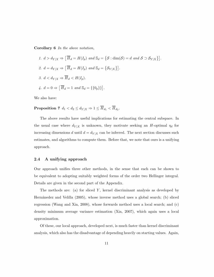
Theorem 5 We have:

1. H(S) ≤ H(Rp) for every subspace S of Rp, equality holding if and only if S is a

dimension reduction subspace (that is, if and only if S ⊇ SY |X).

2. All dimension reduction subspaces contain the same, full, regression information

H(Ip) = H(η), the central subspace being the smallest dimension subspace with

this property.

3. SY |X uniquely maximizes H(·) over all subspaces of dimension dY |X .

The characterization of the central subspace given in the final part of Theorem 5

motivates consideration of the following set of maximization problems, indexed by the

possible values d of dY |X . For each d = 0, 1, ..., p, we define a corresponding set of fixed

matrices Ud, whose members we call d-orthonormal, as follows:

U0 = {0p} and, for d > 0, Ud ={all p × d matrices u with uT u = Id

},

noting that, for d > 0, u1 and u2 in Ud span the same d-dimensional subspace if and

only if u2 = u1Q for some d × d orthogonal matrix Q. Since H is continuous and Ud

compact, there is an ηd maximizing H(·) over Ud, so that Span(ηd) maximizes H(S)

over all subspaces of dimension d. Whereas, for d > 0, ηd is at best unique up to

post-multiplication by an orthogonal matrix, Span(ηd) is unique when d = dY |X (and,

trivially, when d = 0). Putting

Hd = max {H(u) : u ∈ Ud} = max {H(S) : dim(S) = d}

and

Sd ={Span(ηd) : ηd ∈ Ud and H(ηd) = Hd

}

={S : dim(S) = d and H(S) = Hd

},

Proposition 2 and Theorem 5 give at once:

10

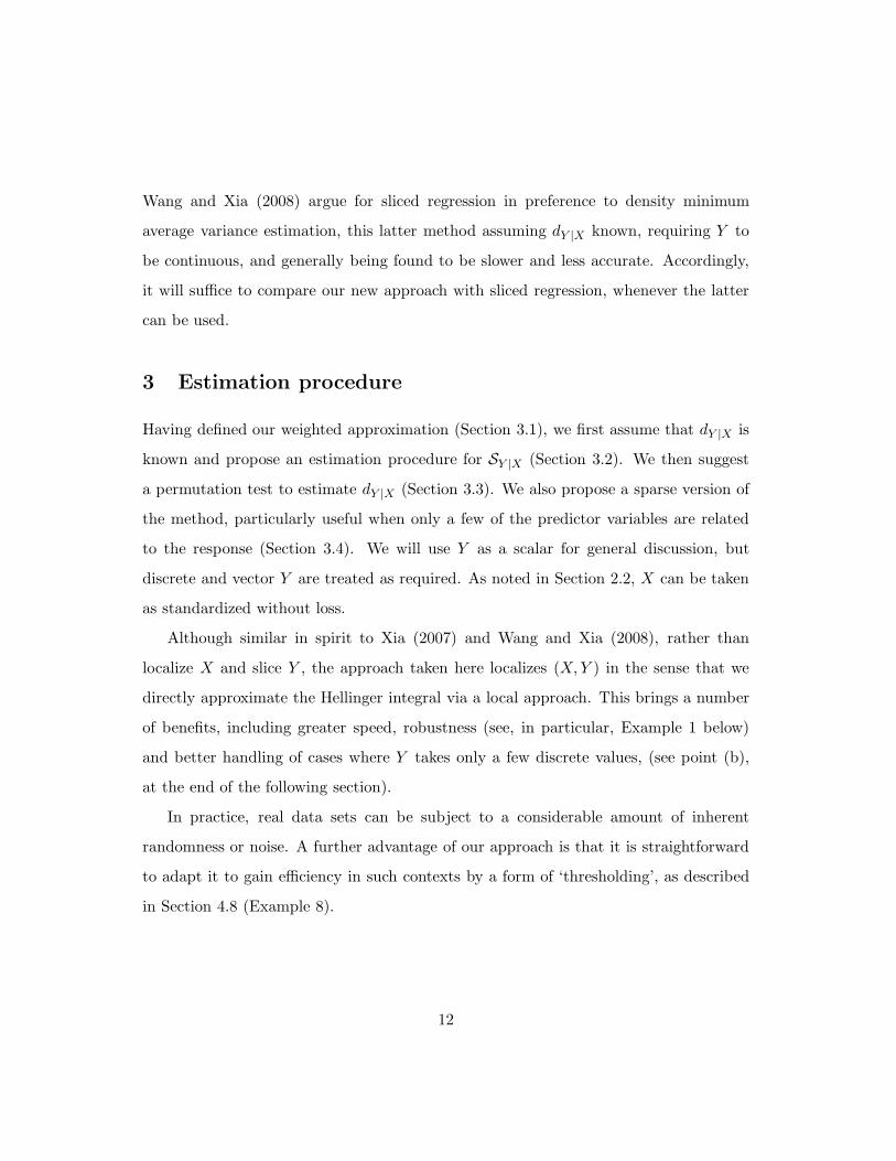
Corollary 6 In the above notation,

1. d > dY |X ⇒[Hd = H(Ip) and Sd =

{S : dim(S) = d and S ⊃ SY |X

}].

2. d = dY |X ⇒[Hd = H(Ip) and Sd =

{SY |X

}].

3. d < dY |X ⇒ Hd < H(Ip).

4. d = 0 ⇒[Hd = 1 and Sd = {{0p}}

].

We also have:

Proposition 7 d1 < d2 ≤ dY |X ⇒ 1 ≤ Hd1< Hd2

.

The above results have useful implications for estimating the central subspace. In

the usual case where dY |X is unknown, they motivate seeking an H-optimal ηd for

increasing dimensions d until d = dY |X can be inferred. The next section discusses such

estimates, and algorithms to compute them. Before that, we note that ours is a unifying

approach.

2.4 A unifying approach

Our approach unifies three other methods, in the sense that each can be shown to

be equivalent to adopting suitably weighted forms of the order two Hellinger integral.

Details are given in the second part of the Appendix.

The methods are: (a) for sliced Y , kernel discriminant analysis as developed by

Hernanedez and Velilla (2005), whose inverse method uses a global search; (b) sliced

regression (Wang and Xia, 2008), whose forwards method uses a local search; and (c)

density minimum average variance estimation (Xia, 2007), which again uses a local

approximation.

Of these, our local approach, developed next, is much faster than kernel discriminant

analysis, which also has the disadvantage of depending heavily on starting values. Again,

11

Wang and Xia (2008) argue for sliced regression in preference to density minimum

average variance estimation, this latter method assuming dY |X known, requiring Y to

be continuous, and generally being found to be slower and less accurate. Accordingly,

it will suffice to compare our new approach with sliced regression, whenever the latter

can be used.

3 Estimation procedure

Having defined our weighted approximation (Section 3.1), we first assume that dY |X is

known and propose an estimation procedure for SY |X (Section 3.2). We then suggest

a permutation test to estimate dY |X (Section 3.3). We also propose a sparse version of

the method, particularly useful when only a few of the predictor variables are related

to the response (Section 3.4). We will use Y as a scalar for general discussion, but

discrete and vector Y are treated as required. As noted in Section 2.2, X can be taken

as standardized without loss.

Although similar in spirit to Xia (2007) and Wang and Xia (2008), rather than

localize X and slice Y , the approach taken here localizes (X,Y ) in the sense that we

directly approximate the Hellinger integral via a local approach. This brings a number

of benefits, including greater speed, robustness (see, in particular, Example 1 below)

and better handling of cases where Y takes only a few discrete values, (see point (b),

at the end of the following section).

In practice, real data sets can be subject to a considerable amount of inherent

randomness or noise. A further advantage of our approach is that it is straightforward

to adapt it to gain efficiency in such contexts by a form of ‘thresholding’, as described

in Section 4.8 (Example 8).

12

3.1 Weighted approximation

To use the Hellinger index, we have to estimate p(x,y)p(x)p(y) . Hence, estimation of p(·)

is critical. For convenience of derivation and without loss of generality, suppose that

dY |X = 1 and consider a particular point (x∗0, y

∗0):

p(x∗0, y

∗0)

p(x∗0)p(y∗0)

=p(ηT x∗

0, y∗0)

p(ηT x∗0)p(y∗0)

.

We put (x0, y0) := (ηT x∗0, y

∗0), denoting a corresponding general point by (x, y). Let

w0(x, y) := 1h1

K(x−x0

h1) 1

h2K(y−y0

h2), where K(.) is a smooth kernel function, symmetric

about 0, h1 and h2 being corresponding bandwidths. Define s2 :=∫

u2K(u)du and

gij :=∫

uivjK(u)K(v)p(x0 − h1u, y0 − h2v)dudv, so that

g00 ∼ p(x0, y0), g10 ∼ −h1s2p10(x0, y0), g01 ∼ −h2s2p

01(x0, y0),

g20 ∼ s2p(x0, y0), g02 ∼ s2p(x0, y0), g11 ∼ h1h2s22p

11(x0, y0),

g22 ∼ s22p(x0, y0), g21 ∼ −h2s

22p

01(x0, y0), g12 ∼ −h1s22p

10(x0, y0),

where pij are the corresponding derivatives for the density. Then,

Ew0(x, y) = p(x0, y0) and

Ew0(x, y)xy =

∫p(x, y)

1

h1K(

x − x0

h1)

1

h2K(

y − y0

h2)xydxdy

=

∫p(x0 − h1u, y0 − h2v)K(u)K(v)(x0 − h1u)(y0 − h2v)dudv

= x0y0g00 − h1y0g10 − x0h2g01 + h1h2g11,

while

Ew0(x, y)x2y2 =

∫p(x, y)

1

h1K(

x − x0

h1)

1

h2K(

y − y0

h2)x2y2dxdy

=

∫p(x0 − h1u, y0 − h2v)K(u)K(v)(x0 − h1u)2(y0 − h2v)2dudv

= x20y

20g00 − 2h1x0y

20g10 + h2

1y20g20 − 2x2

0h2y0g01 + 4h1h2x0y0g11

− 2h2y0h21g21 + x2

0h22g02 − 2h1x0h

22g12 + h2

1h22g22.

13

Similarly, with w0(x) = 1h1

K(x−x0

h1),

Ew0(x) = p(x0) and

Ew0(x)x = x0p(x0) + h21s2p

′(x0),

while

Ew0(x)x2 = x20p(x0) + 2h2

1s2x0p′(x0) + h2

1s2p(x0).

Thus,

p(x0, y0)

p(x0)p(y0)∼ h2

1h22s

22

h21h

22s

22 + h2

1y20s2 + h2

2x20s2

H∗

where

H∗ :=Ew0(x, y)x2y2 − (Ew0(x, y)xy)2/Ew0(x, y)

[Ew0(x)x2 − (Ew0(x)x)2/Ew0(x)][Ew0(y)y2 − (Ew0(y)y)2/Ew0(y)].

Again, without loss of generality, we can assume (x0, y0) = (0, 0) (otherwise, set x′ =

x − x0 and y′ = y − y0, and use the argument with (x′, y′) instead) so that, finally,

p(x∗0, y

∗0)

p(x∗0)p(y∗0)

∼ H∗.

Pooling first, we may find η to maximize∑n

i=1 H∗i , where H∗

i is the H∗ value for the ith

data point. Alternatively, we may maximize H∗i to obtain ηi at each data point, and

then pool the ηi’s together. Here, we adopt the latter approach.

Clearly, the method will depend on the choice of w0. It is interesting to note that,

if all w0(x, y) ≡ 1, η is the dominant eigenvector of V (X)−1V (XY )V (Y )−1, where

V (·) denotes a variance matrix. Suppose that both X and Y are standardized, then

V (X)−1V (XY )V (Y )−1 = E{XXT V (Y |X)}+ V [XE(Y |X)], which may be regarded as

weighted from the regression mean and variance functions. Further, assume that the

linearity and constant variance conditions hold. Then, as an inverse regression,

V (X)−1V (XY )V (Y )−1 = E{Y 2V (X|Y )} + V [Y E(X|Y )]

= E(Y 2)(I − PSY |X) + PSY |X

V (XY )PSY |X

14

which may be simply regarded as the weighted inverse mean and variance functions.

However, the corresponding η may not always be in the central subspace SY |X , under-

lining the importance of the choice of weights.

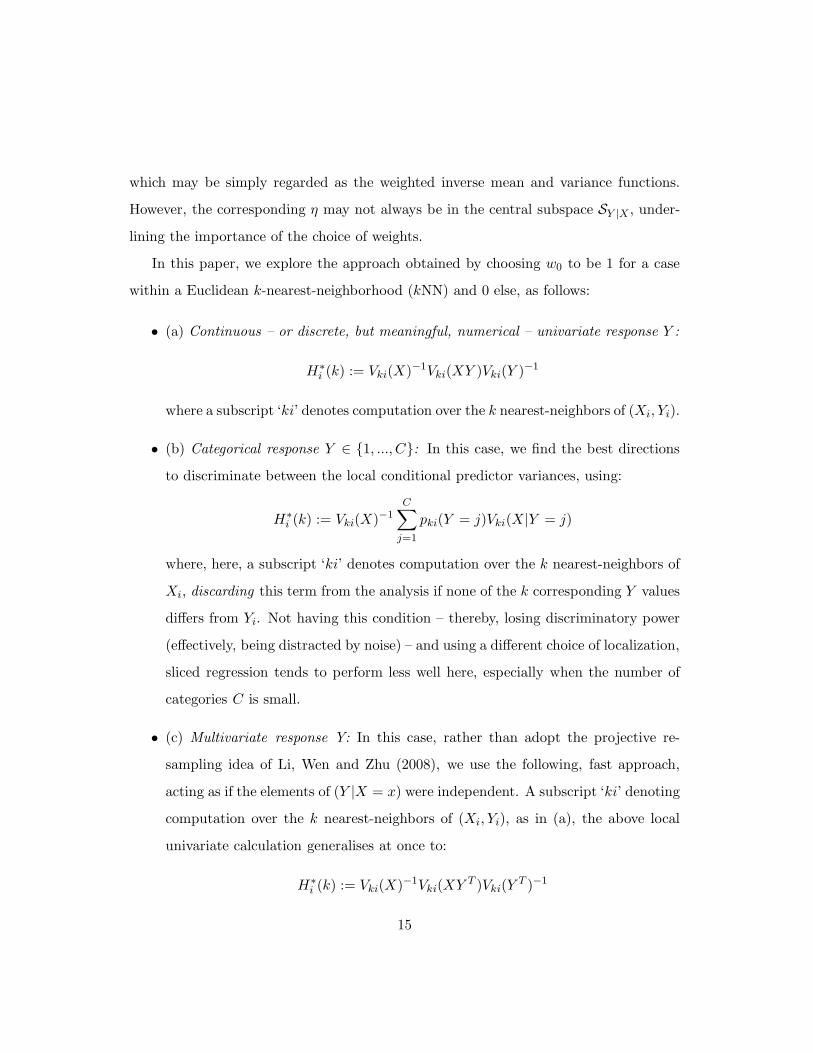
In this paper, we explore the approach obtained by choosing w0 to be 1 for a case

within a Euclidean k-nearest-neighborhood (kNN) and 0 else, as follows:

• (a) Continuous – or discrete, but meaningful, numerical – univariate response Y :

H∗i (k) := Vki(X)−1Vki(XY )Vki(Y )−1

where a subscript ‘ki’ denotes computation over the k nearest-neighbors of (Xi, Yi).

• (b) Categorical response Y ∈ {1, ..., C}: In this case, we find the best directions

to discriminate between the local conditional predictor variances, using:

H∗i (k) := Vki(X)−1

C∑

j=1

pki(Y = j)Vki(X|Y = j)

where, here, a subscript ‘ki’ denotes computation over the k nearest-neighbors of

Xi, discarding this term from the analysis if none of the k corresponding Y values

differs from Yi. Not having this condition – thereby, losing discriminatory power

(effectively, being distracted by noise) – and using a different choice of localization,

sliced regression tends to perform less well here, especially when the number of

categories C is small.

• (c) Multivariate response Y: In this case, rather than adopt the projective re-

sampling idea of Li, Wen and Zhu (2008), we use the following, fast approach,

acting as if the elements of (Y |X = x) were independent. A subscript ‘ki’ denoting

computation over the k nearest-neighbors of (Xi, Yi), as in (a), the above local

univariate calculation generalises at once to:

H∗i (k) := Vki(X)−1Vki(XY T )Vki(Y

T )−1

15

in which the scalar factor involving Vki(YT ) := Eki(Y

T Y ) − Eki(YT )Eki(Y ) is

ignorable as only orthonormal eigenvectors of H∗i (k) are used, as explained in the

following section.

3.2 Algorithm

Assuming dY |X = d is known and that {(xi, yi), i = 1, 2, · · · , n} is an i.i.d. sample

of (X,Y ) values, the algorithm is as follows:

1. For each observation (xi, yi), find its k nearest neighbors in terms of the Euclidean

distance ‖(x, y) − (xi, yi)‖ (‖x − xi‖, if Y is categorical) and, hence, the p × d

orthonormal matrix ηi ≡ (ηi1, ηi2, · · · , ηid) whose columns contain the d dominant

eigenvectors of H∗i (k).

2. Find the spectral decomposition of M := 1nd

∑ni=1 ηiη

Ti , using its dominant d

eigenvectors u := (β1, β2, · · · , βd) to form an estimated basis of SY |X .

The tuning parameter k plays a similar role to the bandwidth in nonparametric

smoothing. Essentially, its choice involves a trade-off between estimation accuracy and

exhaustiveness: for a large enough sample, a larger k can help improve the accuracy

of estimated directions, while a smaller k increases the chance to estimate the central

subspace exhaustively. In this paper, a rough choice of k around 2p seems to work well

across the range of examples presented below. More refined ways to choose k, such as

cross-validation, could of course be used at greater computational expense.

3.3 Determination of the structural dimension dY |X

Recall that dY |X = 0 is equivalent to Y ⊥⊥X. In the population, the orthogonal matrix

of eigenvectors of the kernel dimension reduction matrix, M say, represents a rotation of

the canonical axes of Rp – one for each regressor – to new axes, its eigenvalues reflecting

16

the magnitude of dependence between Y and the corresponding regressors βT X. In

the sample, holding fixed the observed responses y := (y1, ..., yn)T while randomly

permuting the rows of the n × p matrix X := (x1, ..., xn)T will change M , tending to

reduce the magnitude of the corresponding observed dependencies – except, that is,

when dY |X = 0.

Generally, consider testing H0: dY |X = m against Ha: dY |X ≥ (m + 1), for given

m ∈ {0, · · · , p−1}. Sampling variability in (Bm, Am) apart, this is equivalent to testing

Y ⊥⊥ATmX|BT

mX, where Bm := (β1, · · · , βm) and Am := (βm+1, · · · , βp). Accordingly,

the following procedure can be used to determine dY |X :

• Obtain M from the original n×(p+1) data matrix (X,y), computing its spectrum

λ1 > λ2 > · · · > λp and, from it, the test statistic:

f0 = λ(m+1) −1

p − (m + 1)

p∑

i=m+2

λi.

• Apply J independent random permutations to the rows of XAm in the induced

matrix (XBm,XAm,y) to form J permuted data sets, obtaining from each a new

matrix Mj and, hence, a new test statistic fj, (j = 1, · · · , J).

• Compute the permutation p-value:

pperm := J−1J∑

j=1

I(fj > f0),

rejecting H0 if pperm < α.

• Repeat the last two steps for m = 0, 1, . . . until H0 cannot be rejected. Take this

m as the estimated dY |X .

3.4 Sparse version

In some applications, the regression model is held to have an intrinsic sparse structure.

That is, only a few components of X affect the response. In such cases, effectively

17

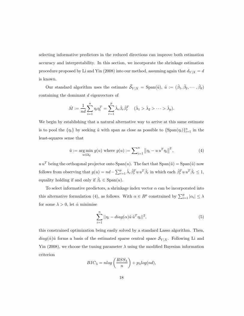
selecting informative predictors in the reduced directions can improve both estimation

accuracy and interpretability. In this section, we incorporate the shrinkage estimation

procedure proposed by Li and Yin (2008) into our method, assuming again that dY |X = d

is known.

Our standard algorithm uses the estimate SY |X = Span(u), u := (β1, β2, · · · , βd)

containing the dominant d eigenvectors of

M :=1

nd

n∑

i=1

ηiηTi =

p∑

r=1

λrβrβTr (λ1 > λ2 > · · · > λp).

We begin by establishing that a natural alternative way to arrive at this same estimate

is to pool the {ηi} by seeking u with span as close as possible to {Span(ηi)}ni=1 in the

least-squares sense that

u := arg minu∈Ud

g(u) where g(u) :=∑n

i=1

∥∥ηi − uuT ηi

∥∥2, (4)

uuT being the orthogonal projector onto Span(u). The fact that Span(u) = Span(u) now

follows from observing that g(u) = nd−∑pr=1 λrβ

Tr uuT βr in which each βT

r uuT βr ≤ 1,

equality holding if and only if βr ∈ Span(u).

To select informative predictors, a shrinkage index vector α can be incorporated into

this alternative formulation (4), as follows. With α ∈ Rp constrained by∑p

i=1 |αi| ≤ λ

for some λ > 0, let α minimise

n∑

i=1

||ηi − diag(α)u uT ηi||2, (5)

this constrained optimization being easily solved by a standard Lasso algorithm. Then,

diag(α)u forms a basis of the estimated sparse central space SY |X . Following Li and

Yin (2008), we choose the tuning parameter λ using the modified Bayesian information

criterion

BICλ = nlog

(RSSλ

n

)+ pλlog(nd),

18

where RSSλ is the residual sum of squares from the fit in (5), pλ being the number of

non-zero elements in α.

4 Evaluation

We evaluate the performance of our method on both simulated and real data.

To measure the accuracy with which Span(u) estimates Span(u), we use each of three

measures proposed in the literature: the vector correlation coefficient, r =∣∣det(uT u)

∣∣

(Ye and Weiss, 2003), the Euclidean distance between projectors, ∆(u, u) =∥∥uuT − uuT

∥∥

(Li, Zha and Chiaromonte, 2005), and the residual length m2 =∥∥(I − uuT )u

∥∥ (Xia et

al, 2002), this last being decomposable by dimension:

m2r =

∥∥(I − uuT )ur

∥∥ where u ≡ (u1, ..., ud).

To measure the effectiveness of variable selection, we use the true positive rate (TPR),

defined as the ratio of the number of predictors correctly identified as active to the

number of active predictors, and the false positive rate (FPR), defined as the ratio of

the number of predictors falsely identified as active to the number of inactive predictors.

All simulation results are based on 100 replications.

To evaluate the effectiveness of our approach, we compare our results with sliced

regression (SR) whenever this method is available, it being reported by Wang and Xia

(2008) to have many advantages (estimation accuracy, exhaustiveness and robustness)

in finite sample performances over many other methods.

4.1 Example 1: A model with frequent extremes

Following Wang and Xia (2008, example 1), Y = (XT β)−1+0.2ǫ, where X = (x1, ..., x10)T

and ǫ i.i.d. standard normal random variables, while β = (1, 1, 1, 1, 0, 0, 0, 0, 0, 0)T , so

that SY |X = span(β). Samples of size n = 200, 400 and 800 are used.

19

Note that extreme Y occurs often in this model, (in particular, for covariate and

error values around their means). Because of this, some existing dimension reduction

methods – such as minimum average variance estimation, sliced inverse regression and

sliced average variance estimation – don’t perform well here, sliced regression standing

out as the best method in Wang and Xia (2008).

Its localization of (X,Y ) filtering the extremes, our method is very robust here.

Applying it to this model, we obtain the results detailed in Table 1.

Table 1: Accuracy of estimates

n r ∆(u, u) m2 CPU time

(in seconds)

200 0.991(0.007) 0.126(0.041) 0.020(0.011) 8

(SR) 0.998(0.001) 0.062(0.022) 0.004(0.002) 265

400 0.996(0.002) 0.079(0.018) 0.007(0.004) 20

(SR) 0.999(0.001) 0.041(0.013) 0.002(0.001) 789

800 0.999(0.001) 0.049(0.012) 0.002(0.001) 57

(SR) 0.999(0.001) 0.026(0.005) 0.001(0.001) 2,519

Overall, estimation accuracy is better for sliced regression, while our method shows

a very significant computational gain. Both the relative accuracy and the relative speed

of our method increase with sample size.

4.2 Example 2: A sparse model

Following Wang and Xia (2008, example 2), who in turn follow Li (1992, model (8.1)),

Y = cos(2X1) − cos(X2) + 0.2ǫ, where X1, ...,X10 and ǫ are i.i.d. standard normal

random variables, so that SY |X = span(e1, e2). Samples of size n = 200, 400 and 800

are used.

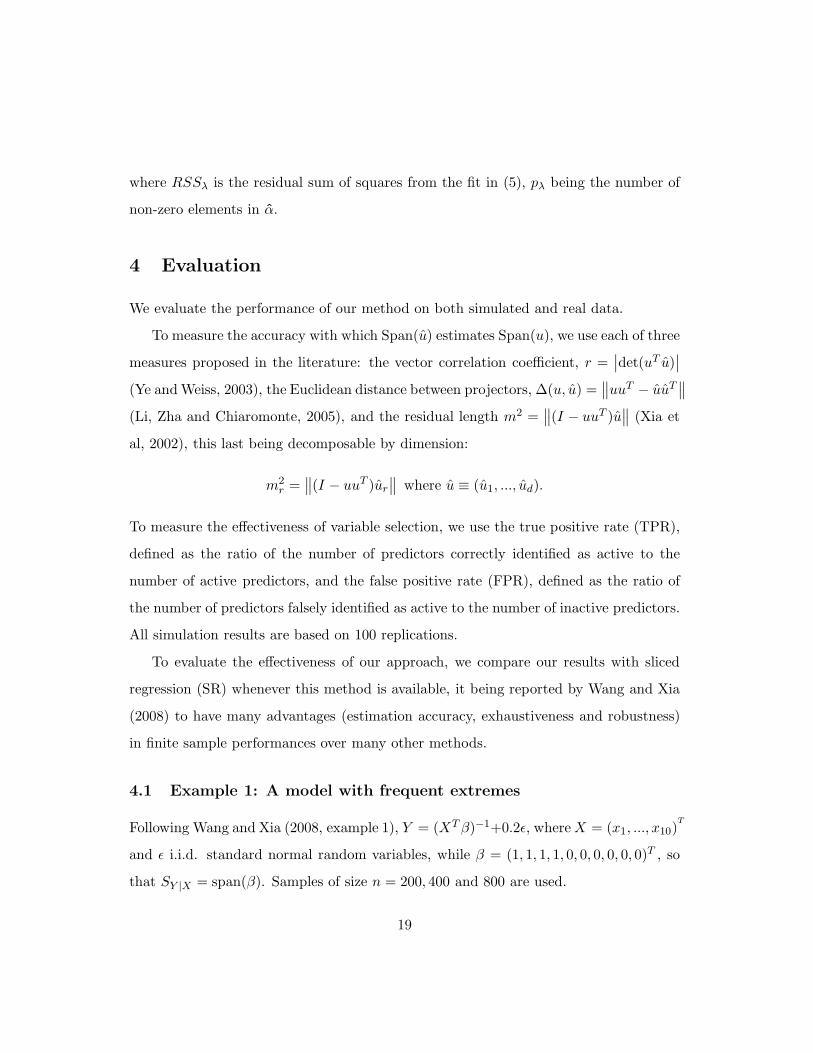
As in the previous example, Table 2 shows that, at very significant computational

cost, the estimation accuracy of sliced regression is greater than for our standard

20

method, whose relative accuracy and speed increase with sample size. Overall, our

sparse method is most accurate, as might be expected. While always good, its TPR

and FPR (reported in Table 3) improve with n.

Table 2: Accuracy of estimates

n r ∆(u, u) m2

1 m2

2 CPU time

(in seconds)

200 0.772(0.162) 0.564(0.178) 0.060(0.031) 0.336(0.213) 8

(Sparse) 0.942(0.183) 0.161(0.231) 0.004(0.012) 0.076(0.198)

(SR) 0.921(0.112) 0.313(0.171) 0.011(0.007) 0.172(0.013) 269

400 0.894(0.105) 0.456(0.151) 0.021(0.010) 0.189(0.137) 20

(Sparse) 0.981(0.081) 0.092(0.146) 0.001(0.002) 0.029(0.103)

(SR) 0.988(0.038) 0.131(0.054) 0.002(0.001) 0.022(0.009) 825

800 0.945(0.029) 0.301(0.078) 0.009(0.005) 0.073(0.044) 58

(Sparse) 0.993(0.014) 0.069(0.093) 0.0004(0.001) 0.013(0.027)

(SR) 0.992(0.010) 0.094(0.023) 0.001(0.001) 0.009(0.005) 2,700

Table 3: Effectiveness of variable selection

Example 2 Example 5

n TPR FPR TPR FPR

200 0.955 0.331 0.938 0.400

400 0.995 0.210 0.974 0.300

800 1.000 0.115 1.000 0.194

4.3 Example 3: A categorical response model

Following Zhu and Zeng (2006), Y = I[Xβ1 + 0.2ǫ > 1] + 2I[Xβ2 + 0.2ǫ > 0], where

X = (x1, ..., x10) and ǫ are i.i.d. standard normal random variables, while β1 =

(1, 1, 1, 1, 0, 0, 0, 0, 0, 0)T

and β2 = (0, 0, 0, 0, 0, 0, 1, 1, 1, 1)T

, so that SY |X = span(β1, β2).

Samples of size n = 200, 400 and 800 are used.

21

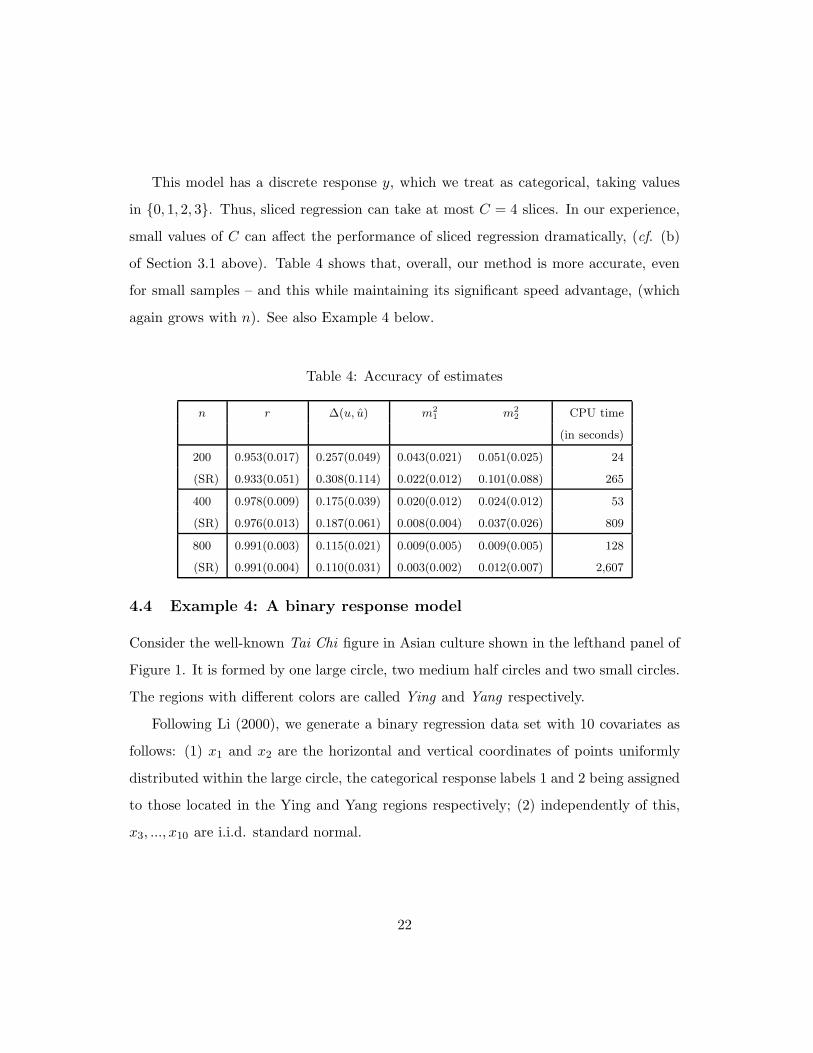
This model has a discrete response y, which we treat as categorical, taking values

in {0, 1, 2, 3}. Thus, sliced regression can take at most C = 4 slices. In our experience,

small values of C can affect the performance of sliced regression dramatically, (cf. (b)

of Section 3.1 above). Table 4 shows that, overall, our method is more accurate, even

for small samples – and this while maintaining its significant speed advantage, (which

again grows with n). See also Example 4 below.

Table 4: Accuracy of estimates

n r ∆(u, u) m2

1 m2

2 CPU time

(in seconds)

200 0.953(0.017) 0.257(0.049) 0.043(0.021) 0.051(0.025) 24

(SR) 0.933(0.051) 0.308(0.114) 0.022(0.012) 0.101(0.088) 265

400 0.978(0.009) 0.175(0.039) 0.020(0.012) 0.024(0.012) 53

(SR) 0.976(0.013) 0.187(0.061) 0.008(0.004) 0.037(0.026) 809

800 0.991(0.003) 0.115(0.021) 0.009(0.005) 0.009(0.005) 128

(SR) 0.991(0.004) 0.110(0.031) 0.003(0.002) 0.012(0.007) 2,607

4.4 Example 4: A binary response model

Consider the well-known Tai Chi figure in Asian culture shown in the lefthand panel of

Figure 1. It is formed by one large circle, two medium half circles and two small circles.

The regions with different colors are called Ying and Yang respectively.

Following Li (2000), we generate a binary regression data set with 10 covariates as

follows: (1) x1 and x2 are the horizontal and vertical coordinates of points uniformly

distributed within the large circle, the categorical response labels 1 and 2 being assigned

to those located in the Ying and Yang regions respectively; (2) independently of this,

x3, ..., x10 are i.i.d. standard normal.

22

(a) Tai Chi (b) Projection onto x1 and x2

Figure 1: Tai Chi figure

Table 5: Accuracy of estimates: Tai Chi data

n r ∆(u, u) m2

1 m2

2

200 0.995(0.003) 0.084(0.023) 0.006(0.004) 0.004(0.003)

(SR) 0.409(0.231) 0.965(0.142) 0.714(0.206) 0.023(0.011)

400 0.998(0.001) 0.056(0.014) 0.003(0.002) 0.002(0.001)

(SR) 0.440(0.269) 0.837(0.174) 0.713(0.254) 0.009(0.005)

800 0.999(0.0003) 0.037(0.007) 0.001(0.001) 0.001(0.001)

(SR) 0.514(0.305) 0.766(0.234) 0.633(0.306) 0.004(0.002)

Li (2000) analyzed this example from the perspective of dimension reduction. Due to

the binary response, sliced inverse regression can only find 1 direction and so he proposed

a double slicing scheme to identify the second direction. Here, we apply our method and

sliced regression to these data. Both our permutation test and cross-validation indicate

a structural dimension of two. Table 5 shows that our much faster method is also much

more accurate here, sliced regression effectively missing the second direction (reasons for

its relatively poor performance in contexts such as this having been discussed above).

23

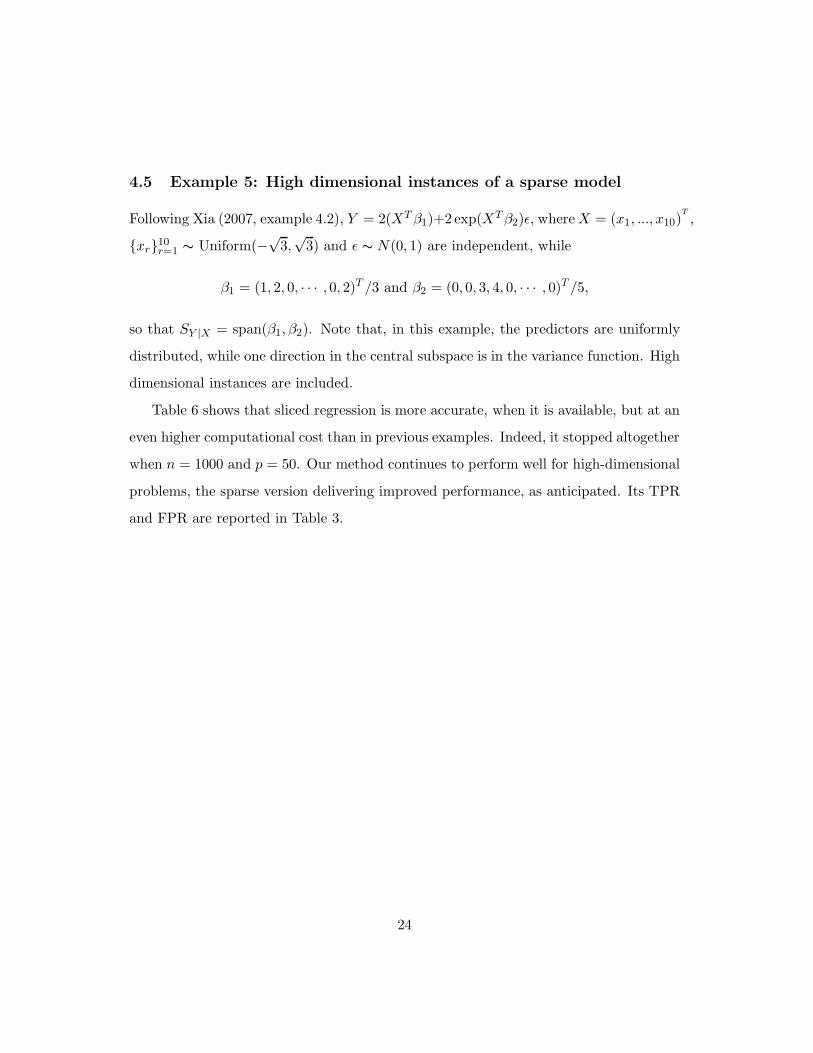
4.5 Example 5: High dimensional instances of a sparse model

Following Xia (2007, example 4.2), Y = 2(XT β1)+2 exp(XT β2)ǫ, where X = (x1, ..., x10)T

,

{xr}10r=1 ∼ Uniform(−

√3,√

3) and ǫ ∼ N(0, 1) are independent, while

β1 = (1, 2, 0, · · · , 0, 2)T /3 and β2 = (0, 0, 3, 4, 0, · · · , 0)T /5,

so that SY |X = span(β1, β2). Note that, in this example, the predictors are uniformly

distributed, while one direction in the central subspace is in the variance function. High

dimensional instances are included.

Table 6 shows that sliced regression is more accurate, when it is available, but at an

even higher computational cost than in previous examples. Indeed, it stopped altogether

when n = 1000 and p = 50. Our method continues to perform well for high-dimensional

problems, the sparse version delivering improved performance, as anticipated. Its TPR

and FPR are reported in Table 3.

24

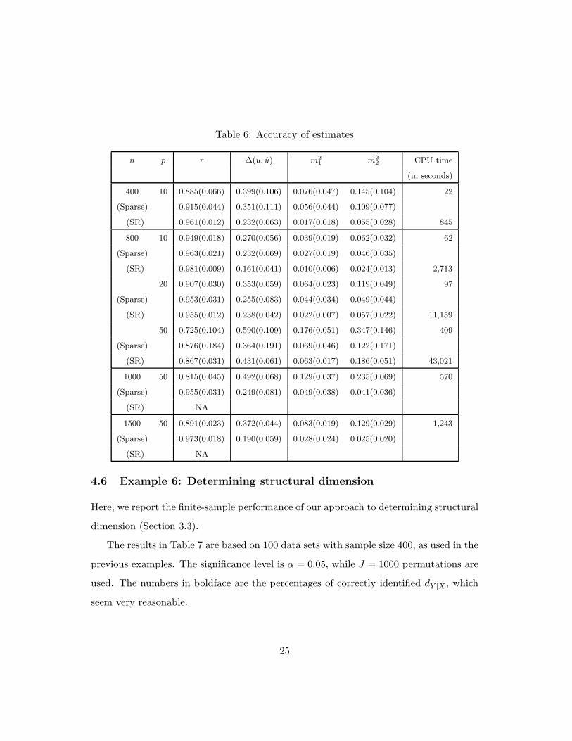
Table 6: Accuracy of estimates

n p r ∆(u, u) m2

1 m2

2 CPU time

(in seconds)

400 10 0.885(0.066) 0.399(0.106) 0.076(0.047) 0.145(0.104) 22

(Sparse) 0.915(0.044) 0.351(0.111) 0.056(0.044) 0.109(0.077)

(SR) 0.961(0.012) 0.232(0.063) 0.017(0.018) 0.055(0.028) 845

800 10 0.949(0.018) 0.270(0.056) 0.039(0.019) 0.062(0.032) 62

(Sparse) 0.963(0.021) 0.232(0.069) 0.027(0.019) 0.046(0.035)

(SR) 0.981(0.009) 0.161(0.041) 0.010(0.006) 0.024(0.013) 2,713

20 0.907(0.030) 0.353(0.059) 0.064(0.023) 0.119(0.049) 97

(Sparse) 0.953(0.031) 0.255(0.083) 0.044(0.034) 0.049(0.044)

(SR) 0.955(0.012) 0.238(0.042) 0.022(0.007) 0.057(0.022) 11,159

50 0.725(0.104) 0.590(0.109) 0.176(0.051) 0.347(0.146) 409

(Sparse) 0.876(0.184) 0.364(0.191) 0.069(0.046) 0.122(0.171)

(SR) 0.867(0.031) 0.431(0.061) 0.063(0.017) 0.186(0.051) 43,021

1000 50 0.815(0.045) 0.492(0.068) 0.129(0.037) 0.235(0.069) 570

(Sparse) 0.955(0.031) 0.249(0.081) 0.049(0.038) 0.041(0.036)

(SR) NA

1500 50 0.891(0.023) 0.372(0.044) 0.083(0.019) 0.129(0.029) 1,243

(Sparse) 0.973(0.018) 0.190(0.059) 0.028(0.024) 0.025(0.020)

(SR) NA

4.6 Example 6: Determining structural dimension

Here, we report the finite-sample performance of our approach to determining structural

dimension (Section 3.3).

The results in Table 7 are based on 100 data sets with sample size 400, as used in the

previous examples. The significance level is α = 0.05, while J = 1000 permutations are

used. The numbers in boldface are the percentages of correctly identified dY |X , which

seem very reasonable.

25

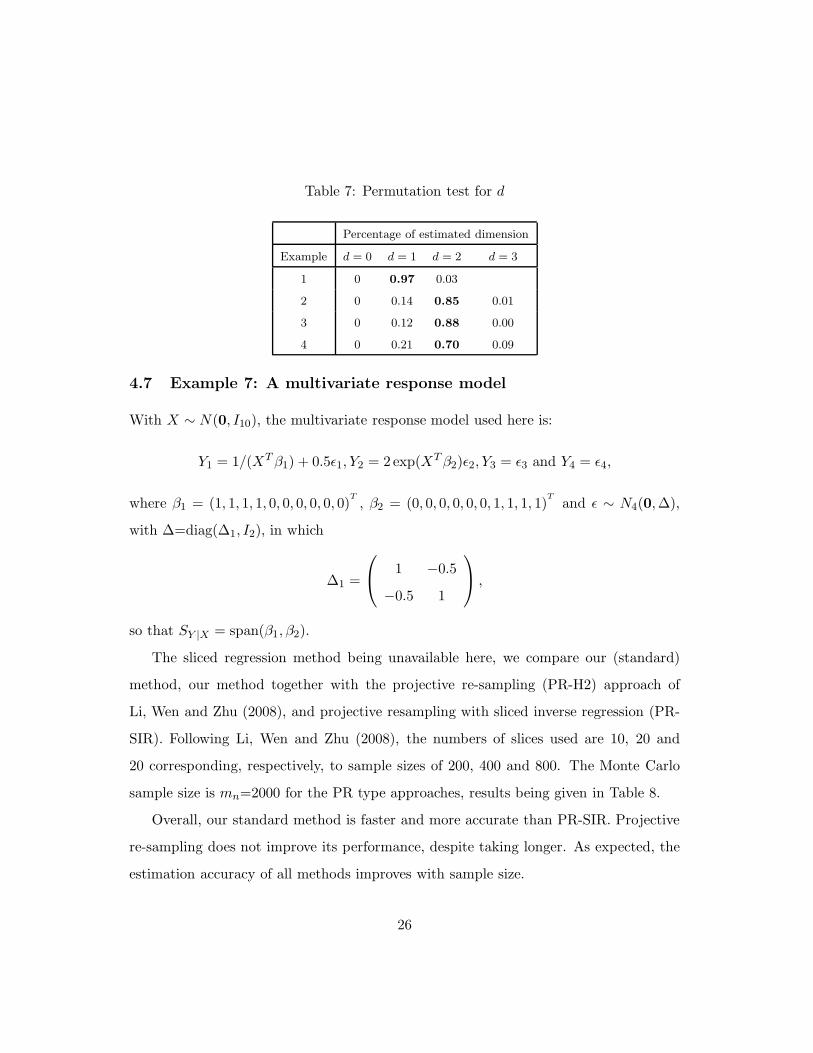
Table 7: Permutation test for d

Percentage of estimated dimension

Example d = 0 d = 1 d = 2 d = 3

1 0 0.97 0.03

2 0 0.14 0.85 0.01

3 0 0.12 0.88 0.00

4 0 0.21 0.70 0.09

4.7 Example 7: A multivariate response model

With X ∼ N(0, I10), the multivariate response model used here is:

Y1 = 1/(XT β1) + 0.5ǫ1, Y2 = 2exp(XT β2)ǫ2, Y3 = ǫ3 and Y4 = ǫ4,

where β1 = (1, 1, 1, 1, 0, 0, 0, 0, 0, 0)T

, β2 = (0, 0, 0, 0, 0, 0, 1, 1, 1, 1)T

and ǫ ∼ N4(0,∆),

with ∆=diag(∆1, I2), in which

∆1 =

1 −0.5

−0.5 1

,

so that SY |X = span(β1, β2).

The sliced regression method being unavailable here, we compare our (standard)

method, our method together with the projective re-sampling (PR-H2) approach of

Li, Wen and Zhu (2008), and projective resampling with sliced inverse regression (PR-

SIR). Following Li, Wen and Zhu (2008), the numbers of slices used are 10, 20 and

20 corresponding, respectively, to sample sizes of 200, 400 and 800. The Monte Carlo

sample size is mn=2000 for the PR type approaches, results being given in Table 8.

Overall, our standard method is faster and more accurate than PR-SIR. Projective

re-sampling does not improve its performance, despite taking longer. As expected, the

estimation accuracy of all methods improves with sample size.

26

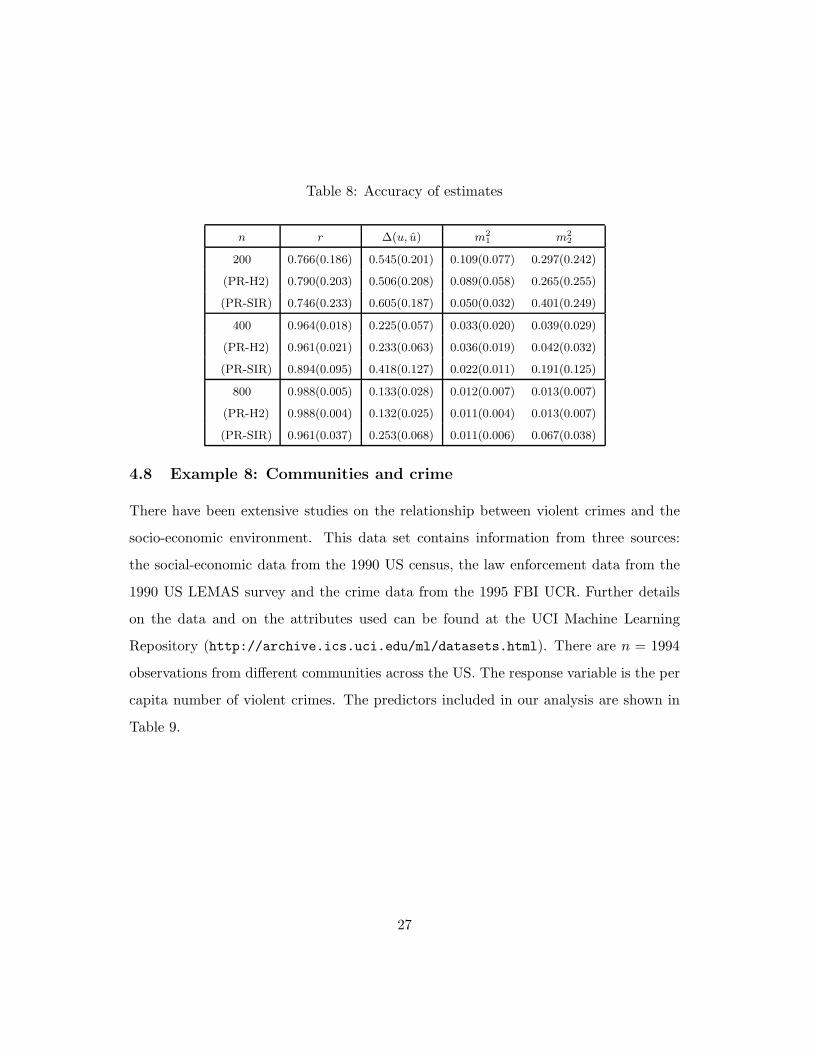
Table 8: Accuracy of estimates

n r ∆(u, u) m2

1 m2

2

200 0.766(0.186) 0.545(0.201) 0.109(0.077) 0.297(0.242)

(PR-H2) 0.790(0.203) 0.506(0.208) 0.089(0.058) 0.265(0.255)

(PR-SIR) 0.746(0.233) 0.605(0.187) 0.050(0.032) 0.401(0.249)

400 0.964(0.018) 0.225(0.057) 0.033(0.020) 0.039(0.029)

(PR-H2) 0.961(0.021) 0.233(0.063) 0.036(0.019) 0.042(0.032)

(PR-SIR) 0.894(0.095) 0.418(0.127) 0.022(0.011) 0.191(0.125)

800 0.988(0.005) 0.133(0.028) 0.012(0.007) 0.013(0.007)

(PR-H2) 0.988(0.004) 0.132(0.025) 0.011(0.004) 0.013(0.007)

(PR-SIR) 0.961(0.037) 0.253(0.068) 0.011(0.006) 0.067(0.038)

4.8 Example 8: Communities and crime

There have been extensive studies on the relationship between violent crimes and the

socio-economic environment. This data set contains information from three sources:

the social-economic data from the 1990 US census, the law enforcement data from the

1990 US LEMAS survey and the crime data from the 1995 FBI UCR. Further details

on the data and on the attributes used can be found at the UCI Machine Learning

Repository (http://archive.ics.uci.edu/ml/datasets.html). There are n = 1994

observations from different communities across the US. The response variable is the per

capita number of violent crimes. The predictors included in our analysis are shown in

Table 9.

27

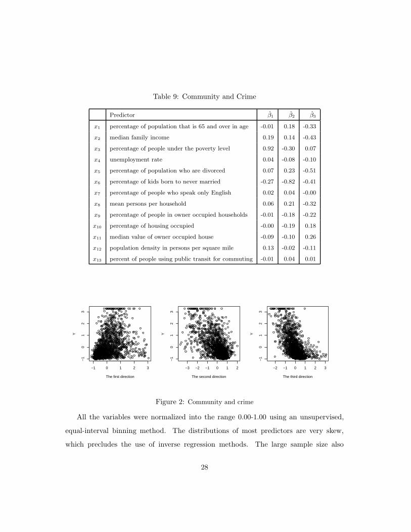
Table 9: Community and Crime

Predictor β1 β2 β3

x1 percentage of population that is 65 and over in age -0.01 0.18 -0.33

x2 median family income 0.19 0.14 -0.43

x3 percentage of people under the poverty level 0.92 -0.30 0.07

x4 unemployment rate 0.04 -0.08 -0.10

x5 percentage of population who are divorced 0.07 0.23 -0.51

x6 percentage of kids born to never married -0.27 -0.82 -0.41

x7 percentage of people who speak only English 0.02 0.04 -0.00

x8 mean persons per household 0.06 0.21 -0.32

x9 percentage of people in owner occupied households -0.01 -0.18 -0.22

x10 percentage of housing occupied -0.00 -0.19 0.18

x11 median value of owner occupied house -0.09 -0.10 0.26

x12 population density in persons per square mile 0.13 -0.02 -0.11

x13 percent of people using public transit for commuting -0.01 0.04 0.01

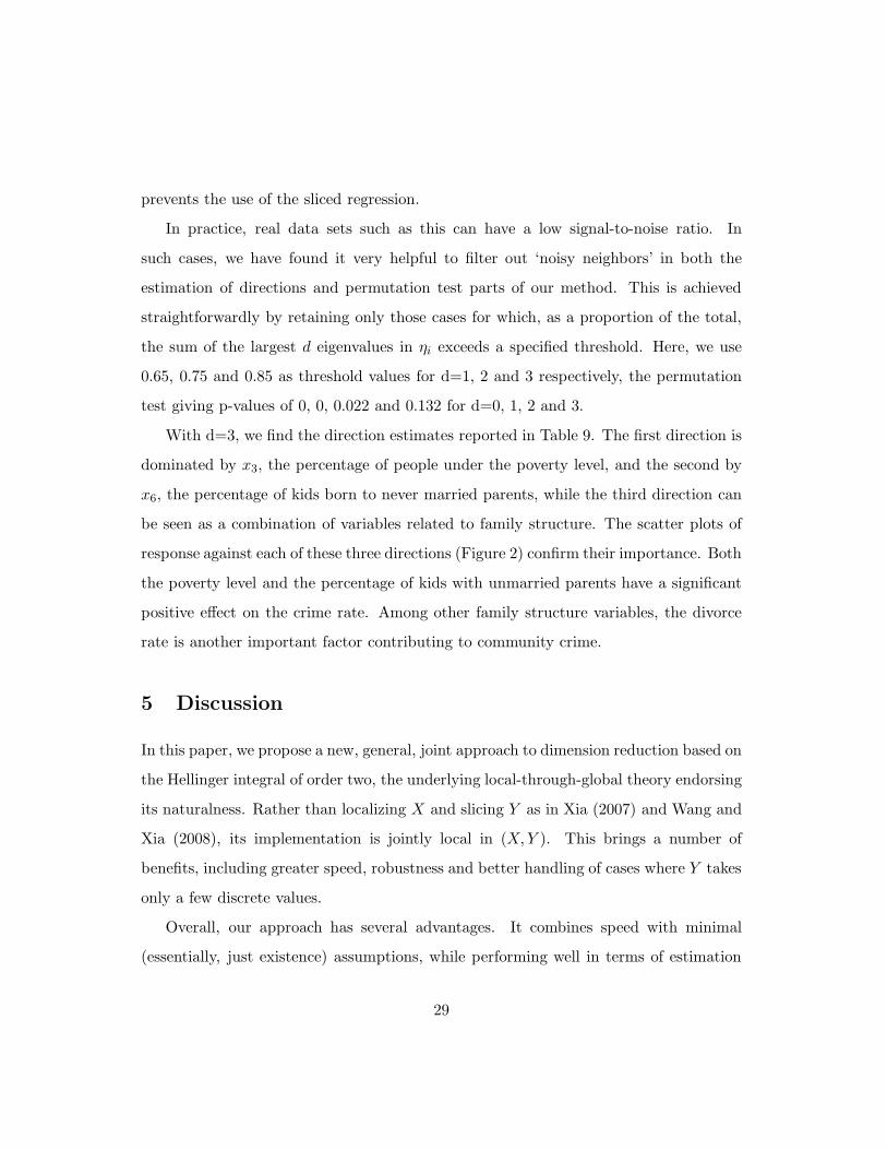
−1 0 1 2 3

−1

01

23

The first direction

Y

−3 −2 −1 0 1 2

−1

01

23

The second direction

Y

−2 −1 0 1 2 3

−1

01

23

The third direction

Y

Figure 2: Community and crime

All the variables were normalized into the range 0.00-1.00 using an unsupervised,

equal-interval binning method. The distributions of most predictors are very skew,

which precludes the use of inverse regression methods. The large sample size also

28

prevents the use of the sliced regression.

In practice, real data sets such as this can have a low signal-to-noise ratio. In

such cases, we have found it very helpful to filter out ‘noisy neighbors’ in both the

estimation of directions and permutation test parts of our method. This is achieved

straightforwardly by retaining only those cases for which, as a proportion of the total,

the sum of the largest d eigenvalues in ηi exceeds a specified threshold. Here, we use

0.65, 0.75 and 0.85 as threshold values for d=1, 2 and 3 respectively, the permutation

test giving p-values of 0, 0, 0.022 and 0.132 for d=0, 1, 2 and 3.

With d=3, we find the direction estimates reported in Table 9. The first direction is

dominated by x3, the percentage of people under the poverty level, and the second by

x6, the percentage of kids born to never married parents, while the third direction can

be seen as a combination of variables related to family structure. The scatter plots of

response against each of these three directions (Figure 2) confirm their importance. Both

the poverty level and the percentage of kids with unmarried parents have a significant

positive effect on the crime rate. Among other family structure variables, the divorce

rate is another important factor contributing to community crime.

5 Discussion

In this paper, we propose a new, general, joint approach to dimension reduction based on

the Hellinger integral of order two, the underlying local-through-global theory endorsing

its naturalness. Rather than localizing X and slicing Y as in Xia (2007) and Wang and

Xia (2008), its implementation is jointly local in (X,Y ). This brings a number of

benefits, including greater speed, robustness and better handling of cases where Y takes

only a few discrete values.

Overall, our approach has several advantages. It combines speed with minimal

(essentially, just existence) assumptions, while performing well in terms of estimation

29

accuracy, robustness and exhaustiveness, this last due to its local weight approximation.

Relative to sliced regression (Wang and Xia, 2008), examples show that our approach:

(a) is significantly faster without losing too much estimation accuracy, allowing larger

problems to be tackled, (b) is more general, multidimensional (discrete, continuous or

mixed) Y as well as X being allowed, and (c) benefits from having a sparse version,

this enabling variable selection while making overall performance broadly comparable.

Finally, incorporating appropriate weights, it unifies three existing methods, including

sliced regression.

Among other further work, a global search of the Hellinger integral with or without

slicing, similar to that of Hernanedez and Velilla (2005), merits investigation. That said,

being based on nonparametric density estimation, this may turn out to be slow, depend

heavily on starting values, or be less accurate than a local approach, in particular when

dY |X > 1.

6 Appendix: Additional materials

In this section, we provide additional materials. First part is the proof of the Theoretical

results. Second part is the links to some existing methods.

6.1 Additional justifications

We provide here justifications of results not given in the body of the paper.

Proposition 1

It suffices to show the first implication. Now, Span(u1) = Span(u2) ⇒ rank(u1) =

rank(u2) = r, say. Suppose first that r = 0. Then, for i = 1, 2, ui vanishes, so that

Y ⊥⊥uTi X implying R(y;uT

i x)(y,x)≡ 1. Otherwise, let u be any matrix whose 1 ≤ r ≤ p

columns form a basis for Span(u1) = Span(u2). Then, for i = 1, 2, ui = uATi for some

30

Ai of full column rank, so that

uT1 X = uT

1 x ⇔ uT X = uT x ⇔ uT2 X = uT

2 x.

Thus, p(y|uT1 x)

(y,x)≡ p(y|uT

2 x) implying R(y;uT1 x)

(y,x)≡ R(y;uT

2 x).

Theorem 5

Since the central subspace is the intersection of all dimension reduction subspaces,

it suffices to prove (1). If S = Rp, the result is trivial. Again, if S = {0p}, it follows

at once from Proposition 3. Otherwise, it follows from Proposition 4, taking S2 as the

orthogonal complement in Rp of S1 = S.

Proposition 7

The inequality 1 ≤ Hd1is immediate from Propositions 2 and 3. The proof that

Hd1< Hd2

is by contradiction. Consider first the case d1 > 0 and, for a given ηd1, let

u be any matrix such that (ηd1, u) ∈ Ud2

. Then,

Hd2− Hd1

≥ H(ηd1, u) − H(ηd1

) ≥ 0,

the second inequality here using Proposition 4. Suppose, if possible, that Hd1= Hd2

.

Then, H(ηd1, u) = H(ηd1

) for any such u so that, using Proposition 4, Y ⊥⊥ vT X|ηTd1

X

for any vector v. It follows that Span(ηd1) is a dimension reduction subspace, contrary

to d1 < dY |X . The proof when d1 = 0 is entirely similar, using Proposition 3.

6.2 Unification of three existing methods

Kernel Discriminant Analysis (Hernanedez and Velilla, 2005)

Suppose that Y is a discrete response where, for some countable index set Y ⊂ R,

Y = y with probability p(y) > 0(∑

y∈Y p(y) = 1)

and, we assume, for each y ∈ Y, X

31

admits a conditional density p(x|y) so that

p(x) =∑

y∈Y

p(y, x) where p(y, x) = p(y)p(x|y) = p(x)p(y|x),

whence

p(uT x) =∑

y∈Y

p(y, uT x) where p(y, uT x) = p(y)p(uT x|y) = p(uT x)p(y|uT x). (6)

In the discrete case, it is natural to use the following form of H(·) as our basis for

estimation:

H(u) = E

(p(uT X|Y )

p(uT X)

).

For example, in the binary case, by (6), we need just two m-dimensional estimates:

p(uT x|Y = 0) and p(uT x|Y = 1)

obtained from (kernel) smoothing the corresponding partition of the data.

Thus,

H(u) = EY EuT X|Y

(p(uT X|Y )

p(uT X)

)

=∑

y∈Y

p(y)

∫ (p2(uT x|y)

p(uT x)

).

Hernanedez and Velilla (2005) proposed a method which maximises the following

index:

IHV (u) :=∑

y∈Y

varuT X

(p(y)

p(uT x|y)

p(uT x)

).

Since

IHV (u) =∑

y∈Y

p2(y)varuT X

(p(uT x|y)

p(uT x)

)

=∑

y∈Y

p2(y)

∫ (p2(uT x|y)

p(uT x)

)− a

32

where a :=∑

y∈Y p2(y) is constant, their index is equivalent to ours, except that the

weight function p(y) is squared.

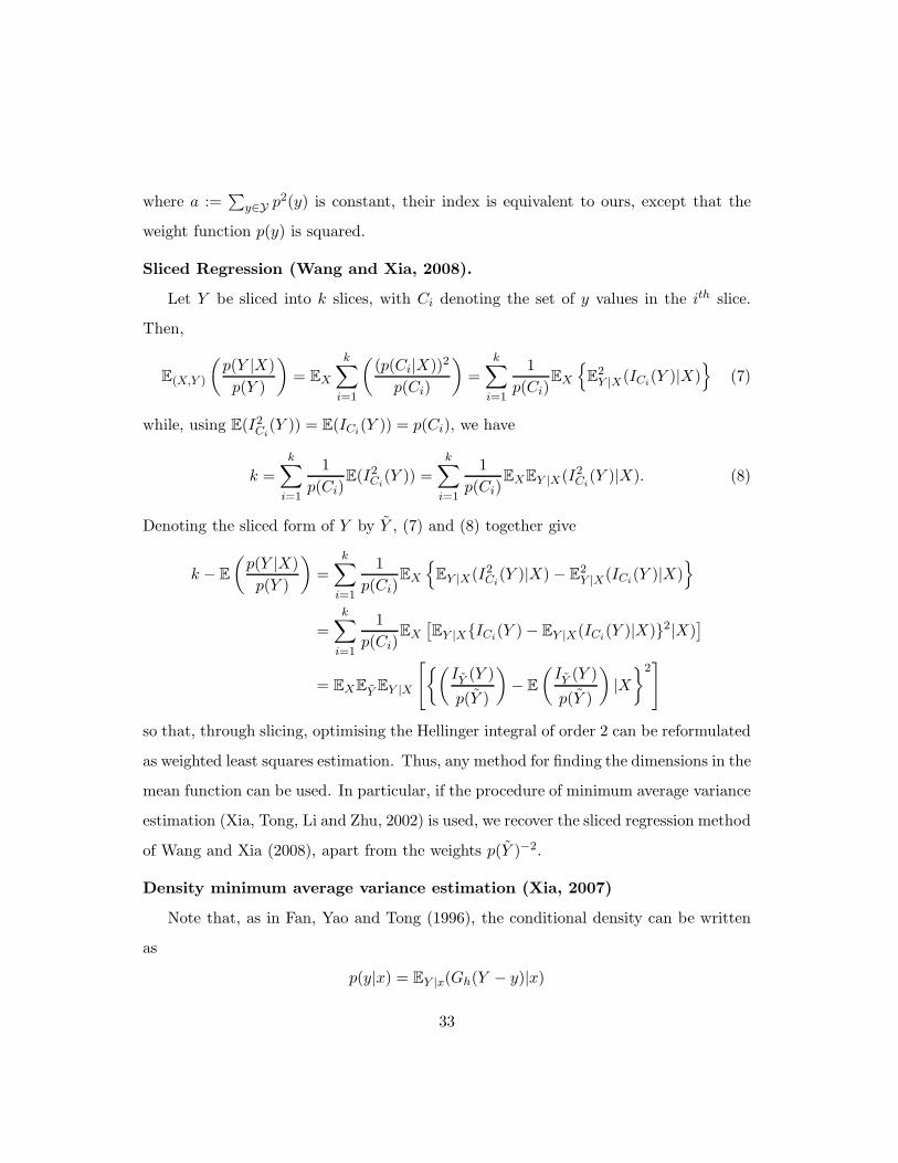
Sliced Regression (Wang and Xia, 2008).

Let Y be sliced into k slices, with Ci denoting the set of y values in the ith slice.

Then,

E(X,Y )

(p(Y |X)

p(Y )

)= EX

k∑

i=1

((p(Ci|X))2

p(Ci)

)=

k∑

i=1

1

p(Ci)EX

{E

2Y |X(ICi

(Y )|X)}

(7)

while, using E(I2Ci

(Y )) = E(ICi(Y )) = p(Ci), we have

k =

k∑

i=1

1

p(Ci)E(I2

Ci(Y )) =

k∑

i=1

1

p(Ci)EXEY |X(I2

Ci(Y )|X). (8)

Denoting the sliced form of Y by Y , (7) and (8) together give

k − E

(p(Y |X)

p(Y )

)=

k∑

i=1

1

p(Ci)EX

{EY |X(I2

Ci(Y )|X) − E

2Y |X(ICi

(Y )|X)}

=k∑

i=1

1

p(Ci)EX

[EY |X{ICi

(Y ) − EY |X(ICi(Y )|X)}2|X)

]

= EXEY EY |X

[{(IY (Y )

p(Y )

)− E

(IY (Y )

p(Y )

)|X

}2]

so that, through slicing, optimising the Hellinger integral of order 2 can be reformulated

as weighted least squares estimation. Thus, any method for finding the dimensions in the

mean function can be used. In particular, if the procedure of minimum average variance

estimation (Xia, Tong, Li and Zhu, 2002) is used, we recover the sliced regression method

of Wang and Xia (2008), apart from the weights p(Y )−2.

Density minimum average variance estimation (Xia, 2007)

Note that, as in Fan, Yao and Tong (1996), the conditional density can be written

as

p(y|x) = EY |x(Gh(Y − y)|x)

33

where G is a kernel and h is the bandwidth, so that

E

(p(Y |X)

p(Y )

)=

∫p(x)

p(y)E

2Y |x(Gh(Y − y)|x)dxdy.

Thus, defining the constant

a0 :=

∫p(x)

p(y)EY |xG

2h(Y − y)dxdy,

we have

a0 − E

(p(Y |X)

p(Y )

)=

∫p(x)

p(y)E {Gh(Y − y) − E(Gh(Y − y)|x)}2 dxdy

=

∫p(x)p(y)E

{Gh(Y − y)

p(y)− E

(Gh(Y − y)

p(y)|x

)}2

dxdy

= ExEyEY |x

{Gh(Y − y)

p(y)− E

(Gh(Y − y)

p(y)|x

)}2

Therefore, density minimum average variance estimation and density outer product of

gradient (Xia, 2007) are methods to estimate the last term, apart from the weight

p(y)−2.

References

Bura, E. and Cook, R. D. (2001). Estimating the structural dimension of regressions

via parametric inverse regression. Journal of the Royal Statistical Society B, 63,

393–410.

Cook, R. D. (1998a). Principal Hessian directions revisited (with discussion). Journal

of the American Statistical Association, 93, 84–100.

Cook, R. D. (1998b). Regression Graphics: Ideas for studying regressions through

graphics. New York: Wiley.

34

Cook, R. D. and Ni, L. (2005). Sufficient dimension reduction via inverse regression: a

minimum discrepancy approach. Journal of the American Statistical Association,

100, 410–428.

Cook, R. D. and Weisberg, S. (1991). Discussion of Li (1991), Journal of the American

Statistical Association, 86, 328–332.

Fan, J., Yao, Q. and Tong, H. (1996). Estimation of conditional densities and sensi-

tivity measures in nonlinear dynamical systems. Biometrika, 83, 189-196.

Hardle, W. and Stoker, T. M. (1989). Investigating smooth multiple regression by

method of average derivatives. Journal of the American Statistical Association,

84, 986–995.

Hernandez, A. and Velilla, S. (2005). Dimension reduction in nonparametric kernel

discriminant analysis, Journal of Computational & Graphical Statistics, 14, 847–

866.

Hristache, M., Juditsky, A., Polzehl, J. and Spokoiny, V. (2001). Structure adaptive

approach to dimension reduction. The Annals of Statistics, 29, 1537–1566.

Li, B., Zha, H. and Chiaromonte, F. (2005). Contour regression: a general approach

to dimension reduction. The Annals of Statistics, 33, 1580–1616.

Li, B., Wen, S. and Zhu, L. (2008). On a projective resampling method for dimen-

sion reduction with multivariate responses. Journal of the American Statistical

Association, 103, 1177–1186.

Li, K. C. (1991). Sliced inverse regression for dimension reduction (with discussion).

Journal of the American Statistical Association, 86, 316–342.

35

Li, K. C. (1992). On principal Hessian directions for data visualization and dimen-

sion reduction: Another application of Stein’s lemma. Journal of the American

Statistical Association, 87, 1025–1039.

Li, K. C. (2000). High dimensional data analysis via the SIR/PHD approach. Lecture

Notes obtained from http://www.stat.ucla.edu/~kcli/sir-PHD.pdf

Li, L. and Yin, X. (2008). Sliced inverse regression with regularizations. Biometrics,

64, 124-131.

Samarov, A. M. (1993). Exploring regression structure using nonparametric function

estimation. Journal of the American Statistical Association, 88, 836–847.

Wang, H. and Xia, Y. (2008). Sliced Regression for Dimension Reduction. Journal of

the American Statistical Association, 103, 811–821.

Xia, Y. (2007). A constructive approach to the estimation of dimension reduction

directions. The Annals of Statistics, 35, 2654–2690.

Xia, Y., Tong, H., Li, W. and Zhu, L. (2002). An adaptive estimation of dimension

reduction space. Journal of the Royal Statistical Society B, 64, 363–410.

Ye, Z. and Weiss, R. E. (2003). Using the bootstrap to select one of a new class of

dimension reduction methods. Journal of the American Statistical Association,

98, 968–979.

Yin, X. and Cook, R. D. (2002). Dimension reduction for the conditional k-th moment

in regression. Journal of the Royal Statistical Society B, 64, 159–175.

Yin, X. and Cook, R. D. (2003). Estimating central subspaces via inverse third mo-

ments. Biometrika, 90, 113-125.

36

Yin, X. and Cook, R. D. (2005). Direction estimation in single-index regressions.

Biometrika, 92, 371-384.

Yin, X., Li, B. and Cook, R. D. (2008). Successive direction extraction for estimat-

ing the central subspace in a Multiple-index regression. Journal of Multivariate

Analysis, 99, 1733–1757.

Zhu, Y. and Zeng, P. (2006). Fourier methods for estimating the central subspace

and the central mean subspace in regression. Journal of the American Statistical

Association, 101, 1638–1651.

37