Succinct Hitting Sets and Barriers to Proving AlgebraicCircuits Lower Bounds

Michael A. Forbes∗ Amir Shpilka† Ben Lee Volk†

Abstract

We formalize a framework of algebraically natural lower bounds for algebraic circuits. Justas with the natural proofs notion of Razborov and Rudich [RR97] for boolean circuit lowerbounds, our notion of algebraically natural lower bounds captures nearly all lower boundtechniques known. However, unlike the boolean setting, there has been no concrete evidencedemonstrating that this is a barrier to obtaining super-polynomial lower bounds for generalalgebraic circuits, as there is little understanding whether algebraic circuits are expressiveenough to support “cryptography” secure against algebraic circuits.

Following a similar result of Williams [Wil16] in the boolean setting, we show that theexistence of an algebraic natural proofs barrier is equivalent to the existence of succinct deran-domization of the polynomial identity testing problem. That is, whether the coefficient vec-tors of polylog(N)-degree polylog(N)-size circuits is a hitting set for the class of poly(N)-degreepoly(N)-size circuits. Further, we give an explicit universal construction showing that if sucha succinct hitting set exists, then our universal construction suffices.

Further, we assess the existing literature constructing hitting sets for restricted classes ofalgebraic circuits and observe that none of them are succinct as given. Yet, we show how tomodify some of these constructions to obtain succinct hitting sets. This constitutes the firstevidence supporting the existence of an algebraic natural proofs barrier.

Our framework is similar to the Geometric Complexity Theory (GCT) program of Mulmu-ley and Sohoni [MS01], except that here we emphasize constructiveness of the proofs while theGCT program emphasizes symmetry. Nevertheless, our succinct hitting sets have relevance tothe GCT program as they imply lower bounds for the complexity of the defining equations ofpolynomials computed by small circuits.

∗University of Illinois at Urbana-Champaign. E-mail: miforbes@illinois.edu. This work was performed when theauthor was at Stanford University, while supported by the NSF, including NSF CCF-1617580, and the DARPA Safewareprogram.†Department of Computer Science, Tel Aviv University, Tel Aviv, Israel, E-mails: shpilka@post.tau.ac.il,

benleevolk@gmail.com. The research leading to these results has received funding from the European Community’sSeventh Framework Programme (FP7/2007-2013) under grant agreement number 257575 and from the Israel ScienceFoundation (grant number 552/16).

1 Introduction

Computational complexity theory studies the limits of efficient computation, and a particulargoal is to quantify the power of different computational resources such as time, space, non-determinism, and randomness. Such questions can be instantiated as asking to prove equalities orseparations between complexity classes, such as resolving P versus NP. Indeed, there have beenvarious successes: the (deterministic) time-hierarchy theorem showing that P 6= EXP ([HS65]),circuit lower bounds showing that AC0 6= P ([Ajt83, FSS84, Yao85, Has89]), and interactive proofsshowing IP = PSPACE ([LFKN92, Sha90]). However, for each of these seminal works we havenow established barriers for why their underlying techniques cannot resolve questions such as Pversus NP. Respectively, the above results are covered by the barriers of relativization of Baker,Gill and Solovay [BGS75], natural proofs of Razborov and Rudich [RR97], and algebraization ofAaronson and Wigderson [AW09]. In this work we revisit the natural proofs barrier of Razborovand Rudich [RR97] and seek to understand how it extends to a barrier to algebraic circuit lowerbounds. While previous works have considered versions of an algebraic natural proofs barrier,we give the first evidence of such a barrier against restricted algebraic reasoning.

Natural Proofs: The setting of Razborov and Rudich [RR97] is that of non-uniform complexity,where instead of considering a Turing machine solving a problem on all input sizes, one considersa model such as boolean circuits where the computational device can change with the size of theinput. While circuits are at least as powerful as Turing machines, and can even (trivially) com-pute undecidable languages, their ability to solve computational problems of interest can seemcloser to uniform computation. For example, if circuits can solve NP-hard problems then there areunexpected implications for uniform computation similar to P = NP (the polynomial hierarchycollapses ([KL82])). As such, obtaining lower bounds for boolean circuits was seen as a viablemethod to indirectly tackle Turing machine lower bounds, with the benefit of being able to appealto more combinatorial methods and thus bypassing the relativization barrier of Baker, Gill andSolovay [BGS75] which seems to obstruct most methods that can exploit uniformity.

There have been many important lower bounds obtained for restricted classes of circuits:constant-depth circuits ([Ajt83, FSS84, Yao85, Has89]), constant-depth circuits with prime mod-ular gates ([Raz87, Smo87]), as well as lower bounds for monotone circuits ([Raz85, AB87, Tar88]).Razborov and Rudich [RR97] observed that many of these lower bounds prove more than just alower bound for a single explicit function. Indeed, they observed that such lower bounds oftendistinguish functions computable by small circuits from random functions, and in fact they do soefficiently. Specifically, a natural property P is a subset of boolean functions P ⊆ ∪n≥1 f : 0, 1n →0, 1 with the following properties, where we denote N := 2n to be the input size to the prop-erty.1

1. Usefulness: If f : 0, 1n → 0, 1 is computable by poly(n)-size circuits then f has propertyP.

2. Largeness: Random functions f : 0, 1n → 0, 1 do not have the property P with noticeableprobability, that is, with probability at least 1/poly(N) = 2−O(n).

3. Constructivity: Given a truth-table of a function f : 0, 1n → 0, 1, of size N = 2n, decidingwhether f has the property P can be checked in poly(N) = 2O(n) time.

1The Razborov and Rudich [RR97] definition of a natural property actually applies to the complement of the prop-erty P we use here. This is a trivial difference for boolean complexity, but is important for algebraic complexity as therenatural properties are one-sided, see Section 1.2.

1

To obtain a circuit lower bound, a priori one only needs to obtain a (non-trivial) property P thatis useful in the above sense. However, Razborov and Rudich [RR97] showed that (possibly aftera small modification) most circuit lower bounds (such as those for constant-depth circuits ([Ajt83,FSS84, Yao85, Has89, Raz87, Smo87])) yield large and constructive properties, and called suchlower bounds natural proofs.

Further, Razborov and Rudich [RR97] argued that standard cryptographic assumptions im-ply that natural proofs cannot yield super-polynomial lower bounds against any restricted class ofcircuits that is sufficiently rich to implement cryptography. That is, a pseudorandom function is anefficiently computable function f : 0, 1n × 0, 1λ → 0, 1 such that when sampling the keyk ∈ 0, 1λ at random the resulting distribution of functions f (·, k) is computationally indistin-guishable from a truly random function f : 0, 1n → 0, 1. The existence of pseudorandom func-tions follows from the existence of one-way functions ([HILL99, GGM86]) which is essentially theweakest interesting cryptographic assumption. There are even candidate constructions of pseu-dorandom functions computable by polynomial-size constant-depth threshold circuits (TC0) asgiven by Naor and Reingold [NR97], whose security rests on the intractability of discrete-log andfactoring-type assumptions (see also Krause and Lucks [KL01]). As such, it is widely-believedthat there are pseudorandom functions, even ones computationally indistinguishable from ran-dom except to adversaries running in exp(λΩ(1))-time.

In contrast, Razborov and Rudich [RR97] showed that a natural proof useful against poly(n)-size circuits can distinguish a pseudorandom function from a truly random function in poly(2n)-time, which would contradict the believed exp(λΩ(1))-indistinguishability when taking λ to be alarge enough polynomial in n. That is, suppose P is a natural property. Then for a pseudorandomfunction f (·, ·) and each value k ∈ 0, 1λ of the key, the resulting function f (·, k) : 0, 1n →0, 1 has a poly(n)-size circuit, and has property P (by usefulness). In contrast, random functionswill not have property P with noticeable probability (by largeness). As the property is construc-tive, this gives a poly(2n)-time algorithm distinguishing f (·, k) from a random function, as desired.

While the natural proofs barrier has proved difficult to overcome, there are results that seemto circumvent it. For example, the barrier does not seem to apply to the lower bounds obtainedfor monotone circuits ([Raz85]), as there the notion of a “random monotone function” is not well-defined. Further, there are results (such as Williams’ [Wil14] result of ACC0 6= NEXP) that cir-cumvent the natural proofs barrier by incorporating techniques from uniform complexity. Otherwork has demonstrated that relaxing the notion of natural proof can avoid the implications tobreaking cryptography. Chow [Cho11] has shown that almost natural proofs (which relax large-ness slightly) can prove super-polynomial circuit lower bounds (under plausible cryptographic orcomplexity-theoretic assumptions). Williams [Wil16] has shown, among other results, that somecircuit lower bounds (such as for EXP or NEXP) are equivalent to constructive (non-trivial) proper-ties useful against small circuits, which yet have no need for any sort of largeness. Chapman andWilliams [CW15] have shown that obtaining circuit lower bounds for a self-checkable problem(such as SAT) is essentially equivalent to obtaining a natural property against circuits that “checktheir work”. These works suggest that the exact implications of the natural proofs barrier remainsnot fully understood.

Algebraic Natural Proofs: Algebraic circuits are one of the most natural models for computingpolynomials by using addition and multiplication. While more restricted than general (boolean)computation, proving lower bounds for algebraic circuits has proved challenging. Yet, we do nothave formal barrier results for understanding the difficulty of such lower bounds. While suchlower bounds are not a priori subject to the natural proofs barrier due to the formal differences in

2

the computational model, the relevance of the ideas of natural proofs to algebraic circuits has beenrepeatedly asked. Aaronson-Drucker [AD08] as well as Grochow [Gro15] noticed that many of theprominent algebraic circuit lower bounds (such as [Nis91a, NW97, Raz06, RY09]) are algebraicallynatural, in that they obey an algebraic form of usefulness, largeness, and constructivity.

While this would seemingly then imply a Razborov and Rudich [RR97]-type barrier for ex-isting techniques, there is a key piece missing: we have very little evidence for the existence ofalgebraic pseudorandom functions. That is, the pseudorandom functions used by Razborov andRudich [RR97] are boolean functions, and naive attempts to algebrize them seemingly do not yieldpseudorandom polynomials. Indeed, as algebraic circuits are a computational model weaker thangeneral computation, it is conceivable that they are too weak to implement cryptography, so thatnatural proofs barrier would not apply. In contrast, it is also conceivable that algebraic circuits aresufficiently strong so that they can compute “enough” cryptography to be secure against algebraiccircuits, so that a natural proofs barrier would apply.

Our Work: In this work we formalize the study of pseudorandom polynomials by exhibitingthe first constructions provably secure against restricted classes of algebraic circuits. Our notionof pseudorandomness is related to the polynomial identity testing problem, the derandomization ofwhich is one of the main open problems in algebraic complexity theory (see Section 1.3 for moredetails). In particular, we follow Williams [Wil16] in treating the existence of a natural proofs bar-rier as the problem of succinct derandomization: replacing randomness with pseudorandomnessthat further has a succinct description. We revisit existing derandomization of restricted classes ofalgebraic circuits and show (via non-trivial modification) that they can be made succinct in manycases.

A more formal statement of the results appears in Section 1.5. In order to present them, how-ever, we require some technical background and definitions, which will be presented in the forth-coming sections.

Recently, and independently of our work, Grochow, Kumar, Saks, and Saraf [GKSS17] ob-served a similar connection between a natural proofs barrier for algebraic circuits and succinct de-randomization. Their work also presents connections with Geometric Complexity Theory (whichwe discuss below in Section 1.7) and algebraic proof complexity. However, unlike our work theydo not present any constructions of succinct derandomization.

1.1 Algebraic Complexity

We now discuss the algebraic setting for which we wish to present the natural proofs barrier. Al-gebraic complexity theory studies the complexity of syntactic computation of polynomials usingalgebraic operations. The most natural model of computation is that of an algebraic circuit, whichis a directed acyclic graph whose leaves are labeled by either variables x1, . . . , xn or elements fromthe field F, and whose internal nodes are labeled by the algebraic operations of addition (+) ormultiplication (×). Each node in the circuit computes a polynomial in the natural way, and thecircuit has one or more output nodes, which are nodes of out-degree zero. The size of the circuit isdefined to be the number of wires, and the depth is defined to be the length of a longest path froman input node to an output node. As usual, a circuit whose underlying graph is a tree is called aformula. One can associate various complexity classes with algebraic circuits, and the most impor-tant one for us is VP, which the classes of n-variate polynomials with poly(n)-degree computableby poly(n)-size algebraic circuits. There is also VNP, which we will informally define as the classof “explicit” polynomials.

3

A central open problem in algebraic complexity theory is to prove a super-polynomial lowerbound for the algebraic circuit size of any explicit polynomial, that is, proving VP 6= VNP. Sub-stantial attention has been given to this problem, using various techniques that leverage non-trivial algebraic tools to study the syntactic nature of these circuits. Indeed, our knowledge ofalgebraic lower bounds seem to surpass that of boolean circuits, as we have super-linear lowerbounds for general circuits ([Str73, BS83]) — a goal as yet unachieved in the boolean setting. Sim-ilarly, there are a wide array of super-polynomial or even exponential lower bounds known forvarious weaker models of computation such as non-commutative formulas ([Nis91a]), multilin-ear formulas ([Raz09, RY08]), and homogeneous depth-3 and depth-4 circuits ([NW97, GKKS16,KSS14, ?, KLSS14, KS14]). We refer the reader to Saptharishi [Sap16] for a continuously-updatingcomprehensive compendium of these lower bounds.

However, this landscape might still feel reminiscent of the boolean setting, in that there are var-ious restricted models where lower bounds techniques are known, and yet lower bounds for gen-eral circuits or formulas remain relatively poorly understood. Yet, there has been some significantrecent cause for optimism for obtaining general circuit lower bounds, as various depth-reductionresults ([VSBR83, AJMV98, AV08, Koi12, Tav15, GKKS16, CKSV16]) have shown that n-variabledegree-d polynomials computable by size-s algebraic circuits have sO(

√d)-size depth-3 or homo-

geneous depth-4 formulas. Further, recent methods ([Kay12, GKKS14, KSS14, ?, KLSS14, KS14])have proven (nd)Ω(

√d) lower bounds computing explicit polynomials by homogeneous depth-4

formulas. If one could simply push these methods to obtain an (nd)ω(√

d) lower bound then thiswould obtain super-polynomial lower bounds for general circuits! Unfortunately, all of the lowerbounds methods known seem to apply not just to candidate hard polynomials, but also to certaineasy polynomials, demonstrating that these techniques cannot yield a (nd)ω(

√d) lower bound as

this would contradict the depth-reduction theorems.Given this state of affairs, it is unclear whether to be optimistic or pessimistic regarding future

prospects for obtaining superpolynomial lower bounds for general algebraic circuits. To resolvethis uncertainty it is clearly important to formalize the barriers constraining our lower boundtechniques. Indeed, as mentioned above all known lower-bound methods apply not just to hardpolynomials but also to easy polynomials — is this intrinsic to current methods? This is essentiallythe question of whether there is an algebraic natural proofs barrier, as we now describe.

1.2 Algebraic Natural Proofs

We now define the notion of an algebraically natural proof used in this paper. Intuitively, wewant to know whether lower bounds methods can distinguish between low-complexity and high-complexity polynomials, so that they are useful in the sense of Razborov and Rudich [RR97]. Inparticular, we want to know if such distinguishers2 can be efficient, so that they are also construc-tive. Several works, such as Aaronson and Drucker [AD08], Grochow [Gro15] (see also Shpilkaand Yehudayoff [SY10, Section 3.9], and Aaronson [Aar16, Section 6.5.3]) have noticed that al-most all of the lower bounds methods in algebraic complexity theory are themselves algebraic ina certain sense which we now describe.

The simplest example is to consider matrix rank, where the complexity of an n× n matrix Mis exactly captured by its determinant, which is a polynomial. That is, if M is of rank < n thendet M = 0, and if rank = n then det M 6= 0. The key feature here is that det M is a polynomial inthe coefficients of the underlying algebraic object, which in this case is the matrix M. Most of the central

2Grochow [Gro15] referred to distinguishers as test polynomials, as they test whether an input polynomial is of low-or high-complexity.

4

lower bounds techniques, such as partial derivatives ([NW97]), evaluation/coefficient dimension([Nis91a, Raz06, RY09, FS13]), or shifted partial derivatives ([Kay12, GKKS14]) are generalizationsof this idea, specifically leveraging notions of linear algebra and rank. Abstractly, these methodstake an n-variate polynomial f , inspect its coefficients, and then form an exponentially-large (inn) matrix M f whose entries are polynomials in the coefficients of f . One then shows that if f issimple then rank M f < r, while for an explicit polynomial h one can show that rank Mh ≥ r. Inparticular, by basic linear algebra this shows that there is some r× r submatrix M′h of Mh such thatdet M′h 6= 0, and yet det M′f = 0 for simple f , where M′f denotes the restriction of M f to the sameset of rows and columns. This proves that h is a hard polynomial.

We now observe that the above outline gives a natural property P := f : det M′f = 0 in thesense of Razborov and Rudich [RR97].

1. Usefulness: For low-complexity f we have that f ∈ P as argued above. Further, P is a non-trivial property as h /∈ P.

2. Constructivity: For a given f , deciding whether “ f ∈ P?” is tantamount to computing det M′f .Even though M′f might be exponentially-large, it is often polynomially-large in the size of f(which is exponential in the number n of variables in f ). As typically M′f is a simple matrixin terms of f , computing det M′f is essentially the complexity of computing the determinant,which is computable by small algebraic circuits ([Ber84, MV97]). Thus, the property P isefficiently decidable in the size of its input.

3. Largeness: The largeness condition is intrinsic here, as the property is governed by the vanish-ing of a non-zero polynomial; det M′f is non-zero as a polynomial as in particular det M′h 6=0. As non-zero polynomials evaluate to non-zero at random points with high probability([Sch80, Zip79, DL78]), this means that such distinguishers certify that random polynomialsare of high-complexity.

Thus, we see that the above meta-method forms a very natural instance of a natural property.As such, one might expect the Razborov and Rudich [RR97] barrier to then rule out such proper-ties, however their barrier result only holds when the underlying circuit class can compute pseu-dorandom functions. While it is widely believed that simple boolean circuit classes can computepseudorandom functions (as discussed above), the ability of algebraic circuits to compute pseudo-random functions is significantly less understood. As such, the Razborov and Rudich [RR97] bar-rier’s applicability to the algebraic setting is not immediate. However, as the above meta-methodobeys algebraic restrictions on the natural properties being considered, this suggests that barriercould follow from a weaker assumption than that of algebraic circuits computing pseudorandomfunctions.

We now give a formalization of the above meta-method for algebraic circuit lower bounds,which is implicit in prior work and known to experts. To begin, we must first note that in com-paring low-complexity to high-complexity polynomials, we must detail the space in which thepolynomials reside. There are three spaces of primary interest.

1. F[x1, . . . , xn]d: The space of n-variate polynomials of total degree at most d. There are Nn,d :=(n+d

d ) many monomials xa := xa11 · · · x

ann in this space.

2. F[x1, . . . , xn]dhom: The space of homogeneous n-variate polynomials of total degree exactly d.There are Nhom

n,d := (n+d−1d ) many monomials xa in this space.

5

3. F[x1, . . . , xn]dideg: The space of n-variate polynomials of individual degree at most d. There

are Nidegn,d := (d + 1)n many monomials xa in this space.

While this may seem pedantic, it is important to distinguish these spaces. That is, while homo-geneous degree-d polynomials capture nearly all of the interesting complexity of polynomials ofdegree at most d, it is trivial to distinguish the two. That is, consider the distinguisher polynomialc0 that simply returns the constant coefficient (the coefficient of 1) of a polynomial f = ∑a caxa.This polynomial vanishes on F[x1, . . . , xn]dhom for d > 0, but does not vanish on the constant poly-nomial 1 ∈ F[x1, . . . , xn]d. However, it would be absurd to say that “1 is a hard polynomial forF[x1, . . . , xn]dhom”. Thus, in discussing how properties can distinguish polynomials we must spec-ify the domain of interest. Indeed, to discuss lower bounds for homogeneous computation onemust restrict attention to the space F[x]dhom, and likewise to discuss lower bounds for multilinearcomputation one must restrict attention to the space F[x]1ideg.

We now present our definition, with enough generality to handle the above spaces of polyno-mials simultaneously. That is, for a fixed set of monomialsM (such as all monomials of degree atmost d) we consider the space span(M), which is defined as all linear combinations over mono-mials in M. We then identify a polynomial f ∈ span(M) defined by f = ∑xa∈M caxa with itslist of such coefficients, which is a vector coeffM( f ) ∈ FM defined coeffM( f ) := (ca)xa∈M. Wethen ask for distinguisher D which take as input these |M|many coefficients, which can separatelow-complexity polynomials from high-complexity polynomials.Definition 1.1 (Algebraically Natural Proof). Let M ⊆ F[x1, . . . , xn] be a set of monomials M =xaa, and let the set span(M) := ∑xa∈M caxa : ca ∈ F be all linear combinations of these monomials.Let C ⊆ span(M) and D ⊆ F[caxa∈M] be classes of polynomials, where the latter is in |M| manyvariables.

A polynomial D ∈ D is an algebraic D-natural proof against C, also called a distinguisher, if

1. D is a non-zero polynomial.

2. For all f ∈ C, D vanishes on the coefficient vector of f , that is, D(coeffM( f )) = 0. ♦

We will be primarily interested in taking the set of monomialsM to correspond to one of theabove three sets of polynomials, F[x]d, F[x]dhom and F[x]dideg, to which we define the relevant coef-

ficient vectors as coeffn,d, coeffhomn,d and coeffideg

n,d . We will use “coeff” if the space of polynomialsis clear from the context.

Thus, to revisit the comparison with Razborov and Rudich [RR97], condition (2) says that thedistinguisher D is useful against the class C. Condition (1) indicates that the property is non-trivial,and in particular is large, as a non-zero polynomial will evaluate to non-zero at a random pointwith high probability ([Sch80, Zip79, DL78]). Finally, the fact that distinguisher D comes fromthe restricted class D is the constructivity requirement, and the main question is how simple thedistinguisher D can be.

Further, note how the above distinguishers naturally have a one-sided nature to them as in alge-braic complexity one typically seeks lower bounds against computations using any field extensionof the base field of coefficients. In using the above to define the Razborov and Rudich [RR97]style property P := f : D(coeffM( f )) = 0, we note that the complement property ¬P =span(M) \ P = f : D(coeffM( f )) 6= 0 cannot be expressed in the above framework. That is, fornon-zero polynomials p and q, it cannot be that the product pq vanishes everywhere (over largeenough fields), so that in particular it cannot be that p(α) = 0 iff q(α) 6= 0.

We argued above that most of the main lower bound techniques fall into the above algebraicnatural proof paradigm where the distinguisher has polynomial-size algebraic circuits, so that

6

the proof is VP-natural. This motivates the following question about algebraic VP-natural proofsagainst VP.

Question 1.2. For the space of total degree d polynomials F[x1, . . . , xn]d, is there an algebraic poly(Nn,d)-size natural proof for lower bounds against poly(n, d)-size circuits?

While one could make a detailed study of existing lower bounds to prove the intuitive factthat VP-natural properties suffice for them, our attention will be to studying the limits of thisframework. That said, it is worth mentioning that there are known techniques for algebraic circuitlower bounds that fall outside this framework.

First, the shifted partial derivative technique of Gupta, Kamath, Kayal and Saptharishi [Kay12,GKKS14] is not currently known to be VP-natural. That is, while it does fall into the above rank-based meta-method (and thus the algebraic natural proof paradigm), the matrices involved areactually quasi-polynomially large in their input, so the method is only quasiVP-natural. However,as the shifted partial technique proves exponential lower bounds the required quasiVP-naturalnessstill seems rather modest.

In contrast, there are actually methods which completely avoid the algebraic framework (con-structive or not). That is, as discussed below in Section 1.7, this algebraic distinguisher frameworkis limited to proving border complexity lower bounds, where border complexity is always upperbounded by usual complexity notions. For the tensor rank model, distinguishers actually proveborder rank lower bounds. In contrast, the substitution method ([BCS97, Chapter 6], [Bla14]) canprove tensor rank lower bounds which are higher than known border rank upper bounds (forexplicit tensors), giving a separation between these two complexities and thus showing the sub-stitution method is not captured by the algebraic natural proof framework. However, all suchknown separations are by at most a multiplicative constant factor, so the inability of the substitu-tion method to be algebraically natural does not currently seem to be a serious deficiency in theframework developed here.

1.3 Pseudorandom Polynomials

Having given our formal definition of algebraic natural proofs, we now explain our notion ofthe algebraic natural proof barrier. In particular, as algebraically natural proofs concern the zerosof (non-zero) polynomials computable by small circuits, this naturally leads us to the polynomialidentity testing (PIT) problem.

Polynomial Identity Testing: Polynomial identity testing is the following algorithmic problem:given an algebraic circuit D computing an N-variate polynomial, decide whether D computesthe identically zero polynomial. The problem admits a simple efficient randomized algorithmby the Schwartz-Zippel-DeMillo-Lipton Lemma [Sch80, Zip79, DL78]. That is, evaluations of alow-degree non-zero polynomial at random points taken from a large enough field will be non-zero with high probability. Thus, to check non-zeroness it is enough to evaluate D on a randominput α and observe whether D(α) = 0, which is clearly efficient. However, the best knowndeterministic algorithms run in exponential time. Designing an efficient deterministic algorithmfor PIT is another major open problem in algebraic complexity, with intricate and bidirectionalconnections to proving algebraic and boolean circuit lower bounds [HS80, Agr05, KI04, DSY09].

The two flavors in which the problem appears are the white-box model, in which the algorithmis allowed to inspect the structure of the circuit, and the black-box model, in which the algorithmis only allowed to access evaluations of the circuit on inputs of its choice, such as the randomized

7

algorithm described above. It can be easily seen that efficient deterministic black-box algorithmsare equivalent to constructing small hitting sets: a hitting set for a classD ⊆ F[c1, . . . , cN ] of circuitsis a set H ⊆ FN such that for any non-zero circuit D ∈ D, there exists α ∈ H such that D(α) 6= 0.While small hitting sets exist for VP, little progress has been made for explicitly constructing anynon-trivial hitting sets for general algebraic circuits (or even solving PIT in the white-box model).In contrast, there has been substantial work developing efficient deterministic white- and black-box PIT algorithms for non-trivial restricted classes of algebraic computation. For more, see thesurveys of Saxena [Sax09, Sax14] and Shpilka-Yehudayoff [SY10].

Succinct Derandomization: We now define our notion of pseudorandom polynomials by con-necting the algebraic natural proof framework with hitting sets. Consider a class C of polynomials,say within the space of polynomials of bounded total degree F[x1, . . . , xn]d. If D is an algebraicnatural proof against C then we have:

1. D is a non-zero polynomial.

2. D vanishes on the setH := coeffn,d( f ) : f ∈ C of coefficient vectors of polynomials in C.

Put together, these conditions are equivalent to saying that that H is not a hitting set for D. Thus,we see that there are algebraically natural proofs if and only if coefficient-vectors of simple polyno-mials are not hitting sets. In other words, the existence of an algebraic natural proofs barrier can berephrased as whether PIT can be derandomized using succinct pseudorandomness. A completelyanalogous statement was proven by Williams [Wil16] in the boolean setting, where the existence ofthe Razborov and Rudich [RR97] natural proofs barrier was shown equivalent to succinct deran-domization of ZPE, those problems solvable in zero-error 2O(n)-time. However, that equivalencethere is slightly more involved, while it is immediate here.

We now give the formal definition mirroring the above discussion, in the same generality ofDefinition 1.1.Definition 1.3 (Succinct Hitting Set). Let M ⊆ F[x1, . . . , xn] be a set of monomials M = xaa,and let the set span(M) := ∑xa∈M caxa : ca ∈ F be all linear combinations of these monomials.Let C ⊆ span(M) and D ⊆ F[caxa∈M] be classes of polynomials, where the latter is in |M| manyvariables.C is a C-succinct hitting set for D if H := coeffM( f ) : f ∈ C is a hitting set for D. That is,

D ∈ D is non-zero iff D|H is non-zero, that is, there is some f ∈ C such that D(coeffM( f )) 6= 0. ♦

To make our statements more concise, we often abbreviate the name of the class C in a waywhich is understood from the context. For example, the modifier “s-succinct”, with s being aninteger, will refer to a C-hitting set with C being the class of circuits of size at most s. Similarly,s-ΣΠΣ-succinct will refer to C being the class of depth-3 circuits of size at most s, and so on.

The above argument showing the tension between algebraic natural proofs and pseudoran-dom polynomials can be summarized in the following theorem, which follows immediately fromthe definitions.Theorem 1.4. LetM ⊆ F[x1, . . . , xn] be a set of monomialsM = xaa, and let the set span(M) :=∑xa∈M caxa : ca ∈ F be all linear combinations of these monomials. Let C ⊆ span(M) and D ⊆F[caxa∈M] be classes of polynomials, where the latter is in |M| many variables.

Then there is an algebraic D-natural proof against C iff C is not a C-succinct hitting set for D.Instantiating this claim withM being the space of degree-d monomials, we get the following

quantitative version of the above.

8

Corollary 1.5. Let C ⊆ F[x1, . . . , xn]d be the class of poly(n, d)-size circuits of total degree at most d.Then there is an algebraic poly(Nn,d)-natural proof against C iff C is not a poly(n, d)-succinct hitting setfor poly(Nn,d)-size circuits in Nn,d variables.

In the common regime when d = poly(n), we have that poly(n) = polylog(Nn,d). That is, thisexistence of an algebraic natural proofs barrier is equivalent to saying that coefficient-vectors ofpolylogarithmic-size circuits (in polylogarithmic many variables) form a hitting set of polynomial-size.

With this equivalence in hand, we can now phrase the question of an algebraic natural proofsbarrier.

Question 1.6 (Algebraic Natural Proofs Barrier). Is there a polylog(N)-succinct hitting set for circuitsof poly(N)-size?

Again, we note that Question 1.6 was also raised by Grochow, Kumar, Saks, and Saraf [GKSS17],who presented a definition similar to Definition 1.3 and also observed the implication in Theo-rem 1.4.

Succinct Generators: While the above equivalence already suffices for studying the barrier, thenotion of a hitting set is sometimes fragile. A more robust way to obtain hitting sets for a classD ⊆ F[c1, . . . , cN ] is to obtain a generator, which is a polynomial map G : F` → FN such that D ∈ Dis a non-zero iff D G 6≡ 0, that is, the composition D(G(y)) 6= 0 is non-zero as a polynomial in y.Here one measures the quality of the generator by asking to minimize the seed-length `. By poly-nomial interpolation, it follows that constructing small hitting sets is equivalent to constructinggenerators with ` small, see for example Shpilka-Yehudayoff [SY10].

However, in our setting we want succinct generators so that the polynomial-map G is a co-efficient vector of a polynomial G(x, y) computable by a small algebraic circuit. In particular,converting a succinct hitting setH to a generator using the standard interpolation methods wouldgive a generator which has circuit size poly(|H|). However, as we are trying to hit polynomialson N variables, this would yield a poly(N)-size generator whereas we would want a generator ofcomplexity polylog(N). As such, we now define succinct generators and give a tighter relationshipwith succinct hitting sets.Definition 1.7. LetM ⊆ F[x1, . . . , xn] be a set of monomialsM = xaa, and let the set span(M) :=∑xa∈M caxa : ca ∈ F be all linear combinations of these monomials. Let C ⊆ span(M) and D ⊆F[caxa∈M] be classes of polynomials, where the latter is in |M| many variables. Further, let C ′ ⊆F[x1, . . . , xn, y1, . . . , y`] be another class of polynomials.

We say that a polynomial map G : F` → FM is a C-succinct generator for D computable in C ′ if

1. The polynomial G(x, y) := ∑xa∈M Gxa(y) · xa is a polynomial in C ′, where Gxa(y) is the polynomialcomputed by the xa-coordinate of G.

2. For every value α ∈ F`, the polynomial G(x, α) ∈ C.

3. G is a generator for D. That is, D ∈ D is a non-zero polynomial in F[c] iff D G 6≡ 0 in F[y],meaning that D(coeffM(G(x, y))) 6= 0 as a polynomial in F[y], where we think of G(x, y) as apolynomial in the ring (F[y]) [x] and take these coefficients with respect to the x variables, so thatcoeffM(G(x, y)) ∈ F[y]M. ♦

Conditions (2) and (3) are equivalent, over large enough fields, to the property that the outputof the generator G(x, F`) = G(x, α) : α ∈ F` is a C-succinct hitting set for D. However, the

9

generator result is a priori stronger as it says that the hitting set can be succinctly indexed by apolynomial in C ′.

Also, note that the C ′ computability of the generator implies C ′-succinctness, that is, that itsimage G(x, α) : α ∈ F` are all circuits which are C ′-circuits, at least assuming that C ′ is a classof polynomials which is closed under substitution. However, sometimes the actual succinctness Ccan be more stringent than C ′ for restricted classes of computation. Since the implication regardingbarriers to lower bounds only concerns the class C, we often omit mentioning C ′ and only talkabout C-succinct generators for D.

This definition bears a slight resemblance to Mulmuley’s [Mul12] definition of an “explicit va-riety”. A discussion about the connections between our work and Geometric Complexity Theoryappears in Section 1.7.

We now give our first result, which uses the construction of a universal circuit to show thatthere is an explicit universal construction of a succinct generator, that is, this circuit is a succinctgenerator if there are any succinct hitting sets. Further, this shows that any succinct hitting set(even infinite) implies a quasipolynomial deterministic black-box PIT algorithm. To make thistheorem clear, let VPm denote the class of small low-degree circuits in m variables.

Theorem (Informal summary of Section 3). There is an explicit polylog(N)-size circuit which is aVPpolylog(N)-succinct generator for VPN iff there is a VPpolylog(N)-succinct hitting set for VPN . Further,the existence of any VPpolylog(N)-succinct hitting set for VPN implies an explicit poly(N)polylog(N)-sizehitting set for VPN .

Note that Aaronson and Drucker [AD08] proposed a candidate algebraic pseudorandom func-tion based on generic projections of determinants. Their construction does not seem sufficient forthe above result, as discussed in Section 3.

1.4 Evidence for Pseudorandom Polynomials and Our Results

Having now given our formalization of algebraic natural proofs and the corresponding barrier, wenow investigate evidence for such barriers. To understand these barriers, it is helpful to remindourselves of the evidence in the boolean setting.

Boolean Complexity: When speaking of a natural proofs barrier, it is helpful to remember thatsuch barriers are inherently conditional (as opposed to relativization ([BGS75]) and algebraization([AW09]), which are unconditional). As such, our belief in such barriers rests on the plausibilityof these conditional assumptions. We now review two sources of evidence, cryptographic andcomplexity-theoretic.

The Razborov and Rudich [RR97] paper showed that there is a natural proofs barrier under theassumption of the existence of pseudorandom functions with exponential security. As discussedin the introduction, there are two good reasons to believe the plausibility of this assumption.First, is that there are many well-studied candidate constructions which are believed to have thissecurity. Second, is that there is a web of security-preserving reductions between cryptographicnotions, in particular showing that such pseudorandom functions follow from pseudorandomgenerators with exponential security ([GGM86]) or even one-way functions with exponential se-curity ([HILL99]). One-way functions are the most basic cryptographic object, so that essentiallythe natural proofs barrier holds unless cryptography fails.3

3Furthermore, there exist problems, such as the discrete logarithm problem, for which the natural proof barrier holdsunconditionally.

10

The above cryptographic evidence already seems strong enough, but it is worth mentioninganother evidence based on complexity-theoretic derandomization. That is, for many classes ofrestricted computation there have been pseudorandom generators G : 0, 1` → 0, 1n thatfool these restricted classes even when ` = polylog(n). For example, AC0 is fooled by the Nisan-Wigderson [NW94] generator instantiated with parity ([Nis91b]) as well as by polylog(n)-wiseindependence ([Bra10]), RL is fooled by Nisan’s [Nis92] generator, and ε-bias spaces fool linearpolynomials over F2 ([NN93, AGHP92]). In each of these cases it turns out that the generatorsare in fact pseudorandom functions that fool these restricted classes, in that for every seed `, G(`)can be thought of as a truth table of a function G` : 0, 1log n → 0, 1, such that G` can actuallybe computed in poly(`, log n) = polylog(n)-time (as ` = polylog(n)). That is, these derandomiza-tion results actually provide succinct derandomization in the sense of Williams [Wil16]. In fact,Razborov and Rudich [RR97] explicitly noted how Nisan’s [Nis91b] pseudorandom generator forAC0 is a pseudorandom function (with an application to how the lower bounds for AC0[2] are thusprovably more complicated than those for AC0). It can be seen that fooling a restricted class ofcomputation C using the Nisan-Wigderson [NW94] generator, when the hard function f againstC is actually efficiently computable in P, gives rise to a pseudorandom function unconditionallysecure against C. In this case, each output of the Nisan-Wigderson generator can be thought of asa truth table of a simple function; this follows from the assumption on f and the fact that designsare efficiently computable, and see [CIKK16] for further discussion.

Algebraic Complexity: Having reviewed the evidence for a natural proofs barrier in the booleansetting, we can then ask: what evidence is there for an algebraic natural proofs barrier? Unfortu-nately, such evidence has been much more difficult to obtain.

Indeed, the cryptographic evidence in the boolean setting seems less relevant to the algebraicworld. Direct attempts to algebrize the underlying cryptographic objects will only yield functionsthat seem pseudorandom, where as we need polynomials. While our universal construction (Sec-tion 3) gives a universal candidate pseudorandom polynomial, we lack the corresponding webof reductions that reduces the analysis of such candidates to more traditional and well-studiedconjectures. In particular, the construction of Goldreich, Goldwasser and Micali [GGM86] thatconverts a pseudorandom generator to a pseudorandom function seems to have no algebraic ana-logue ([AD08]) as this construction applied to polynomials produces polynomials of exponentialdegree and thus do not live in the desired space of low-degree polynomials F[x1, . . . , xn]d.

Given the complete lack of algebraic-cryptographic evidence for an algebraic natural proofsbarrier, it is then natural to turn to complexity-theoretic evidence in the form of succinct derandom-ization, which constitutes our results.

1.5 Our Results

In this work we present the first unconditional succinct derandomization of various restrictedclasses of algebraic computation, giving the first evidence at all for an algebraic natural proofsbarrier. It is worth noting that in the boolean setting, as discussed above, many derandomizationresults are already succinct. It turns out that, to the best of our knowledge, all existing derandom-ization for restricted algebraic complexity classes are not succinct.

A primary reason for this is that to obtain the best derandomization for polynomials, one typi-cally wants to use univariate generators as this produces more randomness-efficient results (muchin the same way that univariate Reed-Solomon codes have better distance than multi-variate Reed-Muller codes). However, univariate polynomials are not VP-succinct essentially by definition asVP looks for multivariate polynomials where the degree is commensurate with the number of

11

variables. Another reason is that while hardness-vs.-randomness can produce succinct derandom-ization in the boolean setting as mentioned above, the known algebraic hardness-vs.-randomnessparadigm ([KI04]) is much harder to instantiate for restricted classes of algebraic computation.

However, it seems highly plausible that by redoing existing constructions one can obtain suc-cinct derandomization, and as such we posit the following meta-conjecture.

Meta-Conjecture 1.8. For any restricted class D ⊆ F[c1, . . . , cN ] for which explicit constructions ofsubexponential-size hitting sets are currently known, there are subexponential-size hitting-sets which arepolylog(N)-succinct, where succinctness is measured with respect to one of the spaces of polynomialsF[x1, . . . , xn]d, F[x1, . . . , xn]dhom, or F[x1, . . . , xn]dideg.

In this work we establish this meta-conjecture for many, but not all, known derandomizationresults for restricted classes of algebraic circuits. We obtain succinctness with respect to computa-tions in the space of multilinear polynomials F[x1, . . . , xn]1ideg. In some cases similar results couldbe obtained with respect to the space of total degree F[x1, . . . , xn]d, but we omit discussion of thesetechniques as the F[x1, . . . , xn]1ideg results are cleanest. All of our succinct derandomization resultswill be via succinct generators, but as the hitting sets have succinctness even beyond the succinct-ness of the generator we will focus on presenting the succinctness of the hitting sets instead.

We now list our results, but defer the exact definitions of these models to the relevant sec-tions. We begin with succinct derandomization covering many of the hitting-set constructionsfor constant-depth circuits with various restrictions. These formulas will be fooled by hitting setswhich are themselves depth-3 formulas, but of polylogarithmic complexity.

Theorem 1.9. In the space of multilinear polynomials F[x1, . . . , xn]1ideg, the set of poly(log s, n)-size mul-tilinear ΣΠΣ formulas is a succinct hitting set for N = 2n-variate size-s computations of the form

• ΣO(1)ΠΣ formulas (Section 4.1)

• ΣΠΣ formulas of transcendence degree ≤ O(1) (Section 4.2)

• Sparse polynomials (Section 5.1)

• Σm∧ΣΠO(1)-formulas (Section 5.2)

• Commutative roABPs (Section 5.3)

• Depth-O(1) Occur-O(1) formulas (Section 5.4)

• Arbitrary circuits composed with sparse polynomials of transcendence degree O(1) (Section 6).

We now conclude with a weaker result, which is not truly succinct in that the hitting set is ofcomplexity commensurate with the class being fooled. However, this result is for fooling classesof algebraic computation which while restricted, go beyond constant-depth formulas, and as suchour result is still non-trivial. This class of computation is known as read-once oblivious algebraicbranching programs (roABPs), which can be seen as an algebraic version of RL.

Theorem 1.10 (Section 7). In the space of multilinear polynomials F[x1, . . . , xn]1ideg, the set of width-w2 length-n roABPs is a succinct hitting set for width-w and length-N = 2n roABPs with a monomialcompatible ordering of the variables.

As commented above, while the length of the roABPs whose coefficient vectors define the hit-ting set is merely n = log(N), the width is as large as w2, while a truly succinct hitting set wouldrequire the width to be polylog(w).

12

1.6 Techniques

We now discuss the techniques we use to obtain our succinct hitting sets. The first techniqueis to carefully choose which existing hitting sets constructions to make succinct. In particular,one would naturally want to start with the simplest restricted classes of circuits to fool, whichwould be sparse polynomials. A well-known hitting-set construction is due to Klivans and Spiel-man [KS01], which is often used in hitting-set constructions for more sophisticated algebraic com-putation. However, as we explain in Section 8, it actually seems difficult to obtain a succinctversion of this hitting set (or variants of it).

Instead, we observe that, due to the results of Section 3 mentioned above, we need not focus onthe size of the hitting sets but rather only on their succinctness. That is, to obtain succinct hittingsets for s-sparse polynomials we need not look at the poly(s)-size hitting sets of Klivans and Spiel-man [KS01] but can also consider poly(s)polylog(s)-size hitting sets which may be more amenable tobeing made succinct. In particular, there is a generator of Shpilka and Volkovich [SV15] which canbe seen as an algebraic analogue of k-wise independence. It has been shown that this generatorfools sparse polynomials with a hitting set of poly(s)polylog(s)-size, and we show how to modify thisresult so the generator is also succinct. Similarly, there is a family of hitting sets which use the rankcondensers of Gabizon and Raz [GR08] to produce a pseudorandom linear map that reduces fromn variables down to r n variables. We also suitably modify this construction to be succinct.Between these two core constructions, as well as their combination, we are able to make succinctmuch of the existing hitting set literature.

We now briefly illustrate the simplest example of how we take existing constructions and makethem succinct. Suppose one wanted to hit a non-zero linear polynomial D(c) = α1c1 + · · ·+ αNcN .A standard approach would be to replace ci ← zi where z is a new variable, as one now obtainsa univariate polynomial D(z) = α1z1 + · · ·+ αNzN which is clearly still non-zero. Now, however,there is simply one variable of degree N so that interpolation over this variable yields a hittingset of size N + 1, which is essentially optimal in terms of hitting set size. To see how to makethis succinct, note that the resulting vectors in the hitting set have the form (β, β2, . . . , βN) forβ ∈ F. For N = 2n so that we can identify FN as the coefficient vectors of multilinear polynomialsF[x0, . . . , xn−1]

1ideg, we can see that such vectors can be succinctly represented as the coefficients

of β(1 + x0β20)(1 + x1β21

) · (1 + xn−1β2n−1), using the fact that we can express each number in

1, . . . , N uniquely in its binary representation. Further, we can even make this constructionlow-degree in all of the variables by considering β(1 + x0β0)(1 + x1β1) · (1 + xn−1βn−1) for newvariables β0, . . . , βn−1. This clearly embeds the previous construction so is still a hitting set, but isnow the desired VP-succinct generator.

1.7 Algebraic Natural Proofs and Geometric Complexity Theory

We now comment on the connection between algebraic natural proofs and the Geometric Com-plexity Theory (GCT) program of Mulmuley and Sohoni [MS01]. This program posits a verywell-motivated method for obtaining algebraic circuit lower bounds, drawing inspiration fromalgebraic geometry and representation theory.

To begin, we briefly discuss some algebraic geometry, so that we now work over an alge-braically closed field F. Suppose we have a class of polynomials C ⊆ F[x1, . . . , xn]d, whichwe can thus think of as vectors in the space FNn,d . As we did before, we can look at classesof distinguisher polynomials D ⊆ F[c1, . . . , cNn,d ] which take as inputs the vector of coefficientsof a polynomial in F[x1, . . . , xn]d. In particular, we wish to look at the class of distinguishersD that vanish on all of C, that is D = D : D(coeff( f )) = 0, ∀ f ∈ C. Thus, D vanishes

13

on C, but it also may vanish on other points. The (Zariski) closure of C, denoted C, is simplyall polynomials f ∈ F[x1, . . . , xn]d which the distinguishers D vanish on, that is C = f ∈F[x1, . . . , xn]d : D(coeff( f )) = 0, ∀D ∈ D. Clearly C ⊆ C, but this is generally not an equal-ity. For example, consider the map (x, y) 7→ (x, xy). It is easy to see that the image of this mapis F2 \ (0 × (F \ 0)), but the closure is all of F2 (for further examples related to algebraiccomplexity classes, see [BIZ17]).

From the perspective of algebraic geometry, it is much more natural to study the closure Crather than the class C itself. And indeed, the algebraic natural proofs we define here necessarilygive lower bounds for the closure C because the lower bound is proven using a distinguisher inD.In fact, algebraic geometry shows that lower bounds for C necessarily must use such distinguishers(though they may not have small circuit size).4 Thus, we see that this distinguisher approach fitswell into algebraic geometry and hence the GCT program.

Thus, the GCT approach fits into the algebraic natural proofs structure if one discards the (key)property of constructiveness. However, the GCT approach also uses more than just algebraic ge-ometry and in particular relies on representation theory. That is, the GCT program notes thatpolynomials naturally have symmetries through linear changes of variables x→ Ax for an invert-ible matrix A and these symmetries act not only on the circuits C being computed but also theirdistinguishersD. One can thus then ask that the lower bounds methods respect these symmetries,and Grochow [Gro15] showed that most lower bounds in the literature do obey the natural sym-metries one would expect. Although this is not exactly precise, a useful picture is that the goal ofthe GCT program is to use the symmetries of the distinguishers D to narrow down the search forthem.

It is unclear to what extent constructivity plays a role in such arguments and as such the GCTprogram is not a-priori algebraically natural in the sense given here. Indeed, if there is an al-gebraically natural proofs barrier then the distinguishers that vanish on VP must have super-polynomial complexity, so that then clearly GCT is not constructive. This viewpoint demonstratesthat our succinct hitting set constructions have relevance to GCT as they prove super-polynomiallower bounds for distinguishers that vanish on VP (also known as the defining equations), at leastin the restricted models we consider:

Corollary 1.11. Let T be the set of defining equations for VP. For each of the models mentioned in The-orem 1.9, there exists a polynomial P ∈ T which requires super-polynomial size when computed in thismodel.

1.8 Follow-up Work

We end this section by briefly mentioning two related works that have appeared since the initialversion of this paper was posted.

Efremenko, Garg, Oliveira and Wigderson [EGOW18] studied algebraic circuit lower boundsproved using subadditive complexity measures based on matrix rank. Such rank-based methodsare often used in practice to prove lower bounds on restricted models of algebraic computation.These lower bounds are algebraic, and also often fall in our framework of algebraic natural proofs(as often the corresponding matrices are polynomially-large in the relevant parameters, but this isnot always true as seen in [GKKS14]). The main results of [EGOW18] are unconditional barriers onproving tensor-rank lower bounds or Waring-rank lower bounds using rank-based methods.

4It is unclear how much a difference this closure makes. For example, the exact relation between VP and VP isunclear, see for example the work of Grochow, Mulmuley and Qiao [GMQ16]. It is conceivable that the algebraicdistinguisher approach tries to prove too much, that is, perhaps VP = VNP. We refer again to [BIZ17] for furtherdiscussion and examples which separate natural algebraic complexity classes from their closures.

14

Blaser, Ikenmeyer, Jindal and Lysikov [BIJL18] studied our notion of algebraic natural proofsin the context of a complexity measure they call border completion rank of a affine linear matrixpolynomial. They establish (among other results) that there is an infinite family of linear matri-ces for which no algebraically natural proof can prove the matrices have high border completionrank, assuming that the polynomial hierarchy does not collase. This underlying assumption ismore widely believed than the conjecture that succinct hitting sets exist, but their conclusion doesnot rule out an algebraic natural proof for high border completion rank some some other set ofmatrices.

2 Preliminaries

We use boldface letters to denote vectors, where the length of a vector is usually understood fromthe context. Vectors such as x, y and so on denote vectors of variables, where as α, β are used todenote vectors of scalars. Similar boldface letters are used to denote tuples of polynomials. Asdone in the introduction, we will express polynomials f ∈ F[x1, . . . , xn] in their monomial basisf (x) = ∑a caxa and then the corresponding vector of coefficients coeff( f ) = (ca)a can then bethe input space to another polynomial D ∈ F[caa]. The exact size of this coefficient vector willbe clear from context, that is, whether f is multilinear (so there are Nideg

n,1 = 2n coefficients) orwhether f is of total degree at most d (so there are Nn,d = (n+d

d ) coefficients). Occasionally, wehave a polynomial f ∈ F[x, y], and in that case we denote coeffx( f ) the coefficient-vector of fwhere we think of f ∈ (F[y]) [x], that is, the entries of the vector are now polynomials in y.

3 Universal Constructions of Pseudorandom Polynomials

In this section we detail universal circuits and their applications to pseudorandom polynomials.That is, a universal circuit for small computation is a polynomial U(x, y) such that for any poly-nomial f (x) computed by a small computation, there is some value α such that f (x) = U(x, α).Intuitively, there should be such universal circuits due to various completeness results, such as thefact that the determinant is complete for algebraic branching programs ([Val79]) (and hence com-plete for VP under quasipolynomial-size reductions ([VSBR83])). One would then expect that ifthere are pseudorandom polynomials then such universal circuits would also be pseudorandom.

Indeed, based on this intuition Aaronson and Drucker [AD08] gave a candidate constructionof pseudorandom polynomials based on generic projections of the determinant, with the intentionof exploiting the completeness of the determinant. However, we note here that while it is plausiblethat this construction is in fact pseudorandom, it is insufficient for our requirement for universal-ity, as we want the computed f and the universal U to live in the same space of polynomials. Thatis, if f is of low total-degree so that f ∈ F[x1, . . . , xn]d, then we want U(x, α) ∈ F[x1, . . . , xn]d for ev-ery α. This is because we want a collection of polynomials C that is indistinguishable from genericpolynomials in F[x1, . . . , xn]d. If we start with such a collection and attempt to embed them intoU where degx U(x, y) = d′ d, the resulting collection of polynomials necessarily lives in thelarger space F[x]d

′and the indistinguishability property no longer clearly holds. As a concrete

example, suppose f (x) is a “generic” polynomial in F[x]d. Then the modified polynomial f (x) + zstill embeds f , yet it lives in F[x, z]d, where it is no longer generic as it is linear in z.

Thus, we need a universal circuit construction that does not increase the degree of x. Foralgebraic branching programs, the candidate of Aaronson and Drucker [AD08] is easy to fix byswitching from the determinant to iterated matrix multiplication, which is also complete but due

15

to efficient homogenization of branching programs ([Nis91a]) can be universal without increasingdegree. However, for full generality we want to be universal for circuits, that is, obtaining a poly-nomial U complete for VP under polynomial-size reductions which also ensures the x-degree of Umatches that of f . Burgisser [Bur00, Section 5.6] first achieved results in this vein by using auxiliaryvariables to trace through a generic computation, using homogenization to ensure the x-degree isnever larger than needed. Unfortunately his construction yields exponentially large degree in y soit is not sufficient here. A construction with such low degree was given by Raz [Raz10]. We nowstate this result.

Theorem 3.1 (Raz [Raz10]). Let F be a field, and let n, s ≥ 1 and d ≥ 0. Then there is a poly(n, d, s)-sizealgebraic circuit U ∈ F[x1, . . . , xn, y1, . . . , yr] with r ≤ poly(n, d, s) such that U can be constructed intime poly(n, d, s), and

• degx U(x, y) ≤ d

• degy U(x, y) ≤ poly(d)

• If f ∈ F[x] has degx f ≤ d and f is computed by a size s circuit, then there is some α ∈ Fr such thatf (x) = U(x, α).

We briefly note that this construction also yields a universal circuit for homogeneous degree-d computations (the space F[x1, . . . , xn]dhom). No such universal circuits are known for efficientmultilinear computation (the space F[x1, . . . , xn]1ideg), as circuits do not likely admit efficient mul-tilinearization. In contrast, there is a universal circuit for the depth-3 set-multilinear formulas,which is the model that we use to construct our succinct hitting sets fooling restricted classes ofcomputation. However, we restrict attention to total degree d polynomials as this is the cleanestsetting.

We now use this universal circuit to convert from succinct hitting sets to succinct generators,as the standard conversion from hitting set to generator would ruin succinctness.

Lemma 3.2. Let F be a field, and let n, s ≥ 1 and d ≥ 0. Let D ⊆ F[c1, . . . , cNn,d ] be a class of polyno-mials in the coefficient vectors of F[x1, . . . , xn]d. If there is an s-succinct hitting set for D then there is apoly(n, d, s)-succinct generator for D computable by poly(n, d, s)-size circuits.

Proof. Let the s-succinct hitting set arise from the set of size-s polynomials C ⊆ F[x1, . . . , xn]d. LetU ∈ F[x, y1, . . . , yr] be the universal circuit of Theorem 3.1. Then for any f ∈ C there is someα ∈ Fr such that f (x) = U(x, α). Thus,

C ⊆ U(x, Fr) = U(x, α) : α ∈ Fr .

Thus, we see that U is indeed a generator forD as it contains the hitting set C in its image. Further,U(x, α) ∈ F[x1, . . . , xn]d for all α ∈ Fr by construction. Finally U(x, α) is computable in sizepoly(n, d, s) for all α ∈ Fr as U(x, y) has such a circuit and the substitution y← α does not increasecircuit size. It follows that U is the desired succinct generator.

As mentioned in the introduction, generators are more robust versions of hitting sets. We nowgive another reason for this, by proving that succinct generators imply succinct hitting sets of smallsize, by using the standard interpolation argument.

Lemma 3.3. Let F be a field with |F| > δ∆, where ∆, δ ≥ 0. Let n, s ≥ 1 and d ≥ 0. Let D ⊆F[c1, . . . , cNn,d ] be a class of degree-∆ polynomials in the coefficient vectors of F[x1, . . . , xn]d. Suppose thatG ∈ F[x, y1, . . . , y`] is a succinct generator computable in size-s for D where degy G ≤ δ. Then there is as-succinct hitting set of size (δ∆ + 1)`.

16

Proof. For any D ∈ D, we see that D is non-zero iff D(coeffxG(x, y)) is non-zero as a polynomial iny. In particular, degy D(coeffxG(x, y)) ≤ deg D · degy G ≤ δ∆. Thus, as the field is large enoughwe can find a set S ⊆ F with |S| ≥ δ∆ + 1, so that by interpolation D(coeffxG(x, y)) is non-zeroiff D(coeffxG(x, α)) is non-zero for every α ∈ S`. Thus, we see that G(x, S`) is the desired succincthitting set as each G(x, α) has a size-s circuit (as substitution does not increase circuit size) and S`

has the correct size.

In the usual range of parameters we would have ∆ = poly(N) and δ = poly(n, s). Plug-ging this into the above connections, we see that any (even infinite) succinct hitting set impliesquasipolynomial-size hitting sets.Corollary 3.4. Let F be a field, and let n ≥ 1. Consider polynomials in F[c1, . . . , cN ] where N = (2n

n ) sothat F[c1, . . . , cN ] can be identified with the coefficients of polynomial sin F[x1, . . . , xn]d with d = n. Ifpoly(N)-size poly(N)-degree circuits in F[c1, . . . , cN ] have poly(n)-succinct hitting sets from F[x]n, thensuch circuits have an explicit poly(N)polylogN-size hitting set.

4 Succinct Hitting Sets via Rank Condensers

In this section, we construct succinct generators for restricted depth-3 formulas (ΣΠΣ formulas), inparticular, ΣkΠΣ formulas (top-fan-in k) and depth-3 circuits with bounded transcendence degree.The constructions are based on a common tool which we dub succinct rank condenser.

Gabizon and Raz [GR08], in the context of studying deterministic extractors, studied how topseudorandomly map Fn to Fr preserving vector spaces of dimension r with high probability.In particular, they gave a poly(n)-collection of linear maps E = E : Fn → Fr such that forany vector space V ⊆ Fn of dimension r there was at least one map E ∈ E such that the di-mension of V was preserved, that is, dim E(V) = dim V = r. Their construction was improvedby Forbes-Shpilka [FS12], and was called a rank condenser in later works ([FSS14, FG15]) whichfurther explored this concept.

Rank condensers have proven very useful in designing hitting sets as they can reduce n-variatepolynomials to r-variate polynomials, and for us the Gabizon and Raz [GR08] construction suf-fices. In particular, one defines the map E ∈ F[t]n×r with Ei,j = tij, with t is a formal variable. Onecan then obtain the desired collection E by evaluating E(t) at sufficiently many points in t ∈ F.However, it suffices for us to obtain generators, so we leave t as a formal variable.Construction 4.1 (Succinct Rank Condenser). Let n ≥ r ≥ 1. Define the polynomial PRC

n,r where PRCn,r ∈

F[x1, . . . , xn, y1, . . . , yr, t0, t1, . . . , tn] to be

PRCn,r (x, y, t) =

r

∑j=1

yjtj0

n

∏k=1

(1 + xktjk) .

Let GRCn,r (y, t) be the polynomial map given by coeffx(PRC

n,r ) when taking PRCn,r as a multilinear polynomial

in x. ♦

We now analyze properties of Construction 4.1, in particular showing that it embeds the de-sired rank condenser of Gabizon and Raz [GR08].

Proposition 4.2. Assume the setup of Construction 4.1. Taking N = 2n, identify [N] with 2[n]. Then forevery i ∈ [N], (

GRCn,r (x, y, t, t20

, t21 · · · , t2n−1))

i=

r

∑j=1

yjtij

17

Proof. We can index the output coordinates of GRCn,r with subsets S ⊆ [n], so that an index i ∈ [N]

gets mapped to S ⊆ [n] via its binary representation so that i − 1 = ∑k∈S 2k−1, and for a givenS ⊆ [n] denote the corresponding index iS. Then,

PRCn,r (x, y, t, t20

, t21 · · · , t2n−1) =

r

∑j=1

yjtjn

∏k=1

(1 + xk(t2k−1)j)

=r

∑j=1

yjtj ∑S⊆[n]

∏k∈S

xk · tj·2k−1

=r

∑j=1

yjtj ∑S⊆[n]

tj·∑k∈S 2k−1

∏k∈S

xk

=r

∑j=1

yjtj ∑S⊆[n]

tj·(iS−1) ∏k∈S

xk .

Thus, taking coefficients in x exactly indexes ∑rj=1 yjtij as required.

We now observe that this generator is efficiently computable, and produces succinct hittingsets.Proposition 4.3. Assume the setup of Construction 4.1. The polynomial PRC

n,r (x, y, t) is computable bypoly(n, r)-size ΣΠΣΠ circuits of poly(n, r)-degree. Further, for every fixing y = α ∈ Fr, t = β ∈ Fn+1,PRC

n,r (x, α, β) is computed by a ΣΠΣ circuit of size poly(r, n).

4.1 Depth-3 Formulas with Bounded Top-Fan-In

A ΣkΠΣ formula is a depth-3 formula of the form ∑ki=1 ∏di

j=1 `i,j, where `i,j are linear functions inx1, . . . , xN . We denote the degree of the circuit by d = maxi di.

The study of ΣkΠΣ formulas was initiated by Dvir and Shpilka [DS07], who proved that in asimple and minimal5 ΣkΠΣ circuit computing the zero polynomial, the rank of the linear functions`i,j

is bounded by a number R(k, d) that is independent of the number of variables N. Thenumber R(k, d) is called the rank bound for this class of circuits. Karnin and Shpilka [KS11] showedhow to use the rank condenser construction of Gabizon and Raz in order to obtain a black-boxidentity testing algorithm, and improved rank bounds were later obtained ([KS09, SS11, SS12,SS13]).

In this section, we construct a poly(n, k)-ΣΠΣ succinct hitting set for ΣkΠΣ formulas, and weuse the fact that the rank condenser generator, with a judicious choice of r, is a generator for ΣkΠΣformulas. The version we cite here is from the survey [SY10].

Fact 4.4 (Hitting set for ΣkΠΣ Formulas). Let F(X) ∈ F[X] be a polynomial computed by a ΣkΠΣdegree d formula. Let V : Fr → FN the linear transformation given by the N × r Vandermonde matrix(Vt)ij = ti·j for 1 ≤ i ≤ N, 1 ≤ j ≤ r. Then, for r = R(k, d) + 1 where R(k, d) = O(k2 log d) (overfinite fields) or R(k, d) = k2 (over infinite fields), it holds that F 6= 0 if and only if the r-variate polynomialF (Vt · (y1, . . . , yr)T) is non-zero.

Using Fact 4.4 and the properties of Construction 4.1, we obtain the following two lemmas.

Lemma 4.5. The polynomial map GRCn,R(k,d)(y, t) is poly(R(k, d), n)-ΣΠΣ succinct. In particular, the gen-

erator is poly(k, log d, n)-ΣΠΣ succinct.5We omit the exact definitions here and refer the reader to [SY10] for a thorough discussion.

18

Proof. The first statement is immediate from Proposition 4.3. The second statement follows usingthe rank bounds for ΣkΠΣ formulas stated in Fact 4.4.

Lemma 4.6. Let F be computed by a ΣkΠΣ formula. Then F GRCn,R(k,d) 6≡ 0.

Proof. Immediate from Proposition 4.2 (making the appropriate substitution for t) and Fact 4.4.

Corollary 4.7. GRCn,R(k,d)(y, t) is a poly(k, log d, n)-ΣΠΣ succinct generator for the class of ΣkΠΣ formulas.

4.2 Depth-3 circuits of bounded transcendence degree

We now generalize the results of Section 4.1 to obtain a succinct hitting set for the larger class ofcircuits with bounded transcendence degree.

A set of polynomials F1, . . . , Fr ⊆ F[X] is called algebraically independent if for any non-zeropolynomial H ∈ F[w1, . . . , wr], H(F1, . . . , Fr) 6≡ 0. Given a set of polynomials F1, . . . , F`, thetranscendence degree of this set, denoted trdeg F1, . . . , F`, is the size of a maximal algebraicallyindependent subset of F1, . . . , F`.

Let C(Y1, . . . , YM) be a circuit of polynomial degree, and for i ∈ [m], let Ti = ∏dj=1 Li,j, where

Li,j ∈ F[X1, . . . , XN ] are linear functions. In [ASSS16], Agrawal et al. present a hitting set forpolynomials of the form F = C(T1, . . . , TM), where trdeg T1, . . . , Tm is bounded by k (the size ofthe hitting set is exponential in k). In this section we present a succinct version of their generator.

Lemma 4.8 (Generator for circuits of transcendence degree k, [ASSS16], and see also the presenta-tion in Chapter 4 of [Sap12]). Suppose F is a field such that char(F) = 0 or char(F) ≥ dk. Then themap Ψ : F[X]→ F[y1, . . . , yk, t, z1, . . . , zk, s], given by

Xi 7→k+1

∑j=1

zjsij +k

∑j=1

yjtij

for every i ∈ [N], is a generator for the class of polynomials F ∈ F[X] expressible as C(T1, . . . , TM), wherethe Ti’s are products of linear functions and trdeg T1, . . . , Tm ≤ k.

It remains to be noted that we can construct the map Ψ succinctly.

Theorem 4.9. Suppose F is a field such that char(F) = 0 or char(F) ≥ dk. Then there exists a poly(k, n)-ΣΠΣ succinct generator for the class of polynomials that can be represented as C(T1, . . . , TM) with C beinga poly(N) degree circuit, each Ti is a product of d linear functions and trdeg T1, . . . , TM ≤ k.

Proof. Observe that Ψ from Lemma 4.8 can be represented as coeffx(P(y, z, s, t)), where

P(x, y, z, s, t) = PRCn,k+1(x, z, s) + PRC

n,k (x, y, t).

The succinctness follows from Proposition 4.3, and from observing that poly(k, n)-ΣΠΣ circuits areclosed under addition.

5 Succinct Hitting Sets via the Shpilka-Volkovich Generator

The Shpilka-Volkovich Generator (SV Generator, henceforth, and see [SV15]) is a polynomial mapG(y1, . . . , yk, z1, . . . , zk) : F2k → FN that satisfies the property that for every T ⊆ [N] such that|T| ≤ k, we can set z1, . . . , zk to values αi1 , . . . , αik such that the y variables are mapped to the

19

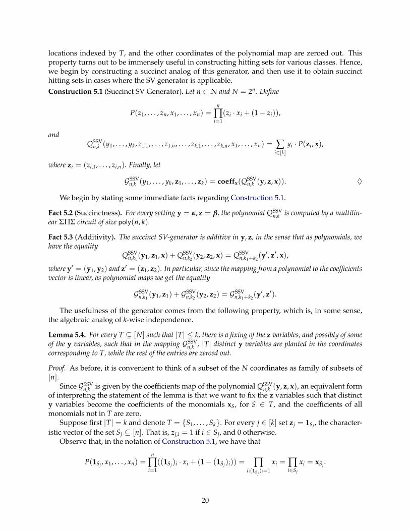
locations indexed by T, and the other coordinates of the polynomial map are zeroed out. Thisproperty turns out to be immensely useful in constructing hitting sets for various classes. Hence,we begin by constructing a succinct analog of this generator, and then use it to obtain succincthitting sets in cases where the SV generator is applicable.Construction 5.1 (Succinct SV Generator). Let n ∈N and N = 2n. Define

P(z1, . . . , zn, x1, . . . , xn) =n

∏i=1

(zi · xi + (1− zi)),

andQSSV

n,k (y1, . . . , yk, z1,1, . . . , z1,n, . . . , zk,1, . . . , zk,n, x1, . . . , xn) = ∑i∈[k]

yi · P(zi, x),

where zi = (zi,1, . . . , zi,n). Finally, let

GSSVn,k (y1, . . . , yk, z1, . . . , zk) = coeffx(QSSV

n,k (y, z, x)). ♦

We begin by stating some immediate facts regarding Construction 5.1.

Fact 5.2 (Succinctness). For every setting y = α, z = β, the polynomial QSSVn,k is computed by a multilin-

ear ΣΠΣ circuit of size poly(n, k).

Fact 5.3 (Additivity). The succinct SV-generator is additive in y, z, in the sense that as polynomials, wehave the equality

QSSVn,k1

(y1, z1, x) + QSSVn,k2

(y2, z2, x) = QSSVn,k1+k2

(y′, z′, x),

where y′ = (y1, y2) and z′ = (z1, z2). In particular, since the mapping from a polynomial to the coefficientsvector is linear, as polynomial maps we get the equality

GSSVn,k1

(y1, z1) + GSSVn,k2

(y2, z2) = GSSVn,k1+k2

(y′, z′).

The usefulness of the generator comes from the following property, which is, in some sense,the algebraic analog of k-wise independence.

Lemma 5.4. For every T ⊆ [N] such that |T| ≤ k, there is a fixing of the z variables, and possibly of someof the y variables, such that in the mapping GSSV

n,k , |T| distinct y variables are planted in the coordinatescorresponding to T, while the rest of the entries are zeroed out.

Proof. As before, it is convenient to think of a subset of the N coordinates as family of subsets of[n].

Since GSSVn,k is given by the coefficients map of the polynomial QSSV

n,k (y, z, x), an equivalent formof interpreting the statement of the lemma is that we want to fix the z variables such that distincty variables become the coefficients of the monomials xS, for S ∈ T, and the coefficients of allmonomials not in T are zero.

Suppose first |T| = k and denote T = S1, . . . , Sk. For every j ∈ [k] set zj = 1Sj , the character-istic vector of the set Sj ⊆ [n]. That is, zj,i = 1 if i ∈ Sj, and 0 otherwise.

Observe that, in the notation of Construction 5.1, we have that

P(1Sj , x1, . . . , xn) =n

∏i=1

((1Sj)i · xi + (1− (1Sj)i)) = ∏i:(1Sj )i=1

xi = ∏i∈Sj

xi = xSj .

20

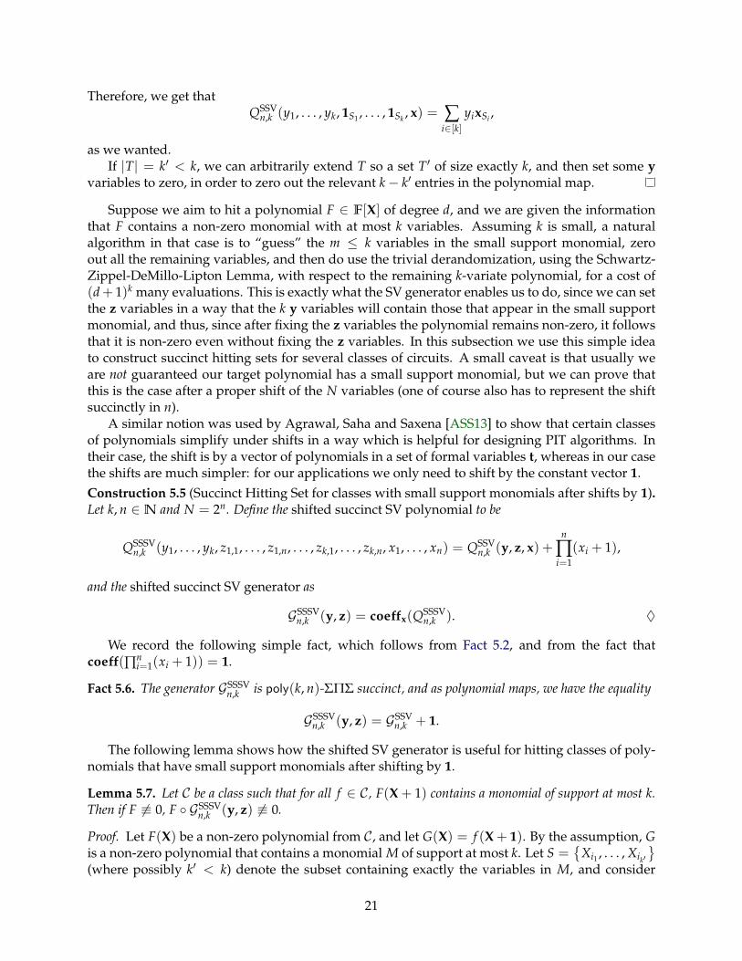
Therefore, we get thatQSSV

n,k (y1, . . . , yk, 1S1 , . . . , 1Sk , x) = ∑i∈[k]

yixSi ,

as we wanted.If |T| = k′ < k, we can arbitrarily extend T so a set T′ of size exactly k, and then set some y

variables to zero, in order to zero out the relevant k− k′ entries in the polynomial map.

Suppose we aim to hit a polynomial F ∈ F[X] of degree d, and we are given the informationthat F contains a non-zero monomial with at most k variables. Assuming k is small, a naturalalgorithm in that case is to “guess” the m ≤ k variables in the small support monomial, zeroout all the remaining variables, and then do use the trivial derandomization, using the Schwartz-Zippel-DeMillo-Lipton Lemma, with respect to the remaining k-variate polynomial, for a cost of(d+ 1)k many evaluations. This is exactly what the SV generator enables us to do, since we can setthe z variables in a way that the k y variables will contain those that appear in the small supportmonomial, and thus, since after fixing the z variables the polynomial remains non-zero, it followsthat it is non-zero even without fixing the z variables. In this subsection we use this simple ideato construct succinct hitting sets for several classes of circuits. A small caveat is that usually weare not guaranteed our target polynomial has a small support monomial, but we can prove thatthis is the case after a proper shift of the N variables (one of course also has to represent the shiftsuccinctly in n).

A similar notion was used by Agrawal, Saha and Saxena [ASS13] to show that certain classesof polynomials simplify under shifts in a way which is helpful for designing PIT algorithms. Intheir case, the shift is by a vector of polynomials in a set of formal variables t, whereas in our casethe shifts are much simpler: for our applications we only need to shift by the constant vector 1.Construction 5.5 (Succinct Hitting Set for classes with small support monomials after shifts by 1).Let k, n ∈N and N = 2n. Define the shifted succinct SV polynomial to be

QSSSVn,k (y1, . . . , yk, z1,1, . . . , z1,n, . . . , zk,1, . . . , zk,n, x1, . . . , xn) = QSSV

n,k (y, z, x) +n

∏i=1

(xi + 1),

and the shifted succinct SV generator as

GSSSVn,k (y, z) = coeffx(QSSSV

n,k ). ♦

We record the following simple fact, which follows from Fact 5.2, and from the fact thatcoeff(∏n

i=1(xi + 1)) = 1.

Fact 5.6. The generator GSSSVn,k is poly(k, n)-ΣΠΣ succinct, and as polynomial maps, we have the equality

GSSSVn,k (y, z) = GSSV

n,k + 1.

The following lemma shows how the shifted SV generator is useful for hitting classes of poly-nomials that have small support monomials after shifting by 1.

Lemma 5.7. Let C be a class such that for all f ∈ C, F(X + 1) contains a monomial of support at most k.Then if F 6≡ 0, F GSSSV

n,k (y, z) 6≡ 0.

Proof. Let F(X) be a non-zero polynomial from C, and let G(X) = f (X + 1). By the assumption, Gis a non-zero polynomial that contains a monomial M of support at most k. Let S =

Xi1 , . . . , Xik′

(where possibly k′ < k) denote the subset containing exactly the variables in M, and consider

21

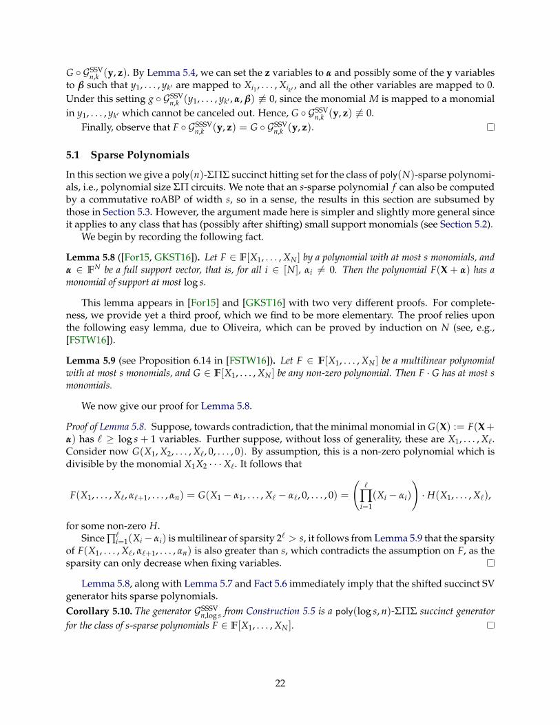
G GSSVn,k (y, z). By Lemma 5.4, we can set the z variables to α and possibly some of the y variables

to β such that y1, . . . , yk′ are mapped to Xi1 , . . . , Xik′, and all the other variables are mapped to 0.

Under this setting g GSSVn,k (y1, . . . , yk′ , α, β) 6≡ 0, since the monomial M is mapped to a monomial

in y1, . . . , yk′ which cannot be canceled out. Hence, G GSSVn,k (y, z) 6≡ 0.

Finally, observe that F GSSSVn,k (y, z) = G GSSV

n,k (y, z).

5.1 Sparse Polynomials

In this section we give a poly(n)-ΣΠΣ succinct hitting set for the class of poly(N)-sparse polynomi-als, i.e., polynomial size ΣΠ circuits. We note that an s-sparse polynomial f can also be computedby a commutative roABP of width s, so in a sense, the results in this section are subsumed bythose in Section 5.3. However, the argument made here is simpler and slightly more general sinceit applies to any class that has (possibly after shifting) small support monomials (see Section 5.2).

We begin by recording the following fact.

Lemma 5.8 ([For15, GKST16]). Let F ∈ F[X1, . . . , XN ] by a polynomial with at most s monomials, andα ∈ FN be a full support vector, that is, for all i ∈ [N], αi 6= 0. Then the polynomial F(X + α) has amonomial of support at most log s.

This lemma appears in [For15] and [GKST16] with two very different proofs. For complete-ness, we provide yet a third proof, which we find to be more elementary. The proof relies uponthe following easy lemma, due to Oliveira, which can be proved by induction on N (see, e.g.,[FSTW16]).

Lemma 5.9 (see Proposition 6.14 in [FSTW16]). Let F ∈ F[X1, . . . , XN ] be a multilinear polynomialwith at most s monomials, and G ∈ F[X1, . . . , XN ] be any non-zero polynomial. Then F · G has at most smonomials.

We now give our proof for Lemma 5.8.

Proof of Lemma 5.8. Suppose, towards contradiction, that the minimal monomial in G(X) := F(X+α) has ` ≥ log s + 1 variables. Further suppose, without loss of generality, these are X1, . . . , X`.Consider now G(X1, X2, . . . , X`, 0, . . . , 0). By assumption, this is a non-zero polynomial which isdivisible by the monomial X1X2 · · ·X`. It follows that

F(X1, . . . , X`, α`+1, . . . , αn) = G(X1 − α1, . . . , X` − α`, 0, . . . , 0) =

(`

∏i=1

(Xi − αi)

)· H(X1, . . . , X`),

for some non-zero H.Since ∏`

i=1(Xi− αi) is multilinear of sparsity 2` > s, it follows from Lemma 5.9 that the sparsityof F(X1, . . . , X`, α`+1, . . . , αn) is also greater than s, which contradicts the assumption on F, as thesparsity can only decrease when fixing variables.

Lemma 5.8, along with Lemma 5.7 and Fact 5.6 immediately imply that the shifted succinct SVgenerator hits sparse polynomials.Corollary 5.10. The generator GSSSV

n,log s from Construction 5.5 is a poly(log s, n)-ΣΠΣ succinct generatorfor the class of s-sparse polynomials F ∈ F[X1, . . . , XN ].

22

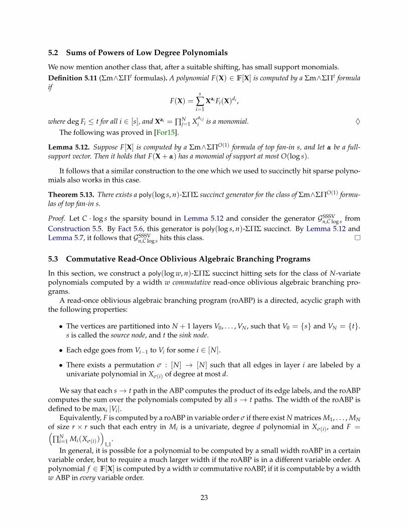
5.2 Sums of Powers of Low Degree Polynomials

We now mention another class that, after a suitable shifting, has small support monomials.Definition 5.11 (Σm∧ΣΠt formulas). A polynomial F(X) ∈ F[X] is computed by a Σm∧ΣΠt formulaif

F(X) =s

∑i=1

Xai Fi(X)di ,

where deg Fi ≤ t for all i ∈ [s], and Xai = ∏Nj=1 X

ai,ji is a monomial. ♦

The following was proved in [For15].

Lemma 5.12. Suppose F[X] is computed by a Σm∧ΣΠO(1) formula of top fan-in s, and let α be a full-support vector. Then it holds that F(X + α) has a monomial of support at most O(log s).

It follows that a similar construction to the one which we used to succinctly hit sparse polyno-mials also works in this case.

Theorem 5.13. There exists a poly(log s, n)-ΣΠΣ succinct generator for the class of Σm∧ΣΠO(1) formu-las of top fan-in s.

Proof. Let C · log s the sparsity bound in Lemma 5.12 and consider the generator GSSSVn,C log s from

Construction 5.5. By Fact 5.6, this generator is poly(log s, n)-ΣΠΣ succinct. By Lemma 5.12 andLemma 5.7, it follows that GSSSV

n,C log s hits this class.

5.3 Commutative Read-Once Oblivious Algebraic Branching Programs

In this section, we construct a poly(log w, n)-ΣΠΣ succinct hitting sets for the class of N-variatepolynomials computed by a width w commutative read-once oblivious algebraic branching pro-grams.

A read-once oblivious algebraic branching program (roABP) is a directed, acyclic graph withthe following properties:

• The vertices are partitioned into N + 1 layers V0, . . . , VN , such that V0 = s and VN = t.s is called the source node, and t the sink node.

• Each edge goes from Vi−1 to Vi for some i ∈ [N].

• There exists a permutation σ : [N] → [N] such that all edges in layer i are labeled by aunivariate polynomial in Xσ(i) of degree at most d.

We say that each s→ t path in the ABP computes the product of its edge labels, and the roABPcomputes the sum over the polynomials computed by all s → t paths. The width of the roABP isdefined to be maxi |Vi|.

Equivalently, F is computed by a roABP in variable order σ if there exist N matrices M1, . . . , MNof size r × r such that each entry in Mi is a univariate, degree d polynomial in Xσ(i), and F =(

∏Ni=1 Mi(Xσ(i))

)1,1

.

In general, it is possible for a polynomial to be computed by a small width roABP in a certainvariable order, but to require a much larger width if the roABP is in a different variable order. Apolynomial f ∈ F[X] is computed by a width w commutative roABP, if it is computable by a widthw ABP in every variable order.

23

Forbes, Saptharishi and Shpilka ([FSS14], Corollary 4.3) showed that in order to hit width-wcommutative roABPs, it is enough to take the SV generator with k = O(log w). 6

We follow the proof strategy of [FSS14] in order to show that the succinct SV generator hitscommutative roABPs as well. The following definitions and the theorem following them are bor-rowed from [FSS14].Definition 5.14. Let g : Fm × Fm′ → FN be a polynomial map. g is said to be an individual degree d,`-wise independent monomial map if for every S ⊆ [N] of size at most `, there is α ∈ Fm′ such that thepolynomials g(t, α)a : supp(a) ⊆ S, maxi ai ≤ d are non-zero and distinct monomials in t, where wedefine

g(t, α)a =N

∏i=1

(g(t, α)aii ). ♦

Definition 5.15 (see also [ASS13]). Let F[X] ∈ F[X]r be a vector of polynomials. We say that F hassupport-k rank concentration at v, if the derivatives of F with respect to all monomials of support at most kat v span all the derivatives of F at v. That is, if

span ∂Xa(F)(v)a:|supp(a)|≤k = span ∂Xa(F)(v)a ♦

Lemma 5.16 ([FSS14], Theorem 4.1). Let F[X] ∈ F[X]w×w be of individual degree d and computed bya commutative roABP of width w. Let g(t, s) be an individual degree d, (log(w2) + 1)-wise independentmonomial map. Then F(X) has support-log(w2) rank concentration at g(t, s) over F(t, s).

The succinct SV generator, like the SV generator, is a k-wise independent monomial map forand degree d.

Lemma 5.17. The polynomial map GSSVn,k (y, z) of Construction 5.1 is an individual degree d, k-wise inde-

pendent monomial map for every d.

Proof. By Lemma 5.4, for any set S of coordinates of size at most k we can set the z variables suchthat each coordinate in S contains a distinct y variable. Then, it is also clear that all individualdegree up to d monomials of this map are distinct, for any choice of d

The final ingredient (also from [FSS14]) is the following lemma, which shows how to obtainhitting sets from rank concentration.

Lemma 5.18 ([FSS14], Corollary 3.5). Let F ∈ F[X]r×r be a matrix of polynomials that is support-k rankconcentrated at α ∈ FN , and let G(X) = F1,1. Then G(X) 6≡ 0 if and only if G (GSSV

n,k + α) 6≡ 0.

We remark that although [FSS14] phrase this lemma for their construction of the SV gener-ator, the proof goes through verbatim using the properties of GSSV

n,k as explained in the proof ofLemma 5.17, and does not depend on the specific implementation.

We now prove that Gn,4 log w+1 hits N-variate polynomials that are computed by width w com-mutative roABPs.

Theorem 5.19. Let |F| > nd, and let F(X) ∈ F[X] be an N-variate polynomial of individual degree atmost d, and computed by a width w commutative roABP. Then, F 6≡ 0 if and only if F GSSV

n,1+4 log w 6≡ 0.6An improved construction for this model, with respect to the size of the hitting set, was given by Gurjar, Korwar

and Saxena [GKS17]. Their construction, however, uses ingredients which we do not know how to make succinct; seeSection 8 for further discussion)

24

Proof. By definition, F is the (1, 1) entry of a matrix polynomial F(X) ∈ F[X]w×w, with F beingcomputed by a width-w commutative roABP. By Lemma 5.17 and Lemma 5.16, we get that thepolynomial F GSSV

n,2 log w+1 is support-log(w2) rank concentrated. By Lemma 5.18, we deduce thatF 6≡ 0 if and only if F (GSSV

n,2 log w+1(y1, z1) + GSSVn,2 log w(y2, z2)) 6≡ 0, where y1, y2, z1, z2 are disjoint

sets of variables. By the additivity property (Fact 5.3), it holds that F 6≡ 0 if and only if F GSSV

n,1+4 log w(y, z) 6≡ 0 for y = (y1, y2) and z = (z1, z2).

Corollary 5.20. There exists a poly(n, log(w))-ΣΠΣ succinct generator for the class of polynomials com-puted by width-w commutative roABPs.

5.4 Depth-D Occur-k Formulas

The following model was considered in [ASSS16].Definition 5.21. An occur-k formula is a directed tree, with internal nodes labeled either by + or ×∧(a power-product gate). The edges entering a ×∧ gate are labeled by integers e1, . . . , em, and on inputsg1, . . . , gm, the gate computes ge1

1 · · · gemm . The leaves of tree are depth-2 formulas which compute sparse

polynomials, such that every variable Xi occur in at most k of them.The size of an occur-k formula is the sum over the sizes of its gates, where

1. The size of a ‘+’ gate is 1,

2. The size of a ‘×∧’ gate is the sum e1 + · · ·+ em of the labels of its incoming edges, and

3. The size of a leaf node is the size of the depth-2 formula it is computing.

The depth of an occur-k formula is the number of layers of + and ×∧ gates, plus 2, to account for thesparse formulas at the leaves. ♦

Agrawal et al. ([ASSS16]) constructed a hitting set for this class, which combines both therank condenser construction (Construction 4.1) and a generator for sparse polynomials. Whilethe original construction uses the Klivans-Spielman generator ([KS01]), it is possible to make thehitting set succinct while using our version of the shifted succinct Shpilka-Volkovich generator.

We now present the succinct generator of depth-D occur-k formulas.

Construction 5.22. Let D, k, n, s ∈ N. Denote R = (2k)2D·2D. For every ` ∈ [D − 2], let y` =

(y`,1, . . . , y`,R) denote a tuple of R variables. We define the polynomial

PASSS(x, y1, . . . , yD−2, t1, . . . , t`, u, v) =D−2

∑`=1GRC

n,R(x1, . . . , xn, y`, t`) + QSSSVn,R log s+R log R(x, u, v),

and the generatorGASSS(y1, . . . , yD−2, t1, . . . , t`, u, v) = coeffx(PASSS). ♦

In our setting, we think of k, D = O(1), which immediately implies:

Fact 5.23. For k, D = O(1), the generator of Construction 5.22 is poly(log s, n)-ΣΠΣ succinct.

We now quote (a variant of) a theorem proved by Agrawal et al., which shows that Construc-tion 5.22 is a generator for depth-D occur-k formulas.

25

Theorem 5.24 ([ASSS16], and see also the presentation in Chapter 4 of [Sap12]). Suppose Φ(w) :Fm → FN is a map such that for any polynomial F(X) ∈ F[X] of sparsity at most R! · sR, F Φ 6≡ 0.Then there exist integers r1, . . . , rD−2 ∈ [R], for R = (2k)2D·2D

such that the map

Ψ : Xi 7→D−2

∑`=1

(r`

∑j=1

yj,`tij`

)+ Φ(w) (5.25)

is a generator for polynomials computed by depth-D occur-k formulas of size s assuming char(F) = 0 orchar(F) > sR.

As a corollary, we obtain that Construction 5.22 is a succinct generator for this class.

Corollary 5.26. For D, k = O(1), Construction 5.22 is a poly(log s, n)-ΣΠΣ succinct generator for theclass of polynomials computed by size-s depth-D occur-k formulas.

Proof. The succinctness claim follows from Fact 5.23.For the hitting property, observe that by Corollary 5.10, the polynomial map GSSSV

n,m (u, v) sat-isfies the properties required from Φ in Theorem 5.24 for m = R log s + R log R, and by Proposi-tion 4.2, the generator

D−2

∑`=1GRC

n,R(y`, t`)

maps every Xi to the polynomial ∑D−2`=1

(∑R

j=1 yj,ltij`

)after using the substitutions in t` to a new

variable t` as given in Proposition 4.2. Since r` ≤ R, the polynomial in (5.25) is a projection ofConstruction 5.22, by possibly restricting excess y` variables to 0.

The claim now follows from Theorem 5.24.

6 Succinct Hitting Sets for Circuits of Sparsely Small TranscendenceDegree

Another model, which was considered in [BMS13], is that of circuits of the form C(F1, . . . , Fm)where the fi’s are polynomials of maximal sparsity s, trdeg F1, . . . , Fm = r and C is an arbitrarycircuit. It is possible to simplify the construction using ideas from [ASSS16], and thus we cite someof the definitions and the lemmas in the latter paper. Since we do not provide full proofs and donot discuss the full background, our terminology is slightly different at certain points.

We begin with the definition of the Jacobian matrix.Definition 6.1. Let F = F1(X), . . . , Fm(X) ⊆ F[X] be a set of N-variate polynomials. The Jacobianmatrix of F, denoted JX(F), is an m× N matrix such that JX(F)i,j = ∂Fi/∂Xj. ♦

The rank of the Jacobian matrix captures the transcendence degree of F, assuming the charac-teristic is 0 or large enough.

Fact 6.2 ([BMS13]). Let F = F1(X), . . . , Fm(X) ⊆ F[X] be a set of N-variate polynomials over F of de-gree at most d, such that trdeg F1, . . . , Fm = r. If char(F) = 0 or char(F) ≥ dr, then rankF(X) JX(F) =r.

This fact shows that a map that preserves the rank of the Jacobian also preserves the tran-scendence degree of the fi’s, a fact which is useful for constructing generators (this is slightlynon-trivial, and see [ASSS16] for details and discussion). For this purpose, we use the following“recipe” from [ASSS16] that gives a construction of such a map.

26

Lemma 6.3 ([ASSS16]). Let F = F1(X), . . . , Fm(X) ⊆ F[X] be a set of N-variate polynomials overF of degree at most d, such that trdeg F1, . . . , Fm ≤ r, and suppose char(F) = 0 or char(F) ≥ dr.Let C(y1, . . . , ym) ∈ F[y] be any polynomial, and let Φ : F[X] → F[z] be a homomorphism such thatrankF(X)(JX(F)) = rankF(z) Φ(JX(F)). Consider the mapping Ψ given by

Xi 7→(

r

∑i=1

yjtij

)+ Φ(Xi).

Then, it holds that C(F1, . . . , Fm) 6≡ 0 if and only if C(Ψ(F1), . . . , Ψ(Fm)) 6≡ 0.

We now show how to construct a succinct generator for circuits of the form C(F1, . . . , Fm) whereFi’s are polynomials of maximal sparsity s, and trdeg F1, . . . , Fm = k.

Lemma 6.4. Let s, r, N ∈N and m = r log s + r log r. Consider the polynomial map

GBMSr,s (y1, . . . , yr, t0, t1, . . . , tn, w1, . . . , wm, z1, . . . , zm) := GRC

n,r (y, t) + GSSSVn,m (w, z).

Let F = F1(X), . . . , Fm(X) ⊆ F[X] be a set of N-variate polynomials over F of sparsity at most s, suchthat trdeg F1, . . . , Fm ≤ r. Then for any polynomial of the form G(x) = C(F1, . . . , Fm), we have thatG 6≡ 0 if and only if G GBMS

r,s 6≡ 0.Furthermore, the generator GBMS

r,s is poly(r, log s, n)-ΣΠΣ succinct.

Proof. By Lemma 6.3 and Proposition 4.2, it is enough to show that the map GSSSVn,m (w, z) preserves

the rank of the Jacobian matrix. This follows from the fact that each r× r minor of this matrix is apolynomial of sparsity at most r! · sr (since taking derivatives can only decrease the sparsity), andfrom Corollary 5.10.

The succinctness claim follows from Proposition 4.2 and Fact 5.6.

Corollary 6.5. There exists a poly(log s, r, n)-ΣΠΣ succinct generator for the class of polynomials of theform C(F1, . . . , Fm) such that each Fi has sparsity at most s and trdeg F1, . . . , Fm ≤ r.

7 Succinct Hitting Sets for Read-Once Oblivious Algebraic BranchingPrograms

In this section we construct a succinct hitting set for the class of read-once oblivious algebraic pro-grams. Recall that in Section 5.3 we have constructed a poly(log w, log n)-ΣΠΣ succinct generatorfor width-w commutative roABPs. For general ABPs, we are only able at this point to constructhitting sets that are width-w2 roABP succinct: i.e., in the hitting set for width w N-variate roABPs,each element is computed by a width w2 n-variate roABP. Ideally, one would want to replace w2

with polylog(w).The definition of roABPs were given in Section 5.3. Throughout this section we assume that

the ABP reads the variables in the order X1, X2, . . . , XN . In Section 7.1 we give some short remarksregarding different variable orderings.

Our construction is based on the following generator by Forbes and Shpilka [FS13].

Lemma 7.1 (Forbes-Shpilka Generator for roABPs, Construction 3.13 in [FS13]). Let n ∈ N andN = 2n. The following polynomial map G : Fn+1 → FN is a generator for width w, individual degree d,N-variate roABPs, in variable order X1, X2, . . . , XN .

27

Let ω ∈ F be of multiplicative order at least (Ndw2)2, and β1, . . . , βw2 be distinct elements of F. Letp` : ` ∈ [w2]

be the Lagrange interpolation polynomials with respect to the βi’s, i.e., pi(β j) = 1 if i = j

and 0 otherwise.Let G : Fn+1 → FN be the following polynomial map, whose output coordinates are indexed by vectors

b ∈ 0, 1n.

GFSb (y) = ∑

`1,...,`n∈[w2]∏

i∈[n]

((1− bi) · p`i−1(ω

`i yi) + bi · p`i−1((ω`i yi)

2i−1dw2))· p`n(yn+1), (7.2)

where we abuse notation by defining p`0(t) = t.

In [FS13] (Lemma 3.18), it is shown that this map, for every fixed output coordinate b, iscomputed by a width w2 roABP in the variables y. We, however, want to show that for everyfixing y = α, there is a small roABP computing the polynomial whose coefficient vector is givenby (Gb(α))b∈0,1n . That is, for every choice of α, and associating b with a subset of [n], we want apolynomial in x1, . . . , xn such that the coefficient of xb is Gb(α).Definition 7.3 (Succinct Forbes-Shpilka Generator). Let n, w ∈N, and ω, pi’s as in Lemma 7.1. Define

PFS(x1, . . . , xn, y1, . . . , yn+1) = ∑`1,...,`n∈[w2]

∏i∈[n]

(p`i−1(ω

`i yi)

+ xi · p`i−1((ω`i yi)

2i−1dw2))· p`n(yn+1). ♦

We first claim the the Forbes-Shpilka generator (7.2) is given by the coefficient vector of thispolynomial.

Claim 7.4. Assume the setup and notations of Definition 7.3. Then coeffx(PFS) = GFS.

Proof. As explained earlier, we wish to show that the coefficient of xb in the polynomial PFS equalsthe b-th coordinate of (7.2).

Fix a choice of `1, . . . , `n ∈ [w2], and b ∈ 0, 1n. Consider the product

∏i∈[n]

(p`i−1(ω

`i yi) + xi · p`i−1((ω`i yi)

2i−1dw2))

.

Since the product is over distinct variables, there is exactly one way to obtain the monomial xb =

∏i:bi=1 xi in this product, and its coefficient will be

∏i:bi=1

p`i−1((ω`i yi)

2i−1dw2) · ∏

i:bi=0p`i−1(ω

`i yi) (7.5)

Finally, observe that (7.5) exactly equals

∏i∈[n]

((1− bi) · p`i−1(ω

`i yi) + bi · p`i−1((ω`i yi)

2i−1dw2))

.

This is true for every fixed choice of `1, . . . , `n, and the claim now follows from the linearity of thecoefficients map.

We now show that for every fixing y = α, the polynomial PFS(x, α) is computed by a smallroABP.

28

Claim 7.6. For every setting y = α, the polynomial PFS(x, α) in Definition 7.3 can be computed by awidth w2 roABP in variable order x1, x2 . . . , xn.

Proof. The construction is straightforward from Definition 7.3. Layer V0 contains the source vertexs and layer Vn+1 the sink vertex t. Layers V1, . . . , Vn each contain w2 vertices labeled by the set [w2].For every i ∈ [n] and every ` ∈ Vi, there is an edge from each vertex in the previous layer, labeledby the linear function (in xi)

p`i−1(ω`i αi) + xi · p`i−1((ω

`i αi)2i−1dw2

).

Finally, all vertices in Vn are connected to t with an edge labeled p`n(αn+1).

Corollary 7.7. The Forbes-Shpilka generator given in Lemma 7.1 is a width w2-roABP succinct generatorfor degree d roABPs that read the variables in order X1, X2, . . . , XN .

Proof. Immediate from Lemma 7.1, Claim 7.4 and Claim 7.6.

7.1 Different Variable Orderings

The generator given by Forbes and Shpilka in Lemma 7.1 hits roABPs that read the variables inthe order X1, X2, . . . , XN and not necessarily in any variable order. Obviously, we can apply apermutation σ to the variables x1, . . . , xn in Definition 7.3 to obtain a roABP in the variables xin the order σ: the coefficient vector of this roABP hits roABPs in the variables X that read theirvariables in the order on X1, . . . , XN which is given by considering the lexicographic orderinginduced on the set of multilinear monomials in x1, . . . , xn by the order σ, and using the canonicalidentification of a multilinear monomial with an index in [N], say, using the binary representation.We call such an order relation on [N] a monomial-compatible ordering. Note that there are merelyn! such orderings among the N! total orderings on [N].

Since in our case we do not care about the size of the hitting set, we can take the union of all n!those succinct hitting sets to obtain the following corollary.Corollary 7.8. There exists a width-w2 roABP succinct hitting set for the class of width w, N variate, anddegree d roABPs that read the variables in a monomial compatible ordering.

8 Discussion and Open Problems

In this work, we have shown that many of the hitting sets we know for restricted algebraic modelsof computation can be represented in a succinct form as coefficient vectors of small circuits. Thisgives some positive answers to Meta-Conjecture 1.8, and points to the possibility of an algebraicnatural proofs barrier. The main problem left open by this work is to construct succinct hittingsets for stronger models for which we know how to construct hitting sets efficiently.

For example, while we were able to construct a succinct generator for commutative roABPs,our construction for general roABPs is not fully succinct, and also works only in certain variableorderings. Despite several works that obtain quasi-polynomial size hitting sets for roABPs in anyorder ([FSS14, AGKS15]), none of them seems to fit easily into the succinct setting, each for its ownreasons.

For bounded-depth multilinear formulas, subexponential size hitting sets were obtained byOliveira, Shpilka and Volk [OSV16]. The construction there can be roughly described as hashingthe N variables into N1−ε buckets, and then hitting each bucket independently using a generatorfor roABPs (in fact, commutative roABPs will suffice). The main challenge here seems to be the

29

hashing part, which (in the succinct setting) would involve hashing monomials, and ensuring thatthe coefficient vector that is obtained through this process has a small circuit for any possible hashfunction.

The main technical tool which we do not know how to emulate in the succinct setting is theKlivans-Spielman [KS01] generator. In this generator, the variable Xi is mapped to tki mod p, wheret is a new indeterminate, p is chosen from an appropriately large set of primes and k from anappropriately large set of natural numbers. The main feature of this generator is that given a“small” enough set of monomialsM, the parameters k, p can be chosen from a “not too large” set,such that all the monomials inM are given distinct weights, and this can be done in a black-boxmanner, that is, without knowingM, but only an upper bound on its size. Indeed, the noticeabledifference from the constructions we have given in this paper is the exponential dependence on iin the exponent of t, a feature which is not clear how to emulate in the succinct setting.

The main application of the Klivans and Spielman construction is to construct hitting sets forsparse polynomials. While we are unable to make the resulting hitting set succinct, we devel-oped an alternate hitting set which we succeeded in making succinct. However, the Klivans andSpielman construction (or otherwise similar ideas) has also found applications beyond the class ofsparse polynomials, such as in the construction hitting sets for roABPs in unknown order from thework of Agrawal, Gurjar, Korwar and Saxena [AGKS15]. Unfortunately, such works seem to relyheavily on properties of the Klivans and Spielman construction beyond that of just hitting sparsepolynomials, and as such we are currently unable to make these hitting sets succinct.

A particular interesting application of the Klivans and Spielman construction is in the re-cent works of Fenner, Gurjar and Thierauf [FGT16] and its generalization by Gurjar and Thierauf[GT17]. These works construct hitting sets for the class of determinants of “read-once matrices”,which are polynomials of the form det M, where M is a matrix in which each entry contains a vari-able xi,j or a field constant, and each variable appears at most once in the matrix. While this class ofpolynomials is very restricted, the partial derivative matrix used by Nisan [Nis91a], Raz [Raz09],and Raz-Yehudayoff [RY09], is a read-once matrix. As such, the lower bounds proved in thesepapers are algebraically natural and the distinguisher used is a read-once determinant. The workof Raz and Yehudayoff [RY09] in particular shows that a read-once determinant can vanish onthe coefficient vectors of constant-depth multilinear formulas, and as most of the constructions inthis paper have this form this shows that these constructions cannot be succinct hitting sets forread-once determinants, and hence new ideas are needed. Indeed, if one could establish a circuitclass C where there are C-succinct hitting sets for read-once determinants then this would showthat no proof technique following the ideas of the above works can prove lower bounds for theclass C. Such a result would be very interesting as those lower bounds methods are still very muchstate-of-the-art.

As mentioned earlier, stronger evidence towards an algebraic natural proofs barrier can alsobe obtained by designing pseudorandom polynomials whose security is based on widely-believedcryptographic assumptions. In particular, one possible approach is obtaining evidence in favor ofthe determinant-based construction of Aaronson and Drucker [AD08].

Acknowledgements

We thank Scott Aaronson, Andy Drucker, Josh Grochow, Mrinal Kumar, Shubhangi Saraf and DorMinzer for useful conversations regarding this work. We also thank the anonymous reviewers fortheir careful reading of this paper and for many useful comments.

30

References

[Aar16] Scott Aaronson. P ?= NP. In Open Problems in Mathematics, pages 1–122. Springer, 2016.

[AB87] Noga Alon and Ravi B. Boppana. The monotone circuit complexity of Boolean func-tions. Combinatorica, 7(1):1–22, 1987.

[AD08] Scott Aaronson and Andrew Drucker. Arithmetic natural proofs theory is sought.Blog post, http://www.scottaaronson.com/blog/?p=336, 2008.

[AGHP92] Noga Alon, Oded Goldreich, Johan Hastad, and Rene Peralta. Simple Construction ofAlmost k-wise Independent Random Variables. Random Struct. Algorithms, 3(3):289–304, 1992. Preliminary version in the 31st Annual IEEE Symposium on Foundations ofComputer Science (FOCS 1990).

[AGKS15] Manindra Agrawal, Rohit Gurjar, Arpita Korwar, and Nitin Saxena. Hitting-Sets forROABP and Sum of Set-Multilinear Circuits. SIAM J. Comput., 44(3):669–697, 2015.Pre-print available at arXiv:1406.7535.

[Agr05] Manindra Agrawal. Proving Lower Bounds Via Pseudo-random Generators. In Pro-ceedings of the 25th International Conference on Foundations of Software Technology andTheoretical Computer Science (FSTTCS 2005), pages 92–105, 2005.

[AJMV98] Eric Allender, Jia Jiao, Meena Mahajan, and V. Vinay. Non-Commutative ArithmeticCircuits: Depth Reduction and Size Lower Bounds. Theoretical Computer Science, 209(1-2):47–86, 1998. Pre-print available at eccc:TR95-043.

[Ajt83] Miklos Ajtai. Σ11-formulae on finite structures. Annals of pure and applied logic, 24(1):1–

48, 1983.

[ASS13] Manindra Agrawal, Chandan Saha, and Nitin Saxena. Quasi-polynomial hitting-setfor set-depth-∆ formulas. In Proceedings of the 45th Annual ACM Symposium on Theoryof Computing (STOC 2013), pages 321–330, 2013. Full version at arXiv:1209.2333.

[ASSS16] Manindra Agrawal, Chandan Saha, Ramprasad Saptharishi, and Nitin Saxena. Jaco-bian Hits Circuits: Hitting Sets, Lower Bounds for Depth-D Occur-k Formulas andDepth-3 Transcendence Degree-k Circuits. SIAM J. Comput., 45(4):1533–1562, 2016.Preliminary version in the 44th Annual ACM Symposium on Theory of Computing (STOC2012).

[AV08] Manindra Agrawal and V. Vinay. Arithmetic Circuits: A Chasm at Depth Four. In Pro-ceedings of the 49th Annual IEEE Symposium on Foundations of Computer Science (FOCS2008), pages 67–75, 2008. Pre-print available at eccc:TR08-062.

[AW09] Scott Aaronson and Avi Wigderson. Algebrization: A New Barrier in ComplexityTheory. TOCT, 1(1):2:1–2:54, 2009.

[BCS97] Peter Burgisser, Michael Clausen, and Mohammad A. Shokrollahi. Algebraic Com-plexity Theory, volume 315 of Grundlehren der mathematischen Wissenschaften. Springer-Verlag, 1997.

[Ber84] Stuart J. Berkowitz. On computing the determinant in small parallel time using asmall number of processors. Information Processing Letters, 18(3):147 – 150, 1984.

31

[BGS75] Theodore P. Baker, John Gill, and Robert Solovay. Relativizations of the P =? NPQuestion. SIAM J. Comput., 4(4):431–442, 1975.

[BIJL18] Markus Blaser, Christian Ikenmeyer, Gorav Jindal, and Vladimir Lysikov. Generalizedmatrix completion and algebraic natural proofs. In Proceedings of the 50th Annual ACMSymposium on Theory of Computing (STOC 2018), pages 1193–1206, 2018.

[BIZ17] Karl Bringmann, Christian Ikenmeyer, and Jeroen Zuiddam. On Algebraic BranchingPrograms of Small Width. In Proceedings of the 32nd Annual Computational ComplexityConference (CCC 2017), pages 20:1–20:31, 2017.

[Bla14] Markus Blaser. Explicit tensors. In Perspectives in Computational Complexity, pages117–130. Springer, 2014.

[BMS13] Malte Beecken, Johannes Mittmann, and Nitin Saxena. Algebraic independence andblackbox identity testing. Inf. Comput., 222:2–19, 2013. Preliminary version in the 38thInternational Colloquium on Automata, Languages and Programming (ICALP 2011).

[Bra10] Mark Braverman. Polylogarithmic independence fools AC0 circuits. J. ACM,57(5):28:1–28:10, 2010. Preliminary version in the 24th Annual IEEE Conference on Com-putational Complexity (CCC 2009). Pre-print available at eccc:TR09-011.

[BS83] Walter Baur and Volker Strassen. The Complexity of Partial Derivatives. TheoreticalComputer Science, 22:317–330, 1983.

[Bur00] Peter Burgisser. Completeness and Reduction in Algebraic Complexity Theory. Algorithmsand Computation in Mathematics. Springer, 2000.

[Cho11] Timothy Y. Chow. Almost-natural proofs. J. Comput. Syst. Sci., 77(4):728–737, 2011.

[CIKK16] Marco L. Carmosino, Russell Impagliazzo, Valentine Kabanets, and AntoninaKolokolova. Learning Algorithms from Natural Proofs. In Proceedings of the 31st An-nual Computational Complexity Conference (CCC 2016), pages 10:1–10:24, 2016.

[CKSV16] Suryajith Chillara, Mrinal Kumar, Ramprasad Saptharishi, and V. Vinay. The Chasmat Depth Four, and Tensor Rank : Old results, new insights. Electronic Colloquium onComputational Complexity (ECCC), 23:96, 2016.

[CW15] Brynmor Chapman and Ryan Williams. The Circuit-Input Game, Natural Proofs, andTesting Circuits With Data. In Proceedings of the 6th Conference on Innovations in Theo-retical Computer Science (ITCS 2015), pages 263–270, 2015.

[DL78] Richard A. DeMillo and Richard J. Lipton. A Probabilistic Remark on Algebraic Pro-gram Testing. Information Processing Letters, 7(4):193–195, 1978.

[DS07] Zeev Dvir and Amir Shpilka. Locally Decodable Codes with Two Queries and Poly-nomial Identity Testing for Depth 3 Circuits. SIAM J. Comput., 36(5):1404–1434, 2007.Preliminary version in the 37th Annual ACM Symposium on Theory of Computing (STOC2005).

[DSY09] Zeev Dvir, Amir Shpilka, and Amir Yehudayoff. Hardness-Randomness Tradeoffs forBounded Depth Arithmetic Circuits. SIAM J. Comput., 39(4):1279–1293, 2009.

32

[EGOW18] Klim Efremenko, Ankit Garg, Rafael Oliveira, and Avi Wigderson. Barriers for RankMethods in Arithmetic Complexity. In Proceedings of the 9th Conference on Innovations inTheoretical Computer Science (ITCS 2018), volume 94 of Leibniz International Proceedingsin Informatics (LIPIcs), pages 1:1–1:19, 2018.

[FG15] Michael A. Forbes and Venkatesan Guruswami. Dimension Expanders via Rank Con-densers. In Proceedings of the 19th International Workshop on Randomization and Com-putation (RANDOM 2015), volume 40 of LIPIcs, pages 800–814, 2015. Full version atarXiv:1411.7455.

[FGT16] Stephen A. Fenner, Rohit Gurjar, and Thomas Thierauf. Bipartite perfect matching isin quasi-NC. In Proceedings of the 48th Annual ACM Symposium on Theory of Computing(STOC 2016), pages 754–763. ACM, 2016.

[FLMS14] Herve Fournier, Nutan Limaye, Guillaume Malod, and Srikanth Srinivasan. Lowerbounds for depth 4 formulas computing iterated matrix multiplication. In Proceedingsof the 46th Annual ACM Symposium on Theory of Computing (STOC 2014), pages 128–135,2014. Pre-print available at eccc:TR13-100.

[For15] Michael A. Forbes. Deterministic Divisibility Testing via Shifted Partial Derivatives.In Proceedings of the 56th Annual IEEE Symposium on Foundations of Computer Science(FOCS 2015), pages 451–465. IEEE Computer Society, 2015.

[FS12] Michael A. Forbes and Amir Shpilka. On Identity Testing of Tensors, Low-rank Recov-ery and Compressed Sensing. In Proceedings of the 44th Annual ACM Symposium on The-ory of Computing (STOC 2012), pages 163–172, 2012. Full version at arXiv:1111.0663.

[FS13] Michael A. Forbes and Amir Shpilka. Quasipolynomial-Time Identity Testing of Non-commutative and Read-Once Oblivious Algebraic Branching Programs. In Proceedingsof the 54th Annual IEEE Symposium on Foundations of Computer Science (FOCS 2013),pages 243–252, 2013. Full version at arXiv:1209.2408.

[FSS84] Merrick L. Furst, James B. Saxe, and Michael Sipser. Parity, Circuits, and thePolynomial-Time Hierarchy. Mathematical Systems Theory, 17(1):13–27, 1984.

[FSS14] Michael A. Forbes, Ramprasad Saptharishi, and Amir Shpilka. Hitting sets for multi-linear read-once algebraic branching programs, in any order. In Proceedings of the 46thAnnual ACM Symposium on Theory of Computing (STOC 2014), pages 867–875, 2014.

[FSTW16] Michael A. Forbes, Amir Shpilka, Iddo Tzameret, and Avi Wigderson. Proof Com-plexity Lower Bounds from Algebraic Circuit Complexity. In Proceedings of the 31stAnnual Computational Complexity Conference (CCC 2016), pages 32:1–32:17, 2016. Pre-print available at arXiv:1606.05050.

[GGM86] Oded Goldreich, Shafi Goldwasser, and Silvio Micali. How to construct random func-tions. J. ACM, 33(4):792–807, 1986.

[GKKS14] Ankit Gupta, Pritish Kamath, Neeraj Kayal, and Ramprasad Saptharishi. Approach-ing the Chasm at Depth Four. J. ACM, 61(6):33:1–33:16, 2014.

[GKKS16] Ankit Gupta, Pritish Kamath, Neeraj Kayal, and Ramprasad Saptharishi. ArithmeticCircuits: A Chasm at Depth 3. SIAM J. Comput., 45(3):1064–1079, 2016.

33

[GKS17] Rohit Gurjar, Arpita Korwar, and Nitin Saxena. Identity Testing for Constant-Width,and Any-Order, Read-Once Oblivious Arithmetic Branching Programs. Theory of Com-puting, 13(1):1–21, 2017.

[GKSS17] Joshua A. Grochow, Mrinal Kumar, Michael Saks, and Shubhangi Saraf. To-wards an algebraic natural proofs barrier via polynomial identity testing. CoRR,abs/1701.01717, 2017.

[GKST16] Rohit Gurjar, Arpita Korwar, Nitin Saxena, and Thomas Thierauf. Deterministic Iden-tity Testing for Sum of Read-Once Oblivious Arithmetic Branching Programs. Compu-tational Complexity, pages 1–46, 2016. Pre-print available at arXiv:1411.7341.

[GMQ16] Joshua A. Grochow, Ketan D. Mulmuley, and Youming Qiao. Boundaries of VP andVNP. In Proceedings of the 43rd International Colloquium on Automata, Languages andProgramming (ICALP 2016), volume 55 of LIPIcs, pages 34:1–34:14, 2016. Full versionat arXiv:abs/1605.02815.

[GR08] Ariel Gabizon and Ran Raz. Deterministic extractors for affine sources over largefields. Combinatorica, 28(4):415–440, 2008. Preliminary version in the 46th Annual IEEESymposium on Foundations of Computer Science (FOCS 2005).

[Gro15] Joshua A. Grochow. Unifying Known Lower Bounds via Geometric Complexity The-ory. Computational Complexity, 24(2):393–475, 2015. Preliminary version in the 29thAnnual IEEE Conference on Computational Complexity (CCC 2014).

[GT17] Rohit Gurjar and Thomas Thierauf. Linear matroid intersection is in quasi-NC. InProceedings of the 49th Annual ACM Symposium on Theory of Computing (STOC 2017),pages 821–830, 2017. Full version in the Electronic Colloquium on ComputationalComplexity (ECCC), Technical Report TR16-182.

[Has89] Johan Hastad. Almost Optimal Lower Bounds for Small Depth Circuits. In Random-ness and Computation, pages 6–20. JAI Press, 1989.

[HILL99] Johan Hastad, Russell Impagliazzo, Leonid A. Levin, and Michael Luby. A Pseudo-random Generator from any One-way Function. SIAM J. Comput., 28(4):1364–1396,1999.

[HS65] Juris Hartmanis and Richard E. Stearns. On the Computational Complexity of Algo-rithms. Transactions of the American Mathematical Society, 117:285–306, 1965.

[HS80] Joos Heintz and Claus-Peter Schnorr. Testing Polynomials which Are Easy to Com-pute (Extended Abstract). In Proceedings of the 12th Annual ACM Symposium on Theoryof Computing (STOC 1980), pages 262–272, 1980.

[Kay12] Neeraj Kayal. An exponential lower bound for the sum of powers of bounded degreepolynomials. In Electronic Colloquium on Computational Complexity (ECCC)TR12-081,2012.

[KI04] Valentine Kabanets and Russell Impagliazzo. Derandomizing Polynomial IdentityTests Means Proving Circuit Lower Bounds. Computational Complexity, 13(1-2):1–46,2004. Preliminary version in the 35th Annual ACM Symposium on Theory of Computing(STOC 2003).

34

[KL82] Richard M. Karp and Richard J. Lipton. Turing machines that take advice.L’Enseignement Mathematique, 28(2):191–209, 1982.

[KL01] Matthias Krause and Stefan Lucks. Pseudorandom functions in TC0 and crypto-graphic limitations to proving lower bounds. Computational Complexity, 10(4):297–313,2001.

[KLSS14] Neeraj Kayal, Nutan Limaye, Chandan Saha, and Srikanth Srinivasan. An Exponen-tial Lower Bound for Homogeneous Depth Four Arithmetic Circuits. In Proceedings ofthe 55th Annual IEEE Symposium on Foundations of Computer Science (FOCS 2014), pages61–70, 2014. Pre-print available at eccc:TR14-005.

[Koi12] Pascal Koiran. Arithmetic Circuits: The Chasm at Depth Four Gets Wider. TheoreticalComputer Science, 448:56–65, 2012. Pre-print available at arXiv:1006.4700.

[KS01] Adam Klivans and Daniel A. Spielman. Randomness efficient identity testing of mul-tivariate polynomials. In Proceedings of the 33rd Annual ACM Symposium on Theory ofComputing (STOC 2001), pages 216–223, 2001.

[KS09] Neeraj Kayal and Shubhangi Saraf. Blackbox polynomial identity testing for depth-3circuits. In Proceedings of the 50th Annual IEEE Symposium on Foundations of ComputerScience (FOCS 2009), 2009.

[KS11] Zohar Shay Karnin and Amir Shpilka. Black box polynomial identity testing of gener-alized depth-3 arithmetic circuits with bounded top fan-in. Combinatorica, 31(3):333–364, 2011. Preliminary version in the 23rd Annual IEEE Conference on ComputationalComplexity (CCC 2008).

[KS14] Mrinal Kumar and Shubhangi Saraf. On the power of homogeneous depth 4 arith-metic circuits. In Proceedings of the 55th Annual IEEE Symposium on Foundations of Com-puter Science (FOCS 2014), pages 364–373, 2014. Pre-print available at eccc:TR14-045.

[KSS14] Neeraj Kayal, Chandan Saha, and Ramprasad Saptharishi. A super-polynomial lowerbound for regular arithmetic formulas. In Proceedings of the 46th Annual ACM Sympo-sium on Theory of Computing (STOC 2014), pages 146–153, 2014. Pre-print available ateccc:TR13-091.

[LFKN92] Carsten Lund, Lance Fortnow, Howard J. Karloff, and Noam Nisan. Algebraic Meth-ods for Interactive Proof Systems. J. ACM, 39(4):859–868, 1992.

[MS01] Ketan D Mulmuley and Milind Sohoni. Geometric complexity theory I: An approachto the P vs. NP and related problems. SIAM J. Comput., 31(2):496–526, 2001.

[Mul12] Ketan Mulmuley. Geometric Complexity Theory V: Equivalence between BlackboxDerandomization of Polynomial Identity Testing and Derandomization of Noether’sNormalization Lemma. In Proceedings of the 53rd Annual IEEE Symposium on Founda-tions of Computer Science (FOCS 2012), pages 629–638, 2012.

[MV97] Meena Mahajan and V. Vinay. A Combinatorial Algorithm for the Determinant. In Pro-ceedings of the 8th Annual ACM-SIAM Symposium on Discrete Algorithms (SODA 1997),pages 730–738, 1997. Available on citeseer:10.1.1.31.1673.

35

[Nis91a] Noam Nisan. Lower bounds for non-commutative computation. In Proceedings ofthe 23rd Annual ACM Symposium on Theory of Computing (STOC 1991), pages 410–418,1991. Available on citeseer:10.1.1.17.5067.

[Nis91b] Noam Nisan. Pseudorandom bits for constant depth circuits. Combinatorica, 11(1):63–70, 1991.

[Nis92] Noam Nisan. Pseudorandom generators for space-bounded computation. Combina-torica, 12(4):449–461, 1992.

[NN93] Joseph Naor and Moni Naor. Small-Bias Probability Spaces: Efficient Constructionsand Applications. SIAM J. Comput., 22(4):838–856, 1993. Preliminary version in the22nd Annual ACM Symposium on Theory of Computing (STOC 1990).

[NR97] Moni Naor and Omer Reingold. Number-theoretic Constructions of Efficient Pseudo-random Functions. In Proceedings of the 38th Annual IEEE Symposium on Foundations ofComputer Science (FOCS 1997), pages 458–467. IEEE Computer Society, 1997.

[NW94] Noam Nisan and Avi Wigderson. Hardness vs Randomness. J. Comput. Syst. Sci.,49(2):149–167, 1994. Available on citeseer:10.1.1.83.8416.

[NW97] Noam Nisan and Avi Wigderson. Lower bounds on arithmetic circuits viapartial derivatives. Computational Complexity, 6(3):217–234, 1997. Available onciteseer:10.1.1.90.2644.

[OSV16] Rafael Oliveira, Amir Shpilka, and Ben Lee Volk. Subexponential Size Hitting Setsfor Bounded Depth Multilinear Formulas. Computational Complexity, 25(2):455–505,2016. Preliminary version in the 30th Annual Computational Complexity Conference (CCC2015).

[Raz85] Alexander A Razborov. Lower bounds on the monotone complexity of some Booleanfunctions. In Dokl. Akad. Nauk SSSR, volume 281(4), pages 798–801, 1985. Translationin Soviet Math. Doklady, 31, 354–357.

[Raz87] Alexander A. Razborov. Lower bounds on the size of bounded depth circuits over acomplete basis with logical addition. Mathematical notes of the Academy of Sciences of theUSSR, 41(4):333–338, 1987.

[Raz06] Ran Raz. Separation of Multilinear Circuit and Formula Size. Theory of Computing,2(1):121–135, 2006. Preliminary version in the 45th Annual IEEE Symposium on Foun-dations of Computer Science (FOCS 2004). Pre-print available at eccc:TR04-042.

[Raz09] Ran Raz. Multi-Linear Formulas for Permanent and Determinant are of Super-Polynomial Size. J. ACM, 56(2):8:1–8:17, 2009. Preliminary version in the 36th An-nual ACM Symposium on Theory of Computing (STOC 2004). Pre-print available ateccc:TR03-067.

[Raz10] Ran Raz. Elusive Functions and Lower Bounds for Arithmetic Circuits. Theory ofComputing, 6(1):135–177, 2010.

[RR97] Alexander A. Razborov and Steven Rudich. Natural Proofs. J. Comput. Syst. Sci.,55(1):24–35, 1997.

36

[RY08] Ran Raz and Amir Yehudayoff. Balancing Syntactically Multilinear Arithmetic Cir-cuits. Computational Complexity, 17(4):515–535, 2008.

[RY09] Ran Raz and Amir Yehudayoff. Lower Bounds and Separations for Constant DepthMultilinear Circuits. Computational Complexity, 18(2):171–207, 2009. Preliminary ver-sion in the 23rd Annual IEEE Conference on Computational Complexity (CCC 2008). Pre-print available at eccc:TR08-006.

[Sap12] Ramprasad Saptharishi. Unified Approaches to Polynomial Identity Testing and LowerBounds. PhD thesis, Chennai Mathematical Institute, 2012.

[Sap16] Ramprasad Saptharishi. A survey of lower bounds in arithmetic circuit complexity.Github survey, https://github.com/dasarpmar/lowerbounds-survey/, 2016.

[Sax09] Nitin Saxena. Progress on Polynomial Identity Testing. Bulletin of the EATCS, (99):49–79, 2009.

[Sax14] Nitin Saxena. Progress on Polynomial Identity Testing - II. In Perspectives in Com-putational Complexity: The Somenath Biswas Anniversary Volume, pages 131–146, 2014.Pre-print available at eccc:TR13-186.

[Sch80] Jacob T. Schwartz. Fast Probabilistic Algorithms for Verification of Polynomial Iden-tities. J. ACM, 27(4):701–717, 1980.

[Sha90] Adi Shamir. IP=PSPACE. In Proceedings of the 31st Annual IEEE Symposium on Founda-tions of Computer Science (FOCS 1990), pages 11–15, 1990.

[Smo87] Roman Smolensky. Algebraic Methods in the Theory of Lower Bounds for BooleanCircuit Complexity. In Proceedings of the 19th Annual ACM Symposium on Theory ofComputing (STOC 1987), pages 77–82, 1987.

[SS11] Nitin Saxena and C. Seshadhri. An Almost Optimal Rank Bound for Depth-3 Iden-tities. SIAM J. Comput., 40(1):200–224, 2011. Preliminary version in the 24th AnnualIEEE Conference on Computational Complexity (CCC 2009).

[SS12] Nitin Saxena and C. Seshadhri. Blackbox Identity Testing for Bounded Top-FaninDepth-3 Circuits: The Field Doesn’t Matter. SIAM J. Comput., 41(5):1285–1298, 2012.Preliminary version in the 43rd Annual ACM Symposium on Theory of Computing (STOC2011).

[SS13] Nitin Saxena and C. Seshadhri. From sylvester-gallai configurations to rank bounds:Improved blackbox identity test for depth-3 circuits. J. ACM, 60(5):33, 2013. Prelim-inary version in the 51st Annual IEEE Symposium on Foundations of Computer Science(FOCS 2010).

[Str73] Volker Strassen. Die Berechnungskomplexitat Von Elementarsymmetrischen Funktio-nen Und Von Interpolationskoeffizienten. Numerische Mathematik, 20(3):238–251, June1973.

[SV15] Amir Shpilka and Ilya Volkovich. Read-once polynomial identity testing. Computa-tional Complexity, 24(3):477–532, 2015. Preliminary version in the 40th Annual ACMSymposium on Theory of Computing (STOC 2008).

37

[SY10] Amir Shpilka and Amir Yehudayoff. Arithmetic Circuits: A survey of recent resultsand open questions. Foundations and Trends in Theoretical Computer Science, 5:207–388,March 2010.

[Tar88] Eva Tardos. The gap between monotone and non-monotone circuit complexity is ex-ponential. Combinatorica, 8(1):141–142, 1988.

[Tav15] Sebastien Tavenas. Improved bounds for reduction to depth 4 and depth 3. Inf. Com-put., 240:2–11, 2015. Preliminary version in the 38th Internationl Symposium on the Math-ematical Foundations of Computer Science (MFCS 2013).

[Val79] Leslie G. Valiant. Completeness Classes in Algebra. In Proceedings of the 11th AnnualACM Symposium on Theory of Computing (STOC 1979), pages 249–261, 1979.

[VSBR83] Leslie G. Valiant, Sven Skyum, S. Berkowitz, and Charles Rackoff. Fast Parallel Com-putation of Polynomials Using Few Processors. SIAM J. Comput., 12(4):641–644, 1983.Preliminary version in the 6th Internationl Symposium on the Mathematical Foundationsof Computer Science (MFCS 1981).

[Wil14] Ryan Williams. Nonuniform ACC Circuit Lower Bounds. J. ACM, 61(1):2:1–2:32, 2014.

[Wil16] R. Ryan Williams. Natural Proofs versus Derandomization. SIAM J. Comput.,45(2):497–529, 2016.

[Yao85] Andrew Chi-Chih Yao. Separating the Polynomial-Time Hierarchy by Oracles (Pre-liminary Version). In Proceedings of the 26th Annual IEEE Symposium on Foundations ofComputer Science (FOCS 1985), pages 1–10, 1985.

[Zip79] Richard Zippel. Probabilistic algorithms for sparse polynomials. In Symbolic and Alge-braic Computation, EUROSAM ’79, An International Symposiumon Symbolic and AlgebraicComputation, volume 72 of Lecture Notes in Computer Science, pages 216–226. Springer,1979.

38