
SUBSPACE SYSTEM IDENTIFICATION Theory and...
282
SUBSPACE SYSTEM IDENTIFICATION Theory and applications Lecture notes Dr. ing. David Di Ruscio Telemark Institute of Technology Email: [email protected] Porsgrunn, Norway January 1995 6th edition December 11, 2009 Telemark University College Kjølnes Ring 56 N-3914 Porsgrunn, Norway
Transcript of SUBSPACE SYSTEM IDENTIFICATION Theory and...
SUBSPACE SYSTEM IDENTIFICATIONTheory and applications
Lecture notes
Dr. ing.David Di Ruscio
Telemark Institute of TechnologyEmail: [email protected]
Porsgrunn, Norway
January 1995
6th edition December 11, 2009 Telemark University CollegeKjølnes Ring 56N-3914 Porsgrunn, Norway

2

Forord
The material in this report/book is meant to be used as lecture notes in practi-cal and theoretical system identification and the focus is on so called subspacesystem identification and in particular the DSR algorithms. Some of the ma-terial and some chapters are based on published papers on the topic organizedin a proper manner.
On central topic is a detailed description of the method for system iden-tification of combined Deterministic and Stochastic systems and Realization(DSR), which is a subspace system identification method which may be usedto identify a complete Kalman filter model directly from known input and out-put data, including the system order. Several special methods and variants ofthe DSR method may be formulated in order to be used for the identificationof special systems, e.g., deterministic systems, stochastic systems, closed loopsystem identification etc.
Furthermore basic theory as realization theory for dynamic systems basedon known markov parameters (impulse response matrices), practical topics aseffect of scaling, how to treat trends in the data, selecting one model fromdifferent models based on model validation, ordinary least squares regression,principal component regression as well as partial least squares regression, etc.
Parts of the material is used in the Mater Course, SCE2206 System Identi-fication and Optimal Estimation at Telemark University College.
The material is also believed to be useful for students working with mainthesis on the subject and some of the material may also be used on a PhDlevel. The material may also be of interest for the reader interested in systemidentification of dynamic systems in general.

ii PREFACE
Contents
1 Preliminaries 1
1.1 State space model . . . . . . . . . . . . . . . . . . . . . . . . . . 1
1.2 Inputs and outputs . . . . . . . . . . . . . . . . . . . . . . . . . . 1
1.3 Data organization . . . . . . . . . . . . . . . . . . . . . . . . . . 2
1.3.1 Hankel matrix notation . . . . . . . . . . . . . . . . . . . 2
1.3.2 Extended data vectors . . . . . . . . . . . . . . . . . . . . 3
1.3.3 Extended data matrices . . . . . . . . . . . . . . . . . . . 4
1.4 Definitions . . . . . . . . . . . . . . . . . . . . . . . . . . . . . . . 4
1.5 Extended output equation . . . . . . . . . . . . . . . . . . . . . . 5
1.5.1 Extended vector output equation . . . . . . . . . . . . . . 5
1.5.2 Extended output matrix equation . . . . . . . . . . . . . . 6
1.6 Observability . . . . . . . . . . . . . . . . . . . . . . . . . . . . . 6
1.7 Extended state space model . . . . . . . . . . . . . . . . . . . . . 8
1.8 Controllability . . . . . . . . . . . . . . . . . . . . . . . . . . . . 9
1.9 ARMAX and extended state space model . . . . . . . . . . . . . 10
2 Realization theory 13
2.1 Introduction . . . . . . . . . . . . . . . . . . . . . . . . . . . . . . 13
2.2 Deterministic case . . . . . . . . . . . . . . . . . . . . . . . . . . 13
2.2.1 Model structure and problem description . . . . . . . . . 13
2.2.2 Impulse response model . . . . . . . . . . . . . . . . . . . 14
2.2.3 Determination of impulse responses . . . . . . . . . . . . 14
2.2.4 Redundant or missing information . . . . . . . . . . . . . 17
2.2.5 The Hankel matrices . . . . . . . . . . . . . . . . . . . . . 18
2.2.6 Balanced and normalized realizations . . . . . . . . . . . . 20
iv CONTENTS
2.2.7 Error analysis . . . . . . . . . . . . . . . . . . . . . . . . . 22
2.3 Numerical examples . . . . . . . . . . . . . . . . . . . . . . . . . 23
2.3.1 Example 1 . . . . . . . . . . . . . . . . . . . . . . . . . . . 23
2.4 Concluding remarks . . . . . . . . . . . . . . . . . . . . . . . . . 23
3 Combined Deterministic and Stochastic System Identificationand Realization - DSR: A subspace approach based on observa-tions 1 27
3.1 Introduction . . . . . . . . . . . . . . . . . . . . . . . . . . . . . . 28
3.2 Preliminary Definitions . . . . . . . . . . . . . . . . . . . . . . . 29
3.2.1 System Definition . . . . . . . . . . . . . . . . . . . . . . 29
3.2.2 Problem Definition . . . . . . . . . . . . . . . . . . . . . . 29
3.2.3 Matrix Definitions . . . . . . . . . . . . . . . . . . . . . . 30
3.2.4 Notation . . . . . . . . . . . . . . . . . . . . . . . . . . . . 31
3.3 Extended State Space Model . . . . . . . . . . . . . . . . . . . . 31
3.4 System Identification and Realization . . . . . . . . . . . . . . . 32
3.4.1 Identification and Realization of System Dynamics . . . . 32
3.4.2 Realization of the Deterministic Sub-system . . . . . . . . 37
3.4.3 Realization of the Stochastic Sub-system . . . . . . . . . . 39
3.5 Implementation with QR Decomposition . . . . . . . . . . . . . . 44
3.5.1 Realization of A and D . . . . . . . . . . . . . . . . . . . 45
3.5.2 Realization of B and E . . . . . . . . . . . . . . . . . . . 46
3.5.3 Realization of C and ∆ . . . . . . . . . . . . . . . . . . . 47
3.5.4 Special Remarks . . . . . . . . . . . . . . . . . . . . . . . 49
3.6 Comparison with Existing Algorithms . . . . . . . . . . . . . . . 50
3.6.1 PO-MOESP . . . . . . . . . . . . . . . . . . . . . . . . . . 51
3.6.2 Canonical Variate Analysis (CVA) . . . . . . . . . . . . . 52
3.6.3 N4SID . . . . . . . . . . . . . . . . . . . . . . . . . . . . . 53
3.6.4 Main Differences and Similarities . . . . . . . . . . . . . . 54
3.7 Numerical Examples . . . . . . . . . . . . . . . . . . . . . . . . . 55
3.7.1 Example 1: Monte Carlo Simulation . . . . . . . . . . . . 55
3.7.2 Example 2 . . . . . . . . . . . . . . . . . . . . . . . . . . . 63
1ECC95 paper extended with proofs, new results and theoretical comparison with existingsubspace identification methods. Also in Computer Aided Time Series Modeling, Edited byMasanao Aoki, Springer Verlag, 1997.
CONTENTS v
3.7.3 Example 3 . . . . . . . . . . . . . . . . . . . . . . . . . . . 63
3.7.4 Example 4: Modeling the crude oil prize . . . . . . . . . . 66
3.7.5 Example 5: Modeling PH . . . . . . . . . . . . . . . . . . 72
3.8 Conclusions . . . . . . . . . . . . . . . . . . . . . . . . . . . . . . 72
4 On the DSR algorithm 77
4.1 Introduction . . . . . . . . . . . . . . . . . . . . . . . . . . . . . . 77
4.2 BASIC SYSTEM THEORETIC DESCRIPTION . . . . . . . . . 79
4.3 PROBLEM DESCRIPTION . . . . . . . . . . . . . . . . . . . . 80
4.4 BASIC DEFINITIONS . . . . . . . . . . . . . . . . . . . . . . . . 81
4.5 ORTHOGONAL PROJECTIONS . . . . . . . . . . . . . . . . . 82
4.6 MATRIX DEFINITIONS . . . . . . . . . . . . . . . . . . . . . . 83
4.7 BASIC MATRIX EQUATION IN SUBSPACE IDENTIFICATION 84
4.8 MATRIX EQUATION WITH STATES ELIMINATED . . . . . . 85
4.9 MATRIX OF INSTRUMENTAL VARIABLES W . . . . . . . . 86
4.10 Subspace identification of OL: autonomous systems . . . . . . . . 87
4.11 Subspace identification of OL: deterministic systems . . . . . . . 88
4.12 Subspace identification of OL+1: “general” case . . . . . . . . . . 89
4.13 BASIC PROJECTIONS IN THE DSR ALGORITHM . . . . . . 90
4.14 COMPUTING PROJECTIONS BY QR DECOMPOSITION . . 91
4.15 COMPUTING PROJECTIONS WITH PLS . . . . . . . . . . . . 94
4.16 MODEL ORDER SELECTION BY EXAMPLE . . . . . . . . . 95
4.17 PROPERTIES OF THE ALGORITHM . . . . . . . . . . . . . . 96
4.18 COMPARISON WITH CLASSICAL APPROACHES . . . . . . 97
4.19 INDUSTRIAL APPLICATIONS . . . . . . . . . . . . . . . . . . 98
4.20 SOFTWARE . . . . . . . . . . . . . . . . . . . . . . . . . . . . . 99
4.21 Analysis and modeling of a scrubber . . . . . . . . . . . . . . . . 100
4.22 MONTE CARLO SIMULATION OF MIMO SYSTEM . . . . . . 101
4.23 STATISTICAL ANALYSIS . . . . . . . . . . . . . . . . . . . . . 103
4.24 IDENTIFICATION AND CONTROL OF TMP PROCESS . . . 104
4.25 References . . . . . . . . . . . . . . . . . . . . . . . . . . . . . . . 109
5 Subspace Identification for Dynamic Process Analysis and Mod-eling 115
vi CONTENTS
5.1 Introduction . . . . . . . . . . . . . . . . . . . . . . . . . . . . . . 115
5.2 Preliminary definitions . . . . . . . . . . . . . . . . . . . . . . . . 116
5.2.1 System definition . . . . . . . . . . . . . . . . . . . . . . . 116
5.2.2 Problem definition . . . . . . . . . . . . . . . . . . . . . . 117
5.3 Description of the method . . . . . . . . . . . . . . . . . . . . . . 117
5.4 Modeling the power . . . . . . . . . . . . . . . . . . . . . . . . . 118
5.4.1 Refiner variables and model . . . . . . . . . . . . . . . . . 119
5.4.2 Numerical results . . . . . . . . . . . . . . . . . . . . . . . 120
5.5 Conclusion . . . . . . . . . . . . . . . . . . . . . . . . . . . . . . 121
6 Dynamic Subspace Modeling (DSR) and Static MultivariateAnalysis and Regression (PCA,PCR,PLS) 129
6.1 Introduction . . . . . . . . . . . . . . . . . . . . . . . . . . . . . . 129
6.2 System description and data organization . . . . . . . . . . . . . 131
6.2.1 Combined deterministic and stochastic description . . . . 131
6.2.2 Purely static description . . . . . . . . . . . . . . . . . . . 132
6.3 Dependent input or output data . . . . . . . . . . . . . . . . . . 134
6.4 The combined deterministic and stochastic problem . . . . . . . 135
6.4.1 Data compression . . . . . . . . . . . . . . . . . . . . . . 135
6.4.2 Identification of system dynamics . . . . . . . . . . . . . . 135
6.5 The static problem . . . . . . . . . . . . . . . . . . . . . . . . . . 138
6.5.1 Data compression . . . . . . . . . . . . . . . . . . . . . . 138
6.5.2 The residual . . . . . . . . . . . . . . . . . . . . . . . . . 139
6.5.3 Effective rank analysis . . . . . . . . . . . . . . . . . . . . 139
6.5.4 Regression . . . . . . . . . . . . . . . . . . . . . . . . . . . 140
6.6 Concluding remarks . . . . . . . . . . . . . . . . . . . . . . . . . 140
7 On Subspace Identification of the Extended Observability Ma-trix 143
7.1 Introduction . . . . . . . . . . . . . . . . . . . . . . . . . . . . . . 143
7.2 Definitions . . . . . . . . . . . . . . . . . . . . . . . . . . . . . . . 143
7.2.1 Notation . . . . . . . . . . . . . . . . . . . . . . . . . . . . 143
7.3 Relationship between past and future data matrices . . . . . . . 144
7.4 The observability matrix . . . . . . . . . . . . . . . . . . . . . . . 144
CONTENTS vii
7.5 Standard deviation of the estimates . . . . . . . . . . . . . . . . . 148
7.6 PLS for computing the projections . . . . . . . . . . . . . . . . . 148
7.7 Numerical example . . . . . . . . . . . . . . . . . . . . . . . . . . 150
7.8 Conclusion . . . . . . . . . . . . . . . . . . . . . . . . . . . . . . 151
7.9 References . . . . . . . . . . . . . . . . . . . . . . . . . . . . . . . 151
7.10 Appendix: proofs . . . . . . . . . . . . . . . . . . . . . . . . . . . 153
7.10.1 Proof of Equation (7.4) . . . . . . . . . . . . . . . . . . . 153
7.10.2 Proof I of Equation (7.10) . . . . . . . . . . . . . . . . . . 154
7.10.3 Proof II of Equation (7.10) . . . . . . . . . . . . . . . . . 155
7.10.4 Proof of Equation (7.22) . . . . . . . . . . . . . . . . . . . 156
7.10.5 Including constraints: regularization . . . . . . . . . . . . 157
7.10.6 Some useful results . . . . . . . . . . . . . . . . . . . . . . 158
7.10.7 Proof III of Equation (7.10) . . . . . . . . . . . . . . . . . 159
7.10.8 Prediction of future outputs . . . . . . . . . . . . . . . . . 159
8 Subspace identification of the states and the Kalman filter gain161
8.1 Introduction . . . . . . . . . . . . . . . . . . . . . . . . . . . . . . 161
8.2 Notation and definitions . . . . . . . . . . . . . . . . . . . . . . . 162
8.2.1 System and matrix definitions . . . . . . . . . . . . . . . . 162
8.2.2 Hankel matrix notation . . . . . . . . . . . . . . . . . . . 163
8.2.3 Projections . . . . . . . . . . . . . . . . . . . . . . . . . . 164
8.3 Subspace system identification . . . . . . . . . . . . . . . . . . . 165
8.3.1 Subspace identification of the states . . . . . . . . . . . . 165
8.3.2 The extended observability matrix . . . . . . . . . . . . . 171
8.3.3 Identification of the stochastic subsystem . . . . . . . . . 174
8.3.4 SID of the deterministic subsystem . . . . . . . . . . . . . 177
8.4 Closed loop subspace identification . . . . . . . . . . . . . . . . . 179
8.4.1 Closed loop subspace identification: Using a filter in thefeeback loop! . . . . . . . . . . . . . . . . . . . . . . . . . 180
8.4.2 Closed loop subspace identification: Using the controller . 182
8.4.3 Closed loop subspace identification: Indirect method . . . 183
8.4.4 Closed loop subspace identification: Direct method . . . . 185
8.5 A new subspace identification method for closed and open loopsystems . . . . . . . . . . . . . . . . . . . . . . . . . . . . . . . . 186
viii CONTENTS
8.6 Further remarks . . . . . . . . . . . . . . . . . . . . . . . . . . . 188
8.6.1 Choice of algorithm parameters . . . . . . . . . . . . . . . 188
8.6.2 Choice of input signal . . . . . . . . . . . . . . . . . . . . 188
8.6.3 N4SID . . . . . . . . . . . . . . . . . . . . . . . . . . . . . 189
8.7 Numerical examples . . . . . . . . . . . . . . . . . . . . . . . . . 189
8.7.1 Example 1 . . . . . . . . . . . . . . . . . . . . . . . . . . . 189
8.7.2 Example 2 . . . . . . . . . . . . . . . . . . . . . . . . . . . 190
8.7.3 Example 3 . . . . . . . . . . . . . . . . . . . . . . . . . . . 192
8.7.4 Example 4 . . . . . . . . . . . . . . . . . . . . . . . . . . . 193
8.7.5 Example 5 . . . . . . . . . . . . . . . . . . . . . . . . . . . 195
8.8 Conclusion . . . . . . . . . . . . . . . . . . . . . . . . . . . . . . 196
9 Effect of Scaling and how to Treat Trends 201
9.1 The data . . . . . . . . . . . . . . . . . . . . . . . . . . . . . . . 201
9.2 The data matrices . . . . . . . . . . . . . . . . . . . . . . . . . . 201
9.3 Scaling the data matrices . . . . . . . . . . . . . . . . . . . . . . 202
9.3.1 Proof of Step 3 in Algorithm 9.3.1 . . . . . . . . . . . . . 203
9.3.2 Numerical Examples . . . . . . . . . . . . . . . . . . . . . 204
9.4 How to handle trends and drifts . . . . . . . . . . . . . . . . . . . 204
9.5 Trends and low frequency dynamics in the data . . . . . . . . . . 207
9.6 Time varying trends . . . . . . . . . . . . . . . . . . . . . . . . . 208
9.7 Constant trends . . . . . . . . . . . . . . . . . . . . . . . . . . . . 209
10 Validation 211
10.1 Model validation and fit . . . . . . . . . . . . . . . . . . . . . . . 211
10.1.1 Criteria based on the simulated error . . . . . . . . . . . . 211
10.1.2 Criteria based on the prediction error . . . . . . . . . . . 212
11 Input experiment design 213
11.1 Experiment design for dynamic systems . . . . . . . . . . . . . . 213
12 Special topics in system identification 219
12.1 Optimal predictions . . . . . . . . . . . . . . . . . . . . . . . . . 219
13 On the Partial Least Squares Algorithm 221
CONTENTS ix
13.1 Notation, basic- and system-definitions . . . . . . . . . . . . . . . 221
13.2 Partial Least Squares . . . . . . . . . . . . . . . . . . . . . . . . . 222
13.2.1 Interpretation of the Partial Least Squares algorithm . . . 222
13.2.2 The Partial Least Squares decomposition . . . . . . . . . 233
13.2.3 The Partial Least Squares regression and prediction . . . 235
13.2.4 Computing projections from the PLS decomposition . . . 237
13.2.5 A semi standard PLS implementation . . . . . . . . . . . 238
13.2.6 The number of components a . . . . . . . . . . . . . . . . 238
13.3 Further interpretations of the PLS algorithm . . . . . . . . . . . 239
13.3.1 General results . . . . . . . . . . . . . . . . . . . . . . . . 239
13.3.2 Special case results . . . . . . . . . . . . . . . . . . . . . . 240
13.4 A covariance based PLS implementation . . . . . . . . . . . . . . 241
13.5 A square root PLS algorithm . . . . . . . . . . . . . . . . . . . . 242
13.6 Undeflated PLS . . . . . . . . . . . . . . . . . . . . . . . . . . . . 243
13.7 Total Least Squares and Truncated Total Least Squares . . . . . 244
13.7.1 Total Least Squares . . . . . . . . . . . . . . . . . . . . . 244
13.7.2 Truncated Total Least Squares . . . . . . . . . . . . . . . 245
13.8 Performance and PLS . . . . . . . . . . . . . . . . . . . . . . . . 246
13.9 Optimal solution . . . . . . . . . . . . . . . . . . . . . . . . . . . 246
13.10Numerical examples . . . . . . . . . . . . . . . . . . . . . . . . . 247
13.11Conclusion . . . . . . . . . . . . . . . . . . . . . . . . . . . . . . 248
13.12Appendix: proofs . . . . . . . . . . . . . . . . . . . . . . . . . . . 249
13.12.1Proof of Equation (13.115) . . . . . . . . . . . . . . . . . 249
13.12.2The PLS algorithm in terms of the W weight matrix . . . 250
13.13Matlab code: The PLS1 algorithm . . . . . . . . . . . . . . . . . 252
13.14Matlab code: The PLS2 algorithm . . . . . . . . . . . . . . . . . 253
13.15Matlab code: The PLS3 algorithm . . . . . . . . . . . . . . . . . 254
A Proof of the ESSM 255
A.1 Proof of the ESSM . . . . . . . . . . . . . . . . . . . . . . . . . . 255
A.2 Discussion . . . . . . . . . . . . . . . . . . . . . . . . . . . . . . . 256
A.3 Selector matrices . . . . . . . . . . . . . . . . . . . . . . . . . . . 256
A.4 A study of the predictor ZdJ |L+1 for YJ |L+1. . . . . . . . . . . . . 257
x CONTENTS
B Linear Algebra and Matrix Calculus 259
B.1 Trace of a matrix . . . . . . . . . . . . . . . . . . . . . . . . . . . 259
B.2 Gradient matrices . . . . . . . . . . . . . . . . . . . . . . . . . . 259
B.3 Derivatives of vector and quadratic form . . . . . . . . . . . . . . 260
B.4 Matrix norms . . . . . . . . . . . . . . . . . . . . . . . . . . . . . 260
B.5 Linearization . . . . . . . . . . . . . . . . . . . . . . . . . . . . . 261
B.6 Kronecer product matrices . . . . . . . . . . . . . . . . . . . . . . 261
C Optimization of the DSR algorithm 263
C.1 Existence of an optimal solution . . . . . . . . . . . . . . . . . . 263
C.2 Optimized algorithm for computing the B and E matrices . . . . 264
D D-SR Toolbox for MATLAB 269
D.1 The DSR function for use with MATLAB . . . . . . . . . . . . . 270
Chapter 1
Preliminaries
1.1 State space model
Consider a process which can be described by the following linear, discrete timeinvariant state space model (SSM)
xk+1 = Axk + Buk + Cvk (1.1)yk = Dxk + Euk + Fvk (1.2)
where the integer k ≥ 0 is discrete time, xk ∈ Rn is the state vector, uk ∈ Rr isthe input vector, vk ∈ Rl is an external input vector and yk ∈ Rm is the outputvector. The constant matrices in the SSM are of appropriate dimensions. Ais the state transition matrix, B is the input matrix, C is the external inputmatrix, D is the output matrix and E is the direct input to output matrix andF is the direct external input to output matrix.
The following assumptions are stated:
• The pair (D,A) is observable.
• The pair (A,[
B C]) is controllable.
In some cases it is not desired to identify the direct input to output matrixE. If E is apriori known to be zero then usually the other model matrices canbe identified with higher accuracy if E is not estimated. For this reason, definethe integer structure parameter g as follows
gdef=
{1 when E 6= 0m×r
0 when E = 0m×r(1.3)
1.2 Inputs and outputs
First of all note that the definition of an input vector uk in the system identi-fication theory is different from the vector of manipulable inputs uk in control
2 Preliminaries
theory. For example as quoted by Ljung (1995) page 61 and Ljung (1999)page 523. Note that the inputs need not at all be control signals: anythingmeasurable, including disturbances, should be treated as input signals.
Think over the physics and use all significant measurement signals which isavailable as input signals in order to model the desired output signals. Withsignificant measurement signals we mean input variables that describes andobserves some of the effects in the outputs.
For example if one want to model the room temperature, one usually getsbetter fit when both the heat supply and the outside temperature is used asinput signals, than only using the heat supply, which in this case is an manip-ulable input variable.
An example from the industry of using measured output signals and ma-nipulable variables in the input vector uk is presented in Di Ruscio (1994).
Hence, input signals in system identification can be manipulable input vari-ables as well as non-manipulable measured signals, including measurements,measured states, measured properties, measured disturbances etc. The mea-surements signals which are included in the input signal may of course be cor-rupted with noise. Even feedback signals, i.e., input signals which are a functionof the outputs, may be included as inputs.
An important issue is to ask what the model should be used for. Commonproblems are to:
• Identify models for control.Important aspects in this case is to identify the dynamics and behaviourfrom the manipulable input variables and possibly measured disturbancesupon the controlled output variables. The user must be careful to includepossibly measured states as input signals in this case. The reason for thisis that loss of identifibility of the behaviour from the manipulable inputsto the outputs may be the result.
• Identify models for prediction of property and quality variables.Generally speaking, the prediction and fit gets better when more measuredsignals are included as inputs and worse when more outputs are added.
• Identify filters.This problem is concerned with extraction of signals from noisy measure-ments.
1.3 Data organization
1.3.1 Hankel matrix notation
Hankel matrices are frequently used in realization theory and subspace sys-tem identification. The special structure of a Hankel matrix as well as somenotations, which are frequently used throughout, are defined in the following.
1.3 Data organization 3
Definition 1.1 (Hankel matrix) Given a (vector or matrix) sequence of data
st ∈ Rnr×nc ∀ 0, 1, 2, . . . , t0, t0 + 1, . . . , (1.4)
where nr is the number of rows in st and nc is the number of columns in st.
Define integer numbers t0, L and K and define tne the matrix St as follows
St0|Ldef=
st0 st0+1 st0+2 · · · st0+K−1
st0+1 st0+2 st0+3 · · · st0+K...
......
. . ....
st0+L−1 st0+L st0+L+1 · · · st0+L+K−2
∈ RLnr×Knc. (1.5)
which is defined as a Hankel matrix because of the special structure. The integernumbers t0, L and K are defined as follows:
• t0 start index or initial time in the sequence st0 which is the upper leftblock in the Hankel matrix.
• L is the number of nr-block rows in St0|L.
• K is the number of nc-block columns in St0|L.
A Hankel matrix is symmetric and the elements are constant across the anti-diagonals. We are usually working with vector sequences in subspace systemidentification, i.e., st is a vector in this case and hence,nc = 1.
Example 1.1 Given a vector valued sequence of observations
st ∈ Rnr ∀ 1, 2, . . . , N (1.6)
with N = 10. Choose parameters t0 = 3, L = 2 and use all observations todefine the Hankel data matrix S3|2. We have
S3|2 =[
s3 s4 s5 s6 s7 s8 s9
s4 s5 s6 s7 s8 s9 s10
]∈ RLnr×7. (1.7)
The number of columns is in this case K = N − t0 = 7.
1.3.2 Extended data vectors
Given a number L known output vectors and a number L + g known inputvectors. The following extended vector definitions can be made
yk|Ldef=
yk
yk+1...yk+L−1
∈ RLm (1.8)
4 Preliminaries
where L is the number of block rows. The extended vector yk|L is defined as theextended state space vector. The justification for the name is that this vectorsatisfy an extended state space model which will be defined later.
uk|L+gdef=
uk
uk+1...uk+L+g−2
uk+L+g−1
∈ R(L+g)m (1.9)
where L+g is the number of block rows. The extended vector uk|L+g is definedas the extended input vector.
1.3.3 Extended data matrices
Define the following output data matrix with L block rows and K columns.
Yk|Ldef=
Known data matrix of output variables︷ ︸︸ ︷
yk yk+1 yk+2 · · · yk+K−1
yk+1 yk+2 yk+3 · · · yk+K...
......
. . ....
yk+L−1 yk+L yk+L+1 · · · yk+L+K−2
∈ RLm×K (1.10)
Define the following input data matrix with L + g block rows and K columns.
Uk|L+gdef=
Known data matrix of input variables︷ ︸︸ ︷
uk uk+1 uk+2 · · · uk+K−1
uk+1 uk+2 uk+3 · · · uk+K...
......
. . ....
uk+L+g−2 uk+L+g−1 uk+L+g · · · uk+L+K+g−3
uk+L+g−1 uk+L+g uk+L+g+1 · · · uk+L+K+g−2
∈ R(L+g)r×K(1.11)
1.4 Definitions
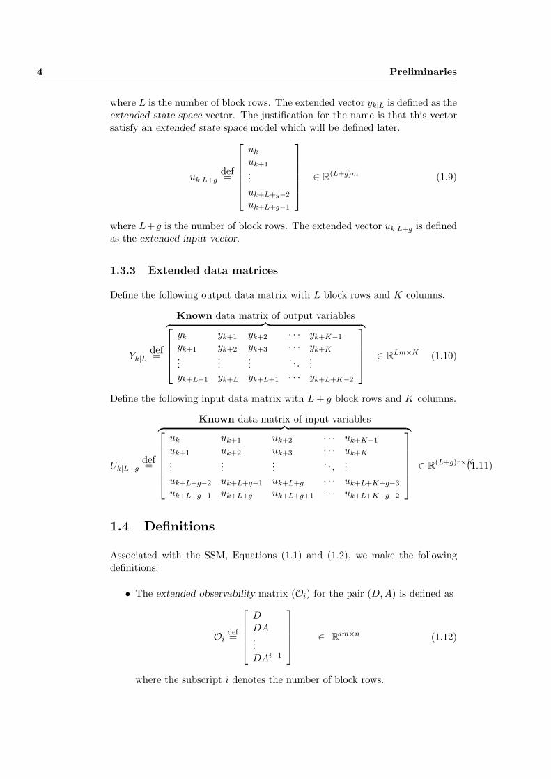
Associated with the SSM, Equations (1.1) and (1.2), we make the followingdefinitions:
• The extended observability matrix (Oi) for the pair (D,A) is defined as
Oidef=
DDA...DAi−1
∈ Rim×n (1.12)
where the subscript i denotes the number of block rows.
1.5 Extended output equation 5
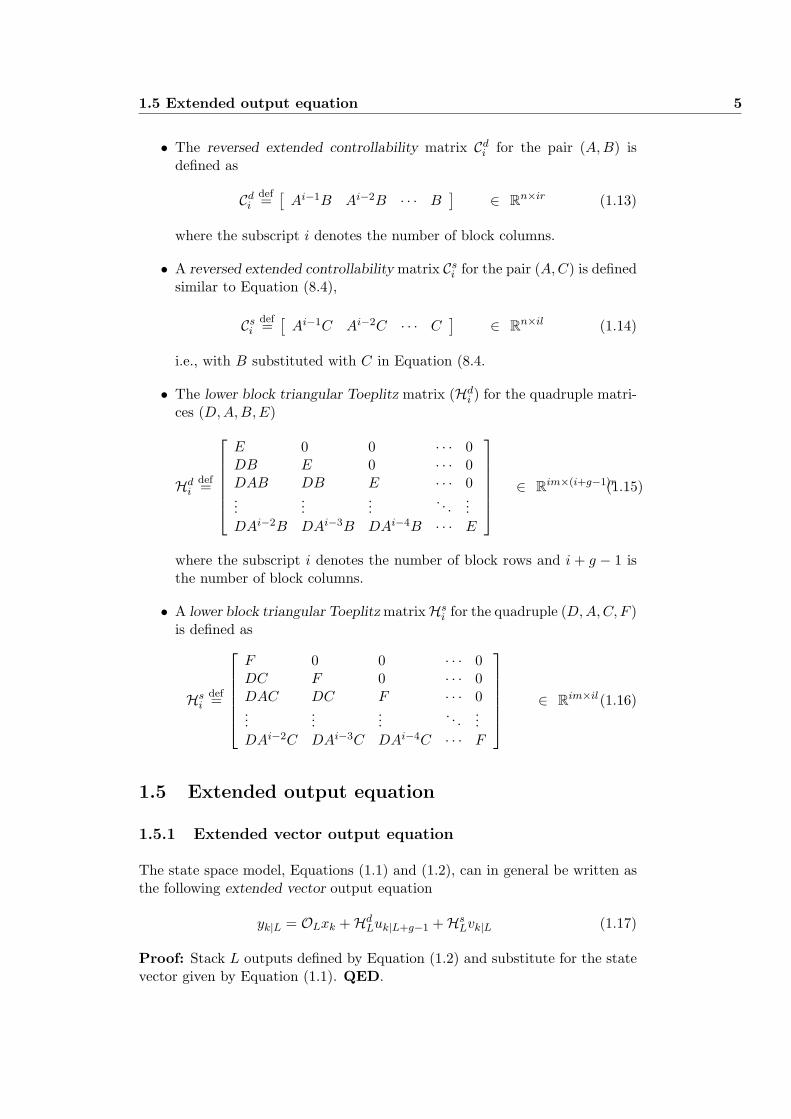
• The reversed extended controllability matrix Cdi for the pair (A,B) is
defined as
Cdi
def=[
Ai−1B Ai−2B · · · B] ∈ Rn×ir (1.13)
where the subscript i denotes the number of block columns.
• A reversed extended controllability matrix Csi for the pair (A,C) is defined
similar to Equation (8.4),
Csi
def=[
Ai−1C Ai−2C · · · C] ∈ Rn×il (1.14)
i.e., with B substituted with C in Equation (8.4.
• The lower block triangular Toeplitz matrix (Hdi ) for the quadruple matri-
ces (D, A,B,E)
Hdi
def=
E 0 0 · · · 0DB E 0 · · · 0DAB DB E · · · 0...
......
. . ....
DAi−2B DAi−3B DAi−4B · · · E
∈ Rim×(i+g−1)r(1.15)
where the subscript i denotes the number of block rows and i + g − 1 isthe number of block columns.
• A lower block triangular Toeplitz matrixHsi for the quadruple (D, A,C, F )
is defined as
Hsi
def=
F 0 0 · · · 0DC F 0 · · · 0DAC DC F · · · 0...
......
. . ....
DAi−2C DAi−3C DAi−4C · · · F
∈ Rim×il(1.16)
1.5 Extended output equation
1.5.1 Extended vector output equation
The state space model, Equations (1.1) and (1.2), can in general be written asthe following extended vector output equation
yk|L = OLxk +HdLuk|L+g−1 +Hs
Lvk|L (1.17)
Proof: Stack L outputs defined by Equation (1.2) and substitute for the statevector given by Equation (1.1). QED.
6 Preliminaries
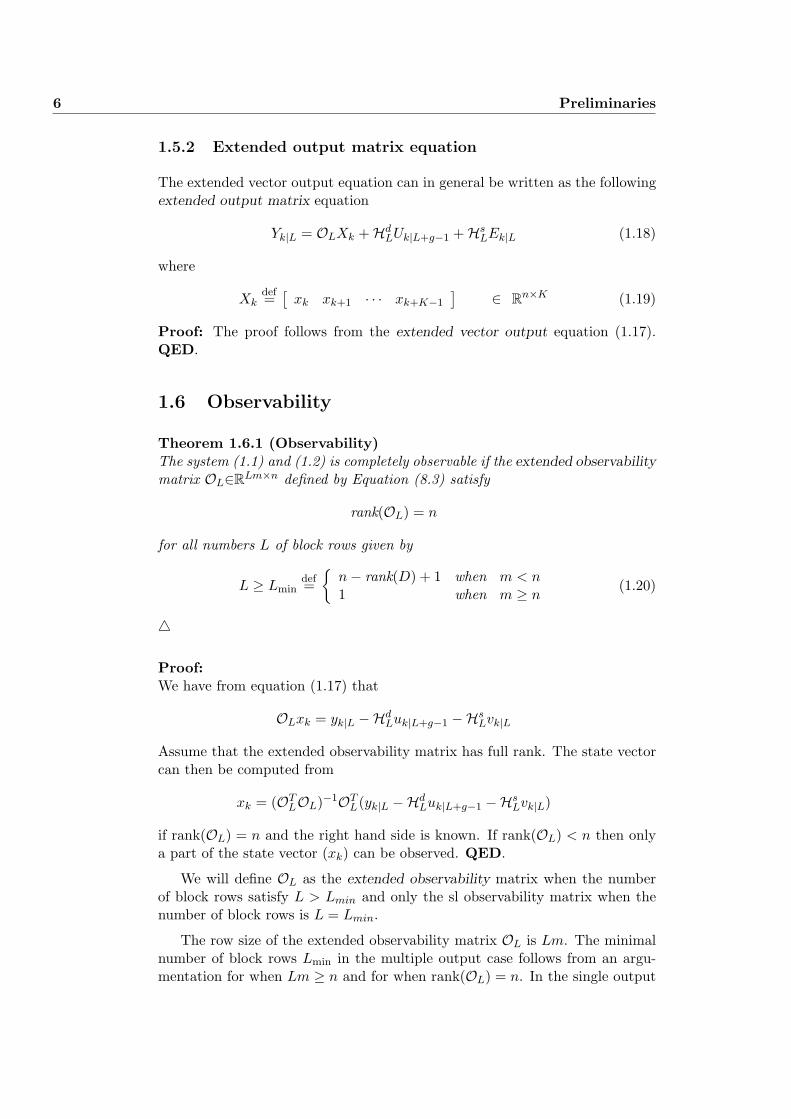
1.5.2 Extended output matrix equation
The extended vector output equation can in general be written as the followingextended output matrix equation
Yk|L = OLXk +HdLUk|L+g−1 +Hs
LEk|L (1.18)
where
Xkdef=
[xk xk+1 · · · xk+K−1
] ∈ Rn×K (1.19)
Proof: The proof follows from the extended vector output equation (1.17).QED.
1.6 Observability
Theorem 1.6.1 (Observability)The system (1.1) and (1.2) is completely observable if the extended observabilitymatrix OL∈RLm×n defined by Equation (8.3) satisfy
rank(OL) = n
for all numbers L of block rows given by
L ≥ Lmindef=
{n− rank(D) + 1 when m < n1 when m ≥ n
(1.20)
4
Proof:We have from equation (1.17) that
OLxk = yk|L −HdLuk|L+g−1 −Hs
Lvk|L
Assume that the extended observability matrix has full rank. The state vectorcan then be computed from
xk = (OTLOL)−1OT
L(yk|L −HdLuk|L+g−1 −Hs
Lvk|L)
if rank(OL) = n and the right hand side is known. If rank(OL) < n then onlya part of the state vector (xk) can be observed. QED.
We will define OL as the extended observability matrix when the numberof block rows satisfy L > Lmin and only the sl observability matrix when thenumber of block rows is L = Lmin.
The row size of the extended observability matrix OL is Lm. The minimalnumber of block rows Lmin in the multiple output case follows from an argu-mentation for when Lm ≥ n and for when rank(OL) = n. In the single output
1.6 Observability 7
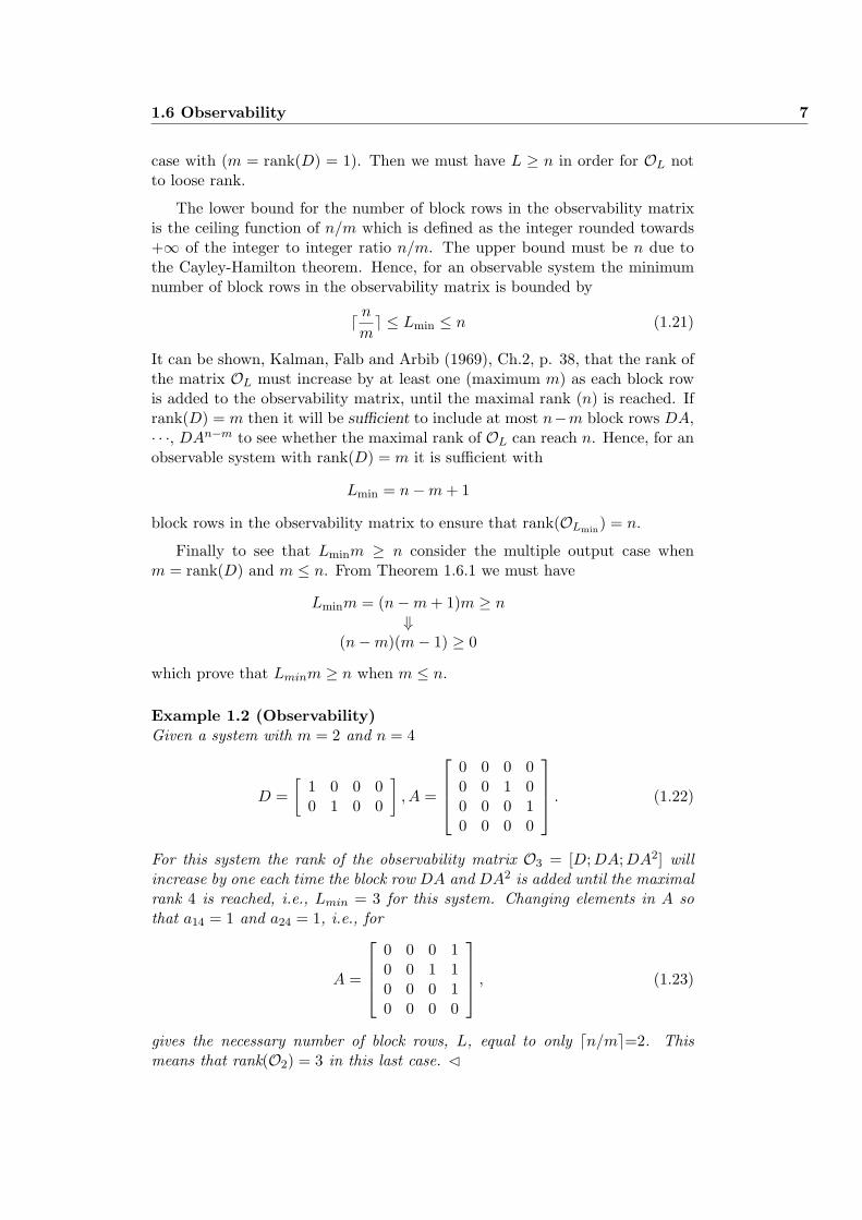
case with (m = rank(D) = 1). Then we must have L ≥ n in order for OL notto loose rank.
The lower bound for the number of block rows in the observability matrixis the ceiling function of n/m which is defined as the integer rounded towards+∞ of the integer to integer ratio n/m. The upper bound must be n due tothe Cayley-Hamilton theorem. Hence, for an observable system the minimumnumber of block rows in the observability matrix is bounded by
d n
me ≤ Lmin ≤ n (1.21)
It can be shown, Kalman, Falb and Arbib (1969), Ch.2, p. 38, that the rank ofthe matrix OL must increase by at least one (maximum m) as each block rowis added to the observability matrix, until the maximal rank (n) is reached. Ifrank(D) = m then it will be sufficient to include at most n−m block rows DA,· · ·, DAn−m to see whether the maximal rank of OL can reach n. Hence, for anobservable system with rank(D) = m it is sufficient with
Lmin = n−m + 1
block rows in the observability matrix to ensure that rank(OLmin) = n.
Finally to see that Lminm ≥ n consider the multiple output case whenm = rank(D) and m ≤ n. From Theorem 1.6.1 we must have
Lminm = (n−m + 1)m ≥ n⇓
(n−m)(m− 1) ≥ 0
which prove that Lminm ≥ n when m ≤ n.
Example 1.2 (Observability)Given a system with m = 2 and n = 4
D =[
1 0 0 00 1 0 0
], A =
0 0 0 00 0 1 00 0 0 10 0 0 0
. (1.22)
For this system the rank of the observability matrix O3 = [D;DA;DA2] willincrease by one each time the block row DA and DA2 is added until the maximalrank 4 is reached, i.e., Lmin = 3 for this system. Changing elements in A sothat a14 = 1 and a24 = 1, i.e., for
A =
0 0 0 10 0 1 10 0 0 10 0 0 0
, (1.23)
gives the necessary number of block rows, L, equal to only dn/me=2. Thismeans that rank(O2) = 3 in this last case. ¢
8 Preliminaries
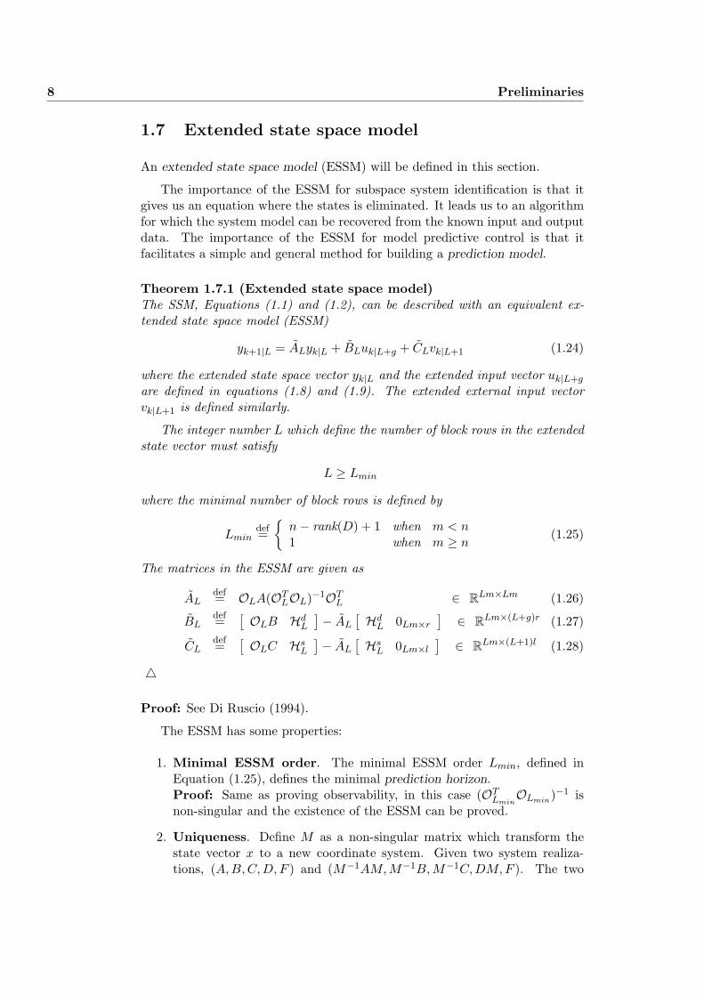
1.7 Extended state space model
An extended state space model (ESSM) will be defined in this section.
The importance of the ESSM for subspace system identification is that itgives us an equation where the states is eliminated. It leads us to an algorithmfor which the system model can be recovered from the known input and outputdata. The importance of the ESSM for model predictive control is that itfacilitates a simple and general method for building a prediction model.
Theorem 1.7.1 (Extended state space model)The SSM, Equations (1.1) and (1.2), can be described with an equivalent ex-tended state space model (ESSM)
yk+1|L = ALyk|L + BLuk|L+g + CLvk|L+1 (1.24)
where the extended state space vector yk|L and the extended input vector uk|L+g
are defined in equations (1.8) and (1.9). The extended external input vectorvk|L+1 is defined similarly.
The integer number L which define the number of block rows in the extendedstate vector must satisfy
L ≥ Lmin
where the minimal number of block rows is defined by
Lmindef=
{n− rank(D) + 1 when m < n1 when m ≥ n
(1.25)
The matrices in the ESSM are given as
ALdef= OLA(OT
LOL)−1OTL ∈ RLm×Lm (1.26)
BLdef=
[ OLB HdL
]− AL
[ HdL 0Lm×r
] ∈ RLm×(L+g)r (1.27)
CLdef=
[ OLC HsL
]− AL
[ HsL 0Lm×l
] ∈ RLm×(L+1)l (1.28)
4
Proof: See Di Ruscio (1994).
The ESSM has some properties:
1. Minimal ESSM order. The minimal ESSM order Lmin, defined inEquation (1.25), defines the minimal prediction horizon.Proof: Same as proving observability, in this case (OT
LminOLmin)−1 is
non-singular and the existence of the ESSM can be proved.
2. Uniqueness. Define M as a non-singular matrix which transform thestate vector x to a new coordinate system. Given two system realiza-tions, (A,B, C,D, F ) and (M−1AM,M−1B, M−1C, DM,F ). The two
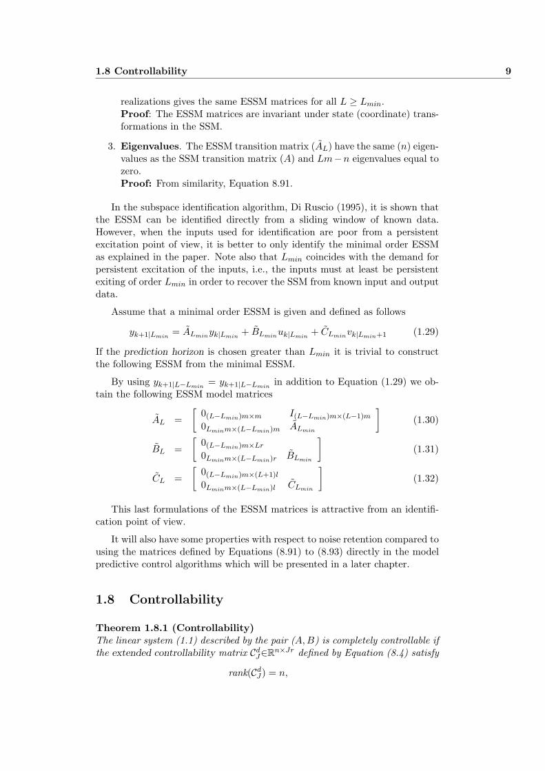
1.8 Controllability 9
realizations gives the same ESSM matrices for all L ≥ Lmin.Proof: The ESSM matrices are invariant under state (coordinate) trans-formations in the SSM.
3. Eigenvalues. The ESSM transition matrix (AL) have the same (n) eigen-values as the SSM transition matrix (A) and Lm−n eigenvalues equal tozero.Proof: From similarity, Equation 8.91.
In the subspace identification algorithm, Di Ruscio (1995), it is shown thatthe ESSM can be identified directly from a sliding window of known data.However, when the inputs used for identification are poor from a persistentexcitation point of view, it is better to only identify the minimal order ESSMas explained in the paper. Note also that Lmin coincides with the demand forpersistent excitation of the inputs, i.e., the inputs must at least be persistentexiting of order Lmin in order to recover the SSM from known input and outputdata.
Assume that a minimal order ESSM is given and defined as follows
yk+1|Lmin= ALminyk|Lmin
+ BLminuk|Lmin+ CLminvk|Lmin+1 (1.29)
If the prediction horizon is chosen greater than Lmin it is trivial to constructthe following ESSM from the minimal ESSM.
By using yk+1|L−Lmin= yk+1|L−Lmin
in addition to Equation (1.29) we ob-tain the following ESSM model matrices
AL =[
0(L−Lmin)m×m I(L−Lmin)m×(L−1)m
0Lminm×(L−Lmin)m ALmin
](1.30)
BL =[
0(L−Lmin)m×Lr
0Lminm×(L−Lmin)r BLmin
](1.31)
CL =[
0(L−Lmin)m×(L+1)l
0Lminm×(L−Lmin)l CLmin
](1.32)
This last formulations of the ESSM matrices is attractive from an identifi-cation point of view.
It will also have some properties with respect to noise retention compared tousing the matrices defined by Equations (8.91) to (8.93) directly in the modelpredictive control algorithms which will be presented in a later chapter.
1.8 Controllability
Theorem 1.8.1 (Controllability)The linear system (1.1) described by the pair (A,B) is completely controllable ifthe extended controllability matrix Cd
J∈Rn×Jr defined by Equation (8.4) satisfy
rank(CdJ) = n,
10 Preliminaries
for all numbers, J , of block rows given by
J ≥ Jmindef=
{n− rank(B) + 1 when r < n,1 when r ≥ n.
(1.33)
4
1.9 ARMAX and extended state space model
Given a polynomial (ARMAX) model in the discrete time domain as follows
yk+L|1 = A1yk|L + B1uk|L+g + C1vk|L+1 (1.34)
where the polynomial (ARMAX) model matrices are given by
A1def=
[A1 A2 · · · AL
] ∈ Rm×Lm,
B1def=
[B0 B1 · · · BL−1+g BL+g
] ∈ Rm×(L+g)r,
C1def=
[C0 C1 · · · CL CL+1
] ∈ Rm×(L+1)m.
(1.35)
where Ai ∈ Rm×m for i = 1, . . . , L, Bi ∈ Rm×r for i = 0, . . . , L+ g, Ci ∈ Rm×m
for i = 0, . . . , L + 1. This model can be formulated directly as an ESSM whichhave relations to the SSM matrices. We have
AL =
0 I · · · 0 00 0 · · · 0 0...
.... . . . . .
...0 0 · · · 0 IA1 A2 · · · AL−1 AL
∈ RLm×Lm (1.36)
BL =
0 0 · · · 0 0 00 0 · · · 0 0 0...
.... . . . . .
......
0 0 · · · 0 0 0B0 B1 · · · BL+g−2 BL+g−1 BL+g
∈ RLm×(L+g)r(1.37)
CL =
0 0 · · · 0 0 00 0 · · · 0 0 0...
.... . . . . .
......
0 0 · · · 0 0 0C0 C0 · · · CL−1 CL CL+1
∈ RLm×(L+1)m (1.38)
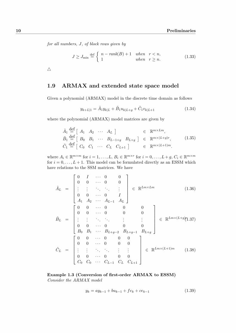
Example 1.3 (Conversion of first-order ARMAX to ESSM)Consider the ARMAX model
yk = ayk−1 + buk−1 + fek + cek−1 (1.39)
1.9 ARMAX and extended state space model 11
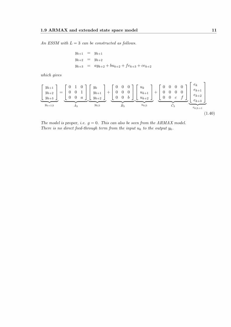
An ESSM with L = 3 can be constructed as follows.
yk+1 = yk+1
yk+2 = yk+2
yk+3 = ayk+2 + buk+2 + fek+3 + cek+2
which gives
yk+1
yk+2
yk+3
︸ ︷︷ ︸yk+1|3
=
0 1 00 0 10 0 a
︸ ︷︷ ︸A3
yk
yk+1
yk+2
︸ ︷︷ ︸yk|3
+
0 0 00 0 00 0 b
︸ ︷︷ ︸B3
uk
uk+1
uk+2
︸ ︷︷ ︸uk|3
+
0 0 0 00 0 0 00 0 c f
︸ ︷︷ ︸C3
ek
ek+1
ek+2
ek+3
︸ ︷︷ ︸ek|L+1
(1.40)
The model is proper, i.e. g = 0. This can also be seen from the ARMAX model.There is no direct feed-through term from the input uk to the output yk.

12 Preliminaries
Chapter 2
Realization theory
2.1 Introduction
A method for the realization of linear state space models from known systeminput and output time series is studied. The input-output time series are usuallyobtained from a number of independently input experiments to the system.
2.2 Deterministic case
2.2.1 Model structure and problem description
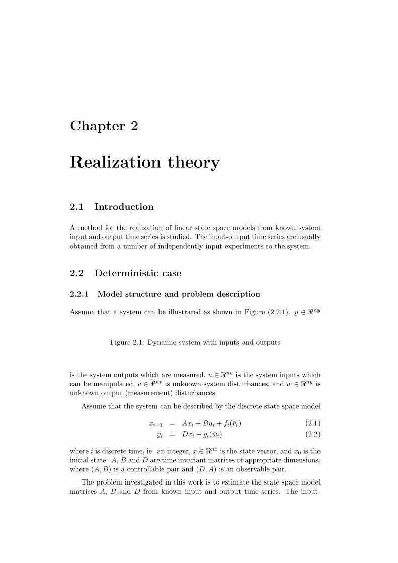
Assume that a system can be illustrated as shown in Figure (2.2.1). y ∈ <ny
Figure 2.1: Dynamic system with inputs and outputs
is the system outputs which are measured, u ∈ <nu is the system inputs whichcan be manipulated, v ∈ <nv is unknown system disturbances, and w ∈ <ny isunknown output (measurement) disturbances.
Assume that the system can be described by the discrete state space model
xi+1 = Axi + Bui + fi(vi) (2.1)yi = Dxi + gi(wi) (2.2)
where i is discrete time, ie. an integer, x ∈ <nx is the state vector, and x0 is theinitial state. A, B and D are time invariant matrices of appropriate dimensions,where (A,B) is a controllable pair and (D, A) is an observable pair.
The problem investigated in this work is to estimate the state space modelmatrices A, B and D from known input and output time series. The input-
14 Realization theory
output time series are usually obtained from a number of independently inputexperiments to the system. f(·) and g(·) are non-linear functions.
The derivation of the method will be based on the assumption that thefunctions f and g are linear, ie.
fi(vi) = Cvi gi(wi) = wi (2.3)
This is not a restriction, but a choice, which make it possible to apply stochasticrealization theory to estimate the noise covariance matrices, in addition to A,B and D.
2.2.2 Impulse response model
A linear state space model xx+1 = Axk + Buk and yk = Dxk + Euk with theinitial state x0 given, can be described as the following impulse response model
yk = DAkx0 +k∑
i=1
DAk−iBui−1 + Euk. (2.4)
We define the matrix
Hk−i+1 = DAk−iB ∈ Rny×nu, (2.5)
as the impulse response matrix at time instant k− i+1. hence, the output, yk,at time instant k is defined in terms of the impulse response matrices H1 = DB,H2 = DAB, . . ., Hk = DAk−1B.
2.2.3 Determination of impulse responses
To determine the impulse responses a set of process experiments have to beperformed. uj
i is defined as the control input at time instant i for experimentnumber j, and yj
i is the corresponding process output. The derivation is basedon information from mk = nu+1 experiments, however, this is not a restriction.
The derivation is based on the assumption that the noise vectors f and gare the same for each experiment. In this case, exact impulse responses are theresult of this method.
In most cases, the noise vectors are different for each experiment, for exam-ple when the disturbances are white noise. In this case errors are introduced,and a crude estimate may occur. However, these errors may be reduced.
Time instant i = 1
x1 = Ax0 + Cv0 + Bu0 (2.6)y1 = D(Ax0 + Cv0) + w1 + DBu0 (2.7)
2.2 Deterministic case 15
or in matrix form
y1 =[
z1 H1
] [1u0
](2.8)
where
H1 = DB (2.9)z1 = D(Ax0 + Cv0) + w1 (2.10)
For nu + 1 experiments
Y1 =[
z1 H1
] [ones(1, nu + 1)
U0
](2.11)
where
Y1 =[
y11 y2
1 · · · ynu+11
]U0 =
[u1
0 u20 · · · unu+1
0
](2.12)
Time instant i = 2
x2 = A(Ax0 + Cv0) + Cv1 + ABu0 + Bu1 (2.13)y2 = D(A2x0 + ACv0 + Cv1) + w2 + DABu0 + DBu1 (2.14)
or in matrix form
y2 =[
z2 H2 H1
]
1u0
u1
(2.15)
where
H2 = DAB (2.16)z2 = D(A2x0 + ACv0 + Cv1) + w2 (2.17)
For nu + 1 experiments
Y2 =[
z2 H2 H1
]
ones(1, nu + 1)U0
U1
(2.18)
where
Y2 =[
y12 y2
2 · · · ynu+12
]U1 =
[u1
1 u21 · · · unu+1
1
](2.19)
Time instants i = 1, ..., 2nThe results, for time instants 1 to 2n, may be stacked in the following matrix
16 Realization theory
system, which have a suitable structure for the determination of the unknownmatrices Hi and the vectors zi. Note that the information from time instanti = 0 is not necessary at this point.
Y1
Y2
Y3...
Y2n
=
z1 H1 0 0 · · · 0z2 H2 H1 0 0z3 H3 H2 H1 · · · 0...
.... . . . . . . . .
...z2n H2n · · · H3 H2 H1
ones(1, nu + 1)U0
U1
U2...
U2n−1
(2.20)
This linear matrix equation may be solved recursively. Start with i = 1 andsolve for [z1 H1]. Then successively solve the i th equation for [zi Hi] fori = 1, ..., 2n. We have
[zi Hi
] [ones(1, nu + 1)
U0
]= (Yi −
i−1∑
k=1
Hi−kUk) (2.21)
or
[zi Hi
]= (Yi −
i−1∑
k=1
Hi−kUk)[
ones(1, nu + 1)U0
]−1
(2.22)
because the matrix is non singular by the definition of the input experimentsuj j = 1, ..., nu + 1.
We have now determined the impulse responses Hi and the vectors zi forall i = 1, ..., 2n which contain information of noise and initial values. Hi and zi
can be expressed by
Hi = DAi−1B (2.23)
zi = DAix0 +i∑
k=1
DAi−kCvk−1 + wi (2.24)
Observe that the sequence zi ∀ i = 1, ..., 2n is generated by the following statespace model.
si+1 = Asi + Cvi s0 = x0 (2.25)zi = Dsi + wi (2.26)
where for the moment, z0, is undefined. Define e = x− s, then
ei+1 = Aei + Bui e0 = 0 (2.27)yi = Dei + zi (2.28)
The problem is now reduced to estimate the matrices (A,B, D), which satisfythe model, Equations (2.27) and (2.28), from known impulse respenses Hi. Inaddition, initial values and noise statistics can be estimated from the model
2.2 Deterministic case 17
given by Equations (2.25) and (2.26) where zi and the matrices A, and D areknown.
z0 must be defined before continuing. At time instant i = 0 we have y0 =Dx0 + w0. For nu + 1 experiments
Y0 = Z0 (2.29)Y0 =
[y10 y2
0 · · · ynu+10
]Z0 =
[z10 z2
0 · · · znu+10
](2.30)
We have assumed that the initial values are equal for all experiments. In thiscase z0 is chosen as one of the columns in Y0. z0 can even be computed from
[z0 0
]= Y0
[ones(1, nu + 1)
U0
]−1
(2.31)
However, this last method can have numerical disadvantages. It is a methodfor constructing a right inverse for ones(1, nu+1), and is nothing but the meanof the columns of the matrix Y0.
If the initial values are different for some or all nu + 1 experiments, then,there are obviously many choices for z0. One choice is the mean of the columnsof the matrix Y0, which is consistent with the case of equal initial values, ie.
z0 =1
nu + 1
nu+1∑
j=1
yj0 (2.32)
2.2.4 Redundant or missing information
Assume that the number of experiments, m, are different from nu + 1. In thiscase we have
[zi Hi
]U0 = (Yi −
i−1∑
k=1
Hi−kUk) (2.33)
Assume that m ≥ nu+1 and rank(U0UT0 ) = m, then, the solution of Equation
(2.33) with respect to Hi and zi is given by
[zi Hi
]= (Yi −
i−1∑
k=1
Hi−kUk)UT0 (U0U
T0 )−1 (2.34)
Assume that m < nu + 1 or rank(U0UT0 ) < m. An approximate solution is
determined by
[zi Hi
]= (Yi −
i−1∑
k=1
Hi−kUk)V S+UT (2.35)
where
U0 = U SV T (2.36)
18 Realization theory
is the singular value decomposition. In any cases the solutions discussed aboveminimizes the 2 - norm of the error residual.
Note the connection to the theory of multivariate calibration, Martens andNæss (1989), where usually a steady state model of the form y = Hu + z ischosen to fit the data. The gain H is computed in the same way as outlinedabove. Our method can thus be viewed as a dynamic extension of the theoryof multivariate calibration.
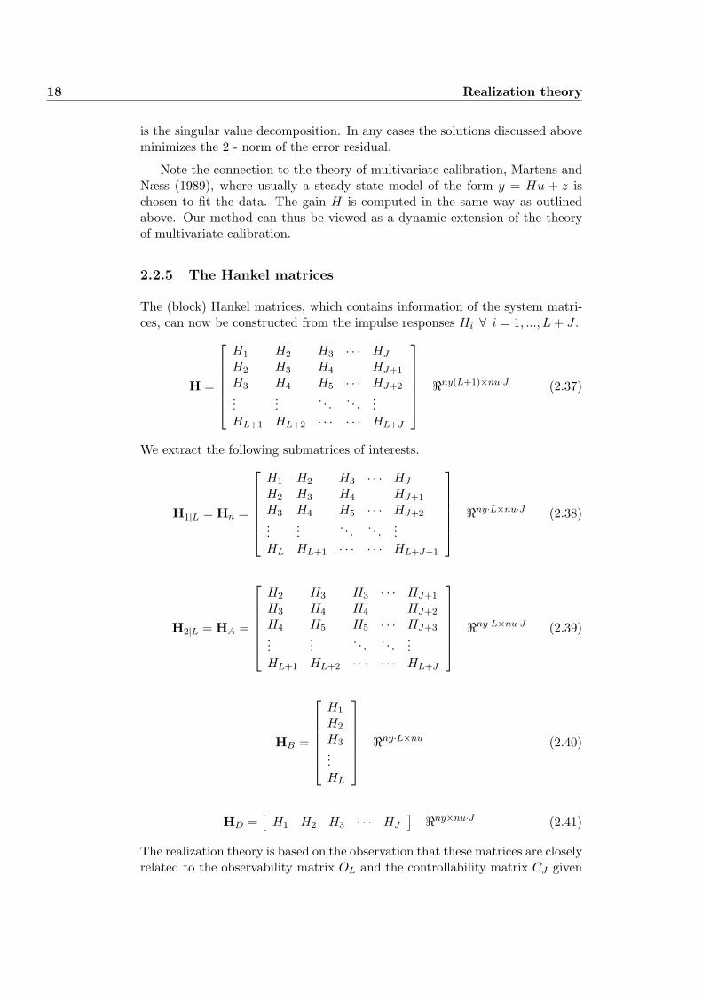
2.2.5 The Hankel matrices
The (block) Hankel matrices, which contains information of the system matri-ces, can now be constructed from the impulse responses Hi ∀ i = 1, ..., L + J .
H =
H1 H2 H3 · · · HJ
H2 H3 H4 HJ+1
H3 H4 H5 · · · HJ+2...
.... . . . . .
...HL+1 HL+2 · · · · · · HL+J
<ny(L+1)×nu·J (2.37)
We extract the following submatrices of interests.
H1|L = Hn =
H1 H2 H3 · · · HJ
H2 H3 H4 HJ+1
H3 H4 H5 · · · HJ+2...
.... . . . . .
...HL HL+1 · · · · · · HL+J−1
<ny·L×nu·J (2.38)
H2|L = HA =
H2 H3 H3 · · · HJ+1
H3 H4 H4 HJ+2
H4 H5 H5 · · · HJ+3...
.... . . . . .
...HL+1 HL+2 · · · · · · HL+J
<ny·L×nu·J (2.39)
HB =
H1
H2
H3...HL
<ny·L×nu (2.40)
HD =[
H1 H2 H3 · · · HJ
] <ny×nu·J (2.41)
The realization theory is based on the observation that these matrices are closelyrelated to the observability matrix OL and the controllability matrix CJ given
2.2 Deterministic case 19
by.
OL =
DDADA2
...DAL−1
<ny·L×nx (2.42)
CJ =[
B AB A2B · · · AJ−1B] <nx×nu·J (2.43)
The following factorization is the basic for the realization of the number ofstates nx and the system matrices A, B and D.
Hn = H1|L = OLCJ (2.44)
At this stage it must be pointed out that the factorization of the Hankel ma-trix by numerical methods, usually results in observability and controllabilitymatrices for a model representation in a different co-ordinate system than theunderlying system.
The number of states nx is estimated as the rank of Hn = H1|L. To obtaina proper estimate we must ensure that
L ≥ nx− rank(D) + 1, J ≥ nx− rank(B) + 1. (2.45)
The reason for this is that, in this case, rank(OL) = nx when the pair (D, A) isobservable, and similarly, rank(CJ) = nx when the pair (A,B) is controllable.OL and CJ may be determined by a suitable factorization of the known blockHankel matrix, Hn = H1|L. The system matrices is then chosen to satisfy thefollowing three matrix relations.
H1|L = HA = OLACJ , HB = OLB, HD = DCJ (2.46)
The system matrices are then estimated by
A = (OTLOL)−1OT
LHACTJ (CJCT
J )−1, (2.47)B = (OT
LOL)−1OTLHB, (2.48)
D = HDCTJ (CJCT
J )−1. (2.49)
Assume for the moment that v = w = 0. The initial values satisfy, in this case
zn = OLAx0 (2.50)
and can be estimated by
x0 = A−1(OTLO)−1OT
Lzn (2.51)
if A is non-singular. If A is singular then the information from time instanti = 0, y0 = Dx0 + w0, or z0 = y0 = Dx0 by assumption, can be added to thealgorithm to avoid the inversion. We have
x0 = (OTLOL)−1OT
L zn (2.52)
20 Realization theory
where zn = [zT0 , zT
n−1]T is the vector where z0 is augmented to the first n − 1
elements in zn.
Note that the estimated model matrices usually are related to a different co-ordinate system than the underlying model. Let x = T x be the transformationfrom the estimated state vector x to the underlying state vector x. The observ-ability and controllability matrices are given by OL = OLT and CJ = T−1CJ .Which means that the transformation T is given by
T = (OTLOL)−1OT
LOL, T−1 = CJCTJ (CJCT
J )−1. (2.53)
2.2.6 Balanced and normalized realizations
Perform the singular value decomposition, SVD, of the finite block Hankel ma-trix Hn.
H1|L = Hn = OLCJ = USV T = US1S2VT . (2.54)
The order of the state space model is equal to the number of the non zerosingular values which is the same as the rank of Hn, ie. nx = rank(Hn).A reduced model is directly determined by choosing a subset of the non zerosingular values.
The following choices for the factorization of the Hankel matrix into theproduct of the observability and controllability matrices results directly fromthe SVD.
OL = US1, CJ = S2VT (internally balanced),
OL = U, CJ = SV T (output normal),OL = US, CJ = V T (input normal).
(2.55)
These factorizations are called internally balanced, output normal and inputnormal, respectively, according to the definitions by Moore (1981). See alsoSilverman and Bettayeb (1980). The meaning of these definitions will be madeclear later in this section.
If the internally balanced realization, as in Aoki (1990), is used, then thesystem matrices are estimated by
A = S−T1 UTHAV S−T
2
B = S−T1 UTHB
D = HDV S−T2
(internally balanced) (2.56)
The output normal and input normal realizations are related to the co-ordinatesystem, in which the internally balanced system is presented, by a transforma-tion. These realizations are shown below for completeness.
A = UTHAV S−1
B = UTHB
D = HDV S−1
(output normal) (2.57)
2.2 Deterministic case 21
A = S−1UTHAVB = S−1UTHB
D = HDV
(input normal) (2.58)
The initial values may in all cases be estimated from Equation (2.51) if v =w = 0.
Note that the matrix multiplications to perform B and D are not necessary,because B is equal to the first nx x nu submatrix of CJ = US1 and D isequal to the first ny x nx submatrix of OL = S2V
T , in the internally balancedrealization.
Note that the SVD is not unique, in the sense that it may exist otherorthogonal matrices U and V satisfying Hn = USV T . One can always changesign for one column in U and in the corresponding column in V . However, Sis of course unique, if the singular values are ordered in descending order ofmagnitude along the diagonal. This means that the estimated system matricesare not unique, because the estimated matrices are dependent on the choice ofU and V , this is contradictory to the statement of uniqueness in Aoki (1990)pp. 109.
However, the estimates have the properties that the L - observability andthe J - controllability grammians defined by
Wo,L = OTLOL =
L∑
i=1
A(i−1)T DT DA(i−1) (2.59)
Wc,J = CJCTJ =
J∑
i=1
A(i−1)BBT A(i−1)T (2.60)
satisfy
Wo,L = Snx Wc,J = Snx (internally balanced)Wo,L = I Wc,J = S2
nx (output normal)Wo,L = S2
nx Wc,J = I (input normal)(2.61)
This can be shown by substituting the L - observability and the J - controlla-bility matrices given in (2.55) into the grammians, Equations (2.59) and (2.60).
A model which satisfy one of the properties in (2.61) is called internallybalanced, output normal or input normal, respectively. This definitions are dueto Moore (1981).
The model produced by the method of Aoki (1990) is by this definition in-ternally balanced. A model is called internally balanced if the correspondingobservability and controllability grammians are equal to the same diagonal ma-trix. Particularly, a diagonal matrix with the non zero singular values of theHankel matrix on the diagonal, in this case. This imply that the new system is”as controllable as it is observable”.
Note that the estimates (2.56) are not internally balanced due to the infiniteobservability and the infinite controllability grammians Wo and Wc, which are
22 Realization theory
the grammians for a stable system when n →∞ in Equations (2.59) and (2.60).These grammians satisfy the discrete Lyapunov matrix equations
AT WoA−Wo = −DT D, (2.62)AWcA
T −Wc = −BBT , (2.63)
if A is stable.
The estimate of the process model is usually obtained from finite Hankelmatrices, i.e., for finite L and J . Note also that usually L = J . This modelestimate may be transformed to a model representation with balanced or nor-malized grammians which satisfy the Lyapunov equations (2.62) and (2.63).See Moore (1981), Silverman and Bettayeb (1980) and Laub (1980) for thedetermination of such a transformation.
The statement that the internally balanced estimates are not unique willnow be clarified. Suppose that the model (A,B, D) is transformed to a newco-ordinate system with x = T x. The grammians for the new system is thengiven by
Wo = T T WoT, (2.64)Wc = T−1WcT
−T . (2.65)
Assume that both realizations is internally balanced so that
T T WoT = T−1WcT−T = Snx, (2.66)
Wo = Wc = Snx. (2.67)
This implies that
T−1S2nxT = S2
nx, (2.68)(2.69)
which constrain T to be a diagonal matrix with ±1 in each diagonal entry. Theargumentation shows that a model which is internally balanced is not unique.However, the set of such models are constrained within sign changes.
2.2.7 Error analysis
When the order of the state space model is chosen less than the rank of theHankel matrix, errors is introduced.
The output sequence may be written as
yi =i∑
k=1
Hi−kuk−1 + zi (2.70)
where the impulse responses Hi and the noise terms zi are known. See Section(2.2.3).
2.3 Numerical examples 23
The estimated state space model can be written in input output form as
yi =i∑
k=1
Hi−kuk−1 + zi (2.71)
where Hi are the impulse responses computed from the estimated state spacemodel, and zi is the output from an estimated model of the noise and initialvalues based on the computed sequence zi.
The estimation error is given by
εi =i∑
k=1
∆Hi−kuk−1 + ∆zi (2.72)
where ∆zi = zi + zi, which states that the output sequence can be written
yi = yi + εi (2.73)
2.3 Numerical examples
2.3.1 Example 1
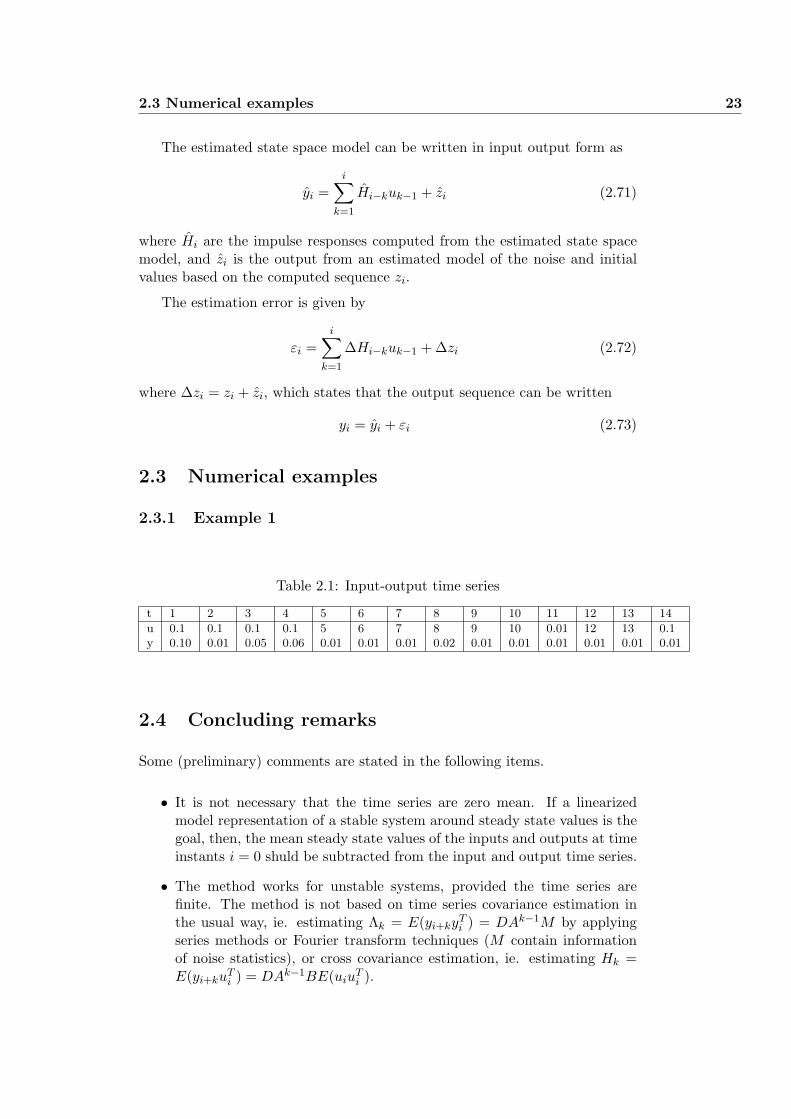
Table 2.1: Input-output time series
t 1 2 3 4 5 6 7 8 9 10 11 12 13 14
u 0.1 0.1 0.1 0.1 5 6 7 8 9 10 0.01 12 13 0.1y 0.10 0.01 0.05 0.06 0.01 0.01 0.01 0.02 0.01 0.01 0.01 0.01 0.01 0.01
2.4 Concluding remarks
Some (preliminary) comments are stated in the following items.
• It is not necessary that the time series are zero mean. If a linearizedmodel representation of a stable system around steady state values is thegoal, then, the mean steady state values of the inputs and outputs at timeinstants i = 0 shuld be subtracted from the input and output time series.
• The method works for unstable systems, provided the time series arefinite. The method is not based on time series covariance estimation inthe usual way, ie. estimating Λk = E(yi+ky
Ti ) = DAk−1M by applying
series methods or Fourier transform techniques (M contain informationof noise statistics), or cross covariance estimation, ie. estimating Hk =E(yi+ku
Ti ) = DAk−1BE(uiu
Ti ).
24 Realization theory
• The method works for non-minimum phase systems. If the time series aregenerated from a state-output system (A, B,D), then the algorithm real-ize an equivalent state-output system (A, B, D) with respect to impulseresponses, poles and zeros, even if the system is non-minimum phase. Theco-ordinate system in which the realized model is presented, is of coursegenerally different from the underlying co-ordinate system. The Markovparameters are estimated from information of both u and y, not only y asin standard realizing algorithms such as Aokis method. Recall that trans-mission zeros cannot be observed from the outputs alone, which meansthat realizing algorithms which are based on the estimation of Markovparameters from y alone do not work for non-minimum phase systems.
• If the time series are generated from a transition-output system (A, B,D, E),an essentially equivalent state-output system (A, B, D), with respect topoles, zeros and impulse responses, is realized by this method. The in-stantaneous dynamics from u to y in the transition-output system, arerealized with eigenvalues equal to zero in A, which means that states areadded which are infinitely fast. The spectrum of A is essentially equiva-lent to the spectrum of A, exept for som zero poles added. The zeros ofthe realization (A, B, D) is generally different from the zeros of an under-lying system with realization (A,B, D, E). But the realization (A, B, D)can be changed to a realization (A, B, D, E), with the same zeros as theunderlying system (A,B, D,E). This means that if the underlying system(A,B,D, E) is non-minimum phase (zeros outside the unit-circle in thez-plane), the realization (A, B, D) can lock like a minimum phase system(zeros inside the unit-circle in the z-plane), hence; If there are zero eigen-values (or zero in a relative sense) in the realization (A, B, D), change to(A,B,D, E) system before computing zeros!
References
Aoki M. (1987). State Space Modeling of Time Series. Springer-Verlag Berlin,Heidelberg.
Aoki M. (1990). State Space Modeling of Time Series. Springer-Verlag Berlin,Heidelberg.
Laub, A. J. (1980). Computation of ”balancing” transformations. Proc.JACC, San Francisco, FA8-E.
Martens, H. and T. Næss (1989). ”Multivariate Calibration”. John Wiley andSons Ltd. Chichester.
Moore, B. C. (1981). Principal Component Analysis in Linear Systems: Con-trollability, Observability, and Model Reduction. IEEE Trans. on Auto-matic Control, Vol. AC-26, pp. 17-31.

2.4 Concluding remarks 25
Silverman L. M. and M. Bettayeb (1980). Optimal approximation of linearsystems. Proc. JACC, San Francisco, FA8-A.

26 Realization theory
Chapter 3
Combined Deterministic andStochastic SystemIdentification and Realization- DSR: A subspace approachbased on observations 1
Abstract
The paper presentes a numerically stable and general algorithm for identifica-tion and realization of a complete dynamic linear state space model, includingthe system order, for combined deterministic and stochastic systems from timeseries. A special property of this algorithm is that the innovations covariancematrix and the Markov parameters for the stochastic sub-system are determineddirectly from a projection of known data matrices, without e.g. recursions ofnon-linear matrix Riccatti equations. A realization of the Kalman filter gainmatrix is determined from the estimated extended observability matrix and theMarkov parameters. Monte Carlo simulations are used to analyze the statisticalproperties of the algorithm as well as to compare with existing algorithms.
1ECC95 paper extended with proofs, new results and theoretical comparison with existingsubspace identification methods. Also in Computer Aided Time Series Modeling, Edited byMasanao Aoki, Springer Verlag, 1997.
28 Subspace identificatio
3.1 Introduction
System identification can be defined as building mathematical models of sys-tems based on observed data. Traditionally a set of model structures with somefree parameters are specified and a prediction error (PE) criterion measuringthe difference between the observed outputs and the model outputs is optimizedwith respect to the free parameters. In general, this will result in a non linearoptimization problem in the free parameters even when a linear time invari-ant model is specified. A tremendous amount of research has been reported,resulting in the so called prediction error methods (PEM).
In our view the field of subspace identification, Larimore (1983) and (1990),Verhagen (1994), Van Overschee and De Moor (1994), Di Ruscio (1994), notonly resolves the problem of system identification but also deals with the addi-tional problem of structure identification. In subspace identification methods adata matrix is constructed from certain projections of the given system data.The observability matrix for the system is extracted as the column space of thismatrix and the system order is equal to the dimension of the column space.
Descriptions of the advantages of subspace identification methods over tra-ditional PEM can be found in Viberg (1995) and in Van Overschee (1995).
Aoki (1990) has presented a method for the realization of state space lineardiscrete time stochastic models on innovations form. See also Aoki (1994) forsome further improvements of the method. This method has many interestingnumerical properties and many of the numerical tools involved in the methodare common with the tools used by the subspace identification methods. Themethod is based on the factorization of the Hankel matrix, constructed fromcovariance matrices of the output time series, by singular value decomposition.The states are presented relative to an internally balanced coordinate system,Moore (1981), which has some interesting properties when dealing with modelreduction.
The subspace identification methods which are presented in the above refer-ences are using instrumental variables constructed from past input and outputdata in order to remove the effect of noise from future data. It should be pointedout that the method by Aoki also uses instrumental variables constructed frompast data.
The method for system identification and state space model realizationwhich is presented in this work is believed to be a valuable tool for the analysisand modeling of observed input and output data from a wide range of systems,in particular combined deterministic and stochastic dynamical systems. Onlylinear algebra is applied in order to estimate a complete linear time invariantstate space model.
Many successful applications of data based time series analysis and modelingmethods are reported. One industrial application is presented in Di Ruscio andHolmberg (1996). One particularly important application is the estimation ofeconometric models, see Aoki (1990).
3.2 Preliminary Definitions 29
The remainder of the paper is organized as follows. Section 3.2 gives a def-inition of the system and the problem considered in this work. In Section 3.3the data is organized into data matrices which satisfy an extended state spacemodel or matrix equation. Section 3.4 shows how the system order and themodel matrices can be extracted from the known data matrices. A numericallystable and efficient implementation is presented in Section 3.5. Section 3.6 givesa comparison of the method presented in this work with other published meth-ods. Real world numerical examples and theoretical Monte Carlo simulationsare presented in Section 3.7 and some concluding remarks follow in Section 3.8.
3.2 Preliminary Definitions
3.2.1 System Definition
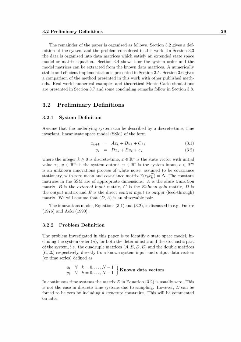
Assume that the underlying system can be described by a discrete-time, timeinvariant, linear state space model (SSM) of the form
xk+1 = Axk + Buk + Cek (3.1)yk = Dxk + Euk + ek (3.2)
where the integer k ≥ 0 is discrete-time, x ∈ Rn is the state vector with initialvalue x0, y ∈ Rm is the system output, u ∈ Rr is the system input, e ∈ Rm
is an unknown innovations process of white noise, assumed to be covariancestationary, with zero mean and covariance matrix E(eke
Tk ) = ∆. The constant
matrices in the SSM are of appropriate dimensions. A is the state transitionmatrix, B is the external input matrix, C is the Kalman gain matrix, D isthe output matrix and E is the direct control input to output (feed-through)matrix. We will assume that (D, A) is an observable pair.
The innovations model, Equations (3.1) and (3.2), is discussed in e.g. Faurre(1976) and Aoki (1990).
3.2.2 Problem Definition
The problem investigated in this paper is to identify a state space model, in-cluding the system order (n), for both the deterministic and the stochastic partof the system, i.e. the quadruple matrices (A,B, D,E) and the double matrices(C, ∆) respectively, directly from known system input and output data vectors(or time series) defined as
uk ∀ k = 0, . . . , N − 1yk ∀ k = 0, . . . , N − 1
}Known data vectors
In continuous time systems the matrix E in Equation (3.2) is usually zero. Thisis not the case in discrete time systems due to sampling. However, E can beforced to be zero by including a structure constraint. This will be commentedon later.
30 Subspace identificatio
3.2.3 Matrix Definitions
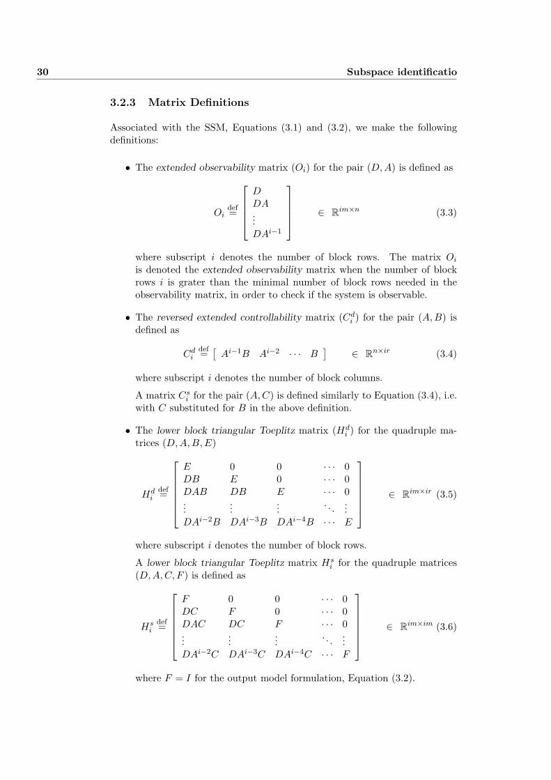
Associated with the SSM, Equations (3.1) and (3.2), we make the followingdefinitions:
• The extended observability matrix (Oi) for the pair (D, A) is defined as
Oidef=
DDA...DAi−1
∈ Rim×n (3.3)
where subscript i denotes the number of block rows. The matrix Oi
is denoted the extended observability matrix when the number of blockrows i is grater than the minimal number of block rows needed in theobservability matrix, in order to check if the system is observable.
• The reversed extended controllability matrix (Cdi ) for the pair (A,B) is
defined as
Cdi
def=[
Ai−1B Ai−2 · · · B] ∈ Rn×ir (3.4)
where subscript i denotes the number of block columns.
A matrix Csi for the pair (A,C) is defined similarly to Equation (3.4), i.e.
with C substituted for B in the above definition.
• The lower block triangular Toeplitz matrix (Hdi ) for the quadruple ma-
trices (D, A,B, E)
Hdi
def=
E 0 0 · · · 0DB E 0 · · · 0DAB DB E · · · 0...
......
. . ....
DAi−2B DAi−3B DAi−4B · · · E
∈ Rim×ir (3.5)
where subscript i denotes the number of block rows.
A lower block triangular Toeplitz matrix Hsi for the quadruple matrices
(D,A, C, F ) is defined as
Hsi
def=
F 0 0 · · · 0DC F 0 · · · 0DAC DC F · · · 0...
......
. . ....
DAi−2C DAi−3C DAi−4C · · · F
∈ Rim×im (3.6)
where F = I for the output model formulation, Equation (3.2).

3.3 Extended State Space Model 31
3.2.4 Notation
The projection A/B of two matrices A and B is defined as ABT (BBT )†B where† denotes the Moore-Penrose pseudo-inverse of a matrix.
3.3 Extended State Space Model
The state space model, Equations (3.1) and (3.2), can generally be written asthe following extended state space model (ESSM) (Di Ruscio (1994))
Yk+1|L = AYk|L + BUk|L+1 + CEk|L+1 (3.7)
where the known output and input data matrices Yk|L and Uk|L+1 are definedas follows
Yk|Ldef=
yk yk+1 yk+2 · · · yk+K−1
yk+1 yk+2 yk+3 · · · yk+K...
......
. . ....
yk+L−1 yk+L yk+L+1 · · · yk+L+K−2
∈ RLm×K (3.8)
Uk|L+1def=
uk uk+1 uk+2 · · · uk+K−1
uk+1 uk+2 uk+3 · · · uk+K...
......
. . ....
uk+L−1 uk+L uk+L+1 · · · uk+L+K−2
uk+L uk+L+1 uk+L+2 · · · uk+L+K−1
∈ R(L+1)r×K(3.9)
The unknown data matrix Ek|L+1 of innovations noise vectors is defined as
Ek|L+1def=
ek ek+1 ek+2 · · · ek+K−1
ek+1 ek+2 ek+3 · · · ek+K...
......
. . ....
ek+L−1 ek+L ek+L+1 · · · ek+L+K−2
ek+L ek+L+1 ek+L+2 · · · ek+L+K−1
∈ R(L+1)m×K(3.10)
The scalar integer parameter L defines the number of block rows in the datamatrices and the ESSM model matrices. The number of columns in Yk|L, Uk|L+1
and Ek|L+1 are K = N − L − k + 1. Each column in these matrices can beinterpreted as extended output, input and noise vectors, respectively. K canbe viewed as the number of samples in these extended time series. We alsohave that L < K < N . L is the only necessary parameter which has to bespecified by the user. L is equal to the number of block rows in the extendedobservability matrix (OL ∈ RLm×n), which will be determined by the algorithm.For a specified L, the maximum possible order of the system to be identifiedis n ≤ Lm (if rank(D) = m, i.e. m independent outputs), or n ≤ Ld where1 ≤ d = rank(D) ≤ m, i.e. d independent output variables.
32 Subspace identificatio
The parameter L can be interpreted as the identification horizon. Thismeans that L is the horizon used to recover the present state space vector xk.
The matrices in the extended state space model, Equation (3.7), are relatedto the underlying state space model matrices as follows
A = OLA(OTLOL)−1OT
L (3.11)
B =[
OB − AE1 E1 − AE2 E2 − AE3 · · · EL−1 − AEL EL
]
=[
OLB HdL
]− A[
HdL 0Lm×r
](3.12)
C =[
OLC − AF1 F1 − AF2 F2 − AF3 · · · FL−1 − AFL FL
]
=[
OLC HsL
]− A[
HsL 0Lm×m
](3.13)
The matrices Ei and Fi, i = 1, ..., L, are block columns in the Toeplitz matricesHd
L and HsL defined in Equations (3.5) and (3.6), i.e.
HdL =
[E1 E2 · · · EL
](3.14)
HsL =
[F1 F2 · · · FL
](3.15)
The importance of the ESSM, Equation (3.7), is that the state vector pre-liminary is eliminated from the problem. Hence, the number of unknowns isreduced. The ESSM also gives us the relationship between the data matricesand the model matrices which at this stage are unknown.
This paper is concerned with the problem of reconstructing the system orderand system matrices in the state space model, (3.1) and (3.2), from the knowndata matrices Yk|L and Uk|L+1 which satisfy Equation (3.7). We refer to DiRuscio (1994) and (1995) for a proof of the above results, which are the basisfor the method presented in this work.
Note that the matrices HdL and Hs
L satisfy the matrix equation
Yk|L = OLXk +[
HdL 0Lm×r
]Uk|L+1 +
[Hs
L 0Lm×m
]Ek|L+1 (3.16)
where
Xk =[
xk xk+1 xk+2 · · · xk+K−1
] ∈ Rn×K (3.17)
is a matrix of state vectors. Equation (3.16) is frequently used in other sub-space identification methods, e.g. in Van Overschee and De Moor (1994) andVerhagen (1994).
3.4 System Identification and Realization
3.4.1 Identification and Realization of System Dynamics
The basic step in the algorithm is to identify the system order and the extendedobservability matrix from known data. In order to do so we will in this section
3.4 System Identification and Realization 33
derive an autonomous matrix equation from which the system dynamics can beidentified. We will show how the system order n and the extended observabilitymatrix OL are identified. A realization for the system matrices A and D andthe ESSM transition matrix A are then computed.
The term BUk|L+1 can be removed from Equation (3.7) by post-multiplyingwith a projection matrix U⊥
k|L+1 such that Uk|L+1U⊥L|L+1 = 0. The projection
matrix can e.g. be defined as follows
U⊥k|L+1 = IK×K − UT
k|L+1(Uk|L+1UTk|L+1)
−1Uk|L+1 (3.18)
Hence, U⊥k|L+1 is the orthogonal projection onto the null-space of Uk|L+1. A
numerically well posed way of computing the projection matrix is by use of thesingular value decomposition (SVD). The projection matrix is given by the leftsingular vectors of Uk|L+1 which are orthogonal to the null-space. However, inorder to solve the complete system identification and realization problem, it ismore convenient to use the QR decomposition for computing the projection,as will be shown in Section 3.5. Note that a projection matrix onto the null-space of Uk|L+1 exists if the number of columns K in the data-matrices satisfiesK > L + 1.
Post-multiplying Equation (3.7) with the projection matrix U⊥k|L+1 gives
Yk+1|L − Yk+1|LUTk|L+1(Uk|L+1U
Tk|L+1)
−1Uk|L+1 =
A(Yk|L − Yk|LUTk|L+1(Uk|L+1U
Tk|L+1)
−1Uk|L+1)+
C(Ek|L+1 − Ek|L+1UTk|L+1(Uk|L+1U
Tk|L+1)
−1Uk|L+1) (3.19)
Note that the last noise term in equation (3.19) is per definition zero as thenumber of samples approaches infinity, i.e.
limK→∞
C1K
Ek|L+1UTk|L+1 = 0 (3.20)
Hence, we have the following result
Yk+1|LU⊥k|L+1 = AYk|LU⊥
k|L+1 + CEk|L+1 (3.21)
The noise term CEk|L+1 can be removed from Equation (3.21) by post-multiplyingwith 1
K W Ti where Wi is defined as a matrix of ”instrumental” variables which
are uncorrelated with Ek|L+1, i.e., we are seeking for a matrix with the followingproperty
limK→∞
1K
Ek|L+1WTi = 0 (3.22)
An additional property is that Wi should be sufficiently correlated with theinformative part in the ESSM in order not to destroy information about e.g.the system order.
An intuitive good choice is to use past data as instruments to remove futurenoise. This choice ensures that the instruments are sufficiently correlated with
34 Subspace identificatio
the informative part of the signals and sufficiently uncorrelated with futurenoise.
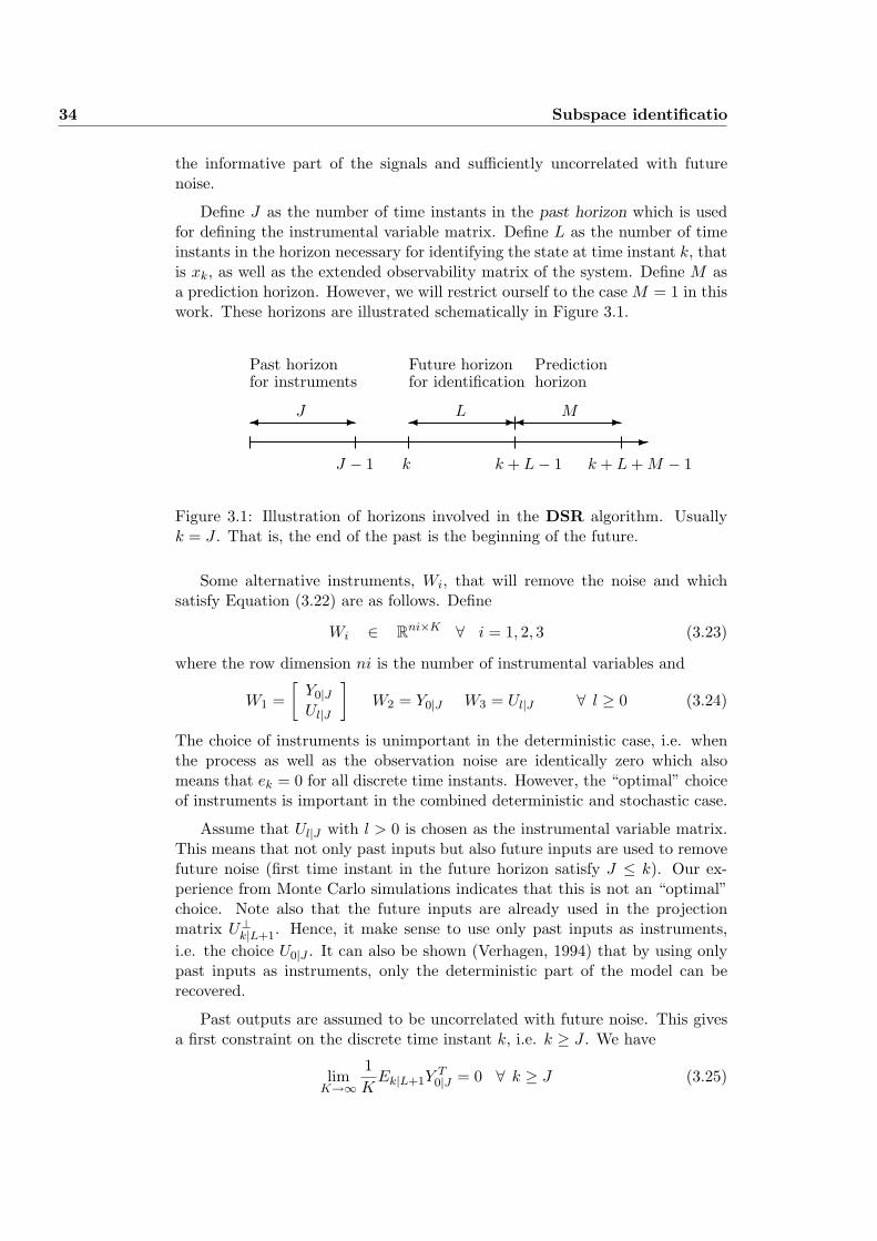
Define J as the number of time instants in the past horizon which is usedfor defining the instrumental variable matrix. Define L as the number of timeinstants in the horizon necessary for identifying the state at time instant k, thatis xk, as well as the extended observability matrix of the system. Define M asa prediction horizon. However, we will restrict ourself to the case M = 1 in thiswork. These horizons are illustrated schematically in Figure 3.1.
-¾ - ¾ -¾ -
Past horizon Future horizon
J L M
J − 1 k k + L− 1 k + L + M − 1
for identificationfor instrumentsPredictionhorizon
Figure 3.1: Illustration of horizons involved in the DSR algorithm. Usuallyk = J . That is, the end of the past is the beginning of the future.
Some alternative instruments, Wi, that will remove the noise and whichsatisfy Equation (3.22) are as follows. Define
Wi ∈ Rni×K ∀ i = 1, 2, 3 (3.23)
where the row dimension ni is the number of instrumental variables and
W1 =[
Y0|JUl|J
]W2 = Y0|J W3 = Ul|J ∀ l ≥ 0 (3.24)
The choice of instruments is unimportant in the deterministic case, i.e. whenthe process as well as the observation noise are identically zero which alsomeans that ek = 0 for all discrete time instants. However, the “optimal” choiceof instruments is important in the combined deterministic and stochastic case.
Assume that Ul|J with l > 0 is chosen as the instrumental variable matrix.This means that not only past inputs but also future inputs are used to removefuture noise (first time instant in the future horizon satisfy J ≤ k). Our ex-perience from Monte Carlo simulations indicates that this is not an “optimal”choice. Note also that the future inputs are already used in the projectionmatrix U⊥
k|L+1. Hence, it make sense to use only past inputs as instruments,i.e. the choice U0|J . It can also be shown (Verhagen, 1994) that by using onlypast inputs as instruments, only the deterministic part of the model can berecovered.
Past outputs are assumed to be uncorrelated with future noise. This givesa first constraint on the discrete time instant k, i.e. k ≥ J . We have
limK→∞
1K
Ek|L+1YT0|J = 0 ∀ k ≥ J (3.25)
3.4 System Identification and Realization 35
This statement can be proved from Equations (3.16) and (3.20). By incorpo-rating past outputs as instruments we are also able to recover the stochasticpart of the model. Note that the states which are exited from the known inputsare not necessarily the same as those which are exited from the unknown pro-cess noise variables. It is necessary that all states are exited from both knownand unknown inputs and that they are observable from the output, in order toidentify them.
Hence, the following past inputs and past outputs instrumental variablematrix is recommended to remove future noise from the model
W1 =[
Y0|JU0|J
]∈ RJ(m+r)×K ∀ J ≥ 1 (3.26)
A consistent equation for A is then given by the following autonomous matrixequation
Zk+1|L = AZk|L ∀ k ≥ J (3.27)
where
Zk+1|Ldef= 1
K Yk+1|LU⊥k|L+1W
Ti ∈ RmL×ni (3.28)
Zk|Ldef= 1
K Yk|LU⊥k|L+1W
Ti ∈ RmL×ni (3.29)
Equation (3.27) is consistent because Wi, given by Equations (3.23) and (3.24),satisfies Equation (3.22). See also Equation (3.25).
We can now prove that the column space of the matrix Zk|L coincides withthe column space of the extended observability matrix OL, when the identifica-tion (future) horizon parameter L is chosen great enough to observe all statesand the past horizon parameter J is chosen adequately. Using Equations (3.16)and (3.29) with the past inputs and past outputs instrumental variable matrixgives
Zk|L =1K
Yk|LU⊥k|L+1W
T1 = OLXkU
⊥k|L+1
1K
W T1 ∈ RmL×J(m+r) (3.30)
Assume that both the row and column dimensions of Zk|L are greater or equalto the number of states, i.e., Lm ≥ n and J(m + r) ≥ n, and that L is chosensuch that the system is observable. The dimension of the column space of theleft hand side matrix must be equal to the system order, i.e. rank(Xk) = n.Hence,
rank(Zk|L) = rank(1K
Yk|LU⊥k|L+1W
T1 ) = rank(OLXkU
⊥k|L+1
1K
W T1 ) = n (3.31)
The row constraints have a theoretical lower limit. From system theory weknow that a number of L ≥ n − rank(D) + 1 observations of the output issufficient in order to observe the states of a linear system, Kalman, Falb and
36 Subspace identificatio
Arbib (1969), p. 37. However, the theoretical lower limit is the ceiling functionL = dn/me, defined as the integer ratio n/m rounded towards plus infinity.
From the column dimension we must ensure that the past horizon J fordefining the instrumental variable matrix must satisfy J(m + r) ≥ n. Hence,the theoretical lower limit is J = dn/(m + r)e.
The maximum system order which can be specified by the user for a specifiedchoice of the parameter L is n = Lm. In this case the observability matrix canbe estimated as the column space of Zk|L only if the past horizon parameter Jis chosen such that J(m + r) ≥ Lm. A reasonable choice is therefore J = L.
Monte Carlo simulation experiments shows a relatively constant statisticalbehavior of the estimates as a function of the past horizon parameter J . Hence,we simply recommend putting J = L.
We have the following algorithm for analysis and modeling of system dy-namics.
Algorithm 3.4.1 (System order, n, and the pair (D,A))Given the positive integer parameters L and J and the matrices Zk+1|L andZk|L with k ≥ J which satisfy the autonomous matrix equation
Zk+1|L = AZk|L (3.32)
where
A = OLA(OTLOL)−1OT
L (3.33)
and OL is the extended observability matrix for the pair (A,D).1. The system order nDetermine the Singular Value Decomposition (SVD)
Zk|L = USV T (3.34)
where U ∈ RmL×mL, S ∈ RmL×ni and V ∈ Rni×ni are given by
U =[
U1 U2
]S =
[Sn 00 S2
]V =
[V1 V2
](3.35)
where Sn ∈ Rn×n and n is the number of “non-zero” singular values of Zk|L,which is equal to the system order. n is determined by inspection of the “non-zero” diagonal elements of S or SST . The term U2S2V
T2 represents the error
by estimating the system order as the n first principal singular values.2. The extended observability matrix OL for the pair (D,A)The (extended) observability matrix can be taken directly as the first left partin U , i.e. U1. We have
OL = U(1 : Lm, 1 : n) = U1 (3.36)
3. The system matrix AThe system matrix A can be determined as
A = OTLZk+1|LV
[S−1
n
0
]= UT
1 Zk+1|LV1S−1n (3.37)
3.4 System Identification and Realization 37
4. The system output matrix DThe matrix D can be taken as the m×n upper sub-matrix in the observabilitymatrix OL, i.e.
D = U(1 : m, 1 : n) (3.38)
5. The extended system matrix AWe have
A = OLA(OTLOL)−1OT
L = Zk+1|LV1S−1n UT
1 (3.39)
4
Note that it can be difficult to estimate the system order as the non-zero or largesingular values of the matrix Zk|L when the signal to noise ratio is “small”. Inpractice, the model order is chosen by a trial and error procedure combined withboth model validation and physical knowledge of the data generating process.A procedure for chosing the model order from some statistical test is possibile,see e.g. Ch. 9.6 in Aoki (1990).
We have chosen OL = U1 in Step 2 for simplicity, because we have OTLOL =
In×n in this case. This gives an output normal realization when L → ∞. The
algorithm can also be formulated with the choice OL = U1S12n which gives a bal-
anced realization when L →∞. OTLOL is equal to the observability grammian
as L tends to infinity because, in this case, DAL−1 tends to zero. A third choiceis OL = U1Sn which gives an input normal realization. These definitions areattributable to Moore (1981). These choices only represent different scalingsof the column space and give similar state space model matrices. The scalingdoes not affect the statistical properties of the algorithm.
3.4.2 Realization of the Deterministic Sub-system
At this stage the system matrices A and D as well as the extended observabilitymatrix OL are known, see Section 3.4.1. In order to obtain a complete realiza-tion for the deterministic part of the system we need to compute the systemmatrices B and E.
There are many alternatives for extracting the B and E matrices. See e.g.Section 3.5.2 for an alternative to the method presented below.
A consistent estimate of the B matrix can be computed from
B1K
Uk|L+1UTk|L+1 =
1K
(Yk+1|L − AYk|L)UTk|L+1 (3.40)
where A is determined from Algorithm 3.4.1, because
limK→∞
C1K
Ek|L+1UTk|L+1 = 0 ∀ k ≥ 0 (3.41)
38 Subspace identificatio
For known data and system matrices A and D, Equation (3.40) can be writtenas an over determined set of linear equations in the unknown system matricesB and E .
We will in the rest of this section discuss the simpler solution when Uk|L+1UTk|L+1
is non-singular. The matrix B can be computed directly from Equation (3.40)in this case. We refer to Section 3.5.2 for the case when Uk|L+1U
Tk|L+1 is singu-
lar. The system matrices B and E can be extracted from B. E is given directlyas the lower right m× r sub-matrix of B. We have
E = B(m(L− 1) + 1 : mL, rL + 1 : r(l + 1)) (3.42)
B is given as a function of the block columns in B and the matrices A and OL.A and OL are known from Algorithm 3.4.1. Define
Bi = B(1 : mL, r(i− 1) + 1 : ri) 1 ≤ i ≤ L + 1 (3.43)
as block column number i of B. We have
OLB =L+1∑
i=1
Ai−1Bi (3.44)
and
B =L+1∑
i=1
Ai−1(OTLOL)−1OT
LBi (3.45)
One strategy for recursively extracting the B, E, HdL and OLB matrices is as
follows.
Algorithm 3.4.2 Determination of HdL, OLB, E and B from known B, OL
and A.
A = OLA(OTLOL)−1OT
L
EL = BL+1
E = EL(m(L− 1) + 1 : mL, 1 : m)for i = 1, . . . , L
EL−i = BL−i+1 + AEL−i+1
if i < LEL−i(1 : r(L− i− 1), 1 : r) = zeros(r(L− i− 1), r)
endendOLB = E0
B = (OTLOL)−1OT
LOLB
4
The lower block triangular Toeplitz matrix HdL is given by the block columns
E1, · · ·, EL according to Equations (3.14) and (3.5).
3.4 System Identification and Realization 39
3.4.3 Realization of the Stochastic Sub-system
This section is mainly concerned with the problem of identifying the stochasticpart of the system. However, for natural reasons most of the results in Sections3.4.1 and 3.4.2 are extended and resolved in parallel.
The ESSM, Equation (3.7), gives a relation between the future data matricesand the SSM matrices. The following extension of the ESSM can be proved
Yk|L+1 = OL+1AkO†
JY0|J
+[
OL+1Cdk Hd
L+1
] [U0|kUk|L+1
]
−[
OL+1AkO†
JHdJ 0(L+1)m×(k+L+1−J)r
] [U0|JUJ |k+L+1−J
]
+[
OL+1Csk Hs
L+1
] [E0|kEk|L+1
]
−[
OL+1AkO†
JHsJ 0(L+1)m×(k+L+1−J)r
] [E0|JEJ |k+L+1−J
](3.46)
Assume k = J for the sake of simplicity. Then we have
YJ |L+1 = OL+1AJO†
JY0|J
+[
OL+1CdJ −OL+1A
JO†JHd
J HdL+1
] [U0|JUJ |L+1
]
+[
OL+1CsJ −OL+1A
JO†JHs
J HsL+1
] [E0|JEJ |L+1
](3.47)
This last equation nicely shows the connection between the past and futuredata matrices and the unknown model matrices. As we will see, it also yieldssome important results. We have the following projection
YJ |L+1
UJ |L+1
U0|JY0|J
⊥
=[
OL+1CsJ −OL+1A
JO†JHs
J HsL+1
]
E0|J
UJ |L+1
U0|JY0|J
⊥
EJ |L+1
UJ |L+1
U0|JY0|J
⊥
(3.48)
The projection of future inputs, past inputs and outputs onto the null-space offuture noise is equal to EJ |L+1. We have separated the deterministic part ofthe system from the data by the projection in Equation (3.48). Hence we havethe following theorem concerning the stochastic part of the system
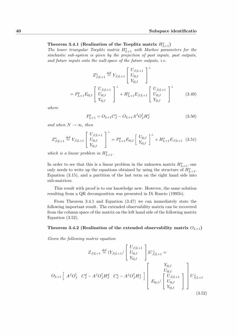
40 Subspace identificatio
Theorem 3.4.1 (Realization of the Toeplitz matrix HsL+1)
The lower triangular Toeplitz matrix HsL+1 with Markov parameters for the
stochastic sub-system is given by the projection of past inputs, past outputs,and future inputs onto the null-space of the future outputs, i.e.
ZsJ |L+1
def= YJ |L+1
UJ |L+1
U0|JY0|J
⊥
= P sL+1E0|J
UJ |L+1
U0|JY0|J
⊥
+ HsL+1EJ |L+1
UJ |L+1
U0|JY0|J
⊥
(3.49)
where
P sL+1 = OL+1C
sJ −OL+1A
JO†JHs
J (3.50)
and when N →∞, then
ZsJ |L+1
def= YJ |L+1
UJ |L+1
U0|JY0|J
⊥
= P sL+1E0|J
[U0|JY0|J
]⊥+ Hs
L+1EJ |L+1 (3.51)
which is a linear problem in HsL+1.
In order to see that this is a linear problem in the unknown matrix HsL+1, one
only needs to write up the equations obtained by using the structure of HsL+1,
Equation (3.15), and a partition of the last term on the right hand side intosub-matrices.
This result with proof is to our knowledge new. However, the same solutionresulting from a QR decomposition was presented in Di Ruscio (1995b).
From Theorem 3.4.1 and Equation (3.47) we can immediately state thefollowing important result. The extended observability matrix can be recoveredfrom the column space of the matrix on the left hand side of the following matrixEquation (3.52).
Theorem 3.4.2 (Realization of the extended observability matrix OL+1)
Given the following matrix equation
ZJ |L+1def= (YJ |L+1/
UJ |L+1
U0|JY0|J
)U⊥
J |L+1 =
OL+1
[AJO†
J CdJ −AJO†
JHdJ Cs
J −AJO†JHs
J
]
Y0|JU0|J
E0|J/
UJ |L+1
U0|JY0|J
U⊥J |L+1
(3.52)
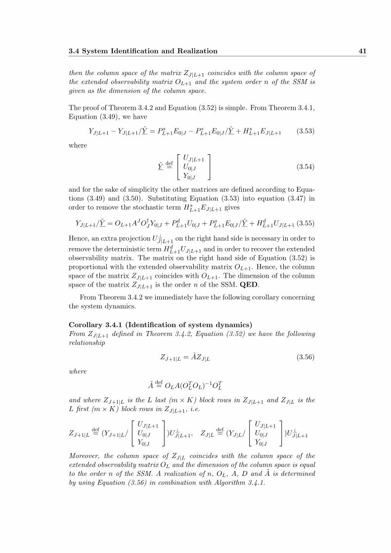
3.4 System Identification and Realization 41
then the column space of the matrix ZJ |L+1 coincides with the column space ofthe extended observability matrix OL+1 and the system order n of the SSM isgiven as the dimension of the column space.
The proof of Theorem 3.4.2 and Equation (3.52) is simple. From Theorem 3.4.1,Equation (3.49), we have
YJ |L+1 − YJ |L+1/Y = P sL+1E0|J − P s
L+1E0|J/Y + HsL+1EJ |L+1 (3.53)
where
Ydef=
UJ |L+1
U0|JY0|J
(3.54)
and for the sake of simplicity the other matrices are defined according to Equa-tions (3.49) and (3.50). Substituting Equation (3.53) into equation (3.47) inorder to remove the stochastic term Hs
L+1EJ |L+1 gives
YJ |L+1/Y = OL+1AJO†
JY0|J + P dL+1U0|J + P s
L+1E0|J/Y + HdL+1UJ |L+1 (3.55)
Hence, an extra projection U⊥J |L+1 on the right hand side is necessary in order to
remove the deterministic term HdL+1UJ |L+1 and in order to recover the extended
observability matrix. The matrix on the right hand side of Equation (3.52) isproportional with the extended observability matrix OL+1. Hence, the columnspace of the matrix ZJ |L+1 coincides with OL+1. The dimension of the columnspace of the matrix ZJ |L+1 is the order n of the SSM. QED.
From Theorem 3.4.2 we immediately have the following corollary concerningthe system dynamics.
Corollary 3.4.1 (Identification of system dynamics)From ZJ |L+1 defined in Theorem 3.4.2, Equation (3.52) we have the followingrelationship
ZJ+1|L = AZJ |L (3.56)
where
Adef= OLA(OT
LOL)−1OTL
and where ZJ+1|L is the L last (m ×K) block rows in ZJ |L+1 and ZJ |L is theL first (m×K) block rows in ZJ |L+1, i.e.
ZJ+1|Ldef= (YJ+1|L/
UJ |L+1
U0|JY0|J
)U⊥
J |L+1, ZJ |Ldef= (YJ |L/
UJ |L+1
U0|JY0|J
)U⊥
J |L+1
Moreover, the column space of ZJ |L coincides with the column space of theextended observability matrix OL and the dimension of the column space is equalto the order n of the SSM. A realization of n, OL, A, D and A is determinedby using Equation (3.56) in combination with Algorithm 3.4.1.

42 Subspace identificatio
The matrix on the left hand side of Equation (3.52) can be shown to beequivalent to
ZJ |L+1 = YJ |L+1Wc (3.57)
Wcdef= U⊥
J |L+1WT1 (W1U
⊥J |L+1W
T1 )−1W1U
⊥J |L+1
Comparing Equation (3.57) with Equation (3.30) shows that these matrices arerelated. We have shown that the column space of both equations coincides withthe column space of the extended observability matrix. The difference can beviewed as a different column weighting matrix Wc, on the right hand side ofEquation (3.57). Equation (3.30) can be viewed as a special case factorizationof equation (3.57) with k = J and Wc = U⊥
J |L+1WT1 /K. Later in Section 3.6,
we will show that this last Equation (3.57) is extremely important and usefulin order to partly compare other subspace identification methods.
From Theorem 3.4.1 we have the following result concerning the stochasticpart of the system.
Theorem 3.4.3 (Realization of ∆ and C)Assume that the number of system input and output observations, N → ∞.Define
ZsJ |L+1
def= YJ |L+1
UJ |L+1
U0|JY0|J
⊥
(3.58)
then we have
ZsJ+1|L = AZs
J |L + CEJ |L+1 (3.59)
and
ZsJ+1|L(Zs
J |L)⊥ = CEJ |L+1(ZsJ |L)⊥
where
Cdef=
[OLC Hs
L
]− A[
HsL 0Lm×m
]
The covariance matrix of the innovations ∆ is estimated directly from the col-umn space of the left hand side matrix Equation (3.58), e.g.
ZsJ+L|1(Z
sJ |L)⊥ = FEJ+L|1(Zs
J |L)⊥ = FEJ+L|1 (3.60)
and
∆ = FF T (3.61)
when
EJ+L|1ETJ+L|1 = Im×m
4
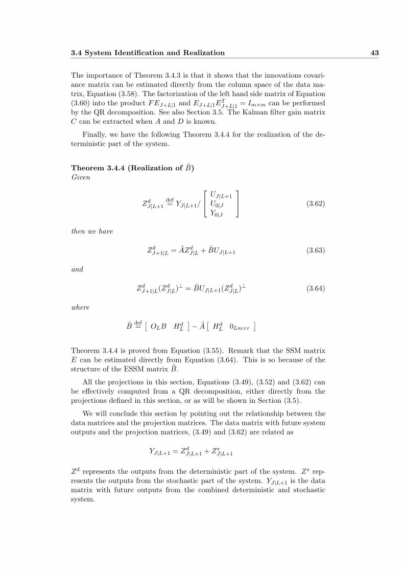
3.4 System Identification and Realization 43
The importance of Theorem 3.4.3 is that it shows that the innovations covari-ance matrix can be estimated directly from the column space of the data ma-trix, Equation (3.58). The factorization of the left hand side matrix of Equation(3.60) into the product FEJ+L|1 and EJ+L|1ET
J+L|1 = Im×m can be performedby the QR decomposition. See also Section 3.5. The Kalman filter gain matrixC can be extracted when A and D is known.
Finally, we have the following Theorem 3.4.4 for the realization of the de-terministic part of the system.
Theorem 3.4.4 (Realization of B)Given
ZdJ |L+1
def= YJ |L+1/
UJ |L+1
U0|JY0|J
(3.62)
then we have
ZdJ+1|L = AZd
J |L + BUJ |L+1 (3.63)
and
ZdJ+1|L(Zd
J |L)⊥ = BUJ |L+1(ZdJ |L)⊥ (3.64)
where
Bdef=
[OLB Hd
L
]− A[
HdL 0Lm×r
]
Theorem 3.4.4 is proved from Equation (3.55). Remark that the SSM matrixE can be estimated directly from Equation (3.64). This is so because of thestructure of the ESSM matrix B.
All the projections in this section, Equations (3.49), (3.52) and (3.62) canbe effectively computed from a QR decomposition, either directly from theprojections defined in this section, or as will be shown in Section (3.5).
We will conclude this section by pointing out the relationship between thedata matrices and the projection matrices. The data matrix with future systemoutputs and the projection matrices, (3.49) and (3.62) are related as
YJ |L+1 = ZdJ |L+1 + Zs
J |L+1
Zd represents the outputs from the deterministic part of the system. Zs rep-resents the outputs from the stochastic part of the system. YJ |L+1 is the datamatrix with future outputs from the combined deterministic and stochasticsystem.
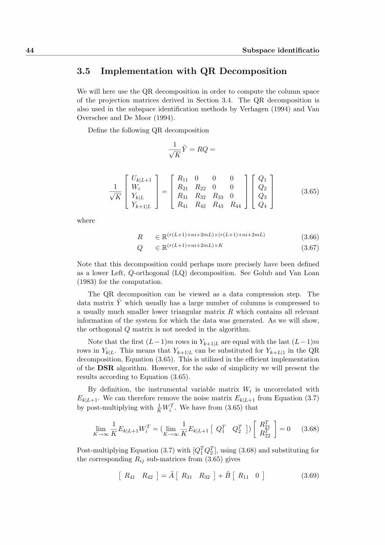
44 Subspace identificatio
3.5 Implementation with QR Decomposition
We will here use the QR decomposition in order to compute the column spaceof the projection matrices derived in Section 3.4. The QR decomposition isalso used in the subspace identification methods by Verhagen (1994) and VanOverschee and De Moor (1994).
Define the following QR decomposition
1√K
Y = RQ =
1√K
Uk|L+1
Wi
Yk|LYk+1|L
=
R11 0 0 0R21 R22 0 0R31 R32 R33 0R41 R42 R43 R44
Q1
Q2
Q3
Q4
(3.65)
where
R ∈ R(r(L+1)+ni+2mL)×(r(L+1)+ni+2mL) (3.66)Q ∈ R(r(L+1)+ni+2mL)×K (3.67)
Note that this decomposition could perhaps more precisely have been definedas a lower Left, Q-orthogonal (LQ) decomposition. See Golub and Van Loan(1983) for the computation.
The QR decomposition can be viewed as a data compression step. Thedata matrix Y which usually has a large number of columns is compressed toa usually much smaller lower triangular matrix R which contains all relevantinformation of the system for which the data was generated. As we will show,the orthogonal Q matrix is not needed in the algorithm.
Note that the first (L−1)m rows in Yk+1|L are equal with the last (L−1)mrows in Yk|L. This means that Yk+1|L can be substituted for Yk+L|1 in the QRdecomposition, Equation (3.65). This is utilized in the efficient implementationof the DSR algorithm. However, for the sake of simplicity we will present theresults according to Equation (3.65).
By definition, the instrumental variable matrix Wi is uncorrelated withEk|L+1. We can therefore remove the noise matrix Ek|L+1 from Equation (3.7)by post-multiplying with 1
K W Ti . We have from (3.65) that
limK→∞
1K
Ek|L+1WTi = ( lim
K→∞1K
Ek|L+1
[QT
1 QT2
])[
RT21
RT22
]= 0 (3.68)
Post-multiplying Equation (3.7) with [QT1 QT
2 ], using (3.68) and substituting forthe corresponding Rij sub-matrices from (3.65) gives
[R41 R42
]= A
[R31 R32
]+ B
[R11 0
](3.69)
3.5 Implementation with QR Decomposition 45
which gives one matrix equation for A and one for both A and B. We will in thenext Sections 3.5.1 and 3.5.2 show how the order n and the system quadruple(A,B,D, E) are computed from (3.69).
The stochastic part of the system, defined by the matrices C and ∆, iscomputed from
R43 − AR33 = CEk|L+1QT3 (3.70)
R44 = CEk|L+1QT4 (3.71)
This will be shown in Section 3.5.3.
Note that the QR decomposition compresses the possible large data matri-ces into a number of (smaller) matrices which contain the information of thesystem. It is also interesting that the matrices (information) which define thedeterministic part (A,B,D, E) and the stochastic part (∆, C) are separated bythe QR decomposition. The user must specify the parameter k ≥ J in Equation3.65. See Figure 3.1 for a definition of the horizons involved. We recommendputting k = J . The matrix W1 with l = 0, Equation (3.24), is recommendedfor Wi in 3.65.
3.5.1 Realization of A and D
We have from Equation (3.69) that
R42 = AR32 (3.72)
and we choose
Zk+1|L = R42 (3.73)
Zk|L = R32 = USV T (3.74)
in Algorithm (3.4.1) in order to determine A, D and the extended observabilitymatrix OL. The system order is determined by inspection of the dominantsingular values of S or SST .
Note that the first (L−1)m rows in R42 are equal to the last (L−1)m rowsin R32. This is utilized in the efficient implementation of the DSR algorithm,in order to reduce the computational work.
Note also that if A is computed as the projection of R32 onto R42 then Atakes a special canonical form. This is due to the common rows.
The A matrix may also be determined as follows. From the extended ob-servability matrix we have
O1def= OL(1 : (L− 1)m, 1 : n) (3.75)
O2def= OL(m + 1 : Lm, 1 : n) (3.76)
then
A = (OT1 O1)−1OT
1 O2 (3.77)
46 Subspace identificatio
However, we must put L =: L + 1 in this case if the extended observabilitymatrix is estimated as the left singular vectors in (3.74). This will increase thecomputational work. This last method is the so called shift invariance methodfor computing the transition matrix A from the extended observability matrix,Kung (1978). The shift invariance method is used in the subspace algorithms(N4SID) by Van Overschee and De Moor (1994) and (MOESP) by Verhagen(1994). The parameter which defines the number of block rows in the N4SIDand MOESP algorithms is denoted I. This parameter is related to the DSRparameter L as I = L + 1. This is one of the differences between the DSRalgorithm and the N4SID and MOESP algorithms.
This means that N4SID and MOESP computes a number Im = (L+1)mof singular values. However, the system order can only be chosen accordingto Lm of these singular values, i.e. the maximum system order which canbe chosen for a specified parameter I = L + 1 is n = Lm. For comparison,the DSR algorithm computes only a number Lm of singular values and themaximum system order which can be chosen for a specified parameter L isn = Lm. Hence, the DSR algorithm seems to be more consistent with respectto choosing the system order as the number of non-zero singular values.
The shift invariance method can be included in the DSR algorithm, butat a higher computational expense. This strategy can be described as follows.The extended observability matrix can be estimated from the column space ofthe matrix formed from R32 and R42. Compute the SVD
[R32
R42
]=
[U11 U12
U21 U22
] [Sn 00 0
] [V T
1
V T2
]=
[U11SnV T
1
U21SnV T1
]
We then have that A and D are determined from the shift invariance method,e.g. from the left singular vectors as follows
OL = U11 (3.78)OLA = U21 (3.79)
A = (UT11U11)−1UT
11U21 (3.80)D = U11(1 : m, 1 : n) (3.81)
3.5.2 Realization of B and E
We have from Equation (3.69) that
BR11 = R41 − AR31 (3.82)
B can be determined directly from (3.82) if the input u is persistently exitingof order L + 1. R11 is non singular in this case. We have
B = (R41 − AR31)RT11(R11R
T11)
−1 (3.83)
The B and E matrices are then extracted from B as pointed out in Section3.4.2.
3.5 Implementation with QR Decomposition 47
At this stage, the system order is identified (Algorithm 3.4.1). It is possibleto determine B and E if the input is only persistently exiting of order p + 1where Lmin ≤ p ≤ L, directly without recomputing the algorithm with L =Lmin or L = p. The minimal observability index, for a given system order, isLmin = n− rank(D) + 1 when n ≥ rank(D) and Lmin = 1 when n ≤ rank(D).
Define
Op = OL(1 : mp, 1 : n) (3.84)Ap = OpA(OT
p Op)−1OTp (3.85)
Rp11 = R11(1 : r(p + 1), 1 : r(p + 1)) (3.86)
Rp31 = R31(1 : mp, 1 : r(p + 1)) (3.87)
Rp41 = R41(1 : mp, 1 : r(p + 1)) (3.88)
We then have
BpRp11 = Rp
41 − ApRp31 (3.89)
This result is a consequence of Equation (3.7) with L substituted with p. Notethat the minimal observability index, for a given system order, is p = n −rank(D) + 1 when n ≥ rank(D). The B and E matrices are then extractedfrom Bp as shown in Section 3.4.2 and Algorithm 3.4.2 with L substituted withp.
3.5.3 Realization of C and ∆
Corollary 3.5.1 (Realization of C and ∆)Consider the lower left triangular matrix R, determined by the QR decompo-sition in Equation (3.65). An estimate of the square root of the innovationscovariance matrix is given by the m×m lower right sub-matrix of R, i.e.
F = R44(m(L− 1) + 1 : mL, m(L− 1) + 1 : mL) (3.90)
and the estimate of the innovations covariance matrix is
∆ = FF T (3.91)
Furthermore, when J > 1, then an estimate of the Kalman filter gain matrix Ccan be computed from
OLCF = R43(1 : mL, 1 : m) (3.92)
If F is non-singular, then we have
C = (OTLOL)−1OT
LR43(1 : mL, 1 : m)F−1 (3.93)
An estimate of the lower left block triangular Toeplitz matrix HsL for the stochas-
tic subsystem (D, A, CF, F ) is given by
HsL = R43(1 : mL,m + 1 : m(L + 1)) (3.94)
48 Subspace identificatio
The estimate of the lower left block triangular Toeplitz matrix for the stochasticsubsystem (D,A, C, I), according to Equation (3.15), can be formed from theblock columns F1, · · · , FL which can be computed from
[F1F F2F · · · FLF
]= R43(1 : mL,m + 1 : m(L + 1)) (3.95)
4
The stochastic subsystem is identified separately from the deterministic sub-system. The necessary separation into deterministic and stochastic subsystemsare implicitly done by the QR decomposition.
The first (L − 1)m rows in Yk+1|L are equal to the (L − 1)m last rows inYk|L. Q4 is uncorrelated with Uk|L+1, Wi, Yk|L and with the (L−1)m first rowsin Yk+1|L. The first (L − 1)m rows in Yk+1|LQT
4 and Ek|L+1QT4 are therefore
zero. We then have from (3.65) and the structure of C, given by (3.13) and(3.15), that
Yk+1|LQT4 = CEk|L+1Q
T4 = R44 =
0 0 · · · 00 0 0...
. . ....
0 0 · · · F
(3.96)
where R44 ∈ RLm×Lm. Hence, the square root of the innovations noise processcovariance matrix is estimated directly as the m×m lower left matrix, denotedF , in the lower triangular matrix R from the QR decomposition, Equation(3.65). Note that F also is lower left triangular and can be compared to aCholesky factorization of ∆. This result is believed to be of some importance.The result (3.91) is then clarified.
The matrices Qi, i = 1, 2, 3, 4, are orthogonal matrices and we have
1K
Ek|L+1QT3 =
F 0 · · · 00 F 0...
. . ....
0 0 · · · F0 0 · · · 0
∈ R(L+1)m×Lm (3.97)
Another strategy is then to compute OCF from Equations (3.70) and (3.97),and an algorithm similar to Algorithm 3.4.2. This is formulated in the followingCorollary 3.5.2.
Corollary 3.5.2 (Realization of C)Given the sub-matrices R43 and R33 from the QR decomposition in Equation(3.67) and the ESSM transition matrix A. Define according to Equation (3.70)
CFdef= R43 − AR33 (3.98)
The matrix OLCF can then be computed from CF , e.g. by a procedure similarto Algorithm 3.4.2.4
3.5 Implementation with QR Decomposition 49
This strategy is found from Monte Carlo simulations to be the best onewhen the past horizon parameter is J = 1, but no significant difference is foundwhen J > 1.
3.5.4 Special Remarks
One advantage of the QR implementation of the algorithm is that potential ill-conditioning of the covariance matrices are concentrated in a certain triangularmatrix. This ill-conditioning usually results from ill-conditioned noise processes(process noise and measurements noise) and from rounding-off errors. Note thatthe triangular matrix R is the square root of the covariance matrix (H = 1
K Y Y T
where Y is defined in (3.65)) and that the triangular matrix is computed withoutever computing the covariance matrix. The method can therefore be defined asnumerically stable.
The QR decomposition is not unique. The R matrix is post-multipliedby a diagonal permutation matrix E such that R := RE has positive diagonalelements. The diagonal elements of E are equal to the sign of the correspondingdiagonal elements of R which was the result from the QR decomposition. Notealso that Q := EQ and EE = I. This gives a more unique coordinate systemfor the estimated (A,B, D, E) quadruple. This scaling is also one of the reasonsfor the simple solutions for the C and ∆ matrices in Section 3.5.3. The scalingensures that the diagonal blocks of (3.97) gets the same sign.
Note that common rows in the data matrices Yk|L and Yk+1|L can be removedprior to obtaining the QR decomposition in equation (3.67). It is also clearfrom the above that the orthogonal Q matrix (QQT = I) is not needed in thealgorithm. This will reduce the computational effort considerably. In fact, theQR factorization works on a data matrix of size only r(2L+1)+m(2L+1)×Kand not of size r(2L + 1) + 3mL×K as indicated in (3.65).
Another strategy for determining R is to first compute H = 1K Y Y T where
Y is defined in (3.65) and then the SVD, H = USV T , followed by a QR de-composition of US
12 in order to obtain the lower triangular matrix, R. This
strategy reduced the number of flops and increased the accuracy of the R ma-trix when MATLAB was used for the computations. However, no significantdifference in the estimated models was observed. This strategy can be numeri-cally ill-conditioned due to possible rounding errors when forming the productof rows in Y with columns in Y T in order to compute the correlation matrixY Y T . This strategy is therefore not recommended.
Equation (3.82) is defined by the triangular factors for Equation (3.40) withk ≥ J .
BUk|L+1UTk|L+1 = Yk+1|LUT
k|L+1 − AYk|LUk|L+1 (3.99)
It is also possible to extract the triangular factors for
BU0|L+1UT0|L+1 = Y1|LUT
0|L+1 − AY0|LU0|L+1 (3.100)
50 Subspace identificatio
directly from the QR decomposition (3.65) when k = J = L. The first blockrow in UL|L+1 is equal to the last block row in U0|L+1. Hence, the matrices inEquation (3.100) can be defined from the lower triangular R matrix, equation(3.65). It is therefore natural to choose
B[
R11 R011
]=
[R41 R0
41
]− A[
R31 R031
](3.101)
for defining B and an equation for computing the B and E system matrices.Equation (3.101) consists of the triangular factors for both 1
K Uk|L+1UTk|L+1 and
1K U0|L+1U
T0|L+1. Equation (3.101) has effect for systems where the input signal
is poor with frequencies, but gives no additional effect compared to (3.82) fore.g. white noise inputs.
Note that the stochastic part of the model is determined from QR andSV Decompositions only. The Markov parameters and the square root of theinnovations covariance matrix are determined from a QR decomposition only.The Kalman filter gain matrix is determined from the Markov parameters andthe extended observability matrix. No matrix Lyapunov or non-linear matrixRiccati equations have to be solved.
The method has in this work been illustrated for systems which are notstrictly proper (only proper), i.e. the case when E 6= 0 in the underlying model(3.2). The method can also be implemented to handle proper systems, i.e.systems where E is known to be zero. This can be done by deleting the lastblock row in Uk|L+1 and the last block column in B, see Equation (3.7).
3.6 Comparison with Existing Algorithms
A comparison with the DSR algorithm and three different subspace algorithmswill be given, namely N4SID, Van Overschee and De Moor (1994), CVA,Larimore (1983), (1990) and PO-MOESP, Verhagen (1994).
The first and common step in subspace identification algorithms is to es-timate the extended observability matrix from the column space of a knowndata matrix. We will therefore concentrate our discussion on the similaritiesand differences in which these methods estimate the extended observability ma-trix. We will only briefly discuss how the system matrices are estimated by thedifferent methods.
It is shown in Van Overschee and De Moor (1995) that the different methodsare related through certain row and column weightings with the N4SID datamatrix as the key matrix.
We will below present a different approach, with the matrix ZJ |L+1 definedin Section 3.4.3, Theorem 3.4.2 and Equation (3.57), as the key matrix.
Multiplying Equation (3.57) from left with an extra row weighting matrixWr and using the SVD as discussed in Algorithm 3.4.1 gives
WrZJ |L+g = WrYJ |L+gWc = U1SnV T1 + U2S2V
T2 (3.102)
3.6 Comparison with Existing Algorithms 51
where g is an integer parameter and
Wcdef= U⊥
J |L+1WT1 (W1U
⊥J |L+1W
T1 )−1W1U
⊥J |L+1
The extended observability matrix can be estimated as, e.g.
OL+g = W−1r U1 (3.103)
where Wr is a non-singular matrix. The matrix Wc is symmetric and can bewritten as
Wcdef= U⊥
J |L+1WT1 (W1U
⊥J |L+1W
T1 )−
12
︸ ︷︷ ︸W 2
c
(W1U⊥J |L+1W
T1 )−
12 W1U
⊥J |L+1︸ ︷︷ ︸
(W 2c )T
(3.104)
From the above factorization of the matrix Wc we have at least four matrices(W i
c , i = 1, · · · , 4) which all have essentially the same column space as Wc, i.e.
W 1c = U⊥
J |L+1WT1 (W1U
⊥J |L+1W
T1 )−1W1U
⊥J |L+1
W 2c = U⊥
J |L+1WT1 (W1U
⊥J |L+1W
T1 )−
12
W 3c = U⊥
J |L+1WT1 (W1U
⊥J |L+1W
T1 )−1K
W 4c = U⊥
J |L+1WT1
1K
W 5c = U⊥
J |L+1
The matrix W 5c is sufficient only for purely deterministic systems and is shown
for the sake of completeness.
These column weighting matrices are used in the DSR algorithm whichis presented in this work. The past horizon parameter J is usually chosen asJ ≥ L. The parameter g = 0 in Equation (3.102) and the row weighting matrixis the Lm×Lm identity matrix, denoted Wr = ILm. Algorithm 3.4.1 is used inorder to identify the extended observability matrix OL from the column spaceof the matrix ZJ |L.
We will now illustrate the DSR algorithm’s similarity and difference to twopublished algorithms, CVA by Larimore (1990) and PO-MOESP by Verhagen(1994).
3.6.1 PO-MOESP
The PO-MOESP algorithm in Verhagen (1994) estimates the extended ob-servability matrix OL+1 from Equations (3.102) and (3.103) with the followingmatrices
Wc = U⊥L+1|L+1W
T1 (W1U
⊥L+1|L+1W
T1 )−1W1U
⊥L+1|L+1
Wr = I(L+1)m
g = 1
PO-MOESP(3.105)
From Theorem 3.4.2 and the factorization in Equation (3.104) we conclude thatthe two algorithms PO-MOESP and DSR estimate the extended observability
52 Subspace identificatio
matrix from a known data matrix which essentially has the same column space.The only difference is that PO-MOESP estimates the extended observabilitymatrix OL+1 (of larger size than DSR does) in order to use the shift invariancemethod for extracting the system matrix A as explained in Section 3.5.1.
Using the triangular factors from the QR decomposition in Section 3.5, wehave
R32RT22(R22R
T22)
−1R22Q2 = (U1SnV T1 + U2S2V
T2 )Q2 (3.106)
where the orthogonal matrix Q2 is not needed because the column space canbe estimated as the matrix U1.
A major difference is that the PO-MOESP algorithm does not estimate thestochastic part of the model. DSR estimates the Kalman gain and innovationscovariance matrix directly from the data as shown in Sections 3.4.3 and 3.5.3.
3.6.2 Canonical Variate Analysis (CVA)
The CVA algorithm in Larimore (1990) estimates the extended observabilitymatrix OL+1 from Equations (3.102) and (3.103) with the following matrices
Wc = U⊥L+1|L+1W
T1 (W1U
⊥L+1|L+1W
T1 )−
12
Wr = (YL+1|L+1U⊥L+1|L+1Y
TL+1|L+1)
− 12
g = 1
CVA (3.107)
As we can see, the column weighting matrix Wc used by the CVA algorithmfits into the factorization in Equation (3.104). A difference is that the CVAalgorithm uses a row weighting matrix Wr.
The only difference is that the DSR algorithm takes the SVD of a matrixof size only Lm× J(r + m) where usually J = L, in order to identify OL. Theother methods take the SVD of a matrix of size (L + 1)m× J(r + m), in orderto identify OL+1. This is to separate out the sub-matrices OL and OLA fromOL+1. See also Section 3.5.1 for a discussion.
From Theorem 3.4.2 and the factorization in Equation (3.104) we concludethat the two algorithms CVA and DSR essentially have the same columnspace.
An interpretation of the CVA algorithm is that the system order is esti-mated as the number of principal angles between the matrix YL+1|L+1U
⊥L+1|L+1
and W1U⊥L+1|L+1 different from π/2. The principal angles can be effectively
computed using the SVD, see e.g. Van Overschee (1995), p. 29 and Golub andVan Loan (1989), p. 428.
By using the triangular factors as shown in Section 3.5 we get the followingmethod for computing the principal angles
(R32RT32 + R33R
T33)
− 12 R32R
T22(R22R
T22)
− 12 = U1SnV T
1 + U2S2VT2 (3.108)
3.6 Comparison with Existing Algorithms 53
The system order is here identified as the number of singular values equal toone.
The next step in the CVA algorithm is to define a memory which definesa valid sequence of system states. The system matrices can then be estimatedfrom a least squares problem.
3.6.3 N4SID
The N4SID algorithm is different. The following weighting matrices are used
Wc = U⊥L+1|L+1W
T1 (W1U
⊥L+1|L+1W
T1 )−1W1
Wr = I(L+1)m
g = 1
N4SID (3.109)
The column weighting matrix used in the N4SID algorithm does not generallyhave the same column space as Wc or any of the column weighting matriceswhich result from Equation (3.104) and Theorem 3.4.2. This is possibly thereason for why N4SID gives bad results for deterministic input signals.
In Viberg (1995) it is pointed out that only the difference between the PO-MOESP and N4SID algorithms is the extra projection U⊥
L+1|L+1. However, itis also claimed that the resulting subspace estimates should therefore have verysimilar properties. From Theorem 3.4.2 and the above discussion we concludethat this conclusion in Viberg (1995) is wrong. This is illustrated in example2, Section 3.7.2.
From the above discussion we have the following relationship between thecolumn weighting matrix Wc in Equation (3.104) and the matrix Wc in (3.109)used by N4SID.
Wc = WN4sidc U⊥
L+1|L+1 (3.110)
In Theorem 3.4.2, Equations (3.52) and (3.55), it is proved that the extraprojection U⊥
L+1|L+1 is necessary in order to remove the deterministic termHd
L+1UL+1|L+1 and establish the data matrix ZL+1|L+1 which has the samecolumn space as the extended observability matrix. See also Example 2, Section3.7.2, for an illustration.
The N4SID method computes the SVD of the data matrix defined in Equa-tion (3.102) with the above matrices Wr and Wc, Equation (3.109). If thetriangular factors as shown in Section 3.5 are used then we have
R32RT22(R22R
T22)
−1[R21R22][
Q1
Q2
]= (U1SnV T
1 + U2S2VT2 )
[Q1
Q2
](3.111)
The orthogonal matrices Q1 and Q2 are not used. The system order is identifiedas the number of non-zero singular values and the extended observability matrixOL+1 is estimated from the column space. The rest of the N4SID algorithmcan briefly be described as follows. From the extended observability matrix
54 Subspace identificatio
OL+1 and the system data, a valid sequence of system states are estimatedand a least squares problem is solved in order to construct the system matricesA,B, D, E. The covariance matrices for the process and measurements noiseare then identified from a residual, and a Riccati equation is solved in orderto construct the Kalman filter gain matrix C and the innovations covariancematrix ∆.
The DSR method does not use state sequences and the Kalman gain matrixC and the innovations covariance matrix ∆ are constructed directly from thedata, without recursions of non-linear matrix Riccati equations.
3.6.4 Main Differences and Similarities
Both of the algorithms N4SID and CVA estimate in the first instance a se-quence of states. When the states are known, the state space model matricescan be determined by simple linear regression. Both methods must solve amatrix Riccati equation in order to identify the Kalman filter gain and theinnovations covariance matrices.
The DSR algorithm is based on first writing up an extended state spacemodel (ESSM) where the unknown states are eliminated from the problem.The ESSM shows us the relationship between the known data matrices and theSSM matrices. Hence, the DSR algorithm does not have any problems withunknown states; unknown initial values etc. The state space model matrices arethen extracted from the ESSM. DSR estimates the Kalman gain and innova-tions covariance matrices (stochastic part of the model) directly from the data,without recursions of non-linear matrix equations, e.g. the Riccati equation.
The PO-MOESP algorithm does not estimate the stochastic part of themodel.
We have shown that the CVA, PO-MOESP and DSR algorithms givesconsistent estimates of the extended observability matrix. The algorithms fitinto the same Theorem 3.4.2. We have shown that the N4SID algorithm ingeneral does not give consistent estimates of the extended observability matrix.However, it will give consistent results if an extra projection of future inputs isincluded. From the above discussion we have the following relationship betweenthe column weighting matrix Wc in Equation (3.104) and the matrices used byPO-MOESP, CVA and N4SID. See (3.105), (3.107) and (3.109).
Wc = WPO-MOESPc = WCVA
c (WCVAc )T = WN4sid
c U⊥L+1|L+1
These are the most important similarities and differences between the methodpresented in this work and previously published methods.
3.7 Numerical Examples 55
3.7 Numerical Examples
3.7.1 Example 1: Monte Carlo Simulation
A single input single output (SISO) system with one state is chosen to com-pare the algorithm presented in this paper, entitled DSR (Deterministic andStochastic System Identification and Realization), with two other algorithms,CVA (which stands for Canonical Variate Analysis, Larimore (1983), (1990))and the prediction error method implemented in the MATLAB function AR-MAX (i.e., in the system identification toolbox, Ljung (1991)).
xk+1 = 0.9xk + 0.5uk + 0.6ek (3.112)yk = 1.0xk − 1.0uk + ek (3.113)
Three types of input signals were used. One input equal to a sum of four sinusoidsignals, u1, one input equal to a white noise signal with unit covariance, u2,and one equal to a sine, u3.
u1 uk = 0.2(sin(k
25) + sin(
k
10) + sin(
k
5) + sin(k))
u2 White noise, unit covarianceu3 uk = sin(k)
For each input the time series (yk, uk) was generated by simulating the modelwith 100 different white noise sequences ek, also with unit variance.
The DSR algorithm parameter L was changed from 1 to 5 and the CVAparameter I from 2 to 6. For each L and I, the mean and standard deviation ofthe parameters of the 100 different estimated models are presented in Tables 3.1to 3.6. The results obtained by the ARMAX algorithm are also shown in thetables. See Ljung (1991) for the description of the parameters nn = [1, 2, 1, 0]which is used as arguments for ARMAX.
The true deterministic system quadruple is denoted (a, b, d, e) := (0.9, 0.5,1,−1) and the deterministic steady state gain and deterministic zero are de-noted Hd(1) = 4.0 and pd(1) = 1.4, respectively. The parameters in the stochas-tic part of the model are (c, ∆) := (0.6, 1). The stochastic steady state gainand stochastic zero are denoted Hs(1) = 7.0 and ps(1) = 0.3, respectively. Thesignal to noise ratio is approximately 0.4, hence, the identification problem isnot simple.
The CVA algorithm sometimes estimated systems with negative (b,d) pa-rameters, i.e. sometimes an estimated quadruple (a,b,d,e) and sometimes (a,-b,-d,e). This happened with the algorithm parameter I = 3 and with a randominput signal. It is believed that this can be avoided by using a scaling similarto that presented in Section 3.5.4.
The results are very good for both the DSR and the CVA algorithms, seeTables 3.1 and 3.2. There are small differences in the estimated models forboth methods when N is large, see Tables 3.1 and 3.2. This indicates that the
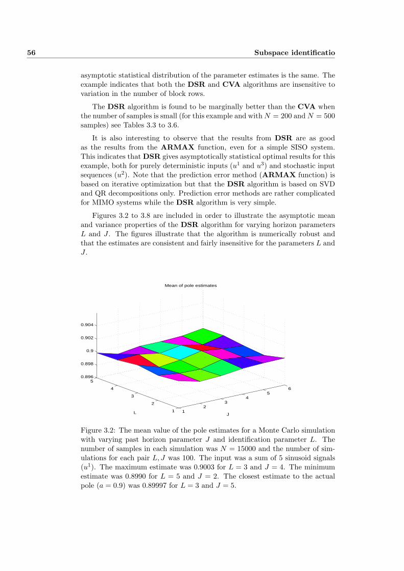
56 Subspace identificatio
asymptotic statistical distribution of the parameter estimates is the same. Theexample indicates that both the DSR and CVA algorithms are insensitive tovariation in the number of block rows.
The DSR algorithm is found to be marginally better than the CVA whenthe number of samples is small (for this example and with N = 200 and N = 500samples) see Tables 3.3 to 3.6.
It is also interesting to observe that the results from DSR are as goodas the results from the ARMAX function, even for a simple SISO system.This indicates that DSR gives asymptotically statistical optimal results for thisexample, both for purely deterministic inputs (u1 and u3) and stochastic inputsequences (u2). Note that the prediction error method (ARMAX function) isbased on iterative optimization but that the DSR algorithm is based on SVDand QR decompositions only. Prediction error methods are rather complicatedfor MIMO systems while the DSR algorithm is very simple.
Figures 3.2 to 3.8 are included in order to illustrate the asymptotic meanand variance properties of the DSR algorithm for varying horizon parametersL and J . The figures illustrate that the algorithm is numerically robust andthat the estimates are consistent and fairly insensitive for the parameters L andJ .
12
34
56
1
2
3
4
50.896
0.898
0.9
0.902
0.904
L J
Mean of pole estimates
Figure 3.2: The mean value of the pole estimates for a Monte Carlo simulationwith varying past horizon parameter J and identification parameter L. Thenumber of samples in each simulation was N = 15000 and the number of sim-ulations for each pair L, J was 100. The input was a sum of 5 sinusoid signals(u1). The maximum estimate was 0.9003 for L = 3 and J = 4. The minimumestimate was 0.8990 for L = 5 and J = 2. The closest estimate to the actualpole (a = 0.9) was 0.89997 for L = 3 and J = 5.
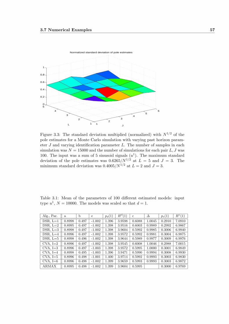
3.7 Numerical Examples 57
12
34
56
1
2
3
4
50
0.2
0.4
0.6
0.8
1
L J
Normalized standard deviation of pole estimates
Figure 3.3: The standard deviation multiplied (normalized) with N1/2 of thepole estimates for a Monte Carlo simulation with varying past horizon param-eter J and varying identification parameter L. The number of samples in eachsimulation was N = 15000 and the number of simulations for each pair L, J was100. The input was a sum of 5 sinusoid signals (u1). The maximum standarddeviation of the pole estimates was 0.6265/N1/2 at L = 5 and J = 3. Theminimum standard deviation was 0.4005/N1/2 at L = 2 and J = 3.
Table 3.1: Mean of the parameters of 100 different estimated models: inputtype u1, N = 10000. The models was scaled so that d = 1.
Alg., Par. a b e pd(1) Hd(1) c ∆ ps(1) Hs(1)
DSR, L=1 0.8998 0.497 -1.002 1.396 3.9598 0.6088 1.0045 0.2910 7.0910
DSR, L=2 0.8995 0.497 -1.002 1.398 3.9516 0.6003 0.9989 0.2992 6.9867
DSR, L=3 0.8998 0.497 -1.002 1.398 3.9604 0.5992 0.9985 0.3006 6.9940
DSR, L=4 0.8996 0.497 -1.002 1.398 3.9572 0.5992 0.9981 0.3004 6.9875
DSR, L=5 0.8998 0.496 -1.002 1.398 3.9644 0.5989 0.9977 0.3009 6.9976
CVA, I=2 0.8996 0.497 -1.002 1.398 3.9545 0.6008 1.0046 0.2988 7.0015
CVA, I=3 0.8996 0.497 -1.003 1.398 3.9572 0.5995 1.0000 0.3001 6.9849
CVA, I=4 0.8998 0.495 -1.003 1.396 3.9471 0.5990 0.9994 0.3008 6.9930
CVA, I=5 0.8996 0.498 -1.001 1.400 3.9714 0.5992 0.9993 0.3003 6.9830
CVA, I=6 0.8996 0.498 -1.002 1.399 3.9659 0.5993 0.9993 0.3003 6.9872
ARMAX 0.8995 0.498 -1.002 1.399 3.9604 0.5995 0.3000 6.9769
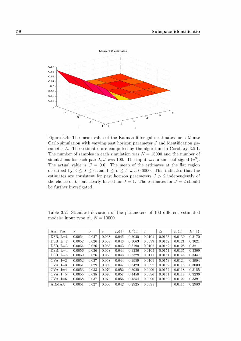
58 Subspace identificatio
12
34
56
1
2
3
4
5
0.57
0.58
0.59
0.6
0.61
0.62
0.63
0.64
L J
Mean of C estimates
Figure 3.4: The mean value of the Kalman filter gain estimates for a MonteCarlo simulation with varying past horizon parameter J and identification pa-rameter L. The estimates are computed by the algorithm in Corollary 3.5.1.The number of samples in each simulation was N = 15000 and the number ofsimulations for each pair L, J was 100. The input was a sinusoid signal (u3).The actual value is C = 0.6. The mean of the estimates at the flat regiondescribed by 3 ≤ J ≤ 6 and 1 ≤ L ≤ 5 was 0.6000. This indicates that theestimates are consistent for past horizon parameters J > 2 independently ofthe choice of L, but clearly biased for J = 1. The estimates for J = 2 shouldbe further investigated.
Table 3.2: Standard deviation of the parameters of 100 different estimatedmodels: input type u1, N = 10000.
Alg., Par. a b e pd(1) Hd(1) c ∆ ps(1) Hs(1)
DSR, L=1 0.0054 0.027 0.068 0.045 0.3020 0.0101 0.0153 0.0130 0.3170
DSR, L=2 0.0052 0.026 0.068 0.043 0.3063 0.0099 0.0152 0.0121 0.3021
DSR, L=3 0.0054 0.026 0.068 0.043 0.3190 0.0102 0.0152 0.0128 0.3211
DSR, L=4 0.0056 0.026 0.068 0.044 0.3236 0.0105 0.0151 0.0135 0.3309
DSR, L=5 0.0059 0.026 0.068 0.043 0.3328 0.0111 0.0151 0.0145 0.3447
CVA, I=2 0.0052 0.027 0.068 0.044 0.2959 0.0101 0.0153 0.0124 0.2994
CVA, I=3 0.0051 0.029 0.069 0.047 0.3423 0.0097 0.0152 0.0118 0.3009
CVA, I=4 0.0053 0.033 0.070 0.052 0.3920 0.0096 0.0152 0.0118 0.3155
CVA, I=5 0.0055 0.038 0.070 0.057 0.4456 0.0096 0.0151 0.0119 0.3236
CVA, I=6 0.0058 0.037 0.07 0.056 0.4554 0.0096 0.0152 0.0122 0.3391
ARMAX 0.0051 0.027 0.066 0.042 0.2925 0.0095 0.0115 0.2983
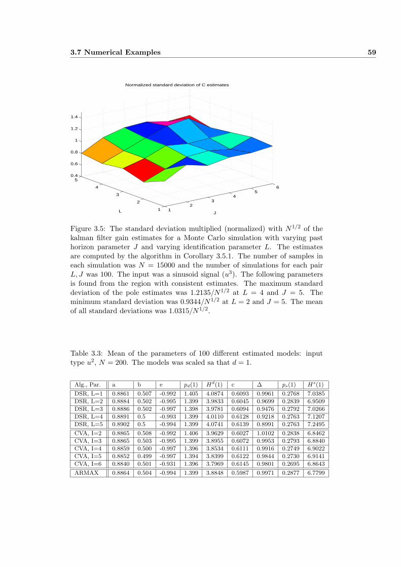
3.7 Numerical Examples 59
12
34
56
1
2
3
4
50.4
0.6
0.8
1
1.2
1.4
L J
Normalized standard deviation of C estimates
Figure 3.5: The standard deviation multiplied (normalized) with N1/2 of thekalman filter gain estimates for a Monte Carlo simulation with varying pasthorizon parameter J and varying identification parameter L. The estimatesare computed by the algorithm in Corollary 3.5.1. The number of samples ineach simulation was N = 15000 and the number of simulations for each pairL, J was 100. The input was a sinusoid signal (u3). The following parametersis found from the region with consistent estimates. The maximum standarddeviation of the pole estimates was 1.2135/N1/2 at L = 4 and J = 5. Theminimum standard deviation was 0.9344/N1/2 at L = 2 and J = 5. The meanof all standard deviations was 1.0315/N1/2.
Table 3.3: Mean of the parameters of 100 different estimated models: inputtype u2, N = 200. The models was scaled sa that d = 1.
Alg., Par. a b e pd(1) Hd(1) c ∆ ps(1) Hs(1)
DSR, L=1 0.8861 0.507 -0.992 1.405 4.0874 0.6093 0.9961 0.2768 7.0385
DSR, L=2 0.8884 0.502 -0.995 1.399 3.9833 0.6045 0.9699 0.2839 6.9509
DSR, L=3 0.8886 0.502 -0.997 1.398 3.9781 0.6094 0.9476 0.2792 7.0266
DSR, L=4 0.8891 0.5 -0.993 1.399 4.0110 0.6128 0.9218 0.2763 7.1207
DSR, L=5 0.8902 0.5 -0.994 1.399 4.0741 0.6139 0.8991 0.2763 7.2495
CVA, I=2 0.8865 0.508 -0.992 1.406 3.9629 0.6027 1.0102 0.2838 6.8462
CVA, I=3 0.8865 0.503 -0.995 1.399 3.8955 0.6072 0.9953 0.2793 6.8840
CVA, I=4 0.8859 0.500 -0.997 1.396 3.8534 0.6111 0.9916 0.2749 6.9022
CVA, I=5 0.8852 0.499 -0.997 1.394 3.8399 0.6122 0.9844 0.2730 6.9141
CVA, I=6 0.8840 0.501 -0.931 1.396 3.7969 0.6145 0.9801 0.2695 6.8643
ARMAX 0.8864 0.504 -0.994 1.399 3.8848 0.5987 0.9971 0.2877 6.7799
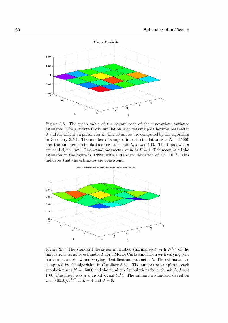
60 Subspace identificatio
12
34
56
1
2
3
4
50.96
0.98
1
1.02
1.04
L J
Mean of F estimates
Figure 3.6: The mean value of the square root of the innovations varianceestimates F for a Monte Carlo simulation with varying past horizon parameterJ and identification parameter L. The estimates are computed by the algorithmin Corollary 3.5.1. The number of samples in each simulation was N = 15000and the number of simulations for each pair L, J was 100. The input was asinusoid signal (u3). The actual parameter value is F = 1. The mean of all theestimates in the figure is 0.9996 with a standard deviation of 7.4 · 10−4. Thisindicates that the estimates are consistent.
12
34
56
1
2
3
4
50
0.2
0.4
0.6
0.8
1
L J
Normalized standard deviation of F estimates
Figure 3.7: The standard deviation multiplied (normalized) with N1/2 of theinnovations variance estimates F for a Monte Carlo simulation with varying pasthorizon parameter J and varying identification parameter L. The estimates arecomputed by the algorithm in Corollary 3.5.1. The number of samples in eachsimulation was N = 15000 and the number of simulations for each pair L, J was100. The input was a sinusoid signal (u1). The minimum standard deviationwas 0.6016/N1/2 at L = 4 and J = 6.
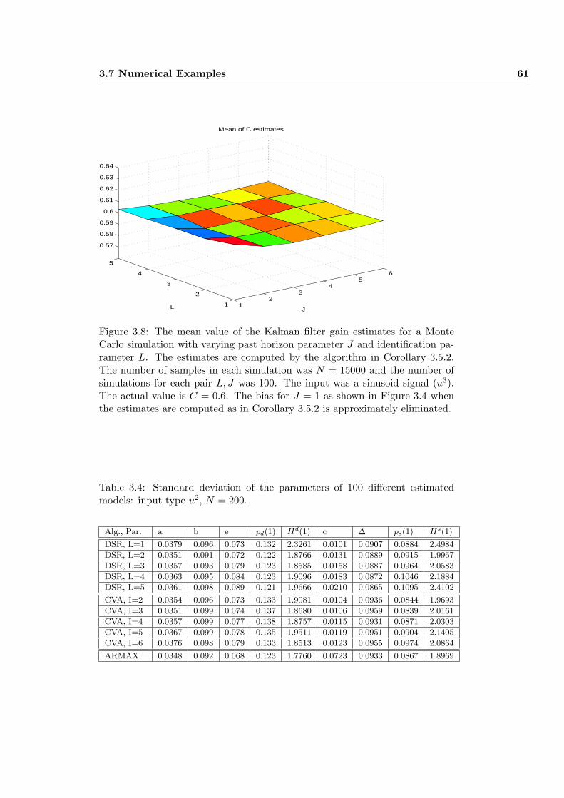
3.7 Numerical Examples 61
12
34
56
1
2
3
4
5
0.57
0.58
0.59
0.6
0.61
0.62
0.63
0.64
L J
Mean of C estimates
Figure 3.8: The mean value of the Kalman filter gain estimates for a MonteCarlo simulation with varying past horizon parameter J and identification pa-rameter L. The estimates are computed by the algorithm in Corollary 3.5.2.The number of samples in each simulation was N = 15000 and the number ofsimulations for each pair L, J was 100. The input was a sinusoid signal (u3).The actual value is C = 0.6. The bias for J = 1 as shown in Figure 3.4 whenthe estimates are computed as in Corollary 3.5.2 is approximately eliminated.
Table 3.4: Standard deviation of the parameters of 100 different estimatedmodels: input type u2, N = 200.
Alg., Par. a b e pd(1) Hd(1) c ∆ ps(1) Hs(1)
DSR, L=1 0.0379 0.096 0.073 0.132 2.3261 0.0101 0.0907 0.0884 2.4984
DSR, L=2 0.0351 0.091 0.072 0.122 1.8766 0.0131 0.0889 0.0915 1.9967
DSR, L=3 0.0357 0.093 0.079 0.123 1.8585 0.0158 0.0887 0.0964 2.0583
DSR, L=4 0.0363 0.095 0.084 0.123 1.9096 0.0183 0.0872 0.1046 2.1884
DSR, L=5 0.0361 0.098 0.089 0.121 1.9666 0.0210 0.0865 0.1095 2.4102
CVA, I=2 0.0354 0.096 0.073 0.133 1.9081 0.0104 0.0936 0.0844 1.9693
CVA, I=3 0.0351 0.099 0.074 0.137 1.8680 0.0106 0.0959 0.0839 2.0161
CVA, I=4 0.0357 0.099 0.077 0.138 1.8757 0.0115 0.0931 0.0871 2.0303
CVA, I=5 0.0367 0.099 0.078 0.135 1.9511 0.0119 0.0951 0.0904 2.1405
CVA, I=6 0.0376 0.098 0.079 0.133 1.8513 0.0123 0.0955 0.0974 2.0864
ARMAX 0.0348 0.092 0.068 0.123 1.7760 0.0723 0.0933 0.0867 1.8969

62 Subspace identificatio
Table 3.5: Mean of the parameters of 100 different estimated models: inputtype u3, N = 500. The models was scaled so that d = 1.
Alg., Par. a b e pd(1) Hd(1) c ∆ ps(1) Hs(1)
DSR, L=1 0.8952 0.493 -1.001 1.392 4.0591 0.6013 1.0006 0.2939 7.0975
DSR, L=2 0.8938 0.494 -1.002 1.390 3.9881 0.5961 0.9879 0.2977 6.9587
DSR, L=3 0.8934 0.493 -1.003 1.389 3.9382 0.6000 0.9784 0.2934 6.9510
DSR, L=4 0.8931 0.493 -1.002 1.389 3.9376 0.6018 0.9695 0.2914 6.9572
DSR, L=5 0.8936 0.493 -1.002 1.390 3.9738 0.6030 0.9612 0.2906 7.0060
CVA, I=2 0.8944 0.493 -1.002 1.391 3.9908 0.5944 1.0047 0.2999 6.9579
CVA, I=3 0.8933 0.492 -1.001 1.389 3.9558 0.5959 0.9998 0.2974 6.9273
CVA, I=4 0.8931 0.492 -1.000 1.389 3.9105 0.5966 0.9992 0.2965 6.8970
CVA, I=5 0.8930 0.492 -1.000 1.389 3.9064 0.5967 0.9986 0.2963 6.8926
CVA, I=6 0.8931 0.491 -1.999 1.389 3.8941 0.5972 0.9977 0.2960 6.8930
ARMAX 0.8936 0.493 -1.002 1.39 3.9354 0.5952 0.9980 0.2983 6.8954
Table 3.6: Standard deviation of the parameters of 100 different estimatedmodels: input type u3, N = 500.
Alg., Par. a b e pd(1) Hd(1) c ∆ ps(1) Hs(1)
DSR, L=1 0.0277 0.066 0.077 0.102 1.6168 0.0409 0.0644 0.0542 1.4790
DSR, L=2 0.0274 0.066 0.075 0.099 1.6257 0.0442 0.0637 0.0580 1.4551
DSR, L=3 0.0268 0.066 0.077 0.099 1.5491 0.0456 0.0638 0.0583 1.4129
DSR, L=4 0.0272 0.066 0.076 0.100 1.5699 0.0470 0.0626 0.0600 1.4067
DSR, L=5 0.0275 0.067 0.076 0.100 1.6054 0.0479 0.0640 0.0609 1.4341
CVA, I=2 0.0269 0.066 0.076 0.100 1.5547 0.0417 0.0653 0.0542 1.4149
CVA, I=3 0.0275 0.066 0.076 0.099 1.5903 0.0431 0.0642 0.0560 1.4462
CVA, I=4 0.0268 0.067 0.075 0.099 1.5164 0.0415 0.0645 0.0532 1.3767
CVA, I=5 0.0267 0.066 0.075 0.099 1.5091 0.0420 0.0645 0.0539 1.3780
CVA, I=6 0.0262 0.067 0.076 0.101 1.5003 0.0433 0.0660 0.0539 1.3668
ARMAX 0.0260 0.066 0.075 0.099 1.5207 0.0421 0.0643 0.0535 1.3581
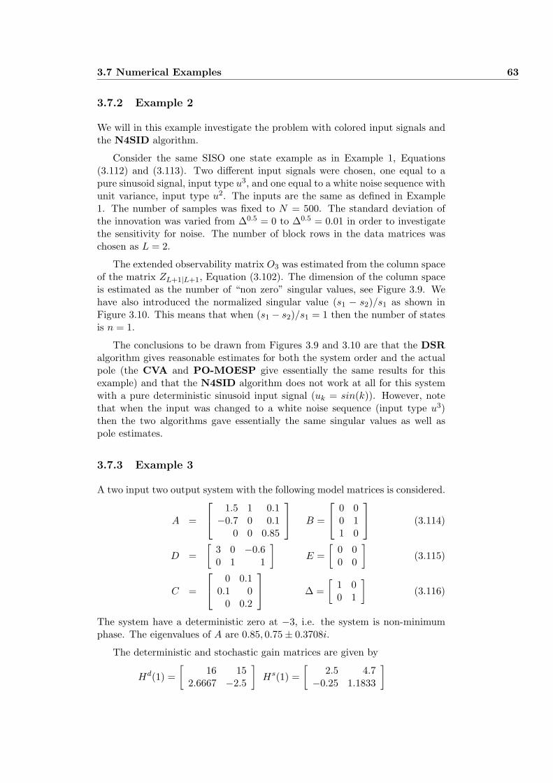
3.7 Numerical Examples 63
3.7.2 Example 2
We will in this example investigate the problem with colored input signals andthe N4SID algorithm.
Consider the same SISO one state example as in Example 1, Equations(3.112) and (3.113). Two different input signals were chosen, one equal to apure sinusoid signal, input type u3, and one equal to a white noise sequence withunit variance, input type u2. The inputs are the same as defined in Example1. The number of samples was fixed to N = 500. The standard deviation ofthe innovation was varied from ∆0.5 = 0 to ∆0.5 = 0.01 in order to investigatethe sensitivity for noise. The number of block rows in the data matrices waschosen as L = 2.
The extended observability matrix O3 was estimated from the column spaceof the matrix ZL+1|L+1, Equation (3.102). The dimension of the column spaceis estimated as the number of “non zero” singular values, see Figure 3.9. Wehave also introduced the normalized singular value (s1 − s2)/s1 as shown inFigure 3.10. This means that when (s1 − s2)/s1 = 1 then the number of statesis n = 1.
The conclusions to be drawn from Figures 3.9 and 3.10 are that the DSRalgorithm gives reasonable estimates for both the system order and the actualpole (the CVA and PO-MOESP give essentially the same results for thisexample) and that the N4SID algorithm does not work at all for this systemwith a pure deterministic sinusoid input signal (uk = sin(k)). However, notethat when the input was changed to a white noise sequence (input type u3)then the two algorithms gave essentially the same singular values as well aspole estimates.
3.7.3 Example 3
A two input two output system with the following model matrices is considered.
A =
1.5 1 0.1−0.7 0 0.1
0 0 0.85
B =
0 00 11 0
(3.114)
D =[
3 0 −0.60 1 1
]E =
[0 00 0
](3.115)
C =
0 0.10.1 0
0 0.2
∆ =
[1 00 1
](3.116)
The system have a deterministic zero at −3, i.e. the system is non-minimumphase. The eigenvalues of A are 0.85, 0.75± 0.3708i.
The deterministic and stochastic gain matrices are given by
Hd(1) =[
16 152.6667 −2.5
]Hs(1) =
[2.5 4.7
−0.25 1.1833
]
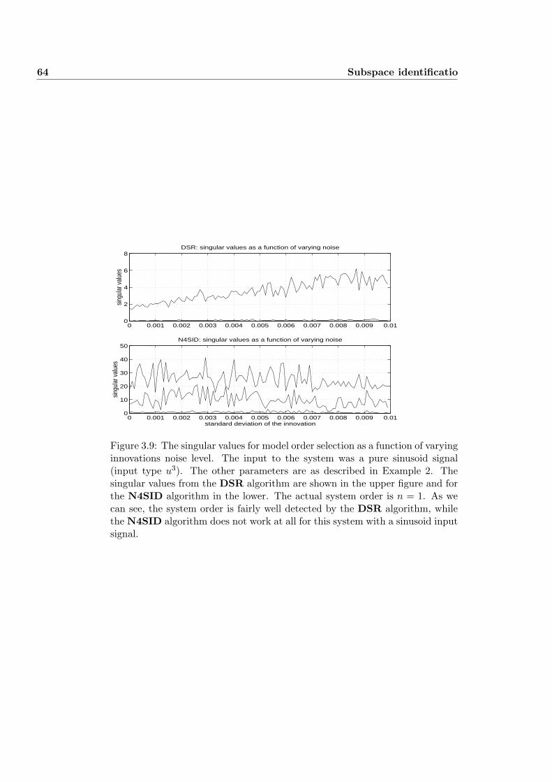
64 Subspace identificatio
0 0.001 0.002 0.003 0.004 0.005 0.006 0.007 0.008 0.009 0.010
2
4
6
8DSR: singular values as a function of varying noise
singu
lar v
alue
s
0 0.001 0.002 0.003 0.004 0.005 0.006 0.007 0.008 0.009 0.010
10
20
30
40
50N4SID: singular values as a function of varying noise
singu
lar v
alue
s
standard deviation of the innovation
Figure 3.9: The singular values for model order selection as a function of varyinginnovations noise level. The input to the system was a pure sinusoid signal(input type u3). The other parameters are as described in Example 2. Thesingular values from the DSR algorithm are shown in the upper figure and forthe N4SID algorithm in the lower. The actual system order is n = 1. As wecan see, the system order is fairly well detected by the DSR algorithm, whilethe N4SID algorithm does not work at all for this system with a sinusoid inputsignal.
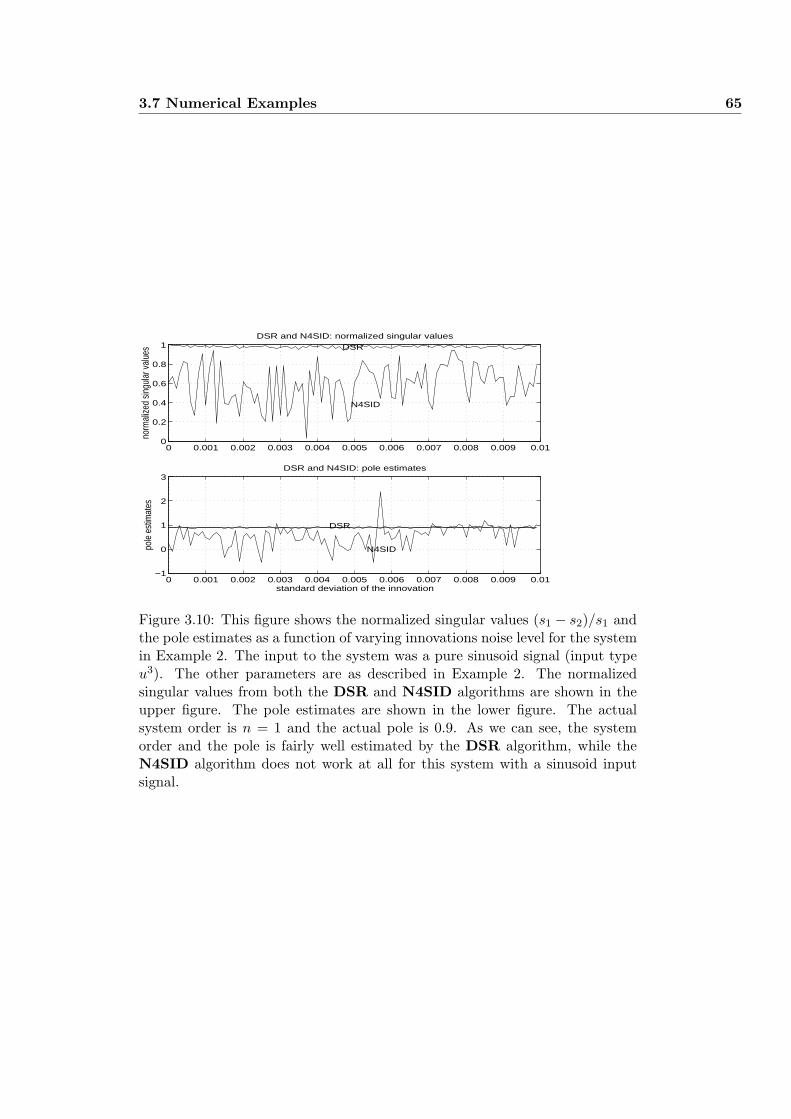
3.7 Numerical Examples 65
0 0.001 0.002 0.003 0.004 0.005 0.006 0.007 0.008 0.009 0.010
0.2
0.4
0.6
0.8
1DSR and N4SID: normalized singular values
norm
alize
d sin
gula
r val
ues
0 0.001 0.002 0.003 0.004 0.005 0.006 0.007 0.008 0.009 0.01−1
0
1
2
3DSR and N4SID: pole estimates
pole
est
imat
es
standard deviation of the innovation
N4SID
N4SID
DSR
DSR
Figure 3.10: This figure shows the normalized singular values (s1 − s2)/s1 andthe pole estimates as a function of varying innovations noise level for the systemin Example 2. The input to the system was a pure sinusoid signal (input typeu3). The other parameters are as described in Example 2. The normalizedsingular values from both the DSR and N4SID algorithms are shown in theupper figure. The pole estimates are shown in the lower figure. The actualsystem order is n = 1 and the actual pole is 0.9. As we can see, the systemorder and the pole is fairly well estimated by the DSR algorithm, while theN4SID algorithm does not work at all for this system with a sinusoid inputsignal.
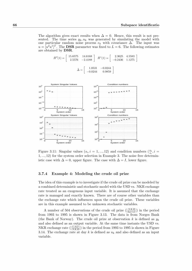
66 Subspace identificatio
The algorithm gives exact results when ∆ = 0. Hence, this result is not pre-sented. The time series yk, uk was generated by simulating the model withone particular random noise process ek with covariance ∆. The input wasu = [u2u1]T . The DSR parameter was fixed to L = 6. The following estimatesare obtained by DSR.
Hd(1) =
[15.6575 14.61682.5576 −2.4188
]Hs(1) =
[2.3625 4.5583
−0.2436 1.1275
]
∆ =
[1.0531 −0.0244
−0.0244 0.9859
]
0 5 10 1510
−2
10−1
100
101
102
System Singular Values
System order0 5 10 15
100
101
102
103
Condition numbers
System order
0 5 10 1510
−15
10−10
10−5
100
105
System Singular Values
System order0 5 10 15
100
105
1010
1015
1020
Condition numbers
System order
Figure 3.11: Singular values (si, i = 1, ..., 12) and condition numbers (s1si
, i =1, ..., 12) for the system order selection in Example 3. The noise free determin-istic case with ∆ = 0, upper figure. The case with ∆ = I, lower figure.
3.7.4 Example 4: Modeling the crude oil prize
The idea of this example is to investigate if the crude oil prize can be modeled bya combined deterministic and stochastic model with the USD vs. NKR exchangerate treated as an exogenous input variable. It is assumed that the exchangerate is managed and exactly known. There are of course other variables thanthe exchange rate which influences upon the crude oil prize. These variablesare in this example assumed to be unknown stochastic variables.
A number of 504 observations of the crude oil prize ([ NKRbarrel ]) in the period
from 1993 to 1995 is shown in Figure 3.13. The data is from Norges Bank(the Bank of Norway). The crude oil prize at observation k is defined as yk
and also defined as an output variable. At the same time instants the USD vs.NKR exchange rate ([ USD
NKR ]) in the period from 1993 to 1995 is shown in Figure3.14. The exchange rate at day k is defined as uk and also defined as an inputvariable.
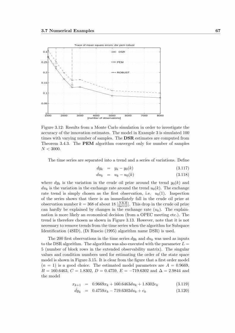
3.7 Numerical Examples 67
1000 2000 3000 4000 5000 6000 7000 80000
0.05
0.1
0.15
0.2
0.25
0.3
[number of observations]
Trace of mean square errors: dsr pem robust
DSR
PEM
ROBUST
Figure 3.12: Results from a Monte Carlo simulation in order to investigate theaccuracy of the innovation estimates. The model in Example 3 is simulated 100times with varying number of samples. The DSR estimates are computed fromTheorem 3.4.3. The PEM algorithm converged only for number of samplesN < 3000.
The time series are separated into a trend and a series of variations. Define
dyk = yk − y0(k) (3.117)duk = uk − u0(k) (3.118)
where dyk is the variation in the crude oil prize around the trend y0(k) andduk is the variation in the exchange rate around the trend u0(k). The exchangerate trend is simply chosen as the first observation, i.e. u0(1). Inspectionof the series shows that there is an immediately fall in the crude oil prize atobservation number k = 368 of about 18 [ NKR
barrel ]. This drop in the crude oil prizecan hardly be explained by changes in the exchange rate (uk). The explain-nation is more likely an economical decision (from a OPEC meeting etc.). Thetrend is therefore chosen as shown in Figure 3.13. However, note that it is notnecessary to remove trends from the time series when the algorithm for SubspaceIdentification (4SID), (Di Ruscio (1995) algorithm name DSR) is used.
The 200 first observations in the time series dyk and duk was used as inputsto the DSR algorithm. The algorithm was also executed with the parameter L =5 (number of block rows in the extended observability matrix). The singularvalues and condition numbers used for estimating the order of the state spacemodel is shown in Figure 3.15. It is clear from the figure that a first order model(n = 1) is a good choice. The estimated model parameters are A = 0.9669,B = 160.6463, C = 1.8302, D = 0.4759, E = −719.6302 and ∆ = 2.9844 andthe model
xk+1 = 0.9669xk + 160.6463duk + 1.8302ek (3.119)dyk = 0.4759xk − 719.6302duk + ek (3.120)
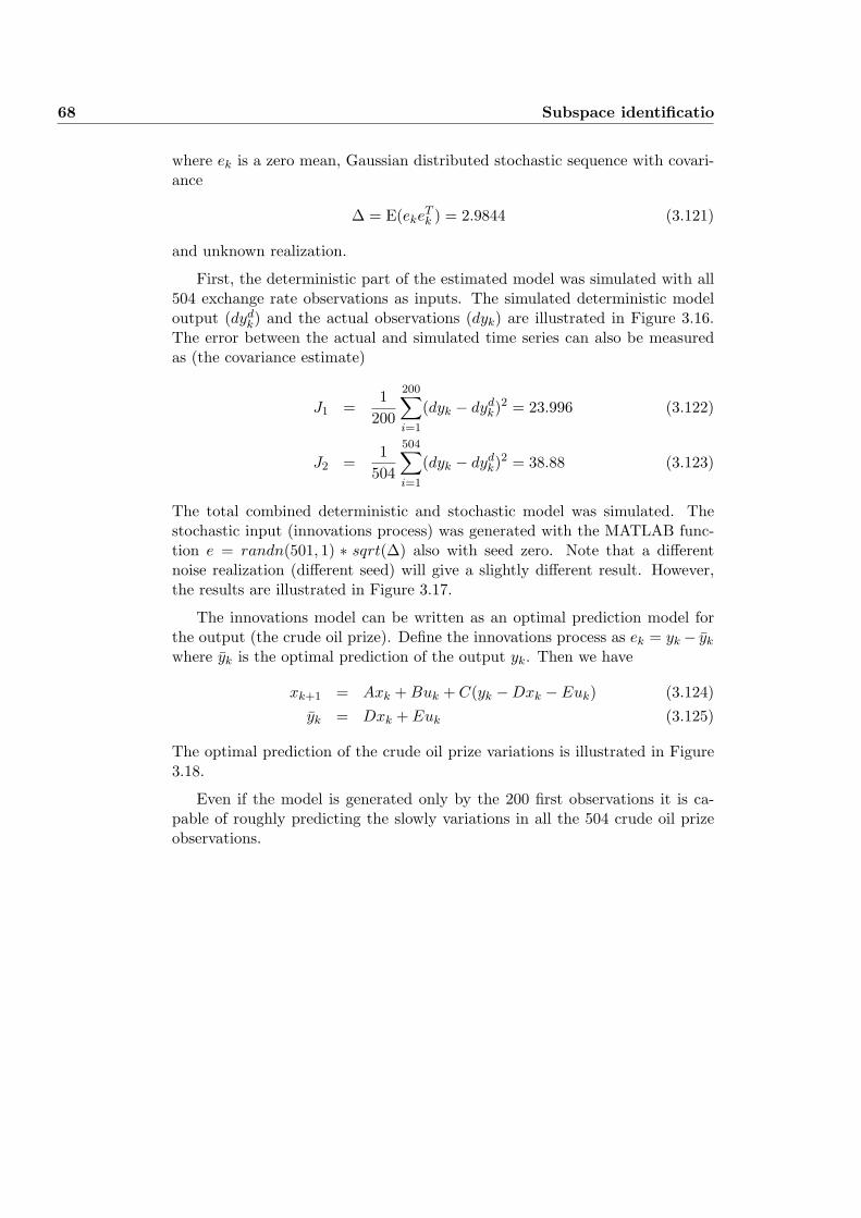
68 Subspace identificatio
where ek is a zero mean, Gaussian distributed stochastic sequence with covari-ance
∆ = E(ekeTk ) = 2.9844 (3.121)
and unknown realization.
First, the deterministic part of the estimated model was simulated with all504 exchange rate observations as inputs. The simulated deterministic modeloutput (dyd
k) and the actual observations (dyk) are illustrated in Figure 3.16.The error between the actual and simulated time series can also be measuredas (the covariance estimate)
J1 =1
200
200∑
i=1
(dyk − dydk)2 = 23.996 (3.122)
J2 =1
504
504∑
i=1
(dyk − dydk)2 = 38.88 (3.123)
The total combined deterministic and stochastic model was simulated. Thestochastic input (innovations process) was generated with the MATLAB func-tion e = randn(501, 1) ∗ sqrt(∆) also with seed zero. Note that a differentnoise realization (different seed) will give a slightly different result. However,the results are illustrated in Figure 3.17.
The innovations model can be written as an optimal prediction model forthe output (the crude oil prize). Define the innovations process as ek = yk − yk
where yk is the optimal prediction of the output yk. Then we have
xk+1 = Axk + Buk + C(yk −Dxk − Euk) (3.124)yk = Dxk + Euk (3.125)
The optimal prediction of the crude oil prize variations is illustrated in Figure3.18.
Even if the model is generated only by the 200 first observations it is ca-pable of roughly predicting the slowly variations in all the 504 crude oil prizeobservations.
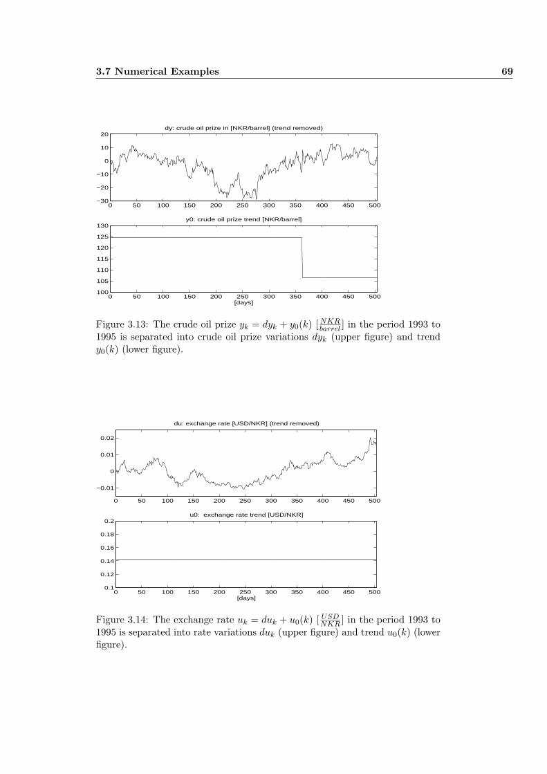
3.7 Numerical Examples 69
0 50 100 150 200 250 300 350 400 450 500−30
−20
−10
0
10
20dy: crude oil prize in [NKR/barrel] (trend removed)
0 50 100 150 200 250 300 350 400 450 500100
105
110
115
120
125
130
[days]
y0: crude oil prize trend [NKR/barrel]
Figure 3.13: The crude oil prize yk = dyk + y0(k) [ NKRbarrel ] in the period 1993 to
1995 is separated into crude oil prize variations dyk (upper figure) and trendy0(k) (lower figure).
0 50 100 150 200 250 300 350 400 450 500
−0.01
0
0.01
0.02
du: exchange rate [USD/NKR] (trend removed)
0 50 100 150 200 250 300 350 400 450 5000.1
0.12
0.14
0.16
0.18
0.2
[days]
u0: exchange rate trend [USD/NKR]
Figure 3.14: The exchange rate uk = duk + u0(k) [ USDNKR ] in the period 1993 to
1995 is separated into rate variations duk (upper figure) and trend u0(k) (lowerfigure).
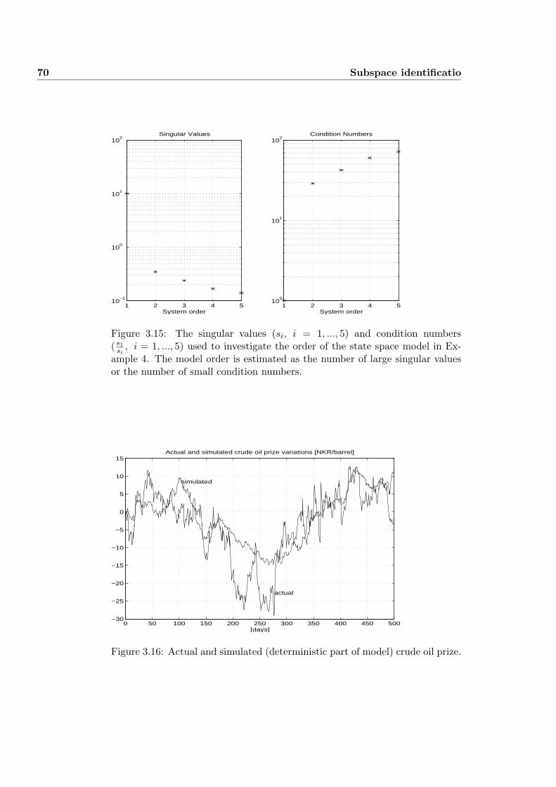
70 Subspace identificatio
1 2 3 4 510
−1
100
101
102
Singular Values
System order1 2 3 4 5
100
101
102
Condition Numbers
System order
Figure 3.15: The singular values (si, i = 1, ..., 5) and condition numbers( s1
si, i = 1, ..., 5) used to investigate the order of the state space model in Ex-
ample 4. The model order is estimated as the number of large singular valuesor the number of small condition numbers.
0 50 100 150 200 250 300 350 400 450 500−30
−25
−20
−15
−10
−5
0
5
10
15Actual and simulated crude oil prize variations [NKR/barrel]
[days]
simulated
actual
Figure 3.16: Actual and simulated (deterministic part of model) crude oil prize.

3.7 Numerical Examples 71
0 50 100 150 200 250 300 350 400 450 500−30
−25
−20
−15
−10
−5
0
5
10
15
20
Actual and simulated crude oil prize variazions [NKR/barrel]
simulated
actual
Figure 3.17: Actual and simulated (combined deterministic and stochasticmodel) crude oil prize. This model was generated from the 200 first samples ofthe input output samples, only. The algorithm parameter was L = 5.
0 50 100 150 200 250 300 350 400 450 500−30
−20
−10
0
10
Actual and optimal prediction of crude oil prize variations [NKR/barrel]
[days]
0 50 100 150 200 250 300 350 400 450 500−10
−5
0
5
10Difference between actual and optimal prediction of crude oil prize
[days]
Figure 3.18: Actual and simulated optimal prediction of the crude oil prize isshown in the upper part of the figure. The difference between the actual andthe optimal prediction of the crude oil prize is shown in the lower part of thefigure. This model was generated from the 200 first samples of the input outputsamples, only. The algorithm parameter was L = 5.
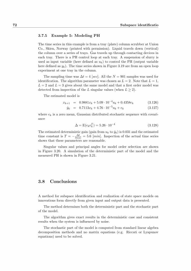
72 Subspace identificatio
3.7.5 Example 5: Modeling PH
The time series in this example is from a tray (plate) column scrubber at UnionCo., Skien, Norway (printed with permission). Liquid travels down (vertical)the column over a series of trays. Gas travels up through contacting devices ineach tray. There is a PH control loop at each tray. A suspension of slurry isused as input variable (here defined as uk) to control the PH (output variablehere defined as yk). The time series shown in Figure 3.19 are from an open loopexperiment at one tray in the column.
The sampling time was ∆t = 4 [sec]. All the N = 901 samples was used foridentification. The algorithm parameter was chosen as L = 2. Note that L = 1,L = 2 and L = 3 gives about the same model and that a first order model wasdetected from inspection of the L singular values (when L ≥ 2).
The estimated model is
xk+1 = 0.9881xk + 5.09 · 10−4uk + 0.4358ek (3.126)yk = 0.7113xk + 4.76 · 10−5uk + ek (3.127)
where ek is a zero mean, Gaussian distributed stochastic sequence with covari-ance
∆ = E(ekeTk ) = 5.26 · 10−4 (3.128)
The estimated deterministic gain (gain from uk to yk) is 0.031 and the estimatedtime constant is T = − ∆t
ln(a) = 5.6 [min]. Inspection of the actual time seriesshows that these parameters are reasonable.
Singular values and principal angles for model order selection are shownin Figure 3.20. A simulation of the deterministic part of the model and themeasured PH is shown in Figure 3.21.
3.8 Conclusions
A method for subspace identification and realization of state space models oninnovations form directly from given input and output data is presented.
The method determines both the deterministic part and the stochastic partof the model.
The algorithm gives exact results in the deterministic case and consistentresults when the system is influenced by noise.
The stochastic part of the model is computed from standard linear algebradecomposition methods and no matrix equations (e.g. Riccati or Lyapunovequations) need to be solved.
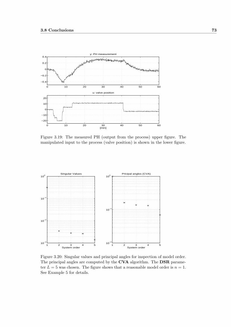
3.8 Conclusions 73
0 10 20 30 40 50 60
−0.4
−0.2
0
0.2
0.4y: PH measurement
0 10 20 30 40 50 60
−20
−10
0
10
20
[min]
u: valve position
Figure 3.19: The measured PH (output from the process) upper figure. Themanipulated input to the process (valve position) is shown in the lower figure.
1 2 3 4 510
−3
10−2
10−1
100
Singular Values
System order1 2 3 4 5
10−2
10−1
100
Pricipal angles (CVA)
System order
Figure 3.20: Singular values and principal angles for inspection of model order.The principal angles are computed by the CVA algorithm. The DSR parame-ter L = 5 was chosen. The figure shows that a reasonable model order is n = 1.See Example 5 for details.
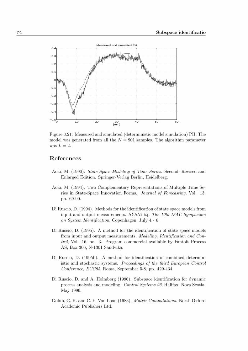
74 Subspace identificatio
0 10 20 30 40 50 60−0.5
−0.4
−0.3
−0.2
−0.1
0
0.1
0.2
0.3
0.4
[min]
Measured and simulated PH
Figure 3.21: Measured and simulated (deterministic model simulation) PH. Themodel was generated from all the N = 901 samples. The algorithm parameterwas L = 2.
References
Aoki, M. (1990). State Space Modeling of Time Series. Second, Revised andEnlarged Edition. Springer-Verlag Berlin, Heidelberg.
Aoki, M. (1994). Two Complementary Representations of Multiple Time Se-ries in State-Space Innovation Forms. Journal of Forecasting, Vol. 13,pp. 69-90.
Di Ruscio, D. (1994). Methods for the identification of state space models frominput and output measurements. SYSID 94, The 10th IFAC Symposiumon System Identification, Copenhagen, July 4 - 6.
Di Ruscio, D. (1995). A method for the identification of state space modelsfrom input and output measurements. Modeling, Identification and Con-trol, Vol. 16, no. 3. Program commercial available by Fantoft ProcessAS, Box 306, N-1301 Sandvika.
Di Ruscio, D. (1995b). A method for identification of combined determin-istic and stochastic systems. Proceedings of the third European ControlConference, ECC95, Roma, September 5-8, pp. 429-434.
Di Ruscio, D. and A. Holmberg (1996). Subspace identification for dynamicprocess analysis and modeling. Control Systems 96, Halifax, Nova Scotia,May 1996.
Golub, G. H. and C. F. Van Loan (1983). Matrix Computations. North OxfordAcademic Publishers Ltd.

3.8 Conclusions 75
Larimore, W. E. (1983). System identification, reduced order filtering andmodeling via canonical variate analysis. Proc. of the American ControlConference, San Francisco, USA, pp. 445-451.
Larimore, W. E. (1990). Canonical Variate Analysis in Identification, Filteringand Adaptive Control. Proc. of the 29th Conference on Decision andControl, Honolulu, Hawaii, December 1990, pp. 596-604.
Ljung, L. (1991). System Identification Toolbox. The Mathworks, Inc.
Faurre, P. L. (1976). Stochastic realization algorithms. In: System Identifica-tion: Advances and Case Studies, (eds. R. K. Mehra and D. G. Lainiotis),Academic Press.
Kalman, R. E., P. L. Falb and M. A. Arbib (1969). Topics in mathematicalsystem theory. McGraw-Hill Book Company.
Kung, S. Y. (1978). A new identification and Model Reduction Algorithm viaSingular Value Decomposition. Conf. on Circuits, Systems and Comput-ers, Pacific Grove, CA, November 1978, pp. 705-714.
Moore, B. C. (1981). Principal Component Analysis in Linear Systems: Con-trollability, Observability, and Model Reduction. IEEE Trans. on Auto-matic Control, Vol. AC-26, pp. 17-31.
Van Overschee, P. and B. De Moor (1994). N4SID: Subspace Algorithms forthe Identification of Combined Deterministic Stochastic Systems. Auto-matica, vol. 30, No. 1, pp.75-94.
Van Overschee, P. (1995). Subspace Identification: theory-implementation-application. PhD thesis, Katholieke Universiteit Leuven, Belgium.
Van Overschee, P. and B. De Moor (1995). A Unifying Theorem for ThreeSubspace System Identification Algorithms. Automatica, vol. 31, No. 12,pp. 1853-1864.
Verhagen, M. (1994). Identification of the deterministic part of MIMO statespace models given on innovations form from input output data. Auto-matica, vol. 30, No. 1, pp. 61-74.
Viberg, M. (1995). Subspace-Based Methods for the Identification of LinearTime-invariant Systems. Automatica, vol. 31, No. 12, pp. 1835-1851.

76 Subspace identificatio
Corrections
1. Index error in the matrices with zeroes on the right hand side (rhs) ofEquation (3.46).In the third rhs term, change 0Lm×(k+L+1−J)r to 0(L+1)m×(k+L+1−J)r. Inthe fifth rhs term, change 0Lm×(k+L+1−J)r to 0(L+1)m×(k+L+1−J)m. Theerror is changed.
2. Index error on the right hand side of Equation (3.49). Change E0|L+1 toE0|J . The error is changed.
3. Index error on the right hand side of Equation (3.51). Change E0|L+1 toE0|J . The error is changed.
4. Index error on the right hand side of Equation (3.52). Change E0|L+1 toE0|J . The error is changed.
5. The matrix U⊥L+1|L+1 is missing on the right hand side in Equation (3.109).
The column weighting matrix Wc in the N4SID algorithm should be
Wc = U⊥L+1|L+1W
T1 (W1U
⊥L+1|L+1W
T1 )−1W1
The error is changed.
Chapter 4
On the DSR algorithm
4.1 Introduction
The theory of subspace identification (SID) methods will be presented in gen-eral. The theory and application of one particular SID method will be presentedin some detail.
A SID method can be viewed as a realization based approach to estimat-ing state space models from input and output data. This is a most effectiveand useful method, in particular for multivariable input and output (combineddeterministic and stochastic) systems.
A lower Left Q-orthogonal (LQ) decomposition is often used in subspaceidentification methods in order to compute certain projection matrices andsubspaces of the known data matrices and to estimate the system order andthe extended observability matrix of the dynamic system.
The dynamics of the system can be extracted from the column space R(Z)of one particular projected matrix Z which is computed from the input andoutput data matrices Y , U and a method for computing subspaces, e.g., LQdecomposition, singular value decomposition. An alternative method (to com-pute the projection matrices, subspaces and the column space R(Z)) whichis based on the Partial Least Squares (PLS) method (decomposition) is alsopresented.
Two examples are presented in order to compare different SID methods.First: a Monte Carlo simulation experiment of a MIMO system is presented inorder to compare the numerically reliability of one particular subspace methodwith two other subspace methods presented in the literature.
Second: a real world example from the pulp and paper industry is presentedin order to compare the quality of the methods. For this example there are threeinput variables in the U data matrix and two output variables in the Y datamatrix. The data was collected from an experiment design. The quality ofthe different models and validation aspects are addressed. The estimated state

78 On the DSR algorithm
space model is then used in a model predictive control strategy. Simulationresults are presented.
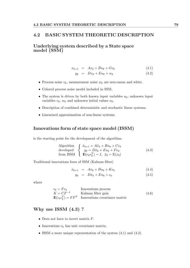
4.2 BASIC SYSTEM THEORETIC DESCRIPTION 79
4.2 BASIC SYSTEM THEORETIC DESCRIPTION
Underlying system described by a State spacemodel (SSM)
xk+1 = Axk + Buk + Gvk (4.1)yk = Dxk + Euk + wk (4.2)
• Process noise vk, measurement noise wk are zero-mean and white.
• Colored process noise model included in SSM.
• The system is driven by both known input variables uk, unknown inputvariables vk, wk and unknown initial values x0.
• Description of combined deterministic and stochastic linear systems.
• Linearized approximation of non-linear systems.
Innovations form of state space model (ISSM)
is the starting point for the development of the algorithm.
Algorithmdevelopedfrom ISSM
xk+1 = Axk + Buk + Cek
yk = Dxk + Euk + Fek
E(ekeTk ) = I, x0 = E(x0)
(4.3)
Traditional innovations form of SSM (Kalman filter)
xk+1 = Axk + Buk + Kεk (4.4)yk = Dxk + Euk + εk (4.5)
where
εk = Fek Innovations processK = CF−1 Kalman filter gainE(εkε
Tk ) = FF T Innovations covariance matrix
(4.6)
Why use ISSM (4.3) ?
• Does not have to invert matrix F .
• Innovations ek has unit covariance matrix.
• ISSM a more unique representation of the system (4.1) and (4.2).

80 On the DSR algorithm
4.3 PROBLEM DESCRIPTION
From known system input and output data
uk ∀ k = 1, 2, ..., Nyk ∀ k = 1, 2, ..., N
}Known data
find the system order n, the initial state vector x0 and matrices in the ISSM(up to within a similarity transformation)
A B CD E F x0
{find system order andmatrices from known data
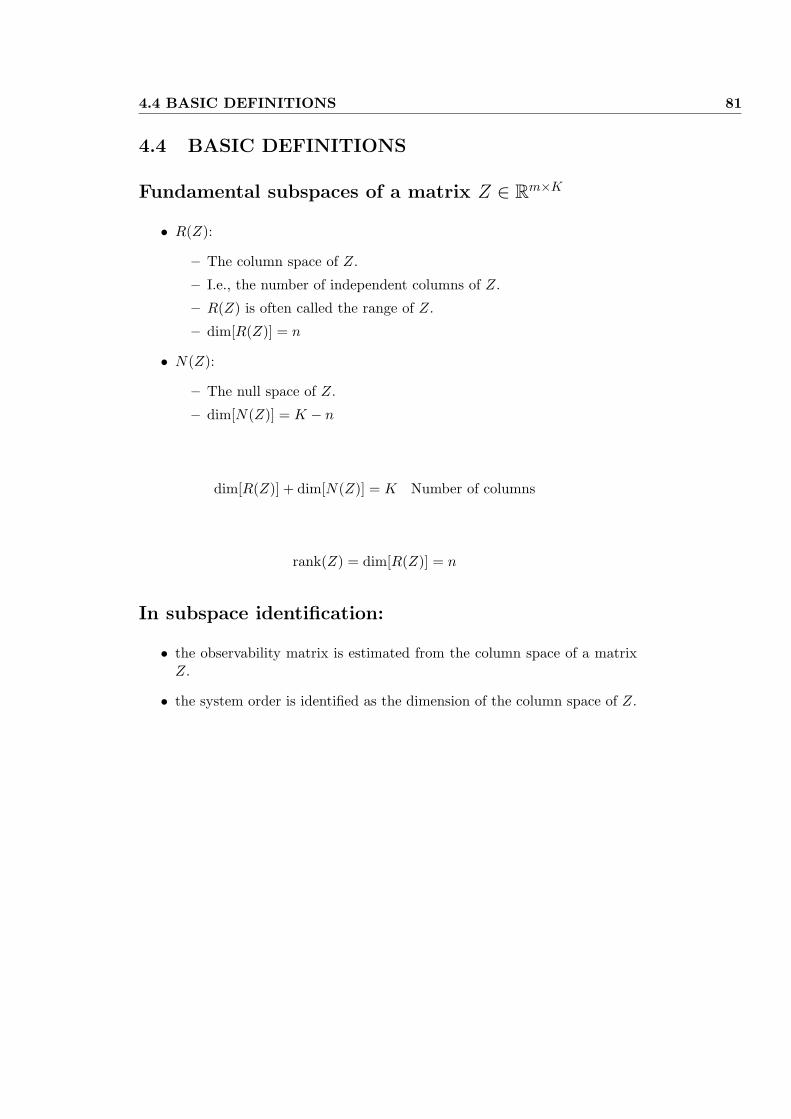
4.4 BASIC DEFINITIONS 81
4.4 BASIC DEFINITIONS
Fundamental subspaces of a matrix Z ∈ Rm×K
• R(Z):
– The column space of Z.
– I.e., the number of independent columns of Z.
– R(Z) is often called the range of Z.
– dim[R(Z)] = n
• N(Z):
– The null space of Z.
– dim[N(Z)] = K − n
dim[R(Z)] + dim[N(Z)] = K Number of columns
rank(Z) = dim[R(Z)] = n
In subspace identification:
• the observability matrix is estimated from the column space of a matrixZ.
• the system order is identified as the dimension of the column space of Z.
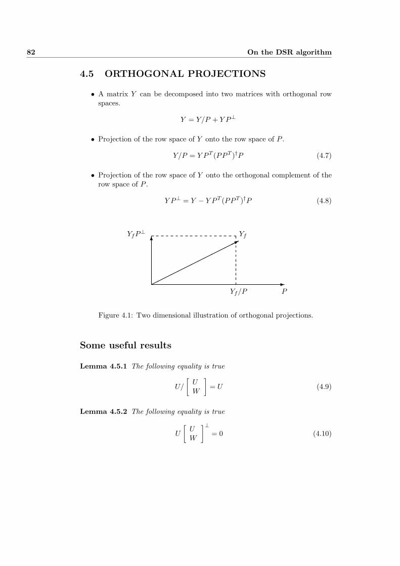
82 On the DSR algorithm
4.5 ORTHOGONAL PROJECTIONS
• A matrix Y can be decomposed into two matrices with orthogonal rowspaces.
Y = Y/P + Y P⊥
• Projection of the row space of Y onto the row space of P .
Y/P = Y P T (PP T )†P (4.7)
• Projection of the row space of Y onto the orthogonal complement of therow space of P .
Y P⊥ = Y − Y P T (PP T )†P (4.8)
-©©©©©©©©©©©©©©*6YfYfP⊥
Yf/P P
Figure 4.1: Two dimensional illustration of orthogonal projections.
Some useful results
Lemma 4.5.1 The following equality is true
U/
[UW
]= U (4.9)
Lemma 4.5.2 The following equality is true
U
[UW
]⊥= 0 (4.10)
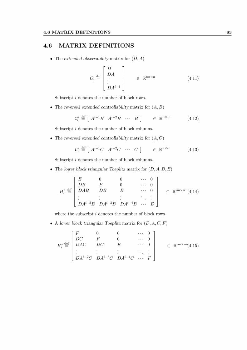
4.6 MATRIX DEFINITIONS 83
4.6 MATRIX DEFINITIONS
• The extended observability matrix for (D, A)
Oidef=
DDA...DAi−1
∈ Rim×n (4.11)
Subscript i denotes the number of block rows.
• The reversed extended controllability matrix for (A,B)
Cdi
def=[
Ai−1B Ai−2B · · · B] ∈ Rn×ir (4.12)
Subscript i denotes the number of block columns.
• The reversed extended controllability matrix for (A,C)
Csi
def=[
Ai−1C Ai−2C · · · C] ∈ Rn×ir (4.13)
Subscript i denotes the number of block columns.
• The lower block triangular Toeplitz matrix for (D, A,B,E)
Hdi
def=
E 0 0 · · · 0DB E 0 · · · 0DAB DB E · · · 0...
......
. . ....
DAi−2B DAi−3B DAi−4B · · · E
∈ Rim×ir (4.14)
where the subscript i denotes the number of block rows.
• A lower block triangular Toeplitz matrix for (D, A,C, F )
Hsi
def=
F 0 0 · · · 0DC F 0 · · · 0DAC DC E · · · 0...
......
. . ....
DAi−2C DAi−3C DAi−4C · · · F
∈ Rim×im(4.15)
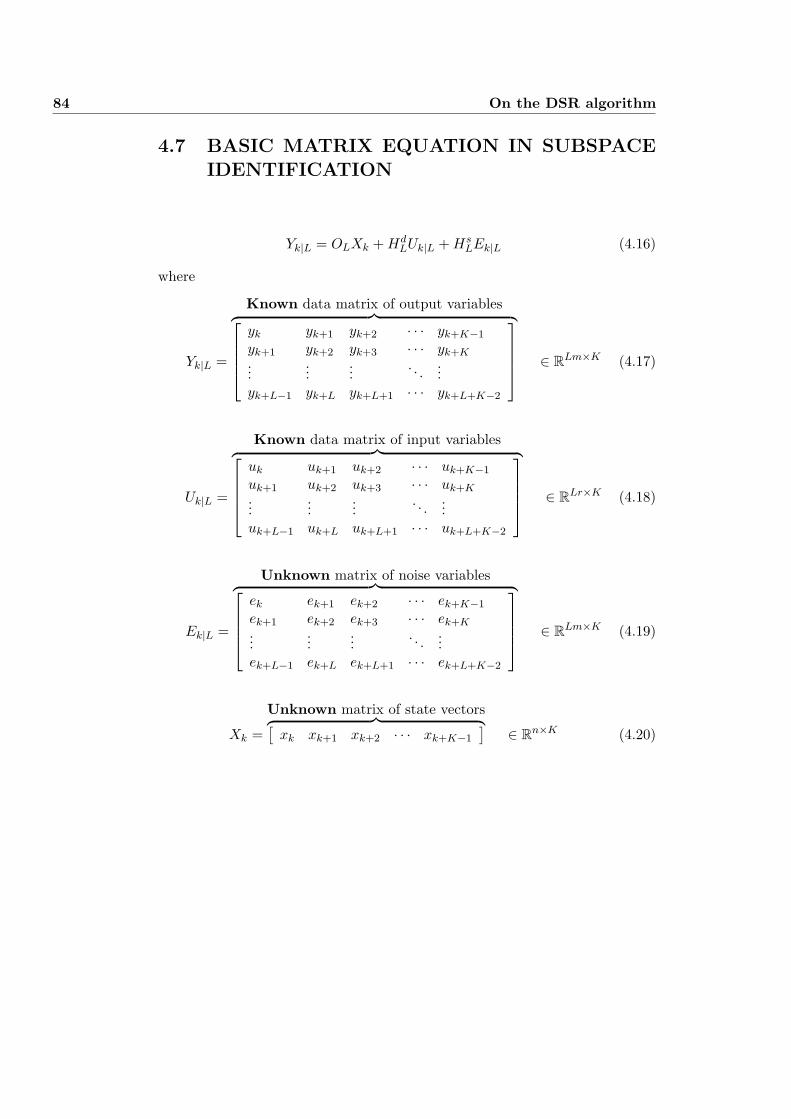
84 On the DSR algorithm
4.7 BASIC MATRIX EQUATION IN SUBSPACEIDENTIFICATION
Yk|L = OLXk + HdLUk|L + Hs
LEk|L (4.16)
where
Yk|L =
Known data matrix of output variables︷ ︸︸ ︷
yk yk+1 yk+2 · · · yk+K−1
yk+1 yk+2 yk+3 · · · yk+K...
......
. . ....
yk+L−1 yk+L yk+L+1 · · · yk+L+K−2
∈ RLm×K (4.17)
Uk|L =
Known data matrix of input variables︷ ︸︸ ︷
uk uk+1 uk+2 · · · uk+K−1
uk+1 uk+2 uk+3 · · · uk+K...
......
. . ....
uk+L−1 uk+L uk+L+1 · · · uk+L+K−2
∈ RLr×K (4.18)
Ek|L =
Unknown matrix of noise variables︷ ︸︸ ︷
ek ek+1 ek+2 · · · ek+K−1
ek+1 ek+2 ek+3 · · · ek+K...
......
. . ....
ek+L−1 ek+L ek+L+1 · · · ek+L+K−2
∈ RLm×K (4.19)
Xk =
Unknown matrix of state vectors︷ ︸︸ ︷[xk xk+1 xk+2 · · · xk+K−1
] ∈ Rn×K (4.20)
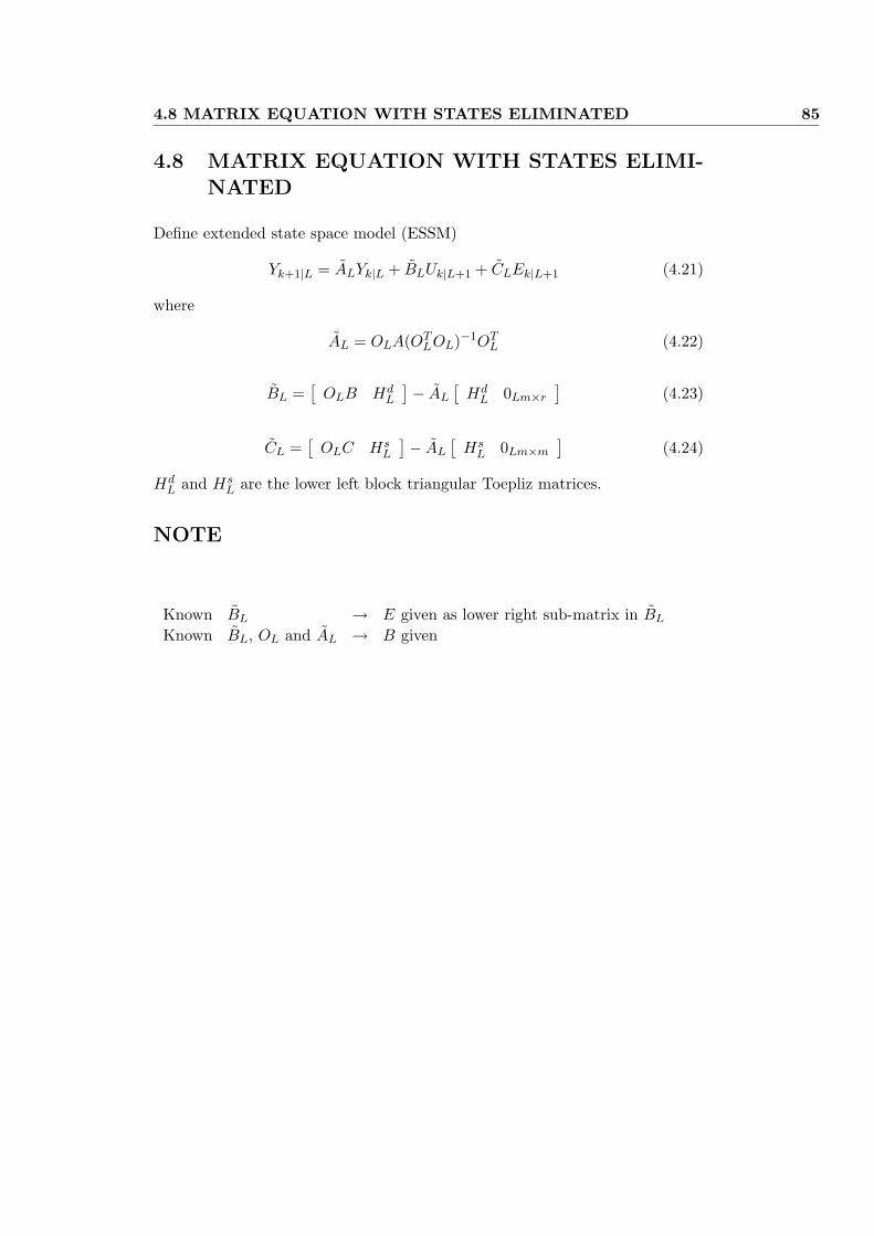
4.8 MATRIX EQUATION WITH STATES ELIMINATED 85
4.8 MATRIX EQUATION WITH STATES ELIMI-NATED
Define extended state space model (ESSM)
Yk+1|L = ALYk|L + BLUk|L+1 + CLEk|L+1 (4.21)
where
AL = OLA(OTLOL)−1OT
L (4.22)
BL =[
OLB HdL
]− AL
[Hd
L 0Lm×r
](4.23)
CL =[
OLC HsL
]− AL
[Hs
L 0Lm×m
](4.24)
HdL and Hs
L are the lower left block triangular Toepliz matrices.
NOTE
Known BL → E given as lower right sub-matrix in BL
Known BL, OL and AL → B given
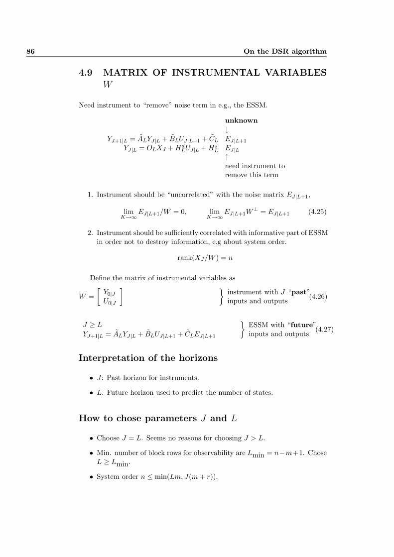
86 On the DSR algorithm
4.9 MATRIX OF INSTRUMENTAL VARIABLESW
Need instrument to “remove” noise term in e.g., the ESSM.
unknown↓
YJ+1|L = ALYJ |L + BLUJ |L+1 + CL EJ |L+1
YJ |L = OLXJ + HdLUJ |L + Hs
L EJ |L↑need instrument toremove this term
1. Instrument should be “uncorrelated” with the noise matrix EJ |L+1,
limK→∞
EJ |L+1/W = 0, limK→∞
EJ |L+1W⊥ = EJ |L+1 (4.25)
2. Instrument should be sufficiently correlated with informative part of ESSMin order not to destroy information, e.g about system order.
rank(XJ/W ) = n
Define the matrix of instrumental variables as
W =[
Y0|JU0|J
] }instrument with J “past”inputs and outputs
(4.26)
J ≥ L
YJ+1|L = ALYJ |L + BLUJ |L+1 + CLEJ |L+1
}ESSM with “future”inputs and outputs
(4.27)
Interpretation of the horizons
• J : Past horizon for instruments.
• L: Future horizon used to predict the number of states.
How to chose parameters J and L
• Choose J = L. Seems no reasons for choosing J > L.
• Min. number of block rows for observability are Lmin = n−m+1. ChoseL ≥ Lmin.
• System order n ≤ min(Lm, J(m + r)).
4.10 Subspace identification of OL: autonomous systems 87
4.10 Subspace identification of OL: autonomous sys-tems
Consider the matrix equation
Zk|L = OLXk ∈ RLm×K (4.28)
Assumptions
• Data matrix Zk|L known.
• The pair (D,A) observable.
• rank(Xk) = n.
Column space of product
• The column space of OLXk is contained in the column space of OL.
R(OLXk) ⊆ R(OL) (4.29)
Sylvesters inequality gives
rank(OL) + rank(Xk)− n ≤ rank(Zk|L) ≤ min{rank(OL), rank(Xk)} (4.30)
Conclusions
• The column space of Zk|L coincide with the column space of OL.
R(Zk|L) = R(OL) (4.31)
• The rank of Zk|L (which is equal to the dimension of the column space)is equal to the number of states n.
rank(Zk|L) = dim[R(Zk|L)] = n (4.32)
• Can estimate both the system order n and the extended observabilitymatrix OL from the matrix Zk|L.
88 On the DSR algorithm
4.11 Subspace identification of OL: deterministic sys-tems
Deterministic SSM can be written as the matrix equation
Yk|L = OLXk + HdLUk|L (4.33)
• Data-matrices Yk|L and Uk|L are known.
Results
Zk|Ldef= Yk|LU⊥
k|L = OLXkU⊥k|L (4.34)
and
rank(Zk|L) = n if rank(XkU⊥k|L) = n (4.35)
• XkU⊥k|L loose rank below n ?
Analysis
A matrix Xk can be decomposed into two matrices with orthogonal row spaces.
Xk = Xk/Uk|L + XkU⊥k|L
-©©©©©©©©©©©©©©*6XkXkU
⊥k|L
Xk/Uk|L Uk|L
• Xk/Uk|L: Projection of the row space of Xk on the row space of Uk|L.
• XkU⊥k|L: Projection of the row space of Xk onto the orthogonal comple-
ment of the row space of Uk|L.
4.12 Subspace identification of OL+1: “general” case 89
Conclusion
rank(XkU⊥k|L) = n if Xk 6= Uk|L (4.36)
4.12 Subspace identification of OL+1: “general” case
Theorem 4.12.1 (Realization of the extended observability matrix OL+1)
Define from the known data
ZJ |L+1def= (YJ |L+1/
UJ |L+1
U0|JY0|J
)U⊥
J |L+1, (4.37)
ZJ |L+1 is related to the extended observability matrix as
ZJ |L+1 = OL+1XaJ (4.38)
where
XaJ = XJ/
UJ |L+1
U0|JY0|J
U⊥
J |L+1 =[
AJ CdJ Cs
J
]
X0/
UJ |L+1
U0|JY0|J
U0|J
E0|J/
UJ |L+1
U0|JY0|J
U⊥J |L+1
• The column space of ZJ |L+1 coincides with column space of OL+1.
• The system order n is given as the dimension of the column space.
90 On the DSR algorithm
4.13 BASIC PROJECTIONS IN THE DSR ALGO-RITHM
“Autonomous system” for system dynamics, A and D
ZJ |L+1 = OL+1XaJ (4.39)
ZJ+1|L = ALZJ |L (4.40)
where
ZJ |L+1def= (YJ |L+1/
UJ |L+1
U0|JY0|J
)U⊥
J |L+1 (4.41)
Hence,
(A, D) = arg minA,D
‖ ZJ+1|L − ALZJ |L ‖2F (4.42)
“Deterministic system” for B and E
ZdJ+1|L = ALZd
J |L + BLUJ |L+1 (4.43)
where
ZdJ |L+1
def= YJ |L+1/
UJ |L+1
U0|JY0|J
(4.44)
Hence,
(B,E) = arg minB,E
‖ ZdJ+1|L − ALZd
J |L − BLUJ |L+1 ‖2F (4.45)
“Stochastic system” for C and F
ZsJ+1|L = ALZs
J |L + CLEJ |L+1 (4.46)
where
ZsJ |L+1
def= YJ |L+1
UJ |L+1
U0|JY0|J
⊥
(4.47)
Hence,
(C, F ) = arg minC,F
‖ ZsJ+1|L − ALZs
J |L − CLEJ |L+1 ‖2F (4.48)
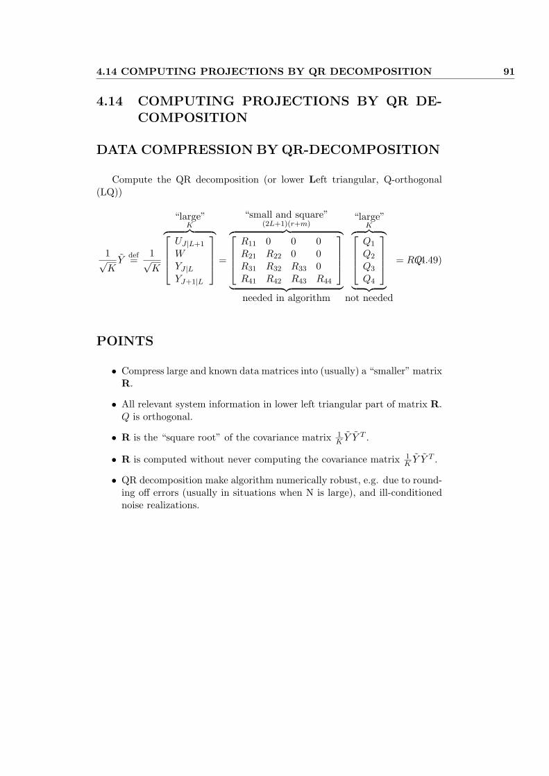
4.14 COMPUTING PROJECTIONS BY QR DECOMPOSITION 91
4.14 COMPUTING PROJECTIONS BY QR DE-COMPOSITION
DATA COMPRESSION BY QR-DECOMPOSITION
Compute the QR decomposition (or lower Left triangular, Q-orthogonal(LQ))
1√K
Ydef=
1√K
“large”K︷ ︸︸ ︷
UJ |L+1
WYJ |LYJ+1|L
=
“small and square”(2L+1)(r+m)︷ ︸︸ ︷
R11 0 0 0R21 R22 0 0R31 R32 R33 0R41 R42 R43 R44
︸ ︷︷ ︸needed in algorithm
“large”K︷ ︸︸ ︷
Q1
Q2
Q3
Q4
︸ ︷︷ ︸not needed
= RQ(4.49)
POINTS
• Compress large and known data matrices into (usually) a “smaller” matrixR.
• All relevant system information in lower left triangular part of matrix R.Q is orthogonal.
• R is the “square root” of the covariance matrix 1K Y Y T .
• R is computed without never computing the covariance matrix 1K Y Y T .
• QR decomposition make algorithm numerically robust, e.g. due to round-ing off errors (usually in situations when N is large), and ill-conditionednoise realizations.
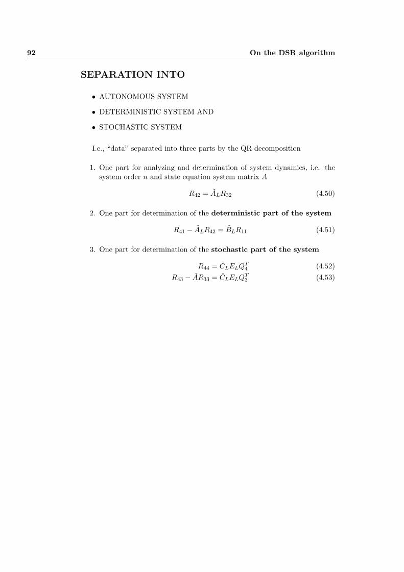
92 On the DSR algorithm
SEPARATION INTO
• AUTONOMOUS SYSTEM
• DETERMINISTIC SYSTEM AND
• STOCHASTIC SYSTEM
I.e., “data” separated into three parts by the QR-decomposition
1. One part for analyzing and determination of system dynamics, i.e. thesystem order n and state equation system matrix A
R42 = ALR32 (4.50)
2. One part for determination of the deterministic part of the system
R41 − ALR42 = BLR11 (4.51)
3. One part for determination of the stochastic part of the system
R44 = CLELQT4 (4.52)
R43 − AR33 = CLELQT3 (4.53)
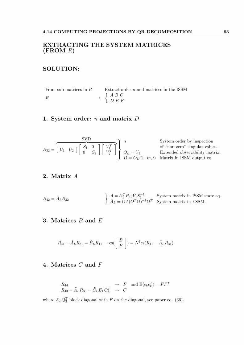
4.14 COMPUTING PROJECTIONS BY QR DECOMPOSITION 93
EXTRACTING THE SYSTEM MATRICES(FROM R)
SOLUTION:
From sub-matrices in R Extract order n and matrices in the ISSM
R →{
A B CD E F
1. System order: n and matrix D
R32 =
SVD︷ ︸︸ ︷[
U1 U2
] [S1 00 S2
] [V T
1
V T2
]
n System order by inspectionof “non zero” singular values.
OL = U1 Extended observability matrix.D = OL(1 : m, :) Matrix in ISSM output eq.
2. Matrix A
R42 = ALR32
}A = UT
1 R42V1S−11 System matrix in ISSM state eq.
AL = OA(OT O)−1OT System matrix in ESSM.
3. Matrices B and E
R41 − ALR31 = BLR11 → cs([
BE
]) = N †cs(R41 − ALR31)
4. Matrices C and F
R44 → F and E(εkεTk ) = FF T
R43 − ALR33 = CLELQT3 → C
where ELQT3 block diagonal with F on the diagonal, see paper eq. (66).

94 On the DSR algorithm
4.15 COMPUTING PROJECTIONS WITH PLS
• PLS: Partial Least Squares, Wold (1966).
• Projections in DSR algorithm can be computed by the use of PLS.
• Some effect for purely exiting input signals.
• Regularization. Bias and variance.
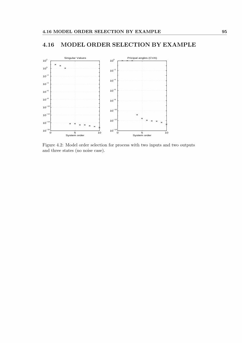
4.16 MODEL ORDER SELECTION BY EXAMPLE 95
4.16 MODEL ORDER SELECTION BY EXAMPLE
0 5 1010
−16
10−14
10−12
10−10
10−8
10−6
10−4
10−2
100
102
Singular Values
System order0 5 10
10−14
10−12
10−10
10−8
10−6
10−4
10−2
100
Pricipal angles (CVA)
System order
Figure 4.2: Model order selection for process with two inputs and two outputsand three states (no noise case).
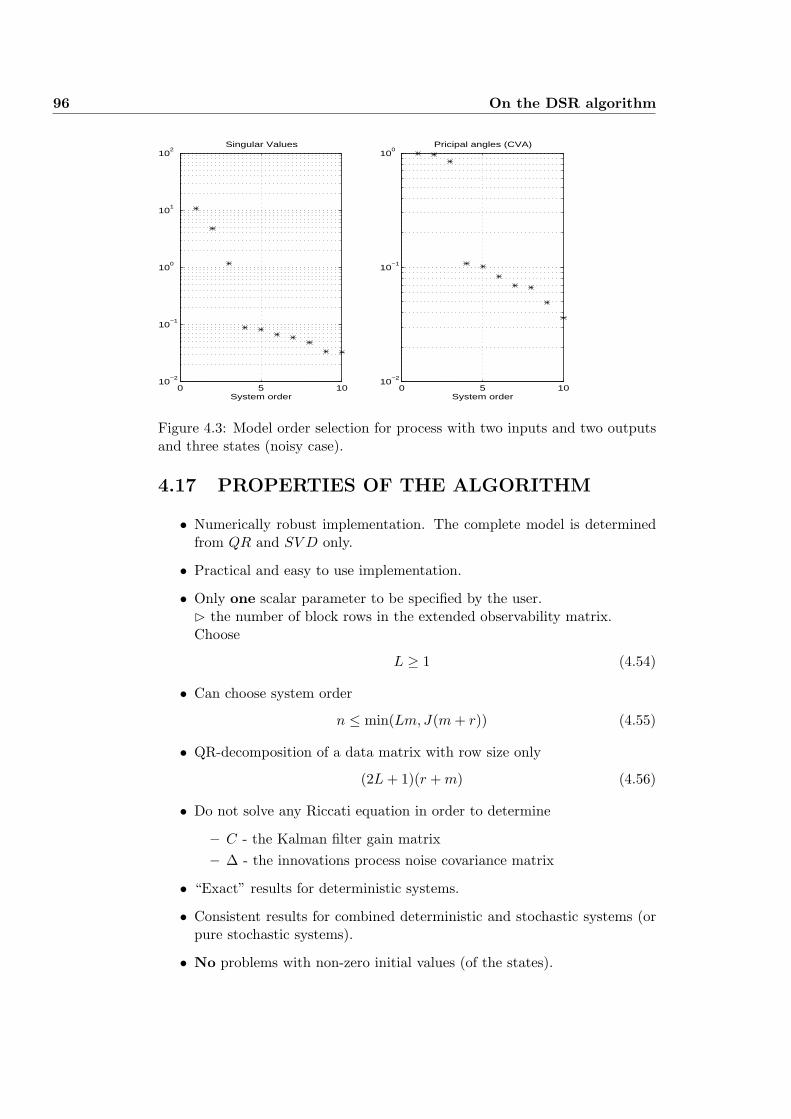
96 On the DSR algorithm
0 5 1010
−2
10−1
100
101
102
Singular Values
System order0 5 10
10−2
10−1
100
Pricipal angles (CVA)
System order
Figure 4.3: Model order selection for process with two inputs and two outputsand three states (noisy case).
4.17 PROPERTIES OF THE ALGORITHM
• Numerically robust implementation. The complete model is determinedfrom QR and SV D only.
• Practical and easy to use implementation.
• Only one scalar parameter to be specified by the user.¤ the number of block rows in the extended observability matrix.Choose
L ≥ 1 (4.54)
• Can choose system order
n ≤ min(Lm, J(m + r)) (4.55)
• QR-decomposition of a data matrix with row size only
(2L + 1)(r + m) (4.56)
• Do not solve any Riccati equation in order to determine
– C - the Kalman filter gain matrix– ∆ - the innovations process noise covariance matrix
• “Exact” results for deterministic systems.
• Consistent results for combined deterministic and stochastic systems (orpure stochastic systems).
• No problems with non-zero initial values (of the states).

4.18 COMPARISON WITH CLASSICAL APPROACHES 97
4.18 COMPARISON WITH CLASSICAL APPROACHES
1. Parameterizations:
• Classical PE approaches need a certain user-specified model param-eterization, so-called canonical forms.There has been an extensive amount of research to determine canon-ical forms.Many problems with canonical forms (minimal parameterizations).Can lead to numerically ill-conditioned problems, meaning that theparameters in the canonical form model is extremely sensitive tosmall perturbations.
• DSR method need no parameterization.
2. Convergence:
• PE approaches is iterative. Many hard to deal with problems suchasproblems with lack of convergence; no convergence; slow conver-gence;local minima; numerical instability;
• DSR method is non-iterative, there are no problems with conver-gence and the method is numerically robust.
3. Speed:DSR method faster than classical PE approaches (because the methodis non-iterative).

98 On the DSR algorithm
4.19 INDUSTRIAL APPLICATIONS
A short description is given of applications of the DSR identification methodfor analysis and modeling of five different industrial data sets.
1. Thermo Mechanical Pulping (TMP) refiner. Models successfullyidentified between almost all input and output variables in the process.
2. Paper machine. Dynamic model with 2 input and 2 output variablesidentified.
3. Plate column scrubber. 4 input and 5 output variables basic for mod-eling. (student project)
4. Raw oil distillation column. 4 input and 3 output variables are usedfor identifying a dynamic modeling.
5. Rotary oven. 4 input and 2 output variables are used for identifying adynamic model.
4.20 SOFTWARE 99
4.20 SOFTWARE
• DSR Toolbox for MATLAB. Fantoft Prosess A.S, P.O. Box 306, 1301Sandvika, Norway.
• DSR Windows 3.x, 95 or NT program. Fantoft Prosess A.S, P.O. Box306, 1301 Sandvika, Norway.
• Deterministic and Stochastic system identification and Realization (DSR).
How to use matlab script
Known process input and output data
uk ∀ k = 1, 2, ..., Nyk ∀ k = 1, 2, ..., N
}known
Organize into data matrices
Known data matrix of output variables︷ ︸︸ ︷
Y =
yT0
yT1
...yT
N−1
∈ RN×m (4.57)
Known data matrix of input variables︷ ︸︸ ︷
U =
uT0
uT1
...uT
N−1
∈ RN×r (4.58)
• Computing the dynamic model
[A,B,D,E,C,F ,x0
]= DSR(Y, U, L) (4.59)
• One scalar parameter L.
• Choose system order n ≤ min(Lm, J(m + r)).
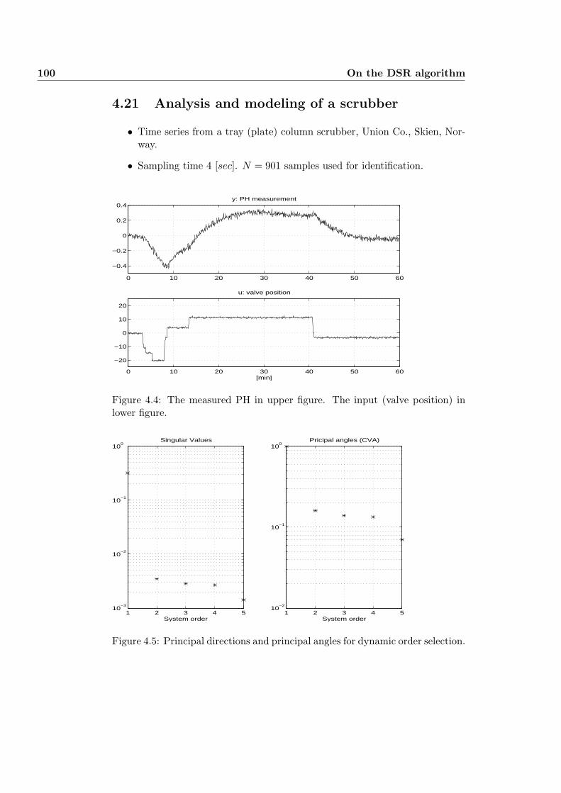
100 On the DSR algorithm
4.21 Analysis and modeling of a scrubber
• Time series from a tray (plate) column scrubber, Union Co., Skien, Nor-way.
• Sampling time 4 [sec]. N = 901 samples used for identification.
0 10 20 30 40 50 60
−0.4
−0.2
0
0.2
0.4y: PH measurement
0 10 20 30 40 50 60
−20
−10
0
10
20
[min]
u: valve position
Figure 4.4: The measured PH in upper figure. The input (valve position) inlower figure.
1 2 3 4 510
−3
10−2
10−1
100
Singular Values
System order1 2 3 4 5
10−2
10−1
100
Pricipal angles (CVA)
System order
Figure 4.5: Principal directions and principal angles for dynamic order selection.
4.22 MONTE CARLO SIMULATION OF MIMO SYSTEM 101
4.22 MONTE CARLO SIMULATION OF MIMOSYSTEM
System data:
Number of inputs: r = 2Number of outputs: m = 2Number of states: n = 3
Input experiment signal:
ut =[
sin( t14) + sin( t
7) + sin( t3)
(sin( t25) + sin( t
10) + sin( t5) + sin(t))0.2
] }Case 1: results in Figure 4.6
ut =[
(sin( t14) + sin( t
7) + sin( t3))0.05
(sin( t25) + sin( t
10) + sin( t5) + sin(t))0.1
] }Case 2: results in Figure 4.7
Noise covariance matrices:
E(wk) = 0, E(wkwTk ) =
[2 00 2
](4.60)
E(vk) = 0, E(vkvTk ) =
[1 00 1
]
Simulation parameters:
Number of samples: N = 5000Number of experiments: M = 100
Algorithms and parameters used:
DSR, L = 2CVA, Larimore (1990), I = 3ROBUST, Van Overschee (1995), I = 3
• For purely exiting input signals, choose DSR parameter L small.
• L is the horizon used to predict the number of states.
• For choice L = 2, must choose n ≤ Lm = 4.
• CVA and ROBUST: The smallest parameter is I = 3 in order to identifya 3rd order model.
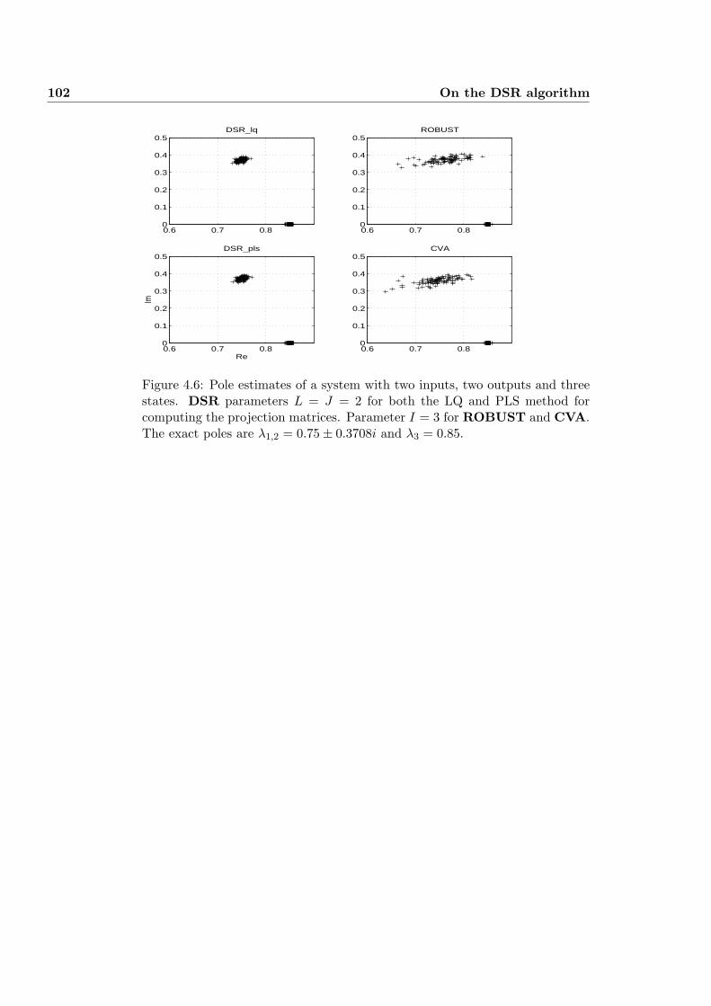
102 On the DSR algorithm
0.6 0.7 0.80
0.1
0.2
0.3
0.4
0.5DSR_lq
0.6 0.7 0.80
0.1
0.2
0.3
0.4
0.5ROBUST
0.6 0.7 0.80
0.1
0.2
0.3
0.4
0.5DSR_pls
Re
Im
0.6 0.7 0.80
0.1
0.2
0.3
0.4
0.5CVA
Figure 4.6: Pole estimates of a system with two inputs, two outputs and threestates. DSR parameters L = J = 2 for both the LQ and PLS method forcomputing the projection matrices. Parameter I = 3 for ROBUST and CVA.The exact poles are λ1,2 = 0.75± 0.3708i and λ3 = 0.85.
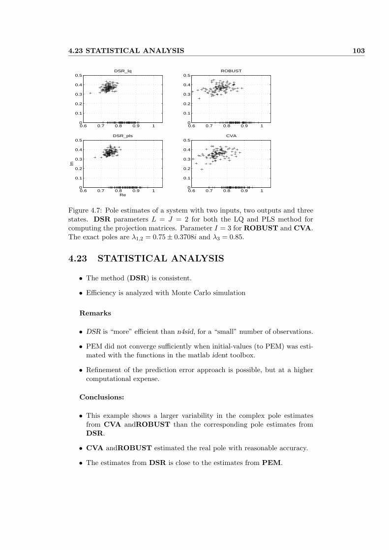
4.23 STATISTICAL ANALYSIS 103
0.6 0.7 0.8 0.9 10
0.1
0.2
0.3
0.4
0.5DSR_lq
0.6 0.7 0.8 0.9 10
0.1
0.2
0.3
0.4
0.5ROBUST
0.6 0.7 0.8 0.9 10
0.1
0.2
0.3
0.4
0.5DSR_pls
Re
Im
0.6 0.7 0.8 0.9 10
0.1
0.2
0.3
0.4
0.5CVA
Figure 4.7: Pole estimates of a system with two inputs, two outputs and threestates. DSR parameters L = J = 2 for both the LQ and PLS method forcomputing the projection matrices. Parameter I = 3 for ROBUST and CVA.The exact poles are λ1,2 = 0.75± 0.3708i and λ3 = 0.85.
4.23 STATISTICAL ANALYSIS
• The method (DSR) is consistent.
• Efficiency is analyzed with Monte Carlo simulation
Remarks
• DSR is “more” efficient than n4sid, for a “small” number of observations.
• PEM did not converge sufficiently when initial-values (to PEM) was esti-mated with the functions in the matlab ident toolbox.
• Refinement of the prediction error approach is possible, but at a highercomputational expense.
Conclusions:
• This example shows a larger variability in the complex pole estimatesfrom CVA andROBUST than the corresponding pole estimates fromDSR.
• CVA andROBUST estimated the real pole with reasonable accuracy.
• The estimates from DSR is close to the estimates from PEM.
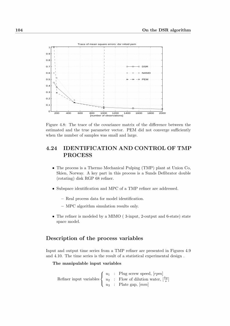
104 On the DSR algorithm
200 400 600 800 1000 1200 1400 1600 1800 20000
0.1
0.2
0.3
0.4
0.5
0.6
0.7
0.8
0.9
1
[number of observations]
Trace of mean square errors: dsr n4sid pem
DSR
N4SID
PEM
Figure 4.8: The trace of the covariance matrix of the difference between theestimated and the true parameter vector. PEM did not converge sufficientlywhen the number of samples was small and large.
4.24 IDENTIFICATION AND CONTROL OF TMPPROCESS
• The process is a Thermo Mechanical Pulping (TMP) plant at Union Co,Skien, Norway. A key part in this process is a Sunds Defibrator double(rotating) disk RGP 68 refiner.
• Subspace identification and MPC of a TMP refiner are addressed.
– Real process data for model identification.
– MPC algorithm simulation results only.
• The refiner is modeled by a MIMO ( 3-input, 2-output and 6-state) statespace model.
Description of the process variables
Input and output time series from a TMP refiner are presented in Figures 4.9and 4.10. The time series is the result of a statistical experimental design .
The manipulable input variables
Refiner input variables
u1 : Plug screw speed, [rpm]u2 : Flow of dilution water, [kg
s ]u3 : Plate gap, [mm]
4.24 IDENTIFICATION AND CONTROL OF TMP PROCESS 105
The following vector of input variables is defined
uk =
u1
u2
u3
k
∈ R3. (4.61)
The output variablesThe process outputs used for identification is defined as follows
Refiner output variables{
y1 : Refiner specific energy, [ MWh1000kg ]
y2 : Refiner consistency, [%]
The following vector of process output variables is defined
yk =[
y1
y2
]
k
∈ R2. (4.62)
106 On the DSR algorithm
Subspace identification
• Input and output time series from a TMP refiner are presented in Figures4.9 and 4.10. The time series is the result of a statistical experimentaldesign .
• The problem is to identify the SSM matrices (A,B, C,D, E, F ) (up towithin a similarity transformation), including the system order (n), di-rectly from known system input and output data vectors (or time series).
• The SSM is assumed to be on innovations form (Kalman filter).
The known process input and output data vectors from the TMP process canbe defined as follows
uk ∀ k = 1, . . . , Nyk ∀ k = 1, . . . , N
}Known data
For the TMP refiner example we have used:
N = 1500 [samples] for model identification860 [samples] for model validation
• Trends should preferably be removed from the data and the time seriesshould be adjusted for time delays. Data preprocessing is not necessarybut it often increase the accuracy of the estimated model.
The following constant trends (working points) are removed from the refinerinput and output data.
u0 =
52.37.0
0.58
, y0 =
[1.5934.3
](4.63)
4.24 IDENTIFICATION AND CONTROL OF TMP PROCESS 107
Organize the process output and input data vectors yk and uk as follows
Known data matrix of output variables︷ ︸︸ ︷
Y =
yT1
yT2
...yT
N
∈ RN×m (4.64)
Known data matrix of input variables︷ ︸︸ ︷
U =
uT1
uT2
...uT
N
∈ RN×r (4.65)
The problem of identifying a complete (usually) dynamic model for the processcan be illustrated by the following function (similar to a matlab function).
[A, B, C, D, E, F
]= DSR(Y, U,L) (4.66)
where the sixfold matrices (A, B,C, D,E, F ) are the state space model matrices.
• The algorithm name DSR stands for Deterministic and Stochastic modelRealization and identification.
• L is a positive integer parameter which should be specified by the user.
• The parameter L defines an upper limit for the unknown system order n.n ≤ Lm.
• The user must chose the system order by inspection of a plot with SingularValues (SV) or Principal Angles (PA). The system order n is identified asthe number of “non-zero” SV’s or “non-zero” PA’s.
• Note that the Kalman filter gain is given by K = CF−1 and that thecovariance matrix of the noise innovation process is given by E(vkv
Tk ) =
FF T .
• L = 3 and n = 6 where chosen in this example.
108 On the DSR algorithm
Model predictive control of TMP refiner
The following weighting matrices are used in the control objective.
Qi =[
100 00 100
], Ri =
0.5 0 00 0.1 00 0 100
, Pi = 0r, ∀ i = 1, · · · , L.(4.67)
The following horizons are used
Horizons in MPC algorithm{
L = 6, the prediction horizonJ = 6, the identification horizon
The following constraints are specified
umink =
50.06.00.5
, umax
k =
54.08.00.7
∀ k > 0 (4.68)
∆umink =
−0.5−0.15−0.05
, ∆umax
k =
0.50.150.05
∀ k > 0 (4.69)
ymink =
[1.533
], ymax
k =[
1.740
]∀ k > 0 (4.70)
Simulation results are illustrated in Figures 4.11 and 4.12.
4.25 References 109
4.25 References
Di Ruscio, D. (1997). A method for identification of combined deterministicstochastic systems. In: Applications of Computer Aided Time Series Mod-eling, Lecture Notes in Statistics 119, Eds. M. Aoki and A. M. Havenner,Springer Verlag, ISBN 0-387-94751-5.
Di Ruscio, D. and A. Holmberg (1996). Subspace identification for dynamicprocess analysis and modeling. Control Systems 96, Halifax, Nova Scotia,May 1996.
Golub, G. H. and C. F. Van Loan (1983). Matrix Computations. North OxfordAcademic Publishers Ltd.
Larimore, W. E. (1983). System identification, reduced order filtering andmodeling via canonical variate analysis. Proc. of the American ControlConference, San Francisco, USA, pp. 445-451.
Larimore, W. E. (1990). Canonical Variate Analysis in Identification, Filteringand Adaptive Control. Proc. of the 29th Conference on Decision andControl, Honolulu, Hawaii, December 1990, pp. 596-604.
Ljung, L. (1991). System Identification Toolbox. The Mathworks, Inc.
Faurre, P. L. (1976). Stochastic realization algorithms. In: System Identifica-tion: Advances and Case Studies, (eds. R. K. Mehra and D. G. Lainiotis),Academic Press.
Kung, S. Y. (1978). A new identification and Model Reduction Algorithm viaSingular Value Decomposition. Conf. on Circuits, Systems and Comput-ers, Pacific Grove, CA, November 1978, pp. 705-714.
Moore, B. C. (1981). Principal Component Analysis in Linear Systems: Con-trollability, Observability, and Model Reduction. IEEE Trans. on Auto-matic Control, Vol. AC-26, pp. 17-31.
Van Overschee, P. and B. De Moor (1994). N4SID: Subspace Algorithms forthe Identification of Combined Deterministic Stochastic Systems. Auto-matica, vol. 30, No. 1, pp.75-94.
Van Overschee, P. (1995). Subspace Identification: theory-implementation-application. PhD thesis, Katholieke Universiteit Leuven, Belgium.
Van Overschee, P. and B. De Moor (1995). A Unifying Theorem for ThreeSubspace System Identification Algorithms. Automatica, vol. 31, No. 12,pp. 1853-1864.
Verhagen, M. (1994). Identification of the deterministic part of MIMO statespace models given on innovations form from input output data. Auto-matica, vol. 30, No. 1, pp. 61-74.
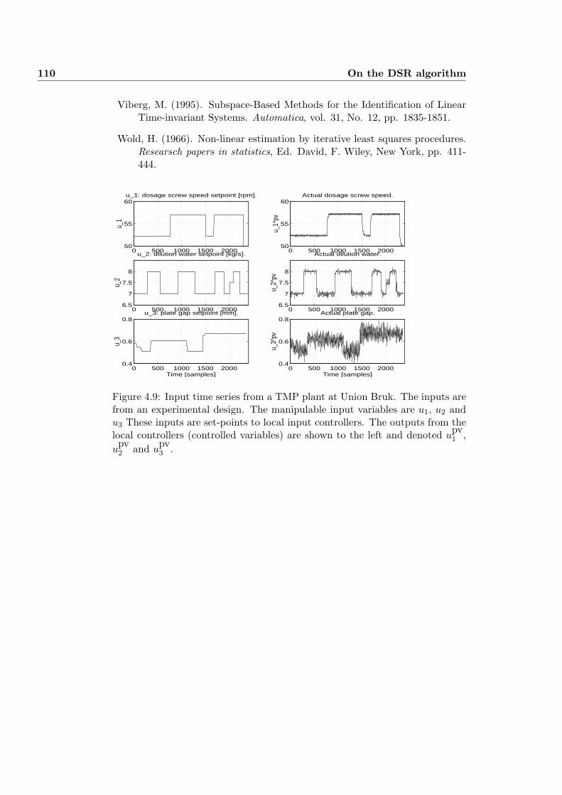
110 On the DSR algorithm
Viberg, M. (1995). Subspace-Based Methods for the Identification of LinearTime-invariant Systems. Automatica, vol. 31, No. 12, pp. 1835-1851.
Wold, H. (1966). Non-linear estimation by iterative least squares procedures.Researsch papers in statistics, Ed. David, F. Wiley, New York, pp. 411-444.
0 500 1000 1500 200050
55
60
u_1
u_1: dosage screw speed setpoint [rpm].
0 500 1000 1500 200050
55
60
u_1^
pv
Actual dosage screw speed.
0 500 1000 1500 20006.5
7
7.5
8
u_2
u_2: dilution water setpoint [kg/s].
0 500 1000 1500 20006.5
7
7.5
8u_
2^pv
Actual dilution water.
0 500 1000 1500 20000.4
0.6
0.8
Time [samples]
u_3
u_3: plate gap setpoint [mm].
0 500 1000 1500 20000.4
0.6
0.8
Time [samples]
u_3^
pv
Actual plate gap.
Figure 4.9: Input time series from a TMP plant at Union Bruk. The inputs arefrom an experimental design. The manipulable input variables are u1, u2 andu3 These inputs are set-points to local input controllers. The outputs from thelocal controllers (controlled variables) are shown to the left and denoted u
pv1 ,
upv2 and u
pv3 .
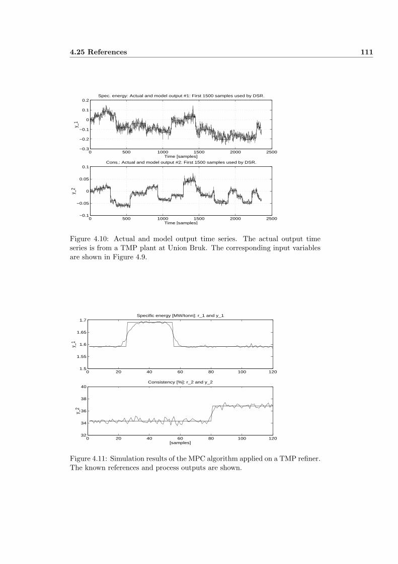
4.25 References 111
0 500 1000 1500 2000 2500−0.3
−0.2
−0.1
0
0.1
0.2
Time [samples]
y_1
Spec. energy: Actual and model output #1: First 1500 samples used by DSR.
0 500 1000 1500 2000 2500−0.1
−0.05
0
0.05
0.1
Time [samples]
y_2
Cons.: Actual and model output #2: First 1500 samples used by DSR.
Figure 4.10: Actual and model output time series. The actual output timeseries is from a TMP plant at Union Bruk. The corresponding input variablesare shown in Figure 4.9.
0 20 40 60 80 100 1201.5
1.55
1.6
1.65
1.7Specific energy [MW/tonn]: r_1 and y_1
y_1
0 20 40 60 80 100 12032
34
36
38
40Consistency [%]: r_2 and y_2
y_2
[samples]
Figure 4.11: Simulation results of the MPC algorithm applied on a TMP refiner.The known references and process outputs are shown.
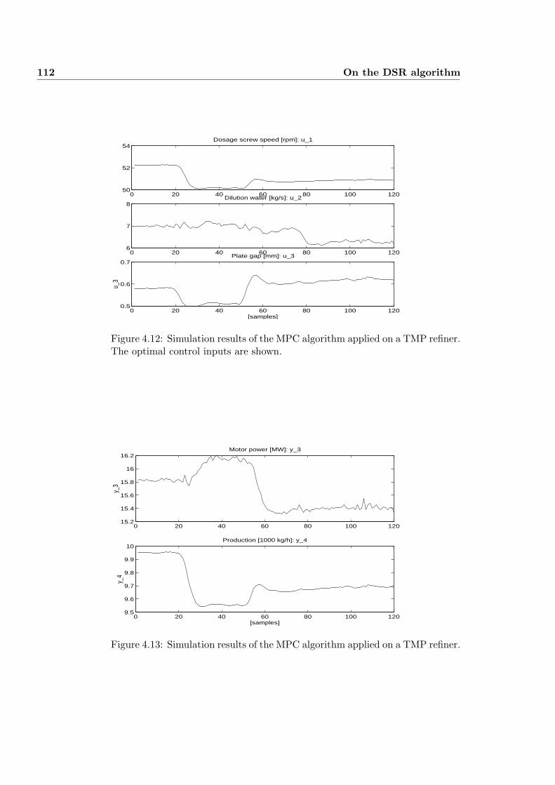
112 On the DSR algorithm
0 20 40 60 80 100 12050
52
54Dosage screw speed [rpm]: u_1
0 20 40 60 80 100 1206
7
8Dilution water [kg/s]: u_2
0 20 40 60 80 100 1200.5
0.6
0.7Plate gap [mm]: u_3
u_3
[samples]
Figure 4.12: Simulation results of the MPC algorithm applied on a TMP refiner.The optimal control inputs are shown.
0 20 40 60 80 100 12015.2
15.4
15.6
15.8
16
16.2Motor power [MW]: y_3
y_3
0 20 40 60 80 100 1209.5
9.6
9.7
9.8
9.9
10Production [1000 kg/h]: y_4
y_4
[samples]
Figure 4.13: Simulation results of the MPC algorithm applied on a TMP refiner.
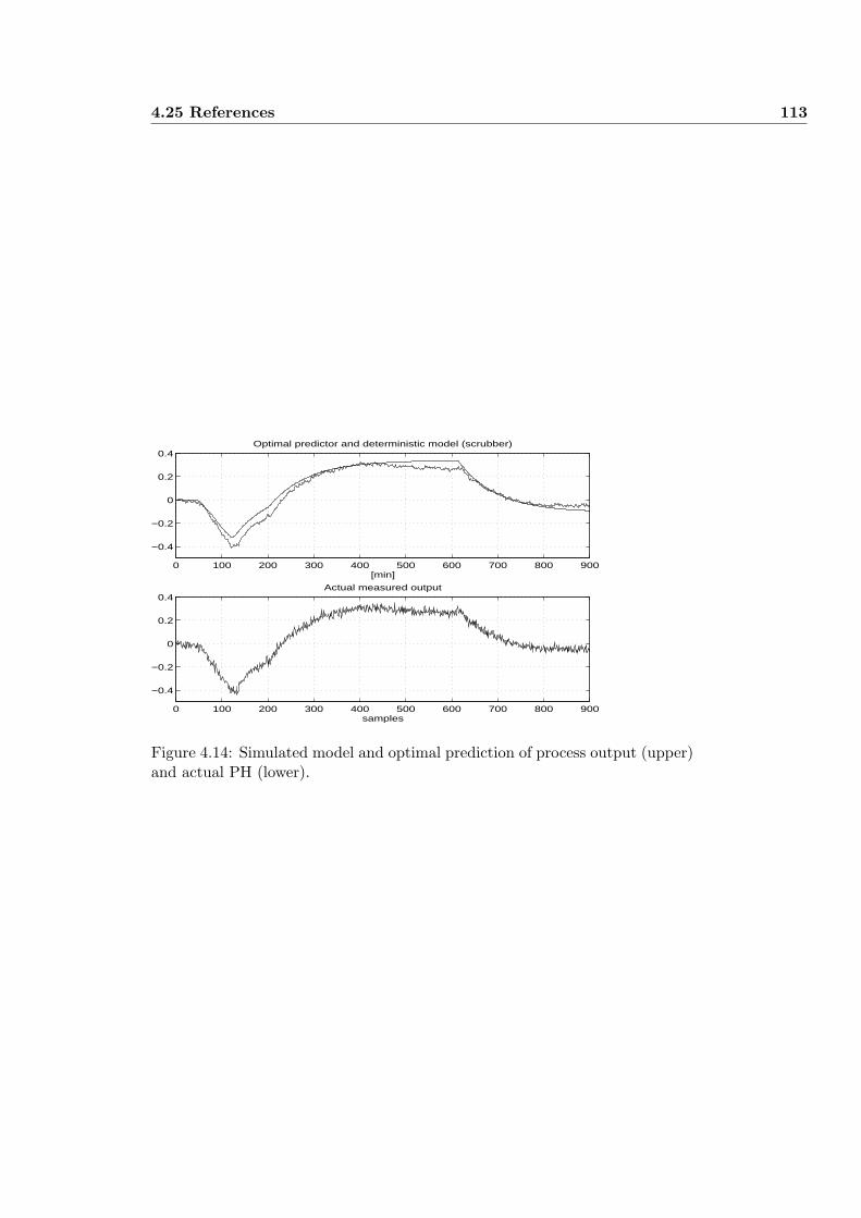
4.25 References 113
0 100 200 300 400 500 600 700 800 900
−0.4
−0.2
0
0.2
0.4Optimal predictor and deterministic model (scrubber)
[min]
0 100 200 300 400 500 600 700 800 900
−0.4
−0.2
0
0.2
0.4Actual measured output
samples
Figure 4.14: Simulated model and optimal prediction of process output (upper)and actual PH (lower).

114 On the DSR algorithm
Chapter 5
Subspace Identification forDynamic Process Analysis andModeling
Abstract
A recently developed subspace identification method for robust data analysisand modeling of dynamic and static systems from known observations will bepresented. The method is used in order to analyze and modeling time seriesfrom an Thermo Mechanical Pulping refiner line at Norske Skog, Norway.
Keywords: Subspace identification; time series; TMP refiners; power; specificenergy; system identification; practical results.
5.1 Introduction
The subspace method discussed in this work, [3] - [6], has a number of ad-vantages compared to the traditional prediction error approaches for systemidentification. The method is practical and easy to use, it is non-iterative, al-ways convergent and completely data driven. See also [8] and the survey paper[9].
The method detects system dynamics (system order) and it can be viewedas a generalization of traditional multivariate data analysis and modeling meth-ods such as Principal Component Analysis (PCA) and Regression (PCR) andPartial Least Squares (PLS). These last methods all deals with analyzing andmodeling of static relationship between variables and are well known methodsin e.g., chemometrics and econometrics. However, these methods are insuffi-cient in order to modeling data from dynamical systems, i.e., systems wherethe direction of time is important.
This implies that PCA, PCR and PLS deals with a special case analysis and
116 Subspace Identification for Dynamic Process Analysis and Modeling
modeling problem of the problem which is solved by the subspace methods.
The first step in the subspace method is a data compression step. The pos-sibly large number of observations (data) are compressed to a much smaller ma-trix by a standard lower Left Q-orthogonal (LQ) decomposition. This smallerlower triangular matrix contains the information of the system (process and sen-sors) which generated the data. The system dynamics as well as the completemodel for the system is extracted from this smaller matrix. A short descriptionof how to use the method will be given in this paper.
Note that the method works for systems where the outputs are driven byboth known input variables and unknown process disturbance variables. Theunknown variables may be high frequency or colored noise variables. Themethod is believed to be a valuable tool for analyzing and modeling of data fromindustrial processes, in particular dynamic processes. The subspace method isused on some important processes in the pulp and paper industry in Norway,e.g. a plate column scrubber; a paper machine; the Thermo Mechanical Pulping(TMP) process.
The process variables measured on a two stage TMP refiner line at NorskeSkog, Skogn, Norway are analyzed and modeled by the method. In particular,a state space model for the refiner motor power is constructed from observeddata (time series). This results will be presented in the paper. The model forthe 1st stage refiner has three input variables, i.e., plug screw speed, dilutionwater and plate gap. The power model will be presented in this paper.
The rest of this paper is organized as follows. Some preliminary system andproblem definitions are stated in Section 5.2. A description of the subspacemethod is presented in Section 5.3. An application of the subspace method[6] is presented in Section 5.4. The actual process is a two-stage TMP refinerline at Norske Skog, Skogn, Norway. A state space model for the TMP refinermotor power is identified. Some conclusions follows in Section 5.5.
5.2 Preliminary definitions
5.2.1 System definition
Assume that the underlying system can be described by a discrete-time, timeinvariant, linear state space model (SSM) of the form
xk+1 = Axk + Buk + Cek (5.1)yk = Dxk + Euk + ek (5.2)
where the integer k ≥ 0 is discrete-time, x ∈ Rn is the state vector with initialvalue x0, y ∈ Rm is the system output, u ∈ Rr is the system input, e ∈ Rm
is an unknown innovations process of white noise, assumed to be covariancestationary, with zero mean and covariance matrix E(eke
Tk ) = ∆. The constant
matrices in the SSM are of appropriate dimensions. A is the state transition
5.3 Description of the method 117
matrix, B is the external input matrix, C is the Kalman gain matrix, D isthe output matrix and E is the direct control input to output (feed-through)matrix. We will assume that (D, A) is an observable pair.
The innovations model, Equations (5.1) and (5.2), is discussed in e.g. [7],[1].
5.2.2 Problem definition
The problem investigated in this paper is to identify a state space model, in-cluding the system order (n), for both the deterministic part and the stochasticpart of the system, i.e., the quadruple matrices (A,B, D,E) and the double ma-trices (C, ∆), respectively, directly from known system input and output datavectors (or time series) defined as
uk ∀ k = 0, . . . , N − 1yk ∀ k = 0, . . . , N − 1
}Known data
Note that the variables can be linearly dependent as well as independent. Incontinuous time systems the matrix E in Equation (5.2) is usually zero. Thisis not the case in discrete time systems due to sampling. However, E can beforced to be zero by including a structure constraint in the algorithm, [6].
5.3 Description of the method
Given sequences with process input and output raw data. The first step ina data modeling procedure is usually to analyze the data for trends and timedelays. Trends should preferably be removed from the data and the time seriesshould be adjusted for time delays. The trend of a time series can often beestimated as the sample mean which represents some working point. Data pre-processing is not necessary but it usually increase the accuracy of the estimatedmodel.
The simplicity of the subspace method [6] will be illustrated in the following.Assume that the data is adjusted for trends and time delays. Organize theprocess output and input data vectors yk and uk as follows
Known data matrix of output variables︷ ︸︸ ︷
Y =
yT0
yT1
...yT
N−1
∈ <N×m (5.3)
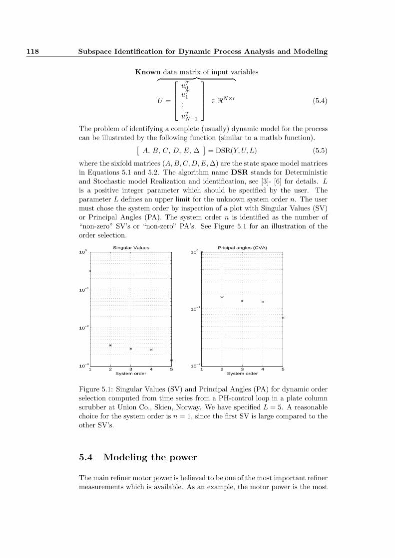
118 Subspace Identification for Dynamic Process Analysis and Modeling
Known data matrix of input variables︷ ︸︸ ︷
U =
uT0
uT1
...uT
N−1
∈ <N×r (5.4)
The problem of identifying a complete (usually) dynamic model for the processcan be illustrated by the following function (similar to a matlab function).
[A, B, C, D, E, ∆
]= DSR(Y, U, L) (5.5)
where the sixfold matrices (A,B, C,D, E,∆) are the state space model matricesin Equations 5.1 and 5.2. The algorithm name DSR stands for Deterministicand Stochastic model Realization and identification, see [3]- [6] for details. Lis a positive integer parameter which should be specified by the user. Theparameter L defines an upper limit for the unknown system order n. The usermust chose the system order by inspection of a plot with Singular Values (SV)or Principal Angles (PA). The system order n is identified as the number of“non-zero” SV’s or “non-zero” PA’s. See Figure 5.1 for an illustration of theorder selection.
1 2 3 4 510
−3
10−2
10−1
100
Singular Values
System order1 2 3 4 5
10−2
10−1
100
Pricipal angles (CVA)
System order
Figure 5.1: Singular Values (SV) and Principal Angles (PA) for dynamic orderselection computed from time series from a PH-control loop in a plate columnscrubber at Union Co., Skien, Norway. We have specified L = 5. A reasonablechoice for the system order is n = 1, since the first SV is large compared to theother SV’s.
5.4 Modeling the power
The main refiner motor power is believed to be one of the most important refinermeasurements which is available. As an example, the motor power is the most
5.4 Modeling the power 119
important variable in order to estimate the consistency, the specific energy andthe steam which is generated in the refiner. The motor power is an outputfrom the refining process. The power should be modeled as a function of therefiner input variables. A combined mechanistic and empirical power model isdiscussed in [2]. For a CD refiner we have the following input variables; dosagescrew speed ns; plate gap for the plane zone s1; plate gap for the conical zones2; flow rate of dilution water to the refiner inlet or plane zone qw1 and to theconical zone qw2. The power model can be formulated as
y = y(ns, qw1, qw2, s1, s2) (5.6)
where y is the refiner motor power. Another procedure is to identify a model forthe refiner motor power, directly from measured input and output data. Thisapproach will be discussed in the rest of this section.
5.4.1 Refiner variables and model
The manipulable input variables are defined as follows
u ∈ <3 :=
u1 Plug screw speed, [rpm]u2 Total flow of dilution water, [kg
s ]u3 Plate gap, conical zone, [mm]
(5.7)
The linearized power model is assumed to be on innovations form, Equation5.1 and 5.2. The innovations model can be written as an optimal predictor forthe power output yt given all past process inputs and outputs. The optimalprediction of the power can be computed from
xt+1 = Axt + But + C(yt −Dxt −Eut) (5.8)yt = Dxt + Eut (5.9)
where yt is the optimal prediction of the present output yt given all past outputs(..., yt−2, yt−1) and the present and all past inputs (..., ut−1, ut). The problemis to find the model matrices (A,B, C, D, E) and the covariance matrix of theinnovations noise process, ∆ = cov(ete
Tt ).
We will also mention that the combined deterministic and stochastic model,Equations 5.1 and 5.2, can be separated into two parts. One deterministic part(with output yd
t ) which is driven by the known process input variables ut andone stochastic part (with output ys
t ) driven by the unknown innovations noiseprocess et. The actual output is then yt = yd
t + yst . See e.g., [2] p. 36.
We will in this work focusing on modeling the 1st stage refiner motor power.It is often not clear whether a process variable should be defined as an inputor output variable to a model. An example of this is the problem of modelingthe 2nd stage refiner. It is assumed that the 1st stage motor power yt containsinformation of the disturbances which affects the 2nd stage refiner. Hence, theinclusion of the output yt as an additional input to the power model for the2nd stage refiner is reasonable. We will not elaborate this further.
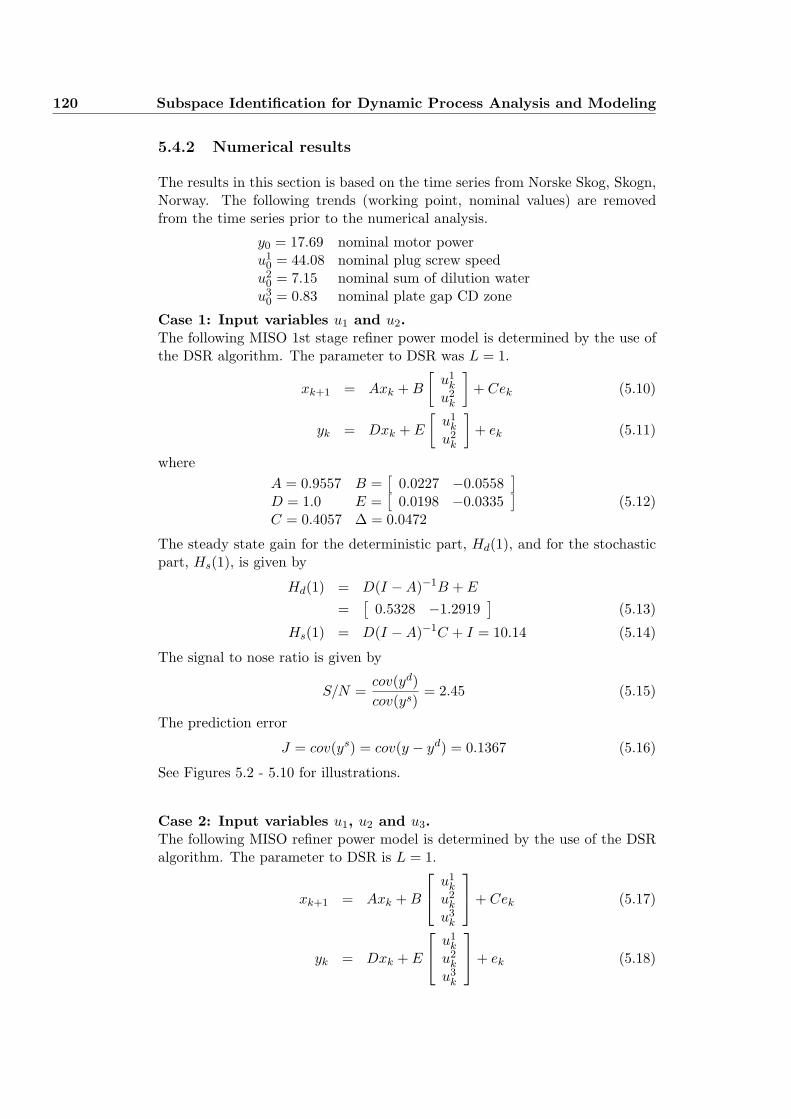
120 Subspace Identification for Dynamic Process Analysis and Modeling
5.4.2 Numerical results
The results in this section is based on the time series from Norske Skog, Skogn,Norway. The following trends (working point, nominal values) are removedfrom the time series prior to the numerical analysis.
y0 = 17.69 nominal motor poweru1
0 = 44.08 nominal plug screw speedu2
0 = 7.15 nominal sum of dilution wateru3
0 = 0.83 nominal plate gap CD zone
Case 1: Input variables u1 and u2.The following MISO 1st stage refiner power model is determined by the use ofthe DSR algorithm. The parameter to DSR was L = 1.
xk+1 = Axk + B
[u1
k
u2k
]+ Cek (5.10)
yk = Dxk + E
[u1
k
u2k
]+ ek (5.11)
whereA = 0.9557 B =
[0.0227 −0.0558
]D = 1.0 E =
[0.0198 −0.0335
]C = 0.4057 ∆ = 0.0472
(5.12)
The steady state gain for the deterministic part, Hd(1), and for the stochasticpart, Hs(1), is given by
Hd(1) = D(I −A)−1B + E
=[
0.5328 −1.2919]
(5.13)
Hs(1) = D(I −A)−1C + I = 10.14 (5.14)
The signal to nose ratio is given by
S/N =cov(yd)cov(ys)
= 2.45 (5.15)
The prediction error
J = cov(ys) = cov(y − yd) = 0.1367 (5.16)
See Figures 5.2 - 5.10 for illustrations.
Case 2: Input variables u1, u2 and u3.The following MISO refiner power model is determined by the use of the DSRalgorithm. The parameter to DSR is L = 1.
xk+1 = Axk + B
u1k
u2k
u3k
+ Cek (5.17)
yk = Dxk + E
u1k
u2k
u3k
+ ek (5.18)
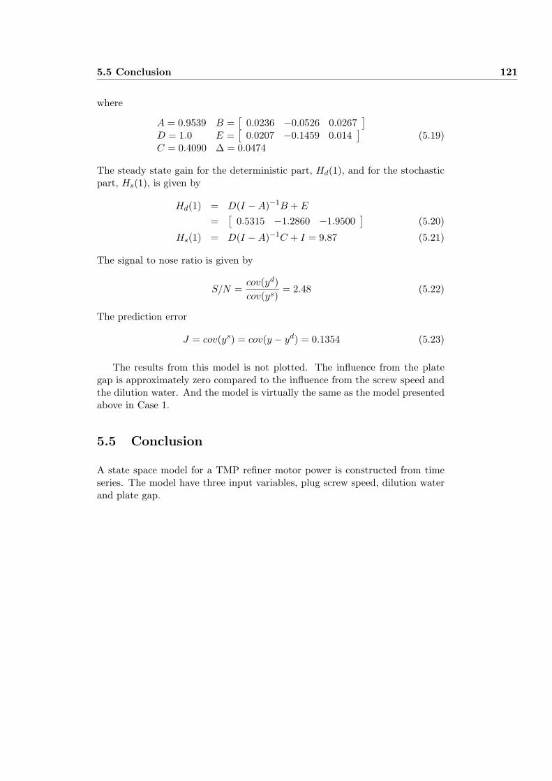
5.5 Conclusion 121
where
A = 0.9539 B =[
0.0236 −0.0526 0.0267]
D = 1.0 E =[
0.0207 −0.1459 0.014]
C = 0.4090 ∆ = 0.0474(5.19)
The steady state gain for the deterministic part, Hd(1), and for the stochasticpart, Hs(1), is given by
Hd(1) = D(I −A)−1B + E
=[
0.5315 −1.2860 −1.9500]
(5.20)
Hs(1) = D(I −A)−1C + I = 9.87 (5.21)
The signal to nose ratio is given by
S/N =cov(yd)cov(ys)
= 2.48 (5.22)
The prediction error
J = cov(ys) = cov(y − yd) = 0.1354 (5.23)
The results from this model is not plotted. The influence from the plategap is approximately zero compared to the influence from the screw speed andthe dilution water. And the model is virtually the same as the model presentedabove in Case 1.
5.5 Conclusion
A state space model for a TMP refiner motor power is constructed from timeseries. The model have three input variables, plug screw speed, dilution waterand plate gap.

122 Subspace Identification for Dynamic Process Analysis and Modeling
Bibliography
[1] M. Aoki, “State Space Modeling of Time Series,” Springer-Verlag, 1990.
[2] D. Di Ruscio, Topics in model based control with application to the thermomechanical pulping process, Dr. Ing. thesis. Report no. 93-46-W. Divisionof Engineering Cybernetics, NTH, N-7034 Trondheim, 1993.
[3] D. Di Ruscio, “A Method for identification of combined deterministic andstochastic system,” In Proceedings of the European Control Conference,ECC95, Roma, Italy, September 5-8, 1995.
[4] D. Di Ruscio, “Methods for the identification of state space models frominput and output measurements,” SYSID 94, The 10th IFAC Symposiumon System Identification, Copenhagen, July 4 - 6, 1994. Also in: Modeling,Identification and Control, Vol. 16, no. 3, 1995.
[5] D. Di Ruscio, “Identification and Realization of Combined Deterministicand Stochastic Systems,” To be included in: Lecture Notes in Time SeriesAnalysis, (edited by M. Aoki, UCLA,USA), 1996.
[6] “DSR: Algorithm for combined deterministic and stochastic system identi-fication and realization of state space models from observations,” Programcommercial available by Fantoft Process AS, Box 306, N-1301 Sandvika.
[7] P. L. Faurre, “Stochastic Realization Algorithms,” In: System Identifi-cation: Advances and Case Studies, (edited by R. K. Mehra and D. G.Lainiotis), Academic Press, 1976.
[8] W. E. Larimore, “Canonical Variate Analysis in Identification, Filteringand Adaptive Control,” Proc. of the 29th Conference on Decision and Con-trol, Honolulu, Hawaii, december 1990, pp. 596-604.
[9] M. Viberg, “Subspace-Based Methods for the Identification of Linear TimeInvariant Systems,” Automatica, vol. 31, No. 12, pp. 1835-1851.
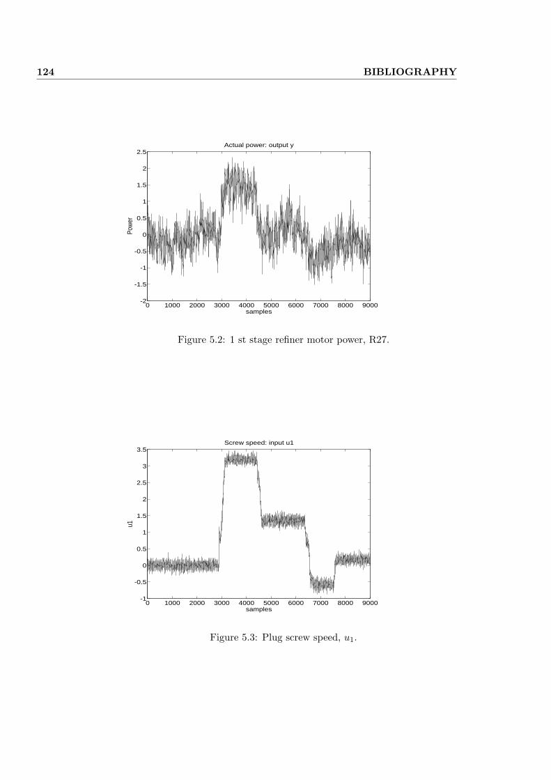
124 BIBLIOGRAPHY
0 1000 2000 3000 4000 5000 6000 7000 8000 9000-2
-1.5
-1
-0.5
0
0.5
1
1.5
2
2.5Actual power: output y
Pow
er
samples
Figure 5.2: 1 st stage refiner motor power, R27.
0 1000 2000 3000 4000 5000 6000 7000 8000 9000-1
-0.5
0
0.5
1
1.5
2
2.5
3
3.5Screw speed: input u1
u1
samples
Figure 5.3: Plug screw speed, u1.
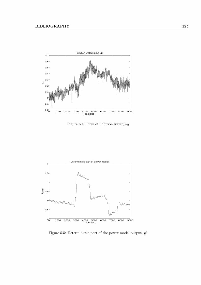
BIBLIOGRAPHY 125
0 1000 2000 3000 4000 5000 6000 7000 8000 9000-0.2
-0.1
0
0.1
0.2
0.3
0.4
0.5
0.6
0.7Dilution water: input u2
u2
samples
Figure 5.4: Flow of Dilution water, u2.
0 1000 2000 3000 4000 5000 6000 7000 8000 9000-1
-0.5
0
0.5
1
1.5
2Deterministic part of power model
Pow
er
samples
Figure 5.5: Deterministic part of the power model output, yd.
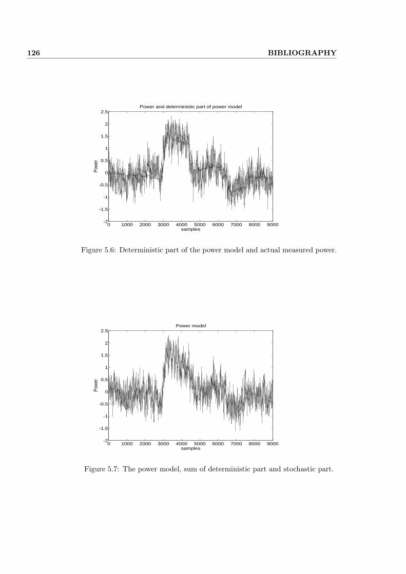
126 BIBLIOGRAPHY
0 1000 2000 3000 4000 5000 6000 7000 8000 9000-2
-1.5
-1
-0.5
0
0.5
1
1.5
2
2.5Power and deterministic part of power model
Pow
er
samples
Figure 5.6: Deterministic part of the power model and actual measured power.
0 1000 2000 3000 4000 5000 6000 7000 8000 9000-2
-1.5
-1
-0.5
0
0.5
1
1.5
2
2.5Power model
Pow
er
samples
Figure 5.7: The power model, sum of deterministic part and stochastic part.
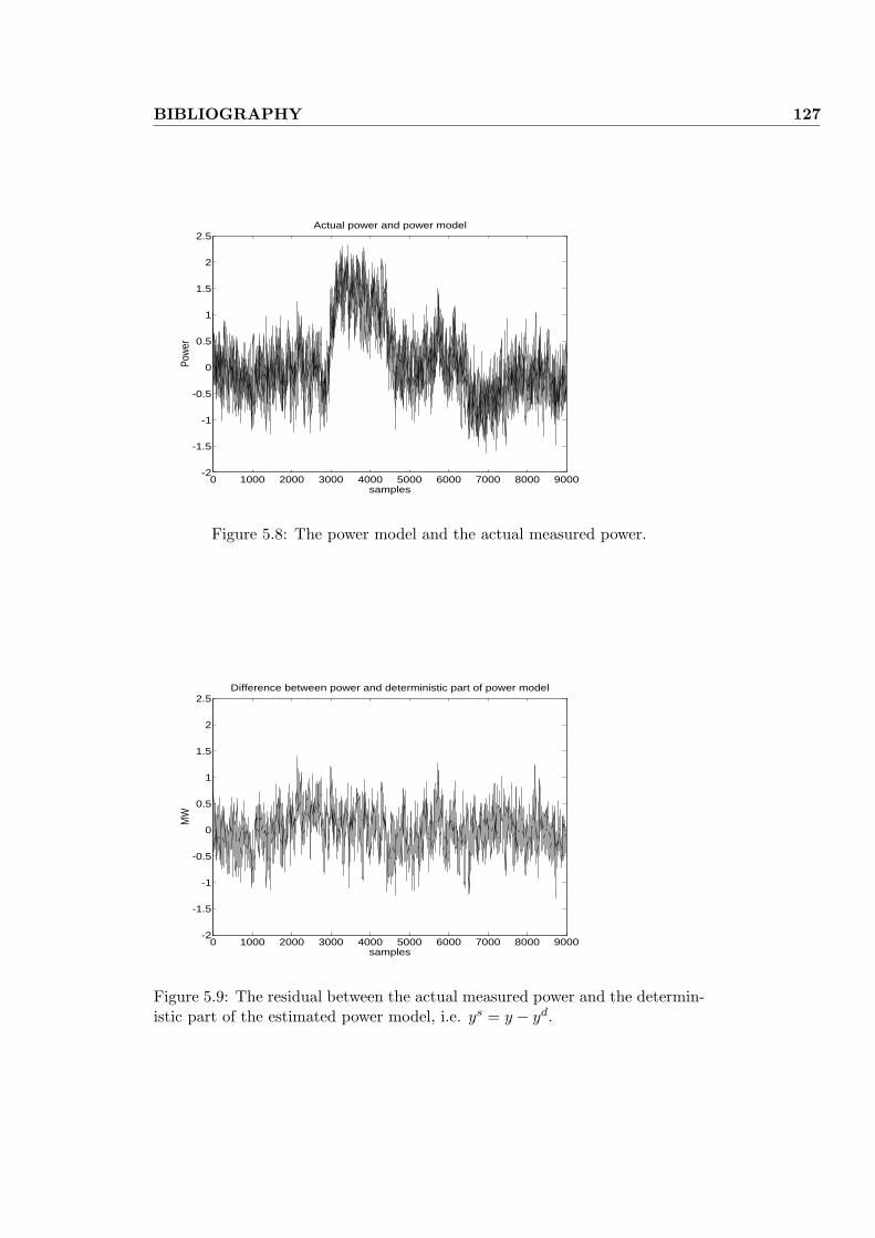
BIBLIOGRAPHY 127
0 1000 2000 3000 4000 5000 6000 7000 8000 9000-2
-1.5
-1
-0.5
0
0.5
1
1.5
2
2.5Actual power and power model
Pow
er
samples
Figure 5.8: The power model and the actual measured power.
0 1000 2000 3000 4000 5000 6000 7000 8000 9000-2
-1.5
-1
-0.5
0
0.5
1
1.5
2
2.5
samples
MW
Difference between power and deterministic part of power model
Figure 5.9: The residual between the actual measured power and the determin-istic part of the estimated power model, i.e. ys = y − yd.
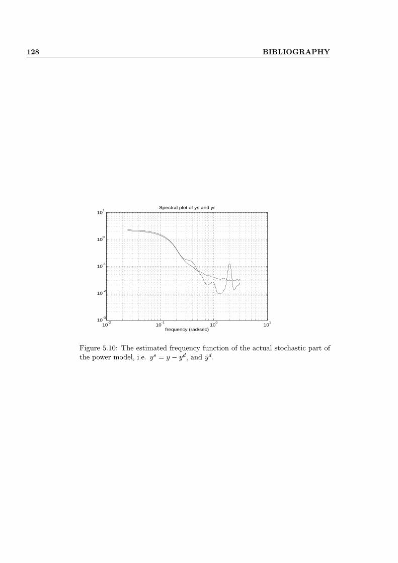
128 BIBLIOGRAPHY
10-2
10-1
100
101
10-3
10-2
10-1
100
101
frequency (rad/sec)
Spectral plot of ys and yr
Figure 5.10: The estimated frequency function of the actual stochastic part ofthe power model, i.e. ys = y − yd, and yd.
Chapter 6
Dynamic Subspace Modeling(DSR) and Static MultivariateAnalysis and Regression(PCA,PCR,PLS)
Abstract
It is shown that a solution to the multivariate analysis and regression problemis a special case of a recently developed subspace method for analysis and iden-tification of combined deterministic and stochastic dynamical systems. Thismethod detects system dynamics. A numerically stable solution to the multi-variate analysis and regression problem is also presented. Keywords: Systemidentification; subspace methods; dynamic systems; combined deterministic andstochastic systems; multivariate analysis and regression; PCR; PLS; data anal-ysis and modeling.
6.1 Introduction
The theory of multivariate analysis and regression is a research field in manydisciplines, e.g. in chemistry and economics. Econometrics and chemometricsare well established disciplines. A problem in many disciplines, including eco-nomics and chemistry, is to postulate relationships between variables. It is thepurpose of econometrics to postulate the relationship between economic vari-ables. In the same way one can state that a purpose of chemometrics is topostulate relationships between chemical variables. This problem is of greatimportance in general.
Solution procedures such as Partial Least Squares (PLS) and Principal Com-ponent regression (PCR) are effective tools for analysis and regression of pa-
130Dynamic Subspace Modeling (DSR) and Static Multivariate Analysis and
Regression (PCA,PCR,PLS)
rameters in systems which is static. I.e. these tools are effective to analyze andmodeling variables that are static related.
On the other side it can be very ineffective to use these methods to ana-lyze, modeling and identify (input output) relationships between variables in adynamical system.
One goal of statistical planning of system experiments is to produce datawhich is rich of system information. The system input variables which aremanipulable are perturbed in such a way that some invert-ability requirementof the manipulable variables is satisfied. However, it is important that all theparameters in the system is exited (in order to identify them). The systeminput and output variables are observed over the experimental period.
Usually all systems are dynamic in nature. In order to use PLS and PCRmethods, to analyze the system input and output behavior, one have to wait forall the transients to die out in order to e.g. identify the gain from the variableswhich are manipulated to the observed variables. All the observations in thetransient period are wasted. The result of this identification procedure usuallygives a wrong conclusion about the gain. The system output is in addition tothe manipulable variables driven by noise. It is known from the identificationtheory that the system gain can be identified before the transients in the systemhave died out. PLS and PCR methods can not detect dynamics and handledynamical systems in a proper way. For such systems, methods which candetect the dynamics, including the system order are prefered.
A so called subspace method for identification of combined deterministicand stochastic systems directly from the data is presented in Di Ruscio (1994),Di Ruscio (1994a) and Di Ruscio (1995). The starting point for this method isto allow a more general model structure for the system in which the standardstatic multivariate analysis and regression problem is a special case.
A fundamental property of this method is that the system dynamics (systemorder) are identified from the data. If the system order is identified to be zerothen a typical static regression problem results, in which PLS or PCR techniquescan be applied. The system order is not the same as the number of principalcomponents in PCR and number of factors (components) in PLS. The numberof principal components and PLS factors are measures of the effective rank of asequence of input (or output) variable observations. It is more or less the sameas what is called persistently exiting analysis of the input signal in classicalidentification theory.
Section 6.2 gives a system description of both the static and the dynamicmodeling problem and how the data is ordered into certain data matrices forwhich informations about the underlying system can be retrieved.
Section 6.4 gives a review of the solution to the more general dynamicsystem analysis and modeling problem. The first step is to compress the datadown to the square root of some covariance matrices. The next step is toidentify the system dynamics (system order). If the system order is detectedor specified to be zero then, the covariance matrices for the static problem are
6.2 System description and data organization 131
directly extracted. This method gives a numerically stable way of identifyingthe system order and the matrices in a so called combined deterministic andstochastic dynamic model.
The static analysis and regression modeling problem will be discussed inSection 6.5. In Lindgren, Geladi and Wold (1993) a covariance based PLSmethod is presented. The first step in this method is to compute the covariancematrices which is an ill-conditioned step. The next step is then to use a modifiedPLS method which works on the covariance matrices.
Another solution to this special static analysis and modeling problem will bepresented in this paper. This includes a numerically stable method to compressthe data down to the square root of the covariance matrices, without explicitlyforming the covariance matrices. In the next step, the standard PLS, SVD orPCR methods can be used.
6.2 System description and data organization
We will in this section give a system description. A system description is impor-tant because it is the fundament of the method to be presented. A poor systemdescription usually results in limitations of any method and algorithm. We willin Section 6.2.1 give a description of the more general combined deterministicand stochastic system. Section 6.2.1 gives a description of the less general staticsystem which is the fundament for the traditional analysis and regression toolsas PCA, PCR and PLS. The latter is a special case of the system descriptionin Section 6.2.2.
6.2.1 Combined deterministic and stochastic description
Assume that the underlying system can be described by a discrete-time, timeinvariant, linear state space model of the form
xk+1 = Axk + Buk + Cek (6.1)yk = Dxk + Euk + ek (6.2)
where k ≥ 0 is discrete-time, i.e. an integer, x ∈ <n is the state vector withinitial value x0, y ∈ <m is the system output, u ∈ <r is the system input, e ∈ <m
is an unknown innovations process of white noise, assumed to be covariancestationary, with zero mean and covariance matrix E(eke
Tk ) = ∆. A, B, C,
D and E are constant matrices of appropriate dimensions, where (D, A) is anobservable pair.
A solution to the identification problem of constructing a state space model,including the system order (n), for both the deterministic part and the stochas-tic part of the system i.e. the quadruple (A,B,D, E) and the double (C, ∆),respectively, directly from known input and output time series uk and yk.
132Dynamic Subspace Modeling (DSR) and Static Multivariate Analysis and
Regression (PCA,PCR,PLS)
Given the system output and input time series, yk∀k = 0, . . . , N − 1 anduk∀k = 0, . . . , N − 1, respectively. The state space model, Equations (6.1) and(6.2), can generally be written as
Yk+1 = AYk + BUk + CEk (6.3)
where
Yk =
yk yk+1 yk+2 · · · yk+K−1
yk+1 yk+2 yk+3 · · · yk+K...
......
. . ....
yk+L−1 yk+L yk+L+1 · · · yk+L+K−2
∈ <Lm×K (6.4)
Uk =
uk uk+1 uk+2 · · · uk+K−1
uk+1 uk+2 uk+3 · · · uk+K...
......
. . ....
uk+L−1 uk+L uk+L+1 · · · uk+L+K−2
uk+L uk+L+1 uk+L+2 · · · uk+L+K−1
∈ <(L+1)r×K(6.5)
Ek =
ek ek+1 ek+2 · · · ek+K−1
ek+1 ek+2 ek+3 · · · ek+K...
......
. . ....
ek+L−1 ek+L ek+L+1 · · · ek+L+K−2
ek+L ek+L+1 ek+L+2 · · · ek+L+K−1
∈ <(L+1)m×K(6.6)
The number of columns in Yk, Uk and Ek are K = N−L−k+1. Each column inthese matrices can be interpreted as extended output, input and noise vectors,respectively. K can be viewed as the number of samples in these extended timeseries. We also have that L < K < N . L is a user specified parameter whichis the number of block rows in the extended observability matrix which will bedetermined.
6.2.2 Purely static description
A model suitable for PLS and PCR problems can be written as the followinglinear steady state equation.
yTt = uT
t ET + eTt (6.7)
where yt ∈ <m is a vector of known output variables at observation number t.ut ∈ <r is a vector of known input variables and et ∈ <m is a vector of unknownwhite noise variables, assumed to be covariance stationary, with zero mean andcovariance matrix E(ete
Tt ) = ∆.
Assume a number of N observations, i.e. t = 1, ..., N . The N equationscan then be formed into the following matrix equation with notations which iscommon in multivariate regression theory.
Y = XB + E (6.8)
6.2 System description and data organization 133
where Y ∈ <N×m is a known matrix of observations. The vector yTt is also
called a vector of responses at observation number t. X ∈ <N×r is a knownmatrix of input variables. Each row in X (i.e. uT
t ) is also called a vectorof predictor variables at observation number t. The matrix B ∈ <r×m is thematrix of unknown parameters (also called regression coefficients).
Both data matrices Y and X can be corrupted with (measurements) noise.The principal components, detected as a first step in the PCR method, are thenumber of linearly independent columns in the data matrix X. This possiblyrank deficiency problem can e.g. be detected as the number of “non-zero”singular values which results from the Singular Value Decomposition (SVD) ofthe covariance matrix estimate 1
N XT X.
The (principal) components in the PLS method are computed by takingadvantage of both Y and X variables.
134Dynamic Subspace Modeling (DSR) and Static Multivariate Analysis and
Regression (PCA,PCR,PLS)
6.3 Dependent input or output data
We will in this section illustrate how a sequence of dependent output (or input)variables can be projected to a sequence of dependent variables.
Assume that a sequence of possibly dependent input and (or) output vari-ables are known
Uk ∈ <s ∀ k = 1, 2, ..., NYk ∈ <p ∀ k = 1, 2, ..., N
}known dependent data
We will illustrate the analysis only for the output variables because the anal-ysis for the input variables ar similar. Define the data-matrices of possiblydependent output variables as follows
Y =
p︷ ︸︸ ︷
YT1
YT2
...YT
N
(6.9)
The effective rank of this data matrix can be analyzed by the SVD.
Y =
p︷ ︸︸ ︷[m︷︸︸︷U1 U2
] [S1 00 S2
] [V1 V2
]T (6.10)
The number m independent output variables are determined by inspection ofthe non-zero or large singular values. A data matrix of dependent output vari-ables can then be determined as
Y =
m︷ ︸︸ ︷
yT1
yT2
...yT
N
= YV1S
−11 (6.11)
A sequence of dependent outputs (and inputs) can then be written as
uk ∈ <r ∀ k = 1, 2, ..., Nyk ∈ <m ∀ k = 1, 2, ..., N
}known independent data
6.4 The combined deterministic and stochastic problem 135
6.4 The combined deterministic and stochastic prob-lem
6.4.1 Data compression
Define the following QR decomposition
1√K
Y =1√K
UL
W1
YL
YL+1
=
R11 0 0 0R21 R22 0 0R31 R32 R33 0R41 R42 R43 R44
Q1
Q2
Q3
Q4
= RQ (6.12)
where
R ∈ <(r(L+1)+ni+2mL)×(r(L+1)+ni+2mL) (6.13)Q ∈ <(r(L+1)+ni+2mL)×K (6.14)
The matrix W1 is a matrix of instrumental variables which are uncorrelatedwith the noise variables in EL and sufficiently correlated with the informativepart of the data.
W1 =[
Y0
U0
](6.15)
We can now remove the noise matrix EL from Equation (6.3) by post multiply-ing with 1
K W T1 . We have from (6.12) that
limK→∞
1K
ELW T1 = ( lim
K→∞1K
EL
[QT
1 QT2
])[
RT21
RT22
]= 0 (6.16)
Post multiplying Equation (6.3) with [QT1 QT
2 ], using (6.16) and substituting forthe corresponding Rij sub-matrices from (6.12) gives
R42 = AR32 (6.17)R41 = AR31 + BR11 (6.18)
The system order n and the system quadruple (A,B, D, E) are computed from(6.18).
The stochastic part of the system, defined by the matrices C and ∆, iscomputed from
R43 − AR33 = CEkQT3 (6.19)
R44 = CEkQT4 (6.20)
6.4.2 Identification of system dynamics
Identification of dynamics by principal component analysis
Algorithm 6.4.1 (System order, n, and the pair (D, A))Given the matrices R42 and R32 which satisfy
R42 = AR32 (6.21)
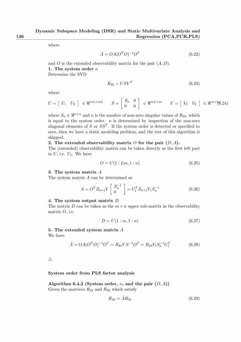
136Dynamic Subspace Modeling (DSR) and Static Multivariate Analysis and
Regression (PCA,PCR,PLS)
where
A = OA(OT O)−1OT (6.22)
and O is the extended observability matrix for the pair (A,D).1. The system order nDetermine the SVD
R32 = USV T (6.23)
where
U =[
U1 U2
] ∈ <mL×mL S =[
Sn 00 0
]∈ <mL×ni V =
[V1 V2
] ∈ <ni×ni(6.24)
where Sn ∈ <n×n and n is the number of non-zero singular values of R32, whichis equal to the system order. n is determined by inspection of the non-zerodiagonal elements of S or SST . If the system order is detected or specified tozero, then we have a static modeling problem, and the rest of this algorithm isskipped.2. The extended observability matrix O for the pair (D, A).The (extended) observability matrix can be taken directly as the first left partin U , i.e. U1. We have
O = U(1 : Lm, 1 : n) (6.25)
3. The system matrix AThe system matrix A can be determined as
A = OT Zk+1V
[S−1
n
0
]= UT
1 Zk+1V1S−1n (6.26)
4. The system output matrix DThe matrix D can be taken as the m×n upper sub-matrix in the observabilitymatrix O, i.e.
D = U(1 : m, 1 : n) (6.27)
5. The extended system matrix AWe have
A = OA(OT O)−1OT = R42V S−1OT = R42V1S−1n UT
1 (6.28)
4
System order from PLS factor analysis
Algorithm 6.4.2 (System order, n, and the pair (D,A))Given the matrices R42 and R32 which satisfy
R42 = AR32 (6.29)
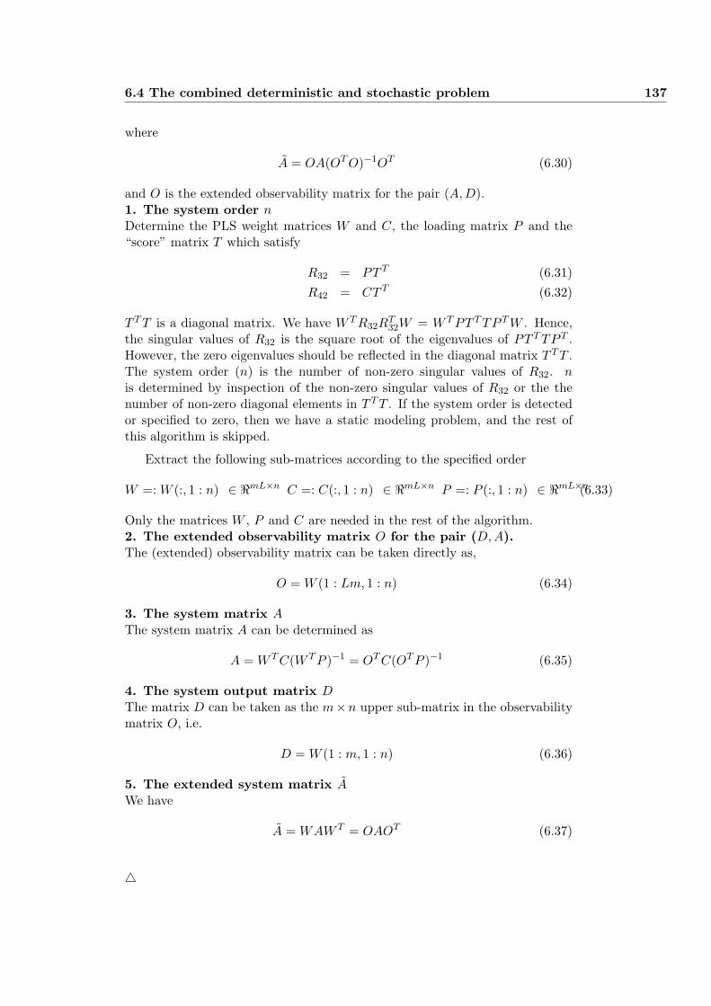
6.4 The combined deterministic and stochastic problem 137
where
A = OA(OT O)−1OT (6.30)
and O is the extended observability matrix for the pair (A,D).1. The system order nDetermine the PLS weight matrices W and C, the loading matrix P and the“score” matrix T which satisfy
R32 = PT T (6.31)R42 = CT T (6.32)
T T T is a diagonal matrix. We have W T R32RT32W = W T PT T TP T W . Hence,
the singular values of R32 is the square root of the eigenvalues of PT T TP T .However, the zero eigenvalues should be reflected in the diagonal matrix T T T .The system order (n) is the number of non-zero singular values of R32. nis determined by inspection of the non-zero singular values of R32 or the thenumber of non-zero diagonal elements in T T T . If the system order is detectedor specified to zero, then we have a static modeling problem, and the rest ofthis algorithm is skipped.
Extract the following sub-matrices according to the specified order
W =: W (:, 1 : n) ∈ <mL×n C =: C(:, 1 : n) ∈ <mL×n P =: P (:, 1 : n) ∈ <mL×n(6.33)
Only the matrices W , P and C are needed in the rest of the algorithm.2. The extended observability matrix O for the pair (D, A).The (extended) observability matrix can be taken directly as,
O = W (1 : Lm, 1 : n) (6.34)
3. The system matrix AThe system matrix A can be determined as
A = W T C(W T P )−1 = OT C(OT P )−1 (6.35)
4. The system output matrix DThe matrix D can be taken as the m×n upper sub-matrix in the observabilitymatrix O, i.e.
D = W (1 : m, 1 : n) (6.36)
5. The extended system matrix AWe have
A = WAW T = OAOT (6.37)
4
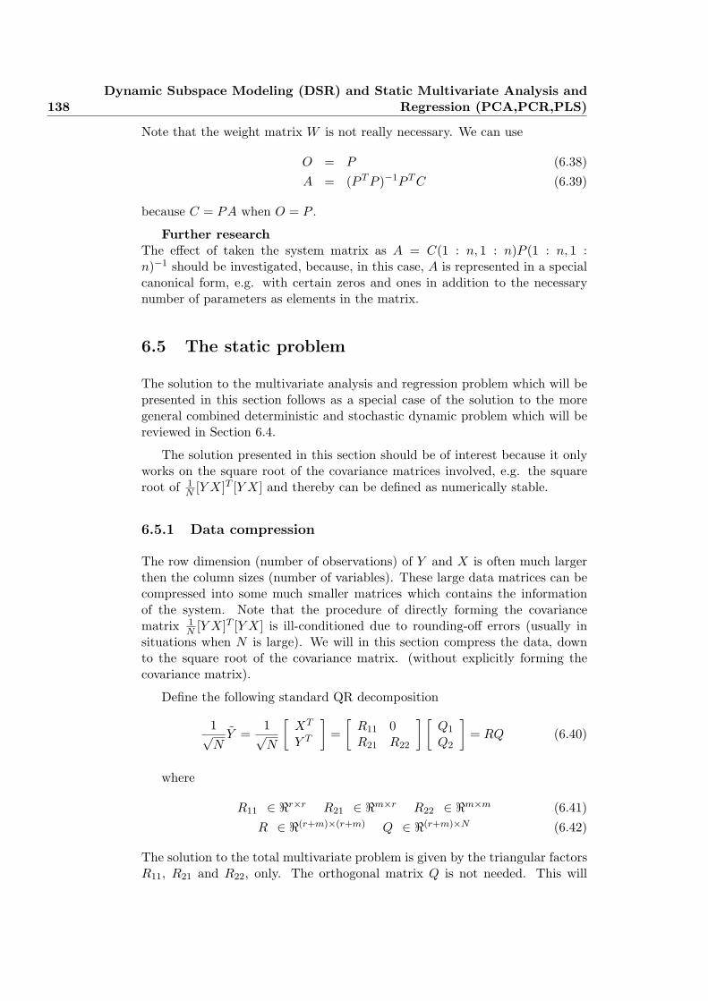
138Dynamic Subspace Modeling (DSR) and Static Multivariate Analysis and
Regression (PCA,PCR,PLS)
Note that the weight matrix W is not really necessary. We can use
O = P (6.38)A = (P T P )−1P T C (6.39)
because C = PA when O = P .
Further researchThe effect of taken the system matrix as A = C(1 : n, 1 : n)P (1 : n, 1 :n)−1 should be investigated, because, in this case, A is represented in a specialcanonical form, e.g. with certain zeros and ones in addition to the necessarynumber of parameters as elements in the matrix.
6.5 The static problem
The solution to the multivariate analysis and regression problem which will bepresented in this section follows as a special case of the solution to the moregeneral combined deterministic and stochastic dynamic problem which will bereviewed in Section 6.4.
The solution presented in this section should be of interest because it onlyworks on the square root of the covariance matrices involved, e.g. the squareroot of 1
N [Y X]T [Y X] and thereby can be defined as numerically stable.
6.5.1 Data compression
The row dimension (number of observations) of Y and X is often much largerthen the column sizes (number of variables). These large data matrices can becompressed into some much smaller matrices which contains the informationof the system. Note that the procedure of directly forming the covariancematrix 1
N [Y X]T [Y X] is ill-conditioned due to rounding-off errors (usually insituations when N is large). We will in this section compress the data, downto the square root of the covariance matrix. (without explicitly forming thecovariance matrix).
Define the following standard QR decomposition
1√N
Y =1√N
[XT
Y T
]=
[R11 0R21 R22
] [Q1
Q2
]= RQ (6.40)
where
R11 ∈ <r×r R21 ∈ <m×r R22 ∈ <m×m (6.41)R ∈ <(r+m)×(r+m) Q ∈ <(r+m)×N (6.42)
The solution to the total multivariate problem is given by the triangular factorsR11, R21 and R22, only. The orthogonal matrix Q is not needed. This will
6.5 The static problem 139
reduce the computational effort and storage considerably, especially when thenumber of observations N is large compared to the number of variables.
We have directly the following equation for the regression coefficients
R21 = BT R11 (6.43)
In order to solve this equation for B, standard PLS or PCR methods can beapplied.
6.5.2 The residual
The lower triangular matrix R22 is the square root of the residual covariancematrix. The covariance estimate of the noise (or residuals) is given by
∆ =1N
ET E = R22RT22 (6.44)
6.5.3 Effective rank analysis
The principal components
The lower triangular matrix R11 is the square root of the covariance matrix1N XT X. The singular values of R11 is equal to the square root of the eigen-values of 1
N XT X. Hence, the principal component analysis can be made bya singular value decomposition of R11. The number of principal componentsis the number of “non-zero” singular values of R11. The “non-zero” singularvalues are determined by inspection. We have
R11 = USV T =[
U1 U2
] [Sa 00 S0
] [V1 V2
]T (6.45)
The number of principal components a, is equal to the row size of Sa ∈ <a×a.S0 contains the zero singular values or singular values which are put to zero onthe diagonal. Hence
R11 = U1SaVT1 (6.46)
PLS factors
From an iterative procedure (e.g. by the Power method for computing eigen-values and eigenvectors) the PLS method compute the weight matrices W andC and the loading matrix P , and decomposes X and Y into
RT11 = TP T (6.47)
RT21 = TCT (6.48)
It is possible to determine r factors from the PLS algorithm corresponding tothe columns in W . The first factor and the first column in W is the maximum
140Dynamic Subspace Modeling (DSR) and Static Multivariate Analysis and
Regression (PCA,PCR,PLS)
eigenvalue and eigenvector of the covariance matrix 1N XT Y Y T X, respectively.
The effective rank index (a) is bounded by 1 ≤ a ≤ r. One idea is to estimatethe rank index as the number of “non-zero” PLS factors followed by crossvalidation. The “non-zero” factors are estimated by inspection.
6.5.4 Regression
The principal component regression
B = R11(RT11R11)−1RT
21 (6.49)B = (RT
11)−1RT
21 (6.50)
If the number of principal components is less than r, then, we are using thepseudo-inverse in the expressions for the regression matrix, i.e. we do not invertzero or almost zero singular values. Hence
BT = R21V1S−1a UT
1 (6.51)
PLS regression
The PLS regression is of the form
B = W (P T W )−1CT (6.52)
where the matrices W ∈ <r×a, P ∈ <r×a, C ∈ <m×a, results from the PLSalgorithm. Note that W T W = I.
6.6 Concluding remarks
A method for analyzing and modeling input and output relationships betweenvariables in possibly dynamical systems is presented. This method is viewedagainst methods such as PCR and PLS which are frequently used for modelingand analysis of static relationships between variables.
References
Di Ruscio, D. (1994). Methods for the identification of state space models frominput and output measurements. SYSID 94, The 10th IFAC Symposiumon System Identification, Copenhagen, July 4 - 6.
Di Ruscio, D. (1995a). A method for the identification of state space mod-els from input and output measurements. Modeling, Identification andControl, Vol.16 No. 3.

6.6 Concluding remarks 141
Di Ruscio, D. (1995b). A Method for Identification of Combined Determin-istic and Stochastic Systems: Robust implementation. Third EuropeanControl Conference ECC95, September 5-8, 1995.
Lindgren, F., Geladi, P. and S. Wold (1993). The kernal algorithm for PLS.Journal of chemometrics, Vol. 7, 45-59.

142Dynamic Subspace Modeling (DSR) and Static Multivariate Analysis and
Regression (PCA,PCR,PLS)

Chapter 7
On Subspace Identification ofthe Extended ObservabilityMatrix
7.1 Introduction
The lower Left Q-orthogonal (LQ) (or the Q-orthogonal, upper Right (QR))decomposition is used in order to compute certain projection matrices in theSubspace IDentification (SID) algorithms by Verhagen (1994), Van Overscheeand De Moor (1994) and Di Ruscio (1995), (1997). In this paper the PartialLeast Squares (PLS) method, Wold (1966), is used to compute the projectionmatrices. The PLS method is a simple alternative.
7.2 Definitions
7.2.1 Notation
The projection of (the row space of) a matrix A onto (the row space of) anothermatrix B is denoted A/B and defined as
A/Bdef= ABT (BBT )†B, (7.1)
where † denotes the Moore-Penrose pseudo-inverse. Also define
B⊥ def= I −BT (BBT )†B (7.2)
so that BB⊥ = 0. The projection of the row space of A onto the orthogonalcomplement of the row space of B is then AB⊥. Hence A is decomposed intotwo terms as
A = A/B + AB⊥, (7.3)
where the two matrix terms A/B and AB⊥ are orthogonal to each other.
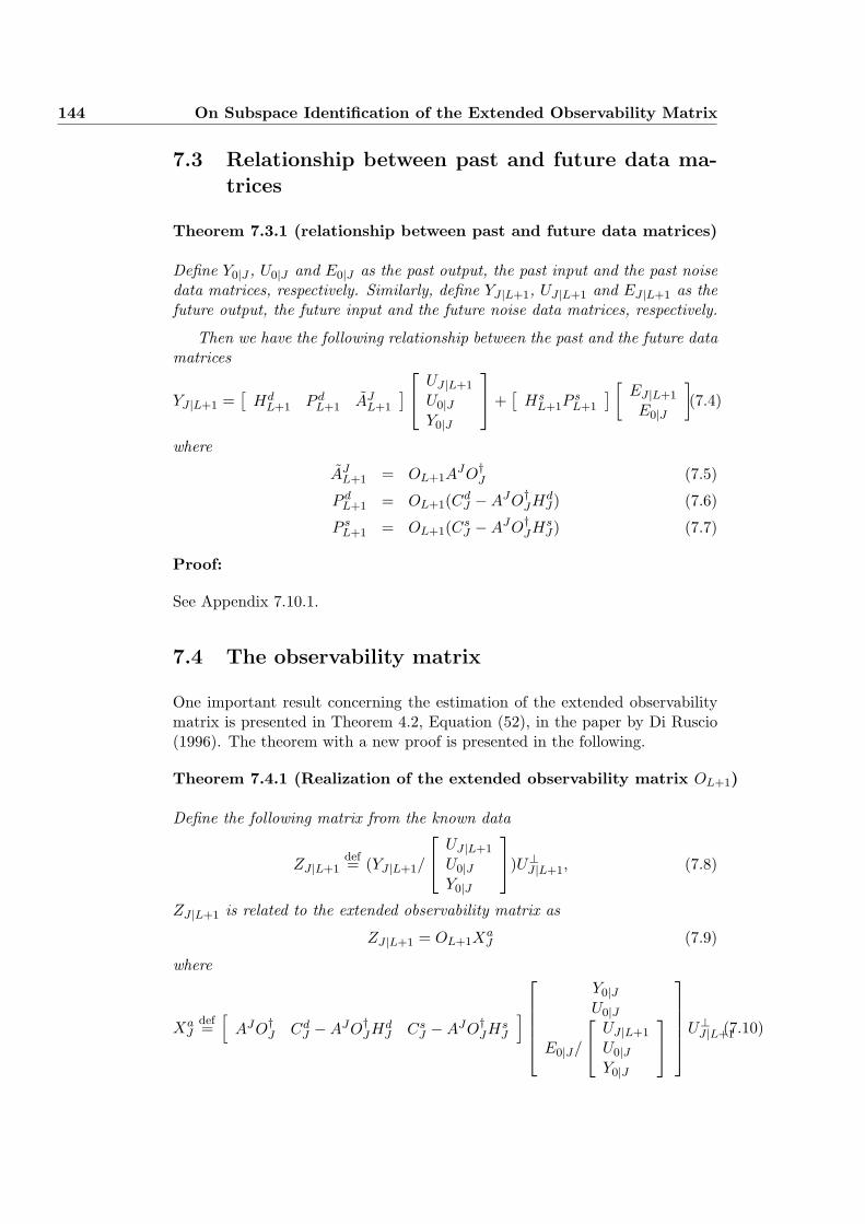
144 On Subspace Identification of the Extended Observability Matrix
7.3 Relationship between past and future data ma-trices
Theorem 7.3.1 (relationship between past and future data matrices)
Define Y0|J , U0|J and E0|J as the past output, the past input and the past noisedata matrices, respectively. Similarly, define YJ |L+1, UJ |L+1 and EJ |L+1 as thefuture output, the future input and the future noise data matrices, respectively.
Then we have the following relationship between the past and the future datamatrices
YJ |L+1 =[
HdL+1 P d
L+1 AJL+1
]
UJ |L+1
U0|JY0|J
+
[Hs
L+1PsL+1
] [EJ |L+1
E0|J
](7.4)
where
AJL+1 = OL+1A
JO†J (7.5)
P dL+1 = OL+1(Cd
J −AJO†JHd
J) (7.6)
P sL+1 = OL+1(Cs
J −AJO†JHs
J) (7.7)
Proof:
See Appendix 7.10.1.
7.4 The observability matrix
One important result concerning the estimation of the extended observabilitymatrix is presented in Theorem 4.2, Equation (52), in the paper by Di Ruscio(1996). The theorem with a new proof is presented in the following.
Theorem 7.4.1 (Realization of the extended observability matrix OL+1)
Define the following matrix from the known data
ZJ |L+1def= (YJ |L+1/
UJ |L+1
U0|JY0|J
)U⊥
J |L+1, (7.8)
ZJ |L+1 is related to the extended observability matrix as
ZJ |L+1 = OL+1XaJ (7.9)
where
XaJ
def=[
AJO†J Cd
J −AJO†JHd
J CsJ −AJO†
JHsJ
]
Y0|JU0|J
E0|J/
UJ |L+1
U0|JY0|J
U⊥J |L+1(7.10)
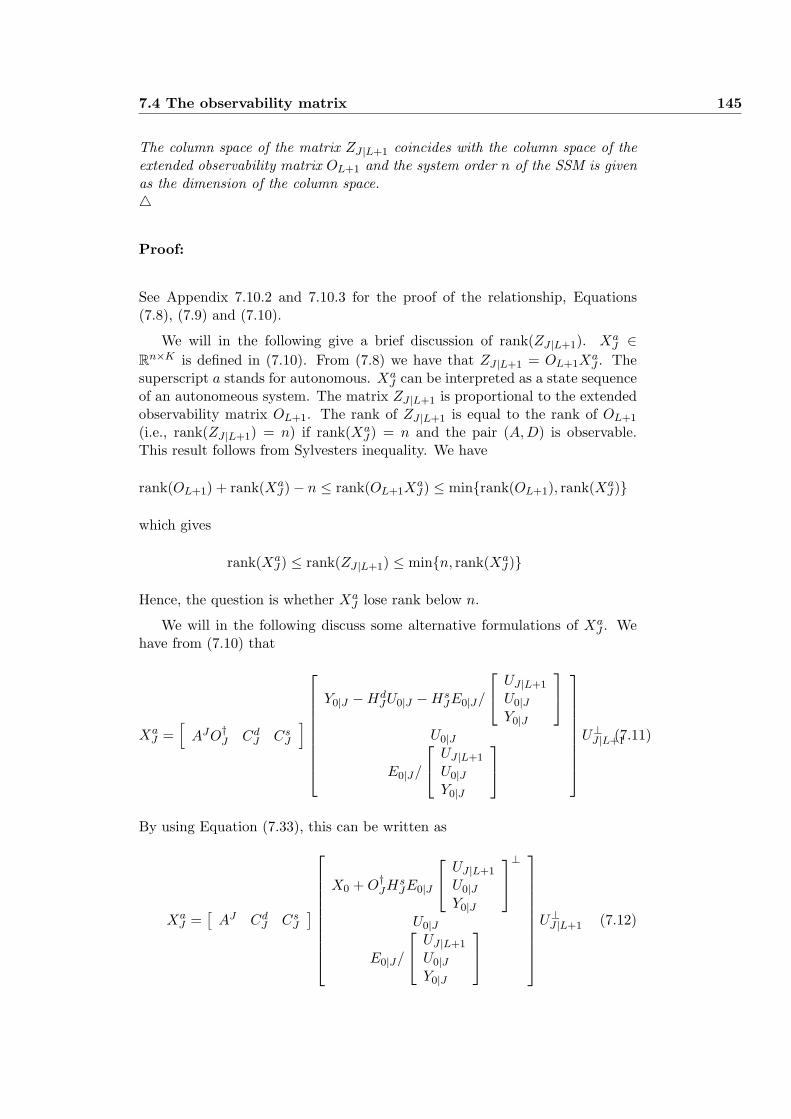
7.4 The observability matrix 145
The column space of the matrix ZJ |L+1 coincides with the column space of theextended observability matrix OL+1 and the system order n of the SSM is givenas the dimension of the column space.4
Proof:
See Appendix 7.10.2 and 7.10.3 for the proof of the relationship, Equations(7.8), (7.9) and (7.10).
We will in the following give a brief discussion of rank(ZJ |L+1). XaJ ∈
Rn×K is defined in (7.10). From (7.8) we have that ZJ |L+1 = OL+1XaJ . The
superscript a stands for autonomous. XaJ can be interpreted as a state sequence
of an autonomeous system. The matrix ZJ |L+1 is proportional to the extendedobservability matrix OL+1. The rank of ZJ |L+1 is equal to the rank of OL+1
(i.e., rank(ZJ |L+1) = n) if rank(XaJ) = n and the pair (A,D) is observable.
This result follows from Sylvesters inequality. We have
rank(OL+1) + rank(XaJ)− n ≤ rank(OL+1X
aJ) ≤ min{rank(OL+1), rank(Xa
J)}
which gives
rank(XaJ) ≤ rank(ZJ |L+1) ≤ min{n, rank(Xa
J)}
Hence, the question is whether XaJ lose rank below n.
We will in the following discuss some alternative formulations of XaJ . We
have from (7.10) that
XaJ =
[AJO†
J CdJ Cs
J
]
Y0|J −HdJU0|J −Hs
JE0|J/
UJ |L+1
U0|JY0|J
U0|J
E0|J/
UJ |L+1
U0|JY0|J
U⊥J |L+1(7.11)
By using Equation (7.33), this can be written as
XaJ =
[AJ Cd
J CsJ
]
X0 + O†JHs
JE0|J
UJ |L+1
U0|JY0|J
⊥
U0|J
E0|J/
UJ |L+1
U0|JY0|J
U⊥J |L+1 (7.12)
146 On Subspace Identification of the Extended Observability Matrix
An alternative description is found by using Equations (7.36) and (7.68)
XaJ =
[AJ Cd
J CsJ
]
X0/
UJ |L+1
U0|JY0|J
U0|J
E0|J/
UJ |L+1
U0|JY0|J
U⊥J |L+1 (7.13)
This expression relates XaJ to the reversed extended controllability matrices Cd
J
and CsJ for the pairs (A,B) and (A,C), respectively.
At this stage our statement is that rank(XaJ) = n if:
• the pair (A, [B,C]) is controllable,
• the states X0 is sufficiently correlated with the instruments (past inputsand outputs) U0|J and Y0|J ,
• the input is persistent exiting of a sufficient high order,
• the past noise E0|J is sufficiently correlated with the instruments (pastdata) U0|J and Y0|J .
We have the following special case results.
Lemma 7.4.1 Assume J →∞, K →∞, J(m+r) ≤ Lm and that A is stable.
Then
ZJ |L+1 = (YJ |L+1/
UJ |L+1
U0|JY0|J
)U⊥
J |L+1 =
OL+1
[Cd
J CsJ
]
U0|J
E0|J/
UJ |L+1
U0|JY0|J
U⊥
J |L+1
(7.14)
and
rank(ZJ |L+1) = n (7.15)
if and only if the pair A, [BC] is controllable.4
Still another description is found by using (7.34)
XaJ = (XJ + (AJO†
JHsJ − Cs
J)E0|J
UJ |L+1
U0|JY0|J
⊥
)U⊥J |L+1 (7.16)
7.4 The observability matrix 147
From (7.16) we have that XaJ = XJU⊥
J |L+1 when the system is deterministic.Hence, for a deterministic system rank(Xa
J) = n if the inputs are persistentlyexiting of a sufficiently high order.
A simple formulation can be found by using (7.33) and (7.67)
XaJ = XJ/
UJ |L+1
U0|JY0|J
U⊥
J |L+1 (7.17)
Using the definition of the projection A/B, and providing the inverse exist, anddefine the matrix of instruments as
W1 =[
U0|JY0|J
](7.18)
then we have
XaJ = XJU⊥
J |L+1WT1 (W1U
⊥J |L+1W
T1 )−1W1U
⊥J |L+1 (7.19)
The covariance can then be written as
1K − 1
XaJ(Xa
J)T =1
K − 1XJU⊥
J |L+1WT1 (W1U
⊥J |L+1W
T1 )−1W1U
⊥J |L+1X
TJ (7.20)
For purely deterministic systems or for systems with a large signal to noiseratio we have
1K − 1
XaJ(Xa
J)T =1
K − 1XJU⊥
J |L+1XTJ (7.21)
which is positive definite. The inputs has (partly) generated the states. Thestates is therefore sufficiently correlated with the inputs.
Note also that Equation (7.8) can be expressed as follows
ZJ |L+1def= (YJ |L+1/
[UJ |L+1
W1
])U⊥
J |L+1
= YJ |L+1U⊥J |L+1W
T1 (W1U
⊥J |L+1W
T1 )−1W1U
⊥J |L+1
= (YJ |L+1U⊥J |L+1)/(W1U
⊥J |L+1) (7.22)
when UJ |L+1UTJ |L+1 and W1U
⊥J |L+1W
T1 are non-singular matrices.
Proof:
See Appendix 7.10.4.
148 On Subspace Identification of the Extended Observability Matrix
7.5 Standard deviation of the estimates
The subspace methods DSR, CVA and MOESP are shown to compute con-sistent (pole) estimates. However, in some circumstances the estimates showsa larger variability (standard deviation) than the estimates from PEM. Thisproblem is addressed in this section.
N4SID (Van Overschee and De Moor (1995)) works in general only forwhite noise inputs. It is shown in Di Ruscio (1996a) that an extra projectionis needed in order for the N4SID algorithm to give consistent estimates in thecase of colored inputs. A robustified algorithm is presented in Van Overschee(1995). However, as we understand it, the ROBUST algorithm estimate thepoles similarly as the MOESP algorithm.
In the case of rich exiting input signals, e.g. such as many real world inputsand of course white noise inputs etc., the subspace methods DSR, CVA andMOESP computes pole estimates which is comparable with those from PEM,both with respect to bias and variance.
For poorly exciting input signals the variance of the subspace pole estimatesis often larger than the variance of the PEM pole estimates. See e.g. Viberg(1995).
It is therefore important to clarify the reason for the sensitivity of the esti-mates from subspace methods in the case of poorly exciting input signals. Thequestion of how we can influence upon and reduce the variance of the subspaceparameter estimates is important.
In order to improve the estimates in case of poorly exiting input signals wesuggest to investigate the following ideas.
1. PCR, PLS or some other form of regularization for computing the pro-jections and pseudo-inverse matrices.
2. Using regularization when computing the pseudo-inverse matrices.
3. Scaling
We will in the next section show how the Partial Least Squares (PLS) methodcan be used to compute the projection matrices.
7.6 PLS for computing the projections
The LQ decomposition is used in the SID algorithms by Verhagen (1994), VanOverschee and De Moor (1994) and Di Ruscio (1995), (1997).
In the following a new method for computing the projection matrices whichis based on the Partial Least Squares (PLS) method is presented. Based onnumerical examples, we have found that this method may reduce the variabilityof the pole estimates in case of poorly exciting input signals. The reason for this
7.6 PLS for computing the projections 149
is that the projection matrices are computed without computing the pseudo-inverse of badly conditioned matrices. This results is to our knowledge new.
For simplicity in the following, define
Ydef=
UJ |L+1
U0|JY0|J
∈ Rp×K (7.23)
where the number of rows in Y are p = (L + 1 + J)r + Jm.
A 1st PLS decomposition is computed as follows. The arguments to the PLSalgorithm are the data matrix of future outputs YJ |L+1 and the data matrix withpast inputs and outputs and future inputs Y . The PLS algorithm is iterative.The number of iterations is equal to the number of components a1 which isbounded by 1 ≤ a1 ≤ p. Normally, a1 can be chosen as the effective rank ofY . The problem of choosing the number of components should be discussed insome details.
We have the following decompositions
Y = PT + G (7.24)YJ |L+1 = CT + F (7.25)
where T ∈ Ra1×K is an orthonormal matrix, i.e., TT T = Ia1 , P ∈ Rp×a1 is aloading matrix for Y , C ∈ R(L+1)m×a1 is a loading matrix for YJ |L+1. G ∈ Rp×K
and F ∈ R(L+1)m×K are residual matrices.
It can be shown that the projection of the row space of YJ |L+1 onto the rowspace of Y is equal to
ZdJ |L+1
def= YJ |L+1/Y = CT (7.26)
We now have to remove the effect of future outputs from ZdJ |L+1 in order to
recover the extended observability matrix of the system. From (7.24) we havethat
UJ |L+1 = P1T + G1 (7.27)
where P1 ∈ R(L+1)r×a1 is equal to the first (L + 1)r rows in matrix P , similarlyG1 ∈ R(L+1)r×K is equal to the first (L + 1)r rows in the residual matrix G.
The projection of the row space of matrix ZdJ |L+1 onto the orthogonal com-
plement of the row space of UJ |L+1 can then be computed as
ZJ |L+1def= Zd
J |L+1U⊥J |L+1 = C − CP T
1 (P1PT1 )†P1 (7.28)
However, in case of a badly conditioned matrix P1PT1 a second PLS can be
computed with matrices C and P1 as arguments. We have the following decom-positions
P1 = P2T2 + G2 (7.29)C = C2T2 + F2 (7.30)
150 On Subspace Identification of the Extended Observability Matrix
where T2 ∈ Ra2×a1 is orthonormal. P2 ∈ R(L+1)r×a2 is a loading matrix forP1, C2 ∈ R(L+1)m×a2 is a loading matrix for C. G2 ∈ R(L+1)r×a1 and F2 ∈R(L+1)m×a1 are residual matrices. From this we have the alternative to (7.28)
ZJ |L+1def= Zd
J |L+1U⊥J |L+1 = C − C2T
T2 . (7.31)
The number of components a2 used to compute the 2nd PLS decompositionshould be bounded by 1 ≤ a2 ≤ a1.
Usually one can put a1 = rank(Y ) for the 1st PLS decomposition anda2 = rank(P1) for the 2nd PLS decomposition. In practical situations it maybe difficult to compute the (effective) rank.
One should note that the effect of choosing a1 and a2 smaller than theranks of Y and UJ |L+1, respectively, may be that the variance of the estimatesis reduced. However, a bias may be included in the estimates. The problem ofchoosing a1 and a2 is in general a trade off between bias and variance. This isa form of regularization.
Monte Carlo simulations shows that the estimates when choosing a1 = p anda1 = rank(Y ), i.e., choosing the number of components in the 1st PLS equal tothe row size of Y or equal to the rank, and using (7.28) gives approximately thesame results as using the LQ decomposition for computing the same projections.This will be illustrated in the next section. The effect of choosing a1 < rank(Y )is that a bias in general is introduced in the estimates, however, the variancemay be reduced.
7.7 Numerical example
The results from a Monte Carlo simulation of a MIMO system are illustratedin Figure (7.1). The number of components was chosen as a1 = rank(Y ) inthe PLS decomposition used to compute the matrix ZJ |L+1. The number ofsamples was N = 5000. The input signal was chosen as
ut =[
(sin( t14) + sin( t
7) + sin( t3))k1
(sin( t25) + sin( t
10) + sin( t5) + sin(t))k2
](7.32)
where k1 and k2 are positive scalar parameters. Our experience is that in caseof porely exiting input signals the parameter L in the DSR algorithm (whichis the number of block rows in the extended observability matrix and whichcan be interpreted as the horizon used to predict the number of states) shouldbe chosen as small as possible in order to reduce the variance of the estimates.For the DSR method we have the condition n ≤ Lm. For this example n = 3and m = 2. Hence, the smallest possible parameter is L = 2. The results fromthe DSR methods obtained from using both the LQ and PLS approaches areillustrated in Figure 7.1.
The results from the ROBUST method by Van Overschee (1995) is alsopresented in Figure 7.1. The parameter for the number of block rows in this
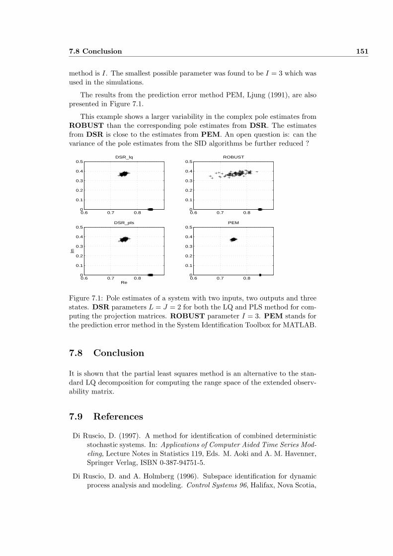
7.8 Conclusion 151
method is I. The smallest possible parameter was found to be I = 3 which wasused in the simulations.
The results from the prediction error method PEM, Ljung (1991), are alsopresented in Figure 7.1.
This example shows a larger variability in the complex pole estimates fromROBUST than the corresponding pole estimates from DSR. The estimatesfrom DSR is close to the estimates from PEM. An open question is: can thevariance of the pole estimates from the SID algorithms be further reduced ?
0.6 0.7 0.80
0.1
0.2
0.3
0.4
0.5DSR_lq
0.6 0.7 0.80
0.1
0.2
0.3
0.4
0.5ROBUST
0.6 0.7 0.80
0.1
0.2
0.3
0.4
0.5DSR_pls
Re
Im
0.6 0.7 0.80
0.1
0.2
0.3
0.4
0.5PEM
Figure 7.1: Pole estimates of a system with two inputs, two outputs and threestates. DSR parameters L = J = 2 for both the LQ and PLS method for com-puting the projection matrices. ROBUST parameter I = 3. PEM stands forthe prediction error method in the System Identification Toolbox for MATLAB.
7.8 Conclusion
It is shown that the partial least squares method is an alternative to the stan-dard LQ decomposition for computing the range space of the extended observ-ability matrix.
7.9 References
Di Ruscio, D. (1997). A method for identification of combined deterministicstochastic systems. In: Applications of Computer Aided Time Series Mod-eling, Lecture Notes in Statistics 119, Eds. M. Aoki and A. M. Havenner,Springer Verlag, ISBN 0-387-94751-5.
Di Ruscio, D. and A. Holmberg (1996). Subspace identification for dynamicprocess analysis and modeling. Control Systems 96, Halifax, Nova Scotia,
152 On Subspace Identification of the Extended Observability Matrix
May 1996.
Golub, G. H. and C. F. Van Loan (1983). Matrix Computations. North OxfordAcademic Publishers Ltd.
Larimore, W. E. (1983). System identification, reduced order filtering andmodeling via canonical variate analysis. Proc. of the American ControlConference, San Francisco, USA, pp. 445-451.
Larimore, W. E. (1990). Canonical Variate Analysis in Identification, Filteringand Adaptive Control. Proc. of the 29th Conference on Decision andControl, Honolulu, Hawaii, December 1990, pp. 596-604.
Ljung, L. (1991). System Identification Toolbox. The Mathworks, Inc.
Faurre, P. L. (1976). Stochastic realization algorithms. In: System Identifica-tion: Advances and Case Studies, (eds. R. K. Mehra and D. G. Lainiotis),Academic Press.
Kung, S. Y. (1978). A new identification and Model Reduction Algorithm viaSingular Value Decomposition. Conf. on Circuits, Systems and Comput-ers, Pacific Grove, CA, November 1978, pp. 705-714.
Moore, B. C. (1981). Principal Component Analysis in Linear Systems: Con-trollability, Observability, and Model Reduction. IEEE Trans. on Auto-matic Control, Vol. AC-26, pp. 17-31.
Van Overschee, P. and B. De Moor (1994). N4SID: Subspace Algorithms forthe Identification of Combined Deterministic Stochastic Systems. Auto-matica, vol. 30, No. 1, pp.75-94.
Van Overschee, P. (1995). Subspace Identification: theory-implementation-application. PhD thesis, Katholieke Universiteit Leuven, Belgium.
Van Overschee, P. and B. De Moor (1995). A Unifying Theorem for ThreeSubspace System Identification Algorithms. Automatica, vol. 31, No. 12,pp. 1853-1864.
Verhagen, M. (1994). Identification of the deterministic part of MIMO statespace models given on innovations form from input output data. Auto-matica, vol. 30, No. 1, pp. 61-74.
Viberg, M. (1995). Subspace-Based Methods for the Identification of LinearTime-invariant Systems. Automatica, vol. 31, No. 12, pp. 1835-1851.
Wold, H. (1966). Non-linear estimation by iterative least squares procedures.Researsch papers in statistics, Ed. David, F. Wiley, New York, pp. 411-444.
7.10 Appendix: proofs 153
7.10 Appendix: proofs
7.10.1 Proof of Equation (7.4)
We have
YJ |L+1 = OL+1XJ + HdL+1UJ |L+1 + Hs
L+1EJ |L+1 (7.33)
The relationship between the “future” sequence of states, XJ , and the “past”sequence of states, X0, is given by
XJ = AJX0 + CdJU0|J + Cs
JE0|J (7.34)
Substituting Equation (7.34) into equation (7.33) in order to eliminate XJ gives
YJ |L+1 = OL+1(AJX0 + CdJU0|J + Cs
JE0|J) + HdL+1UJ |L+1 + Hs
L+1EJ |L+1(7.35)
An expression for the sequence of past states, X0, is determined from
Y0|J = OJX0 + HdJU0|J + Hs
JE0|J (7.36)
Equation (7.36) gives
X0 = O†J(Y0|J −Hd
JU0|J −HsJE0|J) (7.37)
Substituting Equation (7.37) into Equation (7.35) in order to eliminate X0 gives
YJ |L+1 = OL+1AJO†
J(Y0|J −HdJU0|J −Hs
JE0|J) + OL+1CdJU0|J + OL+1C
sJE0|J
+ HdL+1UJ |L+1 + Hs
L+1EJ |L+1 (7.38)
which can be written as
YJ |L+1 = OL+1AJO†
JY0|J + (OL+1CdJ −OL+1A
JO†JHd
J)U0|J+ (OL+1C
sJ −OL+1A
JO†JHs
J)E0|J+ Hd
L+1UJ |L+1 + HsL+1EJ |L+1 (7.39)
which is identical to Equation (7.4), Theorem 7.3.1. QED.
154 On Subspace Identification of the Extended Observability Matrix
7.10.2 Proof I of Equation (7.10)
Projection I: (remove effect of future noise, EJ |L+1)From Equation (7.4) we have
YJ |L+1/
UJ |L+1
U0|JY0|J
=
[Hd
L+1 P dL+1 AJ
L+1
]
UJ |L+1
U0|JY0|J
+P sL+1E0|J/
UJ |L+1
U0|JY0|J
+ dE1 (7.40)
where
dE1def= Hs
L+1EJ |L+1/
UJ |L+1
U0|JY0|J
(7.41)
and
limK→∞
dE1 = HsL+1( lim
K→∞EJ |L+1/
UJ |L+1
U0|JY0|J
) = 0(L+1)m×K (7.42)
Rearranging the terms on the right hand side in Equation (7.40) gives
YJ |L+1/
UJ |L+1
U0|JY0|J
=
[P d
L+1 AJL+1 P s
L+1
]
U0|JY0|J
E0|J/
UJ |L+1
U0|JY0|J
+ HdL+1UJ |L+1 + dE1(7.43)
Projection II: (remove effect of future inputs, UJ |L+1)
(YJ |L+1/
UJ |L+1
U0|JY0|J
)U⊥
J |L+1 =
[P d
L+1 AL+1 P sL+1
]
U0|JY0|J
E0|J/
UJ |L+1
U0|JY0|J
U⊥J |L+1 + dE2 (7.44)
where
dE2def= dE1U
⊥J |L+1 (7.45)
Equation (7.44) is equal to Equation (7.10) in Theorem 7.4.1. Note thatlimK→∞ dE2 = 0(L+1)m×K . QED.
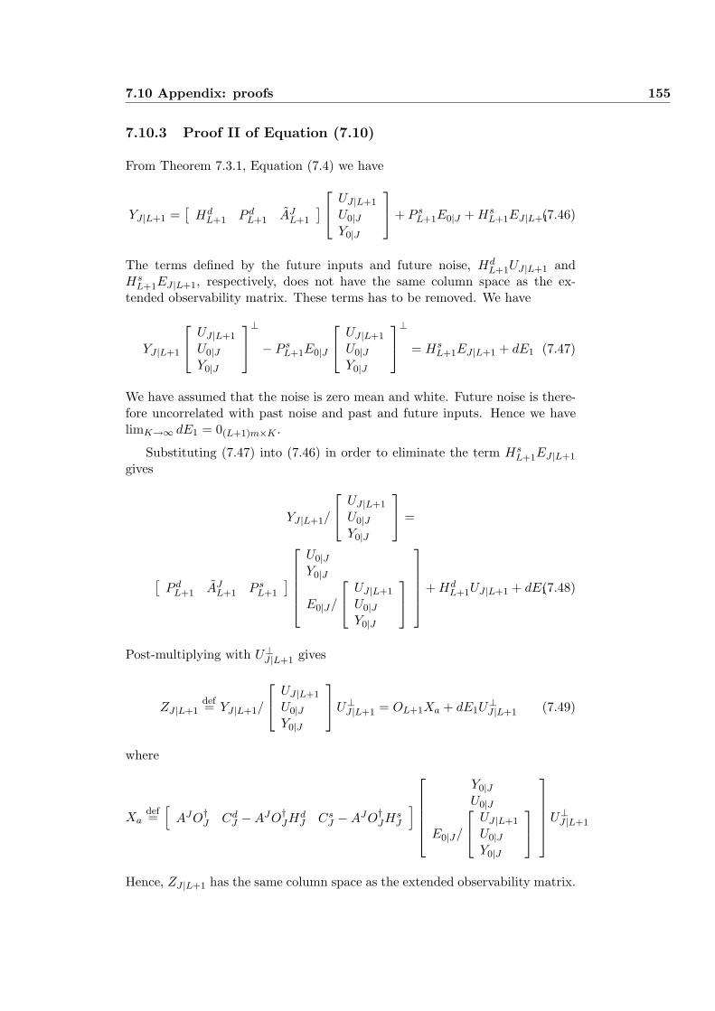
7.10 Appendix: proofs 155
7.10.3 Proof II of Equation (7.10)
From Theorem 7.3.1, Equation (7.4) we have
YJ |L+1 =[
HdL+1 P d
L+1 AJL+1
]
UJ |L+1
U0|JY0|J
+ P s
L+1E0|J + HsL+1EJ |L+1(7.46)
The terms defined by the future inputs and future noise, HdL+1UJ |L+1 and
HsL+1EJ |L+1, respectively, does not have the same column space as the ex-
tended observability matrix. These terms has to be removed. We have
YJ |L+1
UJ |L+1
U0|JY0|J
⊥
− P sL+1E0|J
UJ |L+1
U0|JY0|J
⊥
= HsL+1EJ |L+1 + dE1 (7.47)
We have assumed that the noise is zero mean and white. Future noise is there-fore uncorrelated with past noise and past and future inputs. Hence we havelimK→∞ dE1 = 0(L+1)m×K .
Substituting (7.47) into (7.46) in order to eliminate the term HsL+1EJ |L+1
gives
YJ |L+1/
UJ |L+1
U0|JY0|J
=
[P d
L+1 AJL+1 P s
L+1
]
U0|JY0|J
E0|J/
UJ |L+1
U0|JY0|J
+ HdL+1UJ |L+1 + dE1(7.48)
Post-multiplying with U⊥J |L+1 gives
ZJ |L+1def= YJ |L+1/
UJ |L+1
U0|JY0|J
U⊥
J |L+1 = OL+1Xa + dE1U⊥J |L+1 (7.49)
where
Xadef=
[AJO†
J CdJ −AJO†
JHdJ Cs
J −AJO†JHs
J
]
Y0|JU0|J
E0|J/
UJ |L+1
U0|JY0|J
U⊥J |L+1
Hence, ZJ |L+1 has the same column space as the extended observability matrix.
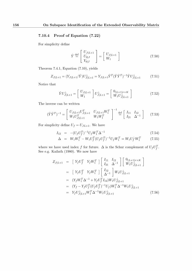
156 On Subspace Identification of the Extended Observability Matrix
7.10.4 Proof of Equation (7.22)
For simplicity define
Ydef=
UJ |L+1
U0|JY0|J
=
[UJ |L+1
W1
](7.50)
Theorem 7.4.1, Equation (7.10), yields
ZJ |L+1 = (YJ |L+1/Y )U⊥J |L+1 = YJ |L+1Y
T (Y Y T )−1Y U⊥J |L+1 (7.51)
Notice that
Y U⊥J |L+1 =
[UJ |L+1
W1
]U⊥
J |L+1 =[
0(L+1)r×K
W1U⊥J |L+1
](7.52)
The inverse can be written
(Y Y T )−1 =
[UJ |L+1U
TJ |L+1 UJ |L+1W
T1
W1UTJ |L+1 W1W
T1
]−1def=
[I11 I12
I21 ∆−1
](7.53)
For simplicity define Uf = UJL+1. We have
I12 = −(UfUTf )−1UfW T
1 ∆−1 (7.54)
∆ = W1WT1 −W1U
Tf (UfUT
f )−1UfW T1 = W1U
⊥f W T
1 (7.55)
where we have used index f for future. ∆ is the Schur complement of UfUTf .
See e.g. Kailath (1980). We now have
ZJ |L+1 =[
YfUTf YfW T
1
] [I11 I12
I21 ∆−1
] [0(L+1)r×K
W1U⊥J |L+1
]
=[
YfUTf YfW T
1
] [I12
∆−1
]W1U
⊥J |L+1
= (YfW T1 ∆−1 + YfUT
f I12)W1U⊥J |L+1
= (Yf − YfUTf (UfUT
f )−1Uf )W T1 ∆−1W1U
⊥J |L+1
= YfU⊥J |L+1W
T1 ∆−1W1U
⊥J |L+1 (7.56)
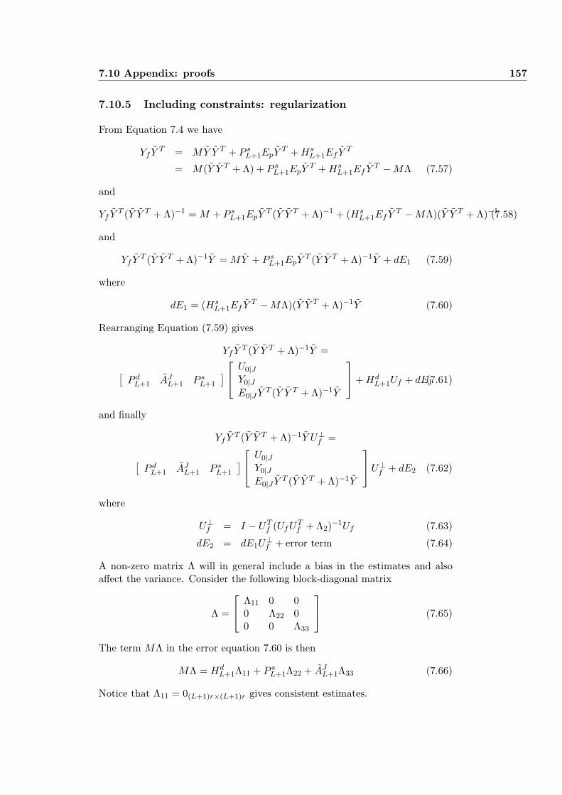
7.10 Appendix: proofs 157
7.10.5 Including constraints: regularization
From Equation 7.4 we have
Yf Y T = MY Y T + P sL+1EpY
T + HsL+1Ef Y T
= M(Y Y T + Λ) + P sL+1EpY
T + HsL+1Ef Y T −MΛ (7.57)
and
Yf Y T (Y Y T + Λ)−1 = M + P sL+1EpY
T (Y Y T + Λ)−1 + (HsL+1Ef Y T −MΛ)(Y Y T + Λ)−1(7.58)
and
Yf Y T (Y Y T + Λ)−1Y = MY + P sL+1EpY
T (Y Y T + Λ)−1Y + dE1 (7.59)
where
dE1 = (HsL+1Ef Y T −MΛ)(Y Y T + Λ)−1Y (7.60)
Rearranging Equation (7.59) gives
Yf Y T (Y Y T + Λ)−1Y =
[P d
L+1 AJL+1 P s
L+1
]
U0|JY0|JE0|J Y T (Y Y T + Λ)−1Y
+ Hd
L+1Uf + dE1(7.61)
and finally
Yf Y T (Y Y T + Λ)−1Y U⊥f =
[P d
L+1 AJL+1 P s
L+1
]
U0|JY0|JE0|J Y T (Y Y T + Λ)−1Y
U⊥
f + dE2 (7.62)
where
U⊥f = I − UT
f (UfUTf + Λ2)−1Uf (7.63)
dE2 = dE1U⊥f + error term (7.64)
A non-zero matrix Λ will in general include a bias in the estimates and alsoaffect the variance. Consider the following block-diagonal matrix
Λ =
Λ11 0 00 Λ22 00 0 Λ33
(7.65)
The term MΛ in the error equation 7.60 is then
MΛ = HdL+1Λ11 + P s
L+1Λ22 + AJL+1Λ33 (7.66)
Notice that Λ11 = 0(L+1)r×(L+1)r gives consistent estimates.
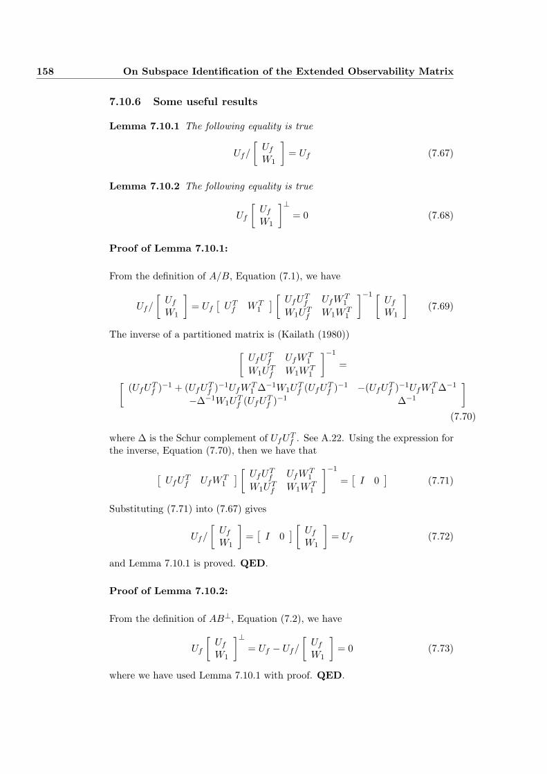
158 On Subspace Identification of the Extended Observability Matrix
7.10.6 Some useful results
Lemma 7.10.1 The following equality is true
Uf/
[Uf
W1
]= Uf (7.67)
Lemma 7.10.2 The following equality is true
Uf
[Uf
W1
]⊥= 0 (7.68)
Proof of Lemma 7.10.1:
From the definition of A/B, Equation (7.1), we have
Uf/
[Uf
W1
]= Uf
[UT
f W T1
] [UfUT
f UfW T1
W1UTf W1W
T1
]−1 [Uf
W1
](7.69)
The inverse of a partitioned matrix is (Kailath (1980))
[UfUT
f UfW T1
W1UTf W1W
T1
]−1
=
[(UfUT
f )−1 + (UfUTf )−1UfW T
1 ∆−1W1UTf (UfUT
f )−1 −(UfUTf )−1UfW T
1 ∆−1
−∆−1W1UTf (UfUT
f )−1 ∆−1
]
(7.70)
where ∆ is the Schur complement of UfUTf . See A.22. Using the expression for
the inverse, Equation (7.70), then we have that
[UfUT
f UfW T1
] [UfUT
f UfW T1
W1UTf W1W
T1
]−1
=[
I 0]
(7.71)
Substituting (7.71) into (7.67) gives
Uf/
[Uf
W1
]=
[I 0
] [Uf
W1
]= Uf (7.72)
and Lemma 7.10.1 is proved. QED.
Proof of Lemma 7.10.2:
From the definition of AB⊥, Equation (7.2), we have
Uf
[Uf
W1
]⊥= Uf − Uf/
[Uf
W1
]= 0 (7.73)
where we have used Lemma 7.10.1 with proof. QED.
7.10 Appendix: proofs 159
7.10.7 Proof III of Equation (7.10)
The ESSM constructed from future data is
YJ+1|L = ALYJ |L + BLUJ |L+1 + CLEJ |L+1 (7.74)
Using Lemma 7.10.1 we get
ZdJ+1|L = ALZd
J |L + BLUJ |L+1 + CLdEJ |L+1 (7.75)
where
ZdJ+1|L
def= YJ+1|L/
UJ |L+1
U0|JY0|J
(7.76)
ZdJ |L
def= YJ |L/
UJ |L+1
U0|JY0|J
(7.77)
dEJ |L+1def= EJ |L+1/
UJ |L+1
U0|JY0|J
(7.78)
Due to assumptions (ergodic noise process) the error term dEJ |L+1 tends tozero w.p.1 as the number of columns K tends to infinity.
Hence,
(A,B, D,E) = arg minA,B,D,E
‖ ZdJ+1|L − AZd
J |L − BUJ |L+1 ‖F (7.79)
7.10.8 Prediction of future outputs
We have the following relationship
YJ |L+1 = ZdJ |L+1 + Zs
J |L+1 (7.80)
From Theorem 4.3, Di Ruscio (1997), we have that the innovations can beestimated from
FEJ+L|1 = ZsJ+L|1(Z
sJ |L)⊥ (7.81)
from the above we have that a predictor for the future outputs is given by
yJ+L|1 = ZdJ+L|1(Z
sJ |L)⊥ (7.82)
This indicates that
yJ+L|1 = YJ+L|1(ZsJ |L)⊥ (7.83)
The predictor can simply be written
yJ+L|1 = ZdJ+L|1 (7.84)

160 On Subspace Identification of the Extended Observability Matrix
Chapter 8
Subspace identification of thestates and the Kalman filtergain
8.1 Introduction
A complete subspace identification (SID) algorithm are discussed and derivedin this paper. The derivation presented is different from the other published pa-pers on subspace identification, Van Overschee and De Moor (1994), Larimore(1990), Viberg (1995) and Van Overschee (1995) and the references therein,because we are using general input and output matrix equations which de-scribes the relationship between the past and the future input and output datamatrices.
One of the contributions in this paper is that it is shown that the Kalmanfilter model matrices, including the Kalman gain and the noise innovationsprocess, of a combined deterministic and stochastic system can be identifieddirectly from certain projection matrices which are computed from the knowninput and output data, without solving any Riccati or Lyapunov matrix equa-tions. This subspace method and results was presented without proof in DiRuscio (1995) and Di Ruscio (1997). One contribution in this paper is a com-plete derivation with proof. A new method for computing the matrices in thedeterministic part of the system is presented. This method has been used inthe DSR Toolbox for Matlab, Di Ruscio (1996), but has not been publishedearlier.
Furthermore, it is pointed out that the states, in general (i.e. for coloredinput signals), only can be computed if the complete deterministic part of themodel is known or identified first. This is probably the reason for which the statebased subspace algorithms which are presented in the literature does not workproperly for colored input signals. The SID algorithm in Verhagen (1994) worksfor colored input signals. The stochastic part of the model is not computed by
162 Subspace identification of the states and the Kalman filter gain
this algorithm. The N4SID algorithm in Van Overschee and De Moor (1994)works well and only for white input signals. The stochastic part of the model iscomputed by solving a Riccati equation. However, the robust modification inVan Overschee and De Moor (1995) works well also for colored input signals.
The rest of this paper is organized as follows. Some basic matrix definitionsand notations are presented in Section 8.2. The problem of subspace identi-fication of the states for both colored and white input signals is discussed inSection 8.3.1. The subspace identification of the extended observability matrix,which possibly is the most important step in any SID algorithm, are discussedin Section 8.3.2. It is proved that the Kalman filter gain matrix and the noiseinnovations process can be identified directly from the data in Section 8.3.3.A least squares optimal method for computing the deterministic part of thecombined deterministic and stochastic system is presented in Section 8.3.4.
The problem of using subspace methods for closed loop systems are pointedout and some solutions to the problem are pointed out in section 8.4.
The main contribution in this paper is a new method for subspace systemidentification that works for closed loop as well as open loop systems. Themethod are based on the theory in Section 3 and is presented in Section 8.5.This method is probably one of the best for closed loop subspace system iden-tification.
Some topics and remarks related to the algorithm are presented in Section8.6. Numerical examples are provided in Section 8.7 in order to illustrate thebehaviour of the algorithm both in open and closed loop. Some concludingremarks follows in Section 8.8.
8.2 Notation and definitions
8.2.1 System and matrix definitions
Consider the following state space model on innovations form
xk+1 = Axk + Buk + Cek, (8.1)yk = Dxk + Euk + Fek, (8.2)
where ek is white noise with covariance matrix E(ekeTk ) = Im. One of the
problems addressed and discussed in this paper is to directly identify (subspaceidentification) the system order, n, the state vector xk ∈ Rn, and the matrices(A,B, C,D, E, F ) from a sequence of known input and output data vectors, uk,∈ Rr and yk, ∈ Rm, respectively. A structure parameter, g, is introduced sothat g = 1 when E is to be identified and g = 0 when E is a-priori knownto be zero. This should be extended to a structure matrix G with ones andzeroes, the ones pointing to the elements in E which are to be estimated. Thisis not considered further here. Based on (8.1) and (8.2) we make the followingdefinitions for further use:
8.2 Notation and definitions 163
Definition 8.1 (Basic matrix definitions)The extended observability matrix, Oi, for the pair (D, A) is defined as
Oidef=
DDA...DAi−1
∈ Rim×n, (8.3)
where the subscript i denotes the number of block rows.
The reversed extended controllability matrix, Cdi , for the pair (A,B) is
defined as
Cdi
def=[
Ai−1B Ai−2B · · · B] ∈ Rn×ir, (8.4)
where the subscript i denotes the number of block columns. A reversed extendedcontrollability matrix, Cs
i , for the pair (A,C) is defined similar to (8.4), i.e.,
Csi
def=[
Ai−1C Ai−2C · · · C] ∈ Rn×im, (8.5)
i.e., with B substituted with C in (8.4). The lower block triangular Toeplitzmatrix, Hd
i , for the quadruple matrices (D, A, B,E)
Hdi
def=
E 0m×r 0m×r · · · 0m×r
DB E 0m×r · · · 0m×r
DAB DB E · · · 0m×r...
......
. . ....
DAi−2B DAi−3B DAi−4B · · · E
∈ Rim×(i+g−1)r, (8.6)
where the subscript i denotes the number of block rows and i + g − 1 is thenumber of block columns. Where 0m×r denotes the m × r matrix with zeroes.A lower block triangular Toeplitz matrix Hs
i for the quadruple (D, A, C, F ) isdefined as
Hsi
def=
F 0m×m 0m×m · · · 0m×m
DC F 0m×m · · · 0m×m
DAC DC F · · · 0m×m...
......
. . ....
DAi−2C DAi−3C DAi−4C · · · F
∈ Rim×im. (8.7)
8.2.2 Hankel matrix notation
Hankel matrices are frequently used in realization theory and subspace sys-tem identification. The special structure of a Hankel matrix as well as somematching notations, which are frequently used througout, are defined in thefollowing.
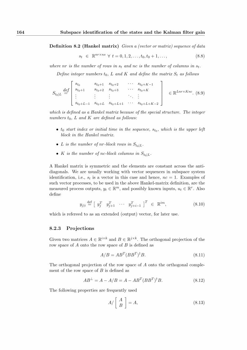
164 Subspace identification of the states and the Kalman filter gain
Definition 8.2 (Hankel matrix) Given a (vector or matrix) sequence of data
st ∈ Rnr×ns ∀ t = 0, 1, 2, . . . , t0, t0 + 1, . . . , (8.8)
where nr is the number of rows in st and nc is the number of columns in st.
Define integer numbers t0, L and K and define the matrix St as follows
St0|Ldef=
st0 st0+1 st0+2 · · · st0+K−1
st0+1 st0+2 st0+3 · · · st0+K...
......
. . ....
st0+L−1 st0+L st0+L+1 · · · st0+L+K−2
∈ RLnr×Knc. (8.9)
which is defined as a Hankel matrix because of the special structure. The integernumbers t0, L and K are defined as follows:
• t0 start index or initial time in the sequence, st0, which is the upper leftblock in the Hankel matrix.
• L is the number of nr-block rows in St0|L.
• K is the number of nc-block columns in St0|L.
A Hankel matrix is symmetric and the elements are constant across the anti-diagonals. We are usually working with vector sequences in subspace systemidentification, i.e., st is a vector in this case and hence, nc = 1. Examples ofsuch vector processes, to be used in the above Hankel-matrix definition, are themeasured process outputs, yt ∈ Rm, and possibly known inputs, ut ∈ Rr. Alsodefine
yj|idef=
[yT
j yTj+1 · · · yT
j+i−1
]T ∈ Rim, (8.10)
which is refereed to as an extended (output) vector, for later use.
8.2.3 Projections
Given two matrices A ∈ Ri×k and B ∈ Rj×k. The orthogonal projection of therow space of A onto the row space of B is defined as
A/B = ABT (BBT )†B. (8.11)
The orthogonal projection of the row space of A onto the orthogonal comple-ment of the row space of B is defined as
AB⊥ = A−A/B = A−ABT (BBT )†B. (8.12)
The following properties are frequently used
A/
[AB
]= A, (8.13)
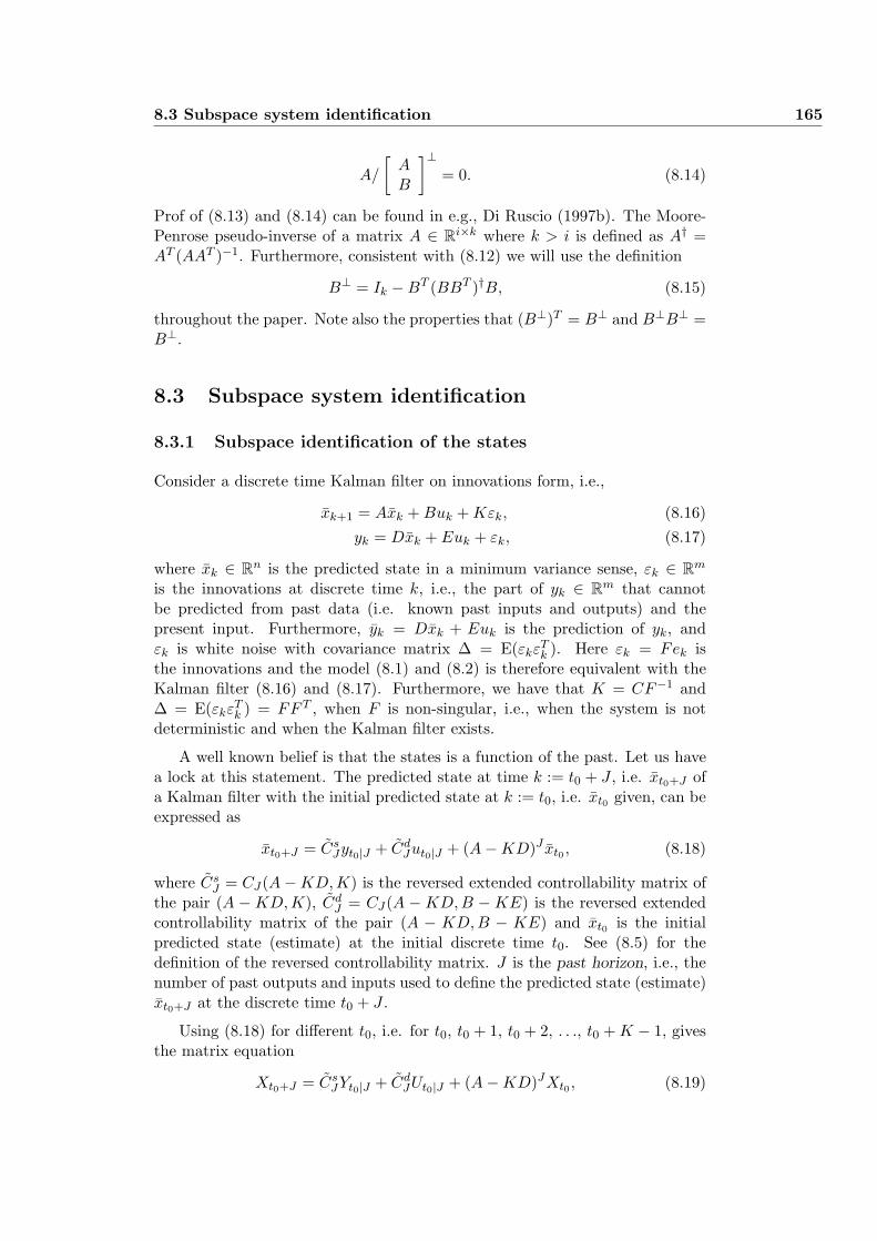
8.3 Subspace system identification 165
A/
[AB
]⊥= 0. (8.14)
Prof of (8.13) and (8.14) can be found in e.g., Di Ruscio (1997b). The Moore-Penrose pseudo-inverse of a matrix A ∈ Ri×k where k > i is defined as A† =AT (AAT )−1. Furthermore, consistent with (8.12) we will use the definition
B⊥ = Ik −BT (BBT )†B, (8.15)
throughout the paper. Note also the properties that (B⊥)T = B⊥ and B⊥B⊥ =B⊥.
8.3 Subspace system identification
8.3.1 Subspace identification of the states
Consider a discrete time Kalman filter on innovations form, i.e.,
xk+1 = Axk + Buk + Kεk, (8.16)yk = Dxk + Euk + εk, (8.17)
where xk ∈ Rn is the predicted state in a minimum variance sense, εk ∈ Rm
is the innovations at discrete time k, i.e., the part of yk ∈ Rm that cannotbe predicted from past data (i.e. known past inputs and outputs) and thepresent input. Furthermore, yk = Dxk + Euk is the prediction of yk, andεk is white noise with covariance matrix ∆ = E(εkε
Tk ). Here εk = Fek is
the innovations and the model (8.1) and (8.2) is therefore equivalent with theKalman filter (8.16) and (8.17). Furthermore, we have that K = CF−1 and∆ = E(εkε
Tk ) = FF T , when F is non-singular, i.e., when the system is not
deterministic and when the Kalman filter exists.
A well known belief is that the states is a function of the past. Let us havea lock at this statement. The predicted state at time k := t0 + J , i.e. xt0+J ofa Kalman filter with the initial predicted state at k := t0, i.e. xt0 given, can beexpressed as
xt0+J = CsJyt0|J + Cd
Jut0|J + (A−KD)J xt0 , (8.18)
where CsJ = CJ(A−KD, K) is the reversed extended controllability matrix of
the pair (A −KD,K), CdJ = CJ(A −KD, B −KE) is the reversed extended
controllability matrix of the pair (A − KD,B − KE) and xt0 is the initialpredicted state (estimate) at the initial discrete time t0. See (8.5) for thedefinition of the reversed controllability matrix. J is the past horizon, i.e., thenumber of past outputs and inputs used to define the predicted state (estimate)xt0+J at the discrete time t0 + J .
Using (8.18) for different t0, i.e. for t0, t0 + 1, t0 + 2, . . ., t0 + K − 1, givesthe matrix equation
Xt0+J = CsJYt0|J + Cd
JUt0|J + (A−KD)JXt0 , (8.19)
166 Subspace identification of the states and the Kalman filter gain
where
Xt0+J =[
xt0+J xt0+J+1 · · · xt0+J+K−1
] ∈ Rn×K , (8.20)
Xt0 =[
xt0 xt0+1 · · · xt0+K−1
] ∈ Rn×K . (8.21)
where K is the number of columns in the data matrices. Note that K also isequal to the number of vector equations of the form (8.18) which is used toform the matrix version (8.19). Note also that the state matrix Xt0 can beeliminated from (8.19) by using the relationship
Yt0|J = OJXt0 + HdJUt0|J+g−1 + Hs
JEt0|J , (8.22)
which we have deduced from the innovations form, state space model (8.1) and(8.2). Putting t0 =: t0 + J in (8.22) gives
Yt0+J |L = OLXt0+J + HdLUt0+J |L+g−1 + Hs
LEt0+J |L. (8.23)
Using (8.19) to eliminate Xt0+J in (8.23) gives a matrix equation which re-lates the future data matrices Yt0+J |L, Ut0+J |L+g−1, Et0+J |L and the past datamatrices Yt0|J , Ut0|J , Et0|J .
The data is usually defined at time instant (or number of observations)k = 1, 2, . . . , N . Hence, t0 = 1 in this case. However, we are often definingt0 = 0 which corresponds to data defined at k = 0, 1, . . . , N − 1. The bar usedto indicate predicted state is often omitted. Hence, for simplicity of notation,we define the following equations from (8.19), (8.22) and (8.23),
Y0|J = OJX0 + HdJU0|J+g−1 + Hs
JE0|J , (8.24)
XJ = CsJY0|J + Cd
JU0|J + (A−KD)JX0, (8.25)
YJ |L = OLXJ + HdLUJ |L+g−1 + Hs
LEJ |L, (8.26)
for lather use. Furthermore, (8.26) and (8.25) gives
YJ |L =[
HdL OLCd
J OLCsJ
]
UJ |L+g−1
U0|JY0|J
+ OL(A−KD)JX0 + Hs
LEJ |L.
(8.27)
Equation (8.27) is important for understanding a SID algorithm, because, itgives the relationship between the past and the future. Note also the termsin (8.27) which are ”proportional” with the extended observability matrix OL.From (8.27) we see that the effect from the future inputs, UJ |L+g−1, and thefuture noise, EJ |L, have to be removed from the future outputs, YJ |L, in orderto recover the subspace spanned by the extended observability matrix, OL. Avariation of this equation, in which the term X0 is eliminated by using (8.22)
8.3 Subspace system identification 167
or (8.24) is presented in Di Ruscio (1997b). Note also that (8.25) and (8.24)gives
XJ =[
P uJ P y
J
] [U0|JY0|J
]− P e
JE0|J , (8.28)
P uJ = Cd
J − (A−KD)JO†JHd
J , (8.29)
P yJ = Cs
J + (A−KD)JO†J , (8.30)
P eJ = (A−KD)JO†
JHsJ , (8.31)
where we for the sake of simplicity and without loss of generality have putg = 1. Equation (8.28) is useful because it shows that the future states XJ
is in the range of a matrix consisting of past inputs, U0|J , and past outputs,Y0|J (in the deterministic case or when J →∞). Note that we have introducedthe notation, P u
J , in order to represent the influence from the past inputs uponthe future. Combining (8.28) and (8.26) gives an alternative to (8.27), i.e. the”past-future” matrix equation,
YJ |L =[
HdL OLP u
J OLP yJ
]
UJ |L+g−1
U0|JY0|J
−OLP e
JE0|J + HsLEJ |L. (8.32)
The two last terms in (8.32) cannot be predicted from data, i.e., because E0|Jand EJ |L are built from the innovations process ek.
It is important to note that a consistent estimate of the system dynamicscan be obtained by choosing L and N properly. Choosing Lmin ≤ L whereLmin = n+rank(D)−1 and letting N →∞, is in general, necessary conditionsfor a consistent estimate of the dynamics. See Section 8.3.2 for further details.
On the other side, it is in general, also necessary to let J → ∞ in order toobtain a consistent estimate of the states. The reason for this is that the term(A−KD)J = 0 in this case. Hence, the effect of the initial state matrix X0 onthe future states XJ has died out. We have the following Lemma
Lemma 8.3.1 (Subspace identification of the states)Let K →∞ in the data matrices. The projected state matrix is defined as
XJ/
UJ |L+g−1
U0|JY0|J
= O†
L(
ZdJ|L︷ ︸︸ ︷
YJ |L/
UJ |L+g−1
U0|JY0|J
−Hd
LUJ |L+g−1)
= CsJY0|J + Cd
JU0|J + (A−KD)JX0/
UJ |L+g−1
U0|JY0|J
.
(8.33)
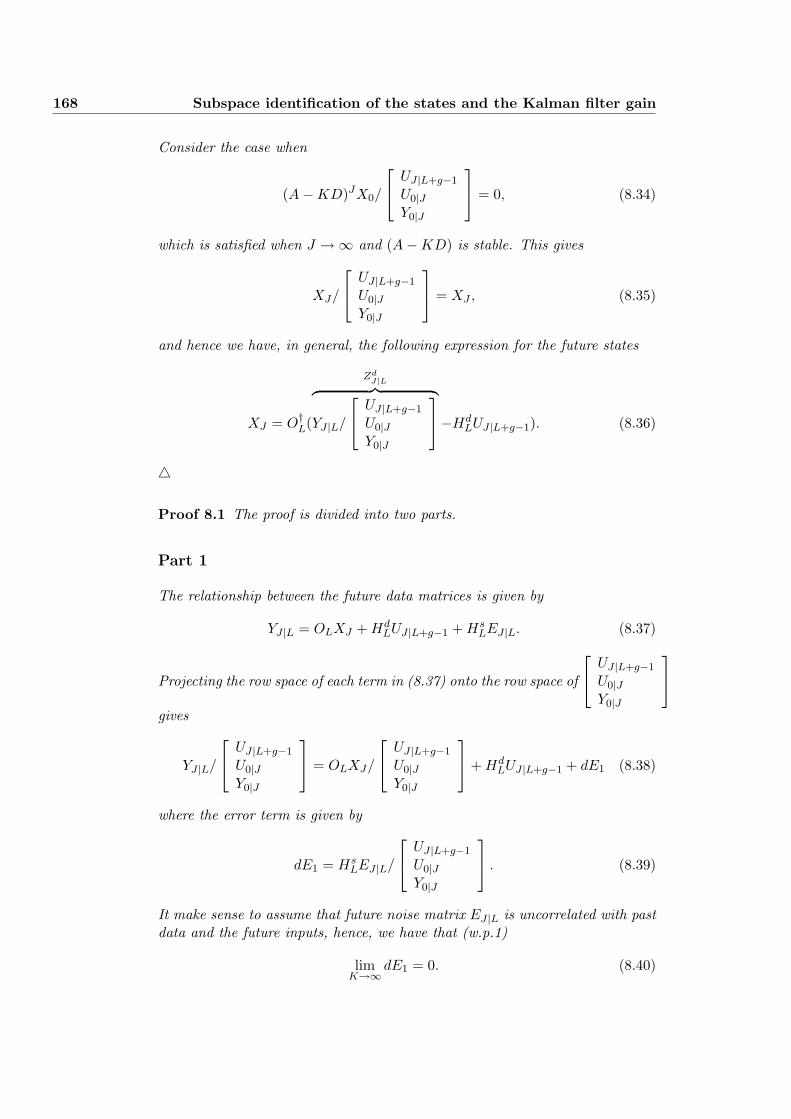
168 Subspace identification of the states and the Kalman filter gain
Consider the case when
(A−KD)JX0/
UJ |L+g−1
U0|JY0|J
= 0, (8.34)
which is satisfied when J →∞ and (A−KD) is stable. This gives
XJ/
UJ |L+g−1
U0|JY0|J
= XJ , (8.35)
and hence we have, in general, the following expression for the future states
XJ = O†L(
ZdJ|L︷ ︸︸ ︷
YJ |L/
UJ |L+g−1
U0|JY0|J
−Hd
LUJ |L+g−1). (8.36)
4
Proof 8.1 The proof is divided into two parts.
Part 1
The relationship between the future data matrices is given by
YJ |L = OLXJ + HdLUJ |L+g−1 + Hs
LEJ |L. (8.37)
Projecting the row space of each term in (8.37) onto the row space of
UJ |L+g−1
U0|JY0|J
gives
YJ |L/
UJ |L+g−1
U0|JY0|J
= OLXJ/
UJ |L+g−1
U0|JY0|J
+ Hd
LUJ |L+g−1 + dE1 (8.38)
where the error term is given by
dE1 = HsLEJ |L/
UJ |L+g−1
U0|JY0|J
. (8.39)
It make sense to assume that future noise matrix EJ |L is uncorrelated with pastdata and the future inputs, hence, we have that (w.p.1)
limK→∞
dE1 = 0. (8.40)
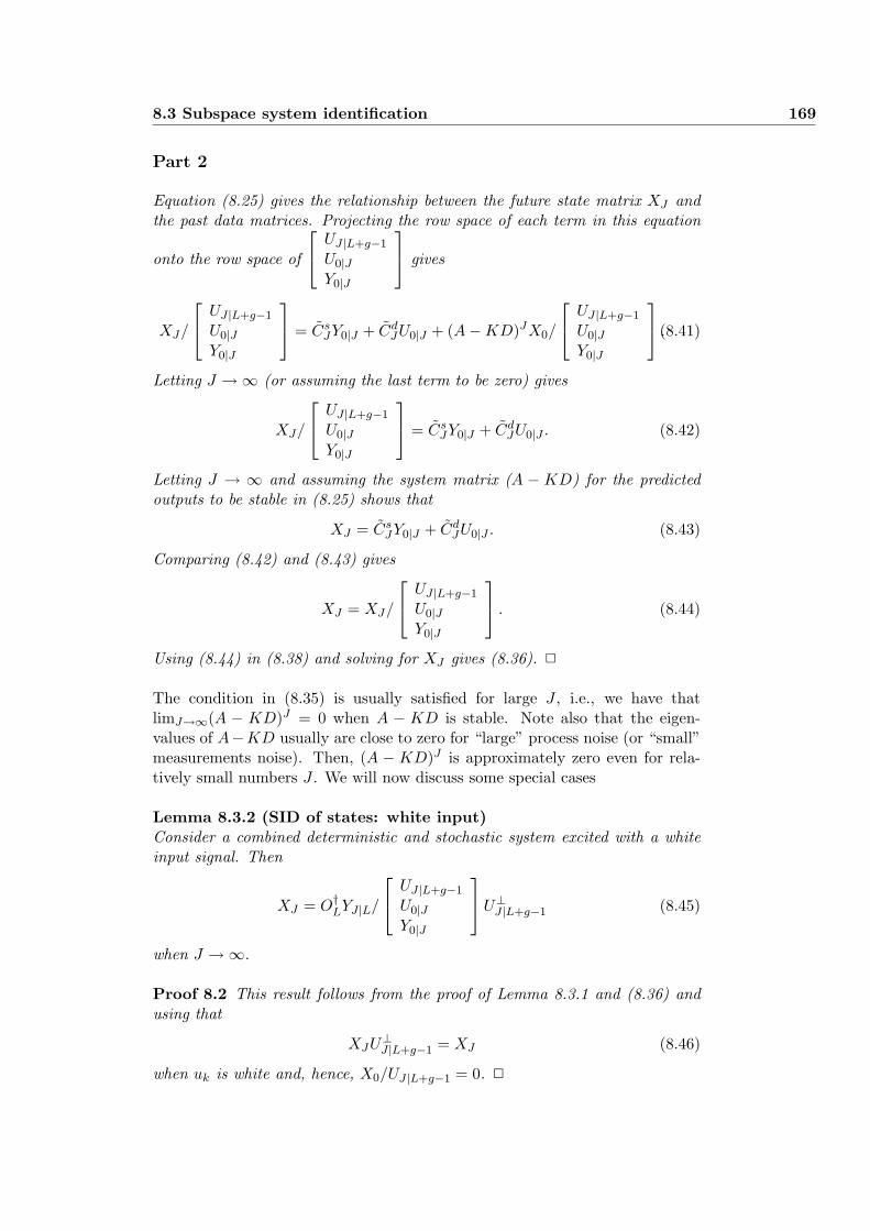
8.3 Subspace system identification 169
Part 2
Equation (8.25) gives the relationship between the future state matrix XJ andthe past data matrices. Projecting the row space of each term in this equation
onto the row space of
UJ |L+g−1
U0|JY0|J
gives
XJ/
UJ |L+g−1
U0|JY0|J
= Cs
JY0|J + CdJU0|J + (A−KD)JX0/
UJ |L+g−1
U0|JY0|J
.(8.41)
Letting J →∞ (or assuming the last term to be zero) gives
XJ/
UJ |L+g−1
U0|JY0|J
= Cs
JY0|J + CdJU0|J . (8.42)
Letting J → ∞ and assuming the system matrix (A − KD) for the predictedoutputs to be stable in (8.25) shows that
XJ = CsJY0|J + Cd
JU0|J . (8.43)
Comparing (8.42) and (8.43) gives
XJ = XJ/
UJ |L+g−1
U0|JY0|J
. (8.44)
Using (8.44) in (8.38) and solving for XJ gives (8.36). 2
The condition in (8.35) is usually satisfied for large J , i.e., we have thatlimJ→∞(A − KD)J = 0 when A − KD is stable. Note also that the eigen-values of A−KD usually are close to zero for “large” process noise (or “small”measurements noise). Then, (A − KD)J is approximately zero even for rela-tively small numbers J . We will now discuss some special cases
Lemma 8.3.2 (SID of states: white input)Consider a combined deterministic and stochastic system excited with a whiteinput signal. Then
XJ = O†LYJ |L/
UJ |L+g−1
U0|JY0|J
U⊥
J |L+g−1 (8.45)
when J →∞.
Proof 8.2 This result follows from the proof of Lemma 8.3.1 and (8.36) andusing that
XJU⊥J |L+g−1 = XJ (8.46)
when uk is white and, hence, X0/UJ |L+g−1 = 0. 2

170 Subspace identification of the states and the Kalman filter gain
Lemma 8.3.3 (SID of states: pure stochastic system)Consider a stochastic system. Then we simply have that
XJ = O†LYJ |L/Y0|J (8.47)
when J →∞ or when (A−KD)JX0/Y0|J = 0 is satisfied.
Proof 8.3 This result follows from the proof of Lemma 8.3.1 by putting themeasured input variables equal to zero. 2
Lemma 8.3.1 shows that it is in general (i.e. for colored input signals)necessary to know the deterministic part of the system, i.e., the Toepliz matrixHd
L in (8.36), in order to properly identify the states. This means that thematrices B and E in addition to D and A has to be identified prior to computingthe states. I.e. we need to know the deterministic part of the model. However,a special case is given by Lemma 8.3.2 and Equation (8.45) which shows thatthe states can be identified directly when the input signals is white. Note alsothat the extended observability matrix OL is needed in (8.36) and (8.45). OL
can be identified directly from the data. This is proved in the next Section8.3.2, and this is indeed the natural step in a SID algorithm.
In the case of a white input signal or when J →∞ then, HdL, and the state
matrix, XJ , can be computed as by the N4SID algorithm, Van Overschee andDe Moor (1996). From (8.32) and (8.28) we have the following lemma
Lemma 8.3.4 (States, XJ , and Toepliz matrix HdL: N4SID)
The following LS solution
[Hd
L OLP uJ OLP y
J
]= YJ |L
UJ |L+g−1
U0|JY0|J
†
+ dE. (8.48)
holds in:
i) The deterministic case, provided the input is PE of order J +L+g−1. Theerror term, dE = 0, in this case.
ii) When J → ∞, and the input is PE of infinite order. The error term,dE = 0, in this case.
iii) A white uk gives a consistent estimate of HdL irrespective of J > 0. How-
ever, OLP uJ and OLP y
J are not consistent estimates in this case. The firstmL× (L + g)r part of the error term, dE, is zero in this case.
Hence, under conditions i) and ii), OLP uJ and OLP y
J can be computed as in(8.48). Then the states can be consistently estimated as
XJ = O†L
[OLP u
J OLP yJ
] [U0|JY0|J
], (8.49)
provided conditions i) and ii) are satisfied, and O†L is known.
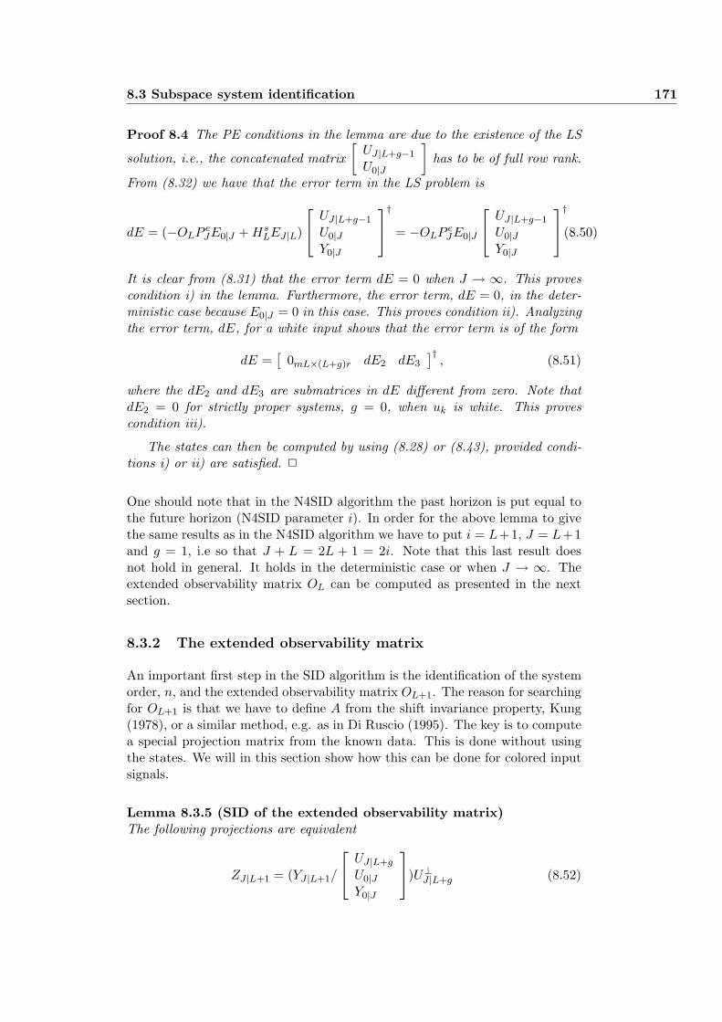
8.3 Subspace system identification 171
Proof 8.4 The PE conditions in the lemma are due to the existence of the LS
solution, i.e., the concatenated matrix[
UJ |L+g−1
U0|J
]has to be of full row rank.
From (8.32) we have that the error term in the LS problem is
dE = (−OLP eJE0|J + Hs
LEJ |L)
UJ |L+g−1
U0|JY0|J
†
= −OLP eJE0|J
UJ |L+g−1
U0|JY0|J
†
.(8.50)
It is clear from (8.31) that the error term dE = 0 when J → ∞. This provescondition i) in the lemma. Furthermore, the error term, dE = 0, in the deter-ministic case because E0|J = 0 in this case. This proves condition ii). Analyzingthe error term, dE, for a white input shows that the error term is of the form
dE =[
0mL×(L+g)r dE2 dE3
]†, (8.51)
where the dE2 and dE3 are submatrices in dE different from zero. Note thatdE2 = 0 for strictly proper systems, g = 0, when uk is white. This provescondition iii).
The states can then be computed by using (8.28) or (8.43), provided condi-tions i) or ii) are satisfied. 2
One should note that in the N4SID algorithm the past horizon is put equal tothe future horizon (N4SID parameter i). In order for the above lemma to givethe same results as in the N4SID algorithm we have to put i = L+1, J = L+1and g = 1, i.e so that J + L = 2L + 1 = 2i. Note that this last result doesnot hold in general. It holds in the deterministic case or when J → ∞. Theextended observability matrix OL can be computed as presented in the nextsection.
8.3.2 The extended observability matrix
An important first step in the SID algorithm is the identification of the systemorder, n, and the extended observability matrix OL+1. The reason for searchingfor OL+1 is that we have to define A from the shift invariance property, Kung(1978), or a similar method, e.g. as in Di Ruscio (1995). The key is to computea special projection matrix from the known data. This is done without usingthe states. We will in this section show how this can be done for colored inputsignals.
Lemma 8.3.5 (SID of the extended observability matrix)The following projections are equivalent
ZJ |L+1 = (YJ |L+1/
UJ |L+g
U0|JY0|J
)U⊥
J |L+g (8.52)
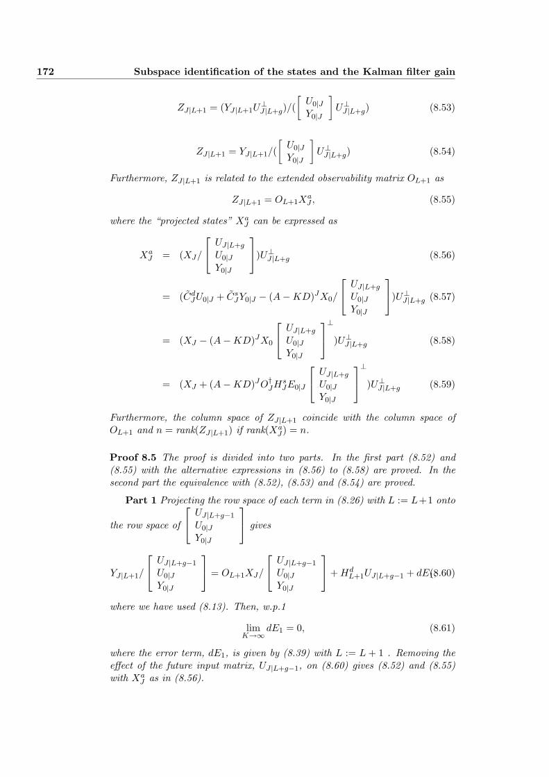
172 Subspace identification of the states and the Kalman filter gain
ZJ |L+1 = (YJ |L+1U⊥J |L+g)/(
[U0|JY0|J
]U⊥
J |L+g) (8.53)
ZJ |L+1 = YJ |L+1/([
U0|JY0|J
]U⊥
J |L+g) (8.54)
Furthermore, ZJ |L+1 is related to the extended observability matrix OL+1 as
ZJ |L+1 = OL+1XaJ , (8.55)
where the “projected states” XaJ can be expressed as
XaJ = (XJ/
UJ |L+g
U0|JY0|J
)U⊥
J |L+g (8.56)
= (CdJU0|J + Cs
JY0|J − (A−KD)JX0/
UJ |L+g
U0|JY0|J
)U⊥
J |L+g (8.57)
= (XJ − (A−KD)JX0
UJ |L+g
U0|JY0|J
⊥
)U⊥J |L+g (8.58)
= (XJ + (A−KD)JO†JHs
JE0|J
UJ |L+g
U0|JY0|J
⊥
)U⊥J |L+g (8.59)
Furthermore, the column space of ZJ |L+1 coincide with the column space ofOL+1 and n = rank(ZJ |L+1) if rank(Xa
J) = n.
Proof 8.5 The proof is divided into two parts. In the first part (8.52) and(8.55) with the alternative expressions in (8.56) to (8.58) are proved. In thesecond part the equivalence with (8.52), (8.53) and (8.54) are proved.
Part 1 Projecting the row space of each term in (8.26) with L := L+1 onto
the row space of
UJ |L+g−1
U0|JY0|J
gives
YJ |L+1/
UJ |L+g−1
U0|JY0|J
= OL+1XJ/
UJ |L+g−1
U0|JY0|J
+ Hd
L+1UJ |L+g−1 + dE1,(8.60)
where we have used (8.13). Then, w.p.1
limK→∞
dE1 = 0, (8.61)
where the error term, dE1, is given by (8.39) with L := L + 1 . Removing theeffect of the future input matrix, UJ |L+g−1, on (8.60) gives (8.52) and (8.55)with Xa
J as in (8.56).
8.3 Subspace system identification 173
Furthermore, projecting the row space of each term in (8.25) onto the row
space of
UJ |L+g−1
U0|JY0|J
gives
XJ/
UJ |L+g−1
U0|JY0|J
= Cs
JY0|J + CdJU0|J + (A−KD)JX0/
UJ |L+g−1
U0|JY0|J
(8.62)
From (8.25) we have that
CsJY0|J + Cd
JU0|J = XJ − (A−KD)JX0. (8.63)
Combining (8.60), (8.62) and (8.63) gives (8.52) and (8.57)-(8.58).
Part 2 It is proved in Di Ruscio (1997) that
ZJ |L+1 = YJ |L+1/
[UJ |L+g
W
]U⊥
J |L+g
= YJ |L+1U⊥J |L+gW
T (WU⊥J |L+gW
T )−1WU⊥J |L+g, (8.64)
where
W =[
U0|JY0|J
]. (8.65)
Using that U⊥J |L+gU
⊥J |L+g = U⊥
J |L+g in (8.64) proves the equivalence between(8.53), (8.54) and (8.52). 2
Lemma 8.3.6 (Consistency: Stochastic and deterministic systems)Let J →∞, then
ZJ |L+1 = OL+1XJU⊥J |L+g, (8.66)
where ZJ |L+1 is defined as in Lemma 8.3.5. A sufficient condition for consis-tency, and that OL+1 is contained in the column space of ZJ |L+1, is that thereare no pure state feedback.
Proof 8.6 Letting J → ∞ in (8.58) gives (8.66). This can also be provedby using (8.44) in (8.56). Furthermore, if there are pure state feedback thenXJU⊥
J |L+g will lose rank below the normal rank which is n. 2
Lemma 8.3.7 (Deterministic systems)For pure deterministic systems we have that (8.66) can be changed to
ZJ |L+1 =: YJ |L+1U⊥J |L+g = OL+1XJU⊥
J |L+g. (8.67)
The extended observability matrix OL+1 can be computed from the column spaceof YJ |L+1U
⊥J |L+g. Furthermore, one can let J = 0 in the deterministic case.
174 Subspace identification of the states and the Kalman filter gain
Proof 8.7 This follows from (8.66) and Lemma 8.3.5 by excluding the projec-tion which removes the noise. 2
Lemma 8.3.8 (Stochastic systems)For pure stochastic systems we have that (8.66) can be changed to
ZJ |L+1 =: YJ |L+1/Y0|J = OL+1XJ . (8.68)
The extended observability matrix OL+1 can be computed from the column spaceof YJ |L+1/Y0|J .
Proof 8.8 This follows from (8.66) and Lemma 8.3.5 by excluding the inputmatrices from the equations and definitions. 2
8.3.3 Identification of the stochastic subsystem
We will in this section prove that, when the extended observability matrix isknown (from Section 8.3.2), the kalman filter gain matrix can be identifieddirectly from the data. Furthermore, it is proved that the noise innovationsprocess can be identified directly in a first step in the DSR subspace algorithm.This result was first presented in Di Ruscio (1995) without proof. Some resultsconcerning this is also presented in Di Ruscio (2001) and (2003).
Lemma 8.3.9 (The innovations)Define the following projection from the data
ZsJ |L+1 = YJ |L+1 − YJ |L+1/
UJ |L+g
U0|JY0|J
= YJ |L+1
UJ |L+g
U0|JY0|J
⊥
. (8.69)
Then w.p.1 as J →∞Zs
J |L+1 = HsL+1EJ |L+1. (8.70)
Hence, the Toeplitz matrix HsL+1 (with Markov matrices F , DC, . . ., DAL−1C)
for the stochastic subsystem is in the column space of 1√K
ZsJ |L+1 since 1
K EJ |L+1ETJ |L+1 =
IL+1×L+1.
Proof 8.9 The relationship between the future data matrices is given by
YJ |L = OLXJ + HdLUJ |L+g−1 + Hs
LEJ |L. (8.71)
Projecting the row space of each term in (8.71) onto the row space of
UJ |L+g−1
U0|JY0|J
gives
YJ |L/
UJ |L+g−1
U0|JY0|J
= OLXJ/
UJ |L+g−1
U0|JY0|J
+ Hd
LUJ |L+g−1 + dE1, (8.72)
8.3 Subspace system identification 175
then, w.p.1
limK→∞
dE1 = 0, (8.73)
where dE1 is given in (8.39). Furthermore,
limJ→∞
XJ/
UJ |L+g−1
U0|JY0|J
= XJ , (8.74)
where we have used Equations (8.44) and (8.38). From (8.71), (8.72) and(8.74) we have that
YJ |L − YJ |L/
UJ |L+g−1
U0|JY0|J
= Hs
LEJ |L. (8.75)
Putting L := L + 1 in (8.75) gives (8.69). 2
Note the following from Lemma 3.9. The innovations can be identifieddirectly as for g = 1
ZsJ |1 = FEJ |1 = YJ |1 − YJ |1/
UJ |1U0|JY0|J
(8.76)
or for g = 0 when E = 0
ZsJ |1 = FEJ |1 = YJ |1 − YJ |1/
[U0|JY0|J
](8.77)
One should note that (8.77) holds for both open and closed loop systems. Forclosed loop systems it make sense to only consider systems in which the directfeed-through matrix, E, from the input uk to the output yk is zero. This resultwill be used in order to construct a subspace algorithm whic gives consistenresults for close loop systems, se Section 5.
It is now possible to directly identify the matrices C and F in the innovationsmodel (8.1) and (8.2) and K and ∆ in the Kalman filter (8.16) and (8.17). Twomethods are presented in the following. The first one is a direct covariancebased method for computing K and ∆ and the second one is a more numericallyreliable “square root” based method for computing C and F .
Lemma 8.3.10 (correlation method for K and ∆) Define the projectionmatrix Zs
J |L+1 as in (8.69) and define the correlation matrix
∆L+1 =1K
ZsJ |L+1(Z
sJ |L+1)
T = HsL+1(H
sL+1)
T . (8.78)
176 Subspace identification of the states and the Kalman filter gain
where the Toepliz matrix HsL+1 can be partitioned as
HsL+1 =
[F 0m×Lm
OLC HsL
], (8.79)
where C = KF . Hence, (8.78) can be written as
∆L+1 =[
∆11 ∆12
∆21 ∆22
]=
[FF T F (OLC)T
OLCF T OLC(OLC)T + HsL(Hs
L)T
]. (8.80)
From this we have
E(εkεTk ) = FF T = ∆11 (8.81)
and
K = CF−1 = O†L∆21∆−1
11 . (8.82)
Lemma 8.3.11 (square-root method for C and F ) The LQ decompositionof 1√
KZs
J |L+1 gives
1√K
ZsJ |L+1 = R33Q3. (8.83)
Then, the Toeplitz matrix HsL+1, and the Markov matrices F , DC, . . ., DAL−1C,
are given directly by
HsL+1 = R33. (8.84)
F can be taken as one of the diagonal m ×m block matrices in R33, e.g. thelower left sub-matrix, i.e.
F = R33(Lm + 1 : (L + 1)m,Lm + 1 : (L + 1)m), (8.85)
or as the mean of all the diagionals. Furthermore,
OLC = R33(m + 1 : (L + 1)m, 1 : m). (8.86)
The system matrix C is given by
C = O†LOLC = O†
LR33(m + 1 : (L + 1)m, 1 : m). (8.87)
The Kalman filter gain matrix and the innovations covariance matrix are givenby
K = CF−1 (8.88)
= O†LR33(m + 1 : (L + 1)m, 1 : m)R−1
33 (Lm + 1 : (L + 1)m,Lm + 1 : (L + 1)m)∆ = FF T . (8.89)
8.3 Subspace system identification 177
8.3.4 SID of the deterministic subsystem
The parameters in the B and E matrices can be computed from an optimalleast squares problem. A solution to this is given in the following
Lemma 8.3.12 (Extended state space model)The states can be eliminated from the state space model (8.1) and (8.2) to yieldthe so called Extended State Space Model (ESSM)
YJ+1|L = ALYJ |L + BLUJ |L+g + CLEJ |L+1, (8.90)
where
ALdef= OLA(OT
LOL)−1OTL ∈ RLm×Lm, (8.91)
BLdef=
[OLB Hd
L
]− AL
[Hd
L 0Lm×r
] ∈ RLm×(L+g)r, (8.92)
CLdef=
[OLC Hs
L
]− AL
[Hs
L 0Lm×m
] ∈ RLm×(L+1)m. (8.93)
Proof 8.10 Putting J =: J + 1 in (8.37) and substituting XJ+1 = AXJ +BUJ + CEJ into this equation gives
YJ+1|L = OLAXJ +[
OLB HdL
]UJ |L+g +
[OLC Hs
L
]EJ |L+1. (8.94)
Equation (8.37) can be solved for XJ when (A,D) is observable, i.e.,
XJ = O†L(YJ |L −Hd
LUJ |L+g−1 −HsLEJ |L), (8.95)
where O†L = (OT
LOL)−1OTL is the More-Penrose pseudo inverse of OL. Substi-
tuting (8.95) into (8.94) gives (8.90)-(8.93). 2
Lemma 8.3.13 (Projection matrix for the deterministic subsystem)Define the projection matrix
ZdJ |L+1 = YJ |L+1/
UJ |L+g
U0|JY0|J
. (8.96)
This matrix can be partitioned into matrices ZdJ+1|L and Zd
J |L which satisfy thedeterministic model
ZdJ+1|L = ALZd
J |L + BLUJ |L+g. (8.97)
Proof 8.11 This follows from (8.90) and (8.13) and that
limK→∞
CLEJ |L+1/
UJ |L+g
U0|JY0|J
= 0, (8.98)
when the future inputs, UJ |L+g, the past data, U0|J and YJ |J , are all independentof the future noise term, CLEJ |L+1. 2
178 Subspace identification of the states and the Kalman filter gain
Lemma 8.3.14 (SID of the system matrices B and E)Define from (8.97) the linear equation
Y = BLU , (8.99)
where
Y = ZdJ+1|L − ALZd
J |L, (8.100)U = UJ |L+g. (8.101)
From (8.99) a least squares problem
minB,E
‖ Y − BL(B, E)U ‖2F (8.102)
for the unkown elements in B and E are defined as
vec(Y) = X vec([
BE
]), (8.103)
which can be solved for the unknown parameters as
vec([
BE
]) = X †vec(Y), (8.104)
where X † = (X TX )−1X T . The matrix X is defined as follows
X def=L+g∑
i=1
RTi ⊗ (Ei−1 − ALEi) ∈ RLmK×(n+gm)r, (8.105)
where ⊗ denotes the Kronecker tensor product. The matrices Ri and Ei aredefined in the following. The matrices
Ri ∈ Rr×K ∀ i = 1, · · · , L + g, (8.106)
are r-block rows in the U ∈ R(L+g)r×K matrix. I.e. extracted from
U =
R1...RL+g
. (8.107)
The matrices
Ei−1 ∈ RLm×(n+mg) ∀ i = 1, · · · , L + g, (8.108)
are defined as follows:
E0 =[
OL 0Lm×m,], EL+1 = 0Lm×(n+m), (8.109)
E1 =
0m×n Im×m
D 0m×m
DA 0m×m...
...DAL−2 0m×m
, E2 =
0m×n 0m×m
0m×n Im×m
D 0m×m...
...DAL−3 0m×m
, EL =
0m×n 0m×m
0m×n 0m×m
0m×n 0m×m...
...0m×n Im×m
.(8.110)
The matrix Im×m denotes the m×m identity matrix.
8.4 Closed loop subspace identification 179
Proof 8.12 From (8.92) we have that BL is a linear function of B and E whenA and D are given. The matrix X in the LS problem (8.103) is defined fromBLU by using the identity
vec(AXB) = (BT ⊗A)vec(X). (8.111)
2
Note that the number of columns in Y and U , which is defined in (8.100) and(8.101), can be reduced to K =: (L + g)r by post-multiplying both (8.100)and (8.101) with UT
J |L+g. However, this does not affect the estimates of B andE but will in general reduce the computation. Another variant, which shouldbe preferred for numerical reasons, is to define Y and U from the R matrixprovided by the RQ/LQ decomposition. This will also reduce the number ofcolumns to K =: (L + g)r in Lemma 8.3.14.
Note that only a matrix of size (n+gm)r×(n+gm)r has to be inverted (i.e.,the matrix X TX in the LS solution (8.104)) in order to solve for the unknownparameters in B and E. This method combined with the LQ decomposition isfound to be very efficient. The method in Lemma 8.3.14 require only that theinput is exciting of order n + gm, and hence, independent of the user specifiedparameters L and J . This is consistent with the lower bound on the orderof persistence of excitation for consistent estimation of an nth order possiblyproper (g = 1) linear system.
Note that the alternative strategy of first solving for BL in (8.97) and thenextracting B and E would require the inversion of an (L+g)r× (L+g)r matrixUJ |L+gU
TJ |L+g. This matrix may be singular for colored input signals, and hence
is not preferred.
8.4 Closed loop subspace identification
We have in Section 8.3.2 shown that the extended observability matrix OL+1
can be estimated from the column space of the projection matrix ZJ |L+1 asdefined in (8.52). Let us look at the error term in this projection. We have
ZJ |L+1 = OL+1XaJ + dZ, (8.112)
The error term dZ is given by
dZ = HsL+1(EJ |L+1/
[UJ |L+g
W
])U⊥
J |L+g
= HsL+1EJ |L+1U
⊥J |L+gW
T (WU⊥J |L+gW
T )−1WU⊥J |L+g,
≈ −HsL+1EJ |L+1/UJ |L+gW
T (WU⊥J |L+gW
T )−1WU⊥J |L+g, (8.113)
where W is defined in (8.65). We have in the last expression in (8.113) usedthat EJ |L+1W
T /K ≈ 0 when the number of columns K tends to infinity. The
180 Subspace identification of the states and the Kalman filter gain
remaining projection in the error term is then EJ |L+1/UJ |L+g. This term willalso be approximately zero for open loop and many closed loop problems, whichwill be pointed out in the following. However, the term EJ |L+1/UJ |L+g may benon-zero and cause biased estimates for feedback systems in which the controlis directly proportional to the innovations noise. We will in the next sectionsdiscuss how to overcome this problem. We will also stress that biased estimatesmay be more reliable than estimates from an unbiased algorithm because thevariance may be small. This is illustrated in the section of examples.
8.4.1 Closed loop subspace identification: Using a filter in thefeeback loop!
Since we are allowing the inputs to be colored the question whether it is possiblewith feedback in the inputs have to be pointed out. An external (dither) signal,i.e., a reference signal, should be used to excite the system when collecting datafor subspace identification. The natural excitations from process disturbancesare often insufficient. The SID algorithm, e.g. DSR, works perfect for closedloop deterministic systems. Our simulation results also shows that the resultsmay be good even for combined deterministic and stochastic systems, however,the results depends on the dither signal or the signal to noise ratio. If thesignal to noise ratio is low then there may be a bias in the estimates. However,the variance may be small. There may also exist an ”optimal” dither signalwhich gives very accurate subspace estimates (small bias and small variance)even for systems with a large signal to noise ratio. This will be illustrated inExample 8.7.4. A white noise or random binary signal in the reference usuallygives very good closed loop identification results. Furthermore, a minimum ofmeasurements noise is, as always, to be preferred in order to obtain good closedloop estimates.
It is believed that SID of systems with state feedback or feedback fromKalman filter states would work well, provided an external dither signal isintroduced in the loop. The reason for this is that the states are ”noise-free”and not correlated with the innovations noise. There are no problems by usingsubspace identification methods in these cases.
The key is to make the term EJ |L+1/UJ |L+g small, which is equivalent tomaking the error term (8.39) small.
The (open loop) subspace identification methods may give biased estimatesfor closed loop systems as in Figures 8.1 and 8.3 when the signal-to-noise ratiois low. The reason for this is that the error term in (8.39) is not zero whenthe future inputs, UJ |L+g−1, are correlated with the future noise, EJ |L. Most ofour simulations shows that the bias in the DSR algorithm, due to noisy closedloop data, is less than the bias in the other algorithms as N4SID, SUBID (VanOverschee and De Moor (1996)), MOESP (Verhagen (1994)).
One of our solutions to the bias problem is to include a filter, e.g. a firstorder low-pass filter, in the feedback path of the control system as illustrated
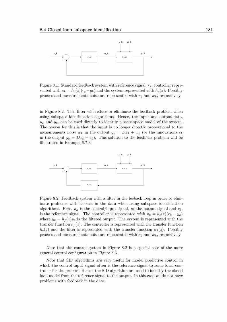
8.4 Closed loop subspace identification 181
h_p(z) h_c(z)
r_k u_k y_k
-
v_k w_k
Figure 8.1: Standard feedback system with reference signal, rk, controller repre-sented with uk = hc(z)(rk−yk) and the system represented with hp(z). Possiblyprocess and measurements noise are represented with vk and wk, respectively.
in Figure 8.2. This filter will reduce or eliminate the feedback problem whenusing subspace identification algorithms. Hence, the input and output data,uk and yk, can be used directly to identify a state space model of the system.The reason for this is that the input is no longer directly proportional to themeasurements noise wk in the output yk = Dxk + wk (or the innovations ek
in the output yk = Dxk + ek). This solution to the feedback problem will beillustrated in Example 8.7.3.
h_p(z) h_c(z)
r_k u_k y_k
-
v_k w_k
h_f(z)
Figure 8.2: Feedback system with a filter in the feeback loop in order to elim-inate problems with feeback in the data when using subspace identificationalgorithms. Here, uk is the control/input signal, yk the output signal and rk,is the reference signal. The controller is represented with uk = hc(z)(rk − yk)where yk = hf (z)yk is the filtered output. The system is represented with thetransfer function hp(z). The controller is represented with the transfer functionhc(z) and the filter is represented with the transfer function hf (z). Possiblyprocess and measurements noise are represented with vk and wk, respectively.
Note that the control system in Figure 8.2 is a special case of the moregeneral control configuration in Figure 8.3.
Note that SID algorithms are very useful for model predictive control inwhich the control input signal often is the reference signal to some local con-troller for the process. Hence, the SID algorithm are used to identify the closedloop model from the reference signal to the output. In this case we do not haveproblems with feedback in the data.
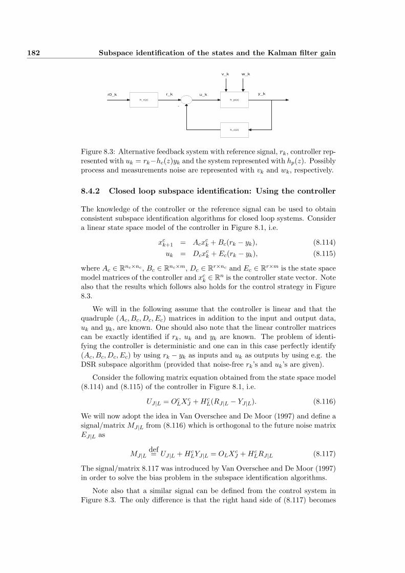
182 Subspace identification of the states and the Kalman filter gain
h_p(z)
h_c(z)
r_k h_r(z)
-
y_k u_k
v_k w_k
r_k r0_k
Figure 8.3: Alternative feedback system with reference signal, rk, controller rep-resented with uk = rk−hc(z)yk and the system represented with hp(z). Possiblyprocess and measurements noise are represented with vk and wk, respectively.
8.4.2 Closed loop subspace identification: Using the controller
The knowledge of the controller or the reference signal can be used to obtainconsistent subspace identification algorithms for closed loop systems. Considera linear state space model of the controller in Figure 8.1, i.e.
xck+1 = Acx
ck + Bc(rk − yk), (8.114)
uk = Dcxck + Ec(rk − yk), (8.115)
where Ac ∈ Rnc×nc , Bc ∈ Rnc×m, Dc ∈ Rr×nc and Ec ∈ Rr×m is the state spacemodel matrices of the controller and xc
k ∈ Rn is the controller state vector. Notealso that the results which follows also holds for the control strategy in Figure8.3.
We will in the following assume that the controller is linear and that thequadruple (Ac, Bc, Dc, Ec) matrices in addition to the input and output data,uk and yk, are known. One should also note that the linear controller matricescan be exactly identified if rk, uk and yk are known. The problem of identi-fying the controller is deterministic and one can in this case perfectly identify(Ac, Bc, Dc, Ec) by using rk − yk as inputs and uk as outputs by using e.g. theDSR subspace algorithm (provided that noise-free rk’s and uk’s are given).
Consider the following matrix equation obtained from the state space model(8.114) and (8.115) of the controller in Figure 8.1, i.e.
UJ |L = OcLXc
J + HcL(RJ |L − YJ |L). (8.116)
We will now adopt the idea in Van Overschee and De Moor (1997) and define asignal/matrix MJ |L from (8.116) which is orthogonal to the future noise matrixEJ |L as
MJ |Ldef= UJ |L + Hc
LYJ |L = OLXcJ + Hc
LRJ |L (8.117)
The signal/matrix 8.117 was introduced by Van Overschee and De Moor (1997)in order to solve the bias problem in the subspace identification algorithms.
Note also that a similar signal can be defined from the control system inFigure 8.3. The only difference is that the right hand side of (8.117) becomes
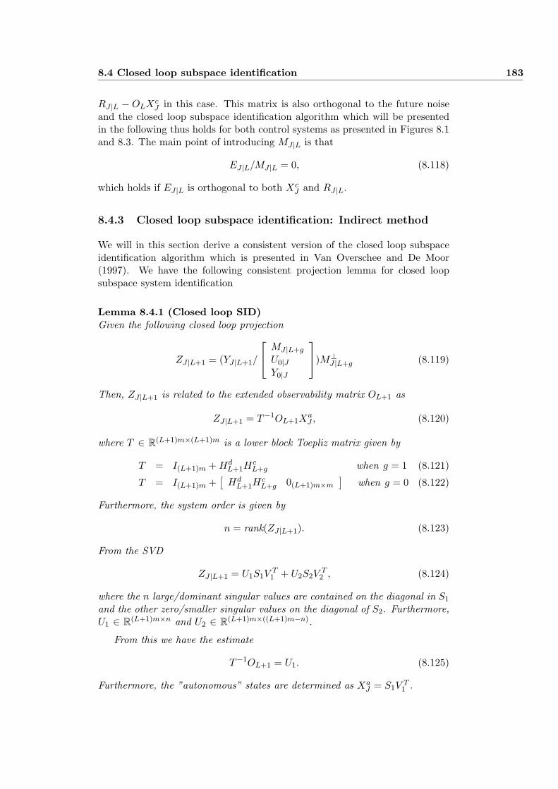
8.4 Closed loop subspace identification 183
RJ |L − OLXcJ in this case. This matrix is also orthogonal to the future noise
and the closed loop subspace identification algorithm which will be presentedin the following thus holds for both control systems as presented in Figures 8.1and 8.3. The main point of introducing MJ |L is that
EJ |L/MJ |L = 0, (8.118)
which holds if EJ |L is orthogonal to both XcJ and RJ |L.
8.4.3 Closed loop subspace identification: Indirect method
We will in this section derive a consistent version of the closed loop subspaceidentification algorithm which is presented in Van Overschee and De Moor(1997). We have the following consistent projection lemma for closed loopsubspace system identification
Lemma 8.4.1 (Closed loop SID)Given the following closed loop projection
ZJ |L+1 = (YJ |L+1/
MJ |L+g
U0|JY0|J
)M⊥
J |L+g (8.119)
Then, ZJ |L+1 is related to the extended observability matrix OL+1 as
ZJ |L+1 = T−1OL+1XaJ , (8.120)
where T ∈ R(L+1)m×(L+1)m is a lower block Toepliz matrix given by
T = I(L+1)m + HdL+1H
cL+g when g = 1 (8.121)
T = I(L+1)m +[
HdL+1H
cL+g 0(L+1)m×m
]when g = 0 (8.122)
Furthermore, the system order is given by
n = rank(ZJ |L+1). (8.123)
From the SVD
ZJ |L+1 = U1S1VT1 + U2S2V
T2 , (8.124)
where the n large/dominant singular values are contained on the diagonal in S1
and the other zero/smaller singular values on the diagonal of S2. Furthermore,U1 ∈ R(L+1)m×n and U2 ∈ R(L+1)m×((L+1)m−n).
From this we have the estimate
T−1OL+1 = U1. (8.125)
Furthermore, the ”autonomous” states are determined as XaJ = S1V
T1 .
184 Subspace identification of the states and the Kalman filter gain
Proof 8.13 A simple proof is given as follows. From (8.26) we have
YJ |L+1 = OL+1XJ + HdL+1UJ |L+g + Hs
L+1EJ |L+1. (8.126)
Adding HdL+1H
cL+gYJ |L+g on both sides of (8.126) and using the definition in
(8.117) gives
TYJ |L+1 = OL+1XJ + HdL+1MJ |L+g + Hs
L+1EJ |L+1. (8.127)
where T is as in (8.121) and (8.122). Since the matrix
MJ |L+g
U0|JY0|J
is uncor-
related (orthogonal) to the future noise matrix EJ |L+1 we have that
TZdJ |L+1 = OL+1X
dJ + Hd
L+1MJ |L+g (8.128)
where
ZdJ |L+1 =: YJ |L+1/
MJ |L+g
U0|JY0|J
, (8.129)
and
XdJ |L+1 =: XJ/
MJ |L+g
U0|JY0|J
, (8.130)
The lower triangular matrix T is non-singular if Im + EEc is non-singular.Hence,
ZdJ |L+1 = T−1OL+1X
dJ + T−1Hd
L+1MJ |L+g (8.131)
Post-multiplication of (8.131) with M⊥J |L+g proves (8.119) -(8.121).
Furthermore we have that
UT2 Zd
J |L+1 = UT2 T−1Hd
L+1MJ |L+g (8.132)
where U2 is the left singular vectors from the SVD of ZJ |L+1 which is re-lated to the ”zero/small” singular values. Equation (8.132) is obtained bypre-multiplying (8.131) with UT
2 and using that T−1OL+1 = U1 and UT2 U1 = 0.
Equation (8.132) is a linear equation of the elements in the lower blocktriangular Toepliz matrix T−1Hd
L+1. The solution to this problem is an im-portant step in the closed loop subspace algorithm and therefore needs furtherdiscussion. In order to do this we write (8.132) as
Y = UKMJ |L+g, (8.133)
8.4 Closed loop subspace identification 185
where
Y =: UT2 Zd
J |L+1 (8.134)
U =: UT2 (8.135)
K def= T−1HdL+1 ∈ R(L+1)m×(L+g)r (8.136)
The matrix K is a lower block triangular Toepliz matrix with m× r blocks Ki
∀ i = 1, . . . , L + 1. Hence, we can solve (8.132) (or equivalent (8.133) in a leastsquares optimal sense for the parameters in K. An algorithm for doing this ispresented in Van Overschee and De Moor (1996b) Appendix C.
The problem of solving (8.132) is very similar to the least squares problemin Section 8.3.4 for determining B and E for the open loop subspace problem.
Since HcL+g is known the matrix Hd
L+1 is simply obtained from K as (wheng = 1)
HdL+1 = K(I(L+1)r −Hc
L+gK)−1. (8.137)
Finally, the extended observability matrix of the system can be obtained as(when g = 1)
OL+1 = (I(L+1)m + HdL+1H
cL+g)U1. (8.138)
The system matrices A and D are then computed from OL+1. The systemmatrices B and E are computed from Hd
L+1 and OL.
The stochastic part of the system is determined very similar to the theoryin Section 8.3.3. The difference is that the projection matrix now is given by
ZsJ |L+1 = YJ |L+1 − YJ |L+1/
MJ |L+g
U0|JY0|J
= T−1Hs
L+1EJ |L+1 (8.139)
The projection matrices ZJ |L+1, ZdJ |L+1 and Zs
J |L+1 can effectively be computedby the LQ/QR decomposition.
The above ideas is among other details used to construct a MATLAB func-tion, dsr cl.m, for consistent closed loop subspace identification.
8.4.4 Closed loop subspace identification: Direct method
A drawback with the above algorithm is that T and HdL+1 have to be identified
before the extended observability matrix OL+1 and the system matrices A andD could be identified. We will in this section present a solution to the closedloop subspace identification problem which is more consistent with the DSRsubspace algorithm in which OL+1 and A and D is identified directly in a firststep. We have the following lemma
186 Subspace identification of the states and the Kalman filter gain
Lemma 8.4.2 (Direct closed loop SID)The extended observability matrix OL+1 is obtained from the following projection
ZJ |L+1 = ZdJ |L+1(MJ |L+g −Hc
L+1ZdJ |L+1)
⊥
= ZdJ |L+1(UJ |L+g + Hc
L+1ZsJ |L+1)
⊥ = OL+1XaJ (8.140)
where ZdJ |L+1 and Zs
J |L+1 are defined in (8.129) and (8.139), respectively.
Furthermore, B and E (or also HdL+1) can be obtained from
ZdJ |L+1 = OL+1X
dJ + Hd
L+1(MJ |L+g −HcL+1Z
dJ |L+1) (8.141)
or from (as in the standard DSR algorithm) the equation
ZdJ+1|L+1 − ALZJ |L = BL(MJ |L+g −Hc
L+1ZdJ |L+1) (8.142)
Proof 8.14 From (8.128) we have that
(I + HdL+1H
cL+g)Z
dJ |L+1 = OL+1X
dJ + Hd
L+1MJ |L+g. (8.143)
Rearranging (8.143) gives
ZdJ |L+1 = OL+1X
dJ + Hd
L+1(MJ |L+g −HcL+gZ
dJ |L+1) (8.144)
The closed loop subspace algorithm which is presented in this section is verysimilar to the open loop subspace identification algorithm which is presented inSection 8.3. The only difference is that the projection matrices are modified toincorporate the Markov parameters of the controller (the Toepliz matrix Hc
L+g.
8.5 A new subspace identification method for closedand open loop systems
It was presented in Di Ruscio (1995) and proved in Di Ruscio (2001) that thenoise innovation process could be identified directly from the data in a firststep. This approach is valid for both open and closed loop systems.
We will in the following consider a closed loop system in which it make senseto assume that E = 0. Putting g = 0 and letting J → ∞ in Equation ( 8.27)gives
YJ |1 = D[
CdJ Cs
J
] [U0|JY0|J
]+ FEJ |1. (8.145)
Hence, the innovations can simply be identified as (for g = 0)
ZsJ |1 = FEJ |1 = YJ |1 − YJ |1/
[U0|JY0|J
](8.146)
8.5 A new subspace identification method for closed and open loop systems 187
This result is also obtained directly from Lemma 3.9, and Di Ruscio (2001). Itis clear that the above approach is valid for both open and closed loop systemssince the past data, U0|J and Y0|J , is uncorrelated with the future noise EJ |1.
The innovations is known and the DSR algorithm is used directly with theinnovations as extra inputs in order to identify the ”deterministic” model
xk+1 = Axk +[
B K] [
uk
εk
], (8.147)
yk − εk = Dxk. (8.148)
We now simply solve a deterministic subspace identification problem in orderto obtain the system matrices A, B, K and D. Any efficient subspace method,e.g. the DSR method as presented earlier in this paper, can be used.
The DSR algorithm for closed loop systems is sketched simply as follows:
1. From the known input and output data uk and yk ∀ k = 0, 1, . . . , N − 1and a large past horizon, J , the future innovations matrix Zs
J |1 = FEJ |1 iscomputed from (8.146). The projection involved can be computed directlyfrom the definition or preferably from a QR decomposition.
2. The innovations sequence εk ∀ k = J, J+1, . . . , N−1 in the Kalman filteris given directly from the corresponding data in Zs
J |1. From the knowninnovations sequence we form the Hankel matrix EJ |L+1.
3. Define the known input and output data sequence uk and yk ∀ k = J, J +1, . . . , N − 1 and form the matrices UJ |L and YJ |L+1.
4. The data from step 2 and 3 and a specified future horizon, L, are usedto identify the state space model by an efficient subspace identificationmethod. As a rule of thumb, chose L small such that 1 ≤ n ≤ Lm. Thetheory in Sections 3.2 and 3.4 can be used directly by zeroing out thematrices U0|J and Y0|J from the projections.
Hence, we simply obtain the model matrices in the Kalman filter from theprojection equations
ZJ |L+1 = YJ |L+1
[UJ |LEJ |L+1
]⊥≈ OL+1X
aJ (8.149)
which gives OL+1, A and D and
YJ+1|L = ALYJ |L +[
BL CL
] [UJ |LEJ |L+1
](8.150)
gives B and K according to the theory in Section 3.4. This algorithm is imple-mented in the DSR e MATLAB function in the D-SR Toolbox for MATLAB.
188 Subspace identification of the states and the Kalman filter gain
8.6 Further remarks
8.6.1 Choice of algorithm parameters
There are two parameters in the algorithm, i.e., L and J . L is interpreted asthe identification-horizon used to predict the number of states. J is interpretedas the horizon (into the past) used to define instruments from the data whichare used to remove noise. The system order, n, which is specified or identified,is bounded by the user-specified parameter L, i.e. so that, 1 ≤ n ≤ mL wherem is the number of outputs. Hence, Lm singular values are computed by thealgorithm and the user may chose the system order, n, by inspection of the, n,non-zero singular values.
A rule of thumb is that L should be chosen as small as possible if the inputsare poorly exciting. The minimum identification-horizon, Lmin, so that the pair(D, A) is observable and rank(OLmin) = n is bounded by, d n
me ≤ Lmin ≤ n−rank(D)+1, where d·e is the ceiling function, i.e., rounding towards plus infinity.If the outputs are independent, then, we suggest to use Lmin = n−m+1 whenn ≥ m and Lmin = 1 when n = m. If the inputs are rich, e.g. white, thenthis point is not critical. In practice, it is suggested that model validationon independent data is taken into consideration when choosing the ”optimal”settings for L.
The past horizon, J , may for combined deterministic and stochastic systemsand for pure stochastic systems usually be chosen as J = L + 1 or J = L. Notethat the estimates of C and the Kalman filter gain matrix K = CF−1 usuallybecomes better when J increases. For pure deterministic systems we may choseJ = 1. The instruments Y0|J and U0|J can also be removed from the projections,i.e., and putting J = 0, in this case.
The theory in this paper is the basis for the D-SR Toolbox for MATLABwhich are available upon request. The toolbox consists of MATLAB functionsfor subspace system identification of both open and closed loop systems.
8.6.2 Choice of input signal
The subspace identification methods tends to be more sensitive to the inputsignal compared to e.g, the Prediction Error Method (PEM). This means thatthere may exist colored input signals which gives subspace estimates which areas optimal (efficient and consistent) as the PEM estimates. On the other sidethere may exist colored input signals where the subspace methods gives poorerresults compared to the PEM. An optimal experiment for the subspace methodsis in general not a white noise input, but rather a colored input signal where thefrequency spectrum is optimized to excite the parameters in the system as wellas possible. Our experience is also that an input signal which are minimizingthe condition number of the Hankal matrix U0|J or UJ |L+g, is usually not anoptimal input signal.
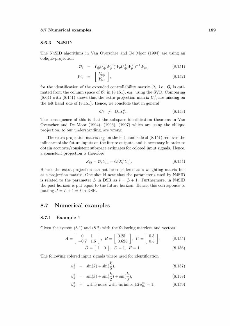
8.7 Numerical examples 189
8.6.3 N4SID
The N4SID algorithms in Van Overschee and De Moor (1994) are using anoblique-projection
Oi = Yi|iU⊥i|iW
Tp (WpU
⊥i|iW
Tp )−1Wp, (8.151)
Wp =[
U0|iY0|i
], (8.152)
for the identification of the extended controllability matrix Oi, i.e., Oi is esti-mated from the column space of Oi in (8.151), e.g. using the SVD. Comparing(8.64) with (8.151) shows that the extra projection matrix U⊥
i|i are missing onthe left hand side of (8.151). Hence, we conclude that in general
Oi 6= OiXai . (8.153)
The consequence of this is that the subspace identification theorems in VanOverschee and De Moor (1994), (1996), (1997) which are using the obliqueprojection, to our understanding, are wrong.
The extra projection matrix U⊥i|i on the left hand side of (8.151) removes the
influence of the future inputs on the future outputs, and is necessary in order toobtain accurate/consistent subspace estimates for colored input signals. Hence,a consistent projection is therefore
Zi|i = OiU⊥i|i = OiX
ai U⊥
i|i. (8.154)
Hence, the extra projection can not be considered as a weighting matrix butas a projection matrix. One should note that the parameter i used by N4SIDis related to the parameter L in DSR as i = L + 1. Furthermore, in N4SIDthe past horizon is put equal to the future horizon. Hence, this corresponds toputting J = L + 1 = i in DSR.
8.7 Numerical examples
8.7.1 Example 1
Given the system (8.1) and (8.2) with the following matrices and vectors
A =[
0 1−0.7 1.5
], B =
[0.250.625
], C =
[0.50.5
], (8.155)
D =[
1 0], E = 1, F = 1. (8.156)
The following colored input signals where used for identification
u1k = sin(k) + sin(
k
2), (8.157)
u2k = sin(k) + sin(
k
2) + sin(
k
3), (8.158)
u3k = withe noise with variance E(u2
k) = 1. (8.159)
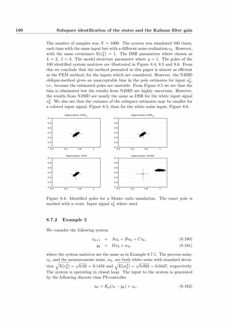
190 Subspace identification of the states and the Kalman filter gain
The number of samples was N = 1000. The system was simulated 100 times,each time with the same input but with a different noise realization ek. However,with the same covariance E(e2
k) = 1. The DSR parameters where chosen asL = 2, J = 3. The model structure parameter where g = 1. The poles of the100 identified system matrices are illustrated in Figure 8.4, 8.5 and 8.6. Fromthis we conclude that the method presented in this paper is almost as efficientas the PEM method, for the inputs which are considered. However, the N4SIDoblique-method gives an unacceptable bias in the pole estimates for input u1
k,i.e., because the estimated poles are unstable. From Figure 8.5 we see that thebias is eliminated but the results from N4SID are highly uncertain. However,the results from N4SID are nearly the same as DSR for the white input signalu3
k. We also see that the variance of the subspace estimates may be smaller fora colored input signal, Figure 8.5, than for the white noise input, Figure 8.6.
0.4 0.6 0.8 10.1
0.2
0.3
0.4
0.5
0.6
0.7
Eigenvalues: DSRc1
0.4 0.6 0.8 10.1
0.2
0.3
0.4
0.5
0.6
0.7
Eigenvalues: DSRc2
0.4 0.6 0.8 10.1
0.2
0.3
0.4
0.5
0.6
0.7Eigenvalues: PEM
0.4 0.6 0.8 10.1
0.2
0.3
0.4
0.5
0.6
0.7Eigenvalues: N4SID
Figure 8.4: Identified poles for a Monte carlo simulation. The exact pole ismarked with a cross. Input signal u1
k where used.
8.7.2 Example 2
We consider the following system
xk+1 = Axk + Buk + Cvk, (8.160)yk = Dxk + wk, (8.161)
where the system matrices are the same as in Example 8.7.1. The process noise,vk, and the measurements noise, wk, are both white noise with standard devia-tion
√E(v2
k) =√
0.02 = 0.1458 and√
E(w2k) =
√0.002 = 0.0447, respectively.
The system is operating in closed loop. The input to the system is generatedby the following discrete time PI-controller
uk = Kp(rk − yk) + zk, (8.162)
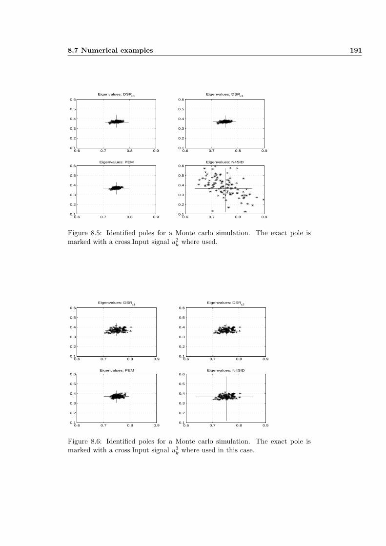
8.7 Numerical examples 191
0.6 0.7 0.8 0.90.1
0.2
0.3
0.4
0.5
0.6
Eigenvalues: DSRc1
0.6 0.7 0.8 0.90.1
0.2
0.3
0.4
0.5
0.6
Eigenvalues: DSRc2
0.6 0.7 0.8 0.90.1
0.2
0.3
0.4
0.5
0.6Eigenvalues: PEM
0.6 0.7 0.8 0.90.1
0.2
0.3
0.4
0.5
0.6Eigenvalues: N4SID
Figure 8.5: Identified poles for a Monte carlo simulation. The exact pole ismarked with a cross.Input signal u2
k where used.
0.6 0.7 0.8 0.90.1
0.2
0.3
0.4
0.5
0.6
Eigenvalues: DSRc1
0.6 0.7 0.8 0.90.1
0.2
0.3
0.4
0.5
0.6
Eigenvalues: DSRc2
0.6 0.7 0.8 0.90.1
0.2
0.3
0.4
0.5
0.6Eigenvalues: PEM
0.6 0.7 0.8 0.90.1
0.2
0.3
0.4
0.5
0.6Eigenvalues: N4SID
Figure 8.6: Identified poles for a Monte carlo simulation. The exact pole ismarked with a cross.Input signal u3
k where used in this case.
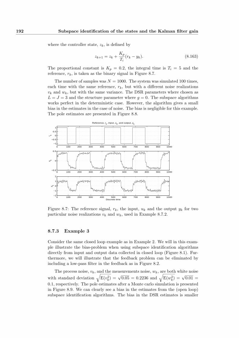
192 Subspace identification of the states and the Kalman filter gain
where the controller state, zk, is defined by
zk+1 = zk +Kp
Ti(rk − yk). (8.163)
The proportional constant is Kp = 0.2, the integral time is Ti = 5 and thereference, rk, is taken as the binary signal in Figure 8.7.
The number of samples was N = 1000. The system was simulated 100 times,each time with the same reference, rk, but with a different noise realizationsvk and wk, but with the same variance. The DSR parameters where chosen asL = J = 3 and the structure parameter where g = 0. The subspace algorithmsworks perfect in the deterministic case. However, the algorithm gives a smallbias in the estimates in the case of noise. The bias is negligible for this example.The pole estimates are presented in Figure 8.8.
0 100 200 300 400 500 600 700 800 900 1000
−1
−0.5
0
0.5
1
Reference, rk, input, u
k, and output, y
k
r k
0 100 200 300 400 500 600 700 800 900 1000−0.5
0
0.5
u k
0 100 200 300 400 500 600 700 800 900 1000−2
−1
0
1
2
Discrete time
y k
Figure 8.7: The reference signal, rk, the input, uk and the output yk for twoparticular noise realizations vk and wk, used in Example 8.7.2.
8.7.3 Example 3
Consider the same closed loop example as in Example 2. We will in this exam-ple illustrate the bias-problem when using subspace identification algorithmsdirectly from input and output data collected in closed loop (Figure 8.1). Fur-thermore, we will illustrate that the feedback problem can be eliminated byincluding a low-pass filter in the feedback as in Figure 8.2.
The process noise, vk, and the measurements noise, wk, are both white noisewith standard deviation
√E(v2
k) =√
0.05 = 0.2236 and√
E(w2k) =
√0.01 =
0.1, respectively. The pole estimates after a Monte carlo simulation is presentedin Figure 8.9. We can clearly see a bias in the estimates from the (open loop)subspace identification algorithms. The bias in the DSR estimates is smaller
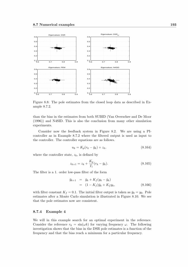
8.7 Numerical examples 193
0.6 0.7 0.8 0.90.1
0.2
0.3
0.4
0.5
0.6Eigenvalues: DSR
0.6 0.7 0.8 0.90.1
0.2
0.3
0.4
0.5
0.6
Eigenvalues: DSRc2
0.6 0.7 0.8 0.90.1
0.2
0.3
0.4
0.5
0.6Eigenvalues: PEM
0.6 0.7 0.8 0.90.1
0.2
0.3
0.4
0.5
0.6Eigenvalues: N4SID
Figure 8.8: The pole estimates from the closed loop data as described in Ex-ample 8.7.2.
than the bias in the estimates from both SUBID (Van Overschee and De Moor(1996)) and N4SID. This is also the conclusion from many other simulationexperiments.
Consider now the feedback system in Figure 8.2. We are using a PI-controller as in Example 8.7.2 where the filtered output is used as input tothe controller. The controller equations are as follows.
uk = Kp(rk − yk) + zk, (8.164)
where the controller state, zk, is defined by
zk+1 = zk +Kp
Ti(rk − yk). (8.165)
The filter is a 1. order low-pass filter of the form
yk+1 = yk + Kf (yk − yk)= (1−Kf )yk + Kfyk, (8.166)
with filter constant Kf = 0.1. The initial filter output is taken as y0 = y0. Poleestimates after a Monte Carlo simulation is illustrated in Figure 8.10. We seethat the pole estimates now are consistent.
8.7.4 Example 4
We will in this example search for an optimal experiment in the reference.Consider the reference rk = sin(ωk) for varying frequency ω. The followinginvestigation shows that the bias in the DSR pole estimates is a function of thefrequency and that the bias reach a minimum for a particular frequency.
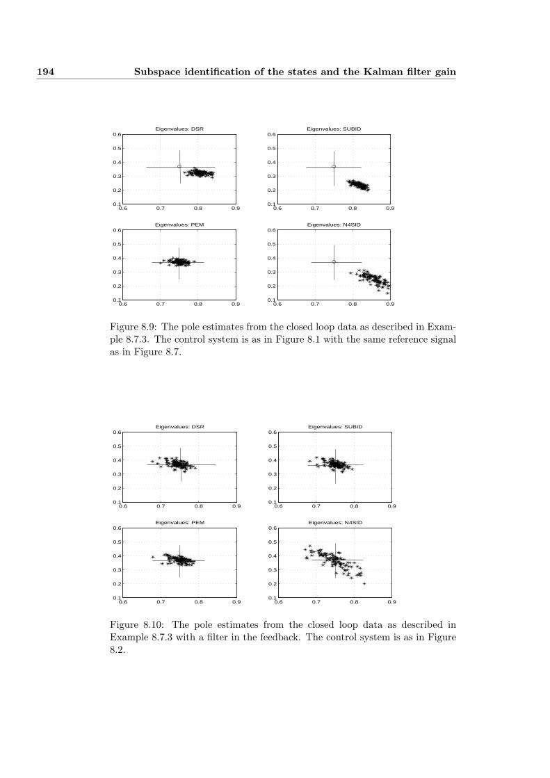
194 Subspace identification of the states and the Kalman filter gain
0.6 0.7 0.8 0.90.1
0.2
0.3
0.4
0.5
0.6Eigenvalues: DSR
0.6 0.7 0.8 0.90.1
0.2
0.3
0.4
0.5
0.6Eigenvalues: SUBID
0.6 0.7 0.8 0.90.1
0.2
0.3
0.4
0.5
0.6Eigenvalues: PEM
0.6 0.7 0.8 0.90.1
0.2
0.3
0.4
0.5
0.6Eigenvalues: N4SID
Figure 8.9: The pole estimates from the closed loop data as described in Exam-ple 8.7.3. The control system is as in Figure 8.1 with the same reference signalas in Figure 8.7.
0.6 0.7 0.8 0.90.1
0.2
0.3
0.4
0.5
0.6Eigenvalues: DSR
0.6 0.7 0.8 0.90.1
0.2
0.3
0.4
0.5
0.6Eigenvalues: SUBID
0.6 0.7 0.8 0.90.1
0.2
0.3
0.4
0.5
0.6Eigenvalues: PEM
0.6 0.7 0.8 0.90.1
0.2
0.3
0.4
0.5
0.6Eigenvalues: N4SID
Figure 8.10: The pole estimates from the closed loop data as described inExample 8.7.3 with a filter in the feedback. The control system is as in Figure8.2.
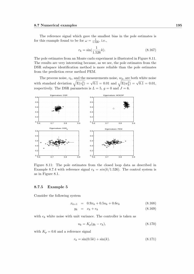
8.7 Numerical examples 195
The reference signal which gave the smallest bias in the pole estimates isfor this example found to be for ω = 1
1.526 , i.e.,
rk = sin(1
1.526k). (8.167)
The pole estimates from an Monte carlo experiment is illustrated in Figure 8.11.The results are very interesting because, as we see, the pole estimates from theDSR subspace identification method is more reliable than the pole estimatesfrom the prediction error method PEM.
The process noise, vk, and the measurements noise, wk, are both white noisewith standard deviation
√E(v2
k) =√
0.1 = 0.01 and√
E(w2k) =
√0.1 = 0.01,
respectively. The DSR parameters is L = 5, g = 0 and J = 6.
0.6 0.7 0.8 0.90.1
0.2
0.3
0.4
0.5
0.6Eigenvalues: DSR
0.6 0.7 0.8 0.90.1
0.2
0.3
0.4
0.5
0.6Eigenvalues: MOESP
0.6 0.7 0.8 0.90.1
0.2
0.3
0.4
0.5
0.6
Eigenvalues: DSRcl
0.6 0.7 0.8 0.90.1
0.2
0.3
0.4
0.5
0.6Eigenvalues: PEM
Figure 8.11: The pole estimates from the closed loop data as described inExample 8.7.4 with reference signal rk = sin(k/1.526). The control system isas in Figure 8.1.
8.7.5 Example 5
Consider the following system
xk+1 = 0.9xk + 0.5uk + 0.6ek (8.168)yk = xk + ek (8.169)
with ek white noise with unit variance. The controller is taken as
uk = Kp(yk − rk), (8.170)
with Kp = 0.6 and a reference signal
rk = sin(0.5k) + sin(k). (8.171)
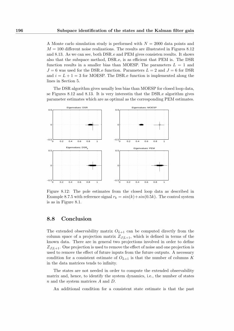
196 Subspace identification of the states and the Kalman filter gain
A Monte carlo simulation study is performed with N = 2000 data points andM = 100 different noise realizations. The results are illustrated in Figures 8.12and 8.13. As we can see, both DSR e and PEM gives consisten results. It showsalso that the subspace method, DSR e, is as efficient that PEM is. The DSRfunction results in a smaller bias than MOESP. The parameters L = 1 andJ = 6 was used for the DSR e function. Parameters L = 2 and J = 6 for DSRand i = L + 1 = 3 for MOESP. The DSR e function is implemented along thelines in Section 5.
The DSR algorithm gives usually less bias than MOESP for closed loop data,se Figures 8.12 and 8.13. It is very interestin that the DSR e algorithm givesparameter estimates which are as optimal as the corresponding PEM estimates.
0 0.2 0.4 0.6 0.8 1−0.5
0
0.5Eigenvalues: DSR
0 0.2 0.4 0.6 0.8 1−0.5
0
0.5Eigenvalues: MOESP
0 0.2 0.4 0.6 0.8 1−0.5
0
0.5
Eigenvalues: DSRe
0 0.2 0.4 0.6 0.8 1−0.5
0
0.5Eigenvalues: PEM
Figure 8.12: The pole estimates from the closed loop data as described inExample 8.7.5 with reference signal rk = sin(k)+sin(0.5k). The control systemis as in Figure 8.1.
8.8 Conclusion
The extended observability matrix OL+1 can be computed directly from thecolumn space of a projection matrix ZJ |L+1, which is defined in terms of theknown data. There are in general two projections involved in order to defineZJ |L+1. One projection is used to remove the effect of noise and one projection isused to remove the effect of future inputs from the future outputs. A necessarycondition for a consistent estimate of OL+1 is that the number of columns Kin the data matrices tends to infinity.
The states are not needed in order to compute the extended observabilitymatrix and, hence, to identify the system dynamics, i.e., the number of statesn and the system matrices A and D.
An additional condition for a consistent state estimate is that the past
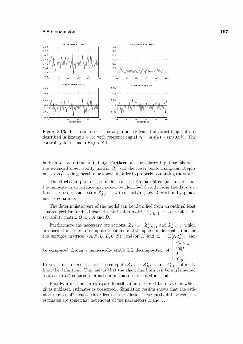
8.8 Conclusion 197
0 20 40 60 80 1000.4
0.42
0.44
0.46
0.48
0.5
0.52
0.54B parameter DSR
0 20 40 60 80 100−0.1
0
0.1
0.2
0.3
0.4
0.5
0.6B parameter MOESP
0 20 40 60 80 1000.4
0.45
0.5
0.55
0.6
0.65
B parameter DSRe
Realizations0 20 40 60 80 100
0.4
0.45
0.5
0.55
0.6
0.65B parameter PEM
Realizations
Figure 8.13: The estimates of the B parameter from the closed loop data asdescribed in Example 8.7.5 with reference signal rk = sin(k) + sin(0.5k). Thecontrol system is as in Figure 8.1.
horizon J has to tend to infinity. Furthermore, for colored input signals boththe extended observability matrix OL and the lower block triangular Toeplizmatrix Hd
L has in general to be known in order to properly computing the states.
The stochastic part of the model, i.e., the Kalman filter gain matrix andthe innovations covariance matrix can be identified directly from the data, i.e.from the projection matrix Zs
J |L+1, without solving any Riccati or Lyapunovmatrix equations.
The deterministic part of the model can be identified from an optimal leastsquares problem defined from the projection matrix Zd
J |L+1, the extended ob-servability matrix OL+1, A and D.
Furthermore the necessary projections, ZJ |L+1, ZdJ |L+1 and Zs
J |L+1, whichare needed in order to compute a complete state space model realization forthe sixtuple matrices (A,B, D, E, C, F ) (and/or K and ∆ = E(εkε
Tk )), can
be computed throug a numerically stable LQ decomposition of
UJ |L+g
U0|JY0|JYJ |L+1
.
However, it is in general faster to compute ZJ |L+1, ZdJ |L+1 and Zs
J |L+1 directlyfrom the definitions. This means that the algorithm both can be implementedas an correlation based method and a square root based method.
Finally, a method for subspace identification of closed loop systems whichgives unbiased estimates is presented. Simulation results shows that the esti-mates are as efficient as those from the prediction error method, however, theestimates are somewhat dependent of the parameters L and J .
198 Subspace identification of the states and the Kalman filter gain
References
Di Ruscio, D. (2003). Subspace system identification of the Kalman filter.Modeling, Identification and Control. Vol24, No.3, pp. 125-157.
Di Ruscio, D. (2001). Subspace system identification of the Kalman filter gain.The European Control Conference, ECC2001, Porto, Portogal 2001.
Di Ruscio, D. (1997). A method for identification of combined deterministicstochastic systems. In: Applications of Computer Aided Time Series Mod-eling, Lecture Notes in Statistics 119, Eds. M. Aoki and A. M. Havenner,Springer Verlag, ISBN 0-387-94751-5.
Di Ruscio, D. (1997b). On Subspace Identification of the Extended Observ-ability Matrix. In the proceedings of the 36th Conference on Decision andControl 1997, San Diego, California, December 6-14.
Di Ruscio, D. (1996). Combined Deterministic and Stochastic System Identifi-cation and Realization: DSR-a subspace approach based on observations.Modeling, Identification and Control, vol. 17, no.3.
Di Ruscio, D. (1995). A method for identification of combined deterministicstochastic systems: robust implementation. The Third European ControlConference ECC95, September 5-8, Rome, Italy.
D-SR Toolbox for MATLAB. Copyright D. Di Ruscio. Available upon request,[email protected].
Larimore, W. E. (1990). Canonical Variate Analysis in Identification, Filteringand Adaptive Control. Proc. of the 29th Conference on Decision andControl, Honolulu, Hawaii, December 1990, pp. 596-604.
Kung, S. Y. (1978). A new identification and Model Reduction Algorithm viaSingular Value Decomposition. Conf. on Circuits, Systems and Comput-ers, Pacific Grove, CA, November 1978, pp. 705-714.
Van Overschee, P. and B. De Moor (1994). N4SID: Subspace Algorithms forthe Identification of Combined Deterministic Stochastic Systems. Auto-matica, vol. 30, No. 1, pp.75-94.
Van Overschee, P. and B. De Moor (1996). Subspace Identification for LinearSystems: theory-implementation-applications. Kluwer Academic Publish-ers.
Van Overschee, P. and B. De Moor (1996b). Closed loop subspace system iden-tification. Internal report. Katholieke Universiteit Leuven. DepartmentElektrotechniek. ESAT-SISTA/TR 1996-521.
Van Overschee, P. and B. De Moor (1997). Closed loop subspace systemidentification. In the proceedings of the 36th Conference on Decision andControl 1997, San Diego, California, December 6-14.

8.8 Conclusion 199
Verhagen, M. (1994). Identification of the deterministic part of MIMO statespace models given on innovations form from input output data. Auto-matica, vol. 30, No. 1, pp. 61-74.
Viberg, M. (1995). Subspace-Based Methods for the Identification of LinearTime-invariant Systems. Automatica, vol. 31, No. 12, pp. 1835-1851.

200 Subspace identification of the states and the Kalman filter gain
Chapter 9
Effect of Scaling and how toTreat Trends
9.1 The data
We will consider some system input and output data vectors
uk ∀ k = 1, · · · , Nyk ∀ k = 1, · · · , N
}Known system input and output data (9.1)
We will assume that the data can be modeled by a linear discrete timecombined deterministic and stochastic state space model. The data does notnecessarily have to be stationary. Constant trends or drifts is represented withnon-stationary series which can be modeled by a state space model with poleson the unit circle.
9.2 The data matrices
From the known input and output series (9.1) we define the data matrices asfollows
Known data matrix of output variables︷ ︸︸ ︷
Y =
yT1
yT2
...yT
N
∈ RN×m (9.2)
Known data matrix of input variables︷ ︸︸ ︷
U =
uT1
uT2
...uT
N
∈ RN×r (9.3)
202 Effect of Scaling and how to Treat Trends
9.3 Scaling the data matrices
Consider the scaled system input and output data
usk = Suuk ∀ k = 1, · · · , N
ysk = Syyk ∀ k = 1, · · · , N
}Known scaled input and output data. (9.4)
The scaled input and output data vectors can be organized into data-matricessimilarly as in (9.2) and (9.3). However, the matrices which are identified shouldbe “unscaled” in order to satisfy the underlying (unscaled) system. A procedurefor incorporating scaling matrices is presented in Algorithm 9.3.1.
Algorithm 9.3.1 (Modeling procedure with scaled data matrices)Step 1, scaling the data: From the data matrices, Equations (9.2) and (9.3),and some scaling matrices Sy and Su, we define the scaled data matrices
Y s = Y STy , (9.5)
U s = USTu . (9.6)
Step 2, identification: The problem of identifying a complete linear (usu-ally) dynamic model for the process can be solved by the DSR function (seeD-SR Toolbox for Matlab).
[A, Bs, Ds, Es, C, F s
]= DSR(Y s, U s, L), (9.7)
where L is a positive scalar.
Step 3, unscaling: The matrices
B = BsSu, D = S−1y Ds, E = S−1
y EsSu, F = S−1y F s, (9.8)
satisfy the SSM
xk+1 = Axk + Buk + Cesk, (9.9)
yk = Dxk + Euk + Fesk, (9.10)
where esk has unit covariance.
Step 4, Kalman filter: The innovations form of the model (Kalman filter)is given by
xk+1 = Axk + Buk + Kek, (9.11)yk = Dxk + Euk + ek, (9.12)
where K is the Kalman filter gain
K = CF−1. (9.13)
ek is the innovations with covariance matrix
E(ekeTk ) = FF T . (9.14)
4
Remark 9.1 One particular and common choice is to chose the scaling matri-ces Sy and Su so that each column (variable) in the data-matrices Y s and U s
has unit variance.
9.3 Scaling the data matrices 203
9.3.1 Proof of Step 3 in Algorithm 9.3.1
The sixfold matrices (A,Bs, C, Ds, Es, F s) are the scaled state space modelmatrices (in the state space model)
xk+1 = Axk + Bsusk + Ces
k, (9.15)ys
k = Dsxk + Esusk + F ses
k, (9.16)
where esk has unit covariance matrix, i.e., E(es
k(esk)
T ) = I. Substituting for ysk
and usk given by (9.4) we get
xk+1 = Axk +
B︷ ︸︸ ︷BsSu uk + Ces
k, (9.17)Syyk = Dsxk + EsSuuk + F ses
k. (9.18)
Assume that Sy is non-singular. Post multiply Equation (9.18) with S−1y we
get
yk = S−1y Ds
︸ ︷︷ ︸D
xk + S−1y EsSu︸ ︷︷ ︸
E
uk + S−1y F s
︸ ︷︷ ︸F
esk. (9.19)
Hence, we have
B = BsSu, D = S−1y Ds, E = S−1
y EsSu, F = S−1y F s. (9.20)
To write the model on innovations (Kalman filter) form we define (from thenoise term in Equation (9.19))
ek = S−1y F ses
k, (9.21)
where ek is the innovations with covariance matrix
E(ekeTk ) = S−1
y F s(F s)T (S−1y )T , (9.22)
because esk has unit covariance.
From Equation (9.21) we get
esk = (F s)−1Syek. (9.23)
Substituting for esk into equations (9.17) and (9.19) we get the innovations form
of the state space model
xk+1 = Axk + Buk +
K︷ ︸︸ ︷C(F s)−1Sy ek, (9.24)
yk = Dxk + Euk + ek, (9.25)
where the Kalman filter gain matrix K is overbraced. QED.
204 Effect of Scaling and how to Treat Trends
9.3.2 Numerical Examples
Example 9.1 (Monte Carlo simulation)Monte Carlo simulations of a MIMO system with two inputs (r = 2), twooutputs (m = 2) and three states (n = 3) was worked out in order to analyzethe effect of scaling the input and output data on the pole estimates. Note that,in this case, the minimal identification parameter L is Lmin = n−m+1 = 2 ifthe two output variables are independent. The output variables are independentin this example. The DSR parameter L was varyed from L = 2 to L = 6.
Conclusions drawn when scaled data was used:
• Scaling the inputs gave no effect upon the pole estimates. The statisticaldistribution of the pole estimates was unchanged.
• In general, output scaling of the type Y s = Y STy where Sy is a gen-
eral non-singular matrix, can destroy the statistical distribution of thepole estimates. However, this was only observed when L > Lmin whereLmin = 2. The statistical distribution seams to depend on the chice ofscaling. A question is, does there exist an optimal scaling matrix Sy whichshould be used when L > Lmin.
• Irrespective of scaling the output variables, the statistical distribution ofthe pole estimates was unchanged when the minimal parameter L = Lmin =2 was used.
• Irrespective of choice of L, the statistical distribution of the pole estimateswas unchanged when each column (variable) in Y was equally scaled, i.e.,for scaling matrices Sy = diag(s, · · · , s) where s is a non-zero scalar.
Conclusions drawn when trended data was used:
• The system order increased by one when dtrended data (i.e., data withconstant trends removed) was used. A unit pole is included in the systemin order to handle the trends.
9.4 How to handle trends and drifts
Time series usually has a trend. Such trends can be nonzero constants or meanvalues, low frequency noise or drifts. The trends are often aprori unknown andtime varying. Assume that the output yk from a system can be separated intothree parts. One deterministic part yd
k which is driven from the known inputsuk, one stochastic part ys
k driven from unknown inputs or disturbances and onepart y0
k which represents the trend.
yk = ydk + ys
k + y0k. (9.26)
9.4 How to handle trends and drifts 205
In some applications we do not distinguish between the stochastic part ysk and
the trend y0k, i.e. we treat them simultaneously. The deterministic part, the
stochastic part and the trend may have common as well as separate and differentdynamics.
Constant non-zero trends and drifts can be described by a state space modelwhich has a pole on the unit circle. Low-frequency noise can be characterizedby a state space model which has a pole close to the unit circle. Such trendscan approximately be described by a random walk (drift)
x0k+1 = x0
k + vk, (9.27)y0
k = x0k, (9.28)
where vk is assumed to be a white and Gaussian distributed disturbance. Thisis a non-stationary process because the system has a pole on the unit circle.Trends can often be described by non-stationary processes which has a pole onthe unit circle.
Assume that the trend is purely time invariant (constant) and equal to y0,e.g., y0 can be the sample mean of the series yk. The trend can then be describedby a 1st order state space model with a pole equal to one (integrator)
x0k+1 = x0
k, x01 = y0, (9.29)
y0k = x0
k, (9.30)
where vk is assumed to be Gaussian distributed. The output y0k from this system
is purely exited by the initial values y0. The initial values which are identifiedare important because wrong initialization is not forgotten (because the systemis equal (or close) to an integrator).
It is not necessary to remove trends from the data when using DSR. Nonzeroconstant trends or drifts are usually identified and represented with low fre-quency dynamics, i.e. poles close to the unit circle.
One simple strategy is to first remove some constant trend from the dataand then identify the state space model matrices with initial values as follows,
[A, B, D, E, C, F ,x0
]= DSR(Y, U, L),
where Y and U are the data matrices adjusted for constant trends.
The constant trends which are removed can be the sample mean, the valuesof the series at time zero k = 1 or the mean of the first, say, j samples of theseries. A simple strategy for identifying constant trends , which are frequentlyused in practice, are given by
u0 =1j
j∑
k=1
uk, 1 ≤ j ≤ N, (9.31)
y0 =1j
j∑
k=1
yk, 1 ≤ j ≤ N. (9.32)
206 Effect of Scaling and how to Treat Trends
Nevertheless, even if this strategy is used, it is important to note that it can below-frequency dynamics in the estimated state space model. It is important tonote that this low-frequency dynamics often is incorporated in order to representtrends or drifts (which are not properly identified) in the output time series, itcan be decoupled from the dynamics from the known inputs uk to the outputsyk. In the following this is illustrated with some examples.
Example 9.2 (Using trended data)Assume a purely steady state deterministic system given by
yk = Euk. (9.33)
where E ∈ Rm×r is the gain matrix of the system.
Assume that a sequence of N input and output samples are given. We canthen define the data matrices Y and U . (Note the relationship Y = UET ).
Let us use a trended output data matrix for identification, i.e.,
Y s = Y − Y 0, (9.34)
where Y 0 is the trend (sample mean).
Using DSR for identification, i.e.,[
A, B, D, E, C, F ,x0
]= DSR(Y s, U, L),
we find the following 1st order state space model
xk+1 = xk, x1 = x0, (9.35)ys
k = Dxk + Euk. (9.36)
The estimated system has a unit pole. The reason for the unit pole is to handlethe trend. This means that both the trend Dxk = y0 as well as the gain matrixE are identified. We have that ys
k −Dxk = yk.
Example 9.3 (Non-stationary process)Consider the system
yk = euk + ysk, (9.37)
The output yk from this system consists of two parts. One purely steady statedeterministic part euk where e = −1 and one stochastic trend ys
k.
The trend is a drift which is described by
xk+1 = xk + vk, (9.38)ys
k = xk + wk, (9.39)
where vk and wk is serially uncorrelated and Gaussian distributed with unitvariance. The system (9.38) is a so called “random walk” which has a pole onthe unit circle (a = 1). The process is therefore not stationary.
9.5 Trends and low frequency dynamics in the data 207
The input to the system is exactly known and described by the random walk
zk+1 = zk + µk, (9.40)uk = zk, (9.41)
where µk is Gaussian distributed with unit variance and serially uncorrelatedwith vk and wk.
A Monte Carlo simulation of the system was done. I.e., the system (9.37)-(9.39) was simulated M = 500 times, each time with new realizations for vk andwk but with the same input (9.41). The number of samples for each simulationwas N = 5000,
500 different 1st order state space models was estimated from the 500 se-quences of input and output data (uk, yk, ∀, k = 1, · · · , N).
The innovations model for the system is
xk+1 = axk + buk + cek, (9.42)yk = xk + euk + ek. (9.43)
where a = 1, b = 0 and e = −1. The “exact” Kalman filter gain matrix isc = 0.6180 and the variance of the innovations is E(e2
k) = 2.6180.
The mean and standard deviation of the 500 estimated set of parameters(for the innovations model) are given by
a = 0.9994± 0.0007, b = 0.0000± 0.0009, e = −1.0017± 0.0220,c = 0.6188± 0.0132, E(e2
k) = 2.6083± 0.0532.
}(9.44)
Note that the estimated model parameters was scaled so that d = 1. The pa-rameters was estimated by DSR with identification horizon L = 2 (used foridentification of the number of states) and past horizon J = 5 (used to defineinstruments).
For comparison a purely steady state algorithm was used. The mean andstandard deviation of the gain estimates from PLS was
e = −0.9891± 1.2538}
PLS with raw data (9.45)
e = −0.9758± 0.7409}
PLS with centered data (9.46)
The mean of the parameters is not to bad. However, the standard deviation islarge which makes the estimates unreal-able.
9.5 Trends and low frequency dynamics in the data
There are basically two different approaches to deal with trends and slow dis-turbances in the data:
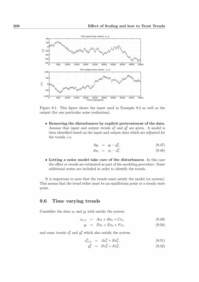
208 Effect of Scaling and how to Treat Trends
0 500 1000 1500 2000 2500 3000 3500 4000 4500 5000−80
−60
−40
−20
0
20
40The input time series: u_k
u_k
0 500 1000 1500 2000 2500 3000 3500 4000 4500 5000−100
−50
0
50
100The output time series : y_k
Time [samples]
y_k
Figure 9.1: This figure shows the input used in Example 9.3 as well as theoutput (for one particular noise realization).
• Removing the disturbances by explicit pretreatment of the data.Assume that input and output trends u0
t and y0t are given. A model is
then identified based on the input and output data which are adjusted forthe trends, i.e.
dyt = yt − y0t , (9.47)
dut = ut − u0t . (9.48)
• Letting a noise model take care of the disturbances. In this casethe offset or trends are estimated as part of the modeling procedure. Someadditional states are included in order to identify the trends.
It is important to note that the trends must satisfy the model (or system).This means that the trend either must be an equilibrium point or a steady statepoint.
9.6 Time varying trends
Considder the data ut and yt wich satisfy the system
xt+1 = Axt + But + Cet, (9.49)yt = Dxt + Eut + Fet, (9.50)
and some trends u0t and y0
t which also satisfy the system
x0t+1 = Ax0
t + Bu0t , (9.51)
y0t = Dx0
t + Eu0t . (9.52)
9.7 Constant trends 209
In this case the deviations du0t = ut − u0
t and dy0t = yt − y0
t will also satisfy thesystem, i.e.
xt+1 − x0t+1 = A(xt − x0
t ) + B(ut − u0t ) + Cet, (9.53)
yt − y0t = A(xt − x0
t ) + E(ut − u0t ) + Fet, (9.54)
This means that the adjusted data dut and dyt satisfy the system model (A,B, D,E, CF, F )with states dxt = xt − x0
t .
9.7 Constant trends
Assume that the data are adjusted for some constant trends or working pointsu0 and y0. It is important to note that such trends must satisfy the steadystate (static) relationship of the system, i.e.
y0 = Hdu0 (9.55)
where Hd is the steady state deterministic gain matrix
Hd = D(I −A)−1 + E. (9.56)
The data adjusted for the constant trends
dyt = yt − y0, (9.57)dut = ut − u0, (9.58)
will also satisfy the system given by (A,B, D, E,C, F ). This can relatively easybe prooved in the frequency domain.
An approximation of these steady state trends wich are commonly used inpractice are the sample mean
y0 =1N
N∑
t=1
yt, (9.59)
u0 =1N
N∑
t=1
ut. (9.60)
Another strategy which are found from practical experiences to work well inmost cases is to identify the working point from the mean of the first fewsamples.

210 Effect of Scaling and how to Treat Trends
Chapter 10
Validation
10.1 Model validation and fit
In order to measure the quality of a model we have to define some criteria.Consider a multivariable system with m output variables stacked on each otherin the output vector yt and r input variables stacked on each other in the inputvector ut.
We will in the following assume that we have a set of input and output timeseries (or observations)
ut
yt
}∀ t = 1, · · · , N (10.1)
for model validation.
10.1.1 Criteria based on the simulated error
Assume that a deterministic model (i.e. some model matrices (A, B,D, E)and a set of input and output validation data, as defined in (10.1), are given.Simulation will then give us the simulated outputs
xdt+1 = Axd
t + But (10.2)
ydt = Dxd
t + Eut (10.3)
where the initial state vector xd1 is known/specified 1
The difference between each actual output and each simulated output canbe measured by the following criteria.
Definition 10.1 (Mean Square Error (MSE))Define [yo]t as (validation) output channel/number o and [yd
o ]t for the simulated1Note that the super-script d stands for deterministic and that the actual state vector xt
can be splitted into two parts, i.e., deterministic and stochastic states, satisfying xt = xdt +xs
t .
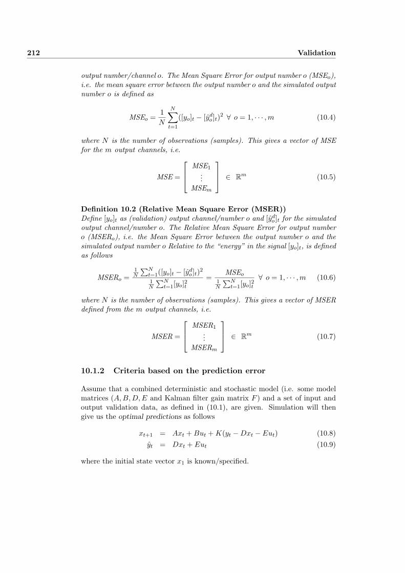
212 Validation
output number/channel o. The Mean Square Error for output number o (MSEo),i.e. the mean square error between the output number o and the simulated outputnumber o is defined as
MSEo =1N
N∑
t=1
([yo]t − [ydo ]t)2 ∀ o = 1, · · · ,m (10.4)
where N is the number of observations (samples). This gives a vector of MSEfor the m output channels, i.e.
MSE =
MSE1...
MSEm
∈ Rm (10.5)
Definition 10.2 (Relative Mean Square Error (MSER))Define [yo]t as (validation) output channel/number o and [yd
o ]t for the simulatedoutput channel/number o. The Relative Mean Square Error for output numbero (MSERo), i.e. the Mean Square Error between the output number o and thesimulated output number o Relative to the “energy” in the signal [yo]t, is definedas follows
MSERo =1N
∑Nt=1([yo]t − [yd
o ]t)2
1N
∑Nt=1[yo]2t
=MSEo
1N
∑Nt=1[yo]2t
∀ o = 1, · · · ,m (10.6)
where N is the number of observations (samples). This gives a vector of MSERdefined from the m output channels, i.e.
MSER =
MSER1...
MSERm
∈ Rm (10.7)
10.1.2 Criteria based on the prediction error
Assume that a combined deterministic and stochastic model (i.e. some modelmatrices (A,B, D, E and Kalman filter gain matrix F ) and a set of input andoutput validation data, as defined in (10.1), are given. Simulation will thengive us the optimal predictions as follows
xt+1 = Axt + But + K(yt −Dxt −Eut) (10.8)yt = Dxt + Eut (10.9)
where the initial state vector x1 is known/specified.
Chapter 11
Input experiment design
11.1 Experiment design for dynamic systems
Input experiment design for dynamic systems is discussed in , among others,Goodwin and Payne (1972) and Ljung (1989). We will in the following focus onBinary input Signals (BS) and Pseudo Random Binary input Signals (PRBS)and on some simple criteria for measuring the quality of different experimentdesign.
Assume that an input signal series
ut ∈ Rr ∀ 1 ≤ t ≤ N (11.1)
is given. From the input series (11.1) define the following input data matrixwith n + g block rows and K = N − n− k block columns.
Uk|n+gdef=
Known data matrix of input variables︷ ︸︸ ︷
uk uk+1 uk+2 · · · uk+K−1
uk+1 uk+2 uk+3 · · · uk+K...
......
. . ....
uk+n+g−2 uk+n+g−1 uk+n+g · · · uk+n+K+g−3
uk+n+g−1 uk+n+g uk+n+g+1 · · · uk+n+K+g−2
∈ R(n+g)r×K(11.2)
Definition 11.1 (Excitation condition)The input signal ut defined by (11.1) is defined to be exciting of order n if andonly if the matrix Uk|n+g is non-singular, i.e.
rank(Uk|n+g) = (n + g)r (11.3)
where g is a prescribed model structure parameter with values g = 0 if E = 0m×r
and g = 1 if E 6= 0m×r.
Definition 11.2 (Excitation condition)The input signal ut defined by (11.1) is defined to be exciting of order n if and
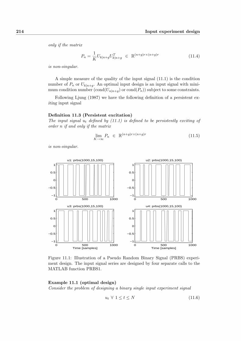
214 Input experiment design
only if the matrix
Pn =1K
Uk|n+gUTk|n+g ∈ R(n+g)r×(n+g)r (11.4)
is non-singular.
A simple measure of the quality of the input signal (11.1) is the conditionnumber of Pn or Uk|n+g. An optimal input design is an input signal with mini-mum condition number (cond(Un|n+g) or cond(Pn)) subject to some constraints.
Following Ljung (1987) we have the following definition of a persistent ex-iting input signal
Definition 11.3 (Persistent excitation)The input signal ut defined by (11.1) is defined to be persistently exciting oforder n if and only if the matrix
limK→∞
Pn ∈ R(n+g)r×(n+g)r (11.5)
is non-singular.
0 500 1000−1
−0.5
0
0.5
1
u1: prbs(1000,15,100)
0 500 1000−1
−0.5
0
0.5
1
u2: prbs(1000,15,100)
0 500 1000−1
−0.5
0
0.5
1
u3: prbs(1000,15,100)
Time [samples]0 500 1000
−1
−0.5
0
0.5
1
u4: prbs(1000,15,100)
Time [samples]
Figure 11.1: Illustration of a Pseudo Random Binary Signal (PRBS) experi-ment design. The input signal series are designed by four separate calls to theMATLAB function PRBS1.
Example 11.1 (optimal design)Consider the problem of designing a binary single input experiment signal
ut ∀ 1 ≤ t ≤ N (11.6)
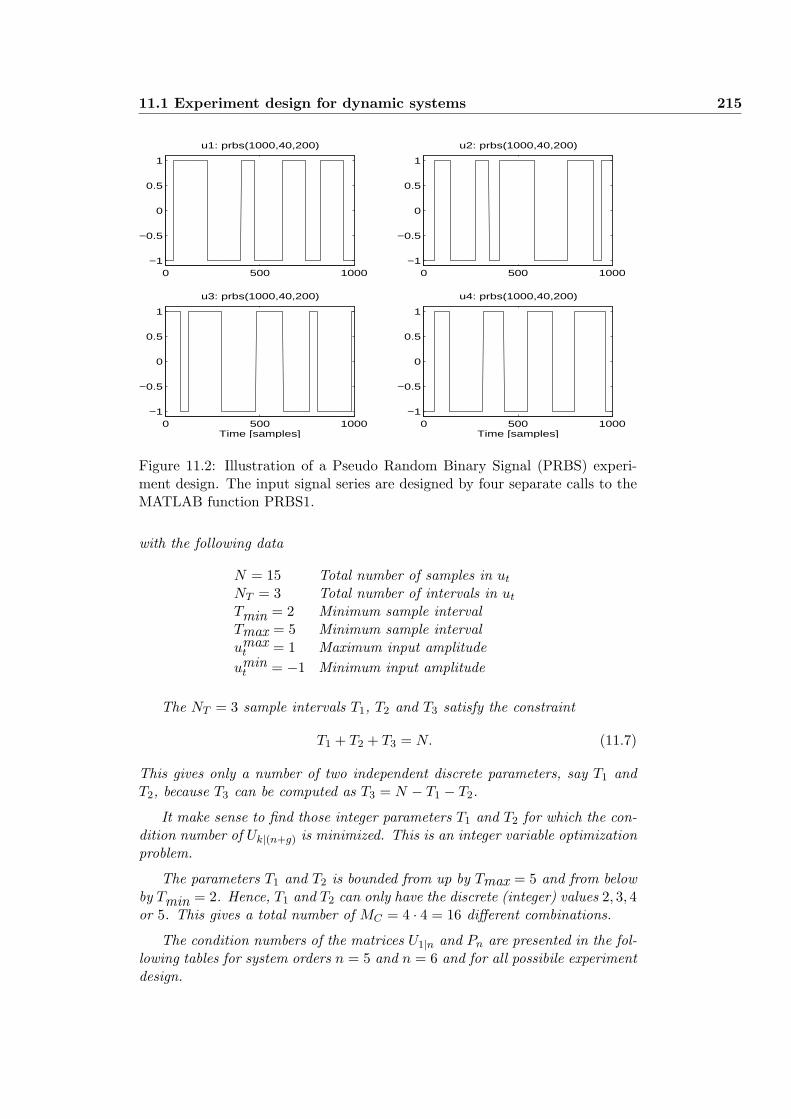
11.1 Experiment design for dynamic systems 215
0 500 1000−1
−0.5
0
0.5
1
u1: prbs(1000,40,200)
0 500 1000−1
−0.5
0
0.5
1
u2: prbs(1000,40,200)
0 500 1000−1
−0.5
0
0.5
1
u3: prbs(1000,40,200)
Time [samples]0 500 1000
−1
−0.5
0
0.5
1
u4: prbs(1000,40,200)
Time [samples]
Figure 11.2: Illustration of a Pseudo Random Binary Signal (PRBS) experi-ment design. The input signal series are designed by four separate calls to theMATLAB function PRBS1.
with the following data
N = 15 Total number of samples in ut
NT = 3 Total number of intervals in ut
Tmin = 2 Minimum sample intervalTmax = 5 Minimum sample intervalumax
t = 1 Maximum input amplitudeumin
t = −1 Minimum input amplitude
The NT = 3 sample intervals T1, T2 and T3 satisfy the constraint
T1 + T2 + T3 = N. (11.7)
This gives only a number of two independent discrete parameters, say T1 andT2, because T3 can be computed as T3 = N − T1 − T2.
It make sense to find those integer parameters T1 and T2 for which the con-dition number of Uk|(n+g) is minimized. This is an integer variable optimizationproblem.
The parameters T1 and T2 is bounded from up by Tmax = 5 and from belowby Tmin = 2. Hence, T1 and T2 can only have the discrete (integer) values 2, 3, 4or 5. This gives a total number of MC = 4 · 4 = 16 different combinations.
The condition numbers of the matrices U1|n and Pn are presented in the fol-lowing tables for system orders n = 5 and n = 6 and for all possibile experimentdesign.
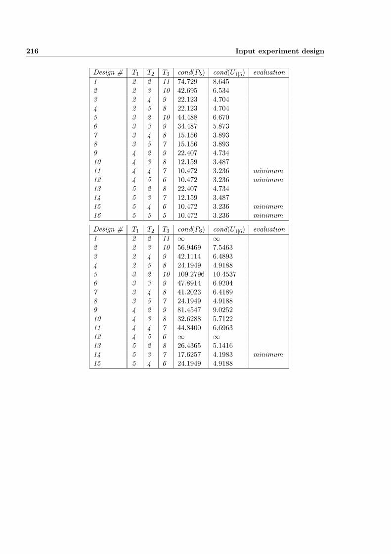
216 Input experiment design
Design # T1 T2 T3 cond(P5) cond(U1|5) evaluation1 2 2 11 74.729 8.6452 2 3 10 42.695 6.5343 2 4 9 22.123 4.7044 2 5 8 22.123 4.7045 3 2 10 44.488 6.6706 3 3 9 34.487 5.8737 3 4 8 15.156 3.8938 3 5 7 15.156 3.8939 4 2 9 22.407 4.73410 4 3 8 12.159 3.48711 4 4 7 10.472 3.236 minimum12 4 5 6 10.472 3.236 minimum13 5 2 8 22.407 4.73414 5 3 7 12.159 3.48715 5 4 6 10.472 3.236 minimum16 5 5 5 10.472 3.236 minimum
Design # T1 T2 T3 cond(P6) cond(U1|6) evaluation1 2 2 11 ∞ ∞2 2 3 10 56.9469 7.54633 2 4 9 42.1114 6.48934 2 5 8 24.1949 4.91885 3 2 10 109.2796 10.45376 3 3 9 47.8914 6.92047 3 4 8 41.2023 6.41898 3 5 7 24.1949 4.91889 4 2 9 81.4547 9.025210 4 3 8 32.6288 5.712211 4 4 7 44.8400 6.696312 4 5 6 ∞ ∞13 5 2 8 26.4365 5.141614 5 3 7 17.6257 4.1983 minimum15 5 4 6 24.1949 4.9188
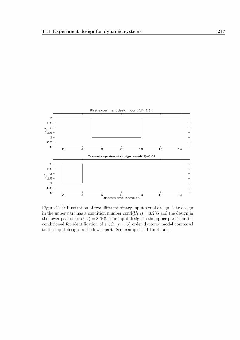
11.1 Experiment design for dynamic systems 217
2 4 6 8 10 12 140
0.5
1
1.5
2
2.5
3
u_k
Second experiment design: cond(U)=8.64
Discrete time [samples]
2 4 6 8 10 12 140
0.5
1
1.5
2
2.5
3
u_k
First experiment design: cond(U)=3.24
Figure 11.3: Illustration of two different binary input signal design. The designin the upper part has a condition number cond(U1|5) = 3.236 and the design inthe lower part cond(U1|5) = 8.645. The input design in the upper part is betterconditioned for identification of a 5th (n = 5) order dynamic model comparedto the input design in the lower part. See example 11.1 for details.

218 Input experiment design
Chapter 12
Special topics in systemidentification
12.1 Optimal predictions
For some time series we observe that the system dynamics are close to anintegrator and in particular for stochastic single output systems we may findthat the A parameter is close to one. In such cases we also often find that theoptimal Kalman filter prediction, yk, is approximately equal to the previousoutput yk−1. The reason for this is presented in the following proposition
Proposition 12.1 (Prediction equal to previous output)Consider a Kalman filter for a stochastic system xk+1 = Axk + vk and yk =Dxk + wk, i.e.,
xk+1 = Axk + K(yk − yk), (12.1)yk = Dxk. (12.2)
Assume that A = 1 (or A close to one) and DK = 1 (or DK close to one). Inthis case we have that the optimal prediction, yk, at present time k is equal tothe previous output yk−1, i.e.,
yk = yk−1. (12.3)
Proof 12.1From (12.1) and (12.2) with A = I we have that
∆xk = xk − xk−1 = K(yk−1 − yk−1), (12.4)yk = yk−1 + D∆xk (12.5)
This gives
yk = yk−1 + DK(yk−1 − yk−1), (12.6)
which gives Equation (12.3) when DK = 1. QED
220 Special topics in system identification
The Kalman filter is constructed to minimize the covariance of the estima-tion error, i.e. the parameters in the Kalman filter is found such that, e.g. thetrace of the matrix E((xk − xk)(xk − xk)T ) is minimized and usually also theprediction error criterion is minimized. Furthermore, given different models oneshould selected the best model from some validation criteria of the predictionerror criterion V = trace((E((yk − yk)(yk − yk)T )).
Chapter 13
On the Partial Least SquaresAlgorithm
13.1 Notation, basic- and system-definitions
Define yk ∈ Rm as a vector of output variables at observation number k. Theoutput variables are some times referred to as response variables. Similarly avector xk ∈ Rr of input variables is defined. It is assumed that the vector ofoutput variables yk are linearly related to the vector of input variables xk asfollows
yk = BT xk + ek, (13.1)
where ek is a vector of white noise with covariance matrix E(ekeTk ) and k is the
number of observation.
With N observations k = 1, · · · , N we define an output (or response) datamatrix Y ∈ RN×m and an input data matrix X ∈ RN×r as follows
Y =
yT1
...yT
N
, X =
xT1
...xT
N
. (13.2)
The data matrices Y and X are assumed to be known.
The linear relationship (13.1) can be written as the following linear matrixequation
Y = XB + E, (13.3)
where B is a matrix with regression coefficients. E ∈ RN×m is in general anunknown matrix of noise vectors, defined as follows
E =
eT1
...eTN
. (13.4)
222 On the Partial Least Squares Algorithm
The linear relationship between the output (response) and the input data (orregressors) is an important assumption and restriction for the PLS as well asany LS algorithm to work.
We will in this work analyze systems with multiple output variables in thedata matrix Y . This is often referred to as multivariable (or multivariate)systems.
If we only are interested in the matrix of regression coefficients B, then oneshould note that it (for steady state systems) usually is sufficient to consider oneoutput at a time and only investigate single output systems. This means thatthe multivariable LS problem can be solved from m single output LS problems,i.e., each column in B is estimated from a separated LS problem.
Note also that (instead of modeling one output variable at a time) equation(13.3) can be transformed to an equivalent model with one output in differ-ent ways. Two possibile models with one output, which are equivalent to themultivariable model (13.3) are preseted as follows
cs(Y ) = (Im ⊗X)cs(B) + cs(E), (13.5)cs(Y T ) = (X ⊗ Im)cs(BT ) + cs(ET ), (13.6)
where cs(·) is the column string operator and ⊗ is the Kronecker product. cs(Y )∈ RNm is a column vector constructed from Y by stacking each column in Yon another. We also have (Im ⊗X) ∈ RNm×rm and cs(B) ∈ Rrm.
Note that (13.6) can be constructed directly from (13.1) by first writing(13.1) as
yk = (xTk ⊗ Im)cs(BT ) + ek (13.7)
and then combine all N equations (k = 1, · · · , N) into a matrix equation of theform (13.3).
However, for the sake of completeness we will in general consider multivari-able (multiple output) systems of the form (13.3). One should also note thatthe PLS algorithm can be used to compute projections. An example is theproblem of computing the projection of the row space of Y T onto the row spaceof XT . In order to solve this problem we have to consider the general multipleoutput model (13.3).
13.2 Partial Least Squares
13.2.1 Interpretation of the Partial Least Squares algorithm
Define a vector t from the column space of X as t = Xw where w is a weightvector with constraint wT w = 1. The vector t is defined as the score vector forX. Similarly, a score vector u for Y is defined from the column space of Y asu = Y c where c is a weight vector with constraint cT c = 1.
13.2 Partial Least Squares 223
The PLS algorithm can be interpreted as the problem of computing weightvectors w and c which maximize the correlation between the score vector tand the score vector u. Hence, we have the problem of maximizing the functionf(w, c) = tT u with respect to w and c subject to the orthonormal constraints onw and c. We can formulate the key part in the PLS algorithm as the followingoptimization problem.
Problem 13.1 (PLS optimization problem) The key part in the PLS al-gorithm can be formulated as an optimization problem for each component.
Maximizef(w, c) = tT u,
with respect to w and c, wheret = Xw,u = Y c,
subject towT w = 1,cT c = 1.
(13.8)
4
The Lagrangian associated with this optimization problem is given by
L(w, c) = tT u + µ(1− wT w) + σ(1− cT c)= wT XT Y c + µ(1− wT w) + σ(1− cT c), (13.9)
where µ and σ are Lagrange multipliers associated with the constraints. Theoptimal solution is found by setting all possible derivatives of the Lagrangianto zero. We have
∂L∂c = Y T Xw − 2σc = 0, (13.10)∂L∂w = XT Y c− 2µw = 0, (13.11)∂L∂µ = 1− wT w = 0, (13.12)∂L∂σ = 1− cT c = 0. (13.13)
From Equations (13.10) and (13.11) we have
cT Y T Xw = 2σ, (13.14)wT XT Y c = 2µ. (13.15)
By transposing Equation (13.15) and comparing the result with Equation (13.14)shows that the Lagrange multipliers are equal, i.e., µ = σ.
From this it is clear that w and c are given by the following SVD problem
cT Y T Xw = s, (13.16)
or equivalently (by transposing (13.16))
wT XT Y c = s, (13.17)
224 On the Partial Least Squares Algorithm
where s = 2σ = 2µ is the singular value associated with XT Y or Y T X. Theweight vectors w and c can be taken as singular vectors of XT Y or Y T X.Furthermore, one should take w and c as the singular vectors associated withthe maximal singular value of XT Y (or Y T X). The reason for this is that theobjective
f(w, c) = tT u = wT XT Y c = s (13.18)
is maximized when s is the maximum singular value of XT Y . Note also thatif r > m then we should compute the economy size SVD of XT Y otherwise weshould work with Y T X. Further details of this SVD problem will be presentedand commented on in the next section.
From Equation (13.10) we have c = Y T Xw/(2σ). Substituting this intoEquation (13.11) gives an eigenvector problem for w. Similarly, from Equa-tion (13.11) we have w = XT Y c/(2µ). Substituting this into Equation (13.10)gives an eigenvector problem for c. Hence, we have the following eigenvec-tor/eigenvalue problems associated with the PLS algorithm
XT Y Y T Xw = λw, with wT w = 1, (13.19)Y T XXT Y c = λc, with cT c = 1, (13.20)
where the eigenvalue λ is related to the Lagrangian multipliers in (13.9) asλ = 4σµ. Note also that λ is related to the maximum singular value s of(13.16) or (13.17) as λ = s2.
Computing the orthonormal weight vectors w and c
From Section 13.2.1 it is clear that both weight vectors w and c can be computedas the left and right singular vectors of the matrix XT Y , respectively. We willin the following assume that r > m. Otherwise we should work with Y T X. Inthis case c is the left singular vector and w is the right singular vector associatedwith Y T X, respectively.
The key step in the PLS algorithm is the following singular value decompo-sition
XT Y = USVT , (13.21)
where U ∈ Rr×r is a matrix of left orthonormal singular vectors, V ∈ Rm×m is amatrix of right orthonormal singular vectors and S ∈ Rr×m is a diagonal matrixof singular values. Note that a reduced singular value decomposition can becomputed when r > m. In this case U ∈ Rr×m, S ∈ Rm×m and V ∈ Rm×m.
Define the maximum (largest) singular value of XT Y as s. Hence, s is equalto the upper left (first diagonal) element of the matrix S of singular values. Theweight vector w is given by the left singular vector associated with the largestsingular value. Similarly, the weight vector c is given by the right singular
13.2 Partial Least Squares 225
vector associated with the largest singular value. We have
w = U(:, 1), (13.22)c = V(:, 1), (13.23)s = S(1, 1). (13.24)
The weight vectors are orthonormal, i.e., they satisfy wT w = 1 and cT c = 1.The reason for this is that the columns of the SVD matrices U and V areorthonormal.
Equation (13.21) is central in the PLS algorithm. This can be shown asfollows. From the SVD in (13.21) it is clear that the eigenvector problems in(13.19) and (13.20) can be written as
XT Y Y T XU = USST , (13.25)Y T XXT Y V = VSTS, (13.26)
where SST ∈ Rr×r is a diagonal matrix with the eigenvalues of XT Y Y T Xalong the diagonal and STS ∈ Rm×m is a diagonal matrix with the eigenvaluesof Y T XXT Y along the diagonal.
After w and c are computed, the score vectors can be computed as follows
t = Xw, (13.27)u = Y c. (13.28)
The maximum correlation between the score vectors t and u is
maxw,c
f(w, c) = tT u = wT XT Y c = wTUSVT c = s, (13.29)
where s is the maximum singular value of XT Y , i.e. equal to the upper leftdiagonal element in S. This is the solution to the PLS optimization problem(13.8).
Remark 13.1 For one component, the maximum correlation between the tscore vector and the u score vector is equal to the maximum singular values of XT Y , i.e., tT u = s.
We have given an interpretation of the PLS algorithm for one component(also for the first component in the general PLS algorithm). The followingalgorithm illustrates the central part of the general PLS algorithm.
226 On the Partial Least Squares Algorithm
Algorithm 13.2.1 (Central part of the PLS algorithm)
X1 = Xfor i = 1, a Loop for all components 1 ≤ a ≤ r
XTi Y = USVT The Singular Value Decomposition
wi = U(:, 1) The weight vector for Xci = V(:, 1) The weight vector for Ysi = S(1, 1) The largest singular value of XT Yti = Xiwi The score vector for X
Xi+1 = (IN − titTi
tTi ti)Xi Rank one reduction of X
end
This results in a (score vector) matrix T ∈ RN×a with orthogonal columns,weight matrices C ∈ Rm×a and W ∈ Rr×a with orthonormal columns and adiagonal matrix S ∈ Ra×a of maximum singular values si of XT
i Y . The matricesare defined as follows
T =[
t1 · · · ta], C =
[c1 · · · ca
], W =
[w1 · · · wa
], (13.30)
S =
s1 · · · 0...
. . ....
0 sa
. (13.31)
4
The details in the algorithm will be discussed in the next sections.
Remark 13.2 For each new component a rank one reduced matrix Xi is usedin the SVD problem. Similarly it is common practice to use a rank one reducedmatrix Yi+1 = (IN − tit
Ti
tTi ti)Yi. In this case the SVD of the matrix XT
i Yi iscomputed at each iteration. However, rank one reduction of Y is not necessary.Further details will be discussed in the next Section 13.2.1.
Definition 13.1 Define a score matrix U of score vectors for Y computed froma rank one reduced matrix Yi as follows
U =[
u1 · · · ua
] ∈ RN×a, (13.32)
where the score vectors are given by
ui = Yici ∈ RN . (13.33)
4
13.2 Partial Least Squares 227
Remark 13.3 The maximum correlation matrix between the score vector ma-trix T and the score vector matrix U is equal to a lower triangular matrix L,i.e.,
T T U = L ∈ Ra×a, (13.34)
if the score matrix U is computed as in definition 13.1, i.e., from a rank onereduced (undeflated) matrix Yi.
The diagonal element number i of L is equal to the maximum singular valuesi of XT
i Y , i.e., lii = si, where lii is diagonal element number i in matrix L.This means that
tr(T T U) = tr(S), (13.35)
where S is defined by (13.31).
Proof of remark 13.3
The statement that L given by (13.34) is a lower triangular matrix can beproved as follows. The upper triangular elements of T T U = L are given by
li,i+1 = tTi ui+1 = tTi Yi+1ci+1 = tTi (I − titTi
tTi ti)Yici+1 = (tTi − tTi )Yici+1 = 0.(13.36)
QED.
Definition 13.2 Define a score matrix U for Y computed from an undeflatedY matrix as follows
U = Y C ∈ RN×a. (13.37)
Each score vector is defined as
ui = Y ci ∈ RN . (13.38)
4
Remark 13.4 The maximum correlation matrix between the score vector ma-trix T and the score matrix U is in general equal to a full matrix M definedas
T T U = M ∈ Ra×a, (13.39)
when matrix U is computed without Y deflation, i.e., as in Definition 13.2.
The diagonal element number i of M is equal to the maximum singular valuesi of XT
i Y , i.e., mii = si, where ii is diagonal element number i in matrix M .Hence
tr(T T U) = tr(S), (13.40)
where S is defined by (13.31).4
228 On the Partial Least Squares Algorithm
Gram-Schmidt orthogonalization
We have shown how the weight vectors w and c, and the score vectors t and uare computed (for one component) from the SVD of XT Y . See Section 13.2.1.
The next step in the PLS algorithm is a rank one reduction of X and Y .(However, one should note that rank one reduction of Y is not necessary). Thisstep is very central in the PLS algorithm and should therefore be discussed indetail. Define the following (rank one reduced) matrices from X, Y and thet-score vector.
Xi+1 = (IN − titTi
tTi ti)Xi, (13.41)
Yi+1 = (IN − titTi
tTi ti)Yi, (13.42)
where X1 = X and Y1 = Y . In the PLS algorithm, the weight vectors w and cand the score vectors t and u, for the next component, are computed based onthe rank one reduced matrices Xi+1 and Yi+1.
The score vector ti+1 (for the next component) is computed based on Xi+1
and Yi+1. This means that a new SVD of XTi+1Yi+1 is computed. The weight
vectors wi+1, ci+1 and the score vectors ti+1, ui+1 can be computed as shownin Section 13.2.1.
ti+1 is orthogonal to ti, i.e., tTi+1ti = 0. The rank one reduction, Equation(13.41) and (13.42), is similar to the Gram-Schmidt orthogonalization process.
The rank one reduction process can be written in terms of so called loadingvectors. The loading vector pi for Xi is defined as
pTi =
tTi Xi
tTi ti. (13.43)
The rank one reduction of X, Equation (13.41), can then be written as
Xi+1 = Xi − tipTi . (13.44)
Using that ti = Xiwi we have the following alternative to (13.43),
pTi =
wTi XT
i Xi
wTi XT
i Xiwi. (13.45)
The rank one reduction of Xi, Equation (13.41), can then be written as
Xi+1 = Xi(I − wipTi ). (13.46)
Equations (13.41), (13.44) and (13.46) can be used to formulate different PLSimplementations.
The loading vector ci for Y is defined as
cTi =
tTi Yi
tTi ti. (13.47)
13.2 Partial Least Squares 229
The rank one reduction of Yi, Equation (13.42), can then be written as
Yi+1 = Yi − ticTi . (13.48)
By using ti = Xiwi we can find alternative expressions for (13.47) and (13.48).
We will know show that the loading vector ci is related to the weight vectorci, i.e. related to the SVD of XT
i Yi. For convenience in the final PLS algorithmwe define a scaled weight (loading) vector ci for Yi as follows
ci =si
tTi tici, (13.49)
where si is the largest singular value of XTi Yi, i.e. the upper left (diagonal)
element in the matrix S of singular values.
Proof of equation (13.49)
For the sake of simplicity the subscript i is neglected in the following proof.The loading vector can be written as
c =Y T t
tT t=
Y T Xw
tT t, (13.50)
where we have used that t = Xw. Using that Y T X = VSTUT we have
c =Y T Xw
tT t=
1tT t
VSTUT w. (13.51)
The matrix U with left singular vectors for XT Y has orthonormal columns.The weight vector w is equal to the first column in U . Hence we have
UT w =
wT
uT2...
uTr
w =
10...0
. (13.52)
Using (13.52) we have that
STUT w =
s1 0 · · · 00 s2 · · · 0...
.... . .
...0 0 · · · sm
10...0
=
s1
0...0
=
s0...0
. (13.53)
By using (13.53) we have that
VSTUT w =[
c v2 · · · vm
]
s0...0
= sc. (13.54)
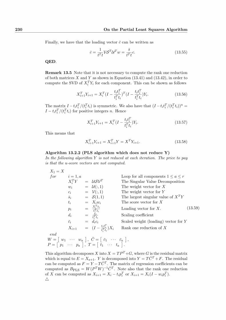
230 On the Partial Least Squares Algorithm
Finally, we have that the loading vector c can be written as
c =1
tT tVSTUT w =
s
tT tc. (13.55)
QED.
Remark 13.5 Note that it is not necessary to compute the rank one reductionof both matrices X and Y as shown in Equation (13.41) and (13.42), in order tocompute the SVD of XT
i Yi for each component. This can be shown as follows
XTi+1Yi+1 = XT
i (I − titTi
tTi ti)T (I − tit
Ti
tTi ti)Yi. (13.56)
The matrix I− titTi /(tTi ti) is symmetric. We also have that (I− tit
Ti /(tTi ti))n =
I − titTi /(tTi ti) for positive integers n. Hence
XTi+1Yi+1 = XT
i (I − titTi
tTi ti)Yi. (13.57)
This means that
XTi+1Yi+1 = XT
i+1Y = XT Yi+1. (13.58)
Algorithm 13.2.2 (PLS algorithm which does not reduce Y)In the following algorithm Y is not reduced at each iteration. The price to payis that the u-score vectors are not computed.
X1 = Xfor i = 1, a Loop for all components 1 ≤ a ≤ r
XTi Y = USVT The Singular Value Decomposition
wi = U(:, 1) The weight vector for Xci = V(:, 1) The weight vector for Ysi = S(1, 1) The largest singular value of XT Yti = Xiwi The score vector for X
pi = XTi ti
tTi tiLoading vector for X.
di = s1
tTi tiScaling coefficient
ci = dici Scaled weight (loading) vector for Y
Xi+1 = (I − titTi
tTi ti)Xi Rank one reduction of X
endW =
[w1 · · · wa
], C =
[c1 · · · ca
],
P =[
p1 · · · pa
], T =
[t1 · · · ta
].
(13.59)
This algorithm decomposes X into X = TP T +G, where G is the residual matrixwhich is equal to E = Xa+1. Y is decomposed into Y = TCT +F . The residualcan be computed as F = Y −TCT . The matrix of regression coefficients can becomputed as BPLS = W (P T W )−1CT . Note also that the rank one reductionof X can be computed as Xi+1 = Xi − tip
Ti or Xi+1 = Xi(I − wip
Ti ).
4
13.2 Partial Least Squares 231
Monte carlo simulation with PLS used on dynamical systems indicates thatadditional rank reduction of Y gives improved numerical precision. However,the effect of removing the rank reduction step on Y with respect to numericalprecision should be further investigated.
The partial regression
We will here study the rank one reduction of X and Y which is carried out foreach component in the PLS algorithm. This will in turn give us an expressionfor the PLS estimate of the regression coefficients.
Consider the rank one reduction (deflation) process of X and Y
Xi+1 = X − tpT , pT =tT X
tT t, (13.60)
and
Yi+1 = Y − tcT , cT = dcT , (13.61)
where we have defined the scalar d as
d =s
tT t. (13.62)
Using that t = Xw we have
Xi+1 = X(I − wpT ), (13.63)Yi+1 = Y −XwcT = Y −XwdcT . (13.64)
Comparing (13.64) with the assumed linear relationship Y = XB + E betweenX and Y , we have that the matrix of regression coefficients (for one componentonly) is given by
B1 = wcT = wdcT =s
tT twcT . (13.65)
The prediction of Y (for one component only) is then given by
Y1 = XB1 = XwcT . (13.66)
Hence, if the rank one reduction of Y is carried out at each step, it can beinterpreted as the residual
Yi+1 = Y − Y1. (13.67)
Example 13.1 (PLS with two components)Assume two components a = 2. The residual can be written as
Y3 = Y2 − t2cT2 = Y2 −X2w2c
T2 = Y2 −X2B2, (13.68)
232 On the Partial Least Squares Algorithm
where we have defined B2 = w2cT2 . Substituting for Y2 = Y −XB1 and X2 =
X(I − w1pT1 ) gives
Y3 = Y −XB1 −X(I − w1pT1 )B2 = Y −X(B1 + (I − w1p
T1 )B2). (13.69)
The PLS estimate of the matrix of regression coefficients B can be written as
BPLS = B1 + (I − w1pT1 )B2 = w1c
T1 + (I − w1p
T1 )w2c
T2 , (13.70)
where we have used that B1 = w1cT1 and B2 = w2c
T2 . This can be written in
matrix form as follows
BPLS =
W︷ ︸︸ ︷[w1 w2
](P T W )−1
︷ ︸︸ ︷[1 −pT
1 w2
0 1
] CT
︷ ︸︸ ︷[c1 c2
]T. (13.71)
It can in general be shown that BPLS = W (P T W )−1CT as indicated. Theloading matrix C can be written as
C =
C︷ ︸︸ ︷[c1 c2
]S︷ ︸︸ ︷[
s1
tT1 t10
0 s2
tT2 t2
]. (13.72)
The matrix of regression coefficients can then be written as
BPLS =
W︷ ︸︸ ︷[w1 w2
](P T W )−1
︷ ︸︸ ︷[1 −pT
1 w2
0 1
]S︷ ︸︸ ︷[
s1
tT1 t10
0 s2
tT2 t2
] CT
︷ ︸︸ ︷[c1 c2
]T. (13.73)
It can in general be shown that BPLS = W (P T W )−1SCT , where S is a diagonalmatrix with si/(tTi ti) on the diagonal.4
The PLS algorithm step for step
The following algorithm is presented in order to illustrate the computationsinvolved in the PLS algorithm. Refined PLS algorithms will be presented later.
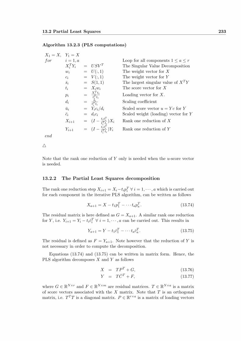
13.2 Partial Least Squares 233
Algorithm 13.2.3 (PLS computations)
X1 = X, Y1 = Xfor i = 1, a Loop for all components 1 ≤ a ≤ r
XTi Yi = USV T The Singular Value Decomposition
wi = U(:, 1) The weight vector for Xci = V (:, 1) The weight vector for Ysi = S(1, 1) The largest singular value of XT Yti = Xiwi The score vector for X
pi = XTi ti
tTi tiLoading vector for X.
di = si
tTi tiScaling coefficient
ui = Yici/di Scaled score vector u = Y c for Yci = dici Scaled weight (loading) vector for Y
Xi+1 = (I − titTi
tTi ti)Xi Rank one reduction of X
Yi+1 = (I − titTi
tTi ti)Yi Rank one reduction of Y
end
4
Note that the rank one reduction of Y only is needed when the u-score vectoris needed.
13.2.2 The Partial Least Squares decomposition
The rank one reduction step Xi+1 = Xi−tipTi ∀ i = 1, · · · , a which is carried out
for each component in the iterative PLS algorithm, can be written as follows
Xa+1 = X − t1pT1 − · · · tapT
a . (13.74)
The residual matrix is here defined as G = Xa+1. A similar rank one reductionfor Y , i.e. Yi+1 = Yi − tic
Ti ∀ i = 1, · · · , a can be carried out. This results in
Ya+1 = Y − t1cT1 − · · · tacT
a . (13.75)
The residual is defined as F = Ya+1. Note however that the reduction of Y isnot necessary in order to compute the decomposition.
Equations (13.74) and (13.75) can be written in matrix form. Hence, thePLS algorithm decomposes X and Y as follows
X = TP T + G, (13.76)Y = TCT + F, (13.77)
where G ∈ RN×r and F ∈ RN×m are residual matrices. T ∈ RN×a is a matrixof score vectors associated with the X matrix. Note that T is an orthogonalmatrix, i.e. T T T is a diagonal matrix. P ∈ Rr×a is a matrix of loading vectors
234 On the Partial Least Squares Algorithm
associated with X. C ∈ Rm×a is a matrix of scaled weight vectors (or loadingvectors) associated with Y .
The loading matrix (scaled weight matrix) C for Y can be decomposed into
C = CSΛ−1t = Y T TΛ−1
t , (13.78)
where C is a matrix with orthonormal columns ci, i.e., cTi ci = 1. See the
Appendix, Equation (13.185) for further details. ci can be taken from the rightsingular vectors of XT
i Y . S is a diagonal matrix with the maximum singularvalues si of XT
i Y on the diagonal. Λt is a diagonal matrix with tTi ti on thediagonal. Note that ti = Xiwi and that
Λt = T T T. (13.79)
The loading matrix P for X can then be decomposed into
P = PtΛ−1t , (13.80)
where Pt is the unscaled loading matrix with columns formed from the unscaledloading vectors, i.e.,
pt,i = XTi ti. (13.81)
We will in the next section use the above relations to formulate a PLS decom-position with an orthonormal score vector matrix for X.
By combining Equations (13.80) and (13.81) we find that the P loading ma-trix for X, in general can be expressed as P = XT T (T T T )−1. This expressionfor P can be proved by putting the gradient matrix of ‖ G ‖2
F with respect totr(P ) equal to zero. These results are presented in the following lemma.
Lemma 13.2.1 (PLS decomposition in terms of the T -score matrix)The P loading matrix for X and the C loading matrix for Y can in general beexpressed as
P = XT T (T T T )−1, (13.82)C = Y T T (T T T )−1, (13.83)
(13.84)
where we have assumed that T T T is non-singular.
The PLS decomposition, Equations (13.76) and (13.77), can in general beexpressed as
X = T (T T T )−1T T X + G, (13.85)Y = T (T T T )−1T T Y + F. (13.86)
The T ∈ RN×a score vector matrix for X can in general be expressed as
T = XW (P T W )−1 = XW (T T XW )−1(T T T ). (13.87)
4
13.2 Partial Least Squares 235
Orthonormal score vector matrix
In some applications, e.g. in subspace identification algorithms for dynamicsystems, orthonormal decompositions are prefered. The PLS decomposition,Equations (13.76) and (13.77), can be rewritten as
X = ToPTo + G, (13.88)
Y = ToCTo + F, (13.89)
where
To = TΛ− 1
2t , (13.90)
Po = PΛ12t = PtΛ
− 12
t , (13.91)
Co = CΛ12t = CSΛ
− 12
t . (13.92)
The scaled score vector To is orthonormal, i.e. T To To = Ia. Note that Λt = T T T
is a diagonal matrix.
Note also the following alternative description of the orthonormal PLS de-composition
X =
To︷ ︸︸ ︷TΛ
− 12
t
Po︷ ︸︸ ︷Λ− 1
2t P T
t +G, (13.93)
Y = TΛ− 1
2t Λ
− 12
t SCT
︸ ︷︷ ︸Co
+F. (13.94)
13.2.3 The Partial Least Squares regression and prediction
We will in this section discuss some alternative methods for computing the PLSestimate of the matrix of regression coefficients B.
From Equation (13.77) we have that the prediction of Y is given by
Y = TCT . (13.95)
Similarly, from Equation (13.76) we have that the prediction of X (or theinformation in X used for modeling Y ) is given by
X = TP T . (13.96)
The matrix of PLS regression coefficients is given by
B = W (P T W )−1CT . (13.97)
Note that only the weight matrix W , loading matrix C and the loading matrixP are needed in order to compute B. Hence, the score vector matrices T and Uare not explicitly needed. T is implicitly computed in order to define P and C.U need not to be computed in order to compute B. Note also that the matrix
236 On the Partial Least Squares Algorithm
P T W which have to be inverted is of size a × a. P T W is an upper triangularmatrix with ones on the diagonal. This should be utilized when computing Bfor numerical efficiency.
The matrix of PLS regression coefficients can equivalently be written as
B = W (P Tt W )−1SCT = W (T T XW )−1SCT , (13.98)
where P Tt W = T T XW is an upper triangular matrix with tTi ti on the diagonal.
Se also Lemma 13.2.1.
Proof of Equation (13.97)
The prediction of Y can be written as
Y = XB. (13.99)
Substituting for X = TP T and B given by (13.97) gives
Y = TP T W (P T W )−1CT = TCT , (13.100)
which is equivalent to Equation (13.95).QED.
The matrix of regression coefficients can be computed recursively during thePLS iterations. This is numerically preferable because we in this case do nothave to explicitly inverting the upper triangular matrix P T W . We have
B =a∑
i=1
(Ir − wi−1pTi−1)wic
Ti , w0 = 0, p0 = 0. (13.101)
This formula can be proved from the PLS updating expressions Yi+1 = Yi −Xiwic
Ti and Xi+1 = Xi(I − wip
Ti ). We also have the following alternative
expression
B =a∑
i=1
(Ir − wi−1pTi−1)wi
si
tTi ticTi , w0 = 0, p0 = 0. (13.102)
Remark 13.6 (Prediction) Note that the prediction of Y usually is com-puted as
Y = XB, (13.103)
when X is not used for computing B. Hence, Equation (13.103) is used forvalidation and prediction.
13.2 Partial Least Squares 237
13.2.4 Computing projections from the PLS decomposition
Consider the basic linear relationship
Y T = BT XT + ET . (13.104)
The projection of (the row space) of a matrix A onto (the row space) of a matrixB is defined as follows
A/B = ABT (BBT )†B, (13.105)
where (·)† denotes the Moore-Penrose pseudo inverse. We also define the pro-jection of the row space of A onto the orthogonal complement of the row spaceof B as
AB⊥ = A−ABT (BBT )†B. (13.106)
This implies that A is decomposed into two terms which are orthogonal to eachother, i.e.
A = A/B + AB⊥. (13.107)
Then we have the following projection of Y T onto XT .
Y T /XT = BT XT + ET /XT . (13.108)
The projection of ET onto XT is assumed to be zero. This is the case whenN → ∞ and the noise process ek is white and serially uncorrelated with xi.The projection can then be computed as
Y T /XT = BT XT . (13.109)
Substituting for the decomposition X = TP T and the estimate of the regressionmatrix B = W (P T W )−1CT into (13.109) gives
Y T /XT = C(P T W )−T W T PT T = CT T . (13.110)
Using the orthonormal PLS decomposition Y = ToCTo and X = ToP
To we have
the following alternative description
Y T /XT = CoPTo (PoP
To )−1
XT
︷ ︸︸ ︷PoT
To . (13.111)
where we have used (13.110). Comparing (13.111) with (13.108) shows that
BT = CoPTo (PoP
To )−1 and B = (PoP
To )−1PoC
To , (13.112)
when PoPTo ∈ Rr×r is non-singular.
Note also that the projection of Y T onto the orthogonal complement of XT
is equal to the residual GT from the PLS decomposition.
238 On the Partial Least Squares Algorithm
13.2.5 A semi standard PLS implementation
The version of the PLS algorithm which is presented in this section is denotedsemi standard because it is based on the SVD.
Algorithm 13.2.4 (Standard PLS implementation with SVD)
X1 = X, Y1 = Yfor i = 1, a Loop for all components 1 ≤ a ≤ r
XTi Yi = USV T The Singular Value Decomposition
wi = U(:, 1) The weight vector for Xti = Xiwi The score vector for X
ci = Y Ti ti
tTi tiScaled weight vector for Y
ui = Yici
cTi ci
Score vector for Y
pi = XTi ti
tTi tiLoading vector for X
Xi+1 = Xi − tipTi Updating of X, (rank one reduction of X)
Yi+1 = Yi − ticTi Updating of Y , (rank one reduction of Y )
end
The loading matrix P , the weight matrix W and the loading matrix C are thengiven by
P =[
p1 · · · pa
], W =
[w1 · · · wa
], C =
[c1 · · · ca
].(13.113)
The matrix of regression coefficients can then be computed as BPLS = W (P T W )−1CT .Note that P T W is upper triangular with ones on the diagonal.
The algorithm also computes the score vector matrices
T =[
t1 · · · ta], U =
[u1 · · · ua
]. (13.114)
4
13.2.6 The number of components a
The number of variables in X is r. The number of PLS components a (orfactors) is bounded from above by r. Hence,
1 ≤ a ≤ r.
The problem of choosing the number of components a is in general a trade ofbetween, on the one hand, “rank decision” based on the score matrices U andT or the largest singular values si of XT
i Yi, i = 1, · · · , r, and, on the other hand,model validation on independent data.
The PLS algorithm is constructed in order to maximize the linear relation-ship between the ui score for Yi and the ti score for Xi. Recall that the ui scorevector lies in the column space of Yi and that the ti score vector lies in the
13.3 Further interpretations of the PLS algorithm 239
column space of Xi. See Problem (13.1). In order to chose the effective numberof components a one can plot the score vector ui against the score vector ti forall i = 1, · · · , a and choose a from the plot where there is no linear relationshipbetween ua and ta.
Another strategy is simply to choose a as the number of “non zero” signifi-cant singular values si ∀ i = 1, · · · , r.
The problem of choosing a can of course be done recursively during thePLS iteration. One procedure is to plot ui against ti at each PLS iterationand by inspection decide if a new component should be incorporated. Anotherprocedure is to at each PLS iteration check if si is significant different fromzero.
We end this section by pointing out that it often make sense to be parsimo-nious when choosing the number of components.
13.3 Further interpretations of the PLS algorithm
13.3.1 General results
The results in this sections are general in the sense that it holds for all com-ponents a. However, we will restrict our results to 1 ≤ a ≤ r where r is thenumber of X variables.
Remark 13.7 We have the following general expression for the Squared Pre-diction Error (SPE) when the PLS algorithm is used
VN =‖ Y −XB ‖2F =‖ Y − TCT ‖2
F (13.115)
which can be expressed as
VN = tr(Y T Y )− 2tr(SΛ−1t T T Y C) + tr(CSΛ−1
t SCT ) (13.116)
by using that C = CS(T T T )−1. Furthermore, (13.116) can be evaluated as
VN (B) =‖ Y −XB ‖2F = tr(Y T Y )− tr(S2Λ−1
t )
= tr(Y T Y )−a∑
i=1
s2i
tTi ti, (13.117)
where we have assumed that Λt = T T T is non-singular. a is the number ofcomponents which usually is bounded as 1 ≤ a ≤ r. For each new componentwhich is incorporated, the variance in the output variables is reduced by thepositive term s2
i
tTi ti. It is assumed that tTi ti 6= 0.
4
Remark 13.8 Putting the gradient matrix of Equation (13.116) with respectto C equal to zero, gives the following general PLS condition
SCT = T T Y. (13.118)
240 On the Partial Least Squares Algorithm
This expression is to our knowledge new.
We have also derived a quite different and general expression for the SPEas follows.
Remark 13.9 Substituting Equation (13.118) into (13.116) shows that theSPE can be written as
VN = tr(Y T Y )− tr(Y T TΛ−1t T T Y ) = tr(Y T Y )− tr(Y T T0T
T0 Y ). (13.119)
The first term on the right hand side is the sum of variances for each output(response) variable (times N − 1). The second term is the sum of variances forthe predicted outputs (times N − 1), i.e.,
Y = XB = T\Y = TΛ−1t T T Y = ToT
To Y, (13.120)
where To is the orthogonal score matrix. Note that for finite N we have E(ykyTk ) ≈
1N−1 Y T Y and (N − 1)E(yky
Tk ) ≈ tr(Y T Y ).
The second term on the right hand side of (13.119) can be computed fromthe SVD of the matrix
Λ− 1
2t T T Y = T T
o Y = U SVT . (13.121)
Then,
VN = tr(Y T Y )−min(a,m)∑
i=1
s2i . (13.122)
Note the difference in the second term on the right hand side of Equations(13.117) and (13.122). The number of singular values s is a but the number ofsingular values si is min(a,m).4
13.3.2 Special case results
The results in this section holds in general only for one component, i.e., a = 1.
Remark 13.10 We have the following expression for the Squared PredictionError (SPE) when a = 1.
VN =‖ Y −XB1 ‖2F = tr(Y T Y )− s2
tT t, (13.123)
where T = t = Xw and s is the maximum singular value of XT Y . We haveassumed that tT t is non-singular.4

13.4 A covariance based PLS implementation 241
Remark 13.11 We have the following expression for the squared Frobeniusnorm of u− t
‖ u− t ‖2F = tr(Y T Y ) + tr(XT X)− 2tr(W T XT Y C), (13.124)
where t = XW and u = Y C. Hence, in the PLS algorithm the weight vectorsare computed as
minW,C
‖ t− u ‖2F = max
W,C(tT u). (13.125)
This gives an alternative interpretation of the basic PLS optimization Problem13.1.4
Remark 13.12 In methods to solve least squares problems it is often useful tohave some knowledge of the norm of the solution. An example is the Tikhonovregularized solution or the least squares solution with a quadratic inequality sideconstraint on the solution B. See Hansen (1992).
For PLS with one component (a = 1) we have
‖ B1 ‖F =s
tT t=‖ XT Y ‖F
wT XT Xw. (13.126)
Note that, in this case, the above also holds for the 2-norm of the solution, i.e.,by replacing ‖ · ‖F in (13.126) with ‖ · ‖2.
13.4 A covariance based PLS implementation
From the basic linear Equation (13.3) we have
XT Y = XT XB + XT E (13.127)
which is the normal equation for the LS problem. We will in the followingpresent a version of the PLS algorithm which works with XT Y and XT X ratherthan X and Y .
The weights w and c are computed from the SVD of XT Y . First, initialize(XT X)i = XT X and (XT Y )i = XT Y , then compute the weights wi and ci
from the SVD of (XT Y )i as follows,
(XT Y )i = USV T , wi = U(:, 1), ci = U(:, 1), si = S(1, 1). (13.128)
Compute the loading vector pi as
pi =(XT X)iwi
zi, where zi = wT
i (XT X)iwi. (13.129)
The loading vector ci can be computed as
ci =(XT Y )T
i wi
zi=
si
zici. (13.130)
242 On the Partial Least Squares Algorithm
Finally, the correlation matrix XT Y and the covariance matrix XT X are up-dated directly as
(XT X)i+1 = (I − wipTi )T (XT X)i(I − wip
Ti ), (13.131)
(XT Y )i+1 = (I − wipTi )T (XT Y )i. (13.132)
Equations (13.128) to (13.132) are computed for all i = 1, · · · , a components,where 1 ≤ a ≤ r. This procedure results in the matrices W , C and P . The ma-trix of regression coefficients can then be computed as BPLS = W (P T W )−1C.Remark that the product P T W is upper triangular with ones on the diagonal.This structure should be used for efficient computation of (P T W )−1.
The covariance based PLS implementation is very simple. It is very fastcompared to the traditional PLS when the number of observations N is verylarge compared to the number of input variables r and the number of outputvariables m.
The initialization of the covariance matrix XT X and the correlation ma-trix XT Y can be a problem due to rounding off errors when the number ofobservations N is large. The algorithm which is presented in the next sectionis numerically robust.
13.5 A square root PLS algorithm
Consider the QR decomposition of the concatenated matrix
[X Y
]=
[Q1 Q2
] [R11 R12
0 R22
]. (13.133)
From this we have that X = Q1R11 and Y = Q1R12 +Q2R22. Substituting intothe linear equation Y = XB + E gives the normal equation
R12 = R11B, (13.134)
where R11 ∈ Rr×r is upper triangular and R12 ∈ Rr×m.
A standard PLS algorithm can then be used to decompose R11 and R12 asfollows
R11 = TP T + G, (13.135)R12 = TCT + F (13.136)
and to compute the weighting matrix W . The PLS estimate of B is thenBPLS = W (P T W )−1CT .
The above algorithm is numerically robust in the sense that it avoid possiblyrounding off errors when computing XT Y . The reason for this is that the squareroot PLS algorithm instead works on XT Y = RT
11R12. However, the square rootPLS algorithm is not so fast as the covariance based PLS algorithm.
13.6 Undeflated PLS 243
13.6 Undeflated PLS
The PLS algorithm is iterative. At each iteration a rank one reduced (deflated)matrix Xi is computed. Usually a rank one reduction (deflation) of Y is alsocarried out. Deflation of Y is not necessary in order to compute the regressionmatrix B. The reason is that XT
i Yi = XTi Y . In the following an LS method
without deflation is presented. This method is denoted UDPLS. The resultsfrom UDPLS are in general different from the results from PLS.
Problem 13.2 (UDPLS optimization problem)
Maximizef(W,C) = tr(T T U),
with respect to W and C, whereT = XW,U = Y C,
subject toW T W = I,CT C = I.
The Lagrangian associated with this optimization problem is given by
L(w, c) = tr(W T XT Y C) + tr[ΓT (I −W T W )] + tr[ΣT (I − CT C)], (13.137)
where Γ and Σ are matrices with Lagrange multipliers associated with the con-straints. The optimal solution is found by setting all possible gradient matricesof the Lagrangian to zero. We have
∂L∂W
= (CT Y T X − 2ΓT W T )T = 0, ⇒ XT Y C = 2WΓ. (13.138)
∂L∂C
= (W T XT Y − 2ΣT CT )T = 0, ⇒ Y T XW = 2CΣ. (13.139)
These derivatives are restricted to symmetric matrices Γ and Σ.
For non-singular Σ we have C = 0.5Y T XWΣ−1, which gives
XT Y Y T XW = 4WΓΣ, (13.140)
Y T XXT Y C = 4CΣΓ. (13.141)
The key step is the following SVD
XT Y = USVT . (13.142)
This gives
XT Y Y T XU = USST , (13.143)Y T XXT Y V = VSTS. (13.144)
244 On the Partial Least Squares Algorithm
Chose W and C as
W = U , (13.145)C = V. (13.146)
Note that
T = XW, (13.147)T T U = W T XT Y C = S. (13.148)
The matrix of regression coefficients are given by
BUDPLS = W (T T T )−1SCT = U(UT XT XU)−1SV. (13.149)
where one should use only the a first components of T and U . The estimatecan also be written as
BUDPLS = U(UT XT XU)−1UT XT Y. (13.150)
Note that the above method is equivalent to the ordinary PLS algorithm whena = 1.
13.7 Total Least Squares and Truncated Total LeastSquares
Total Least Squares (TLS) and Truncated Total Least Squares (TTLS) aremethods for solving over-determined linear systems of equations. To be specific,TLS is a technique to solve models of the type Y = XB + E, where not onlythe left hand side Y is subject to errors but also X is subject to errors. Thismodel is known by statisticians as the errors in variables model. This model isalso known as a bi-linear model because Y is linear in both X and B but bothB and X is unknown, since X is subject to errors. Software for TLS and TTLSare presented in Hansen (1992).
13.7.1 Total Least Squares
Consider the Total Least Squares (TLS) problem
minZ,B
f(Z,B), (13.151)
where
f(Z,B) = ‖X − Z‖2F + ‖Y − ZB‖2
F , (13.152)
where ‖ · ‖F is the Frobenius norm. The solution to this optimization problemcan be found from the SVD of the compound (or concatenated) matrix [X Y ].We have
[X Y
]=
[U1 U2
] [S1 00 S2
] [V T
11 V T21
V T12 V22
], (13.153)
13.7 Total Least Squares and Truncated Total Least Squares 245
where U1 ∈ RN×r, U2 ∈ RN×m, S1 ∈ Rr×r, S2 ∈ Rm×m, V11 ∈ Rr×r, V12 ∈Rr×m, V21 ∈ Rm×r and V22 ∈ Rm×m. The solution is given by
BTLS = −V12V−122 , (13.154)
Z = U1S1VT11. (13.155)
In order to prove this results one should note that ‖A‖2F = tr(AT A). The results
in this section are from Moor and David (199?).
Proof of TLS solution
An argumentation/proof of the above TLS solution is given in the following.First, note that the model (13.3) can be equivalently written as
[X Y
] [ −BIm
]= E. (13.156)
From the SVD (13.153) we have
[X Y
]= U1S1
[V11
V21
]T
+ U2S2
[V12
V22
]T
. (13.157)
From this we have
[X Y
] [V12
V22
]= U2S2 (13.158)
and
[X Y
] [V12V
−122
Im
]= U2S2V
−122 . (13.159)
Comparing (13.159) with (13.156) we get the TLS estimate of the regressionmatrix (13.154). From this we also have an estimate of the residual matrix E.
13.7.2 Truncated Total Least Squares
The TLS solution presented in the above Section can be extended to problemswhere X is nearly rank deficient. A technique to solve this problem is TruncatedTotal Least Squares (TTLS). See e.g., Fierro et al, Hansen (1992). Basically,the idea is to only retain the 1 ≤ a ≤ r largest singular values of the compoundmatrix
[X Y
]in the matrix S1. The TTLS solution is similar to the TLS
solution, exept that we now have
V22 ∈ R(r−a+m)×m, V12 ∈ Rr×(r−a+m) (13.160)
and
BTTLS = −V12V†22. (13.161)
246 On the Partial Least Squares Algorithm
Remark 13.13 Note also that the above TLS and TTLS methods can be mod-ified to work directly on the normal Equation (13.127). In this case we takethe SVD of the concatenated matrix [XT X XT Y ]. The solution are then foundfrom the SVD and the following formulation of the normal equation
[XT X XT Y
] [ −BIm
]= XT E. (13.162)
13.8 Performance and PLS
Motivated by the TLS performance objective (13.152) we suggest the followingperformance objective to be minimized
f(P, B) = ‖X − TP T ‖2F + ‖Y − TP T B‖2
F . (13.163)
Let us first study the second part which is a measure of the residual F . For onecomponent we have
‖F‖2F = ‖Y − tpT B‖2
F . (13.164)
Substituting for BPLS = w(pT w)−1cT and c = Y T t/(tT t) gives (or simply re-place the right hand side of (13.164) with the Gram-Schmidt orthogonalizationprocess, Equation (13.42), which is central in the PLS algorithm)
‖F‖2F = ‖(I − ttT
tT t)Y ‖2
F . (13.165)
Using the relationship between the Frobenius norm and trace we have
‖F‖2F = tr[Y T (I − ttT
tT t)Y ] (13.166)
13.9 Optimal solution
From the discussion in this work we have that the PLS solution is of the form
B = W (W T XT XW )−1W T XT Y (13.167)
where W ∈ Rr×a and a is the number of components bounded by 1 ≤ a ≤ r.W is a so called weighting matrix. Different regression methods gives differentweighting matrices.
The squared Frobenius norm of the residual Y −XB is given by
V (W ) = ‖Y −XB‖2F = tr(Y T Y )− tr(Y T XW (W T XT XW )−1W T XT Y ).(13.168)
Assume first for simplicity that W is equal to a vector w. The squared Frobeniusnorm of the residual is in this case given by
V (w) = ‖Y −XB‖2F = Y T Y − Y T XwwT XT Y
wT XT Xw= Y T Y − wT XT Y Y T Xw
wT XT Xw.(13.169)
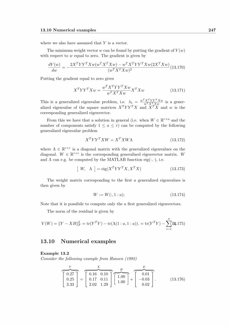
13.10 Numerical examples 247
where we also have assumed that Y is a vector.
The minimum weight vector w can be found by putting the gradient of V (w)with respect to w equal to zero. The gradient is given by
dV (w)dw
= −2XT Y Y T Xw(wT XT Xw)− wT XT Y Y T Xw(2XT Xw)(wT XT Xw)2
(13.170)
Putting the gradient equal to zero gives
XT Y Y T Xw =wT XT Y Y T Xw
wT XT XwXT Xw (13.171)
This is a generalized eigenvalue problem, i.e. λ1 = wT XT Y Y T XwwT XT Xw
is a gener-alized eigenvalue of the square matrices XT Y Y T X and XT X and w is thecorresponding generalized eigenvector.
From this we have that a solution in general (i.e. when W ∈ Rr×a and thenumber of components satisfy 1 ≤ a ≤ r) can be computed by the followinggeneralized eigenvalue problem
XT Y Y T XW = XT XWΛ (13.172)
where Λ ∈ Rr×r is a diagonal matrix with the generalized eigenvalues on thediagonal. W ∈ Rr×r is the corresponding generalized eigenvector matrix. Wand Λ can e.g. be computed by the MATLAB function eig(·, ·), i.e.
[W, Λ
]= eig(XT Y Y T X,XT X) (13.173)
The weight matrix corresponding to the first a generalized eigenvalues isthen given by
W := W (:, 1 : a); (13.174)
Note that it is possibile to compute only the a first generalized eigenvectors.
The norm of the residual is given by
V (W ) = ‖Y −XB‖2F = tr(Y T Y )− tr(Λ(1 : a, 1 : a)). = tr(Y T Y )−
a∑
i=1
λi(13.175)
13.10 Numerical examples
Example 13.2Consider the following example from Hansen (1992)
Y︷ ︸︸ ︷
0.270.253.33
=
X︷ ︸︸ ︷
0.16 0.100.17 0.112.02 1.29
B︷ ︸︸ ︷[1.001.00
]+
E︷ ︸︸ ︷
0.01−0.03
0.02
. (13.176)
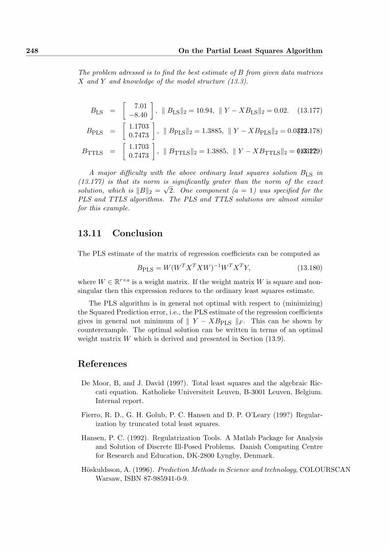
248 On the Partial Least Squares Algorithm
The problem adressed is to find the best estimate of B from given data matricesX and Y and knowledge of the model structure (13.3).
BLS =[
7.01−8.40
], ‖ BLS‖2 = 10.94, ‖ Y −XBLS‖2 = 0.02. (13.177)
BPLS =[
1.17030.7473
], ‖ BPLS‖2 = 1.3885, ‖ Y −XBPLS‖2 = 0.0322.(13.178)
BTTLS =[
1.17030.7473
], ‖ BTTLS‖2 = 1.3885, ‖ Y −XBTTLS‖2 = 0.0322.(13.179)
A major difficulty with the above ordinary least squares solution BLS in(13.177) is that its norm is significantly grater than the norm of the exactsolution, which is ‖B‖2 =
√2. One component (a = 1) was specified for the
PLS and TTLS algorithms. The PLS and TTLS solutions are almost similarfor this example.
13.11 Conclusion
The PLS estimate of the matrix of regression coefficients can be computed as
BPLS = W (W T XT XW )−1W T XT Y, (13.180)
where W ∈ Rr×a is a weight matrix. If the weight matrix W is square and non-singular then this expression reduces to the ordinary least squares estimate.
The PLS algorithm is in general not optimal with respect to (minimizing)the Squared Prediction error, i.e., the PLS estimate of the regression coefficientsgives in general not minimum of ‖ Y − XBPLS ‖F . This can be shown bycounterexample. The optimal solution can be written in terms of an optimalweight matrix W which is derived and presented in Section (13.9).
References
De Moor, B, and J. David (199?). Total least squares and the algebraic Ric-cati equation. Katholieke Universiteit Leuven, B-3001 Leuven, Belgium.Internal report.
Fierro, R. D., G. H. Golub, P. C. Hansen and D. P. O’Leary (199?) Regular-ization by truncated total least squares.
Hansen, P. C. (1992). Regulatrization Tools. A Matlab Package for Analysisand Solution of Discrete Ill-Posed Problems. Danish Computing Centrefor Research and Education, DK-2800 Lyngby, Denmark.
Hoskuldsson, A. (1996). Prediction Methods in Science and technology, COLOURSCANWarsaw, ISBN 87-985941-0-9.
13.12 Appendix: proofs 249
13.12 Appendix: proofs
13.12.1 Proof of Equation (13.115)
The Squared Prediction error (SPE) can be expressed as
VN (B) =‖ Y − TCT ‖2F = tr{(Y − TCT )T (Y − TCT )}
= tr{(Y T − CSΛ−1t T T )(Y − TΛ−T
t ST CT )},(13.181)
where we have used Equation (13.78). We have
VN (B) =‖ Y − TCT ‖2F = tr(Y T Y )− 2tr(CSΛ−1
t T T Y ) + tr(CSΛ−1t T T TΛ−T
t ST CT ),(13.182)
and
VN (B) = tr(Y T Y )− 2tr(SΛ−1t T T Y C) + tr(Λ−1
t ST CT CS) (13.183)
We have from Definition 13.2 and Remark 13.4 that the diagonal of matrixM = T T Y C = T T U is equal to the diagonal of matrix S. We also have thatthe matrix CT C have ones on the diagonal, S is a diagonal matrix and Λt is adiagonal matrix. This gives
VN (B) = tr(Y T Y )− 2tr(S2Λ−1t ) + tr(Λ−1
t S2) = tr(Y T Y )− tr(Λ−1t S2).(13.184)
QED.
Note that a general condition for PLS is given by
SCT = T T Y. (13.185)
This condition is to our knowledge new. Equation (13.185) can be derived byputting the gradient matrix dVN (B)/dtr(C) = 0, i.e., putting the gradient ma-trix of (13.183) to zero. Using this condition we derive the following expressionfor the decomposition of Y
Y = TΛ−1t T T Y + F. (13.186)
Hence, the projection of the row space of Y T onto the row space of T T is equalto
Y T /T T = Y T TΛ−1t T T , (13.187)
and, similarly
T\Y = TΛ−1t T T Y = ToT
To Y. (13.188)
Using (13.185) the SPE can be written as
VN = tr(Y T Y )− tr(Y T TΛ−1t T T Y ). (13.189)
250 On the Partial Least Squares Algorithm
The second term on the right hand side is related to the SVD of Λ− 1
2t T T Y .
Define
Λ− 1
2t T T Y = T T
o Y = U SVT . (13.190)
Then,
VN = tr(Y T Y )−min(a,m)∑
i=1
s2i . (13.191)
Note also the following alternative expression for the PLS regression matrix
BPLS = W (P T W )−1(T T T )−1T T Y. (13.192)
A proof is given as follows
T\Y = XBPLS = TΛ−1t T T Y = TP T︸ ︷︷ ︸
X
W (P T W )−1(T T T )−1T T Y︸ ︷︷ ︸BPLS
. (13.193)
13.12.2 The PLS algorithm in terms of the W weight matrix
The results in this section is of interest sinse it shows that the entire PLSalgorithm is dependent on the weight matrix W , only. We have the followingresults.
The PLS prediction of Y can be expressed as
Y = XW (W T XT XW )−1W T XT Y. (13.194)
This result can be proved by combining Y = T (T T T )−1T T Y and T = XW (T T XW )−1Λt.
Comparing this with Y = XBPLS gives
BPLS = W (W T XT XW )−1W T XT Y. (13.195)
Similarly as (13.194), the PLS prediction of X can be expressed as
X = XW (W T XT XW )−1W T XT X. (13.196)
The above result are important since it shows that the PLS estimate ofB can be computed from X, Y and the weight matrix W , only. The onlyproblem is how to compute the weight matrix W . The PLS techique is onlyone approach.
Note also that if W is an arbitrary but square non-singular matrix, then(13.195) reduces to the ordinary least squares (LS) solution. This shows that thePLS estimate is equivalent to the LS solution when the number of componentsis a = r.
13.12 Appendix: proofs 251
An expression for the rank one reduction of X in PLS can be derived fromthe equation for the residual
G = X −XW (W T XT XW )−1W T XT X. (13.197)
Similarily, for the outputs
F = Y −XW (W T XT XW )−1W T XT Y. (13.198)
The consequense of this is that the SPE is
VN (B) = ‖ Y − Y ‖2F =‖ Y −XBPLS ‖2
F
= tr(Y T Y )− tr(Y T Y )= tr(Y T Y )− tr(Y T XW (W T XT XW )−1W T XT Y ). (13.199)

252 On the Partial Least Squares Algorithm
13.13 Matlab code: The PLS1 algorithm

13.14 Matlab code: The PLS2 algorithm 253
13.14 Matlab code: The PLS2 algorithm

254 On the Partial Least Squares Algorithm
13.15 Matlab code: The PLS3 algorithm
Appendix A
Proof of the ESSM
A.1 Proof of the ESSM
The common equation in subspace identification is derived from the linear statespace model and given by
yk|L = OLxk +HdLuk|L (A.1)
The scalar positive integer parameter L can be viewed as the horizon necessaryfor the observability matrix OL to be of rank n. Hence L ≥ n− rank(D) + 1 inorder for the state space vector xk to be identified from Equation (A.1). Thusit make sense to define L as the identification horizon.
Equation (A.1) can be used to predict M steps into the future. AssumeM ≥ 1. We have
yk+M |L = OLxk+M +HdLuk+M |L (A.2)
The state space vector in the future xk+M is related to the present state xk
through the state equation. Hence we have
xk+M = AMxk + CdM uk|M (A.3)
Substituting Equation (A.3) into (A.2) gives
yk+M |L = OLAMxk +OLCdM uk|M +Hd
Luk+M |L (A.4)
The present state xk is determined from Equation (A.1) and given by
xk = O†(yk|L −HdLuk|L) (A.5)
Finally, substituting xk defined in equation (A.5) into (A.4) gives
yk+M |L = OLAMO†L(yk|L −HdLuk|L) +OLCd
M uk|M +HdLuk+M |L (A.6)
256 Proof of the ESSM
which can be written as
yk+M |L = AML yk|L + BL|L+M uk|L+M + CL|L+M ek|L+M (A.7)
BL|L+M =[ OLCd
M HdL
]− [AM
L HdL 0Lm×Mr
](A.8)
CL|L+M =[ OLCs
M HsL
]− [AM
L HsL 0Lm×Mm
](A.9)
AML = OLAMO†L (A.10)
The ESSM model correspond to Equation (A.7) with M = 1 and k ≥ L. Thepast inputs and outputs, 0 ≤ k < L, is used as instruments to remove futurenoise.
A.2 Discussion
An interesting result is obtained by choosing M = L. In this case the toeplizmatrix Hd
L can be determined directly if the inputs are sufficiently exiting.
Consider the case in which M = L, then
Yk+L|L = ALLYk|L + BLUk|2L + CLEk|2L (A.11)
BL =[ OLCL − AL
LHdL Hd
L
](A.12)
CL =[ OLCL − AL
LHsL Hs
L
](A.13)
A.3 Selector matrices
Our experience is that the choice of the parameter L (number of block rows inthe extended observability matrix) should be chosen as small as possibile. I.e.close to the minimal value in order to ensure observability.
The reason for this is twofold. First, the computational expence will increasewhen L is increased. Second, for porely exiting input signals, we avoid (pseudo)inversion of badly conditioned Hankel matrices when L is small. This willusually influence on the variance of the parameter estimates.
Syyk+M |L = AMp Syyk|L + BpSuuk|L+M + CpSeek|L+M (A.14)
AMp = SyA
ML S†y (A.15)
Bp = SyBLS†u (A.16)Cp = SyCLS†e (A.17)
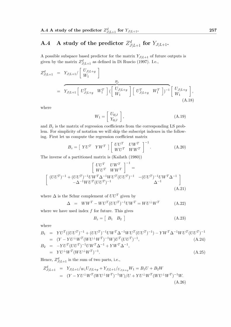
A.4 A study of the predictor ZdJ |L+1 for YJ |L+1. 257
A.4 A study of the predictor ZdJ |L+1 for YJ |L+1.
A possible subspace based predictor for the matrix YJ |L+1 of future outputs isgiven by the matrix Zd
J |L+1 as defined in Di Ruscio (1997). I.e.,
ZdJ |L+1 = YJ |L+1/
[UJ |L+g
W1
]
=
Bz︷ ︸︸ ︷YJ |L+1
[UT
J |L+g W T1
]([
UJ |L+g
W1
] [UT
J |L+g W T1
])−1
[UJ |L+g
W1
],
(A.18)
where
W1 =[
U0|JY0|J
], (A.19)
and Bz is the matrix of regression coefficients from the corresponding LS prob-lem. For simplicity of notation we will skip the subscript indexes in the follow-ing. First let us compute the regression coefficient matrix
Bz =[
Y UT Y W T] [
UUT UW T
WUT WW T
]−1
. (A.20)
The inverse of a partitioned matrix is (Kailath (1980))[
UUT UW T
WUT WW T
]−1
=[
(UUT )−1 + (UUT )−1UW T ∆−1WUT (UUT )−1 −(UUT )−1UW T ∆−1
−∆−1WUT (UUT )−1 ∆−1
]
(A.21)
where ∆ is the Schur complement of UUT given by
∆ = WW T −WUT (UUT )−1UW T = WU⊥W T (A.22)
where we have used index f for future. This gives
Bz =[
B1 B2
](A.23)
where
B1 = Y UT ((UUT )−1 + (UUT )−1UW T ∆−1WUT (UUT )−1)− Y W T ∆−1WUT (UUT )−1
= (Y − Y U⊥W T (WU⊥W T )−1W )UT (UUT )−1, (A.24)B2 = −Y UT (UUT )−1UW T ∆−1 + Y W T ∆−1,
= Y U⊥W T (WU⊥W T )−1. (A.25)
Hence, ZdJ |L+1 is the sum of two parts, i.e.,
ZdJ |L+1 = YJ |L+1/W1UJ |L+g + YJ |L+1/UJ|L+g
W1 = B1U + B2W
= (Y − Y U⊥W T (WU⊥W T )−1W )/U + Y U⊥W T (WU⊥W T )−1W.
(A.26)

258 Proof of the ESSM
Appendix B
Linear Algebra and MatrixCalculus
B.1 Trace of a matrix
The trace of a n ×m matrix A is defined as the sum of the diagonal elementsof the matrix, i.e.
tr(A) =n∑
i=1
aii (B.1)
We have the following trace operations on two matrices A and B of apropriatedimensions
tr(AT ) = tr(A) (B.2)tr(ABT ) = tr(AT B) = tr(BT A) = tr(BAT ) (B.3)tr(AB) = tr(BA) = tr(BT AT ) = tr(AT BT ) (B.4)
tr(A±B) = tr(A)± tr(B) (B.5)
B.2 Gradient matrices
∂∂X tr[X] = I (B.6)∂
∂X tr[AX] = AT (B.7)∂
∂X tr[AXT ] = A (B.8)∂
∂X tr[AXB] = AT BT (B.9)∂
∂X tr[AXT B] = BA (B.10)∂
∂X tr[XX] = 2XT (B.11)∂
∂X tr[XXT ] = 2X (B.12)
260 Linear Algebra and Matrix Calculus
∂∂X tr[Xn] = n(Xn−1)T (B.13)∂
∂X tr[AXBX] = AT XT BT + BT XT AT (B.14)∂
∂X tr[eAXB] = (BeAXBA)T (B.15)
∂
∂Xtr[XAXT ] = 2XA, if A = AT (B.16)
∂∂XT tr[AX] = A (B.17)
∂∂XT tr[AXT ] = AT (B.18)
∂∂XT tr[AXB] = BA (B.19)
∂∂XT tr[AXT B] = AT BT (B.20)
∂∂XT tr[eAXB] = BeAXBA (B.21)
B.3 Derivatives of vector and quadratic form
The derivative of a vector with respect to a vector is a matrix. We have thefollowing identities:
∂x∂xT = I (B.22)∂∂x (xT Q) = Q (B.23)∂∂x (Qx) = QT (B.24)
(B.25)
The derivative of a scalar with respect to a vector is a vector. We have thefollowing identities:
∂∂x (yT x) = y (B.26)∂∂x (xT x) = 2x (B.27)∂∂x (xT Qx) = Qx + QT x (B.28)∂∂x (yT Qx) = QT y (B.29)
Note that if Q is symmetric then∂
∂x(xT Qx) = Qx + QT x = 2Qx. (B.30)
B.4 Matrix norms
The trace of the matrix product AT A is related to the Frobenius norm of A asfollows
‖A‖2F = tr(AT A), (B.31)
where A ∈ RN×m.
B.5 Linearization 261
B.5 Linearization
Given a vector function f(x) ∈ Rm where x ∈ Rn. The derivative of the vectorf with respect to the row vector xT is defined as
∂f
∂xT=
∂f1
∂x1
∂f1
∂x2· · · ∂f1
∂xn∂f2
∂x1
∂f2
∂x2· · · ∂f2
∂xn...
.... . .
...∂fm
∂x1
∂fm
∂x2· · · ∂fm
∂xn
∈ Rm×n (B.32)
Given a non-linear differentiable state space model
x = f(x, u), (B.33)y = g(x). (B.34)
A linearized model around the stationary points x0 and u0 is
˙δx = Ax + Bu, (B.35)δy = Dx, (B.36)
where
A =∂f
∂xT|x0,u0 , (B.37)
B =∂f
∂uT|x0,u0 , (B.38)
D =∂g
∂xT|x0,u0 , (B.39)
and where
x = x− x0, (B.40)u = u− u0. (B.41)
B.6 Kronecer product matrices
Given a matrix X ∈ RN×r. Let Im be the (m×m) identity matrix. Then
(X ⊗ Im)T = XT ⊗ Im, (B.42)
(Im ⊗X)T = Im ⊗XT . (B.43)

262 Linear Algebra and Matrix Calculus
Appendix C
Optimization of the DSRalgorithm
C.1 Existence of an optimal solution
For a given pair (D,A) there exists a canonical form (Dc, Ac) where Dc consistof only ones and zeroes and with a minimal number of free parameters in Ac.Denote the free parameters as
θA = css(A) (C.1)
where css(·) is defined as the column structure string operator. See Di Ruscio(1993) p. 121.
The problem of identifying the poles as well as the system matrices D andA is reduced to solving the following optimization problem.
minθA
‖R42 −OLA(OTLOL)−1OT R32‖F (C.2)
where ‖ · ‖F is the matrix Frobenius norm.
The size of this optimization problem can be further reduced. Define theSVD
R32 = USV T (C.3)
The Frobenius norm is invariant under orthogonal transformations. See Goluband Loan (1883) p. 15. Then we have
minθA
‖R42V −OLA(OTLOL)−1OT US‖F (C.4)
Monte Carlo simulations shows that this solution is optimal and different fromthe original DSR algorithm.
Note also that A can be computed from the following least squares problem
cs(R42) =[
((OTLOL)−1OT R32)T ⊗OL
]cs(A) (C.5)
264 Optimization of the DSR algorithm
C.2 Optimized algorithm for computing the B andE matrices
In the DSR algorithm the system order and the matrices D and A are computedin a first step. There are many alternatives for computing the system matricesB and E from known D and A. One alternative to the one presented in DiRuscio (1995) is given in the following. A similar strategy for computing the Band E matrices for SISO systems is presented in the covariance based methodin Di Ruscio (1993) p. 50. Monte Carlo simulations of combined deterministicand stochastic systems shows that the algorithm improves the accuracy of theB E estimates compared to the original DSR algorithm. The method is optimalin a least squares sense, i.e., the parameters in B and E are computed from aleast squares optimal solution. Note that the algorithms gives the same resultin the purely deterministic case.
From the DSR algorithm we have the matrix equation
M = BLR11, (C.6)
where
Mdef= R41 − ALR31 ∈ RLm×(L+g)r (C.7)
and
AL = OLA(OTLOL)−1OT
L ∈ RLm×Lm. (C.8)
The matrices R41 ∈ RLm×(L+g)r, R31 ∈ RLm×(L+g)r and R11 ∈ R(L+g)r×(L+g)r
in Equations (C.6) and (C.7) are submatrices from the lower Left, Q-orthogonal(LQ) decomposition.
The matrix equation (C.6) can be solved for BL for known matrices M andR11 provided R11 is non-singular. The matrices B and E can be computed fromBL when A and D are known. In Di Ruscio (1995) a variant of this strategywhich only have to invert a submatrix of R11 of size (n− rank(D) + 1 + g)r ispresented.
In the following an alternative and optimal method for computing the Band E matrices are presented. For given system matrices D and A the matrixBL is a function of the unknown matrices B and E. We will show that Equation(C.6) can be written as a least squares problem for the unknown parameters inB and E.
In the following a proper state space model with E 6= 0m×r is assumed.From the definition we recall that g = 1 for this case. Define
Ndef=
L+g∑
i=1
RTi ⊗ (Ei−1 − ALEi) ∈ RLm(L+g)r×(n+gm)r (C.9)
where ⊗ denotes the Kronecker tensor product. The matrices Ri and Ei aredefined below. We then have the following least squares problem for computing
C.2 Optimized algorithm for computing the B and E matrices 265
the B and E matrices.
cs(M) = Ncs([
BE
]) (C.10)
where cs(·) is the column string operator, i.e. a column vector constructed bystacking the columns of a matrix on each other. The matrix N is determinedfrom the term BLR32 by extensive use of the identity
cs(AXB) = (BT ⊗A)cs(X)
for the column string operation of the product of a triple matrices A, X and Bof appriopriate dimensions (Vetter (1970)).
Then we have the least squares solution
cs([
BE
]) = N †cs(M) (C.11)
where N † = (NT N)−1NT is the Moore-Penrose pseudo-inverse of N .
The matrices
Ri ∈ Rr×(L+g)r ∀ i = 1, · · · , L + g
are block rows in the R11 ∈ R(L+g)r×(L+g)r matrix. The matrices
Ei−1 ∈ RLm×(n+mg) ∀ i = 1, · · · , L + g
are defined as follows
E0 =[
OL 0Lm×m
], EL+1 = 0Lm×(n+m), (C.12)
E1 =
0m×n Im×m
D 0m×m
DA 0m×m...
...DAL−2 0m×m
, E2 =
0m×n 0m×m
0m×n Im×m
D 0m×m...
...DAL−3 0m×m
, EL =
0m×n 0m×m
0m×n 0m×m
0m×n 0m×m...
...0m×n Im×m
.(C.13)
Some examples are presented in the following in order to illustrate the abovemethod for computing the B and E matrices.
Example C.1Considder the equation
Z = Hd3U0|3 (C.14)
and the problem of computing B and E from known matrices Z, U0|3, D andA. We have
Z =
Hd3︷ ︸︸ ︷
E 0m×r 0m×r
DB E 0m×r
DAB DB E
U1
U2
U3
(C.15)
266 Optimization of the DSR algorithm
and
Z =
0m×n Im×m
D 0m×m
DA 0m×m
[BE
]U1 +
0m×n 0m×m
0m×n Im×m
D 0m×m
[BE
]U2 +
0m×n 0m×m
0m×n 0m×m
0m×n Im×m
[BE
]U3(C.16)
Then we have
cs(Z) = Ncs([
BE
]) (C.17)
where
N = UT1 ⊗
0m×n Im×m
D 0m×m
DA 0m×m
+ UT
2 ⊗
0m×n 0m×m
0m×n Im×m
D 0m×m
+ UT
3 ⊗
0m×n 0m×m
0m×n 0m×m
0m×n Im×m
(C.18)
Example C.2Considder the ESSM with L = 1 and g = 1, i.e.
Y1|1 = A1Y0|1 + B1U0|2 (C.19)
Assume that the input and output data as well as A1 are known. Define
M = Y1|1 − A1Y0|1 (C.20)
Then we have the matrix equation
M = B1U0|2 (C.21)
Problem: Compute B and E from known matrices M , A1 and U0|2.Solution: We have
M =
B1︷ ︸︸ ︷([
DB E]− A1
[E 0m×r
])[
U1
U2
](C.22)
The matrix B1 can be written as follows
B1 =[
DB − A1E E]
(C.23)
From this we have
M = (E0 − A1E1)[
BE
]U1 + E1
[BE
]U2 (C.24)
where
E0 =[
D 0m×m
], E1 =
[0m×n Im×m
]. (C.25)
This gives the least squares problem
cs(M) = Ncs([
BE
]) (C.26)
where
N = UT1 ⊗ (E0 − A1E1) + UT
2 ⊗ E1 (C.27)
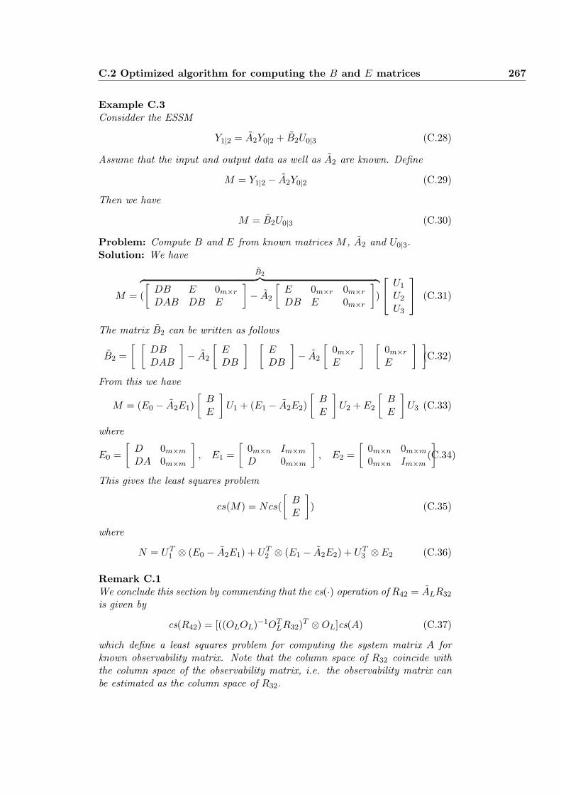
C.2 Optimized algorithm for computing the B and E matrices 267
Example C.3Considder the ESSM
Y1|2 = A2Y0|2 + B2U0|3 (C.28)
Assume that the input and output data as well as A2 are known. Define
M = Y1|2 − A2Y0|2 (C.29)
Then we have
M = B2U0|3 (C.30)
Problem: Compute B and E from known matrices M , A2 and U0|3.Solution: We have
M =
B2︷ ︸︸ ︷([
DB E 0m×r
DAB DB E
]− A2
[E 0m×r 0m×r
DB E 0m×r
])
U1
U2
U3
(C.31)
The matrix B2 can be written as follows
B2 =[ [
DBDAB
]− A2
[EDB
] [EDB
]− A2
[0m×r
E
] [0m×r
E
] ](C.32)
From this we have
M = (E0 − A2E1)[
BE
]U1 + (E1 − A2E2)
[BE
]U2 + E2
[BE
]U3 (C.33)
where
E0 =[
D 0m×m
DA 0m×m
], E1 =
[0m×n Im×m
D 0m×m
], E2 =
[0m×n 0m×m
0m×n Im×m
](C.34)
This gives the least squares problem
cs(M) = Ncs([
BE
]) (C.35)
where
N = UT1 ⊗ (E0 − A2E1) + UT
2 ⊗ (E1 − A2E2) + UT3 ⊗E2 (C.36)
Remark C.1We conclude this section by commenting that the cs(·) operation of R42 = ALR32
is given by
cs(R42) = [((OLOL)−1OTLR32)T ⊗OL]cs(A) (C.37)
which define a least squares problem for computing the system matrix A forknown observability matrix. Note that the column space of R32 coincide withthe column space of the observability matrix, i.e. the observability matrix canbe estimated as the column space of R32.

268 Optimization of the DSR algorithm

Appendix D
D-SR Toolbox for MATLAB
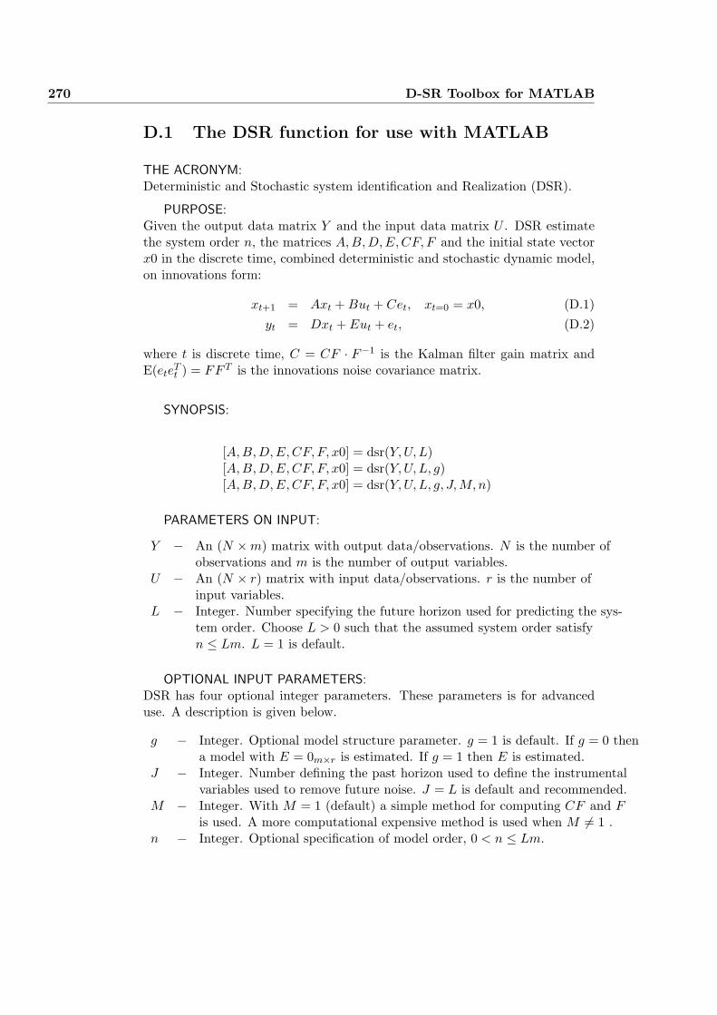
270 D-SR Toolbox for MATLAB
D.1 The DSR function for use with MATLAB
THE ACRONYM:Deterministic and Stochastic system identification and Realization (DSR).
PURPOSE:Given the output data matrix Y and the input data matrix U . DSR estimatethe system order n, the matrices A,B, D, E,CF, F and the initial state vectorx0 in the discrete time, combined deterministic and stochastic dynamic model,on innovations form:
xt+1 = Axt + But + Cet, xt=0 = x0, (D.1)yt = Dxt + Eut + et, (D.2)
where t is discrete time, C = CF · F−1 is the Kalman filter gain matrix andE(ete
Tt ) = FF T is the innovations noise covariance matrix.
SYNOPSIS:
[A,B, D, E,CF, F, x0] = dsr(Y,U, L)[A,B, D, E,CF, F, x0] = dsr(Y,U, L, g)[A,B, D, E,CF, F, x0] = dsr(Y,U, L, g, J,M, n)
PARAMETERS ON INPUT:
Y − An (N ×m) matrix with output data/observations. N is the number ofobservations and m is the number of output variables.
U − An (N × r) matrix with input data/observations. r is the number ofinput variables.
L − Integer. Number specifying the future horizon used for predicting the sys-tem order. Choose L > 0 such that the assumed system order satisfyn ≤ Lm. L = 1 is default.
OPTIONAL INPUT PARAMETERS:DSR has four optional integer parameters. These parameters is for advanceduse. A description is given below.
g − Integer. Optional model structure parameter. g = 1 is default. If g = 0 thena model with E = 0m×r is estimated. If g = 1 then E is estimated.
J − Integer. Number defining the past horizon used to define the instrumentalvariables used to remove future noise. J = L is default and recommended.
M − Integer. With M = 1 (default) a simple method for computing CF and Fis used. A more computational expensive method is used when M 6= 1 .
n − Integer. Optional specification of model order, 0 < n ≤ Lm.


![REFERENCE-BASED STOCHASTIC SUBSPACE ...people.duke.edu/~hpgavin/SystemID/References/Peeters...Peeters et al. [16] are reporting on the comparison of several output-only identi"cation](https://static.fdocuments.net/doc/165x107/612718098538f52b543bcfdf/reference-based-stochastic-subspace-hpgavinsystemidreferencespeeters-peeters.jpg)


