SUBMITTED TO IEEE TRANS. AUTOMATIC CONTROL 1

Resilient Stabilization of Switched Linear ControlSystems against Adversarial Switching

Jianghai Hu, Member, IEEE, Jinglai Shen, Senior Member, IEEE, and Donghwan Lee, Student Member, IEEE

Abstract—This paper studies the problem of stabilizingdiscrete-time switched linear control systems (SLCSs) usingcontinuous input by a user against adversarial switching by anadversary. It is assumed that at each time the adversary knowsthe user’s decision on the continuous input but not vice versa.A quantitative metric of stabilizability is proposed. Systems atthe margin of stabilizability are further classified and studied viathe notions of defectiveness and reducibility. Analytical boundson the stabilizability metric are derived using (semi)norms, withtight bounds provided by extremal norms. Numerical algorithmsare also developed for computing this metric. An applicationexample in networked control systems is presented.

Index Terms—Switched control systems, stabilization, robust-ness, resilient systems.

I. INTRODUCTION

Switched control systems are hybrid systems controlled bya continuous input signal and a switching signal (or modesequence in the discrete-time case). Stabilization of switchedcontrol systems is the problem of designing control laws forthe controllable input signals to achieve a stable closed-loopsystem [1]–[6]. The existing approaches are roughly classifiedinto two categories. In the first category (e.g., [1], [3], [4],[6], [7]), both the continuous input and the switching signalare utilized for stabilization. In the second category, the con-tinuous input is used as a control, whereas the switching signalis treated as a disturbance subject to certain constraints (e.g.,switching frequency and dwell time constraints). A commonassumption in prior work of this category (e.g., [8]–[15]) isthat the continuous controller knows exactly the current modefor at least some duration of time following each switch-ing, and hence can take the form of a collection of mode-dependent state feedback controllers. Additional assumptions(e.g., controllability of individual subsystems [9], [13], andminimal dwell time [8], [15]) are often imposed to ensure thestabilizability of the switched control systems.

The resilient stabilization problem studied in this paperbelongs to the second category but assumes a different infor-mation structure: at each time, the user decides the continuousinput without any knowledge of the current mode, whereasthe adversary is aware of the current continuous input. Thisdisadvantage for the user makes the resilient stabilization a

J. Hu and D. Lee are with the Department of Electrical andComputer Engineering, Purdue University, 465 Northwestern Ave, WestLafayette, IN, 47906 USA. Tel: (765) 496-2395, Fax: (765) 494-3371.jianghai,lee1923@purdue.edu. This material is based onwork supported by the National Science Foundation under Grant No. 1329875.

J. Shen is with the Department of Mathematics and Statistics, Universityof Maryland, Baltimore County, MD, 21250 USA. Tel: (410) 455-2402, Fax:(410) 455-1066. shenj@umbc.edu.

very challenging task. For example, even if each subsystemis stabilizable to the origin in one time step, the switchedcontrol system may not be stabilizable (see Example II.1). Ap-plications of the resilient stabilization problem include robustnetworked control systems with uncertain network delay [16]and the (stability, safety) control of survivable cyber-physicalsystems under malicious cyber attacks and sabotages [17].

The resilient stabilization problem has been addressed indifferent contexts before. It can be formulated as the robuststabilization of linear control systems with polytopic uncer-tainty. However, to our knowledge, the existing work eitherassumes uncertain but constant system matrices [18] or onlyconsiders special cases such as quadratic stabilizability [16],[19], [20] and linear control policies [21]. Other relevantresults include simultaneous stabilization of multiple linearsystems [22] and stabilization of switched systems underdelayed switching observability [13]. These results provideconservative sufficient conditions for resilient stabilization.

The contributions of this paper are four folds: (i) Sufficientand necessary conditions as well as a quantitative metric ofresilient stabilizability are developed; (ii) SLCSs at the marginof resilient stabilizability are characterized; (iii) Theoreticalresults and numerical algorithms are developed that can pro-duce more accurate bounds on the stabilizability metric thanthe existing approaches; (iv) We show that the resiliently sta-bilizing controllers are nonlinear in general (cf. Example V.2).The results in this paper extend those on the stability ofautonomous switched linear systems (SLSs) [23]–[27] to thestabilization of SLCS using continuous control input.

This paper is organized as follows. The σ-resilient stabi-lization problem is formulated in Section II. The conceptsof nondefective and irreducible systems are introduced inSection III. In Sections IV and V, theoretical and practicalbounds on the σ-resilient stabilizing rate are established.Section VI presents an application in network control systems.Finally, concluding remarks are given in Section VII.

II. RESILIENT STABILIZABILITY

Consider the discrete-time switched linear control system(SLCS) on Rn with the state x(·) ∈ Rn:

x(t+ 1) = Aσ(t)x(t) +Bσ(t)u(t), t ∈ Z+. (1)

Here, u(·) ∈ Rp and σ(·) ∈M := 1, . . . ,m are the (contin-uous) control input and switching sequence, respectively; thesets Z+ := 0, 1, . . . and N := 1, 2, . . .. For brevity, theSLCS is denoted by (Ai, Bi)i∈M, where Ai ∈ Rn×n andBi ∈ Rn×p specify the dynamics of subsystem i.

SUBMITTED TO IEEE TRANS. AUTOMATIC CONTROL 2

The following assumption is made throughout this paper.

Assumption II.1 (Admissible Control and Switching Policies).Denote by Ft := (x0:t, u0:t−1, σ0:t−1) the causal informationavailable at time t ∈ Z+, where x0:t denotes x(0), . . . , x(t)and similarly for u0:t−1 and σ0:t−1, with the understandingthat F0 := x(0). An admissible control policy u :=u0,u1, . . . consists of a sequence of feedback control lawsut : Rn(t+1) × Rpt ×Mt → Rp so that u(t) = ut(Ft), ∀t.Denote by U the set of all admissible control policies. Anadmissible switching policy σ := (σ0, σ1, . . .) consists of asequence of feedback switching laws σt : Rn(t+1) × Rpt ×Mt × Rp → M so that the switching sequence at time t isspecified by the adversary as σ(t) = σt(Ft, u(t)). The set ofall admissible switching policies is denoted by S.

Thus, the user and the adversary are playing a dynamicgame: at each time t, the user decides u(t) first and then theadversary decides σ(t) with the full knowledge of u(t).

Denote by x(·;σ,u, z) the solution to the SLCS from theinitial state z under the control policy u ∈ U and switchingpolicy σ ∈ S. Let ‖ · ‖ be an arbitrary norm on Rn.

Definition II.1. The SLCS is called σ-resiliently exponentiallystabilizable if there exist an admissible control policy u ∈ Uand constants κ ∈ [0,∞), ρ ∈ [0, 1) such that

‖x(t;σ,u, z)‖ ≤ κρt‖z‖, ∀ t ∈ Z+,∀ z ∈ Rn,∀σ ∈ S. (2)

Definition II.2. For the SLCS (1), the infimum of all ρ ≥ 0for which (2) holds for some κ ≥ 0 and u ∈ U is calledthe σ-resilient stabilizing rate and denoted by ρ∗. An optimalcontrol (if exists) is a u ∈ U such that (2) holds for ρ = ρ∗.

Note that ρ∗ ∈ [0,∞) provides a quantitative metricof the σ-resilient exponential stabilizability and its value isindependent of the choice of the norm ‖ · ‖. The SLCS isσ-resiliently exponentially stabilizable if and only if ρ∗ < 1.

When studying the σ-resilient stabilizability, the set S ofadversarial switching policies can be equivalently replacedwith the smaller set M∞ of all open-loop switching policies,namely, switching sequences that are determined at timet = 0. This is because whenever a switching policy σ ∈ Sdestabilizes the SLCS, so does at least one switching sequencein M∞, namely, the one actually produced by the policy σ.Hence, in the rest of this paper, we assume S = M∞ andthink of σ ∈ S as switching sequences.

As a related notion, the σ-resiliently asymptotical stabiliz-ability of the SLCS (1) is defined as the existence of u ∈ Usuch that x(t;σ,u, z) → 0 as t → ∞ for all z ∈ Rn andσ ∈ S. The following result is proved in Appendix A.

Theorem II.1. The SLCS (1) is σ-resiliently asymptoticallystabilizable if and only if it is σ-resiliently exponentiallystabilizable.

The rest of the paper will focus on the σ-resilient (expo-nential) stabilizability and the stabilizing rate ρ∗ for the SLCS(1). We first establish a homogeneous property of ρ∗.

Lemma II.1. Let ρ∗ be the σ-resilient stabilizing rate of theSLCS (Ai, Bi)i∈M. For any α, β ∈ R with β 6= 0, the SLCS(αAi, βBi)i∈M has the σ-resilient stabilizing rate |α| · ρ∗.

Proof. This result is trivial if α = 0. When α 6= 0, the conclu-sion follows directly from the observation that the scaled SLCS(Ai = αAi, Bi = βBi)i∈M has the solution x(t;σ, u, z) =αt · x(t;σ,u, z) where ut = β−1αt+1ut,∀ t, z, σ.

When all Bi = 0, the σ-resilient stabilizability is reducedto the stability of the resulting autonomous SLS defined byAii∈M under arbitrary switching, and ρ∗ becomes the jointspectral radius (JSR) [28] of the matrix set Aii∈M. Moregenerally, under a static linear state feedback control policyu(t) = Kx(t), the ρ∗ of the closed-loop system is the JSR ofAi+BiKi∈M. Note that the smallest possible JSR of Ai+BiKi∈M achieved by all gain matrices K is a conservativeestimate of the ρ∗ of the SLCS (1), since the optimal controlpolicies are nonlinear in general (see Example V.2).

Example II.1. Consider a one-dimensional (1D) SLCS on Rwith two subsystems, where A1 = a1, B1 = b1, A2 = a2, andB2 = b2 are real numbers with b21 + b22 6= 0. At any time t,given the state x(t) ∈ R, the optimal control u∗(t) can beshown to achieve the following infimum:

infu(t)∈R

max|a1x(t) + b1u(t)|, |a2x(t) + b2u(t)|

=|a1b2 − a2b1||b1|+ |b2|

|x(t)| := ρ∗ · |x(t)|, (3)

which also specifies the σ-resilient stabilizing rate ρ∗. Indeed,the optimal control u∗(t) is −[(a1 − a2)/(b1 − b2)]x(t) ifb1b2 < 0 and −[(a1 + a2)/(b1 + b2)]x(t) if b1b2 > 0. Ifb1 = 0, then u∗(t) can be any value between (a1−a2)x(t)/b2and −(a1 + a2)x(t)/b2. A similar result holds when b2 = 0.

If a1a2b1b2 ≤ 0, then ρ∗ in (3) is between the stabilizingrates |a1| and |a2| of the two autonomous subsystems. Ifa1a2b1b2 > 0, then ρ∗ can be smaller than both |a1| and |a2|.For instance, ρ∗ = 0 if a1/b1 = a2/b2, i.e., the two subsystemsare scaled versions of each other. Indeed, from any x(0), thecontrol u∗(0) = −(a1/b1)x(0) = −(a2/b2)x(0) ensures thatx(1) = 0 regardless of σ(0). Finally, since b1b2 6= 0, both thesubsystems are controllable hence stabilizable; however, theSLCS may not be σ-resiliently exponentially stabilizable.

Remark II.1. In the above example, the optimal user controlpolicy u is of the static state feedback form ut(Ft) = g(x(t)).That ut depends solely on x(t) is not surprising since thestabilizability property is entirely based on the behavior (i.e.,convergence) of the future state solution, which depends onthe past u, σ, and x only through the current state x(t). Theadversary will not gain any further advantage by knowingthe user’s optimal feedback control policy in advance. Thisobservation remains valid for all the subsequent examples inthis paper. On the other hand, if the user adopts an open-loopcontrol policy (i.e., a control sequence), then the adversaryby knowing such a sequence in advance will have a muchgreater advantage. In fact, it would be impossible to stabilizethe SLCS in Example II.1 in the latter setting.

III. DEFECTIVENESS AND REDUCIBILITY

In this section, we study those SLCSs whose σ-resilientstabilizing rates ρ∗ can be exactly achieved.

SUBMITTED TO IEEE TRANS. AUTOMATIC CONTROL 3

Definition III.1 (Defectiveness). The SLCS is called nonde-fective if there exist a control policy u ∈ U and a constantκ ≥ 0 such that ‖x(t;σ,u, z)‖ ≤ κ(ρ∗)t‖z‖, ∀ t ∈ Z+,∀ z ∈ Rn, ∀σ ∈ S. Otherwise, it is called defective.

The notion of defectiveness helps to further distinguish theσ-resilient stabilizability of those SLCSs at the margin (i.e.,with ρ∗ = 1). The SLCS is called σ-resiliently Lyapunovstabilizable if there exist u ∈ U and κ ∈ [0,∞) such that‖x(t;σ,u, z)‖ ≤ κ‖z‖,∀ t ∈ Z+, ∀ z ∈ Rn, ∀σ ∈ S .By Definition III.1, the σ-resilient Lyapunov stabilizability isequivalent to either of the following two cases: (i) ρ∗ < 1;(ii) ρ∗ = 1 and the SLCS is nondefective.

An SLCS with ρ∗ = 0 is nondefective if and only if it isresiliently controllable to the origin in one time step: for anyz ∈ Rn, there exists v ∈ Rp such that Aiz+Biv = 0, ∀i ∈M;or equivalently, Ai = BiK, ∀i ∈M, for some matrix K.

As an example, consider the LTI system (A,B), where A =[1 10 1

]and B =

[00

]. As B is zero, ρ∗ = 1 is the spectral

radius of A. Since x(t) = Atx(0) is unbounded for some x(0),the SLCS is defective. For another example, consider the LTI

system (A,B) with A =

[1 00 0

]and B =

[11

], which is

controllable to the origin in two (but not one) steps. Thus, thesystem has ρ∗ = 0 and is defective.

Tests for defectiveness are difficult to obtain. We establisheasily verified conditions for (non-)defectiveness as follows.

Definition III.2. A subset V ⊂ Rn is called a control σ-invariant set if for any z ∈ V , there exists v ∈ Rp such thatAiz + Biv ∈ V for all i ∈ M. If V is further a subspace ofRn, then it is called a control σ-invariant subspace.

Two trivial control σ-invariant subspaces are 0 and Rn.

Definition III.3 (Reducibility). The SLCS (1) is called irre-ducible if it does not have any control σ-invariant subspacesother than 0 and Rn. Otherwise, it is called reducible.

If the SLCS is reducible, then there exists a proper nontrivialcontrol σ-invariant subspace V ( Rn. After a commoncoordinate change x = T x =

[T1 T2

]x where the range

of T1 is V , the subsystem dynamics matrices of the SLCS(still denoted by Ai and Bi for simplicity) will be of the form

Ai =

[Ai,11 ∗Bi,2K Ai,22

], Bi =

[Bi,1Bi,2

], ∀ i ∈M, (4)

where ∗ indicates a matrix of proper size and the matrix Kis independent of i. Repeating this process if possible, thesubsystem dynamics matrices will eventually have the form

Ai =

Ai,11 ∗ · · · ∗Bi,2K1 Ai,22 · · · ∗

......

. . ....

Bi,rK1 Bi,rK2 · · · Ai,rr

, Bi =

Bi,1Bi,2

...Bi,r

(5)

for some matrices K1, . . . ,Kr−1, where each of the SLCSs(Ai,jj , Bi,j)i∈M is irreducible for j = 1, . . . , r. By the

change of variables u = u −[K1 · · · Kr−1 0

]x, we

derive the following standard form of reducible SLCSs:

Ai =

Ai,11 ∗ · · · ∗

0 Ai,22 · · · ∗...

.... . .

...0 0 . . . Ai,rr

, Bi =

Bi,1Bi,2

...Bi,r

, (6)

where for each j = 1, . . . , r, the SLCS (Ai,jj , Bi,ji∈M isirreducible. Clearly, the SLCSs (5) and (6) have the same σ-resilient stabilizing rate ρ∗ as that of (1).

If an SLCS has ρ∗ = 0 and is nondefective, then anysubspace of Rn will be control σ-invariant; thus the system isreducible if its state dimension is greater than one.

Assume ρ∗ > 0. Define an extended real valued functionζ : Rn → R+ ∪ ∞ as

ζ(z) := infu∈U

supσ∈S

supt∈Z+

‖x(t;σ,u, z)‖(ρ∗)t

, ∀ z ∈ Rn, (7)

which is positively homogeneous of degree one: ζ(αz) =αζ(z) for all α ≥ 0. Since supσ supt ‖x(t;σ,u, z)‖/(ρ∗)t isjointly convex in u and z and U is a vector space hence convex,by [29, pp. 87], ζ is convex on Rn. Thus, the set

W := z ∈ Rn | ζ(z) <∞ (8)

is a subspace of Rn. In Appendix B we will show that W iscontrol σ-invariant and that the following result holds.

Theorem III.1. An irreducible SLCS with ρ∗ > 0 is nonde-fective.

The converse of Theorem III.1 may not hold. A counterex-ample is given by the LTI system (A,B) with B = 0 andA ∈ R3×3 having two real eigenvalues 0 < λ1 < λ2 with aJordan block of order two for the eigenvalue λ1.

Remark III.1. The concepts of defectiveness and reducibilityhave been proposed in the study of the JSR and the stability ofautonomous SLS [23], [30]. They are extended to the SLCSin this paper. In particular, the proof of Theorem III.1 is anextension of that of [25, Theorem 2.1].

IV. BOUNDS ON σ-RESILIENT STABILIZING RATE

In this section, a systematic approach for deriving boundsof the σ-resilient stabilizing rate ρ∗ is developed.

A. Motivating Example

We first discuss a motivating example of the SLCSs.

Example IV.1. Consider the following SLCS on R2:

A1 =

[a1 00 f1

], B1 =

[b1g1

]; A2 =

[a2 00 f2

], B2 =

[b2g2

],

which is obtained from two 1D SLCSs (ai, bi)i=1,2 and(fi, gi)i=1,2 that share a common control input and acommon switching sequence. Denote by ρ∗, ρ∗1, and ρ∗2 theσ-resilient stabilizing rate of the 2D SLCS and the two 1DSLCSs, respectively. Obviously, ρ∗ ≥ max ρ∗1, ρ∗2.

SUBMITTED TO IEEE TRANS. AUTOMATIC CONTROL 4

In what follows, we assume that a1 6= f1 or a2 6= f2, andthat B1 and B2 are not collinear, i.e., b1g2 6= b2g1. Hencethe following two constants cannot be both zero: α := (a1 −f1)g2 − (a2 − f2)g1, and β := (a1 − f1)b2 − (a2 − f2)b1.Define two nonnegative functions V,W : R2 → R+ by

V (z) := |αz1 − βz2|, W (z) := |βz1 + αz2|, ∀ z ∈ R2,

where z = (z1, z2). Their null sets NV := z ∈ R2 |V (z) =0 and NW := z ∈ R2 |W (z) = 0 are orthogonal 1Dsubspaces. It follows from (3) and αbi − βgi = (b1g2 −b2g1)(ai − fi), ∀ i = 1, 2, that for any time t and x(t) = z,

infu(t)∈R

maxi=1,2

V (Aix(t) +Biu(t))

= infu(t)∈R

maxi=1,2

∣∣(αbi − βgi)u(t) + (αaiz1 − βfiz2)∣∣

=

∣∣∣∣∣ (αb1 − βg1)(αa2z1 − βf2z2)∑2i=1 |αbi − βgi|

− (αb2 − βg2)(αa1z1 − βf1z2)∑2i=1 |αbi − βgi|

∣∣∣∣∣=

|a1f2 − a2f1||a1 − f1|+ |a2 − f2|

· V (x(t)) := ρ0 · V (x(t)). (9)

The optimal u∗(t) achieving the above infimum is given by

u∗(t) := − (αa1z1 − βf1z2)± (αa2z1 − βf2z2)

(αb1 − βg1)± (αb2 − βg2), (10)

which is a linear state feedback controller with the sign “±”being “+” if (a1 − f1)(a2 − f2) ≥ 0 and “−” otherwise.

The result in (9) implies that NV is a control σ-invariantsubspace. Also, if at each time t, the adversary chooses σ(t) =arg maxi V (Aix(t)+Biu(t)), then V (x(t+1)) ≥ ρ0V (x(t))regardless of u(t). As V (·) is positively homogeneous of de-gree one, we conclude that x(t) cannot decay at an exponentialrate faster than ρ0 from x(0) satisfying V (x(0)) > 0, i.e.,

ρ∗ ≥ ρ0 =|a1f2 − a2f1|

|a1 − f1|+ |a2 − f2|. (11)

If the user adopts the feedback control strategy in (10), then

V (x(t+ 1)) = V (Aσ(t)x(t) +Bσ(t)u∗(t))

≤ ρ0 · V (x(t)), ∀σ(t) ∈ 1, 2, ∀x(t). (12)

When ρ0 < 1, x(t)→ NV as t→∞ for any σ ∈ S. To ensurethat x(t)→ 0, one needs in addition that x(t) will not divergealong NV . Pick any x(t) = (z1, z2) ∈ NV , i.e., αz1 = βz2. Itcan be verified that, with the sign in (10) being either “+” or“−”, we have W (Aix(t) +Biu

∗(t)) = ρi ·W (x(t)), where

ρi :=|gi(a1b2 − a2b1)− bi(f1g2 − f2g1)|

|b1g2 − b2g1|, i = 1, 2. (13)

Thus W (x(t+1)) ≤ maxρ1, ρ2·W (x(t)) regardless of σ(t).This, together with (12), implies that if maxρ0, ρ1, ρ2 < 1,then the system is σ-resiliently stabilized by u∗. In view ofTheorem II.1, we have ρ∗ < 1 if maxρ0, ρ1, ρ2 < 1. Asmaxρ0, ρ1, ρ2 has the exact same scaling properties as ρ∗

in Lemma II.1, we obtain via a scaling argument that

ρ∗ ≤ maxρ0, ρ1, ρ2. (14)

In the case ρ0 ≥ maxρ1, ρ2, ρ∗ = ρ0 by (11). For example,assume a1b2 = a2b1 and f1g2 = f2g1. By Example II.1, ρ∗1 =ρ∗2 = 0, while ρ∗ = ρ0 > 0 provided a1f2 − a2f1 6= 0.

B. Bounds via Seminorms

We now formalize the technique employed in Example IV.1.Recall that a seminorm on Rn is defined as a nonnegativefunction ξ : Rn → R+ that is convex (hence continuous) andpositively homogeneous of degree one [31]. A seminorm is anorm if it is positive definite, i.e., ξ(z) > 0 whenever z 6= 0.

Lemma IV.1. For an arbitrary seminorm ξ on Rn, let themapping T : ξ 7→ ξ] be defined by, ∀ z ∈ Rn,

ξ](z) = T [ξ](z) := infv∈Rp

maxi∈M

ξ(Aiz +Biv). (15)

More generally, for any h ∈ N, define the mapping T (h) by

T (h)[ξ](z) := infv(0)∈Rp

maxi(0)∈M

· · · infv(h−1)∈Rp

maxi(h−1)∈M

ξ

Ai(h−1) · · ·Ai(0)z +

h−1∑j=0

Ai(h−1) · · ·Ai(j+1)Bi(j)v(j)

.

Then T (ξ) and T (h)(ξ) are also seminorms on Rn, i.e., Tand T (h) are self maps of seminorms on Rn.

Proof. That ξ](·) is pointwise finite and nonnegative is ob-vious. It is convex since maxi∈M ξ(Aiz + Biv) is convexin (z, v) [29, pp. 88]. To show the homogeneity, let α 6= 0be arbitrary. By setting v′ := v/α, we have ξ](αz) =infv∈Rp maxi∈M ξ(αAiz + Biv) = infv′∈Rp maxi∈M |α| ·ξ(Aiz + Biv

′) = |α| · ξ](z). When α = 0, it is obviousfrom (15) that ξ](0) = 0. This shows that ξ] is a seminormon Rn. The proof for T (h) is similar hence omitted.

If ξ(·) = ‖ · ‖ is a norm on Rn, then ξ](·), which wedenote as ‖ · ‖], is a seminorm but not necessarily a normon Rn. For instance, if the two 1D subsystem dynamics inExample II.1 are scaled version of each other, i.e., a1/b1 =a2/b2, then | · |] ≡ 0, which is not a norm on R. Also,T (h)[ξ](z) defined above is the solution to the h-horizonproblem infu maxσ ξ(x(h;σ,u, z)) and T (h) = T if h = 1.

Lemma IV.2. Suppose ξ is a seminorm on Rn. Then for anygiven z ∈ Rn, the function f(v) := maxi∈M ξ(Aiz + Biv)attains a (possibly non-unique) minimizer in Rp.

Proof. Let V be the subspace v ∈ Rp | ξ(Biv) = 0, ∀ i ∈M and V⊥ be its orthogonal complement. Any v ∈ Rp can bedecomposed uniquely as v = v1 + v2, where v1 ∈ V and v2 ∈V⊥. Since f(v) = f(v2), v1 can be set to zero without loss ofgenerality. Define g(v2) := maxi∈M ξ(Biv2), which is a normon V⊥. Then, g(v2) ≤ maxi∈M[ξ(Aiz+Biv2)+ξ(−Aiz)] ≤f(v2)+maxi∈M ξ(Aiz). This implies that any nonempty sub-level set of f(·) (which is closed as f is continuous) restrictedto V⊥ is contained in a sub-level set of g(·) and thus boundedand compact. Since f is continuous, a minimizer exists.

Lemma IV.3. The mapping T : ξ 7→ ξ] defined in (15) hasthe following properties.

SUBMITTED TO IEEE TRANS. AUTOMATIC CONTROL 5

• (Monotonicity): For two extended real-valued seminormsξ and ξ′ with ξ ≤ ξ′, T (ξ) ≤ T (ξ′).

• (Monotone Continuity): Let (ξk)k∈N be a nonincreasingsequence of seminorms whose (pointwise) limit is denotedby ξ∞ = limk→∞ ξk. Then limk→∞ T (ξk) = T (ξ∞).

Proof. The first property is trivial. To show the second prop-erty, suppose ξk(z) ↓ ξ∞(z), ∀ z ∈ Rn. Being the pointwiselimit of the seminorms ξk, ξ∞ is also a seminorm on Rn.Let ηk := T (ξk). By Lemma IV.1 and the first property, (ηk)is a nonincreasing sequence of seminorms, whose pointwiselimit η∞ := limk→∞ ηk is also a seminorm. As ξk ≥ ξ∞,ηk ≥ T (ξ∞),∀ k, which implies η∞ ≥ T (ξ∞).

To prove the other direction, fix an arbitrary z ∈ Rn.Since ξ∞ is a seminorm, Lemma IV.2 implies that the mini-mizer v∗ = arg minv[maxi∈M ξ∞(Aiz + Biv)] exists. Sincemaxi∈M ξ∞(·) is also a pointwise limit of maxi∈M ξk(·)as k → ∞, we deduce that for any ε > 0, there ex-ists N large enough such that maxi∈M ξk(Aiz + Biv

∗) ≤maxi∈M ξ∞(Aiz +Biv

∗) + ε for all k ≥ N . Thus,

ηk(z) = infv

maxi∈M

ξk(Aiz +Biv) ≤ maxi∈M

ξk(Aiz +Biv∗)

≤ maxi∈M

ξ∞(Aiz +Biv∗) + ε = T [ξ∞](z) + ε,

for all k ≥ N . Letting k → ∞ and noting that ε > 0 isarbitrary, we have η∞(z) ≥ T [ξ∞](z) for any z ∈ Rn.

Proposition IV.1. Let ξ be a non-zero seminorm on Rn andα ≥ 0 be a constant such that ξ](·) ≥ α ξ(·). Then ρ∗ ≥ α.

Proof. Assume the adversary adopts the switching policyσ(t) = arg maxi ξ(Aix(t) + Biu(t)) at each t for any givenx(t), u(t). Hence σ ∈ S. Then from x(0) with ξ(x(0)) > 0,we have, for any u(t),

ξ(x(t+ 1)) = ξ(Aσ(t)x(t) +Bσ(t)u(t))

= maxi∈M

ξ(Aix(t) +Biu(t)) ≥ ξ](x(t)) ≥ α ξ(x(t)), ∀ t.

This shows that c‖x(t)‖ ≥ ξ(x(t)) ≥ αt · ξ(x(0)), ∀ t ∈ Z+,where c := sup‖z‖=1 ξ(z) > 0. Hence there exist no ρ < αand a constant κ > 0 so that ‖x(t)‖ ≤ κρt‖x(0)‖, ∀ t.

Proposition IV.1 has been applied in Example IV.1 withξ(·) = V (·) and α = ρ0 in equation (9).

Proposition IV.2. Let ‖·‖ be a norm on Rn such that ‖·‖] ≤β ‖ · ‖ for some β ≥ 0. Then, ρ∗ ≤ β.

Proof. Suppose the user adopts the control policy u∗(t) =ut(x(t)) := arg minv maxi∈M ‖Aix(t) + Biv‖, ∀ t, whichexists by Lemma IV.2. Then for any σ ∈ S and any t ∈ Z+,

‖x(t+ 1)‖ =∥∥Aσ(t)x(t) +Bσ(t)u

∗(t)∥∥

≤ maxi∈M

∥∥Aix(t) +Biu∗(t)

∥∥ = ‖x(t)‖] ≤ β‖x(t)‖.

This implies that ‖x(t)‖ ≤ βt‖x(0)‖, ∀ t, i.e., ρ∗ ≤ β.

The next result follows from Propositions IV.1 and IV.2.

Corollary IV.1. If α‖ · ‖ ≤ ‖ · ‖] ≤ β‖ · ‖ for some norm ‖ · ‖on Rn, then α ≤ ρ∗ ≤ β.

By using the operator T (h) instead of T and consideringper-h-step growth of the state solutions, we obtain the follow-ing result whose proof is similar hence omitted.

Proposition IV.3. Let h ∈ N. If ξ is a nonzero seminorm onRn and T (h)(ξ) ≥ αξ for some constant α ≥ 0, then ρ∗ ≥h√α. Further, if ξ is a norm on Rn and αξ ≤ T (h)(ξ) ≤ βξ

for some constants α, β ≥ 0, then h√α ≤ ρ∗ ≤ h

√β.

C. Extremal Norms

By Corollary IV.1, associated with each norm ‖ · ‖ are thefollowing lower and upper bounds of ρ∗:

α∗ := sup α ∈ R+ | α‖ · ‖ ≤ ‖ · ‖] ,β∗ := inf β ∈ R+ | ‖ · ‖] ≤ β‖ · ‖ .

A natural question arises: can such bounds be tight?

Definition IV.1. A norm ‖ · ‖ on Rn is called an (upper)extremal norm of the SLCS (1) if ‖ · ‖] ≤ ρ∗‖ · ‖.

Suppose an extremal norm ‖ · ‖ exists. Then the property‖ · ‖] ≤ ρ∗‖ · ‖ implies that there is an optimal control policy

ut(x(t)) := arg minv

maxi∈M‖Aix(t) +Biv‖, ∀x(t), ∀ t, (16)

under which we have ‖x(t+1)‖ ≤ ρ∗‖x(t)‖, hence ‖x(t)‖ ≤(ρ∗)t‖x(0)‖, ∀ t ∈ Z+, x(0) ∈ Rn, σ ∈ S . This implies thatthe SLCS is nondefective. The following theorem, proved inAppendix C, shows that the converse is also true.

Theorem IV.1. An extremal norm of the SLCS exists if andonly if the SLCS is nondefective.

We next focus on seminorms that yield tight lower bounds.

Definition IV.2. A nonzero seminorm ξ on Rn is called alower extremal seminorm if ξ](·) ≥ ρ∗ · ξ(·).

In Appendix D, we prove the following result.

Theorem IV.2. If the SLCS is nondefective, then a lowerextremal seminorm exists.

The converse of Theorem IV.2 is not true, at least whenρ∗ = 0. For example, the (non-switched) LTI system (A,B)

with A =

[1 00 0

]and B =

[11

]has ρ∗ = 0; hence

any seminorm is a lower extremal seminorm. However, asdiscussed in Section II, this system is defective.

Some norms can be both upper and lower extremal.

Definition IV.3. A norm ‖ · ‖ on Rn is called a Barabanovnorm if ‖ · ‖] = ρ∗‖ · ‖.

The following result is proved in Appendix E.

Theorem IV.3. If the SLCS is irreducible, then a Barabanovnorm exists.

In Example II.1 with a1/b1 = a2/b2, the 1D SLCS has aBarabanov norm | · |. Another example is given below.

Example IV.2. Consider the following SLCS on R2:

A1 =

[1 00 0

], B1 =

[11

]; A2 =

[0 00 1

], B2 =

[01

].

SUBMITTED TO IEEE TRANS. AUTOMATIC CONTROL 6

Fig. 1. Top: Unit ball of the norm ‖ · ‖ in Example IV.2; Bottom: v∗ forz = (1, y), ∀ y ∈ R.

Define a norm on R2 as

‖z‖ := max|z1|, γ|z2 − z1|, ∀ z ∈ (z1, z2) ∈ R2,

where γ =√

5−12 satisfies γ = 1/(γ+1). We claim that ‖·‖] =

γ‖ · ‖. By homogeneity, we only need to check this claim forz = (0, 1) and for z = (1, y) where y ∈ R. If z = (0, 1), then‖z‖ = γ, and ‖z‖] = infv max ‖(v, v)‖ , ‖(0, 1 + v)‖ =infv max |v|, γ|1 + v| = γ2 = γ‖z‖, where the minimumis achieved at v∗ = −γ2. Suppose z = (1, y). Then ‖z‖ =max1, γ|y−1|, and ‖z‖] = infv max |1 + v|, γ, γ|y + v|.• Case 1: Suppose y < −γ. Then ‖z‖ = γ|y − 1|, and‖z‖] = γ2(1− y) with v∗ = −γ − γ2y;

• Case 2: Suppose −γ ≤ y ≤ γ + 2. Then ‖z‖ = 1,and ‖z‖] = γ where v∗ can take any value betweenmax−y − 1,−γ − 1 and min−y + 1, γ − 1.

• Case 3: Suppose y > γ + 2. Then ‖z‖ = γ|y − 1|, and‖z‖] = γ2(y − 1) with v∗ = −γ − γ2y.

In Fig. 1, we plot the unit ball of ‖ · ‖ on the top, and thefunction v∗(y) at the bottom (the shaded region indicates thatthe value of v∗ is not unique). Note that the optimal controlpolicy can be chosen to be linear: u∗(t) = [−γ − γ2]x(t).

Remark IV.1. The notions of extremal and Barabanov normsare originally proposed for the study of the JSR and thestability of autonomous SLSs [23], [27], [32]. We extendthem to the resilient stabilization of the SLCS. The proofs ofTheorem IV.1 and Theorem IV.3 are inspired by those of [26,Theorem 3] and [23], respectively. See also [25, Theorem 2.1].Another relevant method is the variational approach [33].

Extremal norms can also be defined in terms of T (h).Specifically, (i) a nonzero seminorm ξ is lower h-extremalif T (h)(ξ) ≥ (ρ∗)hξ; (ii) a norm ‖ · ‖ is (upper) h-extremal

if T (h)(‖ · ‖) ≤ (ρ∗)h‖ · ‖, and it is an h-Barabanov norm ifT (h)(‖ · ‖) = (ρ∗)h‖ · ‖. Although (1-)extremal (semi)normsare also h-extremal, the converse may not be true.

D. Norms under Linear Transformations

The norm bounding techniques introduced in this section areindependent of coordinates on Rn. To see this, consider the co-ordinate change x = T x by a nonsingular matrix T ∈ Rn×n.A norm (resp. seminorm) ξ in x-coordinates is transformed byT to the norm (resp. seminorm) ξ := ξT in the x-coordinates.Denote the SLCS (Ai, Bi)i∈M in x-coordinates by S. Inx-coordinates it has the form S = (Ai, Bi)i∈M whereAi := T−1AiT and Bi := T−1Bi. Obviously, S and S havethe same σ-resilient stabilizing rate, i.e., ρ∗ = ρ∗. Similar toT defined in (15) for S, we define a mapping T for S by

T [ξ](z) := infv∈Rp

maxi∈M

ξ(Aiz + Biv), ∀ z ∈ Rn,

which satisfies T (ξ T ) = T (ξ) T . Then a seminorm ξsatisfies αξ ≤ T (ξ) ≤ βξ for some α, β ≥ 0 if and only ifξ = ξ T satisfies αξ ≤ T (ξ) ≤ βξ. In particular, if ξ isan extremal norm (resp. lower extremal seminorm, Barabanovnorm) for S, so is ξ for S.

Given two norms ξ and ξ′ on Rn, define

d(ξ, ξ′) := log

(minβ ≥ 0 | ξ′ ≤ βξmaxα ≥ 0 | ξ′ ≥ αξ

),

which measures how similar the unit balls of ξ and ξ′ are afterproper scalings. Define an equivalence relation for norms onRn as ξ ∼ ξ′ if and only if ξ′ = γξ for some γ > 0, anddenote by [ξ] the equivalent class that ξ belongs to. Then d(·, ·)specifies a metric on the family of equivalent classes of normson Rn (see [34] for a more general metric). The mapping T (orT ), which preserves this equivalent relation, can be extendedto a mapping between equivalent classes of norms.

A norm ξ∗ is a Barabanov norm of the SLCS S if and onlyif d(ξ∗, T (ξ∗)) = 0, or equivalently, if the equivalent class [ξ∗]is a fixed point of T . In the next section, we will search forBarabanov norms in various subsets K of norms. The distanced(K, ξ∗) := infd(ξ, ξ∗) | ξ ∈ K measures quantitativelyhow well norms in K approximate the Barabanov norm ξ∗ (ifexists). In practice, as ξ∗ is difficult to find or even nonexistent,one can use infξ∈K d(ξ, T (ξ)) as an indicator for the proximityof the best norms in K to being a Barabanov norm.

The following result will be useful in Section V-A.

Lemma IV.4 (Fritz John’s Theorem [35]). Let ‖ · ‖ be theEuclidean norm on Rn, and let Ke be the set of all normsof the form ‖ · ‖ T for some nonsingular T ∈ Rn×n (suchnorms are called ellipsoidal norms; see Section V-A). Then foran arbitrary norm ξ on Rn, d(Ke, ξ) ≤ log(

√n).

Indeed, one choice of the norm in Ke with the smallest d-distance to ξ is such that its unit ball is the largest ellipsoidcontained in the unit ball of ξ (see [34]).

V. COMPUTING σ-RESILIENT STABILIZING RATE

Using the results in Section IV, we now use certain familiesof norms to compute bounds on ρ∗. For a given σ-resiliently

SUBMITTED TO IEEE TRANS. AUTOMATIC CONTROL 7

stabilizable SLCS, the computed norm ‖ · ‖ can be used todevise a σ-resiliently stabilizing controller in the form of (16).

A. Ellipsoidal Norms

Denote by P0 and P0 the sets of all n×n positive definite(P.D.) and positive semidefinite (P.S.D.) matrices, respectively.We write P 0 if P ∈ P0 and P 0 if P ∈ P0. For eachP 0, ‖z‖P :=

√zTPz defines a seminorm on Rn. If P 0,

then ‖·‖P is a norm, called an ellipsoidal norm as its unit ballis an ellipsoid. Note that ‖ · ‖P = ‖ · ‖I T where T = P 1/2.

Applying the results in Section IV to the ellipsoidal norms,we obtain lower and upper bounds on ρ∗. As shown below,the best such bounds are off by at most a factor of

√n.

Proposition V.1. Let the SLCS be irreducible. Then thereexists an ellipsoidal norm ‖ · ‖P based on which the lowerbound of ρ∗ obtained from Proposition IV.1 is at least ρ∗/

√n

and the upper bound of ρ∗ obtained from Proposition IV.2 isat most

√n · ρ∗.

Proof. The irreducibility assumption implies that the SLCShas a Barabanov norm ξ∗. By Lemma IV.4, there exists anellipsoidal norm ξ = ‖ · ‖P satisfying ξ ≤ ξ∗ ≤

√n ξ.

This implies that T (ξ) ≤ T (ξ∗) = ρ∗ξ∗ ≤√n · T (ξ). In

particular, T (ξ) ≤ ρ∗ξ∗ ≤ ρ∗√n ξ and T (ξ) ≥ (ρ∗/

√n) ξ∗ ≥

(ρ∗/√n) ξ. This proves the desired results.

In Proposition V.1, both the lower and upper bounds areachieved by the same ellipsoidal norm. Using different ellip-soidal norms, one may obtain tighter bounds. Moreover, ifthe SLCS is nondefective, then only the second part of thestatement regarding the upper bound of ρ∗ holds true.

Remark V.1. By using T (h) with h > 1 and Proposition IV.3,the results in Proposition V.1 can be improved: there existsan ellipsoidal norm ξ = ‖ · ‖P satisfying [(ρ∗)h/

√n] · ξ ≤

T (h)(ξ) ≤ (ρ∗)h√n ξ, thus providing a lower bound of at

least ρ∗/ 2h√n and an upper bound of at most 2h

√n · ρ∗ for

ρ∗. For a fixed n, as h → ∞, estimate errors can be madearbitrarily small. The drawback of using a large h, however,is the much increased complexity in evaluating T (h)(ξ).

To find the bounds of ρ∗ from the ellipsoidal norms, weintroduce the following notation. Let m = |M|, and define

∆ :=θ ∈ Rm | θi ≥ 0, ∀ i ∈M,

∑i∈Mθi = 1

to be the m-simplex. For each θ ∈ ∆ and P 0, define

Γθ(P ) :=∑i∈M

θiATi PAi −

(∑i∈M

θiATi PBi

)×

(∑i∈M

θiBTi PBi

)†(∑i∈M

θiBTi PAi

), (17)

where † denotes the matrix pseudo inverse. Note that Γθ(P ) isthe (generalized) Schur complement [36, pp. 28] of the lowerright block of the following P.S.D. matrix:

Υθ(P ) :=∑i∈M

θi

[ATi PAi ATi PBiBTi PAi BTi PBi

]. (18)

From this we conclude that: (i) Γθ(P ) 0; and (ii) for a fixedP (resp. θ), Γθ(P ) is a PSD-concave mapping of θ (resp. P )into P0 under the partial order (cf. [29]). Define the set

Γ∆(P ) := Γθ(P ) | θ ∈ ∆ ⊂ P0.

Lemma V.1. For each P 0, denote ‖ · ‖P] := T (‖ · ‖P )where the operator T is defined in (15). Then, ∀ z ∈ Rn,

‖z‖P] = supθ∈∆‖z‖Γθ(P ) = sup

Q∈Γ∆(P )

‖z‖Q. (19)

Proof. It follows from (15) that (‖z‖P])2 is the optimal valueof the following optimization problem in r ∈ R and v ∈ Rp:

minimize r ≥ 0 (20)

subject to (Aiz +Biv)TP (Aiz +Biv) ≤ r, ∀ i ∈M.

By introducing the multipliers (dual variables) θi ≥ 0 for eachi ∈M, the dual problem of (20) is easily seen to be

maxθ∈∆

zTΓθ(P )z. (21)

Since the optimization problem (20) is both convex (indeed asecond order cone programming) and strongly feasible (r canbe made arbitrarily large), it has the same optimal value asthat of (21). This proves the desired result.

We now apply Proposition IV.1 to the ellipsoidal norm ‖·‖Pfor P 0. By Lemma V.1, the condition ‖ · ‖P] ≥ α‖ · ‖P isequivalent to supθ∈∆ zTΓθ(P )z ≥ α2zTPz, ∀z. A sufficientcondition for this to hold is Γθ(P ) α2P for some θ ∈ ∆,or by using the Schur complement

Υθ(P )−[α2P 0

0 0

] 0 (22)

for some θ ∈ ∆, where Υθ(P ) is defined in (18). Hence,Proposition IV.1 implies the following result.

Proposition V.2. Suppose the matrix inequality (22) holdsfor some α ≥ 0, P 0, and θ ∈ ∆. Then the σ-resilientstabilizing rate ρ∗ satisfies ρ∗ ≥ α.

If P 0 is given, then a lower bound of ρ∗ is obtained byfinding the largest possible α satisfying (22) for some θ ∈ ∆,which is a semidefinite program (SDP) that is easily solvable.To find the best such lower bound, we can solve the bilinearmatrix inequality (BMI) problem in (α2, P, θ):

maxα2≥0, P0, θ∈∆

α2, subject to the constraint (22). (23)

We next apply Proposition IV.2 to the ellipsoidal norms.Given P 0, the condition ‖ · ‖P] ≤ β‖ · ‖P is equivalent tosupθ∈∆ zTΓθ(P )z ≤ β2zTPz, ∀z, or equivalently, Γθ(P ) β2P for all θ ∈ ∆. As a result, an upper bound of ρ∗ isprovided by the solution β∗ to the following problem:

minβ≥0

β, subject to Γθ(P ) β2P, ∀ θ ∈ ∆. (24)

The above problem is difficult to solve since it is insufficientto check the constraint at the vertices of the m-simplex ∆ onlyas Γθ(P ) is concave in θ.

SUBMITTED TO IEEE TRANS. AUTOMATIC CONTROL 8

An easily computed upper bound of ρ∗ is described asfollows. For a given P 0, the condition ‖ · ‖P] ≤ β‖ · ‖Pfor some β ≥ 0 is equivalent to

infv

maxi

(Aiz +Biv)TP (Aiz +Biv) ≤ β2zTPz, ∀ z. (25)

Set v = Kz for some K ∈ Rp×n. Then using Schurcomplement, a sufficient condition for (25) is given by[

βQ (AiQ+BiF )T

AiQ+BiF βQ

] 0, ∀ i ∈M, (26)

where Q := P−1 0 and F := KP−1. This leads to thefollowing result previously reported in [20, Remark 7].

Proposition V.3 ( [20]). Suppose β ≥ 0 is such that (26)holds for some Q ∈ P0 and F ∈ Rp×n. Then ρ∗ ≤ β.

For a fixed β, (26) is an LMI feasibility problem thatcan be solved efficiently. The tightest upper bound β canbe obtained by a bisection algorithm. If (26) is satisfied forsome Q 0, F , and β, then under the linear state feedbackcontroller ut(x(t)) = FQ−1x(t), we have ‖x(t + 1)‖Q−1 ≤β‖x(t)‖Q−1 , ∀ t, for all x(0) and σ ∈ S.

Remark V.2. It is proved in [21] that a constant β ≥ 0 is anupper bound of ρ∗ if there exist Qi = QTi ∈ Rn×n, i ∈ M,and G ∈ Rn×n, Y ∈ Rp×n such that, for any i, j ∈M,[

β(G+GT −Qi) GTATi + Y TBTiAiG+BiY βQj

] 0. (27)

If (27) holds for some β < 1, the controller u(t) = Y G−1x(t)σ-resiliently stabilizes the SLCS. This test is better than that inProposition V.3 (see Example V.1), but it remains conservativeas it assumes linear controllers (see Example V.2).

B. Polyhedral Norms

For a matrix C = [c1, · · · , c`] ∈ Rn×` with ci ∈ Rn, define

ξ(z) := maxj=1,...,`

|cTj z|, ∀ z ∈ Rn.

Obviously, ξ is a seminorm on Rn with the set z ∈Rn | ξ(z) ≤ 1 being a possibly unbounded polyhedron. Wecall ξ the polyhedral seminorm with parameter C. If the rangeof C is Rn, then ξ becomes a polyhedral norm, denoted by‖ · ‖C , whose unit ball is a (centrally) symmetric polytope.

Let Kp be the set of all polyhedral norms on Rn. For anynorm ξ on Rn, d(Kp, ξ) = 0, i.e., Kp is a dense subset ofnorms [34]. Therefore, bounds on ρ∗ obtained from polyhedralnorms can be arbitrarily tight. On the other hand, polyhedralnorms have high representation complexity. For example, thenumber of facets of the unit ball of a polyhedral norm ξ onRn satisfying d(ξ, ‖·‖) ≤ ε for the Euclidean norm ‖·‖ and aconstant ε > 0 increases exponentially in n [34]. As a result,algorithms to be developed in this section based on polyhedralnorms are suitable when the state dimension n is small.

The following result is straightforward.

Lemma V.2. Let ξ and ξ be two polyhedral seminorms onRn with the parameters C = [c1, · · · , c`] ∈ Rn×` andC = [c1, · · · , c˜] ∈ Rnט, respectively. Then ξ ≤ ξ if and only

if cosym(C) ⊂ cosym(C), where cosym(C) denotes the sym-metric convex hull generated by c1, . . . , c`,−c1, . . . ,−c`and similarly for cosym(C). As a result, ξ = ξ if and onlyif cosym(C) = cosym(C).

Note that a column cj of the parameter matrix C of apolyhedral seminorm ξ is redundant if cj is in the symmetricconvex hull generated by all the other columns of C.

Lemma V.3. Suppose ξ is a polyhedral seminorm on Rn withthe parameter C = [c1, · · · , c`] ∈ Rn×`. Then

ξ](z) = maxc∈ΩC

cT z, ∀ z ∈ Rn,

for some symmetric polytope ΩC in Rn. In other words, ξ] isalso a polyhedral seminorm on Rn.

Proof. For each z ∈ Rn, ξ](z) defined in (15) is the optimalvalue of the following linear program:

minv∈Rp, r∈R

r, s.t. ± cTj (Aiz +Biv) ≤ r, ∀ i, ∀ j. (28)

Its dual problem, which has the same optimal value, is

maxθ+ij ,θ−ij

∑i,j

(θ+ij − θ

−ij)c

Tj Aiz (29)

subject to∑ij

(θ+ij − θ

−ij)c

Tj Bi = 0, ∀ i, j, and (30)∑

ij

(θ+ij + θ−ij) = 1, θ+

ij , θ−ij ≥ 0, ∀ i, j. (31)

The optimal value of problem (29) can be written asmaxcT z | c ∈ ΩC, where ΩC ⊂ Rn is given by

ΩC :=

∑i,j

(θ+ij − θ

−ij)A

Ti cj

∣∣∣∣∣ (30) and (31) hold

. (32)

Clearly, ΩC is a bounded convex polytope. It is centrallysymmetric because the constraints (30) and (31) are invariantto exchanging θ+

ij and θ−ij for each i, j. Let the matrix C] besuch that its columns consist of exactly those vertices of ΩCin any generic half space. Then ΩC = cosym(C]) and ξ] isexactly the polyhedral seminorm with the parameter C].

We now apply Proposition IV.1 to the polyhedral semi-norms. Let ξ be a polyhedral seminorm on Rn with theparameter C = [c1, · · · , c`] ∈ Rn×`, and let ξ] be thepolyhedral seminorm defined by the set ΩC in Lemma V.3.By Lemma V.2, ξ] ≥ αξ for some α ≥ 0 if and only ifαck ∈ ΩC for all k = 1, . . . , `, or equivalently, if and onlyif α ≤ mink=1,...,` α

∗k, where α∗k := supα ≥ 0 |αck ∈

ΩC, k = 1, . . . , `. By the definition of ΩC in (32), α∗k is theoptimal value of the following linear program:

maxθ+ij , θ

−ij , α≥0

α (33)

subject to (30), (31), and αck =∑i,j

(θ+ij − θ

−ij)A

Ti cj .

Consequently, we obtain the following result.

Proposition V.4. For any C = [c1, · · · , c`] ∈ Rn×`, theσ-resilient stabilizing rate ρ∗ satisfies ρ∗ ≥ mink=1,...,` α

∗k,

where α∗k is the optimal value of the linear program (33).

SUBMITTED TO IEEE TRANS. AUTOMATIC CONTROL 9

Algorithm 11: Initialize C ∈ Rn×` with columns cj , j = 1, . . . , `2: repeat3: for k = 1, . . . , ` do4: Solve the linear program (33) to obtain α∗k5: end for6: k1 ← arg maxk α

∗k, k2 ← arg mink α

∗k

7: ck1←√α∗k1

/α∗k2· ck1

, ck2←√α∗k2

/α∗k1· ck2

8: until (maxk α∗k)/(mink α

∗k) ≤ 1+ε or maximum number

of iterations is reached9: return α∗ = mink α

∗k

Typically, the closer α∗k’s are to being identical, the closerξ is to being a Barabanov norm. Thus those columns ck ofC with larger (resp. smaller) α∗k should be scaled up (resp.down) for better lower bounds of ρ∗. This leads to Algorithm 1that updates C iteratively. The algorithm terminates if α∗k’sare almost identical or a prescribed number of iterations isreached. To find a good initial guess of C, one can first run thealgorithms in Section V-A to obtain a good ellipsoidal norm‖·‖P ; do a coordinate change x = P−1/2x (see Section IV-D);and in the x-coordinates initialize C so that its columns are auniform quantization of (half of) the unit sphere Sn−1.

Proposition IV.2 can also be applied to the polyhedral normsto obtain upper bounds of ρ∗. We first cite a well known fact.

Lemma V.4. Suppose C = [c1, · · · , c`] ∈ Rn×` has range Rnso that ‖ · ‖C is a polyhedral norm whose unit ball is denotedby B. Let z1, . . . , zq be an enumeration of the vertices ofB. Then, cosym(C) is the polar dual of B, or more precisely,

cosym(C) =c ∈ Rn

∣∣ |cT zk| ≤ 1, k = 1, . . . , q.

For a polyhedral norm ‖·‖C , denote ‖·‖C] = T (‖·‖C). ByLemma V.3, ‖z‖C] = maxc∈ΩC c

T z with ΩC defined in (32).For any β ≥ 0, Lemma V.2 implies that ‖ · ‖C] ≤ β‖ · ‖C ifand only if ΩC ⊆ cosym(βC). By Lemma V.4, the latter isequivalent to |cT zk| ≤ β for all c ∈ ΩC and all vertices zk ofthe unit ball of ‖ · ‖C . This condition is further equivalent to‖zk‖C] ≤ β for all zk. This leads to the following result.

Proposition V.5. For any C = [c1, · · · , c`] ∈ Rn×` whoserange is Rn, the σ-resilient stabilizing rate ρ∗ satisfies ρ∗ ≤maxk=1,...,q ‖zk‖C], where zk, k = 1, . . . , q, are the verticesof the closed unit ball of ‖ · ‖C .

Note that, for each zk, ‖zk‖C] can be computed by solvingthe linear program (28) or (29) with z replaced by zk.

Example V.1. Consider the following SLCS on R2:

A1 =a1

[1 11 −1

], B1 =

[01

]; A2 =

[0 1−1 0

], B2 =

[10

].

In the first case we set a1 = 0.5. By solving the BMIproblem (23), the lower bound of ρ∗ obtained using ellipsoidalnorms is α∗ = 0.8031. By using Proposition V.3 and abisection algorithm, the tightest upper bound of ρ∗ by usingellipsoidal norms is β∗ = 0.8956. Solving the LMI (27) inRemark V.2 yields a slightly improved upper bound 0.8949. In

-1 -0.5 0 0.5 1

-1

-0.5

0

0.5

1

a1=0.5

-1 -0.5 0 0.5 1

-1

-0.5

0

0.5

1

a1=1

Fig. 2. Unit spheres of the polyhedral norms ‖ · ‖C (bold lines) and ‖ · ‖](dashed lines) obtained by Algorithm 1 for the SLCS in Example V.1 whena1 = 0.5 (top) and a1 = 1 (bottom). Unit spheres of the ellipsoidal normscomputed by Proposition V.3 are also plotted (dash-dotted lines).

comparison, by using polyhedral norms, namely, Algorithm 1and Proposition V.5, with C ∈ R2×36 initialized to havecolumns that are uniform samplings of the unit circle, wefind that ρ∗ has the lower bound 0.8660 and the upper bound0.8732, both better than the results from ellipsoidal norms.

In the second case we set a1 = 1. The best lower andupper bounds obtained by solving problem (23) and by usingProposition V.3 are 1.1305 and 1.2927, respectively. Solvingthe problem (27) yields the upper bound 1.2910. Using Algo-rithm 1 and Proposition V.5 with the same initial C as in thecase of a1 = 0.5, the lower and upper bounds of ρ∗ obtainedby polyhedral norms are 1.2183 and 1.2239, respectively.

The unit spheres of the computed polyhedral and ellipsoidalnorms are plotted in Fig. 2. The former is close to being aBarabanov norm, while the latter has some general semblance.

Example V.2. This example shows that the optimal usercontrol policy is in general nonlinear. Consider the SLCS:

A1 =

[1 00 0

], B1 =

[11

]; A2 =

[0 00 1

], B2 =

[−11

].

The unit spheres of the computed polyhedral norms ‖ · ‖C byAlgorithm 1 with ` = 144 and the corresponding ‖ · ‖C] aredisplayed on the top of Fig. 3. Using ‖·‖C in Propositions V.4and V.5 yield 0.6302 ≤ ρ∗ ≤ 0.6309. The corresponding

SUBMITTED TO IEEE TRANS. AUTOMATIC CONTROL 10

Fig. 3. Top: Unit spheres of the polyhedral norms ‖ · ‖C (in bold lines) and‖·‖C] (in dashed lines) obtained by Algorithm 1 for the SLCS in Example V.2.Bottom: optimal u∗ for z = (1, z2) where z2 ∈ [−10, 10].

optimal user control u∗(z) with z = (1, z2) for z2 ∈ [−10, 10]is shown at the bottom of Fig. 3, which is clearly nonlinear.

We now show formally that a linear control policy u(t) =Kx(t) =

[k1 k2

]x(t) is not optimal. Under this policy, the

SLCS becomes the SLS Aii=1,2, where A1 = A1 +B1K =[1 + k1 k2

k1 k2

]and A2 = A2 + B2K =

[−k1 −k2

k1 1 + k2

]. Let

ρ∗i be the spectral radius of Ai for i = 1, 2. We show next thatmaxρ∗1, ρ∗2 > ρ0 =

√0.4 ≈ 0.6325 for any choice of K.

Define ∆1 := (1 + k1 + k2)2 − 4k2 and ∆2 := (1 −k1 + k2)2 + 4k1. The pairs of (possibly complex) eigenvaluesof A1 and A2 are given by µ1,2 = (1 + k1 + k2 ±

√∆1)/2

and λ1,2 = (1 − k1 + k2 ±√

∆2)/2, respectively. Supposethere exist k1, k2 such that max|µ1|, |µ2|, |λ1|, |λ2| ≤ ρ0.This implies that |k2| = |det(A1)| ≤ (ρ0)2 = 0.4 and |k1| =|det(A2)| ≤ (ρ0)2 = 0.4, i.e., k1, k2 ∈ [−0.4, 0.4].

Consider the following two cases:Case 1: k2 ≥ 0. Since ∆2 as a function of k1 has the

minimum ∆2,min = 4k2 ≥ 0, λ1 = (1− k1 + k2 +√

∆2)/2 isreal. For each fixed k1 ∈ [−0.4, 0.4], in view of 1−k1+k2 ≥ 0,∆2 (and hence λ1) is nondecreasing in k2. Therefore, λ1 ≥limk2↓0 λ1 = 1 for any |k1| ≤ 0.4, contradicting |λ1| ≤ ρ0.

Case 2: k2 < 0. Then, ∆1 ≥ 0 and µ1 = (1 + k1 +k2 +

√∆1)/2 ∈ R. Since 1 + k1 + k2 ≥ 0, ∆1 and µ1 are

nondecreasing in k1. Thus, µ1 ≥ limk1→−0.4 µ1 = f(k2) :=12

(0.6 + k2 +

√(0.6 + k2)2 − 4k2

)≥ 0. As f(k2) is strictly

decreasing in k2 ∈ [−0.4, 0] with f(−0.0558) = ρ0, we needk2 ∈ [−0.0558, 0) for µ1 ≤ ρ0. For such k2, ∆2 > 0, ∀ k1 ∈[−0.4, 0.4]. Thus λ1 ∈ R and λ1 ≥ limk2→−0.0558 λ1 =

Fig. 4. A networked control system with data package drops [16].

12

(0.9442 − k1 +

√(0.9442− k1)2 + 4k1

)≥ 0.8995 for any

|k1| ≤ 0.4, a contradiction to the assumption |λ1| ≤ ρ0.To sum up, the stabilizing rate achieved by any linear control

policy, i.e., the JSR of A1, A2, is at least 0.6325 and outsidethe interval [0.6302, 0.6309] containing ρ∗. In fact, the gapis even bigger than it appears, as maxρ∗1, ρ∗2 is in generalstrictly less than the JSR of A1, A2. For example, it isfound numerically that maxρ∗1, ρ∗2 attains its minimum value0.6489 at k1 = −0.4211 and k2 = −0.1294. The JSR of theresulting A1, A2, on the other hand, is at least 0.7156.

VI. APPLICATIONS IN NETWORKED CONTROL SYSTEMS

Consider the networked control system with data pack-age drops studied in [16]. Suppose a plant with the statexr ∈ Rn and the input ur ∈ Rp follows the dynamicsxr(t + 1) = Arxr(t) + Brur(t), t ∈ Z+, for some givenconstant matrices Ar and Br. At time t0 = 0, the state x(0)of the plant is transmitted successfully via a communicationnetwork to a remote control site. The state received by thecontrol site, xr(0) := xr(0), is stored in a cache and used bya controller to produce the control command ur(0), which isthen transmitted successfully back to the plant. Upon receivingthe control command ur(0) := ur(0), the plant stores itin cache and used it as the control input so that xr(1) =Arxr(0)+Brur(0). However, starting from time t = 1 on, anadversary blocks the communications between the plant andthe controller by a duration of at most m−1 time steps, wherem ∈ N is given. Then the next successful communicationreassumes at a time t1 ∈ 1, 2, . . . ,m. Between t0 andt1, the plant keeps using the last received control commandur(0) stored in its cache as its control input, resulting inxr(t1) = (Ar)

t1xr(0) +∑t1−1t=0 (Ar)

tBrur(0). This processis then repeated.

Denote by 0 = t0 < t1 < t2 < · · · the sequence oftimes at which the communications between the plant andthe controller are successful, and define x(k) := xr(tk),u(k) := ur(tk), k ∈ Z+. Then the dynamics of x(k) aregiven by the following SLCS:

x(k + 1) = Aσ(k)x(k) +Bσ(k)u(k), k ∈ Z+, (34)

where the mode σ(k) := tk+1 − tk ∈ M = 1, . . . ,m isdetermined by the adversary, and for each i ∈M,

Ai = (Ar)i, Bi :=

[(Ar)

i−1 + (Ar)i−2 + · · ·+ I

]Br.

SUBMITTED TO IEEE TRANS. AUTOMATIC CONTROL 11

The problem of stabilizing the plant regardless of how theadversary blocks the communication network becomes theresilient stabilization problem of the SLCS (34).

Example VI.1. Suppose the system matrices of the plant are

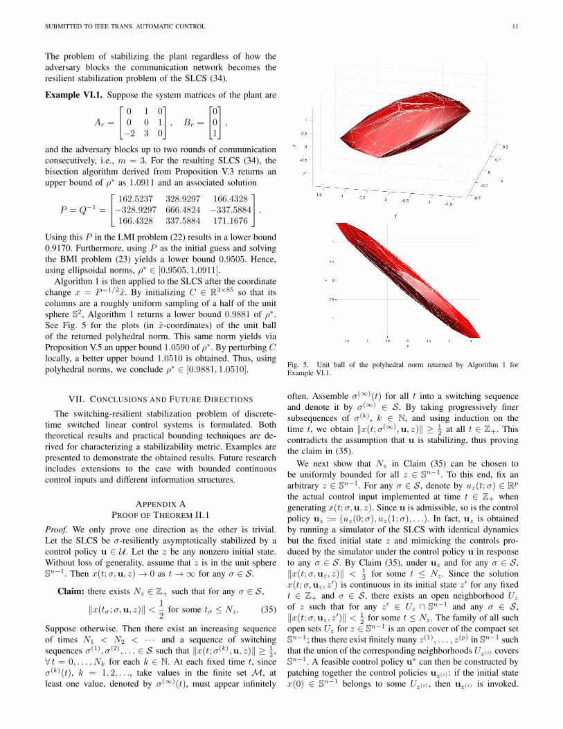
Ar =

0 1 00 0 1−2 3 0

, Br =

001

,and the adversary blocks up to two rounds of communicationconsecutively, i.e., m = 3. For the resulting SLCS (34), thebisection algorithm derived from Proposition V.3 returns anupper bound of ρ∗ as 1.0911 and an associated solution

P = Q−1 =

162.5237 328.9297 166.4328−328.9297 666.4824 −337.5884166.4328 337.5884 171.1676

.Using this P in the LMI problem (22) results in a lower bound0.9170. Furthermore, using P as the initial guess and solvingthe BMI problem (23) yields a lower bound 0.9505. Hence,using ellipsoidal norms, ρ∗ ∈ [0.9505, 1.0911].

Algorithm 1 is then applied to the SLCS after the coordinatechange x = P−1/2x. By initializing C ∈ R3×85 so that itscolumns are a roughly uniform sampling of a half of the unitsphere S2, Algorithm 1 returns a lower bound 0.9881 of ρ∗.See Fig. 5 for the plots (in x-coordinates) of the unit ballof the returned polyhedral norm. This same norm yields viaProposition V.5 an upper bound 1.0590 of ρ∗. By perturbing Clocally, a better upper bound 1.0510 is obtained. Thus, usingpolyhedral norms, we conclude ρ∗ ∈ [0.9881, 1.0510].

VII. CONCLUSIONS AND FUTURE DIRECTIONS

The switching-resilient stabilization problem of discrete-time switched linear control systems is formulated. Boththeoretical results and practical bounding techniques are de-rived for characterizing a stabilizability metric. Examples arepresented to demonstrate the obtained results. Future researchincludes extensions to the case with bounded continuouscontrol inputs and different information structures.

APPENDIX APROOF OF THEOREM II.1

Proof. We only prove one direction as the other is trivial.Let the SLCS be σ-resiliently asymptotically stabilized by acontrol policy u ∈ U . Let the z be any nonzero initial state.Without loss of generality, assume that z is in the unit sphereSn−1. Then x(t;σ,u, z)→ 0 as t→∞ for any σ ∈ S.

Claim: there exists Nz ∈ Z+ such that for any σ ∈ S,

‖x(tσ;σ,u, z)‖ < 1

2for some tσ ≤ Nz . (35)

Suppose otherwise. Then there exist an increasing sequenceof times N1 < N2 < · · · and a sequence of switchingsequences σ(1), σ(2), . . . ∈ S such that ‖x(t;σ(k),u, z)‖ ≥ 1

2 ,∀ t = 0, . . . , Nk for each k ∈ N. At each fixed time t, sinceσ(k)(t), k = 1, 2, . . ., take values in the finite set M, atleast one value, denoted by σ(∞)(t), must appear infinitely

Fig. 5. Unit ball of the polyhedral norm returned by Algorithm 1 forExample VI.1.

often. Assemble σ(∞)(t) for all t into a switching sequenceand denote it by σ(∞) ∈ S . By taking progressively finersubsequences of σ(k), k ∈ N, and using induction on thetime t, we obtain ‖x(t;σ(∞),u, z)‖ ≥ 1

2 at all t ∈ Z+. Thiscontradicts the assumption that u is stabilizing, thus provingthe claim in (35).

We next show that Nz in Claim (35) can be chosen tobe uniformly bounded for all z ∈ Sn−1. To this end, fix anarbitrary z ∈ Sn−1. For any σ ∈ S, denote by uz(t;σ) ∈ Rpthe actual control input implemented at time t ∈ Z+ whengenerating x(t;σ,u, z). Since u is admissible, so is the controlpolicy uz := (uz(0;σ), uz(1;σ), . . .). In fact, uz is obtainedby running a simulator of the SLCS with identical dynamicsbut the fixed initial state z and mimicking the controls pro-duced by the simulator under the control policy u in responseto any σ ∈ S . By Claim (35), under uz and for any σ ∈ S ,‖x(t;σ,uz, z)‖ < 1

2 for some t ≤ Nz . Since the solutionx(t;σ,uz, z

′) is continuous in its initial state z′ for any fixedt ∈ Z+ and σ ∈ S , there exists an open neighborhood Uzof z such that for any z′ ∈ Uz ∩ Sn−1 and any σ ∈ S ,‖x(t;σ,uz, z

′)‖ < 12 for some t ≤ Nz . The family of all such

open sets Uz for z ∈ Sn−1 is an open cover of the compact setSn−1; thus there exist finitely many z(1), . . . , z(p) in Sn−1 suchthat the union of the corresponding neighborhoods Uz(i) coversSn−1. A feasible control policy u∗ can then be constructed bypatching together the control policies uz(i) : if the initial statex(0) ∈ Sn−1 belongs to some Uz(i) , then uz(i) is invoked.

SUBMITTED TO IEEE TRANS. AUTOMATIC CONTROL 12

Let Nmax := maxi=1,...,pNz(i) < ∞. Under this u∗, for anyz ∈ Sn−1 and any σ ∈ S, ‖x(t;σ,u∗, z)‖ < 1

2 for somet ≤ Nmax. By a homogeneous extension of u∗ from Sn−1 toRn \ 0, we conclude that ‖x(t;σ,u∗, z)‖ < 1

2‖z‖ for somet ≤ Nmax, ∀ z 6= 0, ∀σ ∈ S . By restarting u∗ whenever thisoccurs and using a standard argument (e.g., [37, Proposition2.1]), we obtain an admissible control policy that σ-resilientlyexponentially stabilizes the SLCS.

APPENDIX BPROOF OF THEOREM III.1

Proof. By suitably scaling the matrices Ai’s, we can assumewithout loss of generality that ρ∗ = 1.

We first show that W defined in (8) is control σ-invariant.For any z ∈ W , ζ(z) < ∞ implies that there exist apolicy u = (u0,u1, . . .) ∈ U and κz ∈ [0,∞) such that‖x(t;σ,u, z)‖ ≤ κz , ∀ t, ∀σ = (σ0, σ1, . . .) ∈ S . Letv = u0(z) and let σ0 = i be arbitrary. Then the solutionstarting from x(1) = Aiz + Biv under the control policyu+ := (u1,u2, . . .) satisfies ‖x(t;σ+,u+, x(1))‖ = ‖x(t +1;σ,u, z)‖ ≤ κz for all t and all σ+ := (σ1, σ2, . . .) ∈ S . Asa result, ζ(x(1)) ≤ κz <∞ and thus x(1) ∈ W . This provesthat W is control σ-invariant. As the SLCS is irreducible, Wis either 0 or Rn. We show by contradiction that the formeris impossible. Suppose W = 0. Then for any z ∈ Sn−1 andany u ∈ U , there exist some σ ∈ S and sz,u,σ ∈ Z+ suchthat ‖x(sz,u,σ;σ,u, z)‖ > 2. We claim that the times sz,u,σare uniformly bounded in z and u:

Claim: ∃N ∈ Z+ such that ∀u ∈ U , ∀ z ∈ Sn−1,‖x(t;σ,u, z)‖ > 2 for some σ ∈ S and t ≤ N .

(36)

Suppose Claim (36) fails. Then there exist a sequence (zk)in Sn−1, a sequence of control policies (uk) in U , and astrictly increasing sequence of times (sk) such that for anyσ ∈ S, ‖x(t;σ,uk, zk)‖ ≤ 2, ∀ t = 0, . . . , sk for eachk ∈ N. By passing to a subsequence if necessary, we assumethat (zk) converges to some z∗ ∈ Sn−1. We next constructa control policy u∗ under which ‖x(t;σ,u∗, z∗)‖ ≤ 2 forall t ∈ Z+ and all σ ∈ S . To this purpose, for each k,we denote by ukzk,σ(t) the actual control at time t producedby the control policy uk for the initial state zk in responseto an arbitrary switching sequence σ ∈ S . We assumewithout loss of generality that ukzk,σ(t) lies in the orthogonalcomplement of ∩i∈MN (Bi) since the component of ukzk,σ(t)in ∩i∈MN (Bi) will not affect the state dynamics, where N (·)denotes the null space of a matrix. For any k and each t =0, . . . , sk−1, it follows from ‖x(t;σ,uk, zk)‖ ≤ 2 and ‖x(t+1;σ,uk, zk)‖ = ‖Aσ(t)x(t;σ,uk, zk) + Bσ(t)u

kzk,σ

(t)‖ ≤ 2,∀σ(t) ∈M that maxi∈M ‖Biukzk,σ(t)‖ ≤ 2

(maxi∈M ‖Ai‖+

1), which in turn implies that ukzk,σ(t) is uniformly boundedin (∩i∈MN (Bi))

⊥. Thus, for each fixed σ ∈ S and t ∈ Z+,(ukzk,σ(t)

)has a convergent subsequence whose limit is de-

noted by u∗z∗,σ(t). Let u∗ be the control policy that producesthe actual control u∗z∗,σ(t) at time t for the initial state z∗in response to any σ ∈ S , which is feasible since it is thelimit of a sequence of feasible control policies (uk). By thecontinuity of the state solution in initial state and control input

for each fixed σ, we deduce that ‖x(t;σ,u∗, z∗)‖ ≤ 2 for allt ∈ Z+ and all σ ∈ S . It follows from ρ∗ = 1 that ζ(z∗) ≤ 2and hence z∗ ∈ W , a contradiction to W = 0. This provesClaim (36).

Claim (36) then implies that, regardless of x(0) and u, therealways exists a switching sequence of length no more than Nunder which the state norm is at least doubled. Repeating thisswitching strategy by the adversary, we conclude that ρ∗ > 1,which contradicts the assumption ρ∗ = 1. Therefore, W 6=0. This implies W = Rn, i.e., ζ(·) is finite everywhere onRn. Thus ζ(·) is a norm on Rn, and ζ(·) ≤ κ‖ · ‖ for someconstant κ > 0. This shows that the SLCS is nondefective.

APPENDIX CPROOF OF THEOREM IV.1

Proof. The “only if” part has been proved; we prove the “if”part as follows. Suppose the SLCS is nondefective with ρ∗ >0. Then ζ(·) defined in (7) is finite everywhere and is thusa norm on Rn. Given u ∈ U and σ ∈ S, let (u0,u+) be adecomposition of u and (σ(0), σ+) a decomposition of σ. Foreach z ∈ Rn, we can rewrite

ζ(z) = infu0

infu+

supσ(0)

supσ+

supt∈Z+

‖x(t;σ,u, z)‖(ρ∗)t

= infu0

supσ(0)

infu+

supσ+

supt∈Z+

‖x(t;σ,u, z)‖(ρ∗)t

.

The reason that supσ(0) and infu+can switch order is due to

the observation in Remark II.1: for the objective of maximizingsupt∈Z+

‖x(t)‖/(ρ∗)t, knowing the optimal state feedbackcontrol policy u+ after time 0 gives no extra advantage to theadversary for its decision on σ(0). By denoting u0(z) = v andσ(0) = i, and using x(t + 1;σ,u, z) = x(t;σ+,u+, xi,v(1))where xi,v(1) := Aiz +Biv, we have, for any z ∈ Rn,

ζ(z)

= infv

supi

infu+

supσ+

max

(‖z‖, sup

t∈Z+

‖x(t;σ+,u+, xi,v(1))‖(ρ∗)t+1

)= inf

vsupi

max(‖z‖, ζ(Aiz +Biv)/ρ∗

)= max

(‖z‖, ζ](z)/ρ∗

).

It follows then that ζ(·) ≥ ζ](·)/ρ∗, i.e., ζ](·) ≤ ρ∗ · ζ(·),making ζ(·) an extremal norm of the SLCS.

Finally, if the SLCS is nondefective with ρ∗ = 0, then forany z ∈ Rn, there exists v ∈ Rp such that Aiz+Biv = 0,∀ i ∈M. This means that any norm ‖·‖ on Rn is an extremal normsince ‖ · ‖] ≡ 0.

APPENDIX DPROOF OF THEOREM IV.2

Proof. Suppose the SLCS is nondefective and ρ∗ > 0. Let‖·‖ be an arbitrary norm on Rn, and use T in (15) to define asequence of seminorms on Rn as ξ(0)(·) := ‖·‖, and ξ(t)(·) :=T · · · T︸ ︷︷ ︸

t times

(‖ · ‖) for each t ∈ N. By induction,

ξ(t)(z) = infu∈U

supσ∈S‖x(t;σ,u, z)‖, ∀ z ∈ Rn, t ∈ N. (37)

SUBMITTED TO IEEE TRANS. AUTOMATIC CONTROL 13

Therefore, ξ(t)(z)/(ρ∗)t ≤ ζ(z), ∀ t ∈ N, ∀ z ∈ Rn, whereζ is defined in (7). Since the SLCS is nondefective, ζ ispointwise finite on Rn; thus for each s ∈ N, supt≥s ξ

(t)/(ρ∗)t

is pointwise finite (and easily seen to be a seminorm) on Rn.Consider the following function defined for z ∈ Rn:

η(z) := lim supt→∞

ξ(t)(z)

(ρ∗)t= infs∈N

(supt≥s

ξ(t)(z)

(ρ∗)t

). (38)

Clearly, η ≤ ζ. Being the limit of a nonincreasing sequenceof seminorms supt≥s ξ

(t)/(ρ∗)t as s → ∞, η is a seminormon Rn. We next show that η 6≡ 0. Suppose otherwise. Thenfor any z ∈ Sn−1, we have limt→∞ ξ(t)(z)/(ρ∗)t → 0.By (37), there exist Nz ∈ N and uz ∈ U such that forany σ ∈ S , ‖x(t;σ,uz, z)‖ < 1

2 (ρ∗)t for some t ≤ Nz .Similar to the proof of Theorem II.1, we can first modifyuz in an open neighborhood Uz of z in Sn−1 to obtaina policy uz so that for any z′ ∈ Uz and any σ ∈ S,‖x(t;σ, uz, z

′)‖ < 12 (ρ∗)t for some t ≤ Nz; obtain finitely

many such Uz’s to cover Sn−1; patch their corresponding uztogether to form an overall control policy u ∈ U and a finiteuniform time bound Nmax such that for any z ∈ Sn−1 andany σ ∈ S, ‖x(t;σ, u, z)‖ < 1

2 (ρ∗)t for some t ≤ Nmax.Repeating this argument via induction, we deduce that the σ-resilient stabilizing rate is strictly less than ρ∗, a contradiction.Hence η is a nonzero seminorm on Rn. By applying T toboth sides of (38) and using the monotone continuity propertyestablished in Lemma IV.3, we have

η] = infs∈NT[supt≥s

ξ(t)

(ρ∗)t

]≥ inf

s∈N

(supt≥s

ξ(t)]

(ρ∗)t

)

= infs∈N

(supt≥s

ξ(t+1)

(ρ∗)t

)= ρ∗ · inf

s∈N

(supt≥s+1

ξ(t)

(ρ∗)t

)= ρ∗ · η,

where the second step follows from Lemma IV.3. Therefore,η is a lower extremal seminorm of the SLCS.

When the SLCS is nondefective with ρ∗ = 0, it is easilyverified that any seminorm ξ on Rn satisfies ξ] ≡ 0 and thusis a lower extremal seminorm.

APPENDIX EPROOF OF THEOREM IV.3

Proof. Suppose that the SLCS is irreducible with ρ∗ > 0.By Theorem III.1, the SLCS is also nondefective; thus thefunction ζ defined in (7) is pointwise finite on Rn. Define

χ(z) := infu∈U

supσ∈S

lim supt→∞

‖x(t;σ,u, z)‖(ρ∗)t

, ∀ z ∈ Rn.

Obviously, χ ≤ ζ. Hence χ is pointwise finite on Rn. Further,it is easy to see that χ is convex and positively homogeneouson Rn. Therefore, χ is a seminorm on Rn, whose kernelNχ := z |χ(z) = 0 is a subspace of Rn. Note thatχ(z + z′) = χ(z) for all z ∈ Rn and all z′ ∈ Nχ.

We claim that Nχ is control σ-invariant. Fix an ar-bitrary z ∈ Nχ. For any ε > 0, there exists acontrol policy uε = (uε0,u

ε1, . . .) ∈ U such that

lim supt→∞ ‖x(t;σ,uε, z)‖/(ρ∗)t < ε, ∀σ ∈ S. Let vε :=uε0(z) be the control input at t = 0 specified by uε and

let σ(0) = i ∈ M be arbitrary. Then the solution start-ing from x(1) := Aiz + Biv

ε under uε+ := (uε1,uε2, . . .)

satisfies x(t;σ+,uε+, x(1)) = x(t + 1;σ,uε, z) and hence

lim supt→∞ ‖x(t;σ+,uε+, x(1))‖/(ρ∗)t ≤ ρ∗ ·ε, for all σ+ :=

(σ(1), σ(2), . . .) ∈ S. This shows that χ(Aiz+Bivε) ≤ ρ∗ · ε

for all i ∈ M. Let εk > 0, k ∈ N, be such that εk ↓ 0, andlet vk := vεk for each k, which satisfies

χ(Aiz +Bivk) ≤ ρ∗ · εk, ∀ i ∈M. (39)

Define the subspace V := v |χ(Biv) = 0, ∀ i ∈ M ⊂Rp, and denote by V⊥ its orthogonal complement. Let v′kbe the projection of vk onto V⊥ for each k. Using (39) andthe argument in the proof of Lemma IV.2, we conclude thatthe sequence (v′k) is bounded. Hence a subsequence of (v′k)converges to some v∗ ∈ V⊥. Taking the limit of (39) for thissubsequence with vk replaced by v′k which does not changethe value of χ(·), we obtain via the continuity of the seminormχ(·) that χ(Aiz + Biv∗) = 0 for all i ∈ M. This shows thatNχ is a control σ-invariant subspace.

As the SLCS is irreducible, Nχ is either 0 or Rn. Werule out the latter via contradiction. Suppose χ ≡ 0 onRn. Consider the scaled SLCS (Ai/ρ∗, Bi/ρ∗)i∈M whosesolutions x(t;σ,u, z) = x(t;σ,u, z)/(ρ∗)t. Fix an arbitraryz ∈ Sn−1. For any ε > 0, there exists uz ∈ U such that for anyσ ∈ S , there exists tz,σ ∈ Z+ such that ‖x(t;σ,uz, z)‖ < εfor all t ≥ tz,σ . Following the argument in the proof of Claim(35) in Theorem II.1, we conclude that there exists a uniformTz ∈ Z+ such that for any σ ∈ S, ‖x(t;σ,uz, z)‖ < εfor some t ≤ Tz . By setting ε = 1/2 and using a similarargument as in Theorem II.1, we deduce that the scaledSLCS is σ-resiliently exponentially stabilizable. Hence its σ-resilient stabilizing rate ρ∗ < 1. By Lemma II.1, the σ-resilientstabilizing rate of the original SLCS is ρ∗ · ρ∗ which is strictlyless than ρ∗, a contradiction. This shows that Nχ = 0, i.e.,χ is a norm on Rn.

To show χ] = ρ∗ · χ, let z ∈ Rn be arbitrary. Decomposeu ∈ U and σ ∈ S as u = (u0,u+) and σ = (σ(0), σ+) asbefore. Denote v := u0(z) and i := σ(0). Then

χ(z) = infu0

supσ(0)

infu+

supσ+

lim supt→∞

‖x(t;σ,u, z)‖(ρ∗)t

= infv∈Rp

supi∈M

infu+

supσ+

lim supt→∞

‖x(t;σ+,u+, Aiz +Biv)‖(ρ∗)t+1

= infv∈Rp

supi∈M

χ(Aiz +Biv)

ρ∗=

χ](z)

ρ∗.

Again, in deriving the first equality we use the observation inRemark II.1 to exchange the order of infu+

and supσ(0). Asa result, χ] = ρ∗ · χ, proving that χ is a Barabanov norm.

If an irreducible SLCS has ρ∗ = 0, then any norm ‖ · ‖satisfies ‖ · ‖] = 0 and is a Barabanov norm.

REFERENCES

[1] R. DeCarlo, M. Branicky, S. Pettersson, and B. Lennartson, “Perspec-tives and results on the stability and stabilizability of hybrid systems,”Proceedings of the IEEE, vol. 88, no. 7, pp. 1069–1082, 2000.

[2] J. C. Geromel and P. Colaneri, “Stability and stabilization of discretetime switched systems,” International Journal of Control, vol. 79, no. 7,pp. 719–728, 2006.

SUBMITTED TO IEEE TRANS. AUTOMATIC CONTROL 14

[3] T. Hu, L. Ma, and Z. Lin, “Stabilization of switched systems via com-posite quadratic functions,” IEEE Transactions on Automatic Control,vol. 53, no. 11, pp. 2571–2585, 2008.

[4] H. Lin and P. J. Antsaklis, “Hybrid state feedback stabilization withl2 performance for discrete-time switched linear systems,” InternationalJournal of Control, vol. 81, no. 7, pp. 1114–1124, 2008.

[5] S. Pettersson and B. Lennartson, “Stabilization of hybrid systems usinga min-projection strategy,” in Proc. American Control Conference, 2001,pp. 223–228.

[6] W. Zhang, A. Abate, J. Hu, and M. P. Vitus, “Exponential stabilizationof discrete-time switched linear systems,” Automatica, vol. 45, no. 11,pp. 2526–2536, 2009, (Purdue Technical Report TR-ECE 09-01).

[7] Z. Ji, L. Wang, and G. Xie, “Quadratic stabilization of switchedsystems,” International Journal of Systems Science, vol. 36, no. 7, pp.395–404, 2005.

[8] L. Allerhand and U. Shaked, “Robust stability and stabilization of linearswitched systems with dwell time,” IEEE Transactions on AutomaticControl, vol. 56, no. 2, pp. 381–386, 2011.

[9] D. Cheng, L. Guo, Y. Lin, and Y. Wang, “Stabilization of switched linearsystems,” IEEE Transactions on Automatic Control, vol. 50, no. 5, pp.661–666, 2005.

[10] L. Fang, H. Lin, and P. J. Antsaklis, “Stabilization and performanceanalysis for a class of switched systems,” in 43rd IEEE Conference onDecision and Control, 2004, pp. 3265–3270.

[11] L. Hetel, J. Daafouz, and C. Iung, “Stabilization of arbitrary switchedlinear systems with unknown time-varying delays,” IEEE Transactionson Automatic Control, vol. 51, no. 10, pp. 1668–1674, 2006.

[12] M. Philippe, R. Essick, G. E. Dullerud, R. M. Jungers et al., “Theminimum achievable stability radius of switched linear systems withfeedback,” in Proc. IEEE Int. Conf. Decision and Control, 2015.

[13] G. Xie and L. Wang, “Stabilization of switched linear systems withtime-delay in detection of switching signal,” Journal of MathematicalAnalysis and Applications, vol. 305, no. 1, pp. 277–290, 2005.

[14] L. Zhang and P. Shi, “Stability, `2-gain and asynchronous control ofdiscrete-time switched systems with average dwell time,” IEEE Trans.Automat. Contr., vol. 54, no. 9, pp. 2192–2199, 2009.

[15] X. Zhao, L. Zhang, P. Shi, and M. Liu, “Stability and stabilization ofswitched linear systems with mode-dependent average dwell time,” IEEETrans. Automat. Contr., vol. 57, no. 7, pp. 1809–1815, 2012.

[16] M. Yu, L. Wang, G. Xie, and T. Chu, “Stabilization of networked controlsystems with data packet dropout and network delays via switchingsystem approach,” in 43rd IEEE Int. Conf. Decision and Control, 2004,pp. 3539–3544.

[17] A. Cardenas, S. Amin, and S. Sastry, “Secure control: Towards surviv-able cyber-physical systems.” in First International Workshop on Cyber-Physical Systems (WCPS2008), June 2008.

[18] M. C. de Oliveira, J. Bernussou, and J. C. Geromel, “A new discrete-time robust stability condition,” Systems and Control Letters, vol. 37,no. 4, pp. 261–265, 1999.

[19] P. P. Khargonekar, I. R. Petersen, and K. Zhou, “Robust stabilizationof uncertain linear systems: quadratic stabilizability and H∞ controltheory,” IEEE Trans. Automat. Contr., vol. 35, no. 3, pp. 356–361, 1990.

[20] M. V. Kothare, V. Balakrishnan, and M. Morari, “Robust constrainedmodel predictive control using linear matrix inequalities,” Automatica,vol. 32, no. 10, pp. 1361–1379, 1996.

[21] W.-J. Mao, “Robust stabilization of uncertain time-varying discretesystems and comments on an improved approach for constrained robustmodel predictive control,” Automatica, vol. 39, no. 6, pp. 1109–1112,2003.

[22] J. Stoustrup and V. D. Blondel, “Fault tolerant control: A simultaneousstabilization result,” IEEE Transactions on Automatic Control, vol. 49,no. 2, pp. 305–310, 2004.

[23] N. Barabanov, “Lyapunov indicators of discrete inclusions. I-III,” Au-tomation and Remote Control, vol. 49, pp. 152–157, 283–287, 558–565,1988.

[24] N. Guglielmi and M. Zennaro, “An algorithm for finding extremalpolytope norms of matrix families,” Linear Algebra and its Applications,vol. 428, no. 10, pp. 2265–2282, 2008.

[25] R. Jungers, The Joint Spectral Radius: Theory and Applications.Springer Science & Business Media, 2009, vol. 385.

[26] V. S. Kozyakin, “Algebraic unsolvability of problem of absolute stabilityof desynchronized systems,” Autom. Rem. Control, vol. 51, no. 6, pp.754–759, 1990.

[27] E. Plischke, F. Wirth, and N. Barabanov, “Duality results for the jointspectral radius and transient behavior,” in 44th IEEE Int. Conf. Decisionand Control, 2005, pp. 2344–2349.

[28] G.-C. Rota and G. Strang, “A note on the joint spectral radius,”Proceedings of the Netherlands Academy, vol. Ser. A 63, no. 22, pp.379–381, 1960.

[29] S. Boyd and L. Vandenberghe, Convex Optimization. CambridgeUniversity Press, 2004.

[30] N. Guglielmi and M. Zennaro, “On the asymptotic properties of a familyof matrices,” Linear Algebra and its Applications, vol. 322, no. 1, pp.169–192, 2001.

[31] W. Rudin, Functional Analysis. McGraw-Hill, 1979.[32] F. Wirth, “The generalized spectral radius and extremal norms,” Linear

Algebra and its Applications, vol. 342, no. 1, pp. 17–40, 2002.[33] M. Margaliot, “Stability analysis of switched systems using variational

principles: An introduction,” Automatica, vol. 42, no. 12, pp. 2059–2077,2006.

[34] K. Ball, “An elementary introduction to modern convex geometry,”Flavors of Geometry, vol. 31, pp. 1–58, 1997.

[35] F. John, “Extremum problems with inequalities as subsidiary condi-tions,” in Studies and Essays presented to R. Courant on His 60thBirthday. New York: Interscience, Jan. 1948, pp. 187–204.

[36] S. Boyd, L. El Ghaoui, E. Feron, and V. Balakrishnan, Linear MatrixInequalities in System and Control Theory. SIAM, 1994, vol. 15.

[37] J. Shen and J. Hu, “Stability of discrete-time switched homogeneoussystems on cones and conewise homogeneous inclusions,” SIAM J.Control and Optimization, vol. 50, no. 4, pp. 2216–2253, 2012.

Jianghai Hu Jianghai Hu (S’99-M’04) receivedthe B.E. degree in automatic control from Xi’anJiaotong University, P.R. China, in 1994, and theM.A. degree in Mathematics and the Ph.D. degreein Electrical Engineering from the University ofCalifornia, Berkeley, in 2002 and 2003, respectively.He is currently an Associate Professor with theSchool of Electrical and Computer Engineering, Pur-due University. His research interests include hybridsystems, multi-agent systems, control of systemswith uncertainty, and control applications. He is an

Associate Editor of SIAM Journal on Control and Optimization and NonlinearAnalysis: Hybrid Systems. He currently serves as the IEEE Control SystemSociety Electronic Publications Editor.

Jinglai Shen (S’01-A’03-M’05-SM’10) Jinglai Shenreceived the B.S.E. and M.S.E. degrees in automaticcontrol from Beijing University of Aeronautics andAstronautics, China, in 1994 and 1997, respectively,and the Ph.D. degree in aerospace engineering fromthe University of Michigan, Ann Arbor, in 2002. Heis currently an Associate Professor at the Departmentof Mathematics and Statistics, University of Mary-land Baltimore County (UMBC). Before joiningUMBC, he was a Postdoctoral Research Associate atRensselaer Polytechnic Institute, Troy, NY. His re-

search interests include nonsmooth hybrid and switching systems, continuousoptimization and optimal control, constrained estimation, multibody dynamicsand nonlinear control with applications to engineering and statistics. He is anAssociate Editor of SIAM Journal on Control and Optimization.

Donghwan Lee (S’13) Donghwan Lee received theB.S. degree in Electronic Engineering from KonkukUniversity, Seoul, Korea, in 2008 and M.S. degreein the School Electrical and Electronic Engineeringfrom Yonsei University, Seoul, Korea, in 2010. Cur-rently, he is working toward a Ph.D. degree in theDepartment of Electrical and Computer Engineering,Purdue University. His current research interestsinclude stability and stabilization of switched linearsystems.