Submarine Slope Stability - Bureau of Safety and ...
269
Submarine Slope Stability Based on M.S. Engineering Thesis Development of a Database and Assessment of Seafloor Slope Stability Based on Published Literature By James Johnathan Hance, B. S. The University of Texas at Austin Supervisor Dr. Stephen G. Wright The University of Texas at Austin Project Report Prepared for the Minerals Management Service Under the MMS/OTRC Cooperative Research Agreement 1435-01-99-CA-31003 Task Order 18217 MMS Project 421 August 2003
Transcript of Submarine Slope Stability - Bureau of Safety and ...
Submarine Slope Stability
Based on M.S. Engineering Thesis
Development of a Database and Assessment of Seafloor Slope Stability Based on Published Literature
By
James Johnathan Hance, B. S. The University of Texas at Austin
Supervisor
Dr. Stephen G. Wright
The University of Texas at Austin
Project Report Prepared for the Minerals Management Service Under the MMS/OTRC Cooperative Research Agreement
1435-01-99-CA-31003 Task Order 18217 MMS Project 421
August 2003

OTRC Library Number: 8/03B121
Fo
Offshor
Colle
Offshor
The 1A
A National Science
r more information contact:
e Technology Research Center
Texas A&M University 1200 Mariner Drive
ge Station, Texas 77845-3400 (979) 845-6000
or
e Technology Research Center
University of Texas at Austin University Station C3700 ustin, Texas 78712-0318
(512) 471-6989
Foundation Graduated Engineering Research Center
Submarine Slope Stability
Executive Summary Background and Context Oil and gas developments often require placing equipment, e.g., subsea wells, pipelines and flowlines, foundation systems for floating structures, in areas with sloping seafloors. Submarine slope failures can occur in such areas and create soil slides. Thus the stability of submarine slopes must be considered in selecting the site for installing and designing seafloor equipment. Assessing submarine slope stability requires estimating the likelihood, extent, and impact of a slide during the lifetime of the facility. This assessment is difficult due to the large difference in time scales between the project life (10’s of years) and the geologic processes and triggering mechanisms that cause the slides (10,000’s of years) Such an assessment is best approached through a probabilistic risk analysis that considers the risks to the equipment; the causes, likelihood, and behavior of submarine slides; and the uncertainties. A forum of experts from industry, government, and academia was held in 2002 (1, 2) to discuss the current state-of-the-art and state-of-the-practice and to identify areas where future research was needed to advance capabilities to assess submarine slope stability and the impact of submarine slides. That forum concluded that a comprehensive data base should be developed for historical slides containing information on the seafloor characteristics (soil properties, slope topography, geology), triggering mechanisms, and the characteristics and extent of the slide. This database could then be used to develop, improve, and test models for predicting slope stability, slide occurrence and behavior, and to assess the impact of uncertainties in seafloor characteristics and triggering mechanisms in predicting the likelihood and behavior of slides. By looking for similarities between a new site under investigation for a subsea installation and sites of historical slides, data from the historical slides might also be useful in assessing the slope stability and risks of a slide for the new site. This was the basis for the project reported here. Development of a Database and Assessment of Seafloor Slope Stability based on Published Literature This work resulted from a research project conducted by J.J. Hance for his Master of Science in Engineering at the University of Texas under the supervision of Dr. Stephen G. Wright. Hance’s thesis (3) is attached Based on published literature, a database was compiled the includes 534 submarine slide events. The database contains information on the geographic location, water depth, date and type of failure, potential triggering mechanisms, dimensions, slope angle, and soil types and properties. The data were examined to identify important characteristics of seafloor slope failures. While the database is substantial, significant geotechnical information was not available for many slope failures. Fourteen different triggering mechanisms were identified and included in the database. Earthquakes are the most commonly reported trigger.
Slope stability analyses were performed to assess the likelihood of slides being triggered by gravity, rapid sedimentation (underconsolidation) and earthquakes. The analyses revealed that it is unlikely that most of the seafloor slope failures were triggered by gravity loads alone. Earthquake loading was confirmed as a common trigger, and rapid sedimentation (underconsolidation) was also a likely trigger of many slope failures. It is important to note that the study revealed that a relatively large number of submarine slides occurred on much flatter (less than 10 degree) slopes and traveled much greater distances than slope failures on land. This strongly suggests that different mechanisms are prevalent for submarine slides, compared to those on land. Hydroplaning is one mechanism that may explain such large runout distances. The mechanism of hydroplaning is summarized, and a simple sliding block model is presented to illustrate how conditions for hydroplaning can be developed. Rheological models have also been developed to explain slide runout, and several models are described. However, the rheological models do not seem to explain some of the very large runout distances observed in both experiments and actual seafloor slides. For many slides, hydroplaning appears to be the mechanism that can best account for large runout distances. References Wright, Stephen G., "Forum on Risk Assessment for Submarine Slope Stability - Report of a Forum Held In Houston, Texas - May 10 And 11, 2002", June, 2002 (Offshore Technology Research Center Report). Wright, Stephen G., Gilbert, Robert B., and Smith, Charles E., "Risk Assessment of Submarine Slope Stability in Deepwater - Issues and Priorities", Proceedings, 14th Deep Offshore Technology Conference, New Orleans, Louisiana, November 13-15, 2003. Hance, J.J. (2003). “Development of a database and assessment of seafloor slope stability based on published literature.” M.S. Thesis, University of Texas at Austin.

Development of a Database and
Assessment of Seafloor Slope
Stability based on Published Literature
by
James Johnathan Hance, B.S.
Thesis
Presented to the Faculty of the Graduate School
of The University of Texas at Austin
in Partial Fulfillment
of the Requirements
for the Degree of
Master of Science in Engineering
The University of Texas at Austin
August 2003
Development of a Database and
Assessment of Seafloor Slope
Stability based on Published Literature
APPROVED BY
SUPERVISING COMMITTEE:
Stephen G. Wright Robert B. Gilbert

Copyright
by
James Johnathan Hance
2003
ACKNOWLEDGEMENTS
There are several people I must thank for their efforts and encouragement
during the preparation of this thesis. Without their positive involvement in this
process, this thesis would not have been completed. First, I am grateful for the
opportunity to work with my primary supervisor, Dr. Stephen G. Wright. His
continued interest and involvement in the development of this project has been
rewarding. He has offered guidance in maintaining a proper direction for this
thesis while ensuring that the research process has been educational for me as a
young engineer. I am thankful that Dr. Robert Gilbert became involved in this
project. He was efficient in reviewing the manuscript and results from the
database. I also thank Dr. Ellen Rathje who helped me with the part of my thesis
that involved evaluating seismicity and pseudo-static slope stability.
I am grateful for the financial support provided by the Offshore
Technology and Research Center (OTRC) during my involvement with this
project. I thank the people on the 9th floor who always had a smile on their face,
namely Teresa Tice-Boggs, Chris Treviño, Alicia Zapata, and Dr. Roy Olson. A
special thanks also goes out to the friends I have made within the Geotechnical
Engineering Program.
iv

My parents, James Hance and Brenda Ruffner, have always been a driving
force in my life, and I am thankful for their encouragement during my graduate
studies at The University of Texas at Austin. I would also like to thank my
stepparents, Gary Ruffner and Joan Hance, and my younger brothers, Matt, Pat
and Harry.
Finally, I must acknowledge the daily support and love provided by my
wonderful fiancée, Jennifer Graves. She has helped me whenever necessary, and
I am forever indebted to her.
v
Development of a Database and
Assessment of Seafloor Slope
Stability based on Published Literature
by
James Johnathan Hance, M.S.E.
The University of Texas at Austin, 2003
SUPERVISOR: Stephen G. Wright
A database of seafloor slope failures has been created from the published
literature. The database contains information on the geographic location, date and
type of failure, potential triggering mechanisms, soil types, soil properties,
dimensions, slope angle, and water depths for the slope failures. Data in the
database have been examined to identify important characteristics of seafloor
slope failures. However, while there is substantial information in the database,
significant geotechnical information was lacking for many of the slope failures.
Fourteen different triggering mechanisms have been identified and are
included in the database. Each of these triggers is discussed. The most common
trigger reported is earthquake loading.
vi
Seafloor slope failures (slides) can affect large areas and volumes of soil,
and they tend to be larger than subaerial landslides. Also, in comparison to
subaerial landslides, seafloor slides tend to travel larger distances and occur on
flatter slopes.
Slope stability analyses were performed and results are presented to assess
the likelihood of slides being triggered by gravity, rapid sedimentation
(underconsolidation) and earthquakes. The analyses reveal that it is unlikely that
most seafloor slope failures are triggered by gravity loads alone; earthquake
loading and rapid sedimentation (underconsolidation) are likely triggers of many
slope failures.
Many seafloor slides are accompanied by very large runout distances.
Hydroplaning is one mechanism that may explain such large runout distances.
The mechanism of hydroplaning is summarized, and a simple sliding block model
is presented to illustrate how conditions for hydroplaning can be developed.
Rheological models have also been developed to explain slide runout, and several
models are described. However, the rheological models do not seem to explain
some of the very large runout distances observed in both experiments and for
actual seafloor slides. For many slides, hydroplaning appears to be the
mechanism that best accounts for large runout distances.
vii
TABLE OF CONTENTS
List of Tables .................................................................................................xii List of Figures................................................................................................xv Chapter 1 Introduction...................................................................................1 Chapter 2 Literature Review..........................................................................3 2.1 Introduction..................................................................................3 2.2 The Body of Literature ................................................................3 2.3 How Data was Collected from the Literature ..............................5 Chapter 3 Structure and Content of the Database..........................................6 3.1 Introduction..................................................................................6 3.2 Included and Excluded Information ............................................6 3.3 Structure and Content of the Database ........................................7 3.4 How the Database was Used........................................................19 Chapter 4 Triggering Mechanisms ................................................................21 4.1 Introduction..................................................................................21 4.2 Types of Triggering Mechanisms ................................................22 4.3 Summary......................................................................................57 Chapter 5 Evaluation of Characteristics of Slope Failures in the Database ..58 5.1 Introduction..................................................................................58 5.2 Characteristics of the Database Fields .........................................59
viii
5.3 Date of Slope Failures..................................................................62 5.4 Triggering Mechanisms ...............................................................66 5.5 Geographic Location of Slope Failures .......................................73 5.6 Geographic Distribution of Slope Failures for Various Triggering Mechanisms......................................77 5.7 Slope Angle..................................................................................89 5.8 Dimensions of Slope Failures ......................................................91 5.9 Water Depths ...............................................................................103 5.10 Soil Type....................................................................................106 5.11 Runout Characteristics of Subaqueous Slides Compared to Subaerial and Quick Clay Slides......................109 5.12 Conclusions................................................................................118 Chapter 6 Infinite Slope Stability Analyses and Correlations with Seismicity..............................................................................120 6.1 Introduction..................................................................................120 6.2 Analyses for Static Conditions ....................................................120 6.3 Analyses for Pseudo-Static Conditions........................................129 6.4 Correlation of Results from Pseudo-Static Analyses with Seismicity.......................................................133 6.5 Conclusions..................................................................................140 Chapter 7 Hydroplaning Mechanism.............................................................141 7.1 Introduction..................................................................................141
ix
7.2 Definition of Hydroplaning .........................................................141 7.3 Overview of Past Experiments ....................................................143 7.4 Mohrig et al.’s (1998, 1999) Experiments...................................145 7.5 Hypothesis of Hydroplaning of Seafloor Slides Based on Geophysical Imagery .............................................158 7.6 Densimetric Froude Number: Indicator of Hydroplaning based on Experimental Results ..................159 7.7 Densimetric Froude Numbers Calculated for Seafloor Slides .................................................................163 7.8 Slides from the Database that may have Hydroplaned ................166 7.9 Role of Soil Strength in Producing Required Velocities for Hydroplaning ..................................................167 7.10 Estimating Strength Losses Required for Hydroplaning to Occur ..........................................................170 7.11 Conclusions................................................................................176 Chapter 8 Rheological Models for Seafloor Slide Runout ............................178 8.1 Introduction..................................................................................178 8.2 Rheological Models .....................................................................179 8.3 Numerical Model .........................................................................187 8.4 Conclusions..................................................................................194 Chapter 9 Summary, Conclusions, and Recommendations...........................195 9.1 Summary and Conclusions ..........................................................195 9.2 Recommendations for Future Work ............................................198
x
Appendix A: User’s Guide for Database of Seafloor Slope Failures ............202 Bibliography ..................................................................................................212 Vita.................................................................................................................245
xi

LIST OF TABLES Table 3.1 Description of terms that appear in the landslide description field .....................................................................13 Table 4.1 Information Relevant to Earthquakes or Faulting as Triggering Mechanisms ..................................23 Table 4.2 Information Relevant to Sedimentation Processes as a Triggering Mechanism...................................28 Table 4.3 Information Relevant to Gas Related Triggering Mechanisms .........................................................37 Table 4.4 Frequency of storm systems according to latitude ........................39 Table 4.5 Information in the Database Relevant to Ocean Waves as a Potential Triggering Mechanism ....................................40 Table 4.6 Information Relevant to Tidal Events as a Triggering Mechanism....................................................41 Table 4.7 Information Relevant to Human Activity as a Triggering Mechanism....................................................42 Table 4.8 Information Pertinent to Erosion Processes as a Triggering Mechanism....................................................43 Table 4.9 Information Relevant to Magma Volcanic Activity as a Triggering Mechanism .....................................44 Table 4.10 Information Relevant to Salt Diapirism as a Triggering Mechanism....................................................50 Table 4.11 Information Relevant to Mud Volcanoes as a Triggering Mechanism....................................................53 Table 4.12 Information Pertinent to Flood Events as a Triggering Mechanism....................................................54
xii
Table 4.13 Information Relevant to Creep as a Triggering Mechanism...........................................................55 Table 4.14 Information Pertinent to Tsunamis as a Triggering Mechanism....................................................56 Table 4.15 Information Relevant to Sea-Level Fluctuations as a Triggering Mechanism...............................57 Table 5.1 Summary of data that is available in the fields of the database .......................................................................60 Table 5.2 Qualification of data regarding the 225 earthquake-triggered seafloor slope failures captured in the database.....................68 Table 5.3 Summary of characteristics of seafloor slope failures in the database........................................................................119 Table 6.1 Regression coefficients used to calculate PGAROCK .................................136 Table 6.2 Seismic conditions required to cause permanent deformation in a slope with ky = 0.13 g.................................138 Table 6.3 Case histories, where earthquakes are cited as a probable trigger, that include data for magnitude, distance and slope angle ........................................................139 Table 7.1 Experimental results of sandy silt slurry (Mohrig et al., 1998) .....153 Table 7.2 Experimental results of silty clay slurry (Mohrig et al., 1999)......153 Table 7.3 Calculated densimetric Froude numbers based on experimental measurements....................................161 Table 7.4 Calculations of fluid stagnation pressures and average debris normal pressures .........................................................163 Table 7.5 Submarine slide case histories with calculated densimetric Froude numbers..................................................165
xiii

Table 7.6 Inferred Velocities from submarine cable breaks and “critical” slide velocities for the five slides that hydroplaned ....................................................................169 Table 7.7 Soil conditions and triggering mechanisms of five seafloor slides believed to have hydroplaned ........................172 Table 8.1 Parameters for stress-strain rate relationship of bilinear fluid (Imran et al., 2001)...........................................186 Table 8.2 Input parameters from numerical simulations (Imran et al., 2001) ................................................................188 Table 8.3 Output from the numerical simulations (Imran et al., 2001) .........190 Table 8.4 Input parameters for Marr et al.’s (2002) simulations...................193 Table 8.5 Observed runout characteristics and output from Marr et al.’s (2002) simulations.............................................194
xiv
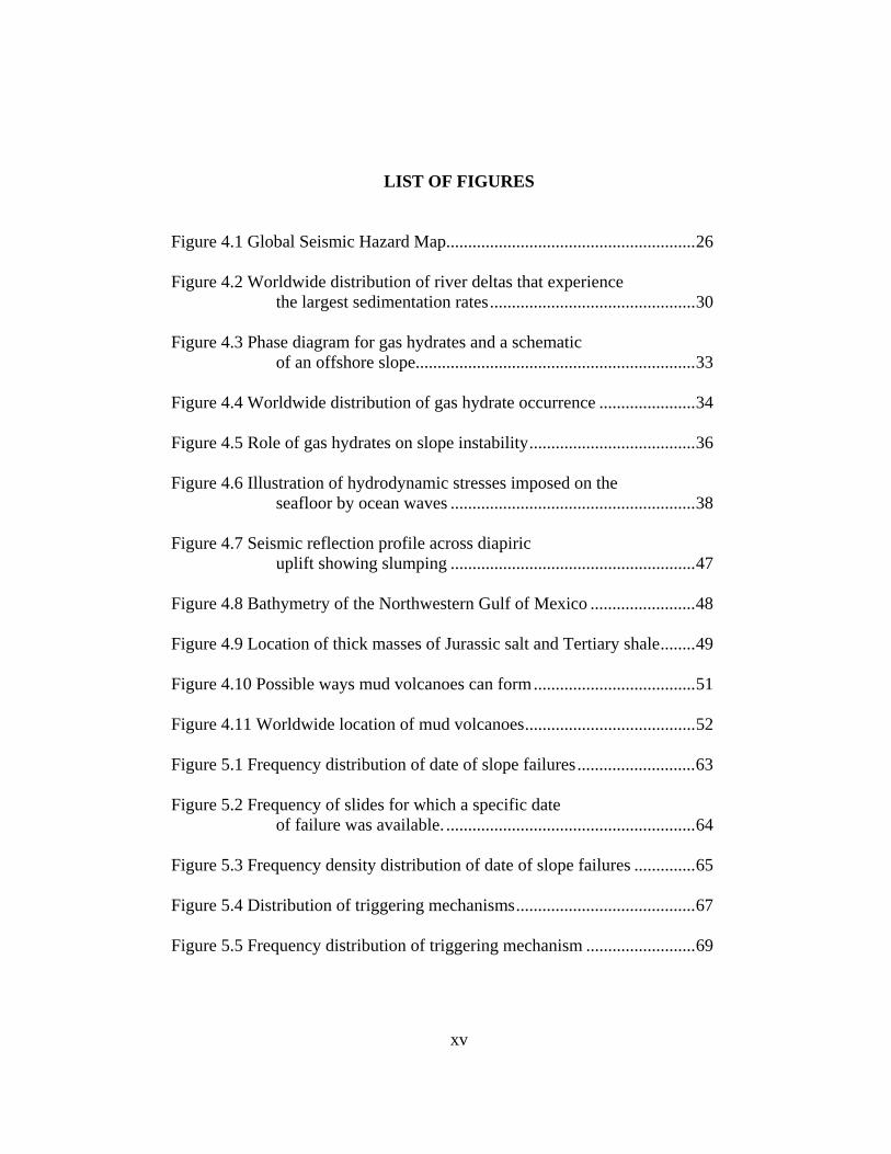
LIST OF FIGURES Figure 4.1 Global Seismic Hazard Map.........................................................26 Figure 4.2 Worldwide distribution of river deltas that experience the largest sedimentation rates...............................................30 Figure 4.3 Phase diagram for gas hydrates and a schematic of an offshore slope................................................................33 Figure 4.4 Worldwide distribution of gas hydrate occurrence ......................34 Figure 4.5 Role of gas hydrates on slope instability......................................36 Figure 4.6 Illustration of hydrodynamic stresses imposed on the seafloor by ocean waves ........................................................38 Figure 4.7 Seismic reflection profile across diapiric uplift showing slumping ........................................................47 Figure 4.8 Bathymetry of the Northwestern Gulf of Mexico ........................48 Figure 4.9 Location of thick masses of Jurassic salt and Tertiary shale........49 Figure 4.10 Possible ways mud volcanoes can form.....................................51 Figure 4.11 Worldwide location of mud volcanoes.......................................52 Figure 5.1 Frequency distribution of date of slope failures...........................63 Figure 5.2 Frequency of slides for which a specific date of failure was available. .........................................................64 Figure 5.3 Frequency density distribution of date of slope failures ..............65 Figure 5.4 Distribution of triggering mechanisms.........................................67 Figure 5.5 Frequency distribution of triggering mechanism .........................69
xv
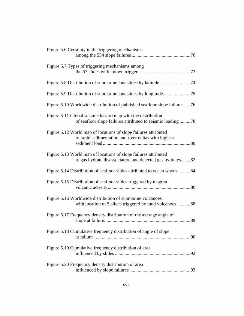
Figure 5.6 Certainty in the triggering mechanisms among the 534 slope failures .................................................70 Figure 5.7 Types of triggering mechanisms among the 57 slides with known triggers ..........................................72 Figure 5.8 Distribution of submarine landslides by latitude..........................74 Figure 5.9 Distribution of submarine landslides by longitude.......................75 Figure 5.10 Worldwide distribution of published seafloor slope failures .....76 Figure 5.11 Global seismic hazard map with the distribution of seafloor slope failures attributed to seismic loading .........78 Figure 5.12 World map of locations of slope failures attributed to rapid sedimentation and river deltas with highest sediment load .........................................................................80 Figure 5.13 World map of locations of slope failures attributed to gas hydrate disassociation and detected gas hydrates........82 Figure 5.14 Distribution of seafloor slides attributed to ocean waves...........84 Figure 5.15 Distribution of seafloor slides triggered by magma volcanic activity.....................................................................86 Figure 5.16 Worldwide distribution of submarine volcanoes with location of 5 slides triggered by mud volcanoes ...........88 Figure 5.17 Frequency density distribution of the average angle of slope at failure........................................................................89 Figure 5.18 Cumulative frequency distribution of angle of slope at failure .................................................................................90 Figure 5.19 Cumulative frequency distribution of area influenced by slides ...............................................................92 Figure 5.20 Frequency density distribution of area influenced by slope failures ...................................................93
xvi
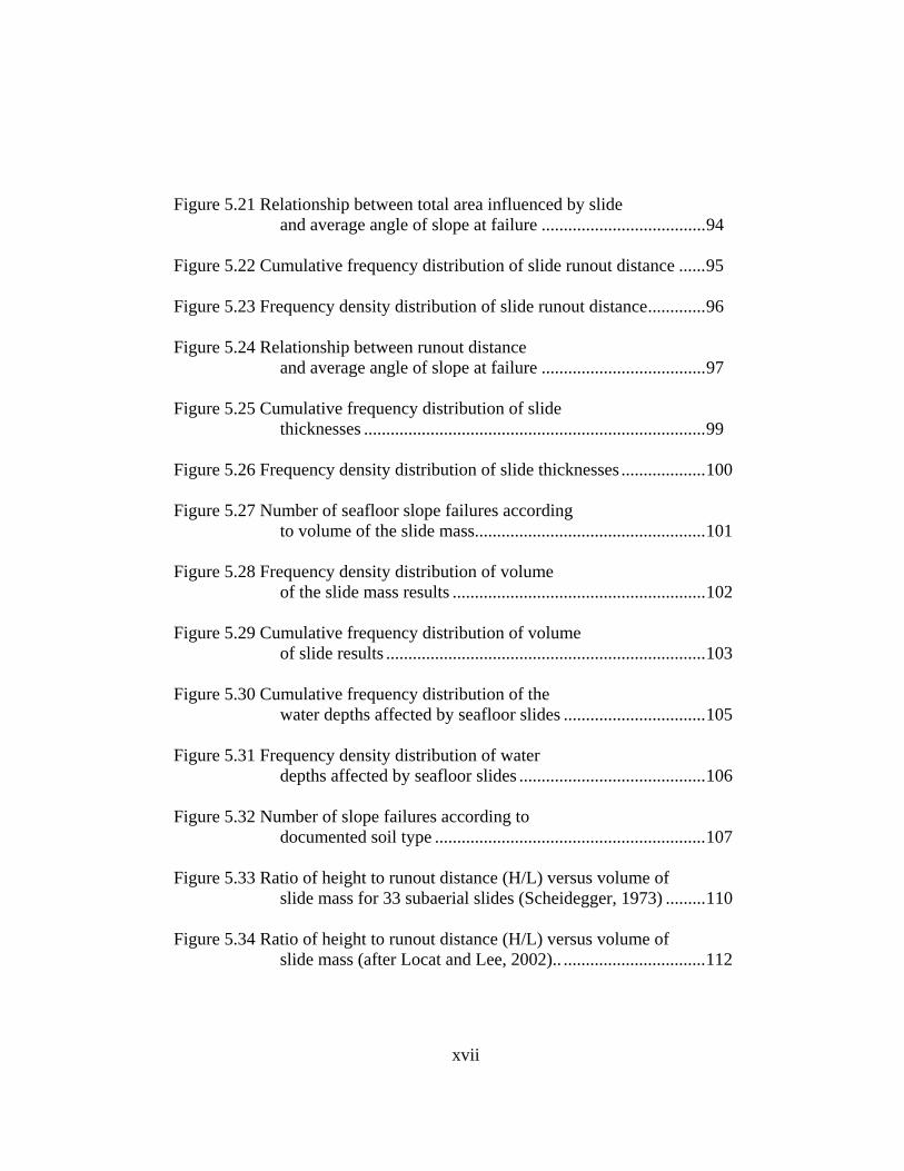
Figure 5.21 Relationship between total area influenced by slide and average angle of slope at failure .....................................94 Figure 5.22 Cumulative frequency distribution of slide runout distance ......95 Figure 5.23 Frequency density distribution of slide runout distance.............96 Figure 5.24 Relationship between runout distance and average angle of slope at failure .....................................97 Figure 5.25 Cumulative frequency distribution of slide thicknesses .............................................................................99 Figure 5.26 Frequency density distribution of slide thicknesses ...................100 Figure 5.27 Number of seafloor slope failures according to volume of the slide mass....................................................101 Figure 5.28 Frequency density distribution of volume of the slide mass results .........................................................102 Figure 5.29 Cumulative frequency distribution of volume of slide results ........................................................................103 Figure 5.30 Cumulative frequency distribution of the water depths affected by seafloor slides ................................105 Figure 5.31 Frequency density distribution of water depths affected by seafloor slides ..........................................106 Figure 5.32 Number of slope failures according to documented soil type .............................................................107 Figure 5.33 Ratio of height to runout distance (H/L) versus volume of slide mass for 33 subaerial slides (Scheidegger, 1973) .........110 Figure 5.34 Ratio of height to runout distance (H/L) versus volume of slide mass (after Locat and Lee, 2002).. ................................112
xvii
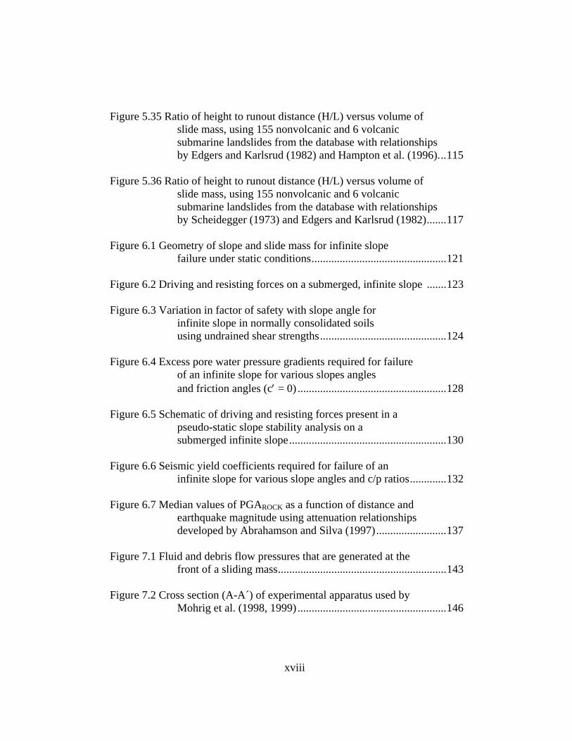
Figure 5.35 Ratio of height to runout distance (H/L) versus volume of slide mass, using 155 nonvolcanic and 6 volcanic submarine landslides from the database with relationships by Edgers and Karlsrud (1982) and Hampton et al. (1996)...115 Figure 5.36 Ratio of height to runout distance (H/L) versus volume of slide mass, using 155 nonvolcanic and 6 volcanic submarine landslides from the database with relationships by Scheidegger (1973) and Edgers and Karlsrud (1982).......117 Figure 6.1 Geometry of slope and slide mass for infinite slope failure under static conditions................................................121 Figure 6.2 Driving and resisting forces on a submerged, infinite slope .......123 Figure 6.3 Variation in factor of safety with slope angle for infinite slope in normally consolidated soils using undrained shear strengths.............................................124 Figure 6.4 Excess pore water pressure gradients required for failure of an infinite slope for various slopes angles and friction angles (c′ = 0) .....................................................128 Figure 6.5 Schematic of driving and resisting forces present in a pseudo-static slope stability analysis on a submerged infinite slope........................................................130 Figure 6.6 Seismic yield coefficients required for failure of an infinite slope for various slope angles and c/p ratios.............132 Figure 6.7 Median values of PGAROCK as a function of distance and earthquake magnitude using attenuation relationships developed by Abrahamson and Silva (1997).........................137 Figure 7.1 Fluid and debris flow pressures that are generated at the front of a sliding mass............................................................143 Figure 7.2 Cross section (A-A´) of experimental apparatus used by Mohrig et al. (1998, 1999) .....................................................146
xviii
Figure 7.3 Setup (profile view) for Mohrig et al.’s (1998, 1999) experiments (modified from Mohrig et al., 1998) .................147 Figure 7.4 Grain size distributions for soil used in Mohrig et al.’s (1998, 1999) experiments ......................................................149 Figure 7.5 Observed debris flow profiles from the experimental subaqueous runs ...............................................155 Figure 7.6 Velocities of the front of a slide versus downslope distance for the Mohrig et al. (1999) experiments...............................157 Figure 7.7 Interpretive three-dimensional image of the Kitimat Inlet landslide in British Columbia...........................159 Figure 7.8 Calculated densimetric Froude numbers versus runout distance based on six seafloor slide case histories.................166 Figure 7.9 Slides that may have hydroplaned considering the characteristics of runout distance (> 20 km) and slope angle (< 5 deg).......................................................168 Figure 7.10 Model of block sliding on an inclined plane used to examine what conditions might be required to achieve critical velocity and hydroplaning .........................................171 Figure 7.11 Velocity of a sliding block versus downslope movement in terms of shear strength loss after failure (β – φr)...............175 Figure 8.1 Stress-strain rate relationships......................................................181 Figure 8.2 Representation of viscoplastic model with a flowing soil mass on a slope ......................................................................182 Figure 8.3 Bilinear rheological model ...........................................................185 Figure 8.4 Stress-strain rate relationship for bilinear fluid model (after Imran et al., 2001) ........................................................186 Figure 8.5 Schematic of the geometry of the flow mass prior to movement down the inclined slope ...................................189
xix

Figure 8.6 Initial shape of debris flow for numerical simulations performed by Imran et al. (2001)...........................................189 Figure 8.7 Shapes of subaerial and subaqueous debris flows
(a) during downslope movement; (b) final shape at end of simulation (after Imran et al., 2001)..................................191
xx

CHAPTER 1
INTRODUCTION
Seafloor slope failures occur beneath many of the world’s oceans and
could impact all types of offshore and coastal facilities. In order to understand
better and assess the likelihood of seafloor slope failures, this study was
undertaken to compile and analyze data on such failures. Information that
pertains to evaluating the potential occurrence of a landslide, such as
characterizing the conditions in which landslides are known to take place, was
compiled. Due to the difficulties and costs in exploring the marine environment,
there is a high level of uncertainty in the stability of seafloor slopes. In an effort
to reduce this uncertainty, emphasis in this project was on compiling data and
creating a database of seafloor slope failures that have been reported in the
literature. Much of the effort for this project was directed to forming the
database.
Information related to seafloor landslides was examined in hundreds of
references including textbooks, reports, magazine articles, theses, dissertations,
Internet websites, maps, and technical papers from journals and conference
proceedings. Information from each reference that was considered to be pertinent
in describing a particular landslide event was extracted, and entered into fields in
a database. The database was created as a single table in Microsoft Access, with
1
the fields forming columns and the landslide entries forming rows. Once the
database was formed, the data were analyzed. Various types of information in the
database were evaluated, and results were summarized into tables and figures.
The review of the literature used to create the database is explained in
Chapter 2. Chapter 3 contains a description of the structure of the database and
the content of the fields (columns) in the database table. Causes of seafloor slope
failure, i.e. triggering mechanisms, are discussed in Chapter 4. Because the
triggering mechanisms are complex processes, a number of fields in the database
contain information pertaining to triggering mechanisms. The data are analyzed
and characteristics of seafloor slope failures are examined in Chapter 5. Results
of slope stability analyses performed to assess the likelihood of seafloor slides
being triggered by several triggering mechanisms are presented in Chapter 6.
Because some seafloor slides travel large distances, models that have been
developed to explain the large movements are of interest and are examined in
Chapters 7 and 8. An overview of the conclusions of this research program and
recommendations for future research are presented in Chapter 9.
2
CHAPTER 2
LITERATURE REVIEW
2. 1 INTRODUCTION
An extensive investigation of the literature was conducted to find as many
documented cases of seafloor slope failure as possible. The cases were then
summarized in tabular format into a database. The body of literature and the
methods used to collect the data are described in this chapter.
2.2 THE BODY OF LITERATURE
The literature investigated for this project was mainly comprised of
technical papers found in geological journals and periodicals. Some of the main
journals included Marine Geotechnology, Marine Geology, Geo-Marine Letters,
American Association of Petroleum Geologists Bulletin, and the USGS Survey
Bulletin (1993). About 25 papers in Marine Geotechnology included discussions
of submarine slope failures, and about 40 papers from Geo-Marine Letters
pertaining to seafloor slides were examined. About 25 studies of submarine slope
failures in the U.S. Exclusive Economic Zone (US-EEZ) and numerous references
to other studies were found in the U.S. Geological Survey Bulletin 2002.
About 257 references were used to compile the database. These
references are denoted in the bibliography at the end of this thesis with an asterisk
3

(*). Hard copies of most of these references have been obtained from this
research effort.
Two references contained compilations of a number of landslide events.
In fact, approximately half of the landslide events in the database were obtained
from these two references. Both of these sources were from the geology
literature. The first source is McAdoo et al. (2000), who published results for
areas mapped off the coasts of California, Oregon, Texas and New Jersey.
McAdoo et al. (2000) reported 83 historical landslides among these four regions
of the U.S. continental slopes. The second source is Booth et al. (1988), and is a
detailed map and table of the U.S. – Canadian Atlantic continental slope. Booth
et al. (1988) report 179 mass movements along this region based on a compilation
from previous research. The sources described above and many other sources
were examined to obtain the information that was entered in the database.
Submarine landslides have been documented by researchers from the
United States, United Kingdom, Norway, Canada, Greece and France. The
majority of the documentation is from geologists and geophysicists, and papers
have been written based on findings from sonar imaging and cruise missions.
Published geotechnical information is typically sparse because of the inherent
cost and difficulty in acquiring this information.
4
2.3 HOW DATA WAS COLLECTED FROM THE LITERATURE
The majority of the literature studied was available at the Engineering and
Geology Libraries at the University of Texas at Austin or was acquired
electronically by means of the Internet. Information from several sources was
obtained through interlibrary loans from other universities.
The Internet was a convenient tool for research. In particular, databases,
accessed through the University of Texas website, such as GeoRef and Ei
Compendex (Engineering Information, Inc.) were powerful search engines that
were used to identify many of the technical articles. These searches were
performed using keyword searches or searching by journal type or the name of a
particular author. Keyword searches were helpful in narrowing search results.
Examples of keywords include synonyms of slope failure such as landslide,
slump, slide, debris flow, mud flow, and turbidity current as well as potential
causes of seafloor slope failure such as earthquake, gas hydrate disassociation,
salt, and storm wave. By searching for documents using these keywords, relevant
literature could be located.
From the extensive investigation of the literature, a database of submarine
slope failures was created. The structure and content of the database are
described in Chapter 3.
5
CHAPTER 3
STRUCTURE AND CONTENT OF THE DATABASE
3.1 INTRODUCTION
This chapter focuses on the structure and content of the database and how
data can be extracted for analyses. The database is an extensive synopsis of
“what is known” about submarine landslides based on case histories reported in
the literature and what characteristics are considered to be important. Information
considered to be relevant and included in the database is discussed in this chapter.
Not all data in the literature was entered into the database, and examples of
excluded information are also provided in this chapter. The database is one table
in Microsoft Access® and contains fields or categories that form columns of
information. A description of each field (column) is provided in this chapter. A
description of how data was extracted from the database is also presented.
3.2 INCLUDED AND EXCLUDED INFORMATION
Over 300 sources of information, mainly technical papers, contained
relevant data for this project. Geotechnical data included in the database consists
of the types and properties of the soil involved in the landslide events. Geologic
information includes the approximate date of the landslide and interpretations of
how the landslide was caused in the particular geologic environment. Most of the
6
landslides were discovered as a result of geophysical imagery. The geometry of a
mass movement, e.g. length, width, and thickness, the angle of the seafloor slope,
and water depths to the seafloor affected by the landslide were obtained through
geophysical measurements and are included in the database.
Some data in the literature was not entered into the database. For
example, references often contained a description of an entire region explored in a
seafloor investigation, and the landslide represented only a portion of the
findings. In such cases, only the information pertaining to the landslide was
extracted. Specifically, detailed results of the bathymetry in the region of the
explored seafloor were excluded because only so much bathymetric data could be
entered into the database. Sometimes there was description of the
geomorphology of a region, and this information was typically excluded from the
database unless it was found to be helpful in describing the landslide or the
potential cause of the landslide (trigger). Furthermore, geologic classifications of
seafloor subsoils were typically excluded as well as estimates of the age of
sediments.
3.3 STRUCTURE AND CONTENT OF THE DATABASE
The database is one table that was created using Microsoft Access®
software. In this section each of the categories or “fields” that make up the
database are described. The fields represent columns in the database, and each
7

row in the database represents an individual landslide. The fields are expressed as
different data types in accordance with Microsoft Access®, and the data types
included in the database are text, number and hyperlink. The availability of
information for each of these fields is discussed in Chapter 5.
3.3.1 IDENTIFICATION NUMBER (ID) AND SLIDE NUMBER
A field called an identification number (ID) was assigned to each
landslide event, and this field is known as the primary key field. A primary key is
an important consideration in creating a table in Microsoft Access® because this
field contains a unique number that sets the record entry apart from all other
records in the table. The identification numbers are whole numbers that range
from 1 to 534, which represents total number of seafloor slope failures, and this
field is a number field.
The slide number is a number field that was assigned to each slide when
this project began, prior to establishing Microsoft Access® as the database
program (earlier versions of the database were created in Microsoft Word® and
Excel®), and, thus is an arbitrary number. The slide number indicates the order
in which the case histories were researched from the literature and entered into
the database. Hard copies of the references that were used to compile the
database are organized according to slide number. The slide number is used as
the connection to the hyperlinked image files, which are described in Section
8

3.3.20. The hyperlinked image files are labeled with reference to the slide
number. The slide number and the identification number rarely coincide.
3.3.2 DESCRIPTION OF EVENT LOCATION
The event location field is a text field that defines the location of the slope
failure according to the original author(s). For example, Booth et al. (1988)
defined 179 mass movements and numbered them accordingly. These numbers
assigned by Booth et al. (1988) are included in the event location field for
convenience. Other descriptions that may appear in this field include the
landslide location with respect to an ocean, a state, a country, and a seafloor
region, i.e. continental shelf, slope or rise.
3.3.3 LATITUDE
This field is a number field that contains the latitude for each landslide,
expressed as a whole number in degrees. In the database landslides that occurred
in the northern hemisphere (north latitude) have positive latitudes, and slides that
occurred in the southern hemisphere (south latitude) have negative latitudes.
3.3.4 LONGITUDE
This field is a number field that contains the longitude for each landslide
expressed as a whole number in degrees. Landslides that occurred in the western
9
hemisphere (west longitude) are positive numbers, and slides that occurred in the
eastern hemisphere (east longitude) are negative.
3.3.5 DATE OF THE SLOPE FAILURE
This field is a text field that includes the date or age of the slope failure.
However, this field does not include the age of the sediments within the explored
seafloor region. This field represents the knowledge of the researchers at the time
the papers were written. This field may contain text or numbers depending
whether the landslide occurred in ancient or recent times and depending on the
accuracy of the geologic dating used in the investigation. Ancient landslides are
expressed either in Geologic Epochs such as Pleistocene or Holocene, or they are
defined according to years (thousands to millions) before present. Recent
landslides are described according to the date the event occurred.
3.3.6 SOIL TYPE
Soil type is a text field that describes the soils (sediments) involved in the
landslide. This field contains geotechnical and geologic classifications.
Examples of geotechnical classification include “clayey silt” and “silty sand,” and
examples of geologic classification include “mud clasts” and “calcareous
siltstones.”
10
3.3.7 SOIL PROPERTIES
The soil properties field is a text field that defines the geotechnical
characteristics of the soils involved in the slope failure. Geotechnical
characteristics include index properties such as water content (w) and Atterberg
limits, i.e. liquid limit (LL), plastic limit (PL), and plasticity index (PI). Soil
properties also include the percentage of organic material (O or OM), sensitivity
(St), void ratio (e), porosity (n), unit weight (γ) and liquidity index (LI). Shear
strength properties are also provided in this field when available. Shear strengths
may be expressed as effective stress, drained parameters (φ' and c') or as
undrained shear strengths, either su or a c/p ratio. All of the geotechnical
information is grouped into this field because this information is scarcely
available in the literature, so it was not deemed necessary to create additional
fields for each soil property. It is noted that data for soil properties, as defined in
this field, could be converted into a table in the future.
3.3.8 TRIGGERING MECHANISMS
An examination of the literature revealed that there were a number of
causes of seafloor slope failure. These are referred to as “triggering mechanisms”
in this thesis. As a result, a text field in the database was created to describe the
potential triggering mechanism(s) reported in the literature for each landslide
11
event. After extensive investigation, the triggering mechanisms include the
following:
• earthquakes and faulting
• rapid sedimentation
• gas and disassociation of gas hydrates
• ocean storm waves
• tidal events
• human activity
• erosion
• mud volcanoes
• magma volcanoes
• salt diapirism
• flood events
• creep
• tsunamis
• sea-level fluctuations
A discussion of each of these mechanisms and how the information related to
these mechanisms is captured in the database is provided in Chapter 4.
12
3.3.9 LANDSLIDE DESCRIPTION
This text field provides a description of the landslide that was considered
to be helpful for the database user. The description may include a statement
about the progression of events after the landslide initially occurred. The
description may also describe any damage that was caused by the slope failure.
There are a number of terms that appear in the landslide description field, and
definitions are provided for these terms in Table 3.1. These terms vary according
to the type of landslide observed in the seafloor investigation and the investigators
who created these terms to describe the various types of landslides.
Table 3.1. Description of terms that appear in the landslide description field. Term Definition
Slump a landslide where the failed soil does not exceed the limit of the scar, according to Lee et al. (1993); slumps are bounded on all sides by distinct failure planes. Mulder and Cochonat (1996) noted that slumps are described as coherent or cohesive because the failed soil appears essentially undisturbed, and the downslope movement is limited.
Debris flow a completely deformed mass that has moved as a viscous fluid, according to Booth and O’Leary (1991); from this project, this term was most widely used to distinguish the mass movement from a slump-type of failure.
Turbidity current
refers to sediment that is in suspension, as opposed to a slumped mass or a debris flow; many turbidity currents form from sediment that has failed and moved downslope. Turbidity currents often form as the last sequence of events in a mass movement that may have initiated with a slump.
Translational type of slope movement that has a planar slip surface (rupture surface), according to Hampton et al. (1996)
Rotational type of slope movement that has a concave-upward slip surface (rupture surface), according to Hampton et al. (1996)
13

Table 3.1. Description of terms that appear in the landslide description field (continued).
Term Definition Disintegrative according to Whitman (1985), type of failure typically
associated with debris flows; involves a loss of shear strength in the soil that is produced by a loading event such as an earthquake. The remaining shear strength in the soil is less than the shear stress induced by gravitational force, resulting in large downslope displacements.
Rubble slide a displaced mass consisting of large rock fragments or rubble; disintegrative-type slope failure, according to Booth and O’Leary (1991)
Collapse a depression associated with sediment that has collapsed or liquefied at depth, or possibly throughout its entire thickness; disintegrative-type slope failure, according to Booth and O’Leary (1991)
Retrogressive the sliding of sediments that occurs successively as failure progresses upslope, according to Hampton et al. (1996)
Non-disintegrative
associated with slumps; this type of failure is characterized by little deformation after the loading event, according to Whitman (1985).
Block slide a displaced mass that is structurally intact and cubical; nondisintegrative slope failure according to Booth and O’Leary (1991)
Slab slide a displaced mass that is structurally intact and tabular; nondisintegrative slope failure according to Booth and O’Leary (1991)
Mixed slide shallow slides with a small circular scar (slip surface) and a huge planar body according to Booth and O’Leary (1991)
Carpet slide intact, yet displaced masses that are typically tabular with folded or wrinkled parts according to Booth and O’Leary (1991)
Scarp a steep slope typically formed by the removal of sediments due to slope failure; also called escarpment; headscarp is most upslope scarp
Scar surface that is formed by the removal of sediments due to slope failure, i.e. rupture surface
Mud flow a mass flow, i.e. debris flow, of fine-grained sediment Hummocky seafloor surface that appears disturbed and raised above the
adjacent undisturbed region
14
Table 3.1. Description of terms that appear in the landslide description field (continued).
Term Definition Turbidite soil that is deposited by turbulent flow, probably turbidity
currents Debris lobe refers to the appearance of deposits from debris flows; debris
lobes are typically elongated with a roundish shape of sediment at the end of the slide deposit
3.3.10 VOLUME
Volume is a number field in the database that defines the approximate
volume of displaced soil, and does not include the volume of the landslide scar.
The landslide volume is expressed in units of cubic kilometers (km3). The level
of precision varies from whole numbers to 10-6.
3.3.11 AREA
Area is a number field in the database that identifies the total area
influenced by the slope failure. This area is a combination of the area of the
landslide scar and the region of disturbed material that may be present downslope
from the scar. This area is expressed in units of square kilometers (km2). The
level of precision varies from whole numbers to 10-1.
3.3.12 THICKNESS
Thickness is a number field in the database and represents the average
thickness of the landslide based on geophysical data and, if available, geologic
15

dating from cores. The units of thickness are in meters (m) whereas all other
dimensions in the database are in units of kilometers, i.e. km, km2 and km3. The
level of precision varies from whole numbers to 10-1.
3.3.13 LENGTH
The length of the landslide, which is commonly referred to as runout
distance, is the limit of disturbed seafloor downslope from the headscarp. It is a
number field, expressed in units of kilometers (km). The level of precision
varies from whole numbers to 10-2.
3.3.14 WIDTH
Width is the average width of the landslide from an aerial (plan) view. It
is a number field in the database, expressed in units of kilometers (km). The
level of precision varies from whole numbers to 10-2.
3.3.15 SLOPE ANGLE
The slope angle field defines the average angle of the seafloor slope at
failure. The slope angle is usually obtained by determining the angle of the
unfailed adjacent seafloor slope. Slope angle is a number field in the database
expressed in degrees. The level of precision varies from whole numbers to 10-2.
16
3.3.16 SHALLOWEST WATER DEPTH
The “shallowest water depth” is the shallowest depth affected by slope
failure, and usually refers to the water depth at the location of the headscarp, at
the head of the landslide. However, landslides can retrogress upslope so the
shallowest water depth does not always correspond to the location of the initial
headscarp. Shallowest water depths are in units of meters below the water
surface, and this field is a number field in the database, expressed as whole
numbers. The water depths listed in the database are the water depths at the time
of the site investigation.
3.3.17 DEEPEST WATER DEPTH
The “deepest water depth” field defines the greatest depth affected by
slope failure, and is the water depth at the end of landslide runout or at the limit of
disturbed material, at the toe of the landslide. Deepest water depths are in units of
meters below the water surface, and this field is a number field in the database,
expressed as whole numbers. The water depths listed in the database are the
water depths at the time of the site investigation.
3.3.18 REFERENCES
This field is a text field and includes all references reported in the
literature for the landslide. This field contains the author(s) and date of the
17
published reference, but does not contain a detailed bibliography. A detailed
bibliographic list of references is included at the end of this thesis.
3.3.19 SCANNED IMAGES (1 TO 12)
There are 12 fields in the database devoted to image files, totaling over
520 files. As information about each landslide was retrieved from the literature,
relevant visual images were scanned into the computer using a scanner and saved
as image files (JPG files) so they could be viewed in the database. The data type
represented in this field is a hyperlink, linking the scanned image fields to the
saved JPG files. When the database user clicks on a hyperlink, a window appears
with the particular image.
The image files that were created include different views of the landslide
(plan view, profile view, and 3D view) and descriptions of soil properties such as
tables summarizing laboratory shear strength parameters, boring logs with soil
data, or shear strength profiles. The image files were saved and named according
to the type of information displayed in the image. For example, a profile view of
a landslide that was considered relevant from the literature was saved as “profile
view” and this file appears in the scanned image field as a hyperlink.
18
3.4 HOW THE DATABASE WAS USED
Once the database was constructed and the relevant data from the
literature was entered into the fields, the data were analyzed. Queries were
written to extract information from various fields in the database. The select
query was used for this project, and this query returned data according to a
defined criterion(a) within specified fields. Queries were written for the
following:
• Each of the 14 triggering mechanisms
• Slides located in north latitudes and south latitudes
• Slides located in east longitudes and west longitudes
• Total area influenced by slide
• Total volume of slide mass
• Runout distance
• Thickness of slide mass
• Shallowest water depths affected by slide
• Deepest water depths affected by slide
• Slides that damaged submarine cables
• Slides that have information on soil type
• Slides that have information on soil properties
• Slides that have a scanned image
19
• Liquefaction-type slope failures
• Slides that have information on slope angle and total area
• Slides that have information on slope angle and runout
• Slides that occurred in Holocene, Pleistocene, and Paleocene ages
• Slides described as debris flows
• Slides described as slumps
Appendix A contains a summary of how the database appears in Microsoft
Access. This summary includes screen images showing the database, queries and
output from the queries as they appear in Microsoft Access. Appendix A is
intended as a “user’s manual” for future use of the database.
The output from the queries listed above was assembled into tables, and
exported to Excel for analysis. A summary of the analysis from many of the
queries is presented in Chapter 5. Chapter 4 is a detailed synopsis of the causes
of seafloor slope failure, i.e. triggering mechanisms, that were described in
Section 3.3.8. Chapter 4 also includes how the database captures any information
relevant to triggering mechanisms.
20
CHAPTER 4
TRIGGERING MECHANISMS
4.1 INTRODUCTION
Many geohazards and triggering mechanisms can affect seafloor slope
stability. “Triggering mechanism” is used in this chapter to refer to the cause of a
slope failure. Triggering mechanisms can be grouped into two broad categories.
The first category encompasses triggers that reduce the shear strength of the soil
and, thus, decrease the resisting forces in the slope. The second category
encompasses triggers that increase the driving forces in the slope. These two
categories are not mutually exclusive; both categories of triggers can occur
simultaneously for the same slope.
This chapter describes the triggering mechanisms identified from the
literature search and explains briefly how each mechanism affects seafloor slope
stability. Although the database included a field specifically for triggering
mechanisms, other fields in the database also include relevant information. All of
this information is discussed in this chapter.
21
4.2 TYPES OF TRIGGERING MECHANISMS
There are various triggering mechanisms reported in the literature. These
mechanisms and how information relevant to these mechanisms appears in the
database are discussed in this section.
4.2.1 EARTHQUAKES AND FAULTING
Earthquakes and faulting are important triggering mechanisms that result
from plate tectonic activity. The seismic energy induced by plate tectonics is
transferred to the bedrock, and released through displacements in the Earth’s
crust, i.e. faults. The faulting produces earthquake ground motions in the bedrock
and overlying soil deposits. Earthquakes can increase the driving stresses in the
slope via seismic accelerations and also reduce the shear strength in the soil via
liquefaction.
Knowledge about the seismicity of a region is important when assessing
the likelihood of an earthquake or fault triggering a slope failure. A global
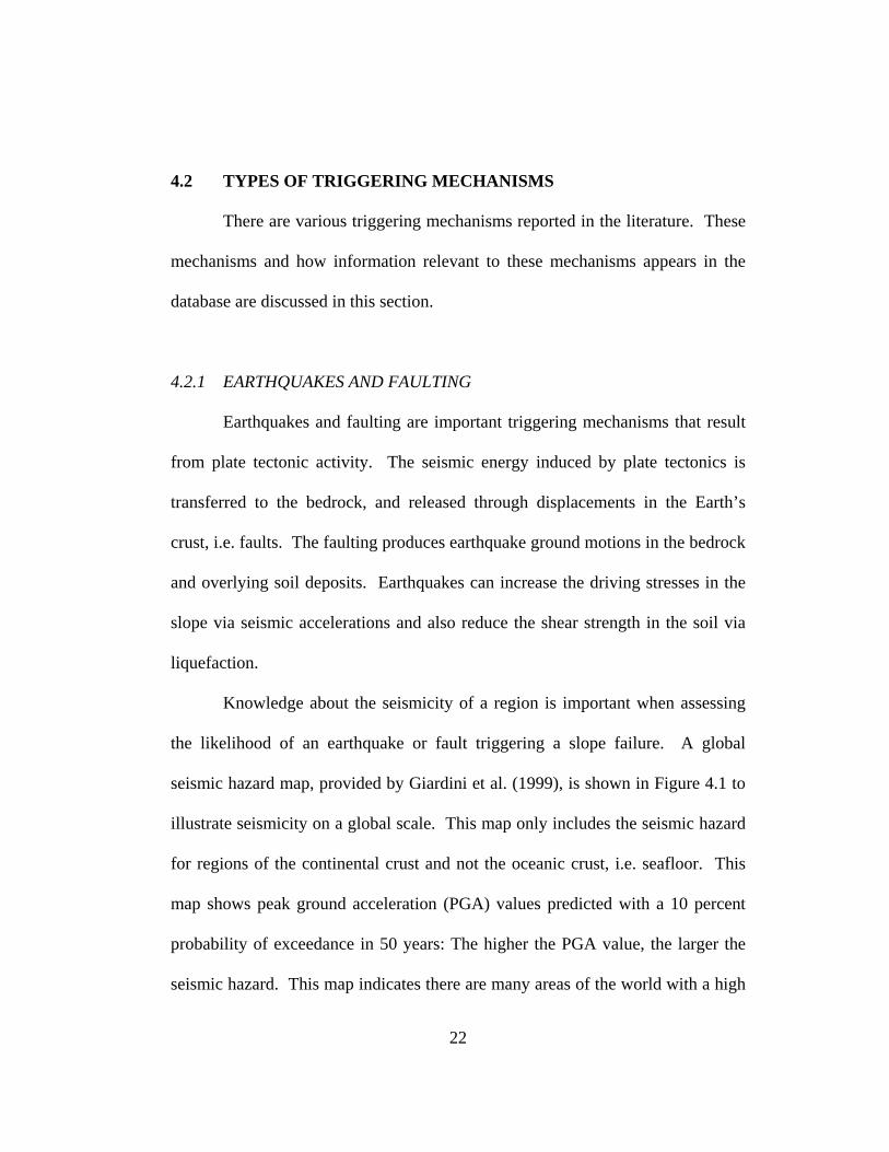
seismic hazard map, provided by Giardini et al. (1999), is shown in Figure 4.1 to
illustrate seismicity on a global scale. This map only includes the seismic hazard
for regions of the continental crust and not the oceanic crust, i.e. seafloor. This
map shows peak ground acceleration (PGA) values predicted with a 10 percent
probability of exceedance in 50 years: The higher the PGA value, the larger the
seismic hazard. This map indicates there are many areas of the world with a high
22
seismic hazard. A field with the geographic coordinates of the slope failures
(Section 3.2.4) was included in the database so that landslides believed to be
triggered by earthquakes and faulting could later be mapped on the global seismic
hazard map to determine any correlations with seismicity. Results of such
correlations are presented in Chapter 5.
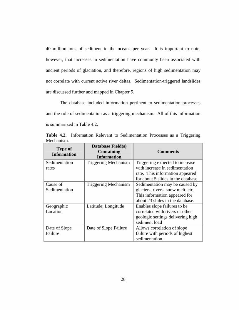
Other information that may be pertinent to earthquakes and faulting was
included in the database, and is summarized in Table 4.1. Table 4.1 also includes
comments regarding the relationship of the information to earthquakes and slope
instability.
Table 4.1. Information Relevant to Earthquakes or Faulting as Triggering Mechanisms.
Type of Information
Database Field(s) Containing Information
Comments
Earthquake Magnitude
Triggering Mechanism
Describes amount of energy that triggered failure. This information appeared for about 22 slides in the database.
Geographic Location of Slope Failure
Latitude; Longitude This information enables mapping of slope failure on global seismic hazard map.
Slope failure location relative to earthquake epicenter location
Slide Description Defines distance between earthquake epicenter and resulting slope failure; This information was available for 6 slides in the database.
Slope location relative to fault location
Triggering Mechanism
Defines distance between fault and resulting slope failure; This information was available for about 50 slides in the database.
23

Table 4.1. Information Relevant to Earthquakes or Faulting as Triggering Mechanisms. (continued)
Type of Information
Database Field(s) Containing Information
Comments
Liquefaction Triggering Mechanism; Slide Description
Liquefaction of soil is typically caused by earthquake shaking and, thus, provides indirect evidence of earthquake-triggered slides; This information was available for about 10 slides in the database.
Geomorphologic Description
Triggering Mechanism; Slide Description
Submarine canyons have been linked to faulting and, thus, provide indirect evidence; This information was rarely provided in the literature.
Type of Slope Failure, e.g. debris flow, slump
Slide Description The type of failure may correlate with the trigger; This information was provided for most earthquake-triggered slides in the database.
Geophysical Description
Triggering Mechanism
Geophysical surveys have revealed the presence of faulting in the subsurface in proximity to slope failure.
Description of seismic activity, e.g. number of earthquakes with magnitude greater than 5 over last 50 years
Triggering Mechanism
Earthquakes and faulting can be inferred as a trigger if the slope is located in a region with sufficient seismic activity. This information was available for about 35 slides in the database.
Date of Slope Failure
Date of Slope Failure
Knowing age can correlate with known earthquakes or periods of seismicity
24

25
Table 4.1. Information Relevant to Earthquakes or Faulting as Triggering Mechanisms. (continued)
Type of Information
Database Field(s) Containing Information
Comments
Number of Past Slope Failures
Triggering Mechanism
Describes quantitatively or qualitatively the history of seismically-induced slope failures; This information was rarely provided in the literature
Type of Fault Triggering Mechanism
Defines the type of fault that induced slope failure, e.g. strike-slip; This information was available for about 5 slides in the database.
4.2.2 SEDIMENTATION PROCESSES
Sedimentation processes can affect slope stability in the offshore
environment and were cited as the cause of failure for many of the case histories
examined. Sedimentation processes are complex because they vary significantly
with respect to time and location. Higher sedimentation rates are commonly
associated with glaciation where water from the oceans is transferred to ice caps,
and the sea level drops. As a result, more continental crust is exposed for erosion
and transport to the oceans. Sedimentation processes are influential in most
marine environments including fjords, river deltas, submarine canyon-fan
systems, open continental slopes and oceanic volcanic islands and ridges. The
processes depend on factors such as water depth, distance to source of sediment
(rivers and river deltas), and, according to Booth et al. (1988), physiographic
setting such as canyon walls, broad open slopes, and ridges.

Figure 4.1: Global Seismic Hazard Map. Orange, red and brown colors indicate high levels of seismic hazard due to large peak ground acceleration (PGA) values predicted with a 10 percent probability of exceedance in 50 years. Green, light green and white colors indicate lower levels of seismic hazard (Giardini et al., 1999).
26

Sedimentation processes can cause slope failure in a variety of direct and
indirect ways. For example, Terzaghi (1956) noted that rapid sediment deposition
can produce an increase in total stresses at a rate faster than the rate of dissipation
of excess pore water pressures. This leads to underconsolidation of soils and
correspondingly low shear strength. Sedimentation can also indirectly trigger
slope failures by creating an environment conducive to other triggering
mechanisms. For example, the accumulation of sediment also contributes to
formation of salt diapirs and steeper slopes (Section 4.2.9). One of the
requirements for the formation of mud volcanoes described in Section 4.2.10 is
rapid sedimentation. If a slope does not fail directly due to sediment loads, the
excess pore water pressures that are created in the soil may leave the slope
marginally stable with factors of safety near unity. If another triggering
mechanism, such as fault rupture, develops, the slope may then fail due in part to
the low shear strength.
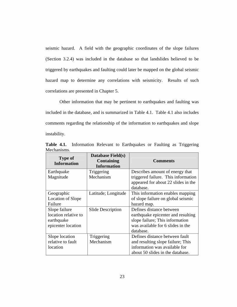
Prior and Coleman (1984) noted that rapid sedimentation is typically
encountered in offshore delta areas and at the base of submarine canyons. Rivers
that deliver the highest sediment load to deltas are shown in Figure 4.2. This
figure includes 22 rivers: Ganges, Yellow (Huangho), Amazon, Yangtze,
Irrawaddy, Magdalena, Mississippi, Orinoco, Red, Mekong, Indus, MacKenzie,
Godavari, La Plata, Purari, Pearl, Copper, Danube, Choshui, Yukon, Niger, Zaire.
According to Milliman and Meade (1983), these rivers each deliver in excess of
27
40 million tons of sediment to the oceans per year. It is important to note,
however, that increases in sedimentation have commonly been associated with
ancient periods of glaciation, and therefore, regions of high sedimentation may
not correlate with current active river deltas. Sedimentation-triggered landslides
are discussed further and mapped in Chapter 5.
The database included information pertinent to sedimentation processes
and the role of sedimentation as a triggering mechanism. All of this information
is summarized in Table 4.2.
Table 4.2. Information Relevant to Sedimentation Processes as a Triggering Mechanism.
Type of Information
Database Field(s) Containing Information
Comments
Sedimentation rates
Triggering Mechanism Triggering expected to increase with increase in sedimentation rate. This information appeared for about 5 slides in the database.
Cause of Sedimentation
Triggering Mechanism Sedimentation may be caused by glaciers, rivers, snow melt, etc. This information appeared for about 23 slides in the database.
Geographic Location
Latitude; Longitude Enables slope failures to be correlated with rivers or other geologic settings delivering high sediment load
Date of Slope Failure
Date of Slope Failure Allows correlation of slope failure with periods of highest sedimentation.
28
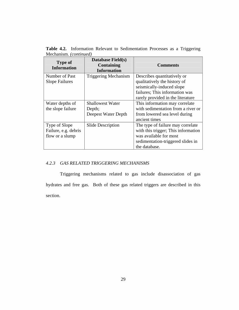
29
Table 4.2. Information Relevant to Sedimentation Processes as a Triggering Mechanism. (continued)
Type of Information
Database Field(s) Containing Information
Comments
Number of Past Slope Failures
Triggering Mechanism Describes quantitatively or qualitatively the history of seismically-induced slope failures; This information was rarely provided in the literature
Water depths of the slope failure
Shallowest Water Depth; Deepest Water Depth
This information may correlate with sedimentation from a river or from lowered sea level during ancient times
Type of Slope Failure, e.g. debris flow or a slump
Slide Description The type of failure may correlate with this trigger; This information was available for most sedimentation-triggered slides in the database.
4.2.3 GAS RELATED TRIGGERING MECHANISMS
Triggering mechanisms related to gas include disassociation of gas
hydrates and free gas. Both of these gas related triggers are described in this
section.

Source: ESRI Data & Maps CDCreated in ArcGIS 8 using ArcMap
Legend
" River Deltas with High Sedimentation
"
"
"
"
""
"
"
"
"
"
"
"
"
"
"
"
"
"
"
Equator
Tropic of Cancer
Tropic of Capricorn
Antarctic Circle
Arctic Circle
Pacific Ocean
Atlantic Ocean
Indian Ocean
Pacific Ocean
-180°
-180°
-160°
-160°
-140°
-140°
-120°
-120°
-100°
-100°
-80°
-80°
-60°
-60°
-40°
-40°
-20°
-20°
0°
0°
20°
20°
40°
40°
60°
60°
80°
80°
100°
100°
120°
120°
140°
140°
160°
160°
180°
180°
0° 0°
-20° -20°
20° 20°
-40° -40°
40° 40°
-60° -60°
60° 60°
-80° -80°
80° 80°
Figure 4.2. Worldwide distribution of river deltas that experience the largest sedimentation rates (sediment discharge data obtained from Milliman and Meade, 1983).
30
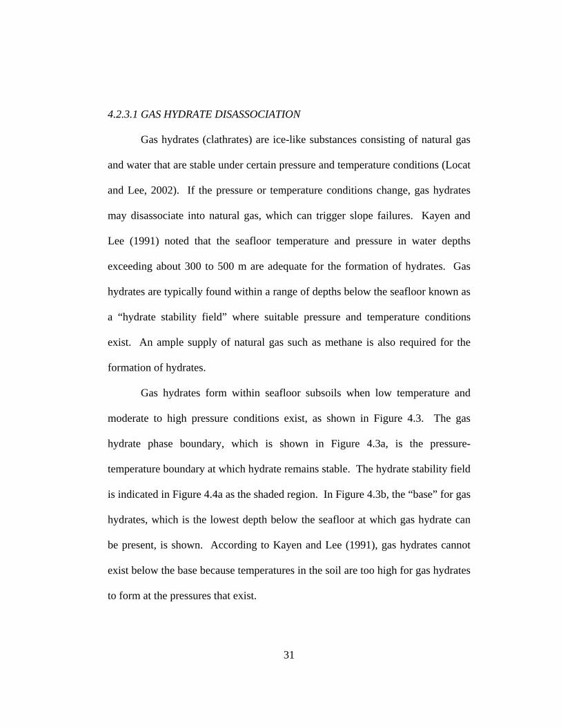
4.2.3.1 GAS HYDRATE DISASSOCIATION
Gas hydrates (clathrates) are ice-like substances consisting of natural gas
and water that are stable under certain pressure and temperature conditions (Locat
and Lee, 2002). If the pressure or temperature conditions change, gas hydrates
may disassociate into natural gas, which can trigger slope failures. Kayen and
Lee (1991) noted that the seafloor temperature and pressure in water depths
exceeding about 300 to 500 m are adequate for the formation of hydrates. Gas
hydrates are typically found within a range of depths below the seafloor known as
a “hydrate stability field” where suitable pressure and temperature conditions
exist. An ample supply of natural gas such as methane is also required for the
formation of hydrates.
Gas hydrates form within seafloor subsoils when low temperature and
moderate to high pressure conditions exist, as shown in Figure 4.3. The gas
hydrate phase boundary, which is shown in Figure 4.3a, is the pressure-
temperature boundary at which hydrate remains stable. The hydrate stability field
is indicated in Figure 4.4a as the shaded region. In Figure 4.3b, the “base” for gas
hydrates, which is the lowest depth below the seafloor at which gas hydrate can
be present, is shown. According to Kayen and Lee (1991), gas hydrates cannot
exist below the base because temperatures in the soil are too high for gas hydrates
to form at the pressures that exist.
31
32
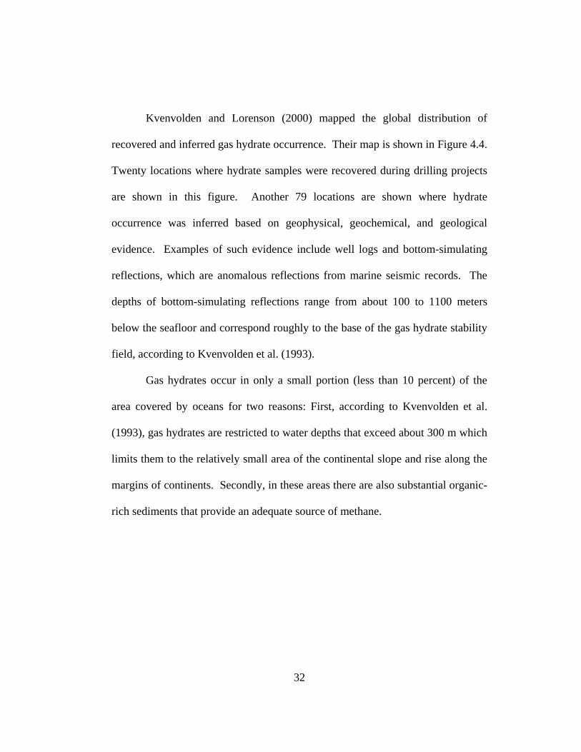
Kvenvolden and Lorenson (2000) mapped the global distribution of
recovered and inferred gas hydrate occurrence. Their map is shown in Figure 4.4.
Twenty locations where hydrate samples were recovered during drilling projects
are shown in this figure. Another 79 locations are shown where hydrate
occurrence was inferred based on geophysical, geochemical, and geological
evidence. Examples of such evidence include well logs and bottom-simulating
reflections, which are anomalous reflections from marine seismic records. The
depths of bottom-simulating reflections range from about 100 to 1100 meters
below the seafloor and correspond roughly to the base of the gas hydrate stability
field, according to Kvenvolden et al. (1993).
Gas hydrates occur in only a small portion (less than 10 percent) of the
area covered by oceans for two reasons: First, according to Kvenvolden et al.
(1993), gas hydrates are restricted to water depths that exceed about 300 m which
limits them to the relatively small area of the continental slope and rise along the
margins of continents. Secondly, in these areas there are also substantial organic-
rich sediments that provide an adequate source of methane.

Gas Hydrate phase boundary
Hydrate Stability Field
(a)
Geothermal Gradient
Base of Gas Hydrate
(b)
Figure 4.3. (a) A pressure-temperature phase diagram for gas hydrate. Shaded region is the hydrate stability field where gas hydrates can exist due to suitable temperature and pressure conditions. (b) A schematic of an offshore slope, indicating the zone in the subsurface where gas hydrate is present. Section A-A′, drawn through the slope, is shown in the phase diagram shown in (a) with the temperature and pressure conditions (modified from Kayen and Lee, 1991).
33

Figure 4.4. Worldwide distribution of gas hydrate occurrence. Black circles indicate inferred gas hydrate occurrence based on bottom-simulating reflections and well logs. White circles indicate recovered gas hydrate samples obtained from drilling projects (Kvenvolden and Lorenson, 2000).
34

Gas hydrates may be the direct trigger of a slope failure, or they may be
associated with other triggering mechanisms. For example, according to Milkov
(2000), gas hydrates typically form around the central part of mud volcanoes,
which are described in Section 4.2.8.
Locat and Lee (2002) noted that a drop in sea level, which reduces the
pressure acting on the seafloor, can cause gas hydrates to disassociate. When gas
hydrates disassociate, the natural gas that is released as bubbles induces total
stresses, σ, and excess pore air pressures, ūa, and excess pore water pressures, ūw,
within the soil deposit, due to the low permeability of most marine soils. Thus,
effective stresses in the sediment, σ΄, are reduced, i.e.
)( wwaa uuuuu +++−=−=′ σσσ . The shear strength is also reduced, and
slope failure occurs. A seafloor slope failure due to gas hydrate disassociation is
shown in Figure 4.5.
Increased temperatures can also cause gas hydrate disassociation. For
example, global warming or warming of the seafloor by changes in current flow
patterns may cause gas hydrates to disassociate. These possibilities may be of
more immediate interest than the next glacial age, which would be expected to be
associated with a drop in sea level as discussed in Section 4.2.14.
35
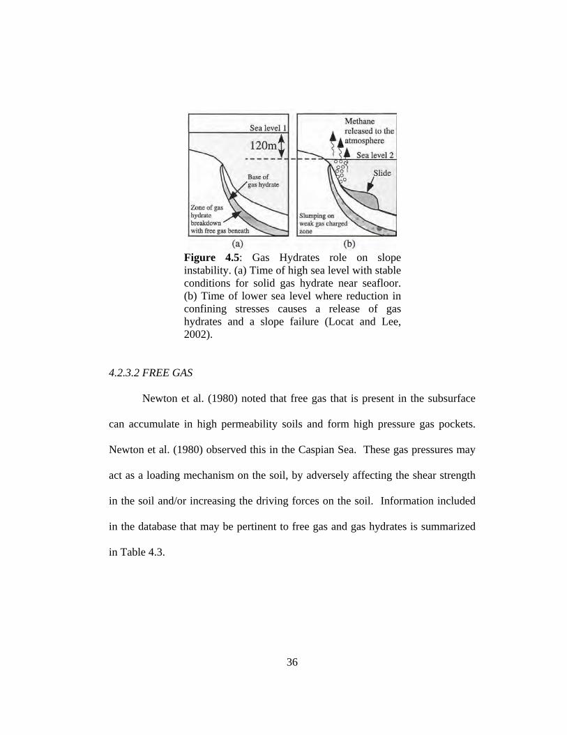
Figure 4.5: Gas Hydrates role on slope instability. (a) Time of high sea level with stable conditions for solid gas hydrate near seafloor. (b) Time of lower sea level where reduction in confining stresses causes a release of gas hydrates and a slope failure (Locat and Lee, 2002).
4.2.3.2 FREE GAS
Newton et al. (1980) noted that free gas that is present in the subsurface
can accumulate in high permeability soils and form high pressure gas pockets.
Newton et al. (1980) observed this in the Caspian Sea. These gas pressures may
act as a loading mechanism on the soil, by adversely affecting the shear strength
in the soil and/or increasing the driving forces on the soil. Information included
in the database that may be pertinent to free gas and gas hydrates is summarized
in Table 4.3.
36
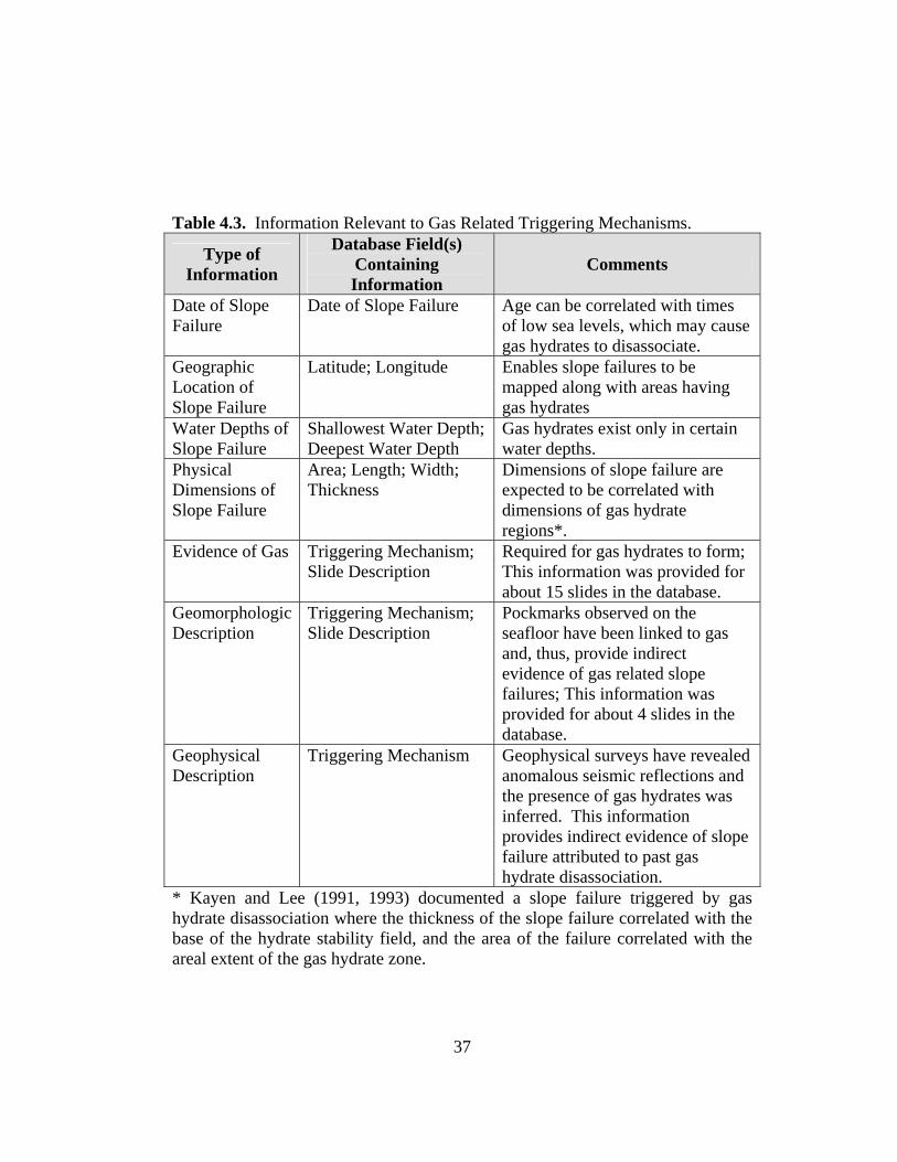
Table 4.3. Information Relevant to Gas Related Triggering Mechanisms.
Type of Information
Database Field(s) Containing Information
Comments
Date of Slope Failure
Date of Slope Failure Age can be correlated with times of low sea levels, which may cause gas hydrates to disassociate.
Geographic Location of Slope Failure
Latitude; Longitude Enables slope failures to be mapped along with areas having gas hydrates
Water Depths of Slope Failure
Shallowest Water Depth; Deepest Water Depth
Gas hydrates exist only in certain water depths.
Physical Dimensions of Slope Failure
Area; Length; Width; Thickness
Dimensions of slope failure are expected to be correlated with dimensions of gas hydrate regions*.
Evidence of Gas Triggering Mechanism; Slide Description
Required for gas hydrates to form; This information was provided for about 15 slides in the database.
Geomorphologic Description
Triggering Mechanism; Slide Description
Pockmarks observed on the seafloor have been linked to gas and, thus, provide indirect evidence of gas related slope failures; This information was provided for about 4 slides in the database.
Geophysical Description
Triggering Mechanism Geophysical surveys have revealed anomalous seismic reflections and the presence of gas hydrates was inferred. This information provides indirect evidence of slope failure attributed to past gas hydrate disassociation.
* Kayen and Lee (1991, 1993) documented a slope failure triggered by gas hydrate disassociation where the thickness of the slope failure correlated with the base of the hydrate stability field, and the area of the failure correlated with the areal extent of the gas hydrate zone.
37
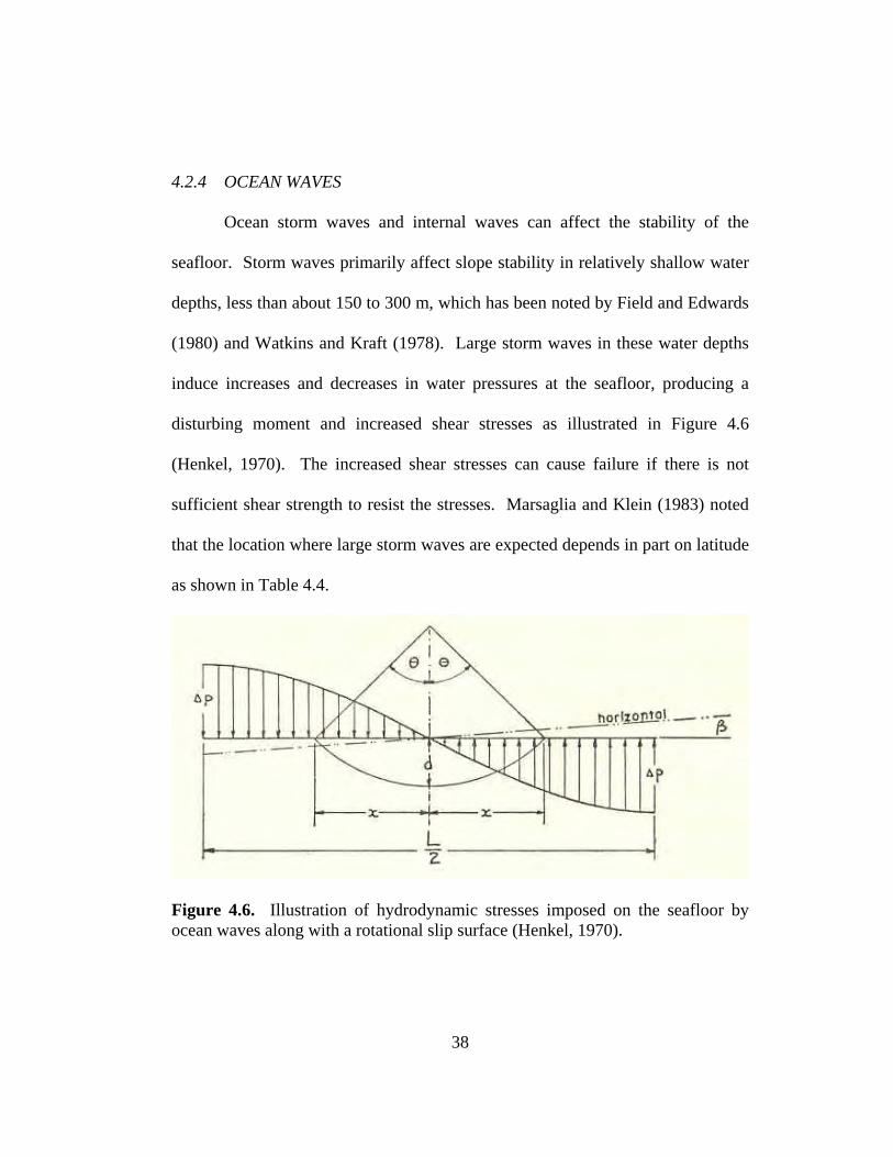
4.2.4 OCEAN WAVES
Ocean storm waves and internal waves can affect the stability of the
seafloor. Storm waves primarily affect slope stability in relatively shallow water
depths, less than about 150 to 300 m, which has been noted by Field and Edwards
(1980) and Watkins and Kraft (1978). Large storm waves in these water depths
induce increases and decreases in water pressures at the seafloor, producing a
disturbing moment and increased shear stresses as illustrated in Figure 4.6
(Henkel, 1970). The increased shear stresses can cause failure if there is not
sufficient shear strength to resist the stresses. Marsaglia and Klein (1983) noted
that the location where large storm waves are expected depends in part on latitude
as shown in Table 4.4.
Figure 4.6. Illustration of hydrodynamic stresses imposed on the seafloor by ocean waves along with a rotational slip surface (Henkel, 1970).
38

Table 4.4. Frequency of storm systems according to latitude (Marsaglia and Klein, 1983).
Latitude Range (degrees) Storm Systems
Above 45 Frequent winter storms, very rare hurricanes
25 – 45 Common winter storms, occasional* hurricanes
5 – 25 Occasional* winter storms, occasional* hurricanes
0 – 5 Very little storm activity of any kind
* “Occasional” denotes probability of occurrence. An occasional winter storms indicates one to two storms per year. An occasional hurricane occurs once in every 3,000 years. However, the Gulf of Mexico is a notable exception where hurricanes are much more frequent.
Another type of wave that can affect the stability of the seafloor is an
internal wave. Internal waves are subsurface current waves. There is evidence of
high velocities associated with internal waves, for example, offshore southern
California as documented by Field and Edwards (1980). In deep water (greater
than a few hundred meters), low-frequency internal waves can transport
sediments along continental slopes and consequently, affect slope stability.
However, according to Field and Edwards (1980), the quantity of sediment
transported by internal waves is not known, and is expected to fluctuate over
time. Information pertinent to ocean waves as a potential triggering mechanism
for seafloor slides that was included in the database is shown in Table 4.5.
39

Table 4.5. Information in the Database Relevant to Ocean Waves as a Potential Triggering Mechanism.
Type of Information
Database Field(s) Containing Information
Comments
Oceanographic Conditions
Triggering Mechanism Description of oceanographic conditions can relate to ocean waves as a trigger. Descriptions include “cyclic loading by storm waves” and “bottom water [soil] movements”; This information was provided for about 5 slides in the database.
Geographic Location of Slope Failure
Latitude; Longitude Storm wave activity is related to latitude.
Water Depths of Slope Failure
Shallowest Water Depth; Deepest Water Depth
Ocean waves primarily affect seafloor stability in water depths less than about 150 to 300 m.
4.2.5 TIDAL EVENTS
Tides are natural, daily events that occur along the coastlines of oceans
and seas. According to Terzaghi (1956), low tide events can trigger slope failure
similar to the way that drawdown effects the upstream slope of an earth dam or
the banks of a river after a flood. Considering undrained conditions, which
typically apply to fine-grained soil deposits, a sudden lowering of water along a
slope at the shoreline removes the resisting forces provided by the external water
along the slope. The factor of safety may be reduced under these conditions by a
factor of up to one half. With regard to coarse-grained soils, seepage forces can
develop when the tide retreats and groundwater flows toward the ocean. Seepage
40
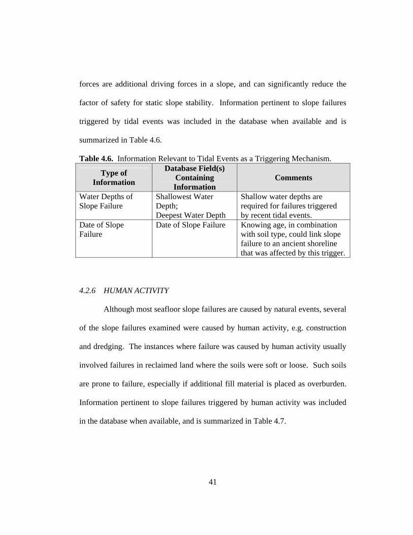
forces are additional driving forces in a slope, and can significantly reduce the
factor of safety for static slope stability. Information pertinent to slope failures
triggered by tidal events was included in the database when available and is
summarized in Table 4.6.
Table 4.6. Information Relevant to Tidal Events as a Triggering Mechanism.
Type of Information
Database Field(s) Containing Information
Comments
Water Depths of Slope Failure
Shallowest Water Depth; Deepest Water Depth
Shallow water depths are required for failures triggered by recent tidal events.
Date of Slope Failure
Date of Slope Failure Knowing age, in combination with soil type, could link slope failure to an ancient shoreline that was affected by this trigger.
4.2.6 HUMAN ACTIVITY
Although most seafloor slope failures are caused by natural events, several
of the slope failures examined were caused by human activity, e.g. construction
and dredging. The instances where failure was caused by human activity usually
involved failures in reclaimed land where the soils were soft or loose. Such soils
are prone to failure, especially if additional fill material is placed as overburden.
Information pertinent to slope failures triggered by human activity was included
in the database when available, and is summarized in Table 4.7.
41

Table 4.7. Information Relevant to Human Activity as a Triggering Mechanism.
Type of Information
Database Field Containing Information
Comments
Date of Slope Failure
Triggering Mechanism Allows correlation of slope failure with times of human activity, e.g. construction.
Type of Damage Slide Description Damage reports from the literature of seafloor slope failures included shoreline facilities and loss of life. These reports are typically linked to slides attributed to human activity.
Type of human activity
Triggering Mechanism Types of human activities included construction, fill placement, and dredging.
4.2.7 EROSION PROCESSES
Erosion occurs in the offshore environment due to water currents that
travel along the seafloor. Erosion combines with sedimentation to change the
seafloor slope by removing sediment from one area and depositing it in another
area. Erosion depends on many of the same factors that affect sedimentation.
Erosion processes can produce slope failure by oversteepening a slope.
Morgenstern (1967) has noted that oversteepening may be local, leading to
progressive slope failure, or global.
Although no slope failures reported in the literature were definitively
attributed to erosion, information pertinent to erosion processes was included in
the database, and is summarized in Table 4.8.
42
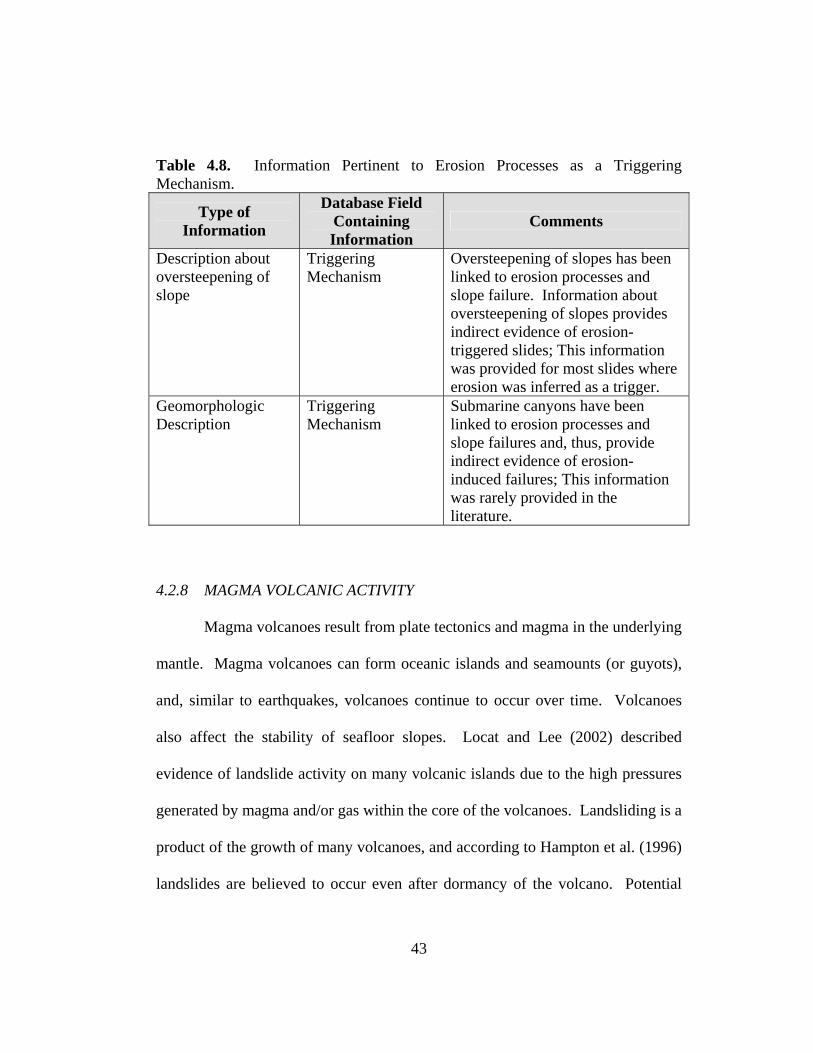
Table 4.8. Information Pertinent to Erosion Processes as a Triggering Mechanism.
Type of Information
Database Field Containing Information
Comments
Description about oversteepening of slope
Triggering Mechanism
Oversteepening of slopes has been linked to erosion processes and slope failure. Information about oversteepening of slopes provides indirect evidence of erosion-triggered slides; This information was provided for most slides where erosion was inferred as a trigger.
Geomorphologic Description
Triggering Mechanism
Submarine canyons have been linked to erosion processes and slope failures and, thus, provide indirect evidence of erosion-induced failures; This information was rarely provided in the literature.
4.2.8 MAGMA VOLCANIC ACTIVITY
Magma volcanoes result from plate tectonics and magma in the underlying
mantle. Magma volcanoes can form oceanic islands and seamounts (or guyots),
and, similar to earthquakes, volcanoes continue to occur over time. Volcanoes
also affect the stability of seafloor slopes. Locat and Lee (2002) described
evidence of landslide activity on many volcanic islands due to the high pressures
generated by magma and/or gas within the core of the volcanoes. Landsliding is a
product of the growth of many volcanoes, and according to Hampton et al. (1996)
landslides are believed to occur even after dormancy of the volcano. Potential
43
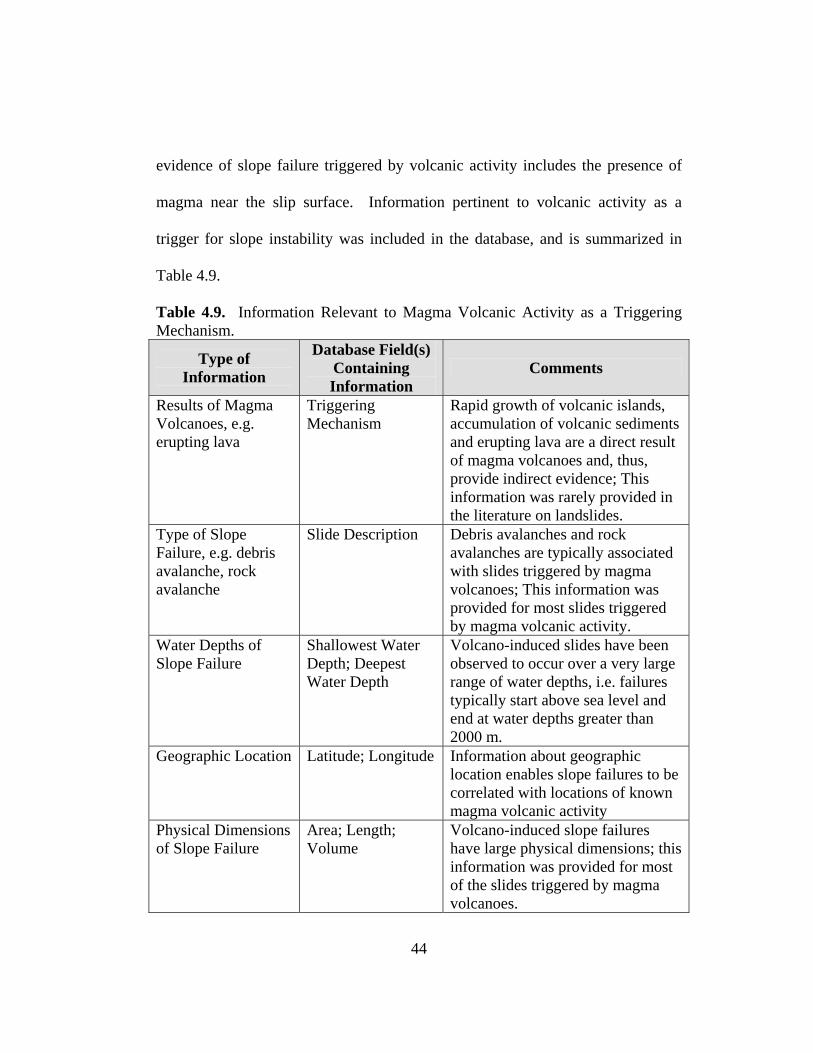
evidence of slope failure triggered by volcanic activity includes the presence of
magma near the slip surface. Information pertinent to volcanic activity as a
trigger for slope instability was included in the database, and is summarized in
Table 4.9.
Table 4.9. Information Relevant to Magma Volcanic Activity as a Triggering Mechanism.
Type of Information
Database Field(s) Containing Information
Comments
Results of Magma Volcanoes, e.g. erupting lava
Triggering Mechanism
Rapid growth of volcanic islands, accumulation of volcanic sediments and erupting lava are a direct result of magma volcanoes and, thus, provide indirect evidence; This information was rarely provided in the literature on landslides.
Type of Slope Failure, e.g. debris avalanche, rock avalanche
Slide Description Debris avalanches and rock avalanches are typically associated with slides triggered by magma volcanoes; This information was provided for most slides triggered by magma volcanic activity.
Water Depths of Slope Failure
Shallowest Water Depth; Deepest Water Depth
Volcano-induced slides have been observed to occur over a very large range of water depths, i.e. failures typically start above sea level and end at water depths greater than 2000 m.
Geographic Location Latitude; Longitude Information about geographic location enables slope failures to be correlated with locations of known magma volcanic activity
Physical Dimensions of Slope Failure
Area; Length; Volume
Volcano-induced slope failures have large physical dimensions; this information was provided for most of the slides triggered by magma volcanoes.
44
4.2.9 SALT DIAPIRISM
Salt diapirs can form in the subsurface of the seafloor due to cycles of
flooding and evaporation over geologic time. The geologic history of the Gulf of
Mexico provides a good illustration of the formation processes associated with
salt diapirs. During the Jurassic period (about 213 to 144 million years ago), the
Gulf of Mexico became isolated from the oceans, and a thick sequence of salt
(Louann Salt) accumulated as water evaporated from the Gulf. During the
Jurassic period, the Gulf was a smaller basin than today with a more restricted
opening for water to enter. The Gulf would periodically flood, and then become
completely dry, forming a salt plain. As sediments were later deposited in the
basin by flood waters, the weight of the sediments caused the underlying salt to
deform plastically. McGregor et al. (1993) noted that after the salt plains formed
an enormous amount of sediment was deposited. In response to the weight of the
overlying sediment, salt tended to rise to the surface, deforming plastically in the
process. As this occurred, numerous fingers of salt, also known as diapirs, moved
upward through the sediment. The term diapir is from the Greek word
“diapeirein” which means “to pierce” according to O’Brien (1968).
Diapiric activity causes the seafloor to deform plastically over time. The
growth of diapirs is proportional to the thickness of salt available for movement
and the amount of overburden stresses. Overburden stresses depend on the
density of the sediment and the rates of sediment accumulation and erosion. In
45
46
areas of diapiric activity, the slope of the seafloor is a result of a complex
relationship between overburden sediment loading (sediment accumulation) and
diapiric growth. Diapirs can create a bathymetric low by increasing slope angles,
which can result in an intraslope basin. An example of such a basin created from
adjacent diapiric uplifting is shown in Figure 4.7. Intraslope basins become
locations where sediment can accumulate at higher rates than along higher angle,
adjacent slopes. As a result, additional diapirs can then later form within this
basin. Seafloor slope angles evolve over time, and the corresponding bathymetry
becomes more complex. The complex bathymetry mapped along the Texas-
Louisiana slope is shown in Figure 4.8, and the corresponding masses of salt and
shale along the Texas-Louisiana slope are shown in Figure 4.9. Evidence of the
effects of diapiric activity is shown in Figures 4.8 and 4.9.
Slope failure occurs due to diapiric activity. Soil slopes continue to fail by
slumping due to the increasing slope angles in areas of diapiric activity. A slump
that was mapped in a region of diapiric uplift is shown in Figure 4.7. The
pressures induced by the underlying mobile salt may act as a loading mechanism
on the overlying soil slope. If the soil is fine-grained and has a low permeability,
excess pore water pressures would be generated. Thus, the shear strength and
factor of safety for slope stability would be reduced.

Figure 4.7: Seismic reflection profile across diapiric uplift in upper continental slope off Western Louisiana showing slumping (Martin and Bouma, 1982).
47
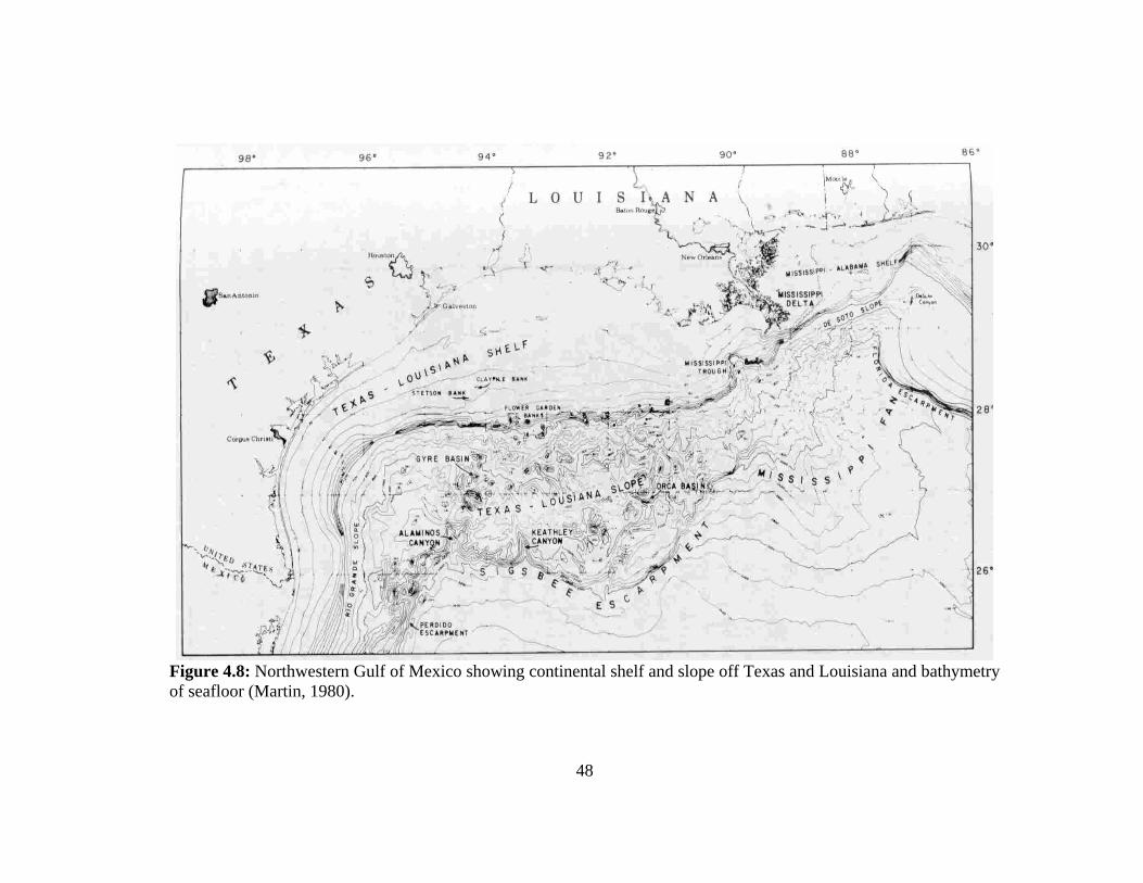
Figure 4.8: Northwestern Gulf of Mexico showing continental shelf and slope off Texas and Louisiana and bathymetry of seafloor (Martin, 1980).
48

Figure 4.9: Location of structurally active thick masses of Jurassic salt and Tertiary shale (Martin and Bouma, 1982).
There are also areas other than the Gulf of Mexico where diapiric activity
is evident. Diapiric activity has been reported along the South and mid-Atlantic
U.S. continental slope, Norwegian-Greenland Sea, Beringian margin (Alaska),
Gulf of Guinea (West Africa), northern Sinai-southern Israel continental slope,
and the Sao Paulo Embayment (Brazil-Uruguay continental margin). Information
pertinent to salt diapirism that was included in the database is summarized in
Table 4.10.
49
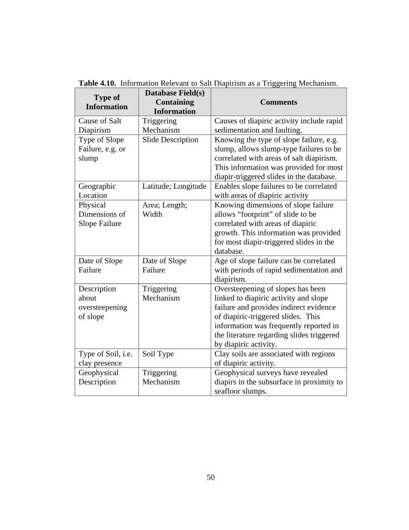
Table 4.10. Information Relevant to Salt Diapirism as a Triggering Mechanism.
Type of Information
Database Field(s) Containing Information
Comments
Cause of Salt Diapirism
Triggering Mechanism
Causes of diapiric activity include rapid sedimentation and faulting.
Type of Slope Failure, e.g. or slump
Slide Description Knowing the type of slope failure, e.g. slump, allows slump-type failures to be correlated with areas of salt diapirism. This information was provided for most diapir-triggered slides in the database.
Geographic Location
Latitude; Longitude Enables slope failures to be correlated with areas of diapiric activity
Physical Dimensions of Slope Failure
Area; Length; Width
Knowing dimensions of slope failure allows “footprint” of slide to be correlated with areas of diapiric growth. This information was provided for most diapir-triggered slides in the database.
Date of Slope Failure
Date of Slope Failure
Age of slope failure can be correlated with periods of rapid sedimentation and diapirism.
Description about oversteepening of slope
Triggering Mechanism
Oversteepening of slopes has been linked to diapiric activity and slope failure and provides indirect evidence of diapiric-triggered slides. This information was frequently reported in the literature regarding slides triggered by diapiric activity.
Type of Soil, i.e. clay presence
Soil Type Clay soils are associated with regions of diapiric activity.
Geophysical Description
Triggering Mechanism
Geophysical surveys have revealed diapirs in the subsurface in proximity to seafloor slumps.
50

4.2.10 MUD VOLCANIC ACTIVITY
Submarine mud volcanoes are raised features on the seafloor that erupt
mud, gas and fluids such as water and oil. The possible ways mud volcanoes
form are illustrated in Figure 4.10. The formation of mud volcanoes requires high
gas or fluid pressures within the subsurface and fluid migration either along a
compression fault (Figure 4.10c, d, e) or via a diapir that pierces the seafloor
(Figure 4.10b). In addition to high pressures and fluid migration, high
sedimentation rates (Section 4.2.2) are often required to promote diapiric growth
so that mud volcanoes can occur. According to Newton et al. (1980), mud
volcanoes can also be reactivated periodically due to gas pressures, faulting,
diapirism, and sedimentation, which are all recurring triggering mechanisms.
d e b ca
Figurwithoseaflofault; the sefluid
e 4.10. Possible ways mut a mud volcano; (b)or-piercing diapir; (c) (d, e) Mud volcanoes foafloor along compressi
travel (Milkov, 2000).
ud volcanoes Mud volcano Fluid forming armed due to flu
on faults. Arro
51
can form. (a) Diapir formed on top of a long a compression id transported up to ws indicate path of
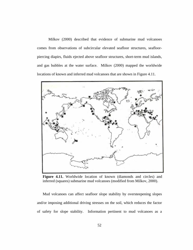
Milkov (2000) described that evidence of submarine mud volcanoes
comes from observations of subcircular elevated seafloor structures, seafloor-
piercing diapirs, fluids ejected above seafloor structures, short-term mud islands,
and gas bubbles at the water surface. Milkov (2000) mapped the worldwide
locations of known and inferred mud volcanoes that are shown in Figure 4.11.
Figure 4.11. Worldwide location of known (diamonds and circles) and inferred (squares) submarine mud volcanoes (modified from Milkov, 2000).
Mud volcanoes can affect seafloor slope stability by oversteepening slopes
and/or imposing additional driving stresses on the soil, which reduces the factor
of safety for slope stability. Information pertinent to mud volcanoes as a
52

triggering mechanism that was included in the database is summarized in Table
4.11.
Table 4.11. Information Relevant to Mud Volcanoes as a Triggering Mechanism.
Type of Information
Database Field(s) Containing Information
Comments
Evidence of other triggering mechanisms
Triggering Mechanism
Rapid sedimentation, compression faulting, diapirs and high gas pressures have been linked to mud volcanoes and, thus, provide indirect evidence of mud volcanoes as a triggering mechanism.
Geographic Location
Latitude; Longitude Geographic location of major mud volcanic activity is known, and by knowing the location of slope failures, correlations between slope failure and mud volcanic activity should be possible.
4.2.11 FLOOD EVENTS
Flood events often produce rapid sedimentation in coastal regions and
river deltas (Section 4.2.2). High sedimentation rates caused by flooding may
increase driving stresses on the seafloor sediments, leading to failure. Flood
events may also erode river deltas, leading to turbidity currents, or low density
landslides.
Only two landslides in the database were actually attributed to flood
events. Information that may be relevant to flood events and was included in the
database is summarized in Table 4.12.
53
Table 4.12. Information Pertinent to Flood Events as a Triggering Mechanism. Type of
Information Database Field
Containing Information Comments
Cause of Flood Event
Slide Description Snowmelt and glacier melt have been linked to flooding and, thus, may provide indirect evidence of slides triggered by flood events.
Erosion of river deltas
Triggering Mechanism Erosion of river deltas (sand bars) has been linked to flooding and slope failure, i.e. turbidity current formation, and provides indirect evidence of seafloor slides attributed to flooding.
4.2.12 CREEP
Creep is generally defined as strain that develops under constant load.
Creep is a time-dependent, slow process and can involve large masses of soil.
Creep can occur under either drained or undrained loading conditions.
Although creep is poorly understood as a mechanism for seafloor slope
movement, creep has been attributed to mass movement processes in the
literature. For example, Field and Edwards (1980) mention sediment creep as a
slope movement process offshore southern California. Information pertinent to
creep that was included in the database is summarized in Table 4.13.
54
Table 4.13. Information Relevant to Creep as a Triggering Mechanism.
Type of Information
Database Field(s) Containing Information
Comments
Geomorphologic Description
Slide Description; Triggering Mechanism
Lack of a distinct failure scar has been linked to creep-induced sliding.
Geophysical Description
Triggering Mechanism
Geophysical surveys have revealed internal deformation within seafloor subsoils, which have been linked to creep.
4.2.13 TSUNAMIS
Tsunamis are large ocean waves triggered by seismic events or submarine
landslides, rather than by ocean storm events. Tsunamis can affect slope stability
in two ways: First, tsunamis can induce large hydrodynamic stresses on the
seafloor. Secondly, tsunamis can also lower water levels as they approach
shorelines, causing rapid drawdown (Wright and Rathje, in press). The rapid
lowering of the water level without time for drainage of the soil reduces the
resisting force of the body of water with no change in soil shear strength, thus
reducing the factor of safety. There were no slope failures in the database directly
caused by tsunamis. However, information relevant to tsunamis that was
included in the database is summarized in Table 4.14.
55
Table 4.14. Information Pertinent to Tsunamis as a Triggering Mechanism. Type of
Information Database Field(s)
Containing Information Comments
Linking tsunami and slope failures
Slide Description Soils deposited by tsunamis have been linked to slope failures and, thus, provide indirect evidence of slope failures attributed to tsunamis.
Date of slope failure
Triggering Mechanism; Date of Slope Failure
Allows correlation of slope failure with periods of seismic activity, which often triggers the tsunami.
4.2.14 SEA-LEVEL FLUCTUATIONS
Sea level fluctuations are primarily caused by changes in global climate.
Sea level fluctuations can cause slope failures in several ways. A fall in sea level
reduces the overall pressure applied on the sea floor, which can result in
disassociation of gas hydrates (Section 4.2.3) which can trigger slope failure. A
fall in sea level can also promote an increase in sedimentation (Section 4.2.2),
which can trigger landslides. McGuire (1992) noted that a rise in sea level can
lead to erosion of the flanks of volcanic islands, which results in steepening of the
slope and eventual slope failure. Sea level changes also affect the pressures
acting on magma volcanoes, and McGuire (1992) noted that large changes in
water pressure on the seafloor may increase magmatic activity and cause
formation of volcanic islands (Section 4.2.8) and eventual landsliding.
56
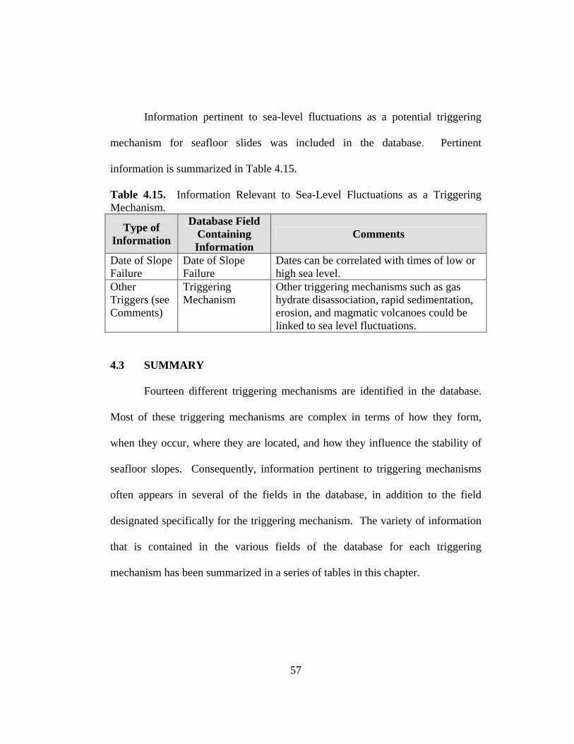
Information pertinent to sea-level fluctuations as a potential triggering
mechanism for seafloor slides was included in the database. Pertinent
information is summarized in Table 4.15.
Table 4.15. Information Relevant to Sea-Level Fluctuations as a Triggering Mechanism.
Type of Information
Database Field Containing Information
Comments
Date of Slope Failure
Date of Slope Failure
Dates can be correlated with times of low or high sea level.
Other Triggers (see Comments)
Triggering Mechanism
Other triggering mechanisms such as gas hydrate disassociation, rapid sedimentation, erosion, and magmatic volcanoes could be linked to sea level fluctuations.
4.3 SUMMARY
Fourteen different triggering mechanisms are identified in the database.
Most of these triggering mechanisms are complex in terms of how they form,
when they occur, where they are located, and how they influence the stability of
seafloor slopes. Consequently, information pertinent to triggering mechanisms
often appears in several of the fields in the database, in addition to the field
designated specifically for the triggering mechanism. The variety of information
that is contained in the various fields of the database for each triggering
mechanism has been summarized in a series of tables in this chapter.
57
CHAPTER 5
EVALUATION OF CHARACTERISTICS OF SLOPE FAILURES
IN THE DATABASE
5.1 INTRODUCTION
Once the database was created, the data were examined to determine
important characteristics of the failures and trends in the data. The following
characteristics of the slopes failures were examined:
• geographic location
• date of the failure
• soil type
• triggering mechanism(s)
• distance of slide runout
• slide thickness
• slide area
• slide volume
• slope angle
• shallowest and deepest water depths for the slide mass
The database contained fields for each of these characteristics. Queries were then
written to extract information from these fields. Information from the queries was
then exported to Microsoft Excel® where plots of the information were made. In
58
addition, world maps were created showing the location of slope failures for
selected triggering mechanisms. The maps were created using the geographic
coordinate data in the database and the ArcGIS® software. The results of this
effort are presented in this chapter.
5.2 CHARACTERISTICS OF THE DATA
A summary of the numbers of slope failures for which data were available
for each particular field in the database is presented in Table 5.1. The percentage
of the total number of events that contains each type of data is shown in the last
column of this table.
59
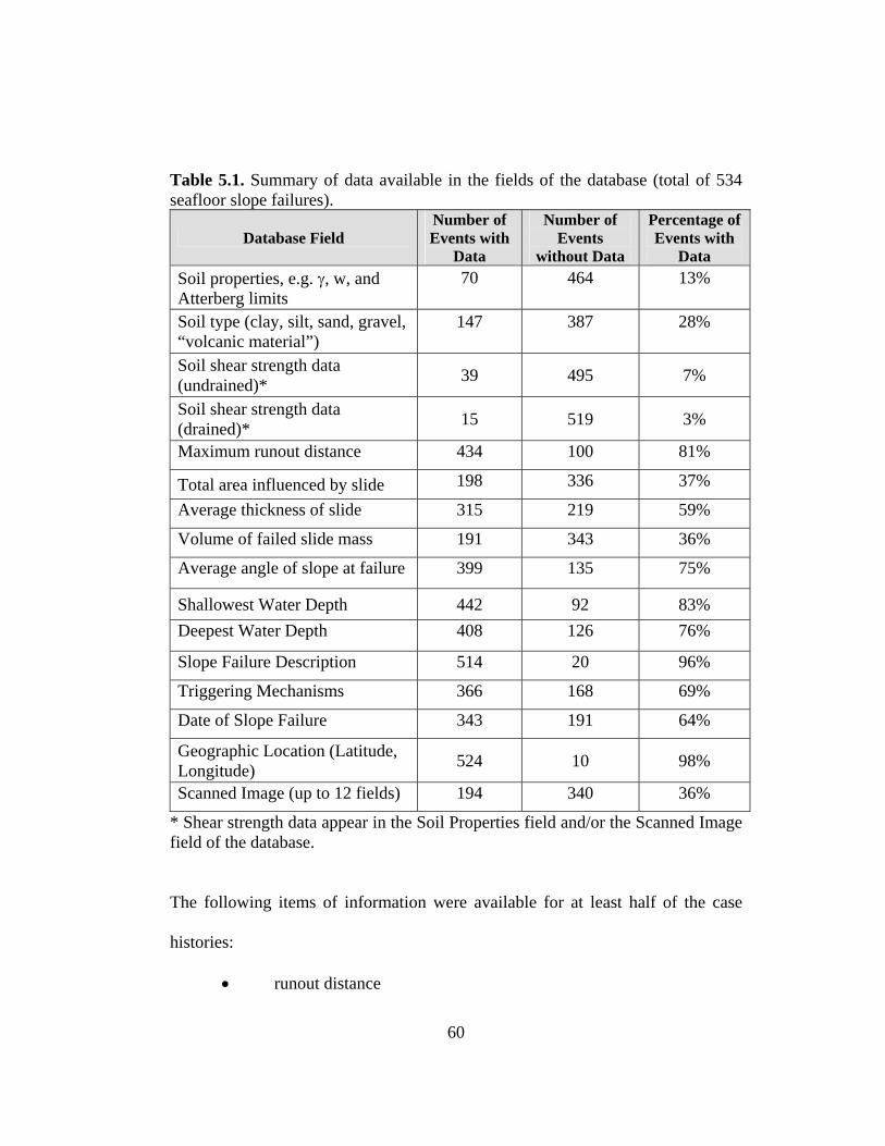
Table 5.1. Summary of data available in the fields of the database (total of 534 seafloor slope failures).
Database Field Number of Events with
Data
Number of Events
without Data
Percentage of Events with
Data Soil properties, e.g. γ, w, and Atterberg limits
70 464 13%
Soil type (clay, silt, sand, gravel, “volcanic material”)
147 387 28%
Soil shear strength data (undrained)* 39 495 7%
Soil shear strength data (drained)* 15 519 3%
Maximum runout distance 434 100 81%
Total area influenced by slide 198 336 37%
Average thickness of slide 315 219 59%
Volume of failed slide mass 191 343 36%
Average angle of slope at failure 399 135 75%
Shallowest Water Depth 442 92 83% Deepest Water Depth 408 126 76%
Slope Failure Description 514 20 96%
Triggering Mechanisms 366 168 69%
Date of Slope Failure 343 191 64%
Geographic Location (Latitude, Longitude) 524 10 98%
Scanned Image (up to 12 fields) 194 340 36%
* Shear strength data appear in the Soil Properties field and/or the Scanned Image field of the database.
The following items of information were available for at least half of the case
histories:
• runout distance
60
• slide thickness
• average angle of slope at failure
• water depths of the failure
• slide description
• triggering mechanisms
• date of the slope failure
• geographic location
Some visual description of the slope failure was available for 194 of the slides.
The visual description was captured in the Scanned Image field of the database.
More than one scanned image was available for the majority of the 194 slides.
The database contains over 520 images.
Although there is substantial information in the database, most slope
failures lacked significant geotechnical information. Only about 10 percent of the
case histories have information about the shear strength of the soil. Less than
one-third of the slides have a description of the type of soil, and only about one-
eighth of the slides have a description of the properties of the soil. The lack of
geotechnical information can probably be attributed to the inherent cost and
difficulties in obtaining this information. Site specific soil information is
typically acquired and owned by oil companies, and is not published.
61
5.3 DATE OF SLOPE FAILURES
Information was available on the date of the slope failure for 343 of the
534 slide events in the database. The literature used to extract this information
contained the date of failure in two forms. In 299 of the 343 cases, the date was
reported in terms of a geologic epoch. In the remaining 44 cases, the date was
reported as a specific date, and the failures generally occurred within the last few
hundred years. Many of these latter 44 failures involve known earthquake events
where the investigators report that the earthquake event was a possible trigger for
the slope failure, i.e. the date of the slope failure was assumed to be the same as
the date of the earthquake.
A plot of the frequency distribution of slope failures according to geologic
epoch is shown in Figure 5.1. Figure 5.1 and the frequency distributions in the
following sections of this chapter are plotted as bar charts where the slides in each
interval represent a percentage of the total number of slides for which the
appropriate data were available. The 44 failures that occurred (or were inferred to
occur) within the last few hundred years were included in Figure 5.1 under the
column for Holocene Epoch, i.e. within the last 10,000 years (10 ka). The
Pleistocene Epoch is prior to the Holocene, and is between approximately 1.6
million years (1.6 Ma) and 10 ka before present. The Pliocene Epoch is before
the Pleistocene, and is between approximately 5.3 Ma and 1.6 Ma before present.
The case histories for which data are available are divided approximately equally
62

between the Holocene and Pleistocene Epochs. Only about 5 percent of the slope
failures where date of failure data were available occurred in the Pliocene Epoch.
Several of the triggering mechanisms such as rapid sedimentation, gas hydrate
disassociation, and salt diapirism have been linked with times of low sea level
which occurred during Holocene and late Pleistocene Epochs, and this may
account for why most of the slope failures occurred during these epochs. Also,
slides that occurred during these epochs are the most recent, so they are easier to
detect than older slides.
0
10
20
30
40
50
60
Holocene Pleistocene Pliocene
time (Geologic Epoch)
Freq
uenc
y (%
)
343 events
Figure 5.1. Frequency distribution of approximate date of slope failures.
63
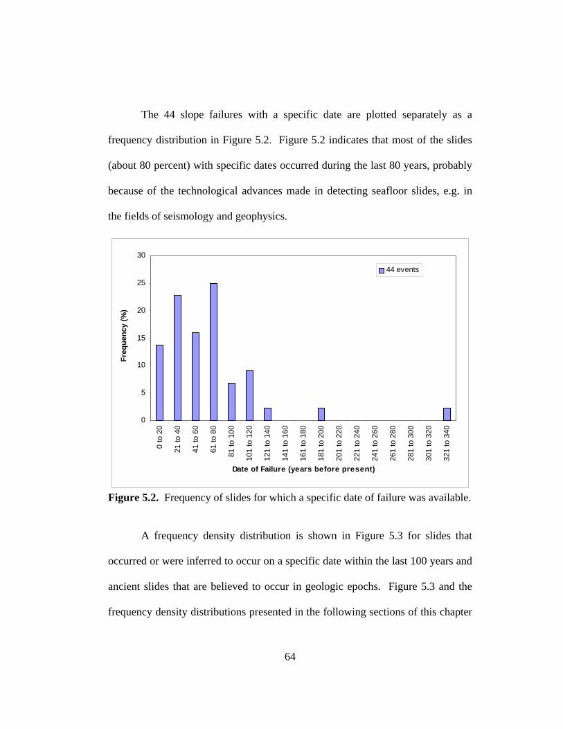
The 44 slope failures with a specific date are plotted separately as a
frequency distribution in Figure 5.2. Figure 5.2 indicates that most of the slides
(about 80 percent) with specific dates occurred during the last 80 years, probably
because of the technological advances made in detecting seafloor slides, e.g. in
the fields of seismology and geophysics.
0
5
10
15
20
25
30
0 to
20
21 to
40
41 to
60
61 to
80
81 to
100
101
to 1
20
121
to 1
40
141
to 1
60
161
to 1
80
181
to 2
00
201
to 2
20
221
to 2
40
241
to 2
60
261
to 2
80
281
to 3
00
301
to 3
20
321
to 3
40
Date of Failure (years before present)
Freq
uenc
y (%
)
44 events
Figure 5.2. Frequency of slides for which a specific date of failure was available.
A frequency density distribution is shown in Figure 5.3 for slides that
occurred or were inferred to occur on a specific date within the last 100 years and
ancient slides that are believed to occur in geologic epochs. Figure 5.3 and the
frequency density distributions presented in the following sections of this chapter
64
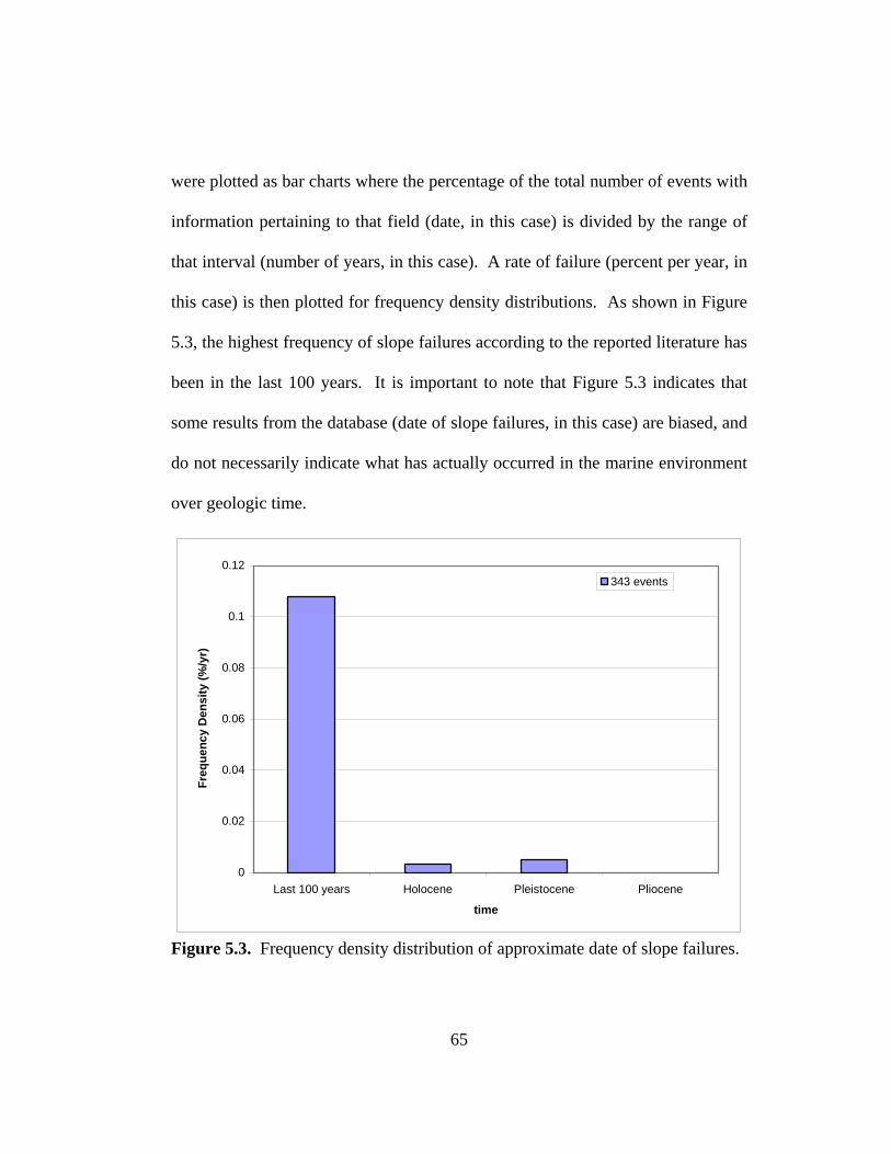
were plotted as bar charts where the percentage of the total number of events with
information pertaining to that field (date, in this case) is divided by the range of
that interval (number of years, in this case). A rate of failure (percent per year, in
this case) is then plotted for frequency density distributions. As shown in Figure
5.3, the highest frequency of slope failures according to the reported literature has
been in the last 100 years. It is important to note that Figure 5.3 indicates that
some results from the database (date of slope failures, in this case) are biased, and
do not necessarily indicate what has actually occurred in the marine environment
over geologic time.
0
0.02
0.04
0.06
0.08
0.1
0.12
Last 100 years Holocene Pleistocene Pliocene
time
Freq
uenc
y D
ensi
ty (%
/yr)
343 events
Figure 5.3. Frequency density distribution of approximate date of slope failures.
65
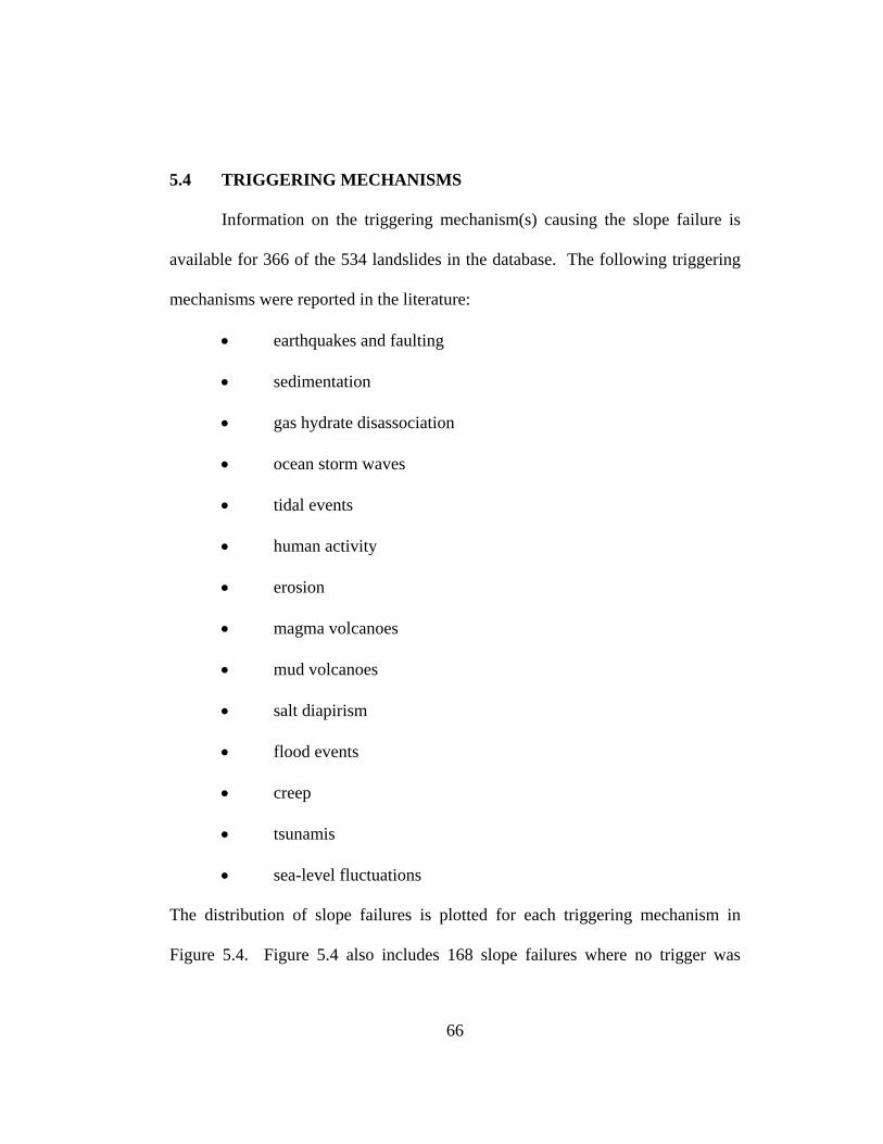
5.4 TRIGGERING MECHANISMS
Information on the triggering mechanism(s) causing the slope failure is
available for 366 of the 534 landslides in the database. The following triggering
mechanisms were reported in the literature:
• earthquakes and faulting
• sedimentation
• gas hydrate disassociation
• ocean storm waves
• tidal events
• human activity
• erosion
• magma volcanoes
• mud volcanoes
• salt diapirism
• flood events
• creep
• tsunamis
• sea-level fluctuations
The distribution of slope failures is plotted for each triggering mechanism in
Figure 5.4. Figure 5.4 also includes 168 slope failures where no trigger was
66
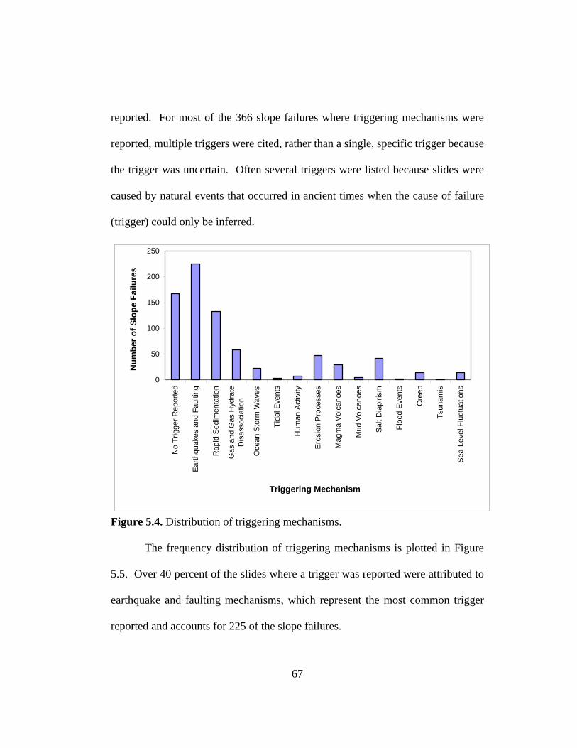
reported. For most of the 366 slope failures where triggering mechanisms were
reported, multiple triggers were cited, rather than a single, specific trigger because
the trigger was uncertain. Often several triggers were listed because slides were
caused by natural events that occurred in ancient times when the cause of failure
(trigger) could only be inferred.
0
50
100
150
200
250
No
Trig
ger R
epor
ted
Earth
quak
es a
nd F
aulti
ng
Rap
id S
edim
enta
tion
Gas
and
Gas
Hyd
rate
Dis
asso
ciat
ion
Oce
an S
torm
Wav
es
Tida
l Eve
nts
Hum
an A
ctiv
ity
Eros
ion
Proc
esse
s
Mag
ma
Volc
anoe
s
Mud
Vol
cano
es
Salt
Dia
piris
m
Floo
d Ev
ents
Cre
ep
Tsun
amis
Sea-
Leve
l Flu
ctua
tions
Triggering Mechanism
Num
ber o
f Slo
pe F
ailu
res
Figure 5.4. Distribution of triggering mechanisms.
The frequency distribution of triggering mechanisms is plotted in Figure
5.5. Over 40 percent of the slides where a trigger was reported were attributed to
earthquake and faulting mechanisms, which represent the most common trigger
reported and accounts for 225 of the slope failures.
67
The frequencies of slides that were inferred and were known to be
triggered by earthquakes are summarized in Table 5.2. Earthquakes were inferred
to be the trigger for 86 percent of the slides, but earthquakes were only known to
be the trigger for 14 percent of the slides.
Table 5.2. Qualification of data regarding the 225 earthquake-triggered seafloor slope failures captured in the database.
Type of Information Number of Events Fraction of Total (%)
Inferred 193 86 Known 32 14
Geologic processes of sedimentation and erosion account for about 25 and
9 percent, respectively, of the potential triggers for slope failure (Figure 5.5).
Ocean storm waves, tidal events, flood events and human activity were cited in
less than 5 percent of the landslide events. Ocean storm waves, tidal events, flood
events and human activity tend to influence slopes in water shallower than a few
hundred meters. On a global scale, most ocean water is deeper than a few
hundred meters, where ocean storm waves, tidal events, flood events and human
activity (construction along shorelines) are not possible triggers.
Gas hydrate disassociation is cited as a possible trigger for about 11
percent of the landslides. This percentage may reflect the fact that gas hydrates
are present in about 10 percent of the seafloor area covered by oceans (Chapter
4). Volcanic and diapiric activity are described as triggers in less than 10 percent
68
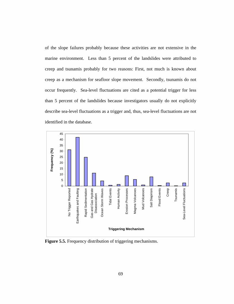
of the slope failures probably because these activities are not extensive in the
marine environment. Less than 5 percent of the landslides were attributed to
creep and tsunamis probably for two reasons: First, not much is known about
creep as a mechanism for seafloor slope movement. Secondly, tsunamis do not
occur frequently. Sea-level fluctuations are cited as a potential trigger for less
than 5 percent of the landslides because investigators usually do not explicitly
describe sea-level fluctuations as a trigger and, thus, sea-level fluctuations are not
identified in the database.
0
5
10
15
20
25
30
35
40
45
No
Trig
ger R
epor
ted
Ear
thqu
akes
and
Fau
lting
Rap
id S
edim
enta
tion
Gas
and
Gas
Hyd
rate
Dis
asso
ciat
ion
Oce
an S
torm
Wav
es
Tida
l Eve
nts
Hum
an A
ctiv
ity
Ero
sion
Pro
cess
es
Mag
ma
Vol
cano
es
Mud
Vol
cano
es
Sal
t Dia
piris
m
Floo
d E
vent
s
Cre
ep
Tsun
amis
Sea
-Lev
el F
luct
uatio
ns
Triggering Mechanism
Freq
uenc
y (%
)
Figure 5.5. Frequency distribution of triggering mechanisms.
69
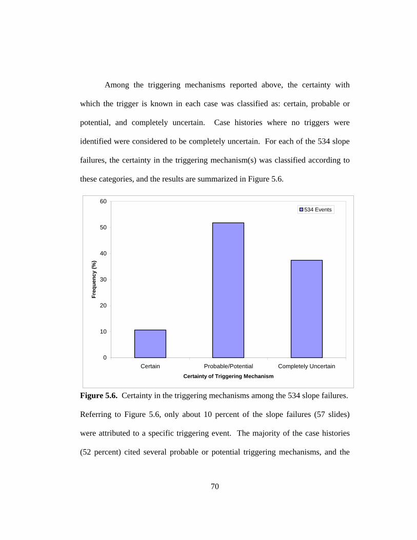
Among the triggering mechanisms reported above, the certainty with
which the trigger is known in each case was classified as: certain, probable or
potential, and completely uncertain. Case histories where no triggers were
identified were considered to be completely uncertain. For each of the 534 slope
failures, the certainty in the triggering mechanism(s) was classified according to
these categories, and the results are summarized in Figure 5.6.
0
10
20
30
40
50
60
Certain Probable/Potential Completely UncertainCertainty of Triggering Mechanism
Freq
uenc
y (%
)
534 Events
Figure 5.6. Certainty in the triggering mechanisms among the 534 slope failures.
Referring to Figure 5.6, only about 10 percent of the slope failures (57 slides)
were attributed to a specific triggering event. The majority of the case histories
(52 percent) cited several probable or potential triggering mechanisms, and the
70
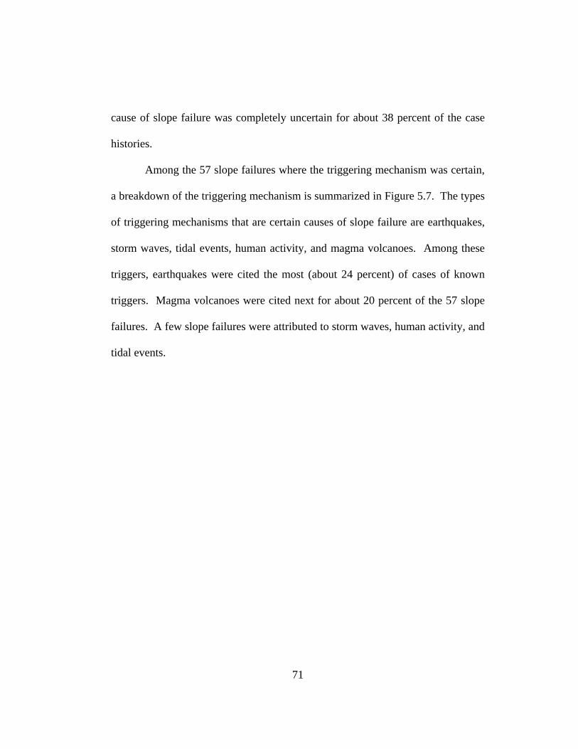
cause of slope failure was completely uncertain for about 38 percent of the case
histories.
Among the 57 slope failures where the triggering mechanism was certain,
a breakdown of the triggering mechanism is summarized in Figure 5.7. The types
of triggering mechanisms that are certain causes of slope failure are earthquakes,
storm waves, tidal events, human activity, and magma volcanoes. Among these
triggers, earthquakes were cited the most (about 24 percent) of cases of known
triggers. Magma volcanoes were cited next for about 20 percent of the 57 slope
failures. A few slope failures were attributed to storm waves, human activity, and
tidal events.
71

0
5
10
15
20
25
Earthquakes Storm Waves Tidal Events Human Activity Magma VolcanicActivity
Known Triggering Mechanism
Num
ber o
f Slo
pe F
ailu
res
57 Events
Figure 5.7. Types of triggering mechanisms among the 57 slides with known triggers.
For about 15 of the 57 slides where the trigger was certain, conclusive
evidence was provided by an “eyewitness” account. Eyewitness accounts include
observing damage to an offshore structure, a shoreline structure or
communication cables buried in the seafloor. Linking the trigger such as a
hurricane or an earthquake, with the slide that caused the damage is possible due
to such eyewitness accounts.
72
5.5 GEOGRAPHIC LOCATION OF SLOPE FAILURES
The geographic location was reported for almost all of the seafloor slides
(524 out of 534) in the database. Latitude and longitude were extracted from the
literature and recorded in the database for each slope failure. The geographic
coordinates were then exported from the database to Excel® to generate figures
summarizing the results. The distributions of slope failures by latitude and by
longitude are summarized in Figures 5.8 and 5.9, respectively.
The majority of the slope failures are located in the northern and western
hemispheres of the world as shown in Figures 5.8 and 5.9, respectively. These
locations are probably indicative of where offshore exploration has occurred and
data have been published. Consequently, these locations are probably not
indicative of the frequency of landslides worldwide.
73

0
50
100
150
200
250
300
80 to 61S
60 to 41S
40 to 21S
20 to 0 S 0 to 20 N 21 to 40N
41 to 60N
61 to 80N
80 to 90N
Latitude (degrees)
Num
ber o
f Slo
pe F
ailu
res
524 Events
Figure 5.8. Distribution of submarine landslides by latitude.
74
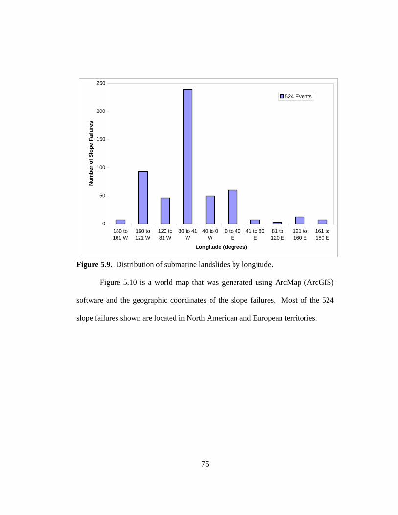
75
0
50
180 to161 W
160 to121 W
120 to81 W
80 to 41W
40 to 0W
0 to 40E
41 to 80E
Longitude (degrees)
Num
ber o
f Slo
pe F
ailu
res
100
150
200
250
81 to120 E
121 to160 E
161 to180 E
524 Events
Figure 5.9. Distribution of submarine landslides by longitude.
Figure 5.10 is a world map that was generated using ArcMap (ArcGIS)
software and the geographic coordinates of the slope failures. Most of the 524
slope failures shown are located in North American and European territories.
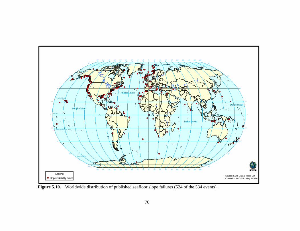
Equator
Tro pic of Can cer
Trop ic o f Capricorn
Antarctic Circle
Arctic Circle
Pacific Ocean
Atlantic Ocean
Indian Ocean
Pacific Ocean
-180°
-180°
-160°
-160°
-140°
-140°
-120°
-120°
-100°
-100°
-80°
-80°
-60°
-60°
-40°
-40°
-20°
-20°
0°
0°
20°
20°
40°
40°
60°
60°
80°
80°
100°
100°
120°
120°
140°
140°
160°
160°
180°
180°
0° 0°
-20° -20°
20° 20°
-40° -40°
40° 40°
-60° -60°
60° 60°
-80° -80°
80° 80°
Source: ESRI Data & Maps CDCreated in ArcGIS 8 using ArcMap
Legendslope instability event
Figure 5.10. Worldwide distribution of published seafloor slope failures (524 of the 534 events).
76

5.6 GEOGRAPHIC DISTRIBUTION OF SLOPE FAILURES FOR VARIOUS TRIGGERING MECHANISMS
The geographic distribution of slope failures was evaluated for six
triggering mechanisms: earthquakes and faulting, rapid sedimentation, gas
hydrate disassociation, ocean storm waves, magma volcanoes, and mud
volcanoes. World maps were created displaying the locations where triggering
events are most likely and the locations of slope failures attributed to the triggers.
5.6.1 EARTHQUAKES AND FAULTING
A global seismic hazard map showing the locations of seafloor slides
thought to be triggered by earthquakes and faulting is shown in Figure 5.11.
Many areas of the world represent a high seismic hazard, and there is a good
correlation between the seismic hazard and slides attributed to seismicity. Most
of the slides shown on the map are in regions that have a moderate to high seismic
hazard. For example, numerous slides believed to be triggered by earthquakes
have occurred near the Pacific coast of the United States, the Gulf of Alaska, and
the region of the Aleutian Islands. These areas all have moderate to high
seismicity.
77

Figure 5.11. Global seismic hazard map (Giardini et al., 1999) with the worldwide distribution of published seafloor
slope failures attributed to seismic loading (seafloor slides noted by black circles).
78
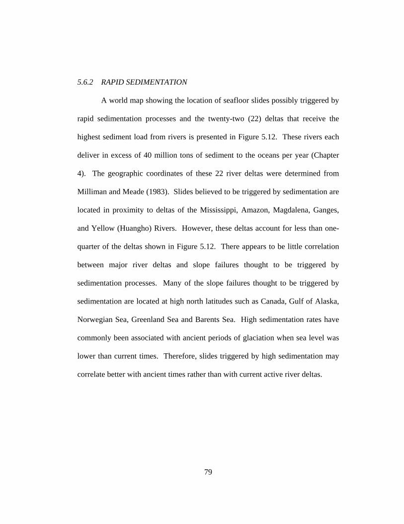
5.6.2 RAPID SEDIMENTATION
A world map showing the location of seafloor slides possibly triggered by
rapid sedimentation processes and the twenty-two (22) deltas that receive the
highest sediment load from rivers is presented in Figure 5.12. These rivers each
deliver in excess of 40 million tons of sediment to the oceans per year (Chapter
4). The geographic coordinates of these 22 river deltas were determined from
Milliman and Meade (1983). Slides believed to be triggered by sedimentation are
located in proximity to deltas of the Mississippi, Amazon, Magdalena, Ganges,
and Yellow (Huangho) Rivers. However, these deltas account for less than one-
quarter of the deltas shown in Figure 5.12. There appears to be little correlation
between major river deltas and slope failures thought to be triggered by
sedimentation processes. Many of the slope failures thought to be triggered by
sedimentation are located at high north latitudes such as Canada, Gulf of Alaska,
Norwegian Sea, Greenland Sea and Barents Sea. High sedimentation rates have
commonly been associated with ancient periods of glaciation when sea level was
lower than current times. Therefore, slides triggered by high sedimentation may
correlate better with ancient times rather than with current active river deltas.
79
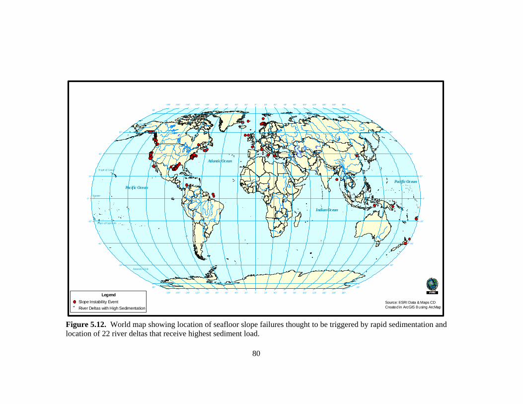
Source: ESRI Data & Maps CDCreated in ArcGIS 8 using ArcMap
LegendSlope Instability Event
" River Deltas with High Sedimentation
"
"
"
"
""
"
"
"
"
"
"
"
"
"
"
"
"
"
"
Equator
Tropic of Cancer
Tropic of Capricorn
Antarctic Circle
Arctic Circle
Pacific Ocean
Atlantic Ocean
Indian Ocean
Pacific Ocean
-180°
-180°
-160°
-160°
-140°
-140°
-120°
-120°
-100°
-100°
-80°
-80°
-60°
-60°
-40°
-40°
-20°
-20°
0°
0°
20°
20°
40°
40°
60°
60°
80°
80°
100°
100°
120°
120°
140°
140°
160°
160°
180°
180°
0° 0°
-20° -20°
20° 20°
-40° -40°
40° 40°
-60° -60°
60° 60°
-80° -80°
80° 80°
Figure 5.12. World map showing location of seafloor slope failures thought to be triggered by rapid sedimentation and location of 22 river deltas that receive highest sediment load.
80

5.6.3 DISASSOCIATION OF GAS HYDRATES
The areas where gas hydrates have been detected and where slope failures
attributed to gas hydrate disassociation have occurred are presented in Figure
5.13. The geographic coordinates of areas where gas hydrates have been detected
were determined from Kvenvolden and Lorenson (2000). In the northern
latitudes, there is fairly good correlation shown in Figure 5.13 between areas
where gas hydrates have been detected and slope failures attributed to gas hydrate
disassociation. Areas where correlation exists include the Gulf of Mexico,
offshore the southeast coast of the United States, offshore Oregon, the Beaufort
Sea, the Norwegian/Barents Sea, the Caspian Sea, and the Black Sea.
81

Source: ESRI Data & Maps CDCreated in ArcGIS 8 using ArcMap
LegendSeafloor slope failures possibly triggered by gas hydrate disassociation
" Areas of Detected Gas Hydrate
""
"
"""""
"
"
"
""""""
"""
"""
""
"
"
""
"
"
"
"
Equator
Tropic of Cancer
Tropic of Capricorn
An tarctic C ircle
Arctic Circle
Pacific Ocean
Atlantic Ocean
Indian Ocean
Pacific Ocean
-180°
-180°
-160°
-160°
-140°
-140°
-120°
-120°
-100°
-100°
-80°
-80°
-60°
-60°
-40°
-40°
-20°
-20°
0°
0°
20°
20°
40°
40°
60°
60°
80°
80°
100°
100°
120°
120°
140°
140°
160°
160°
180°
180°
0° 0°
-20° -20°
20° 20°
-40° -40°
40° 40°
-60° -60°
60° 60°
-80° -80°
80° 80°
Figure 5.13. World map showing location of seafloor slope failures thought to be triggered by gas hydrate disassociation and location of detected gas hydrates.
82

5.6.4 OCEAN STORM WAVES
The distribution of seafloor slides associated with ocean wave loading is
shown in Figure 5.14. About half of the slides shown are located above 40
degrees north latitude where winter storms are common, occurring multiple times
per year. Also, three slides triggered by ocean storm waves are located in the
Gulf of Mexico and along the Atlantic coast of North America where hurricane
systems often travel (Marsaglia and Klein, 1983). Finally, there are several slides
triggered by ocean waves in the Hawaiian Islands, where large waves occur due
to tropical storms (Hayes, 1967). Overall, there is good correlation between
regions of large ocean storm waves and slides attributed to storm waves.
83
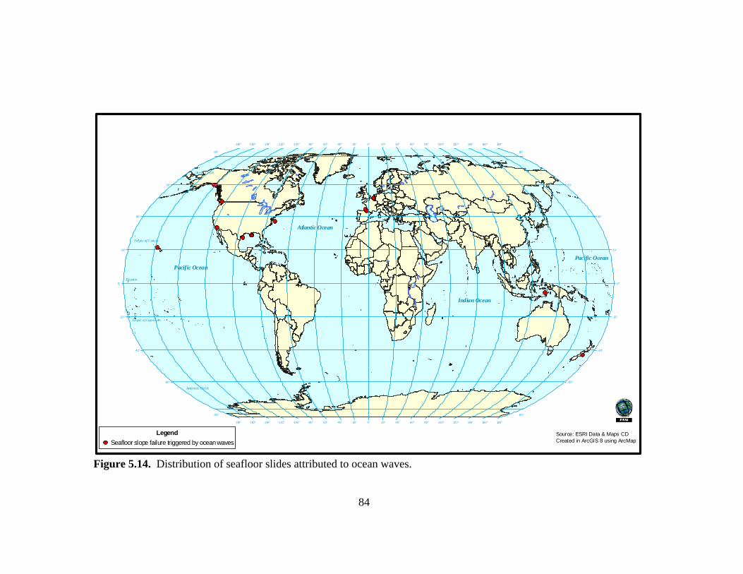
Source: ESRI Data & Maps CDCreated in ArcGIS 8 using ArcMap
LegendSeafloor slope failure triggered by ocean waves
Equator
Tro pic of Cancer
Tropic o f Capricorn
Antarctic Circle
Arctic Circle
Pacific Ocean
Atlantic Ocean
Indian Ocean
Pacific Ocean
-180°
-180°
-160°
-160°
-140°
-140°
-120°
-120°
-100°
-100°
-80°
-80°
-60°
-60°
-40°
-40°
-20°
-20°
0°
0°
20°
20°
40°
40°
60°
60°
80°
80°
100°
100°
120°
120°
140°
140°
160°
160°
180°
180°
0° 0°
-20° -20°
20° 20°
-40° -40°
40° 40°
-60° -60°
60° 60°
-80° -80°
80° 80°
Figure 5.14. Distribution of seafloor slides attributed to ocean waves.
84
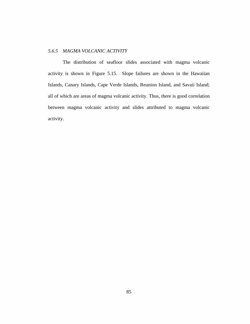
5.6.5 MAGMA VOLCANIC ACTIVITY
The distribution of seafloor slides associated with magma volcanic
activity is shown in Figure 5.15. Slope failures are shown in the Hawaiian
Islands, Canary Islands, Cape Verde Islands, Reunion Island, and Savaii Island;
all of which are areas of magma volcanic activity. Thus, there is good correlation
between magma volcanic activity and slides attributed to magma volcanic
activity.
85

Source: ESRI Data & Maps CDCreated in ArcGIS 8 using ArcMap
Legend
Seafloor slope failure triggered by magma volcanic activity
Equator
Tropic of Cancer
Tropic of Capricorn
Antarctic Circle
Arctic Circle
Pacific Ocean
Atlantic Ocean
Indian Ocean
Pacific Ocean
-180°
-180°
-160°
-160°
-140°
-140°
-120°
-120°
-100°
-100°
-80°
-80°
-60°
-60°
-40°
-40°
-20°
-20°
0°
0°
20°
20°
40°
40°
60°
60°
80°
80°
100°
100°
120°
120°
140°
140°
160°
160°
180°
180°
0° 0°
-20° -20°
20° 20°
-40° -40°
40° 40°
-60° -60°
60° 60°
-80° -80°
80° 80°
Figure 5.15. Distribution of published seafloor slope failures triggered by magma volcanic activity.
86
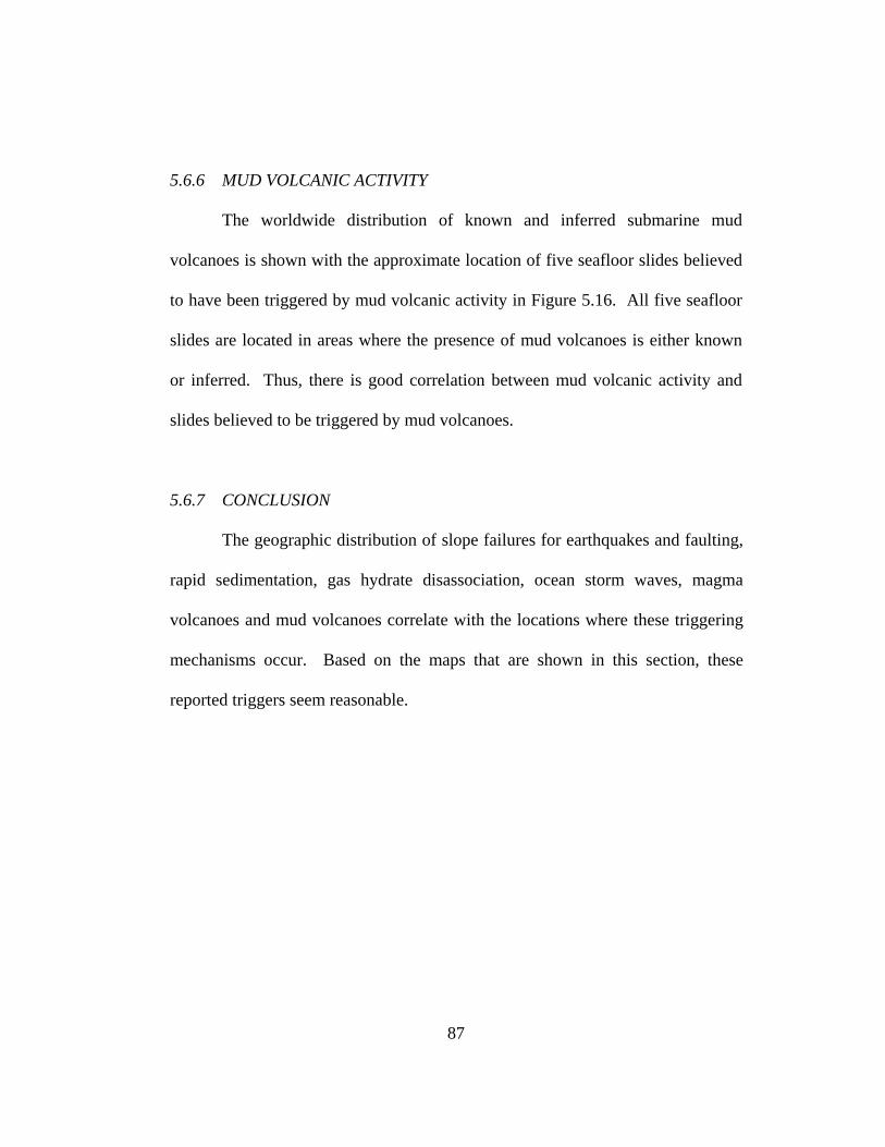
5.6.6 MUD VOLCANIC ACTIVITY
The worldwide distribution of known and inferred submarine mud
volcanoes is shown with the approximate location of five seafloor slides believed
to have been triggered by mud volcanic activity in Figure 5.16. All five seafloor
slides are located in areas where the presence of mud volcanoes is either known
or inferred. Thus, there is good correlation between mud volcanic activity and
slides believed to be triggered by mud volcanoes.
5.6.7 CONCLUSION
The geographic distribution of slope failures for earthquakes and faulting,
rapid sedimentation, gas hydrate disassociation, ocean storm waves, magma
volcanoes and mud volcanoes correlate with the locations where these triggering
mechanisms occur. Based on the maps that are shown in this section, these
reported triggers seem reasonable.
87
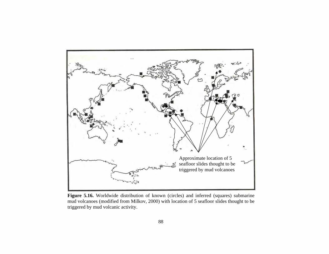
Approximate location of 5 seafloor slides thought to be triggered by mud volcanoes
Figure 5.16. Worldwide distribution of known (circles) and inferred (squares) submarine mud volcanoes (modified from Milkov, 2000) with location of 5 seafloor slides thought to be triggered by mud volcanic activity.
88
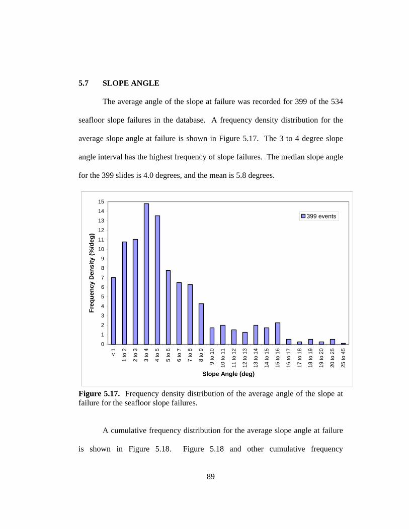
5.7 SLOPE ANGLE
The average angle of the slope at failure was recorded for 399 of the 534
seafloor slope failures in the database. A frequency density distribution for the
average slope angle at failure is shown in Figure 5.17. The 3 to 4 degree slope
angle interval has the highest frequency of slope failures. The median slope angle
for the 399 slides is 4.0 degrees, and the mean is 5.8 degrees.
0
1
2
3
4
5
6
7
8
9
10
11
12
13
14
15
< 1
1 to
2
2 to
3
3 to
4
4 to
5
5 to
6
6 to
7
7 to
8
8 to
9
9 to
10
10 to
11
11 to
12
12 to
13
13 to
14
14 to
15
15 to
16
16 to
17
17 to
18
18 to
19
19 to
20
20 to
25
25 to
45
Slope Angle (deg)
Freq
uenc
y D
ensi
ty (%
/deg
)
399 events
Figure 5.17. Frequency density distribution of the average angle of the slope at failure for the seafloor slope failures.
A cumulative frequency distribution for the average slope angle at failure
is shown in Figure 5.18. Figure 5.18 and other cumulative frequency
89
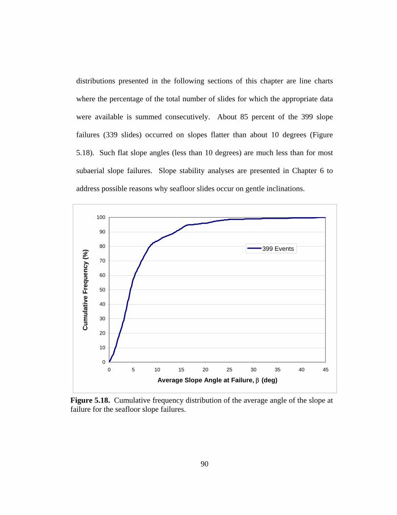
distributions presented in the following sections of this chapter are line charts
where the percentage of the total number of slides for which the appropriate data
were available is summed consecutively. About 85 percent of the 399 slope
failures (339 slides) occurred on slopes flatter than about 10 degrees (Figure
5.18). Such flat slope angles (less than 10 degrees) are much less than for most
subaerial slope failures. Slope stability analyses are presented in Chapter 6 to
address possible reasons why seafloor slides occur on gentle inclinations.
0
10
20
30
40
50
60
70
80
90
100
0 5 10 15 20 25 30 35 40 45
Average Slope Angle at Failure, β (deg)
Cum
ulat
ive
Freq
uenc
y (%
) 399 Events
Figure 5.18. Cumulative frequency distribution of the average angle of the slope at failure for the seafloor slope failures.
90

5.8 DIMENSIONS OF SLOPE FAILURES
The dimensions of the slope failures were characterized by information in
five fields in the database: area, length, width, thickness, and volume. This
information is examined further in this section.
5.8.1 Total Area Influenced by Slope Failure
Information was available on the total area influenced by the slope failure
for 198 of the 534 seafloor slides in the database. A cumulative frequency
distribution of the area of the slope failures is presented in Figure 5.19. Because
of the large range in area (over five orders of magnitude), a logarithmic scale is
used to plot the area. The median area (50th percentile) for the 198 events is
approximately 200 km2, and the mean area is approximately 3,600 km2. The data
shown in Figure 5.19 show that the area of seafloor slides can be very large, on
the order of hundreds to thousands of square kilometers.
91

0
10
20
30
40
50
60
70
80
90
100
1 10 100 1000 10000 100000
Area (km2)
Cum
ulat
ive
Freq
uenc
y (%
)198 Events
Figure 5.19. Cumulative frequency distribution of area influenced by slides.
A frequency density distribution for the total area influenced by the
seafloor slides is plotted in Figure 5.20. The highest frequency of slides involve
areas between about 5 and 10 km2. The second most frequent range in areas is
less than 5 km2. The median area (200 km2) is much smaller than the mean area
(3,600 km2) because slides of smaller areas have a much higher frequency of
occurrence.
Even with the best technology, seafloor slope failures smaller than about
one square kilometer are probably not detected (McAdoo et al., 2000) and, thus,
are inherently excluded from the database. Furthermore, if very small slides were
92
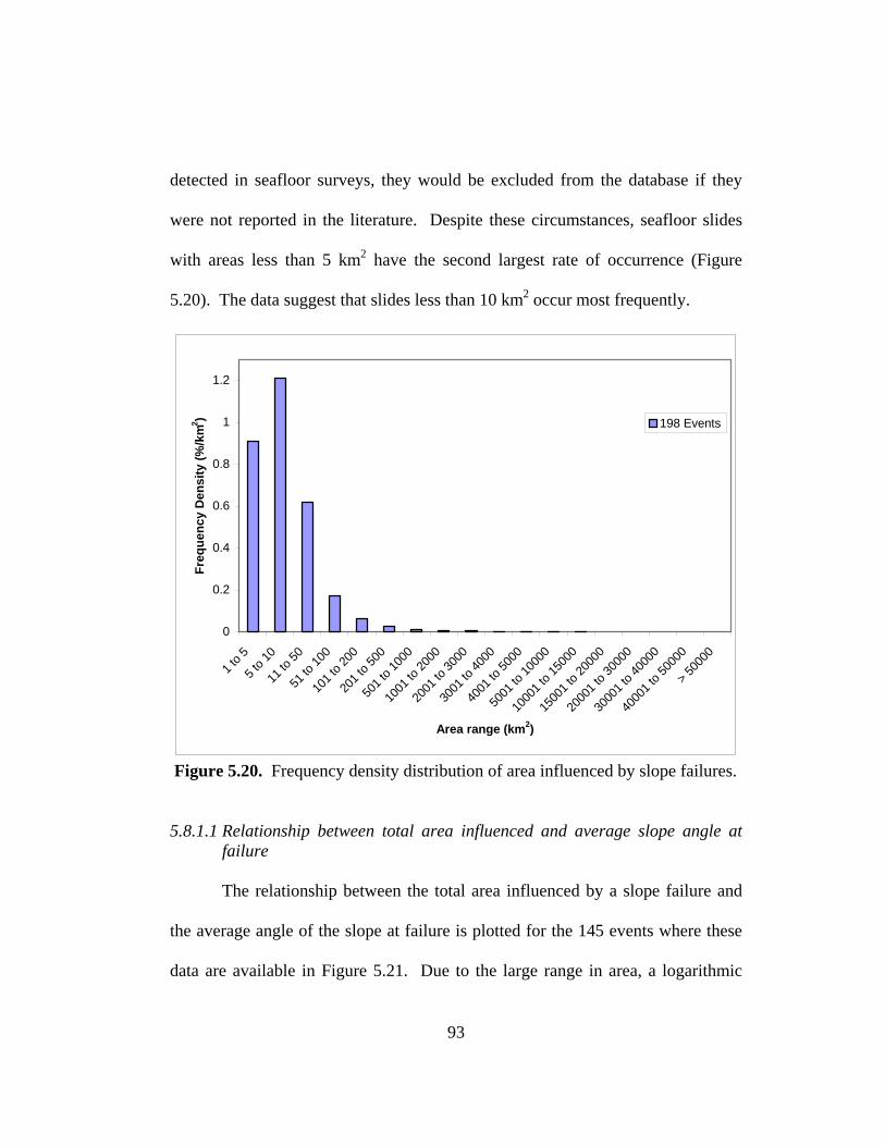
detected in seafloor surveys, they would be excluded from the database if they
were not reported in the literature. Despite these circumstances, seafloor slides
with areas less than 5 km2 have the second largest rate of occurrence (Figure
5.20). The data suggest that slides less than 10 km2 occur most frequently.
0
0.2
0.4
0.6
0.8
1
1.2
1 to 5
5 to 1
0
11 to
50
51 to
100
101 t
o 200
201 t
o 500
501 t
o 100
0
1001
to 20
00
2001
to 30
00
3001
to 40
00
4001
to 50
00
5001
to 10
000
1000
1 to 1
5000
1500
1 to 2
0000
2000
1 to 3
0000
3000
1 to 4
0000
4000
1 to 5
0000
> 500
00
Area range (km2)
Freq
uenc
y D
ensi
ty (%
/km
2 ) 198 Events
Figure 5.20. Frequency density distribution of area influenced by slope failures.
5.8.1.1 Relationship between total area influenced and average slope angle at failure
The relationship between the total area influenced by a slope failure and
the average angle of the slope at failure is plotted for the 145 events where these
data are available in Figure 5.21. Due to the large range in area, a logarithmic
93
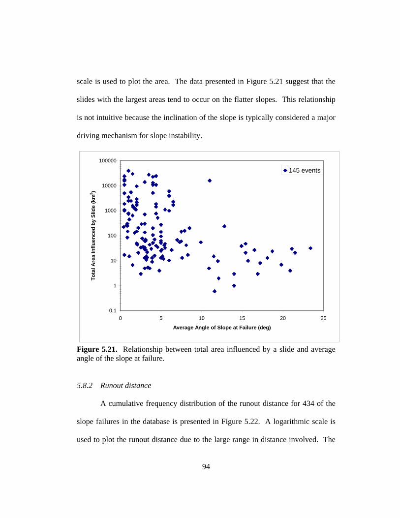
scale is used to plot the area. The data presented in Figure 5.21 suggest that the
slides with the largest areas tend to occur on the flatter slopes. This relationship
is not intuitive because the inclination of the slope is typically considered a major
driving mechanism for slope instability.
0.1
1
10
100
1000
10000
100000
0 5 10 15 20 25
Average Angle of Slope at Failure (deg)
Tota
l Are
a In
fluen
ced
by S
lide
(km
2 )
145 events
Figure 5.21. Relationship between total area influenced by a slide and average angle of the slope at failure.
5.8.2 Runout distance
A cumulative frequency distribution of the runout distance for 434 of the
slope failures in the database is presented in Figure 5.22. A logarithmic scale is
used to plot the runout distance due to the large range in distance involved. The
94
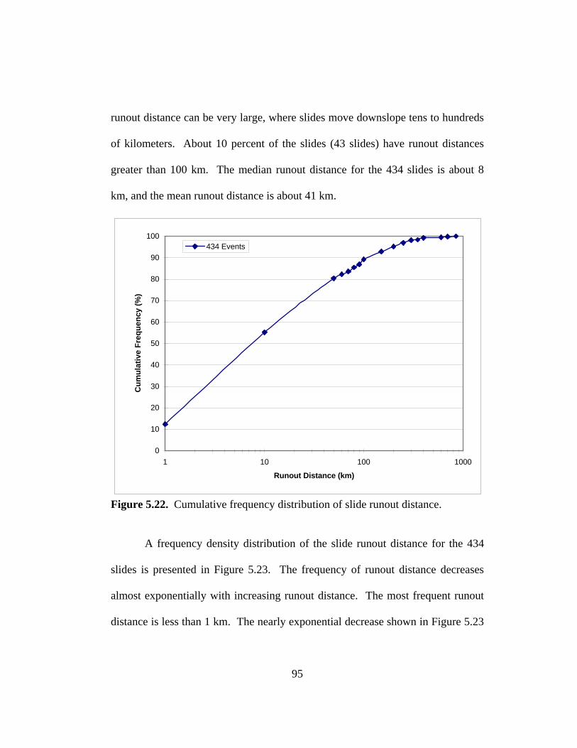
runout distance can be very large, where slides move downslope tens to hundreds
of kilometers. About 10 percent of the slides (43 slides) have runout distances
greater than 100 km. The median runout distance for the 434 slides is about 8
km, and the mean runout distance is about 41 km.
0
10
20
30
40
50
60
70
80
90
100
1 10 100 1000
Runout Distance (km)
Cum
ulat
ive
Freq
uenc
y (%
)
434 Events
Figure 5.22. Cumulative frequency distribution of slide runout distance.
A frequency density distribution of the slide runout distance for the 434
slides is presented in Figure 5.23. The frequency of runout distance decreases
almost exponentially with increasing runout distance. The most frequent runout
distance is less than 1 km. The nearly exponential decrease shown in Figure 5.23
95
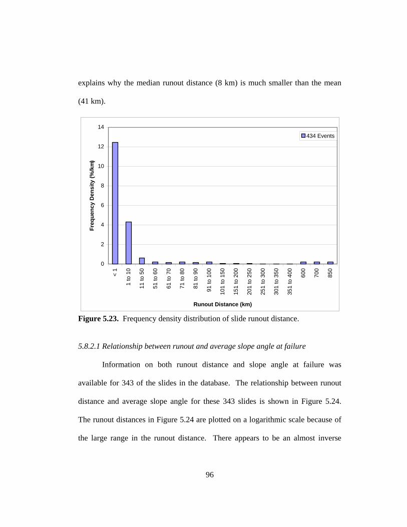
explains why the median runout distance (8 km) is much smaller than the mean
(41 km).
0
2
4
6
8
10
12
14
< 1
1 to
10
11 to
50
51 to
60
61 to
70
71 to
80
81 to
90
91 to
100
101
to 1
50
151
to 2
00
201
to 2
50
251
to 3
00
301
to 3
50
351
to 4
00 600
700
850
Runout Distance (km)
Freq
uenc
y D
ensi
ty (%
/km
)
434 Events
Figure 5.23. Frequency density distribution of slide runout distance.
5.8.2.1 Relationship between runout and average slope angle at failure
Information on both runout distance and slope angle at failure was
available for 343 of the slides in the database. The relationship between runout
distance and average slope angle for these 343 slides is shown in Figure 5.24.
The runout distances in Figure 5.24 are plotted on a logarithmic scale because of
the large range in the runout distance. There appears to be an almost inverse
96
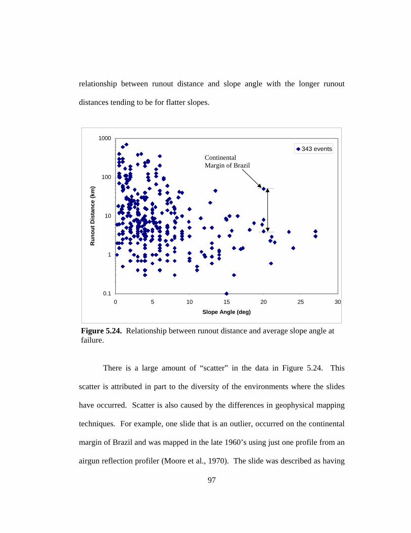
relationship between runout distance and slope angle with the longer runout
distances tending to be for flatter slopes.
0.1
1
10
100
1000
0 5 10 15 20 25 30
Slope Angle (deg)
Run
out D
ista
nce
(km
)
343 events
Continental Margin of Brazil
Figure 5.24. Relationship between runout distance and average slope angle at failure.
There is a large amount of “scatter” in the data in Figure 5.24. This
scatter is attributed in part to the diversity of the environments where the slides
have occurred. Scatter is also caused by the differences in geophysical mapping
techniques. For example, one slide that is an outlier, occurred on the continental
margin of Brazil and was mapped in the late 1960’s using just one profile from an
airgun reflection profiler (Moore et al., 1970). The slide was described as having
97
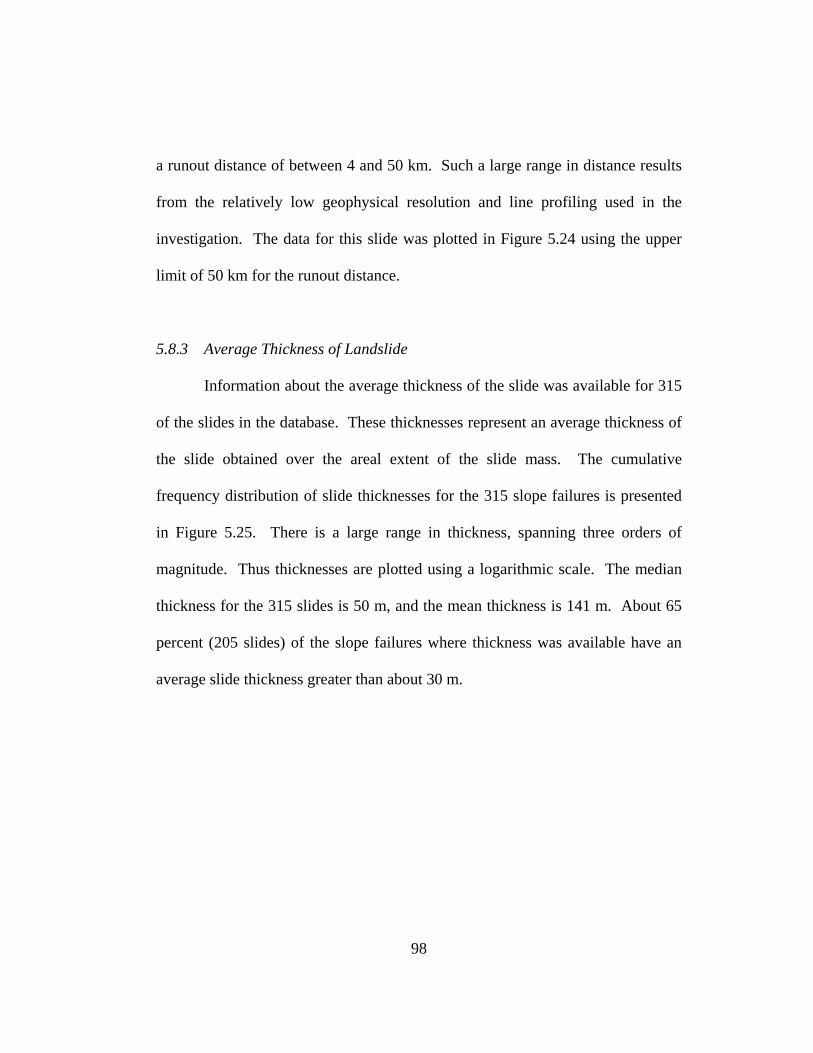
a runout distance of between 4 and 50 km. Such a large range in distance results
from the relatively low geophysical resolution and line profiling used in the
investigation. The data for this slide was plotted in Figure 5.24 using the upper
limit of 50 km for the runout distance.
5.8.3 Average Thickness of Landslide
Information about the average thickness of the slide was available for 315
of the slides in the database. These thicknesses represent an average thickness of
the slide obtained over the areal extent of the slide mass. The cumulative
frequency distribution of slide thicknesses for the 315 slope failures is presented
in Figure 5.25. There is a large range in thickness, spanning three orders of
magnitude. Thus thicknesses are plotted using a logarithmic scale. The median
thickness for the 315 slides is 50 m, and the mean thickness is 141 m. About 65
percent (205 slides) of the slope failures where thickness was available have an
average slide thickness greater than about 30 m.
98
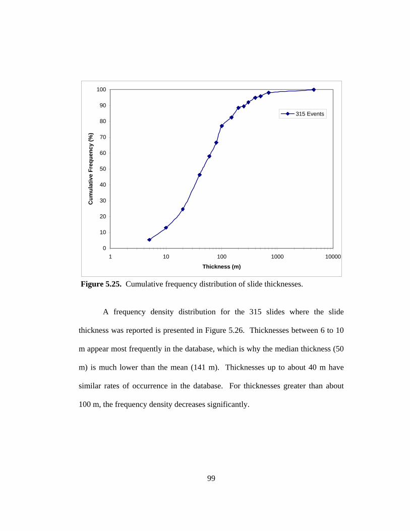
0
10
20
30
40
50
60
70
80
90
100
1 10 100 1000 10000
Thickness (m)
Cum
ulat
ive
Freq
uenc
y (%
)
315 Events
Figure 5.25. Cumulative frequency distribution of slide thicknesses.
A frequency density distribution for the 315 slides where the slide
thickness was reported is presented in Figure 5.26. Thicknesses between 6 to 10
m appear most frequently in the database, which is why the median thickness (50
m) is much lower than the mean (141 m). Thicknesses up to about 40 m have
similar rates of occurrence in the database. For thicknesses greater than about
100 m, the frequency density decreases significantly.
99
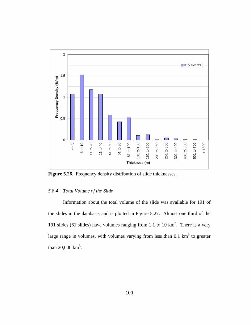
0
0.5
1
1.5
2
<= 5
6 to
10
11 to
20
21 to
40
41 to
60
61 to
80
81 to
100
101
to 1
50
151
to 2
00
201
to 2
50
251
to 3
00
301
to 4
00
401
to 5
00
501
to 7
00
> 18
00
Thickness (m)
Freq
uenc
y D
ensi
ty (%
/m)
315 events
Figure 5.26. Frequency density distribution of slide thicknesses. 5.8.4 Total Volume of the Slide
Information about the total volume of the slide was available for 191 of
the slides in the database, and is plotted in Figure 5.27. Almost one third of the
191 slides (61 slides) have volumes ranging from 1.1 to 10 km3. There is a very
large range in volumes, with volumes varying from less than 0.1 km3 to greater
than 20,000 km3.
100
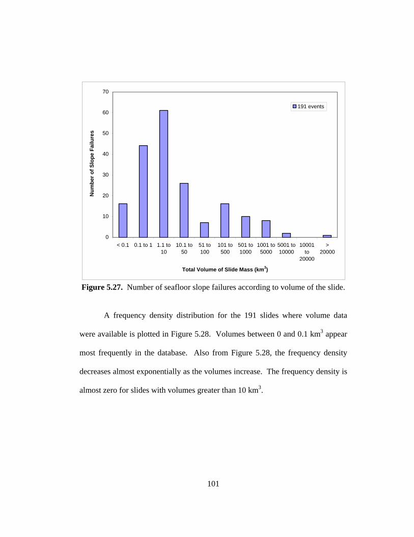
0
10
20
30
40
50
60
70
< 0.1 0.1 to 1 1.1 to10
10.1 to50
51 to100
101 to500
501 to1000
1001 to5000
5001 to10000
10001to
20000
>20000
Total Volume of Slide Mass (km3)
Num
ber o
f Slo
pe F
ailu
res
191 events
Figure 5.27. Number of seafloor slope failures according to volume of the slide.
A frequency density distribution for the 191 slides where volume data
were available is plotted in Figure 5.28. Volumes between 0 and 0.1 km3 appear
most frequently in the database. Also from Figure 5.28, the frequency density
decreases almost exponentially as the volumes increase. The frequency density is
almost zero for slides with volumes greater than 10 km3.
101
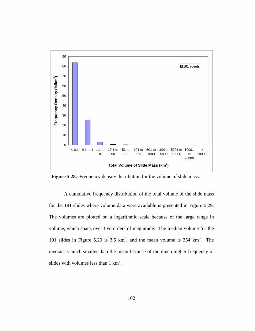
0
10
20
30
40
50
60
70
80
90
< 0.1 0.1 to 1 1.1 to10
10.1 to50
51 to100
101 to500
501 to1000
1001 to5000
5001 to10000
10001to
20000
>20000
Total Volume of Slide Mass (km3)
Freq
uenc
y D
ensi
ty (%
/km
3 )
191 events
Figure 5.28. Frequency density distribution for the volume of slide mass.
A cumulative frequency distribution of the total volume of the slide mass
for the 191 slides where volume data were available is presented in Figure 5.29.
The volumes are plotted on a logarithmic scale because of the large range in
volume, which spans over five orders of magnitude. The median volume for the
191 slides in Figure 5.29 is 3.5 km3, and the mean volume is 354 km3. The
median is much smaller than the mean because of the much higher frequency of
slides with volumes less than 1 km2.
102

0
10
20
30
40
50
60
70
80
90
100
0.1 1 10 100 1000 10000 100000
Total Volume of Slide Mass (km3)
Cum
ulat
ive
Freq
uenc
y (%
)
191 events
Figure 5.29. Cumulative frequency distribution for the volume of slide mass.
5.9 WATER DEPTHS
The shallowest water depth and deepest water depth affected by slope
failure were recorded in the database when available. There are 442 slides in the
database where the shallowest water depth affected by the slide is reported, and
408 slides where the deepest water depth affected by the slide is reported. The
shallowest water depth is reported more frequently than the deepest water depth
for two reasons: First, slope failures can extend into waters and depths beyond
where seafloor surveys have been done. Secondly, the downslope limit of the
103
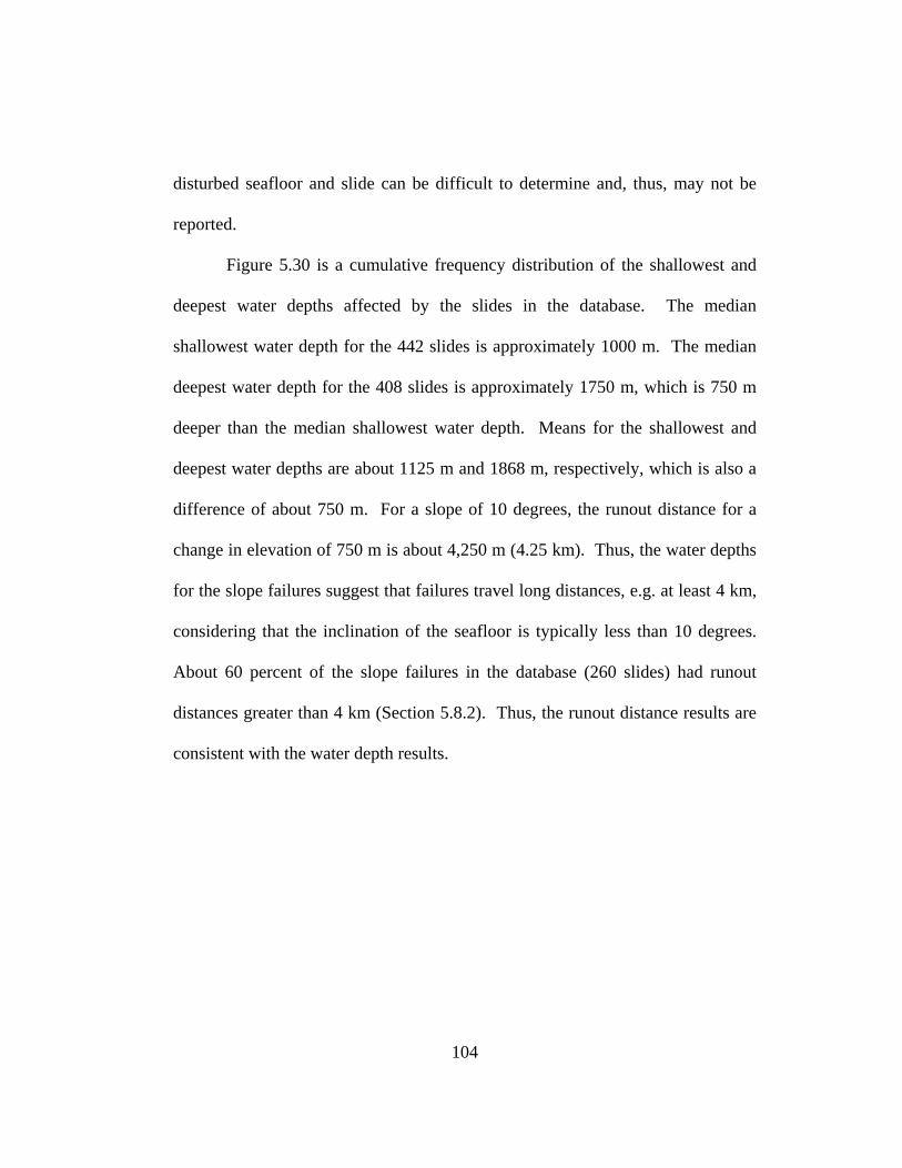
disturbed seafloor and slide can be difficult to determine and, thus, may not be
reported.
Figure 5.30 is a cumulative frequency distribution of the shallowest and
deepest water depths affected by the slides in the database. The median
shallowest water depth for the 442 slides is approximately 1000 m. The median
deepest water depth for the 408 slides is approximately 1750 m, which is 750 m
deeper than the median shallowest water depth. Means for the shallowest and
deepest water depths are about 1125 m and 1868 m, respectively, which is also a
difference of about 750 m. For a slope of 10 degrees, the runout distance for a
change in elevation of 750 m is about 4,250 m (4.25 km). Thus, the water depths
for the slope failures suggest that failures travel long distances, e.g. at least 4 km,
considering that the inclination of the seafloor is typically less than 10 degrees.
About 60 percent of the slope failures in the database (260 slides) had runout
distances greater than 4 km (Section 5.8.2). Thus, the runout distance results are
consistent with the water depth results.
104
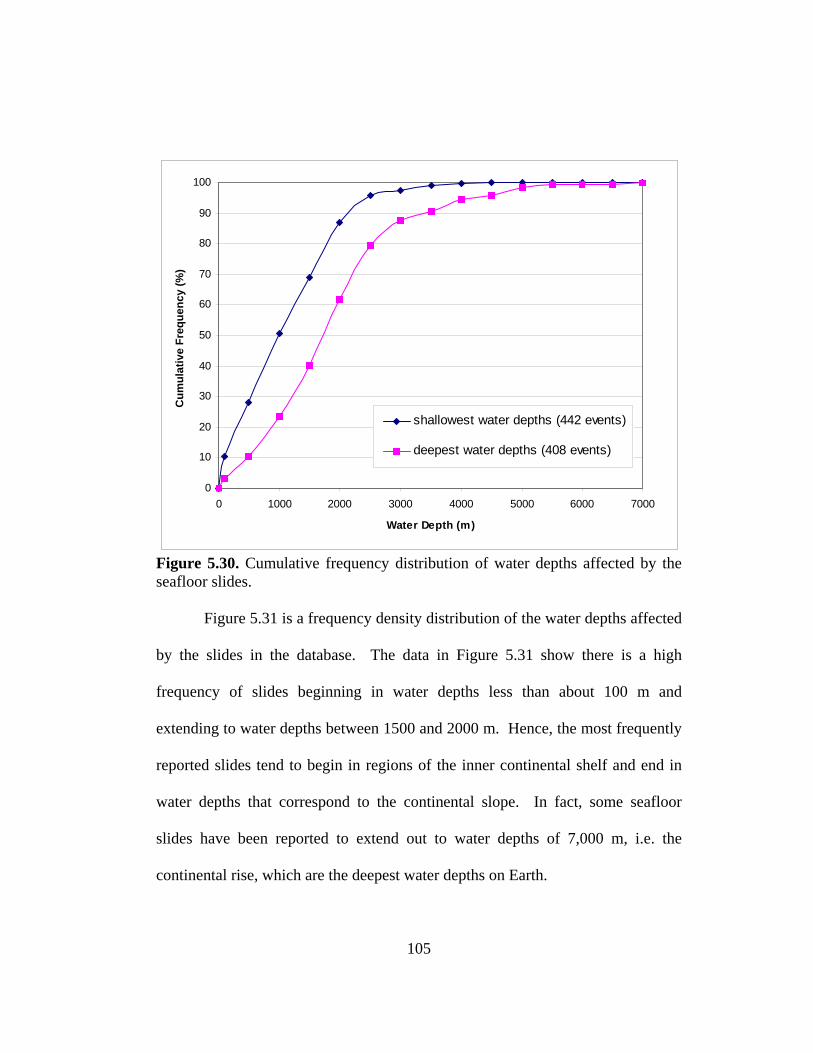
0
10
20
30
40
50
60
70
80
90
100
0 1000 2000 3000 4000 5000 6000 7000
Water Depth (m)
Cum
ulat
ive
Freq
uenc
y (%
)
shallowest water depths (442 events)
deepest water depths (408 events)
Figure 5.30. Cumulative frequency distribution of water depths affected by the seafloor slides.
Figure 5.31 is a frequency density distribution of the water depths affected
by the slides in the database. The data in Figure 5.31 show there is a high
frequency of slides beginning in water depths less than about 100 m and
extending to water depths between 1500 and 2000 m. Hence, the most frequently
reported slides tend to begin in regions of the inner continental shelf and end in
water depths that correspond to the continental slope. In fact, some seafloor
slides have been reported to extend out to water depths of 7,000 m, i.e. the
continental rise, which are the deepest water depths on Earth.
105
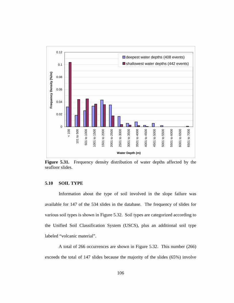
0
0.02
0.04
0.06
0.08
0.1
0.12
< 10
0
101
to 5
00
501
to 1
000
1001
to 1
500
1501
to 2
000
2001
to 2
500
2501
to 3
000
3001
to 3
500
3501
to 4
000
4001
to 4
500
4501
to 5
000
5001
to 5
500
5501
to 6
000
6001
to 6
500
6501
to 7
000
Water Depth (m)
Freq
uenc
y D
ensi
ty (%
/m)
deepest water depths (408 events)
shallowest water depths (442 events)
Figure 5.31. Frequency density distribution of water depths affected by the seafloor slides.
5.10 SOIL TYPE
Information about the type of soil involved in the slope failure was
available for 147 of the 534 slides in the database. The frequency of slides for
various soil types is shown in Figure 5.32. Soil types are categorized according to
the Unified Soil Classification System (USCS), plus an additional soil type
labeled “volcanic material”.
A total of 266 occurrences are shown in Figure 5.32. This number (266)
exceeds the total of 147 slides because the majority of the slides (65%) involve
106

more than one type of soil. This occurs because soil conditions are heterogeneous
and because submarine slides sometimes affect large areas and travel large
distances, where the slide mass passes over more than one soil type.
0
20
40
60
80
100
120
Clay Silt Sand Gravel VolcanicMaterial
Soil Type
Num
ber o
f Slo
pe F
ailu
res
Figure 5.32. The number of slope failures according to documented soil type.
The majority of the slides where information on soil type was available
involved fine-grained material, i.e. clays and silts. This characteristic is not
surprising considering that most of the Earth’s seafloor is composed of fine-
grained material, according to Lee and Mehta (1997). Furthermore, positive
excess pore water pressures can develop in marine clays and silts because of their
107
low permeability and their tendency to contract when sheared undrained; thus the
shear strength in these soils may be lower leading to slope failure.
Sixty-three (63) of the 147 events (about 43 percent) involved sandy soils.
This finding is reasonable for two reasons: First, many deltaic deposits and
material on the inner continental shelf, i.e. water depths less than about 200 m,
tend to contain coarse particles and are often classified as sands. More than 10
percent of the slides where water depths are known (about 50 slides) occurred in
shallow water regions (Section 5.9) and account for many of the slides involving
sandy soils. Secondly, earthquakes are the most common triggering mechanism
in the database (Section 5.4). Liquefaction typically occurs in saturated, loose
sandy deposits that experience earthquake shaking. Since earthquakes tend to
liquefy saturated, loose sandy soils, the fact that sandy soils appear in 43 percent
of the slides where soil data are available seems reasonable.
Gravelly soils are much less frequent than clay, silt and sand. This
probably occurs for 2 reasons: First, gravelly soils are not typically present on the
seafloor in water deeper than a few hundred meters because ocean currents cannot
transport gravelly soils large distances offshore. Thus, gravelly soils tend to be
restricted to areas near river deltas and are not generally found over other large
areas of the seafloor. The second reason why gravels are not reported for most of
the seafloor slides is that gravelly soils are less likely to experience adverse pore
water pressure conditions than other types of cohesionless soils.
108

Volcanic material is the least frequent of the soil types involved in slope
failures, probably because only a small portion of the slides in the database are
attributed to volcanic events (Section 5.4). Also, seafloor slides triggered by
volcanic activity typically did not have the soil or rock types reported.
5.11 RUNOUT CHARACTERISTICS OF SUBAQUEOUS SLIDES COMPARED TO SUBAERIAL AND QUICK CLAY SLIDES
5.11.1 INTRODUCTION
Several relationships between landslide volume and runout distance have
been developed for subaerial (Scheidegger, 1973), subaerial quick clay (Edgers
and Karlsrud, 1982) and subaqueous landslides (Edgers and Karlsrud, 1982;
Hampton et al., 1996). The findings from this previous work are summarized in
this section, and compared with data from 161 seafloor slides in the current
database.
5.11.2 SUBAERIAL SLIDES
Scheidegger (1973) addressed the runout characteristics of subaerial
slides. He expressed a “coefficient of friction” of the sliding material as H/L
where H is the difference between the highest and lowest elevations affected by
the slope failure, and L is the runout distance. Scheidegger suggested that the
ratio of H/L decreases as the volume of slide material increases. Scheidegger
109

(1973) defined a typical relationship between H/L and slide volume for subaerial
slides based on data for 33 subaerial slides, and this relationship is shown in
Figure 5.33. The solid trendline is the “average” line that was calculated by the
least squares regression method, and the dotted trendlines are one standard
deviation from the average.
H/L
Fm
5
S
s
E
igure 5.33. Ratio of height to runout distance (H/L) versus volume of slide ass for 33 subaerial slides (Scheidegger, 1973).
.11.3 SCHEIDEGGER APPROACH APPLIED TO QUICK CLAY AND SUBAQUEOUS SLIDES
Edgers and Karlsrud (1982) applied the approach developed by
cheidegger (1973) to address the runout characteristics of subaerial quick clay
lides and subaqueous slides. Hampton et al. (1996) updated the findings of
dgers and Karlsrud (1982). The relationships developed in these previous
110
studies between the ratio, H/L, and slide volume for subaerial, quick clay and
subaqueous slides are summarized in Figure 5.34. In Figure 5.34, logarithmic
scales are used for both axes because of the large range in values of the variables
involved. This figure appears in Hampton et al. (1996) and Locat and Lee (2000,
2002). The figure includes specific data points for 15 non-volcanic and 3
volcanic submarine slides. The source data of these data points is summarized in
Hampton et al. (1996).
Several trendlines are shown in Figure 5.34:
• The trendline originally proposed by Scheidegger (1973) that represents
an average for subaerial slides.
• A trendline proposed by Edgers and Karlsrud (1982) based on data for 25
submarine slides. Edgers and Karlsrud (1982) showed and stated that this
trendline represents a lower bound for the data of submarine slides, i.e. the
lowest H/L ratio, anticipated for a particular slide volume.
• A trendline proposed by Hampton et al. (1996) based on data for 15
submarine slides. Hampton et al. (1996) showed and stated that this
trendline represents an upper bound for submarine slides, i.e. the largest
H/L ratio, anticipated for a particular slide volume.
• A trendline proposed by Edgers and Karlsrud (1982) based on data for 8
quick clay slides. Edgers and Karlsrud (1982) showed and stated that this
trendline is a lower bound for subaerial quick clay slides, i.e. the lowest
111

H/L ratio, anticipated for a particular slide volume. Hampton et al. (1996)
and Locat and Lee (2002) concluded that the trendline for the subaerial
quick clay slides was a lower bound, i.e. the lowest H/L ratio, anticipated
for a particular slide volume based on data for 15 submarine slides
presented in Hampton et al. (1996).
0.0001
0.001
0.01
0.1
1
1.0E+04 1.0E+06 1.0E+08 1.0E+10 1.0E+12 1.0E+14
Volume (m3)
H/L
Nonvolcanic SlidesVolcanic SlidesAverage - Subaerial (Scheidegger, 1973)Upper bound - Submarine (Hampton et al., 1996)Lower bound - Submarine (Edgers and Karlsrud, 1982)Lower bound - Quick clay subaerial (Edgers and Karlsrud, 1982)
Figure 5.34. Ratio of height to runout distance (H/L) versus volume of slide mass (after Locat and Lee, 2002). There are suggested relationships by Scheidegger (1973), Edgers and Karlsrud (1982), and Hampton et al. (1996).
112

Edgers and Karlsrud (1982), Hampton et al. (1996), and Locat and Lee
(2000) drew four conclusions from the data shown in Figure 5.34.
1) An increase in slide volume generally corresponds with an increase in runout
distance (L) relative to the slope height (H), i.e. H/L decreases.
2) For the same volume of slide mass and the same change in elevation (H),
submarine slides tend to have larger runout distances, i.e. lower ratios of H/L,
than subaerial slides. Hampton et al. (1996) showed and stated that the
trendline for subaerial slides is an upper bound for the data of the ratio, H/L,
and slide volume of submarine landslides.
3) For the same volume of slide mass and the same change in elevation (H),
quick clay (subaerial) slides tend to have larger runout distances, i.e. lower
ratios of H/L, than submarine slides. Hampton et al. (1996) showed and
stated that the trendline for quick clay (subaerial) slides is a lower bound for
the data of the ratio, H/L, and slide volume of submarine landslides. Edgers
and Karlsrud (1982) stated that quick clay (subaerial) slides have larger
runout distances than marine soils of low to moderate sensitivity for the
following reasons:
a) the downslope gravity driving force for a subaerial slide is almost twice as
large as for a subaqueous slide.
b) there are hydrodynamic drag stresses at the top of a submarine slide due to
the overlying water, which can reduce runout.
113

c) there is greater reduction in undrained shear strength once a slide occurs
with quick clay than most marine soil, which has low to moderate
sensitivity. Locat (1995) has shown that quick clay will flow as a
Bingham fluid (Chapter 8) once failure occurs, resulting in large runout
distances on even flat slopes, i.e. low ratios of H/L.
4) Volcanic submarine slides and subaerial slides have similar runout
characteristics, i.e. the data for the ratio of H/L and volume of volcanic slides
plot in the vicinity of the subaerial trendline. Hampton et al. (1996) explain
the similarity between volcanic submarine slides and subaerial slides by
stating that volcanic slides behave much like granular rock avalanches.
Values for the ratio, H/L, and slide volume for 155 non-volcanic and 6
volcanic submarine slides from the current database are plotted in Figure 5.35.
The trendline relationships previously suggested by Edgers and Karlsrud (1982)
and Hampton et al. (1996) as respective lower and upper bounds for submarine
landslides are included in Figure 5.35.
114
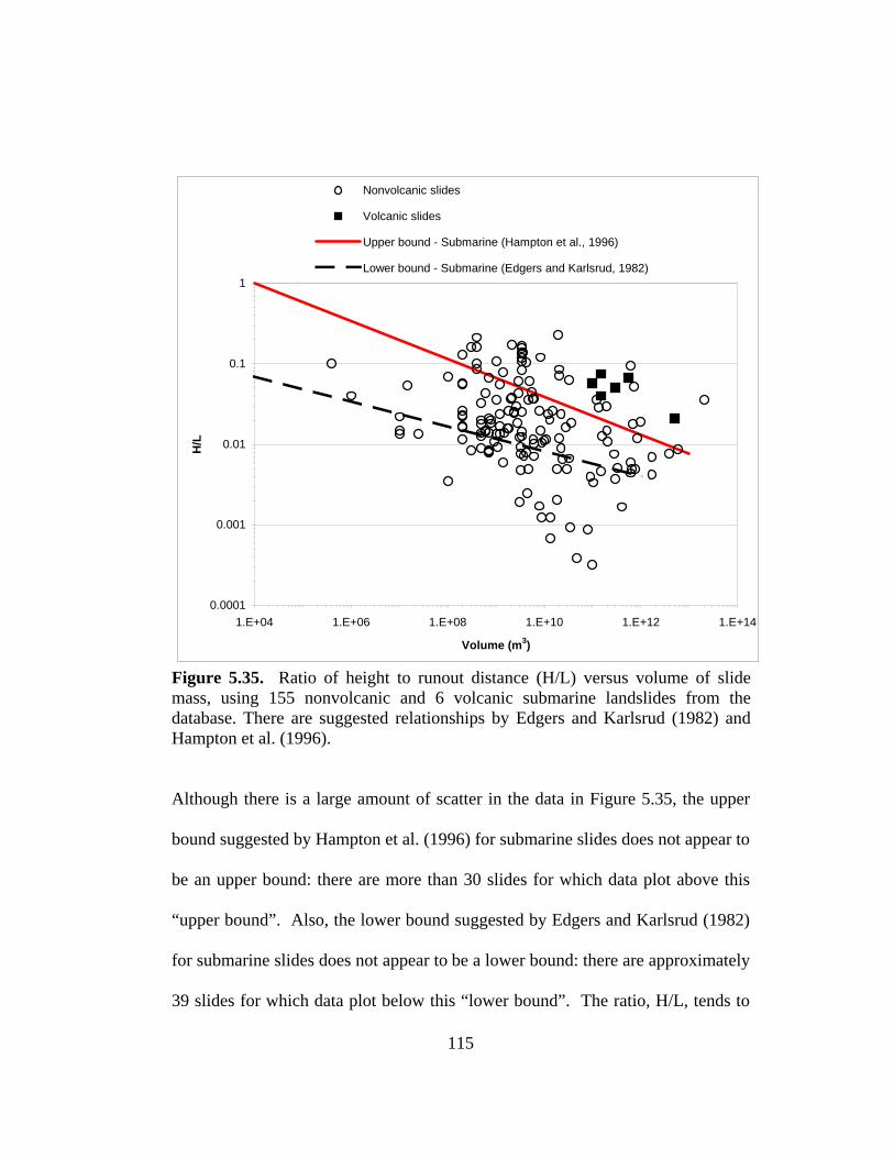
0.0001
0.001
0.01
0.1
1
1.E+04 1.E+06 1.E+08 1.E+10 1.E+12 1.E+14
Volume (m3)
H/L
Nonvolcanic slides
Volcanic slides
Upper bound - Submarine (Hampton et al., 1996)
Lower bound - Submarine (Edgers and Karlsrud, 1982)
Figure 5.35. Ratio of height to runout distance (H/L) versus volume of slide mass, using 155 nonvolcanic and 6 volcanic submarine landslides from the database. There are suggested relationships by Edgers and Karlsrud (1982) and Hampton et al. (1996).
Although there is a large amount of scatter in the data in Figure 5.35, the upper
bound suggested by Hampton et al. (1996) for submarine slides does not appear to
be an upper bound: there are more than 30 slides for which data plot above this
“upper bound”. Also, the lower bound suggested by Edgers and Karlsrud (1982)
for submarine slides does not appear to be a lower bound: there are approximately
39 slides for which data plot below this “lower bound”. The ratio, H/L, tends to
115
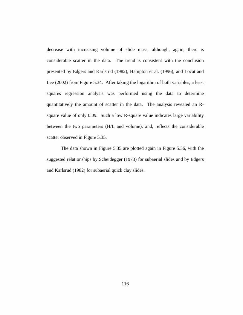
decrease with increasing volume of slide mass, although, again, there is
considerable scatter in the data. The trend is consistent with the conclusion
presented by Edgers and Karlsrud (1982), Hampton et al. (1996), and Locat and
Lee (2002) from Figure 5.34. After taking the logarithm of both variables, a least
squares regression analysis was performed using the data to determine
quantitatively the amount of scatter in the data. The analysis revealed an R-
square value of only 0.09. Such a low R-square value indicates large variability
between the two parameters (H/L and volume), and, reflects the considerable
scatter observed in Figure 5.35.
The data shown in Figure 5.35 are plotted again in Figure 5.36, with the
suggested relationships by Scheidegger (1973) for subaerial slides and by Edgers
and Karlsrud (1982) for subaerial quick clay slides.
116
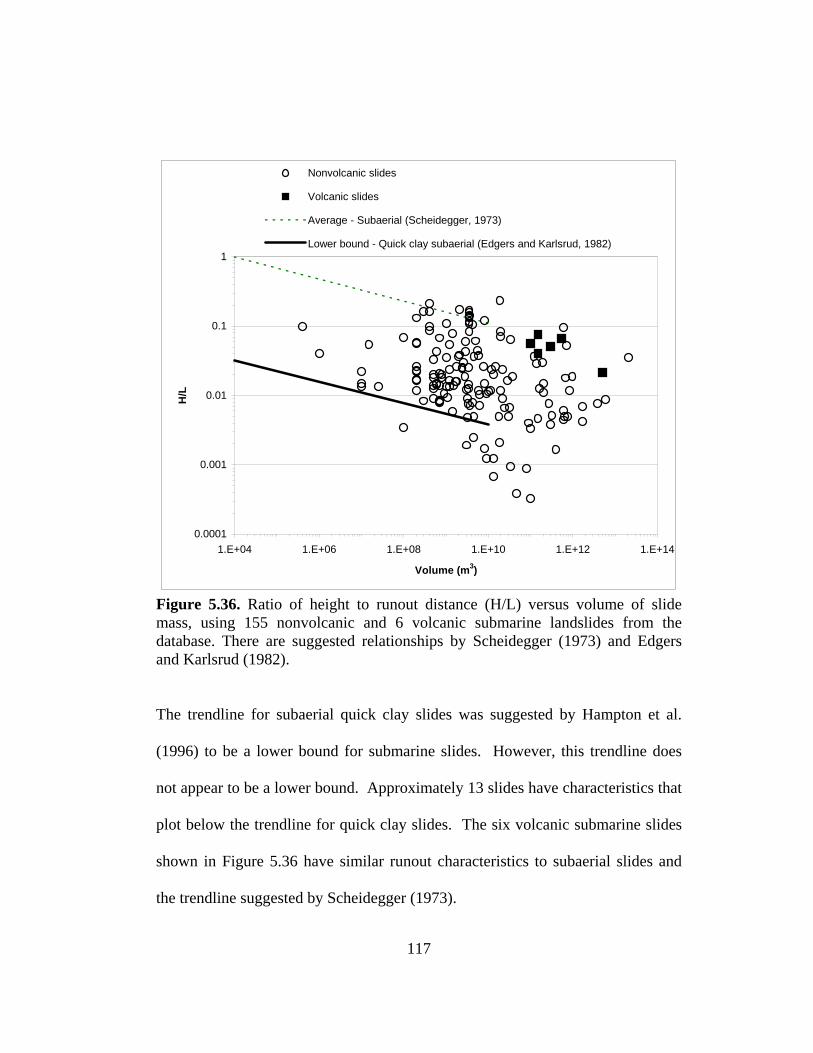
0.0001
0.001
0.01
0.1
1
1.E+04 1.E+06 1.E+08 1.E+10 1.E+12 1.E+14
Volume (m3)
H/L
Nonvolcanic slides
Volcanic slides
Average - Subaerial (Scheidegger, 1973)
Lower bound - Quick clay subaerial (Edgers and Karlsrud, 1982)
Figure 5.36. Ratio of height to runout distance (H/L) versus volume of slide mass, using 155 nonvolcanic and 6 volcanic submarine landslides from the database. There are suggested relationships by Scheidegger (1973) and Edgers and Karlsrud (1982).
The trendline for subaerial quick clay slides was suggested by Hampton et al.
(1996) to be a lower bound for submarine slides. However, this trendline does
not appear to be a lower bound. Approximately 13 slides have characteristics that
plot below the trendline for quick clay slides. The six volcanic submarine slides
shown in Figure 5.36 have similar runout characteristics to subaerial slides and
the trendline suggested by Scheidegger (1973).
117

5.12 CONCLUSIONS
There are 14 different triggering mechanisms reported in the literature,
and among these triggers, earthquakes are cited the most frequently. In terms of
certainty with regard to triggering mechanisms, only about 10 percent of the slope
failures in the database have a single, definitive trigger, and about 38 percent of
the slope failures have a completely uncertain cause of failure. The majority of
the case histories in the database (52 percent) cite several possible triggering
mechanisms.
The characteristics of runout distance, slide thickness, total area
influenced, slide volume, slope angle, and shallowest and deepest water depths
for the seafloor slope failures examined are summarized in Table 5.3. There is a
very large range between the maximum and minimum values of the
characteristics shown in Table 5.3. This is attributed to the widely varying
triggering mechanisms and soil types for submarine landslides. The median (50th
percentile) values for all the characteristics shown in Table 5.3 are smaller than
the mean values. There are two reasons for this: First, a relatively large number
of slides have small runout distances, slide thicknesses, total areas influenced,
slide volumes, slope angles and water depths, which decrease the median values
relative to the mean. Secondly, some slides have extremely large dimensions,
which increases the mean values relative to the median.
118
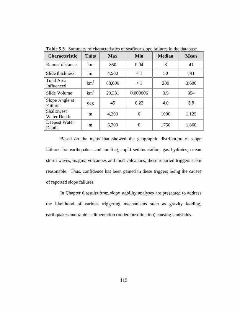
Table 5.3. Summary of characteristics of seafloor slope failures in the database. Characteristic Units Max Min Median Mean
Runout distance km 850 0.04 8 41
Slide thickness m 4,500 < 1 50 141 Total Area Influenced km2 88,000 < 1 200 3,600
Slide Volume km3 20,331 0.000006 3.5 354 Slope Angle at Failure deg 45 0.22 4.0 5.8
Shallowest Water Depth m 4,300 0 1000 1,125
Deepest Water Depth m 6,700 8 1750 1,868
Based on the maps that showed the geographic distribution of slope
failures for earthquakes and faulting, rapid sedimentation, gas hydrates, ocean
storm waves, magma volcanoes and mud volcanoes, these reported triggers seem
reasonable. Thus, confidence has been gained in these triggers being the causes
of reported slope failures.
In Chapter 6 results from slope stability analyses are presented to address
the likelihood of various triggering mechanisms such as gravity loading,
earthquakes and rapid sedimentation (underconsolidation) causing landslides.
119
CHAPTER 6
INFINITE SLOPE STABILITY ANALYSES
AND CORRELATIONS WITH SEISMICITY
6.1 INTRODUCTION
This chapter presents the results from a series of slope stability analyses
for static and pseudo-static conditions assuming an “infinite” slope. The analyses
were performed to assess the likelihood of slides being triggered by gravity,
earthquakes, and rapid sedimentation (underconsolidation), which are all common
loading conditions for seafloor slopes. The results from the pseudo-static
analyses are compared to potential seismic loads (earthquake magnitudes).
6.2 ANALYSES FOR STATIC CONDITIONS
The stability of seafloor slopes was evaluated for static conditions with
only gravity loading. To evaluate slope stability for static conditions a factor of
safety was computed. The factor of safety (F) was defined as:
τsF = (6.1)
where s is the available shear strength along a particular slip surface, and τ is the
equilibrium shear stress along the same slip surface. A slope was generally
considered stable if the factor of safety is greater than 1.0.
120
As shown in Chapter 5, many seafloor slides involve large distances
laterally in comparison to the thickness of the slide mass. For many slides, the
length of the slide is, for practical purposes, nearly infinite with respect to the
thickness of the slide. Thus, the infinite slope method is a suitable and realistic
method of analyses. Figure 6.1 shows a schematic of the geometry for an infinite
slope with a slip surface parallel to the slope face.
Specified Slip Surface
hz
l
Figure 6.1. Geometry of slope and slide mass for infinite slope failure under static conditions.
6.2.1 APPROPRIATE CONDITIONS FOR STABILITY ANALYSES
Triggers such as earthquakes, ocean waves, rapid sedimentation, rapid
erosion, and gas hydrate disassociation tend to influence a slope faster than it can
drain, and stability should be evaluated using undrained strengths. On the other
hand, triggers such as salt diapirism and faulting tend to increase gradually the
inclination of a slope, and the slope tends to be loaded at a rate slow enough to
121
allow for dissipation of excess pore water pressures and full drainage. Thus, for
these cases, stability should be evaluated using drained shear strengths. Because
failures may occur under either undrained or drained conditions, it is important
for slope stability analyses to address both.
For undrained conditions, the shear strength of the soil is usually
expressed in terms of total stresses by an equation of the form:
ϕσ tan+= cs (6.2)
where σ is the total normal stress, c is the cohesion intercept, and φ is the friction
angle. For saturated soil that is sheared undrained, the friction angle (φ) is zero,
and the undrained shear strength (su) is expressed as a “cohesion” (c).
For drained conditions, the shear strength is expressed in terms of
effective stresses by an equation of the form:
ϕσ ′′+′= tancs (6.3)
where c' and φ' are the cohesion intercept and friction angle expressed in terms of
effective stresses, respectively, and σ' is the effective normal stress. Morgenstern
(1967) and Skempton (1970) noted that many marine sediments are fine-grained,
normally consolidated to slightly overconsolidated. The cohesion (c') is typically
zero for this type of soil.
122
6.2.2 NORMALLY CONSOLIDATED SOILS
Because many marine soils tend to be normally consolidated, stability
computations were first performed for normally consolidated soils. The
undrained and drained stability of normally consolidated soils is summarized in
the following sections.
6.2.2.1 SLOPE STABILITY FOR UNDRAINED CONDITIONS
The static factor of safety for a submerged, infinite slope for undrained
conditions and total stresses was computed. The driving and resisting forces that
are imposed on a submerged, infinite slope are shown in Figure 6.2.
Specified Slip Surface
zw1
Ph
W
T
l
Pw2
Figure 6.2. Driving and resisting forces on a submerged infinite slope.
The shear stress along the slip surface for an infinite slope can be expressed as:
ββγτ sincos/ zlT ′== (6.4)
123
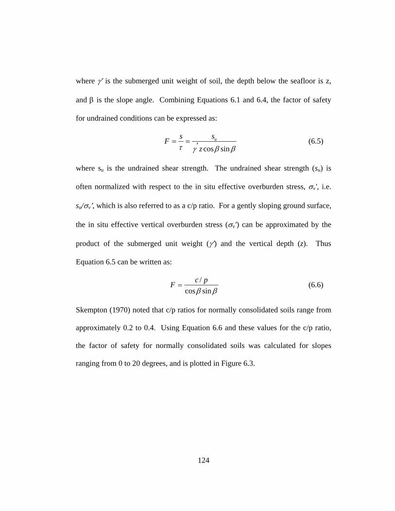
where γ′ is the submerged unit weight of soil, the depth below the seafloor is z,
and β is the slope angle. Combining Equations 6.1 and 6.4, the factor of safety
for undrained conditions can be expressed as:
ββγτ sincoszssF u
′== (6.5)
where su is the undrained shear strength. The undrained shear strength (su) is
often normalized with respect to the in situ effective overburden stress, σv', i.e.
su/σv′, which is also referred to as a c/p ratio. For a gently sloping ground surface,
the in situ effective vertical overburden stress (σv') can be approximated by the
product of the submerged unit weight (γ′) and the vertical depth (z). Thus
Equation 6.5 can be written as:
ββ sincos/ pcF = (6.6)
Skempton (1970) noted that c/p ratios for normally consolidated soils range from
approximately 0.2 to 0.4. Using Equation 6.6 and these values for the c/p ratio,
the factor of safety for normally consolidated soils was calculated for slopes
ranging from 0 to 20 degrees, and is plotted in Figure 6.3.
124
0
1
2
3
4
5
6
7
8
9
10
0 2 4 6 8 10 12 14 16 18 20
Angle of Slope, β (deg)
Fact
or o
f Saf
ety
0.20.30.4
c/p ratios:
Figure 6.3. Variation in factor of safety with slope angle for infinite slope in normally consolidated soils using undrained shear strengths.
Most slope failures in the database (334 slides) occurred in slopes inclined
at angles flatter than about 10 degrees. In order for such slopes to fail under static
conditions (F < 1), the c/p ratio would need to be less than 0.17 as shown in
Figure 6.4. If 0.20 represents a lower limit for the c/p ratio, there must have been
a trigger other than gravity to cause most of the offshore slopes flatter than 10
degrees to fail.
125
6.2.2.2 SLOPE STABILITY FOR DRAINED CONDITIONS
Stability calculations for drained conditions were performed using shear
strengths expressed in terms of effective stresses. The cohesion (c') was assumed
to be zero, which is the case for many normally consolidated soils. The static
factor of safety (F) for an infinite slope with no water flow and a cohesion of zero
is expressed as:
βϕ
tantan ′
=F (6.7)
Based on this equation, slope failures (F < 1) are expected to occur when the
slope angle (β) is greater than the friction angle expressed in terms of effective
stresses (φ'). Most slope failures in the database (334 slides) occurred in slopes
inclined at angles flatter than about 10 degrees. The effective stress friction angle
(φ′) for many fine-grained soils is expected to be at least 20 degrees, according to
Terzaghi et al. (1996). For example, for the 15 slopes in the database where
effective stress friction angles were reported, the friction angles were all greater
than 20 degrees. For most slopes in the database, the slope angle is less than the
effective stress friction angle and slope failure (F < 1) is not expected. Therefore,
failure of normally consolidated soil slopes caused only by gravity loads cannot
be explained for drained conditions.
126
6.2.3 EFFECTIVE STRESS ANALYSES OF UNDERCONSOLIDATED SOILS
Some offshore slopes contain underconsolidated soils. For example, rapid
sedimentation, the second most common trigger identified in the database, tends
to generate excess pore water pressures in most underconsolidated marine soils.
Many river deltas experience rapid sedimentation where the soils tend to be
underconsolidated. Thus, the stability of underconsolidated soils is of interest and
is examined in this section.
The infinite slope method was used to back calculate excess pore water
pressures required to cause slope failure assuming a slope in underconsolidated
soil. The effective cohesion (c') was assumed to be zero, and the shear strength
along the slip surface (s) was evaluated in terms of effective stresses. In this case,
the factor of safety (F) is computed from:
ββγφβγ
τ sincostan)cos( 2
zuzsF
′′−′
== (6.8)
where ū is the excess pore water pressure. By rearranging Equation 6.8, the
excess pore water pressure gradient required to trigger failure (F = 1) was
computed from:
ϕββϕβ
γ ′−′
=′ tansincostancos2
z
u (6.9)
where ū/γ´z is excess pore water pressure gradient. The excess pore water
pressure gradient was considered to be linear with depth below the seafloor when
127

computing Equation 6.9. The excess pore water pressure gradient was calculated
for various slope angles and effective stress friction angles, φ′, and is plotted in
Figure 6.4. The shaded region in Figure 6.4 indicates the gradients that would be
required to trigger slides for most of the slopes in the database, i.e. β ≤ 10º and φ′
≥ 20º.
0.0
0.1
0.2
0.3
0.4
0.5
0.6
0.7
0.8
0.9
1.0
0 2 4 6 8 10 12 14 16 18 20
Slope Angle, β
Exce
ss p
ore
wat
er p
ress
ure
grad
ient
101520253035
φ ' (deg)
Figure 6.4. Excess pore water pressure gradients required for failure of an infinite slope for various slopes angles and friction angles (c′ = 0).
Referring to this shaded region, excess pore water pressures greater than about 50
percent of the vertical effective stress would be required to trigger failure.
128

Bennett et al. (1976) have reported underconsolidated soils in the Mississippi
River delta as having large excess pore water pressures (ū ≥ 0.5σv′), yet these
soils were on very flat slopes. Because such large excess pore water pressures
can be developed, the above analyses indicate that underconsolidated soils are
typically not stable under static gravity loads in slopes inclined at angles greater
than 10 degrees.
6.2.4 SUMMARY OF ANALYSES FOR STATIC CONDITIONS
The static slope stability analyses of normally consolidated soils suggested
that most seafloor slides are not likely caused by gravity loads alone. Thus, for
most slopes in the database, apart from underconsolidated soils, a trigger other
than gravity must have caused slope failure.
For underconsolidated soils, excess pore water pressures greater than
about 50 percent of the vertical effective stress were shown to be required for
failure in slopes inclined at angles flatter than 10 degrees. Since excess pore
water pressures of this magnitude can be developed, it was inferred that these
soils are typically not stable when inclined at angles greater than 10 degrees.
6.3 ANALYSES FOR PSEUDO-STATIC CONDITIONS
The most common triggering mechanism indicated in the database is
earthquake loading, and, thus, it was deemed important to evaluate how
129
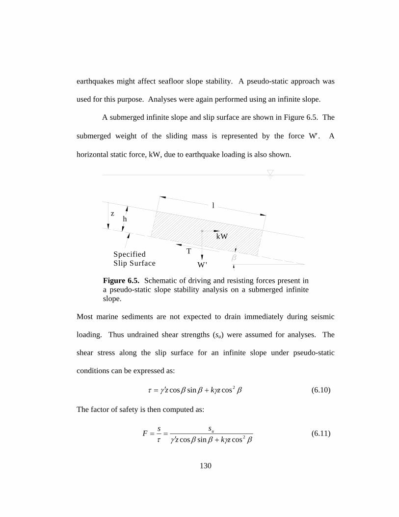
earthquakes might affect seafloor slope stability. A pseudo-static approach was
used for this purpose. Analyses were again performed using an infinite slope.
A submerged infinite slope and slip surface are shown in Figure 6.5. The
submerged weight of the sliding mass is represented by the force W′. A
horizontal static force, kW, due to earthquake loading is also shown.
Specified Slip Surface
zh
W'
kW
T
l
Figure 6.5. Schematic of driving and resisting forces present in a pseudo-static slope stability analysis on a submerged infinite slope.
Most marine sediments are not expected to drain immediately during seismic
loading. Thus undrained shear strengths (su) were assumed for analyses. The
shear stress along the slip surface for an infinite slope under pseudo-static
conditions can be expressed as:
βγββγτ 2cossincos zkz +′= (6.10)
The factor of safety is then computed as:
βγββγτ 2cossincos zkzssF u
+′== (6.11)
130
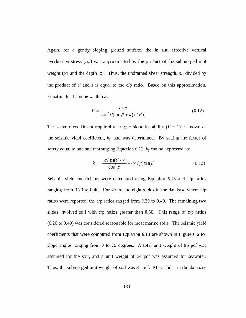
Again, for a gently sloping ground surface, the in situ effective vertical
overburden stress (σv') was approximated by the product of the submerged unit
weight (γ′) and the depth (z). Thus, the undrained shear strength, su, divided by
the product of γ′ and z is equal to the c/p ratio. Based on this approximation,
Equation 6.11 can be written as:
)]/([tancos/
2 γγββ ′+=
kpcF (6.12)
The seismic coefficient required to trigger slope instability (F = 1) is known as
the seismic yield coefficient, ky, and was determined. By setting the factor of
safety equal to one and rearranging Equation 6.12, ky can be expressed as:
βγγβ
γγ tan)/(cos
)/)(/(2
′−′
=pcky (6.13)
Seismic yield coefficients were calculated using Equation 6.13 and c/p ratios
ranging from 0.20 to 0.40. For six of the eight slides in the database where c/p
ratios were reported, the c/p ratios ranged from 0.20 to 0.40. The remaining two
slides involved soil with c/p ratios greater than 0.50. This range of c/p ratios
(0.20 to 0.40) was considered reasonable for most marine soils. The seismic yield
coefficients that were computed from Equation 6.13 are shown in Figure 6.6 for
slope angles ranging from 0 to 20 degrees. A total unit weight of 95 pcf was
assumed for the soil, and a unit weight of 64 pcf was assumed for seawater.
Thus, the submerged unit weight of soil was 31 pcf. Most slides in the database
131
(334 slides) occurred on slopes flatter than about 10 degrees. This range of slope
angles and the probable range of c/p ratios is represented by the shaded region in
Figure 6.6. The seismic yield coefficients (ky) for the shaded region are 0.13 or
less. In the next section, the seismic conditions required to induce permanent
deformation and possibly slope failure will be evaluated and compared with the
seismic conditions from several slides in the database.
0.00
0.02
0.04
0.06
0.08
0.10
0.12
0.14
0 2 4 6 8 10 12 14 16 18 20
Slope Angle, β (deg)
Seis
mic
Yie
ld C
oeff
icie
nt, k
y (g)
0.200.250.300.350.40
c/p ratios:
Figure 6.6. Seismic yield coefficients required for failure of a submerged infinite slope for various slope angles and c/p ratios.
132
6.4 CORRELATION OF RESULTS FROM PSEUDO-STATIC ANALYSES WITH SEISMICITY
In order to evaluate the feasibility of earthquakes as a trigger, a series of
analyses of seismic conditions required to induce permanent deformations in a
seafloor slope were conducted. The procedures used and results are presented in
this section. Seismic loading can be represented by the maximum acceleration in
a soil deposit, kmax, that is a function of the input ground motion and the geometry
of the sliding mass. For this study, the input ground motion was assumed to be
the peak ground acceleration in the underlying bedrock, PGAROCK, induced by an
earthquake. The geometry of the sliding mass was assumed to be an “infinite”
slope.
The Hynes and Franklin (1984) criterion was used as a conservative
screening method for permanent displacements in a slope. The upper bound
results from Hynes and Franklin’s Newmark rigid sliding block analyses of 348
earthquake ground motions assuming one meter of displacement yielded a ratio of
ky to kmax (ky/kmax) of about 0.17. Also, their criterion yielded an amplification
factor, kmax/PGAROCK, of about 3.0, and resulted in a seismic yield coefficient of
one half of the peak ground acceleration in rock, i.e. ky/PGAROCK = 0.17 * 3.0 ≈
0.5. The pseudo-static analyses in Section 6.3 showed that the largest seismic
yield coefficient (ky) assuming probable conditions of shear strength and slope
angle based on the database is about 0.13. Thus, PGAROCK values of at least 0.26
133
g would cause permanent deformation in a slope that has a seismic yield
coefficient of 0.13 or less. To determine the seismic conditions required to
produce these PGAROCK values (at least 0.26 g), the following analyses were
performed.
6.4.1 ATTENUATION RELATIONSHIPS
The attenuation relationships developed by Abrahamson and Silva (1997)
were used to determine specific seismic conditions of earthquake magnitude and
distance between the earthquake (source) and the slope (site) that would induce a
value of PGAROCK of at least 0.26 g. Abrahamson and Silva (1997) developed
attenuation relationships for estimating peak ground accelerations based on the
type of fault, earthquake magnitude, and distance between the source and site.
These attenuation relationships were based on empirical site responses from a
database of 655 recordings from 58 earthquakes. These attenuation relationships
for estimating PGAROCK are generally consistent with other methods developed
by Seed and Idriss (1982) and Boore, Joyner, and Fumal (1997).
From the attenuation relationships developed by Abrahamson and Silva
(1997), a regression model was used to obtain PGAROCK as a function of
earthquake magnitude and distance between the source and site. The value of
PGAROCK was assumed by Abrahamson and Silva (1997) to be the spectral
acceleration, Sa, at a period (time) of 0.01 seconds. The general function of the
134
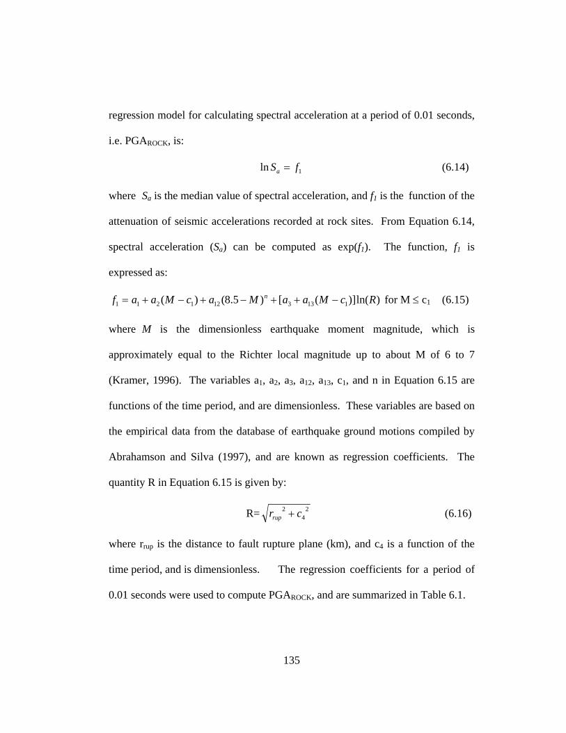
regression model for calculating spectral acceleration at a period of 0.01 seconds,
i.e. PGAROCK, is:
1ln fSa = (6.14)
where Sa is the median value of spectral acceleration, and f1 is the function of the
attenuation of seismic accelerations recorded at rock sites. From Equation 6.14,
spectral acceleration (Sa) can be computed as exp(f1). The function, f1 is
expressed as:
)ln()]([)5.8()( 1133121211 RcMaaMacMaaf n −++−+−+= for M ≤ c1 (6.15)
where M is the dimensionless earthquake moment magnitude, which is
approximately equal to the Richter local magnitude up to about M of 6 to 7
(Kramer, 1996). The variables a1, a2, a3, a12, a13, c1, and n in Equation 6.15 are
functions of the time period, and are dimensionless. These variables are based on
the empirical data from the database of earthquake ground motions compiled by
Abrahamson and Silva (1997), and are known as regression coefficients. The
quantity R in Equation 6.15 is given by:
R= 24
2 crrup + (6.16)
where rrup is the distance to fault rupture plane (km), and c4 is a function of the
time period, and is dimensionless. The regression coefficients for a period of
0.01 seconds were used to compute PGAROCK, and are summarized in Table 6.1.
135
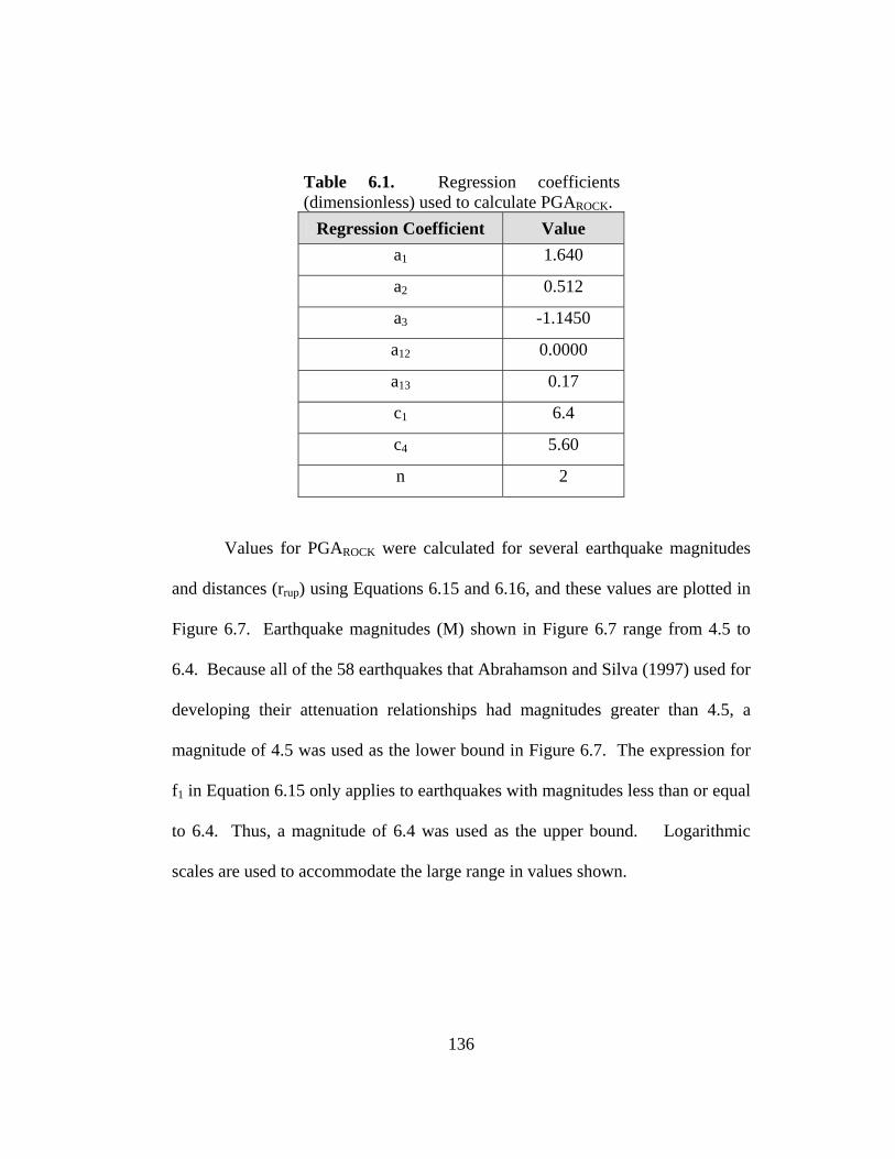
Table 6.1. Regression coefficients (dimensionless) used to calculate PGAROCK.
Regression Coefficient Value a1 1.640
a2 0.512
a3 -1.1450
a12 0.0000
a13 0.17
c1 6.4
c4 5.60
n 2
Values for PGAROCK were calculated for several earthquake magnitudes
and distances (rrup) using Equations 6.15 and 6.16, and these values are plotted in
Figure 6.7. Earthquake magnitudes (M) shown in Figure 6.7 range from 4.5 to
6.4. Because all of the 58 earthquakes that Abrahamson and Silva (1997) used for
developing their attenuation relationships had magnitudes greater than 4.5, a
magnitude of 4.5 was used as the lower bound in Figure 6.7. The expression for
f1 in Equation 6.15 only applies to earthquakes with magnitudes less than or equal
to 6.4. Thus, a magnitude of 6.4 was used as the upper bound. Logarithmic
scales are used to accommodate the large range in values shown.
136
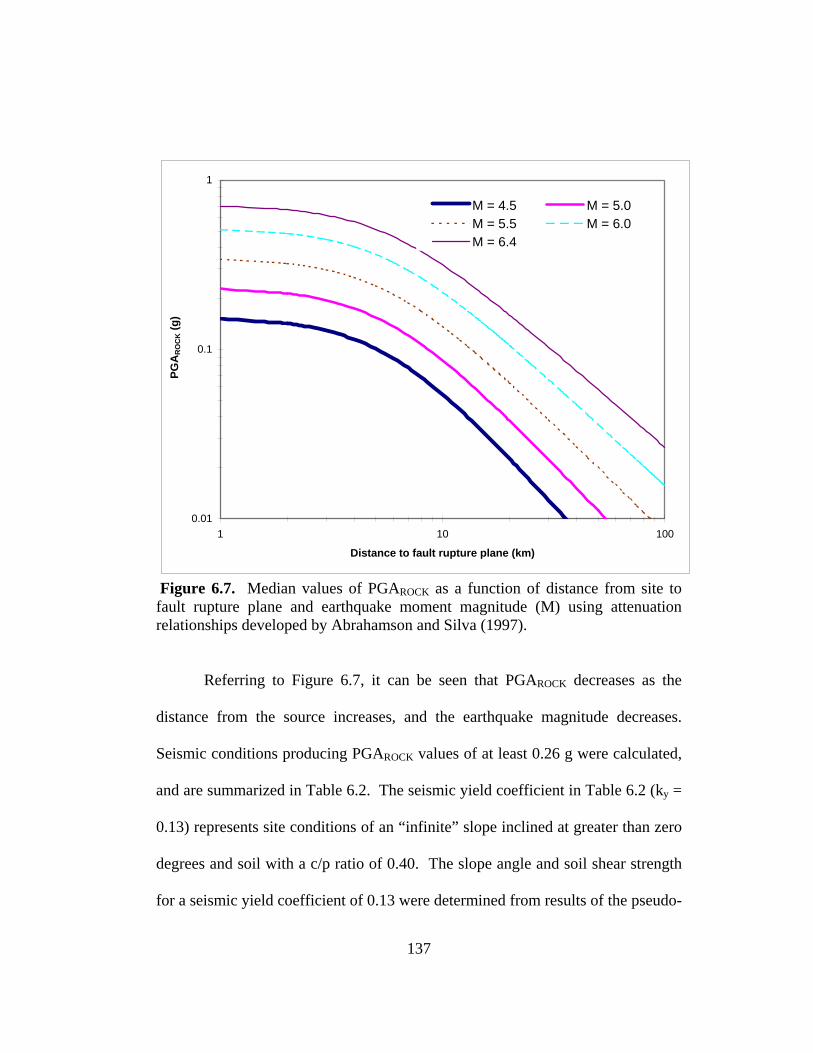
0.01
0.1
1
1 10 100
Distance to fault rupture plane (km)
PGA
RO
CK (g
)
M = 4.5 M = 5.0M = 5.5 M = 6.0M = 6.4
Figure 6.7. Median values of PGAROCK as a function of distance from site to fault rupture plane and earthquake moment magnitude (M) using attenuation relationships developed by Abrahamson and Silva (1997).
Referring to Figure 6.7, it can be seen that PGAROCK decreases as the
distance from the source increases, and the earthquake magnitude decreases.
Seismic conditions producing PGAROCK values of at least 0.26 g were calculated,
and are summarized in Table 6.2. The seismic yield coefficient in Table 6.2 (ky =
0.13) represents site conditions of an “infinite” slope inclined at greater than zero
degrees and soil with a c/p ratio of 0.40. The slope angle and soil shear strength
for a seismic yield coefficient of 0.13 were determined from results of the pseudo-
137
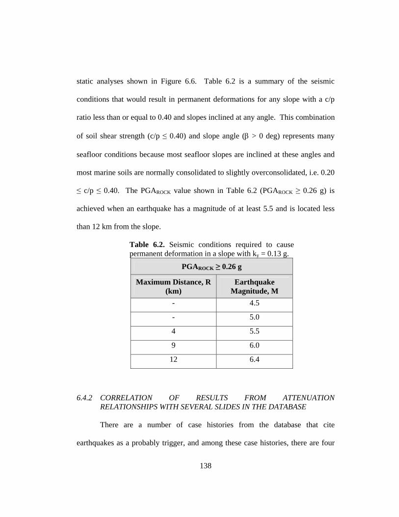
static analyses shown in Figure 6.6. Table 6.2 is a summary of the seismic
conditions that would result in permanent deformations for any slope with a c/p
ratio less than or equal to 0.40 and slopes inclined at any angle. This combination
of soil shear strength (c/p ≤ 0.40) and slope angle (β > 0 deg) represents many
seafloor conditions because most seafloor slopes are inclined at these angles and
most marine soils are normally consolidated to slightly overconsolidated, i.e. 0.20
≤ c/p ≤ 0.40. The PGAROCK value shown in Table 6.2 (PGAROCK ≥ 0.26 g) is
achieved when an earthquake has a magnitude of at least 5.5 and is located less
than 12 km from the slope.
Table 6.2. Seismic conditions required to cause permanent deformation in a slope with ky = 0.13 g.
PGAROCK ≥ 0.26 g
Maximum Distance, R (km)
Earthquake Magnitude, M
- 4.5
- 5.0
4 5.5
9 6.0
12 6.4
6.4.2 CORRELATION OF RESULTS FROM ATTENUATION
RELATIONSHIPS WITH SEVERAL SLIDES IN THE DATABASE
There are a number of case histories from the database that cite
earthquakes as a probably trigger, and among these case histories, there are four
138
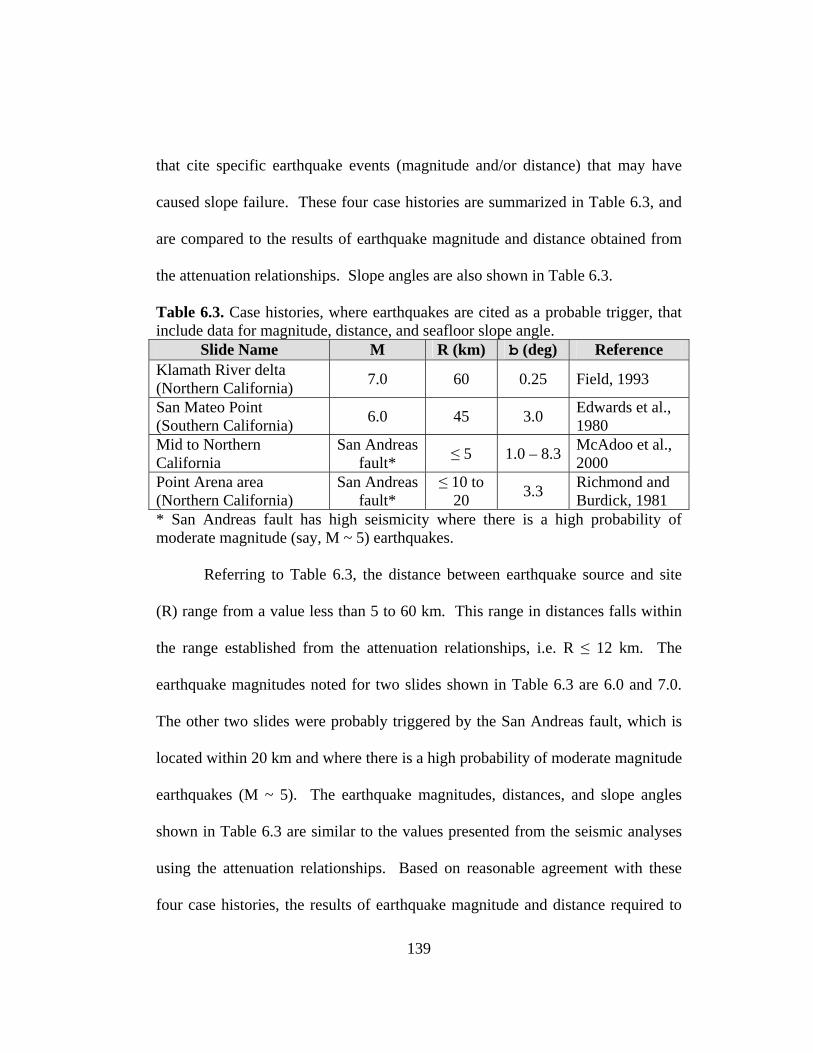
that cite specific earthquake events (magnitude and/or distance) that may have
caused slope failure. These four case histories are summarized in Table 6.3, and
are compared to the results of earthquake magnitude and distance obtained from
the attenuation relationships. Slope angles are also shown in Table 6.3.
Table 6.3. Case histories, where earthquakes are cited as a probable trigger, that include data for magnitude, distance, and seafloor slope angle.
Slide Name M R (km) b (deg) Reference Klamath River delta (Northern California) 7.0 60 0.25 Field, 1993
San Mateo Point (Southern California) 6.0 45 3.0 Edwards et al.,
1980 Mid to Northern California
San Andreas fault* ≤ 5 1.0 – 8.3 McAdoo et al.,
2000 Point Arena area (Northern California)
San Andreas fault*
≤ 10 to 20 3.3 Richmond and
Burdick, 1981 * San Andreas fault has high seismicity where there is a high probability of moderate magnitude (say, M ~ 5) earthquakes.
Referring to Table 6.3, the distance between earthquake source and site
(R) range from a value less than 5 to 60 km. This range in distances falls within
the range established from the attenuation relationships, i.e. R ≤ 12 km. The
earthquake magnitudes noted for two slides shown in Table 6.3 are 6.0 and 7.0.
The other two slides were probably triggered by the San Andreas fault, which is
located within 20 km and where there is a high probability of moderate magnitude
earthquakes (M ~ 5). The earthquake magnitudes, distances, and slope angles
shown in Table 6.3 are similar to the values presented from the seismic analyses
using the attenuation relationships. Based on reasonable agreement with these
four case histories, the results of earthquake magnitude and distance required to
139

cause slope deformation and possible failure, which were obtained from the
seismic analyses, are considered to be realistic.
6.5 CONCLUSIONS
The analyses of slope stability and seismicity presented in this chapter
addressed the likelihood of slides being triggered by gravity, rapid sedimentation
(underconsolidation), and earthquakes. Several conclusions can be drawn from
the analyses:
1) It seems unlikely that most of the slope failures in the database in
normally consolidated and overconsolidated soils were caused by gravity
loads alone considering the slope angles and probable drained and
undrained shear strengths.
2) Rapid sedimentation can produce underconsolidated soils with strengths
low enough for gravity sliding to occur on slopes as flat as one degree,
which includes many of the slopes in the database.
3) For slopes located less than about 12 km from an earthquake of magnitude
5.5 or greater, slope failures are likely to occur. These values of
earthquake magnitude and distance are considered realistic because they
are in reasonable agreement with four slides examined in the database.
Now that the cause of seafloor slope failure has been examined, mechanisms of
slope movement after initial failure are addressed in the following chapters.
140

CHAPTER 7
HYDROPLANING MECHANISM
7.1 INTRODUCTION
Hydroplaning may explain why many submarine slides have the large
runout distances that were shown in Chapter 5. Experimental evidence of
hydroplaning has been presented by Mohrig et al. (1998, 1999), Harff et al.
(1998), and Laval et al. (1988). This work is examined in this chapter, and where
appropriate, results derived from the experimental studies are applied to slides in
the database. In addition, a simple sliding block model was developed for this
thesis, and is presented to illustrate how the conditions necessary for
hydroplaning might be achieved.
7.2 DEFINITION OF HYDROPLANING
Hydroplaning occurs when a layer of fluid becomes entrapped between a
sliding soil mass and the underlying soil. The layer of fluid significantly reduces
the resistance between the moving soil mass and the underlying soil.
When a subaqueous flow advances through a body of water, a fluid
pressure in excess of hydrostatic pressure is induced at the front of the sliding
mass by the moving body as shown in Figure 7.1. A measure of the pressure is
the fluid stagnation pressure, pf, which is expressed as:
141
2
2vp wf
ρ= (7.1)
where ρw is the mass density of water (1.94 slugs/ft3 ≅ 1.00 x 10³ kg/m3), and
v is the velocity of the sliding mass. This fluid pressure is hydrodynamic and
depends on the velocity of the sliding mass. The excess fluid pressure
developed on a moving soil mass acts from the stagnation point, shown as “s”
in Figure 7.1, down to the supporting surface of the slide mass. The fluid
pressure is resisted by an equivalent downward normal stress, pd, produced by
the submerged weight of the slide mass on the slope. The downward normal
stress is related to a pressure, pd, expressed as:
βρρ cos)( awdd ghp −= (7.2)
where ρd is the total mass density of the soil, and g is the acceleration due to
gravity (32.2 ft/s2 ≅ 9.8 m/s2). The term ha represents the average slide
thickness, and β is the slope angle.
142

Sliding Mass
Supporting Surface
az h
f
A
Fluid Pressure, p
s
Debris Flow Pressure, p
d
g
Figure 7.1. Fluid and debris flow pressures that are generated at the front of a sliding mass. “s” indicates stagnation point, above which there are no hydrodynamic pressures. “A” is the location where hydroplaning is initiated.
Hydroplaning occurs when the hydrodynamic pressure, which is
proportional to pf, exceeds the downward normal stress, which is related to pd.
The point at which hydroplaning is initiated is labeled as “A” in Figure 7.1.
7.3 OVERVIEW OF PAST EXPERIMENTS
Mohrig et al. (1998, 1999), Harff et al. (1998), and Laval et al. (1988)
performed experiments to study hydroplaning of subaqueous slides. Mohrig et
al. performed two sets of experiments (1998, 1999). Both experiments were
performed on soil submerged in water where the soil moved down an inclined
channel, thus creating subaqueous landslides or debris flows that were confined
143
by the sidewalls of the channel. Harff et al. (1998) performed unconfined flow
experiments where soil submerged in water slid down an inclined channel and
exited into a tank, simulating a debris flow exiting a submarine canyon onto an
open slope. Harff et al. (1998) inferred that hydroplaning of subaqueous slides
occurred because their observations were consistent with Mohrig et al.’s (1998,
1999) observations of slides where hydroplaning was actually observed. Mohrig
et al.’s and Harff et al.’s observations will be described later in this chapter.
Laval et al. (1988) performed experiments with sandy soil that was submerged in
water. In Laval et al.’s experiments, the soil was allowed to flow down an
inclined channel and resulted in subaqueous turbidity currents that were confined
by the sidewalls of the channel. Laval et al.’s (1988) experiments were carried
out with low density “sand flows” using various water-saline solutions, where the
density of the sand was only about 1.2 to 1.3 times the density of water. Laval et
al. observed a thin layer of fluid trapped between the advancing “sand flow” and
the channel, and concluded that the flowing mass was hydroplaning.
Mohrig et al.’s (1998, 1999) experiments provide the most compelling and
comprehensive support of hydroplaning among all of these experiments. In the
following sections, their work is examined and their results are applied to data for
the submarine slides in the database.
144

7.4 MOHRIG ET AL.’S (1998, 1999) EXPERIMENTS
The experiments of Mohrig et al. (1998, 1999) are summarized in this
section. The discussion includes description of their apparatus, soil conditions,
measurements, results, observations of hydroplaning, and general characteristics
of slides where hydroplaning occurs.
7.4.1 APPARATUS
The setup for Mohrig et al.’s (1998, 1999) two sets of experiments
consisted of a glass-walled tank that was 10 m long, 3 m high and 0.6 m wide. A
rectangular channel, 0.2 m in width, was suspended in the tank as shown
schematically by the cross-section in Figure 7.2. The soil was continuously
mixed in a “head tank”, and then fed into the channel through a “debris feed
point” as shown in Figures 7.2 and 7.3. The tank was referred to as a “head tank”
because it was located at the entrance to the channel.
145

3.0 m
0.6 m
0.2 m
glass-walled tank
rectangular channel
debris feed point
head tank
Figure 7.2. Cross section (A-A´) of experimental apparatus used by Mohrig et al. (1998, 1999).
A profile view of the experimental facility is shown in Figure 7.3. The
channel had two segments and was fabricated so that each segment could be
inclined at different angles. The lengths of the upper and lower segments were
5.7 m and 4.3 m, respectively. There was a gap located between the upper and
lower segments so that the debris flow, which moved as a fluid-like mass, could
exit the channel through a vent, as shown in Figure 7.3. A second vent was
146
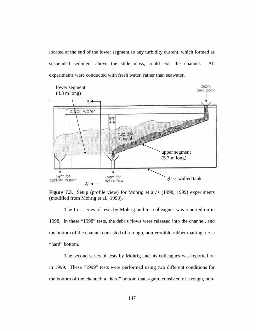
located at the end of the lower segment so any turbidity current, which formed as
suspended sediment above the slide mass, could exit the channel. All
experiments were conducted with fresh water, rather than seawater.
lower segment (4.3 m long)
A
A´ Figure 7.3. Setup (profile view) for Mohrig et al.’s(modified from Mohrig et al., 1998). The first series of tests by Mohrig and his col
1998. In these “1998” tests, the debris flows were rel
the bottom of the channel consisted of a rough, non-ero
“hard” bottom.
The second series of tests by Mohrig and his
in 1999. These “1999” tests were performed using t
the bottom of the channel: a “hard” bottom that, again
147
upper segment (5.7 m long)
glass-walled tank
(1998, 1999) experiments
leagues was reported on in
eased into the channel, and
dible rubber matting, i.e. a
colleagues was reported on
wo different conditions for
, consisted of a rough, non-
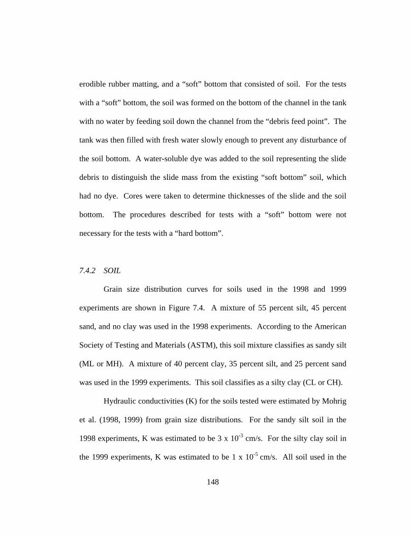
erodible rubber matting, and a “soft” bottom that consisted of soil. For the tests
with a “soft” bottom, the soil was formed on the bottom of the channel in the tank
with no water by feeding soil down the channel from the “debris feed point”. The
tank was then filled with fresh water slowly enough to prevent any disturbance of
the soil bottom. A water-soluble dye was added to the soil representing the slide
debris to distinguish the slide mass from the existing “soft bottom” soil, which
had no dye. Cores were taken to determine thicknesses of the slide and the soil
bottom. The procedures described for tests with a “soft” bottom were not
necessary for the tests with a “hard bottom”.
7.4.2 SOIL
Grain size distribution curves for soils used in the 1998 and 1999
experiments are shown in Figure 7.4. A mixture of 55 percent silt, 45 percent
sand, and no clay was used in the 1998 experiments. According to the American
Society of Testing and Materials (ASTM), this soil mixture classifies as sandy silt
(ML or MH). A mixture of 40 percent clay, 35 percent silt, and 25 percent sand
was used in the 1999 experiments. This soil classifies as a silty clay (CL or CH).
Hydraulic conductivities (K) for the soils tested were estimated by Mohrig
et al. (1998, 1999) from grain size distributions. For the sandy silt soil in the
1998 experiments, K was estimated to be 3 x 10⁻³ cm/s. For the silty clay soil in
the 1999 experiments, K was estimated to be 1 x 10⁻⁵ cm/s. All soil used in the
148
tests was deposited as a slurry after being mixed in the head tank prior to being
released into the channel. The soil was not compacted or densified, and no time
was allowed for consolidation. The gravimetric water content of the soil was
measured in the head tank prior to being released in the channel. The water
content of the soil for the 1998 experiments was 16.5 percent, and was 39 percent
for the 1999 experiments.
0
10
20
30
40
50
60
70
80
90
100
0.0010.010.11Grain Size (mm)
Cum
ulat
ive
Perc
ent P
assi
ng (%
)
1998 experiments
1999 experiments
SAND SILT
#200
CLAY
Figure 7.4. Grain size distributions for soil used in the experiments (obtained from dry weight and particle size data presented in Mohrig et al. 1998, 1999).
The dye that was used in the 1999 tests affected the consistency and
rheology of the slurry. Accordingly, three consistencies of slurry were observed
149
and described. Mohrig et al. described these as “sticky”, “medium” and “runny”.
The slurry described as “sticky” had the least amount of dye, and had the highest
yield strength, τy, and viscosity, µs. The slurry described as “medium” had a
moderate amount of dye, and a lower yield strength and viscosity than the
“sticky” slurry. The slurry described as “runny” had the most amount of dye, and
the lowest yield strength and viscosity.
7.4.3 MEASUREMENTS
For the 1998 and 1999 series of tests, slope angles of the channel
segments were measured. For the 1998 tests, the upper segment was inclined at
angles ranging from 1 to 20 degrees, and the lower segment was horizontal. For
the 1999 tests, the upper segment was fixed at 6 degrees, and the lower segment
was inclined at 1 degree.
For both tests (1998, 1999), video cameras recorded the slide motion. For
the 1998 tests, a single video camera was attached to a moving carriage and
followed the slide as it moved down the channel. For the 1999 tests, eight fixed
video cameras were used, with each camera mounted on one of the eight panels of
glass that made up the outer tank. Analysis of the video camera recordings
allowed velocities to be determined. The “frontal” or “head” velocity represented
the velocity at the front of the debris flow.
150
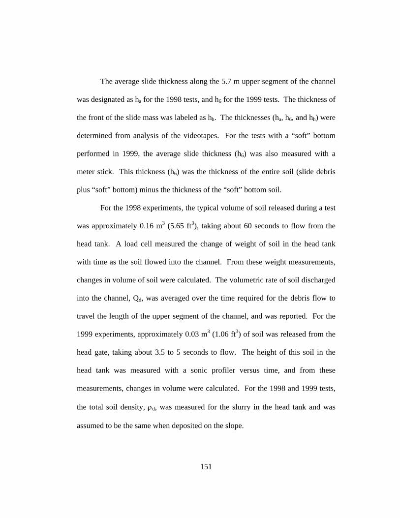
The average slide thickness along the 5.7 m upper segment of the channel
was designated as ha for the 1998 tests, and h6 for the 1999 tests. The thickness of
the front of the slide mass was labeled as hh. The thicknesses (ha, h6, and hh) were
determined from analysis of the videotapes. For the tests with a “soft” bottom
performed in 1999, the average slide thickness (h6) was also measured with a
meter stick. This thickness (h6) was the thickness of the entire soil (slide debris
plus “soft” bottom) minus the thickness of the “soft” bottom soil.
For the 1998 experiments, the typical volume of soil released during a test
was approximately 0.16 m3 (5.65 ft3), taking about 60 seconds to flow from the
head tank. A load cell measured the change of weight of soil in the head tank
with time as the soil flowed into the channel. From these weight measurements,
changes in volume of soil were calculated. The volumetric rate of soil discharged
into the channel, Qd, was averaged over the time required for the debris flow to
travel the length of the upper segment of the channel, and was reported. For the
1999 experiments, approximately 0.03 m3 (1.06 ft3) of soil was released from the
head gate, taking about 3.5 to 5 seconds to flow. The height of this soil in the
head tank was measured with a sonic profiler versus time, and from these
measurements, changes in volume were calculated. For the 1998 and 1999 tests,
the total soil density, ρd, was measured for the slurry in the head tank and was
assumed to be the same when deposited on the slope.
151

7.4.4 RESULTS
Results for ten of the 1998 tests were reported by Mohrig et al. (1998),
and are summarized in Table 7.1. The results in Table 7.1 include the test
number, slope angle, total dry density of the soil, average rate of volume
discharge, average slide thickness, debris head thickness, front velocity, and
“characteristic average velocity”. The characteristic average velocity, v*, of the
slide is defined as the velocity at which the debris is supplied to the channel, and
is expressed as:
a
d
WhQv =* (7.3)
where W is the width of the channel in meters, ha is the average slide thickness in
millimeters, and Qd is the average volumetric rate of soil discharged into the
channel (l/s).
152
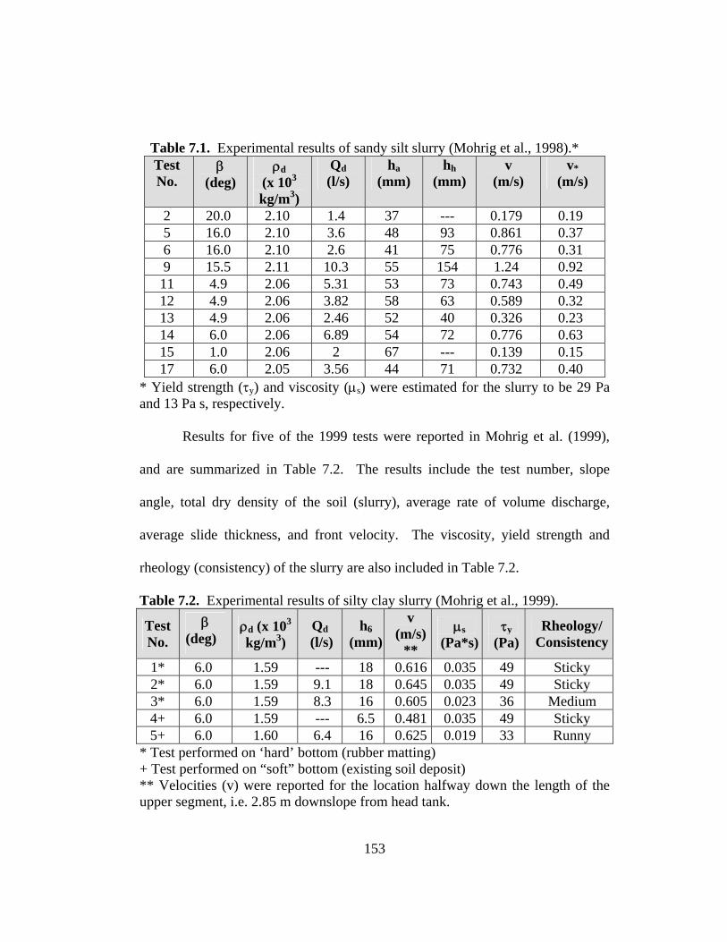
Table 7.1. Experimental results of sandy silt slurry (Mohrig et al., 1998).* Test No.
β (deg)
ρd(x 103 kg/m3)
Qd (l/s)
ha(mm)
hh(mm)
v (m/s)
v*(m/s)
2 20.0 2.10 1.4 37 --- 0.179 0.19 5 16.0 2.10 3.6 48 93 0.861 0.37 6 16.0 2.10 2.6 41 75 0.776 0.31 9 15.5 2.11 10.3 55 154 1.24 0.92 11 4.9 2.06 5.31 53 73 0.743 0.49 12 4.9 2.06 3.82 58 63 0.589 0.32 13 4.9 2.06 2.46 52 40 0.326 0.23 14 6.0 2.06 6.89 54 72 0.776 0.63 15 1.0 2.06 2 67 --- 0.139 0.15 17 6.0 2.05 3.56 44 71 0.732 0.40
* Yield strength (τy) and viscosity (µs) were estimated for the slurry to be 29 Pa and 13 Pa s, respectively.
Results for five of the 1999 tests were reported in Mohrig et al. (1999),
and are summarized in Table 7.2. The results include the test number, slope
angle, total dry density of the soil (slurry), average rate of volume discharge,
average slide thickness, and front velocity. The viscosity, yield strength and
rheology (consistency) of the slurry are also included in Table 7.2.
Table 7.2. Experimental results of silty clay slurry (Mohrig et al., 1999).
Test No.
β (deg)
ρd (x 103 kg/m3)
Qd (l/s)
h6 (mm)
v (m/s)
**
µs (Pa*s)
τy (Pa)
Rheology/ Consistency
1* 6.0 1.59 --- 18 0.616 0.035 49 Sticky 2* 6.0 1.59 9.1 18 0.645 0.035 49 Sticky 3* 6.0 1.59 8.3 16 0.605 0.023 36 Medium 4+ 6.0 1.59 --- 6.5 0.481 0.035 49 Sticky 5+ 6.0 1.60 6.4 16 0.625 0.019 33 Runny
* Test performed on ‘hard’ bottom (rubber matting) + Test performed on “soft” bottom (existing soil deposit) ** Velocities (v) were reported for the location halfway down the length of the upper segment, i.e. 2.85 m downslope from head tank.
153
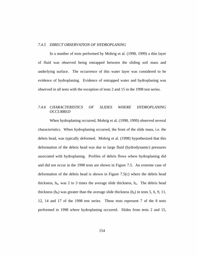
7.4.5 DIRECT OBSERVATION OF HYDROPLANING
In a number of tests performed by Mohrig et al. (1998, 1999) a thin layer
of fluid was observed being entrapped between the sliding soil mass and
underlying surface. The occurrence of this water layer was considered to be
evidence of hydroplaning. Evidence of entrapped water and hydroplaning was
observed in all tests with the exception of tests 2 and 15 in the 1998 test series.
7.4.6 CHARACTERISTICS OF SLIDES WHERE HYDROPLANING OCCURRED
When hydroplaning occurred, Mohrig et al. (1998, 1999) observed several
characteristics. When hydroplaning occurred, the front of the slide mass, i.e. the
debris head, was typically deformed. Mohrig et al. (1998) hypothesized that this
deformation of the debris head was due to large fluid (hydrodynamic) pressures
associated with hydroplaning. Profiles of debris flows where hydroplaning did
and did not occur in the 1998 tests are shown in Figure 7.5. An extreme case of
deformation of the debris head is shown in Figure 7.5(c) where the debris head
thickness, hh, was 2 to 3 times the average slide thickness, ha. The debris head
thickness (hh) was greater than the average slide thickness (ha) in tests 5, 6, 9, 11,
12, 14 and 17 of the 1998 test series. These tests represent 7 of the 8 tests
performed in 1998 where hydroplaning occurred. Slides from tests 2 and 15,
154
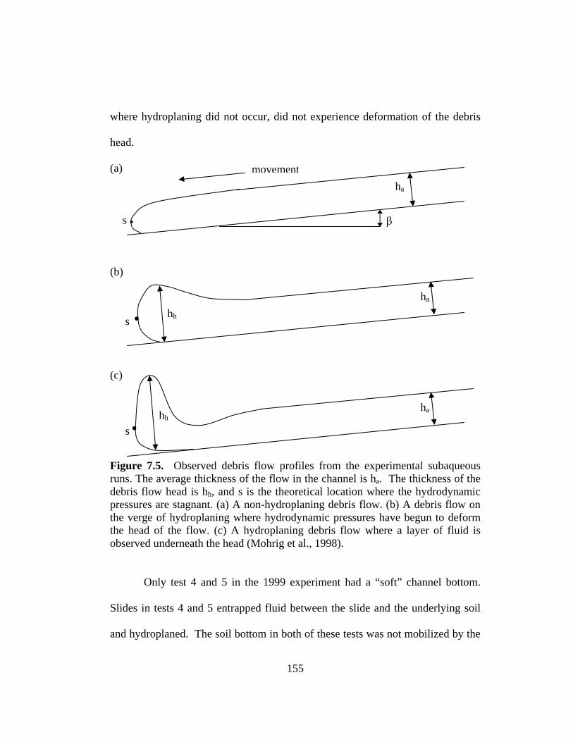
where hydroplaning did not occur, did not experience deformation of the debris
head.
(a)
(b)
(c)
s
s .
t
. s hh
. hh
Figure 7.5. Observed debrisruns. The average thickness ofdebris flow head is hh, and s pressures are stagnant. (a) A nthe verge of hydroplaning whthe head of the flow. (c) A hobserved underneath the head
Only test 4 and 5 in t
Slides in tests 4 and 5 entrapp
and hydroplaned. The soil bo
movemen
β
ha
ha
ha
flow profiles from the experimental subaqueous the flow in the channel is ha. The thickness of the is the theoretical location where the hydrodynamic on-hydroplaning debris flow. (b) A debris flow on ere hydrodynamic pressures have begun to deform ydroplaning debris flow where a layer of fluid is (Mohrig et al., 1998).
he 1999 experiment had a “soft” channel bottom.
ed fluid between the slide and the underlying soil
ttom in both of these tests was not mobilized by the
155
passing debris flows, i.e. the existing soil deposits were not disturbed by the
slides. Mohrig et al. hypothesized that the thin layer of water prevented
significant shear stresses and corresponding strains from being transmitted to the
seafloor.
Among all of the slides where hydroplaning occurred in the 1998 test
series (tests 5, 6, 9, 11, 12, 13, 14 and 17), the frontal velocities (v) exceeded the
calculated characteristic average velocities (v*) as shown in Table 7.1. Slides in
tests 2 and 15, which did not entrap fluid between the slide and the underlying
soil and, thus, where hydroplaning did not occur, had frontal velocities that were
less than the calculated characteristic average velocities.
For the 1999 experiments, the frontal velocity of the slide was plotted
versus downslope distance from the head gate, and is shown in Figure 7.6. The
channel bottom condition for each test (“soft” or “hard”), the slurry consistency
(“sticky”, “medium”, or “runny”), and the slope angles of the upper and lower
segments of the channel are also shown in Figure 7.6. Runout distances of the
five tests were about the same, regardless of the differing channel bottom (“soft”
versus “hard”) and slurry consistencies. Frontal velocities from the five tests are
approximately constant beginning about 2 m downslope from the head gate, and
remain so until the bottom slope angle changes about 6 m downslope, regardless
of the channel bottom (“soft” versus “hard”) and slurry consistency. The
velocities are similar, becoming about 55 to 60 cm/s at the end of the 6 deg slope.
156

Mohrig et al. (1999) hypothesized that the thin layer of water entrapped due to
hydroplaning accounted for the very similar velocity profiles and runout distances
among the five slides that have different soil and channel bottom conditions.
Thus, Mohrig et al. (1999) also hypothesized that hydroplaning is a mechanism
for large runout distances that is independent of rheology.
Location of the head gate
Tests with a “hard” channel bottom
Velocities reported in Table 7.2
Slurry Rheology Slides 1, 2 and 4: “Sticky” Slide 3: “Medium” Slide 5: “Runny”
Tests with a “schannel bottom
Figure 7.6. Velocity ofMohrig et al. (1999) erheology, and location (modified from Mohrig e
oft”
6 d
the fxperimof vet al., 1
1 deg slope eg slope
ront of slide versus downslope distance for the ents. Bottom of channel conditions, slurry
locities reported in Table 7.2 are also noted 999).
157
7.5 HYPOTHESIS OF HYDROPLANING OF SEAFLOOR SLIDES BASED ON GEOPHYSICAL IMAGERY
For a slide where hydroplaning occurs, the head of the debris flow can
deform, as was shown in Figure 7.5 (c). Mohrig et al. (1998) and Harff et al.
(1998) observed in the laboratory an extreme case of the profile illustrated in
Figure 7.5 (c), where the debris head actually becomes completely detached from
the rest of the flow. Mohrig et al. and Harff et al. hypothesized that the head of
the debris flow becomes detached due to the large hydrodynamic pressures
associated with hydroplaning, and the detached head then accelerates on the
entrapped layer of fluid ahead of the remainder of the debris flow. There is also
natural landslide evidence to support separation and detachment of a debris flow
like those observed in the laboratory. Two seafloor slides, Alika debris avalanche
in Hawaii (Lipman et al., 1988; Normark et al., 1993) and Kitimat Inlet in British
Columbia (Prior et al., 1984; Johns et al., 1986), provide examples where the head
of a debris flow detached from the rest of the flow. A three-dimensional
illustration of the Kitimat Inlet landslide is shown in Figure 7.7. In this figure,
blocks of sediment, labeled as outrunner blocks, are shown at the furthest
downslope location in the mass movement. Prior et al. (1984) hypothesized that
the outrunner blocks are heads of debris flows that detached from the rest of the
flows due to hydroplaning.
158

Figure 7.7. Interpretive three-dimensional image of the Kitimat Inlet landslide in British Columbia (Prior et al., 1984). The outrunner blocks are hypothesized to be heads of debris flows that detached from the rest of the flows due to hydroplaning. 7.6 DENSIMETRIC FROUDE NUMBER: INDICATOR OF
HYDROPLANING BASED ON EXPERIMENTAL RESULTS
Mohrig et al. (1998) observed that there was a relationship between the
“densimetric Froude number”, Frd, and the occurrence of hydroplaning. The
densimetric Froude number is a dimensionless parameter that has been used to
characterize gravity-dominated flow involving two “liquids” of slightly different
densities, and is expressed as:
159
⎟⎟⎠
⎞⎜⎜⎝
⎛ ∆=
ρρgL
vFrd (7.4)
where ∆ρ is the difference in density between the two fluids, ρ is the density of
one of the fluids, and L is the downslope distance traveled. Using the variables
from their experiments, Mohrig et al. (1998) modified Equation 7.4 to the form:
( ) ⎟⎟⎠
⎞⎜⎜⎝
⎛−
=
1cosw
da
d
gh
vFr
ρρβ
(7.5)
Mohrig et al. (1998, 1999) calculated densimetric Froude numbers for
their tests. The results are summarized in Table 7.3 in order of increasing
densimetric Froude number, and are presented along with the experimental
parameters used for the calculations.
160
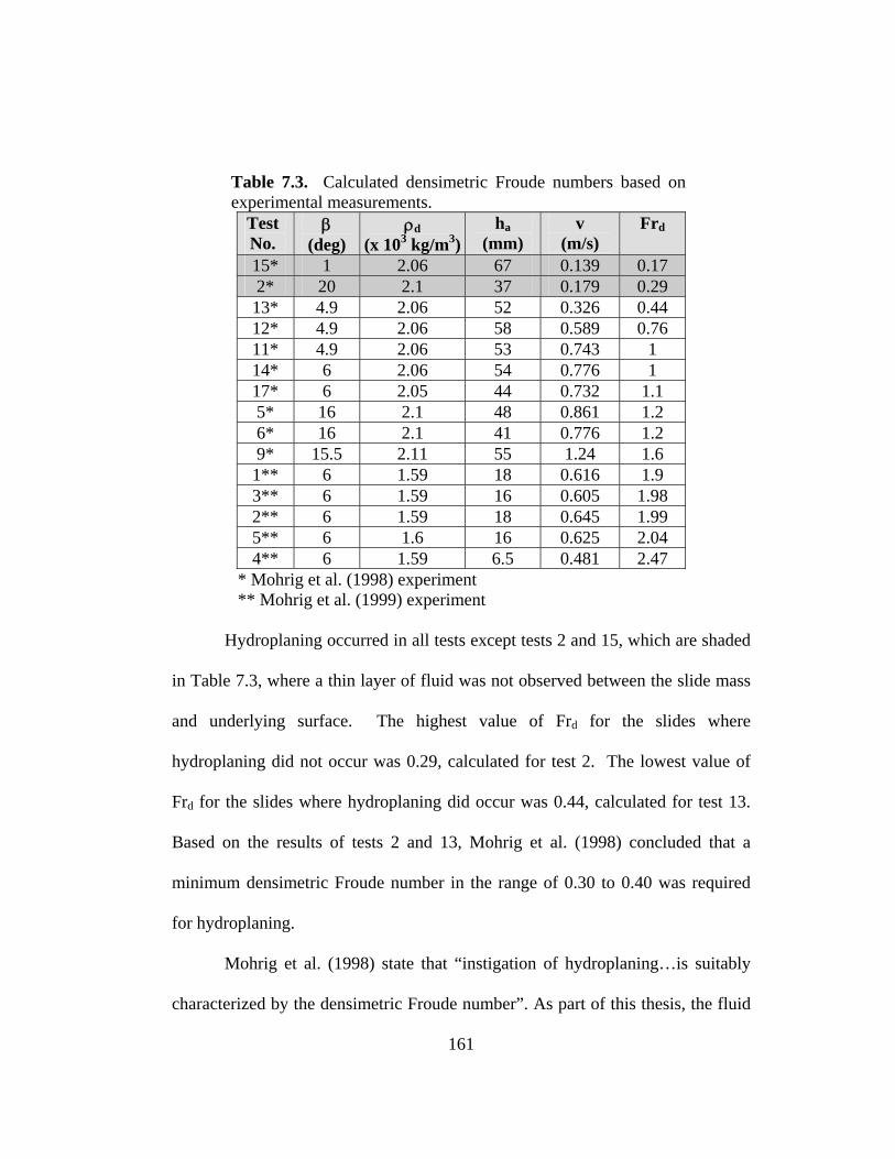
Table 7.3. Calculated densimetric Froude numbers based on experimental measurements.
Test No.
β (deg)
ρd(x 103 kg/m3)
ha(mm)
v (m/s)
Frd
15* 1 2.06 67 0.139 0.17 2* 20 2.1 37 0.179 0.29 13* 4.9 2.06 52 0.326 0.44 12* 4.9 2.06 58 0.589 0.76 11* 4.9 2.06 53 0.743 1 14* 6 2.06 54 0.776 1 17* 6 2.05 44 0.732 1.1 5* 16 2.1 48 0.861 1.2 6* 16 2.1 41 0.776 1.2 9* 15.5 2.11 55 1.24 1.6 1** 6 1.59 18 0.616 1.9 3** 6 1.59 16 0.605 1.98 2** 6 1.59 18 0.645 1.99 5** 6 1.6 16 0.625 2.04 4** 6 1.59 6.5 0.481 2.47
* Mohrig et al. (1998) experiment ** Mohrig et al. (1999) experiment
Hydroplaning occurred in all tests except tests 2 and 15, which are shaded
in Table 7.3, where a thin layer of fluid was not observed between the slide mass
and underlying surface. The highest value of Frd for the slides where
hydroplaning did not occur was 0.29, calculated for test 2. The lowest value of
Frd for the slides where hydroplaning did occur was 0.44, calculated for test 13.
Based on the results of tests 2 and 13, Mohrig et al. (1998) concluded that a
minimum densimetric Froude number in the range of 0.30 to 0.40 was required
for hydroplaning.
Mohrig et al. (1998) state that “instigation of hydroplaning…is suitably
characterized by the densimetric Froude number”. As part of this thesis, the fluid
161
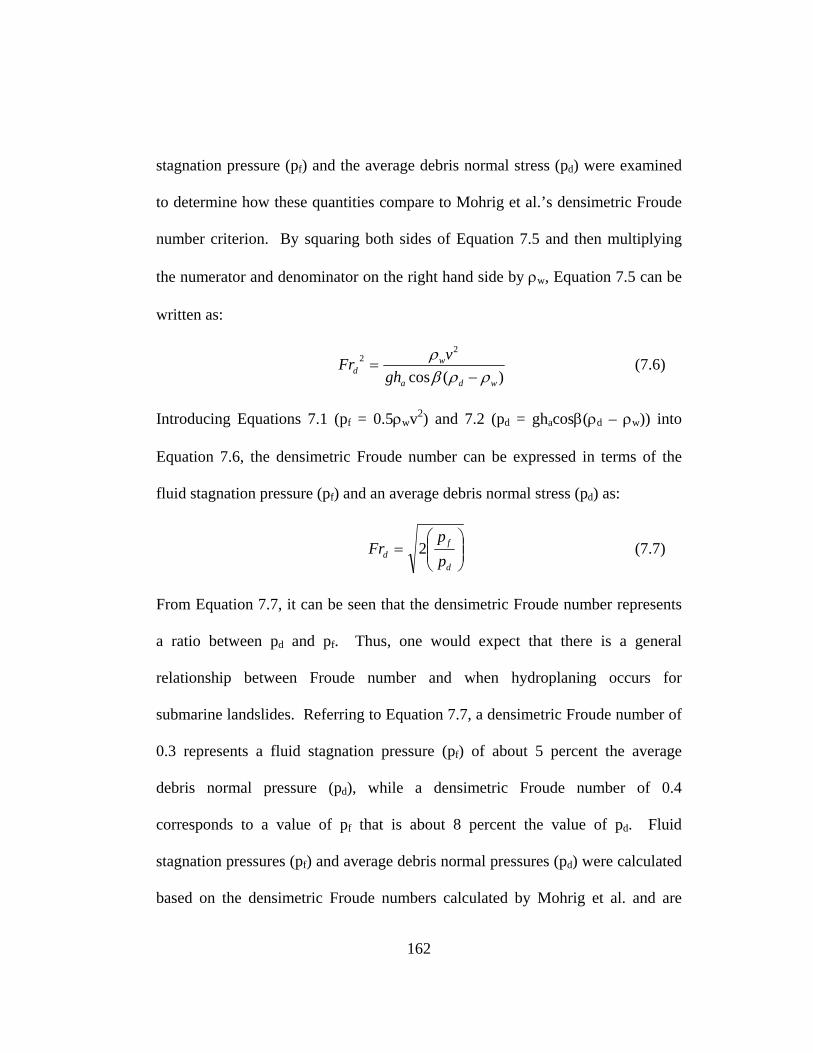
stagnation pressure (pf) and the average debris normal stress (pd) were examined
to determine how these quantities compare to Mohrig et al.’s densimetric Froude
number criterion. By squaring both sides of Equation 7.5 and then multiplying
the numerator and denominator on the right hand side by ρw, Equation 7.5 can be
written as:
)(cos
22
wda
wd gh
vFrρρβ
ρ−
= (7.6)
Introducing Equations 7.1 (pf = 0.5ρwv2) and 7.2 (pd = ghacosβ(ρd – ρw)) into
Equation 7.6, the densimetric Froude number can be expressed in terms of the
fluid stagnation pressure (pf) and an average debris normal stress (pd) as:
⎟⎟⎠
⎞⎜⎜⎝
⎛=
d
fd p
pFr 2 (7.7)
From Equation 7.7, it can be seen that the densimetric Froude number represents
a ratio between pd and pf. Thus, one would expect that there is a general
relationship between Froude number and when hydroplaning occurs for
submarine landslides. Referring to Equation 7.7, a densimetric Froude number of
0.3 represents a fluid stagnation pressure (pf) of about 5 percent the average
debris normal pressure (pd), while a densimetric Froude number of 0.4
corresponds to a value of pf that is about 8 percent the value of pd. Fluid
stagnation pressures (pf) and average debris normal pressures (pd) were calculated
based on the densimetric Froude numbers calculated by Mohrig et al. and are
162
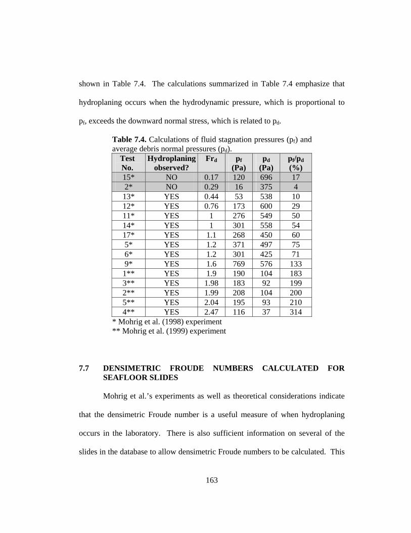
shown in Table 7.4. The calculations summarized in Table 7.4 emphasize that
hydroplaning occurs when the hydrodynamic pressure, which is proportional to
pf, exceeds the downward normal stress, which is related to pd.
Table 7.4. Calculations of fluid stagnation pressures (pf) and average debris normal pressures (pd).
Test No.
Hydroplaning observed?
Frd pf (Pa)
pd (Pa)
pf/pd (%)
15* NO 0.17 120 696 17 2* NO 0.29 16 375 4 13* YES 0.44 53 538 10 12* YES 0.76 173 600 29 11* YES 1 276 549 50 14* YES 1 301 558 54 17* YES 1.1 268 450 60 5* YES 1.2 371 497 75 6* YES 1.2 301 425 71 9* YES 1.6 769 576 133 1** YES 1.9 190 104 183 3** YES 1.98 183 92 199 2** YES 1.99 208 104 200 5** YES 2.04 195 93 210 4** YES 2.47 116 37 314
* Mohrig et al. (1998) experiment ** Mohrig et al. (1999) experiment
7.7 DENSIMETRIC FROUDE NUMBERS CALCULATED FOR SEAFLOOR SLIDES
Mohrig et al.’s experiments as well as theoretical considerations indicate
that the densimetric Froude number is a useful measure of when hydroplaning
occurs in the laboratory. There is also sufficient information on several of the
slides in the database to allow densimetric Froude numbers to be calculated. This
163

research effort involved examining the relationship between densimetric Froude
number and hydroplaning (slide runout distances) for several seafloor slides.
Sufficient data were available to permit densimetric Froude numbers to be
calculated for six of the slides in the database. Mohrig et al. (1998) calculated the
densimetric Froude number for five of the six slides. The calculated densimetric
Froude numbers and associated values of slope angle, thickness, and velocity
used for the calculations are summarized in Table 7.5. In all cases the velocities
that were reported for the case histories were based on observed damage to
submarine cables. For these case histories the cables were broken at known times
and locations, and velocities of the seafloor slides were then inferred. Also, slide
runout distances were not included in Mohrig et al. (1998), but were obtained
from the database. Runout distances are shown in Table 7.5 for comparison with
the calculated densimetric Froude numbers. The densimetric Froude numbers
range from 0.19 to 1.68. Based on Mohrig et al.’s (1998) criterion for
hydroplaning, that densimetric Froude numbers be at least 0.30 to 0.40,
hydroplaning should have occurred for five of the six landslides shown in Table
7.5. Also, the five slides where hydroplaning probably occurred had large runout
distances (> 20 km) and occurred on flat slopes as shown in Table 7.5. For the
one slide (Sandnessjoen slide) where the calculated Frd number (0.19) was less
than the threshold value required for hydroplaning, hydroplaning probably did not
occur due to the small runout distance and low Frd number. It can be seen in
164
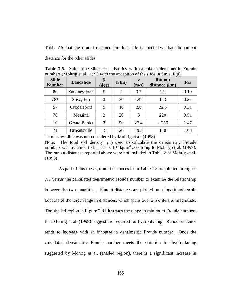
Table 7.5 that the runout distance for this slide is much less than the runout
distance for the other slides.
Table 7.5. Submarine slide case histories with calculated densimetric Froude numbers (Mohrig et al., 1998 with the exception of the slide in Suva, Fiji).
Slide Number Landslide β
(deg) h (m) v (m/s)
Runout distance (km) Frd
80 Sandnessjoen 5 2 0.7 1.2 0.19
78* Suva, Fiji 3 30 4.47 113 0.31
57 Orkdalsford 5 10 2.6 22.5 0.31
70 Messina 3 20 6 220 0.51
10 Grand Banks 3 50 27.4 > 750 1.47 71 Orleansville 15 20 19.5 110 1.68
* indicates slide was not considered by Mohrig et al. (1998). Note: The total soil density (ρd) used to calculate the densimetric Froude numbers was assumed to be 1.71 x 10³ kg/m3 according to Mohrig et al. (1998). The runout distances reported above were not included in Table 2 of Mohrig et al. (1998).
As part of this thesis, runout distances from Table 7.5 are plotted in Figure
7.8 versus the calculated densimetric Froude number to examine the relationship
between the two quantities. Runout distances are plotted on a logarithmic scale
because of the large range in distances, which spans over 2.5 orders of magnitude.
The shaded region in Figure 7.8 illustrates the range in minimum Froude numbers
that Mohrig et al. (1998) suggest are required for hydroplaning. Runout distance
tends to increase with an increase in densimetric Froude number. Once the
calculated densimetric Froude number meets the criterion for hydroplaning
suggested by Mohrig et al. (shaded region), there is a significant increase in
165

runout distance. Also, the runout distance can be highly variable, ranging almost
1.5 orders of magnitude.
1
10
100
1000
0.00 0.50 1.00 1.50 2.00
Densimetric Froude Number, Frd
Run
out D
ista
nce
(km
)
Hydroplaning
No Hydroplaning
Figure 7.8. Calculated densimetric Froude numbers versus runout distance based on six seafloor slides from the database. Shaded region indicates Froude number criterion (Frd of 0.30 to 0.40) for hydroplaning suggested by Mohrig et al. (1998). 7.8 SLIDES FROM THE DATABASE THAT MAY HAVE
HYDROPLANED Four of the five slides examined in the previous section are believed to
have hydroplaned based on the calculated densimetric Froude numbers and the
large runout distances (>20 km) that were achieved on flat slopes (< 5 deg). The
166
fifth slide (at Orleansville) occurred on a slope inclined at 15 degrees. The
characteristics of runout distance (>20 km) and slope angle (< 5 deg) for the four
slides were applied to the remainder of slides in the database that have
information available for runout distance and slope angle. Runout distance versus
slope angle was plotted in Figure 5.24 (Chapter 5) for 343 slides in the database.
This figure was plotted again to examine the slides in the database that the same
characteristics of slide runout as the slides that are believed to have hydroplaned,
i.e. runout distance > 20 km and β < 5 deg. This is shown in Figure 7.9 with a
shaded region indicating the criteria inferred for hydroplaning. There are about
60 slides that have data that plot in this shaded region. Based on the similar
runout characteristics as the four slides that are believed to have hydroplaned,
hydroplaning may have also occurred for these 60 slides.
167

0.1
1
10
100
1000
0 5 10 15 20 25 30
Slope Angle (deg)
Run
out D
ista
nce
(km
)
343 eventsHydroplaning may have occurred for slides in this region.
Figure 7.9. Slides that may have hydroplaned considering the characteristics of runout distance (> 20 km) and slope angle (< 5 deg). 7.9 ROLE OF SOIL STRENGTH IN PRODUCING REQUIRED
VELOCITIES FOR HYDROPLANING
For hydroplaning to occur, there must be sufficient velocity of the
landslide, and this is reflected in the requirement that the densimetric Froude
number be at least 0.30. As part of this thesis, the role of soil strength in
producing velocities required for hydroplaning was examined. The velocity of
the landslide sufficient for hydroplaning was expressed as:
168
⎟⎟⎠
⎞⎜⎜⎝
⎛−
=
1cos
30.0
w
da
CRIT
gh
v
ρρβ
(7.8)
The “critical slide velocity”, vCRIT, required to attain a densimetric Froude
number of at least 0.30 was computed from Equation 7.8 as follows:
⎟⎟⎠
⎞⎜⎜⎝
⎛−= 1cos*30.0
w
daCRIT ghv
ρρβ (7.9)
For this research effort, critical slide velocities, vCRIT, were calculated using the
data summarized for the five slides in Table 7.5, and are shown in Table 7.6 with
the inferred velocities that were based on known submarine cable breaks. All five
slides achieved velocities greater than the calculated “critical” slide velocity and,
thus, meet the velocity requirement for hydroplaning.
Table 7.6. Inferred velocities from submarine cable breaks and “critical” slide velocities for the five slides that hydroplaned.
Landslide Inferred velocity from case study
v (m/s)
“Critical” velocity
vCRIT (m/s) Grand Banks 27.4 5.6
Orkdalsfjord 2.6 2.5
Messina 6 3.5
Orleansville 19.5 3.5
Suva, Fiji 4.5 4.3
169
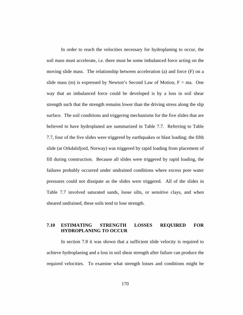
In order to reach the velocities necessary for hydroplaning to occur, the
soil mass must accelerate, i.e. there must be some imbalanced force acting on the
moving slide mass. The relationship between acceleration (a) and force (F) on a
slide mass (m) is expressed by Newton’s Second Law of Motion, F = ma. One
way that an imbalanced force could be developed is by a loss in soil shear
strength such that the strength remains lower than the driving stress along the slip
surface. The soil conditions and triggering mechanisms for the five slides that are
believed to have hydroplaned are summarized in Table 7.7. Referring to Table
7.7, four of the five slides were triggered by earthquakes or blast loading; the fifth
slide (at Orkdalsfjord, Norway) was triggered by rapid loading from placement of
fill during construction. Because all slides were triggered by rapid loading, the
failures probably occurred under undrained conditions where excess pore water
pressures could not dissipate as the slides were triggered. All of the slides in
Table 7.7 involved saturated sands, loose silts, or sensitive clays, and when
sheared undrained, these soils tend to lose strength.
7.10 ESTIMATING STRENGTH LOSSES REQUIRED FOR HYDROPLANING TO OCCUR
In section 7.8 it was shown that a sufficient slide velocity is required to
achieve hydroplaning and a loss in soil shear strength after failure can produce the
required velocities. To examine what strength losses and conditions might be
170
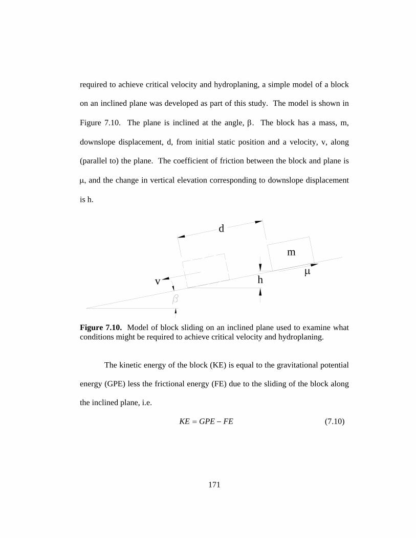
171
required to achieve critical velocity and hydroplaning, a simple model of a block
on an inclined plane was developed as part of this study. The model is shown in
Figure 7.10. The plane is inclined at the angle, β. The block has a mass, m,
downslope displacement, d, from initial static position and a velocity, v, along
(parallel to) the plane. The coefficient of friction between the block and plane is
µ, and the change in vertical elevation corresponding to downslope displacement
is h.
The kinetic energy of the block (KE) is equal to the gravitational potential
energy (GPE) less the frictional energy (FE) due to the sliding of the block along
the inclined plane, i.e.
hv
d
µ
m
Figure 7.10. Model of block sliding on an inclined plane used to examine what conditions might be required to achieve critical velocity and hydroplaning.
FEGPEKE −= (7.10)

172
Table 7.7. Soil conditions and triggering mechanisms of five seafloor slides believed to have hydroplaned.* Slide No.
Event Location
Soil Type Soil Properties Triggering Mechanism
10 Grand Banks Low plasticity clayey-silty fine sands along upper slope from around 500 mbsl; Low to medium plasticity clays along slope around 1000 – 1500 mbsl
Sensitive, strain-softening clays where w > LL (i.e. LI > 1.0, ~ 1.5); high sensitivity (S > 1.5); φ′ = 34o, c′ = 0 psf.
11/28/29 Earthquake (M = 7.2), slide occurred within epicentral region.
57 Orkdalsfjord,Norway
Failed material is very loose, soft non plastic silt
w ~ 33%; n ~ 49%, i.e. void ratio ~ 0.96
Man made slide (recent fill), Occurred on May 2, 1930
70 Messina, Italy Sand/Silt Earthquake loading (M = 7.5), occurred on 12/28/1908; slide occurred within epicentral region
71 El Asnam(formerly Orleansville)
Sand; well sorted (poorly graded), possibly alternating layers of sand and clay
Earthquake loading (M = 6.7), occurred on 9/9/1954; slide did not occur within epicentral region
78 Suva, Kadavupassage, Fiji
Sand Earthquake loading (M = 6.75), occurred in 1953; slide occurred within epicentral region
* Refer to database for references.

The gravitational potential energy (GPE) can be expressed as:
βsinmgdmghGPE == (7.11)
The frictional energy (FE) is expressed as:
βµ cosmgdFE = (7.12)
where µ is the coefficient of friction, or in terms of a friction angle, φ:
βφ costan mgdFE = (7.13)
Finally, the kinetic energy (KE) is expressed as:
25.0 mvKE = (7.14)
By combining Equations 7.10, 7.11, 7.13 and 7.14 and solving for velocity (v),
the velocity of the block is calculated as:
)cottan1(sin2 βφβ −= gdv (7.15)
The block begins to slide (incipient failure) when the friction angle
between the block and the inclined plane (φ) is equal to the angle of the plane (β),
i.e. tan φ cot β = 1 or φ = β. Suppose now, there is a loss in strength after
initiation of failure such that φ then becomes less than β. The loss in strength
after failure can be expressed as rφβ − where φr represents the reduced shear
strength after failure and the angle of the inclined plane remains constant.
Introducing the term rφβ − into Equation 7.15, the velocity of the block is then
calculated as:
173

( )φ
φβcos
)sin(2 rgdv −= (7.16)
Velocities were calculated from Equation 7.16 for various combinations of
downslope displacement, d, and strength losses, rφβ − . The friction angle at
failure, φ, is also a variable in Equation 7.16, and velocities were calculated
varying φ from 20 to 30 degrees, which were considered reasonable values.
Three scenarios of strength loss (1, 4, and 10 degrees) were considered in the
calculations, and are also believed to be reasonable values. One degree of
strength loss is a lower limit based on geotechnical testing capabilities, and ten
degrees of strength loss is considered an upper limit. Using four degrees of
strength loss, data for velocity as a function of downslope movement plot as an
“average” between the lower and upper limits. The velocity of the sliding block,
v, is plotted versus the downslope movement, d, for losses in strength of 1, 4, and
10 degrees as shown in Figure 7.10. Referring to Table 7.6, it can be seen that
“critical” slide velocities tend to be less than about 10 m/s (ranging from about 3
m/s to 6 m/s) based on the five case histories. This range in velocities (3 to 6 m/s)
is shown as a shaded region in Figure 7.11.
174
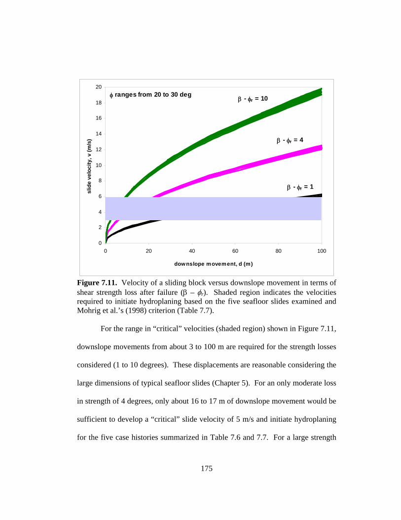
0
2
4
6
8
10
12
14
16
18
20
0 20 40 60 80 1
downslope movement, d (m)
slid
e ve
loci
ty, v
(m/s
)
00
β - φr = 4
β - φr = 1
φ ranges from 20 to 30 degβ - φr = 10
Figure 7.11. Velocity of a sliding block versus downslope movement in terms of shear strength loss after failure (β – φr). Shaded region indicates the velocities required to initiate hydroplaning based on the five seafloor slides examined and Mohrig et al.’s (1998) criterion (Table 7.7).
For the range in “critical” velocities (shaded region) shown in Figure 7.11,
downslope movements from about 3 to 100 m are required for the strength losses
considered (1 to 10 degrees). These displacements are reasonable considering the
large dimensions of typical seafloor slides (Chapter 5). For an only moderate loss
in strength of 4 degrees, only about 16 to 17 m of downslope movement would be
sufficient to develop a “critical” slide velocity of 5 m/s and initiate hydroplaning
for the five case histories summarized in Table 7.6 and 7.7. For a large strength
175
loss of 10 degrees only about 6 m of downslope movement would be sufficient to
initiate hydroplaning.
7.11 CONCLUSIONS
Hydroplaning of subaqueous slides occurs when a thin layer of fluid is
trapped between a sliding soil mass and the underlying soil. This mechanism may
account for large runout distances that have been observed for seafloor slides on
flat slopes. Hydroplaning occurs when the hydrodynamic pressure acting on the
front of the slide mass exceeds the normal stress exerted produced by the
submerged slide mass on the slip surface. The densimetric Froude number has
been shown to be a useful indicator of when hydroplaning occurs. From this
study, a slide velocity of about 3 to 6 m/s appears to be sufficient for
hydroplaning to occur based on five seafloor slides in the database and Mohrig et
al.’s (1998) criterion for hydroplaning (Frd ≥ 0.30). In order to achieve the
“critical” velocity required for hydroplaning, there must be a force imbalance
along the slip surface. This force imbalance could be provided by a loss in soil
shear strength. Characteristics of hydroplaning slides include:
1. deformation (distortion) of the front of slide mass (debris head) during
downslope movement
2. the thickness of the front of the slide mass (debris head) exceeding the
average thickness of the slide
176

3. in extreme cases, the frontal velocity exceeding the characteristic average
velocity, causing complete detachment and acceleration of the front of the
slide mass
4. the underlying soil remaining largely undisturbed by the overlying slide
mass
5. negligible influence of the rheological properties of the moving slide mass
(yield strength and viscosity) and channel bottom conditions (“soft”
versus “hard”)
The simple model of a sliding block developed for this thesis provides a
simple, effective way to evaluate the combinations of downslope movement,
strength loss, and slide velocity required to initiate hydroplaning. Based on this
model, movements of as little as 3 to 100 m accompanying a strength loss of 1 to
10 degrees could be enough to achieve “critical” velocity (3 to 6 m/s) and initiate
hydroplaning.
177
CHAPTER 8
RHEOLOGICAL MODELS
FOR SEAFLOOR SLIDE RUNOUT
8.1 INTRODUCTION
Several rheological models have been developed by others to address the
mechanics of submarine landslides during runout following the initial failure.
The rheological models treat the downslope movement of debris (soil) as a
flowing, fluid-like mass, rather than a sliding mass. Common rheological models
are described in this chapter. A one-dimensional, finite difference numerical
model that implements the rheological models in a computer program (BING) is
also described. The computer program was developed by Imran et al. (2001), and
was used by Imran et al. (2001) and Marr et al. (2002) to calculate runout
distances and thicknesses of submarine slides. The numerical simulations of
runout distance and slide thickness using the computer program have been
compared by Imran et al. (2001) to runout distances and slide thicknesses
observed for subaqueous slides in Mohrig et al.’s (1998, 1999) experiments
reported on in Chapter 7 and have been compared by Marr et al. (2002) to
seafloor slides in the Barents Sea.
178
8.2 RHEOLOGICAL MODELS
A description of rheology and various rheological models is presented in
this section. Three rheological models based on a viscoplastic material and a
“nonlinear” rheological model based on a combination of two classical types of
fluids are described.
8.2.1 OVERVIEW OF RHEOLOGY
Rheology is the study of the deformation and flow of matter. Rheological
models treat a moving slide mass as a flowing, fluid-like material; thus the soil
described in a rheological model is typically referred to as “fluid”, and fluid
mechanics principles are implemented. The amount of fines (minus No. 200
sieve), clay mineralogy, grain size distribution, and water content affect the
rheology of the “fluid”.
With rheological models, typical quantities used to define the properties of
materials are yield stress (strength), τy, and dynamic viscosity, η. These
quantities are defined by measurements of shear stress, τ, and rates of angular
deformation or shear strain, γ& or , using a viscometer. The yield stress, τdyud /& y,
is the shear stress required to cause motion of the “fluid”. Motion of the fluid
stops when the shear stress falls below the yield stress. The dynamic viscosity, η,
179

is the slope of the shear stress-shear strain rate curve, and depends on the type of
sediment and the rate of shear.
Classical types of fluids are “Newtonian”, “shear thickening”, “Bingham”,
and “Herschel-Bulkley”. The behavior of each of these types is illustrated in
Figure 8.1. Newtonian and Bingham fluids have a viscosity that remains constant
with shear strain rate. With shear thickening fluids, the viscosity increases with
increasing rate of shear strain, while Herschel-Bulkley fluids have a viscosity that
decreases with increasing rate of shear strain. Newtonian fluids have no yield
strength, τy, while shear thickening, Bingham, and Herschel-Bulkley fluids have a
yield strength. The viscosity and yield stress define how a viscous material
responds to forces such as friction, surface forces (frontal and drag), internal shear
and gravity.
180
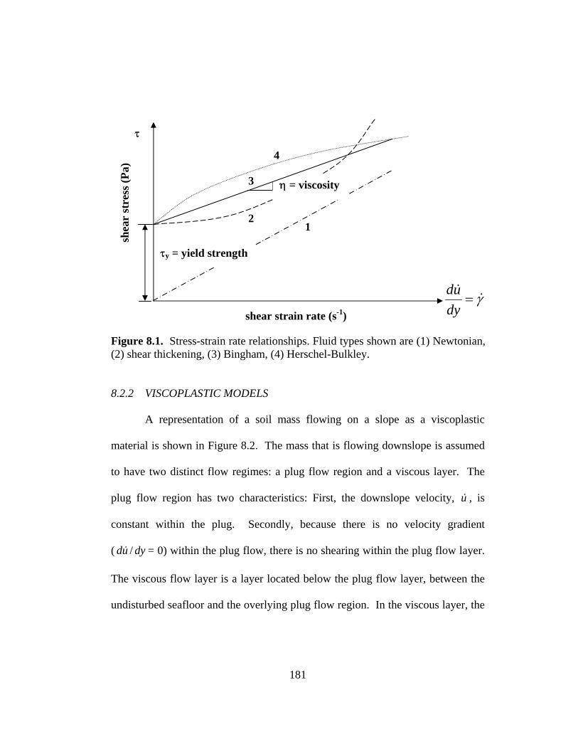
γ&&
=dyud
η = viscosity
τ
τy = yield strength
1
3
2
4
shea
r st
ress
(Pa)
shear strain rate (s-1)
Figure 8.1. Stress-strain rate relationships. Fluid types shown are (1) Newtonian, (2) shear thickening, (3) Bingham, (4) Herschel-Bulkley.
8.2.2 VISCOPLASTIC MODELS
A representation of a soil mass flowing on a slope as a viscoplastic
material is shown in Figure 8.2. The mass that is flowing downslope is assumed
to have two distinct flow regimes: a plug flow region and a viscous layer. The
plug flow region has two characteristics: First, the downslope velocity, u , is
constant within the plug. Secondly, because there is no velocity gradient
( = 0) within the plug flow, there is no shearing within the plug flow layer.
The viscous flow layer is a layer located below the plug flow layer, between the
undisturbed seafloor and the overlying plug flow region. In the viscous layer, the
&
dyud /&
181
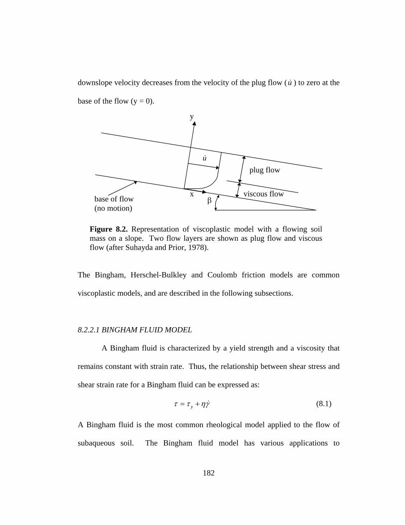
downslope velocity decreases from the velocity of the plug flow (u ) to zero at the
base of the flow (y = 0).
&
Figure 8.2. Representation of viscoplastic model with a flowing soil mass on a slope. Two flow layers are shown as plug flow and viscous flow (after Suhayda and Prior, 1978).
y
base of flow (no motion)
plug flow
viscous flow β
u&
x
The Bingham, Herschel-Bulkley and Coulomb friction models are common
viscoplastic models, and are described in the following subsections.
8.2.2.1 BINGHAM FLUID MODEL
A Bingham fluid is characterized by a yield strength and a viscosity that
remains constant with strain rate. Thus, the relationship between shear stress and
shear strain rate for a Bingham fluid can be expressed as:
γηττ &+= y (8.1)
A Bingham fluid is the most common rheological model applied to the flow of
subaqueous soil. The Bingham fluid model has various applications to
182

subaqueous soils. For example, Johnson (1970) studied the viscosity of silt and
sand particles in water and concluded that these particles behaved as a Bingham
fluid. Furthermore, Govier and Aziz (1982) found that high concentrations of
clay, silt, and sand in water behave as a Bingham fluid under low shear strain
rates.
8.2.2.2 HERSCHEL-BULKLEY FLUID MODEL
The Herschel-Bulkley fluid model is a modification of the Bingham model
where the fluid is characterized as “pseudo-plastic” material that “thins” with
increase in applied shear strain, i.e. “shear thinning”. Thus, the viscosity
decreases as the shear strain rate increases as shown in Figure 8.1. The shear
stress-shear strain rate relationship for a Herschel-Bulkley model is expressed by
an equation of the form:
ny γηττ &+= (8.2)
where n is less than one. This model is just the opposite of what one would
expect for soils. Typically the shear strength of soil increases with increasing rate
of shear strain, i.e. viscosity increases. So, most soils should be “shear
thickening”. However, O’Brien and Julien (1988) concluded that the Herschel-
Bulkley model defines the behavior of clay-water suspensions reasonable well at
high shear strain rates.
183
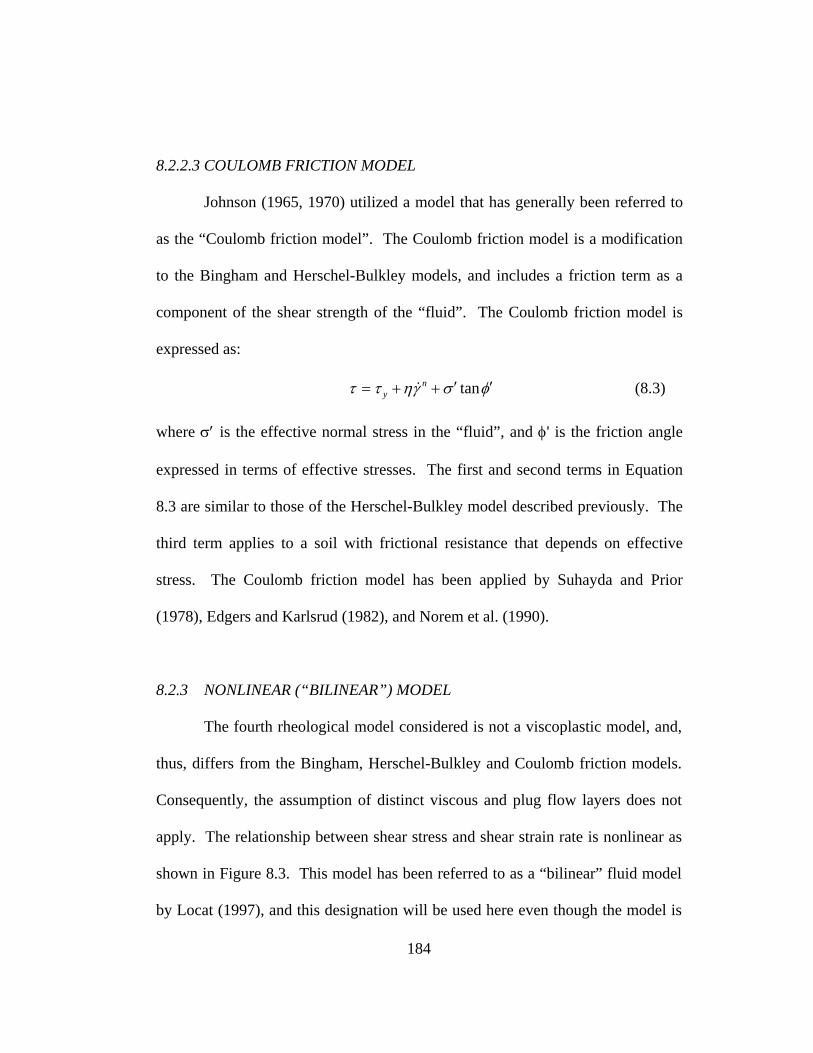
8.2.2.3 COULOMB FRICTION MODEL
Johnson (1965, 1970) utilized a model that has generally been referred to
as the “Coulomb friction model”. The Coulomb friction model is a modification
to the Bingham and Herschel-Bulkley models, and includes a friction term as a
component of the shear strength of the “fluid”. The Coulomb friction model is
expressed as:
φσγηττ ′′++= tanny & (8.3)
where σ′ is the effective normal stress in the “fluid”, and φ' is the friction angle
expressed in terms of effective stresses. The first and second terms in Equation
8.3 are similar to those of the Herschel-Bulkley model described previously. The
third term applies to a soil with frictional resistance that depends on effective
stress. The Coulomb friction model has been applied by Suhayda and Prior
(1978), Edgers and Karlsrud (1982), and Norem et al. (1990).
8.2.3 NONLINEAR (“BILINEAR”) MODEL
The fourth rheological model considered is not a viscoplastic model, and,
thus, differs from the Bingham, Herschel-Bulkley and Coulomb friction models.
Consequently, the assumption of distinct viscous and plug flow layers does not
apply. The relationship between shear stress and shear strain rate is nonlinear as
shown in Figure 8.3. This model has been referred to as a “bilinear” fluid model
by Locat (1997), and this designation will be used here even though the model is
184

actually nonlinear. The bilinear fluid is a hybrid of a Bingham and Newtonian
fluid. Qualitatively speaking, at sufficiently low strain rates, the fluid behaves as
a Newtonian fluid with a viscosity, η1, and no yield strength, τy. At sufficiently
high strain rates, the fluid behaves as a Bingham fluid with lower viscosity, η2.
γ&=dydu
Figure 8.3. Bilinear rheological model.
η2
η1
Bingham-type fluid
Newtonian-type fluid
τ
shea
r st
ress
(Pa)
shear strain rate (s-1)
The response of the bilinear fluid is expressed as:
⎟⎟⎠
⎞⎜⎜⎝
⎛+
++=0γγ
γηττ&&
&c
y (8.5)
where τy is the apparent yield strength, γ& 0 is a rheological constant with units of
the inverse of time, and c is an empirical constant that has a negative value and
units of pressure divided by time. Imran et al. (2001) calculated the stress-strain
rate response of a bilinear fluid like the one described by Equation 8.5. Selected
185
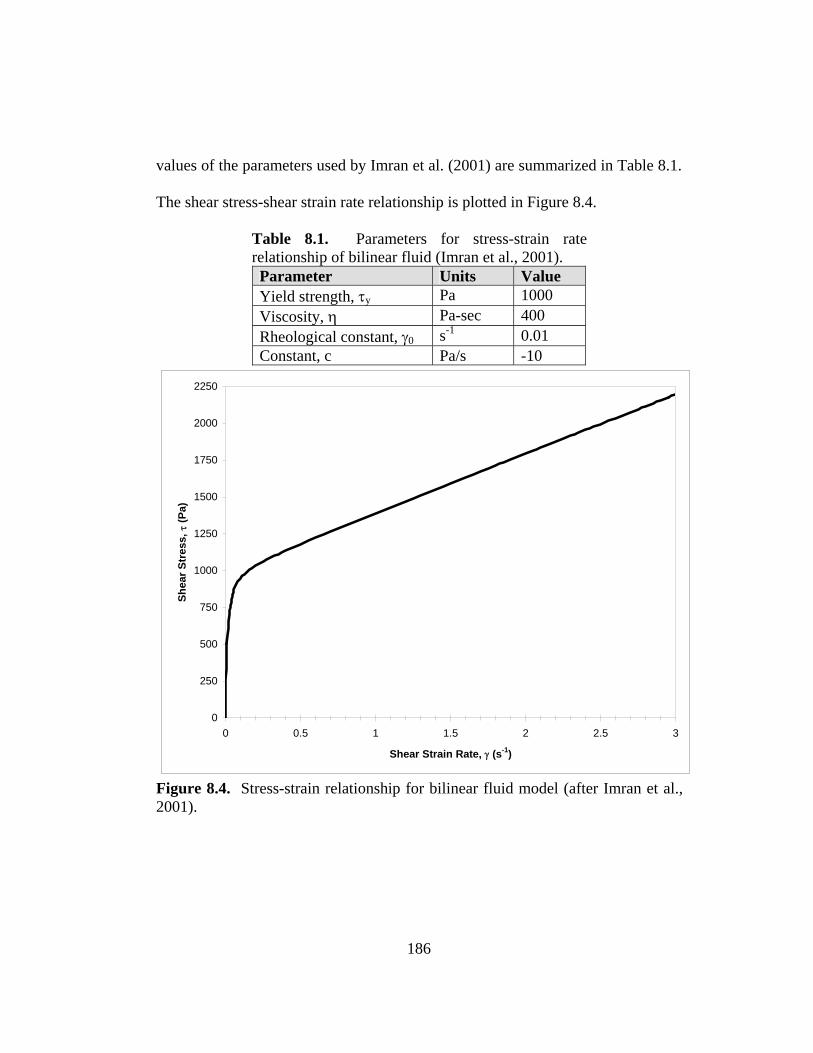
values of the parameters used by Imran et al. (2001) are summarized in Table 8.1.
The shear stress-shear strain rate relationship is plotted in Figure 8.4.
Table 8.1. Parameters for stress-strain rate relationship of bilinear fluid (Imran et al., 2001). Parameter Units Value Yield strength, τy Pa 1000 Viscosity, η Pa-sec 400 Rheological constant, γ0 s-1 0.01 Constant, c Pa/s -10
0
250
500
750
1000
1250
1500
1750
2000
2250
0 0.5 1 1.5 2 2.5
Shear Strain Rate, γ (s-1)
Shea
r Str
ess,
τ (P
a)
3
Figure 8.4. Stress-strain relationship for bilinear fluid model (after Imran et al., 2001).
186
8.3 NUMERICAL MODEL
A one-dimensional numerical model was developed by Imran et al. (2001)
to simulate debris flows based on Bingham, Herschel-Bulkley and bilinear fluid
models. The numerical model uses an explicit finite difference method to
conserve mass and momentum in debris flows assuming laminar flow. The
numerical model was implemented in a computer program called BING, and was
written in the Microsoft Visual Basic programming language. The computer
program has a graphical user interface. The program numerically simulates a
flowing mass and computes the runout distance, downslope velocity and
thickness of the deposit. Imran et al. (2001) studied the effect of the initial
geometry of the flow mass, the rheological model, and the rheological parameters
of viscosity and yield strength on the runout distance and thickness of the flow
mass. They also used their model to study the effect of the density of the material
that overlies the debris flow, i.e. air versus water, to examine possible differences
between subaerial and subaqueous debris flows.
A summary of input parameters for their simulations from the computer
program BING is shown in Table 8.2. The same values for the input parameters
were used for the analyses of subaerial and subaqueous flows, with the exception
of the mass density of the ambient material. For subaerial flows, the value for
ρAMBIENT (ρAIR) was 1 kg/m3, and for subaqueous flows, ρAMBIENT (ρWATER) was
187
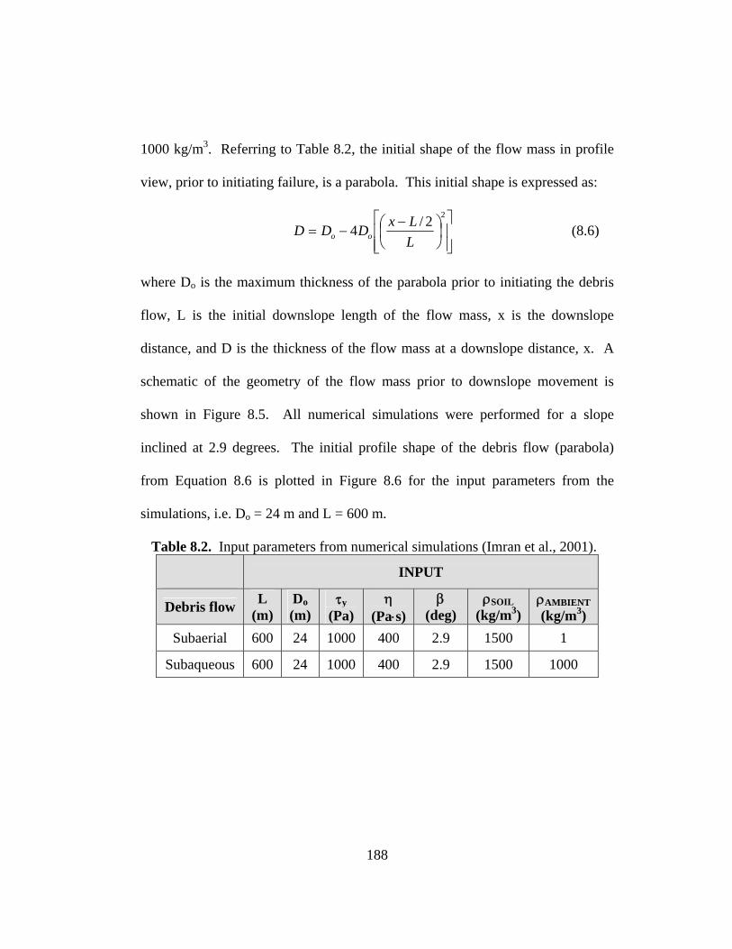
1000 kg/m3. Referring to Table 8.2, the initial shape of the flow mass in profile
view, prior to initiating failure, is a parabola. This initial shape is expressed as:
⎥⎥⎦
⎤
⎢⎢⎣
⎡⎟⎠⎞
⎜⎝⎛ −
−=22/4
LLxDDD oo (8.6)
where Do is the maximum thickness of the parabola prior to initiating the debris
flow, L is the initial downslope length of the flow mass, x is the downslope
distance, and D is the thickness of the flow mass at a downslope distance, x. A
schematic of the geometry of the flow mass prior to downslope movement is
shown in Figure 8.5. All numerical simulations were performed for a slope
inclined at 2.9 degrees. The initial profile shape of the debris flow (parabola)
from Equation 8.6 is plotted in Figure 8.6 for the input parameters from the
simulations, i.e. Do = 24 m and L = 600 m.
Table 8.2. Input parameters from numerical simulations (Imran et al., 2001). INPUT
Debris flow L (m)
Do (m)
τy (Pa)
η (Pa⋅s)
β (deg)
ρSOIL (kg/m3)
ρAMBIENT (kg/m3)
Subaerial 600 24 1000 400 2.9 1500 1
Subaqueous 600 24 1000 400 2.9 1500 1000
188
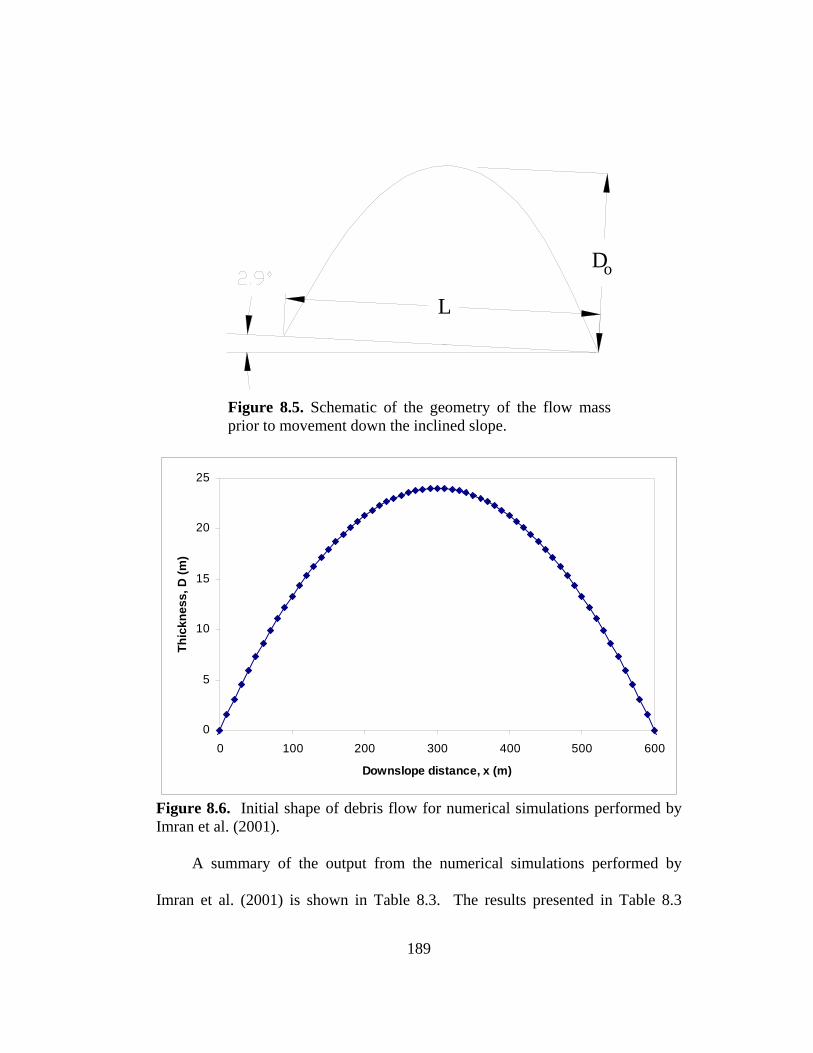
L
oD
Figure 8.5. Schematic of the geometry of the flow mass prior to movement down the inclined slope.
0
5
10
15
20
25
0 100 200 300 400 500 600
Downslope distance, x (m)
Thic
knes
s, D
(m)
Figure 8.6. Initial shape of debris flow for numerical simulations performed by Imran et al. (2001).
A summary of the output from the numerical simulations performed by
Imran et al. (2001) is shown in Table 8.3. The results presented in Table 8.3
189

show that the runout distance and peak velocity are greater for the subaerial
debris flow than for the subaqueous debris flow. The total time for runout, i.e.
from the time of initiation of downslope movement to the time the flow came to
rest, is also greater for the subaerial debris flow than for the subaqueous debris
flow.
Table 8.3. Output from the numerical simuations (Imran et al., 2001). OUTPUT
Debris flow Runout distance (m)
Peak velocity (m/s)
Total Time for Runout (min)
Subaerial 5,480 22.3 101.78
Subaqueous 1,571 9.86 21.95
The shapes of the debris flows from the simulations for the subaerial and
subaqueous flows are shown in Figure 8.7 in profile view. The thickness of the
debris flow is y, and is plotted normalized to the initial maximum thickness of the
flow (Do). The downslope length at time, t, is x, and is plotted normalized to the
initial length of the flow mass (L). The shapes of the debris flows at a downslope
travel (runout) time of 2 minutes are shown in Figure 8.7 (a), and the final shapes
of the debris flows at rest are shown in Figure 8.7 (b).
190
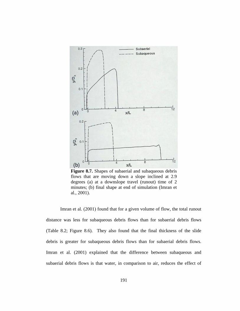
Figure 8.7. Shapes of subaerial and subaqueous debris flows that are moving down a slope inclined at 2.9 degrees (a) at a downslope travel (runout) time of 2 minutes; (b) final shape at end of simulation (Imran et al., 2001).
Imran et al. (2001) found that for a given volume of flow, the total runout
distance was less for subaqueous debris flows than for subaerial debris flows
(Table 8.2; Figure 8.6). They also found that the final thickness of the slide
debris is greater for subaqueous debris flows than for subaerial debris flows.
Imran et al. (2001) explained that the difference between subaqueous and
subaerial debris flows is that water, in comparison to air, reduces the effect of
191

gravity and impedes flow for subaqueous flows. However, Imran et al.’s findings
contradict most of the observations of Mohrig et al. (1998, 1999) who found that
when hydroplaning occurs, subaqueous debris flows can produce a thinner
deposit and travel longer distances than subaerial debris flows. In Chapter 7, it
was shown that 13 of the 15 subaqueous slides in Mohrig et al.’s (1998, 1999)
experiments were observed to hydroplane. Consequently, Imran et al. (2001)
found that simulations from their numerical model were only consistent with two
of the experimental observations of Mohrig et al. (1998). These were the two
tests where hydroplaning did not occur.
Marr et al. (2002) used Imran et al.’s (2001) computer program (BING) to
calculate runout distances and final thicknesses of slide deposits for seafloor
slides on the Isfjorden fan and the Bear Island fan in the Barents Sea. Data for
these seafloor slides were originally compiled by Laberg and Vorren (1993, 1995)
and Elverhøi et al. (1997). Marr et al. (2002) assumed that the soils behaved as a
Bingham fluid. A summary of the input parameters used for the numerical
simulations is shown in Table 8.4. Marr et al. (2002) state that the yield
strengths used in Cases 1 and 3 (Table 8.4) are representative of seafloor
sediments in the Barents Sea. On the other hand, Marr et al. (2002) state that
unreasonably low yield strengths, i.e. 1 to 5 kPa, were used as input for the
numerical simulation for Case 2 of the Bear Island debris flow.
192

Table 8.4. Input parameters for Marr et al.’s (2002) simulations.
Debris flow Initial shape
Slope Angle (deg)
L (km)
Do (m) τy (kPa) η
(Pa⋅s)
Isfjorden (Case 1) Parabola 3 – 4 6.67 90 10 - 25 300, 30
Bear Island (Case 2) Parabola 0.2 – 0.5 20 225 1 – 5 300, 30
Bear Island (Case 3) Parabola 0.2 – 0.5 20 225 10 - 25 300, 30
Output from Marr et al.’s (2002) numerical simulations is summarized in
Table 8.5. The observed runout distances and mean slide thicknesses are also
shown in Table 8.5 for comparison with the computed values. Numerical
simulations for slides on the Isfjorden fan were in good agreement with field
observations (Case 1), as shown in Table 8.5. Simulations for the slides on the
Bear Island fan were not in good agreement with field observations (Case 3)
when reasonable values for the yield strength were used. Simulations from Case
2 were in good agreement with field observations; however Marr et al. (2002)
stated that the yield strengths that were used in these computations (Case 2) were
not representative of field conditions. To explain the discrepancies between the
simulations and the actual observed results, Marr et al. (2002) attributed the Bear
Island fan slides, which have long runout distances of 100 to 200 km on slope
angles less than one degree, to a flow mechanism other than the Bingham fluid
model, such as hydroplaning. Thus the Bingham model does not appear to be
valid for the slides that occurred on the Bear Island fan.
193

Table 8.5. Observed runout characteristics and output from Marr et al.’s (2002) simulations.
Runout distance (km) Mean thickness (m)
Debris flow Observed BING Observed BING
Isfjorden (Case 1) 10 - 30 13 – 44 10 – 30 10 – 22
Bear Island (Case 2) 100 – 200 77 – 355 10 – 50 8 – 30
Bear Island (Case 3) 100 - 200 7 - 35 10 - 50 50 - 130
8.4 CONCLUSIONS
Imran et al.’s (2001) and Marr et al.’s (2002) numerical simulations of
runout distance and thickness of debris flows using a Bingham rheological model
were in good agreement with only 3 of the 17 cases considered, i.e. 2 of the 15
cases from Mohrig et al.’s (1998, 1999) experiments and 1 of the 2 seafloor slides
identified by Laberg and Vorren (1993, 1995) and Elverhøi et al. (1997). In
general, the observed runout distances were larger and the observed slide
thicknesses were smaller than those predicted by the numerical simulations.
Imran et al. (2001) and Marr et al. (2002) attributed the discrepancies in runout
distance and thickness of the debris flows to some additional mechanism such as
hydroplaning.
194

CHAPTER 9
SUMMARY, CONCLUSIONS,
AND RECOMMENDATIONS
9.1 SUMMARY AND CONCLUSIONS
An extensive review of the literature on seafloor slope failures has been
conducted, and data on 534 seafloor slope failures have been compiled in a
database. The database includes the date of failure, geographic location, soil
types, soil properties, causes of slope failure (triggering mechanisms), distance of
slide runout, slide thickness, total area influenced by slide, volume of slide mass,
slope angle, and shallowest and deepest water depths affected. Fourteen different
triggering mechanisms (triggers) were identified and are included in the database.
The triggers have been described in Chapter 4, and relevant information
pertaining to the triggers and how the information is included in the database have
also been described. Although there is a large amount of information in the
database, significant geotechnical information was lacking for most of the slope
failures.
Characteristics of the seafloor slope failures (slides) have been evaluated
and are summarized in tables and figures in Chapter 5. The data show that
seafloor slides generally affect large areas and volumes of soil, and they tend to
be larger than subaerial landslides. Also, in comparison to subaerial landslides,
195
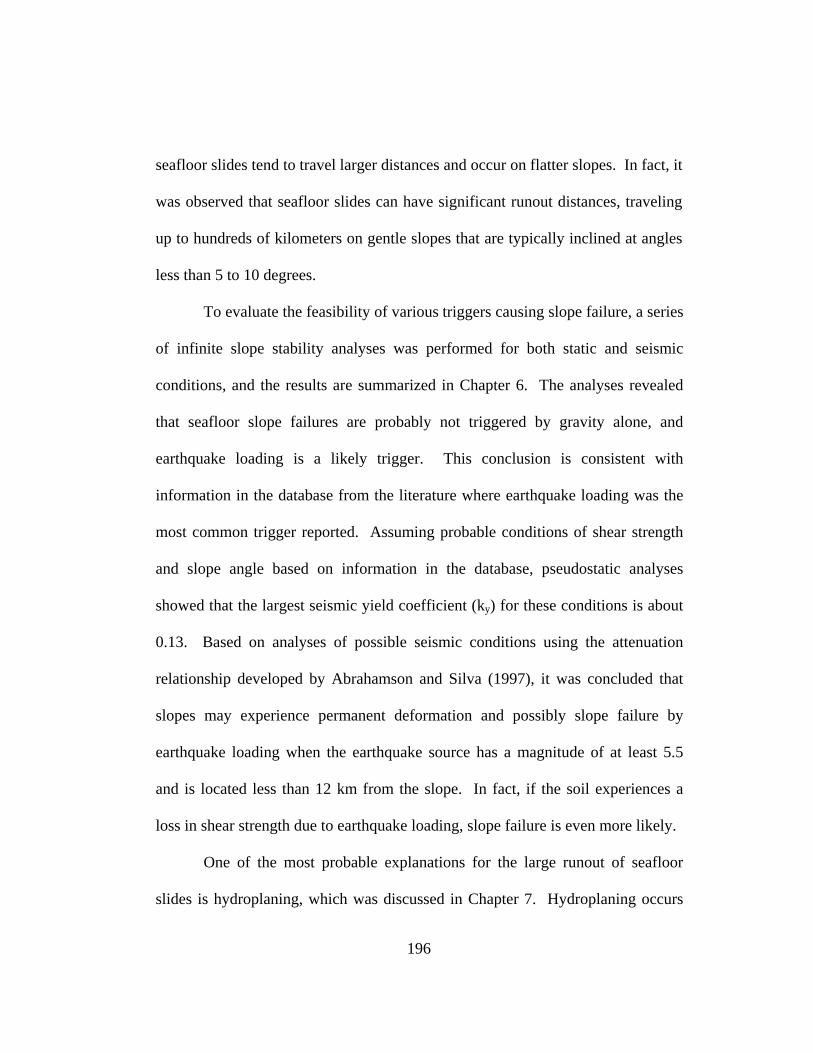
seafloor slides tend to travel larger distances and occur on flatter slopes. In fact, it
was observed that seafloor slides can have significant runout distances, traveling
up to hundreds of kilometers on gentle slopes that are typically inclined at angles
less than 5 to 10 degrees.
To evaluate the feasibility of various triggers causing slope failure, a series
of infinite slope stability analyses was performed for both static and seismic
conditions, and the results are summarized in Chapter 6. The analyses revealed
that seafloor slope failures are probably not triggered by gravity alone, and
earthquake loading is a likely trigger. This conclusion is consistent with
information in the database from the literature where earthquake loading was the
most common trigger reported. Assuming probable conditions of shear strength
and slope angle based on information in the database, pseudostatic analyses
showed that the largest seismic yield coefficient (ky) for these conditions is about
0.13. Based on analyses of possible seismic conditions using the attenuation
relationship developed by Abrahamson and Silva (1997), it was concluded that
slopes may experience permanent deformation and possibly slope failure by
earthquake loading when the earthquake source has a magnitude of at least 5.5
and is located less than 12 km from the slope. In fact, if the soil experiences a
loss in shear strength due to earthquake loading, slope failure is even more likely.
One of the most probable explanations for the large runout of seafloor
slides is hydroplaning, which was discussed in Chapter 7. Hydroplaning occurs
196
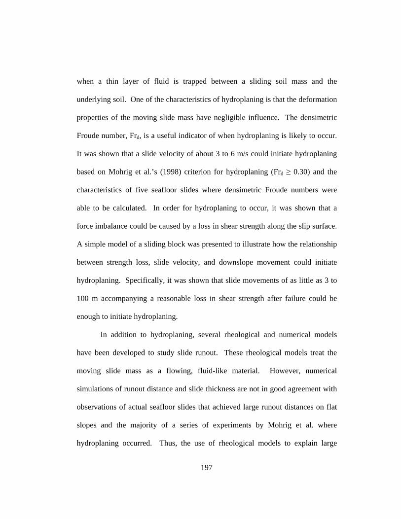
when a thin layer of fluid is trapped between a sliding soil mass and the
underlying soil. One of the characteristics of hydroplaning is that the deformation
properties of the moving slide mass have negligible influence. The densimetric
Froude number, Frd, is a useful indicator of when hydroplaning is likely to occur.
It was shown that a slide velocity of about 3 to 6 m/s could initiate hydroplaning
based on Mohrig et al.’s (1998) criterion for hydroplaning (Frd ≥ 0.30) and the
characteristics of five seafloor slides where densimetric Froude numbers were
able to be calculated. In order for hydroplaning to occur, it was shown that a
force imbalance could be caused by a loss in shear strength along the slip surface.
A simple model of a sliding block was presented to illustrate how the relationship
between strength loss, slide velocity, and downslope movement could initiate
hydroplaning. Specifically, it was shown that slide movements of as little as 3 to
100 m accompanying a reasonable loss in shear strength after failure could be
enough to initiate hydroplaning.
In addition to hydroplaning, several rheological and numerical models
have been developed to study slide runout. These rheological models treat the
moving slide mass as a flowing, fluid-like material. However, numerical
simulations of runout distance and slide thickness are not in good agreement with
observations of actual seafloor slides that achieved large runout distances on flat
slopes and the majority of a series of experiments by Mohrig et al. where
hydroplaning occurred. Thus, the use of rheological models to explain large
197
seafloor slide movements is probably not valid in many instances. Hydroplaning,
which Mohrig et al. (1999) suggest is independent of rheology, is the most likely
mechanism to account for the large runout distances observed for some seafloor
slides.
9.2 RECOMMENDATIONS FOR FUTURE WORK
Recommendations are provided in this section to refine the database that
was created as part of this thesis, to develop models that account for
hydroplaning, to develop a methodology for risk assessment, and to continue
experimental studies of hydroplaning.
9.2.1 THE DATABASE
The database is currently in the form of one, large table in Microsoft
Access®. It is recommended that this database be refined into smaller tables, e.g.
by the addition of tables for shear strengths and plasticity indices. Additional
information should also be obtained from existing literature and incorporated into
the database. This includes determining the area of seafloor surveyed in the
geophysical investigation for each case study and the reasons the investigations
occurred, i.e. who funded the investigation. A new field containing an overall
“data quality” factor that is a function of the certainty of the cause(s) of slope
failure and the geophysical information is also recommended. It is recommended
198
that further statistical analyses of data in the database be performed to determine
correlations among the triggering mechanisms, site conditions and subsequent
extent of seafloor slide movement.
9.2.2 MODELS
It is recommended that numerical, theoretical and analytical models be
developed that account for the hydroplaning mechanism that has been observed in
the laboratory by Mohrig et al. (1998, 1999) and has been inferred to occur in
some seafloor slides from the database. Important properties and parameters
required for the models, e.g. slide velocity, soil shear strength (and potential for
strength loss), and type of loading, should be identified. These models should be
calibrated so that results of runout distance and slide thickness are in agreement
with observations of actual seafloor slides.
9.2.3 RISK ASSESSMENT
Because seafloor slope failures can impact oil and gas production in
deepwater, the formulation and testing of a methodology for risk assessment of
seafloor slope instability is important and recommended. Selected offshore sites
should be used to demonstrate how a risk assessment can be applied, to show how
existing data on submarine slope failures may be used, and to determine the value
of obtaining additional site-specific information. The risk assessment should
199
begin with a decision tree framework that outlines the potential triggering
mechanisms for the site, the history of seafloor slope instability in the vicinity of
the site, and various consequences of slope failure. For example, the decision of
where to construct an oil pipeline is a practical example that might be used to
establish the decision tree. The decision could be to position the pipeline through
a region susceptible to slope failure (low cost of construction, yet large risk of
damage to pipe) or to re-route the pipeline through a region where there is little
indication of future slope instability (high cost of construction, yet small risk of
damage to pipe). As part of this decision tree framework, the value of obtaining
additional site-specific information to reduce the risk should then be determined.
9.2.4 EXPERIMENTAL STUDIES
Several further experimental studies are needed to understand
hydroplaning better. Following the work of Mohrig et al. (1998, 1999),
improvements and additional tests could include:
(1) developing an experimental facility with a length of at least 20 m and
slopes of less than 5 degrees; Mohrig et al.’s facility was only 10 m long,
and slope angles for the channel were 4.9, 6.0, 15.5, 16.0 and 20.0
degrees. Mohrig et al. (1998) performed one test on a 1-degree slope,
which represents actual seafloor conditions better, yet hydroplaning did
not occur.
200

(2) performing more tests where the bottom of the channel is an existing soil
deposit (“soft” bottom) to simulate actual seafloor conditions prior to
filling with water and introducing a subaqueous slide; Mohrig et al.
(1999) only performed 2 tests with a “soft” bottom.
(3) performing additional tests to better delineate when hydroplaning occurs
and when it does not and to define better the densimetric Froude number
required for hydroplaning to occur. Mohrig et al.’s (1998) criterion based
on the densimetric Froude number was developed based on results from
only eight tests where hydroplaning occurred and two tests where
hydroplaning did not occur.
201
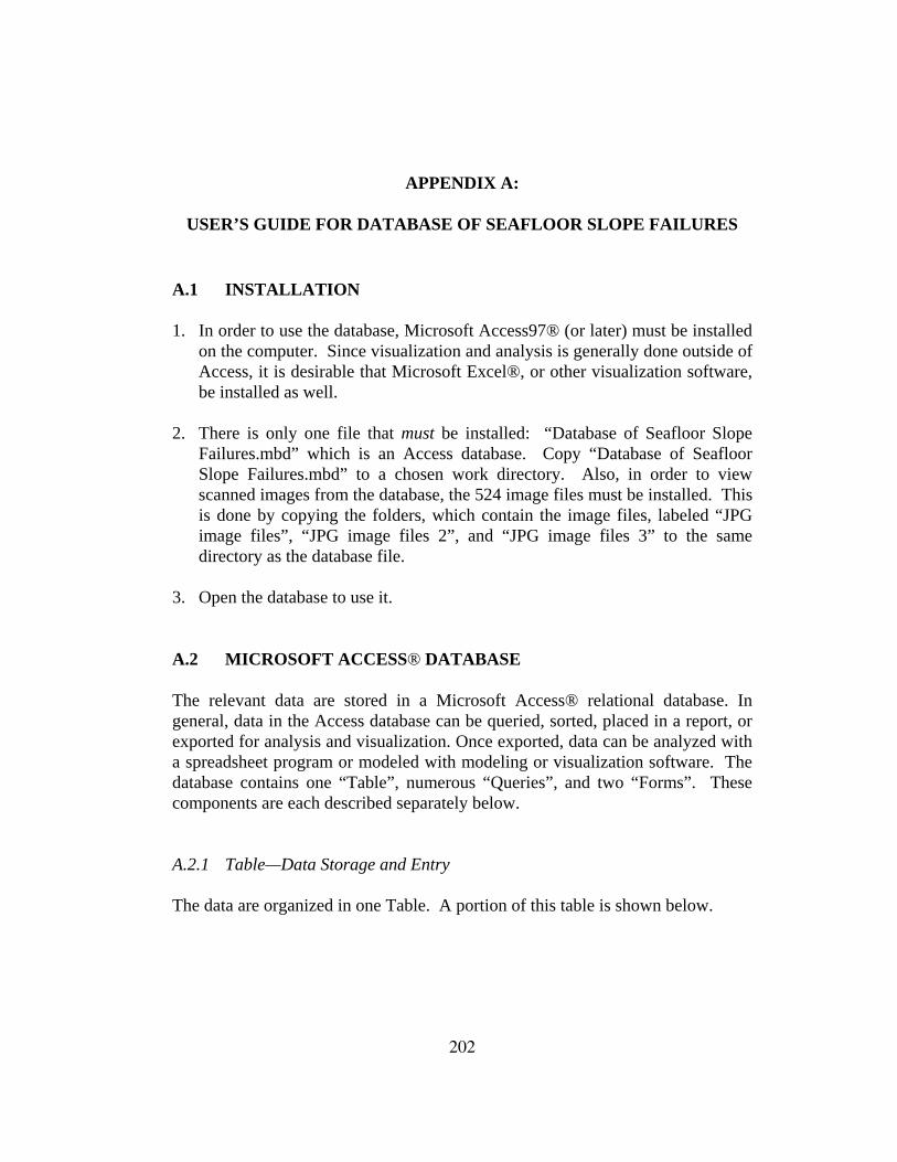
APPENDIX A:
USER’S GUIDE FOR DATABASE OF SEAFLOOR SLOPE FAILURES
A.1 INSTALLATION 1. In order to use the database, Microsoft Access97® (or later) must be installed
on the computer. Since visualization and analysis is generally done outside of Access, it is desirable that Microsoft Excel®, or other visualization software, be installed as well.
2. There is only one file that must be installed: “Database of Seafloor Slope
Failures.mbd” which is an Access database. Copy “Database of Seafloor Slope Failures.mbd” to a chosen work directory. Also, in order to view scanned images from the database, the 524 image files must be installed. This is done by copying the folders, which contain the image files, labeled “JPG image files”, “JPG image files 2”, and “JPG image files 3” to the same directory as the database file.
3. Open the database to use it. A.2 MICROSOFT ACCESS® DATABASE The relevant data are stored in a Microsoft Access® relational database. In general, data in the Access database can be queried, sorted, placed in a report, or exported for analysis and visualization. Once exported, data can be analyzed with a spreadsheet program or modeled with modeling or visualization software. The database contains one “Table”, numerous “Queries”, and two “Forms”. These components are each described separately below. A.2.1 Table—Data Storage and Entry The data are organized in one Table. A portion of this table is shown below.
202
Figure A.1. View of a portion of database Table. Data can be entered directly into the Table, and data can be extracted from the Table to create smaller tables. Data can also be modified and deleted. To modify data, highlight the incorrect entry and type a new one in its place. Records can be deleted by highlighting the entire record(s), and then Access will prompt you “do you really want to delete” the selected text. Data can also be entered into the Table from a spreadsheet by cutting and pasting. Entering data from a spreadsheet involves highlighting the data in the spreadsheet, copying it (to the clipboard), selecting the last record in the Access Table, and choosing “Paste Append” from the “Edit” menu. In pasting operations, it is necessary that the fields (columns) line up properly such that the widths of the columns are the same. A.2.2 Queries—Data Manipulation Queries are used to refine data from a dataset or to select certain types of information according to a specified criteria. There are two views for a Query:
203

“design” view and “table” view. An example Query for obtaining all case histories that have information available for slope angle and runout distance is shown below as it appears in the “design” view.
Figure A.2. “Design” view of query to extract all records with information available for average slope angle at failure and runout distance. Queries can retrieve information either from Tables or other Queries, and data can be modified through Queries. For example, if an error is detected during a Query it can be corrected in the Query and the corrections will be reflected in the Table and other Queries that contain that data. Design of a Query is generally a point and click operation with logical operators used to narrow down a selection. Access provides an “expression builder” when the user right clicks in the “criteria” field of the Query “design” view. For non-routine Queries, the on-line help is useful. Each field in the database has a specific type. The types of fields in the database are “number”, “text”, and “hyperlinks”, and there are several queries that were implemented for this database. For example, each “number” field was queried with a “>0” criterion to determine what slope failures have information in the specified field. Also, each “text” and “hyperlink” field was queried with a “* *” criterion. A space is always placed between the asterisks, which signifies there is data in that particular field. Another query method used for “text” and “hyperlink” fields is the “Is Null” criterion, which signifies there is no data in that particular field. If records are returned for the “Is Null” criterion, then these records do not have information for that particular field. The results from these search criteria (“>0”, “* *”, and “Is Null”) were noted and compared to the total number of slope failures in the database (534) in Table 5.1 in Chapter 5 of the thesis.
204
More than 50 Queries were created for the database. The queries that were used to extract information that was presented and summarized in this thesis are listed in Table A.1 along with a summary of the information that each query provides. The Queries for this database involve only the one Table that comprises the database. A.2.3 Forms—Automation Forms are used to make using the database more convenient. For example, forms may be used to automate common processes, or display data from a Table in a way more pleasing to the eye. A Form is based upon one or more Tables or Queries. The data in a Form may be displayed in datasheet mode (looks like a Table) or in standard form mode, which shows only one record at a time. You can toggle between the two modes by right-clicking the title bar of the Form and selecting the other view from the menu. Data may be entered or modified directly in a Form. While a Form is based on a Table or Query, the format of a Form is not automatically updated. For example, if you created a new field in a Table, that field would not automatically appear on an old Form. A standard form view for a landslide case history is shown below.
205
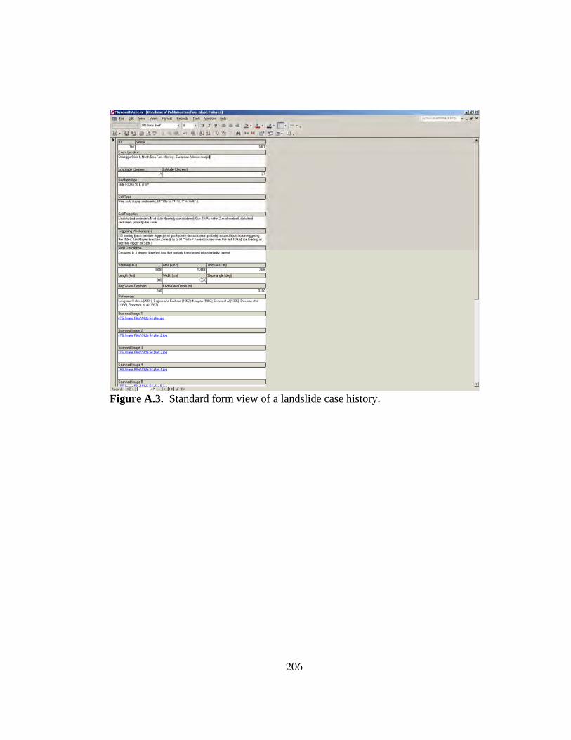
Figure A.3. Standard form view of a landslide case history.
206
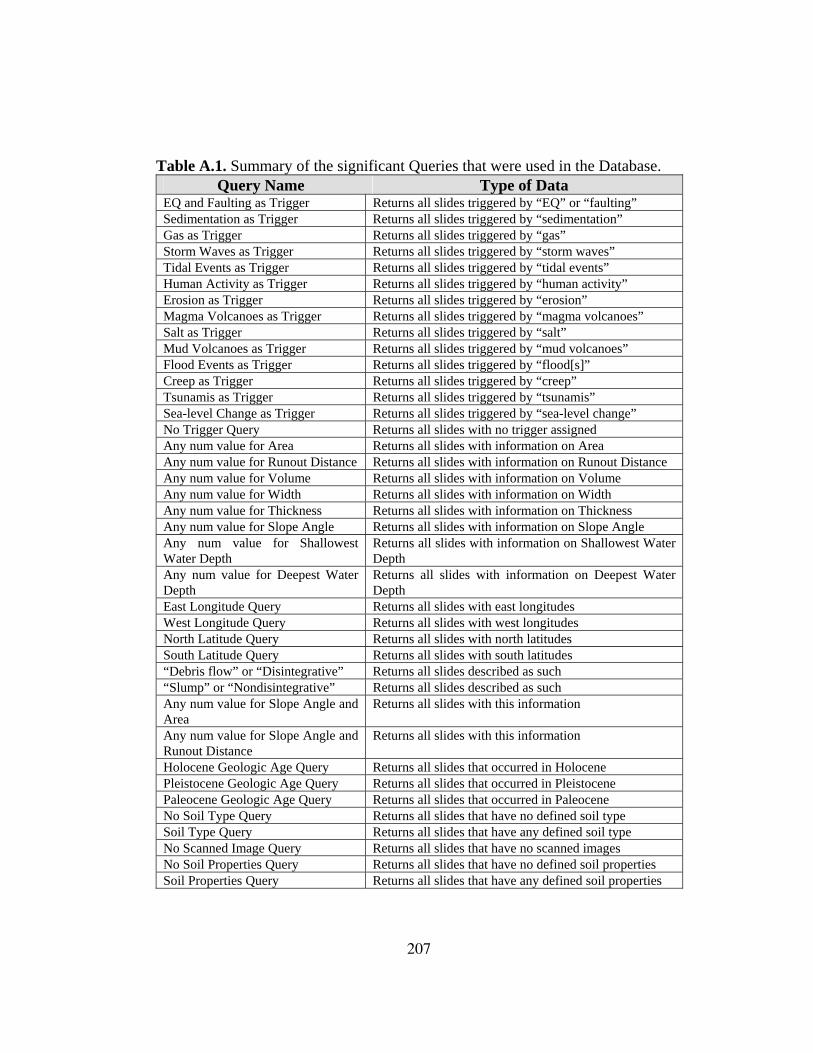
Table A.1. Summary of the significant Queries that were used in the Database. Query Name Type of Data
EQ and Faulting as Trigger Returns all slides triggered by “EQ” or “faulting” Sedimentation as Trigger Returns all slides triggered by “sedimentation” Gas as Trigger Returns all slides triggered by “gas” Storm Waves as Trigger Returns all slides triggered by “storm waves” Tidal Events as Trigger Returns all slides triggered by “tidal events” Human Activity as Trigger Returns all slides triggered by “human activity” Erosion as Trigger Returns all slides triggered by “erosion” Magma Volcanoes as Trigger Returns all slides triggered by “magma volcanoes” Salt as Trigger Returns all slides triggered by “salt” Mud Volcanoes as Trigger Returns all slides triggered by “mud volcanoes” Flood Events as Trigger Returns all slides triggered by “flood[s]” Creep as Trigger Returns all slides triggered by “creep” Tsunamis as Trigger Returns all slides triggered by “tsunamis” Sea-level Change as Trigger Returns all slides triggered by “sea-level change” No Trigger Query Returns all slides with no trigger assigned Any num value for Area Returns all slides with information on Area Any num value for Runout Distance Returns all slides with information on Runout Distance Any num value for Volume Returns all slides with information on Volume Any num value for Width Returns all slides with information on Width Any num value for Thickness Returns all slides with information on Thickness Any num value for Slope Angle Returns all slides with information on Slope Angle Any num value for Shallowest Water Depth
Returns all slides with information on Shallowest Water Depth
Any num value for Deepest Water Depth
Returns all slides with information on Deepest Water Depth
East Longitude Query Returns all slides with east longitudes West Longitude Query Returns all slides with west longitudes North Latitude Query Returns all slides with north latitudes South Latitude Query Returns all slides with south latitudes “Debris flow” or “Disintegrative” Returns all slides described as such “Slump” or “Nondisintegrative” Returns all slides described as such Any num value for Slope Angle and Area
Returns all slides with this information
Any num value for Slope Angle and Runout Distance
Returns all slides with this information
Holocene Geologic Age Query Returns all slides that occurred in Holocene Pleistocene Geologic Age Query Returns all slides that occurred in Pleistocene Paleocene Geologic Age Query Returns all slides that occurred in Paleocene No Soil Type Query Returns all slides that have no defined soil type Soil Type Query Returns all slides that have any defined soil type No Scanned Image Query Returns all slides that have no scanned images No Soil Properties Query Returns all slides that have no defined soil properties Soil Properties Query Returns all slides that have any defined soil properties
207
A.3 QUERY EXAMPLE To illustrate a typical Query, the following example is provided. The “design” view for this Query was shown previously in Figure A.2. This Query extracts all landslides that have information on slope angle and runout distance. In this example, the data are exported into an Excel® spreadsheet to be plotted. To create this Query, click the New button on the main Queries list. Select Design View and click OK. This brings up the Show Table window, which contains a list of available Tables and Queries that can be added to the Query. Select the Database of Seafloor Slope Failures Table by clicking Add since this is where the information of slope angle and runout distance is located. The fields of slope angle and runout distance are then queried by clicking-and-dragging from the Table in the upper half of the screen to a location in the lower half as shown in Figure A.4. Logical operators are then used to establish the criteria in the lower half. Criteria placed on the same row are “AND” criteria, while those on different rows are “OR” criteria. Criteria for this Query are placed in two fields. In this case, we want slides with any value for “Slope Angle (deg)” and “Runout Distance (km)”. In the row for criteria, type “>=0” for “Slope Angle (deg)” and for “Runout Distance (km)” on the same line (Figure A.4). This Query is then saved, named as Any num value for Slope Angle and Runout Distance, and viewed by clicking the Query View button on the upper left-hand corner of the screen. When the Query is complete, the output is then reviewed after clicking the Query View button. This output is shown in Figure A.5. The output is then exported into Excel. Since the cut and paste operation includes formats, it is often desirable to clear the formats after pasting into the spreadsheet (on the pull-down menu: Edit/Clear/ Formats). Figure A.6 shows the exporting command used from the “File” option on the toolbar.
208

Query view button
Upper half of screen
Lower half of screen
Figure A.4. Illustration of upper half and lower half of screen in Query “design” view.
209
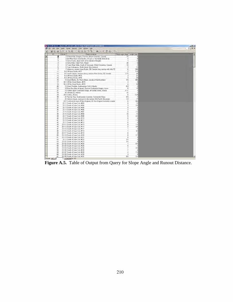
Figure A.5. Table of Output from Query for Slope Angle and Runout Distance.
210
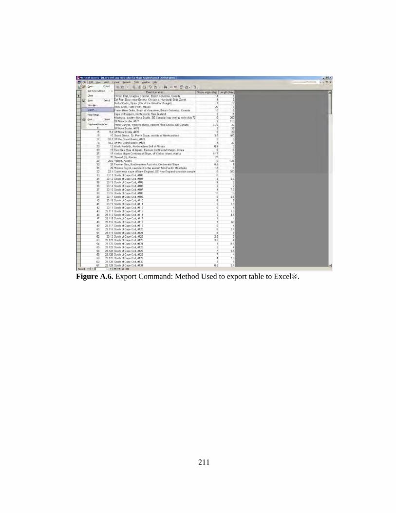
Figure A.6. Export Command: Method Used to export table to Excel®.
211
BIBLIOGRAPHY Abrahamson, N.A., and Silva, W.J., 1997. Empirical Response Spectral Attenuation Relations for Shallow Crustal Earthquakes. Seismological Research Letters, v. 68, no. 1. Almagor, G., 1978. Submarine slumping as a major agent of downslope sediment transport on the continental margin of Israel. International Congress on Sedimentology, 10th, v. 1, p. 15. * Almagor, G., 1980. Halokinetic deep-seated slumping on the Mediterranean slope of northern Sinai and southern Israel. Marine Geotechnology, v. 4, p. 83 – 105. * Almagor, G., and Wiseman, G., 1991. Analysis of submarine slumping in the continental slope off the southern coast of Israel. Marine Geotechnology, v. 10, p. 303-342. * Alonso, B., Kastens, K.A., Maldonado, A., Maliverno, A., Nelson, C.H., O’Connell, S., Palanques, A., and Ryand, W.B.F., 1985. Morphology of the Ebro fan valleys from SeaMARC and SeaBeam profiles, Geo-Marine Letters, v. 5, p. 141 – 148. Andersen, A., and Bjerrum, L., 1967. Slides in subaqueous slopes in loose sand and silt. Marine Geotechnique, p. 221 – 239. Andersen, E.S., Solheim, A., and Elverhoi, A., 1994. Development of a glaciated Arctic continental margin: Exemplified by the western margin of Svalbard. Proceedings, International Conference on Arctic Margins, 1992 (ICAM), p. 155 – 160. Assier-Rzadkieaicz, S., Heinrich, P., Sabatier, P.C., Savoye, B., Bourillet, J.F., 2000. Numerical Modelling of a Landslide-generated Tsunami: The 1979 Nice Event. Pure and Applied Geophysics, v. 157, issue 10, p. 1707-1727. * Bailey, E.B., Collet, L.W., and Field, R.M., 1928. Paleozoic submarine landslips near Quebec City. Journal of Geology, v. 36, p. 577 – 614. * Baltuk, M., Taylor, E. and McDougall, K., 1985. Mass movement along the inner wall of the Middle America Trench, Coast Rica, Initial Report of the Deep Sea Drilling Project, v. 84, p. 551 – 565. *
212

Baltzer, A., Cochonat, P., and Piper, D.J.W., 1994. In situ geotechnical characterization of sediments on the Scotian Slope, Eastern Canadian continental margin. Marine Geology, v. 120, p. 291-308. * Baltzer, A., Holmes, R. and Evans, D., 1998. Debris flows on the Sula Sgeir Fan, NW of Scotland. In Geological Processes on Continental Margins: Sedimentation, mass-wasting and stability, edited by M.S. Stoker, D. Evans, and A. Cramp, Geological Society, London, Special Publications, no. 129, p. 105-115. * Baraza, J., Ercilla, G., and Nilson, C.H., 1999. Potential geologic hazards on the eastern Gulf of Cadiz slope (SW Spain). Marine Geology, v. 155, p. 191 – 215. * Barnes, P.M., Cheung, K.C., Smits, A.P., Almagor, G., Read, S.A.L., Barker, P.R., and Froggatt, P., 1991. Geotechnical Analysis of the Kidnappers slide, upper continental slope, New Zealand. Marine Geotechnology, v. 10, p. 159-188. * Bartolini, C., Gehin, C., and Stanley, D.J., 1972. Morphology and recent sediments of the Alboran Basin in the Mediterranean Sea. Marine Geology, v. 13, p. 159-224. * Baumgartner, T., Ferreira, V., Soutar, Andrew, Schrader, H., and Moreno, F., 1985. Sedimentological implications of the reconstructed twentieth century varve record from the central Gulf of California. Eos, Transactions, American Geophysical Union, v. 66, no. 46, p. 917. * Bea, R.G., and Arnold, P., 1973. Movements and forces developed by wave-induced slides in soft clays, Offshore Technology Conference, Preprints, v. 2, p. 731 – 742. Bellaiche, G., Droz, L., Aloisi, J.-C., Bouye, C., Got, H., Monaco, A., Maldonado, A., Serra-Raventos, J., and Mirabile, L., 1981. The Ebro and the Rhone deep-sea fans: First comparative study. Marine Geology, v. 43, p. M75 – M85. * Bennett, R.H., Bryant, W.R., Dunlap, W.A., and Keller, G.H., 1976. Initial results and progress of the Mississippi Delta sediment pore water pressure experiment. Marine Geotechnology, v. 1, no. 4, p. 327 – 344.
213
Bennett, R.H., Lambert, D.N., and Hulbert, M.H., 1977. Geotechnical properties of a submarine slide area on the U.S. continental slope northeast of Wilmington Canyon. Marine Geotechnology, v. 2, p. 245-261. Bjerrum, L., 1971. Subaqueous slope failures in Norwegian fjords, International Conference on Port and Ocean Engineering under Arctic Conditions, Proceedings, v. 1, p. 24 – 47. * Bohlke, B.M., and Bennett, R.H., 1980. Mississippi prodelta crusts: a clay fabric and geotechnical analysis, Marine Geotechnology, v. 4, p. 55-82. Bondevik, S., Svendsen, J.I., Johnsen, G., Mangerud, J., and Kaland, P.E., 1997. The Storegga tsunami along the Norwegian coast, its age and runup. Boreas, v. 26, p. 29 – 53. * Booth, J.S., and O’Leary, D.W., 1991. A statistical overview of mass movement characteristics on the North America Atlantic Outer Continental Margin. Marine Geotechnology, v. 10, p. 1-18. * Booth, J.S., O’Leary, D.W., Popenoe, P., and Danforth, W.W., 1993. U.S. Atlantic Continental Slope Landslides: Their Distribution, General Attributes, and Implications. U.S. Geological Survey Bulletin 2002, Submarine Landslides: Selected Studies in the U.S. Exclusive Economic Zone, p. 14 – 22. * Bornhold, B.D., Ren, P., and Prior, D.B., 1994. High-frequency turbidity currents in British Columbia fjords. Geo-Marine Letters, v. 14, p. 238 – 243. * Bouma, A.H., Stelting, C.E., and Coleman, J.M., 1984. Mississippi Fan: Internal structure and depositional processes. Geo-Marine Letters, v. 3, p. 147 – 153. Buffler, R.T., Shaub, F.J., Watkins, J.S., and Worzel, J.L., 1979. Anatomy of the Mexican Ridges, Southwestern Gulf of Mexico. The American Association of Petroleum Geologists Special Publication, M 29: Geological and Geophysical Investigations of Continental Margins, p. 319 – 327. * Bugge, T., Befring, S., Belderson, R.H., Eidvin, T., Jansen, E., Kenyon, N.H., Holtedahl, H., and Sejrup, H.P., 1987. A giant three-stage submarine slide off Norway. Geo-Marine Letters, v. 7, p. 191 – 198. *
214
Bunn, A.R. and McGregor, B.A., 1980. Morphology of the North Carolina continental slope, Western north Atlantic, shaped by deltaic sedimentation and slumping, Marine Geology, v. 37, p. 253-266. * Butenko, J., and Barbot, J.P., 1979. Geological hazards related to offshore drilling and construction in the Orinoco river delta of Venezuela, Offshore Technology Conference, Proceedings, v. 1, p. 323 – 329. * Butler, L.W., 1979. Shallow structure on the continental margin, southern Brazil and Uruguay, Geological Society of America Bulletin, v. 81, p. 1079 – 1096. * Canals, A. M., and Chassefiere, B., 1989. Slump scars and eroded canyon walls on continental margins; implication for their geotechnical and mass physical properties; Gulf of Lions, Western Mediterranean Sea, Giornale di Geologia, v. 51, no. 1, p. 147 - 163. * Carlson, P.R., Karl, H.A., and Edwards, B.D., 1982. Puzzling mass movement features in the Navarinsky Canyon head, Bering Sea. Geo-Marine Letters, v. 2, p. 123 – 127. * Carlson, P.R., Karl, H.A., and Edwards, B.D., 1991. Mass sediment failure and transport features revealed by acoustic techniques, Beringian Margin, Bering Sea, Alaska. Marine Geotechnology, v. 10, p. 33-51. * Carlson, P.R., Karl, H.A., Edwards, B.D., Gardner, J.V., and Hall, R., 1993. Mass movement related to large submarine canyons along the Beringian Margin, Alaska. U.S. Geological Survey Bulletin 2002, Submarine Landslides: Selected Studies in the U.S. Exclusive Economic Zone, p. 104 - 116. * Carlson, P.R. and Molnia, B.F., 1977. Submarine Faults and slides on the continental shelf, northern Gulf of Alaska. Marine Geotechnology, v. 2, p. 275-290. * Carpenter, G.B., 1981a. Potential geologic hazards and constraints for blocks in proposed South Atlantic OCS Oil and Gas Lease Sale 56. U.S. Geological Survey Open-File Report 81-019, 286 p. Carpenter, G.B., 1981b. Coincident slump/clathrate complexes on the U.S. Atlantic continental slope, Geo-Marine Letters, v. 1, p. 29 - 32. *
215
Carpenter, G.B., Cardinell, A.P., Francois, D.K., Good, L.K., Lewis, R.L., and Stiles, N.T., 1982. Potential geologic hazards and constraints for blocks in proposed oil and gas lease sale 52. U.S. Geological Survey Open-File Report 82-36, 51 p. Carter, L., 2001. A large submarine debris flow in the path of the Pacific deep western boundary current off New Zealand. Geo-Marine Letters, v. 21, p. 42 – 50. * Carter, L., and Carter, R.M., 1985. Current modification of a mass failure deposit on the continental shelf, North Canterbury, New Zealand. Marine Geology, v. 62, p. 193 – 211. * Cashman, K.V. and Popenoe, P., 1985. Slumping and shallow faulting related to the presence of salt on the Continental Slope and Rise off North Carolina, Marine and Petroleum Geology, v. 2, p. 260 – 271. * Chamberlain, T.K., 1964. Mass transport of sediment in the heads of Scripps Submarine Canyon, California. In: Papers in marine geology; Shepard commemorative volume. Ed.: Miller, R.L., p. 42 – 64. * Chassefiere, B., and Monaco, A., 1989. Role of organic matter and particle fabric in mass-physical and geotechnical properties: Implications for undrained slumping in Aegean Sea and Ionian Sea modern sediments, Marine Geology, v. 87, p. 165 – 182. * Chen, M.-P., and Tian, W.-M., 1982. Marine geotechnical properties and stability of the continental margin deposits off Hua-Lien, northeast of Taiwan, Acta Oceanography Taiwanica, no. 13, p. 23 – 68. * Cherkis, N.Z., Max, M.D., Vogt, P.R., Crane, K., Midthassel, A., and Sundvor, E., 1999. Large-scale mass wasting on the north Spitsbergen continental margin, Arctic Ocean. Geo-Marine Letters, v. 19, p. 131 – 142. * Chough, S. K., Yoon, S. H., and Lee, H. J., 1992. Submarine slides in the eastern continental margin, Korea, Marine Geotechnology, v. 10, p. 71-82. * Chough, S. K., and Lee, H. J., 1987. Stability of sediments on the Ulleung Basin slope, Marine Geotechnology, v. 7, p. 123-132. *
216
Christian, H., Piper, D.J.W., and Armstrong, R., 1991. Geotechnical properties of seabed sediments from Flemish Pass. Deep Sea Research, v. 38, p. 663-676. Christian, H.A. et al, 1994. Slope instability on the Fraser River Delta Foreslope, Vancouver, British Columbia. Proceedings of the 47th CGS Conference in Halifax, p. 115-165. * Christian, H.A., Woeller, O.J., Robertson, P.K., and Courtney, R.C., 1997. Site investigations to evaluate flow liquefaction slides at Sand Heads, Fraser River delta, Canadian Geotechnical Journal, v 34, n 3, p. 384-397. * Cochonat, P., Bourillet, J.F., and Savoye, B., 1993. Geotechnical characteristics and instability of submarine slope sediments, the Nice slope (N-W Mediterranean Sea), Maine Georesources Geotechnology, v. 11, p. 131-151. * Cochonat, P., Ollier, G., and Michel, J.L., 1989. Evidence for slope instability and current-induced sediment transport, the RMS Titanic wreck search area, Newfoundland Rise, Geo-Marine Letters, v. 9, p. 145 – 152. * Coleman, J.M., and Garrison, L.E., 1978. Geological aspects of marine slope stability, northwestern Gulf of Mexico, Marine Geotechnology, v. 2, p. 9 - 44. * Corthay, J.E. II, and Aliyev, A.A., 2000. Delineation of a mud volcano complex, surficial mudflows, slump blocks, and shallow gas reservoirs, offshore Azerbaijan. Proceedings of the Annual Offshore Technology Conference, v. 1, 32nd Annual Offshore Technology Conference - OTC 2000, p. 327 – 354. * Coulter, H.W., and Migliaccio, R.R., 1966. Effects of the earthquake of March 27, 1964, at Valdez, Alaska. U.S. Geological Survey Professional Paper 542-C, 36 p. * Coumes, F., 1987. Seismic stratigraphy of giant mass movements, including megaturbidites, on recent continental margins. Geo-Marine Letters, v. 7, p. 113 – 117. * Damuth, J.E., and Flood, R.D., 1984. Morphology, sedimentation processes, and growth pattern of the Amazon deep-sea fan, Geo-Marine Letters, v. 3, p. 109 – 117. * Davis, S.N., and Karzulovic, K.J., 1963. Landslides at Lago Rinihue, Chile. Seismological Society of America Bulletin, v. 53, no. 6, p. 1403 – 1414. *
217
Davies, T.L., Van Niel, B., Kidd, R.B., and Weaver, P.P.E., 1997. High-resolution stratigraphy and turbidite processes in the Seine Abyssal Plain, northwest Africa. Geo-Marine Letters, v. 17, p. 147 – 153. * Daviess, S.N., 1971. Barbados: a major submarine gravity slide, Geological Society of America Bulletin, v. 82, p. 2593 – 2602. * Dawson, A.G., Long, D., and Smith, D.E., 1988. The Storegga slides: Evidence from eastern Scotland for a possible tsunami. Marine Geology, v. 82, p. 271 – 276. * Dengler, A.T., Wilde, P., Noda, E.K., and Normark, W.R., 1984. Turbidity currents generated by Hurricane Iwa. Geo-Marine Letters, v. 4, p. 5-11. * Desgagnes, P., Locat, J., Lee, H.J., Leroueil, S., Alexander, C., Mountain, G.,and Pratson, L., 2000. Geotechnical properties of a mass flow deposit on the Hudson Apron, off New Jersey, U.S.A., 53rd Canadian Geotechnical Conference, v. 1, p. 137 – 144. * Dillon, W.P., Popenoe, P., Grow, J.A., Klitgord, K.D., Swift, B.A., Paull, C.K., and Cashman, K.V., 1982. Growth faulting and salt diapirism—their relationship and control in the Carolina trough, eastern North America, in Watkins, J.S. and Drake, C.L. (eds.), Studies in continental margin geology. American Association of Petroleum Geologists Memoir 34, p. 31 – 46. Dillon, W.P., Risch, J.S., Scanlon, K.M., Valentine, P.C., and Huggett, Q.J., 1993. Ancient Crustal Fractures Control the Location and Size of Collapsed Blocks at the Blake Escarpment, East of Florida. U.S. Geological Survey Bulletin 2002, Submarine Landslides: Selected Studies in the U.S. Exclusive Economic Zone, p. 54 - 59. * Dimakis, P., Elverhøi, A., Hoeg, K., Solheim, A., Harbitz, C., Laberg, J.S., Vorren, T.O., and Marr, J., 2000. Submarine slope stability on high-latitude glaciated Svalbard-Barents Sea margin, Marine Geology, v. 162, p. 303-316. * Dingle, R. V., 1977. The anatomy of a large submarine slump on a sheared continental margin (SE Africa), Journal of the Geological Society of London, v. 134, Part 3, p. 293-310. *
218
Droz, L., Rigaut, F., Cochonat, P., and Tofani, R., 1996. Morphology and recent evolution of the Zaire turbidite system (Gulf of Guinea). Geological Society of America Bulletin, v. 108, p. 253-269. * Edgers, L., and Karlsrud, K., 1982. Soil flow generated by submarine slides – Case studies and consequences. In: C. Chryssostomidis and J.J. Connor (Eds.), Proceedings of the Third International Conference on the Behavior of Offshore Structures, Hemisphere, Bristol, Pa, p. 425-437. Edgers, L., and Karlsrud, K., 1985. Viscous analysis of submarine flows. Behaviour of Offshore Structures, p. 773 – 784. Edwards, B.D., Lee, H.J., and Field, M.E., 1993. Seismically Induced Mudflow in Santa Barbara Basin, California. U.S. Geological Survey Bulletin 2002, Submarine Landslides: Selected Studies in the U.S. Exclusive Economic Zone, p. 167-175. * Edwards, B.D., Field, M.E., and Clukey, E.C., 1980. Geological and geotechnical analysis of a submarine slump, California borderland, paper presented at 12th Annual Offshore Technology Conference, Proceedings, v. 1, p. 399-410. * Egloff, J., and Johnson, G.L., 1982. Growth fault on insular slope/rise of western Iceland; comparison with SE Greenland canyons and slumps. Geo-Marine Letters, v. 2, p. 143 – 148. * Elverhøi, A., Norem, H., Andersen, E.S., Dowdeswell, J.A., Fossen, I., Haflidason, H., Kenyon, N.H., Laberg, J.S., King, E.L., Sejrup, H.P., Solheim, A., and Vorren, T., 1997. On the origin and flow behavior of submarine slides on deep-sea fans along the Norwegian-Barents Sea continental margin. Geo-Marine Letters, v. 17, p. 119 – 125. * Embley, R.M., 1980. The role of mass transport in the distribution and character of deep-ocean sediments with special reference to the North Atlantic. Marine Geology, v. 38, p. 25-50. * Embley, R.M., 1976. New evidence for occurrence of debris flow deposits in the deep sea. Geology, v.4, n. 6, p. 371-374. * Embley, R.W., and Hayes, D.E., 1974. Giant submarine slump south of the Canaries, Geological Society of America, v. 6, p. 721. *
219
Embley, R.W. and Jacobi, R., 1977. Distribution and morphology of large submarine sediment slides and slumps on Atlantic continental margins. Marine Geotechnology, v. 2, p. 205-228. * Embley, R.W. and Morley, J., 1980. Quarternary sedimentation and paleoenvironmental studies off Namiba (southwest Africa). Marine Geology, v. 36, p. 183-204. * Emery, K.O., Uchupi, E., Phillips, J.D., Bowin, C.O., Bunce, E.T., and Knott, S.T., 1970. Continental rise off eastern North America. American Association of Petroleum Geologists Bulletin, v. 54, no. 1, p. 44 – 108. * Emery, K.O., Uchupi, E., Bowin, C.O., Phillips, J., and Simpson, E.S.W., 1975a. Continental margin off western Africa: Cape St. Francis (South Africa) to Walvis Ridge (South West Africa), American Association of Petroleum Geologists, Bulletin, v. 59, p. 3 - 59. * Emery, K.O., Uchupi, E., Phillips, J., Bowin, C.O., and Mascle, J., 1975b. Continental margin off Western Africa: Angola to Sierra Leone. American Association of Petroleum Geologists, Bulletin, v. 59, no. 12, p. 2209 – 2265. * Emmel, F.J., and Curray, J.R., 1984. The Bengal submarine fan, Northeastern Indian Ocean. Geo-Marine Letters, v. 3, p. 119 – 124. * Evans, D., King, E.L., Kenyon, N.H., Brett, C., and Wallis, D. 1996. Evidence for long-term instability in the Storegga Slide region off western Norway. Marine Geology, v. 130, p. 281-292. * Ferentinos, G., Brooks, M., and Collins, M., 1982. Gravity-induced deformation on the north flank and floor of the Sporadhes basin of the North Aegean sea trough, Marine Geology, v. 44, p. 289 – 302. Field, M.E., and Barber, J.H., 1993. A Submarine Landslide Associated with Shallow Sea-Floor Gas and Gas Hydrates off Northern California. U.S. Geological Survey Bulletin 2002, Submarine Landslides: Selected Studies in the U.S. Exclusive Economic Zone, p. 151-157. * Field, M.E., and Edwards, B.D., 1993. Submarine Landslides in a Basin and Ridge Setting, Southern California. U.S. Geological Survey Bulletin 2002, Submarine Landslides: Selected Studies in the U.S. Exclusive Economic Zone, p. 176 - 183. *
220

Field, M.E., and Edwards, B.D., 1980. Slopes of the southern California borderland: A regime of mass transport, in Field, M.E., Bouma, A.H., Colbourn, I.P., Douglas, R.G., and Ingle, J.C., eds., Pacific Section SEPM, Pacific Coast Paleogeography Symposium No. 4, Los Angeles, Calif., p. 169 – 184. * Field, M.E., and Gardner, J.V., 1990. Plio-Pleistocene growth of the Rio Ebro margin, NE Spain: A prograding slope model. Geological Society of America Bulletin, v. 102, p. 721 – 733. * Field, M.E., and Clarke, S.H., Jr., 1979. Small slumps and slides and their significance for basin slope processes, southern California borderland. Geology of continental slopes, Special Publication – Society of Economic Palentologists and Mineralogists, v. 27, p. 223 – 230. * Flaate, K., and Janbu, N., 1975. Soil exploration in a 500 m deep fjord, western Norway. Marine Geotechnology, v. 1, p. 117 – 139. Flood, R.D., Hollister, C.D. and Lonsdale, P., 1979. Disruption of the Fedi sediment drift by debris flows from Rockall Bank. Marine Geology, v. 32, p. 311-334. * Fortuin, A.R., Roep, Th.B., Sumosusatro, P.A., van Weering, Tj.C.E., and van der Werff, W., 1992. Slumping and sliding in Miocene and Recent developing arc basins, onshore and offshore Sumba (Indonesia), Marine Geology, v. 108, p. 345 – 363. * Fryer, G.J., 1996. Hawaiian tsunamis and small submarine landslides, AGU 1996 fall meeting, Eos, Transactions, American Geophysical Union, v. 77, no. 46, Suppl., p. 511. * Fryer, G.J., 1997. Landslides triggered by storm waves and tsunamis triggered by landslides: Unrecognized coastal hazards in Hawai’i, Abstracts with Programs - Geological Society of America, v. 29, no. 5, p. 14. Gardner, J.V., Prior, D.B., and Field, M.E., 1999. Humboldt Slide – a large shear-dominated retrogressive slope failure. Marine Geology, v. 154, p. 323 – 338. * Giardini, D., Grynthal, G., Shedlock, K., and Zhang, P., 1999. http://seismo.ethz.ch/GSHAP/.
221
Ginsburg, G.D., Kremlev, A.N., Grigor’vev, M.N., Pavlenkin, A.D., Larkin, G.V., and Tsar’kov, V.Ye., 1989. Discovery of solid gas hydrate in the rock at the foot of the continental slope of the Crimea. Transactions (Doklady) of the USSR Academy of Sciences: Earth Science Sections, v. 309, no. 6, p. 83 – 85. Goldfinger, C., Kulm, L.D., and McNeill, L.C., 1997. Super-scale slumping of the southern Oregon Cascadia margin; tsunamis and tectonic erosion of the forearc, Abstracts with Programs - Geological Society of America, v. 29, no. 5, p. 17. * Goldfinger, C., Kulm, L.D., McNeill, L.C., and Watts, P., 2000. Super-scale failure of the southern Oregon Cascadia margin. Pure and Applied Geophysics, v. 157, p. 1189-1226. * Gorsline, D.S., and Emery, K.O., 1959. Turbidity current deposits in San Pedro and Santa Monica Basins off southern California, Geological Society of America, Bulletin, v. 70, p. 279 – 290. * Grass, M., Watters, R., Karlin, R., and Holmes, M., 1997. Submarine and subaerial landslides as tools for paleoseismic analysis in the Puget Sound region, Washington State, Eos, Transactions, American Geophysical Union, v. 78, no. 46, Suppl., p. 440. * Grass, M., Watters, R., and Karlin, R., 1997. Paleoseismic analysis using submarine landslides in Puget Sound, Washington, Abstracts with Programs - Geological Society of America, v. 29, no. 5, p. 17. * Greene, H.G., Clarke, S.H., Field, M.E., Linker, F.I., and Wagner, H.C., 1975. Preliminary report on the environmental geology of selected areas of the Southern California Continental Borderland. U.S. Geological Survey Open-File Report 75-596. * Gutmacher, C.E., and Normark, W.R., 1993. Sur Submarine Landslide, a Deep-Water Sediment Slope Failure. U.S. Geological Survey Bulletin 2002, Submarine Landslides: Selected Studies in the U.S. Exclusive Economic Zone, p. 158-166. * Hampton, M.A., 1972. The role of subaqueous debris flow in generating turbidity currents. Journal of Sedimentary Petrology, v. 42, no. 4, p. 775 – 793. * Hampton, M.A., 1989. Geotechnical properties of unconsolidated sediment on the Kodiak continental shelf and upper slope, Gulf of Alaska. Marine Geotechnology, v.8, p. 159-180. *
222
Hampton, M.A., 1993. Comparison of Tectonic and Stratigraphic Control of Submarine Landslides on the Kodiak Upper Continental Slope, Alaska. U.S. Geological Survey Bulletin 2002, Submarine Landslides: Selected Studies in the U.S. Exclusive Economic Zone, p. 117-122. * Hampton, M.A., Lemke, R.W., and Coulter, H.W., 1993. Submarine Landslides that had a Significant Impact on Man and his Activities: Seward and Valdez, Alaska. U.S. Geological Survey Bulletin 2002, Submarine Landslides: Selected Studies in the U.S. Exclusive Economic Zone, p. 123-134. * Hampton, M.A., Lee, H.J., and Locat, J., 1996. Submarine Landslides. Reviews of Geophysics, v. 34, no. 1, p. 33-59. Hampton, M.A., and Bouma, A.H., 1977. Slope instability near the shelf break, western Gulf of Alaska. Marine Geotechnology, v.2, p. 309-331. * Hampton, M.A., Bouma, A.H., Carlson, P.R., Molnia, B.F., Clukey, E.C., 1978. Quantitative study of slope instability in the Gulf of Alaska, Offshore Technology Conference, 10. Houston 1978. Proceedings, v. 4, p. 2307 – 2318. * Hampton, M.A., and Winters, W.J., 1981. Environmental geology of Shelikof Strait, OCS Sale Area 60, Alaska, Offshore Technology Conference, 13. Houston 1981. Proceedings, p. 19 – 31. * Haner, B. E., and Gorsline, D. S., 1978. Processes and morphology of continental slope between Santa Monica and Dume submarine canyons, southern California, Marine Geology, v. 28, p. 77-87. * Heezen, B.C. and Ewing, M., 1952. Turbidity currents and submarine slumps, and the 1929 Grand Banks earthquake, American Journal of Science, v. 250, p. 849 – 873. * Heezen, B.C. and Ewing, M., 1955. Orleansville earthquake and turbidity currents, American Association of Petroleum Geologists Bulletin, v. 39, no. 12, p. 2505 – 2514. * Heezen, B.C. and Drake, C.L., 1964. Grand Banks slump. American Association of Petroleum Geologists Bulletin, v. 48, p. 221 – 233. *
223

Henkel, D.J., 1970. The role of waves in causing submarine landslides, Geotechnique, v. 20, p. 75 – 80. Herzer, R.H., 1979. Submarine landslides and submarine canyons on the slope off Canterbury, New Zealand, Journal of Geology and Geophysics, v. 22, no. 3, p. 391 – 406. * Herzer, R.H. and Lewis, D.W., 1979. Growth and burial of a submarine canyon off Motunau, North Canterbury, New Zealand, Sedimentary Geology, v. 24, no. 1, p. 69 – 83. * Hill, P.R., Moran, K.M., and Blasco, S.M., 1982. Creep deformation of slope sediments in the Canadian Beaufort Sea. Geo-Marine Letters, v. 2, p. 163 – 170. * Hill, P.R., 1983. Detailed morphology of a small area on the Nova Scotian Continental Slope. Marine Geology, v. 53, p. 55 – 76. * Hiscott, R.N., and Aksu, A.E., 1994. Submarine debris flows and continental slope evolution in front of Quaternary ice sheets, Baffin Bay, Canadian Arctic, American Association of Petroleum Geologists Bulletin, v. 78, no. 3, p. 445 – 460. * Holcomb, R., and Searle, R., 1991. Large landslides from oceanic volcanoes. Marine Geotechnology, v. 10, p. 19-32. * Holmes, R., Long, D., Dodd, L.R., 1998. Large-scale debrites and submarine landslides on the Barra Fan, west of Britain. In Geological Processes on Continental Margins: Sedimentation, mass-wasting and stability, edited by M.S. Stoker, D. Evans, and A. Cramp, Geological Society, London, Special Publications, no. 129, p. 67-79. * Holtedahl, H., 1965. Recent turbidites in the Hardangerfjord, Norway. Colston Research Society Proceedings, Bristol, v. 17, p. 107 – 141. * Hoskin, C.M., and Burrell, D.C., 1972. Sediment transport and accumulation in a fjord basin, Glacier Bay, Alaska. Journal of Geology, v. 80, p. 539 - 551. * Houtz, R.E., 1962. The 1953 Suva earthquake and tsunami. Bulletin of the Seismological Society of America, v. 52, p. 1-12. *
224

Houtz, R.E., and Wellman, H.W., 1962. Turbidity current at Kadavu passage, Fiji. Geological Magazine, v. 99, p. 57 – 62. * http://walrus.wr.usgs.gov/globalhydrate Huson, W.J. and Fortuin, A.R., 1985. The Lithinon Slide: A large submarine slide in the South Cretan Trough, eastern Mediterranean. Marine Geology, v. 65, p. 103 – 111. * Hwang, I.G., and Chough, S.K., 2000. The Maesan fan delta, Miocene Pohang Basin, SE Korea: architecture and depositional processes of a high-gradient fan-delta-fed slope system. Sedimentology, v. 47, p. 995 – 1010. * Hynes, M.E., and Franklin, A.G., 1984. Rationalizing the Seismic Coefficient Method. Miscellaneous Paper GL-84-13. US Army Engineer Waterways Experiment Station, Vicksburg, MS. Imamura, F., and Kikuchi, M., 1994. Moment release of the 1992 Flores Island earthquake inferred from tsunami and teleseismic data. Sci. Tsunami Hazards, v. 12, p. 67 – 76. * Imran, J., Parker, G., Locat, J., and Lee, H., 2001. 1D numerical model of muddy subaqeuous and subaerial debris flows, Journal of Hydraulic Engineering, v. 127, no. 11, p. 959 – 968. Jacobi, R. 1976. Sediment slides on the northwestern continental margin of Africa, Marine Geology, v. 22, p. 157-173. * Jacobi, R. and C.L. Mrozowski, 1979. Sediment slides and sediment waves in the Bonin Trough, western Pacific. Marine Geology, v. 29, no. ¼, p. M1 – M9. * Jenkins, C.J. and Keene, J.B., 1992. Submarine slope failures of the southeast Australian continental slope: a thinly sedimented margin. Deep-Sea Research, v. 39, no. 2, p. 121-136. * Johns, et al, 1986. Geotechnical aspects of a submarine slope failure, Kitimat Fjord, British Columbia. Marine Geotechnology, v. 6, no. 3, p. 243-279. * Jones, O.T., 1937. On sliding and slumping of submarine sediments in Denbighshire, North Wales during the Ludlow period. Geological Society of London Quarterly Journal, v. 93, p. 241 – 284. *
225
Josenhans, H.W., Barrie, J.V., and Kiely, L.A., 1987. Mass wasting along the Labrador shelf margin: Submersible observations. Geo-Marine Letters, v. 7, p. 199 – 205. * Karig, D.E., Barber, A.J., Charlton, T.R., Klemperer, S., and Hussong, D.M., 1987. Nature and distribution of deformation across the Banda Arc-Australian collision zone at Timor, Geological Society of America Bulletin, v. 98, p. 18 – 32. Karlin, R.E., Watters, R.J., Grass, M.J., Prunier, C.F., Holmes, M.L., 1996. Seismic landslides in Puget Sound (SLIPS); II, Quaternary faulting and submarine mass-wasting, AGU 1996 fall meeting, Eos, Transactions, American Geophysical Union, 77 (46, Suppl.), p. 499. Kayen, R.E., Schwab, W.C., Lee, H.J., Torresan, M.E., Hein, J.R., Quinterno, P.J., and Levin, L.A., 1989. Morphology of sea-floor landslides on Horizon Guyot: application of steady-state geotechnical analysis. Deep-Sea Research, v. 36, no. 12, p. 1817-1839. * Kayen, R.E., and Lee, H.J., 1991. Pleistocene slope instability of gas hydrate-laden sediment on the Beaufort Sea margin, Marine Geotechnology, 10 (1-2), p. 125-141. * Kayen, R. E., and Lee, H. J., 1993. Slope stability in regions of sea-floor gas hydrate; Beaufort Sea continental slope. U.S. Geological Survey Bulletin 2002, Submarine Landslides: Selected Studies in the U.S. Exclusive Economic Zone, p. 97-103. * Keating, B.H., Helsley, C.E., and Karogodina, I., 2000. Sonar studies of submarine mass wasting and volcanic structures off Savaii Island, Samoa. Pure and Applied Geophysics, v. 157, p. 1285 – 1313. * Keefer, D.K., 1984. Landslides caused by earthquakes. Geological Society of America Bulletin, v. 95, p. 406 – 421. * Keer, F.R. and Cardinell, A.P., 1981. Potential geologic hazards and constraints for blocks in proposed mid-Atlantic OCS oil and gas lease sale 59. U.S. Geological Survey Open-File Report 81-725, 109 p., 5 maps. * Keller, G.H., 1982. Organic matter and the geotechnical properties of submarine sediments. Geo-Marine Letters, v. 2, p. 191 – 198.
226
Kenyon, N.H., R.H. Belderson, and A.H. Stride, 1978. Channels, canyons and slump folds on the continental slope between South-West Ireland and Spain. Oceanologica Acta, v. 1, no. 3, p. 369 – 380. * Kenyon, N.H., 1987. Mass-wasting features on the continental slope of northwest Europe. Marine Geology, v. 74, p. 57-77. * King, E.L., Sejrup, H.P., Haflidason, H., Elverhøi, A., and Aaresth, I., 1996. Quarternay seismic stratigraphy of the North Sea Fan: Glacially-fed gravity flow aprons, hemipelagic sediments, and large submarine slides. Marine Geology, v. 130, p. 293-315. * Knapp, J.H., and Diaconescu, C.C., 2000. Evidence for buried gas hydrates and their role in seafloor instability in the South Caspian Sea, Azerbaijan. Geological Society of America, 2000 annual meeting, Abstracts with Programs - Geological Society of America, v. 32, no. 7, p. 102. * Knebel, H. and Carson, B., 1979. Small-scale slump deposits, middle Atlantic continental slope off eastern United States, Marine Geology, v. 29, p. 221-236. * Kolla, V., and Buffler, R.T., 1984. Morphologic, acoustic, and sedimentologic characteristics of the Magdalena Fan. Geo-Marine Letters, v. 3, p. 85 – 91. * Kolla, V., and Coumes, F., 1984. Morpho-acoustic and sedimentologic characteristics of the Indus Fan. Geo-Marine Letters, v. 3, p. 133 – 139. * Kostaschuk, R.A., and McCann, S.B., 1983. Observations on delta-forming processes in a fjord-head delta, British Columbia. Sedimentary Geology, v. 36, p. 269 – 288. * Koppejan, A.W., van Wamelen, B.M., and Weinberg, L.J.H., 1948. Coastal flow slides in the Dutch province of Zeeland. Proceedings from the 2nd Conference of Soil Mechanics and Foundation Engineering, Rotterdam, Holland, V. p. 89-96. * Kraft, L.M. Jr., Gavin, T.M., and Bruton, J.C., 1992. Submarine flow slide in Puget Sound, Journal of Geotechnical Engineering, ASCE, v 118, n 10, p. 1577-1591. * Kramer, S., 1996. Geotechnical Earthquake Engineering, Prentice-Hall, Inc., Upper Saddle River, New Jersey.
227
Krastel, S., Schmincke, H.-U., and Jacobs, C.L., 2001. Formation of submarine canyons on the flanks of the Canary Islands. Geo-Marine Letters, v. 20, p. 160 – 167. * Krause, D.C., W.C. White, K.J.W. Piper, and B.C. Heezen, 1970. Turbidity currents and cable breaks in the Western New Britain Trench. Geological Society of America. Bulletin, v. 81, p. 2153 – 2160. * Kvenvolden, K. A., Ginsburg, G. D., and Soloviev, V. A., 1993. Worldwide distribution of subaquatic gas hydrates. Geo-Marine Letters, v. 13, no. 1, p. 32 - 40. * Laberg, J.S., and Vorren, T.O., 2000a. The Trænadjupet Slide, offshore Norway – morphology, evacuation and triggering mechanisms. Marine Geology, v. 171, p. 95-114. * Laberg, J.S., and Vorren, T.O., 2000b. Flow behaviour of the submarine glacigenic debris flows on the Bear Island Trough Mouth Fan, western Barents Sea. Sedimentology, v. 47, p. 1105 – 1117. * Laberg, J.S., Vorren, T.O., and Knutsen, S.-M., 1999. The Lofoten Contourite Drift off Norway. Marine Geology, v. 159, p. 1 – 6. * Laberg, J.S., and Vorren, T.O., 1995. Late Weichselian submarine debris flow deposits on the Bear Island Trough Mouth Fan. Marine Geology, v. 127, p. 45 – 72. * Laberg, J.S., Vorren, T.O., Dowdeswell, J.A., Kenyon, N.H., and Taylor, J., 2000. The Andøya Slide and the Andøya Canyon, north-eastern Norwegian – Greenland Sea. Marine Geology, v. 162, p. 259 – 275. * Labazuy, P., 1996. Recurrent landslide events on the submarine flank of Piton de la Fournaise volcano (Reunion Island). In: Volcano Instability on the Earth and Other Planets, Geological Society of London Special Publication, v. 110, p. 295 – 306. * Lee, H.J., Edwards, B.D., and Field, M., 1981. Geotechnical Analysis of a Submarine Slump, Eureka, California. Offshore Technology Conference, 13, Houston, TX, May 4-7. p. 53-65. *
228
Lee, H.J., and Edwards, B.D., 1986. Regional method to assess offshore slope stability, Journal of Geotechnical Engineering, ASCE, v. 112, p. 489-509. Lee, H.J., Schwab, W.C., Edwards, B.D., and Kayen, R.E., 1991. Quantitative controls on submarine slope failure morphology, Marine Geotechnology, v. 10, p. 143-157. Lee, H.J., and Baraza, J., 1999. Geotechnical characteristics and slope stability in the Gulf of Cadiz. Marine Geology, v. 155, p. 173-190. * Lee, H.J., Locat, J., Dartnell, P., Israel, K., and Wong, F., 1999. Regional variability of slope stability: application to the Eel margin, California. Marine Geology, v. 154, p. 305-321. * Lee, S.C., and Mehta, A.J., 1997. Problems in characterizing dynamics of mud shore profile. Journal of Hydraulic Engineering. ASCE 123, p. 351 – 361. Lehner, P., 1969. Salt tectonics and Pleistocene stratigraphy on the continental slope of northern Gulf of Mexico. American Association of Petroleum Geologists Bulletin, v. 53, p. 2431 - 2479. Leroueil, S., Vaunat, J., Picarelli, L., Locat, J., Lee, H., and Faure, R., 1996. Geotechnical characterization of slope movements. In Proceedings of the International Symposium on Landslides, Trondheim. v. 1, p. 53 –74. Lewis, K.B., 1971. Slumping on a continental slope inclined at 1°-4°. Sedimentology, v. 16, p. 97-110. * Lewis, D.W., 1978. Subaqueous debris flow deposits in Cenozoic neritic sequences, South Island, New Zealand. International Congress on Sedimentology, 10th, v. 1, p. 388. * Li, C., and Clark, A., 1991. SeaMARC II study of a giant submarine slump on the northern Chile continental slope, Marine Geotechnology, v. 10, p. 257-268. * Lipman, P.W., Normark, W.R., Moore, J.G., Wilson, J.B., and Gutmacher, C.E., 1988. The giant submarine Alika Debris Slide, Mauna Loa, Hawaii. Journal of Geophysical Research, v. 93B, p. 4279 – 4299. *
229
Locat, J., and Demers, D., 1988. Viscosity, yield stress, remolded strength, and liquidity index relationships for sensitive clays, Canadian Geotechnical Journal, v. 25, p. 799 – 806. Locat, J., and Lee, H.J., 2002. Submarine landslides: advances and challenges. Canadian Geotechnical Journal, v. 39, p. 193-212. Long, D., and Holmes, R., 2001. Submarine landslides and tsunami threat to Scotland, ITS 2001 Proceedings, Session 1, Number 1-12, p. 355-365. * Lowe, D.R., 1982. Sediment gravity flows. II. Depositional models with special reference to the deposits of high-density turbidity currents. Journal of Sedimentary Petrology, v. 52, p. 279 – 297. * Lucchi, F.R., Colella, A., Gabbianelli, G., Rossi, S., and Normark, W.R., 1984. The Crati Submarine Fan, Inonian Sea. Geo-Marine Letters, v. 3, p. 71 – 77. * Luternauer, J.L., Barrie, J. V., Christian, H. A., Clague, J. J., Evoy, R. W., Hart, B. S., Hunter, J. A., Killeen, P. G., Kostaschuk, R. A., Mathewes, R. W., Monahan, P. A., Moslow, T. F., Mwenifumbo, C. J., Olynyk, H. W., Patterson, R. T., Pullan, S. E., Roberts, M. C., Robertson, P. K., Tarbotton, M. R., and Woeller, D. J., 1994. Fraser River Delta: Geology, geohazards and human impact, Southwestern British Columbia, (ed) J.W.H. Monger: Geological Survey of Canada, Bulletin, v. 481, p. 197 – 220. * Lykousis, V., 1991. Submarine slope instabilities in the Hellenic Arc region, northeastern Mediterranean Sea, Marine Geotechnology, v. 10, p. 83-96. * McAdoo, B. G., Pratson, L. F., and Orange, D. L., 2000. Submarine landslide geomorphology, US continental slope, Marine Geology, v. 169, no. 1-2, p. 103-136. * McGregor, B.A., 1977. Geophysical assessment of a submarine slide northeast of Wilmington Canyon, Marine Geotechnology, v. 2, Marine Slope Stability, p. 229 – 244. * McGregor, B.A., and Bennett, R.H., 1977. Continental-slope sediment instability north-west of Wilmington Canyon, American Association Petroleum Geologists Bulletin, v. 61, p. 918-928. *
230
McGregor, B.A., and R.H. Bennett, 1979. Mass movement of sediment on the continental slope and rise seaward of the Baltimore canyon trough. Marine Geology, v. 33, no. 3/4, p. 163 – 174. * McGregor, B.A., and R.H. Bennett, 1981. Sediment failure and sedimentary framework of the Wilmington geotechnical corridor, U.S. Atlantic Continental margin. Sedimentary Geology, v. 30, p. 213 – 234. * McGregor, B.A., 1981. Smooth seaward-dipping horizons—an important factor in seafloor stability, Marine Geology, v. 39, p. M89 – M98. * McGregor, B.A., Rothwell, R.G., Kenyon, N.H., and Twichell, D.C., 1993. Salt tectonics and slope failure in an area of salt domes in northwestern Gulf of Mexico. U.S. Geological Survey Bulletin 2002, Submarine Landslides: Selected Studies in the U.S. Exclusive Economic Zone, p. 92 - 96. * McIllvaine, J.C., 1973. Sedimentary processes on the continental slope off New England, Woods Hole Oceanographic Institute (WHOI) Technical Report. 73-58, 211 pp. * McIllvaine, J.C. and Ross, D.A., 1979. Sedimentary processes on the Continental slope off New England. Journal of Sedimentary Petrology, v. 49, p. 563 – 574. * Maisey, G.H., 1979. Submarine slumping on the Weddell Sea Continental slope. Continental Shelf Institute, Trondheim. Report, P-204/2/79. 6 p. * Malahoff, A., Embley, R.W., Perry, R.B., and Fefe, C., 1980. Submarine mass-wasting of sediments on the Continental Slope and upper Rise south of Baltimore Canyon. Earth and Planetary Science Letters, v. 49, p. 1 – 7. * Marchetti, M.P., 1957. The occurrence of slide and flowage materials (olistromes) in the Tertiary series of Sicily. International Geol. Cong. Rept., 20th, Mexico City, sec. 5, tomo 1, p. 209 – 225. * Marsaglia, K.M., and Klein, G.D., 1983. The Paleography of Paleozoic and Mesozoic storm depositional systems. Journal of Geology, v. 91, no. 2, p. 117 - 139. Martin, R.G., 1980. Distribution of salt structures in the Gulf of Mexico: Map and descriptive text. U.S. Geological Survey Miscellaneous Field Studies Map, MF-1213, 2 plates, 8 pp.
231
Martin, R.G., and Bouma, A.H., 1982. Active diapirism and slope steepening, Northern Gulf of Mexico continental slope, Marine Geotechnology, v. 5, p. 63 - 91. * Masson, D.G., Gardner, J.V., Parson, L.M., and Field, M.E., 1985. Morphology of upper Laurentian Fan using GLORIA long-range side-scan sonar. American Association of Petroleum Geologists Bulletin, v. 69, no. 6, p. 950 – 959. * Masson, D.G., Canals, M., Alonso, B., Urgeles, R., and Huhnerbach, V., 1998. The Canary Debris Flow: source area morphology and failure mechanisms. Sedimentology, v. 45, issue 2, p. 411 – 432. * Milkov, A. V., 2000. Worldwide distribution of submarine mud volcanoes and associated gas hydrates. Marine Geology, v. 167, no. 1-2, p. 29 – 42. Milliman, J.D., and Meade, R.H., 1983. World-wide delivery of river sediment to the ocean. Journal of Geology, v. 91, no. 1, p. 1 – 21. Mohrig, D., Whipple, K.X., Hondzo, M., Ellis, C., and Parker, G., 1998. Hydroplaning of subaqueous debris flows. Geological Society of America Bulletin, v. 110, no. 3, p. 387 – 394. Mohrig, D., Elverhoi, A., and Parker, G., 1999. Experiments on the relative mobility of muddy subaqeous and subaerial debris flows, and their capacity to remobilize antecedent deposits. Marine Geology, v. 154, p. 117 – 129. Moore, T.C., van Andel, Tj. H., Blow, W.H., and Heath, G.R., 1970. Large submarine slide off northeastern continental margin of Brazil. American Association Petroleum Geologists Bulletin, v. 54, p. 125-128. * Moore, D.G. and Curray, J.R., 1963. Sedimentary framework of continental terrace off Norfolk, Virginia and Newport, Rhode Island. American Association Petroleum Geologists Bulletin, v. 47, p. 2051-2054. * Moore, D.G, Curray, J.R., and Emmel, F.J., 1976. Large submarine slide (olistostrome) associated with Sunda arc subduction zone, north-east Indian Ocean. Marine Geology, v. 21, p. 211-226. * Morelock, J., 1969. Shear strength and stability of continental slope deposits, western Gulf of Mexico. Journal of Geophysical Research, v. 74, p. 465 – 482.
232
Morgenstern, N.R., 1967. Submarine slumping and the initiation of turbidity currents, Marine Geotechnique, p. 189 – 220. Mosher, D.C., Moran, K., and Hiscott, R.N., 1994. Late Quarternary sediment, sediment mass-flow processes and slope stability on the Scotian Slope. Sedimentology, v. 41, p. 1039-1061. * Mulder, T., and Alexander, J., 2001. The physical character of subaqueous sedimentary density currents and their deposits. Sedimentology, v. 48, p. 269 – 299. Mulder, T. and Cochonat, P., 1996. Classification of offshore mass movements. Journal of Sedimentary Research, v. 66, p. 43 – 57. Mulder, T., Berry, J.A. and Piper, D.J.W., 1997. Links between the morphology and geotechnical characteristics of large flow deposits in the albatross area on the Scotian slope (SE Canada). Marine Georesources and Geotechnology, v. 15, p. 253-281. * Mulder, T., Tisot, J.P., Cochonat, P., and Bourillet, J.F., 1994. Regional assessment of mass failure events in the Baie des Anges, Mediterranean Sea, Marine Geology, v. 122, p. 29 – 45. * Mulder, T., Weber, O., Anschutz, P., Jorissen, F.J., and Jouanneau, J.-M., 2001. A few months-old storm-generated turbidite deposited in the Capbreton Canyon (Bay of Biscay, SW France). Geo-Marine Letters, v. 21, p. 149 – 156. * Murty, T.S., and Brown, R.E., 1979. The submarine slide of 27 April, 1975 in Kitimat Inlet and the water wave that accompanied the slide, Pacific Marine Science Report 79-11. * Nardin, T.R., Edwards, B.D., and Gorsline, D.S., 1979. Santa Cruz Basin, California borderland; dominance of slope processes in basin sedimentation. Geology of continental slopes, Special Publication – Society of Economic Paleontologists and Mineralogists, v. 27, p. 209 – 221. * Nelson, C.H., Maldonado, A., Coumes, F., Got, H., and Monaco, A., 1983. The Ebro deep-sea fan system, Geo-Marine Letters, v. 3, p. 125 – 131. *
233

Newton, R.S., Cunningham, R.C., and Schubert, C.E., 1980. Mud volcanoes and pockmarks: Seafloor engineering hazards or geologic curiosities? Proceedings - Annual Offshore Technology Conference, v. 1, May 5-8 1980, Houston, TX, USA, p. 425 – 435. Niemi, T. M., and Ben-Avraham, Z., 1994. Evidence for Jericho earthquakes from slumped sediments of the Jordan River delta in the Dead Sea, Geology (Boulder), v. 22, no. 5, p. 395 - 398. * Nitzsche, M., 1989. Submarine slope instability, eastern Banda Sea, Netherlands Journal of Sea Research, v. 24, p. 431 – 436. * Norem, H., Locat, J., and Schieldrop, B., 1990. An approach to the physics and the modeling of submarine flowslides, Marine Geotechnology, v. 9, p. 93 – 111. Normark, W.R., 1974. Ranger Submarine Slide, Northern Sebastian Vizcaino Bay, Baja California, Mexico. Geological Society of America Bulletin, v. 85, p. 781-784. * Normark, W.R., Moore, J.G., and Torresan, M.E., 1993a. Giant Volcano-Related Landslides and the Development of the Hawaiian Islands. In: Submarine landslides: Selected Studies in the U.S. Exclusive Economic Zone, U.S. Geological Survey Bulletin 2002, p. 184-196. * Normark, W.R., Wilde, P., Campbell, J.F., Chase, T.E., and Tsutsui, B., 1993b. Submarine slope failure initiated by Hurrican Iwa, Kahe Point, Oahu, Hawaii. In: Submarine landslides: Selected Studies in the U.S. Exclusive Economic Zone (Eds. Schwab, W.C., Lee, H.J., and Twichell, D.C.), U.S. Geological Survey Bulletin 2002, p. 197-204. * Normark, W.R., Barnes, N.E., and Coumes, F., 1984a. Rhone Deep-Sea Fan: A review. Geo-Marine Letters, v. 3, p. 155 – 160. * Normark, W.R., Gutmacher, C.E., Chase, T.E., and Wilde, P., 1984b. Monterey Fan: Growth pattern control by basin morphology and changing sea levels. Geo-Marine Letters, v. 3, p. 93 – 99. * Normark, W.R., and Piper, D.J.W., 1991. Initiation processes and flow evolution of turbidity currents: Implications for the depositional record. SEPM Special Publication 46, p. 207 – 230. *
234
Normark, W.R., and Hess, G.R., 1980. Quaternary growth patterns of California submarine fans, in Field, M.E., Bouma, A.H., Colbourn, I.P., Douglas, R.G., and Ingle, J.C., eds., Pacific Section SEPM, Pacific Coast Paleogeography Symposium No. 4, Los Angeles, Calif., p. 201 – 210. * O’Leary, D.W., 1986a. Seismic structure and stratigraphy of the New England continental slope and the evidence for slope instability. U.S. Geological Survey Open-File Report 86-118, 7 maps, scale 1:250,000. * O’Leary, D.W., 1986b. The Munson-Nygren slide, a major lower-slope slide off Georges Bank. Marine Geology, v. 72, p. 101 – 114. * O’Leary, D.W., 1993. Submarine mass movement, a formative process of passive continental margins: the Munsen-Nygren landslide complex and the southeast New England landslide complex. In: Submarine landslides: Selected Studies in the U.S. Exclusive Economic Zone (Eds. Schwab, W.C., Lee, H.J., and Twichell, D.C.), U.S. Geological Survey Bulletin 2002, p. 23-39. * O’Leary, D.W., and Twichell, D.C., 1981. Potential geologic hazards in the vicinity of Georges Bank Basin, in Schlee, J.S. (ed.), Summary report of the sediments, structural framework, petroleum potential, and environmental considerations of the United States middle and northern continental margin in area of proposed oil and gas lease sale no. 82. U.S. Geological Survey Open-File Report 81-1353, p. 55 – 75. Palmer, H.D., 1979. Man’s activities on the continental slope. The Society of Economic Paleontologists and Mineralogists, Special Publication No. 27, p. 17 – 24. Papatheodorou, G., and Ferentinos, G., 1997. Submarine and coastal sediment failure triggered by the 1995, Ms = 6.1 R Aegion earthquake, Gulf of Corinth, Greece, Marine Geology, v. 137, p. 287 – 304. * Paul, M.A., Talbot, L.A., and Stoker, M.S., 1998. Shallow geotechnical profiles, acoustic character and depositional history in glacially influenced sediments from the Hebrides and West Shetland Slopes. In Geological Processes on Continental Margins: Sedimentation, mass-wasting and stability, edited by M.S. Stoker, D. Evans, and A. Cramp, Geological Society, London, Special Publications, no. 129, p. 117-131. *
235

Perret, D., Locat, J., and Leroueil, S., 1995. Strength development with burial in fine-grained sediments from the Saguenay Fjord, Quebec. Canadian Geotechnical Journal, v. 32, p. 247-262. * Piper, D.J.W., and Normark, W.R., 1982. Effects of the 1929 Grand Banks earthquake on the continental slope off eastern Canada. Geological Survey of Canada, Paper 82-1B, p. 147-151. * Piper, D.J.W., Stow, D.A.V., and Normark, W.R., 1984. The Laurentian Fan: Sohm Abyssal Plain. Geo-Marine Letters, v. 3, p. 141 – 146. * Piper, D.J.W., Farre, J.A., and Shor, A.N., 1985a. Late Quaternary slumps and debris flows on the Scotian Slope. Geological Society of America Bulletin, v. 96, p. 1508 – 1517. * Piper, D.J.W., Shor, A.N., Farre, J.A., O’Connell, S., and Jacobi, R.D., 1985b. Sediment slides and turbidity currents on the Laurentian fan—sidescan sonar investigations near the epicenter of the 1929 Grand Banks earthquakes. Geology, v. 13, p. 538 – 541. * Piper, D.J.W., Cochonat, P., and Morrison, L., 1999a. The sequence of events around the epicenter of the 1929 Grand Banks earthquake: Initiation of debris flows and turbidity current inferred from sidescan sonar. Sedimentology, v. 46, issue 1, p. 79 – 97. * Piper, D.J.W., Skene, K.I. and Morash, N., 1999b. History of major debris flows on the Scotian Rise. Geological Survey of Canada, Current Research, 1999-E, p. 203-212. * Piper, 2000. The Geological Framework of Sediment Instability on the Scotian Slope: Studies to 1999. Geological Survey of Canada (Atlantic). Draft of open file. * Pirmez, C., and Ercilla, G., 1998. Contrasting submarine fans off the Amazon and Magdalena Rivers. AAPG Bulletin, v. 82, no. 10, p. 1883. * Ploessel, M.R., S.C. Crissman, J.H. Rudat, R. Son, C.F. Lee, R.G. Randall, and M.P. Norton, 1979. Summary of potential hazards and engineering constraints, proposed OCS lease sale no. 48, offshore southern California. Offshore Technology Conference, 11. Houston, 1979. Proceedings, v. 1, p. 355 – 363.
236
Popenoe, P., Schmuck, E.A., and Dillon, W.P., 1993. The Cape Fear Landslide: Slope Failure Associated with Salt Diapirism and Gas Hydrate Decomposition. In: Submarine landslides: Selected Studies in the U.S. Exclusive Economic Zone, U.S. Geological Survey Bulletin 2002, p. 40-53. * Popenoe, P., Coward, E.L., and Cashman, K.V., 1982. A regional assessment of potential environmental hazards and limitations on petroleum development of the southeastern United States Atlantic continental shelf, slope, rise, offshore North Carolina: U.S. Geological Survey Open-File Report 82-126, 67 p. Popenoe, P. 1983. Environmental considerations for OCS development, lease sale 90 call area, in Dillon, W.P. (ed.), Geology report for proposed oil and gas lease no. 90, Continental margin off the southeastern United States. U.S. Geological Survey Open-File Report 83-136, p. 67 – 88. Popenoe, P. 1984. Summary geology report for the South Atlantic Outer Continental Shelf (OCS) Planning Area (a supplement to U.S. Geological Survey Open-File Report 83-136). U.S. Geological Survey Open-File Report 84-476, 17 p., 10 maps, scale 1:1,000,000. Pratson, L.F., Ryan, W.B.F., Mountain, G.S., and Twichell, D.C., 1994. Submarine canyon initiation by downslope-eroding sediment flows: Evidence in late Cenozoic strata on the New Jersey continental slope. Geological Society of America Bulletin, v. 106, p. 395 – 412. * Prior, D.B., 1984. Subaqueous landslides. In Proceedings of the 4th International Symposium on Landslides, Toronto, v. 2, p. 179 – 196. Prior, D.B., Suhayda, J.N., Lu, N.Z., Bornhold, B.D., Keller, G.H., Wiseman, W.J., Wright, L.D., and Yang, Z.-S., 1989. Storm wave reactivation of a submarine landslide. Nature, v. 341, p. 47 – 50. Prior, D.B., Bornhold, B.D., Coleman, J.M., and Bryant, W.R., 1982. Morphology of a submarine slide, Kitimat Arm, British Columbia. Geology, v. 10, p. 588-692. * Prior, D.B., Bornhold, B.D., and Johns, M.W., 1986a. Active sand transport along a fjord bottom channel, Bute Inlet, British Columbia. Geology, v. 14, p. 581 – 584. *
237

Prior, D.B., Yang, Z.-S., Bornhold, B.D., Keller, G.H., Lu, N.Z., Wiseman, W.J., Wright, L.D., and Zhang, J., 1986b. Active slope failure, sediment collapse, and silt flows on the modern subaqueous Huanghe (Yellow River) Delta. Geo-Marine Letters, v. 6, p. 85 – 95. * Prior, D.B., Bornhold, B.D., Wiseman, W.J., Jr., and Lowe, D.R., 1987. Turbidity current activity in a British Columbia fjord. Science, v. 237, p. 1330 – 1333. * Prior, D.B., Bornhold, B.D., and Johns, M.W., 1984. Depositional characteristics of a submarine debris flow. Journal of Geology, v. 29, p. 707 – 727. * Prior, D.B., and Coleman, J.M., 1984. Submarine slope instability. Slope Instability, Chapter 10, John Wiley & Sons, Inc., New York, NY, p. 419 – 455. Prior, D.B., and Coleman, J.M., 1979. Submarine landslides – Geometry and nomenclature, Zeitschrift fur geomorphologie, v. 23, p. 415-426. Prior, D.B., and Coleman, J.M., 1978. Disintegrating retrogressive landslides on very-low-angle subaqueous slopes, Mississippi delta. Marine Geotechnology, v. 3, p. 37-60. * Prior, D.B., Doyle, E.H., and Neurauter, T., 1986. The Currituck Slide, mid-Atlantic continental slope – revisited. Marine Geology, v. 73, p. 25 – 45. * Prior, D.B., Wiseman, W.J., and Gilbert, R., 1981. Submarine slope processes on a fan delta, Howe Sound, British Columbia. Geo-Marine Letters, v. 1, p. 85 – 90. * Reed, D.L., Silver, E.A., Tagudin, J.E., Shipley, T.H., and Vrolijk, P., 1990. Relations between mud volcanoes, thrust deformation, slope sedimentation, and gas hydrate, offshore North Panama. Marine and Petroleum Geology, v. 7, p. 44 – 54. Renz, O.R., Lakeman, R., and Van de Meulen, E., 1955. Submarine sliding in western Venezuela. American Association of Petroleum Geologists Bulletin, v. 39, p. 2053 – 2067. * Richmond, W.C., and Burdick, D.J., 1981. Geologic Hazards and constraints of offshore Northern and Central California, Offshore Technology Conference, 13. Houston 1981. Proceedings, p. 9 – 17.
238
Richmond, W.C., Cummings, L.J., Hamlin, S., and Nagaty, M.E., 1981. Geologic Hazards and Constraints in the Area of OCS Oil and Gas Lease Sale 48, Southern California (Sale held June 29, 1979). U.S. Geological Survey Open File Report 81-307, 37 p. Robb, J.M., Hampson, J.C., Jr., Kirby, J.R., and Twichell, D.C., 1981. Geology and potential hazards of the Continental Slope between Lindenkohl and South Toms Canyons offshore mid-Atlantic United States, U.S. Geological Survey Open File Report 81-600, 21 p., 22 figs., 3 maps. * Roberson, J., Cassidy, J., and Chaudhry, M., 1988. Hydraulic Engineering, Houghton Mifflin Company, Boston, Massachusetts. Roberts, D.G., 1972. Slumping on the eastern margin of the Rockall Bank, North Atlantic Ocean. Marine Geology, v. 13, p. 225-237. * Roberts, D.G., and A.H. Stride, 1968. Late tertiary slumping on the continental slope of southern Portugal. Nature, v. 217, no. 5123, p. 48 – 50. * Rona, P.A., 1969. Middle Atlantic Continental Slope of the United States; deposition and erosion, American Association of Petroleum Geologists Bulletin, v. 53, p. 1453 – 1465. * Rona, P.A., and C.S. Clay, 1967. Stratigraphy and structure along a continuous seismic reflection profile from Cape Hatteras, North Carolina, to the Bermuda Rise. Journal of Geophysical Research, v. 72, p. 2107 – 2130. * Ryan, W.B.F., and B.C. Heezen, 1965. Ionian sea submarine canyons and the 1908 Messina turbidity current. Geological Society of America Bulletin, v. 76, p. 915 – 932. * Sættem, J., Poole, D.A.R., Ellingsen, L., and Sejrup, H.P., 1992. Glacial geology of outer Bjørnøyrenna, southwestern Barents Sea, Marine Geology, v. 103, p. 15 – 51. * Sangrey, D.A. and Knebel, H.J., 1979. Geotechnical studies in the Baltimore canyon trough area. Offshore Technology Conference, 11. Houston 1979. Proceedings, v. 1, p. 331 – 341. *
239

Sangrey, D.A., Clukey, E.C., and Molnia, B.F., 1979. Geotechnical engineering analysis of underconsolidated sediments from Alaska coastal waters. Offshore Technology Conference, 11. Houston 1979. Proceedings, v. 1, p. 677 – 682. Sassen, R., Robert, H., Milkov, A.V., and DeFreitas, D.A., 2001. Sea floor vents, seeps, and gas hydrate: Relation to Flux rate from the deep Gulf of Mexico petroleum system. Gulf Coast Section Society of Economic Paleontologists and Mineralogists Foundation, 21st Annual Research Conference. Savoye, B., and Piper, D.J.W., 1991. The Messinian event on the margin of the Meditteranean Sea in the Nice area, southern France. Marine Geology, v. 97, p. 279-304. * Savoye, B., Cochonat, P., and Piper, D.J.W., 1990. Seismic evidence for a complex slide near the wreck of the Titanic: model of an instability corridor for non-channeled gravity events. Marine Geology, v. 91, p. 281 – 298. * Schafer, C.T., and Smith, J.N., 1987. Hypothesis for a submarine landslide and cohesionless flows resulting from a 17th century earthquake-triggered landslide in Quebec, Canada. Geo-Marine Letters, v. 7, p. 31 – 37. * Scheidegger, A.E., 1973. On the prediction of the reach and velocity of catastrophic landslides. Rock Mechanics, v. 5, p. 231 – 236. Scherreiks, R., 2000. A note on turbidites and debrites in the vicinity of the Aeolian Islands, SE Tyrrhenian Sea. Geo-Marine Letters, v. 20, p. 58 – 61. Schwab, W.C., 1986. Sedimentologic study of Horizon Guyot, Mid Pacific Mountains. U.S. Geological Survey Open File Report 86-433, 137 pp. * Schwab, W.C., and Lee, H.J., 1983. Geotechnical analyses of submarine landslides in glacial marine sediment, northeast Gulf of Alaska, in Molnia, B.F., Glacial Marine Sedimentation: New York, Plenum Press, p. 145-184. * Schwab, W.C., and Lee, H.J., 1988. Causes of two slope-failure types in continental shelf sediment, northeastern Gulf of Alaska, Journal of Sedimentary Petrology, v. 58, p. 1-11. * Schwab, W.C., Lee, H.J., Kayen, R.E., Quinterno, P.J., and Tate, G.B., 1988. Erosion and slope instability on Horizon Guyot, Mid-Pacific Mountains. Geo-Marine Letters, v. 8, p. 1 – 10. *
240

Schwab, W.C., Lee, H.J., and Molnia, B.F., 1987. Causes of varied sediment gravity flow types on the Alsek prodelta, northeast Gulf of Alaska. Marine Geotechnology, v. 7, p. 317-342. * Schwab, W.C., and Lee, H.J., 1993. Processes Controlling the Style of Mass Movement in Glaciomarine Sediment: Northeastern Gulf of Alaska, In: Submarine landslides: Selected Studies in the U.S. Exclusive Economic Zone, U.S. Geological Survey Bulletin 2002, p. 135-142. * Schwab, W.C., Danforth, W.W., Scanlon, K.M., and Masson, D.G., 1991, A giant slope failure on the northern insular slope of Puerto Rico, Marine Geology, v. 96, p. 237-246. * Shanmugam, G., 1997. The Bouma sequence and the turbidite mind set. Earth Science Rev., v. 42, p. 201 – 229. * Shannon and Wilson, Inc., 1964a. Report on subsurface investigation for city of Seward, Alaska and vicinity: Seattle, Washington, Shannon and Wilson, Inc., 26 p. * Shannon and Wilson, Inc., 1964b. Report on subsurface investigation for Mineral Creek townsite, city of Valdez, Alaska: Seattle, Washington, Shannon and Wilson, Inc., 12 p. * Shepard, F.P., 1933. Depth changes in Sagami Bay during the great Japanese earthquake. Journal of Geology, v. 41, p. 527-536. * Shepard, F.P., 1955. Delta front valleys bordering the Mississippi tributaries. Geological Society of America Bulletin. v. 66, p. 1489 – 1498. Shepard, F.P., 1979. Submarine slopes and canyons on north side St. Croix Island, Marine Geology, v. 32, p. M69 – M76. Shepard, F.P., 1981. Submarine canyons: Multiple causes and long-time persistence. American Association Petroleum Geology Bulletin, v. 65, p. 1062 – 1077. Shepard, F.P., Dill, R.F., and Heezen, B.C., 1968. Diapiric intrusions in foreset slope sediments off Magdalena delta, Colombia. The American Association of Petroleum Geologists Bulletin, v. 52, no. 11, p. 2197 – 2207. *
241
Shepard, F.P., Niino, H. and Chamberlain, T.K., 1964. Submarine canyons and Sagami Trough, Central Honshu, Japan, Geological Society of America Bulletin. v. 75, p. 1117 – 1130. * Shipley, T.H., Houston, M.H., Buffler, R.T., Shaub, F.J., McMillen, K.J., Ladd, J.W., and Worzel, J.L., 1979. Seismic Evidence for Widespread Possible Gas Hydrate Horizons on Continental Slopes and Rises, AAPG Bulletin, p. 2204 – 2213. Shor, A.N., and Piper, D.J.W., 1989. A large late Pleistocene blocky debris flow on the central Scotian slope. Geo-Marine Letters, v. 9, p. 153 – 160. * Skempton, A.W., 1970. The consolidation of clays by gravitational compaction. Journal of Geological Society of London, v. 125, p. 373 – 411. Stanley, D.J., and Silverberg, N., 1969. Recent slumping on the continental slope off Sable Island Bank, southeast Canada. Earth and Planetary Science Letters, v. 6, p. 123 – 133. * Sterling, G.M., and Strohbeck, E.E., 1973. The failure of the south pass 70 ‘B’ platform in Hurricane Camille. Offshore Technology Conference, 5. Houston 1973. Preprints, v. 2, p. 719 – 730. * Summerhayes, C., Bornhold, B., and Embley, R.W., 1979. Surficial slides and slumps on the continental slope and rise off Southwest Africa, Marine Geology, v. 31, p. 265-277. * Swift, S.A., 1985. Late Pleistocene sedimentation on the Continental Slope and Rise off western Nova Scotia, Geological Society of America Bulletin, v. 96, p. 832 – 841. * Syvitski, J.P.M., and Farrow, G.E., 1989. Fjord sedimentation as an analog for small hydrocarbon-bearing fan deltas, in Whately, M.K.G., and Pickering, K.T., eds., Deltas – Sites and Traps for Fossil Fuels. Geological Society of London Special Publication 41, p. 21 – 43. * Syvitski, J.P.M., and Hein, F.J., 1991. Sedimentology of an Arctic Basin: Itirbilung Fjord, Baffin Island, Northwest Territories. Geological Survey of Canada Paper 91-11, 61 p. *
242
Tappin, D.R., Matsumoto, T., Watts, P., Satake, K., McMurtry, G.M., Matsuyama, M., Lafoy, Y., Tsuji, Y., Kanamatsu, T., Lus, W., Iwabuchi, Y., Yeh, H., Matsumotu, Y., Nakamura, M., Mahoi, M., Hill, P., Crook, K., Anton, L., and Walsh, J.P., 1999. Sediment slump likely caused 1998 Papua New Guinea tsunami, Eos, Transactions, American Geophysical Union, v. 80, no. 30, p. 329, 334, 340. * Taylor, J., Dowdeswell, J.A., and Kenyon, N.H., 2000. Canyons and late Quaternary sedimentation on the North Norwegian margin, Marine Geology, v. 166, p. 1 – 9. * Terzaghi, K., 1956. Varieties of submarine slope failures. Texas Conference on Soil Mechanics and Foundation Engineering, 8. Austin 1956. Proceedings. 41 p. Terzaghi, K., Peck, R.B., Mesri, G., 1996. Soil Mechanics in Engineering Practice, 3rd Edition, John Wiley & Sons, Inc., New York, NY. Tinti, S., and Bortolucci, E., 2000. Energy of water waves induced by submarine landslides. Pure and Applied Geophysics, v. 157, p. 281 – 318. Trincardi, F., and Argnani, A., 1990. Gela submarine slide: A major basin-wide event in the Plio-Quarternary foredeep of Sicily. Geo-Marine Letters, v. 10, p. 13 – 21. * Trincardi, F., and Normark, W.R., 1989. Pleistocene Suvero slide, Paola basin, southern Italy, Marine and Petroleum Geology, v. 6, p. 324 – 335. * Tucholke, B.E., 1987. Submarine geology, in Milliman, J.D., and Wright, W.R., eds., Marine Environment of the U.S. Atlantic Continental Slope and Rise: Jones and Bartlett Publishers, Boston, p. 56 - 113. * Twichell, D.C., Roberts, D.G., and Teleki, P.G., 1980. Long-range side-scan sonar views of the U.S. Continental slope and rise between the Hudson and Baltimore Canyons, Abstracts with Programs - Geological Society of America, v. 12, no. 7, p. 538 – 539. * Uchupi, E., 1967. Slumping on the continental margin southeast of Long Island, New York, Deep-Sea Research, v. 14, p. 635-639. * Van Weering, Tj.C.E., Nielsen, T., Kenyon, N.H., Akentieva, K., and Kuijpers, A.H., 1998. Large submarine slides on the NE Faeroe continental margin. In:
243

Stoker, M.S., Evans, D. & Cramp, A. (eds) Geological Processes on Continental Margins: Sedimentation, Mass-Wasting and Stability. Geological Society, London, Special Publications, no. 129, p. 5-17. * Vestal, W., and Lowrie A., 1982. Large-scale slumps off southern India and Sri Lanka. Geo-Marine Letters, v. 2, p. 171 – 177. * Vogt, P.R., Gardner, J., and Crane, K., 1999. The Norwegian-Barents-Svalbard (NBS) continental margin: Introducing a natural laboratory of mass wasting, hydrates, ands ascent of sediment, pore water, and methane. Geo-Marine Letters, v. 19, p. 2 – 21. Walker, J.R., and Messingill, J.V., 1970. Slump features on the Mississippi Fan, Northeastern Gulf of Mexico. Geological Society of America Bulletin, v. 81, issue 10, p. 3101-3108. * Woodbury, H.O., 1977. Movement of sediment on the Gulf of Mexico, continental slope and upper continental shelf. Marine Geotechnology, v. 2, p. 263 – 273. Woodcock, N.H., 1979. Sizes of submarine slides and their significance, Journal of Structural Geology, v.1, p. 137-142. Wright, L.D., Yang, Z.-S., Bornhold ,B. D., Keller, G.H., Prior, D.B., and Wiseman, W.J., 1986. Hyperpycnal plumes and plume fronts over the Huanghe (Yellow River) delta front. Geo-Marine Letters, v. 6, p. 97 – 105. * Wright, R., and Anderson, J.B., 1980. Intercanyon mass flow transition on the continental slope of the Weddell Sea, Antarctica, Abstracts with Programs - Geological Society of America, v. 12, no. 7, p. 553. * Wright, S.G., and Rathje, E.M., in press. Triggering mechanisms of slope stability and their relationship to earthquakes and tsunamis. www.usgs.gov/, United States Geological Survey, Geophysical Long Range ASDIC (GLORIA) mapping project Zeng, J., Lowe, D.R., Prior, D.B., Wiseman, W.J., Jr., and Bornhold, B.D., 1991. Flow properties of turbidity currents in Bute Inlet, British Columbia. Sedimentology, v. 38, p. 975 – 996. *
244

VITA
James Johnathan Hance was born in Washington, D.C. on December 3,
1976, the son of Brenda Hance Ruffner and James Joseph Hance. After
completing his work at Gonzaga College High School, Washington, D.C., in
1994, he entered Bucknell University in Lewisburg, Pennsylvania. During the
spring semester of 1997, he attended Nottingham University in Nottingham,
England on a study abroad program. He earned the degree of Bachelor of Science
in Civil Engineering from Bucknell University in May, 1998. During the
following years, he was employed as a staff engineer with Schnabel Engineering
Associates, Inc. in Maryland. In January, 2002, he entered The Graduate School
at The University of Texas.
Permanent Address: 1833 Soniat Street
New Orleans, LA 70115
The thesis was typed by the author.
245