DI

SC

US

SI

ON

P

AP

ER

S

ER

IE

S

Forschungsinstitut zur Zukunft der ArbeitInstitute for the Study of Labor

Subjective Well‐Being and Income:Is There Any Evidence of Satiation?

IZA DP No. 7353

April 2013

Betsey StevensonJustin Wolfers

Subjective Well‐Being and Income: Is There Any Evidence of Satiation?

Betsey Stevenson University of Michigan,

CESifo and NBER

Justin Wolfers University of Michigan,

CESifo, CEPR, IZA and NBER

Discussion Paper No. 7353 April 2013

IZA

P.O. Box 7240 53072 Bonn

Germany

Phone: +49-228-3894-0 Fax: +49-228-3894-180

E-mail: iza@iza.org

Any opinions expressed here are those of the author(s) and not those of IZA. Research published in this series may include views on policy, but the institute itself takes no institutional policy positions. The IZA research network is committed to the IZA Guiding Principles of Research Integrity. The Institute for the Study of Labor (IZA) in Bonn is a local and virtual international research center and a place of communication between science, politics and business. IZA is an independent nonprofit organization supported by Deutsche Post Foundation. The center is associated with the University of Bonn and offers a stimulating research environment through its international network, workshops and conferences, data service, project support, research visits and doctoral program. IZA engages in (i) original and internationally competitive research in all fields of labor economics, (ii) development of policy concepts, and (iii) dissemination of research results and concepts to the interested public. IZA Discussion Papers often represent preliminary work and are circulated to encourage discussion. Citation of such a paper should account for its provisional character. A revised version may be available directly from the author.

IZA Discussion Paper No. 7353 April 2013

ABSTRACT

Subjective Well‐Being and Income: Is There Any Evidence of Satiation?*

Many scholars have argued that once “basic needs” have been met, higher income is no longer associated with higher in subjective well-being. We assess the validity of this claim in comparisons of both rich and poor countries, and also of rich and poor people within a country. Analyzing multiple datasets, multiple definitions of “basic needs” and multiple questions about well-being, we find no support for this claim. The relationship between well-being and income is roughly linear-log and does not diminish as incomes rise. If there is a satiation point, we are yet to reach it. JEL Classification: D6, I3, N3, O1, O4 Keywords: subjective well-being, happiness, satiation, basic needs, Easterlin paradox Corresponding author: Justin Wolfers University of Michigan Weill Hall 735 South State Street Ann Arbor, MI 48109-3091 USA E-mail: jwolfers@umich.edu

* A shorter version of this paper will appear in the American Economic Review, Papers and Proceedings in May 2013. The authors wish to thank Angus Deaton, Daniel Kahneman, and Alan Krueger for useful discussions and The Gallup Organization, where Wolfers serves as a Senior Scientist, for providing data. The views expressed herein are those of the author(s) and do not necessarily reflect the views of the National Bureau of Economic Research.

1

In 1974 Richard Easterlin famously posited that increasing average income did not raise

average well-being, a claim that became known as the Easterlin Paradox. However, in recent

years new and more comprehensive data has allowed for greater testing of Easterlin’s claim.

Studies by us and others have pointed to a robust positive relationship between well-being and

income across countries and over time (Deaton, 2008; Stevenson and Wolfers, 2008; Sacks,

Stevenson, and Wolfers, 2013). Yet, some researchers have argued for a modified version of

Easterlin’s hypothesis, acknowledging the existence of a link between income and well-being

among those whose basic needs have not been met, but claiming that beyond a certain income

threshold, further income is unrelated to well-being.

The existence of such a satiation point is claimed widely, although there has been no

formal statistical evidence presented to support this view. For example Diener and Seligman

(2004, p.5) state that “there are only small increases in well-being” above some threshold. While

Clark, Frijters and Shields (2008, p.123) state more starkly that “greater economic prosperity at

some point ceases to buy more happiness,” a similar claim is made by Di Tella and MacCulloch

(2008, p.17): “once basic needs have been satisfied, there is full adaptation to further economic

growth.” The income level beyond which further income no longer yields greater well-being is

typically said to be somewhere between $8,000 and $25,000. Layard (2003, p.17) argues that

“once a country has over $15,000 per head, its level of happiness appears to be independent of its

income;” while in subsequent work he argued for a $20,000 threshold (Layard, 2005 p.32-33).

Frey and Stutzer (2002, p.416) claim that “income provides happiness at low levels of

development but once a threshold (around $10,000) is reached, the average income level in a

country has little effect on average subjective well-being.”

2

Many of these claims, of a critical level of GDP beyond which happiness and GDP are no

longer linked, come from cursorily examining plots of well-being against the level of per capita

GDP. Such graphs show clearly that increasing income yields diminishing marginal gains in

subjective well-being.2 However this relationship need not reach a point of nirvana beyond

which further gains in well-being are absent. For instance Deaton (2008) and Stevenson and

Wolfers (2008) find that the well-being–income relationship is roughly a linear-log relationship,

such that, while each additional dollar of income yields a greater increment to measured

happiness for the poor than for the rich, there is no satiation point.

In this paper we provide a sustained examination of whether there is a critical income

level beyond which the well-being–income relationship is qualitatively different, a claim referred

to as the modified-Easterlin hypothesis.3 As a statistical claim, we shall test two versions of the

hypothesis. The first, a stronger version, is that beyond some level of basic needs, income is

uncorrelated with subjective well-being; the second, a weaker version, is that the well-being–

income link estimated among the poor differs from that found among the rich.

Claims of satiation have been made for comparisons between rich and poor people within

a country, comparisons between rich and poor countries, and comparisons of average well-being

in countries over time, as they grow. The time series analysis is complicated by the challenges of

compiling comparable data over time and thus we focus in this short paper on the cross-sectional

relationships seen within and between countries. Recent work by Sacks, Stevenson, and Wolfers

2 We should add a caveat, that this inference of “diminishing marginal well-being” requires taking a stronger

stand on the appropriate cardinalization of subjective well-being (Oswald, 2008). 3 We should note that the term “modified-Easterlin hypothesis” is something of a misnomer, as Easterlin himself

is not among those claiming a satiation point. Instead, Easterlin and Sawangfa (2009) make the even stronger claim rising aggregate income is not associated with rising subjective well-being at any level of income. While incorrect, it is not uncommon, however, to attribute the “modified Eaterlin hypothesis” to Easterlin, and indeed, his citation for the IZA Prize says that: “Societies with higher material wealth are on average more satisfied than poorer ones, but once the participation in the workforce ensures a certain level of material wealth, guaranteeing basic needs, individual as well as societal well-being as a whole are no longer increasing with a growth of economic wealth.”

3

(2013) provide evidence on the time series relationship that is consistent with the findings

presented here.

To preview, we find no evidence of a satiation point. The income–well-being link that

one finds when examining only the poor, is similar to that found when examining only the rich.

We show that this finding is robust across a variety of datasets, for various measures of

subjective well-being, at various thresholds, and that it holds in roughly equal measure when

making cross-national comparisons between rich and poor countries as when making

comparisons between rich and poor people within a country.

I. Cross-Country Comparisons

We begin by evaluating whether countries at different levels of economic development

have different average levels of subjective well-being. Our measure of economic development is

the log of real GDP per capita, measured at purchasing power parity.4 We will follow four

approaches in our analysis: following Layard (2003), we will define “rich” as those people or

countries with income greater than $15,000 per capita; alternatively, following Di Tella and

MacCulloch, we will contrast the income-happiness gradient in each half of the income

distribution (with the median income “cutpoint” estimated separately, depending on the specific

population we are studying). We will also consider lower and higher cut-points of $8,000 and

$25,000. Finally—and perhaps more satisfyingly—we will, where possible, show scatter plots

and non-parametric fits of the income-happiness data over the full range of variation, allowing

the reader to assess visually if this relationship changes beyond any particular income level.

4 For most countries GDP comes from the World Bank’s World Development Indicators. Detailed information

about how we fill in missing data is available in Sacks, Stevenson, and Wolfers (2013).

4

We want to assess well-being measured in many different data sets, thus we standardize

well-being responses by subtracting the mean, and dividing by the typical cross-section of

happiness within a country at a point in time.5 This approach yields “z-score” measures of well-

being that are transparent, easy to calculate, and comparable across data sets measuring well-

being on differing scales. It also ensures the estimated well-being–income gradient is roughly

comparable to earlier research which had analyzed ordered probit regressions. However, the

disadvantage of this approach is that it is clearly ad hoc, as it assumes, for instance, that the

difference between being “very happy” and “pretty happy” is equivalent to the difference

between “pretty happy” and “not too happy.”6

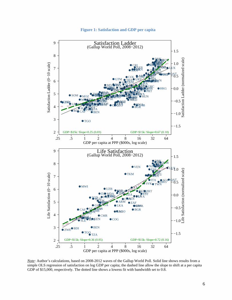
Figure 1 shows two measures of life satisfaction drawn from the Gallup World Poll: in

the top panel, we analyze responses to the “ladder of life” question, while the bottom panel

shows responses to a question about overall life satisfaction.7 The data are drawn from the five

waves of the Gallup World Poll run between 2008 and 2012 and GDP per capita, plotted on a log

scale. We have data on 155 countries, which account for over 95% of the world’s population,

across the spectrum of levels of economic development. Each of these measures of subjective

well-being is highly correlation with GDP per capita ( 0.79for the 155 countries in the upper

5 That is, the denominator in this “z-score” is the standard deviation of well-being after controlling for country

and wave fixed effects. 6 Fortunately, this issue turns out to be more troubling in theory than in practice; Stevenson and Wolfers (2008)

show alternative approaches using instead ordered probits or logits yield estimates of national happiness averages that are highly correlated ( 0.99).

7 The question analyzed in the top graph is “Please imagine a ladder with steps numbered from zero at the bottom to ten at the top. Suppose we say that the top of the ladder represents the best possible life for you, and the bottom of the ladder represents the worst possible life for you. On which step of the ladder would you say you personally feel you stand at this time, assuming that the higher the step the better you feel about your life, and the lower the step the worse you feel about it? Which step comes closest to the way you feel?” The question answered in the bottom graph is “All things considered, how satisfied are you with your life as a whole these days? Use a 0 to 10 scale, where 0 is dissatisfied and 10 is satisfied.”

5

panel, and 0.85 for the 86 countries in the lower panel) . The solid lines show the results from a

simple OLS regression, estimated for the full sample:

– log (1)

The estimated well-being–income gradient ( ) is 0.33 (se=0.02) for the ladder question and 0.44

(se=0.03) for the life satisfaction question. The figure also plots a local linear regression as a

dotted line, which allows for a non-parametric fit of the well-being–income relationship. If there

were a “satiation point,” this non-parametric fit would flatten out once basic needs were met.

Instead, the line steepens slightly among the rich nations in both graphs. Indeed, the most

striking finding is simply how closely the non-parametric fit lies to the OLS regression line. That

is, the well-being–income relationship among poor nations appears to extend roughly equally

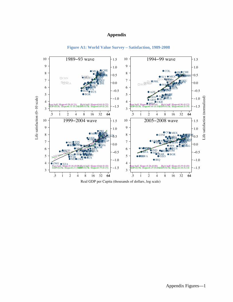
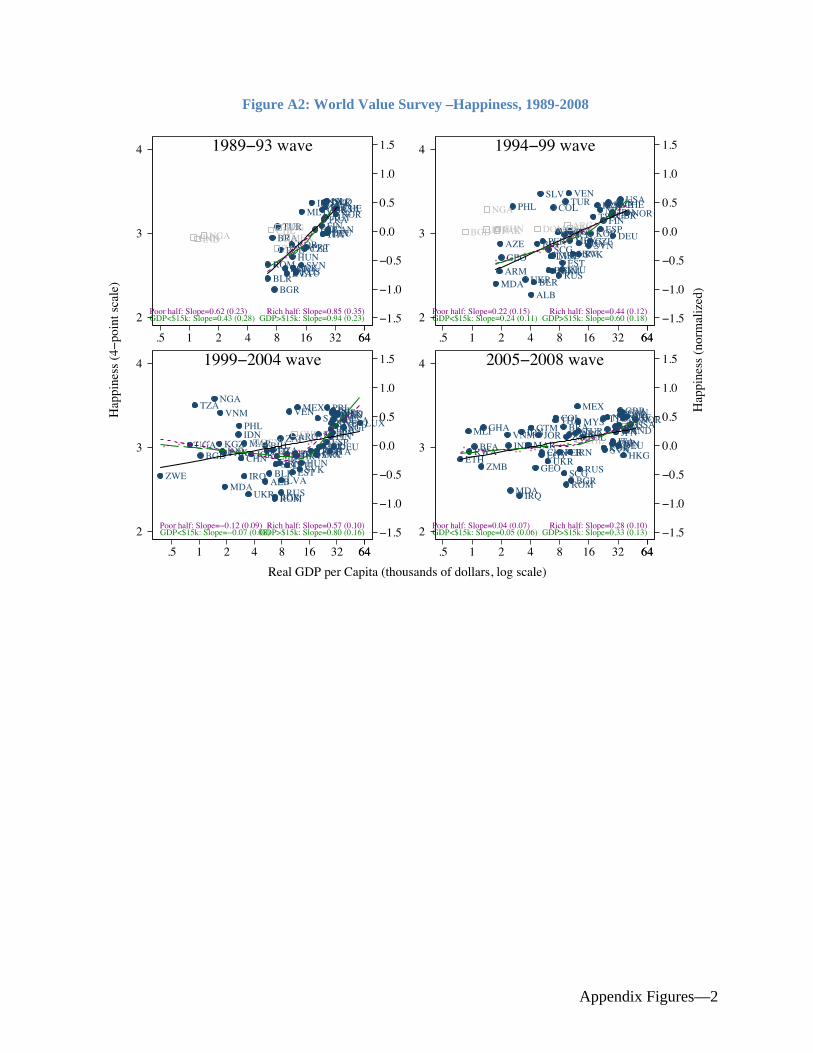
among rich nations.8 We repeat this exercise for using data from the World Values Survey for

both life satisfaction (Appendix Figure A1) and happiness (Figure A2), as well as for the

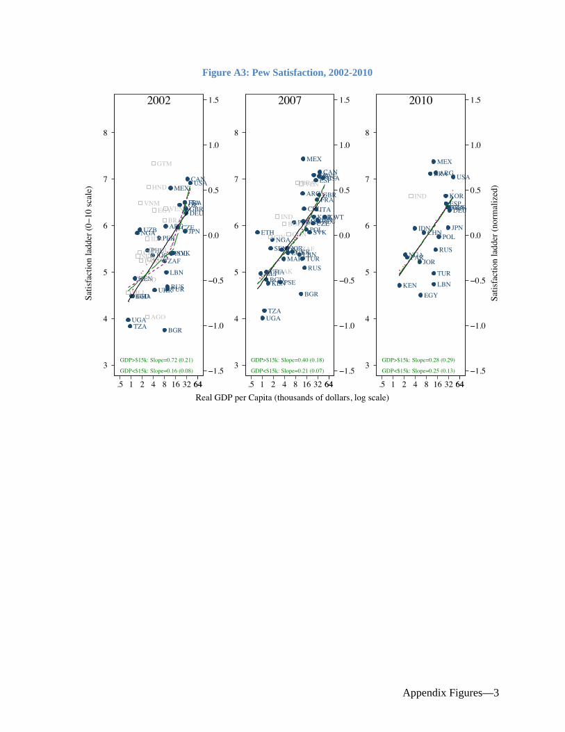
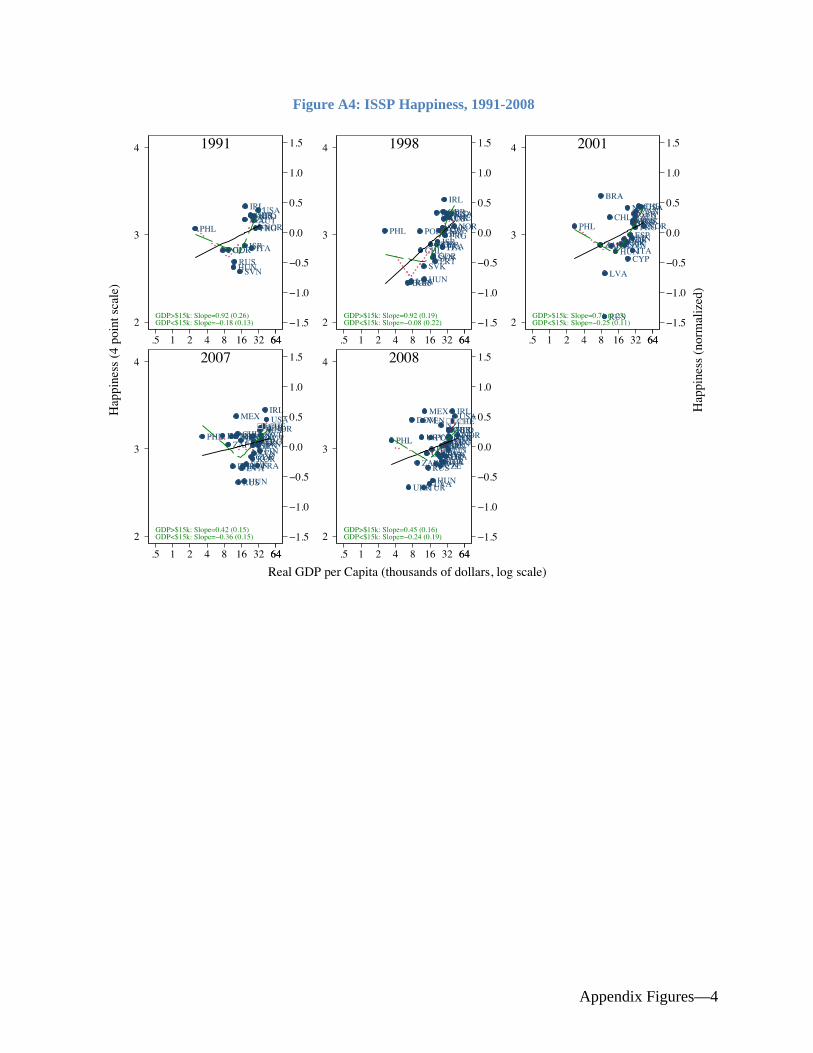
satisfaction ladder question asked in the Pew Global Attitudes Survey (Figure A3), and the 4-

point happiness question asked in the International Social Survey Program (Figure A4). In each

case, we find qualitatively similar results.

8 Deaton (2008) and Stevenson and Wolfers (2008) make similar arguments using 2006 data from the Gallup

World Poll.

6

Figure 1: Satisfaction and GDP per capita

Note: Author’s calculations, based on 2008-2012 waves of the Gallup World Poll. Solid line shows results from a simple OLS regression of satisfaction on log GDP per capita; the dashed line allow the slope to shift at a per capita GDP of $15,000, respectively. The dotted line shows a lowess fit with bandwidth set to 0.8.

AFG

AGO

ALB

ARE

ARG

ARM

AUSAUT

AZE

BDI

BEL

BEN

BFA

BGD

BGR

BHR

BIH

BLRBOL

BRA

BWA

CAF

CANCHE

CHL

CHN

CIVCMRCOD

COG

COL

COM

CRI

CYPCZE

DEU

DJI

DNK

DOMDZA

ECU

EGY

ESP

EST

ETH

FIN

FRA

GAB

GBR

GEO

GHA

GIN

GRC

GTM

HKGHNDHRV

HTI

HUN

IDN

IND

IRL

IRNIRQ

ISLISR

ITA

JAMJOR

JPNKAZ

KEN

KGZ

KHM

KOR

KWT

LAO LBN

LBR

LBY

LKA

LSO

LTU

LUX

LVAMAR

MDA

MDG

MEX

MKD

MLI

MLT

MMR

MNE

MNGMOZMRT

MUS

MWI

MYS

NER

NGANIC

NLDNOR

NPL

NZL

OMN

PAK

PAN

PER

PHL

POL

PRT

PRY

PSE

QAT

ROMRUS

RWA

SAU

SDNSEN

SGP

SLE

SLV

SOMSRB

SVKSVN

SWE

SWZ

SYRTCD

TGO

THA

TJK

TKM

TTO

TUNTUR

TWN

TZA

UGA

UKRUNK

URY

USA

UZB

VEN

VNM

YEM

ZAFZMB

ZWE

GDP>$15k: Slope=0.67 (0.10)GDP<$15k: Slope=0.25 (0.03)

−1.5

−1.0

−0.5

0.0

0.5

1.0

1.5

Satis

fact

ion

Lad

der

(nor

mal

ized

sca

le)

2

3

4

5

6

7

8

9

Satis

fact

ion

Lad

der

(0−

10 s

cale

)

.25 .5 1 2 4 8 16 32 64GDP per capita at PPP ($000s, log scale)

(Gallup World Poll, 2008−2012)

Satisfaction Ladder

AFGAGO

ARM

AUSAUT

AZE

BDI

BEL

BEN

BFA

BGD

BGR

BLR

BWACAF

CHE

CHN

CIV

CMRCOG

CYPDEU

DJI

DNK

DZAEGY

ESP

EST

FIN

FRA

GBR

GEO

GHA

HKG

IRL

IRQ

ISL

ITA

JOR

KAZ

KEN

KGZLBN

LBR

LKA

LTU

LUX

LVAMDA

MDGMLI

MLT

MOZ

MRT

MWI

NER

NGA

NLDNOR

NZL

PAK

PRT

QAT

RUS

RWASEN

SGP

SLE

SVK

SVN

SWE

SYR

TCD

TGO

TJK

TKM

TUN

TWN

TZA

UGA

UZB

VEN

VNM

ZAF

ZMB

ZWE

GDP>$15k: Slope=0.72 (0.16)GDP<$15k: Slope=0.36 (0.05)

−1.5

−1.0

−0.5

0.0

0.5

1.0

1.5

Lif

e Sa

tisfa

ctio

n (n

orm

aliz

ed s

cale

)

2

3

4

5

6

7

8

9

Lif

e Sa

tisfa

ctio

n (0

−10

sca

le)

.25 .5 1 2 4 8 16 32 64GDP per capita at PPP ($000s, log scale)

(Gallup World Poll, 2008−2012)

Life Satisfaction

7

Our more formal tests of the modified-Easterlin hypothesis come from regressions of the

form:

– log log

log log

(2)

where the subscript denotes country, the independent variables are the interaction of log real

GDP per capita with a dummy variable indicating whether GDP per capita is above or below a

cut-off level, $ . The coefficient is the well-being–income gradient among “poor”

countries (those with GDP<$k), and is the gradient among “rich” countries (those with

GDP $ ). By measuring log relative to a “cutoff,” this functional form allows for a

change in the well-being–income gradient (i.e., a “kink” in the regression line) once GDP per

capita exceeds the cutoff, but it rules out a discontinuous shift in well-being once per capita GDP

exceeds $ .9 This specification allows us to test both the “strong” version of the modified-

Easterlin hypothesis, which posits that 0, and the “weak” version, suggesting

.

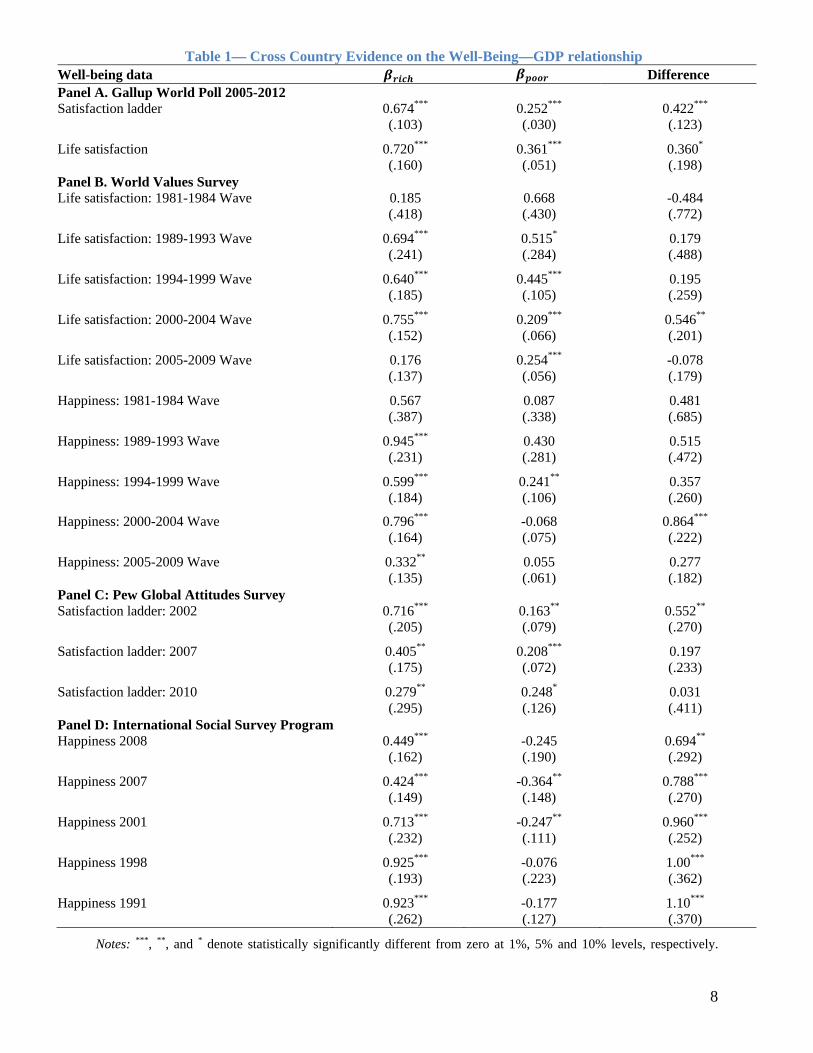
In Table 1 we report results where the cutoff level of per capita GDP, $ , is set to

$15,000.10 We repeat the results seen in Figure 1 in the first row. Subsequent rows show the

results across different questions assessing well-being and different datasets. The well-being–

income gradient in the Gallup World Poll clearly remains strong for the rich countries, and

indeed, is somewhat stronger among countries whose per capita GDP exceeds $15,000. These

data clearly reject both the weak and strong versions of the modified-Easterlin hypothesis.

9 We obtain similar results if instead we estimate the well-being–income gradient separately for rich and poor

countries. 10 Stevenson and Wolfers (2008) show estimates of ordered probit regressions estimating the well-being income

gradient for incomes above and below $15,000, while Deaton (2008) tested thresholds of $12,000 and $20,000. Table 2 shows the results using alternative thresholds of $8,000 and $25,000, as well as the median level of GDP for the sample.

8

Table 1— Cross Country Evidence on the Well-Being—GDP relationship

Notes: ***, **, and * denote statistically significantly different from zero at 1%, 5% and 10% levels, respectively.

Well-being data Difference Panel A. Gallup World Poll 2005-2012 Satisfaction ladder 0.674*** 0.252*** 0.422***

(.103) (.030) (.123)

Life satisfaction 0.720*** 0.361*** 0.360*

(.160) (.051) (.198)Panel B. World Values Survey Life satisfaction: 1981-1984 Wave 0.185 0.668 -0.484

(.418) (.430) (.772)

Life satisfaction: 1989-1993 Wave 0.694*** 0.515* 0.179

(.241) (.284) (.488)

Life satisfaction: 1994-1999 Wave 0.640*** 0.445*** 0.195

(.185) (.105) (.259)

Life satisfaction: 2000-2004 Wave 0.755*** 0.209*** 0.546**

(.152) (.066) (.201)

Life satisfaction: 2005-2009 Wave 0.176 0.254*** -0.078

(.137) (.056) (.179)

Happiness: 1981-1984 Wave 0.567 0.087 0.481

(.387) (.338) (.685)

Happiness: 1989-1993 Wave 0.945*** 0.430 0.515

(.231) (.281) (.472)

Happiness: 1994-1999 Wave 0.599*** 0.241** 0.357

(.184) (.106) (.260)

Happiness: 2000-2004 Wave 0.796*** -0.068 0.864***

(.164) (.075) (.222)

Happiness: 2005-2009 Wave 0.332** 0.055 0.277 (.135) (.061) (.182)Panel C: Pew Global Attitudes Survey Satisfaction ladder: 2002 0.716*** 0.163** 0.552**

(.205) (.079) (.270)

Satisfaction ladder: 2007 0.405** 0.208*** 0.197

(.175) (.072) (.233)

Satisfaction ladder: 2010 0.279** 0.248* 0.031 (.295) (.126) (.411)Panel D: International Social Survey ProgramHappiness 2008 0.449*** -0.245 0.694**

(.162) (.190) (.292)

Happiness 2007 0.424*** -0.364** 0.788***

(.149) (.148) (.270)

Happiness 2001 0.713*** -0.247** 0.960***

(.232) (.111) (.252)

Happiness 1998 0.925*** -0.076 1.00***

(.193) (.223) (.362)

Happiness 1991 0.923*** -0.177 1.10***

(.262) (.127) (.370)

9

The next ten rows repeat the analysis using five rounds of the World Values Survey for

both a life satisfaction question which mirrors that in the Gallup World Poll, and a question on

happiness. The results roughly parallel those above, albeit with less statistical power.11

In seven of the ten rows we can reject the strong claim that 0. In two cases

and are statistically significantly different from each other, however the well-being–

income relationship is steeper among rich countries than the poor. Indeed, in all but two cases,

the estimate of actually exceeds that for (rather than the other way around). In the

two cases in which the point estimate of is larger, we cannot reject the null that

.

There are two other useful cross-country studies that are worth analyzing, the Pew Global

Attitudes studies, which posed the satisfaction ladder question in 44 countries in 2002, 47

countries in 2007, and 22 countries in 2010, and the International Social Survey Program, which

asked a consistent happiness question in 1991, 1998, 2001, 2007 and 2008 (plotted in Appendix

Figures A3 and A4). Each of these datasets strongly reject the null that 0. Moreover, to

the extent that the well-being–income relationship changes, it appears stronger for rich countries.

Somewhat paradoxically, the ISSP data appear to show a negative well-being–income gradient

among poor nations, but this is entirely due to a single influential observation, the Philippines

(whose influence is even greater given that these samples contain mostly medium- and high-

income countries).

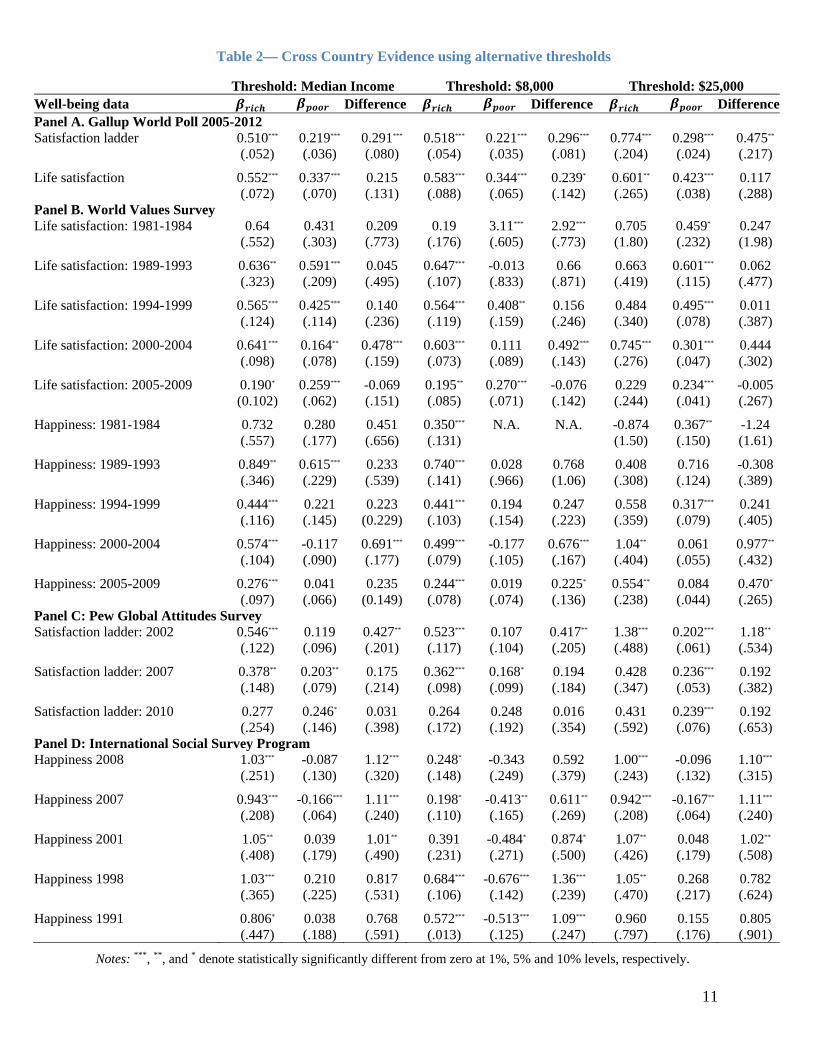
In Table 2 we consider alternative thresholds for “poor” and “rich”. In the first three

columns we consider differences between below and above median income countries. In the next

11 In several countries the surveys were not nationally representative, focusing instead on urban areas and more

educated members of society. Our anaylsis drops highly unrepresentative observations as detailed in Stevenson and Wolfers (2008) and Sacks, Stevenson, and Wolfers (2013).

10

three we use an $8,000 threshold such that poor countries are those with GDP per capita below

$8,000. Finally, in the last three columns we consider a higher income threshold of $25,000. In

these alternative specifications, most of the estimates of are statistically significantly

different from zero and we remain unable to reject the null that in most of our

samples. For the estimates in which and are statistically significantly different from

each other, in all but one case the estimate of exceeds that for .

In sum, comparisons of average levels of subjective well-being and GDP per capita across

countries suggest that the well-being–income relationship observed among poor countries holds

in at least equal measure among rich countries. In the few cases where we cannot reject

0, we also cannot reject . Our larger datasets emphatically reject the weak and

strong forms of the modified-Easterlin hypothesis, while the smaller samples are sufficiently

imprecise as to provide no statistically significant evidence in support of (or against) it.

11

Table 2— Cross Country Evidence using alternative thresholds

Notes: ***, **, and * denote statistically significantly different from zero at 1%, 5% and 10% levels, respectively.

Threshold: Median Income Threshold: $8,000 Threshold: $25,000 Well-being data Difference Difference DifferencePanel A. Gallup World Poll 2005-2012 Satisfaction ladder 0.510*** 0.219*** 0.291*** 0.518*** 0.221*** 0.296*** 0.774*** 0.298*** 0.475**

(.052) (.036) (.080) (.054) (.035) (.081) (.204) (.024) (.217)

Life satisfaction 0.552*** 0.337*** 0.215 0.583*** 0.344*** 0.239* 0.601** 0.423*** 0.117 (.072) (.070) (.131) (.088) (.065) (.142) (.265) (.038) (.288) Panel B. World Values Survey Life satisfaction: 1981-1984 0.64 0.431 0.209 0.19 3.11*** 2.92*** 0.705 0.459* 0.247

(.552) (.303) (.773) (.176) (.605) (.773) (1.80) (.232) (1.98)

Life satisfaction: 1989-1993 0.636** 0.591*** 0.045 0.647*** -0.013 0.66 0.663 0.601*** 0.062

(.323) (.209) (.495) (.107) (.833) (.871) (.419) (.115) (.477)

Life satisfaction: 1994-1999 0.565*** 0.425*** 0.140 0.564*** 0.408** 0.156 0.484 0.495*** 0.011

(.124) (.114) (.236) (.119) (.159) (.246) (.340) (.078) (.387)

Life satisfaction: 2000-2004 0.641*** 0.164** 0.478*** 0.603*** 0.111 0.492*** 0.745*** 0.301*** 0.444

(.098) (.078) (.159) (.073) (.089) (.143) (.276) (.047) (.302)

Life satisfaction: 2005-2009 0.190* 0.259*** -0.069 0.195** 0.270*** -0.076 0.229 0.234*** -0.005

(0.102) (.062) (.151) (.085) (.071) (.142) (.244) (.041) (.267)

Happiness: 1981-1984 0.732 0.280 0.451 0.350*** N.A. N.A. -0.874 0.367** -1.24

(.557) (.177) (.656) (.131) (1.50) (.150) (1.61)

Happiness: 1989-1993 0.849** 0.615*** 0.233 0.740*** 0.028 0.768 0.408 0.716 -0.308

(.346) (.229) (.539) (.141) (.966) (1.06) (.308) (.124) (.389)

Happiness: 1994-1999 0.444*** 0.221 0.223 0.441*** 0.194 0.247 0.558 0.317*** 0.241

(.116) (.145) (0.229) (.103) (.154) (.223) (.359) (.079) (.405)

Happiness: 2000-2004 0.574*** -0.117 0.691*** 0.499*** -0.177 0.676*** 1.04** 0.061 0.977**

(.104) (.090) (.177) (.079) (.105) (.167) (.404) (.055) (.432)

Happiness: 2005-2009 0.276*** 0.041 0.235 0.244*** 0.019 0.225* 0.554** 0.084 0.470* (.097) (.066) (0.149) (.078) (.074) (.136) (.238) (.044) (.265) Panel C: Pew Global Attitudes Survey Satisfaction ladder: 2002 0.546*** 0.119 0.427** 0.523*** 0.107 0.417** 1.38*** 0.202*** 1.18**

(.122) (.096) (.201) (.117) (.104) (.205) (.488) (.061) (.534)

Satisfaction ladder: 2007 0.378** 0.203** 0.175 0.362*** 0.168* 0.194 0.428 0.236*** 0.192

(.148) (.079) (.214) (.098) (.099) (.184) (.347) (.053) (.382)

Satisfaction ladder: 2010 0.277 0.246* 0.031 0.264 0.248 0.016 0.431 0.239*** 0.192 (.254) (.146) (.398) (.172) (.192) (.354) (.592) (.076) (.653) Panel D: International Social Survey Program Happiness 2008 1.03*** -0.087 1.12*** 0.248* -0.343 0.592 1.00*** -0.096 1.10***

(.251) (.130) (.320) (.148) (.249) (.379) (.243) (.132) (.315)

Happiness 2007 0.943*** -0.166*** 1.11*** 0.198* -0.413** 0.611** 0.942*** -0.167** 1.11***

(.208) (.064) (.240) (.110) (.165) (.269) (.208) (.064) (.240)

Happiness 2001 1.05** 0.039 1.01** 0.391 -0.484* 0.874* 1.07** 0.048 1.02**

(.408) (.179) (.490) (.231) (.271) (.500) (.426) (.179) (.508)

Happiness 1998 1.03*** 0.210 0.817 0.684*** -0.676*** 1.36*** 1.05** 0.268 0.782

(.365) (.225) (.531) (.106) (.142) (.239) (.470) (.217) (.624)

Happiness 1991 0.806* 0.038 0.768 0.572*** -0.513*** 1.09*** 0.960 0.155 0.805 (.447) (.188) (.591) (.013) (.125) (.247) (.797) (.176) (.901)

12

II. Within-Country Cross-Sectional Comparisons

We now turn to analyzing the relationship between well-being and income that one

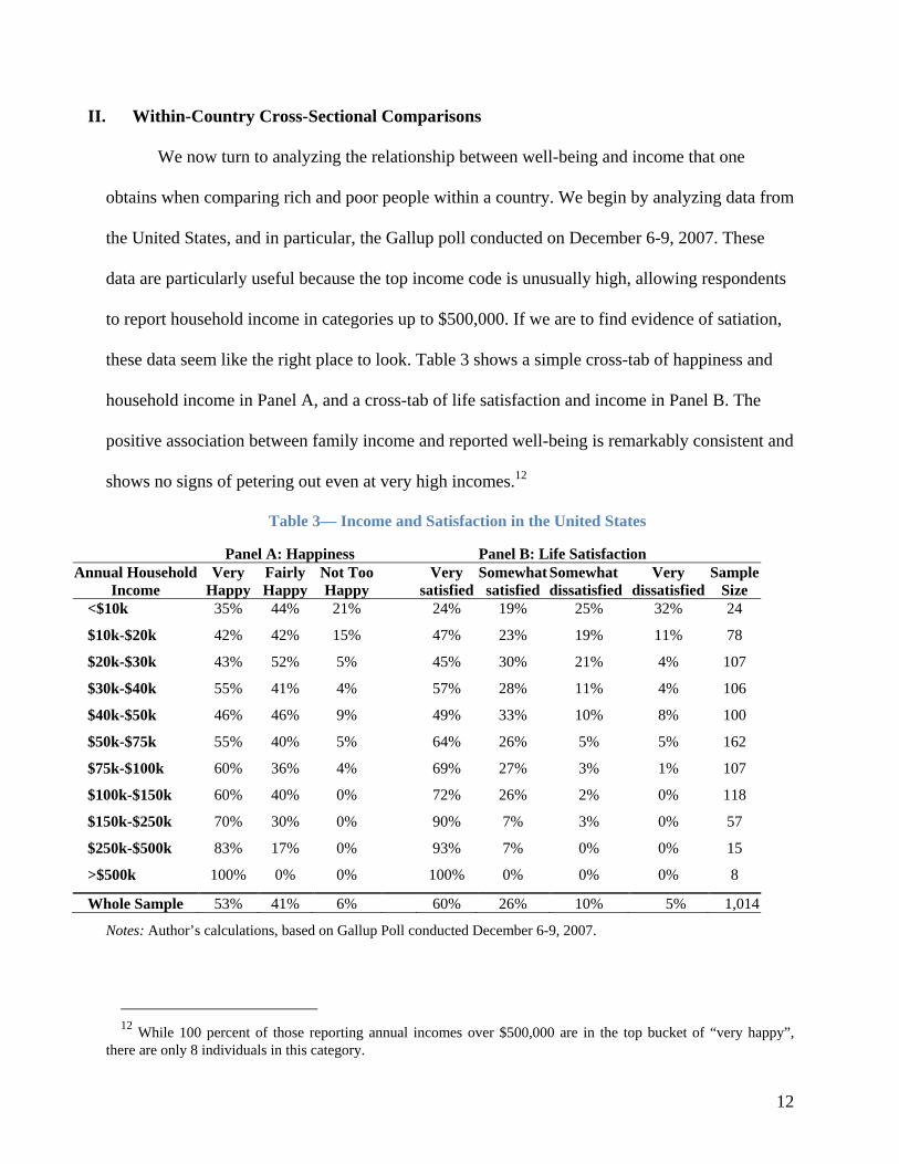
obtains when comparing rich and poor people within a country. We begin by analyzing data from

the United States, and in particular, the Gallup poll conducted on December 6-9, 2007. These

data are particularly useful because the top income code is unusually high, allowing respondents

to report household income in categories up to $500,000. If we are to find evidence of satiation,

these data seem like the right place to look. Table 3 shows a simple cross-tab of happiness and

household income in Panel A, and a cross-tab of life satisfaction and income in Panel B. The

positive association between family income and reported well-being is remarkably consistent and

shows no signs of petering out even at very high incomes.12

Table 3— Income and Satisfaction in the United States

Panel A: Happiness Panel B: Life Satisfaction Annual Household

Income Very

Happy Fairly Happy

Not Too Happy

Very satisfied

Somewhatsatisfied

Somewhat dissatisfied

Very dissatisfied

Sample Size

<$10k 35% 44% 21% 24% 19% 25% 32% 24

$10k-$20k 42% 42% 15% 47% 23% 19% 11% 78

$20k-$30k 43% 52% 5% 45% 30% 21% 4% 107

$30k-$40k 55% 41% 4% 57% 28% 11% 4% 106

$40k-$50k 46% 46% 9% 49% 33% 10% 8% 100

$50k-$75k 55% 40% 5% 64% 26% 5% 5% 162

$75k-$100k 60% 36% 4% 69% 27% 3% 1% 107

$100k-$150k 60% 40% 0% 72% 26% 2% 0% 118

$150k-$250k 70% 30% 0% 90% 7% 3% 0% 57

$250k-$500k 83% 17% 0% 93% 7% 0% 0% 15

>$500k 100% 0% 0% 100% 0% 0% 0% 8

Whole Sample 53% 41% 6% 60% 26% 10% 5% 1,014

Notes: Author’s calculations, based on Gallup Poll conducted December 6-9, 2007.

12 While 100 percent of those reporting annual incomes over $500,000 are in the top bucket of “very happy”,

there are only 8 individuals in this category.

13

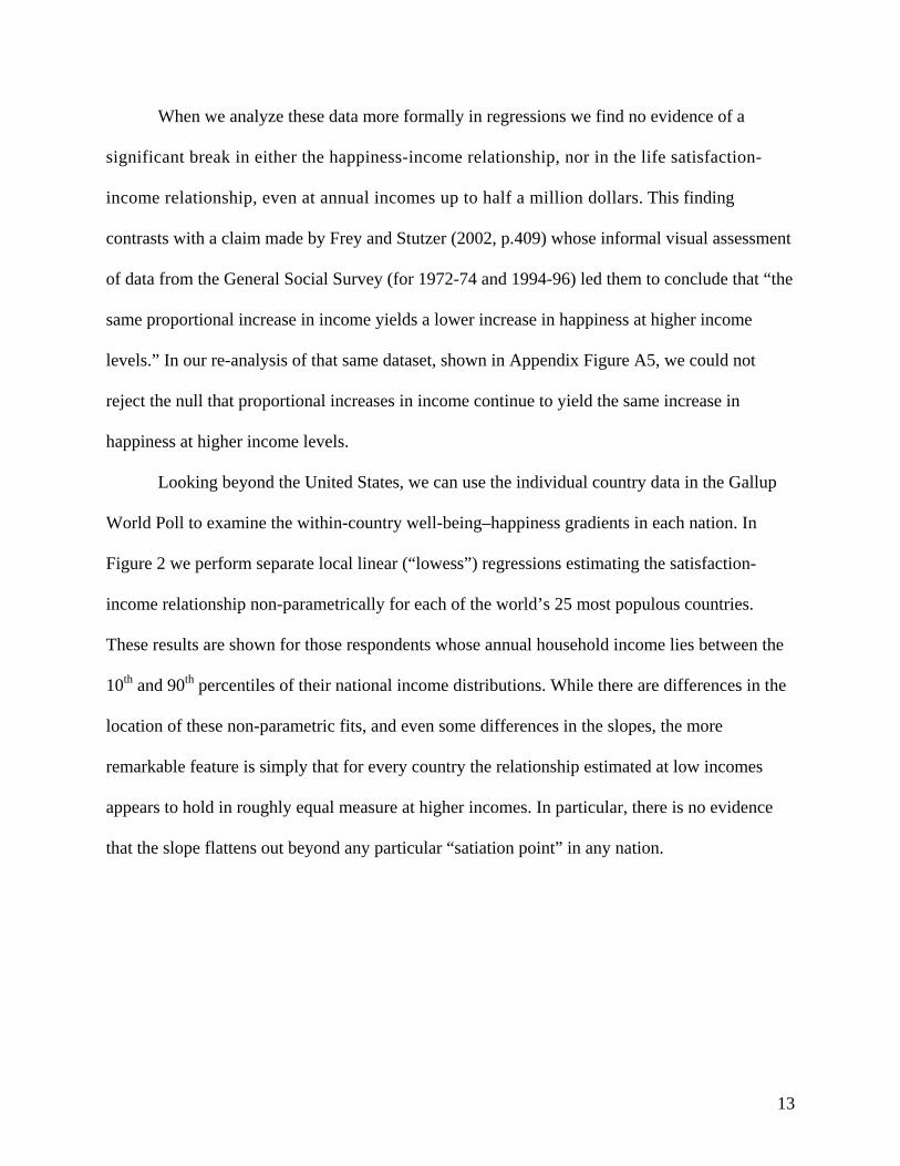
When we analyze these data more formally in regressions we find no evidence of a

significant break in either the happiness-income relationship, nor in the life satisfaction-

income relationship, even at annual incomes up to half a million dollars. This finding

contrasts with a claim made by Frey and Stutzer (2002, p.409) whose informal visual assessment

of data from the General Social Survey (for 1972-74 and 1994-96) led them to conclude that “the

same proportional increase in income yields a lower increase in happiness at higher income

levels.” In our re-analysis of that same dataset, shown in Appendix Figure A5, we could not

reject the null that proportional increases in income continue to yield the same increase in

happiness at higher income levels.

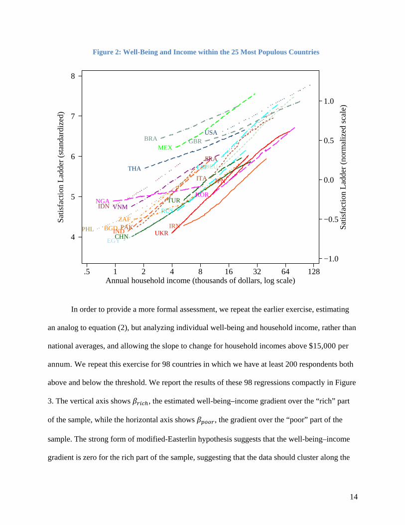
Looking beyond the United States, we can use the individual country data in the Gallup

World Poll to examine the within-country well-being–happiness gradients in each nation. In

Figure 2 we perform separate local linear (“lowess”) regressions estimating the satisfaction-

income relationship non-parametrically for each of the world’s 25 most populous countries.

These results are shown for those respondents whose annual household income lies between the

10th and 90th percentiles of their national income distributions. While there are differences in the

location of these non-parametric fits, and even some differences in the slopes, the more

remarkable feature is simply that for every country the relationship estimated at low incomes

appears to hold in roughly equal measure at higher incomes. In particular, there is no evidence

that the slope flattens out beyond any particular “satiation point” in any nation.

14

Figure 2: Well-Being and Income within the 25 Most Populous Countries

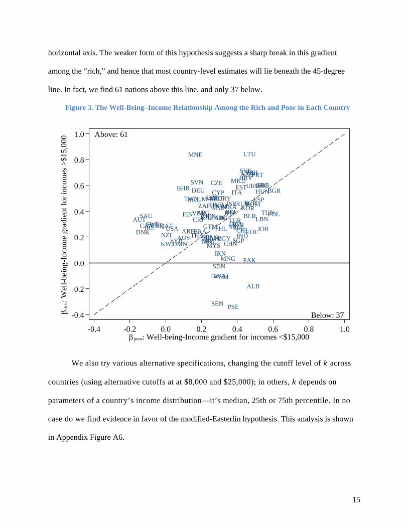
In order to provide a more formal assessment, we repeat the earlier exercise, estimating

an analog to equation (2), but analyzing individual well-being and household income, rather than

national averages, and allowing the slope to change for household incomes above $15,000 per

annum. We repeat this exercise for 98 countries in which we have at least 200 respondents both

above and below the threshold. We report the results of these 98 regressions compactly in Figure

3. The vertical axis shows , the estimated well-being–income gradient over the “rich” part

of the sample, while the horizontal axis shows , the gradient over the “poor” part of the

sample. The strong form of modified-Easterlin hypothesis suggests that the well-being–income

gradient is zero for the rich part of the sample, suggesting that the data should cluster along the

CHNIND

USA

IDN

BRA

PAKBGD

NGA

RUS

JPN

MEX

PHL

VNM

DEU

EGY

TUR

IRN

THA

FRA

GBR

ITA

ZAF

KOR

ESP

UKR

−1.0

−0.5

0.0

0.5

1.0

Satis

fact

ion

Lad

der

(nor

mal

ized

sca

le)

4

5

6

7

8

Satis

fact

ion

Lad

der

(sta

ndar

dize

d)

.5 1 2 4 8 16 32 64 128Annual household income (thousands of dollars, log scale)

15

horizontal axis. The weaker form of this hypothesis suggests a sharp break in this gradient

among the “rich,” and hence that most country-level estimates will lie beneath the 45-degree

line. In fact, we find 61 nations above this line, and only 37 below.

Figure 3. The Well-Being–Income Relationship Among the Rich and Poor in Each Country

We also try various alternative specifications, changing the cutoff level of across

countries (using alternative cutoffs at at $8,000 and $25,000); in others, depends on

parameters of a country’s income distribution—it’s median, 25th or 75th percentile. In no

case do we find evidence in favor of the modified-Easterlin hypothesis. This analysis is shown

in Appendix Figure A6.

AFG

ALB

ARE

ARG

AUS

AUT

AZE

BEL

BGRBHR

BIH

BLR

BOLBRA

BWA

CANCHL

CHN

COLCOM

CRI

CYP

CZEDEU

DJIDNK

DOM

DZA

ECU

EGY

ESP

EST

FINFRAGAB

GBR

GRC

GTM

HKGHND

HRV

HUN

INDIRL

IRN

ISR

ITA

JOR

JPNKAZ

KOR

KWT

LBN

LTU

LVA

MAR

MEX

MKD

MLT

MNE

MNG

MRTMYS

NICNZL

OMN

PAK

PAN

PERPHL

POL

PRT

PRY

PSE

QAT

ROMRUS

SAU

SDN

SEN

SGP

SRB

SVK

SVN

SWE

SYRTHA

TJKTUN

TUR

TWN

UKR

URY

USA

UZB

VEN

VNM

ZAF

Above: 61

Below: 37-0.4

-0.2

0.0

0.2

0.4

0.6

0.8

1.0

ric

h: W

ell-

bein

g-In

com

e gr

adie

nt f

or in

com

es >

$15,

000

-0.4 -0.2 0.0 0.2 0.4 0.6 0.8 1.0poor: Well-being-Income gradient for incomes <$15,000

16

III. Conclusions

While the idea that there is some critical level of income beyond which income no longer

impacts well-being is intuitively appealing, it is at odds with the data. As we have shown, there is

no major well-being dataset that supports this commonly made claim. To be clear, our analysis in

this paper has been confined to the sorts of evaluative measures of life satisfaction and happiness

that have been the focus of proponents of the (modified) Easterlin hypothesis. In an interesting

recent contribution, Kahneman and Deaton (2010) have shown that in the United States, people

earning above $75,000 do not appear to enjoy either more positive affect nor less negative affect

than those earning just below that. We are intrigued by these findings, although we conclude by

noting that they are based on very different measures of well-being, and so they are not

necessarily in tension with our results. Indeed, those authors also find no satiation point for

evaluative measures of well-being.

References—1

IV References

Clark, Andrew E., Paul Frijters, and Michael A. Shields. "Relative Income, Happiness and Utility: An Explanation for the Easterlin Paradox and Other Puzzles." Journal of Economic Literature 46, no. 1 (2008): 95-144. Deaton, Angus "Income, Health, and Well-Being around the World: Evidence from the Gallup World Poll." Journal of Economic Perspectives, 2008 22(2), pp. 53-72. Di Tella, Rafael, and Robert MacCulloch. Happiness Adaptation to Income beyond "Basic Needs". NBER Working Paper, National Bureau of Economic Research, 2008. Diener, Ed, and Martin E.P. Seligman. "Beyond money: Toward an economy of well-being." Psychological Science in the Public Interest 5 (2004): 1-31. Easterlin, Richard A. "Does economic growth improve the human lot? Some empirical evidence." In Nations and Households in Economic Growth: Essays in Honor of Moses Abramowitz, by Paul A David and Melvin W. Reder. New York: Academic Press, Inc., 1974. Easterlin, Richard A., and Onnicha Sawangfa. Happiness and Economic Growth: Does the Cross Section Predict Time Trends? Evidence from Developing Countries. mimeo, University of Southern California, 2009. Frey, Bruno S., and Alois Stutzer. "What Can Economists Learn from Happiness Research?" Journal of Economic Literature 40 (2002): 402-435. Kahneman, Daniel and Angus Deaton. “High Income Improves Evaluation of Life But Not Emotional Well-Being” Proceedings of the National Academy of Sciences, September 7 2010, 107(38) 16489-16493. Layard, Richard. "Happiness: Has Social Science a Clue." Lionel Robbins Memorial Lectures 2002/3. London School of Economics, 2003.

—. Happiness: Lessons from a New Science. London: Penguin, 2005.

Oswald, Andrew J. "On the Curvature of the Reporting Function from Objective Reality to Subjective Feelings." Economics Letters, 2008. Sacks, Daniel, Betsey Stevenson, and Justin Wolfers “The New Stylized Facts About Income and Subjective Well-being”, Emotion, Dec 2012, 12 (6): 1181-1187 Sacks, Daniel, Betsey Stevenson, and Justin Wolfers “Growth in Subjective Well-being and Income over Time”, 2013 mimeo. Stevenson, Betsey, and Justin Wolfers. "Economic Growth and Happiness: Reassessing the Easterlin Paradox." Brookings Papers on Economic Activity, Spring 2008: 1-87

Appendix Figures—1

Appendix

Figure A1: World Value Survey – Satisfaction, 1989-2008

Appendix Figures—2

Figure A2: World Value Survey –Happiness, 1989-2008

Appendix Figures—3

Figure A3: Pew Satisfaction, 2002-2010

Appendix Figures—4

Figure A4: ISSP Happiness, 1991-2008

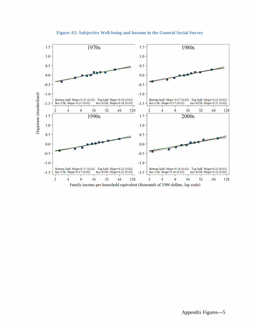
Appendix Figures—5

Figure A5: Subjective Well-being and Income in the General Social Survey

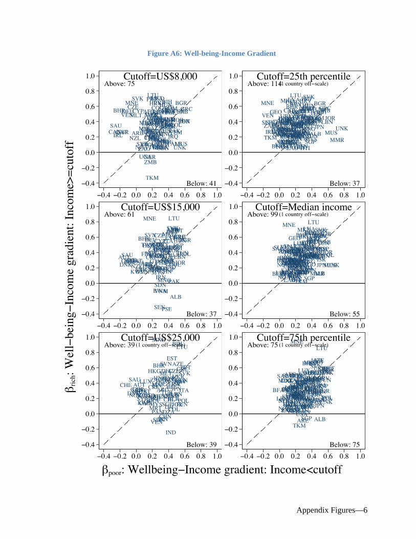
Appendix Figures—6

Figure A6: Well-being-Income Gradient