Subjective Probability as Sampling Propensity∗(To appear in Review of Philosophy and Psychology)

Thomas F. Icard, IIIStanford University

AbstractSubjective probability plays an increasingly important role in many fields concerned with human cognition and

behavior. Yet there have been significant criticisms of the idea that probabilities could actually be represented in themind. This paper presents and elaborates a view of subjective probability as a kind of sampling propensity associatedwith internally represented generative models. The resulting view answers to some of the most well known criticismsof subjective probability, and is also supported by empirical work in neuroscience and behavioral psychology. Therepercussions of the view for how we conceive of many ordinary instances of subjective probability, and how it relatesto more traditional conceptions of subjective probability, are discussed in some detail.

1 IntroductionSubjective probability is a ubiquitous tool in philosophy, psychology, the social sciences, and elsewhere, for under-standing aspects of intelligent inference, reasoning, and decision making under uncertainty. The basic idea is thatnumerical probabilities, in the familiar mathematical sense, can be used to represent a person’s subjective “strength”or “degree” of conviction or belief. There is no general consensus about what exactly these numbers mean, and how(if at all) they might be literally represented in an agent’s mind, though there are some classic analyses of the con-cept of probability. Foundational discussions of subjective probability, beginning with Ramsey, de Finetti, and others,typically analyze or define the concept of subjective probability by reducing it to some observable or measurable phe-nomenon, such as preference or betting odds. As Ramsey famously put it, “a degree of belief is a causal property ofit, which we can express vaguely as the extent to which we are prepared to act on it” (Ramsey, 1931, 71).

While these concepts of probability—tied intimately to behavioral dispositions of a whole person—may be usefulfor many purposes, they are not evidently appropriate to explain the role that subjective probability plays in contempo-rary psychology and cognitive science. In much of this work, especially recently, the proposal is not just that we canreasonably ascribe subjective probabilities to people, and thereby explain much of their behavior. There is a furtherclaim that the brain somehow encodes probabilities and uses these in the service of prediction and action selection (forexample, see Knill and Pouget 2004; Gopnik et al. 2004; Chater et al. 2006; Yang and Shadlen 2007; Vilares and Kord-ing 2011; Perfors 2012; Clark 2013, among many others); that is, something like subjective probabilities are assumedto play a direct causal role in pervasive mental computations. While much of this work is about low-level cognition,especially perception, increasingly more work is aimed at ordinary inference and prediction about “everyday” eventsand topics (see, e.g., Griffiths and Tenenbaum 2006; Goodman et al. 2014, inter alia), thus coming quite close tothe sorts of commonplace inferences and judgments that are the focus of many philosophers interested in subjectiveprobability and its associated normative questions. Given the increasing prevalence of probability in computationalmodeling of cognition, it is important to understand both (1) what, concretely, the relevant states of mind are supposedto be, and (2) how the resulting notion of subjective probability relates to the more traditional conceptions.

In this paper we present, explain, elaborate, and aim to elucidate a recently proposed hypothesis about how prob-abilities might be concretely represented. The Sampling Hypothesis asserts that an important way in which the brain∗This is a preprint. The final version will appear in Review of Philosophy and Psychology. Thanks to the RoPP editor Paul Egre, to the journal

reviewers, and to Falk Lieder for useful comments that helped improve the paper. Thanks also to Wesley Holliday, Shane Steinert-Threlkeld, andmy dissertation committee (see Icard 2013) for helpful comments on an earlier version.

1

represents probabilistic information is via generative models whose underlying “sampling propensities” implicitly en-code probabilities for possible states of the world. That is, a person’s subjective probabilities for a given event areencoded roughly by the proportion of times the person’s “intuitive model” of the world would be expected to samplethat event from among the possible outputs of the model. In other words, we replace Ramsey’s propensity to actwith an internal sampling propensity of the person’s intuitive model, effectively reducing subjective probabilities to aparticular kind of (at least relatively) objective probability.

The Sampling Hypothesis has received some impressive empirical support over the last several years, and the cog-nitive and neuroscientific literature on this topic is complex and growing. This paper will not contain a comprehensivesurvey. Instead, the aim is to give a general sense of the empirical support for the hypothesis, to make a convincingcase that there is something to the hypothesis, and to explore some of the consequences of the overall view for how weshould think about subjective probability. Rather than replacing more traditional analyses of subjective probability, theintention is to understand an important variety of subjective probability that can play a different theoretical role, onemore appropriate to its use in psychology, and perhaps also in much of philosophy, by capturing part of what guidesour everyday inferences, predictions, judgments, and actions.

The outline of the paper is as follows. In §2 we offer some background discussion about the concept of subjectiveprobability, what theoretical role it is supposed to play in the psychological and behavioral sciences and in philosophy,and what we take to be the conceptual core of subjective probability. In §3 and §4 we review commonly expresseddoubts about the very idea that the mind could harbor numerical probabilistic representations. In §5 we introducethe proposal in detail (with some mathematical details left to Appendix A), and offer clarificatory remarks in §6 and§7. Important empirical evidence—centered around neural computation, heuristics and biases, and the phenomenonof probability matching—is reviewed and discussed in §8, §9, §10, and Appendix B. Challenges to the hypothesis arepresented in §11, and a final comparison with the traditional conceptions of subjective probability is offered in §12.

Our goal is not to convince the reader that the Sampling Hypothesis must be correct, but rather to offer a proposalabout what exactly the hypothesis comes to, and show why it is a promising, attractive idea worth taking seriously.

2 Analyzing Subjective ProbabilityThe standard formalization of probability theory assumes a sample space V , together with some non-trivial sigma-algebra E over V , and a measurable function P : E→ [0,1] satisfying the usual axioms of (at least finite) additivity andnormalization (that P(V ) = 1). The framework can be analyzed and applied with the basic mathematical entities—inparticular the probabilities over “events” in E—interpreted in numerous ways. For instance, on a frequency interpreta-tion, the probability values describe objective (limiting) frequencies of events in the world, relative to some backgroundreference class. On a propensity interpretation, probabilities describe real dispositions or objective physical tenden-cies. One of the most important interpretations for the behavioral and social sciences is the subjective interpretation,according to which these probabilities represent a “degree of confidence” or some other measure of how likely thingsare from a specific agent’s subjective point of view. The following are some examples of typical phenomena to whichthe probability calculus, under a subjective interpretation, has been applied:

1. A government must decide whether, and how much, to invest in R&D on alternative energy.

2. A doctor is trying to decide whether to prescribe rest or a penicillin shot for a patient with a soar throat.

3. Seeing a cloudy sky, a person must decide whether to walk home and risk rain, or take the bus.

4. An interlocutor must determine whether a speaker is talking about a person named ‘Paris’ or a city of that name.

5. A monkey must “decide” whether to saccade to the left or right, in order to receive a payoff.

6. The visual system must determine how far an object is, given a pattern of input on the retina.

This short list is already quite diverse. In scenarios like 1 and 2 (and perhaps 3), many claim that the probabilitycalculus (together with a theory of utility, and perhaps other ingredients) plays into a compelling normative accountof what one ought to do. After assessing the situation, figuring out what the possible actions and outcomes might be,

2

and assigning probabilities to different eventualities in a way consistent with the probability axioms, one ought assessactions by calculating their expected utilities and choosing one whose expected utility is non-dominated. In 4-6 (andperhaps 3), by contrast, the claim is typically that our brains somehow calculate probabilities “for us,” and that therelevant computations are happening “under the hood,” so to speak, not under conscious control. Despite this diversity,in all of these cases, the probabilities in question—whether concerning possible advances in energy development, whatentity a speaker is likely to be referring to, or spatial distances—have been understood as subjective. In advance ofany further conceptual analysis of subjective probability, we would like to offer a rough characterization of the core ofwhat the different uses of subjective probability have in common, across these disciplines that invoke the notion:

(A) The event space E and the probability values should capture an agent’s subjective “viewpoint” on the world;that is, how possibilities “look” from the perspective of the agent, with regard to their (relative) plausibility.

(B) The probability values should be in some way responsive to data or evidence.

(C) Probabilities should combine with some notion of utility or desirability to guide the agent’s actions and choices,and perhaps more generally play a role in the agent’s practical reasoning (viz. planning, etc.).

Beyond this common core, a number of authors have offered further analyses and definitions of subjective probability.1

Many attempt to reduce the concept to some more primitive or easily understood (or measured) phenomenon, and inparticular to some kind of behavior, or behavioral disposition. We can identify three important and influential analysesof this sort. First, a very common and prominent proposal has been to establish conditions on preference relations—e.g., over gambles, or relative likelihood statements—such that any agent with preferences satisfying such-and-suchconditions can be represented as harboring certain subjective probability judgments (Ramsey 1931, Savage 1954,Anscombe and Aumann 1963 are classic examples). The agent’s probabilities can then be identified with one ofthese representing probability functions. A second proposal is to identify an agent’s probabilities with their bettingquotients: roughly, the odds on bets involving elements of E that the agent deems fair (de Finetti, 1974). This construalplays naturally into the so called Dutch book argument for justifying the standard probability axioms for subjectiveprobability. A third view, defended in different ways by both Lewis (1974) and Davidson (1975), claims subjectiveprobabilities form part of a rational reconstruction by an interpreter, of what guides an agent’s overall behavior.The interpreter observes the agent’s actions and choices, and ascribes probabilities and utilities that most effectivelyrationalize these actions and choices, under the assumption that she is maximizing her expected utility.

All of these proposals make good on (A)-(C), but go beyond this conceptual core in saying exactly what theoreticalrole subjective probability is meant to play, including how it is to be measured or determined. While these proposalsmay work for characterizing scenarios like 1 and 2 above,2 they are arguably less promising as characterizations of therelevant states in examples like 4, 5 and 6. Monkey brains do not literally assess fairness of bets, and the visual systemdoes not express preferences over a rich set of gambles. Moreover, even if we could somehow apply these frameworksto the mechanisms in question, it is not obvious that the probabilities thus obtained would coincide with what in factexplains how these mechanisms work, that is, how in fact the brain uses probabilistic representations to produce thebehaviors in question, if it does. The proposals mentioned above all have the advantage that they can be applied evenin cases where probabilities are nowhere explicitly represented in the agent’s mind. Subjective probabilities can beconstructed and ascribed in any case where an agent exhibits behavior of the requisite kind, quite independent of whatis going on in the agent’s mind. However, this flexibility is a potential downside when we suspect that perhaps thebrain does incorporate probabilistic representation—we then want to understand these representations as such.

What is a useful concept of subjective probability for the purpose of cognitive science and psychology, wherewe are interested in how, concretely, the human mind copes with uncertainty? We claim that further analysis of theconcept itself, beyond (A)-(C), is unnecessary. If we can find a psychological phenomenon that is properly modeled

1(C) is usually, but not always, made explicit in analyses of probability. As many have argued (e.g., James 1890; Ramsey 1931; Williamson2015, etc.), a notion of idle belief, totally disconnected from any kind of choice or action, seems suspect. Some evidence in neuroscience suggeststhat, for low-level cognition, representation of utility and probabilistic expectation cannot be separated (Gershman and Daw, 2012). Others insistthat subjective probability is conceptually separable from any relation it might have to action or choice (Eriksson and Hajek, 2007). Though weassume (C) as part of the concept, not much will hinge on whether probability and choice are really conceptually separable.

2Of course, the many problems with these proposals, even for the types of scenarios for which they are designed, are well known. See Zynda(2000) on representation theorems, and Eriksson and Hajek (2007) for many of the central puzzles and problems with all conceptual analysesconsidered in the literature.

3

with the probability calculus, and which plays an appropriate role in the agent’s psychology viz. (A)-(C), then wewill have identified a useful and substantive species of subjective probability, one apt to play an important part inpsychological theorizing about, and investigation of, human inference, problem solving, decision making, and otheraspects of cognition. We will not claim that this is the only useful species of subjective probability, even withinpsychology—for instance, our proposal will not directly apply in scenarios like 1 and 2, where one still might like toinvoke subjective probability—but that it has the potential to be an important and foundational one—indeed centrallyoperative in scenarios like 4 and 6, and in ordinary deliberative scenarios like 3 as well.

We will therefore not be analyzing the concept of subjective probability in terms of other concepts. However,we will be identifying subjective probabilities in the relevant sense with independent, “objective” propensities. Asmentioned above, the propensity interpretation of probability is sometimes offered as an alternative to subjectiveinterpretations. But we will not be analyzing this notion of propensity any further either. It would be consistent withour view, for example, to analyze probabilistic propensities in terms of some other notion of subjective probability (asis done, e.g., in de Finetti 1974). All we will require is that we can somehow make sense of such (relatively objective,or at least widely intersubjective) statements as, “The roulette wheel has a 1/38 chance of landing on 7.” This willbecome clearer in what follows.

3 Subjective versus Psychological ProbabilityThe very idea that some psychologically primitive structures could play the role of real subjective probabilities—consistent, coherent probabilistic representations in the usual sense—has been taken by many as a non-starter. Earlyprobabilists such as Ramsey and de Finetti did not venture to speculate about what happens inside the mind, leading totheir behavioristic analyses. Since then, much of the best known psychological work that has been done on judgmentand choice under uncertainty shows subjects systematically behaving at odds with the probability calculus, leadingmany to doubt that there is any genuine representation of probability to be uncovered in the mind.

An early but representative view on the matter is that expressed by I. J. Good (see Good 1983), who distinguishedsubjective probability from psychological probability. Psychological probability is “the kind of probability that canbe inferred to some extent from your behavior, including your verbal communications,” while subjective probabilityis “psychological probability modified by the attempt to achieve consistency, when a theory of probability is usedcombined with mature judgment” (73-74). According to Good, psychological probabilities would not be expected tosatisfy the probability axioms. Still, these “untutored intuitions” may provide a basis on which to build up a system ofgenuine probabilities encoding the person’s “considered judgments,” which will not only be consistent, but will reflectany further thoughts that come up in the course of explicit reflection and deliberation. As he put it,

Judgment and logic must be combined, because although the human brain is clever at perceiving facts, itis also clever in the rationalization of falsity for the sake of its equilibrium. You can make bad judgmentsso you need a black box to check your subjectivism and to make it more objective. (Good, 1983, 26)

For instance, in scenario 2 from the previous section, imagine that the patient’s primary symptom is a soar throat,and the doctor realizes that this could be caused by strep or a virus.3 Penicillin treats strep, but also leads to several daysof discomfort, in extreme cases may cause death, and in general encourages penicillin-resistant bacteria. Prescribingrest would be appropriate if the patient has a virus, but if it is strep, this could lead to serious conditions such asrheumatic heart disease. In such a scenario the doctor may well have an initial “gut feeling” about how probable all ofthese outcomes are, and therefore what the right treatment might be. But given both the severity and the complexityof the situation, it would seem appropriate to step back and formulate the problem in a more explicit way, makingcalculations where needed.4 The doctor may look at statistical data, including specific data on patients with similarcharacteristics, perhaps take some tests and make calculations using Bayes Rule, and somehow combine all of this tocome up with probability values for each possible outcome that summarize all of the evidence as far as possible.

The resulting probabilities would be subjective probabilities in Good’s sense (and, as they presumably satisfy (A)-(C), also in our laxer sense), but such cases are outside the purview of our main subject matter in this paper. Contrast

3This is an example from Raiffa (1968).4There are, of course, those who argue that intuition outstrips explicit calculation, particularly in cases like these (Dreyfus and Dreyfus, 1986).

4

such examples with judgments like the following:5 observing that a person has lived to age 10, what would youpredict that person’s lifespan to be? What about a person you observe at age 75? Or at age 92? As in the previouscase, one could set up an explicit probability model, recording actual data and making a calculation. However, evenwithout doing this, people turn out to be surprisingly adept at such prediction problems, showing sensitivity to subtledifferences in distribution forms, including in cases where the predictions turn out to be inaccurate, e.g., becauseof misinformation (Griffiths and Tenenbaum, 2006). In this work, and in much other recent work on probabilisticcognition (see, e.g., Griffiths et al. 2010; Tenenbaum et al. 2011 for reviews), one is reminded of Laplace’s famousquotation: “The theory of probability is at bottom nothing more than good sense reduced to a calculus; it makes oneappreciate with exactness that which accurate minds feel with a sort of instinct, often without being able to account forit.” These intuitive judgments—something closer to what Good referred to as judgments or psychological probabilities,but not in general explicit numerical probability estimates—is the target of interest in this paper. The question is, whatkind of representation and calculation could underly such intuitive judgments, as well as other aspects of (largelyunconscious, but high-level) predictive cognition?

4 Doubts about Probabilistic RepresentationBefore proceeding with the proposal, it is worth briefly reviewing why many have been skeptical of probabilisticmental representation. Good alluded to the brain’s “rationalization of falsity,” but this is only the tip of the iceberg.We might locate the primary sources of doubt around three key issues: complexity, imprecision, and coherence.

To illustrate each of these worries concretely, let us consider one more simple type of automatic, “untutored”judgment.6 Suppose I am describing a room in someone’s home. Before I say anything about the room, how likelywould you say it is to contain a chair? And how likely would you say it is to contain a stove? Whether or not youwould be willing to assign numerical values to these possibilities, presumably you would judge the first to be a priorimore likely than the second. Suppose I now tell you that the room contains a window and a lamp. This might makethe possibility of there being a chair even more likely, while perhaps making the possibility of a stove yet less likely.If instead I had mentioned that there is a sink in the room, that might reverse things, making the stove more likelythan the chair. We could go on for some time asking such questions. As with examples like 3 and 4 and the lifespanexample above, people do seem to have flexible, robust intuitive responses to these types of questions. Could thispossibly be upheld by probabilistic representations?

The best known objection to the idea of probabilistic representation and calculation in the mind is that it is toocomplex. Given the shear number of propositions, events, and situations we can evidently entertain, many have foundit implausible that the mind could have encoded numerical values corresponding to probabilities for all of them. Thesituation looks even worse when we consider the idea that we may need to entertain arbitrary conditional probabilities,for learning or inference, as in the examples above. Many recent authors in cognitive science have expressed thisworry about probabilistic models and computation (e.g., Gigerenzer and Goldstein 1996; Kwisthout et al. 2008). Inthe philosophical literature, Gilbert Harman famously gave voice to this skepticism:

If one is to be prepared for various possible conditionalizations, then for every proposition P one wantsto update, one must already have assigned probabilities to various conjunctions of P together with one ormore of the possible evidence propositions and/or their denials. Unhappily, this leads to a combinatorialexplosion. (Harman, 1986, 25-26)

That is, even if we have only a relatively small number of basic propositions that are assigned probability values, if wealso need to consider probabilities for these propositions conditioned on various information, that may dramaticallyincrease the number of probabilities we need to track.

In the room example, suppose we only consider 5 possible pieces of furniture: a chair, a lamp, a window, a sink,and a stove. In this case, there are 32 possible combinations of these objects, i.e., 32 possible rooms, and 80 differentconditional probabilities we could ask about, e.g., whether there is likely to be a chair given that there is a window.Even in this very simple small-scale example it may seem farfetched to suppose that we have encoded probabilities

5This example is taken from Griffiths and Tenenbaum (2006). Examples 3 and 4 from above could be used to illustrate the same point.6We will use this scenario, a simplified version of one from Rumelhart et al. (1986), as a running example through the next few sections.

5

corresponding to all of these possible queries. In Rumelhart et al.’s original scenario—only slightly more realistic, with40 possible components of a room—there are over a trillion possible rooms, and many more conceivable conditionalprobabilities one ought to be able to query. This is to speak only of space or storage requirements, not to mention thetime required for probabilistic computation. As Harman (1986) concluded, at least for such “everyday” unconsciouspredictions and judgments, subjective probabilities “are and have to be implicit rather than explicit” (36). This stillleaves us with the question of what that would mean.

A second criticism of probabilistic approaches to the mind concerns the idea that judgments under uncertaintycan be quantified in such a precise way as to be captured by a unique real number value, as is assumed in classicalprobability. This criticism is also common, and was nicely dramatized by Suppes:

Almost everyone who has thought about the problems of measuring beliefs in the tradition of subjec-tive probability or Bayesian statistical procedures concedes some uneasiness with the problem of alwaysasking for the next decimal of accuracy in the prior estimation of a probability. (Suppes, 1974, 160)

Worries of this nature have motivated a number of alternative formalisms, including so called imprecise probabilities(Good 1983, Suppes 1974, Walley 1991, inter alia), designed to allow uncertainties to range within an interval, forexample. Others have taken such worries to cast doubt on the usefulness of numerical representations altogether.

In the room example, it may seem preposterous to ask whether someone’s subjective probability for there being achair in a room with a window and a lamp is 0.81 or 0.81001. On the one hand, it is difficult to imagine how we couldelicit such precise information in a meaningful way. On the other hand, when introspecting, people simply do not feelas though they have such definite opinions about ordinary propositions of this sort.

Finally, the long line of experimental work beginning with early seminal papers by Tversky and Kahneman, e.g.,(1974), has been taken by many to show definitively that people do not reason using probability because they are infact incoherent. For instance, in the well known conjunction fallacy (Tversky and Kahneman, 1983), subjects declarepropositions of the form A and B to be strictly more probable than A alone. Returning to the room example, we mightask which is more likely: that the room has a stove, or that the room has a stove and a sink? If results across manydifferent domains are any indication, a significant number of people would affirm the latter, which contradicts theprobability axioms.7 The conjunction fallacy and the long list of related empirical findings have generated a sizableliterature, and we do not intend to give a new analysis in any of what follows. However, it is important to say whyresults suggesting that people are evidently not perfect probabilistic reasoners are at least consistent with a view thattakes probabilistic representation very seriously. To some extent the above remarks about implicit versus explicitprobabilistic representation address this point, but we shall say a bit more about it below (§7, §9).

5 Representing Probabilities with PropensitiesThe Sampling Hypothesis is based on the notion of a probabilistic generative process. It is common in cognitivescience to assume that minds are able to construct internal representations of a given domain, sometimes called intuitivetheories or intuitive models (see, e.g., Gopnik et al. 2004; Tenenbaum et al. 2011; Clark 2013; Goodman et al. 2014,etc.). In many cases, the primary function of these models is to generate instances of some concept, event, or otherin-principle-observable data associated with that domain, with different probabilities.

We can think of these generative processes as defining a random variable (or set of random variables) taking onvalues in some given set V . In our toy example of the room schema, Vroom might consist of the set of 32 possible roomconfigurations, i.e., combinations of objects from among chair, lamp, window, stove, and sink. A generative modelM for this domain would define a process that generates room instances. For instance, on one “run” of the model M ,it might generate a room with a chair, a lamp, and a window. On the next, M might generate a room with a stove, asink, and a window. And so on. Each such outcome has a probability of being generated. Thus, the generative modelimplicitly defines probabilities for each possible room type.

Given the distribution P that M defines on the sample space V , we can then speak about probabilities of arbitraryevents, i.e., subsets of V . For example, P(chair), the probability of there being a chair in a randomly generated room,

7This is particularly bad news for anyone who wants to define subjective probability on the basis of representation theorems. There is obviouslyno probability function that will agree with such an ordering, since P(A & B)≤ P(A) for any A and B.

6

is given by the marginal probability obtained by summing over the probabilities of all those room instances with chairs.Conditional probabilities such as P(stove | sink)—the probability of there being a stove provided there is a sink, definedin the standard way: P(A |B) = P(A&B)/P(B)—would not be given by any calculation using conjunction explicitly,but rather by the probability of generating a room with a stove, provided we only generate rooms with sinks.

The hypothesis, simply put, is that these propensities of a model M play the role of subjective probabilities.The mind encodes probabilistic information directly by its ability to support generative processes whose probabilisticdynamics implicitly define the distribution. This hypothesis, in one form or another, has been suggested recentlyin neuroscience (Fiser et al., 2010; Berkes et al., 2011), cognitive psychology (Shi et al., 2010; Vul, 2010), anddevelopmental psychology (Denison et al., 2013); representatives of this and other work will be discussed in whatfollows. This more recent work builds on several different traditions within cognitive science, including the theoryof stochastic choice (Thurstone, 1927; Luce, 1959; Luce and Suppes, 1965; McFadden, 1973), mental models theory(Craik, 1943; Johnson-Laird, 1983), and work in neural networks and in machine learning (Rumelhart et al., 1986;MacKay, 2003; Koller and Friedman, 2009).

What would a physical process implicitly representing probabilities in this way look like? To give the basicintuition, an early example of a sampling machine was given by Sir Frances Galton, who used the quincunx machine,later called the Galton box (Fig. 1), to illustrate various probabilistic concepts.8

Figure 1: The Galton box (from Galton 1889)

The probability that a pebble will drop in a given slot is roughly proportional to the probability associated tothat interval in a normal distribution. After enough pebbles have been dropped, with high probability the distributionresembles the normal distribution. In this picture, we can think of the different slots as the possible hypotheses—thesample space V —and each pebble as a sample from the underlying (approximately normal) distribution over V .

Of course, this is meant only as an illustration. For a more serious (if still toy) example, let us return to the roomscenario. We can model such judgments using a Boltzmann Machine (Rumelhart et al., 1986), which is a simple neuralnetwork N = 〈N,W〉 given by:

• a set N of binary nodes, in this case Nroom = {chair, lamp,window,stove,sink} ;

• a symmetric weight function W : N×N→ R, s.t. Wi,i = 0 and Wi, j =Wj,i for all i, j ∈ N.

Plausible parameters for the particular example we have been discussing are depicted in Figure 2. Intuitively, theweights between nodes represent the (positive or negative) correlation between what the nodes represent. Thus, stovesand chairs are anti-correlated, while stoves and sinks are correlated. The basic activation function for the Boltzmannmachine is a stochastic update rule that determines whether a node i will be on or off, as a function of whether othernodes are currently on or off, and the weights between those nodes and i. In particular, a node i is randomly chosen,

8Cf. Vul (2010), who earlier used this illustration.

7

chair

lamp window

stove sink

.91.1

−.9

1.1

−.01

−1.1−1.11.1

−.9

.01

Figure 2: Boltzmann Machine Nroom for the simple room schema

and is turned on (or remains on) with probability given by the familiar logistic function:

11+ e−neti

where neti = ∑ j Wi, jI j, and I j is an indicator function, equal to 1 if x j is currently activated, 0 otherwise.As explained in Appendix A, this simple activation rule can be seen as carrying out the so called Gibbs Sampling

algorithm on an underlying distribution given by an associated energy function. This Boltzmann distribution gives usa well defined probability Proom on sample space Vroom, which we can use to model the judgments discussed above.With the weights as in Fig. 2 we can calculate that

Proom(chair | window, lamp) = 0.81 while Proom(chair | stove, sink) = 0.24.

Furthermore, while the prior probability of there being a stove is low (0.30), provided there is a sink the probability ofthere being a stove as well is above chance (0.56).

The details of this particular example, including the particular parameters, are not important.9 There are two mainideas we want to convey with it. The first is that it shows one way a relatively complex distribution, including a greatdeal of information about conditional probabilities, can be encoded with a very compact representation. The networkdepicted in Figure 2 is quite small compared to the number of (conditional) probabilities it implicitly defines.

Second, and most importantly, Nroom represents the distribution Proom precisely in the sense that the probability ofthis machine outputting a given value v ∈ Vroom is Proom(v). That is, if we apply the activation function as describedabove for a sufficient number of steps, the resulting vector of values will amount to a sample from distribution Proom.Likewise, if we do this with some of the nodes “clamped” to remain on, then the network will sample from thecorresponding conditional distribution. E.g., clamping window and lamp, we can use the machine to sample fromProom(chair | window, lamp). Indeed, given how Boltzmann Machines and related tools have been used in cognitiveand neuroscientific modeling (see, e.g., Churchland and Sejnowski 1994), we would expect sampling in this way tobe the primary means of extracting probabilistic information from the underlying distribution. The exact calculationsabove are quite involved and are best done by computer. They do not describe information that is itself readilyavailable to some other mechanism which might use this machine. Instead, these probabilities describe informationthat is implicit in the network, and which can be approximated by running the network in the manner described.

To a certain extent, these observations already show how we meet the complexity challenge raised by Harman andothers. It is by making probabilities implicitly, rather than explicitly, represented, just as Harman suggested.10 The

9Presumably, a more realistic probabilistic model of this domain would have to include higher-order correlations as well. For instance, if weadded minibar to the network, then while sink and chair are anti-correlated in general, in the presence of minibar they might be correlated. This kindof structure can be captured by more general Markov random fields. See next section.

10Though this is a very different proposal from what Harman suggested (Harman, 1986, Ch. 1). See Millgram (1991) for a response to Harmanalso drawing on (approximate inference for) graphical models. Millgram goes further, questioning whether any “hardness argument” could evercast doubt on the idea that we ought to reason in a way consistent with numerical probability.

8

network Nroom defines all 80 conditional probabilities associated with this scenario in an extremely compact format. Infact, there are formal results to this effect, showing that the efficiently samplable class of distributions, under a suitableformalization, are a proper superset of the class of efficiently computable distributions, under standard complexityassumptions (e.g., P 6= NP; see Arora and Barak 2009, Ch. 15). For many distributions of interest, performing even“near perfect” calculations by sampling is still intractable (Kwisthout et al., 2008), so we should expect performanceto be far from perfect in general. The hypothesis is that the probabilities in question are nonetheless to be understoodas really there, represented implicitly, to be potentially used in making predictions and decisions.

6 Some ClarificationsWhat is intended to be the scope of the Sampling Hypothesis? In particular, what types of distributions should weassume are (or could be) represented in this way, what is the mode or medium of this representation, and how mightthese implicitly defined probabilities in fact be used by an agent?

The Boltzmann Machine described above can only represent certain kinds of distributions. In the parlance ofgraphical models, it is a specific kind of Markov random field.11 These are essentially undirected models in the sensethat all probabilistic dependencies are assumed to be symmetric. There are many other graphical models that have beenused in cognitive science and artificial intelligence (Pearl, 1988; Koller and Friedman, 2009), of which the best knownare Bayesian networks. All of these models have in common the idea of reducing the amount of information from thefull probability table that needs to be encoded, taking advantage of (or just assuming) independencies between vari-ables. They do this in different ways. Bayes nets, for example, require asymmetric dependencies, and unlike Markovrandom fields may not contain cycles. Some recent authors have argued that in cognitive science we need significantlymore powerful probabilistic representations, e.g., arising from full (probabilistic) programming languages, with thepossibility of probabilistic recursion (Freer et al., 2012; Goodman et al., 2014) and more powerful kinds of abstraction(Chater and Manning, 2006; Tenenbaum et al., 2011). The distinctions among these models are not important for ourpurposes, and we could just as well have used any graphical model with an appropriate sampling algorithm to illustratethe main points.

Of course, to the extent that a formalism can be implemented in a neurally inspired physical mechanism, thatspeaks in its favor. In this sense, the Boltzmann Machine is a suggestive example, but there are others (see §8).

Independent of the abstract computational form of these generative processes, there is also an obvious questionof how the Sampling Hypothesis relates to debates about where and how computations are performed in the brain.There is compelling evidence that the mind uses episodic memory traces to simulate possible future events for thepurpose of prediction (Schacter et al. 2008, who suggest this may even be the primary function of episodic memory).12

This is certainly compatible with the Sampling Hypothesis. It should also be clear that the hypothesis is compatiblewith views according to which reasoning and prediction are grounded in perceptual/motor processes (Barsalou 1999).Merely introspecting on one’s inferences about the room schema, for example, seems to reveal (at least accompanying)visual mental imagery of possible rooms, and perhaps other sensory modalities. Connections between computationalmodels and neural implementation for low-level cognition will be discussed briefly in §8, but it is important to stressthat the hypothesis is not anchored to any very specific proposal.

Next, we have not yet said anything precise about how these representations of uncertainty are used by a subject.Here is a decision rule illustrating how samples could be used for a simple elicitation task (cf. Vul et al. 2014):13

DECISION RULE A: Given a task to report which of n hypotheses V = {H1, . . . ,Hn} is true, and a gen-erative model M with V as possible return values, take R samples from M and let BEST be the set ofhypotheses that receive the largest number of samples. Return any H ∈ BEST with probability 1

|BEST| .

There will obviously be such a rule for any number R of samples. For instance, using the Boltzmann Machine in Fig.2 to answer the question, “Will a room with a stove also have a sink?”, DECISION RULE A with R = 3 would have

11Even within the class of Markov random fields, Boltzmann Machines are a small subclass, representing only distributions that can be writtenwith pairwise potential functions.

12See also Stewart et al. (2006) on an application of this idea to decision making.13This only works for relatively small discrete hypothesis spaces. For continuous spaces a natural alternative proposal would be to construct a

density estimate and return the mean, for instance.

9

us clamp the stove node and run the network for a while before seeing whether the sink node is actived, repeating thisthree times.14 With very high probability, at least two of those three runs would have sink actived, so DECISION RULEA would likely return a positive response.

DECISION RULE A makes sense for problems with 0/1 utility functions, e.g., when one is only interested inobtaining a “correct” response, in which case expected utility and probability coincide. In more general situationswith varying cardinal utility, it is possible to generalize DECISION RULE A to the following DECISION RULE B:

DECISION RULE B: Suppose we are given a task with possible states V = {H1, . . . ,Hn} and a generativemodel M with V as possible return values. We further assume a set of actions A = {A1, . . . ,Am} and autility function u : A ×V → R. To select an action, take R samples, H(1), . . . , H(R), using M , and letBEST be the set of actions that receive the largest summed utilities, i.e.,

BEST = {A j :R

∑i=1

u(A j,H(i)) is maximal}.

Take action A j ∈ BEST with probability 1|BEST| .

Following DECISION RULE B, a number of sample states are drawn, the utilities for all of the candidate actions aresummed over these sample states, and an action is chosen with the highest summed utility. It is easy to see that as Rincreases, the rule more closely approaches a perfect expected utility calculation. DECISION RULE B is of course justone possible extension of DECISION RULE A to this setting.15

It is important that the propensities associated with the hypothesized mechanisms can reasonably be interpreted asgenuine subjective probabilities, and that the outputs of these mechanisms can therefore be seen as genuine samplesfrom a meaningful distribution. No one doubts the mind’s ability to come up with instances of a concept, to imaginepossible future events, and so on. It is moreover obvious that on any given occasion we could associate a probabilitydistribution with the possible outcomes of these processes. The substantive claim is that these sampling propensitiescan sometimes be understood as encoding the subject’s own uncertainty. This will be founded on some combination ofhow these processes relate to the agent’s perceptions and observations, and especially how they are used in producingverbal and other behavior, presumably using a decision rule similar to those given above. In other words, we will needto show that (A), (B), and (C) in our characterization of subjective probability are all met. If use of DECISION RULEA or B is observed in subjects’ behavior, this will be good evidence that (A) and (C) are met.

How wide-ranging is the Sampling Hypothesis supposed to be? Are we to suppose that every judgment under un-certainty is the result of a sampling process using some internal generative model, invoking something like DECISIONRULE A or B? Such an assumption would obviously be too strong. It is easy to come up with examples where a per-son might have an intuitive plausibility judgment without any capability, consciously or unconsciously, of consideringalternative scenarios. For instance, I might find it very likely that the computational complexity classes P and NP aredistinct. But this is not because I can “imagine” more scenarios in which they are distinct than in which they are equal.I am rather moved by expert opinion, mathematical evidence supporting the claim, and so on. How judgments of thissort work in general is well beyond the scope of this paper (though we will consider further such examples in §11).We take it as evident that judgments like this are not grounded in sampling mechanisms of the sort under discussion.

It is a difficult challenge to characterize the types of inferences for which we would predict sampling to be operative(cf. §11). The full extent of sampling in human cognition is of course an empirical question. It may therefore be moreilluminating to let the empirical evidence speak for itself. First, however, it will be useful to make one final clarificationconcerning the relation of the Sampling Hypothesis to the so called Bayesian program in psychology.

7 Sampling and BayesThe Sampling Hypothesis has been most explicitly explored in the literature on Bayesian psychology (e.g., Vul 2010;Denison et al. 2013; Griffiths et al. 2015, inter alia). There is good reason for this. Probabilistic models of psycholog-

14For the Boltzmann Machine, which defines a biased sampler (see §7, §9, Appendix A), one must specify how many iterations to run before thecurrent state is returned as a single, bona fide sample.

15It is also conceivable that the actions themselves could be incorporated into the generative process. See, e.g., Solway and Botvinick (2012) andthe idea of planning as inference, where an action is inferred from a model by conditioning on the action having desirable consequences.

10

ical phenomena are often quite complex, and computing with conditional distributions can often be intractable. Forinstance, in using Bayes Rule,

P(H|E) = 1Z

P(E|H)P(H) ,

computing the normalizing constant Z =∑H ′∈V P(E|H ′)P(H ′) can be very costly if the number of possible hypothesesin V is large. In place of exact calculation, it is sometimes possible to approximate probabilistic computations usingsamples from the distribution, which may be relatively easy to produce. Suppose, for instance, one needs to calculatean expectation Φ of a function φ(X) under distribution P(X),

Φ =∫

P(X)φ(X) dX .

For instance, in an expected utility calculation for an action A, we would have φ(X) = u(A,X). Provided one caneffectively generate samples {X (r)}R

r=1 from P(X), the expectation Φ can be approximated by

Φ =1R ∑

rφ(X (r)) .

The Law of Large Numbers guarantees Φ will converge to Φ as R goes to infinity. Moreover, the variance of Φ

decreases as R increases, which means the more samples taken, the closer the estimate is expected to be to the targetdistribution. Recall the Galton box (Fig. 1), where this can be easily visualized. In the case of expected utility, this isjust another description of the computation performed using DECISION RULE B.

Computational applications of probability have led to efficient algorithms for approximate sampling, collectivelycalled Monte Carlo methods, of which Gibbs sampling is a prime example (MacKay, 2003, Ch. 29). Since samplingexactly from a distribution is typically as hard as exact calculation, these methods produce biased samples, in whichthe sequence of random variables is correlated. Under broad conditions it can be shown that this bias washes out afterenough iterations of the procedure. At the same time, these biases have themselves been used to explain certain aspectsof behavior, as we will discuss below in §8 and §9.

While a connectionist modeler might use a Boltzmann Machine and note incidentally that it embodies an under-lying probability distribution over states, the Bayesian modeler usually begins with the probability distribution beforeexploring more concrete algorithms (Anderson, 1990; Griffiths et al., 2010, 2015). Several recent authors in this liter-ature have proposed that Monte Carlo methods and related stochastic sampling algorithms provide algorithmic levelhypotheses corresponding to the computational level models at which ideal Bayesian analyses are targeted, in Marr’ssense of these terms.16 They allow people to approximate Bayesian inferences and decisions using a large enoughnumber of samples as proxy for explicit calculations. Indeed, some of the most compelling experimental demonstra-tions of the viability of the Sampling Hypothesis stem from these proposals (§8-§10), which additionally purport toshow the distributions from which people are sampling are rational, e.g., by virtue of being appropriately conditionedon data.17

What is the relation between the Bayesian program and the Sampling Hypothesis? Let us take the Bayesianprogram (the descriptive, not prescriptive, version) to consist in two claims:

(1) Mental states can be described in terms of (in some sense coherent) probability distributions;

(2) Learning and updating amount to conditioning an appropriate distribution.

16See Marr (1982), and also Anderson (1990). Compare this with the following quotation from Churchland and Sejnowski (1994):

In the Boltzmann Machine, matters of computation, of algorithm, and of implementation are not readily separable. It is the veryphysical configuration of the input that directly encodes the computational problem, and the algorithm is nothing other than the veryprocess whereby the physical system settles into the solution. (92)

For the Bayesian psychologist, the mere specification of the machine leaves out a crucial level of computational explanation: understanding whatfunction the machine is computing, or “attempting” to compute (Griffiths et al., 2010).

17Some have pointed out that many Bayesian models in cognitive science (provably) cannot be tractably approximated, which has been taken tothrow the rationality claim into question (Kwisthout et al., 2008). The general trend has been to back off to a notion of bounded rationality, thoughthere remain difficult and interesting questions on this front (Griffiths et al., 2015; Icard, 2014).

11

The Sampling Hypothesis is committed to some version of (1), but is less closely tied to (2).Concerning (1), in a sense coherence is built right into the Sampling Hypothesis with subjective probabilities being

identified with physical propensities. A generative model M implicitly defines a distribution on a sample space V .We can extend this to a coherent distribution over a full event space as we did in §5 when talking about conditionalprobabilities of complex events in the room model. Such a model characterizes knowledge implicit in a subject’s mind,though by itself it tells us nothing about how a subject will use the model. For that we need something like DECISIONRULE A. Given that sampling is inherently noisy, we might expect a subject using such a rule to give inconsistentresponses to the same question on different occasions, even when knowledge of the domain has not changed. This isindeed what we find (see §10). Thus, characterizing a concrete psychological mechanism using a coherent probabilitydistribution certainly does not rule out the possibility that we would want to characterize the agent’s behavior asincoherent or inconsistent.18 Additional sources of potential incoherence or inconsistency stem from the possibilitythat a subject will construct two different models to answer the same question, e.g., on account of framing effects(Tversky and Kahneman, 1974), or more generally will construct the “wrong” internal model, or use the right modelin the “wrong” way. One might speculate that something in this direction underlies the conjunction fallacy (cf. §9).

As for (2), suppose we have established that an agent’s prior probability in some situation is given by a generativemodel corresponding to distribution P(X). Then upon receiving some information E, (2) says that the agent’s newmodel of the situation should correspond to distribution P(X |E). In the Boltzmann Machine this required only asimple adjustment to the network, namely clamping the nodes corresponding to E. And to repeat, much psychologicalwork suggests that in many cases subjects do condition according to Bayes Rule. At the same time, few would venturethat people are ideal Bayesian learners, with their current state of knowledge the result of a lifetime of perfect updatesto an initial (massive) prior probability distribution. The use of some Monte Carlo methods, such as the particlefilter (see §9 below), assume that subjects will settle on locally approximately optimal hypotheses, and use those asassumptions in future inferences rather than always reconsidering whether those earlier hypotheses are still supportedby the data, to take just one example. Other authors have also stressed the local nature of prediction and judgment,both in the sense of anatomical or spatial locality (Kruschke, 2006), as well as locality in subject matter (Gaifman,2004; Icard and Goodman, 2015), resulting in the prevalent flouting of Carnap’s (1947) Principle of Total Evidence,according to which judgments should be made taking into account all of the evidence available. The full extent towhich people are Bayesian in the sense of (2) is in large part an empirical question. The Sampling Hypothesis by itselfis consistent with a range of possible answers to this question, as long as we can construe the probabilities as beingresponsive to data in some manner and to some reasonable degree (in line with (B) from §2).

8 The Neural Basis of Subjective ProbabilityIf the Sampling Hypothesis is to be taken seriously as telling us something about how probabilities are representedin the mind, it ought to be at least consistent with what we know about neural representation. The neural basis ofsubjective probability is a matter of some controversy in contemporary neuroscience (Knill and Pouget, 2004; Vilaresand Kording, 2011). It is generally accepted that neural firings are inherently noisy, and one of the central questionsis how this noise might be used to the brain’s advantage. Noise is certainly suggestive of something like sampling,but there are several alternative proposals. Perhaps the most prominent conjecture is the coding hypothesis, accordingto which spike rates of neurons directly and explicitly represent probabilistic numerical quantities, such as likelihoodratios or parameters of density functions. Firing rates have been shown to represent other continuous quantities suchas direction of movement, and probability is assumed to be simply another type of quantity that can be represented in asimilar way. Sophisticated proposals show how an appropriate kind of noise conjectured to characterize neural firingscan aid in decoding (see Knill and Pouget 2004 for a review).

One version of the Coding Hypothesis has been partially corroborated by Yang and Shadlen (2007), who demon-strated that the firing rates of certain neurons in the monkey cortex can be adequately modeled by (a linear function

18Cf. Chater et al. (2006), Box 2, where a similar point is made.

12

of) the logarithm of the posterior odds ratio between two hypotheses H1 and H2 given some evidence E:19

logP(H1|E)P(H2|E)

The monkeys are presented with a series of shapes, each of which is associated with a randomly pre-assigned weight.At the end of a trial, the monkey saccades left or right and is rewarded with probability proportional to the summedweights for the hypothesis chosen. Strikingly, following the training phase, the monkeys’ neural firing rates aresuccessively updated after each new shape is presented, accurately reflecting the posterior probabilities, which in turnpredict the monkeys’ responses.

It is worth pointing out that, formally speaking, the neurons in this study could easily fit into a larger Boltzmann-like network. Recall that in the Boltzmann Machine the probability of an individual neuron xi firing, given the currentstate of the other neurons x j, is the result of applying the logistic function to the net input of neuron i:

11+ e−neti

.

It so happens that under the Boltzmann distribution, neti is equal to the log odds ratio (see Appendix A). The resultsfrom Yang and Shadlen (2007) suggest that instead of applying the non-linear logistic function to neti, the activityin these neurons is governed by a simpler, linear function of its input. This makes sense if these neurons are simplyserving as summaries of computations performed elsewhere—perhaps by sampling—to be used directly for actionselection. After all, as the authors mention, it is an open question where and how these computations occur. They wereonly able to measure the results of the computations. To that extent, it could very well be that there are roles for bothcoding and sampling in how the brain manages uncertainty.

Indeed, several other authors have pointed out ways coding and sampling might work in concert. As Lochmannand Deneve (2011) point out, in cases with only two possible states, as in the Yang and Shadlen experiment, spikerates can themselves be interpreted as samples from a distribution. Working in the coding framework, Moreno-Boteet al. (2011) present a sophisticated account of how the brain could sample directly from distributions represented bypopulation codes, one of the most mathematically well-developed versions of the coding hypothesis. All of this showsthat sampling is at least consistent with what we know about neural representation. Is there any reason to suppose thatthe brain actually employs such algorithms?

Most of the work on neural coding of probability focuses on low-level perceptual tasks, where the relevant dis-tributions are relatively low-dimensional and can be described in terms of parametric models, e.g., using normaldistributions. In these cases it is possible to summarize the relevant statistics by only a few values, e.g., mean andvariance. However, as many have noted (Fiser et al., 2010; Vul, 2010), coding models do not easily scale up to morecomplex tasks such as categorization, language understanding, causal inference, or even higher-level visual processes(Lee and Mumford, 2003). For models complex enough to handle tasks like these, sampling is a favored engineeringsolution (MacKay, 2003). It is tempting to postulate that the brain may have happened upon similar solutions. In fact,there is suggestive behavioral and modeling evidence that this may well be the case.

One of the most intriguing empirical arguments for sampling in perception comes from multistability phenomena,as with ambiguous visual images where subjects report flipping back and forth between interpretations. An example ofmultistability is binocular rivalry, where one eye is presented with one image and the other eye with another (see Figure3). In these cases subjects report percepts flipping back and forth, occasionally resting briefly in intermediate “hybrid”states. A quintessential feature of the Boltzmann Machine with Gibbs sampling (and many related models) is that,even after it has settled into a steady state, with positive probability it will transition to another state. If there are severalenergy minima in the state space (states with high probability relative to “neighboring” states), such transitions mayoccur often. A number of researchers have noticed that this suggests a possible analysis of multistability phenomena.Indeed, ever since von Helmholtz, it has been common to view perception as the brain’s solution to an inferenceproblem, namely guessing the latent state of the world from noisy perceptual data. To the extent that different latentstates have different probabilities given the perceptual input, the Sampling Hypothesis predicts that the perceived imagewill amount to a sample from this distribution on interpretations. One of the attractive aspects of the multistability

19The results in the paper are stated in terms of the log likelihood ratio, also known as the weight of evidence (Good, 1950); but since the twohypotheses have equal prior probability in these experiments, these values are equal by Bayes’ Theorem.

13

Figure 3: Binocular rivalry experimental stimuli from Gershman et al. (2012)

phenomena is that we can observe the behavior of the visual system over an extended period with the same input, asthough we are witnessing multiple samples from a single underlying distribution.

In one recent paper, Gershman et al. (2012) define a probabilistic model for inferring luminance profiles from twoseparate retinal images—in fact based on a variation of the Boltzmann Machine—and show that the Gibbs samplingalgorithm predicts a number of central empirical results from the literature on binocular rivalry and multistability.20

For instance, they are able to explain the gamma-like distribution describing the time between switches, which hadrequired ad hoc postulations in previous accounts of multistability. On their model, this is a natural consequence ofthe sampling dynamics and the network topology, as are several other phenomena associated with multistability.

Sampling has also been implicated in “mid-level” cognitive phenomena involving logically complex spaces, suchas categorization, language understanding, causal cognition, and many others, areas where alternative computationalmodels that work in low-level vision seem ill-suited. To give a concrete example, consider the problem of parsinga sentence. It is common to assume that sentences have some underlying (“deep”) structure and that the task is toinfer the appropriate structure from the surface form of the sentence. In general, there are many possible structurescorresponding to any given surface form, making parsing a hard problem.21 Levy et al. (2009) show that a model basedon the particle filter—a Monte Carlo algorithm designed for sequential addition of data—is able to predict some ofthe central findings from the literature.22 The basic idea is that a number of “particles” are maintained with differentweights, corresponding to hypotheses about the correct interpretation of the sentence. As each word is perceived, anew set of (weighted) particles is sampled, probabilistically depending on the new word and the particles (and theirweights) from the previous step. Among other predictions, the particle filter algorithm accounts for “garden path”sentences, like that in (∗) below, which subjects routinely take a long time to process.

(∗) The woman brought the sandwich from the kitchen tripped.

If the number of particles is small, interpretations that seem to have low probability initially—here, the interpretationon which ‘the woman’ is the object of ‘brought’—may simply drop out, and the algorithm crashes upon processing‘tripped’, requiring the analysis to start over. With the number of particles intuitively standing in for working memory,Levy et al. (2009) were able to explain much existing data on these phenomena.

9 Heuristics and BiasesSo far we have reviewed evidence that sampling may be implicated in relatively automatic low- and mid-level psycho-logical processes like vision and parsing. One might wonder to what extent high-level judgments and predictions arethe product of a sampling process. That people do not always behave like ideal probability theorists in this kind oftask is by now commonplace. The large body of work by Tversky and Kahneman (1974), and much work following,has identified a number of general heuristics that people seem to use and the resulting cognitive biases, and theirbehavioral effects are by now well established. This program has sometimes been characterized as in opposition to

20They build on a large literature on this topic, including earlier probabilistic and sampling-based analyses of multistability, especially Sun-dareswara and Schrater (2007). See Gershman et al. (2012) for other references. See also Moreno-Bote et al. (2011), cited above, for a differentsampling analysis of multistability based on population coding, and Buesing et al. (2011) for extensions of Gershman et al.’s work, in a moreneurally plausible setting, accounting for refractory periods.

21Disambiguating sentence structure is akin to disambiguation of word sense, as in one of our initial examples (4) from §2.22Notably, particle filters have also been proposed as neurally plausible models of high-level vision. See, e.g., Lee and Mumford (2003).

14

probabilistic models, and especially “rational” probabilistic models (e.g., Gigerenzer and Goldstein 1996, inter alia).However, an interesting twist explored in very recent work is the idea that some of these heuristics and biases can beseen as natural consequences of sampling from appropriate distributions.

One of the classic examples introduced in Tversky and Kahneman (1974) is the anchoring and adjustment heuris-tic. In one of their experiments, they asked subjects to estimate some unknown quantity n—for instance, the percentageof African countries in the United Nations—after first rolling a roulette wheel with numbers 1-100 and having subjectssay whether n is greater or less than the number on the wheel. The finding, which has been reproduced many times andin many different contexts, is that responses are highly skewed toward the number on the roulette wheel, suggestingthat people take this number as an initial hypothesis (“anchor”) and “adjust” it to what might seem a more reasonablevalue. For instance, on the UN question, the median response from subjects who saw a 10 on the wheel was 25, whilethe median response from subjects who saw 65 on the wheel was 45.

On the face of it, the anchoring and adjustment idea has a similar structure to Monte Carlo algorithms. The latteralways begin in some initial state, i.e., with an initial hypothesis, and then “adjust” the hypothesis as the search spaceis explored along the constructed Markov chain. Recall the Boltzmann Machine. The network begins with some initialactivation vector, with each node on or off, before stochastically updating nodes according to the logistic activationfunction. Clearly, if the network is only run for a brief amount of time, it will likely remain close in state space to theinitial vector. This is a general feature of many Monte Carlo algorithms. Lieder et al. (2012) have demonstrated thatmuch of the data on anchoring and adjustment can indeed be accurately modeled by assuming that people approximatesampling from the posterior distribution using a Monte Carlo algorithm that is initialized with a salient answer to asimpler question.

Other well known heuristics from this literature are at least consistent with sampling. Imagine, for instance, ageneral way of using sampling to determine which of two event-types E and F is more probable: draw samples todetermine how likely E is, separately draw samples to determine how likely F is, and compare the respective ratios.Such a method has the feature that it could be used to compare very different event types. For instance, one mightjudge tomorrow’s weather being sunny to be more probable than that a frog will leap a meter high, perhaps becauseone’s mental simulations of tomorrow’s weather turn up sunny more often than one’s mental simulations of frog leapsturn up a meter high. If such a method were used to determine the relative probability of event-types that could be partof the same overall event space—where the mind could, but perhaps does not in fact, use the same sampling processfor the two events E and F—this might explain conjunction-like fallacies associated with Tversky and Kahneman’s(1974) availability heuristic, declaring E to be more probable than F even when E is “more specific” than F .

In one of Tversky and Kahneman’s original experiments, subjects were asked to estimate how likely a word inEnglish is to end in ‘ing’ and (separately) how likely a word is to have ‘n’ as the penultimate letter. They judged theformer much more probable than the latter, even though the latter are a strict subset of the former (note the similarityto the conjunction fallacy). The received explanation is that it is much easier to probe one’s memory for ‘ing’ words,and that subjects are using “availability” as a heuristic stand-in for probability.23 If subjects were using a methodlike that described above—sampling ‘-ing’ words and ‘-n-’ words separately, and not noticing that one is a subtype ofthe other—the brute fact about human memory retrieval, that ‘-ing’ words are easier to recall than ‘-n-’ words, couldperhaps account for the phenomenon. This is nothing more than a just-so possible explanation as it stands, but it showsthat the sampling hypothesis is quite consistent with use of an availability heuristic.24

Rather than casting doubt on the Sampling Hypothesis, some of the observed heuristics in judgment and predictionbehavior corroborate the idea that people deal with such tasks by sampling from internally constructed models. Under-standing how such models are constructed and how samples are generated are important ongoing research questions.

23The literature following Tversky and Kahneman (1974) has investigated an ambiguity in the statement of the heuristic, as to whether probabilityjudgments are based on the number of instances brought to mind, or the perceived ease with which examples are brought to mind. Experimentalresults by Schwarz et al. (1991) suggest it is the latter.

24It is also tempting to suggest that the conjunction fallacy itself can be explained in terms of such a method. Perhaps more representative(Tversky and Kahneman, 1983) instances of a concept or event-type are indeed sampled more often and easily, just as we know more prototypicalinstances of a concept often come to mind most easily in experimental settings (Rosch, 1975). While the method of separately sampling the twoevent types has the advantage of working in principle for any two event-types, it risks making systematic logical mistakes in cases like these.Needless to say, this vague claim would need to be systematized and tested. One might also worry, to the extent that this holds, whether thesampling propensities in question could still be said faithfully to represent the agent’s degree of uncertainty. Worries of this sort will be addressedin §11 below.

15

Work such as that of Lieder et al. (2012)25 provides hope that specific sampling algorithms may offer important insightinto these questions. It moreover strengthens the suggestion that these samples are drawn from distributions that wecan sensibly view as internally representing the subject’s own uncertainty.

10 “The Crowd Within”The various sampling algorithms—Gibbs sampling, particle filtering, etc.—each have their own characteristic biasesand dynamics. As explained in the previous section, these dynamics can sometimes be shown to match aspectsof empirical psychological data, accounting for deviation from purportedly normative behavior. What all of thesealgorithms have in common is that they may explain the prevalent phenomenon of probability matching.26

Suppose in some experiment subjects are presented with two alternative event types A and B on 70% and 30%of trials, respectively, and are asked to make a prediction about whether the next event will be an A or B event.Population-level probability matching occurs when roughly 70% of subjects respond with A and 30% with B. That is,instead of each subject always choosing the most frequently observed event type, the distribution of responses matchesthe empirical distribution associated with the stimuli. As Vul et al. (2014) and others have observed, this phenomenonextends beyond simple frequency or probability matching to, so to speak, posterior matching, where the distributionof responses actually matches some normative posterior distribution for the task under investigation. This has beenobserved across a number of domains, including categorization, word learning, causal learning, psychophysics, andothers (see Vul et al. 2014 for a list of references).

Under the assumption that the probabilities implicit in a subject’s generative model match the normative probabil-ities associated with a given task, the simple DECISION RULE A from §6 with R = 1 sample (and in fact also withR = 2) predicts probability matching exactly. The probability of responding with H is given by the probability ofdrawing H as a sample, which just is the probability of H. Vul et al. (2014) have even shown that, across many studiesover several decades on probability matching, there is a correlation between the stakes of a given problem and thenumber of samples that would explain subjects’ behavior if they are using something like DECISION RULE A. Peoplecan, and apparently do, strategically adjust the number of samples they draw before giving a response, depending onhow much of a difference they could expect more samples, and thus presumably better accuracy, to make.

This explanation of probability matching arguably makes more sense than a popular alternative account, accordingto which probability matching arises from subjects using a softmax decision rule (sometimes called the generalizedLuce-Shepard rule). In the specific case of estimation problems, the softmax rule predicts response H with probability

ev(H)/β

∑H ′∈V ev(H ′)/β

where v(H) = log P(H). For β = 1, this is equivalent to DECISION RULE A with R = 1 (or 2), i.e., probabilitymatching. Also like DECISION RULE A, the softmax rule can model the gradient between probability matching andmaximizing by varying the value of β. Just as the probability that a sample-based agent will guess the most probablehypothesis as the number of samples goes to infinity, as β goes to 0 the softmax probability goes to 1 for the mostprobable hypothesis.

While the two can be used almost interchangeably to explain probability matching behavior, if brains were toimplement the softmax rule literally, they would need to be able to compute probabilities perfectly. When experi-mentalists use the softmax rule to predict responses, the noise is interpreted either as encoding our own uncertaintyabout utility (McFadden, 1973), or perhaps as random error in action execution. It is clear that Luce (1959) intendedhis rule merely as providing an adequate description of choice behavior (see also Luce and Suppes 1965), rather thanas a proposal about mental computations. The rule has since been used frequently across a number of psychologicaldomains because of its flexibility in fitting data. Sampling-based decision rules like DECISION RULE A may offer aprincipled, more mechanistic explanation of this behavior (Vul, 2010; Vul et al., 2014), at least in some cases. Often itseems as though the difficult aspect of a decision problem—where the brain may need to take a shortcut—is precisely

25See also Lieder et al. (2014) and Griffiths et al. (2015) for more work in this vein, including results relevant to the availability heuristic,specifically availability of “extreme” events (cf. §11 below).

26See Vulcan 2000 for a comprehensive discussion and review of work from the 20th century.

16

in estimating the state of the world, and what will happen if a given action is taken. Further observations about therelationship between the softmax rule and sampling-based decision rules, including a suggestion for distinguishingthem qualitatively, can be found in Appendix B.

DECISION RULE A (like some possible interpretations of the softmax rule) attributes population-level variabilityto the inherently stochastic nature of individual choice. But probability matching at a population level is of courseconsistent with each individual subject following some deterministic procedure. This potential objection is especiallypressing given that population-level probability matching behavior has been shown to evolve in simulated populationsof completely deterministic agents (e.g., Seth 1999). Why in a given case should we suppose subjects have internalizedroughly one and the same generative model and are each drawing only a few samples from it, when we may be able toexplain the same aggregate behavior by individual variation (cf. Mozer et al. 2008.)?

If subjects’ responses are drawn from a distribution associated with an internal generative model, we would ideallylike to elicit multiple responses from the same individual and use those to estimate various statistics of that subject’sassumed distribution. This would give the most direct behavioral evidence for the Sampling Hypothesis, and is essen-tially what we seem to have in the case of binocular rivalry. However, for cases of ordinary reasoning and prediction,this is in practice complicated by the fact that subjects might remember their earlier responses and not resample.Intriguingly, earlier experimental investigations of choice behavior showed that subjects would nonetheless offer in-consistent responses when probed with the same question, if separated by many other questions during which timethey would presumably forget their earlier answers (for a review see Luce and Suppes 1965, §5).

More recently, Vul and Pashler (2008) performed a similar study, specifically on point estimation problems likethe Africa/UN example above (§9), or the lifespace prediction problem (§3), in order to test whether averaging mul-tiple guesses by the same subject would be more accurate than the average accuracy of their guesses, as has beendemonstrated for groups of subjects (first, incidentally, by Galton 1889). They found this to be the case. Furthermore,averages were more accurate for subjects tested three weeks apart than twice on the same day, suggesting that samplesbecome more independent as time passes. Thus, not only do subjects exhibit random variation, but responses appearto originate from some underlying distribution, which itself may encode more accurate knowledge of the world thanany single sample drawn from it. In some sense this latter point is obvious. When making an estimate, say, about thepercentage of African countries in the UN, we bring to bear all sorts of knowledge about Africa, the UN, and any otherrelevant topic, which cannot be captured by a single numerical estimate (for that matter, even if the point estimate were“optimal”). What is interesting about Vul and Pashler’s results is that repeated elicitation of estimates gives evidencethat subjects’ intuitive theories of many of these domains are surprisingly accurate, and that these intuitive theories areorganized in such a way as to produce samples from a sensible distribution, as the Sampling Hypothesis proposes.

11 ChallengesWe have now reviewed several different sources of evidence for the Sampling Hypothesis: low-level perceptual andlinguistic cognition and brain dynamics, characteristic sampling patterns of heuristics and biases in prediction, andrandom variation in individuals and populations suggestive of probabilistic sampling at the individual level. Thenumber of papers exploring sample-based approximations to Bayesian models in particular has grown rapidly in thelast several years, with work employing a variety of different algorithms, for a variety of psychological phenomena.We believe the summary given so far highlights the most important ideas and styles of application.

It should also be clear by now how the Sampling Hypothesis answers the three primary challenges to the ideathat there could be probabilistic representation in the mind. On the issue of complexity, while it may be intractableto carry out arbitrary probabilistic calculations, drawing one or two (possibly biased) samples from a distributiononly implicitly represented need not be very computationally intensive. It may be no more complex (possibly less)than simply imagining a few possible scenarios. On the issue of precision, recall the two considerations motivatingthe worry: that people do not “feel” as though they have precise probabilistic attitudes, and that it seems difficult,if not impossible, to measure mental states to such a level of precision. Since subjective probabilities are identifiedwith certain physical propensities, the latter issue, while pressing, is no different from any other case in science ofa “black-box” system that is difficult to measure directly. As for the former issue, we might expect a subject herselfto be even less aware of her mind’s own sampling propensities than a scientist trying to measure it. For instance,in the experiments described in Luce and Suppes (1965), and by Vul and Pashler, subjects were not even aware that

17

they were giving different answers to the same question. Finally, on the issue of coherence, as we have seen, thehypothesis is consistent with rather drastic deviations from consistency and coherence, given the inherent variabilityof sampling. Even if in any given case prediction is driven by a probabilistic mechanism, whose dynamics are supposedto represent subjective probabilities implicitly, this does not mean that subjects will always use these mechanisms inconsistent ways, or in ways that produce behavior which we (from the outside) would deem probabilistically coherent.

Work on sampling has generated a lot of excitement in cognitive science, and deservedly so. But there are somedifficult methodological and empirical issues that arise if we aim to gain a systematic understanding of when and howthe mind makes use of sampling. We have already touched on some of them, but it is worth expanding on a fewespecially challenging themes. The central challenge is one of measurement: how do we go from a subject’s (or agroup of subjects’) verbal and other behavior to a hypothesis about an internal sampleable generative model?

The standard way of proceeding in much of the psychological work discussed above, within a broadly Bayesianframework, is to hypothesize a sample space V and a “reasonable” distribution P, and compare subjects’ responseswith this distribution. P is typically conditioned on an event over V intended to correspond to a stimulus presented tosubjects. As mentioned above, it is hypothesized that responses on the whole will more closely resemble the “optimal”response, given the model and the task, when stakes are high, or when the task is especially simple. When stakes arelower and the task is complex, subjects should tend to probability (or posterior) match (Vul et al., 2014). Given this,it ought even be possible to predict (the distribution of) individual responses, given a hypothesized model and anassumption about how subjects view the stakes.

This seems straightforward enough. In particular, the strategy seems no more difficult to carry out than any othertype of Bayesian psychological modeling;27 the only additional ingredient to be determined is the number of samples,which ought to be derived from some combination of stakes and complexity. Unfortunately the situation is not quiteas simple as this description makes it appear. In addition to the usual challenges of determining the underlyingrepresentations, etc., we can identify at least three complicating factors particular to the Sampling Hypothesis.

The first is relatively minor, and has already been explored rather thoroughly in the literature. Drawing “perfect”samples from a distribution is in general as hard as computing the distribution explicitly. Consequently concretealgorithms for (cheaply) producing (biased) samples must be considered. Recall, for instance, that the BoltzmannMachine (Fig. 2) only produces a bona fide sample from the underlying distribution after it has run for a sufficientnumber of steps. Many concrete sampling algorithms have been explored in the statistics literature, and a fair numberof these algorithms have been explored as potential psychological “process models.” This plethora of possibilities canbe seen as an advantage, where different psychological functions may call for different types of algorithms. But it alsomakes for a significantly greater degree of freedom in fitting models to data, since these algorithms would introducebias into agents’ predictive behavior in different ways.

A second, related, and perhaps more serious, conceptual concern is that some of these potential sampling algo-rithms may introduce bias in such a way that it no longer makes sense to construe the sampling propensities themselvesas representing the agent’s subjective uncertainty. To illustrate this, let us take an actual example of a recent proposalfrom Lieder et al. (2014), of so called utility-weighted sampling.28 Without going into the technical details, the basicidea is easy to motivate. Suppose a person is trying to decide whether to approach a snake on a hiking trail. We mightsuppose that poisonous snakes are relatively rare in this location, so approaching it is likely to be safe. If the personwere to use something like DECISION RULE B, we might expect her to sample only situations in which the snake isharmless. But clearly, for most of us the first thought we have in such a situation is that this snake might be dangerous.That is so even if on reflection we would assign low probability to the snake being dangerous. The suggestion inLieder et al. (2014) is that our minds overweight extreme outcomes in the sampling process—sampling them at a ratemuch higher than their purported probability—in order to ensure that such extreme outcomes, which may be rare butalso either disastrous or exceedingly positive, are taken into account in the decision making process.29

This work marks another interesting application of sampling to explain psychological biases (in this case, a versionof the availability heuristic; see Lieder et al. 2014). But it raises yet further puzzles about how all of this work is

27As a number of authors have pointed out (e.g., Perfors 2012), demanding clarity about “where the priors come from”—what inductive biasespeople have—and “what the hypothesis space is”—what are the possible representations that could be used—ought to be seen as virtuous.

28Any concrete sampling algorithm would work as an illustration, but utility-weighted sampling illustrates the point especially vividly.29To see what a difference this can make, Lieder et al. estimate that, in deciding whether to text and drive, if people were simply drawing samples

in a way that mirrors the actual (objective) frequency, in order to have a 50% chance of conjuring to mind possible disaster scenarios, they wouldneed to draw 700 million samples. By contrast, a single utility-weighted sample would have well over 99% chance of returning such a possibility.

18

supposed to fit together to form a coherent view of subjective probability. If subjective probabilities are identifiedwith the sampling propensities in question, then what does it mean to say that they are overweighted in the samplingprocess? Overweighted with respect to what? Are the “true” subjective probabilities rather to be identified with someother mental construct whose role is always warped by utility assessments in the sampling process?

Perhaps a more reasonable interpretation of this work is that the “utility-weighted” sampling mechanism reallydoes represent the subject’s state of uncertainty as such. That is, what to us (and maybe to the subject herself, uponreflection) looks like a low probability event given the evidence is, for all unconscious intents and purposes, beingtreated by the mind as having high probability. Recalling part (C) of our characterization of subjective probability,whatever plays the role of probabilities should partly guide the agent’s actions, in a way that makes sense given herprobabilities and utilities. Evidently these “utility-weighted probabilities” do play that role: after all, for most people,seeing a snake, even from a distance, invokes a fright response that we may judge to be inappropriate upon reflection,given the statistics and the stakes of the situation.30 Such a view coheres with the common observation that peopleoverweight extreme hypotheses even in their explicit and conscious (but perhaps untutored) judgments (Lichtensteinet al., 1978).31 So perhaps, counterintuitive though it may at first seem, such sampling propensities should in fact beseen as representing the agent’s uncertainty.

Still, there are other puzzles in the vicinity. For instance, it seems that in some cases, what comes to mind neitherlooks like it should play a role in encoding the agent’s uncertainty, nor does it apparently play any role in action. Evenif by some quirk I keep imagining the snake all of a sudden reciting Shakespeare sonnets, this will presumably notguide my behavior in any straightforward way.32 How can we distinguish the “imaginings” and other mental tokeningsof events that do and do not play the role of a genuine sample from a sensical distribution?

Finally, a third challenge to the Sampling Hypothesis is the simple observation that very often our judgments wouldappear to be formed almost totally deterministically, even in the presence of evident uncertainty. For instance, supposeI present you with a six-sided dice, red painted on five sides, green on the sixth, and ask you to guess which color thenext toss will turn up. Any minimally educated adult knows that there is a 1/6 chance of green, but will undoubtedlyguess red with probability 1, not merely 5/6. Clearly people are not drawing a single sample from an internal modelmirroring the dice propensities and then using DECISION RULE A. Even if they were drawing three samples, we wouldexpect a green response once in about fifty trials (1/54), which still seems unlikely. It is too obvious in this case thatred is the best guess.33 This seems like another case where the mind overrides the results of any sampling mechanism,or perhaps does not invoke sampling at all.

As discussed earlier, it should be clear that evidence of sampling is not to be expected in every case of decisionmaking. Yet, in order for the hypothesis to be more than haphazard observations about sundry phenomena, we wouldlike some idea of when we should expect sampling to be operative in a given case. From the experiments reportedin Luce and Suppes (1965) and Vul and Pashler (2008), we know that when people remember their earlier responses,their default sampling strategy is overridden (perhaps out of concern for consistency). For “obvious” problems likethe dice example above, people also seem to invoke a more deterministic procedure. And, as mentioned in §6, mynon-expert judgment that P 6= NP is unlikely to result from any internal model I have about this domain, so a fortioriis unlikely to result from any sampling process over such a model. This gives at least three34 examples of situations inwhich people do not seem to base their decisions and actions (at least purely) on the outcomes of an internal sampling

30On the view sketched here, such sampling propensities might be seen as a quantitative version of Gendler’s aliefs, belief-like attitudes thatelude rational control, but play an important role in quasi-automatic “reflex-like” behavior (Gendler, 2008). Thus, their role can be overridden byconscious control, as, e.g., when the snake is behind a pane of glass in a museum.

31Channeling the attitude expressed by Good (recall §3), we might construe the purpose of inductive logic precisely as overcoming such biasesin how our naıve probability judgments (now construed as sampling propensities) are formed, so that our considered judgments about likelihoodcan be more purely based in evidence.

32However, intriguingly, it has recently been argued that the mere consideration of a proposition might amount to raising one’s credence in it, ifonly very momentarily (Mandelbaum, 2014).

33This is assuming we have only a single trail. Empirically, when subjects make multiple sequential guesses, they sometimes do probabilitymatch, even when the “objective” probabilities are completely clear, as in this case (Vulcan, 2000).

One might observe something closer to sampling behavior in a slightly more complex scenario, where, say, the subject must make a choicebetween receiving a moderate-sized cash reward for sure, or a gamble that returns nothing on red and an enormous cash reward on green. In fact,these types of problems have been analyzed by Lieder et al. (2014) using utility-weighted sampling. See also Stewart et al. (2006) for a closelyrelated decision-making paradigm based on sampling from memory traces.

34A fourth, quite curious, example comes from the observation that in many cases where adult subjects do probability match, young childrenseem to maximize robustly. See Yurovsky et al. (2013) for an overview and discussion.

19

process.Judging from what we have seen in this paper, we might expect sampling to be in effect (very roughly) when

the mind is faced with a sufficiently difficult, but not excessively difficult problem involving uncertainty, that can be“solved” unconsciously by invoking a sufficiently rich intuitive model of the domain. As it stands, this characterizationis of course still too vague. Filling in the details is a significant challenge.

12 Further Comparison with Traditional ConceptionsIn addition to presenting the Sampling Hypothesis as we see it, one of the aims of this paper is to understand howthe resulting picture of subjective probability relates to traditional conceptions. As discussed earlier (§3), the viewof subjective probability as sampling propensity is not intended to replace other notions of subjective probability. Itis a hypothesis about one important way that our minds evidently come to intuitive judgments about situations underuncertainty. To be sure, these intuitive judgments can be overridden, and presumably should be in many cases, byconscious consideration and calculation. We can, if we like, follow Good in maintaining that, because our intuitivejudgments often steer us wrong, we need more explicit probabilistic reasoning—including calculation with explicitnumerical values—to correct for consequential biases and inaccuracies, which we fully expect on the sampling picture.This explicit reasoning might thus involve subjective probabilities in Good’s sense (or one of the other familiar senses).

At this point, having seen what the Sampling Hypothesis amounts to, one might agree that it is an interestingpsychological hypothesis worth taking seriously, and that it may be relevant to how we form more proper probabilityjudgments, but nonetheless object to the claim that it offers a genuine notion of subjective probability. Perhapssubjective probabilities are supposed to play some additional theoretical role, on top of (A)-(C) offered in §2, andsampling propensities do not play this role. Here we consider two possible objections to this effect.

First, as already mentioned, the sampling propensities in question are quite removed from person-level phenomena,and in particular are inaccessible to introspective access or direct control. This applies most obviously to the low-levelcognitive phenomena we discussed, such as parsing and vision, but it seems to apply just as well to the high-levelphenomena. For instance, in estimating the number of African countries in the UN, if what people are doing isrunning a Markov chain from some initial salient value, they certainly are not aware of this. Does that disqualify theunderlying probabilities as being representations of the person’s own subjective probabilities?

If it did, it would presumably disqualify several other familiar accounts as well. When we identify a person’ssubjective probabilities with values inferred from an expected-utility representation of their qualitative preferences,assuming those preference obey certain axioms (e.g., as in Savage 1954), it is no more apparent that the resultingprobabilities are the person’s own in this robust sense. The same goes for the interpretive account, according towhich these probabilities are similarly assigned “from outside” (Lewis, 1974). In all of these cases, when askeddirectly how likely she takes some event to be, a subject may be unable to come up with a numerical estimate; orelse her own estimate may be quite different from what is ascribed to her by a third party on the basis of her choicesor actions. Recall that Ramsey was famously adamant that a theory of subjective probability could not be basedon “introspectible feelings” (Ramsey, 1931). Instead, the study should be tied to some “causal properties” of thesubjective state. For Ramsey and many following, the link is directly and inextricably to action. For us, the “causalproperty” is a hypothesized (and in principle observable) internal state of the agent’s brain. Either way, these statesare not the sort of thing that an agent must be able to introspect. Moreover, as discussed in §2, we want a notion thatcan be applied all the way down to low-level perception, parsing, and so on.

However, there is a second, related concern, which bears on the potential philosophical interest of subjective prob-ability. Namely, does this species of probability play the same normative role that subjective probability is supposedto play? Assume for the moment that we do not want to analyze subjective probabilities in terms of representationtheorems or external rationalizations, but instead take the notion to be an unanalyzed conceptual primitive (see, e.g.,Eriksson and Hajek 2007 for this line). A common view is that human agents have graded attitudes, called degreesof belief or credences, and that, for one reason or another, these graded attitudes ought to conform to the axioms ofprobability. For instance, Dutch book theorems (de Finetti, 1974), accuracy-dominance theorems (Joyce, 1998), andaxiomatic derivations (Jaynes, 2003) are some of the tools used to support common arguments for this normative con-clusion. The philosophy of subjective probability, on this view, is about norms for degrees of belief. By contrast, oursubjective probabilities (as explained in §7) satisfy the probability axioms just by virtue of being propensities, defined

20

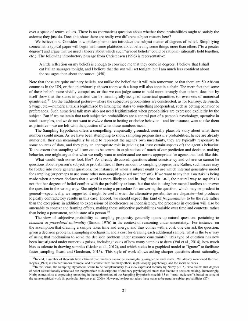
over a space of return values. There is no (normative) question about whether these probabilities ought to satisfy theaxioms; they just do. Does this show there are really two different subject matters here?

We believe not. Consider how philosophers often introduce the subject matter of degrees of belief. Simplifyingsomewhat, a typical paper will begin with some platitudes about believing some things more than others (“to a greaterdegree”) and argue that we need a theory about which such “graded beliefs” could be rational (rationally held together,etc.). The following introductory passage from Christensen (1996) is representative:

A little reflection on my beliefs is enough to convince me that they come in degrees. I believe that I shalleat Italian sausages tonight, and I believe that the sun will set tonight, but I am much less confident aboutthe sausages than about the sunset. (450)

Note that these are quite ordinary beliefs, not unlike the belief that it will rain tomorrow, or that there are 50 Africancountries in the UN, or that an arbitrarily chosen room with a lamp will also contain a chair. The mere fact that someof these beliefs more vividly compel us, or that we can judge some to hold more strongly than others, does not byitself show that the states in question can be meaningfully assigned numerical quantities (or even sets of numericalquantities).35 On the traditional picture—where the subjective probabilities are constructed, as for Ramsey, de Finetti,Savage, etc.—numerical talk is legitimized by linking the states to something independent, such as betting behavior orpreferences. Such numerical talk may also not need legitimization when probabilities are expressed explicitly by thesubject. But if we maintain that tacit subjective probabilities are a central part of a person’s psychology, operative instock examples, and we do not want to reduce them to betting or choice behavior—and for instance, want to take themas primitive—we are left with the question of what these numbers mean.

The Sampling Hypothesis offers a compelling, empirically grounded, neurally plausible story about what thesenumbers could mean. As we have been attempting to show, sampling propensities are probabilities, hence are alreadynumerical, they can meaningfully be said to represent the agent’s own uncertainty, they are typically responsive tosome sources of data, and they play an appropriate role in guiding (at least certain aspects of) the agent’s behavior.To the extent that sampling will turn out to be central in explanations of much of our prediction and decision-makingbehavior, one might argue that what we really want to understand are norms appropriate for agents that look like this.

What would such norms look like? As already discussed, questions about consistency and coherence cannot bequestions about a person’s subjective probabilities, if those amount to sampling propensities. Rather, such issues maybe folded into more general questions, for instance, of when a subject ought to use which internal generative modelfor sampling (or perhaps to use some other non-sampling-based mechanism). If we want to say that a mistake is beingmade when a person declares that a word is more likely to end in ‘ing’ than in ‘-n-’, the natural way to say this isnot that her degrees of belief conflict with the probability axioms, but that she is using her mental toolbox to answerthe question in the wrong way. She might be using a procedure for answering the question, which may be prudent ingeneral—specifically, we suggested it might be useful when the alternative possibilities are disparate—but produceslogically contradictory results in this case. Indeed, we should expect this kind of fragmentation to be the rule ratherthan the exception: in addition to expressions of incoherence or inconsistency, the processes in question will also beamenable to context and framing effects, making these subjective probabilities variable over time and contexts, ratherthan being a permanent, stable state of a person.36

The view of subjective probability as sampling propensity generally opens up natural questions pertaining tobounded or procedural rationality (Simon, 1976) in the context of reasoning under uncertainty. For instance, onthe assumption that drawing a sample takes time and energy, and thus comes with a cost, one can ask the question:given a decision problem, a sampling mechanism, and a cost for drawing each additional sample, what is the best wayof using that mechanism to solve the decision problem under resource constraints? This type of question has nowbeen investigated under numerous guises, including issues of how many samples to draw (Vul et al., 2014), how muchbias to tolerate in drawing samples (Lieder et al., 2012), and which nodes in a graphical model to “ignore” to facilitatefaster sampling (Icard and Goodman, 2015). This style of work allows asking sharper questions about rationality,

35Indeed, a number of theorists have claimed that numbers cannot be meaningfully assigned to such states. We already mentioned Harman.Keynes (1921) is another famous example, and of course there are many others, in philosophy, psychology, and the social sciences.

36In this sense, the Sampling Hypothesis seems to be complementary to a view expressed recently by Norby (2015), who claims that degreesof belief as traditionally conceived are inappropriate as descriptions of ordinary psychological states that feature in decision making. Interestingly,Norby comes close to expressing something in the neighborhood of the Sampling Hypothesis (see his §3 on “proto-credences”), based on some ofthe same empirical work (in particular Stewart et al. 2006). However, he does not takes these states to be genuine subject probabilities (87).

21

taking resource limitations into account, which also has the potential virtue of coming closer to concrete questionsabout how beings like us, who certainly share such limitations, ought to think and behave.37 In the other direction,it has been suggested that such (bounded) rationality considerations might play an important methodological role inhypothesis formation about how various cognitive mechanisms work (Griffiths et al., 2015; Icard, 2014), echoingearlier suggestions by both philosophers and psychologists (Dennett, 1981; Anderson, 1990).

To repeat once again, this is not to deny that there are other kinds of normative questions one can ask, e.g., thatmight apply to betting odds or other species of subjective probability. However, rather than casting doubt on whethersampling propensities ought to be considered bona fide subjective probabilities, we ought to see these new issues asimportant reflections of the fact that, however probabilities are represented in the mind (to the extent that they are),they must be represented in some format, and thus will inevitably require computational resources to use effectively.The Sampling Hypothesis provides a concrete proposal concerning that format, and thus presents a chance for askingnovel and precise questions about rationality in the context of probabilistic inference and reasoning.

13 ConclusionAccording to the Sampling Hypothesis, much of what we pre-theoretically think of as graded belief, and much of whatgoes under the heading of subjective probability in theorizing about human agency and intelligence, is represented inthe brain as a kind of sampling propensity of an internal generative model. In this way an important variety ofsubjective probability is reduced to a kind of objective probability, assumed to be operative in our thought and decisionmaking via a choice mechanism like DECISION RULE A or B. We have tried to present the view as clearly as possible,both at a conceptual level and at an empirical level, offering the most compelling evidence in its favor, and to showthat the view overcomes many of the common challenges to the idea that the mind does in fact use probabilities.

The Sampling Hypothesis ties together a number of otherwise disparate ideas and traditions within cognitive sci-ence into a single view: probabilistic models of learning and reasoning, connectionist models, the stochastic nature ofchoice and behavior, heuristics and biases, multistability in perception, probability matching, and bounded rationality.We also identified a number of conceptual and empirical challenges for the hypothesis. Given the nascent but promis-ing empirical support for the hypothesis, and its potential for clarifying the nature of philosophically important mentalstates and processes, raising new normative questions in addition, we believe the Sampling Hypothesis merits furtherattention, experimental investigation, and systematization.

ReferencesAnderson, J. R. (1990). The Adaptive Character of Thought. Lawrence Earlbaum Associates, Inc.

Anscombe, F. J. and Aumann, R. J. (1963). A definition of subjective probability. The Annals of MathematicalStatistics, 34(1):199–205.

Arora, S. and Barak, B. (2009). Computational Complexity: A Modern Approach. Cambridge University Press.

Barsalou, L. W. (1999). Perceptual symbol systems. Behavioral and Brain Sciences, 22(4):577–609.

Berkes, P., Orban, G., Lengyel, M., and Fiser, J. (2011). Spontaneous cortical activity reveals hallmarks of an optimalinternal model of the environment. Science, 331:83–87.

Buesing, L., Bill, J., Nessler, B., and Maass, W. (2011). Neural dynamics as sampling: A model for stochasticcomputation in recurrent networks of spiking neurons. PLoS Computational Biology, 7(11).

Carnap, R. (1947). On the application of inductive logic. Philosophy and Phenomenological Research, 8:133–148.

Chater, N. and Manning, C. D. (2006). Probabilistic models of language processing and acquisition. Trends inCognitive Science, 10(7):335–344.

37As mentioned above (§9), it has been common in this literature to rationalize behavior at odds with logic or probability by invoking notions ofboundedness or resource constraints.

22

Chater, N., Tenenbaum, J. B., and Yuille, A. (2006). Probabilistic models of cognition: Conceptual foundations.Trends in Cognitive Science, 10(7):287–291.

Christensen, D. (1996). Dutch-book arguments depragmatized: Epistemic consistency for partial believers. Journalof Philosophy, 93:450–479.

Churchland, P. S. and Sejnowski, T. J. (1994). The Computational Brain. MIT Press.

Clark, A. (2013). Whatever next? Predictive brains, situated agents, and the future of cognitive science. Behavioraland Brain Sciences, 36:181–253.

Craik, K. (1943). The Nature of Explanation. Cambridge University Press.

Davidson, D. (1975). Hempel on explaining action. Erkenntnis, 10(3):239–253.

Denison, S., Bonawitz, E., Gopnik, A., and Griffiths, T. L. (2013). Rational variability in children’s causal inferences:The Sampling Hypothesis. Cognition, 126:285–300.

Dennett, D. C. (1981). Three kinds of intentional psychology. In Healey, R., editor, Reduction, Time, and Reality,pages 37–61. Cambridge University Press.

Dreyfus, H. L. and Dreyfus, S. E. (1986). Mind over Machine. Free Press.

Eriksson, L. and Hajek, A. (2007). What are degrees of belief? Studia Logica, 86(2):183–213.

de Finetti, B. (1974). Theory of Probability, volume 1. Wiley, New York.

Fiser, J., Berkes, P., Orban, G., and Lengyel, M. (2010). Statistically optimal perception and learning: from behaviorto neural representations. Trends in Cognitive Science, 14(3):119–130.

Freer, C., Roy, D., and Tenenbaum, J. (2012). Towards common-sense reasoning via conditional simulation: Legaciesof Turing in artificial intelligence. In Downey, R., editor, Turing’s Legacy. ASL Lecture Notes in Logic.

Gaifman, H. (2004). Reasoning with limited resources and assigning probabilities to arithmetical statements. Synthese,140:97–119.

Galton, F. (1889). Natural Inheritance. MacMillan.

Gendler, T. (2008). Alief and belief. Journal of Philosophy, 105(10):634–663.

Gershman, S. J. and Daw, N. D. (2012). Perception, action, and utility: the tangled skein. In Rabinovich, M., Friston,K., and Varona, P., editors, Principles of Brain Dynamics: Global State Interactions, pages 293–312. MIT Press.

Gershman, S. J., Vul, E., and Tenenbaum, J. B. (2012). Multistability and perceptual inference. Neural Computation,24:1–24.

Gigerenzer, G. and Goldstein, D. G. (1996). Reasoning the fast and frugal way: Models of bounded rationality.Psychological Review, 103(4):650–699.

Good, I. J. (1950). Probability and the Weighing of Evidence. Charles Griffin.

Good, I. J. (1983). Good Thinking: The Foundations of Probability and Its Applications. University of MinnesotaPress.

Goodman, N. D., Tenenbaum, J. B., and Gerstenberg, T. (2014). Concepts in a probabilistic language of thought. InMargolis, E. and Laurence, S., editors, The Conceptual Mind: New Directions in the Study of Concepts. MIT Press.

Gopnik, A., Glymour, C., Sobel, D., Schulz, L., Kushnir, T., and Danks, D. (2004). A theory of causal learning inchildren: Causal maps and Bayes nets. Psychological Review, 111(1):3–32.

23

Griffiths, T. L., Chater, N., Kemp, C., Perfors, A., and Tenenbaum, J. B. (2010). Probabilistic models of cognition:exploring representations and inductive biases. Trends in Cognitive Science, 14(8):357–364.

Griffiths, T. L., Lieder, F., and Goodman, N. D. (2015). Rational use of cognitive resources: Levels of analysis betweenthe computational and the algorithmic. Topics in Cognitive Science, 7(2):217–229.

Griffiths, T. L. and Tenenbaum, J. B. (2006). Optimal predictions in everyday cognition. Psychological Science,17(9):767–773.

Harman, G. (1986). Change in View. MIT Press.

Icard, T. (2013). The Algorithmic Mind: A Study of Inference in Action. PhD thesis, Stanford University.

Icard, T. F. (2014). Toward boundedly rational analysis. In Bello, P., Guarini, M., McShane, M., and Scassellati, B.,editors, Proceedings of the 36th Annual Meeting of the Cognitive Science Society, pages 637–642.

Icard, T. F. and Goodman, N. D. (2015). A resource-rational approach to the causal frame problem. In Noelle, D. C.,Dale, R., Warlaumont, A. S., Yoshimi, J., Matlock, T., Jennings, C. D., and Maglio, P. P., editors, Proceedings ofthe 37th Annual Conference of the Cognitive Science Society.

James, W. (1890). The Principles of Psychology. Henry Holt & Co.

Jaynes, E. T. (2003). Probability Theory: The Logic of Science. Cambridge University Press.

Johnson-Laird, P. N. (1983). Mental Models: Towards a Cognitive Science of Language, Inference, and Consciousness.Cambridge University Press.

Joyce, J. M. (1998). A nonpragmatic vindication of probabilism. Philosophy of Science, 65:575–603.

Keynes, J. M. (1921). A Treatise on Probability. Macmillan.

Knill, D. C. and Pouget, A. (2004). The Bayesian brain: the role of uncertainty in neural coding and computation.Trends in Neurosciences, 27(12):712–719.

Koller, D. and Friedman, N. (2009). Probabilistic Graphical Models: Principles and Techniques. MIT Press.

Kruschke, J. K. (2006). Locally Bayesian learning with application to retrospective revaluation and highlighting.Psychological Review, 113(4):677–699.

Kwisthout, J., Wareham, T., and van Rooij, I. (2008). Bayesian intractability is not an ailment that approximation cancure. Cognitive Science, 35:779–784.

Lee, T. S. and Mumford, D. (2003). Hierarchical bayesian inference in the visual cortex. Journal of the Optical Societyof America, A, 20(7):1434–1448.

Levy, R., Reali, F., and Griffiths, T. L. (2009). Modeling the effects of memory on human online sentence processingwith particle filters. Advances in Neural Information Processing Systems, 21:937–944.

Lewis, D. K. (1974). Radical interpretation. Synthese, 23:331–344.

Lichtenstein, S., Slovic, P., Fischoff, B., Layman, M., and Combs, B. (1978). Judged frequency of lethal events.Journal of Experimental Psychology: Human Learning and Memory, 4(6).

Lieder, F., Griffiths, T. L., and Goodman, N. D. (2012). Burn-in, bias, and the rationality of anchoring. Advances inNeural Information Processing Systems, 25:2699–2707.

Lieder, F., Hsu, M., and Griffiths, T. L. (2014). The high availability of extreme events serves resource-rationaldecision-making. In Bello, P., Guarini, M., McShane, M., and Scassellati, B., editors, Proceedings of the 36thAnnual Meeting in Cognitive Science.

24

Lochmann, T. and Deneve, S. (2011). Neural processing as causal inference. Current Opinion in Neurobiology,21:774–781.

Luce, R. D. (1959). Individual Choice Behavior: A Theoretical Analysis. John Wiley & Sons.

Luce, R. D. and Suppes, P. (1965). Preference, utility, and subjective probability. In Luce, R. D., Bush, R. R., andGalanter, E. H., editors, Handbook of Mathematical Psychology, volume 3, pages 249–410. Wiley.

MacKay, D. (2003). Information Theory, Inference, and Learning Algorithms. Cambridge University Press.

Mandelbaum, E. (2014). Thinking is believing. Inquiry: An Interdisciplinary Journal of Philosophy, 57(1):55–96.

Marr, D. (1982). Vision. W.H. Freeman and Company.

McFadden, D. L. (1973). Conditional logit analysis of qualitative choice behavior. In Zarembka, P., editor, Frontiersin Econometrics. Academic Press.

Millgram, E. (1991). Harman’s hardness arguments. Pacific Philosophical Quarterly, 72(3):181–202.

Moreno-Bote, R., Knill, D. C., and Pouget, A. (2011). Bayesian sampling in visual perception. Proceedings of theNational Academy of Sciences, 108(30):12491–12496.

Mozer, M. C., Pashler, H., and Homaei, H. (2008). Optimal predictions in everyday cognition: The wisdom ofindividuals or crowds? Cognitive Science, 32:1133–1147.

Norby, A. (2015). Uncertainty without all the doubt. Mind and Language, 30(1):70–94.

Pearl, J. (1988). Probabilistic Reasoning in Intelligent Systems: Networks of Plausible Inference. Morgan Kaufmann.

Perfors, A. (2012). Bayesian models of cognition: What’s built in after all? Philosophy Compass, 7(2):127–138.

Raiffa, H. (1968). Decision Analysis. Addison-Wesley.

Ramsey, F. P. (1931). Truth and probability. In Braithwaite, R. B., editor, Foundations of Mathematics and OtherLogical Essays. Martino Fine.

Rosch, E. (1975). Cognitive representations of semantic categories. Journal of Experimental Psychology: General,104(3):192–233.

Rumelhart, D. E., McClelland, J. L., and The PDP Research Group (1986). Parallel Distributed Processing: Explo-rations in the Microstructure of Cognition. MIT Press.

Savage, L. J. (1954). The Foundations of Statistics. John Wiley and Sons.

Schacter, D. L., Addis, D. R., and Buckner, R. L. (2008). Episodic simulation of future events: Concepts, data, andapplications. Annals of the New York Academy of Sciences, 1124:39–60.

Schwarz, N., Bless, H., Strack, F., Klumpp, G., Rittenauer-Schatka, H., and Simons, A. (1991). Ease of retrieval asinformation: Another look at the availability heuristic. Journal of Personality and Social Psychology, 61(2):195–202.

Seth, A. K. (1999). Evolving behavioural choice: An exploration of Hernnstein’s Matching Law. In Floreano, D.,Nicoud, J.-D., and Mondada, F., editors, Proceedings of the Fifth European Conference on Artificial Life, pages225–236. Springer.

Shi, L., Griffiths, T. L., Feldman, N. H., and Sanborn, A. N. (2010). Exemplar models as a mechanism for performingBayesian inference. Psychonomic Bulletin and Review, 17(4):443–464.

Simon, H. A. (1976). From substantive to procedural rationality. In Kastelein, T. J., Kuipers, S. K., Nijenhuis, W. A.,and Wagenaar, G. R., editors, 25 Years of Economic Theory, pages 65–86. Springer.

25

Solway, A. and Botvinick, M. M. (2012). Goal-directed decision making as probabilistic inference. PsychologicalReview, 119(1):120–154.

Stewart, N., Chater, N., and Brown, G. D. (2006). Decision by sampling. Cognitive Psychology, 53:1–26.

Sundareswara, R. and Schrater, P. (2007). Perceptual multistability predicted by search model for Bayesian decisions.Journal of Vision, 8(5):1–19.

Suppes, P. (1974). The measurement of belief. The Journal of the Royal Statistical Society, Series B, 36(2):160–191.

Tenenbaum, J. T., Kemp, C., Griffiths, T. L., and Goodman, N. D. (2011). How to grow a mind: Statistics, structure,and abstraction. Science, 331:1279–1285.

Thurstone, L. L. (1927). A law of comparative judgment. Psychological Review, 34(4):273–286.

Tversky, A. and Kahneman, D. (1974). Judgment under uncertainty: Heuristics and biases. Science, 185(4157):1124–1131.

Tversky, A. and Kahneman, D. (1983). Extensional versus intuitive reasoning: The conjunction fallacy in probabilityjudgment. Psychological Review, 90(4):293–315.

Vilares, I. and Kording, K. P. (2011). Bayesian models: the structure of the world, uncertainty, behavior, and the brain.Annals of the New York Academy of Sciences, 1224:22–39.

Vul, E. (2010). Sampling in Human Cognition. PhD thesis, MIT.

Vul, E., Goodman, N. D., Griffiths, T. L., and Tenenbaum, J. B. (2014). One and done? Optimal decisions from veryfew samples. Cognitive Science, 38(4):599–637.

Vul, E. and Pashler, H. (2008). Measuring the crowd within. Psychological Science, 19(7):645–647.

Vulcan, N. (2000). An economist’s perspective on probability matching. Journal of Economic Surveys, 13(1):101–118.

Walley, P. (1991). Statistical Reasoning with Imprecise Probabilities. Chapman & Hall.

Williamson, T. (2015). Acting on knowledge. In Carter, J. A., Gordon, E., and Jarvis, B., editors, Knowledge-First.Oxford University Press.

Yang, T. and Shadlen, M. N. (2007). Probabilistic reasoning by neurons. Nature, 447:1075–1082.

Yurovsky, D., Boyer, T. W., Smith, L. B., and Yu, C. (2013). Probabilistic cue combination: Less is more. Develop-mental Science, 16(2):149–158.

Zynda, L. (2000). Representation theorems and realism about degrees of belief. Philosophy of Science, 67(1):45–69.

A Boltzmann Machine as Gibbs SamplerIn this Appendix we explain the sense in which the activation rule for the Boltzmann Machine carries out Gibbssampling on an underlying Markov random field. This fact is folklore in cognitive science.

Gibbs sampling is an instance of the Metropolis-Hastings algorithm, which in turn is a typle of Markov chainMonte Carlo inference (MacKay, 2003). Suppose we have a multivariate distribution P(X1, . . . ,Xn) and we want todraw samples from it. The Gibbs sampling algorithm is as follows:

1. Specify some initial values for all the random variables y(0) = (y(0)1 , . . . ,y(0)n ).

2. Given y(r), randomly choose a number i ∈ {0, . . . ,n}, and let y(r+1) be exactly like y(r), except that y(r+1)i is

redrawn from the conditional distribution P(Xi | y−i).

26

3. At some stage R, return some subset of {y(0), . . . ,y(R)} as samples.

Note that the sequence of value vectors y(0), . . . ,y(r), . . . forms a Markov chain because the next sample y(r+1) onlydepends on the previous sample y(r). Let q(y→ y′) be the probability of moving from y at a given stage r to y′ at stager+1 (which is the same for all r, and equal to 0 when y and y′ differ by more than one coordinate.). And let πr(y) bethe probability of being in state y at stage r. Then we clearly have:

πr+1(y′) = ∑

yπ

r(y)q(y→ y′) .

By general facts about Markov chains, it can be shown that this process reaches a unique stationary distribution, i.e.,πr = πr+1 for all r > s for some s. This is the unique distribution π∗ for which the following holds:

π∗(y′) = ∑

yπ∗(y)q(y→ y′) .

Since this equation also holds for P, that shows the Markov chain converges to P = π∗.Recall the Boltzmann Machine is defined by a set of nodes and weights between those nodes.38 If we think of the

nodes as binary random variables (X1, . . . ,Xn), taking on values {0,1}, then the weight matrix W gives us a naturaldistribution P(X1, . . . ,Xn) on state space {0,1}n as follows. First, define an energy function E on the state space:

E(y) =−12 ∑

i, jWi, jyiy j .

Then the resulting Boltzmann distribution is given by:

P(y) =e−E(y)

∑y′ e−E(y′) .

Note that the denominator becomes a very large sum very quickly. Recall from our earlier discussion that the size ofthe state space is 32 with 5 nodes, but over a trillion with 40 nodes. Suppose we apply the Gibbs sampling algorithmto this distribution. Then at a given stage, we randomly choose a node to update, and the new value is determinedby the conditional probability as above. This step is equivalent to applying the activation function for the BoltzmannMachine (where in the following, y′ is just like y, except that y′i = 1 and yi = 0):

P(Xi = 1 | {y j} j 6=i) = P(Xi = 1 | y or y′)

=P(y′)

P(y or y′)

=e−E(y′)

e−E(y)+ e−E(y′)

=1

1+ eE(y′)−E(y)

=1

1+ e−∑ j Wi, jy j

=1

1+ e−neti.

Thus, the above argument shows that the Boltzmann Machine (eventually) samples from the associated Boltzmanndistribution. Incidentally, we can also see now why neti is equivalent to the log odds ratio under the Boltzmann

38We ignore bias terms here to simplify the presentation. See Rumelhart et al. (1986) for the general formulation.

27

distribution (recall the discussion in §8 of the Yang and Shadlen 2007 experiment):

P(y′)P(y)

=e−E(y′)

e−E(y)

= eE(y)−E(y′)

= e∑ j Wi, jy j

= eneti .

And thus,

logP(y′)P(y)

= log(eneti

)= neti .

B Softmax versus Sampling RuleIn this Appendix, we offer some observations about the relation between the softmax (or generalized Luce-Shepard)choice rule and the sampling-based decision rules discussed in this chapter. Suppose we associate with a subject aprobability function P(·) on sample space H = {H1, . . . ,Hn} and a utility u over actions A = {A1, . . . ,Am}.

The softmax rule says that the subject will give response A with probability

ev(A)/β

∑A′∈A ev(A′)/β,

where v is some value function, which in this case we will assume is the log expected utility:

v(H) = log ∑H∈H

P(H)u(A,H).

As a representative example of a sampling based rule, recall DECISION RULE B:

DECISION RULE B: Suppose we are given a generative model M with V as possible return values. Toselect an action, take R samples, H(1), . . . ,H(R), using M , and let BEST be the set of actions that receivethe largest summed utilities, i.e.,

BEST = {A j :R

∑i=1

u(A j,H(i)) is maximal}.

Take action A j ∈ BEST with probability 1|BEST| .

In the specific case of a certain kind of estimation problem—where H = A and the utility of an estimate is 1 if correct,0 otherwise; thus expected utility and probability coincide—it is easy to see that the softmax rule with β = 1 andDECISION RULE B with R = 1 (or R = 2) are equivalent. The probability of returning hypothesis H is just P(H), i.e.,we have probability matching.

Unfortunately, even restricting to these simple estimation problems, the relation between the two rules as functionsof β and R is intractable and varies with the probability distribution P(·), as Vul (2010) points out. Thus, beyond β =R = 1 it is hard to study their relationship. As mentioned in the text, both can be used to fit much of the psychologicaldata, though one might suspect the sampling rule is more reasonable on the basis of computational considerations.

Interestingly, for more general classes of decision problems, these two classes of rules can be qualitatively distin-guished. The Luce Choice Axiom, from which the Luce choice rule was originally derived (Luce, 1959), gives a hintof how we might do this. Where PS(T ) is the probability of choosing an action from T ⊆ A from among options inS⊆ A , the choice axiom states that for all R such that T ⊆ R⊆ S:

PS(T ) = PS(R) PR(T ) .

28

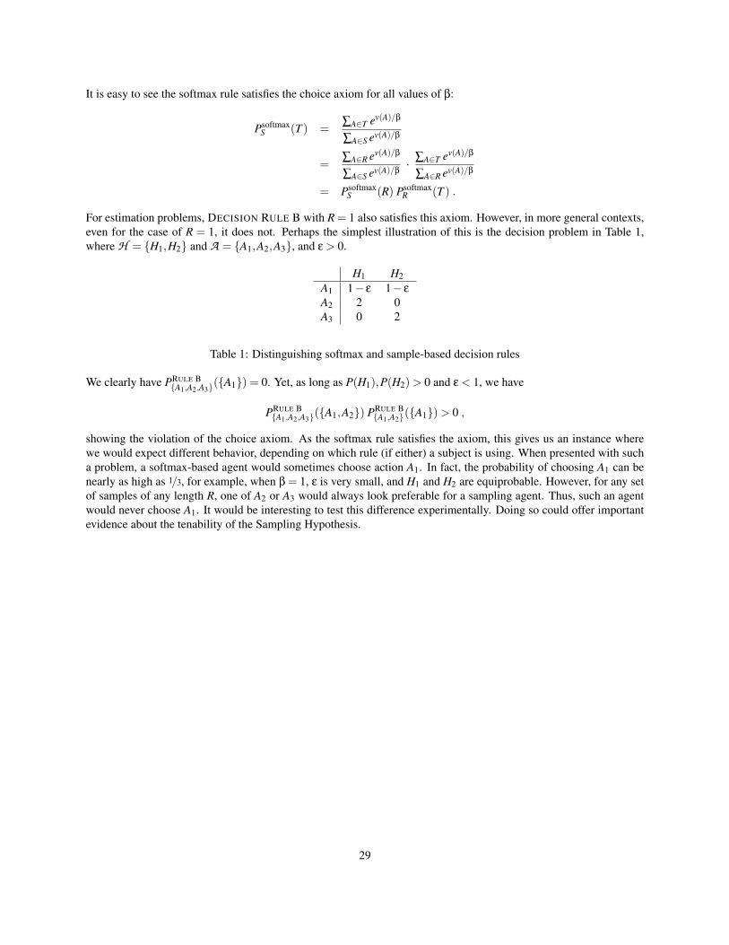
It is easy to see the softmax rule satisfies the choice axiom for all values of β:

PsoftmaxS (T ) =

∑A∈T ev(A)/β

∑A∈S ev(A)/β

=∑A∈R ev(A)/β

∑A∈S ev(A)/β· ∑A∈T ev(A)/β

∑A∈R ev(A)/β

= PsoftmaxS (R) Psoftmax

R (T ) .

For estimation problems, DECISION RULE B with R = 1 also satisfies this axiom. However, in more general contexts,even for the case of R = 1, it does not. Perhaps the simplest illustration of this is the decision problem in Table 1,where H = {H1,H2} and A = {A1,A2,A3}, and ε > 0.

H1 H2A1 1− ε 1− ε

A2 2 0A3 0 2

Table 1: Distinguishing softmax and sample-based decision rules

We clearly have PRULE B{A1,A2,A3}({A1}) = 0. Yet, as long as P(H1),P(H2)> 0 and ε < 1, we have

PRULE B{A1,A2,A3}({A1,A2}) PRULE B

{A1,A2}({A1})> 0 ,

showing the violation of the choice axiom. As the softmax rule satisfies the axiom, this gives us an instance wherewe would expect different behavior, depending on which rule (if either) a subject is using. When presented with sucha problem, a softmax-based agent would sometimes choose action A1. In fact, the probability of choosing A1 can benearly as high as 1/3, for example, when β = 1, ε is very small, and H1 and H2 are equiprobable. However, for any setof samples of any length R, one of A2 or A3 would always look preferable for a sampling agent. Thus, such an agentwould never choose A1. It would be interesting to test this difference experimentally. Doing so could offer importantevidence about the tenability of the Sampling Hypothesis.

29