This paper presents preliminary findings and is being distributed to economists

and other interested readers solely to stimulate discussion and elicit comments.

The views expressed in this paper are those of the authors and do not necessarily

reflect the position of the Federal Reserve Bank of New York or the Federal

Reserve System. Any errors or omissions are the responsibility of the authors.

Federal Reserve Bank of New York

Staff Reports

Subjective Intertemporal Substitution

Richard K. Crump

Stefano Eusepi

Andrea Tambalotti

Giorgio Topa

Staff Report No. 734

July 2015

Revised July 2020

Subjective Intertemporal Substitution

Richard K. Crump, Stefano Eusepi, Andrea Tambalotti, and Giorgio Topa

Federal Reserve Bank of New York Staff Reports, no. 734

July 2015; revised July 2020

JEL classification: D12, D15, D84, E21

Abstract

We estimate the elasticity of intertemporal substitution (EIS)—the response of expected

consumption growth to changes in the real interest rate—using subjective expectations data from

the New York Fed’s Survey of Consumer Expectations (SCE). This unique data set allows us to

estimate the consumption Euler equation with no auxiliary assumptions on the properties of

expectations, which are instead necessary when using choice data. We find a subjective EIS of

about 0.5, consistent with the results of much of the literature. In addition, planned consumption

displays excess sensitivity to expected income changes, even among households not facing

substantial liquidity constraints.

Key words: subjective expectations, inflation expectations, Euler equation, elasticity of

intertemporal substitution

_________________

Crump, Tambalotti, Topa: Federal Reserve Bank of New York (emails: richard.crump@ny.frb.org, andrea.tambalotti@ny.frb.org, giorgio.topa@ny.frb.org). Eusepi: University of Texas at Austin (email: stefano.eusepi@austin.utexas.edu). The authors would like to thank Manuel Arellano, Adrien Auclert, Mark Bils, Stéphane Bonhomme, Chris Carroll, Keshav Dogra, Andrea Ferrero, Andreas Fuster, Giacomo De Giorgi, Simon Gilchrist, Sydney Ludvigson, Alexander Michaelides, Giuseppe Moscarini, Jonathan Parker, Ben Pugsley, Ricardo Perez-Truglia, Giorgio Primiceri, Ricardo Reis, Gianluca Violante, our discussants Dario Caldara, Monica Paiella, and Eric Sims, as well as seminar and conference participants for helpful comments and suggestions. Zachary Bleemer, Matthew Yeaton, Nima Dahir, and Jiwon Lee provided excellent research assistance. The views expressed in this paper are those of the authors and do not necessarily represent the position of the Federal Reserve Bank of New York or the Federal Reserve System. To view the authors’ disclosure statements, visit https://www.newyorkfed.org/research/staff_reports/sr734.html.

1 Introduction

Intertemporal substitution, the response of planned consumption growth to changes in theexpected rate of return, is at the heart of virtually every modern dynamic model in bothmacroeconomics and finance. Starting from the pioneering work of Hall (1978, 1988) andHansen and Singleton (1982, 1983), a large literature has endeavored to quantify this mecha-nism. However, a clear consensus on the magnitude of the key parameter that governs it—theelasticity of intertemporal substitution (EIS)—remains elusive. For example, a recent metastudy by Havranek (2015) based on 2,735 estimates from 169 published papers reports adistribution of estimates that ranges from -5 to 5, with clusters near both 0 and 1. The EISis difficult to pin down in part because measuring expected consumption growth and rates ofreturn, as envisioned in the theory, is challenging. Much of the empirical literature proceedsby replacing expectations with realizations, which together with auxiliary assumptions onthe resulting forecast errors, allows the estimation of the consumption Euler equation andits slope with the generalized method of moments (GMM).

In this paper, we bypass this challenge entirely by estimating the Euler equation withdirect measures of households’ subjective expectations of both consumption growth and in-flation. The latter provide variation in the perceived real interest rate. This approach doesnot rely on auxiliary assumptions on the process that generates the expectations. Not havingto take a stand on expectation formation is especially valuable because a growing body ofevidence has documented many deviations from the simple rational benchmark, but it hasnot yet resulted in a widely accepted alternative modeling paradigm.

This straightforward yet original empirical strategy is made possible by the unique datacollected in the Federal Reserve Bank of New York’s Survey of Consumer Expectations(SCE). Unlike other available sources of information on expectations, this nationally repre-sentative monthly survey asks a rotating panel of approximately 1,300 U.S. household headsa series of quantitative questions on spending plans and future inflation, as well as on manyother macroeconomic developments and household choices and experiences. Some of thesequestions elicit subjective probabilities of future outcomes, while others focus on point ex-pectations. From the survey responses, we can derive clean measures of the moments ofthe subjective distributions of spending growth and inflation that are suitable for estimatingconsumption Euler equations at the household level with little or no manipulation of the rawdata.1

1As a comparison, the Michigan Survey of Consumers provides quantitative information on inflationexpectations, but only qualitative measures of households’ readiness to spend on durable goods. Thesemeasures can proxy for current consumption, but they cannot be used to infer planned future consumptiongrowth, as discussed for instance by Bachmann, Berg, and Sims (2015).

1

The starting point for our empirical analysis is a first order approximation of the mostbasic consumption Euler equation, which relates expected consumption growth to the realinterest rate, while excluding all other variables. This relationship is the first order conditionof an intertemporal consumption choice problem, under familiar assumptions on the formof consumers’ utility and constraints. In this framework, the EIS represents a structuralparameter pertaining to the underlying optimization problem, rather than a measure of thecausal effect of inflation expectations on consumption, or its growth rate, or its expectation,as in many studies based on expectations data (e.g., D’Acunto, Hoang, and Weber (2018)).

Thanks to the wealth of household level data collected by the SCE, we can also exploremuch more general specifications of the Euler equation. Underlying all these specificationsis a consumption choice problem of the same type described above, but whose objective orconstraints are different, and usually more complex, than those posited in the baseline case.Nevertheless, the same empirical approach described above applies to these more complexequations as well. We allow for non separability between consumption and leisure, nonisoelastic preferences, life-cycle effects proxied by demographic variables, and the presenceof financial constraints. These extensions cover most of the alternatives that have beenexamined in the literature. Furthermore, we take advantage of the probabilistic nature ofsome of the SCE questions to address misspecification concerns that are hard to avoid withexisting data. We consider specifications which include the second moments of the reportedprobability distributions of the relevant variables to account for possible failures of the firstorder approximation of the Euler equation. Controlling for these higher moments is especiallyuseful when trying to distinguish among alternative sources of excess sensitivity of plannedconsumption to expected income growth (e.g., Carroll 2001).

The estimated EIS in the basic specification is between 0.7 and 0.8, at the upper end of therange of microeconomic estimates based on choice data, as surveyed for instance in Attanasio(1999) and Attanasio and Weber (2010). This estimate is strongly statistically significantand is robust to the inclusion of a large set of controls in the regression, which accountfor many possible extensions of the simplest Euler equation. When we include expectedincome growth among these controls, however, we uncover statistically strong and consistentevidence of a response of planned consumption to predictable income changes. This so-called excess sensitivity survives even after controlling for many of the potential confoundingfactors that have been considered in the literature, such as preference non separabilities andliquidity constraints. To account for the latter, we split the sample to focus on householdsthat are unlikely to be financially constrained. We do so based on a range of criteria, someof which depend on the answers to questions that are unique to the SCE and that addressthe respondents’ financial health directly. Even among these households, the evidence in

2

favor of excess sensitivity is statistically significant, and only marginally less strong thanfor those who are more likely to be constrained. This result is consistent with a growingbody of evidence of excess income sensitivity and anomalously high marginal propensitiesto consume among rich households with high liquid wealth (e.g. Parker 2017, Kueng 2018,Fagereng, Holm, and Natvik 2018.)

Once we control for the presence of excess sensitivity, the estimates of the EIS are closerto 0.5. This value is toward the lower end of the range of micro estimates reported inthe literature, but a bit above the corrected mean reported in the meta study by Havranek(2015). In the sample of papers that he considers, the mean of the estimates for asset holdersis around 0.3-0.4, once corrected for the selective reporting bias associated with discardingnegative and insignificant estimates too often. A value of 0.5 is also consistent with standardcalibrations in macroeconomic studies (e.g., Hall 2009, 2016), although not with the commonassumption of logarithmic utility in consumption.

Overall, we come away from this study with a sharper view of the plausible values ofthe EIS compared to that entertained by the existing literature. Even if our estimatesrange roughly between 0.5 and 0.8, they are statistically very precise conditional on anygiven specification of the Euler equation. And even this range of variation across models issmall compared to what is common within studies based on choice data. One qualificationto these conclusions is that the strong evidence of excess sensitivity to expected incomegrowth that is present in our data might shed some doubts on the Euler equation frameworkon which the analysis is predicated, and hence on the interpretation of our estimates ascapturing a “structural” EIS. There are two possible answers to these doubts. The firstone is that expected income growth might in fact be significant in the regressions because itproxies for some other omitted or poorly measured factor that belongs in the Euler equation.One such factor might be perceived wealth, as in the model of Lian (2019). The secondpossibility is to step outside of the Euler equation framework entirely. Even in this case,however, the elasticity of expected consumption growth to expected inflation that we estimatemeasures a well defined (conditional) subjective elasticity. This coefficient is informativeabout households’ consumption plans and it can be a useful moment to discriminate amongalternative models of consumption, even if it is not “the” EIS. Developing models that areconsistent with all our findings, and in particular with the pervasive evidence of excess incomesensitivity even among unconstrained households, is beyond the scope of this paper.

The paper is organized as follows. The following subsection discusses the related literatureto this paper. Section 2 provides the theoretical motivations for our empirical specification.Details of the data set are in Section 3. Sections 4 and 5 provide our main results whilerobustness checks and additional results are reported in Section 6. Section 7 concludes and

3

discusses directions for further work.

1.1 Related Literature

This paper is most directly related to the vast empirical literature that estimates the EIS.Much of this work exploits the moment restrictions embedded in the consumption Eulerequation within a GMM framework to estimate preference parameters and to test the theoryusing either aggregate or, more often, microeconomic data. Attanasio (1999) and Attanasioand Weber (2010) are two recent surveys that put this literature in the broader contextof research on consumption. Browning and Lusardi (1996) is an earlier survey focusingon the first wave of this research based on micro data, including seminal contributions byHall and Mishkin (1982) and Zeldes (1989) using the Panel Study of Income Dynamics(PSID), Meghir and Weber (1996) and Attanasio and Weber (1995) using the ConsumerExpenditure Survey (CEX), and Attanasio and Weber (1993) using the Family ExpenditureSurvey (FES) in the UK. Many other empirical approaches and data sources have also beenemployed to estimate the EIS. For example, Barsky, Juster, Kimball, and Shapiro (1997) usesurvey responses to questions about specific hypothetical situations; Gruber (2013) exploitsindividual variation in capital income tax rates; Engelhardt and Kumar (2009) is based ondifferences in employer matching rates in 401(k) plans; Cashin and Unayama (2012) look atan increase in the consumption tax rate in Japan; and Best, Cloyne, Ilzetzki, and Kleven(2020) use mortgage notches in the UK. Alan and Browning (2010) use synthetic residualestimation as an alternative to GMM.

Few papers use expectations data in the context of estimating Euler equations. Jappelliand Pistaferri (2000) do so with data from the Bank of Italy Survey of Household Income andWealth, focusing on tests of excess sensitivity. They estimate a standard equation for realizedconsumption, but they use subjective income and inflation expectations as instruments topredict income growth. More recently, Christelis, Georgarakos, Jappelli, and van Rooij(2020) estimate the strength of the precautionary saving motive with data from the DutchCentER Internet panel.

Our reliance on expectations data also puts us in contact with the growing literature thatstudies the properties of the expectations of households, firms, and other agents to refineand test economic theories (e.g., Fuster, Kaplan, and Zafar 2020). A prominent strandof this literature focuses on the inflation expectations of households, firms, and professionalforecasters (e.g. Mankiw, Reis, and Wolfers 2003, Coibion and Gorodnichenko 2012, Andradeand Le Bihan 2013, Coibion, Gorodnichenko, and Kumar 2018, Coibion and Gorodnichenko2015, Fuhrer 2015, Malmendier and Nagel 2016, Andrade, Crump, Eusepi, and Moench 2016,

4

and Wiederholt and Vellekoop 2017). Beyond inflation, many papers study expectations ona wide variety of economic and financial variables. Some prominent examples are Souleles(2004), who looks at consumption and sentiment in the Michigan Survey; Greenwood andShleifer (2014) who study investor expectations of stock returns; and Gennaioli, Ma, andShleifer (2015) who investigate the relationship between investment and expectations ofearnings growth in a survey of CFOs. A common finding among many of these papers is thatexpectations do not appear to conform to the simple full-information, rational benchmark.This evidence supports our empirical approach which relies on observed expectations ratherthan on an explicit model of how they are formed.

At the intersection of these two literatures, several recent papers study the connectionbetween consumption and inflation expectations. Burke and Ozdagli (2013) use responsesto a series of survey modules appended to RAND’s American Life Panel to estimate therelationship between current realized consumption growth and inflation expectations.2 Simi-larly, Bachmann, Berg, and Sims (2015) estimate an ordered probit model of the relationshipbetween “readiness to spend” on durable goods and inflation expectations in the MichiganSurvey of Consumers. They also interpret the readiness to spend measure as a proxy forcurrent expenditures. Both these papers find little evidence of a connection between in-flation expectations and current consumption. On the contrary, D’Acunto, Hoang, andWeber (2018) and Ichiue and Nishiguchi (2015) find a stronger link in analogous Germanand Japanese survey data, respectively. The first study carefully exploits a difference-in-difference design to try and isolate the causal effect of changes in inflation expectations onspending and finds it to be large. The second study estimates the reaction of qualitativeproxies for both current and future planned spending to changes in inflation expectations.It finds the former to be negative and the latter to be positive, consistent with our results.

Due to data limitations, these studies cannot estimate the EIS, since doing so requiresdata on expected future consumption growth over the same horizon as inflation expecta-tions.3 Instead, these papers attempt to estimate an elasticity more akin to the partialderivative of the consumption function with respect to expected inflation. The challengewith this kind of exercise is that this partial derivative is a reduced form coefficient thatdepends on the details of the individual choice problem and of the macroeconomic environ-ment in which that choice takes place, as discussed by Hall (1988). This might explain why

2These survey modules were designed by a team of researchers from the New York Fed and variousacademic institutions. They served as a pilot for the SCE, as discussed in Bruine de Bruin, Manski, Topa,and van der Klaauw (2011).

3Among these studies, the regression that is closest to our specification is the one of future plannedspending on inflation expectations in Ichiue and Nishiguchi (2015). They still cannot recover an estimate ofthe EIS because their survey only provides directional information on planned spending.

5

studies based on different data in different periods tend to recover different values for thatcoefficient. To our knowledge, this is the first study to combine high quality survey data onboth consumption growth and inflation expectations to estimate an Euler equation, and inparticular the elasticity of intertemporal substitution.

2 Theoretical Framework

The theoretical underpinning of our estimation exercise is the standard intertemporal Eulerequation, which encapsulates the optimal consumption and saving choice of a householdthat can freely borrow and lend at a known (gross) nominal rate of return Rt. In its basicspecification with separable isoelastic preferences, this equilibrium condition can be writtenas

1 = Eit

[βi

(Ci

t+1

Cit

)− 1σ(

Rt

Πt+1

)], (2.1)

where βi is household’s i discount factor and Cit is its consumption of a bundle of goods and

services, including potentially those from durable goods. The overall level of this consump-tion can vary across i’s—we are not assuming the existence of a representative consumer—but the bundle’s composition and hence its relevant price index, denoted by Πt, does not.The assumption of a “representative” price index, whose rate of change defines aggregateconsumer inflation, is nearly universal in macroeconomics and it forms the basis of inflationmeasurement. It is also consistent with the SCE survey questions, which have been explicitlydeveloped to elicit expectations of aggregate inflation, rather than of the change in pricesthat might be more directly salient for the individual respondents as discussed in Section 3.

As suggested by the i superscript on the expectation operator, those expectations areallowed to be heterogeneous across households, as they are in our data. This heterogeneityin inflation expectations is a source of variation in the ex-ante real interest rate perceived bydifferent households over time, for any given level of the nominal interest rate. Accordingto the Euler equation, this variation should be associated with differences in planned con-sumption. Our estimates of the elasticity of intertemporal substitution, which is denoted byσ, measure the strength of this association.

We refer to these estimates as subjective measures of intertemporal substitution becausethey reflect the relationship between households’ subjective views of future inflation andconsumption growth. In this respect, these estimates are more directly related to individualEuler equations than those derived from observed consumption choices and rates of return,because the latter rely on specific assumptions on the properties of the expectations operatorto connect realizations back to the agents’ expectations featured in the equation. In contrast,

6

we do not need to take a stand on the nature of the expectation formation process, and inparticular on the sources of the observed heterogeneity in expectations, since we observethem directly.4

Taking a log-linear approximation of (2.1) yields the familiar relationship

Eit

[∆cit+1

]= σ log βi + σrt − σEi

t [πt+1] + oi,t, (2.2)

where lowercase letters represent logs and oi,t is a remainder collecting second and higherorder terms in the approximation. This simple linear equation is the starting point for ourregressions. Equation (2.2) is ubiquitous in macroeconomics, starting from the pioneeringwork of Hall (1978). Most of this vast literature uses either aggregate time-series, or cross-sectional data on realized consumption and rates of return to estimate

∆cit+1 = c+ σrrt+1 + εi,t+1,

where rrt+1 is a real interest rate, and the error term εi,t+1 now also includes agents’ consump-tion forecast errors. In general, these forecast errors are correlated with rrt+1, requiring theuse of instruments to estimate the EIS. This need for instruments to construct the forecaststhat feature so prominently in the Euler equation generates a host of econometric challenges.Partly as a result of these challenges and of the varied attempts to address them, as well as ofthe limitations in the available consumption data, the estimates of this important parameterrange from close to 0 to well above 1, as nicely illustrated in the meta study of Havranek(2015).

In contrast, our approach relies on direct measures of US households’ expectations ofboth inflation and their consumption growth from survey data. With these data we canestimate equation (2.2) directly, hence bypassing many of the issues encountered by theexisting literature.

3 Data

The empirical analysis uses data from the NY Fed’s Survey of Consumer Expectations (SCE).The SCE is a nationally representative, internet-based survey of a rotating panel of about

4A recent paper by Kaplan and Schulhofer-Wohl (2017) points to one possible source of this heterogeneity.They find a significant amount of variation in household level inflation using scanner data that covers about1/3 of expenditures. The main source of this heterogeneity are differences in prices paid, rather than inthe bundle being consumed. Investigating the extent to which different households pay different prices fora broader set of goods and services and how this heterogeneity affects their inflation expectations is aninteresting avenue for future research.

7

1,300 household heads. The survey has been conducted at a monthly frequency since June2013. New respondents are drawn each month to match various demographic targets fromthe American Community Survey (ACS), and stay on the panel for up to twelve months.5

The SCE has high response rates: first-time respondents have a response rate between 50%and 60%; for repeat respondents the average response rate is about 75%. The SCE sampleis highly representative of the U.S. population of household heads.6 In addition, in all ouranalyses we also employ survey weights to match population characteristics.

The survey contains a core monthly module on expectations about various macroeconomicand household level variables. Respondents are asked for their expectations of the “rate ofinflation” “over the next 12 months”. They are also asked for their expectations regardingtotal income growth (before taxes and deductions) and total spending growth for all membersof their household (including themselves), “over the next 12 months”. These questions formthe basis of our empirical analyses. The survey also contains information about expectedearnings growth for employed respondents (conditional on remaining in the same job at thesame conditions) over the next 12 months; expectations about access to credit and about theirhousehold’s financial situation; expectations about the state of the economy more broadly.In addition, the survey contains detailed demographic information about the respondentsand their household, labor force status and labor market transitions.7

As stressed in Manski (2004), different survey designs can have a substantial impact onthe quality of the elicited expectations. The SCE contains several important distinguishingfeatures relative to existing household surveys of inflation expectations. First, the rotatingpanel aspect enables us to observe changes in expectations (and behavior) of the sameindividuals over time. This is an important advantage over surveys that are based on repeatedcross-sections with a different set of respondents in each wave. Second, the survey asksquantitative questions on both inflation and spending growth expectations. We believe thisis a unique feature of our data that enables us to estimate the consumption Euler equationdirectly. Third, for several key questions (including expectations of inflation, earnings growthand, in a subset of waves, spending growth) the core survey elicits density forecasts inaddition to point predictions. This allows us to include measures of second order momentsof the subjective distributions expressed by respondents in our extensions and robustnessexercises (see Section 6).

5The survey is conducted on behalf of the NY Fed by the Demand Institute, a non-profit organizationjointly operated by The Conference Board and Nielsen.

6The SCE sample is based on a pool of potential participants from the Consumer Confidence Surveyrun by The Conference Board, and is drawn via a stratified sampling procedure that aims to match variousdemographic targets from the American Community Survey. For more details on the survey see Armantier,Topa, van der Klaauw, and Zafar (2017).

7The precise wording of the questions used in our analysis is reported in the Appendix.

8

The launch of the SCE was preceded by an intense testing and experimentation phaseaimed at evaluating the feasibility of eliciting high quality expectations data and at testingvarious design features of the survey questions.8 This work led to the adoption of a questionwording for inflation expectations that asks explicitly about “the rate of inflation” as opposedto changes in “prices in general” (as in the University of Michigan Survey of Consumers) orother potential wordings. As Bruine de Bruin, van der Klaauw, Downs, Fischhoff, Topa,and Armantier (2012) and van der Klaauw, Bruine de Bruin, Topa, Potter, and Bryan(2008) show, the “rate of inflation” wording adopted in the SCE elicits more homogeneousinterpretations and is the most likely to lead respondents to think about the general U.S.rate of inflation or changes in the U.S. cost of living, and the least likely to evoke thoughts ofprices respondents pay as well as of specific prices.9 Furthermore, additional work conductedboth in the experimentation phase and in the early stages of the SCE shows that the vastmajority of consumers have a good understanding of the concept of inflation and are able toexpress it in quantitative terms.10

In order to elicit a density forecast for inflation, respondents are asked to assign probabil-ities to various possible inflation outcomes.11 Specifically, they are asked to state the percentchance that, over the next 12 months, the “rate of inflation” would fall within the follow-ing intervals: -12% or less, [-12%,-8%], [-8%,-4%], [-4%,-2%], [-2%,0%], [0%,2%], [2%,4%],[4%,8%], [8%,12%], 12% or more.12 We then follow Engelberg, Manski, and Williams (2009)to fit a generalized beta distribution to each respondent’s stated histogram.13 This enablesus to compute various statistics for each individual, including measures of central tendency

8For some preliminary findings from this testing phase, see van der Klaauw, Bruine de Bruin, Topa,Potter, and Bryan (2008).

9These findings are based on an experimental survey fielded on RAND’s American Life Panel that tested(in a randomized setting) responses to three alternative wordings of the inflation expectations questions: onethat asked about the “rate of inflation over the next 12 months”; one that asked for the expected change in“prices in general during the next 12 months”; and one that asked about the expected change in “prices youpay for things you usually spend money on during the next 12 months”.

10See Armantier, Topa, van der Klaauw, and Zafar (2017, p. 55).11A large and growing literature shows that this sort of probabilistic questions are feasible and provide

meaningful information. Bruine de Bruin, Manski, Topa, and van der Klaauw (2011), in a precursor survey tothe SCE, show that respondents are willing and able to answer these questions, with high item response rates,reasonable ratings on clarity and difficulty, and sensible correlations with responses that denote uncertaintyabout future outcomes. Mueller, Spinnewijn, and Topa (2018) show that probabilistic expectations aboutfuture labor market transitions are strongly predictive of actual transitions, specifically from unemployedto employed. Delavande, Giné, and McKenzie (2011) provide a survey of the literature in developmenteconomics and show that respondents understand probabilistic questions, and the elicited density forecastsare useful predictors of future behavior and outcomes.

12Respondents see the sum of their stated probabilities to make sure that they add up to 100. The itemresponse rates to these density questions is close to 100%.

13As in Engelberg, Manski, and Williams (2009), in the case where a respondent assigns all probability toa single interval we fit a uniform distribution, and if the respondent assigns probabilities to only two intervalswe fit a triangular distribution.

9

(typically the density mean) and forecast uncertainty (the interquartile range or the vari-ance).

We exploit the fact that we have two different measures of inflation expectations anddrop survey responses where the point forecast of inflation and the density forecast are notconsistent with each other in a weak sense. Specifically, we eliminate those responses wherethe point forecast lies outside the range between the 1st and 99th percentile of their fittedforecast density. We also drop observations where the density-implied variance is very highas in this case measures of central tendency are not very informative. In our main resultswe trim the top 5 percent of density-implied variances. Finally, to eliminate outliers, wedrop observations where expected spending growth exceeds 50 percent in absolute valueand reported expected income more than doubles or becomes less than half. This rule onlyeliminates a small fraction of observations.14

In our trimmed sample the correlation coefficient between point forecasts of inflation andthe forecast-density-implied means is 0.8. We also use the two measures of inflation expecta-tions to address potential measurement error issues: in particular, we run IV specificationsin our various regressions, using the point forecast as an instrument for the density meanresulting from each respondent’s density forecast.

We use the density mean of respondents’ density forecast of inflation as our baselinemeasure of an individual’s inflation expectation. We prefer the density mean over the pointforecast for several reasons. First, asking respondents for a point estimate about a futureoutcome is problematic, as it prevents respondents from expressing the degree of confidenceor uncertainty they hold about future realizations. Indeed, a large share of respondents liketo express uncertainty around their expectations even when asked for a point forecast, byreporting a range (Bruine de Bruin, Manski, Topa, and van der Klaauw 2011). Second, pointforecasts potentially suffer from the problem of interpersonal comparability, since it is notobvious whether a respondent’s point forecast represents the mean, median, mode or someother characteristic of their underlying probability distribution over future outcomes. Fi-nally, a large body of evidence has accumulated showing that density forecasts are “sensible”according to various criteria–for instance whether they obey simple rules of probability orwhether they systematically predict actual behavior (Manski 2004; Topa 2019).

Table 1 provides summary statistics for the main SCE variables we use in our analy-ses. The SCE sample has a slightly higher share of married heads of household, a slightlyhigher fraction of college graduates and a slightly lower share of minority respondents thana corresponding sample of household heads from the Current Population Survey (CPS). Asmentioned, we use sample weights to address these differences. The median inflation ex-

14We also provide tables of our main results with no trimming in the Supplementary Appendix.

10

pectation (using our preferred measure, the density mean) over our sample period is almost3.0 percent. By comparison, the average 12-month percent change of the “official” measureof inflation, the Consumer Price Index for All Urban Consumers (CPI-U), over the sampleperiod was about 1.5%.15

It is worth noting that the SCE inflation expectations have been shown to be infor-mative, in the sense that they co-move in a meaningful way with investment choices in afinancially incentivized field experiment (Armantier, Bruine de Bruin, Topa, van der Klaauw,and Zafar 2015). Moreover survey respondents update their inflation expectations sensibly,upon receiving relevant information (Armantier, Nelson, Topa, van der Klaauw, and Zafar2016). Armantier, Sbordone, Topa, van der Klaauw, and Williams (2020) also find that SCErespondents revise their inflation expectations sensibly as a function of their own forecasterrors. Further, using data from a special SCE module fielded in July 2019, they comparerespondents year-ahead inflation expectations to their answers to a question asking specifi-cally for their expectations about CPI inflation. They find the median difference to be lessthan 0.1%. Respondents also reported a median perceived inflation rate over the past threeyears of 2.1%, which lines up closely to average total CPI inflation over the period (2.0%).

In addition to the core monthly module, the SCE also contains various supplementarymodules on specific topics, which are rotated every month. Our analysis mostly focuses ondata from the monthly core modules, but also uses data from a special module on spendingplans and expectations that is fielded every four months (in April, August and December).This module contains a density forecast version of the spending growth expectations question,which we exploit in various robustness exercises (see Section 6). In addition, respondentsare asked about how their current monthly household spending compares (in terms of apercentage change) to that of twelve months ago. We use this question below in Section 6.3in our discussion of habit formation. In April 2015 the special module posed the spendinggrowth expectations question using a different wording than in the core module. Specif-ically, it asked respondents to think of “all spending categories combined” and to providethe expected change in “overall monthly household spending 12 months from now, comparedto [their] current monthly spending”.16 We use responses to this question in one of our

15It is well known that survey measures of inflation expectations tend to overshoot realized inflation. Seefor instance Bruine de Bruin and van der Klaauw (2011) for an analysis of possible mechanisms leading tothis bias.

16The spending categories are defined immediately before this question. They are: Housing (includingmortgage, rent, maintenance and home owner/renter insurance); Utilities (including water, sewer, electricity,gas, heating oil); Food (including groceries, dining out, and beverages); Clothing, footwear and personalcare; Transportation (including gasoline, public transportation fares, and car maintenance); Medical care(including health insurance, medical bills, prescription drugs); Recreation and entertainment; Education andchild care.

11

robustness exercises (see, again, Section 6), to ensure that our estimated EIS is robust toalternative wordings of the spending growth expectations question.

4 Estimating the EIS

Our empirical strategy is based on equation (2.2), which corresponds to the following baselineregression model:

ExpCGit,t+12 = −σ · ExpiInflt,t+12 + δ′κgit + θ′xit + εit, (4.1)

where ExpCGit,t+12 is expected real consumption growth over the following year calculated

as,ExpCGi

t,t+12 ≡ ExpSGit,t+12 − ExpiInflt,t+12.

In this expression, ExpSGit,t+12 is the point expectation of nominal household spending

growth over the following twelve months (see Question Q26 in the Appendix). That questionasks respondents to

“...think about your total household spending, including groceries, clothing, per-sonal care, housing (such as rent, mortgage payments, utilities, maintenance,home improvements), medical expenses (including health insurance), transporta-tion, recreation and entertainment, education, and any large items (such as homeappliances, electronics, furniture, or car payments).”

This wording provides a clear definition of “spending” as pertaining to a comprehensivebasket of goods and services; these include those provided by durables such as housing andcars as measured by rent or car payments. This definition of spending provides a measure of(nominal) consumption on a basket of goods and services that is fairly close to that capturedby the Consumer Price Index (CPI), for instance.17 It is also similar to the concept ofaggregate consumption adopted in most DSGE models, in which households gain utility froma bundle of differentiated goods and services produced by a continuum of producers engagedin monopolistic competition (Eusepi, Hobijn, and Tambalotti 2011; Justiniano, Primiceri,and Tambalotti 2010).

By definition, nondurable consumption measures the flow of services to the individual;however, this is not the case, in general, for durable consumption. One advantage of theSCE data is that for a significant share of durable consumption – housing and automobiles –

17As an example, the largest component of the CPI by expenditure share—owners’ equivalent rent—usesrents as a proxy for the price of shelter.

12

the question refers to the service flow for those items. That said, our measure could includepurchases of some durable goods rather than their service flow. In Section 6, we employ aspecial module of the SCE which provides expectations of a subset of nondurable goods andtheir price inflation to provide robustness checks for our main specification.

ExpiInflt,t+12 is the density-implied mean of the distribution of expected inflation overthe following twelve months, from Question Q9.18 The i superscript is on “Exp”, and not on“Infl”, as a reminder that we interpret the heterogeneity in the responses to this questionas reflecting differences across households in their expectations of aggregate inflation, ratherthan in the price index to which those expectations refer. Isolating the former source ofvariation is one of the main objectives of the question wording in the SCE, as highlightedin Section 3. The variable ExpiInflt,t+12 appears in both the dependent and independentvariable in equation (4.1). However, this has no bearing on our empirical results. Let −σ̂ bethe OLS estimator of the coefficient associated with ExpiInflt,t+12 in equation (4.1). If weadded ExpiInflt,t+12 on both sides of equation (4.1) and estimated the regression

ExpSGit,t+12 = ζ · ExpiInflt,t+12 + δ′κgit + θ′xit + εit,

we would obtain ζ̂ = 1− σ̂ by standard properties of the OLS estimator.19

To capture variation over time in the nominal interest rate faced by respondents, weinclude different forms of time effects. In the simplest case, we set δ = 1 and κgit = κ̃t ∀i,where κ̃t denotes month dummies. This corresponds to the assumption that the interest rateis common to all households and observed at time t, as in equation (2.2). We also allowfor cross-sectional and time-series variation in the level of interest rates faced by householdswith different demographic and other characteristics, as captured by the group membershipidentifier git. For example, we interact home ownership status with month dummies togenerate part of κgit . This captures the possibility that homeowners might face differentinterest rates compared to renters. Similarly for households with different labor force status—employed or retired—marital status, education, and so on. Note that this identifier canchange over time for the same household because its status can change during the period inwhich it is in the survey, from single to married, for instance. A complete list of these andall control variables including full details of their construction are provided in the Appendix.

Many of our regressions also include a vector xit of controls. The elements of this vec-tor can vary across specifications, as detailed when discussing the results below. From a

18This mean is computed from a generalized beta distribution fitted to the individual responses, as dis-cussed in Section 3.

19It is straightforward to show that this also holds in the more general panel data setting with individualand time effects.

13

theoretical perspective, these richer specifications address the possibility that the restric-tions underlying equation (2.2) might not hold in the data. Many such deviations from themost basic form of the Euler equation have found support in the literature. Examples in-clude the presence of shifters of the marginal utility of consumption connected to changes infamily composition and other life-cycle factors, to non separabilities between consumptionand leisure and, more generally, to non-isoelastic preferences. Another class of violationsof equation (2.2) is associated with potential sources of excess income sensitivity, such asthe presence of liquidity or credit constraints that prevent individuals from borrowing andlending freely at the aggregate interest rate. In all these cases, a first order approximationof the Euler equation continues to relate expected consumption growth to expected returnswith a slope coefficient σ. However, that approximation features more terms than just theinterest rate, such as those capturing the (first order) effects of leisure, demographics, andincome on marginal utility, or financial constraints. We also include measures of the mostrelevant terms contained in the approximation remainder, namely the conditional variancesand covariances of inflation and consumption growth as perceived by consumers. Through-out our discussion of the empirical results we detail how our household-level controls addressmost of the potential deviations from the baseline Euler equation which have found empiricalsupport in the literature.20 However, we also consider versions of our baseline regressionsthat include fixed effects as a robustness check. These results, presented in Section 6.4, donot alter our main conclusions, as further discussed below.

Finally, we discuss the role of the error term, εit. In contrast to estimation based onchoice data, the error term in our regressions does not reflect a forecast error, since weobserve agents’ expectations directly. Instead, we think of that error as generated by report-ing mistakes and other kinds of measurement error. The assumption behind the momentcondition used in estimation, therefore, is that those errors are orthogonal to the variablesthat enter the regression, or more precisely to their linear combination that should be zeroaccording to the Euler equation.21

4.1 Baseline Results

We estimate equation (4.1) using monthly waves of the SCE from June 2013 through July2017. All regression results are based on the sampling weights discussed in Section 3. Table 2presents baseline results. Column (1) reports the regression coefficient on expected inflation,

20Attanasio (1999) provides a comprehensive and lucid survey of the theoretical foundations and empiricalperformance of these more general specifications.

21In this respect, data on expectations should be affected by these kinds of errors in a qualitatively similarway to the more commonly used choice data, if the latter also come from surveys, as opposed to scanner oradministrative data.

14

−σ, in a simple specification without any controls. Columns (2) and (3) add an increasinglyrich set of controls, starting from demographic and labor supply variables in column (2).Columns (4) to (6) repeat the same regressions using the point forecasts of inflation as aninstrument for the mean of the density forecast.

Across specifications, we observe a remarkably consistent finding: the elasticity of in-tertemporal substitution is between 0.7 and 0.8 and it is precisely estimated. These valuesare at the upper end of the range recovered by state of the art studies based on micro dataon observed consumption choices, as surveyed by Attanasio and Weber (2010) for instance.22

Furthermore, we explain around 20% of the variation in expected real spending growth overour sample period, even in the simplest specification.

The estimates reported in Table 2 are all significantly different from 0 as well as 1,which are both economically significant hypotheses. The fact that we can strongly reject anEIS of 0 indicates that households’ expectations are consistent with a strong intertemporalsubstitution motive. In contrast, estimates of the EIS close to 0 are common in studies basedon aggregate data (e.g., Hall 1988, Campbell and Mankiw 1989) calling into question theempirical relevance of one of the key mechanisms at the heart of dynamic macroeconomics.Bachmann, Berg, and Sims (2015) reach a similarly negative conclusion on the relevance ofintertemporal substitution, or more precisely on the responsiveness of spending readiness toinflation expectations, using data from the Michigan survey of consumers.

As we discussed earlier, σ = 1 corresponds to a ζ coefficient of zero in the transformedregression of expected nominal spending growth on expected inflation. Failing to reject thisoutcome would have been consistent with the absence of any economic relationship betweenexpected spending growth and inflation—the two variables from which we derive our measureof real consumption growth. This, in turn, would have cast doubt over the informativeness ofour survey data to estimate the EIS. It is therefore reassuring that we strongly reject σ = 1.

On a similar note, the rejection of σ = 0 also rules out a mechanical “model” of nom-inal spending growth expectations formed by simply adding inflation expectations to anexogenous value of real expected consumption growth. A priori, such a model seems im-plausible, since it features some sophistication in distinguishing between real and nominalspending, but at the same time extreme naiveté in ignoring the connection between inflationexpectations and consumption. In any case, we soundly reject this hypothesis too.

22See in particular the estimates discussed on page 710 of Attanasio and Weber (2010).

15

4.2 Accommodating Deviations from the Basic Euler Equation

The literature that estimates Euler equations using micro data has demonstrated that thisrelationship is unlikely to hold in its textbook form only involving expected consumptiongrowth and rates of return. At the household level, many factors aside from consumptioncan shift marginal utility, such as the arrival of a child, or the decision of family members towork in the market or at home. Moreover, consumption and leisure might not be separablein utility. The literature has addressed these and related considerations by including inEuler equation regressions a varied set of demographic and labor supply variables, as nicelysummarized in Attanasio (1999, Section 3.6) and Browning and Lusardi (1996, Table 5.1).

In Column (2) of Table 2 we follow a similar approach by exploiting the comprehensive setof questions on household composition, the marital and labor market status of its members,their education, age and other demographic traits available in the SCE (see Appendix for de-tails). These responses essentially span the entire set of “demographic” controls traditionallyused in the literature. In contrast, the prior literature was often limited to specific subsetsof these controls depending on availability in the data set of interest. Moreover, the level ofdetail included in the SCE questions allows us to accommodate a wide range of outcomes fortheir relevant categories. For example, household labor status for both the head of house-hold and their spouse can be reported into 10 different categories such as working part-timeas opposed to full-time or, not working, but would like to work as opposed to retired orpermanently disabled. We exploit this detailed information in our controls. For example,we include categorical variables for characteristics such as marital status, race, gender andeducation but also interaction terms to capture different household compositions and laborforce status at a granular level. Furthermore, these household characteristics may exhibitvariation over time, as the SCE captures, for example, changes in household composition,marital and labor market status, homeownership status over the respondent’s participationin the panel. The inclusion of these controls has little effect on our estimate of the EIS;however, we do observe an increase in R2 to about 15%.

The regression results discussed so far are based on the assumption (maintained in equa-tion (2.2)) that all households can freely borrow and lend at the same given interest rateRt. We account for possible time variation in this aggregate interest rate by including timeeffects. In practice, the interest rate faced by different households is likely to vary not justover time but also as a function of their characteristics. Column (3) allows for this possibilityin a flexible manner through group-specific time effects based on demographic characteris-tics, numeracy, homeownership status, and labor force status. This specification is thereforeconsistent with different groups of households facing a different path of interest rates overtime.

16

Finally, Columns (4)–(6) repeat the sequence of regression specifications from Columns(1)–(3) based on a simple IV strategy. We instrument for expected inflation, measured asthe mean of the density forecast, using point forecasts. This should ameliorate the effectsof any measurement error on our preferred measure of inflation expectations. Across thesethree IV specifications, estimates of the EIS are similar, but somewhat attenuated comparedto the OLS estimates. This shifts the estimates of the EIS from a bit below 0.8 to closer to0.7. Moreover, just as in Columns (1)–(3) we can strongly reject the null hypotheses thatσ = 0 or σ = 1.

5 Excess Sensitivity

One of the most extensively documented failures of the permanent income hypothesis asencapsulated in the Euler equation (2.2) is the so-called “excess sensitivity” of consumptiongrowth to anticipated income changes. This puzzle refers to the very common finding thatmeasures of expected income growth are significant when included in regressions of consump-tion growth on returns (see Jappelli and Pistaferri 2010 for a recent survey of this literature).This is puzzling because predictable changes in resources should already be incorporated inone’s life cycle plan, and hence have no effect on subsequent consumption growth. Thissection shows that excess sensitivity is a pervasive feature of the SCE data, as of mostchoice data, and it explores some of its potential drivers, such as the presence of borrowingconstraints.

The literature has interpreted the abundant evidence in favor of excess sensitivity asreflecting one of three main departures from the assumptions underlying the basic Eulerequation. First, it might be due to non separabilities in utility, for instance between con-sumption and hours of work, with income entering the regression as a proxy for the latter. Weaddressed the issue of non separability in Section 4.2. There, we showed that our estimatesof the subjective EIS are robust to the inclusion of a long list of controls in the regressions.These controls capture most of the potential shifters of the marginal utility of consumptionthat have been considered in the literature, including those connected with non separableutility (see Table 2). We include these same controls in our excess sensitivity regressions, soas to rule out the possibility that a significant coefficient on expected income might in factbe due to non separable preferences.

Second, excess sensitivity might reflect binding liquidity constraints on some households,which prevent them from adjusting their consumption in advance of receiving more resources,even if this change is predictable. Third, excess sensitivity might reflect more general failuresof the Euler equation and its underlying assumptions, such as lack of planning, attention,

17

or sophistication, at least among some individuals. We explore these possibilities in theremainder of the section.

We start our exploration of the connection between expected consumption and incomegrowth by simply adding a measure of the latter to our baseline regression specification. Inthe SCE, expected household income growth over the following twelve months (Question25) is the most comprehensive measure available. As with spending growth we deflate thisnominal variable by subtracting the density-implied mean of expected inflation over the sameperiod. Table 3 reports the results from this specification. The first set of columns ((1)–(3))report OLS estimates with expanding sets of controls whereas the second set of columns((4)–(6)) reports IV estimation results as in Table 2.

The table shows strong evidence of excess sensitivity. Across all six specifications thecoefficient associated with expected real income growth is highly statistically significant.Our estimates point to an elasticity of expected consumption growth to predictable incomechanges of around 0.2. This is a pretty typical finding in studies based on microeconomicdata, as surveyed for instance in Browning and Lusardi (1996).23

In terms of economic significance, a simple back of the envelope calculation suggests thatan average household in our survey expects to spend roughly 16 cents out of an anticipatedextra dollar of income.24 By way of comparison, this inferred marginal propensity to consumeis towards the bottom of the range found in the literature that uses quasi experiments toidentify the effects on consumption of predictable changes in income induced by tax policy.For instance, Parker, Souleles, Johnson, and McClelland (2013) and Souleles, Parker, andJohnson (2006) find that, on average, treated households in their quasi experimental designspent about 12 to 30 percent of the payments connected with the Economic Stimulus Act of2008 and 20 to 40 percent of the tax rebates generated by the Economic Growth and TaxRelief Reconciliation Act of 2001 on non durable consumption in the three-month period inwhich the payments were received.25 After reviewing this literature, and conducting someoriginal empirical analysis, Kaplan and Violante (2014) take 0.25 as their preferred estimatefor what they call the rebate coefficient. However, they also point out that this coefficientis in fact a mixture of the marginal propensities to consume of different groups of rebaterecipients. In their structural model, which produces a rebate coefficient of 0.15, the averagemarginal propensity to consume out of an anticipated income change is only 0.06.

23Their Table 5.1 summarizes the findings of more than twenty studies that find elasticities anywherebetween zero (or even slightly negative) and 0.6, with most estimates clustered in the 0.1 to 0.4 range.

24This is based on an elasticity of about 0.2 from Table 3 multiplied by 0.8, the average ratio of consumptionexpenditures to personal income from the National Income and Product Accounts over our sample period.

25In a more recent paper, Kueng (2018) estimates similar marginal propensities to consume using paymentsfrom the Alaska Permanent Fund.

18

Another key finding in Table 3 is that the inclusion of real income growth shifts theestimated EIS down by roughly 0.2 from a range of 0.7–0.8 in Table 2 to about 0.5–0.6. Inlight of the strong explanatory power of expected real income growth in this specification,this is our preferred estimate. These values of the elasticity are toward the lower end of therange of estimates based on micro data, as surveyed for instance in Attanasio and Weber(2010), but they are consistent with standard calibrations in macroeconomic studies (e.g.,Hall 2009, 2016.) However, this evidence represents statistical evidence against logarithmicutility in consumption, which is arguably the most common specification in macroeconomics.

One popular explanation for findings of excess sensitivity is that it might reflect thepresence of liquidity constraints. To distinguish this hypothesis from other failures of thebasic Euler equation, Zeldes (1989) first suggested splitting the sample between householdswho are more or less likely to be constrained. Using the level of wealth as a proxy for thislikelihood, he finds that consumption growth among poor households is more sensitive toincome than among richer ones. We follow a similar approach, but use survey questionsdirectly related to the availability of liquid funds and to credit access as our proxy for thepresence of constraints. This strategy is related to the one pursued by Jappelli, Pischke,and Souleles (1998). They use direct questions on liquidity constraints and on credit cardsand credit lines in the Survey of Consumer Finances (SCF) as their source of information toidentify potentially constrained households, in the context of a switching regression modelestimated on consumption data from the Panel Study of Income Dynamics (PSID). Animportant advantage of our data with respect to that used by Jappelli, Pischke, and Souleles(1998) is that they all come from answers provided by the same households within the samesurvey, rather than from two separate sources.26

Table 4 presents results from a sample-split based on the responses to the followingquestion:

What do you think is the percent chance that you could come up with $2,000 ifan unexpected need arose within the next month?

In most circumstances, households with easy access to $2,000 of liquid wealth should beable to smooth consumption over time. Therefore, this question provides a clean way ofisolating households who are most likely to be on the Euler equation from those that arenot.27 We define as unconstrained those households who report a 100% chance to raise $2,000

26Dogra and Gorbachev (2016) include directly in the Euler equation a proxy for the Lagrange multiplieron the liquidity or borrowing constraint, which they measure through an auxiliary regression. In our case, aproxy of this sort is likely to be spanned by the controls already included in the regression, making the twomethodologies very similar in practice.

27This question is very similar to one from the 2009 TNS Global Economic Crisis survey that Lusardi,Schneider, and Tufano (2011) use to define “financially fragile” households.

19

every time they are asked this question (every four months). This high threshold producesa conservative classification rule that should minimize the risk of including households whoare unable to smooth consumption among the unconstrained. For instance, the “wealthyhand to mouth” of Kaplan and Violante (2014) and Kaplan, Violante, and Weidner (2014),although rich in total wealth, may have difficulty raising liquid funds to smooth unexpectedshocks.

Panels A and B of Table 4 report results for unconstrained and constrained households,with the latter comprising about 60% of our sample. This fraction is fairly close to the 50% of“financially fragile” households in the SCF found by Kaplan, Violante, and Weidner (2014).28

It is also consistent with Zeldes (1989), who places anywhere between 1/3 and 3/4 of thepopulation in his constrained group, depending on the definition of wealth used for the split.Even among this conservatively defined 40% of unconstrained households, we find strongstatistical evidence of excess income sensitivity. Across the six regression specifications inPanel A, the estimated coefficient associated with expected real income growth is between0.19 and 0.21, only modestly below the estimates based on the full sample from Table 3.In comparison, the estimates in Panel B are between 0.22 and 0.25, uniformly above thecorresponding coefficients reported in Panel A. Furthermore, the estimated subjective EISis essentially the same as that of Table 3 across both panels. These results strongly suggestthat the findings of excess sensitivity in the full sample are not driven by the presence ofhouseholds that have difficulties accessing liquid funds.

As an alternative proxy for the presence of constraints we use responses to the followingquestion:

What do you think is the percent chance that, over the next 3 months, you willNOT be able to make one of your debt payments...?

In this case, we define as constrained those households who report a positive probabilityof missing a payment at any time during their participation in the panel. Given the high costof delaying payments to most consumer debt instruments, a nonzero probability is a strongindication of the presence of constraints. We acknowledge that reporting a zero probability isno guarantee of consistent access to means for smoothing consumption which is why queryinghouseholds on their ability to raise $2,000 is our preferred discriminant. However, only abouta quarter of households consistently report a zero probability in our sample suggesting that,in practice, this is a high bar to clear. The results obtained using this sample-split presented

28Following Lusardi, Schneider, and Tufano (2011), Kaplan, Violante, and Weidner (2014) designate as“financially fragile” those households who are less than $2,000 away from the liquid wealth threshold thatdefines hand to mouth households.

20

in Table 5 are very similar to those shown in Table 4. In particular, the unconstrainedexhibit the same degree of excess sensitivity as those identified in Table 4.

The results of this section point to excess sensitivity as a pervasive feature of these surveydata. The extensive set of controls that are included in our regressions should accommodatea wide variety of non-separable utility specifications ruling this out as the source of theresults. In addition, the evidence in Tables 4 and 5 indicates that excess sensitivity isunlikely to reflect the presence of liquidity constraints. This leaves open the possibility thatconsumption growth responds to predictable changes in income for reasons other than thosecurrently emphasized in the literature.

6 Extensions and Robustness

In this section we examine several extensions of our baseline specification, to account foradditional potential departures from the canonical Euler equation representation. We alsoperform various robustness exercises regarding the wording of our spending growth expec-tations question and the use of density versus point forecasts to elicit spending growthexpectations.

6.1 Non-Durable Consumption

As discussed in Section 4, the wording of the question which generates our measure of plannedconsumption includes some durable categories of spending. To ensure that our results are notdriven by this, we conduct additional robustness exercises exploiting some special modulesof the SCE. The SCE Household Spending Survey, conducted every four months, queriesrespondents on their spending growth expectations for specified sub-categories of spending.29

These categories are: (1) housing; (2) utilities; (3) food; (4) apparel/personal care; (5)transportation; (6) medical care; (7) recreation/entertainment; (8) education/child care; (9)other (see Appendix for the full question wording). Using this finer detail we can constructalternative proxies for nondurable consumption growth expectations.

Table A.8 (in the Supplementary Appendix) presents regression results of a specificationwith expectations of spending on food over the next 12 months regressed against expectedfood price inflation over the same period. Relative to our main results, this specification ismore akin to a subset of the existing literature which relies on the Panel Study of IncomeDynamics (PSID) which generally restricts the measure of nondurable consumption to foodexpenditures. In Table A.8, across all three specifications shown in columns (1)–(3), the

29We thank our discussant, Eric Sims, for suggesting these exercises.

21

estimated EIS is highly statistically significant with point estimates between 0.6 and 0.7 –near the point estimates from Table 2. Similar results are shown in Table A.11, which reportsregression results that include real expected income growth as an additional regressor.30

However, we find little evidence of excess sensitivity in this regression.One drawback of this specification, is that the measure of nondurable goods might be

too narrow. In order to address this, we combine spending growth expectations on multiplesub-categories of non-durable consumption.31 We consider two different measures. The first,combines spending expectations on food, utilities, and recreation/entertainment (“narrowbundle”). The second, adds to that apparel/personal care and medical care (“broad bun-dle”). This is a more complete measure of nondurable goods, but might include goods withmore durability (e.g., a hair dryer or home gym equipment). Theory would suggest the spec-ification rely on the corresponding inflation expectations for this subset of goods. As this isnot available, we rely on the measure of aggregate inflation expectations in these regressionsinstead.

Tables A.9 and A.10 (in the Supplementary Appendix) present these results for ourbaseline specification for the narrow and broad bundle, respectively. In both cases we obtainpoint estimates for the EIS which are strongly statistically significant and near the pointestimates we observe for our baseline specification in Table 2. Similarly, Tables A.12 andA.13 provide the corresponding results when we include expected real income growth. Again,we find a strongly statistically significant EIS with estimates around 0.8. Taken in sum, theseexercises suggests that our main results are not driven by the inclusion of some durablecategories of spending.

6.2 Higher-Order Terms

In equation (2.2), the term oi,t represents the approximation error induced by the lineariza-tion of equation (2.1). Extending the approximation to second order produces

Eit

[∆cit+1

]≈ σ log βi + σrt − σEi

t [πt+1]

+1

2σV arit (πt+1) +

1

2

1

σV arit

(∆cit+1

)+ Covit

(πt+1,∆c

it+1

), (6.1)

which highlights that the approximation error contains the conditional variances and covari-ances of the variables of interest. More generally, oi,t includes the conditional higher-ordermoments of the subjective joint distribution of consumption growth and returns (e.g., Jap-

30These tables omit IV estimates as we only observe a single measure of food price inflation expectations.31To combine spending growth forecasts across categories, we utilize each survey respondents’ reported

shares of consumption to construct corresponding weights.

22

pelli and Pistaferri 2000, Carroll 2001, Ludvigson and Paxson 2001).Higher-order expansions do not affect the first order terms in the approximation, which

therefore continue to provide useful variation to identify the EIS. In fact, this remains true forspecifications of utility that are more general than the isoelastic form assumed in equation(2.1), as discussed in the next subsection. From an econometric point of view, however,the concern is that the higher order terms may be correlated with expected inflation. Ifthis were the case, estimates of the EIS based on the linearized equation would be biased.A related concern, raised by Carroll (1997), is that omitting the second order terms couldproduce spurious evidence in favor of excess sensitivity if the first and second moments ofthe forecast distribution are correlated across individuals.

If the subjective joint distributions are homoskedastic, as usually assumed in the liter-ature, this bias would only emerge through a cross-sectional correlation between expectedinflation and the second-order moments of the subjective distribution.32 In all of our regres-sions, we control for this potential correlation by including a rich set of household specificcontrols that should capture most of the potential drivers of the correlation.

If the higher order moments of the subjective distributions are not constant, the residualsof the first order approximation will vary with both i and t in ways that might be harder tocontrol for. We address this possibility in two ways. First, in some of the baseline regres-sions (columns (3) and (6) in the tables), we allow for time effects that vary by householdcharacteristics which will accommodate group-specific changes in higher-order moments overtime. Second, we can use the second moments of the subjective distributions elicited by theSCE as further controls in our regressions.

The results of this exercise are reported in Table 6 where we include the variance ofthe subjective forecast distribution of inflation along with that for earnings growth. Weuse earnings growth risk as a proxy for consumption growth uncertainty here because theSCE does not include information on the subjective distribution of the latter in its coremonthly module.33 This restricts the sample to those heads of household who are currentlyemployed, reducing the number of observations by about 30%.34 The parameter estimates

32Indeed, Bruine de Bruin, Manski, Topa, and van der Klaauw (2011) show that in a precursor to theSCE the interquartile range of subjective distributions is correlated at the individual level with both pointforecasts and density mean forecasts of inflation.

33Jappelli and Pistaferri (2000) also use the subjective variance of earnings growth as a proxy for con-sumption risk in their study of precautionary saving and excess sensitivity based on the 1989 to 1993 wavesof the panel survey of Italian households. Although their overall empirical design is fairly similar to ours,they do not report estimates of the EIS due to results that they deemed “implausible,” as detailed in theirfootnote 14. More recently, Christelis, Georgarakos, Jappelli, and van Rooij (2020) use information on thesecond moments of expectations of consumption growth from a Dutch survey to estimate prudence. We donot pursue this line of inquiry here because we are focusing on estimates of the EIS, but the SCE data could,in principle, be used in this context as well.

34We include expected real earnings growth for each respondent in addition to expected real household

23

for the EIS and the excess sensitivity of income, reported in Columns (1)–(3) and (5)–(7),are roughly unchanged across the various specifications with these additional controls. Thevariance of the subjective distribution of inflation has a positive and statistically significantcoefficient, although small. The estimated coefficient associated with the subjective varianceof future earnings growth is positive but generally not statistically significant in any of ourspecifications. Table A.5 (in the Supplementary Appendix) adds the respondent’s spendinggrowth density variance as an additional regressor. This variable is available only for arestricted sample; however, we find similar results as in Table 6.

6.3 More General Utility Specifications

The literature in both macroeconomics and finance has explored many alternatives to theseparable isoelastic utility specification considered in equation (2.1). The recursive prefer-ences popularized by Epstein and Zin (1989, 1991) are probably the most popular amongthese alternatives, together with utility functions that allow for the presence of habits in con-sumption (e.g. Dynan 2000). In both of these cases, the elasticity of expected consumptiongrowth to expected inflation continues to identify (the negative of) the EIS. The differencefrom the CRRA case is that other variables aside from expected returns might now enter thefirst and/or higher order approximations of the Euler equation. As in the case of the secondorder moments discussed in the previous section, then, the concern is that these new termsmight be correlated with individual inflation expectations, biasing our estimates.

For instance, Vissing-Jørgensen and Attanasio (2003) show that under joint log-normalityof consumption growth and returns, the standard log-linear approximation of the Euler equa-tion obtains even under recursive preferences (see their equation (4)). In this approximation,the EIS corresponds to the elasticity of expected consumption with respect to the expectedreturn of any financial asset for which consumers are not at a corner, as in equation (2.2).The coefficient of relative risk aversion, which under these preferences is not the reciprocal ofthe EIS, is part of the composite coefficients on the second moments of consumption growthand of the returns of both financial assets and total wealth inclusive of human capital, as firstshown by Attanasio and Weber (1989). While the presence of these terms, and in particularof the unobservable return on wealth, makes the estimation of risk aversion challenging inthis context (Vissing-Jørgensen and Attanasio 2003, Chen, Favilukis, and Ludvigson 2013),the EIS can be estimated with standard methods and data.

income growth. In the Supplementary Appendix (Table A.2) we report a version of Table 3 (on excesssensitivity) in which we do the same: the resulting estimates are robust to this change and to the relatedreduction in sample size. Furthermore, we also report the same specifications as in Tables 2–5 for the sampleof respondents who are currently employed including expected real earnings growth in addition to expectedreal household income growth for reference (Tables A.1–A.4).

24

In this utility specification, along with the higher-order terms discussed in the previoussection, we require that the variation in expected inflation on the right-hand side of theregression be orthogonal to the second moments of the return on total wealth. This orthog-onality holds in the time series under joint log-normality, which makes the second momentsconstant over time, but it might fail under more general distributional assumptions, as wellas quite plausibly in the cross section. To address this concern, columns (4) and (8) ofTable 6 include a set of “macro” controls built from survey responses regarding the futureevolution of economy-wide variables such as the unemployment rate and the stock market.These additional controls should help capture the variation in the second-order moments ofthe return on total wealth if the state of the business cycle is the primary driver of theirmovements. The estimated EIS and degree of excess sensitivity are essentially unchangedwith the addition of these controls.

Habit formation is another popular source of time non separability in preferences. Withthis type of utility, a habit stock that depends on past consumption affects current marginalutility, and hence intertemporal substitution. Even in this case, though, the EIS correspondsto the slope of a first order approximation of the Euler equation (e.g. equation (8) in Dynan2000). In addition, this approximation also includes lags (and potentially leads) of thehabit stock, depending on the details of the specification. In our empirical context, then,the concern is again the possibility that these extra linear terms might be correlated withexpected inflation.

In addition to the rich set of controls we have already discussed, every four months, aspart of the special module on spending expectations, respondents are asked about how theirhousehold spending compares to that of twelve months ago. Table 7 reports the results ofa regression in which we add each respondent’s reported change in household spending overthe past twelve months to the specification reported in Table 3. The results are robust tothe inclusion of this measure of past consumption growth, both in terms of the estimatedEIS and with regard to the estimated excess sensitivity to expected income growth.35

35Huang, Liu, and Zhu (2015) derive a linear approximation of the temptation preferences of Gul andPesendorfer (2001). In this case, the log of the consumption-wealth ratio becomes another argument ofthe linearized Euler equation. To assess the robustness of our results to this setting, we estimated thespecifications in Table 2 and 3 supplemented with additional variables. We include measures of log earnings(available three times per year in the SCE Labor Market Survey) and log wealth (available once per year in theSCE Household Finance Survey, fielded every August) as proxies for wealth and consumption, respectively.This reduces our sample size to about 2,200 observations but our main results are robust to including thesevariables.

25

6.4 Fixed Effects

As discussed in Section 4, the empirical specifications considered so far do not include ahousehold fixed effect because the richness of the SCE data allows to control for essentially allthe sources of variation in planned consumption growth that the literature has considered sofar. Given the panel structure of our data, though, adding fixed effects is a natural robustnesscheck. This is undertaken in Tables 8 and 9 for our two main sets of specifications.

As shown in the tables, the addition of fixed effects does not change our qualitativeconclusions. In particular, the estimates of the EIS continue to be very precise, comfortablyrejecting values close to zero, as well as above one, although the point estimates are higherthan without fixed effects. For example, the EIS is around 0.7 in Table 9, compared tovalues between 0.5 and 0.6 in Table 3. As for the coefficient on expected income growth, itis close to 0.2 with or without fixed effects, indicating that excess income sensitivity remainspervasive even when focusing on within-household variation.

6.5 Additional Robustness Checks

6.5.1 Density Forecast Version of Spending Growth Expectations

As discussed in Section 3, the SCE fields a special module on spending plans and expecta-tions every four months, which includes a density forecast version of the spending growthexpectations question. The format of the question is similar to that used to elicit a subjectivedistribution over future inflation (as well as earnings growth) outcomes in the core monthlymodule, asking respondents to assign probabilities to several pre-determined bins. We useresponses to this question in a couple of robustness exercises.

First, in Table 10 we report results for a version of our baseline Tables 2 and 3 in which wereplace the standard measure of household spending growth expectations (from the monthlycore module) with the forecast-density implied mean of respondents’ expectations abouthousehold spending growth, from the special module. The results are robust to this al-ternative specification, with the estimated EIS and excess sensitivity parameter remainingstrongly statistically significant. Next, we add the second moment of the subjective dis-tribution for spending growth in the specification with higher order moments described inTable 6. The results of this specification are reported in Table A.5 (in the SupplementaryAppendix). The parameter estimates for the EIS and the excess sensitivity of income arevery similar to those in Table 6.36

36Note that in this table we revert to using the point forecast of expected spending growth as the dependentvariable so as to avoid any mechanical relationship between it and the second moment of the expectedspending growth distribution.

26

6.5.2 Alternative Wording of Spending Growth Expectations

As a one-time robustness exercise, the SCE fielded an alternative wording of the questionon expected household spending growth in the special spending module of April 2015 (seeAppendix for the precise wording). This variant was introduced to assess whether responsesare sensitive to different formats of the question. First, the alternative question is given torespondents immediately after a series of questions about each individual component of theirmonthly household spending, so respondents are more likely to consider all possible spendingcategories when expressing their spending growth expectations. Second, the description ofthe time horizon over which expected spending growth is expressed is worded differently.

Table 11 displays the regression results with two alternative wordings of the spendingquestion used as dependent variables. Time effects are not included since this regressionuses data solely from the April 2015 survey. Consequently, the resulting estimate of theEIS is not directly comparable to those in Tables 2 and 3. Panel A contains results for thestandard wording of the question used in all waves of the SCE whereas Panel B containsresults for the special variant of the question used only in April 2015. The results show thatthe estimates of the EIS are very similar across the two wordings of the spending growthexpectations question.

7 Conclusion

The elasticity of intertemporal substitution is the key parameter behind households’ in-tertemporal choices, regulating their planned responses to changes in future rates of return.In this paper, we levered the unique features of the New York Fed’s Survey of Consumer Ex-pectations (SCE) to estimate a subjective version of the EIS within a standard consumptionEuler equation framework. We refer to these estimates as subjective because they are basedon households’ reported views regarding their future spending growth and inflation, ratherthan on their observed choices. The main advantage of our empirical approach is that wecan estimate the EIS with no auxiliary assumptions on the properties of expectations. Inparticular, we do not need to take a stand on the information set on which they are based,and to which expectation errors are therefore orthogonal, as in the studies based on choicedata and GMM techniques. Instead, we take subjective expectations as given and estimatethe subjective EIS with simple OLS regressions.

Although they are based on an entirely different source of variation, these estimates of theEIS are directly comparable, and closely in line, with those obtained by the vast literaturethat estimates Euler equations with micro choice data. In particular, we find values of the

27

EIS between 0.5 and 0.8, depending on the details of the specification. These estimatesare comfortably away from zero, but also from one. We also uncover pervasive evidence ofexcess sensitivity of planned consumption growth to expected income changes, even amonghouseholds that are least likely to be liquidity constrained.

The main drawback of our approach, as of all Euler equation estimations, is that knowingthe EIS is not sufficient to deduce the response of current consumption to changes in ex-pected inflation. The fact that households plan a flatter consumption profile going forwardwhen they expect higher inflation, as the positive EIS that we find implies, does not meanthat they will increase their consumption today to adjust to that plan. Yet, that is theresponse that is most relevant for policymakers when evaluating the response of consumersto interventions such as forward guidance, one of whose intended effects is indeed to increaseinflation expectations, especially at the zero lower bound (e.g., Del Negro, Giannoni, andPatterson 2012, Eggertsson and Woodford 2003, Werning 2011). Using expectations datato inform the debate on the effects of such policies more directly is an important avenuefor future research, even though decades of research on consumption functions suggest thatprogress on this question will be especially challenging.

ReferencesAlan, S., and M. Browning (2010): “Estimating Intertemporal Allocation Parameters using Synthetic

Residual Estimation,” Review of Economic Studies, 77(4), pp. 1231–1261.

Andrade, P., R. K. Crump, S. Eusepi, and E. Moench (2016): “Fundamental Disagreement,” Journalof Monetary Economics, 83(1), 106–128.

Andrade, P., and H. Le Bihan (2013): “Inattentive Professional Forecasters,” Journal of MonetaryEconomics, 60(8), 967–82.

Armantier, O., W. Bruine de Bruin, G. Topa, W. van der Klaauw, and B. Zafar (2015): “Infla-tion Expectations and Behavior: Do Survey Respondents Act on their Beliefs?,” International EconomicReview, 56(2), 505–536.

Armantier, O., S. Nelson, G. Topa, W. van der Klaauw, and B. Zafar (2016): “The Price Is Right:Updating Inflation Expectations in a Randomized Price Information Experiment,” Review of Economicsand Statistics, 98(3), 503–523.

Armantier, O., A. Sbordone, G. Topa, W. van der Klaauw, and J. C. Williams (2020): “AreConsumer Inflation Expectations Well-Anchored?,” Working paper.

Armantier, O., G. Topa, W. van der Klaauw, and B. Zafar (2017): “An Overview of the Surveyof Consumer Expectations,” Economic Policy Review, 23(2), 51–72.

Attanasio, O. (1999): “Consumption,” in Handbook of Macroeconomics, ed. by J. B. Taylor, and M. Wood-ford, vol. 1, Part B, chap. 11, pp. 741–812. Elsevier.

Attanasio, O. P., and G. Weber (1989): “Intertemporal Substitution, Risk Aversion and the EulerEquation for Consumption,” Economic Journal, 99(395), 59–73.

28

Attanasio, O. P., and G. Weber (1993): “Consumption Growth, the Interest Rate and Aggregation,”Review of Economic Studies, 60(3), pp. 631–649.

Attanasio, O. P., and G. Weber (1995): “Is Consumption Growth Consistent with IntertemporalOptimization? Evidence from the Consumer Expenditure Survey,” Journal of Political Economy, 103(6),1121–57.

Attanasio, O. P., and G. Weber (2010): “Consumption and Saving: Models of Intertemporal Allocationand Their Implications for Public Policy,” Journal of Economic Literature, 48(3), 693–751.

Bachmann, R., T. O. Berg, and E. R. Sims (2015): “Inflation Expectations and Readiness to Spend:Cross-Sectional Evidence,” American Economic Journal: Economic Policy, 7(1), 1–35.

Barsky, R. B., F. T. Juster, M. S. Kimball, and M. D. Shapiro (1997): “Preference Parameters andBehavioral Heterogeneity: An Experimental Approach in the Health and Retirement Study,” QuarterlyJournal of Economics, 112(2), 537–579.

Best, M. C., J. Cloyne, E. Ilzetzki, and H. Kleven (2020): “Estimating the Elasticity of Intertem-poral Substitution Using Mortgage Notches,” Review of Economic Studies, 87(2), 656–690.

Browning, M., and A. Lusardi (1996): “Household Saving: Micro Theories and Micro Facts,” Journalof Economic Literature, 34(4), pp. 1797–1855.

Bruine de Bruin, W., C. F. Manski, G. Topa, and W. van der Klaauw (2011): “MeasuringConsumer Uncertainty About Future Inflation,” Journal of Applied Econometrics, 26(3), 454–478.

Bruine de Bruin, W., and W. van der Klaauw (2011): “Expectations of inflation: The biasing effectof thoughts about specific prices,” Journal of Economic Psychology, 32(5), 834–845.

Bruine de Bruin, W., W. van der Klaauw, J. S. Downs, B. Fischhoff, G. Topa, and O. Ar-mantier (2012): “The Effect of Question Wording on Consumers’ Reported Inflation Expectations,”Journal of Economic Psychology, 33(4), 749–757.

Burke, M. A., and A. K. Ozdagli (2013): “Household Inflation Expectations and Consumer Spending:Evidence from Panel Data,” Working Papers 13-25, Federal Reserve Bank of Boston.

Campbell, J. Y., and N. G. Mankiw (1989): “Consumption, Income and Interest Rates: Reinterpretingthe Time Series Evidence,” in NBER Macroeconomics Annual, ed. by O. J. Blanchard, and S. Fischer,vol. 4, pp. 185–246. MIT Press.

Carroll, C. D. (1997): “Buffer-Stock Saving and the Life Cycle/Permanent Income Hypothesis,” QuarterlyJournal of Economics, 112(1), 1–55.

Carroll, C. D. (2001): “Death to the Log-Linearized Consumption Euler Equation! (And Very PoorHealth to the Second-Order Approximation),” B.E. Journal of Macroeconomics, 1(1), 1–38.

Cashin, D., and T. Unayama (2012): “Measuring Intertemporal Substitution in Consumption: Evidencefrom a VAT Increase in Japan,” Review of Economics and Statistics, 98(2), 285–297.

Chen, X., J. Favilukis, and S. C. Ludvigson (2013): “An Estimation of Economic Models with RecursivePreferences,” Quantitative Economics, 4(1), 39–83.

Christelis, D., D. Georgarakos, T. Jappelli, and M. van Rooij (2020): “Consumption Uncertaintyand Precautionary Saving,” Review of Economics and Statistics, 102(1), 148–161.

Coibion, O., and Y. Gorodnichenko (2012): “What Can Survey Forecasts Tell Us about InformationRigidities?,” Journal of Political Economy, 120(1), 116–159.

29

(2015): “Information Rigidity and the Expectations Formation Process: A Simple Framework andNew Facts,” American Economic Review, 105(8), 2644–2678.

Coibion, O., Y. Gorodnichenko, and S. Kumar (2018): “How Do Firms Form Their Expectations?New Survey Evidence,” American Economic Review, 108(9), 2671–2713.

D’Acunto, F., D. Hoang, and M. Weber (2018): “The Effect of Unconventional Fiscal Policy onConsumption Expenditure,” Working paper.

Del Negro, M., M. Giannoni, and C. Patterson (2012): “The Forward Guidance Puzzle,” Staff Report574, Federal Reserve Bank of New York.

Delavande, A., X. Giné, and D. McKenzie (2011): “Measuring Subjective Expectations in DevelopingCountries: A critical Review and New Evidence,” Journal of Development Economics, 94(2), 151–163.

Dogra, K., and O. Gorbachev (2016): “Consumption Volatility, Liquidity Constraints and HouseholdWelfare,” Economic Journal, 126(597), 2012–2037.

Dynan, K. E. (2000): “Habit Formation in Consumer Preferences: Evidence from Panel Data,” AmericanEconomic Review, 90(3), 391–406.

Eggertsson, G. B., and M. Woodford (2003): “The Zero Bound on Interest Rates and OptimalMonetary Policy,” Brookings Papers on Economic Activity, 34(1), 139–235.

Engelberg, J., C. F. Manski, and J. Williams (2009): “Comparing the Point Predictions and Sub-jective Probability Distributions of Professional Forecasters,” Journal of Business & Economic Statistics,27, 30–41.

Engelhardt, G. V., and A. Kumar (2009): “The Elasticity of Intertemporal Substitution: New Evidencefrom 401(k) Participation,” Economics Letters, 103(1), 15–17.

Epstein, L. G., and S. E. Zin (1989): “Substitution, Risk Aversion, and the Temporal Behavior ofConsumption and Asset Returns: A Theoretical Framework,” Econometrica, 57(4), 937–969.

(1991): “Substitution, Risk Aversion, and the Temporal Behavior of Consumption and Asset Re-turns: An Empirical Analysis,” Journal of Political Economy, 99(2), 263–286.

Eusepi, S., B. Hobijn, and A. Tambalotti (2011): “CONDI: A Cost-of-Nominal-Distortions Index,”American Economic Journal: Macroeconomics, 3(3), 53–91.

Fagereng, A., M. B. Holm, and G. J. Natvik (2018): “MPC Heterogeneity and Household BalanceSheets,” CESifo Working Paper Series 7134, CESifo Group Munich.

Fuhrer, J. C. (2015): “Expectations as a Source of Macroeconomic Persistence: An Exploration of Firms’and Households’ Expectation Formation,” Working Papers 15-5, Federal Reserve Bank of Boston.

Fuster, A., G. Kaplan, and B. Zafar (2020): “What Would You Do With $500? Evidence from Gains,Losses, News And Loans,” Working paper.

Gennaioli, N., Y. Ma, and A. Shleifer (2015): “Expectations and Investment,” in NBER Macroe-conomics Annual, ed. by M. Eichenbaum, and J. Parker, vol. 30, pp. 379–431. University of ChicagoPress.

Greenwood, R., and A. Shleifer (2014): “Expectations of Returns and Expected Returns,” Review ofFinancial Studies, 27(3), 714–746.

Gruber, J. (2013): “A Tax-Based Estimate of the Elasticity of Intertemporal Substitution,” QuarterlyJournal of Finance, 3(1).

30

Gul, F., and W. Pesendorfer (2001): “Temptation and Self-Control,” Econometrica, 69(6), 1403–1435.

Hall, R. E. (1978): “Stochastic Implications of the Life Cycle-Permanent Income Hypothesis: Theory andEvidence,” Journal of Political Economy, 86(6), 971–87.

Hall, R. E. (1988): “Intertemporal Substitution in Consumption,” Journal of Political Economy, 96(2),pp. 339–357.

(2009): “Reconciling Cyclical Movements in the Marginal Value of Time and the Marginal Productof Labor,” Journal of Political Economy, 117(2), 281–323.

(2016): “Macroeconomics of Persistent Slumps,” in Handbook of Macroeconomics, ed. by J. B.Taylor, and H. Uhlig, vol. 2, chap. 27, pp. 2131–2181. Elsevier.

Hall, R. E., and F. S. Mishkin (1982): “The Sensitivity of Consumption to Transitory Income: Estimatesfrom Panel Data on Households,” Econometrica, 50(2), 461–81.

Hansen, L. P., and K. J. Singleton (1982): “Generalized Instrumental Variables Estimation of NonlinearRational Expectations Models,” Econometrica, 50(5), 1269–86.

(1983): “Stochastic Consumption, Risk Aversion, and the Temporal Behavior of Asset Returns,”Journal of Political Economy, 91(2), 249–65.

Havranek, T. (2015): “Measuring Intertemporal Substitution: The Importance of Method Choices andSelective Reporting,” Journal of the European Economic Association, 13(6), 1–25.

Huang, K. X., Z. Liu, and J. Q. Zhu (2015): “Temptation and Self-Control: Some Evidence andApplications,” Journal of Money, Credit and Banking, 47(4), 581–615.

Ichiue, H., and S. Nishiguchi (2015): “Inflation Expectations And Consumer Spending At The ZeroBound: Micro Evidence,” Economic Inquiry, 53(2), 1086–1107.

Jappelli, T., J.-S. Pischke, and N. S. Souleles (1998): “Testing For Liquidity Constraints In EulerEquations With Complementary Data Sources,” The Review of Economics and Statistics, 80(2), 251–262.

Jappelli, T., and L. Pistaferri (2000): “Using Subjective Income Expectations to Test for ExcessSensitivity of Consumption to Predicted Income Growth,” European Economic Review, 44(2), 337–358.

(2010): “The Consumption Response to Income Changes,” Annual Review of Economics, 2(1),479–506.

Justiniano, A., G. Primiceri, and A. Tambalotti (2010): “Investment Shocks and Business Cycles,”Journal of Monetary Economics, 57(2), 132–145.

Kaplan, G., and S. Schulhofer-Wohl (2017): “Inflation at the Household Level,” Journal of MonetaryEconomics, 91, 19–38.

Kaplan, G., and G. L. Violante (2014): “A Model of the Consumption Response to Fiscal StimulusPayments,” Econometrica, 82(4), 1199–1239.

Kaplan, G., G. L. Violante, and J. Weidner (2014): “The Wealthy Hand-to-Mouth,” BrookingsPapers on Economic Activity, 45(Spring), 77–153.

Kueng, L. (2018): “Excess Sensitivity of High-Income Consumers,” Quarterly Journal of Economics, 133(4),1693–1751.

Lian, C. (2019): “Consumption with Imperfect Perception of Wealth,” Working Paper.

31

Lipkus, I. M., G. Samsa, and B. K. Rimer (2001): “General Performance on a Numeracy Scale amongHighly Educated Samples,” Medical Decision Making, 21(1), 37–44.

Ludvigson, S., and C. H. Paxson (2001): “Approximation Bias In Linearized Euler Equations,” Reviewof Economics and Statistics, 83(2), 242–256.

Lusardi, A. (2008): “Financial Literacy: An Essential Tool For Informed Consumer Choice?,” WorkingPaper 14084, NBER.

Lusardi, A., D. Schneider, and P. Tufano (2011): “Financially Fragile Households: Evidence andImplications,” Brookings Papers on Economic Activity, 42(Spring), 83–150.

Malmendier, U., and S. Nagel (2016): “Learning from Inflation Experiences,” Quarterly Journal ofEconomics, 131(1), 53–87.

Mankiw, N. G., R. Reis, and J. Wolfers (2003): “Disagreement about Inflation Expectations,” inNBER Macroeconomics Annual, ed. by M. Gertler, and K. Rogoff, vol. 18, pp. 209–270. MIT Press.

Manski, C. F. (2004): “Measuring Expectations,” Econometrica, 72(5), 1329–1376.

Meghir, C., and G. Weber (1996): “Intertemporal Nonseparability or Borrowing Restrictions? A Dis-aggregate Analysis Using a U.S. Consumption Panel,” Econometrica, 64(5), 1151–81.

Mueller, A. I., J. Spinnewijn, and G. Topa (2018): “Job Seekers’ Perceptions and EmploymentProspects: Heterogeneity, Duration Dependence and Bias,” Working paper.

Parker, J. A. (2017): “Why Don’t Households Smooth Consumption? Evidence from a $25 MillionExperiment,” American Economic Journal: Macroeconomics, 9(4), 153–83.

Parker, J. A., N. S. Souleles, D. S. Johnson, and R. McClelland (2013): “Consumer Spendingand the Economic Stimulus Payments of 2008,” American Economic Review, 103(6), 2530–2553.

Souleles, N. S. (2004): “Expectations, Heterogeneous Forecast Errors, and Consumption: Micro Evidencefrom the Michigan Consumer Sentiment Surveys,” Journal of Money, Credit and Banking, 36(1), 39–72.

Souleles, N. S., J. A. Parker, and D. S. Johnson (2006): “Household Expenditure and the IncomeTax Rebates of 2001,” American Economic Review, 96(5), 1589–1610.

Topa, G. (2019): “Consumer Expectations and the Macroeconomy,” in Handbook of U.S. Consumer Eco-nomics, ed. by A. Haughwout, and B. Mandel, vol. 1, chap. 10, pp. 257–272. Elsevier.

van der Klaauw, W., W. Bruine de Bruin, G. Topa, S. Potter, and M. Bryan (2008): “Rethinkingthe Measurement of Household Inflation Expectations: Preliminary Findings,” Staff Report 359, FederalReserve Bank of New York.

Vissing-Jørgensen, A., and O. P. Attanasio (2003): “Stock-Market Participation, Intertemporal Sub-stitution, and Risk-Aversion,” American Economic Review, 93(2), 383–391.

Werning, I. (2011): “Managing a Liquidity Trap: Monetary and Fiscal Policy,” Working Paper 17344,NBER.

Wiederholt, M., and N. Vellekoop (2017): “Inflation Expectations and Choices of Households: Evi-dence from Matched Survey and Administrative Data,” Working paper.

Zeldes, S. P. (1989): “Consumption and Liquidity Constraints: An Empirical Investigation,” Journal ofPolitical Economy, 97(2), 305–46.

32

Table 1: Summary Statistics

This table presents summary statistics for selected variables from the Federal Reserve Bank of New YorkSurvey of Consumer Expectations. All variables are obtained from the monthly core module. “p25”, “median”and “p75” denote the 25th, 50th and 75th percentiles of the sample marginal distribution, respectively.Binary variables report sample means only. “Obs” denotes the number of observations. A list of all variablesis provided in the Appendix. The sample period is 2013:06 – 2019:07.

Mean Std. Dev. Median p25 p75 ObsReal Exp. HH Spending Growth 0.050 10.693 0.267 -2.603 3.680 74359Exp. Inflation, Density Mean 3.720 4.527 2.981 1.538 5.045 74389Exp. Inflation, Point Estimate 4.148 4.918 3.000 2.000 5.000 74389SD of Exp. Inflation 2.477 2.173 1.562 0.935 3.199 74389Real Exp. Inc. Growth 1.083 14.893 -0.009 -3.000 3.000 74334Real Exp. Earnings Growth -0.405 5.931 -0.098 -2.193 1.586 50871Age 50.683 15.238 52.000 38.000 63.000 74355Female 0.453 74389College Ed. and Up 0.388 74287Non-White 0.127 74389Hispanic 0.073 74326Married 0.659 74383Children under 18 0.296 74389Working FT 0.547 74389

33

Table 2: Baseline Specification

This table presents estimation results from our baseline specification in equation (4.1). The dependentvariable is the respondent’s point forecast of expected household spending growth over the next 12 months.We use the respondent’s forecast-density implied mean for inflation over the next 12 months as the measure ofsubjective expected inflation. The right panel reports results based on an IV estimator using the respondent’spoint forecast for inflation as the instrument. Columns (1) and (4) report results with no additional controlvariables; columns (2) and (5) report results using demographic and labor supply variables as controls;columns (3) and (6) further allow for group-based heterogeneity of borrowing rates based on respondentcharacteristics. A list of all control variables is provided in the Appendix. Robust standard errors, doubleclustered at the household-month level, are reported in parentheses. The sample period is 2013:06 – 2019:07.

OLS IV

(1) (2) (3) (4) (5) (6)Exp. Inflation -0.791∗∗∗ -0.791∗∗∗ -0.782∗∗∗ -0.740∗∗∗ -0.743∗∗∗ -0.734∗∗∗

(0.025) (0.025) (0.025) (0.030) (0.031) (0.031)Observations 74359 74096 74085 74359 74096 74085Adjusted R2 0.112 0.150 0.177

Demos ! ! ! !

Het Int. Rate ! !

34

Table 3: Excess Income Sensitivity

This table presents estimation results from the specification in equation (4.1). The dependent variable isthe respondent’s point forecast of expected household spending growth over the next 12 months. We usethe respondent’s forecast-density implied mean for inflation over the next 12 months as the measure ofsubjective expected inflation and include the respondent’s expected real household income growth over thenext 12 months as a control variable. Real household income growth is constructed as the respondent’spoint forecast of household income growth less their forecast-density implied mean for inflation. The rightpanel reports results based on an IV estimator using the respondent’s point forecast for inflation as theinstrument. Columns (1) and (4) report results with no additional control variables; columns (2) and (5)report results using demographic and labor supply variables as controls; columns (3) and (6) further allowfor group-based heterogeneity of borrowing rates based on respondent characteristics. A list of all controlvariables is provided in the Appendix. Robust standard errors, double clustered at the household-monthlevel, are reported in parentheses. The sample period is 2013:06 – 2019:07.

OLS IV

(1) (2) (3) (4) (5) (6)Exp. Inflation -0.564∗∗∗ -0.552∗∗∗ -0.539∗∗∗ -0.509∗∗∗ -0.498∗∗∗ -0.488∗∗∗

(0.025) (0.025) (0.024) (0.031) (0.032) (0.032)

Real Exp. Inc. Growth 0.212∗∗∗ 0.228∗∗∗ 0.232∗∗∗ 0.217∗∗∗ 0.234∗∗∗ 0.238∗∗∗(0.010) (0.010) (0.010) (0.010) (0.010) (0.011)

Observations 74319 74056 74045 74319 74056 74045Adjusted R2 0.190 0.229 0.251

Demos ! ! ! !

Het Int. Rate ! !

35

Table 4: Financial Constraints – Availability of Liquid Funds

This table presents estimation results from the specification in equation (4.1). The dependent variable isthe respondent’s point forecast of expected household spending growth over the next 12 months. We usethe respondent’s forecast-density implied mean for inflation over the next 12 months as the measure ofsubjective expected inflation and include the respondent’s expected real household income growth over thenext 12 months as a control variable. Real household income growth is constructed as the respondent’s pointforecast of household income growth less their forecast-density implied mean for inflation. Panel A reportsresults for Not Constrained respondents: those who always respond they would be able to produce $2,000if an unexpected need arose. Panel B reports results for all other respondents, labelled as Constrained.The right panel reports results based on an IV estimator using the respondent’s point forecast for inflation asthe instrument. Columns (1) and (4) report results with no additional control variables; columns (2) and (5)report results using demographic and labor supply variables as controls; columns (3) and (6) further allowfor group-based heterogeneity of borrowing rates based on respondent characteristics. A list of all controlvariables is provided in the Appendix. Robust standard errors, double clustered at the household-monthlevel, are reported in parentheses. The sample period is 2013:06 – 2019:07.

Panel A - Not Constrained

OLS IV

(1) (2) (3) (4) (5) (6)Exp. Inflation -0.550∗∗∗ -0.577∗∗∗ -0.559∗∗∗ -0.508∗∗∗ -0.532∗∗∗ -0.535∗∗∗

(0.053) (0.054) (0.052) (0.065) (0.068) (0.064)

Real Exp. Inc. Growth 0.189∗∗∗ 0.196∗∗∗ 0.204∗∗∗ 0.193∗∗∗ 0.200∗∗∗ 0.206∗∗∗(0.018) (0.017) (0.017) (0.018) (0.018) (0.018)

Observations 24827 24732 24742 24827 24732 24742Adjusted R2 0.160 0.209 0.227

Panel B - Constrained

OLS IV

(1) (2) (3) (4) (5) (6)Exp. Inflation -0.559∗∗∗ -0.545∗∗∗ -0.534∗∗∗ -0.512∗∗∗ -0.500∗∗∗ -0.498∗∗∗

(0.031) (0.030) (0.029) (0.039) (0.038) (0.037)

Real Exp. Inc. Growth 0.221∗∗∗ 0.242∗∗∗ 0.247∗∗∗ 0.226∗∗∗ 0.247∗∗∗ 0.252∗∗∗(0.014) (0.014) (0.014) (0.014) (0.014) (0.015)

Observations 42448 42309 42316 42448 42309 42316Adjusted R2 0.207 0.252 0.283

Demos ! ! ! !

Het Int. Rate ! !

36

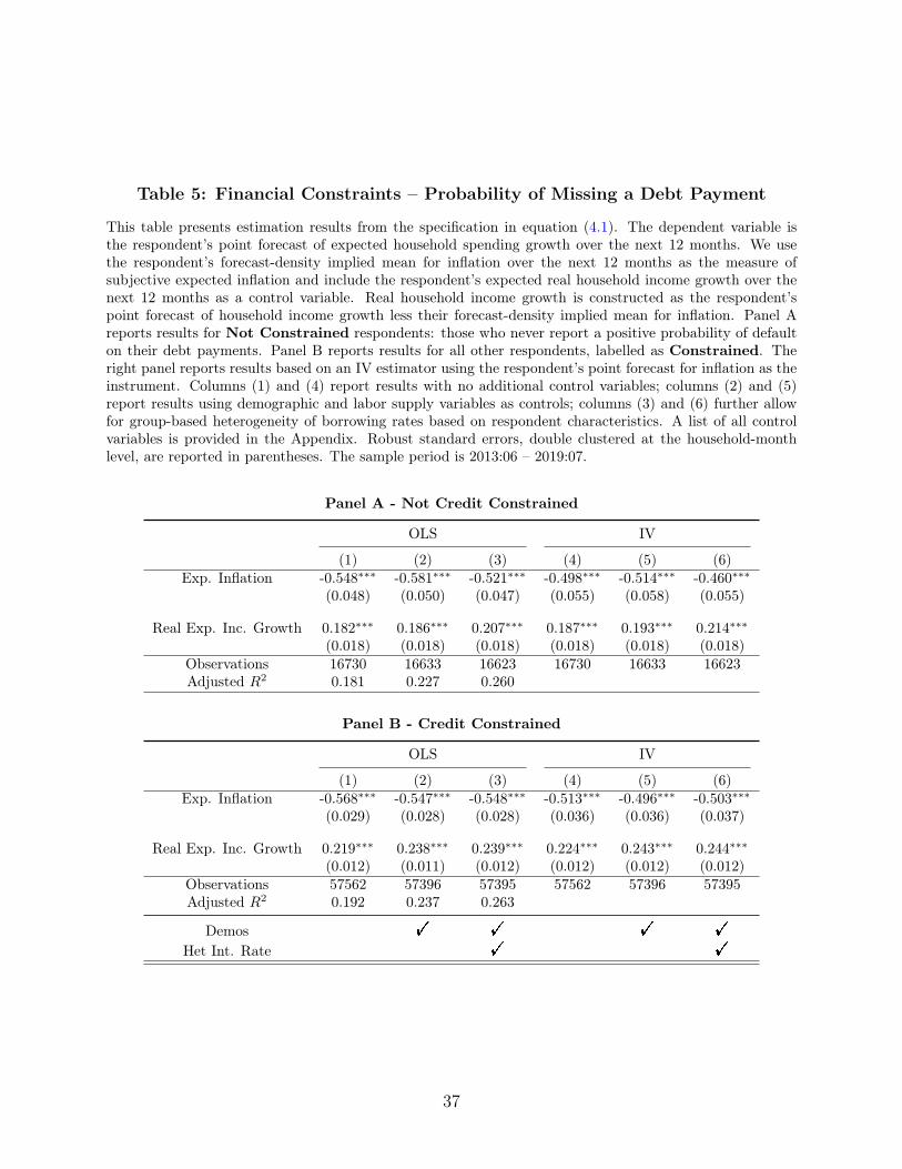
Table 5: Financial Constraints – Probability of Missing a Debt Payment

This table presents estimation results from the specification in equation (4.1). The dependent variable isthe respondent’s point forecast of expected household spending growth over the next 12 months. We usethe respondent’s forecast-density implied mean for inflation over the next 12 months as the measure ofsubjective expected inflation and include the respondent’s expected real household income growth over thenext 12 months as a control variable. Real household income growth is constructed as the respondent’spoint forecast of household income growth less their forecast-density implied mean for inflation. Panel Areports results for Not Constrained respondents: those who never report a positive probability of defaulton their debt payments. Panel B reports results for all other respondents, labelled as Constrained. Theright panel reports results based on an IV estimator using the respondent’s point forecast for inflation as theinstrument. Columns (1) and (4) report results with no additional control variables; columns (2) and (5)report results using demographic and labor supply variables as controls; columns (3) and (6) further allowfor group-based heterogeneity of borrowing rates based on respondent characteristics. A list of all controlvariables is provided in the Appendix. Robust standard errors, double clustered at the household-monthlevel, are reported in parentheses. The sample period is 2013:06 – 2019:07.

Panel A - Not Credit Constrained

OLS IV

(1) (2) (3) (4) (5) (6)Exp. Inflation -0.548∗∗∗ -0.581∗∗∗ -0.521∗∗∗ -0.498∗∗∗ -0.514∗∗∗ -0.460∗∗∗

(0.048) (0.050) (0.047) (0.055) (0.058) (0.055)

Real Exp. Inc. Growth 0.182∗∗∗ 0.186∗∗∗ 0.207∗∗∗ 0.187∗∗∗ 0.193∗∗∗ 0.214∗∗∗(0.018) (0.018) (0.018) (0.018) (0.018) (0.018)

Observations 16730 16633 16623 16730 16633 16623Adjusted R2 0.181 0.227 0.260

Panel B - Credit Constrained

OLS IV

(1) (2) (3) (4) (5) (6)Exp. Inflation -0.568∗∗∗ -0.547∗∗∗ -0.548∗∗∗ -0.513∗∗∗ -0.496∗∗∗ -0.503∗∗∗

(0.029) (0.028) (0.028) (0.036) (0.036) (0.037)

Real Exp. Inc. Growth 0.219∗∗∗ 0.238∗∗∗ 0.239∗∗∗ 0.224∗∗∗ 0.243∗∗∗ 0.244∗∗∗(0.012) (0.011) (0.012) (0.012) (0.012) (0.012)

Observations 57562 57396 57395 57562 57396 57395Adjusted R2 0.192 0.237 0.263

Demos ! ! ! !

Het Int. Rate ! !

37

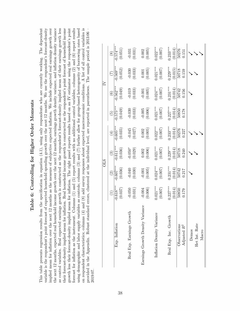
Tab

le6:

Con

trollingforHigher

Order

Mom

ents

Thistablepresents

regression

resultsfrom

thespecification

inequa

tion

(4.1),

usingon

lyrespon

dentswho

arecurrentlyworking

.The

depe

ndent

variab

leistherespon

dent’spo

intforecast

ofexpe

cted

householdspending

grow

thover

thenext

12mon

ths.

Weusetherespon

dent’sforecast-density

impliedmeanforinfla

tion

over

thene

xt12

mon

thsas

themeasure

ofsubjective

expe

cted

infla

tion

.Weinclud

eexpe

cted

real

earnings

grow

thover

thenext

12mon

ths,expe

cted

real

householdincomegrow

thover

thenext

12mon

ths,earnings

grow

thdensityvarian

ce,a

ndinfla

tion

densityvarian

ceas

controlvariab

les.

Realexpe

cted

earnings

grow

this

constructedas

therespon

dent’s

forecast-density

impliedmeanof

theirearnings

grow

thless

theirforecast-density

impliedmeanforinfla

tion

.Realh

ouseho

ldincomegrow

thisconstruc

tedas

therespon

dent’spo

intforecast

ofho

useholdincome

grow

thless

theirforecast-density

impliedmeanforinfla

tion

.The

righ

tpa

nelrepo

rtsresultsba

sedon

anIV

estimator

usingtherespon

dent’s

point

forecast

forinfla

tion

astheinstrument.

Colum

ns(1)an

d(5)repo

rtresultswithno

addition

alcontrolvariab

les;

columns

(2)an

d(6)repo

rtresults

usingdemograph

ican

dlabo

rsupp

lyvariab

lesas

controls;columns

(3)an

d(7)furtherallow

forgrou

p-ba

sedheterogeneityof

borrow

ingratesba

sed

onrespon

dent

characteristics;

columns

(4)an

d(8)ad

dsurvey

respon

sesab

outexpe

cted

macroecon

omic

cond

itions.A

listof

allcontrolvariab

lesis

provided

intheApp

endix.

Rob

uststan

dard

errors,clusteredat

theindividu

allevel,arerepo

rted

inpa

rentheses.

The

samplepe

riod

is2013:06–

2019:07.

OLS

IV

(1)

(2)

(3)

(4)

(5)

(6)

(7)

(8)

Exp

.Infla

tion

-0.618∗∗∗

-0.607∗∗∗

-0.611∗∗∗

-0.605∗∗∗

-0.575∗∗∗

-0.562∗∗∗

-0.569∗∗∗

-0.574∗∗∗

(0.037)

(0.036)

(0.036)

(0.035)

(0.049)

(0.049)

(0.052)

(0.051)

RealE

xp.Earning

sGrowth

-0.050

-0.040

-0.050∗

-0.045

-0.030

-0.019

-0.030

-0.031

(0.031)

(0.030)

(0.029)

(0.027)

(0.033)

(0.033)

(0.033)

(0.031)

Earning

sGrowth

Density

Variance

-0.004

-0.001

0.002

0.002

-0.005

-0.001

0.001

0.002

(0.006)

(0.005)

(0.006)

(0.005)

(0.006)

(0.005)

(0.005)

(0.005)

Infla

tion

Density

Varianc

e0.021∗∗∗

0.024∗∗∗

0.021∗∗∗

0.022∗∗∗

0.021∗∗∗

0.024∗∗∗

0.021∗∗∗

0.022∗∗∗

(0.007)

(0.007)

(0.007)

(0.007)

(0.007)

(0.007)

(0.007)

(0.007)

RealE

xp.Inc.

Growth

0.227∗∗∗

0.231∗∗∗

0.229∗∗∗

0.233∗∗∗

0.227∗∗∗

0.231∗∗∗

0.229∗∗∗

0.233∗∗∗

(0.014)

(0.014)

(0.014)

(0.014)

(0.014)

(0.014)

(0.015)

(0.014)

Observation

s50850

50742

50718

50276

50850

50742

50718

50276

AdjustedR

20.179

0.217

0.240

0.227

0.178

0.156

0.159

0.151

Dem

os!

!!

!!

!

Het

Int.

Rate

!!

!!

Macro

!!

38

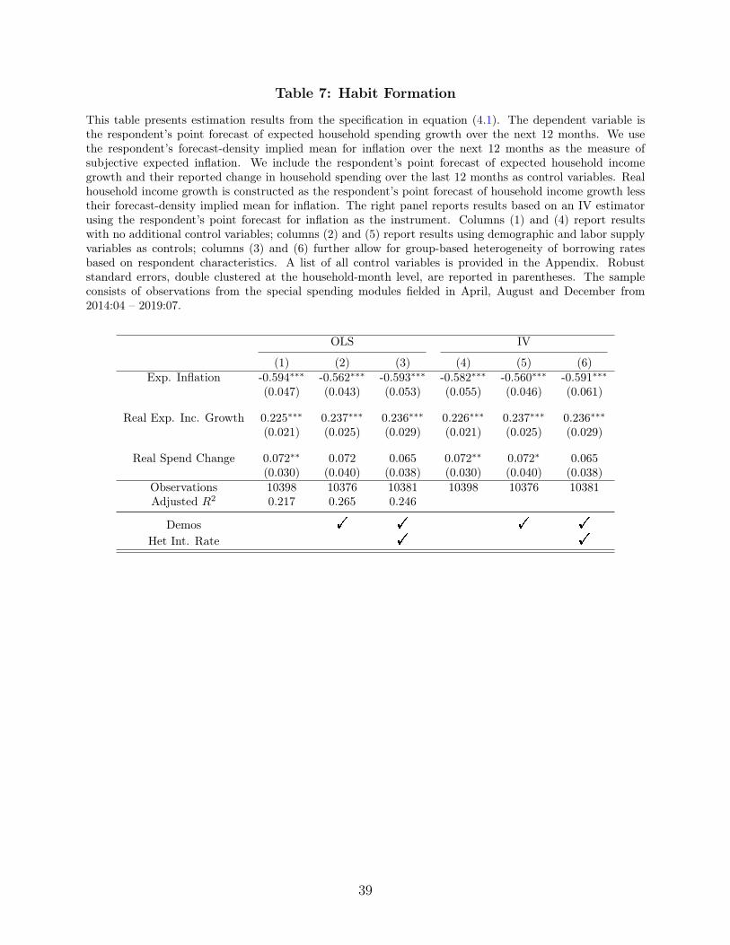
Table 7: Habit Formation

This table presents estimation results from the specification in equation (4.1). The dependent variable isthe respondent’s point forecast of expected household spending growth over the next 12 months. We usethe respondent’s forecast-density implied mean for inflation over the next 12 months as the measure ofsubjective expected inflation. We include the respondent’s point forecast of expected household incomegrowth and their reported change in household spending over the last 12 months as control variables. Realhousehold income growth is constructed as the respondent’s point forecast of household income growth lesstheir forecast-density implied mean for inflation. The right panel reports results based on an IV estimatorusing the respondent’s point forecast for inflation as the instrument. Columns (1) and (4) report resultswith no additional control variables; columns (2) and (5) report results using demographic and labor supplyvariables as controls; columns (3) and (6) further allow for group-based heterogeneity of borrowing ratesbased on respondent characteristics. A list of all control variables is provided in the Appendix. Robuststandard errors, double clustered at the household-month level, are reported in parentheses. The sampleconsists of observations from the special spending modules fielded in April, August and December from2014:04 – 2019:07.

OLS IV

(1) (2) (3) (4) (5) (6)Exp. Inflation -0.594∗∗∗ -0.562∗∗∗ -0.593∗∗∗ -0.582∗∗∗ -0.560∗∗∗ -0.591∗∗∗

(0.047) (0.043) (0.053) (0.055) (0.046) (0.061)

Real Exp. Inc. Growth 0.225∗∗∗ 0.237∗∗∗ 0.236∗∗∗ 0.226∗∗∗ 0.237∗∗∗ 0.236∗∗∗(0.021) (0.025) (0.029) (0.021) (0.025) (0.029)

Real Spend Change 0.072∗∗ 0.072 0.065 0.072∗∗ 0.072∗ 0.065(0.030) (0.040) (0.038) (0.030) (0.040) (0.038)

Observations 10398 10376 10381 10398 10376 10381Adjusted R2 0.217 0.265 0.246

Demos ! ! ! !

Het Int. Rate ! !

39

Table 8: Baseline Specification with Household Fixed Effects

This table presents estimation results from our baseline specification in equation (4.1). The dependentvariable is the respondent’s point forecast of expected household spending growth over the next 12 months.We use the respondent’s forecast-density implied mean for inflation over the next 12 months as the measure ofsubjective expected inflation. The right panel reports results based on an IV estimator using the respondent’spoint forecast for inflation as the instrument. All columns include household-level fixed effects. Columns(1) and (4) report results with no additional control variables; columns (2) and (5) report results using(time-varying) demographic and labor supply variables as controls; columns (3) and (6) further allow forgroup-based heterogeneity of borrowing rates based on respondent characteristics. A list of all controlvariables is provided in the Appendix. Robust standard errors, double clustered at the household-monthlevel, are reported in parentheses. The sample period is 2013:06 – 2019:07.

OLS IV

(1) (2) (3) (4) (5) (6)Exp. Inflation -0.911∗∗∗ -0.921∗∗∗ -0.916∗∗∗ -0.866∗∗∗ -0.878∗∗∗ -0.880∗∗∗

(0.026) (0.027) (0.028) (0.037) (0.038) (0.038)Observations 74359 74096 74085 74359 74096 74085Adjusted R2 0.486 0.498 0.529

Demos ! ! ! !

Het Int. Rate ! !

40

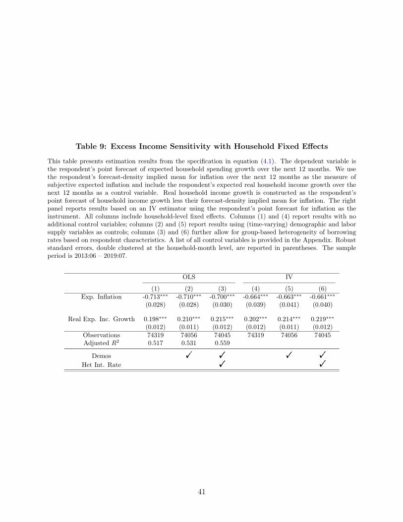
Table 9: Excess Income Sensitivity with Household Fixed Effects

This table presents estimation results from the specification in equation (4.1). The dependent variable isthe respondent’s point forecast of expected household spending growth over the next 12 months. We usethe respondent’s forecast-density implied mean for inflation over the next 12 months as the measure ofsubjective expected inflation and include the respondent’s expected real household income growth over thenext 12 months as a control variable. Real household income growth is constructed as the respondent’spoint forecast of household income growth less their forecast-density implied mean for inflation. The rightpanel reports results based on an IV estimator using the respondent’s point forecast for inflation as theinstrument. All columns include household-level fixed effects. Columns (1) and (4) report results with noadditional control variables; columns (2) and (5) report results using (time-varying) demographic and laborsupply variables as controls; columns (3) and (6) further allow for group-based heterogeneity of borrowingrates based on respondent characteristics. A list of all control variables is provided in the Appendix. Robuststandard errors, double clustered at the household-month level, are reported in parentheses. The sampleperiod is 2013:06 – 2019:07.

OLS IV

(1) (2) (3) (4) (5) (6)Exp. Inflation -0.713∗∗∗ -0.710∗∗∗ -0.700∗∗∗ -0.664∗∗∗ -0.663∗∗∗ -0.661∗∗∗

(0.028) (0.028) (0.030) (0.039) (0.041) (0.040)

Real Exp. Inc. Growth 0.198∗∗∗ 0.210∗∗∗ 0.215∗∗∗ 0.202∗∗∗ 0.214∗∗∗ 0.219∗∗∗(0.012) (0.011) (0.012) (0.012) (0.011) (0.012)

Observations 74319 74056 74045 74319 74056 74045Adjusted R2 0.517 0.531 0.559

Demos ! ! ! !

Het Int. Rate ! !

41

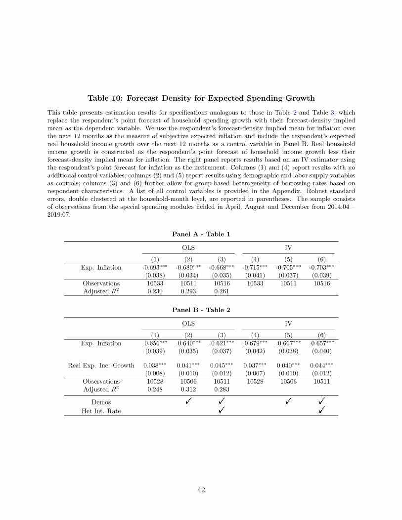
Table 10: Forecast Density for Expected Spending Growth

This table presents estimation results for specifications analogous to those in Table 2 and Table 3, whichreplace the respondent’s point forecast of household spending growth with their forecast-density impliedmean as the dependent variable. We use the respondent’s forecast-density implied mean for inflation overthe next 12 months as the measure of subjective expected inflation and include the respondent’s expectedreal household income growth over the next 12 months as a control variable in Panel B. Real householdincome growth is constructed as the respondent’s point forecast of household income growth less theirforecast-density implied mean for inflation. The right panel reports results based on an IV estimator usingthe respondent’s point forecast for inflation as the instrument. Columns (1) and (4) report results with noadditional control variables; columns (2) and (5) report results using demographic and labor supply variablesas controls; columns (3) and (6) further allow for group-based heterogeneity of borrowing rates based onrespondent characteristics. A list of all control variables is provided in the Appendix. Robust standarderrors, double clustered at the household-month level, are reported in parentheses. The sample consistsof observations from the special spending modules fielded in April, August and December from 2014:04 –2019:07.

Panel A - Table 1

OLS IV

(1) (2) (3) (4) (5) (6)Exp. Inflation -0.693∗∗∗ -0.680∗∗∗ -0.668∗∗∗ -0.715∗∗∗ -0.705∗∗∗ -0.703∗∗∗

(0.038) (0.034) (0.035) (0.041) (0.037) (0.039)Observations 10533 10511 10516 10533 10511 10516Adjusted R2 0.230 0.293 0.261

Panel B - Table 2

OLS IV

(1) (2) (3) (4) (5) (6)Exp. Inflation -0.656∗∗∗ -0.640∗∗∗ -0.621∗∗∗ -0.679∗∗∗ -0.667∗∗∗ -0.657∗∗∗

(0.039) (0.035) (0.037) (0.042) (0.038) (0.040)

Real Exp. Inc. Growth 0.038∗∗∗ 0.041∗∗∗ 0.045∗∗∗ 0.037∗∗∗ 0.040∗∗∗ 0.044∗∗∗(0.008) (0.010) (0.012) (0.007) (0.010) (0.012)

Observations 10528 10506 10511 10528 10506 10511Adjusted R2 0.248 0.312 0.283

Demos ! ! ! !

Het Int. Rate ! !

42

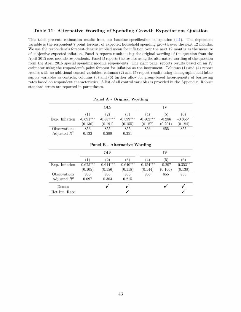
Table 11: Alternative Wording of Spending Growth Expectations Question

This table presents estimation results from our baseline specification in equation (4.1). The dependentvariable is the respondent’s point forecast of expected household spending growth over the next 12 months.We use the respondent’s forecast-density implied mean for inflation over the next 12 months as the measureof subjective expected inflation. Panel A reports results using the original wording of the question from theApril 2015 core module respondents. Panel B reports the results using the alternative wording of the questionfrom the April 2015 special spending module respondents. The right panel reports results based on an IVestimator using the respondent’s point forecast for inflation as the instrument. Columns (1) and (4) reportresults with no additional control variables; columns (2) and (5) report results using demographic and laborsupply variables as controls; columns (3) and (6) further allow for group-based heterogeneity of borrowingrates based on respondent characteristics. A list of all control variables is provided in the Appendix. Robuststandard errors are reported in parentheses.

Panel A - Original Wording

OLS IV

(1) (2) (3) (4) (5) (6)Exp. Inflation -0.691∗∗∗ -0.557∗∗∗ -0.599∗∗∗ -0.502∗∗∗ -0.286 -0.355∗

(0.130) (0.191) (0.155) (0.187) (0.201) (0.184)Observations 856 855 855 856 855 855Adjusted R2 0.132 0.299 0.251

Panel B - Alternative Wording

OLS IV

(1) (2) (3) (4) (5) (6)Exp. Inflation -0.675∗∗∗ -0.644∗∗∗ -0.640∗∗∗ -0.454∗∗∗ -0.207 -0.353∗∗

(0.105) (0.156) (0.118) (0.144) (0.166) (0.138)Observations 856 855 855 856 855 855Adjusted R2 0.097 0.303 0.215

Demos ! ! ! !

Het Int. Rate ! !

43

AppendixThe first section of the Appendix provides the exact wording for the main questions underlying the

empirical exercises in the paper.37 The second section provides details on the control variables used in thedifferent regression specifications reported in the tables.

Survey Questions

Question Q8 The next few questions are about inflation.

(a) Over the next 12 months, do you think that there will be inflation or deflation? (Note: deflationis the opposite of inflation)

# Inflation

# Deflation (the opposite of inflation)

What do you expect the rate of [inflation/deflation] to be over the next 12 months? Please give your bestguess.

(b) Over the next 12 months, I expect the rate of [inflation/deflation] to be %

Question Q9 Now we would like you to think about the different things that may happen to inflationover the next 12 months. We realize that this question may take a little more effort.

(a) In your view, what would you say is the percent chance that, over the next 12 months . . .

the rate of inflation will be 12% or higherthe rate of inflation will be between 8% and 12%the rate of inflation will be between 4% and 8%the rate of inflation will be between 2% and 4%the rate of inflation will be between 0% and 2%the rate of deflation (opposite of inflation) will be between 0% and 2%the rate of deflation (opposite of inflation) will be between 2% and 4%the rate of deflation (opposite of inflation) will be between 4% and 8%the rate of deflation (opposite of inflation) will be between 8% and 12%the rate of deflation (opposite of inflation) will be 12% or higher

percent chancepercent chancepercent chancepercent chancepercent chancepercent chancepercent chancepercent chancepercent chancepercent chance

Question Q25 Next we would like to ask you about your overall household income going forward. Byhousehold we mean everyone who usually lives in your primary residence (including yourself), excludingroommates and renters.

Over the next 12 months, what do you expect will happen to the total income of all members of yourhousehold (including you), from all sources before taxes and deductions?

37The complete questionnaire is available at http://www.newyorkfed.org/microeconomics/sce/.

44

(a) Over the next 12 months, I expect my total household income to . . .

# increase by 0% or more

# decrease by 0% or more

By about what percent do you expect your total household income to [increase/decrease]? Please give yourbest guess.

(b) Over the next 12 months, I expect my total household income to [increase/decrease] by %

Question Q26 Now think about your total household spending, including groceries, clothing, personalcare, housing (such as rent, mortgage payments, utilities, maintenance, home improvements), medical ex-penses (including health insurance), transportation, recreation and entertainment, education, and any largeitems (such as home appliances, electronics, furniture, or car payments).

Over the next 12 months, what do you expect will happen to the total spending of all members of yourhousehold (including you)?

(a) Over the next 12 months, I expect my total household spending to . . .

# increase by 0% or more

# decrease by 0% or more

By about what percent do you expect your total household spending to [increase/decrease]? Please give yourbest guess.

(b) Over the next 12 months, I expect my total household spending to [increase/decrease] by%

Question Q26 (April 2015 variant)† And now thinking of all spending categories combined,what do you think will happen to your overall monthly household spending 12 months from now, com-pared to your current monthly spending?

(a) 12 months from now, I expect my overall monthly household spending to . . .

# have increased by 0% or more

# have decreased by 0% or more

By about what percent do you expect your total household spending to [increase/decrease]? Please give yourbest guess.

(b) 12 months from now, I expect my overall monthly household spending to have [increased/decreased]by %

†This question comes immediately after a question about expenditure shares for various spending cate-gories and a question about the expected change in monthly household spending in each category 12 monthsfrom now compared to current monthly spending.

45

Question QSP6b‡ And looking ahead, how do you think your monthly household spending 12months from now, will compare to your current monthly spending in each category?

Housing (including mortgage, rent, maintenance and home owner/renter insurance) (1)Utilities (including water, sewer, electricity, gas, heating oil) (2)Food (including groceries, dining out, and beverages) (3)Clothing, footwear and personal care (4)Transportation (including gasoline, public transportation fares, and car maintenance)(5)Medical care (including health insurance, medical bills, prescription drugs) (6)Recreation and entertainment (7)Education and child care (8)Other (including gifts, child support or alimony, charitable giving, and other miscella-neous) (9)

%%%%%

%%%%

Conditioning Variables and SpecificationsHere we list the conditioning variables used as controls in our regression specifications. There are threesets of control variables: “Demos” represents demographic and labor supply variables; “Het Int. Rate”which comprises of interactions between month dummies and other variables; “Macro” which is based onexpectations about economy-wide variables.

Control Variables: Demos

Age (Categorical): 40 and below; 41-59 years old; 60 and above

Married (Indicator)

Female (Indicator)

Hispanic (Indicator)

Race (Categorical): White; Black; American Indian; Asian; Hawaiian/Pacific Islander; Other

Education (Categorical): No College; Some College/Associate’s Degree; Bachelor’s Degree

Spouse (Indicator): 0 if no spouse living in residence; 1 if one or more spouse/partner living in residence

Children Under 18 (Categorical): 0 if no children under 18 in residence; 1 if one child under 18; 2 iftwo children under 18; 3 if three or more children under 18

Children Over 18 (Indicator): 0 if no children over 18 in residence; 1 if one or more children over 18

Non-Relatives (Indicator): 0 if no non-relatives in residence; 1 if one or more non-relatives

Other Relatives - e.g. Parents/Spouses Parents (Indicator): 0 if no other relatives in residence; 1if one or more other relatives

‡ This question is from the Household Spending module. This question comes immediately after aquestion about expenditure shares for each of the spending categories. The “other” category was added inthe April 2015 survey.

46

Living Situation: This variable takes on values of all of the possible combinations of the number of:Spouses; Children over 25; Children 18-24; Children 6-17; Children younger than 6, Parents/Spouse’sParents; Other Relatives; Non-relatives

Labor Force Status: This variable takes on values of all of the possible combinations of these jobstatuses for the respondent and spouse (where No=0, Yes=1): Working full-time; Working part-time; Notworking, but would like to work; Temporarily laid off; Self-employed; On sick or other leave; Permanentlydisabled or unable to work; Retiree or early retiree; Student; Homemaker

Multiple jobs (Indicator): 0 if no job or 1 job; 1 if more than one job.

Numeracy (Indicator): 0 if low numeracy; 1 if high numeracy38

Control Variables: Het. Int. Rate

These variables include Age, Female, Race, Education, Numeracy, and Labor Force Status (as defined above)along with:

Homeownership: This variable takes on values of all of the possible combinations of two survey responses:

– Ownership of Primary Residence (Categorical): 0 if missing; 1 if respondent owns primaryresidence; 2 if respondent rents primary residence; 3 if other

– Ownership of Other Homes (Indicator)

Control Variables: Macro

Expected Unemployment The expected percent chance that the US unemployment rate will be higher12 months from now

Expected Interest Rate The expected percent change that the average interest rate on savings accountswill be higher 12 months from now

Expected Equity Values The expected percent chance that average US stock prices will be higher 12months from now

Past Credit Availability Scale from 1 (much harder) to 5 (much easier) in difficulty of obtaining creditcompared to one year ago

Future Credit Availability Scale from 1 (much harder) to 5 (much easier) in difficulty of obtainingcredit one year from now compared to present

38The numeracy measure is based on five questions in the survey about concepts such as probability andcompound interest. High numeracy respondents are designated by answering at least four questions correctly.This approach to measuring numeracy is standard (see, e.g., Lipkus, Samsa, and Rimer 2001, Lusardi 2008).

47

.

Supplementary Appendix for “Subjective Intertemporal

Substitution”

Richard K. Crump, Stefano Eusepi, Andrea Tambalotti & Giorgio Topa

The Supplementary Appendix provides additional supporting tables referenced through-out the main text:

• Tables A.1–A.4 present versions of Tables 2-5 restricted to only those respondentswho are currently employed. The control variables are identical to those in Tables2–5; however, in unreported results we include additional survey responses as controlswhich are unique to respondents who are currently employed. Specifically, we includedas additional regressors the respondent’s subjective probability of (i) losing their job inthe next 12 months, (ii) leaving their job voluntarily in the next 12 months, and (iii)finding a new job within 3 months in the hypothetical scenario where the respondentloses their job.39 We find that all of our results are fully robust to adding theseadditional regressors.

• Table A.5 is the counterpart to Table 6 with the variance of the spending growthforecast distribution as an additional regressor.

• Tables A.6–A.7 repeat the regression analyses in Tables 2–3 but for the entire untrimmedSCE sample.

• Tables A.8–A.13 present our baseline specification in equation (4.1) for subcategoriesof durable consumption growth expectations as discussed in Section 6.1.

39These questions correspond to “Q13new”, “Q14new”, and “Q22new” in the SCE core module ques-tionnaire available at https://www.newyorkfed.org/medialibrary/interactives/sce/sce/downloads/data/frbny-sce-survey-core-module-public-questionnaire.pdf.

Table A.1: Baseline Specification (Currently Employed)

This table presents estimation results from our baseline specification in equation (4.1), using only respondentswho are currently working. The dependent variable is the respondent’s point forecast of expected householdspending growth over the next 12 months. We use the respondent’s forecast-density implied mean forinflation over the next 12 months as the measure of subjective expected inflation. The right panel reportsresults based on an IV estimator using the respondent’s point forecast for inflation as the instrument.Columns (1) and (4) report results with no additional control variables; columns (2) and (5) report resultsusing demographic and labor supply variables as controls; columns (3) and (6) further allow for group-basedheterogeneity of borrowing rates based on respondent characteristics. A list of all control variables is providedin the Appendix. Robust standard errors, double clustered at the household-month level, are reported inparentheses. The sample period is 2013:06 – 2019:07.

OLS IV

(1) (2) (3) (4) (5) (6)Exp. Inflation -0.784∗∗∗ -0.785∗∗∗ -0.780∗∗∗ -0.742∗∗∗ -0.744∗∗∗ -0.740∗∗∗

(0.030) (0.030) (0.031) (0.035) (0.036) (0.038)Observations 50850 50742 50718 50850 50742 50718Adjusted R2 0.102 0.144 0.153

Demos ! ! ! !

Het Int. Rate ! !

1

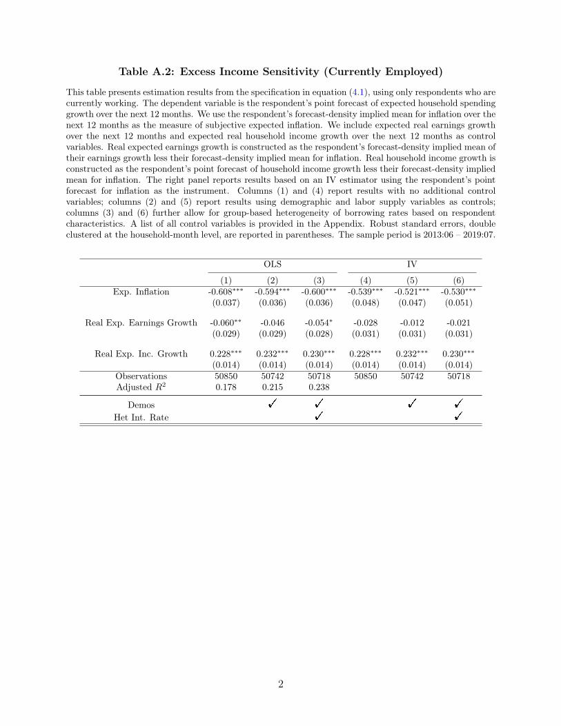
Table A.2: Excess Income Sensitivity (Currently Employed)

This table presents estimation results from the specification in equation (4.1), using only respondents who arecurrently working. The dependent variable is the respondent’s point forecast of expected household spendinggrowth over the next 12 months. We use the respondent’s forecast-density implied mean for inflation over thenext 12 months as the measure of subjective expected inflation. We include expected real earnings growthover the next 12 months and expected real household income growth over the next 12 months as controlvariables. Real expected earnings growth is constructed as the respondent’s forecast-density implied mean oftheir earnings growth less their forecast-density implied mean for inflation. Real household income growth isconstructed as the respondent’s point forecast of household income growth less their forecast-density impliedmean for inflation. The right panel reports results based on an IV estimator using the respondent’s pointforecast for inflation as the instrument. Columns (1) and (4) report results with no additional controlvariables; columns (2) and (5) report results using demographic and labor supply variables as controls;columns (3) and (6) further allow for group-based heterogeneity of borrowing rates based on respondentcharacteristics. A list of all control variables is provided in the Appendix. Robust standard errors, doubleclustered at the household-month level, are reported in parentheses. The sample period is 2013:06 – 2019:07.

OLS IV

(1) (2) (3) (4) (5) (6)Exp. Inflation -0.608∗∗∗ -0.594∗∗∗ -0.600∗∗∗ -0.539∗∗∗ -0.521∗∗∗ -0.530∗∗∗

(0.037) (0.036) (0.036) (0.048) (0.047) (0.051)

Real Exp. Earnings Growth -0.060∗∗ -0.046 -0.054∗ -0.028 -0.012 -0.021(0.029) (0.029) (0.028) (0.031) (0.031) (0.031)

Real Exp. Inc. Growth 0.228∗∗∗ 0.232∗∗∗ 0.230∗∗∗ 0.228∗∗∗ 0.232∗∗∗ 0.230∗∗∗(0.014) (0.014) (0.014) (0.014) (0.014) (0.014)

Observations 50850 50742 50718 50850 50742 50718Adjusted R2 0.178 0.215 0.238

Demos ! ! ! !

Het Int. Rate ! !

2

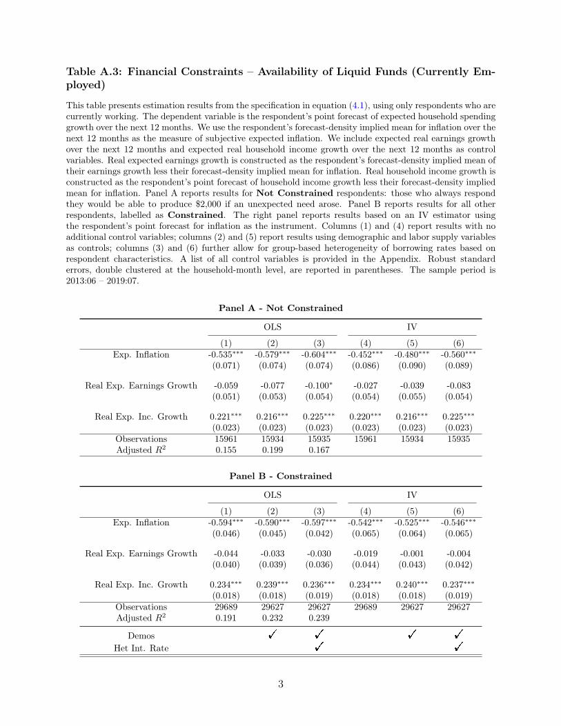
Table A.3: Financial Constraints – Availability of Liquid Funds (Currently Em-ployed)

This table presents estimation results from the specification in equation (4.1), using only respondents who arecurrently working. The dependent variable is the respondent’s point forecast of expected household spendinggrowth over the next 12 months. We use the respondent’s forecast-density implied mean for inflation over thenext 12 months as the measure of subjective expected inflation. We include expected real earnings growthover the next 12 months and expected real household income growth over the next 12 months as controlvariables. Real expected earnings growth is constructed as the respondent’s forecast-density implied mean oftheir earnings growth less their forecast-density implied mean for inflation. Real household income growth isconstructed as the respondent’s point forecast of household income growth less their forecast-density impliedmean for inflation. Panel A reports results for Not Constrained respondents: those who always respondthey would be able to produce $2,000 if an unexpected need arose. Panel B reports results for all otherrespondents, labelled as Constrained. The right panel reports results based on an IV estimator usingthe respondent’s point forecast for inflation as the instrument. Columns (1) and (4) report results with noadditional control variables; columns (2) and (5) report results using demographic and labor supply variablesas controls; columns (3) and (6) further allow for group-based heterogeneity of borrowing rates based onrespondent characteristics. A list of all control variables is provided in the Appendix. Robust standarderrors, double clustered at the household-month level, are reported in parentheses. The sample period is2013:06 – 2019:07.

Panel A - Not Constrained

OLS IV

(1) (2) (3) (4) (5) (6)Exp. Inflation -0.535∗∗∗ -0.579∗∗∗ -0.604∗∗∗ -0.452∗∗∗ -0.480∗∗∗ -0.560∗∗∗

(0.071) (0.074) (0.074) (0.086) (0.090) (0.089)

Real Exp. Earnings Growth -0.059 -0.077 -0.100∗ -0.027 -0.039 -0.083(0.051) (0.053) (0.054) (0.054) (0.055) (0.054)

Real Exp. Inc. Growth 0.221∗∗∗ 0.216∗∗∗ 0.225∗∗∗ 0.220∗∗∗ 0.216∗∗∗ 0.225∗∗∗(0.023) (0.023) (0.023) (0.023) (0.023) (0.023)

Observations 15961 15934 15935 15961 15934 15935Adjusted R2 0.155 0.199 0.167

Panel B - Constrained

OLS IV

(1) (2) (3) (4) (5) (6)Exp. Inflation -0.594∗∗∗ -0.590∗∗∗ -0.597∗∗∗ -0.542∗∗∗ -0.525∗∗∗ -0.546∗∗∗

(0.046) (0.045) (0.042) (0.065) (0.064) (0.065)

Real Exp. Earnings Growth -0.044 -0.033 -0.030 -0.019 -0.001 -0.004(0.040) (0.039) (0.036) (0.044) (0.043) (0.042)

Real Exp. Inc. Growth 0.234∗∗∗ 0.239∗∗∗ 0.236∗∗∗ 0.234∗∗∗ 0.240∗∗∗ 0.237∗∗∗(0.018) (0.018) (0.019) (0.018) (0.018) (0.019)

Observations 29689 29627 29627 29689 29627 29627Adjusted R2 0.191 0.232 0.239

Demos ! ! ! !

Het Int. Rate ! !

3

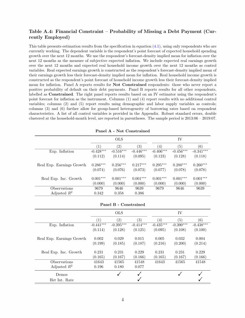
Table A.4: Financial Constraint – Probability of Missing a Debt Payment (Cur-rently Employed)

This table presents estimation results from the specification in equation (4.1), using only respondents who arecurrently working. The dependent variable is the respondent’s point forecast of expected household spendinggrowth over the next 12 months. We use the respondent’s forecast-density implied mean for inflation over thenext 12 months as the measure of subjective expected inflation. We include expected real earnings growthover the next 12 months and expected real household income growth over the next 12 months as controlvariables. Real expected earnings growth is constructed as the respondent’s forecast-density implied mean oftheir earnings growth less their forecast-density implied mean for inflation. Real household income growth isconstructed as the respondent’s point forecast of household income growth less their forecast-density impliedmean for inflation. Panel A reports results for Not Constrained respondents: those who never report apositive probability of default on their debt payments. Panel B reports results for all other respondents,labelled as Constrained. The right panel reports results based on an IV estimator using the respondent’spoint forecast for inflation as the instrument. Columns (1) and (4) report results with no additional controlvariables; columns (2) and (5) report results using demographic and labor supply variables as controls;columns (3) and (6) further allow for group-based heterogeneity of borrowing rates based on respondentcharacteristics. A list of all control variables is provided in the Appendix. Robust standard errors, doubleclustered at the household-month level, are reported in parentheses. The sample period is 2013:06 – 2019:07.

Panel A - Not Constrained

OLS IV

(1) (2) (3) (4) (5) (6)Exp. Inflation -0.428∗∗∗ -0.516∗∗∗ -0.446∗∗∗ -0.406∗∗∗ -0.456∗∗∗ -0.341∗∗∗

(0.112) (0.114) (0.095) (0.123) (0.128) (0.118)

Real Exp. Earnings Growth 0.286∗∗∗ 0.256∗∗∗ 0.217∗∗∗ 0.295∗∗∗ 0.280∗∗∗ 0.260∗∗∗(0.074) (0.076) (0.073) (0.077) (0.078) (0.078)

Real Exp. Inc. Growth 0.001∗∗∗ 0.001∗∗∗ 0.001∗∗∗ 0.001∗∗∗ 0.001∗∗∗ 0.001∗∗∗(0.000) (0.000) (0.000) (0.000) (0.000) (0.000)

Observations 9679 9646 9639 9679 9646 9639Adjusted R2 0.342 0.358 0.386

Panel B - Constrained

OLS IV

(1) (2) (3) (4) (5) (6)Exp. Inflation -0.441∗∗∗ -0.395∗∗∗ -0.414∗∗∗ -0.435∗∗∗ -0.390∗∗∗ -0.438∗∗∗

(0.114) (0.128) (0.125) (0.095) (0.108) (0.100)

Real Exp. Earnings Growth 0.002 0.029 0.015 0.005 0.032 0.004(0.199) (0.185) (0.187) (0.216) (0.200) (0.214)

Real Exp. Inc. Growth 0.231 0.231 0.229 0.231 0.231 0.229(0.165) (0.167) (0.166) (0.165) (0.167) (0.166)

Observations 41643 41565 41548 41643 41565 41548Adjusted R2 0.196 0.180 0.077

Demos ! ! ! !

Het Int. Rate ! !

4

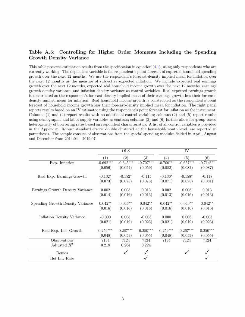
Table A.5: Controlling for Higher Order Moments Including the SpendingGrowth Density Variance

This table presents estimation results from the specification in equation (4.1), using only respondents who arecurrently working. The dependent variable is the respondent’s point forecast of expected household spendinggrowth over the next 12 months. We use the respondent’s forecast-density implied mean for inflation overthe next 12 months as the measure of subjective expected inflation. We include expected real earningsgrowth over the next 12 months, expected real household income growth over the next 12 months, earningsgrowth density variance, and inflation density variance as control variables. Real expected earnings growthis constructed as the respondent’s forecast-density implied mean of their earnings growth less their forecast-density implied mean for inflation. Real household income growth is constructed as the respondent’s pointforecast of household income growth less their forecast-density implied mean for inflation. The right panelreports results based on an IV estimator using the respondent’s point forecast for inflation as the instrument.Columns (1) and (4) report results with no additional control variables; columns (2) and (5) report resultsusing demographic and labor supply variables as controls; columns (3) and (6) further allow for group-basedheterogeneity of borrowing rates based on respondent characteristics. A list of all control variables is providedin the Appendix. Robust standard errors, double clustered at the household-month level, are reported inparentheses. The sample consists of observations from the special spending modules fielded in April, Augustand December from 2014:04 – 2019:07.

OLS IV

(1) (2) (3) (4) (5) (6)Exp. Inflation -0.692∗∗∗ -0.645∗∗∗ -0.707∗∗∗ -0.700∗∗∗ -0.657∗∗∗ -0.714∗∗∗

(0.056) (0.054) (0.059) (0.082) (0.082) (0.087)

Real Exp. Earnings Growth -0.132∗ -0.152∗ -0.115 -0.136∗ -0.158∗ -0.118(0.073) (0.075) (0.075) (0.071) (0.075) (0.081)

Earnings Growth Density Variance 0.002 0.008 0.013 0.002 0.008 0.013(0.014) (0.016) (0.013) (0.013) (0.016) (0.013)

Spending Growth Density Variance 0.042∗∗ 0.046∗∗ 0.042∗∗ 0.042∗∗ 0.046∗∗ 0.042∗∗(0.016) (0.016) (0.016) (0.016) (0.016) (0.016)

Inflation Density Variance -0.000 0.008 -0.003 0.000 0.008 -0.003(0.021) (0.019) (0.023) (0.021) (0.019) (0.023)

Real Exp. Inc. Growth 0.259∗∗∗ 0.267∗∗∗ 0.250∗∗∗ 0.259∗∗∗ 0.267∗∗∗ 0.250∗∗∗(0.048) (0.053) (0.055) (0.048) (0.053) (0.055)

Observations 7134 7124 7124 7134 7124 7124Adjusted R2 0.218 0.264 0.224

Demos ! ! ! !

Het Int. Rate ! !

5

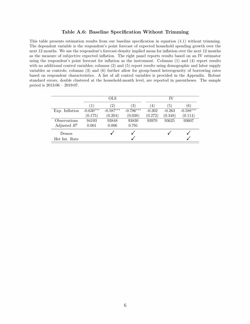
Table A.6: Baseline Specification Without Trimming

This table presents estimation results from our baseline specification in equation (4.1) without trimming.The dependent variable is the respondent’s point forecast of expected household spending growth over thenext 12 months. We use the respondent’s forecast-density implied mean for inflation over the next 12 monthsas the measure of subjective expected inflation. The right panel reports results based on an IV estimatorusing the respondent’s point forecast for inflation as the instrument. Columns (1) and (4) report resultswith no additional control variables; columns (2) and (5) report results using demographic and labor supplyvariables as controls; columns (3) and (6) further allow for group-based heterogeneity of borrowing ratesbased on respondent characteristics. A list of all control variables is provided in the Appendix. Robuststandard errors, double clustered at the household-month level, are reported in parentheses. The sampleperiod is 2013:06 – 2019:07.

OLS IV

(1) (2) (3) (4) (5) (6)Exp. Inflation -0.630∗∗∗ -0.587∗∗∗ -0.796∗∗∗ -0.302 -0.263 -0.588∗∗∗

(0.175) (0.204) (0.038) (0.272) (0.348) (0.114)Observations 94193 93848 93830 93970 93625 93607Adjusted R2 0.001 0.006 0.791

Demos ! ! ! !

Het Int. Rate ! !

6

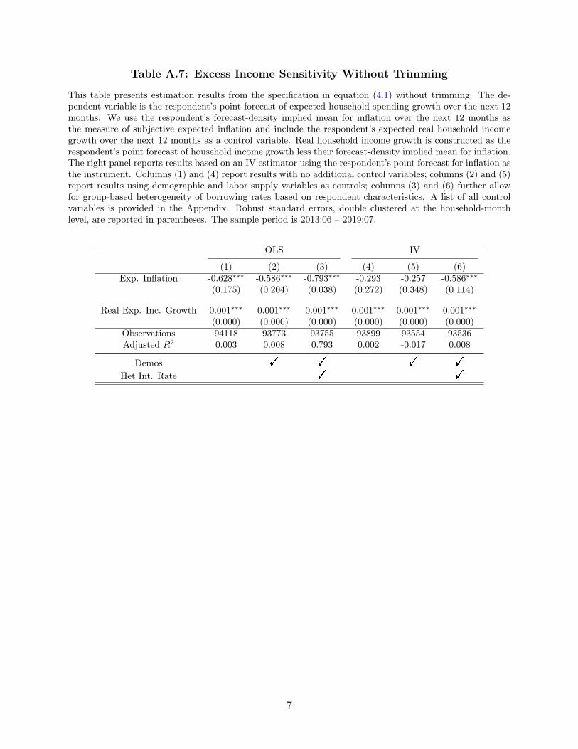
Table A.7: Excess Income Sensitivity Without Trimming

This table presents estimation results from the specification in equation (4.1) without trimming. The de-pendent variable is the respondent’s point forecast of expected household spending growth over the next 12months. We use the respondent’s forecast-density implied mean for inflation over the next 12 months asthe measure of subjective expected inflation and include the respondent’s expected real household incomegrowth over the next 12 months as a control variable. Real household income growth is constructed as therespondent’s point forecast of household income growth less their forecast-density implied mean for inflation.The right panel reports results based on an IV estimator using the respondent’s point forecast for inflation asthe instrument. Columns (1) and (4) report results with no additional control variables; columns (2) and (5)report results using demographic and labor supply variables as controls; columns (3) and (6) further allowfor group-based heterogeneity of borrowing rates based on respondent characteristics. A list of all controlvariables is provided in the Appendix. Robust standard errors, double clustered at the household-monthlevel, are reported in parentheses. The sample period is 2013:06 – 2019:07.

OLS IV

(1) (2) (3) (4) (5) (6)Exp. Inflation -0.628∗∗∗ -0.586∗∗∗ -0.793∗∗∗ -0.293 -0.257 -0.586∗∗∗

(0.175) (0.204) (0.038) (0.272) (0.348) (0.114)

Real Exp. Inc. Growth 0.001∗∗∗ 0.001∗∗∗ 0.001∗∗∗ 0.001∗∗∗ 0.001∗∗∗ 0.001∗∗∗(0.000) (0.000) (0.000) (0.000) (0.000) (0.000)

Observations 94118 93773 93755 93899 93554 93536Adjusted R2 0.003 0.008 0.793 0.002 -0.017 0.008

Demos ! ! ! !

Het Int. Rate ! !

7

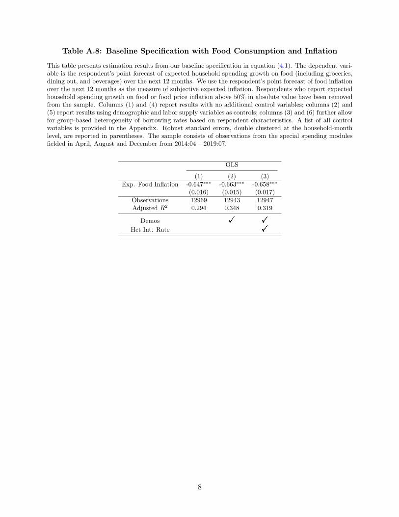
Table A.8: Baseline Specification with Food Consumption and Inflation

This table presents estimation results from our baseline specification in equation (4.1). The dependent vari-able is the respondent’s point forecast of expected household spending growth on food (including groceries,dining out, and beverages) over the next 12 months. We use the respondent’s point forecast of food inflationover the next 12 months as the measure of subjective expected inflation. Respondents who report expectedhousehold spending growth on food or food price inflation above 50% in absolute value have been removedfrom the sample. Columns (1) and (4) report results with no additional control variables; columns (2) and(5) report results using demographic and labor supply variables as controls; columns (3) and (6) further allowfor group-based heterogeneity of borrowing rates based on respondent characteristics. A list of all controlvariables is provided in the Appendix. Robust standard errors, double clustered at the household-monthlevel, are reported in parentheses. The sample consists of observations from the special spending modulesfielded in April, August and December from 2014:04 – 2019:07.

OLS

(1) (2) (3)Exp. Food Inflation -0.647∗∗∗ -0.663∗∗∗ -0.658∗∗∗

(0.016) (0.015) (0.017)Observations 12969 12943 12947Adjusted R2 0.294 0.348 0.319

Demos ! !

Het Int. Rate !

8

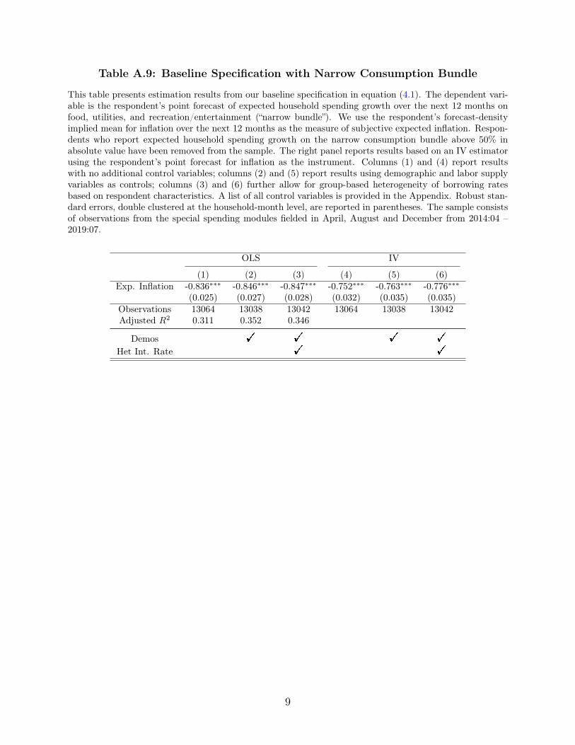
Table A.9: Baseline Specification with Narrow Consumption Bundle

This table presents estimation results from our baseline specification in equation (4.1). The dependent vari-able is the respondent’s point forecast of expected household spending growth over the next 12 months onfood, utilities, and recreation/entertainment (“narrow bundle”). We use the respondent’s forecast-densityimplied mean for inflation over the next 12 months as the measure of subjective expected inflation. Respon-dents who report expected household spending growth on the narrow consumption bundle above 50% inabsolute value have been removed from the sample. The right panel reports results based on an IV estimatorusing the respondent’s point forecast for inflation as the instrument. Columns (1) and (4) report resultswith no additional control variables; columns (2) and (5) report results using demographic and labor supplyvariables as controls; columns (3) and (6) further allow for group-based heterogeneity of borrowing ratesbased on respondent characteristics. A list of all control variables is provided in the Appendix. Robust stan-dard errors, double clustered at the household-month level, are reported in parentheses. The sample consistsof observations from the special spending modules fielded in April, August and December from 2014:04 –2019:07.

OLS IV

(1) (2) (3) (4) (5) (6)Exp. Inflation -0.836∗∗∗ -0.846∗∗∗ -0.847∗∗∗ -0.752∗∗∗ -0.763∗∗∗ -0.776∗∗∗

(0.025) (0.027) (0.028) (0.032) (0.035) (0.035)Observations 13064 13038 13042 13064 13038 13042Adjusted R2 0.311 0.352 0.346

Demos ! ! ! !

Het Int. Rate ! !

9

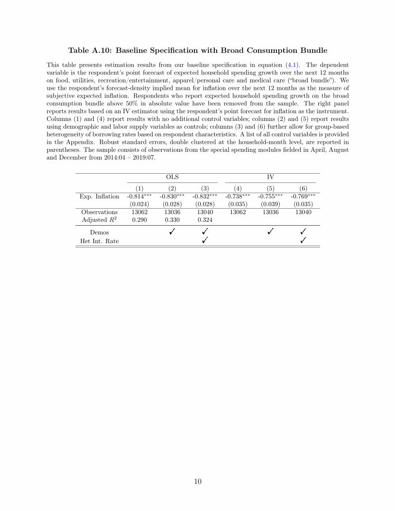
Table A.10: Baseline Specification with Broad Consumption Bundle

This table presents estimation results from our baseline specification in equation (4.1). The dependentvariable is the respondent’s point forecast of expected household spending growth over the next 12 monthson food, utilities, recreation/entertainment, apparel/personal care and medical care (“broad bundle”). Weuse the respondent’s forecast-density implied mean for inflation over the next 12 months as the measure ofsubjective expected inflation. Respondents who report expected household spending growth on the broadconsumption bundle above 50% in absolute value have been removed from the sample. The right panelreports results based on an IV estimator using the respondent’s point forecast for inflation as the instrument.Columns (1) and (4) report results with no additional control variables; columns (2) and (5) report resultsusing demographic and labor supply variables as controls; columns (3) and (6) further allow for group-basedheterogeneity of borrowing rates based on respondent characteristics. A list of all control variables is providedin the Appendix. Robust standard errors, double clustered at the household-month level, are reported inparentheses. The sample consists of observations from the special spending modules fielded in April, Augustand December from 2014:04 – 2019:07.

OLS IV

(1) (2) (3) (4) (5) (6)Exp. Inflation -0.814∗∗∗ -0.830∗∗∗ -0.832∗∗∗ -0.738∗∗∗ -0.755∗∗∗ -0.769∗∗∗

(0.024) (0.028) (0.028) (0.035) (0.039) (0.035)Observations 13062 13036 13040 13062 13036 13040Adjusted R2 0.290 0.330 0.324

Demos ! ! ! !

Het Int. Rate ! !

10

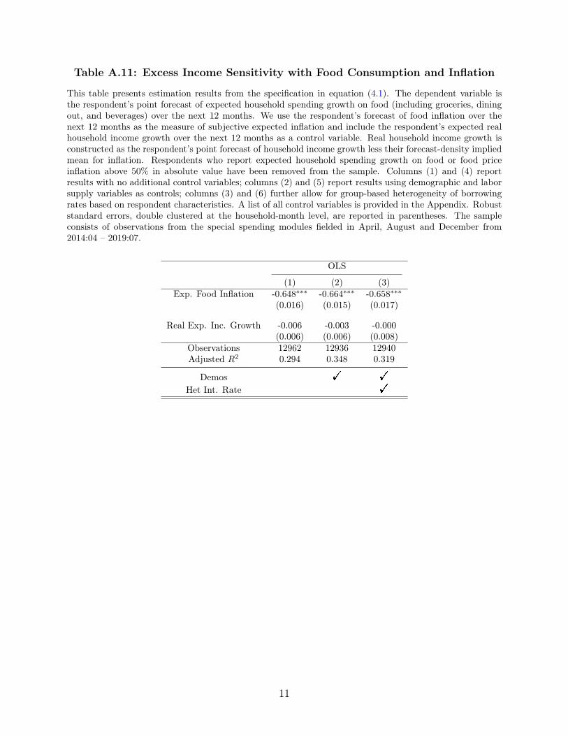
Table A.11: Excess Income Sensitivity with Food Consumption and Inflation

This table presents estimation results from the specification in equation (4.1). The dependent variable isthe respondent’s point forecast of expected household spending growth on food (including groceries, diningout, and beverages) over the next 12 months. We use the respondent’s forecast of food inflation over thenext 12 months as the measure of subjective expected inflation and include the respondent’s expected realhousehold income growth over the next 12 months as a control variable. Real household income growth isconstructed as the respondent’s point forecast of household income growth less their forecast-density impliedmean for inflation. Respondents who report expected household spending growth on food or food priceinflation above 50% in absolute value have been removed from the sample. Columns (1) and (4) reportresults with no additional control variables; columns (2) and (5) report results using demographic and laborsupply variables as controls; columns (3) and (6) further allow for group-based heterogeneity of borrowingrates based on respondent characteristics. A list of all control variables is provided in the Appendix. Robuststandard errors, double clustered at the household-month level, are reported in parentheses. The sampleconsists of observations from the special spending modules fielded in April, August and December from2014:04 – 2019:07.

OLS

(1) (2) (3)Exp. Food Inflation -0.648∗∗∗ -0.664∗∗∗ -0.658∗∗∗

(0.016) (0.015) (0.017)

Real Exp. Inc. Growth -0.006 -0.003 -0.000(0.006) (0.006) (0.008)

Observations 12962 12936 12940Adjusted R2 0.294 0.348 0.319

Demos ! !

Het Int. Rate !

11

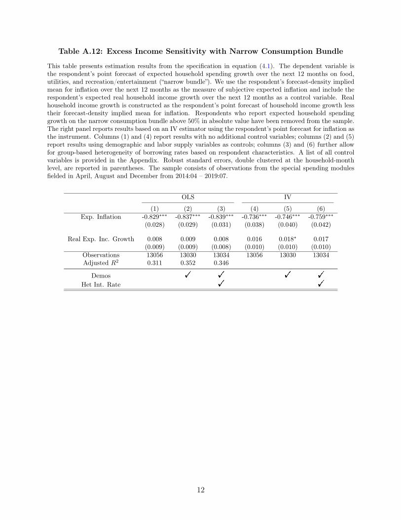
Table A.12: Excess Income Sensitivity with Narrow Consumption Bundle

This table presents estimation results from the specification in equation (4.1). The dependent variable isthe respondent’s point forecast of expected household spending growth over the next 12 months on food,utilities, and recreation/entertainment (“narrow bundle”). We use the respondent’s forecast-density impliedmean for inflation over the next 12 months as the measure of subjective expected inflation and include therespondent’s expected real household income growth over the next 12 months as a control variable. Realhousehold income growth is constructed as the respondent’s point forecast of household income growth lesstheir forecast-density implied mean for inflation. Respondents who report expected household spendinggrowth on the narrow consumption bundle above 50% in absolute value have been removed from the sample.The right panel reports results based on an IV estimator using the respondent’s point forecast for inflation asthe instrument. Columns (1) and (4) report results with no additional control variables; columns (2) and (5)report results using demographic and labor supply variables as controls; columns (3) and (6) further allowfor group-based heterogeneity of borrowing rates based on respondent characteristics. A list of all controlvariables is provided in the Appendix. Robust standard errors, double clustered at the household-monthlevel, are reported in parentheses. The sample consists of observations from the special spending modulesfielded in April, August and December from 2014:04 – 2019:07.

OLS IV

(1) (2) (3) (4) (5) (6)Exp. Inflation -0.829∗∗∗ -0.837∗∗∗ -0.839∗∗∗ -0.736∗∗∗ -0.746∗∗∗ -0.759∗∗∗

(0.028) (0.029) (0.031) (0.038) (0.040) (0.042)

Real Exp. Inc. Growth 0.008 0.009 0.008 0.016 0.018∗ 0.017(0.009) (0.009) (0.008) (0.010) (0.010) (0.010)

Observations 13056 13030 13034 13056 13030 13034Adjusted R2 0.311 0.352 0.346

Demos ! ! ! !

Het Int. Rate ! !

12

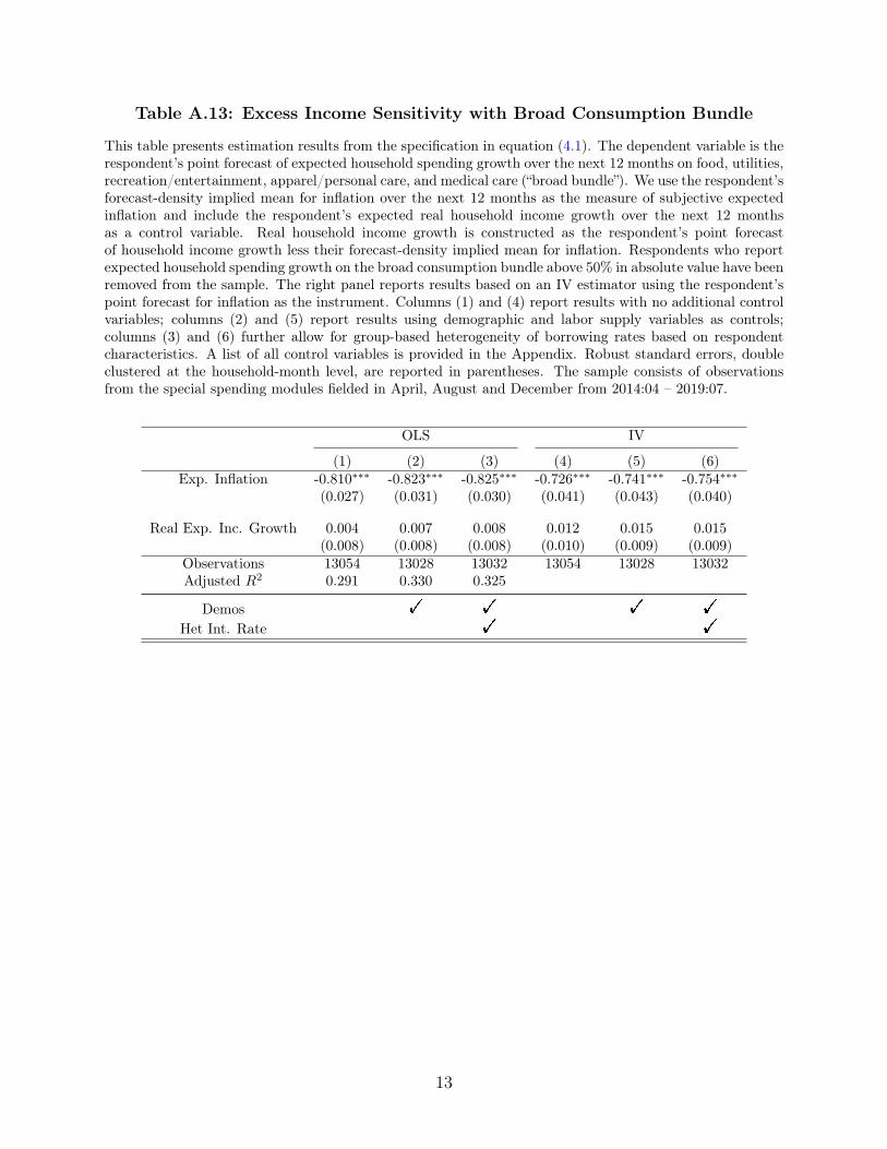
Table A.13: Excess Income Sensitivity with Broad Consumption Bundle

This table presents estimation results from the specification in equation (4.1). The dependent variable is therespondent’s point forecast of expected household spending growth over the next 12 months on food, utilities,recreation/entertainment, apparel/personal care, and medical care (“broad bundle”). We use the respondent’sforecast-density implied mean for inflation over the next 12 months as the measure of subjective expectedinflation and include the respondent’s expected real household income growth over the next 12 monthsas a control variable. Real household income growth is constructed as the respondent’s point forecastof household income growth less their forecast-density implied mean for inflation. Respondents who reportexpected household spending growth on the broad consumption bundle above 50% in absolute value have beenremoved from the sample. The right panel reports results based on an IV estimator using the respondent’spoint forecast for inflation as the instrument. Columns (1) and (4) report results with no additional controlvariables; columns (2) and (5) report results using demographic and labor supply variables as controls;columns (3) and (6) further allow for group-based heterogeneity of borrowing rates based on respondentcharacteristics. A list of all control variables is provided in the Appendix. Robust standard errors, doubleclustered at the household-month level, are reported in parentheses. The sample consists of observationsfrom the special spending modules fielded in April, August and December from 2014:04 – 2019:07.

OLS IV

(1) (2) (3) (4) (5) (6)Exp. Inflation -0.810∗∗∗ -0.823∗∗∗ -0.825∗∗∗ -0.726∗∗∗ -0.741∗∗∗ -0.754∗∗∗

(0.027) (0.031) (0.030) (0.041) (0.043) (0.040)

Real Exp. Inc. Growth 0.004 0.007 0.008 0.012 0.015 0.015(0.008) (0.008) (0.008) (0.010) (0.009) (0.009)

Observations 13054 13028 13032 13054 13028 13032Adjusted R2 0.291 0.330 0.325

Demos ! ! ! !

Het Int. Rate ! !

13