SU326 P30-64

THE MATRIX INVERSE EIGENVALUE PROBLEM FORPERIODIC JACOBI MATRICES

bY

D. L. Boley and G. H. Golub

STAN-CS-78-684DECEMBER 19 78

COMPUTER SCIENCE DEPARTMENTSchool of Humanities and Sciences

STANFORD UNIVERSITY

su326 ~30-63

THE MATRIX INVERSE EIGEN-VALUE PROBLEM

FOR PERIODIC JACOBI MATRICES

D. L. Boley and G. H. Golub

Computer Science DepartmentStanford UniversityStanford, CA Y4305

(415) 497-3124.

This work was supported in part by Department of Energy contractEY-76-S-03-0326 PA #30MCS75-13497-AOl.

and by National Science Foundation grant

Invited paper presented at The Fourth Conference on Basic Problemsof Numerical Analysis, (LIBLICE IV), Pilsen, Czech., September 1978.

Abstract

A stable numerical algorithm is presented for generating a periodic

Jacobi matrix from two sets of eigenvalues and the product of the off-

diagonal elements of the matrix. The algorithm requires a simple

generalization of the Lanczos algorithm. It is shown that the matrix is

not unique, but the algorithm will generate all possible solutions.

q

THE MATRIX INVERSE EIGENVALUE PROBLEM

FOR PERIODIC JACOBI MATRICES

D.L. Boley and G.H. Golub

Computer Science Department, Stanford University,

Stanford, CA 94305

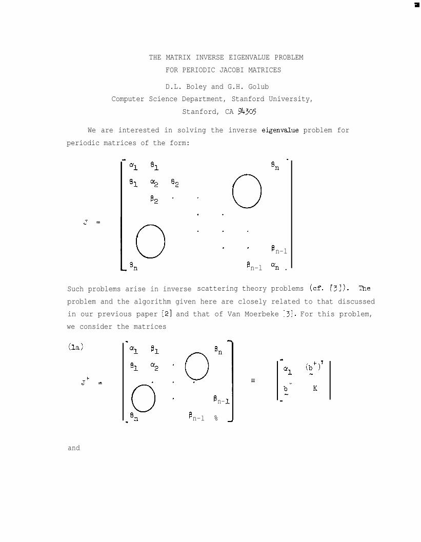
We are interested in solving the inverse eigenvalue problem for

periodic matrices of the form:

Such problems arise in inverse scattering theory problems ( fc . c31L

. . 8n-l

Bn-l % .

The

problem and the algorithm given here are closely related to that discussed

in our previous paper [2] and that of Van Moerbeke [3]. For this problem,

we consider the matrices

J+ =

Bn-l

f3n-

%

b+ Kh,

-

and

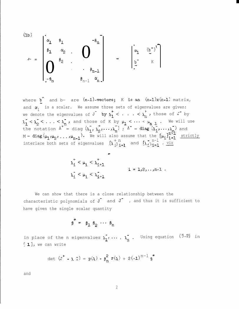
(lb)

J- =

.

5 81

g1 Q2 l

0 82 l

.

-43

0.' k-1

fJ Q;1,n-l

=

.

%

b-NL

where bf and b- are (n-1Lvectors; K isanN

- 1b )N

K

(n-l>x(n-1) matrix,

and Q1is a scalar. We assume three sets of eigenvalues are given:

we denote the eigenvalues of Jf by 1: < . . . < 1,: f those of J- by

⌧; < h; < l l l =c 1; ) and those of K by pl < ..* < pn 1 . We will use

the notation At = diag (~1, &=.~,~n) ; A- = diag (h;,=*=,h,) and

M = d-N (PlJP2Y l l l ‘P,,4 ). We will also assume that the {+]n?i strictly

interlace both sets of eigenvalues+ n

CA 3i i=land -cx 3

n-l , vizii=1 -

We can show that there is a close relationship between the

characteristic polynomials of Jf and J- , and thus it is sufficient to

have given the single scalar quantity

in place of the n eigenvalues A;, .*. , X-n . Using equation (5.2) in

[ 11, we can write

det (Jf - x I> = p(h) - BE r(h) + 2(-l)n-l *

13

and

2

det (J- - h I) = p(l) - ei r(A) - 2(-l)n-l *

@

where P(h) is the characteristic polynomial of the matrix obtained from

Jf or J- by setting p, = 0 , and r(l) is the characteristic poly-

nomial of the submatrix consisting of rows and columns 2,3,...,n-1 of the

matrix Jf or J- S By subtracting these two expressions we obtain

(2) det (J' _ x I) = det (Jf - h I) + 4 (-lJn B* '

We will see-the values 1; appear only as the product (h; - A)..$ - 1) ,+ + *

so that if we are given the values ll, 'n. . . , as well as p , then we do

-not need explicitly the values XIY��Yhn l

Note that the roles of 1; and of are essentially interchangeable at+

several stages, and we have made the choice to use A.1as much as possible.

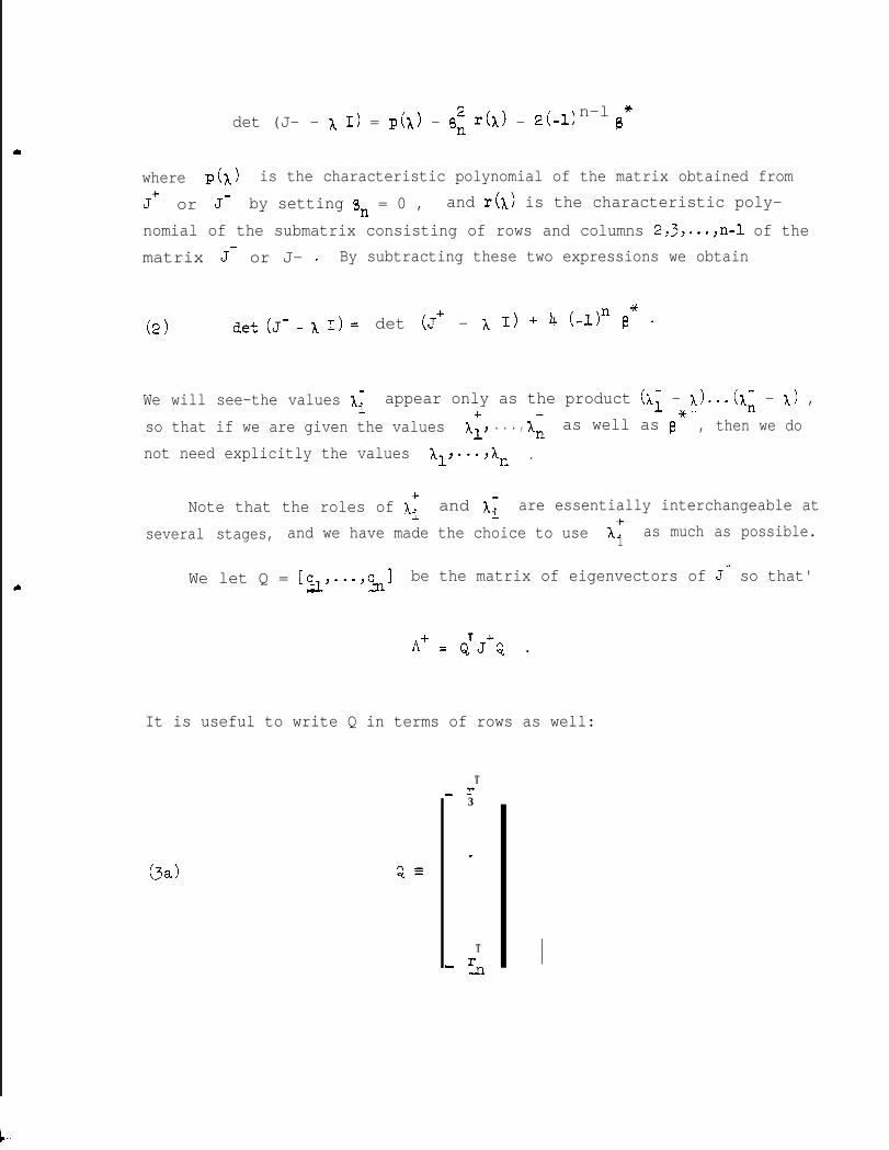
We let Q = [~,~.=,s ] be the matrix of eigenvectors of Jt so that'

A+ = QTJ+Q .

It is useful to write Q in terms of rows as well:

(3 )a QG

T- r

3

.

T

- EnI .

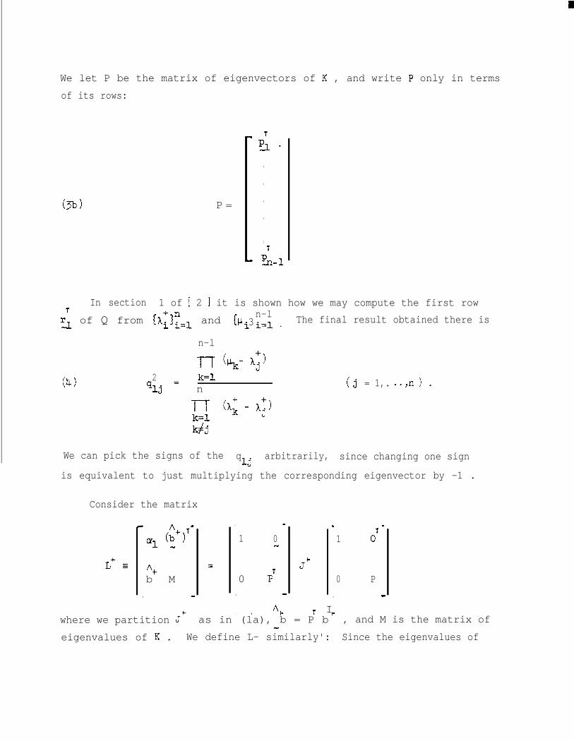
We let P be the matrix of eigenvectors of K , and write P only in terms

of its rows:

(3-d P =

- P; .

.

.

.

.

,

PT- d-1

In section 1 of [ 2 I it is shown how we may compute the first row

r; of Q from ($nl and CP 3n-l

i i=l l

The final result obtained there is

n-l

(4)2 k=l

'lj = n (j = 1,. ..,n) .

We can pick the signs of the q13

arbitrarily, since changing one sign

is equivalent to just multiplying the corresponding eigenvector by -1 .

Consider the matrix

A+b M

=

. I

-+

. m

1 0w

0 P'. a

I \ 4-

J+

t I

. m

1 OT

0 P

. m

1 -I-

where we partition J as in (la), b = P b , and M is the matrix ofCI

eigenvalues of K . We define L- similarly': Since the eigenvalues of

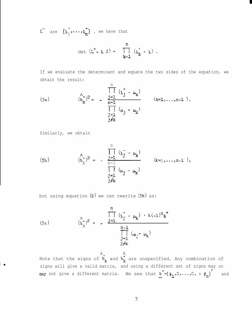
Lf Ch+ +

are 1Y'**Y 423, we have that

det CL+‘- h I> = l%+'k - x) '

k=l

If we evaluate the determinant and equate the two sides of the equation, we

obtain the result:n

(5 1aA 1 1 (+2

- l.LkJb > j=lk = - n=l (k=l,...,n-1 1.

T-l (/.L. - b)j=l J

jfk

Similarly, we obtain

n

(5b) A- 2 h)b > =k n-l (k 1= y... ,n-1 ),

7-r (p. - CLk)

j=l J

jfk

but using equation (2) we can rewrite (5b) as:

(5 )C A- 2b > =k -

i; ( )j=l

@j- Pk

jfk

A A+Note that the signs of bk and bk are unspecified. Any combination of

signs will give a valid matrix, and using a different set of signs may or

may not give a different matrix. We see that b+=[~lyOy=O~yOy + e,]' andN

5

b- =CI

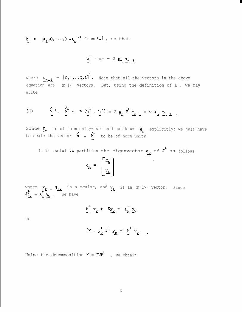
[~l,o,...,~,-~n]T from (1) , so that

bC - b- = 2 8, eA 1w

where Lo1 = [O,...,O,llT l Note that all the vectors in the above

equation are (n-l>- vectors. But, using the definition of L , we may

write

(6) :: +- ;- = P'(b+ - b-)N Y N N

= 2 B, P' eJ1 1 =2 pn s-1 l

Since PA is of norm unity- we need not know pn explicitly; we just have

to scale the vector 6'. I?- to be of norm unity.N

It is useful to partition the eigenvector qA of Jf as follows

where% = 91k

is a scalar, and yLk

is an (n-l>- vector. Since

J;& = A; 3 , we have

or

Using the decomposition K = PMPT , we obtain

6

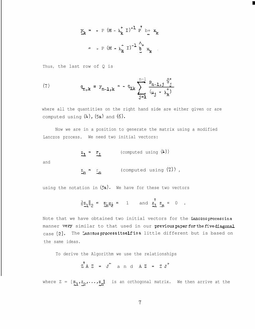
yJr= - P (M - A; I)-' P' b+ \N

= 0 P (M - 1; I&+2%

.

Thus, the last row of Q is

(7)

n-l

4-n& E yn-l,k = - ‘lk )j=l

+'n-1 j 6

Y j

(Pj - 1;)

where all the quantities on the right hand side are either given or are

computed using (4), (5a> and (6).

Now we are in a position to generate the matrix using a modified

Lanczos process. We need two initial vectors:

(computed using (4))

and

cn= r (computed using (7)) ,

using the notation in (3a>. We have for these two vectors

II IIrz12= zd2= 1II II and zTns.z_n= 0 .

Note that we have obtained two initial vectors for the La,.nczos process in a

manner very similar to that used in our previ.ous paper for the five diagonal

case [2]. The Ianczos process itself is a little different but is based on

the same ideas.

To derive the Algorithm we use the relationships

ZTAZ=J+ a n d AZ=ZJ+

where Z = [zJY~Y"'Y31z 1 is an orthogonal matrix. We then arrive at the

7

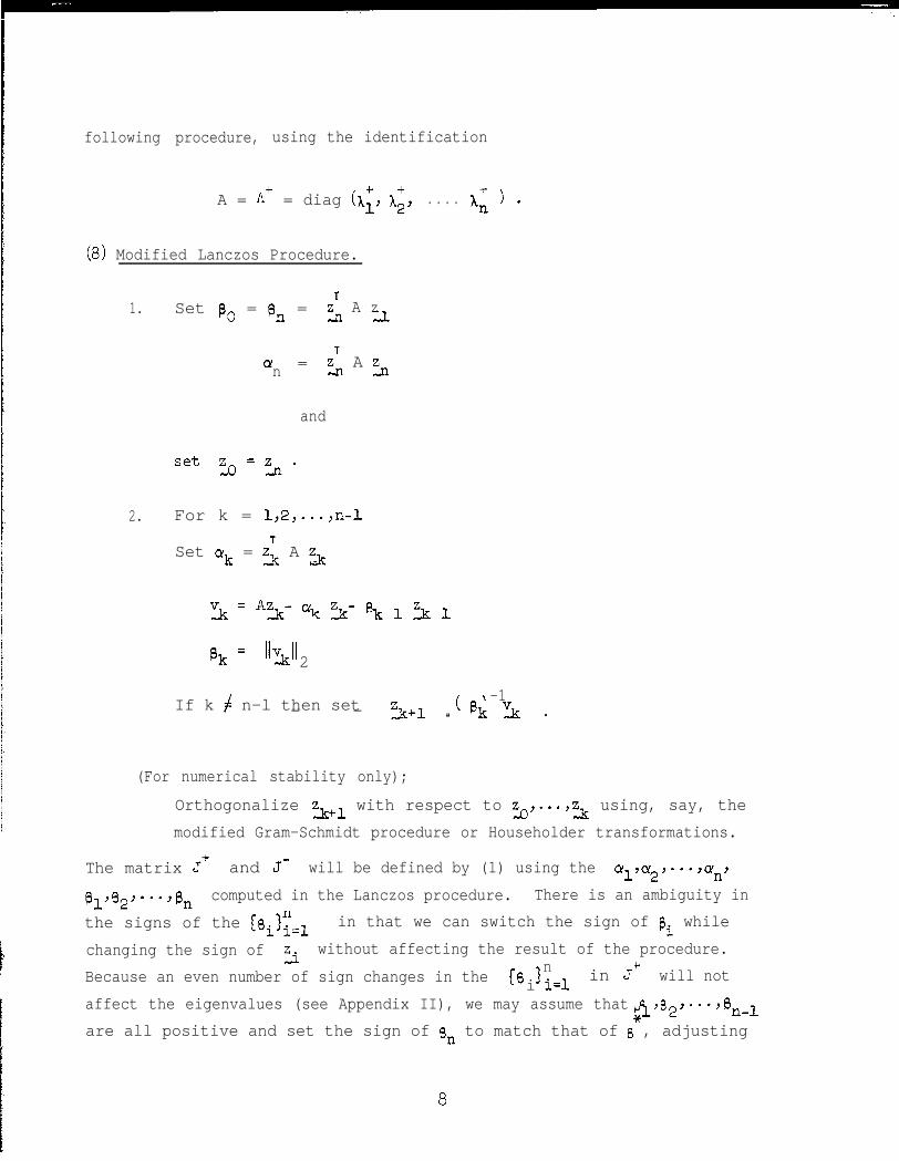
following procedure, using the identification

A = A' = diag (~1, A:, . . . .

(8) Modified Lanczos Procedure.

1. Set p. = p, = z; A z2

cy =nz; A Z~

and

set z,o = En '

2. For k = 1,2,...,n-1

Set ak = z; A z~

3s = Ay CY’tc zy Bk 1 5 1

Bk = II IIEk 2

If k f n-l then set ( >-1

- - �A+1 = & v& l

(For numerical stability only);

Orthogonalize z~+~ with respect to z~,...,z~ using, say, the

modified Gram-Schmidt procedure or Householder transformations.

The matrix Jf and J- will be defined by (1) using the CY ,a12,=**,an,

81’Bp’-‘Bn computed in the Lanczos procedure. There is an ambiguity in

the signs of the [pi]?1 in that we can switch the sign of pi while

changing the sign ofEi

without affecting the result of the procedure.

Because an even number of sign changes in the CB 3n in J

ti i=l

will not

affect the eigenvalues (see Appendix II), we may assume that B ,g,1 2"*'*"@n-1are all positive and set the sign of 8n to match that of e , adjusting

8

the vector Z~ accordingly.

To summarize the Algorithm:

We are given two sets of eigenvalues

+ ncx 3 c In-l

ii=1 ' Pi i=l

*and the scalar e .

1.

2.

3.

4.

50

Compute zJ= 5 = [qu,qu,. l .,s,l’ by (4) .

A+Compute b and b^- by (5) .CI

Compute pa 1 = [p, lly~~~ypn 1 n llT by 6).- Y - Y -

Compute zJ1 = rd = [k, . l . ,hlT by (7).

Apply the modified Lanczos procedure (8) using A+ and initial vectors

3and z

J1=

Acknowledgement.

The authors are very pleased to thank Dr. Warren Ferguson of the

University of Arizona for several interesting and enlightening discussions.

The work of G.H. Golub was initiated while visiting Professor H. Keller of

the California Institute of Technology.

9

c

References.

[l] A. Bj6rck and G.H. Golub: Eigenproblems for matrices associated with

periodic boundary conditions. SIAM Review 19 (1977), 5-16.

[2] D. Boley and G.H. Golub: Inverse eigenvalue problems for band matrices.

Proceedings of the Dundee Conference on Numerical Analysis, Springer-

Verlag (1977).

[3] P. van Moerbeke: The spectrum of Jacobi matrices. Invent. Math.

37 (1976), 45-81.

10

m

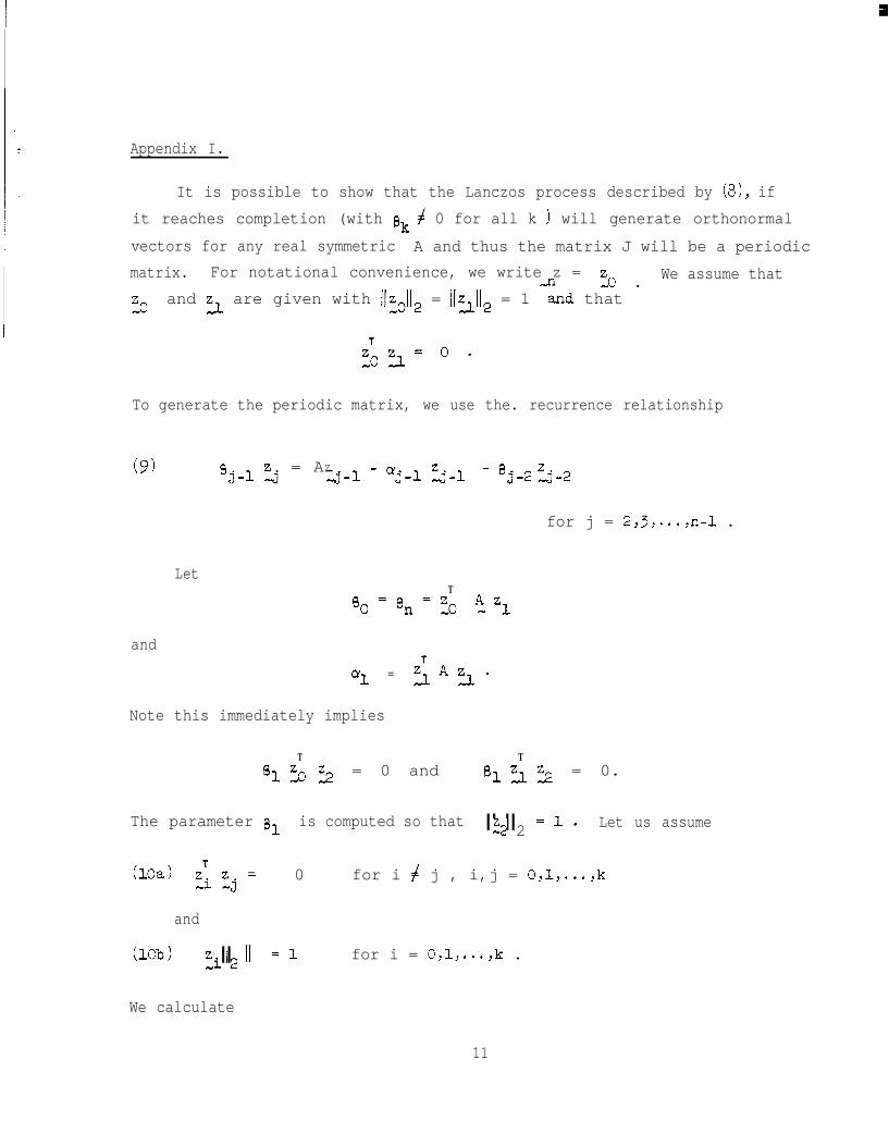
Appendix I.

It is possible to show that the Lanczos process described by (8), if

it reaches completion (with 8, f 0 for all k > will generate orthonormal

vectors for any real symmetric A and thus the matrix J will be a periodic

matrix. For notational convenience, we write z =�,o l

We assume that

EOand Z~ are given with llz_,/2 = l/zJl12 = 1 <nd that

To generate the periodic matrix, we use the. recurrence relationship

(9) ej-l 3 = AZA-1 - aj-l tj-1 - 'j-2 5-2

for j = 2,3,...,n-1 .

LetT

and

a1 = <A3.

Note this immediately implies

T TBlfo 2 = 0 and BIZJ~ = 0.

The parameter Bl is computed so that II IIE2 2=l. Let us assume

(lOa> $fj= 0 for i f j , i,j = O,l,...,k

and

(lob) z2 =lII il for i = O,l,...,k .

We calculate

11

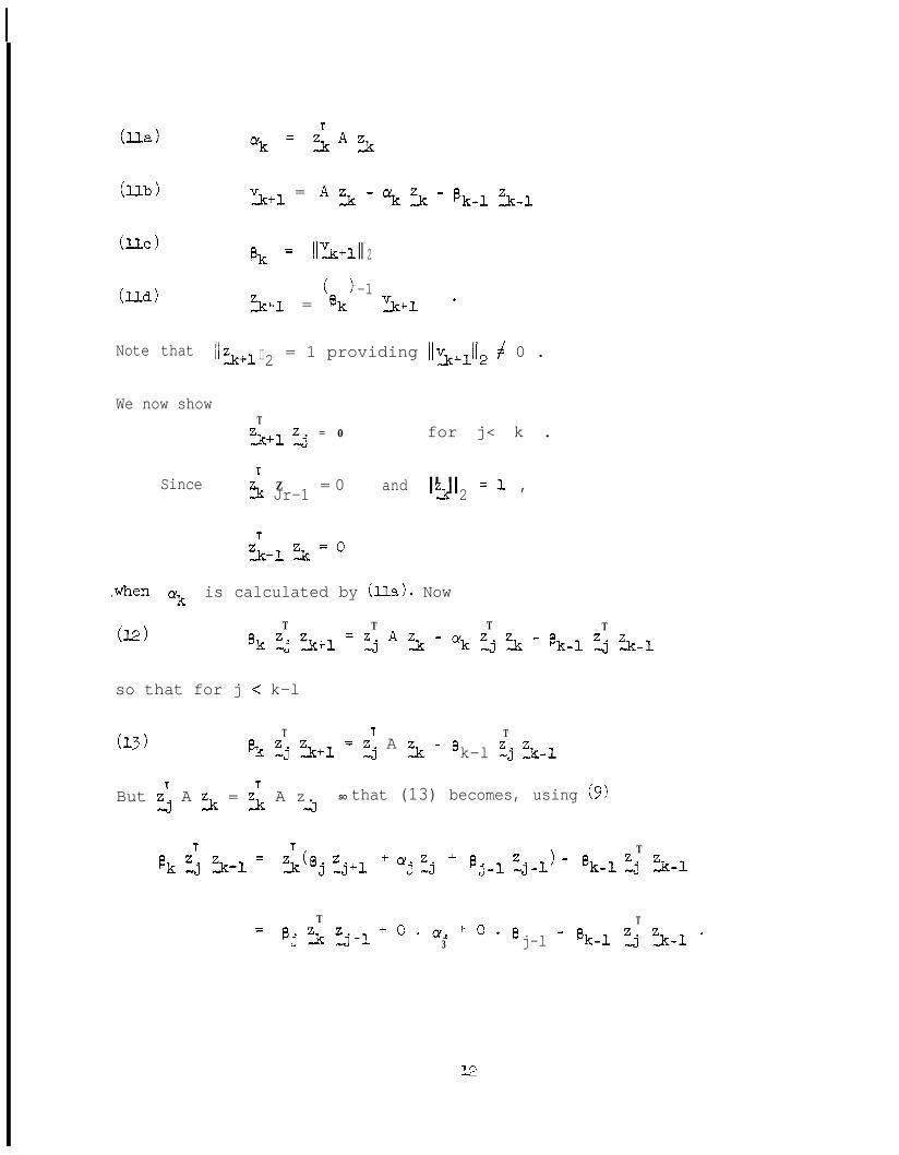
(Ub) Yk+l= AZ&

- cyk 3 - Bk-l s-1

(UC>

(Ud)

8, = II301 II 2( 1 -1

3~1 = @k

Note that II ?k+l 2II = 1 providing /(x+J2 + 0 .

We now show

Since

TzA+l 2 = 0 for j< k .

ic Jr-1Z = 0 and II IIEk 2

=l ,

-when myk is calculated by (Ua). Now

(12)T T T T

Bk zj 'A+1 = "j A '2 - ak "-j 'k - pk-1 "?j 'A-1

so that for j < k-l

(13)T

& zj 'A+1 = JzT A z& -T

0k-l "-j ?k-1

But i. A 5 = z; A z. SO that (13) becomes, using (9)-J

>T

j ",j+l ' aj tj ' B-j-1 fj-1 - *k-l "j L-1

T T=

Bj 'A zmj+l +O.Q.+O.~3 j-l - & 2 'Jr-1 '

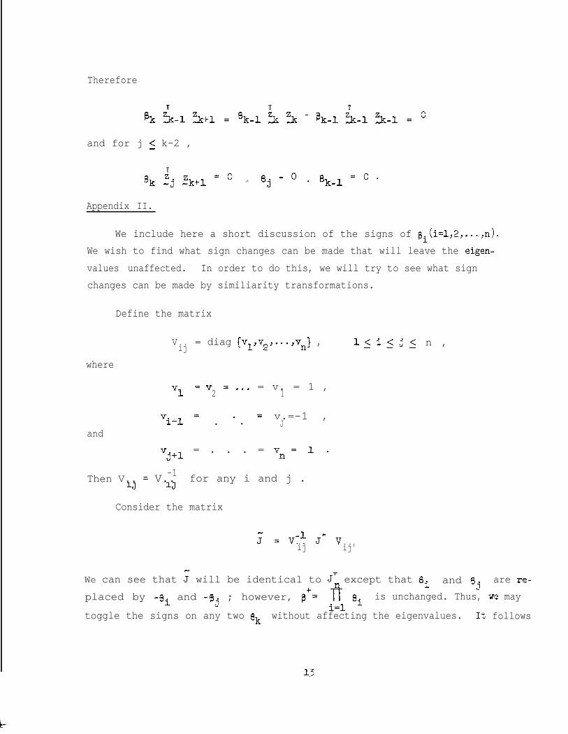
Therefore

P TT T

k 5-1 %I-1 = f&l 'Jr 'A - Bk-1 2-1 '2-1 = '

and for j 5 k-2 ,

T8, zj &+l = O . ej - O l Bk-1 = O �

Appendix II.

We include here a short discussion of the signs of @=1,2,...,n).

We wish to find what sign changes can be made that will leave the eigen-

values unaffected. In order to do this, we will try to see what sign

changes can be made by similiarity transformations.

Define the matrix

Vij

= diag {vl,v2,.*.,vn] , lli,<j,< n ,

where

5 =v2=... = v. = 1 ,

1

vi+l = . ' l

= v.=-1 ,J

and

vj+l = . . . = vn =l.

-1Then V.. = V..

iJ xlfor any i and j .

Consider the matrix

f = V-l J+ Vij ij'

We can see that : will be identical to JT except that pi and B. are re-

placed by ~~~ and -pj ; however, pf= fkJ

is unchanged. Thus, WQ mayi=l Bi

toggle the signs on any two 8k without affecting the eigenvalues. It follows

13

then, that making any even number of sign change will leave the eigenvalues

unaffected.

If we make an odd number of sign changes then by using the above

argument we can see that we get a matrix with the same eigenvalues as J- .

Thus by toggling the signs of the pi we can get only two sets of eigen-

values, those of Jf called {$)~=l and those of J- called (hi)?=1 l

Whichever set we get is determined by how we set the sign of B* .

14