Study on Models for Smart Surveillance through Multi-Camera...
98
Study on Models for Smart Surveillance through Multi-Camera Networks Rahul Raman Department of Computer Science and Engineering National Institute of Technology Rourkela Rourkela – 769 008, India
Transcript of Study on Models for Smart Surveillance through Multi-Camera...
Study on Models for Smart Surveillance
through Multi-Camera Networks
Rahul Raman
Department of Computer Science and Engineering
National Institute of Technology Rourkela
Rourkela – 769 008, India
Study on Models for Smart Surveillance
through Multi-Camera Networks
Dissertation submitted in
November 2013
to the department of
Computer Science and Engineering
of
National Institute of Technology Rourkela
in partial fulfillment of the requirements
for the degree of
M Tech(Research)
by
Rahul Raman
(Roll 611CS101)
under the supervision of
Dr. Pankaj K Sa
Department of Computer Science and Engineering
National Institute of Technology Rourkela
Rourkela – 769 008, India
Computer Science and Engineering
National Institute of Technology Rourkela
Rourkela-769 008, India. www.nitrkl.ac.in
Dr. Pankaj K Sa
Assistant Professor
Nov 07, 2013
Certificate
This is to certify that the work in the thesis entitled Study on Models for Smart
Surveillance through Multi-Camera Networks by Rahul Raman , is a
record of an original research work carried out by him under my supervision and
guidance in partial fulfilment of the requirements for the award of the degree of
Master of Technology (Research) in Computer Science and Engineering. Neither
this thesis nor any part of it has been submitted for any degree or academic award
elsewhere.
Pankaj K Sa

Acknowledgment
I pay my sincere thanks to Dr. Pankaj K Sa for believing in my abilities to
work in the challenging domain of visual surveillance and for his efforts towards
transforming my novice ideas into research thesis, to Prof. Banshidhar Majhi for
providing constant motivation and support, to Sambit Bakshi for always backing
me with his all round abilities and to my lab mates for creating together a healthy
work culture.
Support of my parents and loved ones were always there, when I stayed away from
them. I thank God for blessing with such family and friends in my life.
I finally acknowledge the positive energy received in the aroma of my institute that
kept me striving throughout.
Rahul Raman
Abstract
With ever changing world, visual surveillance once a distinctive issue has now became
an indispensable component of surveillance system and multi-camera network are
the most suited way to achieve them. Even though multi-camera network has
manifold advantage over single camera based surveillance, still it adds overheads
towards processing, memory requirement, energy consumption, installation costs
and complex handling of the system.
This thesis explores different challenges in the domain of multi-camera network
and surveys the issue of camera calibration and localization. The survey presents an
in-depth study of evolution of camera localization over the time. This study helps in
realizing the complexity as well as necessity of camera localization in multi-camera
network.
This thesis proposes smart visual surveillance model that study phases of
multi-camera network development model and proposes algorithms at the level of
camera placement and camera control. It proposes camera placement technique
for gait pattern recognition and a smart camera control governed by occlusion
determination algorithm that leads to reducing the number of active camera thus
eradicating many overheads yet not compromising with the standards of surveillance.
The proposed camera placement technique has been tested over self-acquired
data from corridor of Vikram Sarabhai Hall of Residence, NIT Rourkela. The
proposed algorithm provides probable places for camera placement in terms of 3D
plot depicting the suitability of camera placement for gait pattern recognition.
The control flow between cameras is governed by a three step algorithm that
works on direction and apparent speed estimation of moving subjects to determine
the chances of occlusion between them. The algorithms are tested over self-acquired
as well as existing gait database CASIA Dataset A for direction determination as
well as occlusion estimation.
Keywords: Visual surveillance, Multi-camera network, Multi-camera localization, Gait
biometric and camera placement, Height based identification, Perspective view analysis, Occlusion
determination algorithm, Motion direction estimation.
Contents
Certificate ii
Acknowledgement iii
Abstract iv
List of Figures vii
List of Tables ix
1 Introduction 1
1.1 Research Challenges in MCN . . . . . . . . . . . . . . . . . . . . . . 2
1.2 Literature Survey . . . . . . . . . . . . . . . . . . . . . . . . . . . . . 7
1.2.1 Camera Localization and Calibration . . . . . . . . . . . . . . 7
1.2.2 Camera Placement for Gait Based Identification . . . . . . . . 25
1.2.3 Camera Control for Occlusion Avoidance . . . . . . . . . . . . 30
1.3 Thesis Organization . . . . . . . . . . . . . . . . . . . . . . . . . . . . 32
2 Study on Efficient Camera Placement Techniques 33
2.1 Gait Biometric . . . . . . . . . . . . . . . . . . . . . . . . . . . . . . 34
2.2 Proposed Model . . . . . . . . . . . . . . . . . . . . . . . . . . . . . . 36
2.2.1 Locus Tracking of Subjects’ Movement . . . . . . . . . . . . . 38
2.2.2 Direction Vector Calculation . . . . . . . . . . . . . . . . . . . 39
2.2.3 Path-band Estimation . . . . . . . . . . . . . . . . . . . . . . 40
v
2.2.4 Finding Efficient Camera Placement . . . . . . . . . . . . . . 41
2.2.5 Localization and Working of Camera Network . . . . . . . . 42
2.3 Experiment . . . . . . . . . . . . . . . . . . . . . . . . . . . . . . . . 43
2.4 Concluding Remarks . . . . . . . . . . . . . . . . . . . . . . . . . . 46
3 Study on Smart Camera Control 48
3.1 Database Used . . . . . . . . . . . . . . . . . . . . . . . . . . . . . . 50
3.2 Motion analysis . . . . . . . . . . . . . . . . . . . . . . . . . . . . . . 51
3.2.1 Determination of Direction of Motion . . . . . . . . . . . . . . 51
3.2.2 Apparent Speed Determination . . . . . . . . . . . . . . . . . 62
3.3 Occlusion Determination . . . . . . . . . . . . . . . . . . . . . . . . . 64
3.3.1 Lookup table generation . . . . . . . . . . . . . . . . . . . . . 65
3.3.2 Time and Location of Occlusion Calculation . . . . . . . . . . 67
3.4 Mitigation of Occlusion . . . . . . . . . . . . . . . . . . . . . . . . . . 71
3.5 Results . . . . . . . . . . . . . . . . . . . . . . . . . . . . . . . . . . . 71
3.6 Concluding Remarks . . . . . . . . . . . . . . . . . . . . . . . . . . . 73
4 Conclusion 75
Bibliography 78
Dissemination 87
Vitae 88
vi
List of Figures
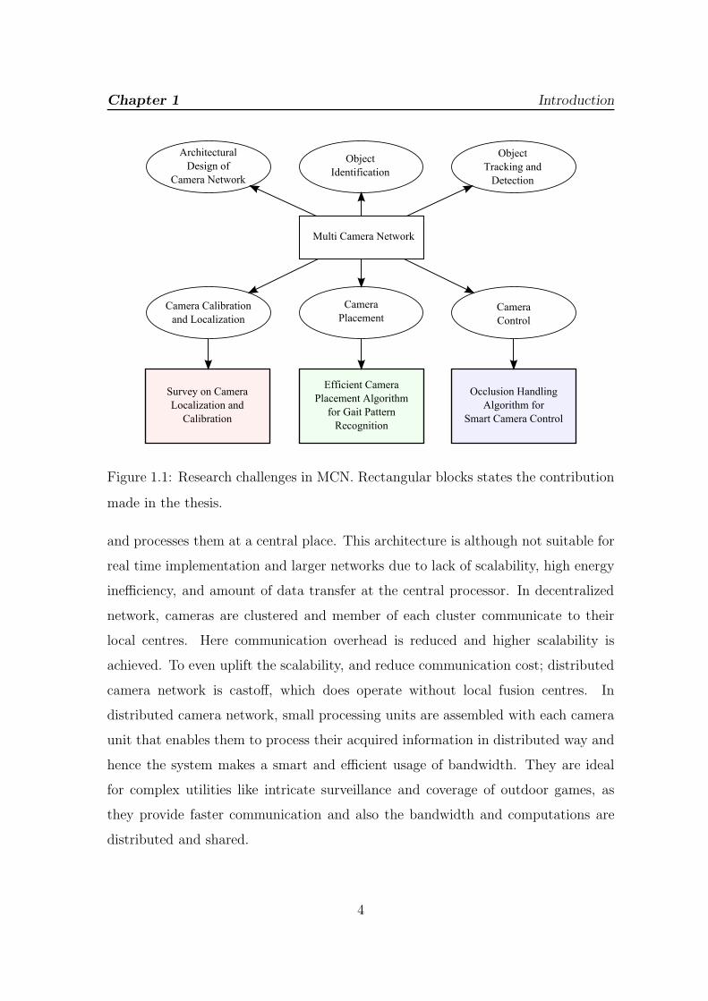
1.1 Research challenges in MCN. Rectangular blocks states the
contribution made in the thesis. . . . . . . . . . . . . . . . . . . . . . 4
1.2 Images of Different camera network. . . . . . . . . . . . . . . . . . . 6
1.3 Analogy between formation of sensor connectivity graph and vision
graph . . . . . . . . . . . . . . . . . . . . . . . . . . . . . . . . . . . . 11
1.4 Formation of epipolar geometry . . . . . . . . . . . . . . . . . . . . . 13
1.5 Simultaneous localization techniques . . . . . . . . . . . . . . . . . . 16
2.1 A complete gait cycle . . . . . . . . . . . . . . . . . . . . . . . . . . . 35
2.2 Change in width of bounding box of moving object with different
camera placement angle . . . . . . . . . . . . . . . . . . . . . . . . . 38
2.3 Loci of different subjects tracked by the overhead-camera . . . . . . 39
2.4 Inference of angles from discrete pixel patterns in 8× 8 grid . . . . . 40
2.5 (a) Grid indicating unique direction of movement, (b) chaos region,
(c) grid with no locus . . . . . . . . . . . . . . . . . . . . . . . . . . 41
2.6 Finding efficient camera placement . . . . . . . . . . . . . . . . . . . 42
2.7 Corridor sequence . . . . . . . . . . . . . . . . . . . . . . . . . . . . . 43
2.8 Finding trace of the subjects by optical flow . . . . . . . . . . . . . . 44
2.9 Plotting traces over grid-map from captured images by homography . 45
2.10 Sample grid and histogram for orientation of movements in the grid . 45
2.11 3D mesh plot where two of the humps depicting probable places for
camera placement . . . . . . . . . . . . . . . . . . . . . . . . . . . . . 47
vii
3.1 Proposed camera control model governed by occlusion determination
algorithm . . . . . . . . . . . . . . . . . . . . . . . . . . . . . . . . . 49
3.2 Discrete directions of motion with respect to camera . . . . . . . . . . 52
3.3 Pattern change in the dimension of subject . . . . . . . . . . . . . . . 53
3.4 Variation of height with respect to frame number for four different
direction of subject’s motion . . . . . . . . . . . . . . . . . . . . . . . 54
3.5 Plot of width for different direction . . . . . . . . . . . . . . . . . . . 54
3.6 Frame rectification and unwanted blob removal . . . . . . . . . . . . 56
3.7 Morphological operations and tracking of subject . . . . . . . . . . . 57
3.8 Envelop over the plot . . . . . . . . . . . . . . . . . . . . . . . . . . 58
3.9 Detection and removal of soft extremas . . . . . . . . . . . . . . . . . 58
3.10 Envelop and average line drawn based on envelop . . . . . . . . . . . 61
3.11 Distance invariant direction of motion estimation through phase . . . 61
3.12 Direction estimation result based on height of the subject . . . . . . 63
3.13 Direction estimation result based on width of the subject . . . . . . 63
3.14 Test cases depicting occlusion over CASIA Dataset A . . . . . . . . . 72
3.15 Test cases depicting occlusion and non occlusion . . . . . . . . . . . . 73
viii
List of Tables
1.1 Different approaches to solve point correspondence problem . . . . . . 14
1.2 Review of related researches on multi-camera localization . . . . . . . 19
1.3 Task specific optimal camera placement . . . . . . . . . . . . . . . . . 29
3.1 Matrix for direction based occlusion probability estimation . . . . . . 68
3.2 Matrix for speed based occlusion determination with directions
(Di, Dj)|(i, j) ∈ {2, 3, 4} . . . . . . . . . . . . . . . . . . . . . . . . . 68
3.3 Matrix for speed based occlusion determination with directions
(Di, Dj)|(i, j) ∈ {6, 7, 8} . . . . . . . . . . . . . . . . . . . . . . . . . 68
ix
Chapter 1
Introduction
Vision is an ideal sensing mechanism and since the evolution of cameras, image
processing are perceived as solution of many complex real world problems.
Processing of images first require that they should be represented in proper format
for which the one dimensional signal has up-scaled its dimension to image and
thereby increasing its processing complexity. The complexity has further uplifted
in video processing with an additional dimension. Complexity in video processing
is also compounded by inter frame and intra frame processing. The wide scope of
image and video processing find its implementation in almost every walk of life, be it
medicine or engineering, space or mining, agriculture or weather forecast, image and
video processing are omnipresent. In recent days, visual surveillance has became
an important issue that has been greatly deciphered through video processing. An
important application of video processing is visual surveillance. As the demand of
sophisticated visual surveillance mechanism prevailed, so is the research over the
constraint of earlier surveillance systems are much discussed and it resulted in a
paradigm shift toward visual surveillance through multi-camera network.
Multi camera network (MCN) overcomes many limitations of single camera
surveillance systems like restricted field of view, no options for best view synthesis,
partial and full occlusion of subject during tracking. Multi-camera based surveillance
although considered as the solution to overcome these limitations of single camera
1
Chapter 1 Introduction
based surveillance but are more complex. They require higher installation cost and
complex algorithm for handling as well. This thesis concentrates on understanding
research challenges in multi-camera based visual surveillance and presents survey,
proposals, experiments and results towards development of smart multi-camera
network based surveillance system.
Next section discusses various research challenges in MCN. Some of the research
challenges are extensively studied and discussed in Section 1.2. The organization of
the thesis is presented in the last section.
1.1 Research Challenges in MCN
As the demand for fool-proof tracking algorithm prevailed, so is the paradigm shifted
from single to multi-camera network model. These systems are more useful for
tracking in crowded places and highly protected areas. This can be equipped with
a variety of cameras and distributed processors to even amend the functionality of
tracking. Here are a few reasons that made the mode of surveillance to change from
single camera to MCN:
(i) Growing importance of visual surveillance
(ii) Coverage area becoming larger and more complex.
(iii) Occurrences of occlusion can be avoided.
(iv) Best view synthesis algorithms can be applied when multiple views of the same
scene are available.
(v) Decreased cost of sensors and other hardware in recent years.
(vi) Can be made smart and interactive with variety of cameras, distributed
processors, and state of the art software.
A multi-camera system can avoid occlusion and can provide robust tracking but
are not as simple and energy-efficient as single camera systems. Although a camera
2
Chapter 1 Introduction
system installed in master-slave mode [9], has the energy efficiency but the entire
region under coverage should come under master camera’s view. Towards making
the multi-camera model efficient, few other works have also been proposed. Kulkarni
et al. have proposed an approach for efficient use of multiple cameras by devising
multi-tier camera network called SensEye [1, 2]. This approach is energy efficient
although it has a complex hardware architecture and diverse software requirement.
Even though surveillance through MCN has many advantages over single camera
system, yet it has some bottlenecks that restrict the use of MCN to serve only some
vital requirements. Some of the limitations are:
(i) Need additional processing.
(ii) Require extra memory.
(iii) Consume superfluous energy.
(iv) Have higher installation cost.
(v) Demand complex handling and implementation.
(vi) Obligate localization and calibration.
(vii) Need suitable camera placement.
Some of the key research challenges are identified as in Figure 1.1 and are briefly
discussed here.
Camera and Camera Network When many cameras are allied via a network,
so that they can interact among them, they form a camera network. Deciding
the type of camera network is one of the major issue in MCN. Based on
inter-sensor communication, a camera network may follow centralized, decentralized,
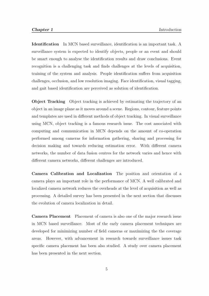
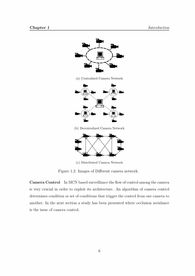
or distributed architecture for interconnection. Figure 1.2 shows the diagrammatic
representation of centralized, decentralized, and distributed camera network. In
centralized network, a single node receives raw information from all the cameras
3
Chapter 1 Introduction
Multi Camera Network
Architectural
Design of
Camera Network
Object
Identification
Object
Tracking and
Detection
Camera Calibration
and Localization
Camera
PlacementCamera
Control
Survey on Camera
Localization and
Calibration
Efficient Camera
Placement Algorithm
for Gait Pattern
Recognition
Occlusion Handling
Algorithm for
Smart Camera Control
Figure 1.1: Research challenges in MCN. Rectangular blocks states the contribution
made in the thesis.
and processes them at a central place. This architecture is although not suitable for
real time implementation and larger networks due to lack of scalability, high energy
inefficiency, and amount of data transfer at the central processor. In decentralized
network, cameras are clustered and member of each cluster communicate to their
local centres. Here communication overhead is reduced and higher scalability is
achieved. To even uplift the scalability, and reduce communication cost; distributed
camera network is castoff, which does operate without local fusion centres. In
distributed camera network, small processing units are assembled with each camera
unit that enables them to process their acquired information in distributed way and
hence the system makes a smart and efficient usage of bandwidth. They are ideal
for complex utilities like intricate surveillance and coverage of outdoor games, as
they provide faster communication and also the bandwidth and computations are
distributed and shared.
4
Chapter 1 Introduction
Identification In MCN based surveillance, identification is an important task. A
surveillance system is expected to identify objects, people or an event and should
be smart enough to analyse the identification results and draw conclusions. Event
recognition is a challenging task and finds challenges at the levels of acquisition,
training of the system and analysis. People identification suffers from acquisition
challenges, occlusion, and low resolution imaging. Face identification, visual tagging,
and gait based identification are perceived as solution of identification.
Object Tracking Object tracking is achieved by estimating the trajectory of an
object in an image plane as it moves around a scene. Regions, contour, feature points
and templates are used in different methods of object tracking. In visual surveillance
using MCN, object tracking is a famous research issue. The cost associated with
computing and communication in MCN depends on the amount of co-operation
performed among cameras for information gathering, sharing and processing for
decision making and towards reducing estimation error. With different camera
networks, the number of data fusion centres for the network varies and hence with
different camera networks, different challenges are introduced.
Camera Calibration and Localization The position and orientation of a
camera plays an important role in the performance of MCN. A well calibrated and
localized camera network reduces the overheads at the level of acquisition as well as
processing. A detailed survey has been presented in the next section that discusses
the evolution of camera localization in detail.
Camera Placement Placement of camera is also one of the major research issue
in MCN based surveillance. Most of the early camera placement techniques are
developed for minimizing number of field cameras or maximizing the the coverage
areas. However, with advancement in research towards surveillance issues task
specific camera placement has been also studied. A study over camera placement
has been presented in the next section.
5
Chapter 1 Introduction
(a) Centralized Camera Network
(b) Decentralized Camera Network
(c) Distributed Camera Network
Figure 1.2: Images of Different camera network.
Camera Control In MCN based surveillance the flow of control among the camera
is very crucial in order to exploit its architecture. An algorithm of camera control
determines condition or set of conditions that trigger the control from one camera to
another. In the next section a study has been presented where occlusion avoidance
is the issue of camera control.
6

Chapter 1 Introduction
1.2 Literature Survey
In order to understand the challenges identified at different levels of MCN
based surveillance, study has been performed on different domain of MCN based
surveillance.
Section 1.2.1 presents an extensive survey on camera calibration and localization
that portrays the diversity in the approach of achieving camera localization. The
survey explores evolution of camera localization, different approaches of camera
localizations and comparison among different localization methods. Section 1.2.2
highlights the need of camera placement in MCN based surveillance. Task specific
camera placement has been explored for different task and a study on camera
placement with gait pattern recognition as test case has been presented. Section
1.2.3 presents a study over camera control in MCN for occlusion avoidance. Various
approaches where camera control is governed by occlusion avoidance mechanism are
discussed in the context of single camera as well as multi-camera based surveillance.
1.2.1 Camera Localization and Calibration
Location of camera in an MCN plays important role in its performance. These
locations are given by certain number of parameters, which define its position
in global frame. These parameters help in achieving view interpretation and
multi-camera communication in MCN and are called camera calibration parameters.
Camera calibration parameters include a set of intrinsic constraints i.e. focal range,
principal point, scale factors, and lens distortion and a set of extrinsic calibration
parameters like camera position and its orientation. Intrinsic calibration parameters
are very much dependent on camera make and are valuable in deciding the suitability
of camera for a typical purpose. On the other hand, extrinsic parameter give the
camera pose (position and orientation) and decides the position of camera as well
as the subject in global frame. These extrinsic calibrations in a network of multiple
cameras are also called as camera localization. This section presents an in-depth
7
Chapter 1 Introduction
study on camera localization, exploring the advent of localization techniques with
gradually increasing complexity of MCN.
For the operation of multi-camera network, information of location of other
cameras is the pre-requisite for each camera. This process of establishing a relation
among the camera coordinates is termed as camera localization. Manual localization
methods of multi-camera network failed to handle large number of cameras in
network. Automation of the localization process started gaining importance to
ascertain accuracy and real-time localization. One of the primitive automated
solutions to localization has been through GPS [3]. However, it has failed mostly due
to the poor resolution. Efforts have also been made towards developing localization
algorithms on single processor after collecting images from all the networked cameras
in a single room [4,5]. But in practical scenario, large number of cameras producing
high volume of images and video data makes the analysis time-consuming on single
processor. The subsequent attempts of developing localization algorithms deploy
more than one processor concurrently to achieve real-time localization. These
approaches differ in variety of coverage areas, assumptions made on deployment
of the nodes, and the way sensors work [6].
Pioneer works
Early automated localization techniques for static sensors, viz. non-camera equipped
networks have used ultra-sound, radio, or acoustic signals [7]. Likewise, moving
sensors like robots have exploited LED based techniques for their localization.
However all the methods proposed have been based on heuristic approaches and
lagged theoretical foundation of network localization until Aspnes et al. [8] have
identified specific problems and solved them theoretically. This work, motivated by
previous work of Eren et al. [9], have attempted to give systematic answer to the
following questions:
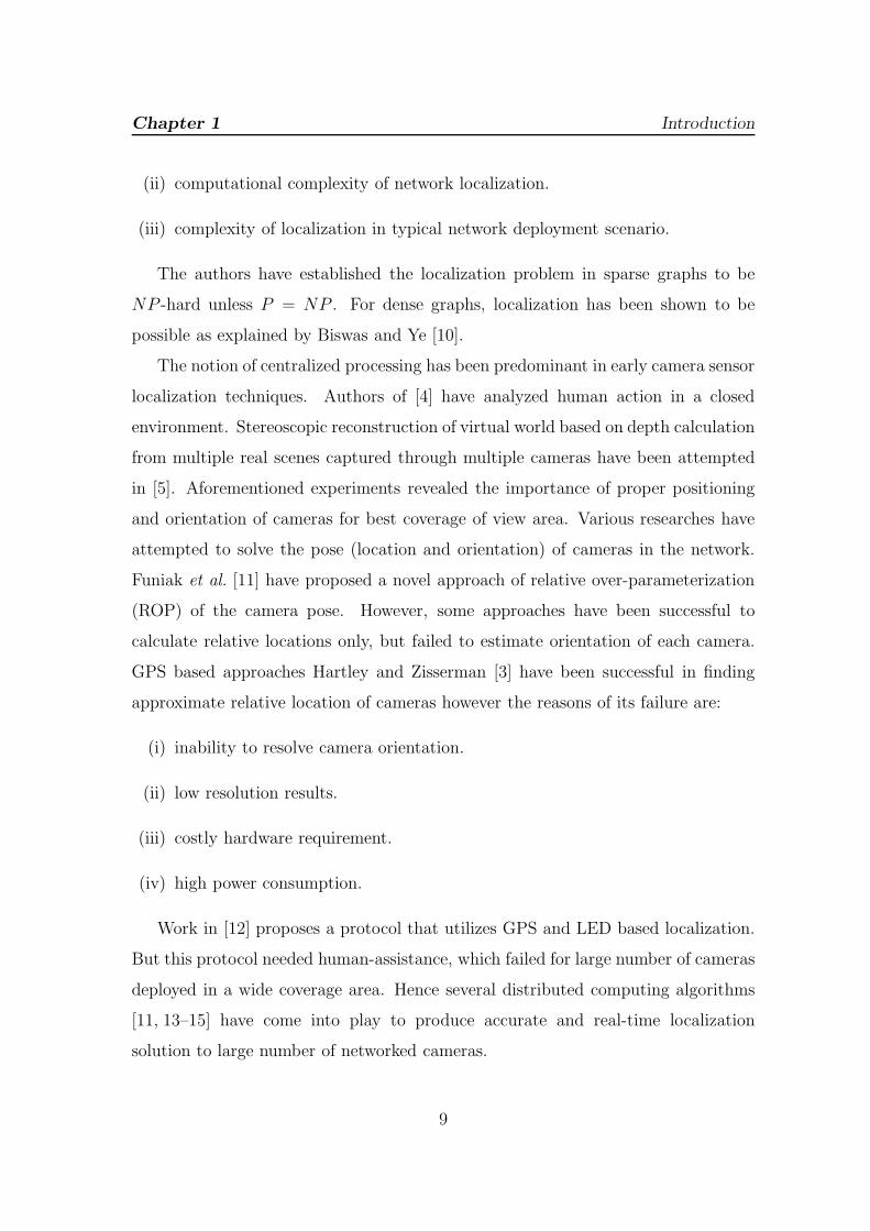
(i) conditions for unique network localizability.
8
Chapter 1 Introduction
(ii) computational complexity of network localization.
(iii) complexity of localization in typical network deployment scenario.
The authors have established the localization problem in sparse graphs to be
NP -hard unless P = NP . For dense graphs, localization has been shown to be
possible as explained by Biswas and Ye [10].
The notion of centralized processing has been predominant in early camera sensor
localization techniques. Authors of [4] have analyzed human action in a closed
environment. Stereoscopic reconstruction of virtual world based on depth calculation
from multiple real scenes captured through multiple cameras have been attempted
in [5]. Aforementioned experiments revealed the importance of proper positioning
and orientation of cameras for best coverage of view area. Various researches have
attempted to solve the pose (location and orientation) of cameras in the network.
Funiak et al. [11] have proposed a novel approach of relative over-parameterization
(ROP) of the camera pose. However, some approaches have been successful to
calculate relative locations only, but failed to estimate orientation of each camera.
GPS based approaches Hartley and Zisserman [3] have been successful in finding
approximate relative location of cameras however the reasons of its failure are:
(i) inability to resolve camera orientation.
(ii) low resolution results.
(iii) costly hardware requirement.
(iv) high power consumption.
Work in [12] proposes a protocol that utilizes GPS and LED based localization.
But this protocol needed human-assistance, which failed for large number of cameras
deployed in a wide coverage area. Hence several distributed computing algorithms
[11, 13–15] have come into play to produce accurate and real-time localization
solution to large number of networked cameras.
9
Chapter 1 Introduction
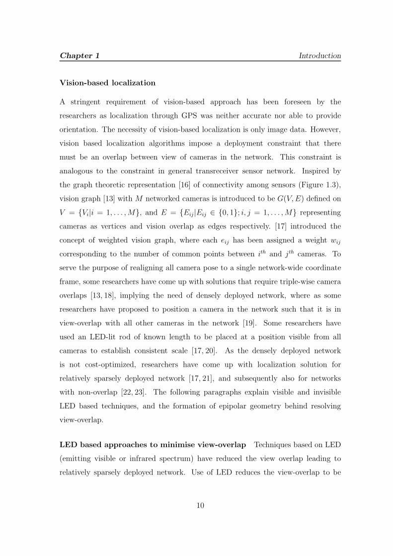
Vision-based localization
A stringent requirement of vision-based approach has been foreseen by the
researchers as localization through GPS was neither accurate nor able to provide
orientation. The necessity of vision-based localization is only image data. However,
vision based localization algorithms impose a deployment constraint that there
must be an overlap between view of cameras in the network. This constraint is
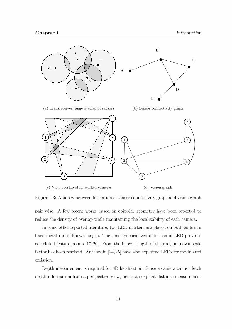
analogous to the constraint in general transreceiver sensor network. Inspired by
the graph theoretic representation [16] of connectivity among sensors (Figure 1.3),
vision graph [13] with M networked cameras is introduced to be G(V,E) defined on
V = {Vi|i = 1, . . . ,M}, and E = {Eij |Eij ∈ {0, 1}; i, j = 1, . . . ,M} representing
cameras as vertices and vision overlap as edges respectively. [17] introduced the
concept of weighted vision graph, where each eij has been assigned a weight wij
corresponding to the number of common points between ith and jth cameras. To
serve the purpose of realigning all camera pose to a single network-wide coordinate
frame, some researchers have come up with solutions that require triple-wise camera
overlaps [13, 18], implying the need of densely deployed network, where as some
researchers have proposed to position a camera in the network such that it is in
view-overlap with all other cameras in the network [19]. Some researchers have
used an LED-lit rod of known length to be placed at a position visible from all
cameras to establish consistent scale [17, 20]. As the densely deployed network
is not cost-optimized, researchers have come up with localization solution for
relatively sparsely deployed network [17, 21], and subsequently also for networks
with non-overlap [22, 23]. The following paragraphs explain visible and invisible
LED based techniques, and the formation of epipolar geometry behind resolving
view-overlap.
LED based approaches to minimise view-overlap Techniques based on LED
(emitting visible or infrared spectrum) have reduced the view overlap leading to
relatively sparsely deployed network. Use of LED reduces the view-overlap to be
10
Chapter 1 Introduction
(a) Transreceiver range overlap of sensors (b) Sensor connectivity graph
(c) View overlap of networked cameras (d) Vision graph
Figure 1.3: Analogy between formation of sensor connectivity graph and vision graph
pair wise. A few recent works based on epipolar geometry have been reported to
reduce the density of overlap while maintaining the localizability of each camera.
In some other reported literature, two LED markers are placed on both ends of a
fixed metal rod of known length. The time synchronized detection of LED provides
correlated feature points [17,20]. From the known length of the rod, unknown scale
factor has been resolved. Authors in [24,25] have also exploited LEDs for modulated
emission.
Depth measurement is required for 3D localization. Since a camera cannot fetch
depth information from a perspective view, hence an explicit distance measurement
11
Chapter 1 Introduction
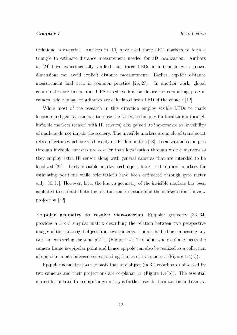
technique is essential. Authors in [19] have used three LED markers to form a
triangle to estimate distance measurement needed for 3D localization. Authors
in [24] have experimentally verified that three LEDs in a triangle with known
dimensions can avoid explicit distance measurement. Earlier, explicit distance
measurement had been in common practice [26, 27]. In another work, global
co-ordinates are taken from GPS-based calibration device for computing pose of
camera, while image coordinates are calculated from LED of the camera [12].
While most of the research in this direction employ visible LEDs to mark
location and general cameras to sense the LEDs, techniques for localization through
invisible markers (sensed with IR sensors) also gained its importance as invisibility
of markers do not impair the scenery. The invisible markers are made of translucent
retro-reflectors which are visible only in IR illumination [28]. Localization techniques
through invisible markers are costlier than localization through visible markers as
they employ extra IR sensor along with general cameras that are intended to be
localized [29]. Early invisible marker techniques have used infrared markers for
estimating positions while orientations have been estimated through gyro meter
only [30, 31]. However, later the known geometry of the invisible markers has been
exploited to estimate both the position and orientation of the markers from its view
projection [32].
Epipolar geometry to resolve view-overlap Epipolar geometry [33, 34]
provides a 3 × 3 singular matrix describing the relation between two perspective
images of the same rigid object from two cameras. Epipole is the line connecting any
two cameras seeing the same object (Figure 1.4). The point where epipole meets the
camera frame is epipolar point and hence epipole can also be realized as a collection
of epipolar points between corresponding frames of two cameras (Figure 1.4(a)).
Epipolar geometry has the basis that any object (in 3D coordinate) observed by
two cameras and their projections are co-planar [3] (Figure 1.4(b)). The essential
matrix formulated from epipolar geometry is further used for localization and camera
12
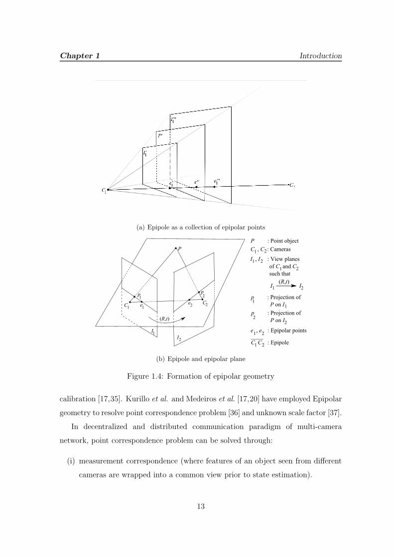
Chapter 1 Introduction
(a) Epipole as a collection of epipolar points
(b) Epipole and epipolar plane
Figure 1.4: Formation of epipolar geometry
calibration [17,35]. Kurillo et al. and Medeiros et al. [17,20] have employed Epipolar
geometry to resolve point correspondence problem [36] and unknown scale factor [37].
In decentralized and distributed communication paradigm of multi-camera
network, point correspondence problem can be solved through:
(i) measurement correspondence (where features of an object seen from different
cameras are wrapped into a common view prior to state estimation).
13
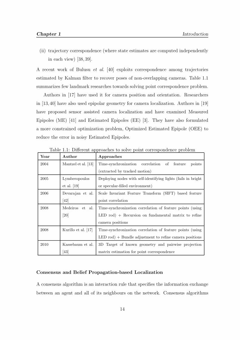
Chapter 1 Introduction
(ii) trajectory correspondence (where state estimates are computed independently
in each view) [38, 39].
A recent work of Bulusu et al. [40] exploits correspondence among trajectories
estimated by Kalman filter to recover poses of non-overlapping cameras. Table 1.1
summarizes few landmark researches towards solving point correspondence problem.
Authors in [17] have used it for camera position and orientation. Researchers
in [13,40] have also used epipolar geometry for camera localization. Authors in [19]
have proposed sensor assisted camera localization and have examined Measured
Epipoles (ME) [41] and Estimated Epipoles (EE) [3]. They have also formulated
a more constrained optimization problem, Optimized Estimated Epipole (OEE) to
reduce the error in noisy Estimated Epipoles.
Table 1.1: Different approaches to solve point correspondence problem
Year Author Approaches
2004 Mantzel et al. [13] Time-synchronization correlation of feature points
(extracted by tracked motion)
2005 Lymberopoulos
et al. [19]
Deploying nodes with self-identifying lights (fails in bright
or specular-filled environment)
2006 Devarajan et al.
[42]
Scale Invariant Feature Transform (SIFT) based feature
point correlation
2008 Medeiros et al.
[20]
Time-synchronization correlation of feature points (using
LED rod) + Recursion on fundamental matrix to refine
camera positions
2008 Kurillo et al. [17] Time-synchronization correlation of feature points (using
LED rod) + Bundle adjustment to refine camera positions
2010 Kassebaum et al.
[43]
3D Target of known geometry and pairwise projection
matrix estimation for point correspondence
Consensus and Belief Propagation-based Localization
A consensus algorithm is an interaction rule that specifies the information exchange
between an agent and all of its neighbours on the network. Consensus algorithms
14
Chapter 1 Introduction
are used in many situations, viz. distributed formation control, synchronization,
rendezvous in space, distributed fusion in sensor, flocking theory [44].
Consensus algorithms are used for getting global pose of a camera in a network,
and have been used for localization with range measurements [45, 46]. Tron and
Vidal [47] have generalized the consensus algorithm for estimating pose of each node
from noisy and inconsistent measurements.
On contrary to this, notion of belief propagation have also been proposed for
establishing localization [14]. Belief propagation is a message passing technique
for graphical network model which have been applied for scene estimation, shape
finding, image segmentation, restoration, and tracking [48–52]. Belief propagation
has originally been developed for trees. When applied for graphs with cycles,
inferences (belief) might not converge, and even if convergence occurs, density is not
guaranteed [53, 54]. The non-convergent form of belief propagation (Loopy Belief
Propagation (LBP)) [53] is used in sharing localization parameters in multi-camera
localization.
Authors in [55] have presented a more robust algorithm than belief propagation
in several aspects. This approach has been extended by researchers in [56] for
localization of robot in multi-camera scenario (SLAM: Simultaneous Localization
And Mapping) [57] where a robot observes all the landmarks and estimates its
location and position of the landmarks. A similar concept has been proposed by
Funiak et al. [11] for camera localization (SLAT: Simultaneous Localization And
Tracking), where the camera replaces the landmarks and robot is replaced by a
moving object. Robot observes the landmarks in SLAM (Figure 1.5(a)), whereas
cameras observe the object in SLAT (Figure 1.5(b)). Funiak et al. [11] has also
proposed Relative Over-Parameterization (ROP) to represent the distribution in
SLAT problem using single Gaussian.
There had been efforts to find the trajectory of object and pose of camera
simultaneously [11, 58]. In particular, Rekleitis et al.. have addressed the issue of
15
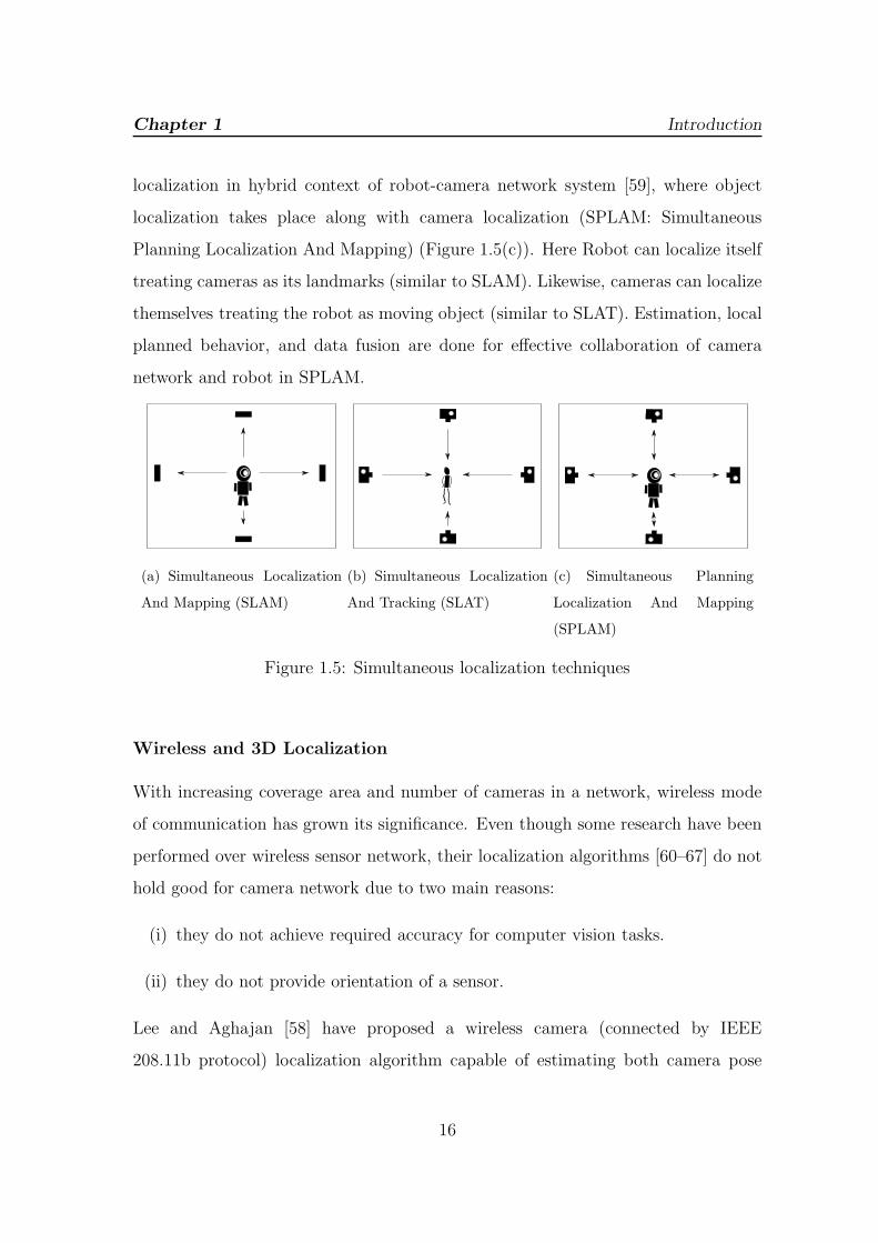
Chapter 1 Introduction
localization in hybrid context of robot-camera network system [59], where object
localization takes place along with camera localization (SPLAM: Simultaneous
Planning Localization And Mapping) (Figure 1.5(c)). Here Robot can localize itself
treating cameras as its landmarks (similar to SLAM). Likewise, cameras can localize
themselves treating the robot as moving object (similar to SLAT). Estimation, local
planned behavior, and data fusion are done for effective collaboration of camera
network and robot in SPLAM.
(a) Simultaneous Localization
And Mapping (SLAM)
(b) Simultaneous Localization
And Tracking (SLAT)
(c) Simultaneous Planning
Localization And Mapping
(SPLAM)
Figure 1.5: Simultaneous localization techniques
Wireless and 3D Localization
With increasing coverage area and number of cameras in a network, wireless mode
of communication has grown its significance. Even though some research have been
performed over wireless sensor network, their localization algorithms [60–67] do not
hold good for camera network due to two main reasons:
(i) they do not achieve required accuracy for computer vision tasks.
(ii) they do not provide orientation of a sensor.
Lee and Aghajan [58] have proposed a wireless camera (connected by IEEE
208.11b protocol) localization algorithm capable of estimating both camera pose
16

Chapter 1 Introduction
and trajectory of the object. This work has been experimented in 2D plane with
only five cameras, while authors in [20] have proposed four different localization
approaches simulated in a 20 × 20 × 20m3 3D region with 50 randomly placed
cameras. The system developed in [20] can perform in fully-distributed scenario,
and does not require anchor-nodes. This approach employs feature-based object
trajectory estimation, and hence performs depending on robustness of the used
feature-extraction algorithm.
3D image reconstruction has remained an active research area in computer vision
for many years. Tomassi and Kanade [68] have used matrix factorization as a way
for reconstructing a scene, as well as to estimate camera parameters and frame point
localization. This work has employed orthographic projection whereas authors in [69]
have used perspective projection to serve the same. Sturm and Triggs [27] has also
proposed more complete solution for measuring camera depth. Rahimi et al. [23]
have pre-computed the homographies between image plane of each camera, and a
common ground plane leading to 3D localization of cameras.
Lymberopoulos et al. [19] have proposed an algorithm that combines a sparse
set of distance measurements with image information of each camera. It uses three
LED triangles of known geometry for depth measurement. Tron and Vidal [47] have
taken the work to distributed level by applying consensus algorithm and thereby
enhancing the work of [6] and have generalized it from 2D to 3D.
Latest works on 3D camera localization include the work of [43]. Kassebaum et
al. [43] have used 3D target. This is similar to the 2D targets like checker boards
used earlier in [70, 71]. The advantage of 3D target is that in one frame it provides
all the feature points needed by a camera to determine its position and orientation
relative to the target. On detected feature points, DLT [72] is used to estimate
projection matrix. The algorithm reduces the cost of feature point detection, number
of overlaps and eliminates the unknown scale factor problem. Kassebaum et al. [43]
have experimented with error less than 1in when 3D target feature point fills only
17
Chapter 1 Introduction
2.9% of the frame.
Concluding Remarks
Networked communication in early days used to exploit sound, radio and other
acoustic signals for localization of static sensors. However, with the development
of multi-camera network, it gradually became stringent to localize the nodes for
initialization of a camera-network. There are several method devised depending
on different types of coverage area, different strength of cameras in network,
different types of camera used, and different purpose of the camera-network. The
variation has been as wide as ranging from the work of Mantzel et al. [13] using 2D
object (checkerboard) to be feature for localization till latest work of Kassebaum
et al. [43] employing 3D target with error less than 2.9% and with decreased
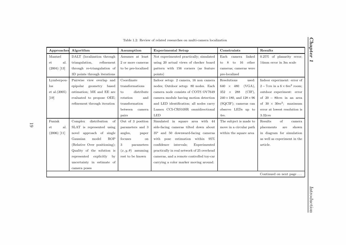
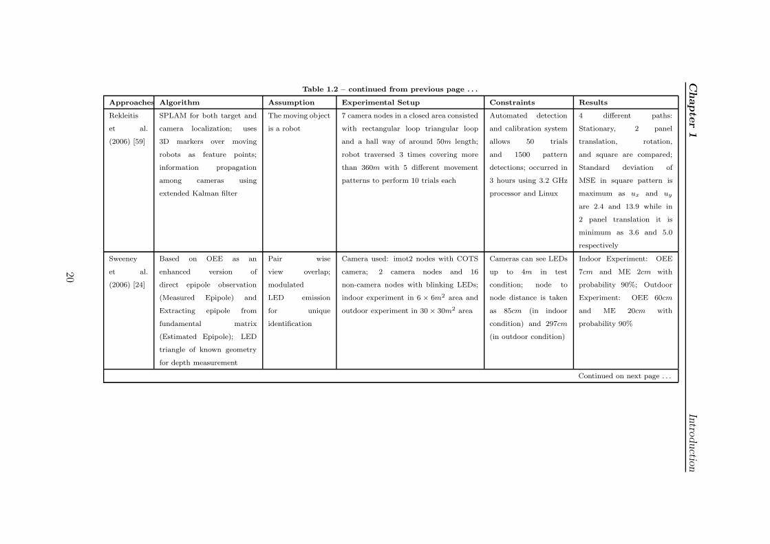
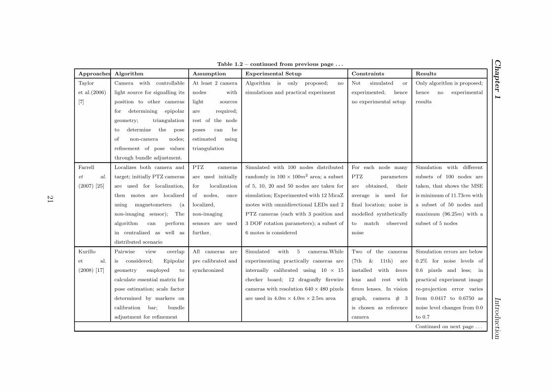
cost of feature point detection. Table 1.2 illustrates and compares few landmark
researches to portray the variety of algorithms used, assumptions, experimental
setups and results thus obtained. There has also been change in application
domain of camera-localization and hence the need of precise localization. 3D
localization addresses the issue of localizing more number of unknown parameters,
whereas previous 2D localization dealt with less number of unknown parameters
considering few parameters to be known. Sensing the availability of low-cost
cameras, parallel research is going to make the localization algorithms distributed
rather than centralized. Researches have also been perceived in the direction of
accurate localization in presence of noisy environments, e.g. less number of available
feature points, feature points on the visual boundaries of the cameras etc. These kind
of algorithms are useful when number of cameras in a network is very high. However,
scope for future research lies in achieving precision towards 3D pose calculation of
camera.
18
Chapter1
Intro
ductio
nTable 1.2: Review of related researches on multi-camera localization
Approaches Algorithm Assumption Experimental Setup Constraints Results
Mantzel
et al.
(2004) [13]
DALT (localization through
triangulation, refinement
through re-triangulation of
3D points through iterations
Assumes at least
2 or more cameras
to be pre-localized
Not experimented practically; simulated
using 20 actual views of checker board
pattern with 156 corners (as feature
points)
Each camera linked
to 8 to 16 other
cameras; cameras were
pre-localized
0.25% of planarity error;
14mm error in 3m scale
Lymberpou-
los
et al.(2005)
[19]
Pairwise view overlap and
epipolar geometry based
estimation; ME and EE are
evaluated to propose OEE;
refinement through iteration
Coordinate
transformations
to distribute
rotation and
transformation
between camera
pairs
Indoor setup: 2 camera, 16 non camera
nodes; Outdoor setup: 80 nodes. Each
camera node consists of COTS OV7649
camera module having motion detection
and LED identification; all nodes carry
Lumex CCI-CRS10SR omnidirectional
LED
Resolutions used:
640 × 480 (VGA),
352 × 288 (CIF),
240×180, and 128×96
(SQCIF); cameras can
observe LEDs up to
4m.
Indoor experiment: error of
2− 7cm in a 6× 6m2 room;
outdoor experiment: error
of 20 − 80cm in an area
of 30 × 30m2; maximum
error at lowest resolution is
3.32cm
Funiak
et al.
(2006) [11]
Complex distribution of
SLAT is represented using
novel approach of single
Gaussian model ROP
(Relative Over positioning);
Quality of the solution is
represented explicitly by
uncertainty in estimate of
camera poses
Out of 3 position
parameters and 3
angles, paper
focuses on
3 parameters
(x, y, θ) assuming
rest to be known
Simulated in square area with 44
side-facing cameras tilted down about
35° and 50 downward-facing cameras
with pose estimation within 95%
confidence intervals; Experimented
practically in real network of 25 overhead
cameras, and a remote controlled toy-car
carrying a color marker moving around.
The subject is made to
move in a circular path
within the square area
Results of camera
placements are shown
in diagram for simulation
as well as experiment in the
article.
Continued on next page . . .
19
Chapter1
Intro
ductio
nTable 1.2 – continued from previous page . . .
Approaches Algorithm Assumption Experimental Setup Constraints Results
Rekleitis
et al.
(2006) [59]
SPLAM for both target and
camera localization; uses
3D markers over moving
robots as feature points;
information propagation
among cameras using
extended Kalman filter
The moving object
is a robot
7 camera nodes in a closed area consisted
with rectangular loop triangular loop
and a hall way of around 50m length;
robot traversed 3 times covering more
than 360m with 5 different movement
patterns to perform 10 trials each
Automated detection
and calibration system
allows 50 trials
and 1500 pattern
detections; occurred in
3 hours using 3.2 GHz
processor and Linux
4 different paths:
Stationary, 2 panel
translation, rotation,
and square are compared;
Standard deviation of
MSE in square pattern is
maximum as ux and uy
are 2.4 and 13.9 while in
2 panel translation it is
minimum as 3.6 and 5.0
respectively
Sweeney
et al.
(2006) [24]
Based on OEE as an
enhanced version of
direct epipole observation
(Measured Epipole) and
Extracting epipole from
fundamental matrix
(Estimated Epipole); LED
triangle of known geometry
for depth measurement
Pair wise
view overlap;
modulated
LED emission
for unique
identification
Camera used: imot2 nodes with COTS
camera; 2 camera nodes and 16
non-camera nodes with blinking LEDs;
indoor experiment in 6 × 6m2 area and
outdoor experiment in 30× 30m2 area
Cameras can see LEDs
up to 4m in test
condition; node to
node distance is taken
as 85cm (in indoor
condition) and 297cm
(in outdoor condition)
Indoor Experiment: OEE
7cm and ME 2cm with
probability 90%; Outdoor
Experiment: OEE 60cm
and ME 20cm with
probability 90%
Continued on next page . . .
20
Chapter1
Intro
ductio
nTable 1.2 – continued from previous page . . .
Approaches Algorithm Assumption Experimental Setup Constraints Results
Taylor
et al.(2006)
[7]
Camera with controllable
light source for signalling its
position to other cameras
for determining epipolar
geometry; triangulation
to determine the pose
of non-camera nodes;
refinement of pose values
through bundle adjustment.
At least 2 camera
nodes with
light sources
are required;
rest of the node
poses can be
estimated using
triangulation
Algorithm is only proposed; no
simulations and practical experiment
Not simulated or
experimented; hence
no experimental setup
Only algorithm is proposed;
hence no experimental
results
Farrell
et al.
(2007) [25]
Localizes both camera and
target; initially PTZ cameras
are used for localization,
then motes are localized
using magnetometers (a
non-imaging sensor); The
algorithm can perform
in centralized as well as
distributed scenario
PTZ cameras
are used initially
for localization
of nodes, once
localized,
non-imaging
sensors are used
further.
Simulated with 100 nodes distributed
randomly in 100 × 100m2 area; a subset
of 5, 10, 20 and 50 nodes are taken for
simulation; Experimented with 12 MicaZ
motes with omnidirectional LEDs and 2
PTZ cameras (each with 3 position and
3 DOF rotation parameters); a subset of
6 motes is considered
For each node many
PTZ parameters
are obtained, their
average is used for
final location; noise is
modelled synthetically
to match observed
noise
Simulation with different
subsets of 100 nodes are
taken, that shows the MSE
is minimum of 11.73cm with
a subset of 50 nodes and
maximum (96.25m) with a
subset of 5 nodes
Kurillo
et al.
(2008) [17]
Pairwise view overlap
is considered; Epipolar
geometry employed to
calculate essential matrix for
pose estimation; scale factor
determined by markers on
calibration bar; bundle
adjustment for refinement
All cameras are
pre calibrated and
synchronized
Simulated with 5 cameras.While
experimenting practically cameras are
internally calibrated using 10 × 15
checker board; 12 dragonfly firewire
cameras with resolution 640× 480 pixels
are used in 4.0m× 4.0m × 2.5m area
Two of the cameras
(7th & 11th) are
installed with 4mm
lens and rest with
6mm lenses. In vision
graph, camera # 3
is chosen as reference
camera
Simulation errors are below
0.2% for noise levels of
0.6 pixels and less; in
practical experiment image
re-projection error varies
from 0.0417 to 0.6750 as
noise level changes from 0.0
to 0.7
Continued on next page . . .
21
Chapter1
Intro
ductio
nTable 1.2 – continued from previous page . . .
Approaches Algorithm Assumption Experimental Setup Constraints Results
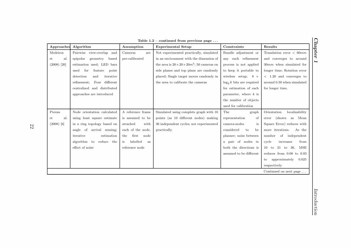
Medeiros
et al.
(2008) [20]
Pairwise view-overlap and
epipolar geometry based
estimation used; LED bars
used for feature point
detection and iterative
refinement; Four different
centralized and distributed
approaches are introduced
Cameras are
pre-calibrated
Not experimented practically, simulated
in an environment with the dimension of
the area is 20×20×20m3 ; 50 cameras on
side planes and top plane are randomly
placed; Single target moves randomly in
the area to calibrate the cameras
Bundle adjustment or
any such refinement
process is not applied
to keep it portable to
wireless setup; 8 ×
log2 k bits are required
for estimation of each
parameter, where k is
the number of objects
used for calibration
Translation error < 60mm
and converges to around
30mm when simulated for
longer time; Rotation error
< 1.20 and converges to
around 0.50 when simulated
for longer time.
Piovan
et al.
(2008) [6]
Node orientation calculated
using least square estimate
in a ring topology based on
angle of arrival sensing;
iterative estimation
algorithm to reduce the
effect of noise
A reference frame
is assumed to be
attached with
each of the node,
the first node
is labelled as
reference node
Simulated using complete graph with 10
points (as 10 different nodes) making
36 independent cycles; not experimented
practically.
The graph
representation of
camera-nodes is
considered to be
planner; noise between
a pair of nodes in
both the directions is
assumed to be different
Orientation localizability
error (shown as Mean
Square Error) reduces with
more iterations. As the
number of independent
cycle increases from
10 to 21 to 36, MSE
reduces from 0.08 to 0.03
to approximately 0.025
respectively
Continued on next page . . .
22
Chapter1
Intro
ductio
nTable 1.2 – continued from previous page . . .
Approaches Algorithm Assumption Experimental Setup Constraints Results
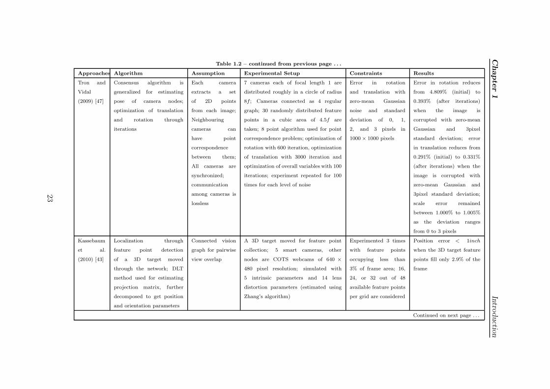
Tron and
Vidal
(2009) [47]
Consensus algorithm is
generalized for estimating
pose of camera nodes;
optimization of translation
and rotation through
iterations
Each camera
extracts a set
of 2D points
from each image;
Neighbouring
cameras can
have point
correspondence
between them;
All cameras are
synchronized;
communication
among cameras is
lossless
7 cameras each of focal length 1 are
distributed roughly in a circle of radius
8f ; Cameras connected as 4 regular
graph; 30 randomly distributed feature
points in a cubic area of 4.5f are
taken; 8 point algorithm used for point
correspondence problem; optimization of
rotation with 600 iteration, optimization
of translation with 3000 iteration and
optimization of overall variables with 100
iterations; experiment repeated for 100
times for each level of noise
Error in rotation
and translation with
zero-mean Gaussian
noise and standard
deviation of 0, 1,
2, and 3 pixels in
1000 × 1000 pixels
Error in rotation reduces
from 4.809% (initial) to
0.393% (after iterations)
when the image is
corrupted with zero-mean
Gaussian and 3pixel
standard deviation; error
in translation reduces from
0.291% (initial) to 0.331%
(after iterations) when the
image is corrupted with
zero-mean Gaussian and
3pixel standard deviation;
scale error remained
between 1.000% to 1.005%
as the deviation ranges
from 0 to 3 pixels
Kassebaum
et al.
(2010) [43]
Localization through
feature point detection
of a 3D target moved
through the network; DLT
method used for estimating
projection matrix, further
decomposed to get position
and orientation parameters
Connected vision
graph for pairwise
view overlap
A 3D target moved for feature point
collection; 5 smart cameras, other
nodes are COTS webcams of 640 ×
480 pixel resolution; simulated with
5 intrinsic parameters and 14 lens
distortion parameters (estimated using
Zhang’s algorithm)
Experimented 3 times
with feature points
occupying less than
3% of frame area; 16,
24, or 32 out of 48
available feature points
per grid are considered
Position error < 1inch
when the 3D target feature
points fill only 2.9% of the
frame
Continued on next page . . .
23
Chapter1
Intro
ductio
nTable 1.2 – continued from previous page . . .
Approaches Algorithm Assumption Experimental Setup Constraints Results
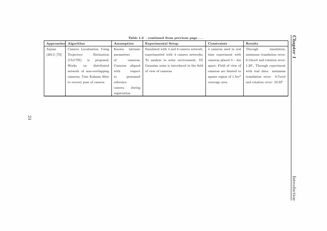
Anjum
(2011) [73]
Camera Localization Using
Trajectory Estimation
(CLUTE) is proposed;
Works on distributed
network of non-overlapping
cameras; Uses Kalman filter
to recover pose of camera
Known intrinsic
parameters
of cameras;
Cameras aligned
with respect
to presumed
reference
camera during
registration
Simulated with 4 and 8 camera network,
experimented with 4 camera networks;
To analyse in noisy environment, 5%
Gaussian noise is introduced in the field
of view of cameras
4 cameras used in real
time experiment with
cameras placed 3− 4m
apart; Field of view of
cameras are limited to
square region of 1.5m2
coverage area
Through simulation,
minimum translation error:
0.13unit and rotation error:
1.29°; Through experiment
with real data: minimum
translation error: 0.7unit
and rotation error: 10.33°
24
Chapter 1 Introduction
1.2.2 Camera Placement for Gait Based Identification
Since the evolution of MCN; and with the increasing affordability and adaptability
of the system, many novel applications of MCN are developed. Sensing rooms,
assisted living for old age or disabled people, immersive conference rooms, coverage
and telecast of games and diverse applications in visual surveillance are to name
a few. With difference in priority of coverage, types and numbers of camera
and geographical conditions of coverage area, the placement of camera becomes
an important issue of research. Moreover, as the number of camera in such
system grows, the development of automatic camera placement technique becomes
very essential. Optimizing the placement of camera not only reduces the cost of
installation, but also increases the suitability of the system for specific task, thus
increasing its performance efficiency.
Approach towards achieving suitability in the camera placement depends on the
task MCN is intended for. Some of the strategies for camera placement with different
goals are:
(i) Minimizing the number of camera, to cover a given area.This type of constraint
helps in lowering the installation cost by reducing the number of camera.
(ii) Maximizing the coverage area with fixed number of camera. This type of
constraint helps in increasing coverage with fixed number of cameras thus
providing best coverage with given number and type of camera
(iii) Covering a human subject with maximum frontal view. This kind of
constraints gives better result in face identification, gesture recognition, and
visual tagging.
(iv) Covering for maximum orthogonal view. This kind of constraints are useful in
surveillance oriented task like identification through gait patterns, occlusion
handling while object tracking, height, and profile face based identification.
25
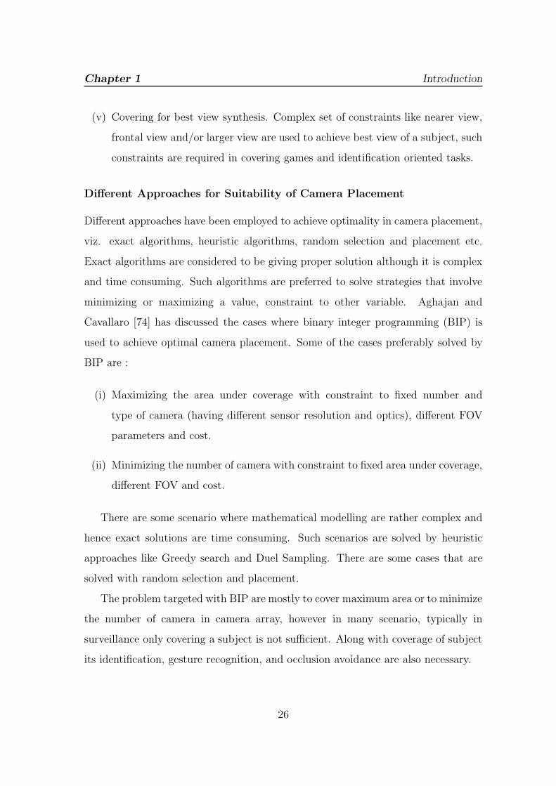
Chapter 1 Introduction
(v) Covering for best view synthesis. Complex set of constraints like nearer view,
frontal view and/or larger view are used to achieve best view of a subject, such
constraints are required in covering games and identification oriented tasks.
Different Approaches for Suitability of Camera Placement
Different approaches have been employed to achieve optimality in camera placement,
viz. exact algorithms, heuristic algorithms, random selection and placement etc.
Exact algorithms are considered to be giving proper solution although it is complex
and time consuming. Such algorithms are preferred to solve strategies that involve
minimizing or maximizing a value, constraint to other variable. Aghajan and
Cavallaro [74] has discussed the cases where binary integer programming (BIP) is
used to achieve optimal camera placement. Some of the cases preferably solved by
BIP are :
(i) Maximizing the area under coverage with constraint to fixed number and
type of camera (having different sensor resolution and optics), different FOV
parameters and cost.
(ii) Minimizing the number of camera with constraint to fixed area under coverage,
different FOV and cost.
There are some scenario where mathematical modelling are rather complex and
hence exact solutions are time consuming. Such scenarios are solved by heuristic
approaches like Greedy search and Duel Sampling. There are some cases that are
solved with random selection and placement.
The problem targeted with BIP are mostly to cover maximum area or to minimize
the number of camera in camera array, however in many scenario, typically in
surveillance only covering a subject is not sufficient. Along with coverage of subject
its identification, gesture recognition, and occlusion avoidance are also necessary.
26
Chapter 1 Introduction
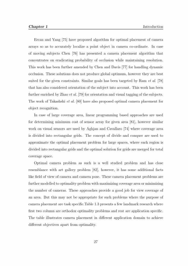
Ercan and Yang [75] have proposed algorithm for optimal placement of camera
arrays so as to accurately localize a point object in camera co-ordinate. In case
of moving subjects Chen [76] has presented a camera placement algorithm that
concentrates on eradicating probability of occlusion while maintaining resolution.
This work has been further amended by Chen and Davis [77] for handling dynamic
occlusion. These solutions does not produce global optimum, however they are best
suited for the given constraints. Similar goals has been targeted by Ram et al. [78]
that has also considered orientation of the subject into account. This work has been
further enriched by Zhao et al. [79] for orientation and visual tagging of the subjects.
The work of Takashshi et al. [80] have also proposed optimal camera placement for
object recognition.
In case of large coverage area, linear programming based approaches are used
for determining minimum cost of sensor array for given area [81], however similar
work on visual sensors are used by Aghjan and Cavallaro [74] where coverage area
is divided into rectangular grids. The concept of divide and conquer are used to
approximate the optimal placement problem for large spaces, where each region is
divided into rectangular grids and the optimal solution for grids are merged for total
coverage space.
Optimal camera problem as such is a well studied problem and has close
resemblance with art gallery problem [82], however, it has some additional facts
like field of view of camera and camera pose. These camera placement problems are
further modelled to optimality problem with maximizing coverage area or minimizing
the number of cameras. These approaches provide a good job for view coverage of
an area. But this may not be appropriate for such problems where the purpose of
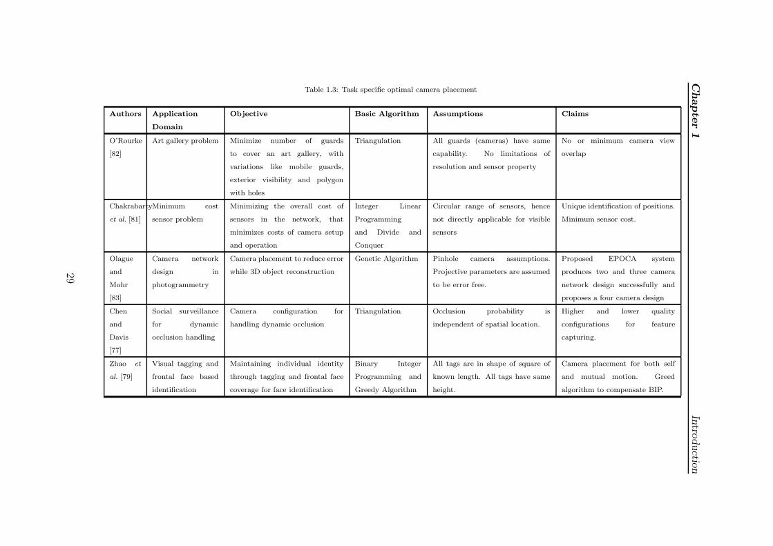
camera placement are task specific.Table 1.3 presents a few landmark research where
first two column are orthodox optimality problems and rest are application specific.
The table illustrates camera placement in different application domain to achieve
different objectives apart from optimality.
27
Chapter 1 Introduction
The proposed multi-camera based surveillance model presented in this thesis has
the goal of subject identification and uninterrupted track of the subject. In chapter 3,
a divide and conquer based method for efficient camera placement has been presented
that finds suitable camera placement for gait pattern and height based identification.
It has been justified with a conducted experiment that orthogonal view of a camera
is best suited for height and gait pattern based identification. The large coverage
area is divided into rectangular grids and solution for each grid is merged to get final
camera placement.
28
Chapter1
Intro
ductio
nTable 1.3: Task specific optimal camera placement
Authors Application
Domain
Objective Basic Algorithm Assumptions Claims
O’Rourke
[82]
Art gallery problem Minimize number of guards
to cover an art gallery, with
variations like mobile guards,
exterior visibility and polygon
with holes
Triangulation All guards (cameras) have same
capability. No limitations of
resolution and sensor property
No or minimum camera view
overlap
Chakrabarty
et al. [81]
Minimum cost
sensor problem
Minimizing the overall cost of
sensors in the network, that
minimizes costs of camera setup
and operation
Integer Linear
Programming
and Divide and
Conquer
Circular range of sensors, hence
not directly applicable for visible
sensors
Unique identification of positions.
Minimum sensor cost.
Olague
and
Mohr
[83]
Camera network
design in
photogrammetry
Camera placement to reduce error
while 3D object reconstruction
Genetic Algorithm Pinhole camera assumptions.
Projective parameters are assumed
to be error free.
Proposed EPOCA system
produces two and three camera
network design successfully and
proposes a four camera design
Chen
and
Davis
[77]
Social surveillance
for dynamic
occlusion handling
Camera configuration for
handling dynamic occlusion
Triangulation Occlusion probability is
independent of spatial location.
Higher and lower quality
configurations for feature
capturing.
Zhao et
al. [79]
Visual tagging and
frontal face based
identification
Maintaining individual identity
through tagging and frontal face
coverage for face identification
Binary Integer
Programming and
Greedy Algorithm
All tags are in shape of square of
known length. All tags have same
height.
Camera placement for both self
and mutual motion. Greed
algorithm to compensate BIP.
29
Chapter 1 Introduction
1.2.3 Camera Control for Occlusion Avoidance
For an MCN system that aims towards optimal usage of its resources, the efficient
handling and control of the system is as important as the localization and task
specific placement of camera. The previous sections of this chapter so far discuss
the developments in the mode of camera calibration in the form of an extensive
survey and discusses different approaches for finding suitable placement of cameras
in diverse contexts. This section presents a study on different approaches towards
handling occlusion in different camera models.
The efforts in technological growth have made way for the emergence of variety
of methodologies for tracking objects in diverse contexts. Different algorithms have
been designed for different requirements depending upon the mode of tracking,
location, significance and specific needs. The earlier tracking approaches have
implemented several image processing algorithms on the video output from a single
camera. Contour based tracking, background subtraction based tracking, Gaussian
based tracking, median filter based tracking, are some of the most studied and refined
technologies among them [84]. These algorithms are simple in implementation, fast
in processing and analysis. However, they are limited with constant field of view
and suffer from occlusion of the tracked subject.
As the demand for fool-proof tracking algorithm prevailed so is the paradigm
shifted from single to multi-camera model. These systems are more useful for
tracking in crowded places and highly protected areas. This can be equipped with
a variety of cameras and distributed processors to even amend the functionality
of tracking. But multi-camera systems have their complexities and trade-offs.
As compared with single camera tracking, multi-camera tracking needs additional
processing, extra memory requirement, superfluous energy consumption, higher
installation cost, and complex handling and implementation.
Occlusion handling is one of the major problems in single camera based tracking.
In the model proposed by Sinior et al. [85] background subtraction is used for object
30
Chapter 1 Introduction
tracking and occlusion detection. It uses appearance based model to estimate the
centroid of the moving object more accurately. This technique is although reliable
but works with fixed background. Authors in [86, 87] have handled occlusion based
on measurement error for each pixel. Authors in [88] have devised a motion based
tracking algorithm that is adaptive with natural changes in appearance or variation
in 3D pose and hence remain robust with occlusion but does not resolve or predict
occlusion. In [89] two different approaches to cope occlusion are proposed; one
using evaluation of correlation error in templates and other using infra-red images
to detect occluded region by human hand. Authors in [90] have exploited contextual
information; it does better occlusion analysis but has tracking errors. It uses block
motion vectors for calculating object boundary to predict occlusion. Amizquita et
al. [91] have proposed an algorithm for auto detection of occlusion using motion
based prediction of objects movement during the stages of entering occlusion, full
occlusion, and exit occlusion.
On the other hand a multi-camera system can avoid occlusion and can provide
robust tracking but are not as simple and energy-efficient as single camera systems.
Although a camera system installed in master-slave mode [74], can achieve some level
of efficiency but the entire region under coverage should come under master cameras
view. Towards making the multi-camera model as an efficient approach a few other
works have also been proposed. Kulkarni et al. [1] have proposed an approach
for efficient use of multiple cameras by devising multi-tier camera network called
SensEye [2]. This approach is energy efficient although it has a complex hardware
architecture and diverse software requirement. It is observed from the literature that
single camera based object tracking is simple, energy efficient and has the ability to
predict occlusion. However, there is no scope for occlusion avoidance. To alleviate
the occlusion occurrence, a multi-camera model is necessary where the field of view
is tracked by multiple cameras. Generally, a multi-camera based approach utilizes
the cameras always in the active mode. But this leads to energy inefficiency and
31
Chapter 1 Introduction
more processing requirement. Our approach, as discussed in chapter 3 has been
been designed to bridge the gap between single camera and multi-camera based
surveillance system.
1.3 Thesis Organization
The rest of the thesis is organised as:
Chapter 2: Study on Efficient Camera Placement Techniques Placement
of camera is a vital step while bringing efficiency in camera usage of MCN.
The camera placement techniques changes vastly depending on the deployment
conditions like limited number of cameras, constraint of area under cover, condition
of best view synthesis, 3D image reconstruction or condition of gait based
identification. This chapter studies the importance of camera placement in bringing
optimality in camera usage of MCN. An efficient camera placement algorithm has
been proposed taking gait based identification as test condition. Simulation has
been performed and results have been presented towards the proposed algorithm.
Chapter 3: Study on Smart Camera Control Camera control is a crucial
stage in MCN. It defines conditions that governs the control among the cameras
in an MCN. A resource efficient MCN based surveillance model has been presented
that is governed by proposed occlusion determination algorithm. The proposed
algorithm determines the chances of occlusion, position and time to occlusion in
prior so that necessary action can be taken towards its mitigation. The proposal has
been experimentally justified on self acquired as well as publicly available database.
Chapter 4: Conclusion This chapter provides the concluding remarks with a
stress on achievements and limitations of the proposed schemes. The scopes for
further research are outlined at the end.
32
Chapter 2
Study on Efficient Camera
Placement Techniques
Placement of camera is a vital issue towards development of multi-camera based
smart surveillance system. Previous chapter highlights the necessity of calibration
for efficient operation and smart handling of MCN. Camera placement along with
its calibration completes the infrastructure of Multi-Camera Network (MCN). An
MCN designed with the goal of surveillance must provide uninterrupted track and
prospect for subject’s identification. This chapter proposes a camera placement
technique with a task of capturing orthogonal view of the subject that creates the
prospect of identification based on gait, height and profile face of a subject for the
sake of surveillance. Placement of camera is very crucial in surveillance. A suitably
placed array of camera brings two way benefits for the system, cost optimization of
MCN and enhanced performance due to tailor made camera placement approach for
specific task.
In the proposed surveillance model presented in this thesis, efficiency at the
level of camera placement has been identified as an important measure for achieving
33

Chapter 2 Study on Efficient Camera Placement Techniques
the goal of optimal multi-camera set-up without compromising with standards of
surveillance. The proposed model is considered to be performing identification of
moving subject through its gait patterns, its height and profile face, and also ensuring
uninterrupted track of the subject. With these goals, cameras are proposed to be
placed in such a way that it finds the path of the moving subject orthogonal to
the view axis of the camera. Further sections discuss about the unique behavioural
biometric feature called gait; which is a special cyclic pattern an individual repeats
during a walk. It has been justified through conducting an experiment and also
through the support of some existing results that orthogonal view is suggested as best
view for capturing gait information. Further, a novel approach has been presented
for estimating the best place for camera placement in an open space, with maximum
chances of capturing subjects’ movement orthogonal to the walk direction. This
proposal is been experimentally conducted at Vikram Sarabhai Hall of Residence,
NIT Rourkela and the model has been justified with proper results.
Section 2.1 presents introduction to gait biometric. Section 2.2 proposes a novel
approach of camera placement for gait pattern based identification. The experiment
towards the proposed model has been presented in Section 2.3. A few conclusive
remarks based on the experiment are discussed towards the end in Section 2.4.
2.1 Gait Biometric
Locomotion of an individual which is repetitive with same frequency and carries a
temporal pattern is termed as gait [92]. Walk, trot, run, and to climb stairs are
among such locomotion in which an individual has a temporal pattern that repeats
with same frequency. This makes these activities candidates for being gait.
The earlier progress towards establishing gait as a biometric trait is successor
to the research of Johansson [93] where experiments have been performed to
differentiate among different human postures by examining 10-12 nodal points over
34
Chapter 2 Study on Efficient Camera Placement Techniques
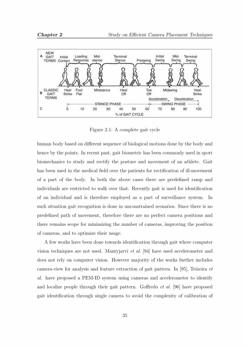
Figure 2.1: A complete gait cycle
human body based on different sequence of biological motions done by the body and
hence by the points. In recent past, gait biometric has been commonly used in sport
biomechanics to study and rectify the posture and movement of an athlete. Gait
has been used in the medical field over the patients for rectification of ill-movement
of a part of the body. In both the above cases there are predefined ramp and
individuals are restricted to walk over that. Recently gait is used for identification
of an individual and is therefore employed as a part of surveillance system. In
such situation gait recognition is done in unconstrained scenarios. Since there is no
predefined path of movement, therefore there are no perfect camera positions and
there remains scope for minimizing the number of cameras, improving the position
of cameras, and to optimize their usage.
A few works have been done towards identification through gait where computer
vision techniques are not used. Mantyjarvi et al. [94] have used accelerometer and
does not rely on computer vision. However majority of the works further includes
camera-view for analysis and feature extraction of gait pattern. In [95], Teixeira et
al. have proposed a PEM-ID system using cameras and accelerometer to identify
and localize people through their gait pattern. Goffredo et al. [96] have proposed
gait identification through single camera to avoid the complexity of calibration of
35
Chapter 2 Study on Efficient Camera Placement Techniques
multiple cameras. Bouchrika et al. [97] have presented a new approach for tracking
and identification between different non-intersecting uncalibrated cameras based on
gait pattern analysis. Jeges et al. [98] have worked towards estimating human height
in calibrated cameras that can be used as a supportive feature for identification. This
justifies why camera placement plays a crucial role for gait analysis in unconstraint
scenario.
A camera can best capture the gait features when it is placed orthogonal with
respect to the motion of the subject. Such positions of camera also make tracking
easier and are best placed for height measurement. Our proposed model has an
overhead-camera that prepares a path-band, based on the locus of various subjects
traversed over a span of time. Other field-cameras are PTZ cameras that are
placed at such positions where they can get maximum orthogonal views. These
positions are estimated by overhead-camera using the proposed algorithm and
path-band information. Further camera set-up works in master-slave mode so that
overhead-camera guides field-cameras to track the target efficiently. Section 2 of
this chapter states the problem under consideration in detail. The subsequent steps
of proposed model towards the solution of the problem are illustrated in Section 3.
Section 4 presents the experiment conducted towards the proposed model. The result
of the experiment has been presented in Section 5. Finally, Section 6 concludes the
chapter along with stating the scope for future works towards the proposed model.
2.2 Proposed Model
When a camera network is set-up to identify a subject walking in a given area, the
locus of the subject is not known in prior. Hence best positions for camera placement
cannot be statically defined. If a most probable path can be estimated based on paths
traversed earlier, then camera placement can be done efficiently. Secondly, there can
be an effort to find the minimal number of cameras along with their poses to cover
36
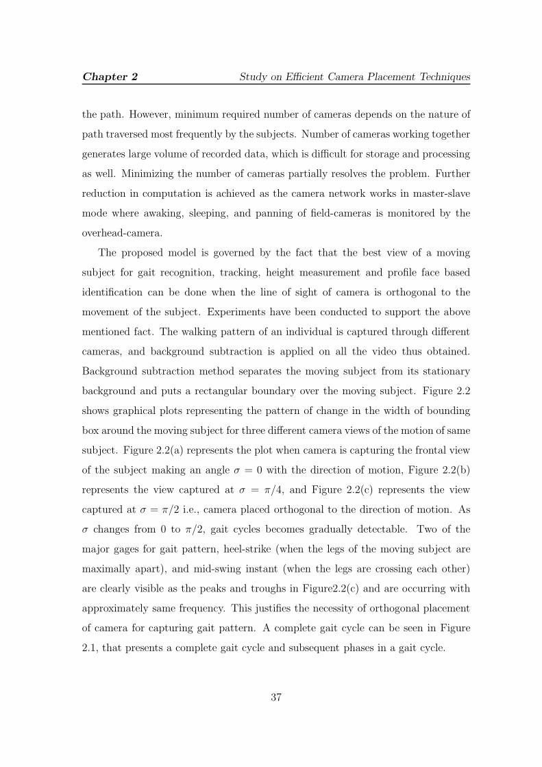
Chapter 2 Study on Efficient Camera Placement Techniques
the path. However, minimum required number of cameras depends on the nature of
path traversed most frequently by the subjects. Number of cameras working together
generates large volume of recorded data, which is difficult for storage and processing
as well. Minimizing the number of cameras partially resolves the problem. Further
reduction in computation is achieved as the camera network works in master-slave
mode where awaking, sleeping, and panning of field-cameras is monitored by the
overhead-camera.
The proposed model is governed by the fact that the best view of a moving
subject for gait recognition, tracking, height measurement and profile face based
identification can be done when the line of sight of camera is orthogonal to the
movement of the subject. Experiments have been conducted to support the above
mentioned fact. The walking pattern of an individual is captured through different
cameras, and background subtraction is applied on all the video thus obtained.
Background subtraction method separates the moving subject from its stationary
background and puts a rectangular boundary over the moving subject. Figure 2.2
shows graphical plots representing the pattern of change in the width of bounding
box around the moving subject for three different camera views of the motion of same
subject. Figure 2.2(a) represents the plot when camera is capturing the frontal view
of the subject making an angle σ = 0 with the direction of motion, Figure 2.2(b)
represents the view captured at σ = π/4, and Figure 2.2(c) represents the view
captured at σ = π/2 i.e., camera placed orthogonal to the direction of motion. As
σ changes from 0 to π/2, gait cycles becomes gradually detectable. Two of the
major gages for gait pattern, heel-strike (when the legs of the moving subject are
maximally apart), and mid-swing instant (when the legs are crossing each other)
are clearly visible as the peaks and troughs in Figure2.2(c) and are occurring with
approximately same frequency. This justifies the necessity of orthogonal placement
of camera for capturing gait pattern. A complete gait cycle can be seen in Figure
2.1, that presents a complete gait cycle and subsequent phases in a gait cycle.
37
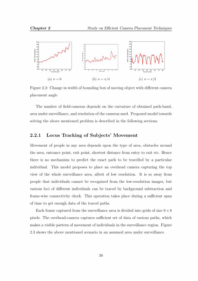
Chapter 2 Study on Efficient Camera Placement Techniques
10 20 30 40 50 60 70 8050
60
70
80
90
100
110
120
130
140
150
160
Frame Number
Wid
th o
f B
ou
nd
ing
Bo
x
(a) σ = 0
10 20 30 40 50 60 70 8050
60
70
80
90
100
110
120
130
140
150
160
Frame Number
Wid
th o
f Bou
ndin
g B
ox
(b) σ = π/4
10 20 30 40 50 60 70 8050
60
70
80
90
100
110
120
130
140
150
160
Frame Number
Wid
th o
f Bou
ndin
g B
ox
(c) σ = π/2
Figure 2.2: Change in width of bounding box of moving object with different camera
placement angle
The number of field-cameras depends on the curvature of obtained path-band,
area under surveillance, and resolution of the cameras used. Proposed model towards
solving the above mentioned problem is described in the following sections.
2.2.1 Locus Tracking of Subjects’ Movement
Movement of people in any area depends upon the type of area, obstacles around
the area, entrance point, exit point, shortest distance from entry to exit etc. Hence
there is no mechanism to predict the exact path to be travelled by a particular
individual. This model proposes to place an overhead camera capturing the top
view of the whole surveillance area, albeit of low resolution. It is so away from
people that individuals cannot be recognized from the low-resolution images, but
various loci of different individuals can be traced by background subtraction and
frame-wise connectivity check. This operation takes place during a sufficient span
of time to get enough data of the traced paths.
Each frame captured from the surveillance area is divided into grids of size 8× 8
pixels. The overhead-camera captures sufficient set of data of various paths, which
makes a visible pattern of movement of individuals in the surveillance region. Figure
2.3 shows the above mentioned scenario in an assumed area under surveillance.
38
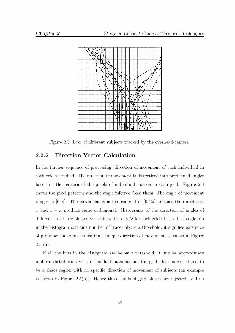
Chapter 2 Study on Efficient Camera Placement Techniques
Figure 2.3: Loci of different subjects tracked by the overhead-camera
2.2.2 Direction Vector Calculation
In the further sequence of processing, direction of movement of each individual in
each grid is studied. The direction of movement is discretized into predefined angles
based on the pattern of the pixels of individual motion in each grid. Figure 2.4
shows the pixel patterns and the angle inferred from them. The angle of movement
ranges in [0, π]. The movement is not considered in [0, 2π] because the directions:
x and x + π produce same orthogonal. Histograms of the direction of angles of
different traces are plotted with bin-width of π/8 for each grid blocks. If a single bin
in the histogram contains number of traces above a threshold, it signifies existence
of prominent maxima indicating a unique direction of movement as shown in Figure
2.5 (a).
If all the bins in the histogram are below a threshold, it implies approximate
uniform distribution with no explicit maxima and the grid block is considered to
be a chaos region with no specific direction of movement of subjects (an example
is shown in Figure 2.5(b)). Hence these kinds of grid blocks are rejected, and no
39
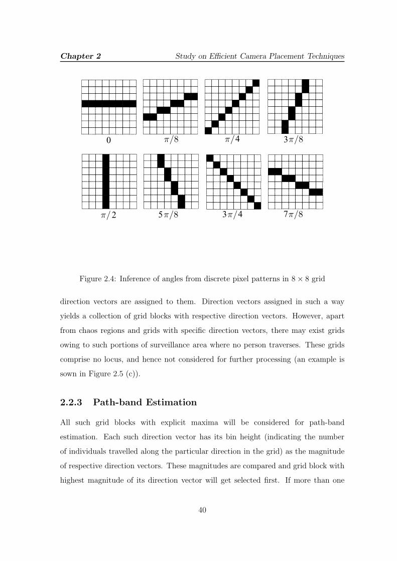
Chapter 2 Study on Efficient Camera Placement Techniques
0
35
4 3
2 4 7
Figure 2.4: Inference of angles from discrete pixel patterns in 8× 8 grid
direction vectors are assigned to them. Direction vectors assigned in such a way
yields a collection of grid blocks with respective direction vectors. However, apart
from chaos regions and grids with specific direction vectors, there may exist grids
owing to such portions of surveillance area where no person traverses. These grids
comprise no locus, and hence not considered for further processing (an example is
sown in Figure 2.5 (c)).
2.2.3 Path-band Estimation
All such grid blocks with explicit maxima will be considered for path-band
estimation. Each such direction vector has its bin height (indicating the number
of individuals travelled along the particular direction in the grid) as the magnitude
of respective direction vectors. These magnitudes are compared and grid block with
highest magnitude of its direction vector will get selected first. If more than one
40
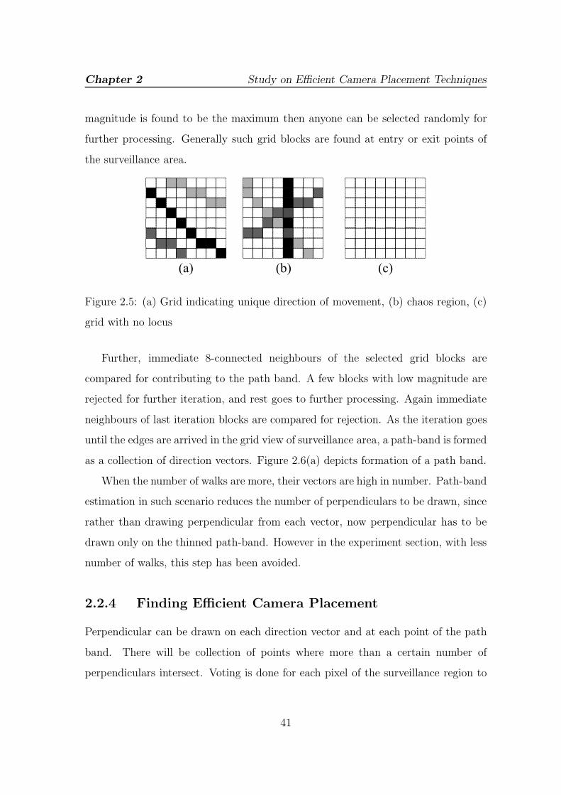
Chapter 2 Study on Efficient Camera Placement Techniques
magnitude is found to be the maximum then anyone can be selected randomly for
further processing. Generally such grid blocks are found at entry or exit points of
the surveillance area.
(a) (b) (c)
Figure 2.5: (a) Grid indicating unique direction of movement, (b) chaos region, (c)
grid with no locus
Further, immediate 8-connected neighbours of the selected grid blocks are
compared for contributing to the path band. A few blocks with low magnitude are
rejected for further iteration, and rest goes to further processing. Again immediate
neighbours of last iteration blocks are compared for rejection. As the iteration goes
until the edges are arrived in the grid view of surveillance area, a path-band is formed
as a collection of direction vectors. Figure 2.6(a) depicts formation of a path band.
When the number of walks are more, their vectors are high in number. Path-band
estimation in such scenario reduces the number of perpendiculars to be drawn, since
rather than drawing perpendicular from each vector, now perpendicular has to be
drawn only on the thinned path-band. However in the experiment section, with less
number of walks, this step has been avoided.
2.2.4 Finding Efficient Camera Placement
Perpendicular can be drawn on each direction vector and at each point of the path
band. There will be collection of points where more than a certain number of
perpendiculars intersect. Voting is done for each pixel of the surveillance region to
41
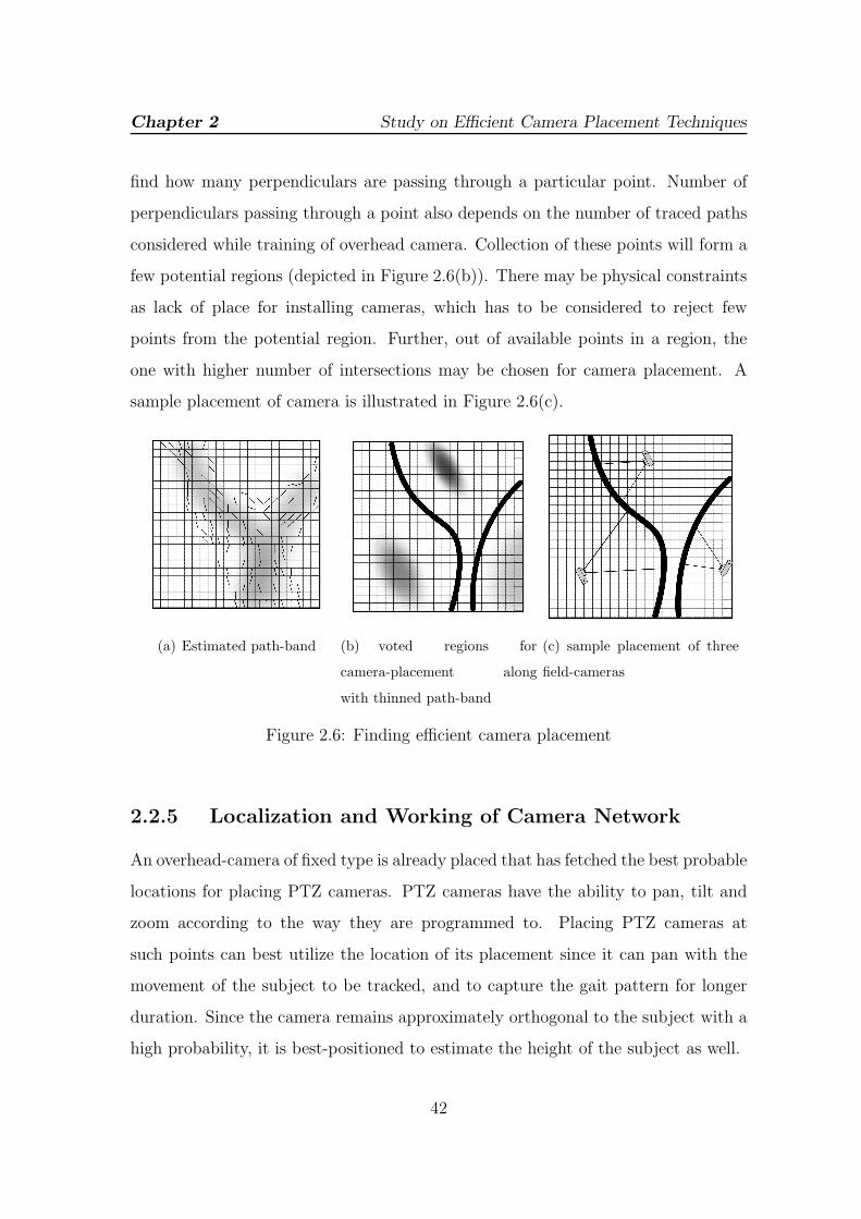
Chapter 2 Study on Efficient Camera Placement Techniques
find how many perpendiculars are passing through a particular point. Number of
perpendiculars passing through a point also depends on the number of traced paths
considered while training of overhead camera. Collection of these points will form a
few potential regions (depicted in Figure 2.6(b)). There may be physical constraints
as lack of place for installing cameras, which has to be considered to reject few
points from the potential region. Further, out of available points in a region, the
one with higher number of intersections may be chosen for camera placement. A
sample placement of camera is illustrated in Figure 2.6(c).
(a) Estimated path-band (b) voted regions for
camera-placement along
with thinned path-band
(c) sample placement of three
field-cameras
Figure 2.6: Finding efficient camera placement
2.2.5 Localization and Working of Camera Network
An overhead-camera of fixed type is already placed that has fetched the best probable
locations for placing PTZ cameras. PTZ cameras have the ability to pan, tilt and
zoom according to the way they are programmed to. Placing PTZ cameras at
such points can best utilize the location of its placement since it can pan with the
movement of the subject to be tracked, and to capture the gait pattern for longer
duration. Since the camera remains approximately orthogonal to the subject with a
high probability, it is best-positioned to estimate the height of the subject as well.
42
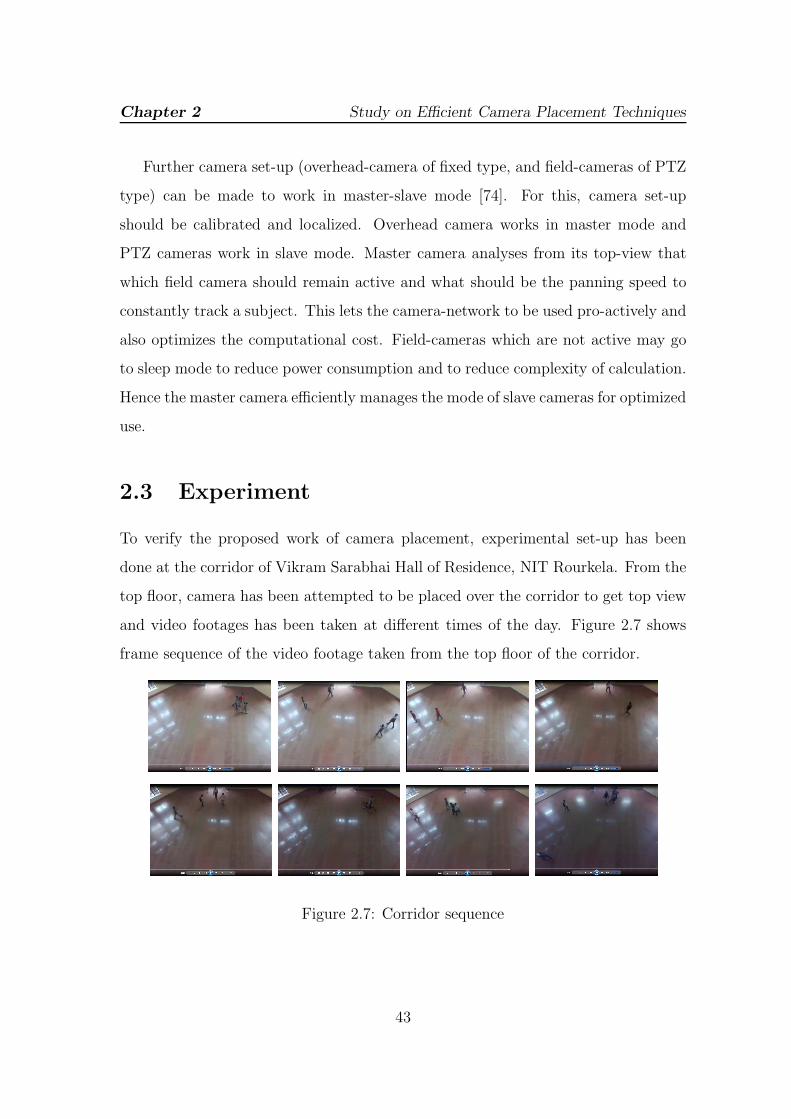
Chapter 2 Study on Efficient Camera Placement Techniques
Further camera set-up (overhead-camera of fixed type, and field-cameras of PTZ
type) can be made to work in master-slave mode [74]. For this, camera set-up
should be calibrated and localized. Overhead camera works in master mode and
PTZ cameras work in slave mode. Master camera analyses from its top-view that
which field camera should remain active and what should be the panning speed to
constantly track a subject. This lets the camera-network to be used pro-actively and
also optimizes the computational cost. Field-cameras which are not active may go
to sleep mode to reduce power consumption and to reduce complexity of calculation.
Hence the master camera efficiently manages the mode of slave cameras for optimized
use.
2.3 Experiment
To verify the proposed work of camera placement, experimental set-up has been
done at the corridor of Vikram Sarabhai Hall of Residence, NIT Rourkela. From the
top floor, camera has been attempted to be placed over the corridor to get top view
and video footages has been taken at different times of the day. Figure 2.7 shows
frame sequence of the video footage taken from the top floor of the corridor.
Figure 2.7: Corridor sequence
43
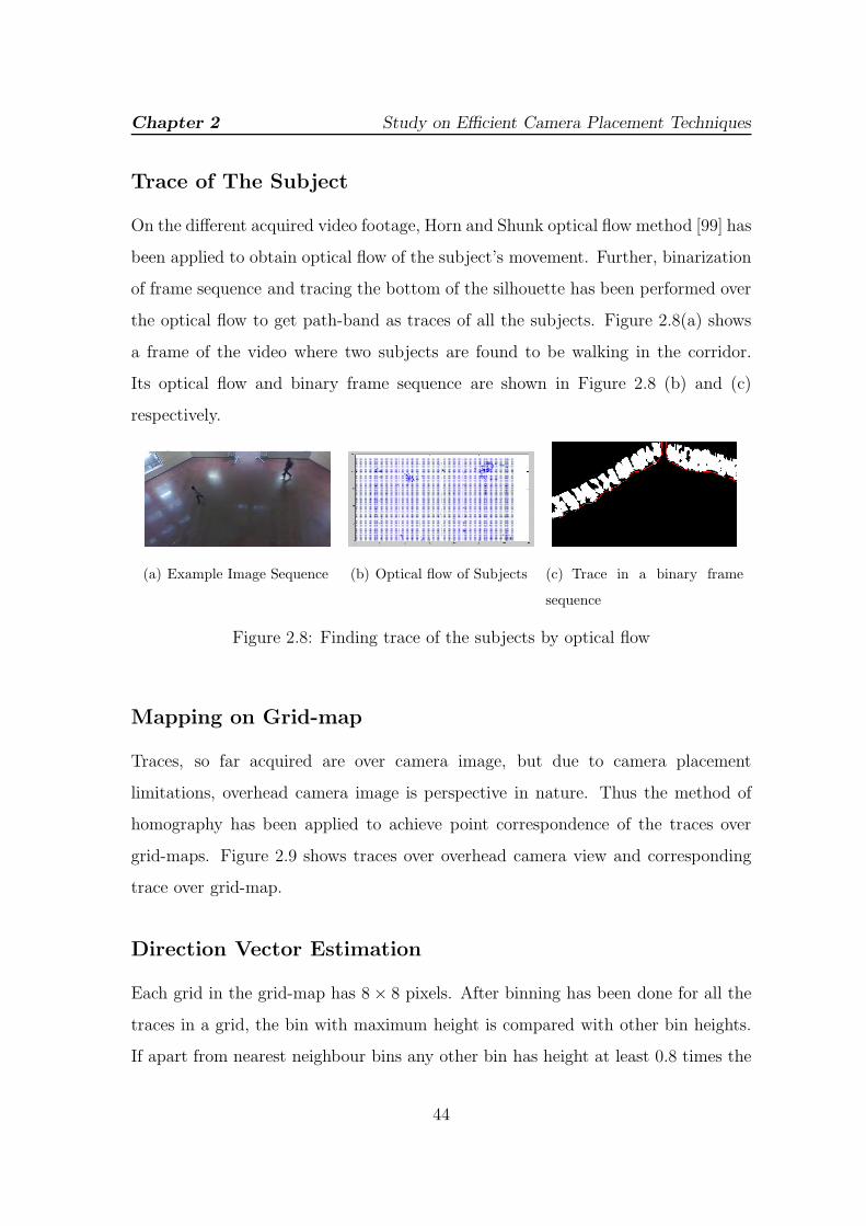
Chapter 2 Study on Efficient Camera Placement Techniques
Trace of The Subject
On the different acquired video footage, Horn and Shunk optical flow method [99] has
been applied to obtain optical flow of the subject’s movement. Further, binarization
of frame sequence and tracing the bottom of the silhouette has been performed over
the optical flow to get path-band as traces of all the subjects. Figure 2.8(a) shows
a frame of the video where two subjects are found to be walking in the corridor.
Its optical flow and binary frame sequence are shown in Figure 2.8 (b) and (c)
respectively.
(a) Example Image Sequence (b) Optical flow of Subjects (c) Trace in a binary frame
sequence
Figure 2.8: Finding trace of the subjects by optical flow
Mapping on Grid-map
Traces, so far acquired are over camera image, but due to camera placement
limitations, overhead camera image is perspective in nature. Thus the method of
homography has been applied to achieve point correspondence of the traces over
grid-maps. Figure 2.9 shows traces over overhead camera view and corresponding
trace over grid-map.
Direction Vector Estimation
Each grid in the grid-map has 8× 8 pixels. After binning has been done for all the
traces in a grid, the bin with maximum height is compared with other bin heights.
If apart from nearest neighbour bins any other bin has height at least 0.8 times the
44
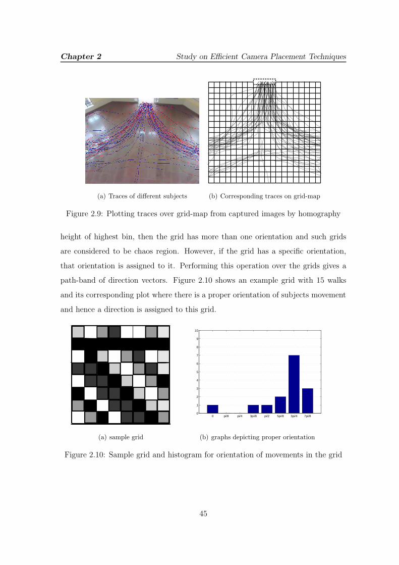
Chapter 2 Study on Efficient Camera Placement Techniques
(a) Traces of different subjects (b) Corresponding traces on grid-map
Figure 2.9: Plotting traces over grid-map from captured images by homography
height of highest bin, then the grid has more than one orientation and such grids
are considered to be chaos region. However, if the grid has a specific orientation,
that orientation is assigned to it. Performing this operation over the grids gives a
path-band of direction vectors. Figure 2.10 shows an example grid with 15 walks
and its corresponding plot where there is a proper orientation of subjects movement
and hence a direction is assigned to this grid.
(a) sample grid
0 pi/8 pi/4 3pi/8 pi/2 5pi/8 3pi/4 7pi/80
1
2
3
4
5
6
7
8
9
10
(b) graphs depicting proper orientation
Figure 2.10: Sample grid and histogram for orientation of movements in the grid
45
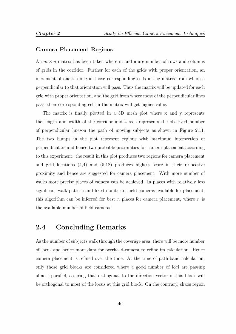
Chapter 2 Study on Efficient Camera Placement Techniques
Camera Placement Regions
An m × n matrix has been taken where m and n are number of rows and columns
of grids in the corridor. Further for each of the grids with proper orientation, an
increment of one is done in those corresponding cells in the matrix from where a
perpendicular to that orientation will pass. Thus the matrix will be updated for each
grid with proper orientation, and the grid from where most of the perpendicular lines
pass, their corresponding cell in the matrix will get higher value.
The matrix is finally plotted in a 3D mesh plot where x and y represents
the length and width of the corridor and z axis represents the observed number
of perpendicular lineson the path of moving subjects as shown in Figure 2.11.
The two humps in the plot represent regions with maximum intersection of
perpendiculars and hence two probable proximities for camera placement according
to this experiment. the result in this plot produces two regions for camera placement
and grid locations (4,4) and (5,18) produces highest score in their respective
proximity and hence are suggested for camera placement. With more number of
walks more precise places of camera can be achieved. In places with relatively less
significant walk pattern and fixed number of field cameras available for placement,
this algorithm can be inferred for best n places for camera placement, where n is
the available number of field cameras.
2.4 Concluding Remarks
As the number of subjects walk through the coverage area, there will be more number
of locus and hence more data for overhead-camera to refine its calculation. Hence
camera placement is refined over the time. At the time of path-band calculation,
only those grid blocks are considered where a good number of loci are passing
almost parallel, assuring that orthogonal to the direction vector of this block will
be orthogonal to most of the locus at this grid block. On the contrary, chaos region
46

Chapter 2 Study on Efficient Camera Placement Techniques
0
5
10
15
200
5
10
15
20
0
50
100
150
200
Width of corridor
Length of corridor
no. o
f int
erse
ctio
n of
per
pend
icul
ars
Figure 2.11: 3D mesh plot where two of the humps depicting probable places for
camera placement
would not contribute to path-band. This assures maximum orthogonal view of
camera from the subject’s locus. If the path-band turns out to be a consisting
very less curvature, then the region of camera placement is spread through both
the sideways of the band, indicating that all the points on both sides of the
band are equally potential for placing of field-cameras. Further each field-camera,
when calibrated and localized with overhead-camera, optimizes the usage of the
camera-network. The accuracy of finding the loci and hence performance of the
proposed model severely depends on the resolution of the cameras. Although there
are ample theoretic justifications of the model proposed and its simulated verification
the proposed model still awaits experimental deployment in some surveillance zones.
47
Chapter 3
Study on Smart Camera Control
Once the cameras are well placed and calibrated in a surveillance zone for a specific
task, control flow among the cameras is a crucial stage toward development of a
smart MCN based surveillance system. This chapter proposes a smart MCN model
which uses the architecture of MCN but avoids its complexities and overheads, by
letting single camera to track the subject at any instant of time. The control flow
from one camera to another is governed by an occlusion determination algorithm
that determines the chances of occlusion, so that with prior knowledge of occlusion,
control can be forwarded to such camera that does not encounter any occlusion.
This way multiple track of the subject can be avoided (an overhead in MCN based
surveillance), at the same time uninterrupted track of the subject (a limitation in
single camera based surveillance) can be achieved.
The discussed multi-camera model for visual surveillance works on a single
camera which is a part of multi-camera system and instead of handling occlusion; it
pre-determines occlusion and avoids its occurrence. The proposed approach analyses
the change in the dimension of the subject in camera coordinates as it moves in the
3D world coordinate. It analyses the data to decide the direction of motion and
48

Study on Smart Camera Control
apparent speed of the subject and further determines chances of occlusion and its
time and location of occlusion in the camera plane. Based on this, further decision
towards avoiding occlusion can be made.
Background subtraction is a reliable method for localization of a foreground with
respect to a fixed background. The results of background subtraction are used in
this approach for analysis. A few reasonable assumptions are made in our approach
while considering motion of subjects, such as eight possible directions of motion and
three levels of speed for any subject on move have been considered. This assumption
discritizes the approach at both the levels of direction as well as speed. The proposed
system can be well described by sub-dividing into following three steps:
(i) Motion analysis
(a) Direction of motion determination
(b) Apparent speed determination
(ii) Occlusion determination
(iii) Mitigation of occlusion
Direction of
Motion
Determination
Apparent Speed
Determination
Chances of Occlusion,
Location and Time to
Occlusion Calculation
Towards Mitigation of
Occlusion
Input Video
LUT
Figure 3.1: Proposed camera control model governed by occlusion determination
algorithm
The above three steps are depicted in the form of block diagram in Figure 3.1.
Motion analysis of a subject is performed to determine the direction of motion as
well as speed of the subject as observed in the image plane. Variation of height
49
Chapter 3 Study on Smart Camera Control
and width with respect to frame number of a subject’s motion is been exploited to
determine the direction of motion. Subject’s speed as appear in camera frame vary
with distance of subject from camera and hence termed as apparent speed in this
context. Apparent speed is determined as displacement of centroid of the subject in
few frames. The information of direction and speed is forwarded to the next step for
determination of chances of occlusion, and its position and time to occlusion. These
two steps of the model have been preformed to achieve prior knowledge of occlusion in
a scene. A prior knowledge of occlusion is forwarded further and necessary measures
can be taken towards mitigation of occlusion.
Section 3.1 gives brief description of the database used for the experiment.
Section 3.2 discusses the motion analysis of the subject. The results of motion
analysis i.e. direction and speed information are further utilised for occlusion
determination which has been discussed in Section 3.3. Section 3.4 presents the
scope towards steps for mitigation of occlusion. Next section presents a few results
of occlusion as well as non occlusion. Finally, based on the proposed algorithm and
performed experiment, conclusive remarks are presented in Section 3.6.
3.1 Database Used
Experiments are performed over both publicly available as well as self acquired
databases. Initially experiments are conducted over a set of self acquired database.
In order to verify the algorithm over a globally available database, CASIA Dataset
A [100] gait database has been used. Since the data is intended for angle invariant
gait pattern based subject identification, they are not sufficient for the proposed
experiments. For the sake of direction determination, the database is modified and
mirror imaged.
CASIA Dataset A is intended for study of gait pattern of different subjects
moving at different angles of 0°, 45°, and 90°from the view axis of camera. For
50
Chapter 3 Study on Smart Camera Control
our experiments of determining discrete direction, the same database has been
modified and mirror image data have been generated to have enough video in all
eight directions as needed for this experiment.
The modified database contains 20 subjects making 2 walks in each direction,
thereby accumulating 40 videos in each direction, hence a total of 320 videos. These
videos have to be classified into 8 directions based on the analysis of pattern of
dimensional change in the bounding box of the subject.
Background subtraction method has been used for extracting foreground in
self acquired sample videos for system testing, however the investigation results
are generated on both self acquired and the CASIA database which is already
background separated and algorithm to remove unwanted blobs are subsequently
applied to them.
3.2 Motion analysis
Motion analysis of the subject gives information about the direction and apparent
speed of the subject’s movement. This section analyses the motion of the subject
to determine direction and speed and presents experimental steps, inferences and
results.
3.2.1 Determination of Direction of Motion
A subject in a plane is free to move in all the directions. Calculation of exact
direction of movement is neither a perceptive solution for real time execution nor
it is feasible with low resolution video footage. Since the prime motive of direction
calculation is to contribute towards occlusion mitigation, the possible direction of
subject’s motion has been reduced to eight discrete directions as encountered by the
camera. Figure 3.2 shows the direction vectors labelled from 1 to 8 with respect to
camera. These direction vectors are equidistant and hence distinguishable. However,
51
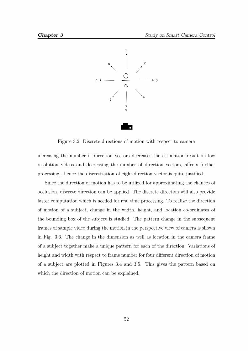
Chapter 3 Study on Smart Camera Control
1
2
3
4
5
6
7
8
Figure 3.2: Discrete directions of motion with respect to camera
increasing the number of direction vectors decreases the estimation result on low
resolution videos and decreasing the number of direction vectors, affects further
processing , hence the discretization of eight direction vector is quite justified.
Since the direction of motion has to be utilized for approximating the chances of
occlusion, discrete direction can be applied. The discrete direction will also provide
faster computation which is needed for real time processing. To realize the direction
of motion of a subject, change in the width, height, and location co-ordinates of
the bounding box of the subject is studied. The pattern change in the subsequent
frames of sample video during the motion in the perspective view of camera is shown
in Fig. 3.3. The change in the dimension as well as location in the camera frame
of a subject together make a unique pattern for each of the direction. Variations of
height and width with respect to frame number for four different direction of motion
of a subject are plotted in Figures 3.4 and 3.5. This gives the pattern based on
which the direction of motion can be explained.
52
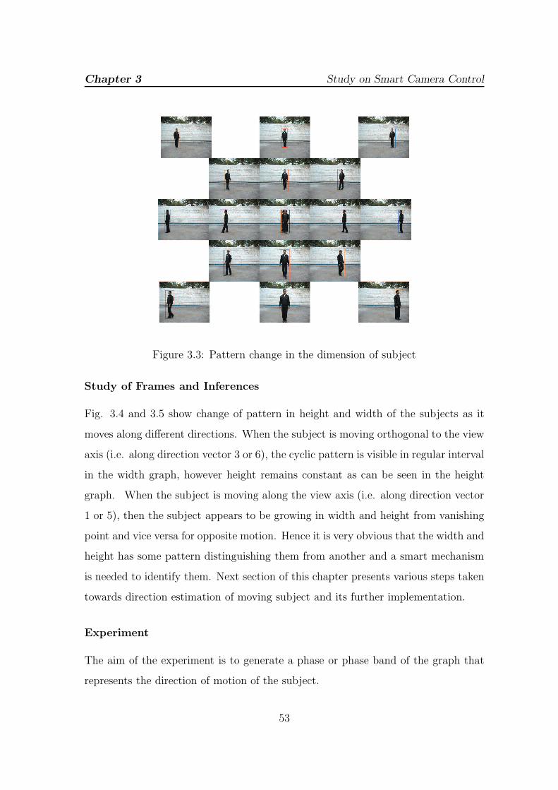
Chapter 3 Study on Smart Camera Control
Figure 3.3: Pattern change in the dimension of subject
Study of Frames and Inferences
Fig. 3.4 and 3.5 show change of pattern in height and width of the subjects as it
moves along different directions. When the subject is moving orthogonal to the view
axis (i.e. along direction vector 3 or 6), the cyclic pattern is visible in regular interval
in the width graph, however height remains constant as can be seen in the height
graph. When the subject is moving along the view axis (i.e. along direction vector
1 or 5), then the subject appears to be growing in width and height from vanishing
point and vice versa for opposite motion. Hence it is very obvious that the width and
height has some pattern distinguishing them from another and a smart mechanism
is needed to identify them. Next section of this chapter presents various steps taken
towards direction estimation of moving subject and its further implementation.
Experiment
The aim of the experiment is to generate a phase or phase band of the graph that
represents the direction of motion of the subject.
53
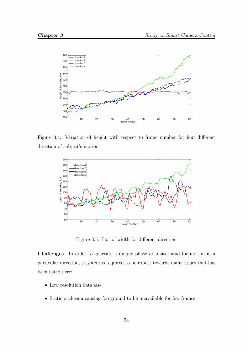
Chapter 3 Study on Smart Camera Control
10 20 30 40 50 60 70 80200
220
240
260
280
300
320
340
360
380
400
Frame Number
Hei
ght o
f Bou
ndin
g B
ox
direction 5direction 6direction 7direction 4
Figure 3.4: Variation of height with respect to frame number for four different
direction of subject’s motion
10 20 30 40 50 60 70 8050
60
70
80
90
100
110
120
130
140
150
160
Frame Number
Wid
th o
f Bou
ndin
g B
ox
direction 4direction 7direction 6direction 5
Figure 3.5: Plot of width for different direction
Challenges In order to generate a unique phase or phase band for motion in a
particular direction, a system is required to be robust towards many issues that has
been listed here:� Low resolution database.� Static occlusion causing foreground to be unavailable for few frames.
54
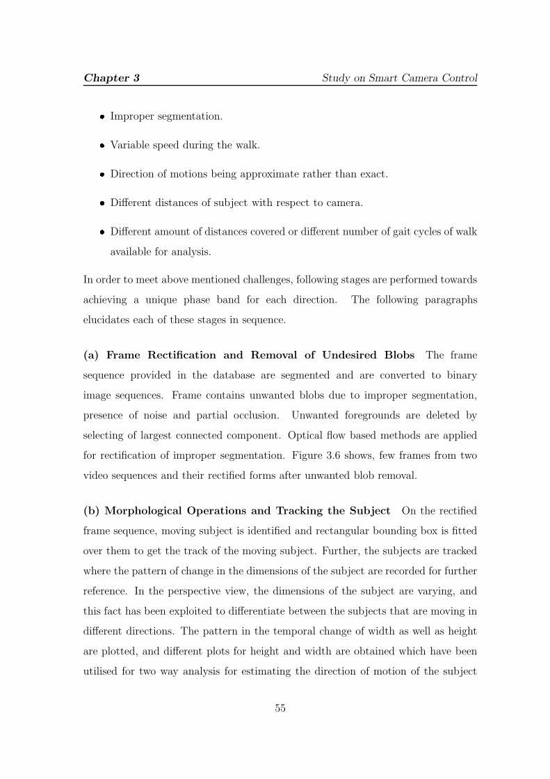
Chapter 3 Study on Smart Camera Control� Improper segmentation.� Variable speed during the walk.� Direction of motions being approximate rather than exact.� Different distances of subject with respect to camera.� Different amount of distances covered or different number of gait cycles of walk
available for analysis.
In order to meet above mentioned challenges, following stages are performed towards
achieving a unique phase band for each direction. The following paragraphs
elucidates each of these stages in sequence.
(a) Frame Rectification and Removal of Undesired Blobs The frame
sequence provided in the database are segmented and are converted to binary
image sequences. Frame contains unwanted blobs due to improper segmentation,
presence of noise and partial occlusion. Unwanted foregrounds are deleted by
selecting of largest connected component. Optical flow based methods are applied
for rectification of improper segmentation. Figure 3.6 shows, few frames from two
video sequences and their rectified forms after unwanted blob removal.
(b) Morphological Operations and Tracking the Subject On the rectified
frame sequence, moving subject is identified and rectangular bounding box is fitted
over them to get the track of the moving subject. Further, the subjects are tracked
where the pattern of change in the dimensions of the subject are recorded for further
reference. In the perspective view, the dimensions of the subject are varying, and
this fact has been exploited to differentiate between the subjects that are moving in
different directions. The pattern in the temporal change of width as well as height
are plotted, and different plots for height and width are obtained which have been
utilised for two way analysis for estimating the direction of motion of the subject
55
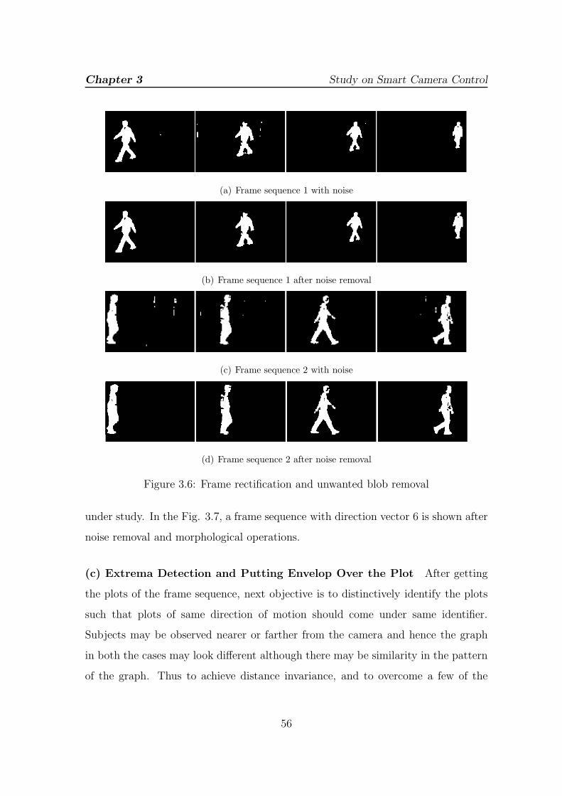
Chapter 3 Study on Smart Camera Control
(a) Frame sequence 1 with noise
(b) Frame sequence 1 after noise removal
(c) Frame sequence 2 with noise
(d) Frame sequence 2 after noise removal
Figure 3.6: Frame rectification and unwanted blob removal
under study. In the Fig. 3.7, a frame sequence with direction vector 6 is shown after
noise removal and morphological operations.
(c) Extrema Detection and Putting Envelop Over the Plot After getting
the plots of the frame sequence, next objective is to distinctively identify the plots
such that plots of same direction of motion should come under same identifier.
Subjects may be observed nearer or farther from the camera and hence the graph
in both the cases may look different although there may be similarity in the pattern
of the graph. Thus to achieve distance invariance, and to overcome a few of the
56
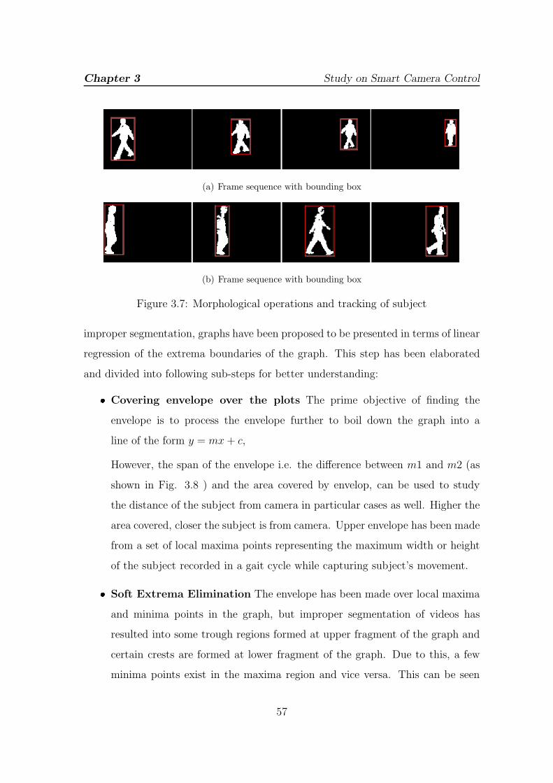
Chapter 3 Study on Smart Camera Control
(a) Frame sequence with bounding box
(b) Frame sequence with bounding box
Figure 3.7: Morphological operations and tracking of subject
improper segmentation, graphs have been proposed to be presented in terms of linear
regression of the extrema boundaries of the graph. This step has been elaborated
and divided into following sub-steps for better understanding:� Covering envelope over the plots The prime objective of finding the
envelope is to process the envelope further to boil down the graph into a
line of the form y = mx+ c,
However, the span of the envelope i.e. the difference between m1 and m2 (as
shown in Fig. 3.8 ) and the area covered by envelop, can be used to study
the distance of the subject from camera in particular cases as well. Higher the
area covered, closer the subject is from camera. Upper envelope has been made
from a set of local maxima points representing the maximum width or height
of the subject recorded in a gait cycle while capturing subject’s movement.� Soft Extrema Elimination The envelope has been made over local maxima
and minima points in the graph, but improper segmentation of videos has
resulted into some trough regions formed at upper fragment of the graph and
certain crests are formed at lower fragment of the graph. Due to this, a few
minima points exist in the maxima region and vice versa. This can be seen
57
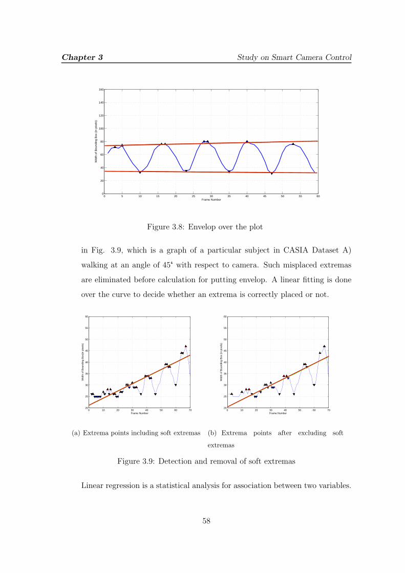
Chapter 3 Study on Smart Camera Control
0 5 10 15 20 25 30 35 40 45 50 55 600
20
40
60
80
100
120
140
160
Frame Number
Wid
th o
f Bou
ndin
g B
ox (
in p
ixel
s)
Figure 3.8: Envelop over the plot
in Fig. 3.9, which is a graph of a particular subject in CASIA Dataset A)
walking at an angle of 45° with respect to camera. Such misplaced extremas
are eliminated before calculation for putting envelop. A linear fitting is done
over the curve to decide whether an extrema is correctly placed or not.
0 10 20 30 40 50 60 7020
25
30
35
40
45
50
55
60
Frame Number
Wid
th o
f Bou
ndin
g B
ox(in
pix
els)
(a) Extrema points including soft extremas
0 10 20 30 40 50 60 7020
25
30
35
40
45
50
55
60
Frame Number
Wid
th o
f Bou
ndin
g B
ox (
in p
ixel
s)
(b) Extrema points after excluding soft
extremas
Figure 3.9: Detection and removal of soft extremas
Linear regression is a statistical analysis for association between two variables.
58
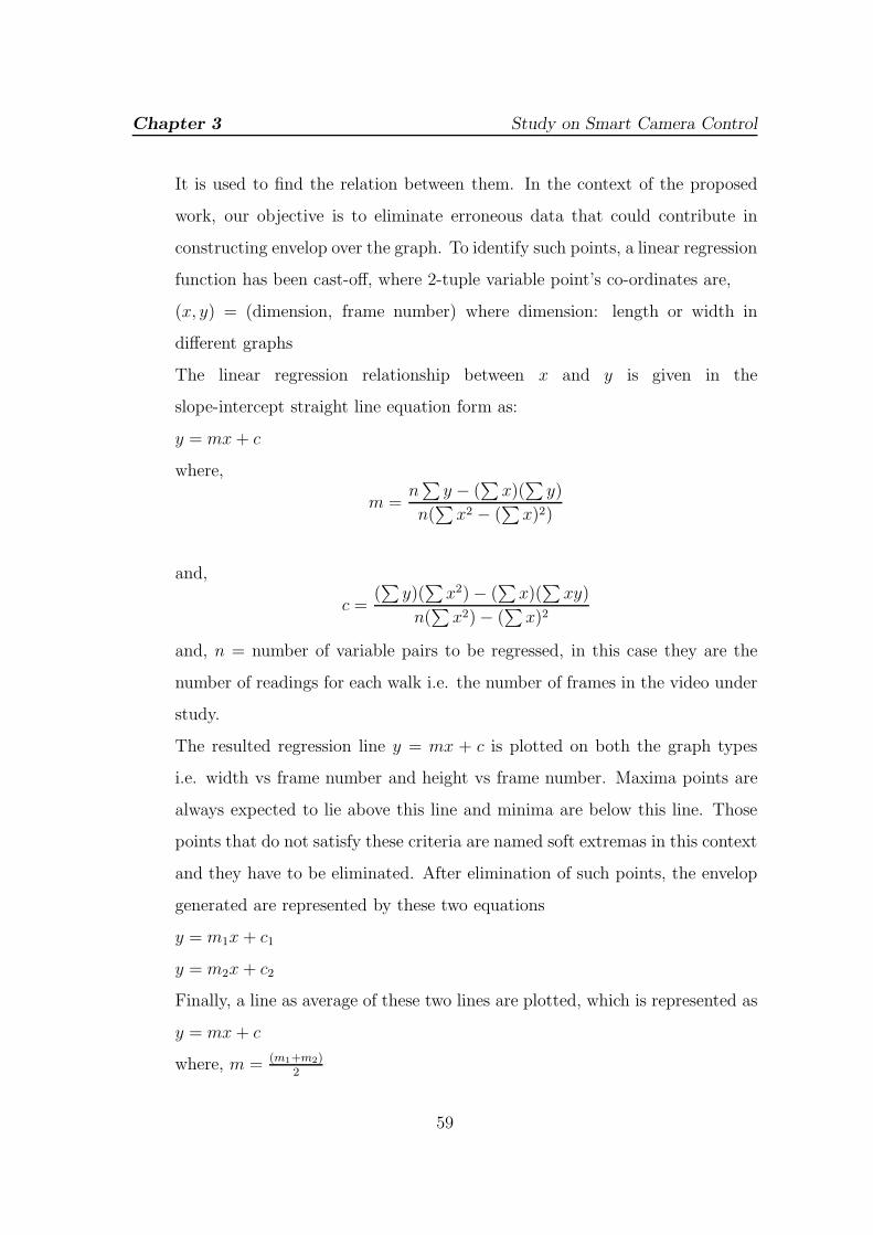
Chapter 3 Study on Smart Camera Control
It is used to find the relation between them. In the context of the proposed
work, our objective is to eliminate erroneous data that could contribute in
constructing envelop over the graph. To identify such points, a linear regression
function has been cast-off, where 2-tuple variable point’s co-ordinates are,
(x, y) = (dimension, frame number) where dimension: length or width in
different graphs
The linear regression relationship between x and y is given in the
slope-intercept straight line equation form as:
y = mx+ c
where,
m =n∑
y − (∑
x)(∑
y)
n(∑
x2 − (∑
x)2)
and,
c =(∑
y)(∑
x2)− (∑
x)(∑
xy)
n(∑
x2)− (∑
x)2
and, n = number of variable pairs to be regressed, in this case they are the
number of readings for each walk i.e. the number of frames in the video under
study.
The resulted regression line y = mx + c is plotted on both the graph types
i.e. width vs frame number and height vs frame number. Maxima points are
always expected to lie above this line and minima are below this line. Those
points that do not satisfy these criteria are named soft extremas in this context
and they have to be eliminated. After elimination of such points, the envelop
generated are represented by these two equations
y = m1x+ c1
y = m2x+ c2
Finally, a line as average of these two lines are plotted, which is represented as
y = mx+ c
where, m = (m1+m2)2
59
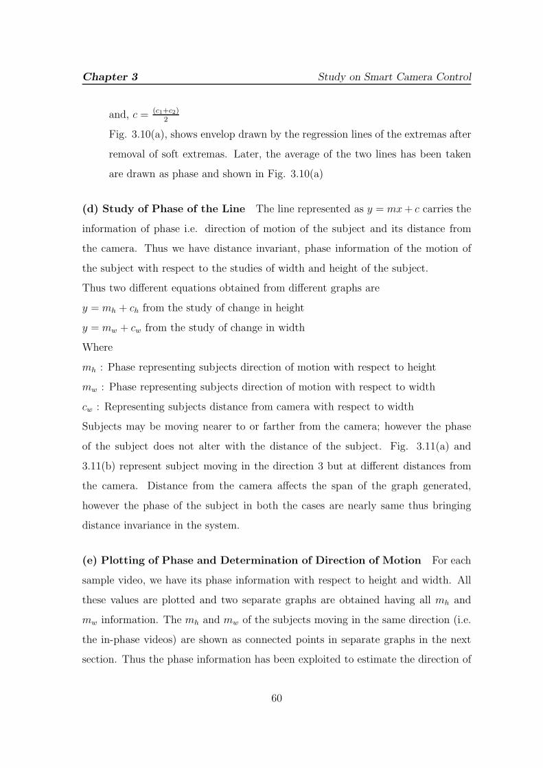
Chapter 3 Study on Smart Camera Control
and, c = (c1+c2)2
Fig. 3.10(a), shows envelop drawn by the regression lines of the extremas after
removal of soft extremas. Later, the average of the two lines has been taken
are drawn as phase and shown in Fig. 3.10(a)
(d) Study of Phase of the Line The line represented as y = mx+ c carries the
information of phase i.e. direction of motion of the subject and its distance from
the camera. Thus we have distance invariant, phase information of the motion of
the subject with respect to the studies of width and height of the subject.
Thus two different equations obtained from different graphs are
y = mh + ch from the study of change in height
y = mw + cw from the study of change in width
Where
mh : Phase representing subjects direction of motion with respect to height
mw : Phase representing subjects direction of motion with respect to width
cw : Representing subjects distance from camera with respect to width
Subjects may be moving nearer to or farther from the camera; however the phase
of the subject does not alter with the distance of the subject. Fig. 3.11(a) and
3.11(b) represent subject moving in the direction 3 but at different distances from
the camera. Distance from the camera affects the span of the graph generated,
however the phase of the subject in both the cases are nearly same thus bringing
distance invariance in the system.
(e) Plotting of Phase and Determination of Direction of Motion For each
sample video, we have its phase information with respect to height and width. All
these values are plotted and two separate graphs are obtained having all mh and
mw information. The mh and mw of the subjects moving in the same direction (i.e.
the in-phase videos) are shown as connected points in separate graphs in the next
section. Thus the phase information has been exploited to estimate the direction of
60
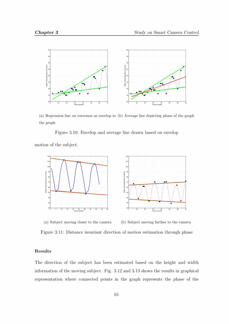
Chapter 3 Study on Smart Camera Control
0 10 20 30 40 50 60 7020
25
30
35
40
45
50
55
60
Frame Number
Wid
th o
f Bou
ndin
g B
ox (
in p
ixel
s)
(a) Regression line on extremas as envelop to
the graph
0 10 20 30 40 50 60 7020
25
30
35
40
45
50
55
60
Frame Number
Wid
th o
f Bou
ndin
g B
ox (
in p
ixel
s)
(b) Average line depicting phase of the graph
Figure 3.10: Envelop and average line drawn based on envelop
motion of the subject.
0 5 10 15 20 25 30 35 40 45 5020
30
40
50
60
70
80
90
100
110
120
Frame Number
Wid
th o
f Bou
ndin
g B
ox (
in P
ixel
s)
(a) Subject moving closer to the camera
0 10 20 30 40 50 60 7020
30
40
50
60
70
80
90
100
110
120
Frame Number
Wid
th o
f Bou
ndin
g B
ox (
in p
ixel
s)
(b) Subject moving farther to the camera
Figure 3.11: Distance invariant direction of motion estimation through phase
Results
The direction of the subject has been estimated based on the height and width
information of the moving subject. Fig. 3.12 and 3.13 shows the results in graphical
representation where connected points in the graph represents the phase of the
61
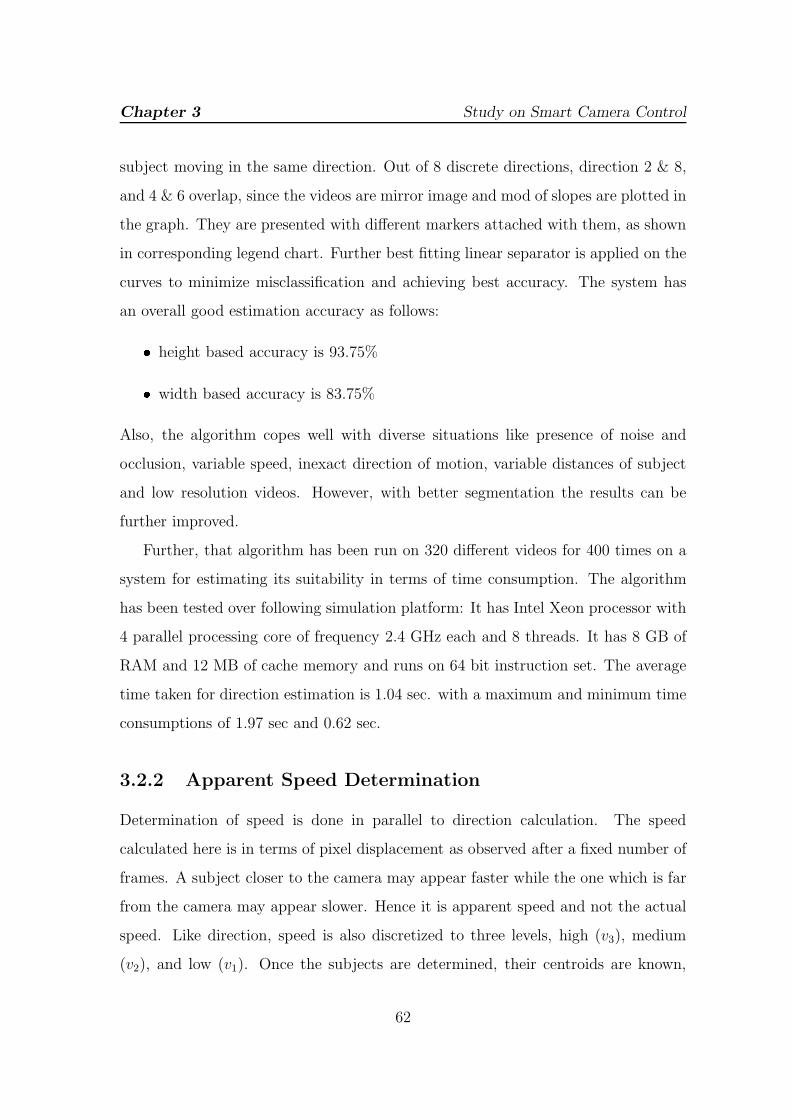
Chapter 3 Study on Smart Camera Control
subject moving in the same direction. Out of 8 discrete directions, direction 2 & 8,
and 4 & 6 overlap, since the videos are mirror image and mod of slopes are plotted in
the graph. They are presented with different markers attached with them, as shown
in corresponding legend chart. Further best fitting linear separator is applied on the
curves to minimize misclassification and achieving best accuracy. The system has
an overall good estimation accuracy as follows:� height based accuracy is 93.75%� width based accuracy is 83.75%
Also, the algorithm copes well with diverse situations like presence of noise and
occlusion, variable speed, inexact direction of motion, variable distances of subject
and low resolution videos. However, with better segmentation the results can be
further improved.
Further, that algorithm has been run on 320 different videos for 400 times on a
system for estimating its suitability in terms of time consumption. The algorithm
has been tested over following simulation platform: It has Intel Xeon processor with
4 parallel processing core of frequency 2.4 GHz each and 8 threads. It has 8 GB of
RAM and 12 MB of cache memory and runs on 64 bit instruction set. The average
time taken for direction estimation is 1.04 sec. with a maximum and minimum time
consumptions of 1.97 sec and 0.62 sec.
3.2.2 Apparent Speed Determination
Determination of speed is done in parallel to direction calculation. The speed
calculated here is in terms of pixel displacement as observed after a fixed number of
frames. A subject closer to the camera may appear faster while the one which is far
from the camera may appear slower. Hence it is apparent speed and not the actual
speed. Like direction, speed is also discretized to three levels, high (v3), medium
(v2), and low (v1). Once the subjects are determined, their centroids are known,
62
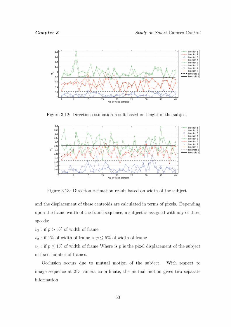
Chapter 3 Study on Smart Camera Control
1 5 10 15 20 25 30 35 400
0.2
0.4
0.6
0.8
1
1.2
1.4
1.6
1.8
No. of video samples
mh
direction 1direction 2direction 3direction 4direction 5direction 6direction 7direction 8threshold 1threshold 2
Figure 3.12: Direction estimation result based on height of the subject
0 5 10 15 20 25 30 35 400
0.05
0.1
0.15
0.2
0.25
0.3
0.35
0.4
0.45
0.5
0.55
0.60.6
No. of video samples
mw
direction 1direction 2direction 3direction 4direction 5direction 6direction 7direction 8threshold 1threshold 2
Figure 3.13: Direction estimation result based on width of the subject
and the displacement of these centroids are calculated in terms of pixels. Depending
upon the frame width of the frame sequence, a subject is assigned with any of these
speeds:
v3 : if p > 5% of width of frame
v2 : if 1% of width of frame < p ≤ 5% of width of frame
v1 : if p ≤ 1% of width of frame Where is p is the pixel displacement of the subject
in fixed number of frames.
Occlusion occurs due to mutual motion of the subject. With respect to
image sequence at 2D camera co-ordinate, the mutual motion gives two separate
information
63
Chapter 3 Study on Smart Camera Control� Change in the dimension of the subject, that eventually gives the direction of
motion of subject� Change in the location of subject that gives the speed and present location of
the subject
Both of these information are already estimated by the approaches proposed in
the earlier section. Next section describes the application of these information in
determining the proximity of occlusion.
3.3 Occlusion Determination
Successful calculation of direction and apparent speed of a moving subject takes the
work to the next level where based on the above results, chances of occlusion of a
subject is determined. The direction of motion and speed informations are used in
lookup table generation. Further, based on the lookup table chances of occlusion
and its location and time to occlusion are calculated. This section presents some
pre-calculations, and steps for developing lookup table. Once the lookup table is
generated, it can be referenced for determination of chances of occlusion, and in
cases of occlusion determination of time and position of occlusion in camera frame.
Further, related calculations are presented in this section.
Pre-calculations : Given the first f frames
* Locations: Centroid of both the subjects Sp and Sq represented as their
locations as
L(Sp) : (xp, yp)
L(Sq) : (xq, yq).
* Deciding S1 and S2 : With the location information of both the subjects,
the one with lesser abscissa is said to be Subject 1 (S1) and the other subject
becomes Subject 2 (S2). This has been described in the algorithm 1.
64
Chapter 3 Study on Smart Camera Control
* Distance: Apparent distance between the subjects can be calculated in terms
of pixels as
d =√
(x2 − x1)2 + (y2 − y1)2
* Directions: Direction of a subject S1
given by D(S1) is the discrete direction of a subject as determined in the
Section 3.2.1
Such that,
D(S1) ∈ {1, 2, 3, 4, 5, 6, 7, 8}
D(S2) ∈ {1, 2, 3, 4, 5, 6, 7, 8}
* Speeds: In the first f input frames, the pixel displacement of the subject’s
centroid gives apparent speed of the subject, which is categorized to three
levels as fast (V3), medium (V2) and slow (V1). This has been discussed in
Section 3.2.2. The speed is in terms of pixel displacement in f frames and
while calculations in the next section, V (S1) and V (S2) are presented as p1
and p2 respectively.
Such that,
V (S1) ∈ {V1, V2, V3}
V (S2) ∈ {V1, V2, V3}
3.3.1 Lookup table generation
The direction of mutual motion of the subjects mostly determines the chances of
occlusion, hence estimation is not only dependent on 8 discrete directions of a subject
but on the mutual combinations of motion of the subject. Hence, chances of occlusion
due to direction of motion of any pair of potential occluder are best represented
with an 8 × 8 matrix. Further, with each pair of direction of the subjects their
65
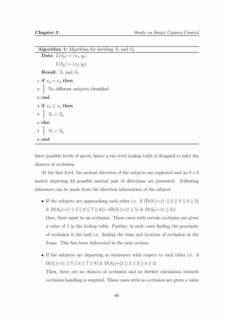
Chapter 3 Study on Smart Camera Control
Algorithm 1: Algorithm for deciding S1 and S2
Data: L(Sp) = (xp, yp)
L(Sq) = (xq, yq)
Result: S1 and S2
1 if xp = xq then
2 No different subjects identified
3 end
4 if xp ≤ xq then
5 S1 = Sp
6 else
7 S1 = Sq
8 end
three possible levels of speed, hence a two level lookup table is designed to infer the
chances of occlusion.
At the first level, the mutual direction of the subjects are exploited and an 8× 8
matrix depicting 64 possible mutual pair of directions are presented. Following
inferences can be made from the direction information of the subject:� If the subjects are approaching each other i.e. if (D(S1)=(1 || 2 || 3 || 4 || 5)
& D(S2)=(1 || 5 || 6 || 7 || 8))−(D(S1)=(1 || 5) & D(S2)=(1 || 5))
then, there must be an occlusion. These cases with certain occlusion are given
a value of 1 in the lookup table. Further, in such cases finding the proximity
of occlusion is the task i.e. finding the time and location of occlusion in the
frame. This has been elaborated in the next section.� If the subjects are departing or stationary with respect to each other i.e. if
D(S1)=(1 || 5 || 6 || 7 || 8) & D(S2)=(1 || 2 || 3 || 4 || 5)
Then, there are no chances of occlusion and no further calculation towards
occlusion handling is required. These cases with no occlusion are given a value
66
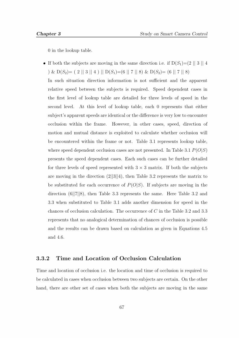
Chapter 3 Study on Smart Camera Control
0 in the lookup table.� If both the subjects are moving in the same direction i.e. if D(S1)=(2 || 3 || 4
) & D(S2)= ( 2 || 3 || 4 ) || D(S1)=(6 || 7 || 8) & D(S2)= (6 || 7 || 8)
In such situation direction information is not sufficient and the apparent
relative speed between the subjects is required. Speed dependent cases in
the first level of lookup table are detailed for three levels of speed in the
second level. At this level of lookup table, each 0 represents that either
subject’s apparent speeds are identical or the difference is very low to encounter
occlusion within the frame. However, in other cases, speed, direction of
motion and mutual distance is exploited to calculate whether occlusion will
be encountered within the frame or not. Table 3.1 represents lookup table,
where speed dependent occlusion cases are not presented. In Table 3.1 P (O|S)
presents the speed dependent cases. Each such cases can be further detailed
for three levels of speed represented with 3 × 3 matrix. If both the subjects
are moving in the direction (2||3||4), then Table 3.2 represents the matrix to
be substituted for each occurrence of P (O|S). If subjects are moving in the
direction (6||7||8), then Table 3.3 represents the same. Here Table 3.2 and
3.3 when substituted to Table 3.1 adds another dimension for speed in the
chances of occlusion calculation. The occurrence of C in the Table 3.2 and 3.3
represents that no analogical determination of chances of occlusion is possible
and the results can be drawn based on calculation as given in Equations 4.5
and 4.6.
3.3.2 Time and Location of Occlusion Calculation
Time and location of occlusion i.e. the location and time of occlusion is required to
be calculated in cases when occlusion between two subjects are certain. On the other
hand, there are other set of cases when both the subjects are moving in the same
67
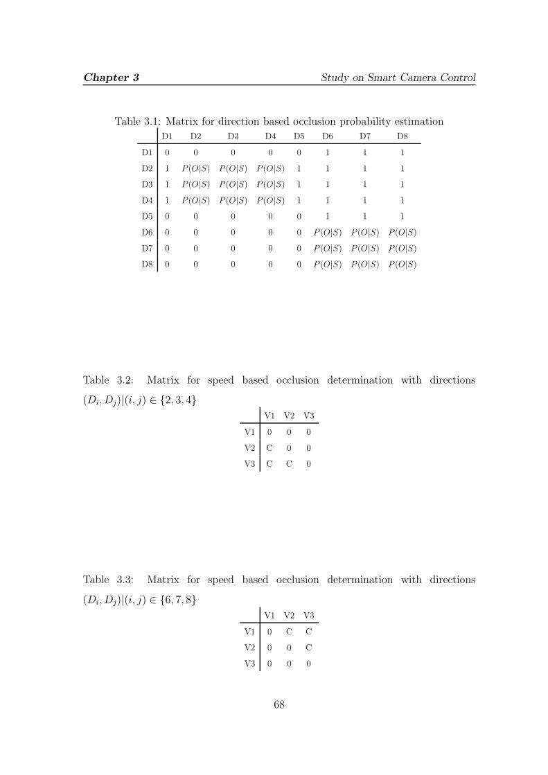
Chapter 3 Study on Smart Camera Control
Table 3.1: Matrix for direction based occlusion probability estimation
D1 D2 D3 D4 D5 D6 D7 D8
D1 0 0 0 0 0 1 1 1
D2 1 P (O|S) P (O|S) P (O|S) 1 1 1 1
D3 1 P (O|S) P (O|S) P (O|S) 1 1 1 1
D4 1 P (O|S) P (O|S) P (O|S) 1 1 1 1
D5 0 0 0 0 0 1 1 1
D6 0 0 0 0 0 P (O|S) P (O|S) P (O|S)
D7 0 0 0 0 0 P (O|S) P (O|S) P (O|S)
D8 0 0 0 0 0 P (O|S) P (O|S) P (O|S)
Table 3.2: Matrix for speed based occlusion determination with directions
(Di, Dj)|(i, j) ∈ {2, 3, 4}
V1 V2 V3
V1 0 0 0
V2 C 0 0
V3 C C 0
Table 3.3: Matrix for speed based occlusion determination with directions
(Di, Dj)|(i, j) ∈ {6, 7, 8}
V1 V2 V3
V1 0 C C
V2 0 0 C
V3 0 0 0
68
Chapter 3 Study on Smart Camera Control
direction and whether their occlusion will be encountered in the current camera or
not is the issue. This section discusses the calculation involved in both the cases one
by one.
When the subjects are approaching each other Motion analysis of the
subject determines the direction of their movement, based on which lookup table
has been generated that indicates the chances of occlusion. If the subjects are found
to be approaching towards each other, then the occlusion is certain and next task is
to calculate its proximity i.e. its time and location of encountering occlusion. Let
p1 : apparent speed of S1
i.e. p1 pixels travelled in f frames (1 second)
p2 : apparent speed of S2
i.e. p2 pixels travelled in f frames (1 second)
if subjects are approaching each other
then, relative speed between subjects=(p1 + p2)
i.e.(p1 + p2) pixels would be covered in f frames
then, d pixels would be covered in dp1+p2
seconds
therefore time to occlusion is given by
d
p1 + p2(3.1)
and, frame number of occlusion is given by ( dp1+p2
)× f
if (x, y) be the point of occlusion, then
equating the distance equation between two points and distance as product of time
and speed
(dp1
p1 + p2)2 = (D1)
2 = (x− x1)2 + (y − y1)
2 (3.2)
(dp2
p1 + p2)2 = (D2)
2 = (x− x2)2 + (y − y2)
2 (3.3)
69
Chapter 3 Study on Smart Camera Control
also, considering the relation between (x, y) and (x1, y1)
(y − y1)
(x− x1)= m (3.4)
where m being the slope of motion direction of S1
Using Equations 3.2,3.3 and 3.4, the location of occlusion is given by
x =2(mx1 − y1)(y1 − y2)− ((D1)
2 − (D2)2) + ((x1)
2 − (x2)2) + ((y1)
2 − (y2)2)
2m(y1 − y2) + 2(x1 − x2)(3.5)
and
y = −mx1 + y1 +mx (3.6)
The apparent location of occlusion is thus given by (x,y).
When the subjects are moving in the same direction Direction of motion
of the subjects are not sufficient to determine the chances of occlusion in some
cases. These are the cases when both the subjects are moving in the same direction
and any chance of occlusion depends upon the relative speed between the subjects.
Considering the same variables if subjects are departing each other,
relative speed between subjects=(|p1 − p2|)
d pixels would be covered in d|p1−p2|
seconds
Now, using same distance Equations 3.2, 3.3 and 3.4, the co-ordinates of location
of occlusion can be determined. However, in this case if the co-ordinates (x, y)
are within the frame range, then occlusion will be encountered in the view of this
camera, otherwise no occlusion will be observed.
70
Chapter 3 Study on Smart Camera Control
3.4 Mitigation of Occlusion
Based on the direction of motion and speed of the subjects, their probability and
proximity of occlusion are determined. Up to this level, the system acts as a single
camera system. After a conclusion is drawn about the proximity of occlusion, then
steps towards mitigation of occlusion takes place. Multiple cameras in the systems
are precalibrated and localized. Hence the poses of cameras are known to each
other. In case of any possible occlusion, the active camera selects minimal number
of cameras in the network that is not expected to encounter occlusion at the same
time. This camera will awake those set of cameras and they start further tracking
of subject. This will not only let the continuous tracking of subjects possible but
also let the cameras to work efficiently in terms of energy and avoids processing
complexity.
To justify the proposed approach towards occlusion determination, different cases
are experimented. Sample videos are captured with various possible motions in
different directions depicting the scenario of occlusion and non-occlusion. CASIA
Dataset A database which contains gait pattern of different subjects and captured
from different camera angles are modified to get eight different directions of motion
and are added in such a way to get variety of cases of occlusion. During the motion,
subject may be nearer to or far from the camera and hence may appear larger or
smaller in size, but the characteristics of the graph remains unchanged irrespective
of its appearance (as seen in the Fig.3.11). The next section presents various cases of
encountering occlusion and the cases of non occlusion observed over CASIA database
as well as self acquired database.
3.5 Results
The earlier sections of this chapter presents our novel approach towards achieving
uninterrupted track of the subject in an MCN environment that optimally utilises
71
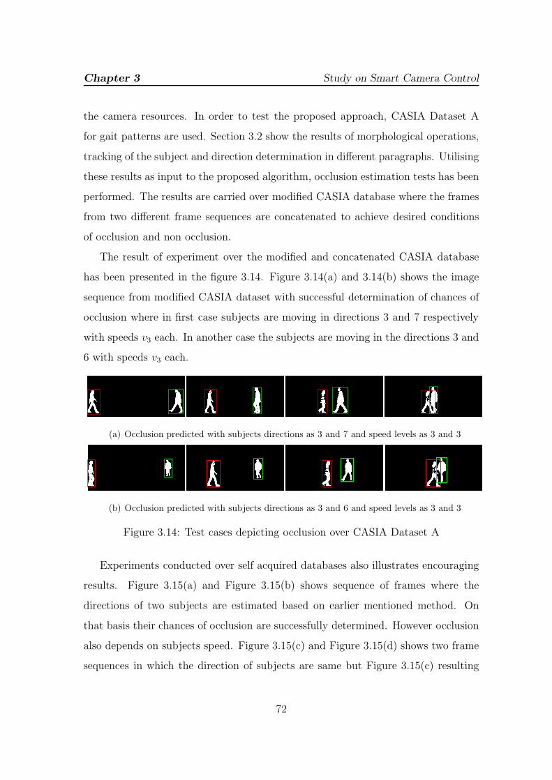
Chapter 3 Study on Smart Camera Control
the camera resources. In order to test the proposed approach, CASIA Dataset A
for gait patterns are used. Section 3.2 show the results of morphological operations,
tracking of the subject and direction determination in different paragraphs. Utilising
these results as input to the proposed algorithm, occlusion estimation tests has been
performed. The results are carried over modified CASIA database where the frames
from two different frame sequences are concatenated to achieve desired conditions
of occlusion and non occlusion.
The result of experiment over the modified and concatenated CASIA database
has been presented in the figure 3.14. Figure 3.14(a) and 3.14(b) shows the image
sequence from modified CASIA dataset with successful determination of chances of
occlusion where in first case subjects are moving in directions 3 and 7 respectively
with speeds v3 each. In another case the subjects are moving in the directions 3 and
6 with speeds v3 each.
(a) Occlusion predicted with subjects directions as 3 and 7 and speed levels as 3 and 3
(b) Occlusion predicted with subjects directions as 3 and 6 and speed levels as 3 and 3
Figure 3.14: Test cases depicting occlusion over CASIA Dataset A
Experiments conducted over self acquired databases also illustrates encouraging
results. Figure 3.15(a) and Figure 3.15(b) shows sequence of frames where the
directions of two subjects are estimated based on earlier mentioned method. On
that basis their chances of occlusion are successfully determined. However occlusion
also depends on subjects speed. Figure 3.15(c) and Figure 3.15(d) shows two frame
sequences in which the direction of subjects are same but Figure 3.15(c) resulting
72

Chapter 3 Study on Smart Camera Control
occlusion while Figure 3.15(d) avoids occlusion. The direction in both the cases is
found to be direction 3. The difference in the subject’s speed level is found zero in
Figure 3.15(c) resulting non-occlusion while the speed level difference is found to be
two in Figure 3.15(d) resulting occlusion.
(a) Occlusion predicted with subjects directions as 2 and 6
(b) Occlusion predicted with subjects directions as 3 and 7
(c) Occlusion predicted with subjects directions as 3 and 3 but speed levels as 3 and 1
(d) No occlusion predicted with subjects directions as 3 and 3 but speed levels as 1 and 1
Figure 3.15: Test cases depicting occlusion and non occlusion
3.6 Concluding Remarks
The proposed work shows efficient and effective way for determining occlusion and
avoiding it in a multi-camera network. The proposed camera network works in single
camera mode avoiding complexity and higher operation cost as long as tracking is
73

Chapter 3 Study on Smart Camera Control
possible from one camera. It awake one or more cameras in case of any occlusion and
does not compromise in losing the track of the subject. It finds its implementation
in places like dedicated roads, office corridor, passage in railway station, airports,
subways, shopping malls and other places where multiple cameras can be installed.
74

Chapter 4
Conclusion
With ever increasing demand of surveillance and rapidly advancing camera
technology, mankind has landed into the era of visual surveillance. Over the time,
dependency and necessity over visual surveillance is growing rapidly and so is the
research in the domain. The tracking and recognition over single camera has been
elaborated and the multi-camera network (MCN) has emerged as a solution to
overcome the limitations of single camera-based visual surveillance. This thesis
explores the trade-offs of single as well as multi-camera based surveillance and
attempts to optimize multi-camera set-up as in single camera system yet not
compromising the benefits of multi-camera based surveillance system.
With different chapters, different levels of multi-camera development model have
been explored, and survey, proposals, experiments and results are presented that
lead to a model for an efficient surveillance system.
The necessity and advancement of calibration and localization of multi-camera
network has been studied and presented in chapter 1. The chapter elaborates
the complexity as well as necessity of a calibrated multi-camera network. The
chapter explores different research challenges in the domain of multi-camera network.
Effective utilization of camera is a major issue in MCN, this has been resolved
with research on effective placement of camera. Chapter 2 discusses various camera
75
Conclusion
placement techniques and presents a novel approach towards task specific efficient
placement of field cameras in the proposed model. With the aim of capturing gait
patterns of moving subjects, a novel camera placement technique has been proposed
that places the camera so as to stay orthogonal to the direction of movement of
the subject. The proposed model has been experimentally tested over a corridor
sequence taken at Vikram Sarabhai Hall of Residence at NIT Rourkela and based
on the number of walks of different subjects, suitable camera placement results are
presented. With cameras placed efficiently, the camera control is also an important
issue in MCN based surveillance. Chapter 3 presents research on camera control. To
justify the scope of the model, a brief comparison of single and multi-camera based
surveillance and their benefits and trade-offs are presented in chapter 1. A three
step model has been proposed that lets most of the cameras to stay in sleep mode
while minimal cameras are tracking the subject. Direction and apparent speed of the
subjects are determined and with their results, chances of occlusion are calculated.
In case of any chances of occlusion, the time and placement of occlusion is also
determined. A prior knowledge of occlusion will let the system to take necessary
action towards mitigation of occlusion. These experiments are performed on existing
database, CASIA Dataset A for gait and its modified versions.
Scope for future research
The experiment conducted towards the proposed model has produced motivating
results. It achieves good accuracy in challenging situations as� Changing speed of the subject within video.� Different velocity of subject in different video.� Different distances of the subject from the camera.� Presence of noise and partial occlusion.
76
Conclusion� Direction of motion of subject being not accurate.� Varying direction of subject while motion.� Low resolution video.
Many challenges have been identified and expected. Even though ample
justification has been given towards the efficient placement of camera work, and
experimental results over self acquired data has been produced, it still awaits
experimental justification in complex surveillance zone. Further scope towards
implementation of the proposed work lies in developing algorithms that can decide
the control flow from one camera to another. Mitigation of occlusion can be done
when a robust algorithm can utilize the pose (position with orientation) information
of pre-localized and calibrated cameras, and based on these values, it can awake the
camera which does not encounter occlusion at all. Since the algorithm works in real
time environment and finds its implementation in vital issue as surveillance, fast
and optimized working along with high accuracy is a concern that can always be
explored.
77
Bibliography
[1] P. Kulkarni, D. Ganesan, and P. Shenoy. The case for multi–tier camera sensor networks.
In Proceedings of the international workshop on Network and operating systems support for
digital audio and video, NOSSDAV, pages 141–146, 2005.
[2] P. Kulkarni, D. Ganesan, P. Shenoy, and Q. Lu. Senseye: a multi-tier camera sensor
network. In Proceedings of the 13th annual ACM international conference on Multimedia,
pages 229–238, 2005.
[3] Hartley R. and Zisserman A. Multiple view geometry in computer vision. Cambridge Univ.
Press, 2 edition, 2004.
[4] Davis L., Borovikov E., Cutler R., Harwood D., and Horprasert T. Multi-perspective analysis
of human action. In Proceedings of 3rd International Workshop on Cooperative Distributed
Vision, Kyoto, Japan, 1999.
[5] Kanade T., Rander P., and Narayanan P.J. Virtualized reality: Constructing virtual worlds
from real scenes. 4(1):34–47, 1997.
[6] Piovan G., Shames I., Fidan B., Bullo F., and Anderson B.D.O. On frame and orientation
localization for relative sensing networks. In 47th IEEE Conference on Decision and Control,
CDC08, pages 2326–2331. IEEE, 2008.
[7] Taylor C., Rahimi A., Bachrach J., Shrobe H., and Grue A . Simultaneous localization,
calibration, and tracking in an ad hoc sensor network. In 5th International Conference on
Information Processing in Sensor Networks, IPSN. ACM, 2006.
[8] Aspnes J., Eren T., Goldenberg D.K., Morse A.S., Whiteley W., Yang Y.R., Anderson
B.D.O., and Balhumeur P. A theory of network localization. IEEE Transactions on Mobile
Computing, 5(12):1663–1678, 2006.
[9] Eren T., Goldenberg D.K., Whiteley W., Yang Y.R., Morse A.S., Anderson B.D.O., and
Belhumeur P.N. Rigidity, computation, and randomization in network localization. In
Proceedings of 23rd Annual Joint Conference of the IEEE Computer and Communications
Societies, volume 4 of INFOCOM, 2004.
78
Bibliography
[10] Biswas P. and Ye Y. Semidefinite programming for ad hoc wireless sensor network
localization. In 3rd international symposium on Information processing in sensor networks,
IPSN 2004, pages 46–54. ACM, 2004.
[11] Funiak S., Guestrin C., Paskin M., and Sukthankar R. Distributed localization of networked
cameras. In 5th International Conference on Information Processing in Sensor Networks,
IPSN, pages 34–42. ACM, 2006.
[12] Liu X., Kulkarni P., and Shenoy P. Snapshot: a self-calibration protocol for camera sensor
networks. In 3rd International Conference on Broadband Communications, Networks, and
Systems, BROADNETS, 2006.
[13] Mantzel W. E., Choi H., and Baraniuk R. G. Distributed camera network localization. In
38th Asilomar Conference on Signals, Systems and Computers, volume 2, pages 1381–1386,
2004.
[14] Devarajan D. and Radke R. Calibrating distributed camera networks using belief
propagation. EURASIP Journal of Applied Signal Processing, 2007.
[15] Tron R., Vidal R., and Terzis A. Distributed pose averaging in camera networks via consensus
on se(3). In 2nd ACM/IEEE International Conference on Distributed Smart Cameras,
ICDSC. ACM/IEEE, 2008.
[16] Bondy J. A. and Murty U. S. R. Graph theory with applications. Elsevier Science Publishing
Co., 1982.
[17] Kurillo G., Li Z., and Bajcsy R. Wide-area external multi-camera calibration using vision
graphs and virtual calibration object. In 2nd ACM/IEEE International Conference on
Distributed Smart Cameras, ICDSC, pages 85–94. ACM, 2008.
[18] Lowe D.G. Distinctive image features from scale-invariant keypoints. 60(2), 2004.
[19] Lymberopoulos D., Sweeny A. B., and Savvides A. Sensor localization and camera calibration
using low power cameras. In ENALAB Technical Report. 090105, 2004.
[20] Medeiros H., Iwaki H., and Park J. Online distributed calibration of a large network of
wireless cameras using dynamic clustering. In 2nd ACM/IEEE International Conference on
Distributed Smart Cameras, volume 2 of ICDSC, pages 1381–1386. ACM/IEEE, 2008.
[21] Ellis T.J., Makris D., and Black J. Learning a multicamera topology. In IEEE International
Workshop on Visual Surveillance & Performance Evaluation of Tracking & Surveillance,
pages 165–171, 2003.
79

Bibliography
[22] Marinakis D., Dudek G., and Fleet D. Learning sensor network topology through monte carlo
expectation maximisation. In IEEE International Conference on Robotics & Automation,
2005.
[23] Rahimi A., Dunagan B., and Darrell T. Simultaneous calibration and tracking with a network
of non-overlapping sensors. In IEEE Computer Society Conference on Computer Vision and
Pattern Recognition, volume 1 of CVPR, pages I–187–I–194. IEEE, 2004.
[24] Barton-Sweeney A., Lymberopoulos D., and Sawides A. Sensor localization and camera
calibration in distributed camera sensor networks. In 3rd International Conference on
Broadband Communications, Networks and Systems, BROADNETS, 2006.
[25] Farrell R., Garcia R., Lucarelli D., Terzis A., and Wang I.J. Localization in multi-modal
sensor networks. 3rd International Conference on Intelligent Sensors, Sensor Networks and
Information (ISSNIP), pages 37–42, 2007.
[26] Goldenberg D.K., Krishnamurthy A., Maness W.C., Yang Y.R., Young A., Morse A.S.,
and Savvides A. Network localization in partially localizable networks. In 24th Annual
Joint Conference of the IEEE Computer and Communications Societies, INFOCOM, pages
313–326. IEEE, 2005.
[27] Sturm P.F. and Triggs B. A factorization based algorithm for multi-image projective structure
and motion. In 4th European Conference on Computer Vision ECCV ’96, volume 2 of ECCV
’96, pages 709–720. Springer-Verlag, 1996.
[28] Nakazato Y., Kanbara M., and Yokoya N. Localization of wearable users using invisible
retro-reflective markers and an ir camera. In Electronic Imaging, SPIE, pages 1234–1242,
2005.
[29] Nakazato Y., Kanbara M., and Yokoya N. A localization system using invisible retro-reflective
markers. In IAPR Conference on Machine Vision Applications, IAPR, pages 140–143, 2005.
[30] Tenmoku R., Kanbara M., and Nakazato Y. Augmented reality system using positioning
infrastructures and a pedometer. In 7th IEEE International Symposium on Wearable
Computers, pages 110–117. IEEE computer Society, 2003.
[31] Maeda M., Ogawa T., Kiyokawa K., and Takemura H. Tracking of user position and
orientation by stereo measurement of infrared markers and orientation sensing. In 8th IEEE
International Symposium on Wearable Computers. IEEE, 2004.
[32] Kato H. and Billinghurst M. Marker tracking and hmd calibration for a video-based
augmented reality conferencing system. In 2nd IEEE and ACM International Workshop
on Augmented Reality, number 10 in IWAR, pages 85–94. IEEE, 1999.
80
Bibliography
[33] Chum O., Matas J., and Obdrzalek S. Epipolar geometry from three correspondences.
CVWW. 2003.
[34] Zhang Z. Determining the epipolar geometry and its uncertainty: A review. International
Journal of Computer Vision, 27(2):161–195, 1998.
[35] Ma Y., Soatto S., Kosecka J., and Sastry S.S. An invitation to 3d vision: From images to
geometric models. In Interdisciplinary Applied Mathematics, volume 26. Springer, 2004.
[36] Liu Y., Huang T.S., and Faugeras O.D. Determination of camera location from 2-d to 3-d
line and point correspondences. 12(1):28–37, 1990.
[37] Xu G. and Zhang Z. In Epipolar geometry in stereo, motion and object recognition: A unified
approach. Springer, 1996.
[38] Spurlock S. and Souvenir R. Dynamic subset selection for multi-camera tracking. In 50th
Annual Southeast Regional Conference. ACM, 2012.
[39] Taj M. and Cavallaro A. Distributed and decentralized multicamera tracking. In Signal
Processing Magazine, IEEE, volume 28, pages 46–58. IEEE, 2011.
[40] Bulusu N., Heidemann J., and Estrin D. Gps-less low-cost outdoor localization for very small
devices. Personal Communications, 7(5):28–34, 2000.
[41] Taylor C.J. A scheme for calibrating smart camera networks using active lights. In 2nd
international conference on Embedded networked sensor systems, SenSys 04, pages 322–322.
ACM, 2004.
[42] Devarajan D., Radke R.J., and Chung H. Distributed metric calibration of ad hoc camera
networks. ACM Transactions on Sensor Networks, 2(3):380–403, 2006.
[43] Kassebaum J., Bulusu N., and Feng W. 3-d target-based distributed smart camera network
localization. (10):2530–2539, 2010.
[44] Olfati-Saber R., Fax J.A., and Murray R.M. Consensus and cooperation in networked
multi-agent systems. In in Proceedings of the IEEE, pages 215–233, 2007.
[45] Gotsman C. and Koren Y. Distributed graph layout for sensor networks. In International
Symposium on Graph Drawing, pages 273–284, 2004.
[46] Khan U.A., Kar S., and Moura J.M.F. Distributed sensor localization in random
environments using minimal number of anchor nodes. IEEE Transactions on Signal
Processing, 57(5), 2009.
81
Bibliography
[47] Tron R. and Vidal R. Distributed image-based 3d localization of camera sensor networks. In
48th IEEE Conference on Decision and Control. IEEE, 2009.
[48] Isard M. and Blake A. Condensation - conditional density propagation for visual tracking.
In Computer Vision, volume 29, 1998.
[49] Freeman W.T. and Pasztor E.C. Learning low-level vision. 7th IEEE International
Conference on Computer Vision, 2, 1999.
[50] Coughlan J.M. and Ferreira S.J. Finding deformable shapes using loopy belief propagation.
In Proceedings of 7th European Conference on Computer Vision - Part III, ECCV ’02, pages
453–468, London, UK, 2002. Springer-Verlag.
[51] Felzenszwalb P.F. and Huttenlocher D.R. Efficient belief propagation for early vision. In 2004
IEEE Computer Society Conference on Computer Vision and Pattern Recognition, volume 1
of CVPR, 2004.
[52] Sudderth E.B., Mandel M.I., Freeman W.T., and Willsky A.S. Distributed occlusion
reasoning for tracking with nonparametric belief propagation. In Advances in Neural
Information Processing Systems, volume 17. MIT Press, 2005.
[53] Murphy K.P., Weiss Y., and Jordan M.I. Loopy belief propagation for approximate inference:
an imperical study. In Uncertainty in Artificial Intelligence, UAI, pages 467–475, 1999.
[54] Pearl J. In Probabilistic reasoning in intelligent systems: Networks of plausible inference.
Morgan Kaufmann Publishers Inc, 1988.
[55] Paskin M.A. and Guestrin C.E. Robust probabilistic inference in distributed systems. In
20th conference on Uncertainty in artificial intelligence, UAI ’04, pages 436–445. AUAI Press,
2004.
[56] Dellaert F., Kipp A., and Krauthausen P. A multifrontal qr factorization approach to
distributed inference applied to multirobot localization and mapping. In Proceedings of
20th national conference on Artificial intelligence, AAAI ’05, pages 1261–1266, London, UK,
2002. AAAI Press.
[57] Paskin M.A. Thin junction tree filters for simultaneous localization and mapping. In
18th international joint conference on Artificial intelligence, number 8 in IJCAI ’03, pages
1157–1164. Morgan Kaufmann Publishers Inc., 2003.
[58] Lee H. and Aghajan H. Collaborative self-localization techniques for wireless image
sensor networks. In 39th Asilomar Conference on Signals, Systems and Computers, pages
1566–1570, 2005.
82
Bibliography
[59] Rekleitis I., Meger D., and Dudek G. Simultaneous planning, localization, and mapping in
a camera sensor network. 54(11):921–932, 2006.
[60] Savvides A., Han C.-C., and Strivastava M.B. Dynamic fine-grained localization in ad-hoc
networks of sensors. In 7th annual international conference on Mobile computing and
networking, MobiCom ’01, pages 166–179. ACM, 2001.
[61] Savarese C., Rabaey J. M., and Beutel J. Location in distributed ad-hoc wireless sensor
networks. In IEEE International Conference on Acoustics, Speech, and Signal Processing,
volume 4 of ICASSP, pages 2037–2040, 2001.
[62] Capkun S., Hamdi M., and Hubaux J.P. Gps-free positioning in mobile ad-hoc networks.
Cluster Computing, 5(2):157–167, 2002.
[63] Galstyan A., Krishnamachari B., Lerman K., and Pattem S. Distributed online localization
in sensor networks using a moving target. In 3rd International Symposium on Information
Processing in Sensor Networks, IPSN, pages 61–70. IEEE, 2004.
[64] Moses R.L., Krishnamurthy D., and Patterson R. A self-localization method for wireless
sensor networks. 2003(4):348–358, 2003.
[65] Patwari N., Hero III A.O., Perkins M., Correal N.S., and O’Dea R.J. Relative location
estimation in wireless sensor networks. 51(8):2137–2148, 2003.
[66] Shang Y., Ruml W., Zhang Y., and Fromherz M.P.J. Localization from mere connectivity.
In 4th ACM international symposium on Mobile ad hoc networking & computing, MobiHoc
’03. ACM, 2003.
[67] Patwari N. and Hero III A.O. Manifold learning algorithms for localization in wireless sensor
networks. In IEEE International Conference on Acoustics, Speech, and Signal Processing,
volume 3 of ICASSP’04. IEEE, 2004.
[68] Tomassi C. and Kanade T. Shape and motion from images streams: A factorization method.
In Carnegie Mellon Technical Report CMU-CS-92-104, 1992.
[69] Poelman C.J., Albuquerque N.M., and Kanade T. A paraperspective factorization method
for shape and motion recovery. 19(3):206–218, 1997.
[70] Zhang Z. A flexible new technique for camera calibration. 22(11):1330–1334, 2000.
[71] Heikkila J. and Silven O. A four-step camera calibration procedure with implicit image
correction. In IEEE Computer Society Conference on Computer Vision and Pattern
Recognition, CVPR, pages 1106–1112. IEEE, 1997.
83
Bibliography
[72] Hartley R. and Zisserman A. Multiple view geometry in computer vision. Cambridge Univ.
Press, 1 edition, 2000.
[73] Anjum N. Camera localization in distributed networks using trajectory estimation. Journal
of Electrical and Computer Engineering, 2011.
[74] H.K. Aghajan and A. Cavallaro. Multi-Camera Networks Principles and Applications.
Academic Press, 2009.
[75] A. O. Ercan, D. B. Yang, A. E. Gamal, and L. Guibas. Optimal placement and selection
of camera network nodes for target localization. in preceedings of International Conference
ofDistributed Computing in Sensor Systems, 2006.
[76] X.Chen. Design of many camera tracking system for scalability and efficient resource
allocation. PhD Dessertation,Standford University, 2002.
[77] X. Chen and J. Devis. An occlusion metric for selecting robust camera configuration. Machine
Vision and Applications, 19(04):1432–1469, 2008.
[78] S. Ram, K. R. Ramakrishnan, P. K.Atrey, V. K. Singh, and M. S. Kankanhalli. Adesign
methodology for selection and placement of sensors in multimedia surveillance system. in
proceedings of the fourth ACM International Workshop on Video Surveillance and Sensor
Networks, 2006.
[79] Jian Zhao, S Cheung, et al. Multi-camera surveillance with visual tagging and generic camera
placement. In Distributed Smart Cameras, 2007. ICDSC’07. First ACM/IEEE International
Conference on, pages 259–266. IEEE, 2007.
[80] T. Takahashi, O. Matsugano, I. Ide, Y. Mekada, and H. Murase. Planning of multiple camera
arrangement for object recognition in parametric eigenspace. In Pattern Recognition, 2006.
ICPR 2006. 18th International Conference on, volume 1, pages 603–606. IEEE, 2006.
[81] K. Chakrabarty, S. S. Iyengar, H. Qi, and E. Cho. Grid coverage for surveillance and target
location in distributed sensor networks. IEEE Transaction on computers, 51(12):1448–1453,
2002.
[82] J. O’Rourke. In Art Gallery Theorems and Algorithms. Oxford University Press, 1987.
[83] G. Olague and R. Mohr. Optimal camera placement for accurate reconstruction. Pattern
Recognition, 35(4):927–944, 2002.
[84] A. Yilmaz, O. Javed, and M. Shah. Object tracking: A survey. ACM Computing Survey, 38,
Dec 2006.
84
Bibliography
[85] A. Senior, A. Hampapur, Y. Tian, L. Brown, S. Pankanti, and R. Bolle. Appearance models
for occlusion handling. Image and Vision Computing, 24:1233–1243, 2006.
[86] H.T. Nguyen and A.W.M. Smeulders. Fast occluded object tracking by a robust appearance
filter. IEEE Transactions on Pattern Analysis and Machine Intelligence, 26, Aug. 2004.
[87] S. Zhou, S. Kevin, R. Chellappa, and B. Moghaddam. Visual tracking and recognition using
appearance-adaptive models in particle filters. 13:1491–1506, 2004.
[88] Allan D. Jepson, David J. Fleet, and Thomas F. El-Maraghi. Robust online appearance
models for visual tracking. IEEE Transactions on Pattern Analysis and Machine Intelligence,
25:1296–1311, 2003.
[89] K. Ito and S. Sakane. Robust view-based visual tracking with detection of occlusions. 2001.
[90] K. Hariharakrishnan and D. Schonfeld. Fast object tracking using adaptive block matching.
IEEE Transactions on Multimedia, 7, Oct. 2005.
[91] N. Amezquita, R. Alquezar, and F. Serratosa. Dealing with occlusion in a probabilistic object
tracking method. In IEEE Computer Society Conference on Computer Vision and Pattern
Recognition Workshops, CVPRW ’08., pages 1–8, june 2008.
[92] Boyd J.E. and Little J.J. Biometric gait recognition. In Biometrics School 2003, Lecture
Notes in Computer Science, pages 19–42. Springer-Verlag, 2003.
[93] Johansson G. Visual perception of biological motion and a model for its analysis. In
Perception and Psychophysics, volume 14, pages 201–211, 1973.
[94] Mantyjarvi J., Lindholm M., Vildjiounaite E., Makela S.M., and Ailisto H.A. Identifying
users of portable devices from gait pattern with accelerometers. In IEEE International
Conference on Acoustics, Speech, and Signal Processing, ICASSP, page ii/973 ii/976, 2005.
[95] Teixeira T., Deokwoo J., Dublon G., and Savvides A. Pem-id: Identifying people by
gait-matching using cameras and wearable accelerometers. In 3rd ACM/IEEE International
Conference on Distributed Smart Cameras, ICDSC, 2009.
[96] Goffredo M., Bouchrika I., Carter J.N., and Nixon M.S. Self-calibrating view-invariant gait
biometrics. 40(4):997–1008, 2010.
[97] Bouchrika I., Carter J.N., and Nixon M.S. Recognizing people in non-interesting camera
views. In International Conference on Imaging for Crime Detection and Prevention, 2009.
[98] Jeges E., Kispal I., and Hornak Z. Measuring human height using calibrated cameras. In
Conference on Human System Interactions, pages 755–760, 2008.
85
Bibliography
[99] B. K. P. Horn and Schunck B. G. Determining optical flow. Artificial intelligence,
17(1):185–203, 1981.
[100] CASIA Database. http://www.cbsr.ia.ac.cn/english/Gait%20Databases.asp.
86
Dissemination
Dissemination
1. Rahul Raman, Pankaj K Sa, and Banshidhar Majhi, “Occlusion Prediction Algorithm for
Multi-camera Network”, in the Proceedings of Sixth ACM/IEEE International Conference
on Distributed Smart Cameras (ICDSC 2012), ACM/IEEE2012 ,Hong Kong, 2012.
2. Rahul Raman, Pankaj K Sa, Sambit Bakshi and Banshidhar Majhi, “Towards Optimized
Placement of Cameras for Gait Pattern Recognition ”, in the Proceedings of 2nd
International Conference on Communication, Computing & Security (ICCCS 2012),
Elsevier, India, 2012.
3. Rahul Raman, Sambit Bakshi, and Pankaj K Sa, “Multi-camera Localisation: A Review”,
in International Journal of Machine Intelligence and Sensory Signal Processing (IJMISSP),
Inderscience Publishers, Published, 2013.
87

Vitae
Rahul Raman
Computer Science and Engineering Department,
National Institute of Technology Rourkela,
Rourkela – 769 008, India.
+91 87637 97907.
Qualification� M.Tech. (Research) (CSE) (Continuing)
National Institute of Technology Rourkela.� B.Tech. (CSE)
Acharya Institute of Technology, Bangaluru, [74.60%]� 12th
Central of Board of Secondary Education, New Delhi, [65.00%]� 10th
Central of Board of Secondary Education, New Delhi, [85.80%]
Permanent Address
Dist – Gumla
State – Jharkhand
Pin – 835 207 (India)
Date of Birth
December 31, 1987
88