Study on Adaptive Excitation System of Transmission Line ...
18
Research Article Study on Adaptive Excitation System of Transmission Line Galloping Based on Electromagnetic Repulsive Mechanism Jiangjun Ruan , 1 Li Zhang , 1 Wei Cai, 2,3 Daochun Huang, 1 Jian Li, 2,3 and Zhihui Feng 2,3 1 School of Electrical Engineering and Automation, Wuhan University, Wuhan 430072, China 2 Wuhan NARI Limited Liability Company, State Grid Electric Power Research Institute, Wuhan 430074, China 3 Hubei Key Laboratory of Power Grid Lightning Risk Prevention, Wuhan 430074, China CorrespondenceshouldbeaddressedtoJiangjunRuan;[email protected] Received 11 May 2021; Revised 24 August 2021; Accepted 23 September 2021; Published 25 October 2021 AcademicEditor:SbastienBesset Copyright©2021JiangjunRuanetal.isisanopenaccessarticledistributedundertheCreativeCommonsAttributionLicense, whichpermitsunrestricteduse,distribution,andreproductioninanymedium,providedtheoriginalworkisproperlycited. Duetotheuncontrollableweatherconditions,itisdifficulttocarryoutthecontrollableprototypetesttostudyfatiguedamageof transmissiontowerandarmourclampandtheeffectevaluationofantigallopingdeviceunderactualtransmissionlinegalloping. Consideringthegeometricnonlinearityofthetransmissionlinesystem,thisstudyproposedanadaptiveexcitationmethodto establishthecontrollabletransmissionlinegallopingtestsystembasedontheDenHartogverticaloscillationmechanism.Itcan skipthecomplicatedprocessofnonlinearaerodynamicforcesimulation.Anelectromagneticrepulsionmechanismbasedonthe eddycurrentprinciplewasdesignedtoprovideperiodicexcitationfortheconductorsystemaccordingtotheadaptiveexcitation method. e finite element model, including conductor, insulator string, and electromagnetic mechanism, was established. Newmark method and fourth-order Runge-Kutta algorithm were used to complete the integrated simulation calculation. By comparing with the measured data record of the actual transmission line galloping test, the results show that the proposed adaptivegallopingexcitationsystemcaneffectivelyreconstructthekeycharacteristicsoftheactualtransmissionlinegalloping, suchasamplitude,frequency,gallopingmode,anddynamictension,andmakethegallopingstatecontrollable.us,aseriesof research about transmission line galloping with practical engineering significance can be carried out. 1. Introduction Withtherapiddevelopmentofpowergridandthefrequent occurrenceofsevereweather,thefrequencyandtheextent of damage caused by the transmission line galloping are increasingobviously.Itisgenerallybelievedthatgallopingis alarge-scaleandlow-frequencyself-excitedvibrationcaused by the change in aerodynamic parameters after the con- ductoriscoveredwithice.Itiseasytocausephase-to-phase short-circuit fault, trips caused by flashovers, damage of armourclamps,spacers,transmissiontowers,oreventower collapse, which seriously threaten the safe and stable op- eration of the power grid. erefore, it is necessary to es- tablishthetransmissionlinegallopingtestsystemtoexplore theinfluenceofgallopingonconductorsandtowers,armour clamp,andcomponentsofthetransmissionlinesystem.It has important engineering practical application to further understand galloping and even put forward measures to prevent galloping [1–3]. Remarkableachievementshavebeenmadefromalotof research on galloping mechanisms [4–6], experiments [7–10],numericalsimulation[11–19],antigallopingdevices, andfieldmonitoring[20]carriedoutbyresearchersaround theworld.Intermsofgallopingnumericalsimulation,Desai etal.[12,13]decomposedgallopingintolateralmotionand torsional motion, established a two-degree-of-freedom gallopingmodel,andanalysedthegallopingresponseofthe bundled transmission line. Based on the three-node para- bolic clue element and the two-node Euler beam element proposedbyYu,thefiniteelementmodelforthegallopingof ice-coatedsplitconductorswasestablishedbyLiuetal.[14], and the influence of the subconductor wake interference effectonthegallopinghasbeenstudied.Lietal.[15]pro- posedagallopingfiniteelementmethodbasedontwo-node Hindawi Shock and Vibration Volume 2021, Article ID 2428667, 18 pages https://doi.org/10.1155/2021/2428667
Transcript of Study on Adaptive Excitation System of Transmission Line ...

Research ArticleStudy on Adaptive Excitation System of Transmission LineGalloping Based on Electromagnetic Repulsive Mechanism
Jiangjun Ruan 1 Li Zhang 1Wei Cai23 DaochunHuang1 Jian Li23 and Zhihui Feng23
1School of Electrical Engineering and Automation Wuhan University Wuhan 430072 China2Wuhan NARI Limited Liability Company State Grid Electric Power Research Institute Wuhan 430074 China3Hubei Key Laboratory of Power Grid Lightning Risk Prevention Wuhan 430074 China
Correspondence should be addressed to Jiangjun Ruan ruan308126com
Received 11 May 2021 Revised 24 August 2021 Accepted 23 September 2021 Published 25 October 2021
Academic Editor S bastien Besset
Copyright copy 2021 Jiangjun Ruan et al)is is an open access article distributed under the Creative Commons Attribution Licensewhich permits unrestricted use distribution and reproduction in any medium provided the original work is properly cited
Due to the uncontrollable weather conditions it is difficult to carry out the controllable prototype test to study fatigue damage oftransmission tower and armour clamp and the effect evaluation of antigalloping device under actual transmission line gallopingConsidering the geometric nonlinearity of the transmission line system this study proposed an adaptive excitation method toestablish the controllable transmission line galloping test system based on the Den Hartog vertical oscillation mechanism It canskip the complicated process of nonlinear aerodynamic force simulation An electromagnetic repulsion mechanism based on theeddy current principle was designed to provide periodic excitation for the conductor system according to the adaptive excitationmethod )e finite element model including conductor insulator string and electromagnetic mechanism was establishedNewmark method and fourth-order Runge-Kutta algorithm were used to complete the integrated simulation calculation Bycomparing with the measured data record of the actual transmission line galloping test the results show that the proposedadaptive galloping excitation system can effectively reconstruct the key characteristics of the actual transmission line gallopingsuch as amplitude frequency galloping mode and dynamic tension and make the galloping state controllable )us a series ofresearch about transmission line galloping with practical engineering significance can be carried out
1 Introduction
With the rapid development of power grid and the frequentoccurrence of severe weather the frequency and the extentof damage caused by the transmission line galloping areincreasing obviously It is generally believed that galloping isa large-scale and low-frequency self-excited vibration causedby the change in aerodynamic parameters after the con-ductor is covered with ice It is easy to cause phase-to-phaseshort-circuit fault trips caused by flashovers damage ofarmour clamps spacers transmission towers or even towercollapse which seriously threaten the safe and stable op-eration of the power grid )erefore it is necessary to es-tablish the transmission line galloping test system to explorethe influence of galloping on conductors and towers armourclamp and components of the transmission line system Ithas important engineering practical application to further
understand galloping and even put forward measures toprevent galloping [1ndash3]
Remarkable achievements have been made from a lot ofresearch on galloping mechanisms [4ndash6] experiments[7ndash10] numerical simulation [11ndash19] antigalloping devicesand field monitoring [20] carried out by researchers aroundthe world In terms of galloping numerical simulation Desaiet al [12 13] decomposed galloping into lateral motion andtorsional motion established a two-degree-of-freedomgalloping model and analysed the galloping response of thebundled transmission line Based on the three-node para-bolic clue element and the two-node Euler beam elementproposed by Yu the finite element model for the galloping ofice-coated split conductors was established by Liu et al [14]and the influence of the subconductor wake interferenceeffect on the galloping has been studied Li et al [15] pro-posed a galloping finite element method based on two-node
HindawiShock and VibrationVolume 2021 Article ID 2428667 18 pageshttpsdoiorg10115520212428667
cable elements with torsional degrees of freedom and studiedthe galloping response characteristics of multigap ice-coatedtransmission lines Hu et al [16ndash18] used ABAQUS Eulerbeam element to carry out the galloping numerical simu-lation of the real test transmission lines )e gallopingpattern amplitude and dynamic tension of the conductorwere consistent with the actual measured results
)e galloping test research is mainly divided into windtunnel tests and prototype test )e former is mainly toobtain the aerodynamic coefficient of the conductor explorethe aerodynamic characteristics of the conductor undervarious icing sections and explore the influence of windattack angle wind speed and line cross section on trans-mission line galloping [10] In terms of prototype test Japan[21] Canada [22] China [23] and the like have establishedfull-scale test lines with multiple types of split conductorsand artificial ice-coating models have been installed in sometest lines to simulate galloping )e galloping frequencyamplitude dynamic tension wind and insulator stringinclination have been obtained )e prototype tests haveverified the effectiveness of some new antigalloping devicesand have important engineering practical value for gallopingresearch
Due to the limitation of the size of the wind tunnellaboratory and the scale effect of the model the aeroelasticmodel of the transmission tower-line system is difficult tosimulate the nonlinear aerodynamic load on the ice-coatedconductors )us the wind tunnel test is extremely difficultand even impossible to model the galloping phenomenon oficed transmission lines [18] For the full-scale test due to theuncontrollability of the two key factors ice and wind thatcause the galloping the simulation test is greatly restrictedby natural conditions the test efficiency is often not highand it cannot used for continuous fatigue damage testing)erefore it is necessary to establish a test system with acontrollable galloping state for actual transmission linesConsidering the geometric nonlinearity of the conductorsystem this study proposes an adaptive excitation method toestablish the controllable transmission line galloping testsystem which no longer depends on the natural wind skipsthe complex process of galloping nonlinear aerodynamicload simulation and directly makes the static transmissionline vibrate through the mechanical excitation )rough thecontrollable exciting force which periodically injects posi-tive energy into the transmission line system the control of
the galloping state is realized and the motion characteristicsand dynamic tension of the conductor during galloping arereproduced An electromagnetic repulsion mechanismbased on the eddy current principle was designed to provideperiodic excitation according to the requirements )e in-tegrated numerical simulation of the excitation system is acomplex field-circuit-coupled transient problem includingstructural dynamics eddy current field simulation andcircuit simulation )e fourth-order RK algorithm and theNewmark-β method are combined to perform numericalcalculation which improves the calculation efficiency )eexcitation system can be used to test and analyse the en-durance of towers bolts insulator strings conductors andfittings of the transmission line system when gallopingevaluate the antigalloping effect of interphase spacersantigalloping devices and so on Based on this a series ofresearches with theoretical value and practical engineeringsignificance can be carried out
2 Research on Adaptive Excitation Method ofLine Galloping
21 Mathematical Model of Transmission Line Excitation)e circular cross section of the transmission line becomesasymmetrical due to the icingWhen the wind with the speedU in the horizontal direction blows on the icing conductorthe lift drag and torsional moment on the iced conductorare calculated as follows
FL FD FM1113858 1113859T
12ρU
2D CL(α)CD(α)DCM(α)1113858 1113859
T (1)
where FL FD and FM are the lift drag and torsional mo-ment respectively ρ is the density of the air D is the di-ameter of the conductor and CL CD and CM represent thelift coefficient drag coefficient and torsional moment co-efficient respectively )ese coefficients are related to thecross-sectional shape of the ice-coated conductor and thewind attack angle α
When the transmission line galloping happens the ice-coated conductor can be regarded as a three-degree-of-freedom system with vertical lateral and torsional vibra-tions at the same time Its vertical (y-direction) and lateral(z-direction) vibration and torsional vibration equationsunder wind excitation can be deduced [24]
m euroy + 2mζyωy +12ρU
2D
zCL
zθ+ CD1113888 11138891113890 1113891 _y + kyy minusmir cos θ0euroθ minus
12ρu
2DCy
1U
dz
dt+12ρU
2DCy
zCy
zθ (2)
meuroz + 2mζzωz +12ρU
2DCD
1U
1113874 1113875 _z + kzz minusmir sin θ0euroθ +12ρU
2D
zCD
zθθ (3)
Jeuroθ + 2Jζθωθ +12ρU
2D
2zCMR
zθ U1113888 1113889 _θ + kθ minus
12ρU
2D
2zCM
zθminus mirg sin θ01113888 1113889θ
minusmir cos θ0y minus mir sin θ0z minus12ρU
2D
2CM
1U
_z
(4)
2 Shock and Vibration
where θ and θ0 are the torsion angle and the initial freezingangle respectivelym andmi are the conductor mass and theice mass per unit length respectively J is the equivalentmoment of inertia ζy ζz and ζθ are the damping ratio of theconductor in the vertical transverse and torsional direc-tions ky kz kθ are the stiffness in the vertical transverse andtorsional directions respectively ωy ωz and ωθ are thevibration frequencies in the vertical transverse and tor-sional directions respectively r is the radius of the con-ductor Cy is the vertical wind load coefficient R is thecharacteristic radius where the conductor radius r can betaken
When the damping term on the left side of the verticalvibration equation (2) is less than 0
2mζyωy +12ρU
2D
zCL
zθ+ CD1113888 1113889lt 0 (5)
)e ldquonegative dampingrdquo appears and the system willgenerate vertical self-excited vibration )is vertical exci-tation galloping is also known as Den Hartog oscillation [4])is excitation mode is a torsion-free model without tor-sional vibration Similarly when the damping term on theleft side of the torsional vibration equation (4) is less thanzero the system generates torsional self-excited vibrationand becomes unstable )en it may excite large verticalvibration through coupling which is the coupled verticaland torsional oscillation theory proposed by Nigol andBuchan [5]
According to whether Den Hartogrsquos vertical oscillationtheory or Nigolrsquos coupled vertical and torsional oscillationtheory the vertical instability finally appears and it will leadto the continuous increase in the vibration amplitude of thetransmission line whereas the horizontal amplitude is aforced vibration with small amplitude and the vibrationtrack is generally elliptical )e frequency of vibration isclose to the natural frequency of the transmission line systemitself )erefore the galloping excitation method proposedin this study is based on the Den Hartogrsquos vertical oscillationtheory which mechanically excites the conductor in thevertical plane and periodically injects positive energy intothe system to simulate the accumulation of energy drawnfrom the wind during actual transmission line galloping
)rough the controllable pulsed electromagnetic forcethe impactingmechanical energy is periodically injected intothe transmission line system to make it vibrate As the in-jected mechanical energy continues to increase the totalkinetic energy and potential energy of the system will be-come larger and larger )en it will be a stable vibrationmode due to damping at last )e energy change process isconsistent with the actual transmission galloping
ΔEk + ΔEp + 1113946 σdε + Qd W (6)
)e items at the left side of the equation are the kineticenergy gravitational potential energy and strain energychange of the system in turn Qd is the energy dissipated bythe system damping andW is the work done by the externalforce Due to the process of energy accumulation the test
system can simulate the actual transmission line gallopingexcitation and maintenance process At the same time it willnot cause the conductors to bear excessive tension in aninstant and lead to conductor breakage and tower damageBecause the amplitude and action time of the electromag-netic force are controllable the vibration amplitude and timeof the transmission line system are also controllable
22 Finite Element Model of Transmission Line SystemTaking an actual one-span quad bundle transmission linewith a 300m span as an example we established its finiteelement model to explore the adaptive excitation method oftransmission line galloping )e type of conductor used isLGJ-63055 the Youngrsquos modulus is 65000MPa thebreaking force is 1644 kN the cross-sectional area of a singlesubconductor is 69622mm2 and the mass per unit length is2206 kgkm )e insulator string is XWP-400 suspensionporcelain insulator the string length is 6m Considering thatthe excitation system adopts the mechanical excitationmethod skipping the process of nonlinear aerodynamic loadsimulation the wake interference of air flow around thesubconductors does not need to be considered )ereforethe quad bundle conductor is equivalent to a single con-ductor when modelling [25] and all simulations do not takeinto account the effects of wind 200 two-node beam ele-ments are used tomodel the conductor by releasing their tworotational degrees of freedom corresponding to the bendingdeformation at each node [16] )e insulator string issimulated by the T3D2 cable element Rayleigh damping isused to describe the damping of a conductor line which canbe expressed as follows
C αdM + βdK (7)
In equation (7) the matrices C M and K are respec-tively the damping matrix mass matrix and stiffness ma-trix and the parameters αd and βd can be determined basedon the equivalent viscous damping ratio and the naturalfrequencies of the transmission line [13]
)e in-plane modal analysis result is compared with thetheoretical formula calculation result to verify the correct-ness of the finite element model )e modal analysis resultsof the first four orders are shown in Table 1 )e theoreticalformula is as follows [24]
Fvn n
2L
T
q
1113971
(8)
where n is the order L is the span length T is tension of theconductor and q is the mass per unit length of theconductor
It can be seen from Table 1 that the natural frequencyvalues obtained by the finite element modal analysis andtheoretical formula modal analysis are consistent indicatingthe correctness of the establishment of the finite elementmodel
A vertical downward concentrated force load is appliedto the end node of the conductor the value is 5 kN and theaction time is 01 s Newmark-β algorithm with self-adapting
Shock and Vibration 3
step size is used to calculate the vibration response of thetransmission line nodes )e calculation result is shown inFigure 1
)e excitation point moves down rapidly with theloading of the end excitation )e downward displacementincreases continuously from 0 to 02m and then returns tostability after the oscillation )e excitation wave is trans-mitted to the other end of the line causing similar vibrationcharacteristics at other points on the line After 125 s itstarts to oscillate at the midpoint of the line and after about25 s the excitation wave is transmitted to the other end ofthe line corresponding to the second-order natural fre-quency )en the excitation wave is reflected back to theexcitation side and each point on the line starts to oscillatein turn )e transmission period of the excitation wave isabout 5 s which corresponds to the first-order naturalfrequency of the transmission line system
23 End Excitation Method Considering that the frequencyof the actual galloping vibration is close to the naturalfrequency of the transmission line system itself we simulatethe actual galloping using the superimposition of excitationwaves Set the interval of each excitation to about 25 s sothat there will always be two opposite half-waves on thetransmission line )e half-wave and half-wave converge toincrease the amplitude of conductor vibration In thesimulation the concentrated force of each excitation is still5 kN and the action time is 01 s )e displacement andspectrum analysis results of the excitation point and typicalpoints of the line are shown in Figure 2
It can be seen from Figure 2 that with this excitationmethod the vibration amplitude in the vertical directionincreases continuously in the first 50 s which is similar to theexcitation process of the actual line galloping)e amplitudechange is greatest at the 14 and 34 point of the line whichincreases about 14m )e amplitude of excitation pointincreases to about 08m with the continuous excitation )eamplitude variation is the smallest at the midpoint and thevibration amplitude does not exceed 04m )e vibrationamplitudes are stable for 50 ssim140 s it is the largest at po-sitions 14 and 34 point of the transmission line about14sim16m and the vibration amplitude at the midpoint is thesmallest only about 02m )e vibration amplitude of theexcitation point is stable at about 05sim08m )e displace-ment nephogram during the stable vibration period is shownin Figure 3)e peak frequency of the amplitude spectrum of
each point is approximately equal to the second naturalfrequency of the system )e vibration form presents adouble-half-wave which well realizes the restoration of thecharacteristics of Den Hartogrsquos two-loop mode galloping
After 140 s the vibration amplitude of the transmission linecontinues to decrease )e vibration amplitude at positions 14and 34 point of the line decreased from 14m to about 06mAmplitude of the excitation point decreased continuously from08m to about 02m Vibration amplitude at the midpointdecreased continuously from 02m to less than 01m )is ismainly because the transmission line system is a typicalnonlinear geometrical problem with large displacement andsmall linear elastic tensile deformation in the axial direction Asa result the natural frequency of the line changes as the shapeof the line changes )e time for the wave to pass to the otherside will also change and it may happen that the exciting forcedoes negative work to reduce the vibration of the line)erefore the use of fixed time interval excitation can neitherquickly excite the line galloping with the highest efficiency norcan maintain the amplitude of the line vibration
)e analysis shows that when there are two oppositeexcitation waves on the line the key factor to increase thevibration amplitude to simulate the actual line galloping is toaccurately capture the moment when the excitation wave isreflected back from the other side and reaches the excitationpoint )e interval time varies with the vibration amplitudeand shape of the line In the process of applying the samedirection excitation force the positive energy can be injectedinto the system to increase the amplitude)erefore the basisfor judging the acting time of the exciting force is given )eacting time of the first exciting force is 0 and the initial actingtime of the second exciting force is about 25 s (correspondingto the second natural frequency) At the beginning of the 3excitations because the interval between each excitation isclose to 25 s the time parameter α is set to help the controlsystem accurately find the time when the excitation wavereflects from the other side to the excitation point )edisplacement parameter β and velocity parameter c are usedto judge whether the excitation point is in the process ofdownward movement and location of the excitation point iswithin the action range of the electromagnetic device
Δtgt αampβ1 lt δ lt β2ampvlt c (9)
Assumed that the effective action range of the electro-magnetic device is within minus05sim01m It can be seen fromFigure 2(a) that the time of the excitation wave moving back
Table 1 In-plane modal analysis results of transmission line
Loop number Mode shape Frequency (theoretical calculation) (Hz) Frequency (FEM calculation) (Hz)
1 01983 01979
2 03967 03954
3 05950 05926
4 07933 07891
4 Shock and Vibration
Excitation point14 point of the line
-02
-015
-01
-005
0
005
01
015
02V
ertic
al d
ispla
cem
ent (
m)
28266 8 10 201816 300 22 241242 14Time (s)
(a)
Mid-point of the line34 point of the line
-02
-015
-01
-005
0
005
01
015
02
Ver
tical
disp
lace
men
t (m
)
28266 8 10 201816 300 22 241242 14Time (s)
(b)
Figure 1 Displacement response after a single excitation (a) Vertical displacement-time curve at the excitation point and 14 point of theline (b) Vertical displacement-time curve at midpoint and 34 point of the line
100 105 110 115 120
-04
-02
0
02
04
06
08
1
Ver
tical
disp
lace
men
t (m
)
50 100 150 200 2500Time (s)
-04
-02
0
02
(a)
100 105 110 115 120-06-04-02
002040608
-05
0
05
1
15
2
Ver
tical
disp
lace
men
t (m
)
50 100 150 200 2500Time (s)
(b)
100 105 110 115 1200
01
02
03
04
-02
0
02
04
06
08
Ver
tical
disp
lace
men
t (m
)
50 100 150 200 2500Time (s)
(c)
100 105 110 115 120-05
0
05
1
-05
0
05
1
15
2
Ver
tical
disp
lace
men
t (m
)
50 100 150 200 2500Time (s)
(d)
Figure 2 Continued
Shock and Vibration 5
to the exciting point is between 242 and 282 s so takeα 242 β1 004 β2 01 and c minus004 and use the abovejudgment conditions to carry out the finite element dynamicsimulation calculation of the transmission line vibrationWhen it is monitored that the excitation force needs to be
applied downward concentrated force is applied at the endof the line the magnitude is still 5 kN and the action time ofeach excitation is 01 s Because the maximum amplitude ofthe two-loop mode vibration appears at the positions of 14and 34 point of the line the displacement time history curve
0
001
002
003
004
005
Am
plitu
de (m
)
05 2515 30 1 2Frequency (Hz)
(e)
0
005
01
015
02
025
03
Am
plitu
de (m
)
05 2515 30 1 2Frequency (Hz)
(f )
0
0005
001
0015
002
0025
003
Am
plitu
de (m
)
05 2515 30 1 2Frequency (Hz)
(g)
0
005
01
015
02
025
03
Am
plitu
de (m
)
05 2515 30 1 2Frequency (Hz)
(h)
Figure 2 Finite element simulation results under excitation at fixed intervals (a) Vertical displacement at the excitation point (b) Verticaldisplacement at 14 point of the line (c) Vertical displacement at midpoint of the line (d) Vertical displacement at 34 point of the line(e) )e amplitude spectrum at the excitation point (f ) )e amplitude spectrum at 14 point of the line (g) )e amplitude spectrum atmidpoint of the line (h) )e amplitude spectrum at 34 point of the line
000000-009983-019966-029949-039933-049916-059899-069882-079865-089848-099831-109814-119797-129781-139764-149747-159730-169713-179696-189679-199662-209645-219629-229612-239595
Figure 3 Displacement nephogram at a certain moment in the stable vibration stage (scaling coefficient 20)
6 Shock and Vibration
and spectrum analysis results at 14 point of the line areshown in Figure 4
As can be seen from Figure 4 the vibration amplitude ofthe transmission line can indeed be increased quickly andeffectively according to this excitation method )e vi-bration amplitude of the line increases rapidly within0sim70 s and the amplitude reaches the peak at about 70 sVertical vibrate displacement at 14 point of the line iswithin minus083sim214m the maximum vibration amplitudereaches 297m which is much larger than the above-mentioned simulation results under fixed time intervalexcitation After 70 s the vibration amplitude continued todecrease and increase and the amplitude fluctuates withinabout 2sim297m )e obvious peak frequency of the verticaldisplacement is about 042Hz which is close to the secondnatural frequency (03954Hz) )erefore this adaptiveexcitation method can effectively simulate the actual linegalloping and the amplitude of vibration is maintainedwithin a certain range
3 Comparison with Field Test Results underRandom Wind
)e proposed adaptive excitation method can effectivelyincrease the vibration amplitude of the transmission lineBut to establish the controllable transmission line gallopingtest system it is necessary to verify that the proposedmethod can help to simulate the relevant characteristics ofactual transmission line galloping and control the vibrationamplitude within a certain range for a long time In thissection we take a 500 kV transmission test line as an ex-ample the vibration response under long-time adaptiveexcitation is compared with the galloping field test recordunder the natural wind )e vibration amplitude fre-quency vibration mode and dynamic tension of the testline are analysed
31 Overview of the Actual Test Transmission Line )e realtransmission test line integrated base was established inJianshan Henan Province and put into use in August
2010 Transmission line galloping and its prevention andcontrol technology are the main research contents aboutthis test line )e total length of the test line is 3715mwith 10 towers and the span is between 157 and 657m)e artificial D-shape PVC plastic ice model was installedon the section of test 6-bundle conductor line betweenTower 3 and Tower 4 for the galloping test research asshown in Figure 5 Transmission line galloping undernatural wind load were observed and successfullyrecorded [26 27]
)e span length of the line cable is 284m and the heightdifference is 1828m )e type of the six-split conductor isLGJ-30040 the subconductor spacing is 375mm and thephysical and mechanical parameters of the conductor areshown in Table 2 )e equivalent circular cross section isused to simulate the real cross section of the ice-coatedconductor and the ice coating is assumed to be evenlydistributed along the line )e detailed equivalent methodcan be found in the study byHu et al [16] and the equivalentmechanical parameters of the iced transmission line arelisted in Table 3
)e finite element model of the line cable is established)e comparison between the static calculation results andthe measured results under the actions of self-weight isshown in in Table 4 )e first-order and second-ordernatural frequencies and static tension are very close to themeasured values It is believed that the finite element modelof the transmission line system can simulate the actual linewell
32 Field Test Record under theNaturalWind )e D-shapedartificial icing model was installed on the surface of the testline and the vibration track of the typical point of the linewas measured by the monocular measurement technologyAt the same time the time history of the conductor tensionnear the connection of tower 3 is recorded )e schematicdiagram of the position of some monitoring points on thetest line is shown in Figure 6 Although the wind speed anddirection of the natural wind have been fluctuating thevibration state of the conductor will not change greatly in a
-1
-05
0
05
1
15
2
25V
ertic
al d
ispla
cem
ent (
m)
20 40 60 80 100 120 1400Time (s)
(a)
0
0005
001
0015
002
0025
Am
plitu
de (m
)
05 1 15 2 25 30Frequency (Hz)
(b)
Figure 4 Results of 14 point of the line under adaptive excitation (a) Vertical displacement-time curve (b) Amplitude spectrum
Shock and Vibration 7
short time Select a period of time when the vibration isrelatively stable the field displacement records and spectrumanalysis results of each monitoring point are shown inFigure 7
From the measured displacement time history of eachmeasuring point it can be seen that the vertical vibrationamplitude of measuring point 1 is about 13sim15m theamplitude of measuring point 2 and point 4 is larger and themaximum amplitude in the vertical direction is about16sim18m )e vertical amplitude recorded at point 3 sta-bilized at about 11m )e horizontal amplitude of eachpoint is relatively small about 04sim05m Generallyspeaking the vibration amplitude near the 14 point of theline is larger and the vertical displacement at midpoint of
the line is smaller From the results of spectrum analysisthe vertical vibration of each measuring point has an ob-vious peak near 0333Hz which is close to the naturalfrequency of two-loop mode in the vertical displacement)e horizontal vibration of each measuring point is forcedvibration and the peak value is concentrated around0333Hz In addition the vertical displacement spectro-gram of each measuring point has a small peak near thefrequency of 065Hz which is close to the fourth naturalfrequency of four-loop mode in the vertical displacement)erefore this test line galloping is mainly manifested as atwo-loop mode and the vibration contains four-loop modecomponents It forms a stagnant point near the midpoint ofthe span so that the vertical vibration amplitude of themidpoint of the line is less than the amplitude of othermeasuring points
33 Vibration Response under Adaptive Excitation )emethod of adaptive excitation proposed in this study is usedto excite the end of the six-split test transmission line andthe monitoring results are compared with the field testrecord )e excitation point is selected near the end node ofthe conductor and the vibration amplitude at 14 point ofthe line is used as the control parameter of the line galloping
Table 2 Mechanical parameters of LGJ-30040 conductor
Diameter (mm) Mass per unit length (kgkm) Youngrsquos modulus (MPa) Poissonrsquos ratio2394 1133 73000 03
Table 3 Equivalent mechanical parameters of D-shaped ice-covered conductors
Diameter (mm) Density (kgm3) Youngrsquos modulus (MPa) Shear modulus (MPa)4652 11162 15510 1877
Table 4 Finite element simulation results compared with the measured values under gravity
Parameter Measured data FE simulation value Error ()Static tension 106 kN 10754 kN 145First-order natural frequency 0163Hz 0167Hz 245Second-order natural frequency 0332Hz 033204Hz 0012
B Phase
A Phase
C Phase
(a)
α=150deg
Ice
Wind
Conductor
(b)
Figure 5 Full-scale transmission test lines and iced conductor (a) Picture of the test tower-line test system (b) Artificial D-shaped icingmodel
3
284 m
29 m73 m
142 m 54 m
12
3
4
4
Figure 6 Location illustration of the monitoring points
8 Shock and Vibration
amplitude Referering themeasured and recorded data of thevertical displacement of eachmonitoring point it is expectedthat the amplitude of the simulated line vibration is stable inthe range of 16plusmn 02m )e electromagnetic force is set to6 kN and each excitation time is 01 s
When the vibration amplitude at the 14 point of the lineexceeds 18m the application of excitation force is stoppedand the vibration amplitude decreases immediately Whenthe vibration amplitude is less than 14m the vibrationapplication criterion is judged according to the excitingpoint displacement speed and other parameters to excitethe transmission system to increase the vibration amplitudeuntil it exceeds 18m again )is process is repeated to keepthe vibration amplitude of the conductor within a certainrange Set α 282 β1 001 β2 01 and c minus05 and setthe simulation duration to 400 s Using this excitationstrategy the displacement time history curve and spectrumanalysis results of eachmeasuring point of the line are shownin Figure 8
)e vertical vibration amplitude of measuring points 12 and 4 increased continuously to about 18m in the first70 s At the same time the vertical vibration amplitude ofmeasuring point 3 increased to 11m During the 70sim400 s itturns to the vibration maintenance stage the vertical vi-bration amplitude of measuring points 1 2 and 4 fluctuatesbetween 14 and 21m and measuring point 3 which is themidpoint of the line has a small vibration amplitude in thevertical direction and is maintained within the range of04sim10m It conforms to the characteristics of two-loopmode line galloping )e amplitude of each measuring pointin the horizontal direction is within 04m )e vertical andhorizontal displacement spectra of each measuring pointhave two peaks at 034Hz and 068Hz Most of the mainpeaks of the measuring points are close to the second-ordernatural frequency in the vertical direction indicating thatthe galloping of the conductor is mainly a two-loop modewith a small four-loop response which is consistent with thefield measured data
Ver
tical
disp
lace
men
t (m
)
-1
-05
0
05
Hor
izon
tal
disp
lace
men
t (m
)
10 20 30 40 50 600
-1
-05
0
05
1
15
10 20 30 40 50 600Time (s)
Time (s)
(a)
Ver
tical
disp
lace
men
t (m
)H
oriz
onta
ldi
spla
cem
ent (
m)
-05
0
05
1
10 20 30 40 50 600
-05
0
05
1
15
2
10 20 30 40 50 600Time (s)
Time (s)
(b)
Ver
tical
disp
lace
men
t (m
)H
oriz
onta
ldi
spla
cem
ent (
m)
10 20 30 40 50 600-05
0
05
1
-05
0
05
1
15
2
10 20 30 40 50 600Time (s)
Time (s)
(c)
Ver
tical
disp
lace
men
t (m
)H
oriz
onta
ldi
spla
cem
ent (
m)
-1
-05
0
05
10 20 30 40 50 600
-05
0
05
1
15
2
10 20 30 40 50 600Time (s)
Time (s)
(d)
6543210
100
80
60
40
20
0
0 02 04 06 08 1
0 02 04 06 08 1Frequency (Hz)
Pow
er sp
ectr
a of v
ertic
aldi
spla
cem
ent (
m2 s)
Pow
er sp
ectr
a of h
oriz
onta
ldi
spla
cem
ent (
m2 s)
Frequency (Hz)
(e)
150
100
50
0
20
15
5
10
00 02 04 06 08 1
0 02 04 06 08 1Frequency (Hz)
Pow
er sp
ectr
a of v
ertic
aldi
spla
cem
ent (
m2 s)
Pow
er sp
ectr
a of h
oriz
onta
ldi
spla
cem
ent (
m2 s)
Frequency (Hz)
(f )
10
8
4
2
6
00 02 04 06 08 1
0 02 04 06 08 1Frequency (Hz)
Pow
er sp
ectr
a of v
ertic
aldi
spla
cem
ent (
m2 s)
100
80
60
40
20
0
Pow
er sp
ectr
a of h
oriz
onta
ldi
spla
cem
ent (
m2 s)
Frequency (Hz)
(g)Po
wer
spec
tra o
f ver
tical
disp
lace
men
t (m
2 s)Po
wer
spec
tra o
f hor
izon
tal
disp
lace
men
t (m
2 s)
0
10
20
30
40
50
02 04 06 08 10
0
50
100
150
200
250
02 04 06 08 10Frequency (Hz)
Frequency (Hz)
(h)
Figure 7 Measured data record of real transmission line galloping test (a) Horizontal and vertical displacement time history curves ofmeasuring point 1 (b) Horizontal and vertical displacement time history curves of measuring point 2 (c) Horizontal and vertical dis-placement time history curves of measuring point 3 (d) Horizontal and vertical displacement time history curves of measuring point 4(e) Displacement spectrum at measuring point 1 (f ) Displacement spectrum at measuring point 2 (g) Displacement spectrum at measuringpoint 3 (h) Displacement spectrum at measuring point 4
Shock and Vibration 9
)e measured value of the conductor tension at rest is106 kN )e ratio of the dynamic tension and the statictension of the conductor during the galloping process isdefined as the relative tension coefficient )e measureddynamic relative tension coefficient and the coefficientvariation curve under the adaptive excitation with time areshown in Figure 9
)e dynamic tension range of the test line galloping fieldrecords is between about 101 kN and 114 kN )e dynamictension of the conductor based on adaptive excitation variesfrom 98 kN to 122 kN )e change of tension amplitudeobtained by numerical simulation under adaptive excitationis slightly larger than the value recorded on site but theoverall difference is not significant )e error of the trans-mission line tension range is less than 10
From the analysis results of the displacement timehistory curve the galloping amplitude in the vertical di-rection of the two are almost the same and the horizontalamplitude under the adaptive excitation is slightly smallerthan the field record result From the spectrum analysisresults the spectrum analysis of both shows that the main
peak is close to the second natural frequency of two-loopmode in the vertical displacement and it also contains four-loop mode components From the dynamic relative tensioncoefficient curve with time the range of the dynamic tensionof the two are almost the same It is shown that the proposedadaptive excitation method in this study can effectivelysimulate the key characteristics of the actual transmissionline galloping such as vibration amplitude frequency vi-bration mode and dynamic tension Also it can help tocontrol the vibration amplitude within a certain range for along time
4 Designs of the Transmission Line GallopingExcitation System
41 Principle and Configuration of the Excitation SystemTaking the actual test transmission line in Henan ProvinceChina as an example the excitation force required forexcitation is about 5sim10 kN and the action time should beensured during the downward movement of the conductorend of each cycle (within 02sim03 s) )e excitation interval
Hor
izon
tal
disp
lace
men
t (m
)V
ertic
aldi
spla
cem
ent (
m)
-02
-01
0
01
02
100 200 300 4000
-1
-05
0
05
1
15
100 200 300 4000Time (s)
Time (s)
(a)
Hor
izon
tal
disp
lace
men
t (m
)V
ertic
aldi
spla
cem
ent (
m)
-02
-01
0
01
02
100 200 300 4000
-1
-05
0
05
1
15
100 200 300 4000Time (s)
Time (s)
(b)
Hor
izon
tal
disp
lace
men
t (m
)V
ertic
aldi
spla
cem
ent (
m)
-02
-01
0
01
02
100 200 300 4000
-1
-05
0
05
1
15
100 200 300 4000Time (s)
Time (s)
(c)
Hor
izon
tal
disp
lace
men
t (m
)V
ertic
aldi
spla
cem
ent (
m)
-02
-01
0
01
02
100 200 300 4000
-1
-05
0
05
1
15
100 200 300 4000Time (s)
Time (s)
(d)
Am
plitu
de o
f ver
tical
disp
lace
men
t (m
)
Am
plitu
de o
f hor
izon
tal
disp
lace
men
t (m
)
0
0005
001
0015
002
0025
02 04 06 08 10
0005
01015
02025
03035
02 04 06 08 10Frequency (Hz)
Frequency (Hz)
(e)
Am
plitu
de o
f ver
tical
disp
lace
men
t (m
)
Am
plitu
de o
f hor
izon
tal
disp
lace
men
t (m
)
0
0005
001
0015
002
0025
02 04 06 08 10
0005
01015
02025
03035
02 04 06 08 10Frequency (Hz)
Frequency (Hz)
(f )
Am
plitu
de o
f ver
tical
disp
lace
men
t (m
)
Am
plitu
de o
f hor
izon
tal
disp
lace
men
t (m
)0
0005001
0015002
0025003
0035
02 04 06 08 10
0
002
004
006
008
02 04 06 08 10Frequency (Hz)
Frequency (Hz)
(g)
Am
plitu
de o
f ver
tical
disp
lace
men
t (m
)A
mpl
itude
of h
oriz
onta
ldi
spla
cem
ent (
m)
0001002003004005006
02 04 06 08 10
0005
01015
02025
03
02 04 06 08 10Frequency (Hz)
Frequency (Hz)
(h)
Figure 8 Vibration response under adaptive excitation (a) Horizontal and vertical displacement time history curves of measuring point 1(b) Horizontal and vertical displacement time history curves of measuring point 2 (c) Horizontal and vertical displacement time historycurves of measuring point 3 (d) Horizontal and vertical displacement time history curves of measuring point 4 (e) Displacement spectrumat measuring point 1 (f ) Displacement spectrum at measuring point 2 (g) Displacement spectrum at measuring point 3 (h) Displacementspectrum at measuring point 4
10 Shock and Vibration
time should be determined based on signals such as thedisplacement and speed of the excitation point For this kindof high-power and force controllable excitation devicebecause the current is easy to control an electromagnet or arepulsive force mechanism based on the induced eddycurrent can generally be used According to the proposedadaptive excitation method the transmission line gallopingexcitation system consists of three parts vibration moni-toring control and electromagnetic output device )eschematic diagram is shown in Figure 10
)e transmission line galloping excitation test systemincludes sensors high-power electromagnetic outputdevice signal line DAQ device computer switch groupsupport frame and other components )e sensors areused to monitor the conductor vibration data and thenmonitoring voltage signal is input to the DAQ device andthe computer After the analysis of the data according tothe above adaptive excitation method the DAQ devicesends a PWM signal to control switch on and off so thatthe electromagnetic output device generates periodicpulse electromagnetic force to make the conductorvibration
As to the electromagnetic output device the electro-magnet with long stroke and large output is difficult todesign and the cost is too high Because the force requiredis the pulsed electromagnetic force it is impractical tocutoff the large current of the large inductor repeatedly)us the eddy current repulsion mechanism can be usedas the traction device of this transmission line gallopingtest system )e design schematic diagram of the high-power electromagnetic output device based on the eddycurrent repulsion mechanism is shown in Figure 11 Afterthe solenoid coil is switched on the pulse power supplywill load the stored electromagnetic energy to the coil in ashort time (ms level) )e transient magnetic field gen-erated by the coil current will induce eddy currents mainlycomposed of the circumferential component in the con-ductor armature )e interaction between the radialcomponent of the magnetic field and the eddy current
makes the Lorentz force on the armature dominated by theaxial component which pushes the armature to eject )earmature drives the end of the conductor to move quicklyand injects positive energy into the transmission linesystem
)e power supply of the solenoid coil is provided by thecapacitor bank )e monitoring signal is input to thecontroller and the charging and discharging process of thecapacitor bank is controlled by the controller )ereforethe capacitor bank will periodically supply power to the coiland provide energy for the transmission line vibration Inorder to protect the capacitor a freewheeling diode isconnected in parallel at both ends of the energy storagecapacitor to prevent damage to the capacitor due tomultiple charging and discharging At the same timeparalleling the diode can also improve the utilization ef-ficiency of the capacitorrsquos discharge power It can be seenfrom the above simulation results that the charging anddischarging time interval is about 3 s so multiple capacitorbanks can be connected in parallel to prevent the chargingtime from failing to meet the requirements of the mech-anism )e equivalent circuit model of the mechanism isshown in Figure 12
09
095
1
105
11
115Re
lativ
e ten
sion
coeffi
cien
t
10 20 30 40 50 600Time (s)
(a)
09
095
1
105
11
115
12
Rela
tive t
ensio
n co
effici
ent
100 200 300 4000Time (s)
(b)
Figure 9 Dynamic relative tension coefficient variation curve with time (a) field test record (b) Simulation results under the adaptiveexcitation proposed in this article
Trasmission Tower
Tension insulator string
Acceleration sensor
DAQ device
ConductorSignal line
Switch group
electromagnetic output device
Computer
Figure 10 Galloping excitation system schematic diagram
Shock and Vibration 11
42 Simulation Analysis of Single Excitation Process )etransmission line galloping excitation test system proposedin this study includes two parts the transmission line systemand the electromagnetic repulsive excitation device )eexcitation device also includes a feedback control loop andan electromagnetic output device )e feedback control loopgenerates periodic current according to the vibration state ofthe conductor to supply power to the solenoid coil Underthe action of electromagnetic force the armature drives theconductor to move and the motion of the armature is alwaysconsistent with the motion of the excitation point of the lineBecause the quality of the armature relative to the conductorand insulator string is very small it is ignored in the cal-culation When the armature position changes the mutualinductance between the coil and the aluminium armaturewill change which will affect the coil current and inductiveeddy current changes and eventually lead to the change ofthe electromagnetic force In turn the conductor vibrationchanges the armature position and the electromagneticforce so it is a two-way coupling problem )erefore theintegrated numerical simulation of the excitation system is acomplex field-circuit-coupled transient problem including
structural dynamics eddy current field simulation andcircuit simulation
)e introduction of the freewheeling diode makes themovement process of the mechanism divided into twostages the discharge of the capacitor and the freewheeling ofthe diode
421 Capacitor Discharge Period When the switch S isclosed the capacitor begins to discharge)e RLC oscillationoccurs on inductance and resistance and an attenuatedoscillating current appears in the loop According toKirchhoffrsquos law an equation of the circuit of the static coilcan be established
RcIc + Lc
dIc
dt+
d
dtMcaIa( 1113857 U (10)
U U0 minus1C
1113946t
t0
Icdt tge t0 (11)
where Rc is resistance of the coil loop Lc is the self-in-ductance of the coil Ic is the current in the coil loop Mca isthe mutual inductance between the coil and the armature Iais the induced eddy current of the armature U is the ca-pacitor voltage of the coil C is the power supply capacitanceU0 is the initial voltage of the capacitor and t0 is time whenthe switch closed
Transform the last term on the left of equation (10) to
d
dtMcaIa( 1113857 va
dMca
dzIa + Mca
dIa
dt (12)
and va is the velocity of the armature then taking equation(12) into equation (10) we get
RcIc + Lc
dIc
dt+ va
dMca
dzIa + Mca
dIa
dt U (13)
Similarly according to Kirchhoffrsquos law an equation ofthe circuit of the armature can be established
RaIa + La
dIa
dt+
d
dtMacIa( 1113857 0 (14)
where Ra is resistance of the armature loop Lc is the in-ductance of the armature andMac is the mutual inductancebetween the armature and the coil Mac Mca
Do the same transformation as equations of the circuit ofthe static coil and the governing equation of the mechanismcan be given as
Rc va
dMca
dz
va
lowast dMca
dzRa
⎡⎢⎢⎢⎢⎢⎢⎢⎢⎢⎢⎢⎢⎢⎢⎢⎢⎢⎢⎢⎢⎢⎢⎢⎢⎢⎢⎢⎢⎣
⎤⎥⎥⎥⎥⎥⎥⎥⎥⎥⎥⎥⎥⎥⎥⎥⎥⎥⎥⎥⎥⎥⎥⎥⎥⎥⎥⎥⎥⎦
Ic
Ia
⎡⎢⎢⎢⎣ ⎤⎥⎥⎥⎦ +
Lc Mca
Mac La
⎡⎢⎢⎢⎣ ⎤⎥⎥⎥⎦
_Ic
_Ia
⎡⎢⎢⎢⎢⎢⎣⎤⎥⎥⎥⎥⎥⎦
U
0⎡⎢⎢⎢⎣ ⎤⎥⎥⎥⎦
(15)
Use the virtual work principle to calculate the electro-magnetic force between the coil and the armature )emagnetic energy stored in the system is the sum of self-
VD Lc
Rc
Cn
SMac
La
Ra
C2C1
Figure 12 Circuit model equivalent to the mechanism
Vibrationacceleration signal
Solenoidcoil
Conductor
Insulated pull rod
e fixed shell
Aluminiumarmature
Smooth guides
IGBT switchgroupController
Capacitor bank
Current
Figure 11 Diagram of the electromagnetic repulsion mechanism
12 Shock and Vibration
inductance energy of the coil and the armature and themutually inductive energy stored between them )at is
Wm 12LcI
2c +
12LaI
2a + McaIcIa (16)
)us the electromagnetic force fz when the aluminiumarmature moves an infinitesimal displacement dz can bewritten as
fz minuszWm
zz IcIa
dMac
dz (17)
)e structural dynamics equation of the transmissionline system is shown as follows
Meuroδ + C _δ + Kδ F (18)
)e equations can be reduced to first-order differentialequations
_δ v (19)
_v Mminus 1
(F minus Cv minus Kδ) (20)
where M C and K are the overall mass damping andstiffness matrices of the transmission line system respec-tively F is the concentrated force acting on the conductornodes δ is the node displacement column vector and v is thenode velocity column vector
Take the computed electromagnetic force into equation(20) all equations to be solved in the capacitor dischargestage are shown in the following equation
_Ic
_Ia
⎧⎨
⎩ Lc Mca
Mac La
1113896
minus 1U
01113896 minus
Rc va1113957Mca
va1113957Mac La
⎧⎨
⎩
Ic
Ia
1113896⎛⎝ ⎞⎠
_U minusCminus 1
Ic
_δ v
_v Mminus 1
G + IcIa1113957Mca minus Cv minus Kδ( 1113857
⎧⎪⎪⎪⎪⎪⎪⎪⎪⎪⎨
⎪⎪⎪⎪⎪⎪⎪⎪⎪⎩
(21)
where va is the speed of the armature which is consistentwith the speed at the excitation point of the line If the nodenumber at the excitation point is i then va v (i) 1113957Mca is themutual inductance gradient matrix between the armatureand the coil G is the gravity column vector at each node ofthe line )e skin effect is considered in the calculation andthe current filament method [28ndash30] is used to divide thearmature and the coil into multiple elements for calculationBecause the transmission line is a geometrically nonlinearsystem the internal force Kδ of the system cannot be directlycalculated In this study the Co-Rotational (CR) Formu-lation method [31] is used to calculate the internal force ofthe system
422 Diode Freewheeling Period When the voltage of thecapacitor U drops to zero due to the existence of thefreewheeling diode the current of the capacitor cannotchange its direction and the energy stored in the coil will befreewheeled through the diode )e derivation of the
equations is the same as the above capacitor discharge pe-riod and the difference lies in the calculation of coil currentand armature induction eddy current as shown in thefollowing equation
_Ic
_Ia
⎡⎣ ⎤⎦ minusLc Mca
Mac La
1113890 1113891
minus 1Rc va
1113957Mca
va1113957Mac La
⎡⎣ ⎤⎦Ic
Ia
1113890 1113891 (22)
For the above two stages the column vector to be solvedis shown below
Y Ic Ia U δ v1113864 1113865T (23)
Fourth-order RungendashKutta algorithm [29] is used tosolve the equations deduced above
Considering the feasibility of the practical system thecapacitance charging voltage of the electromagnetic repul-sive mechanism designed is controlled within 10 kV Byadjusting the charging voltage of the capacitor bank thevibration amplitude of the transmission line can be changed)e optimization design process of electromagnetic exci-tation device parameters is omitted and the final designparameters are shown in Table 5
Simulation calculations are carried out at different timesteps the results show that the calculation results are ac-curate and reliable when the time step is less than 10minus5 sWhen the charging voltage of the capacitor bank is set to4 kV and 8 kV respectively the simulation results undersingle excitation of the conductor are shown in Figure 13
When the charging voltage of the capacitor bank is set at4 kV and 8 kV it can drive the end of the transmission line tomove 15 cm and 28 cm respectively After about 60ms thecoil current and induced eddy current are almost attenuatedto 0 Considering that the excitation period of transmissionline galloping is about 3 s so there will be no interferencebetween the two capacitor bank discharges before and afterIt can be seen from the magnetic force-time curve that theelectromagnetic force reverses at about 01 s and the reverseelectromagnetic force will inject negative energy into thetransmission line system Considering that the coil current issmall it is set to cutoff the coil current using an IGBT afterthe capacitor bank is discharged 01 s per cycle so as toprevent the ineffective current of the solenoid coil fromreducing the excitation efficiency of the electromagneticrepulsive mechanism
43 Simulation Analysis of the Whole Process )e fourth-order RungendashKutta algorithm belongs to the explicit methodwhich has small cost in each time increment but requiresrelatively small increments )e algorithm does not have theproblem of convergence but the step size needs to be small forthis problem the calculation cost will be expensive and ittakes a long time In the actual excitation process most of thetime is in the capacitor bank charging period and there is noelectromagnetic force at the excitation point during thisperiod )erefore it can be calculated using the Newmark-βmethod when the switch S is turned off )e Newmark-βmethod is an implicit time integration algorithm Calculation
Shock and Vibration 13
at each time step requires N-R method iteration but the stepincrement is not limited )e two methods can be combinedto complete the simulation analysis of the whole process
which will greatly improve the simulation efficiency andreduce the calculation time )e specific simulation flowchartis shown in Figure 14
Table 5 Parameters of the electromagnetic excitation device
Item ParameterCoil material CopperCoil external radius (mm) 290Coil inside radius (mm) 130Radial turns of coil 50Axial turns of coil 16Axial thickness of coil (mm) 500Armature material AluminiumRadial thickness of armature (mm) 120Axial thickness of armature (mm) 100Capacitance of condenser (mF) 10Resistance of condenser (mΩ) 30Initial clearance (mm) 100
8 kV4 kV
02 04 06 080Time (s)
-03
-02
-01
0
01
02
Ver
tical
disp
lace
men
t (m
)
(a)
8 kV4 kV
-5
0
5
10
15
20
25
30
Mag
netic
forc
e (kN
)
01 02 03 040Time (s)
(b)
8 kV4 kV
0
05
1
15
2
I c (k
A)
02 04 06 080Time (s)
(c)
8 kV4 kV
-150
-100
-50
0
50
I a (k
A)
02 04 06 080Time (s)
(d)
Figure 13 Simulation results of single excitation (a) Vertical displacement-time curve of the excitation point (b) Magnetic force-timecurve (c) Current in the coil loop curve with time (d) Induced eddy current of the armature curve with time
14 Shock and Vibration
)e speed displacement and other information at theexcitation point of the transmission line can be used to judgewhether the switch S is on If it is turned on the capacitorbank discharges to the coil and a small time increment is set)e fourth-order RungendashKutta algorithm is used to solve theproblem when it is judged that the switch S is off it turns tothe charging period of the capacitor bank )e external loadof the transmission line system is only the gravity load G Seta large time increment to solve it using the Newmark-βmethod )e Newton downhill method is used to improvethe problem that the Newmark-β method is difficult toconverge in each time step iterative calculation )is cal-culation will go on and on until the next discharge of thecapacitor bank then the calculation algorithm is convertedto the fourth-order RungendashKutta algorithm
In order to verify whether the electromagnetic outputdevice designed can excite the actual transmission linegalloping and change the vibration amplitude the initialcharging voltage of the capacitor per cycle is set to 4 kVwithin 0sim150 s the initial charging voltage of the capacitor isset to 8 kV in 150sim300 s period )ere is no electromagneticforce after 300 s )e whole process of the transmission linevibration is simulated by using the above simulationmethod and the magnetic force-time curve is shown in
Figure 15 )e vertical displacement-time curve of eachmeasuring point on the conductor is shown inFigures 16(a)sim16(d) and the amplitude spectrum is shownin Figure 16(e) )e curve of dynamic relative tension co-efficient with time under adaptive excitation is shown inFigure 16(f )
From the displacement-time history curve of eachmeasuring point starting from time 0 the electromagneticrepulsion mechanism periodically drives the end of theconductor to increase the vibration amplitude )e maxi-mum vibration amplitude of the transmission line in30sim150 s is about 1sim14m )e midpoint vibration ampli-tude is about 05m After 150 s the charging voltage be-comes 8 kV and the vibration amplitude of each point of theconductor increases rapidly )e maximum vibration am-plitude of 180sim300 s stabilizes at about 18sim21m and thevibration amplitude of the point at midspan is about 13mAfter 300 s the vibration amplitude is continuously reducedbecause there is no magnetic force acting on the conductor)e vibration amplitude of each point is already less than05m at 400 s
From the spectrum shown in Figure 16(e) the obviouspeak of the vertical displacement spectrum of each mea-suring point is about 0355Hz which is close to the second-
If calculation converges
Static simulation results
For i=1 End
Internal force calculated byCR Formulation method
fr=R+FM+FC
Equivalent external loadFeq=G+f (MC)
Nodal displacement δNodal velocity v
Unbalance force∆f=Feq-fr
δ=δ0+λ Keq-1∆f
Newton downhill method toadjust the convergence factor λ
Yes No
If the switch is onNo
Clearance distance d
∆t=000001 s∆t=0002 s
Mutual inductance MMutual inductance gradient Mprime
Yes
Equivalent stiffness matrixKeq=K+Mα∆t2+βCα∆t
t1=t0Y1=Y0 K1=f (t1Y1)
Yn = [Ic Ia U δ v]T
If td gtε
Yes
Switch offU=U0
Newmark-β Fourth-order Runge-Kutta
t2=t0+∆t2Y2=Y1+05K1∆t K2=f (t2Y2)Y3=Y1+05K2∆t K3=f (t2Y3)
t3=t0+∆tY4=Y1+K3∆t K4=f (t3Y4)
Yn+1 = Yn + ∆t6 (K1 + 2K2 +2K3 + K4)
Discharge timet td
Figure 14 Flowchart of the whole process simulation
Shock and Vibration 15
0~150 s U0=4 kV 150~300 s U0=8 kV
Mag
netic
forc
e (kN
)
0
5
10
15
20
25
30
35
40
45
50 100 150 200 250 3000Time (s)
Figure 15 )e magnetic force-time curve
U0=4 kVRange-05~06 m
U0=8 kVRange-08~1 m
No magneticforce
-09
-06
-03
0
03
06
09
12
Disp
lace
men
t (m
)
50 100 150 200 250 300 350 4000Time (s)
(a)
U0=4 kVRange-04~08 m
U0=8 kVRange0~2 m
No magneticforce
-05
0
05
1
15
2
25
Disp
lace
men
t (m
)
50 100 150 200 250 300 350 4000Time (s)
(b)
U0=4 kVRange02~07 m
U0=8 kVRange04~17 m
No magneticforce
-05
0
05
1
15
2
25
Disp
lace
men
t (m
)
50 100 150 200 250 300 350 4000Time (s)
(c)
U0=4 kVRange-04~1 m
U0=8 kVRange0~21 m
No magneticforce
-05
0
05
1
15
2
25
3
Disp
lace
men
t (m
)
50 100 150 200 250 300 350 4000Time (s)
(d)
Figure 16 Continued
16 Shock and Vibration
order natural frequency Also there is another obvious peakat 1063Hz which is close to the six-order natural frequencyIt shows that the vibration of the conductor under adaptiveexcitation is mainly a two-loop mode with a six-loop re-sponse From Figure 16(f ) the dynamic tension of theconductor increases with the increase in the vibrationamplitude When the capacitor charging voltage is 4 kV thedynamic tension coefficient of the conductor fluctuatesbetween about 09 and 114 when the capacitor chargingvoltage is 8 kV the dynamic tension coefficient fluctuatesbetween about 082 and 14
In general the designed electromagnetic output devicecan successfully simulate the vertical instability of the actualtransmission line according to the aforementioned adaptiveexcitation method and it can maintain the amplitude of thevibration within a certain range for a long time By changingthe charging voltage of the capacitor bank the amplitude ofthe transmission line galloping can be controlled
5 Conclusions
)is study proposes an adaptive excitation system for actualtransmission line based on the electromagnetic repulsionmechanism)e excitation system can skip the complex processof nonlinear aerodynamic load simulation and directly makestatic conductors vibrate through mechanical excitation It canhelp to establish the controllable transmission line galloping testsystem which can be further used in the research of thetransmission line galloping and its prevention such as fatiguedamage of transmission tower and armour clamp effect eval-uation of antigalloping device and so on It is concluded that
(1) Taking the actual test line as an example resultscompared with the field measured data show that theadaptive excitation method proposed in this studycan effectively simulate the key characteristics of theactual transmission line galloping such as ampli-tude frequency vibration mode and dynamic
tension which can be further used in the research ofthe transmission line galloping and its prevention
(2) A high-power controllable electromagnetic outputdevice based on the electromagnetic repulsionmechanism was designed and the complex field-circuit coupled transient model was established )efourth-order RK algorithm and the Newmark-βmethod are combined to perform numerical calcu-lation which improves the calculation efficiency
(3) Results under single excitation show that it can drivethe end of the transmission line to move 15 cm and28 cm respectively when the charging voltage of thecapacitor bank is set at 4 kV and 8 kV )e coilcurrent and induced eddy current are almost at-tenuated to 0 after the capacitor discharged for60ms so there will be no interference between thetwo capacitor bank discharges before and after
(4) Under periodic excitation of the designed adaptiveexcitation system the maximum vertical vibrationamplitude of the transmission line is about 1sim14mand 18sim21m when the charging voltage is 4 kV and8 kV respectively )e obvious peak of the verticaldisplacement spectrum is about 0355Hz and thevibration is mainly a two-loop mode )e simulationresults show that the designed electromagnetic ex-citation system can excite and maintain the gallopingamplitude within a certain range
Data Availability
)e data used to support the findings of this study areavailable from the corresponding author upon request
Conflicts of Interest
)e authors declare that there are no conflicts of interestregarding the publication of this paper
0355 Hz
1063 Hz
Am
plitu
de (m
)
Midspan14 Span
14 Span
0
005
01
015
02
05 1 15 2 25 30Frequency (Hz)
(e)
06
08
1
12
14
16
Rela
tive t
ensio
n co
effici
ent
50 100 150 200 250 300 350 4000Time (s)
(f )
Figure 16 Results of the whole process simulation (a) Vertical displacement at the excitation point (b) Vertical displacement at 14 pointof the line (c) Vertical displacement at midspan (d) Vertical displacement at 34 point of the line (e))e amplitude spectrum (f ) Dynamicrelative tension coefficient with time
Shock and Vibration 17
Acknowledgments
)is work was funded by Key RampD Program of HubeiProvince China (No 2020BAB108)
References
[1] Q F Wan Transmission Line Galloping Prevention Tech-nology China electric power press Beijing china 2016
[2] G Piccardo L C Pagnini and F Tubino ldquoSome researchperspectives in galloping phenomena critical conditions andpost-critical behaviorrdquo Continuum Mechanics and Cermo-dynamics vol 27 no 1-2 pp 261ndash285 2015
[3] P Li Q Hong T Wu and H Cui ldquoSOF2 sensing by Rh-doped PtS2 monolayer for early diagnosis of partial dischargein the SF6 insulation devicerdquo Molecular Physics vol 119no 11 Article ID e1919774 2021
[4] J P D Hartog ldquoTransmission line vibration due to sleetrdquoTransactions of the American Institute of Electrical Engineersvol 51 no 4 pp 1074ndash1076 1932
[5] O Nigol and P Buchan ldquoConductor galloping-Part II Tor-sional mechanismrdquo vol PAS-100 no 2 pp 708ndash720 1981
[6] P Yu A H Shah and N Popplewell ldquoInertially coupledgalloping of iced conductorsrdquo Journal of Applied Mechanicsvol 59 no 1 pp 140ndash145 1992
[7] H Matsumiya T Nishihara and T Yagi ldquoAerodynamicmodeling for large-amplitude galloping of four-bundledconductorsrdquo Journal of Fluids and Structures vol 82pp 559ndash576 2018
[8] A Zhou X Liu S Zhang F Cui and P Liu ldquoWind tunneltest of the influence of an interphase spacer on the gallopingcontrol of iced eight-bundled conductorsrdquo Cold RegionsScience and Technology vol 155 pp 354ndash366 2018
[9] W Lou J Lv M F Huang L Yang and D Yan ldquoAero-dynamic force characteristics and galloping analysis of icedbundled conductorsrdquo Wind and Structures vol 18 no 2pp 135ndash154 2014
[10] J Li X Fu and H Li ldquoExperimental study on aerodynamiccharacteristics of conductors covered with crescent-shapedicerdquo Wind and Structures vol 29 no 4 pp 225ndash234 2019
[11] E Taib J H Shin M K Kwak and J R Koo ldquoDynamicmodeling and simulation for transmission line gallopingrdquoJournal of Mechanical Science and Technology vol 33 no 9pp 1ndash9 2019
[12] Y M Desai A H Shah and N Popplewell ldquoGallopinganalysis for two-degree-of-freedom oscillatorrdquo Journal ofEngineering Mechanics vol 116 no 12 pp 2583ndash2602 1990
[13] Y M Desai P Yu and N Popplewell ldquoFinite elementmodelling of transmission line gallopingrdquo Computers ampStructures vol 57 no 3 pp 407ndash420 1995
[14] X Liu B Yan and H Zhang J Tang ldquoNonlinear finite el-ement analysis for iced bundled conductorrdquo Journal of Vi-bration and Shock vol 29 no 6 pp 129ndash133 2010 httpswwwresearchgatenetscientific-contributionsS-Zhou-2089068796
[15] L Li Y Chen Z Xia and H Cao ldquoNonlinear numericalsimulation study of iced conductor gallopingrdquo Journal ofVibration and Shock vol 30 no 8 pp 107ndash111 2011
[16] J Hu B Yan S Zhou and H Zhang ldquoNumerical investi-gation on galloping of iced quad bundle conductorsrdquo IEEETransactions on Power Delivery vol 27 no 2 pp 784ndash7922012
[17] L Zhou B Yan L Zhang and S Zhou ldquoStudy on gallopingbehavior of iced eight bundle conductor transmission linesrdquoJournal of Sound and Vibration vol 362 pp 85ndash110 2016
[18] M Cai B Yan X Lu and L Zhou ldquoNumerical simulation ofaerodynamic coefficients of iced-quad bundle conductorsrdquoIEEE Transactions on Power Delivery vol 30 no 4pp 1669ndash1676 2015
[19] C Wu Z Ye B Zhang Z Lv Q Li and B Yan ldquoStudy ongalloping oscillation of iced twin bundle conductors con-sidering the effects of variation of aerodynamic and elec-tromagnetic forcesrdquo Shock and Vibration vol 2020 ArticleID 6579062 18 pages 2020
[20] D Wu S Yang L Tao et al ldquoFull-scale reconstruction fortransmission line galloping curves based on attitudes sensorsrdquoMathematical Problems in Engineering vol 2018 Article ID1095842 11 pages 2018
[21] P V Dyke and A Laneville ldquoGalloping of a single conductorcovered with a D-section on a high-voltage overhead testlinerdquo Journal of Wind Engineering and Industrial Aerody-namics vol 96 pp 1141ndash1151 2008
[22] C B Gurung H Yamaguchi and T Yukino ldquoIdentificationand characterization of galloping of Tsuruga test line based onmulti-channel modal analysis of field datardquo Journal of WindEngineering and Industrial Aerodynamics vol 91 pp 903ndash924 2003
[23] M Cai Q Xu L Zhou X Liu and H Huang ldquoAerodynamiccharacteristics of iced 8-bundle conductors under differentturbulence intensitiesrdquo KSCE Journal of Civil Engineeringvol 23 no 11 pp 4812ndash4823 2019
[24] M Lu G Fu D Yan and L Wang ldquoGalloping fault analysisand computation for 500 kV double lines in one tower inHenan Gridrdquo High Voltage Engineering vol 40 no 5pp 1391ndash1398 2014
[25] L Zhang J Ruan Z Du Y Gan G Li and W Zhou ldquoShort-term failure warning for transmission tower under landsubsidence conditionrdquo IEEE ACCESS vol 8 pp 10455ndash10465 2020
[26] X G Lu Numerical Simulation Study on Anti-galloping of SixBundle Conductors in Test Transmission Line ChongqingUniversity Chongqing China 2014
[27] L Zhou B Yan X Yang and Z Lv ldquoGalloping simulation ofsix-bundle conductors in a transmission test linerdquo Journal ofVibration and Shock vol 33 no 9 pp 6ndash11 2014
[28] S Liu J Ruan Y Peng Y Zhang and Y Zhang ldquoIm-provement of current filament method and its application infield-circuit analysis of induction coil gunrdquo Proceedings of theCSEE vol 30 no 30 pp 128ndash134 2010
[29] L Zhang J Ruan D Huang and P Li ldquoStudy on the designand movement characteristics simulation of a fast repulsionmechanism based on double-coil structurerdquo Transactions ofChina Electrotechnical Society vol 33 no 2 pp 255ndash2642018
[30] Y Zhang Y Wang and J Ruan ldquoCapacitor-driven coil-gunscaling relationshipsrdquo IEEE Transactions on Plasma Sciencevol 39 no 1 pp 220ndash224 2011
[31] K Hsiao and W Lin ldquoCo-rotational formulation for geo-metric nonlinear analysis of doubly symmetric thin-walledbeamsrdquo Computer Methods in Applied Mechanics and Engi-neering vol 190 no 45 pp 6023ndash6052 2001
18 Shock and Vibration
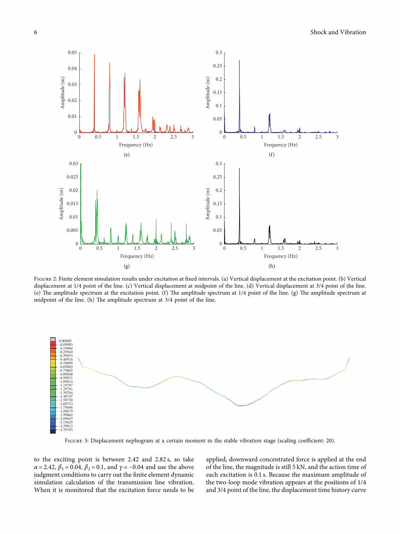
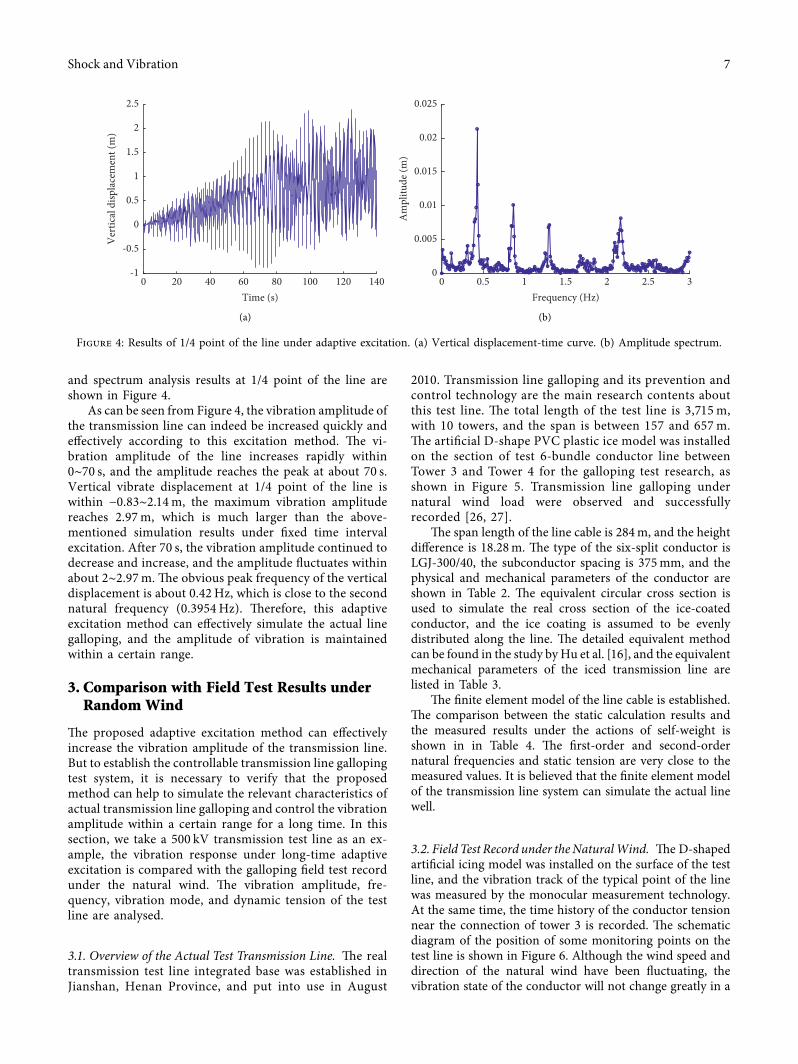
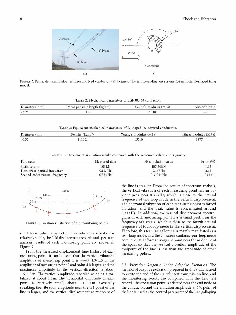