Michigan Technological UniversityDigital Commons @ Michigan

TechDissertations, Master's Theses and Master's Reports- Open Dissertations, Master's Theses and Master's Reports

2013

STUDY OF SPARK IGNITION ENGINECOMBUSTION MODEL FOR THEANALYSIS OF CYCLIC VARIATION ANDCOMBUSTION STABILITY AT LEANOPERATING CONDITIONSHao WuMichigan Technological University

Copyright 2013 Hao Wu

Follow this and additional works at: http://digitalcommons.mtu.edu/etds

Recommended CitationWu, Hao, "STUDY OF SPARK IGNITION ENGINE COMBUSTION MODEL FOR THE ANALYSIS OF CYCLIC VARIATIONAND COMBUSTION STABILITY AT LEAN OPERATING CONDITIONS", Master's report, Michigan Technological University,2013.http://digitalcommons.mtu.edu/etds/662

STUDY OF SPARK IGNITION ENGINE COMBUSTION MODEL FOR THE ANALYSIS OF CYCLIC VARIATION AND

COMBUSTION STABILITY AT LEAN OPERATING CONDITIONS

By

Hao Wu

A REPORT

Submitted in partial fulfillment of the requirements for the degree of

MASTER OF SCIENCE

In Mechanical Engineering

MICHIGAN TECHNOLOGICAL UNIVERSITY

2013

© 2013 Hao Wu

This report has been approved in partial fulfillment of the requirements for the Degree of MASTER OF SCIENCE in Mechanical Engineering.

Department of Mechanical Engineering-Engineering Mechanics

Report Advisor: Dr. Bo Chen

Committee Member: Dr. Jeffrey D. Naber

Committee Member: Dr. Chaoli Wang

Department Chair: Dr. William W. Predebon

iii

CONTENTS

LIST OF FIGURES ............................................................................................................ v

LIST OF TABLES ............................................................................................................. vi

ACKNOWLEDGEMENTS .............................................................................................. vii

ABSTRACT ..................................................................................................................... viii

1 INTRODUCTION AND MOTIVATION .................................................................. 1

2 LITERATURE REVIEW ........................................................................................... 4

2.1 LEAN COMBUSTION ANALYSIS ................................................................... 4

2.2 FUNDAMENTAL COMBUSTION MODEL ..................................................... 5

2.3 TWO-ZONE HEAT RELEASE MODEL ........................................................... 7

2.4 CYCLIC VARIATION IN ENGINE COMBUSTION ....................................... 8

3 MEAN-VALUE FUNDAMENTAL COMBUSTION MODEL FOR SPARK-IGNITION ENGINE ......................................................................................................... 10

3.1 MODEL DESCRIPTION ................................................................................... 10

3.1.1 TURBULENT ENTRAIMENT AND EDDY-BURN MODEL ................ 10

3.1.2 COMBUSTION VARIABLES ................................................................... 12

3.1.3 FLAME GEOMETRY ................................................................................ 16

3.1.4 TWO-ZONE THERMODYNAMIC MODEL ........................................... 19

3.2 MODEL CALIBRATION.................................................................................. 22

3.2.1 MODELING & CALIBRATION ENVIRONMENT ................................. 22

3.2.2 ENGINE AND OPERATING PARAMETERS USED IN SIMULATION 23

3.2.3 CALIBRATION OF MODEL PARAMETERS ......................................... 24

3.3 MODEL VALIDATION AND EXPERIMENTAL TEST RESULTS.............. 30

3.3.1 ENGINE TEST MATRIX .......................................................................... 30

3.3.2 VALIDATION RESULTS AND DISCUSSIONS ..................................... 31

4 STUDY CYCLIC VARIATION USING DEVELOPED COMBUSTION MODEL 38

4.1 CYCLIC VARIATION IN ENGINE COMBUSTION ..................................... 38

iv

4.2 CYCLIC VARIATION IN COMBUSTION SIMULATION ........................... 44

4.3 COMBUSTION STABILITY ANALYSIS ....................................................... 56

5 CONCLUSIONS AND FUTURE WORKS ............................................................. 61

REFERENCES ................................................................................................................. 63

APPENDIX A ................................................................................................................... 65

APPENDIX B ................................................................................................................... 67

v

LIST OF FIGURES

Figure 3.1: ......................................................................................................................... 12 Figure 3.2: ......................................................................................................................... 18 Figure 3.3: ......................................................................................................................... 21 Figure 3.4: ......................................................................................................................... 26 Figure 3.5: ......................................................................................................................... 27 Figure 3.6: ......................................................................................................................... 28 Figure 3.7: ......................................................................................................................... 29 Figure 3.8: ......................................................................................................................... 32 Figure 3.9: ......................................................................................................................... 32 Figure 3.10:. ...................................................................................................................... 34 Figure 3.11:. ...................................................................................................................... 34 Figure 3.12:. ...................................................................................................................... 36 Figure 3.13: ....................................................................................................................... 36 Figure 3.14:. ...................................................................................................................... 37 Figure 4.1: ......................................................................................................................... 39 Figure 4.2: ......................................................................................................................... 39 Figure 4.3: ......................................................................................................................... 40 Figure 4.4: ......................................................................................................................... 40 Figure 4.5:. ........................................................................................................................ 41 Figure 4.6: ......................................................................................................................... 42 Figure 4.7: ......................................................................................................................... 43 Figure 4.8: ......................................................................................................................... 44 Figure 4.9: ......................................................................................................................... 46 Figure 4.10:. ...................................................................................................................... 48 Figure 4.11:. ...................................................................................................................... 49 Figure 4.12:. ...................................................................................................................... 50 Figure 4.13:. ...................................................................................................................... 50 Figure 4.14:. ...................................................................................................................... 51 Figure 4.15:. ...................................................................................................................... 52 Figure 4.16:. ...................................................................................................................... 53 Figure 4.17:. ...................................................................................................................... 54 Figure 4.18:. ...................................................................................................................... 57 Figure 4.19:. ...................................................................................................................... 57 Figure 4.20:. ...................................................................................................................... 59 Figure 4.21:. ...................................................................................................................... 59 Figure 4.22:. ...................................................................................................................... 60 Figure 4.23:. ...................................................................................................................... 60

vi

LIST OF TABLES

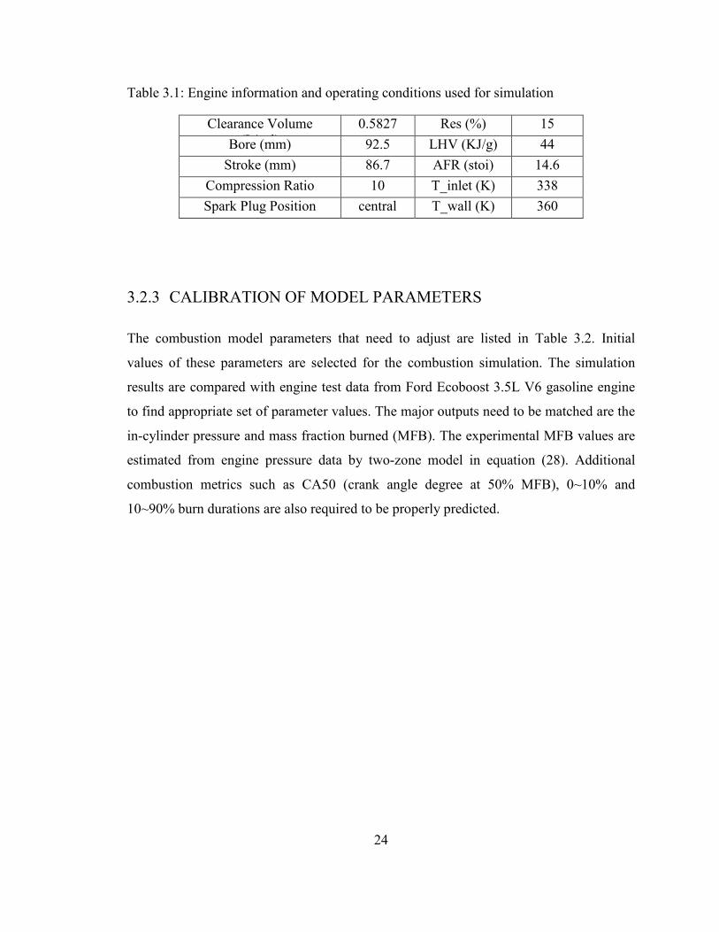
Table 3.1: Engine information and operating conditions used for simulation .................. 24

Table 3.2: Adjustable model parameters .......................................................................... 25

Table 3.3: Matrix of operation conditions of engine tests ................................................ 30

Table 3.4: Lambda sweep test conditions in simulation ................................................... 33

Table 3.5: Comparisons of CA10, CA50 and CA90 between experimental data and

simulation results .............................................................................................................. 35

Table 4.1: Amounts of introduced variation sources of engine inputs and parameters .... 45

Table 4.2: Other variation sources and their amount introduced in combustion model ... 47

Table 4.3: Variances of introduced variation sources in simulations of under different

lean conditions .................................................................................................................. 48

Table 4.4: COV of IMEP of simulation and experimental results .................................... 55

vii

ACKNOWLEDGEMENTS

Firstly I will thank my advisor Dr. Bo Chen for her advices of this report and opportunity

she provided for me to work in IC engine area. I would also thank Dr. Naber and Dr.

Wang for joining in the committee and providing me valuable opinion.

Thanks to all the lab mates in Intelligent Mechantronics and Embedded Systems Lab with

whom I have shared unforgettable time of study, work and life together. Thank all the

friends in Michigan Technological University for their help and encouragement in life

and work during these two years.

I appreciate the graduate research assistants who work in the Advance IC Engines Lab.

Their precious engine experimental data give me irreplaceable help to complete this

report.

The most people I need to thank are my parents who gave me their best and firm support

and encouragement to my study abroad. I will always remember their devotion to me and

use the effort of hard working to bring them hope in return.

viii

ABSTRACT

A fundamental combustion model for spark-ignition engine is studied in this report. The

model is implemented in SIMULINK to simulate engine outputs (mass fraction burn and

in-cylinder pressure) under various engine operation conditions. The combustion model

includes a turbulent propagation and eddy burning processes based on literature [1]. The

turbulence propagation and eddy burning processes are simulated by zero-dimensional

method and the flame is assumed as sphere. To predict pressure, temperature and other

in-cylinder variables, a two-zone thermodynamic model is used. The predicted results of

this model match well with the engine test data under various engine speeds, loads, spark

ignition timings and air fuel mass ratios. The developed model is used to study cyclic

variation and combustion stability at lean (or diluted) combustion conditions. Several

variation sources are introduced into the combustion model to simulate engine

performance observed in experimental data. The relations between combustion stability

and the introduced variation amount are analyzed at various lean combustion levels.

1

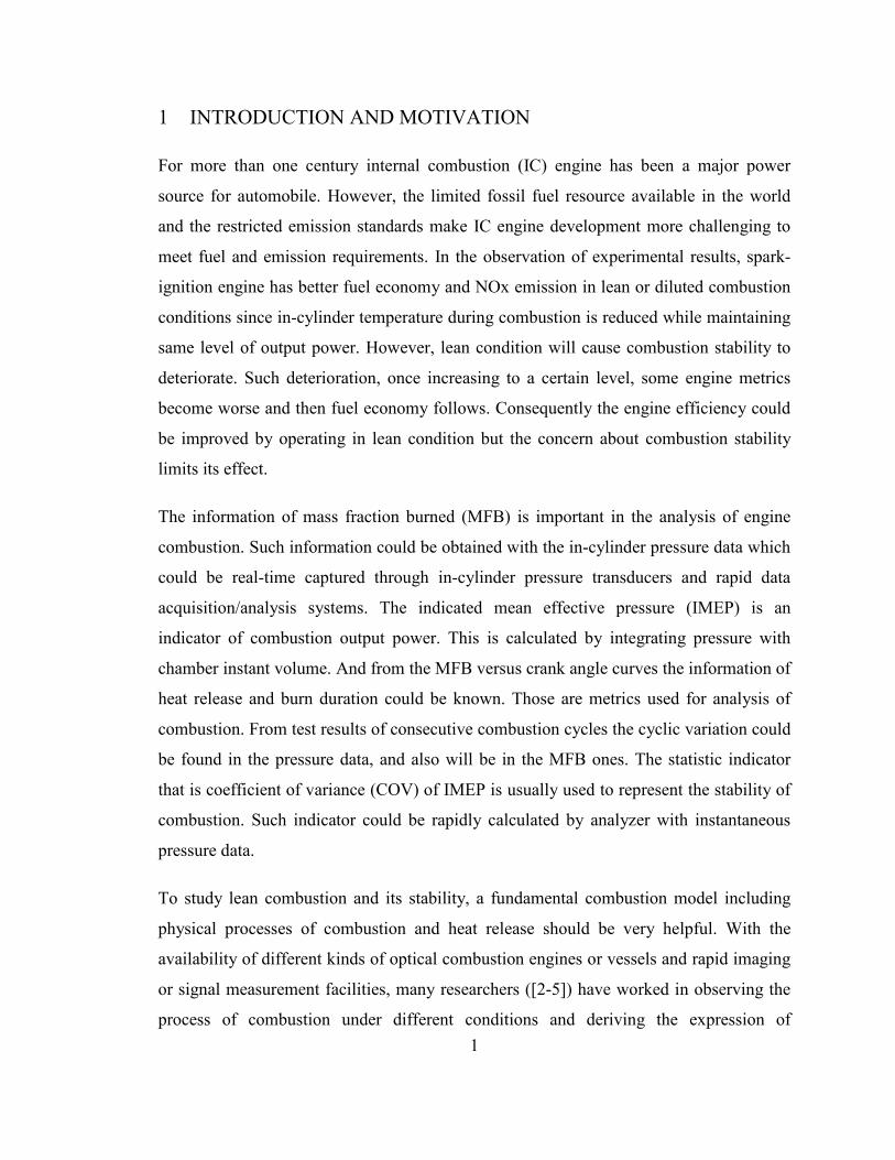
1 INTRODUCTION AND MOTIVATION

For more than one century internal combustion (IC) engine has been a major power

source for automobile. However, the limited fossil fuel resource available in the world

and the restricted emission standards make IC engine development more challenging to

meet fuel and emission requirements. In the observation of experimental results, spark-

ignition engine has better fuel economy and NOx emission in lean or diluted combustion

conditions since in-cylinder temperature during combustion is reduced while maintaining

same level of output power. However, lean condition will cause combustion stability to

deteriorate. Such deterioration, once increasing to a certain level, some engine metrics

become worse and then fuel economy follows. Consequently the engine efficiency could

be improved by operating in lean condition but the concern about combustion stability

limits its effect.

The information of mass fraction burned (MFB) is important in the analysis of engine

combustion. Such information could be obtained with the in-cylinder pressure data which

could be real-time captured through in-cylinder pressure transducers and rapid data

acquisition/analysis systems. The indicated mean effective pressure (IMEP) is an

indicator of combustion output power. This is calculated by integrating pressure with

chamber instant volume. And from the MFB versus crank angle curves the information of

heat release and burn duration could be known. Those are metrics used for analysis of

combustion. From test results of consecutive combustion cycles the cyclic variation could

be found in the pressure data, and also will be in the MFB ones. The statistic indicator

that is coefficient of variance (COV) of IMEP is usually used to represent the stability of

combustion. Such indicator could be rapidly calculated by analyzer with instantaneous

pressure data.

To study lean combustion and its stability, a fundamental combustion model including

physical processes of combustion and heat release should be very helpful. With the

availability of different kinds of optical combustion engines or vessels and rapid imaging

or signal measurement facilities, many researchers ([2-5]) have worked in observing the

process of combustion under different conditions and deriving the expression of

2

combustion variables. Base on the accessibility of such combustion variables and the

visible processes of combustion flame propagation, researchers ([1, 5-8]) have built

combustion model in spark-ignition (SI) engine including physical relations like turbulent

flame propagation and eddy burned processes to predict the fuel mass burned rate.

For the modeling of mass fraction burned curves, empirical functions like Wiebe function

are widely used with several parameters to be adjusted. Such methods could be

convenient to use to predict heat release curve for individual cycle. However,

fundamental combustion model has the advantage to apply under wide range of operation

conditions due to physical-based relations are included in the model. The heat release

information is the result of many complicated processes. Even if there is empirical

expression to model MFB information, the parameters of the expression probably have

no apparent trends or relations with the change of operation conditions. The combustion

models introduced in this report are developed to express flame structure and burning

process with the results of experimental observation. The model accuracy depends on the

chosen of parameters in both the relations of the model and the combustion

environmental conditions. The predicted results through combustion model can match the

engine tests ones perfectly with well calibrated parameters in one case. Under different

operation conditions that are considered in the model, it should still have the ability to

predict approximate results for each.

Besides the mean value trends changes along with the changing of operation condition,

the cycle-to-cycle variation in measured in-cylinder pressure histories also changes

especially under different lean or diluted levels. The variations also exist in the MFB

curves calculated from the pressure signals. Study the features of cyclic variations in the

combustion processes could be helpful and somehow necessary to understand lean

combustion and the lean limits come from instability. Such variations may be resulted by

not only the fluctuations of inputs or environment but also the random natures of flame

propagation and combustion. One advantage of fundamental combustion model is that the

random natures could be considered and simulated in the model to predicting outputs

with cyclic variations. That provides the availability to introduce variation sources with

3

reasonable variance amount in purpose of obtaining in-cylinder pressure results with

same cyclic variance level as that of experimental data.

A fundamental combustion model should have ability to predict MFB, in-cylinder

pressure values and other intermediate variables. Some of them may not be easily

observed from experiments under a wide range of operation condition. The qualified

model could help to provide physical explanations of lean combustion phenomena, to

help researchers understand how lean condition and combustion stability affect the fuel

economy. If the combustion model is good enough to precisely simulate engine

performance while changing engine inputs, it could also help to test engine strategy to see

if it fulfills the control requirements.

In this report, a historical developed fundamental combustion model is studied and

implemented. The performance of the developed combustion model is compared with

several engine test data set under different operation conditions. The presented model

includes turbulent propagation and eddy burned model introduced in [9] for mass burned

prediction. And a two-zone thermodynamic model in [10] is used for in-cylinder

pressure, mass density and temperature prediction. By introducing the randomness in

combustion variables and engine inputs, model is able to simulate the cyclic variations of

in-cylinder pressure data of consecutive cycles. The features of combustion instability of

lean combustion are studied with the simulation results from this model.

4

2 LITERATURE REVIEW

2.1 LEAN COMBUSTION ANALYSIS

Ayala et al. [11] analyze the features of lean combustion for SI engine under wide range

of operation conditions. A general phenomenon is that both engine efficiency and the

COV of IMEP increase as lambda value (lean level) increases. The COV of IMEP

increases slowly at the beginning, and after a certain lean point is reached, it raises

sharply. At the same time, the engine efficiency decreases after the lambda point where

combustion stability becomes to deteriorate. In paper [11], combustion metrics such as

burned durations are analyzed based on engine experimental results over wide range of

operation conditions. The authors found that the peak engine efficiency corresponding to

about 30 deg of 10~90% burn duration in all test. The tests also show that 2% COV of

IMEP, which is often used as the stability threshold, is corresponding to about 40 deg of

0~10% burn duration. The effect of cyclic combustion variability is also studied since it

is closely related to the efficiency change with lambda. Base on the analysis of burn

duration and IMEP of lean combustion with fixed average load, following features are

found. (1) The distribution of 10~90% burn duration is close to a normal distribution

when the lean level is low and the cyclic variation increases as lean level increases while

the distribution becomes asymmetric. (2) The distributions of 0~10% burn duration keep

normal distribution even though the combustion becomes more unstable. However the

average value of 0~10% changes significantly as lean level increases. (3) The skew like

distribution of 10~90% burn duration also appears in the distribution of IMEP. There are

small amount of cycles with extremely small IMEP values which correspond to large

10~90% burn duration. These cycles are bad combustion cycles (partial burned or

misfire) which reduce the efficiency of engine.

Ayala et al. [1] continues to study the feature of lean combustion with engine test data

and the fundamental combustion model they implemented. For the case of three

individual tests if two of them have same bias in opposite directions at the beginning of

the combustion, their deviations to the third one become large and unequal at the end of

combustion. This is why 10~90% burn duration varies significantly at very lean

5

condition. They also conclude that the cycle-to-cycle variability of combustion has close

relation with the early growth of flame. This is also found from the distribution of 0~10%

burn durations since their average values under different lean conditions change

significantly. The major cause of the slow mass burning at the early stage of combustion

is found due to the long eddy burning time under lean combustion with the help of

developed combustion model.

2.2 FUNDAMENTAL COMBUSTION MODEL

The combustion model implemented in this report includes turbulent flame propagation

and eddy burning process. Heywood introduces the turbulence flow with three

characteristic scale lengths in IC engine combustion chamber in his book [12]. The

integral macro scale ( L ) is the largest scale and reflects the size of turbulent eddies. Its

length is affected by the system boundary such as the piston height for IC engine

environment. The Kolmogorov scale ( Kl ) is the smallest scale and reflects the size of the

vortex tube. In presented model, the burning time of such small length is assumed to be

instantaneous. The third scale is Taylor microscale ( mλ ) which is the universe size of

small cells inside the integral eddies. This scale is important to the combustion model

since its size reflects the turbulent condition and affects the eddy burning time. The

length of microscale has been defined as a function of integral scale and Reynolds

number.

Blizard and Keck [6] developed the original turbulent entrainment model. The flame

propagation speed eu is assumed slowly varying and the mass burned rate is derived with

assumption of exponential eddy burning time, as shown in equations (1) and (2). The

flame geometry is assumed as spherical surface. The flame area and volume are

expressed as integrals of circle length and area of transversal surface with chamber

height. The expression of mass burned fraction is finally obtained by solving first order

6

differential equations including (1), (2), flame geometry expressions and a

thermodynamic model.

f u f em A uρ= (1)

( )( )' /

01 '

t t tb u f e f bm e A u dt m mτ ρ τ− −= − = −∫ (2)

Tabaczynski, et al. [7] modify their previous combustion model. The mass entrainment

speed ( eu ) is proportionally related to the turbulent intensity which is derived as a

function of unburned mass density ( uρ ) during the combustion. Then the eddy

entrainment speed is expressed as function of mass density as shown in equation (3).

They also give a detail solution to calculate the eddy burning time ( bτ ) according to the

single eddy burning process.

1/3

,,

ue e r

u r

u u ρρ

=

(3)

In [8], they refine their model by adding laminar flame speed term in the flame

entrainment speed ( LS ) in equation (4). They also modify the eddy burning time as the

microscale length divided by laminar flame speed shown as equation (5). That is because

the expression they solved in the previous work does not work well to express the eddy

burning time during the procedure of flame development and the flame propagation

might be in developing state for most of the combustion. The predicted MFB results from

the refined model match well with experimental data under different conditions of EGR,

lambda and spark time.

( )'e u f Lm A u Sρ= + (4)

7

LSλτ = (5)

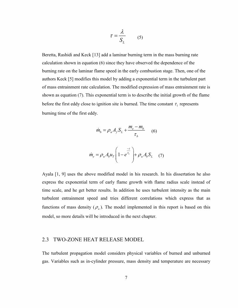
Beretta, Rashidi and Keck [13] add a laminar burning term in the mass burning rate

calculation shown in equation (6) since they have observed the dependence of the

burning rate on the laminar flame speed in the early combustion stage. Then, one of the

authors Keck [5] modifies this model by adding a exponential term in the turbulent part

of mass entrainment rate calculation. The modified expression of mass entrainment rate is

shown as equation (7). This exponential term is to describe the initial growth of the flame

before the first eddy close to ignition site is burned. The time constant 1τ represents

burning time of the first eddy.

e bb u f L

b

m mm A Sρτ−

= + (6)

11t

e u b T u b Lm A u e A Sτρ ρ−

= − +

(7)

Ayala [1, 9] uses the above modified model in his research. In his dissertation he also

express the exponential term of early flame growth with flame radius scale instead of

time scale, and he get better results. In addition he uses turbulent intensity as the main

turbulent entrainment speed and tries different correlations which express that as

functions of mass density ( uρ ). The model implemented in this report is based on this

model, so more details will be introduced in the next chapter.

2.3 TWO-ZONE HEAT RELEASE MODEL

The turbulent propagation model considers physical variables of burned and unburned

gas. Variables such as in-cylinder pressure, mass density and temperature are necessary

8

to solve the equations and to calculate other combustion variables such as turbulent

intensity and laminar flame speed.

Guezennec, et al. [10] use the two-zone (burned and unburned zones) model to predict

variables during combustion with in-cylinder pressure data. The model covers the process

from the intake valves closing to exhaust valves opening. Both of the burned and

unburned zones have their individual temperature, mass and volume, but the pressure is

same all around the chamber. The heat transfer to the chamber wall or piston is

considered and it is assumed no heat transfer between two zones. As a result this two-

zone model predicts more reasonable mass fraction burned values and it makes more

variables are available to be accessed. Yeliana, et al. [14] compares the performance of

single-zone and two-zone heat release models in an ethanol and gasoline blended fuel

engine. Both heat transfer and crevice volume factors are considered in the models.

2.4 CYCLIC VARIATION IN ENGINE COMBUSTION

Cycle-to-cycle variation exits in the combustion process as presented in real engine tests.

This variation is more severe under lean or diluted conditions.

Rashidi [15] studies the cycle-to-cycle variation with photographs taken from a

transparent piston engine. A period from the spark occurrence to a formed stabilized

flame kernel is observed and defined as ignition delay. From the observation, the

variations of both the length of the period and the time of its formation exist among

consecutive combustion cycles. The shapes of flame fronts right after the stabilized

flames are different due to the variation of the flow velocities. It is also concluded that

the length of this flame stabilization period could be influenced by the turbulent structure,

and it is also the major cause of cyclic variation of the combustion process. The variation

of the main part of the flame propagation is also affected by the turbulent velocity and

structure.

9

Keck et al. [5] study the early flame development process with an optical combustion

chamber piston engine. From the observation of several combustion tests, it is found that

the real flame kernels have random locations around the spark plug and their distribution

has different trends under different mixtures of flow conditions. The authors conclude

that the randomness of the early flame kernel is one of the major causes of the cyclic

combustion variation. Also, the variations of burning speed and the first eddy size after

ignition play the essential roles to the fluctuation of early stage combustion. The initial

burning speed is mainly laminar flame speed and it is affected by the mixture situation

near the spark site. The variation of first eddy size is caused by the fluctuation of

turbulent structure of each cycle.

Aghdam et al. [16] summarize several cyclic variation sources and include the fluctuation

of turbulent flow into their combustion model. The cyclic variations of engine

combustion could be easily observed from in-cylinder pressure, combustion phasing and

combustion duration. However, the origins of cyclic variations may come from (1) the

turbulent intensity, (2) engine inputs (lambda, air flow, et al), (3) the mixture composition

near the spark plug and (4) the spark ignition process. The authors observe the peak

pressure versus peak pressure location (crank angle) scatters and their distributions

comparing with those from engine data. By adjusting the variation level of the turbulent

fluctuations, the model could simulate engine outputs with similar variations to those of

experimental data.

10

3 MEAN-VALUE FUNDAMENTAL COMBUSTION MODEL FOR SPARK-IGNITION ENGINE

In this chapter, a fundamental combustion model is implemented combining with two-

zone thermodynamic model. The predicted results of the model are compared with engine

test data recorded by ACAP data acquisition system developed by the DSP Technology

Inc. It is used for a Ford Ecoboost 3.5L V6 DI gasoline engine. The performance of the

model is tuned by changing some model parameters and unmeasured engine inputs.

3.1 MODEL DESCRIPTION

The fundamental combustion model presented in this report is a turbulent propagation

and eddy burning model to predict the mass burned rate. Unlike some of the early works

that are achieved by solving differential equations, the presented model is achieved by

writing in discrete form with basic Euler integral method. No iterations are needed to

improve the solution. Besides, the variables of unburned gas are predicted with two-zone

thermodynamic model and the geometry of flame is assumed spherical with growing

radius.

3.1.1 TURBULENT ENTRAIMENT AND EDDY-BURN MODEL

The turbulent entrainment model described in [9] is employed. The turbulent flame

entrains the unburned gas from a spherical surface with the rate related to the laminar

flame speed and turbulent intensity. Unburned gas in or out of flame has turbulent

structure, so it can be described with the three characteristic lengths. The unburned gas

entrained into the flame will be burned with laminar flame speed in the unit of microscale

length ( mλ ). Equations (8) to (10) are the expressions of the combustion model.

1' 1t

eu e L

dm A S u edt

τρ−

= + − (8)

11

b e bu e L

b

dm m mA Sdt

ρτ−

= + (9)

mb

LSλτ = (10)

Equation (8) is the expression of entrainment mass ( em ) rate which contains a laminar

burning component ( LS ) and a turbulent propagation one ( 'u ). The unburned mass

density ( uρ ) multiplies by the entrained flame front area ( eA ) represents the entrained

volume of each step. The turbulent propagation component is multiplied by an

exponential term to describe the development of early flame growth of the combustion

cycle. The value of the exponential term increases from zero to full turbulent intensity.

With a time constant ( 1τ ) defined as burning time of the first eddy after ignition. As

shown in Figure 3.1, the turbulent intensity reaches around 2/3 of full scale at time equal

to the time constant bτ =10. The shorter the time constant is, the quicker the turbulent

propagation dynamics is. In the presented model, the time constant is chosen one fifth of

the original value which results in much quicker exponential term. The value of this time

constant affects the flame propagation speed significantly. However, the definition of this

parameter is not firmly defined in previous research. So, it will be a tunable parameter for

the presented model. The selection of this parameter’s value will be discussed in the

model calibration section.

12

Figure 3.1: Growing of exponential term with time constant of 10ms

Equation (9) describes the calculation of burned mass ( bm ) rate. The first component is

the laminar mass burning occurred in front of the flame surface. The second component,

which is the major part, represents the burning of unburned gas entrained by the flame.

The denominator is the characteristic time ( bτ ), the eddy burning time expressed by

equation (10). The definition of the eddy burning time is the time to burn up a single cell

of Taylor microscale length ( mλ ) with laminar flame speed ( LS ). The ratio of the

entrained unburned mass ( e bm m− ) to the eddy burning time is the component of mass

burned rate inside the entrained gas fuel mixture.

3.1.2 COMBUSTION VARIABLES

From the description of combustion model, it is clear that the mass burning rate is

estimated by modeling the turbulent movement and eddy burning process. To accomplish

this model the correlations of the variables including laminar flame speed, turbulent

intensity and turbulent microscale length need to be known. The values of these variables

changes as the environmental condition changes. Their relations have been derived and

summarized from experimental observation of combustion by many researches. In this

section the correlations of these variables used in the presented model are introduced.

13

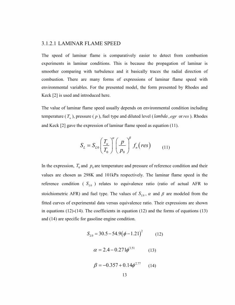
3.1.2.1 LAMINAR FLAME SPEED

The speed of laminar flame is comparatively easier to detect from combustion

experiments in laminar conditions. This is because the propagation of laminar is

smoother comparing with turbulence and it basically traces the radial direction of

combustion. There are many forms of expressions of laminar flame speed with

environmental variables. For the presented model, the form presented by Rhodes and

Keck [2] is used and introduced here.

The value of laminar flame speed usually depends on environmental condition including

temperature ( uT ), pressure ( p ), fuel type and diluted level ( lambda , egr or res ). Rhodes

and Keck [2] gave the expression of laminar flame speed as equation (11).

( )00 0

uL L n

T pS S f resT p

α β

=

(11)

In the expression, 0T and 0p are temperature and pressure of reference condition and their

values are chosen as 298K and 101kPa respectively. The laminar flame speed in the

reference condition ( 0LS ) relates to equivalence ratio (ratio of actual AFR to

stoichiometric AFR) and fuel type. The values of 0LS , α and β are modeled from the

fitted curves of experimental data versus equivalence ratio. Their expressions are shown

in equations (12)-(14). The coefficients in equation (12) and the forms of equations (13)

and (14) are specific for gasoline engine condition.

( )20 30.5 54.9 1.21LS φ= − − (12)

3.512.4 0.271α φ= − (13)

2.770.357 0.14β φ= − + (14)

14

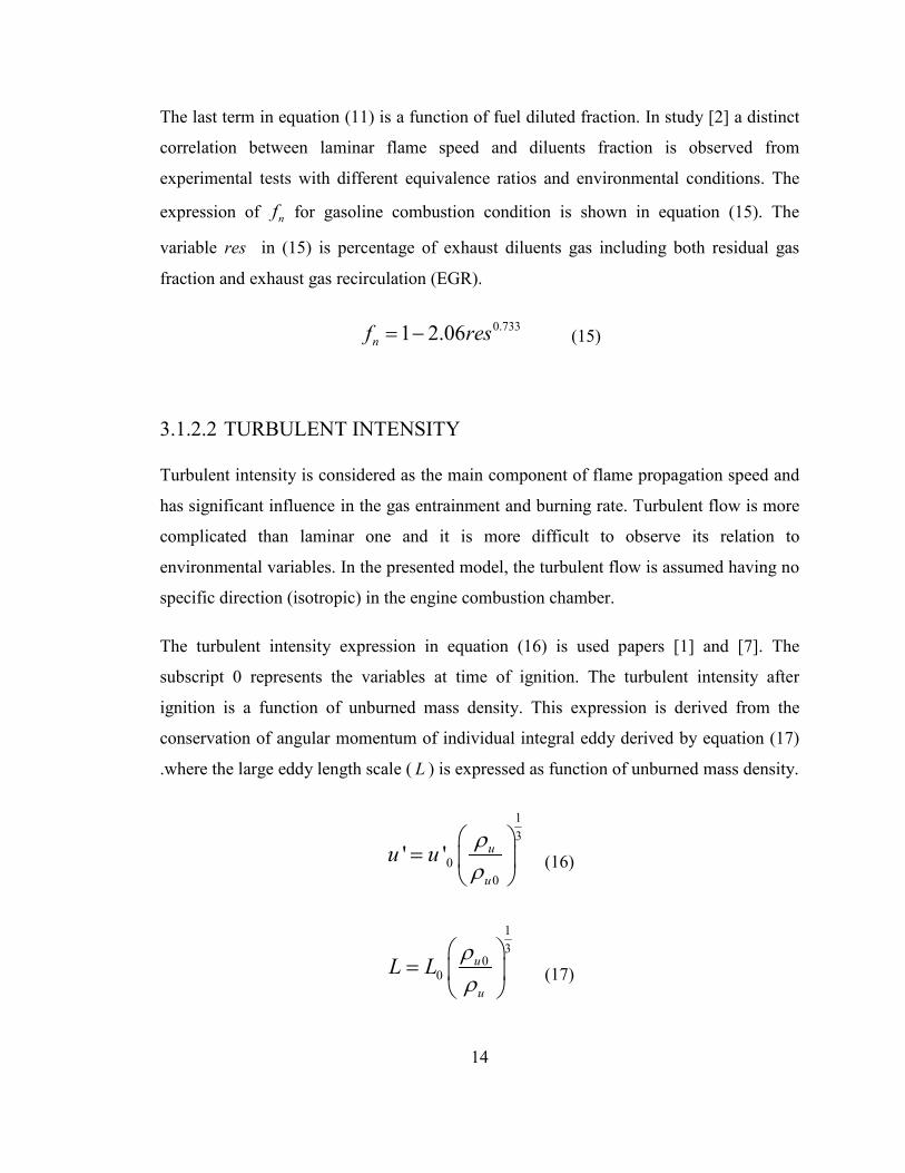
The last term in equation (11) is a function of fuel diluted fraction. In study [2] a distinct

correlation between laminar flame speed and diluents fraction is observed from

experimental tests with different equivalence ratios and environmental conditions. The

expression of nf for gasoline combustion condition is shown in equation (15). The

variable res in (15) is percentage of exhaust diluents gas including both residual gas

fraction and exhaust gas recirculation (EGR).

0.7331 2.06nf res= − (15)

3.1.2.2 TURBULENT INTENSITY

Turbulent intensity is considered as the main component of flame propagation speed and

has significant influence in the gas entrainment and burning rate. Turbulent flow is more

complicated than laminar one and it is more difficult to observe its relation to

environmental variables. In the presented model, the turbulent flow is assumed having no

specific direction (isotropic) in the engine combustion chamber.

The turbulent intensity expression in equation (16) is used papers [1] and [7]. The

subscript 0 represents the variables at time of ignition. The turbulent intensity after

ignition is a function of unburned mass density. This expression is derived from the

conservation of angular momentum of individual integral eddy derived by equation (17)

.where the large eddy length scale ( L ) is expressed as function of unburned mass density.

13

00

' ' u

u

u u ρρ

=

(16)

13

00

u

u

L L ρρ

=

(17)

15

The initial turbulent intensity 0'u was assumed to be proportional to the mean piston

speed in the model introduced in [8]. However, Keck [3] summarized the relation of

initial turbulent intensity expressed as equation (18) with groups of experimental data. In

equation (18) the initial turbulent intensity is a function of the mean piston speed ( pu )

and the ratio of unburned mass density to the mass density of inlet gas (mass density after

intake valve closing). After implementing this equation into the presented model, it is

found that the root square term in equation (18) may not be appropriate comparing with

Ecoboost data. To provide the flexibility of the developed model, the parameter C and

the order of the density ratio are adjustable for the model calibration.

12

00' u

p

in

u C u ρρ

= ⋅ ⋅

(18)

3.1.2.3 TURBULENCE MICROSCALE LENGTH

The turbulence microscale length also called Taylor microscale length ( mλ ) illustrates the

size of dissipative cells in turbulent eddies. In the combustion model, the value of

microscale length is necessary for the calculation of eddy burning time in equation (10).

Tennekes [17] gives the definition of the ratio of Taylor microscale length to turbulent

integral length ( L ) as a function of Reynolds number ( tRe ) in equation (19).

0.5RemtC

Lλ −= ⋅ (19)

'Re ut

u Lρµ

= (20)

Equation (20) is the definition of Reynolds number for gas flow in the engine combustion

chamber. The velocity of flow is represented by turbulent intensity 'u and the

characteristic dimension is represented by turbulence integral length ( L ). The dynamic

16

viscosity of flow ( µ ) is related to environmental temperature. Substituting the

expressions of turbulent intensity after ignition in equations (16) and (17) and assuming

that the integral length is proportional to the chamber height ( )h θ , the microscale length

could be expressed as equation (21). The subscript 0 represents the parameter values at

spark ignition. Constant 'C is an adjustable parameter for model calibration.

12

0.5

1 512 6

' 0 30

0

Re'

1'

m tu

uu

LC L Cu

hCu

µλρ

µ ρρ

− = ⋅ ⋅ = ⋅

⋅= ⋅

(21)

3.1.3 FLAME GEOMETRY

In the presented model, the flame front is assumed spherical surface based on the

conclusions of several experimental observations without swirl ([3], chapter 9 of [12]).

Many researchers (discussed in literature review) have built their combustion models

with such assumption. The ignition locates in the center of cylinder head for Ford

Ecoboost gasoline engine. For the purpose of simplified calculation the electrodes of

spark plug are assumed just in the plane of the cylinder head in the model. The radius of

the flame propagates with the same speed as gas entrainment speed: laminar burning

speed and turbulent intensity with exponential development factor at early stage. The

flame entrained area and volume will be calculated with semi-spherical surface and

volume equations (22) and (23).

22 rA spheresemi π=− (22)

17

3

32 rV spheresemi π=− (23)

For the condition in engine combustion chambers, since combustion starts close to the top

dead center (TDC), the flame front will reach the piston head firstly and then chamber

wall while propagating. The process of flame geometry development is shown in Figure

3.2. Figure 3.2 (a) is the early stage of flame formation and the flame is half of sphere.

From the observation of early flame formation in [5] the shape of flame at that stage

covers around the spark plug and is equivalent to sphere. Due to the small area or volume

of the flame at this stage, is does not induce much changes of in-cylinder pressure and

heat release. Soon after the ignition the flame will reach piston head as shown in Figure

3.2 (b) and it will mainly propagate along with the radial direction until reaching the

chamber wall shown in Figure 3.2 (c). During (b) and (c) stages, the flame shapes are

partial semi-spheres and the calculations of their surface areas and volumes are shown in

equations (24) and (25). For the condition of (c) the flame is not only “cut” from bottom

but also side. At the end of propagation, the flame fully fills the combustion chamber as

shown in Figure 3.2 (d). The flame front area becomes zero and the volume becomes the

maximum. Usually, the energy released from combustion increases the most quickly

during this period.

18

(a)

(b)

(c)

(d)

Figure 3.2: Flame geometry propagation process in engine combustion chamber, (a) the early state, (b) flame front reaches piston head, (c) flame front reaches cylinder wall, (d)

flame and burned gas fully fill the combustion chamber.

rhA spherepartial π2=− (24)

32

31 hhrV spherepartial ππ −=− (25)

The intersection between flame and chamber wall is considered not only for the flame

geometry aspect but also for the contact area between flame and chamber wall (including

cylinder head and piston). The amount of energy from heat transfer to chamber wall or

19

piston is closely related to the contact area, the detail will be discussed in the next

section. The method to calculate contact area is apparent after determining the geometry

of combustion flame. It is needed to mention that when the flame fully fills the chamber

in stage (d), the contact area will be the inner surface area of the combustion chamber.

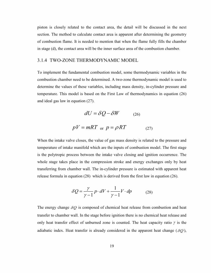
3.1.4 TWO-ZONE THERMODYNAMIC MODEL

To implement the fundamental combustion model, some thermodynamic variables in the

combustion chamber need to be determined. A two-zone thermodynamic model is used to

determine the values of these variables, including mass density, in-cylinder pressure and

temperature. This model is based on the First Law of thermodynamics in equation (26)

and ideal gas law in equation (27).

dU Q Wδ δ= − (26)

pV mRT= or p RTρ= (27)

When the intake valve closes, the value of gas mass density is related to the pressure and

temperature of intake manifold which are the inputs of combustion model. The first stage

is the polytropic process between the intake valve closing and ignition occurrence. The

whole stage takes place in the compression stroke and energy exchanges only by heat

transferring from chamber wall. The in-cylinder pressure is estimated with apparent heat

release formula in equation (28) which is derived from the first law in equation (26).

11 1

Q p dV V dpγδγ γ

= ⋅ + ⋅− − (28)

The energy change Qδ is composed of chemical heat release from combustion and heat

transfer to chamber wall. In the stage before ignition there is no chemical heat release and

only heat transfer effect of unburned zone is counted. The heat capacity ratio γ is the

adiabatic index. Heat transfer is already considered in the apparent heat change ( Qδ ),

20

otherwise the heat capacity ration ( γ ) value in equation (28) could be replaced by

polytropic coefficient which is usually smaller.

The estimation of heat transfer amount of each crank angle step is expressed in equation

(29) according paper [5]. The direction of heat transfer calculated by equation (29) is

from unburned gas to chamber wall. Since this model is crank angle-based, engine speed

( N ) needs to be considered to convert from time-based equation. The heat transfer

constant hth could be determined from Woschni’s work [18] in equation (30).

( ) /ht contact ht walldQ A h T T N= − (29)

0.2 0.8 0.8 0.53ht hth C d p w T− −= ⋅ ⋅ ⋅ ⋅ (30)

In equation (30), d is the characteristic length and it is engine cylinder bore length here,

p and T are in-cylinder pressure and temperature respectively, w is the characteristic

speed and the mean piston speed is used. The constant htC is an adjustable parameter for

model calibration. Woschni gave a value of 110 for parameter htC as recommendation.

However, due to the different usage of hth (divided by engine speed in the present

model), its value should be in various scales. The detail of tuning this parameter will be

discussed in the model calibration section.

The second stage starts from ignition and ends with the opening of exhaust value. The

second stage ends when all chemical energy releases out. Without more chemical heat

release, it returns to polytropic process in the cylinder like the first stage. The model of

this stage is considered two-zone: burned and unburned zone as shown in Figure 3.3. The

two-zone model follows the first law of thermodynamics and the fuel loss in crevice is

not considered.

21

Figure 3.3: Schematic diagram of two-zone combustion thermodynamic model.

The two zones have differences in all states except with the same pressure during all

time. The value of unburned mass density is necessary for the estimation of flame

propagation and mass burned rate in equations (8) and (9). Pressure and temperature in

unburned area are also needed for the estimation of other variables in combustion.

Temperature in burned area could be used to approximate determine the heat capacity

information ( pc vc γ ). Equation (31) is the expression of energy distribution of two-zone

model based on first law of thermodynamics in equation (26).

( )

( ) ( ), , /

b LHV cb vb b u vu u b vb b vu u

u ht u u wall b ht b b wall

m Qm c dT m c dT m c T c TAFR

A h T T A h T T N pdV

δ ηδ ⋅+ + − =

− − + − − (31)

b and u in the subscripts represent variables in burned and unburned zones, respectively.

The left side of equation (31) is the internal energy change of one discrete step for the

whole chamber. The third term represents the internal energy change of the burned mass

in current step. In the right side, the first term is the chemistry energy released from the

fuel with a combustion efficiency term ( cη ). All the mass variables in the model are mass

of gas mixture without fuel because it is hard to trace the mass density with direct

injection (DI) fuel delivery method as Ecoboost has, and the injection time and

vaporization percentage are not considered. That is the reason that only air fuel ratio

22

(AFR) is listed in the denominator of first term in the right. Second term is the heat

transfer amount of both zones and the expression has been discussed previously.

The mass densities of both zones are hard to estimate during the early combustion. The

mass and volume of burned gas are small so the part between burned gas and flame front

could not be neglected. To find approximate value of unburned mass density, equation

(32) which is derived from features of adiabatic process is used. Temperature of

unburned zone can be calculated accordingly with ideal gas law in equation (27). Then

only one variable which is the temperature of burned zone is unknown in equation (31).

2 2

1 1

pp

γρρ

=

(32)

The volume of burned zone is assumed the same as the spherical flame volume with the

calculation method described in previous section. One limitation is that the area between

the burned and unburned zones (entrained in flame and not burned) is not considered. As

studied by Keck [3], there is small difference between the burned surface and the flame

surface which depends on the turbulent microscale length. In the presented model, they

are assumed the same for simplification since there is no rigid accuracy requirement in

the estimation of the geometries of two zones.

3.2 MODEL CALIBRATION

The parameters of combustion model need to be adjusted to predict proper output values

that fit to experimental results under specific engine combustion condition. Increase the

number of adjustable parameters increases the degree of freedom and also the difficulty

of the model tuning.

3.2.1 MODELING & CALIBRATION ENVIRONMENT

23

The presented combustion model is written in SIMULINK graphical programming

environment for ease of modification and calibration. The MATLAB/SIMULINK has

strong computational power and user friendly interface for parameterization and

programming. The inputs of engine operation and the parameters of engine model are

defined in an initial MATLAB .m file. The experimental data acquired by ACAP system

are logged and loaded as .mat data file into MATLAB workspace. These experimental

data are used as a base for the calibration of model parameters. The combustion .mdl file

in SIMULINK can be integrated with other sub-systems of vehicle or control strategies

for engine or vehicle tests.

3.2.2 ENGINE AND OPERATING PARAMETERS USED IN

SIMULATION

Table 3.1 lists the engine information and operating conditions used for simulation. The

left column contains the engine specific information and the right column gives the

values of operating variables. The “Res (%)” represents the percentage of residual gas

fraction. The residual gas is the gases that remain in the cylinder after the exhaust stroke

has been completed and the recirculated gas from intake pipe during the overlap between

intake valve opening and exhaust valve closing. Unlike EGR value, the residual gas

fraction cannot be measured from oxygen sensors mounted on intake and exhaust pipes.

Fox [19] gives the estimation method for the residual gas fraction of a gasoline engine.

However, some of parameters for the estimation are not available yet. The value of 15%

is assumed in the simulation. The values of lower heating value (LHV) and AFR at

stoichiometric condition are selected as those values provided in the appendix of

Heywood’s book [12]. The temperature of chamber wall is chosen based on the average

values of engine dyno test data. The temperature of inlet gas (T_inlet) influences the total

mass amount taken into the combustion. Its value is presumed based on the in-cylinder

pressure matching with experimental results.

24

Table 3.1: Engine information and operating conditions used for simulation

Clearance Volume (L/ l)

0.5827 Res (%) 15 Bore (mm) 92.5 LHV (KJ/g) 44

Stroke (mm) 86.7 AFR (stoi) 14.6 Compression Ratio 10 T_inlet (K) 338 Spark Plug Position central T_wall (K) 360

3.2.3 CALIBRATION OF MODEL PARAMETERS

The combustion model parameters that need to adjust are listed in Table 3.2. Initial

values of these parameters are selected for the combustion simulation. The simulation

results are compared with engine test data from Ford Ecoboost 3.5L V6 gasoline engine

to find appropriate set of parameter values. The major outputs need to be matched are the

in-cylinder pressure and mass fraction burned (MFB). The experimental MFB values are

estimated from engine pressure data by two-zone model in equation (28). Additional

combustion metrics such as CA50 (crank angle degree at 50% MFB), 0~10% and

10~90% burn durations are also required to be properly predicted.

25

Table 3.2: Adjustable model parameters

Parameters Expression/Description

1const '

0 1'uind

up

in

u const u ρρ

= ⋅ ⋅

'uind

2const ( )1 5

12 63

2 00

1'm u

u

h SIconst

uµ

λ ρρ

⋅ = ⋅

nτ /' 1 b

tne

u e Ldm A S u edt

ττρ−

= + −

htC 0.80.2 0.8 0.53

pht hth C B p u T− −= ⋅ ⋅ ⋅ ⋅

cγ eγ Heat capacity ratios of compression and

expansion strokes

cη Combustion efficiency

CALIBRATION OF PARAMETERS: 1const AND 2const

The MFB values are sensitive to the turbulent intensity and microscale length. The

related parameters could be calibrated based on how well the simulation results match to

the engine test results. Parameters 1const and 2const are the most direct factors to

influence the turbulent intensity and microscale length. The secondary important

parameters, 'uind is initially chosen to be 1/3 as recommended in [3] and nλ is chosen to

be 5 as discussed earlier.

The predicted curves of entrained mass and burned mass versus crank angle during

combustion for one test are shown in Figure 3.4. The entrainment process ends when the

26

flame fully fills the combustion chamber. At this moment some of mixture entrained in

flame is still burning with laminar flame speed. So the burned mass reaches the final

value later than the entrained mass.

Figure 3.4: Entrained and burned mass history during combustion by simulation, 2000 rpm, 5 bar BMEP, lambda = 1, MBT

The parameter 1const influences the phase of the entrained mass curve since the

turbulent intensity is the major impact factor of the mass entrainment speed. Large

turbulent intensity leads early completion of mass entrainment and indirectly advances

mass burning curve. The parameter 2const relates to the microscale length and the eddy

burning time. Large microscale length results in long eddy burning time and the entrained

mass will burn slowly. Usually, the mass burning has the maximum rate when the

entrainment ends. This can be seen from the equation (9) since the largest difference

between the entrained mass and burned mass occurs at the end of entrainment. So, the

crank angle at end of entrainment could be or close to the maximum heat release rate

27

point. Figure 3.5 (a) compares the simulated heat release rate during combustion with the

experimental heat release rate curve which is estimated from pressure data. Figure 3.5 (b)

compares the simulated het release with experimental result. The heat release values are

the mean values of 300 consecutive combustion cycles.

(a) (b)

Figure 3.5: Predicted and experimental heat release rate and hear release data, 2000 rpm, 5 bar BMEP, lambda = 1, MBT.

The simulated maximum heat release rate point is advanced comparing with that of

experimental data. This may be caused by a sudden end of mass entrainment in the

simulation. In addition, unable to simulate the trend of mass burning rate correctly after

the entrainment ends could be another reason to cause this mismatch. The simulated heat

release curve is close to the experimental result as shown in Figure 3.5 (b).

CALIBRATION OF GAMMA, htC AND cη

To appropriately predict heat release, the acceptable in-cylinder pressure data are needed.

If the heat release information is successfully simulated but there is an apparent

difference between the simulated in-cylinder pressures and experimental data, it means

28

that some parameters related to total released energy are not well chosen. The parameters

related to total released energy include combustion efficiency ( cη ), heat transfer ( htC

wallT ), inlet gas temperature ( inT ) and heat capacity ratio ( cγ eγ ).

The combustion efficiency can be referred from figure 3-9 of Heywood’s book [12] as a

function of equivalence ratio for gasoline engine. The heat capacity ratio (gamma) of

adiabatic process generally depends on the temperature and composition of gas mixture.

The gamma value in compression stroke can be adjusted by the pressure curve before

spark ignition. In expansion stroke, the value is lower due to high temperature and more

product of combustion in the mixture. The amount of heat transfer can be referred from

some universal energy distributions for general gasoline engines, for example, on page 27

of [20]. The temperature of inlet gas is a direct parameter to predict the overall amount of

gas mass for each cycle. All these parameters need to be chosen to make in-cylinder

pressure values close to experimental data while predicting reasonable intermediate

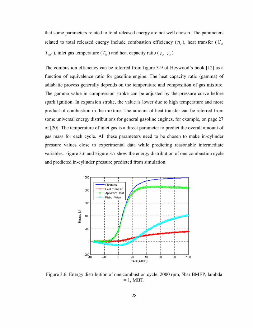
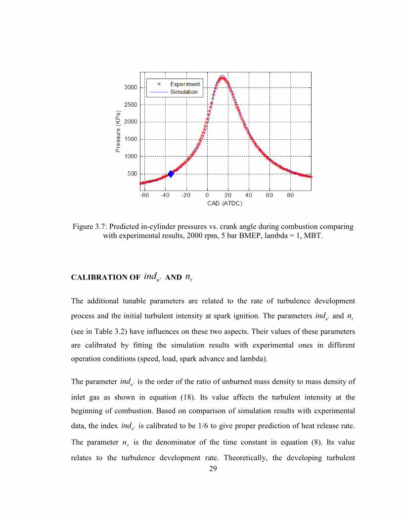
variables. Figure 3.6 and Figure 3.7 show the energy distribution of one combustion cycle

and predicted in-cylinder pressure predicted from simulation.

Figure 3.6: Energy distribution of one combustion cycle, 2000 rpm, 5bar BMEP, lambda = 1, MBT.

29

Figure 3.7: Predicted in-cylinder pressures vs. crank angle during combustion comparing with experimental results, 2000 rpm, 5 bar BMEP, lambda = 1, MBT.

CALIBRATION OF 'uind AND nτ

The additional tunable parameters are related to the rate of turbulence development

process and the initial turbulent intensity at spark ignition. The parameters 'uind and nτ

(see in Table 3.2) have influences on these two aspects. Their values of these parameters

are calibrated by fitting the simulation results with experimental ones in different

operation conditions (speed, load, spark advance and lambda).

The parameter 'uind is the order of the ratio of unburned mass density to mass density of

inlet gas as shown in equation (18). Its value affects the turbulent intensity at the

beginning of combustion. Based on comparison of simulation results with experimental

data, the index 'uind is calibrated to be 1/6 to give proper prediction of heat release rate.

The parameter τn is the denominator of the time constant in equation (8). Its value

relates to the turbulence development rate. Theoretically, the developing turbulent

30

intensity grows fully when the first eddy completes burning. As discussed previously, the

value of τn is chosen to be 5 to speed up turbulent propagation.

3.3 MODEL VALIDATION AND EXPERIMENTAL TEST RESULTS

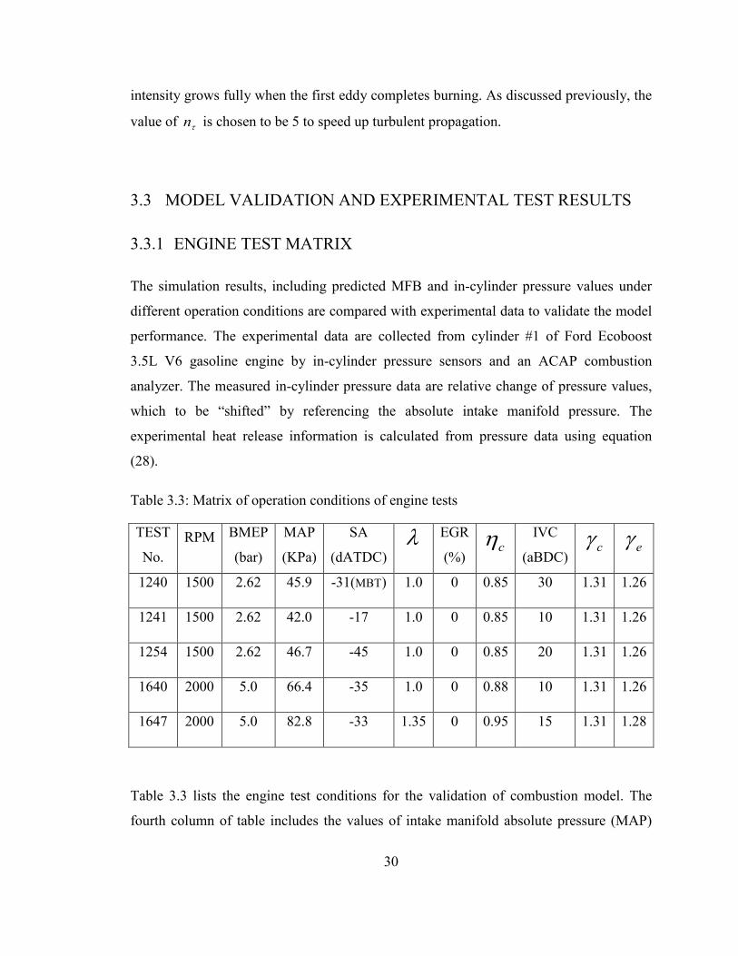
3.3.1 ENGINE TEST MATRIX

The simulation results, including predicted MFB and in-cylinder pressure values under

different operation conditions are compared with experimental data to validate the model

performance. The experimental data are collected from cylinder #1 of Ford Ecoboost

3.5L V6 gasoline engine by in-cylinder pressure sensors and an ACAP combustion

analyzer. The measured in-cylinder pressure data are relative change of pressure values,

which to be “shifted” by referencing the absolute intake manifold pressure. The

experimental heat release information is calculated from pressure data using equation

(28).

Table 3.3: Matrix of operation conditions of engine tests

TEST

No. RPM BMEP

(bar)

MAP

(KPa)

SA

(dATDC) λ

EGR

(%) cη

IVC

(aBDC) cγ eγ

1240 1500 2.62 45.9 -31(MBT) 1.0 0 0.85 30 1.31 1.26

1241 1500 2.62 42.0 -17 1.0 0 0.85 10 1.31 1.26

1254 1500 2.62 46.7 -45 1.0 0 0.85 20 1.31 1.26

1640 2000 5.0 66.4 -35 1.0 0 0.88 10 1.31 1.26

1647 2000 5.0 82.8 -33 1.35 0 0.95 15 1.31 1.28

Table 3.3 lists the engine test conditions for the validation of combustion model. The

fourth column of table includes the values of intake manifold absolute pressure (MAP)

31

which is an indication of engine load. The electronic throttle angle is chosen to maintain

the required brake mean effect pressure (BMEP) output. The spark advance (SA) is the

crank angle of spark ignition. Maximum brake torque (MBT) point is chosen by adjust

the CA50 around 7~9 deg after top dead center (ATDC). For each engine test condition,

the mean value of in-cylinder pressure data of 300 consecutive combustion cycles is used

to calculate experimental heat release and use these values to compare with simulation

results.

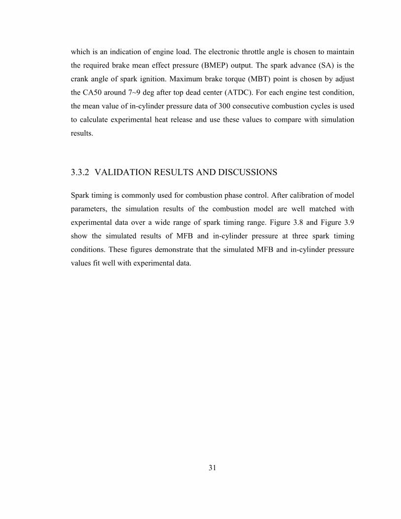
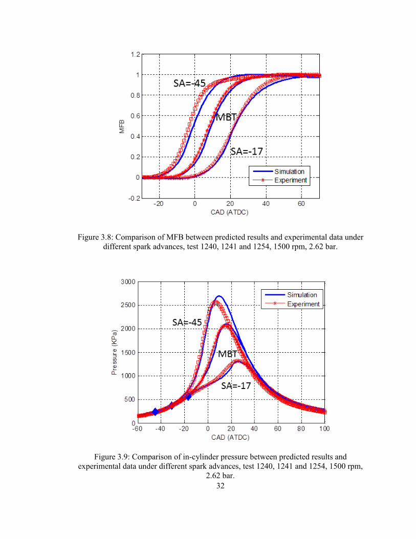
3.3.2 VALIDATION RESULTS AND DISCUSSIONS

Spark timing is commonly used for combustion phase control. After calibration of model

parameters, the simulation results of the combustion model are well matched with

experimental data over a wide range of spark timing range. Figure 3.8 and Figure 3.9

show the simulated results of MFB and in-cylinder pressure at three spark timing

conditions. These figures demonstrate that the simulated MFB and in-cylinder pressure

values fit well with experimental data.

32

Figure 3.8: Comparison of MFB between predicted results and experimental data under different spark advances, test 1240, 1241 and 1254, 1500 rpm, 2.62 bar.

Figure 3.9: Comparison of in-cylinder pressure between predicted results and experimental data under different spark advances, test 1240, 1241 and 1254, 1500 rpm,

2.62 bar.

33

To validate the performance of the combustion model at lean combustion situation, a set

of lambda sweep tests are performed. Table 3.4 lists the parameters gamma and

combustion efficiency values used in the simulation. In lambda sweep tests, the lambda

value varies from 1 to 1.35 with 0.05 as increment. The engine runs at 2000 rpm and 5

bar BMEP. The heat capacity ratio in expansion process ( eγ ) is chosen based on the in-

cylinder temperature reduction and the air composition in the mixture. The values of the

combustion efficiency cη are referred from figure 3-9 of Heywood [12] with the

consideration of matching the experimental pressure results. Figure 3.10 and Figure 3.11

show the comparison of simulated MFB and pressure with experimental results. The

simulation results match the experimental data properly with the calibrated parameter

values.

Table 3.4: Lambda sweep test conditions in simulation

TEST Lambda eγ cη

1640 1.0 1.26 0.85

1641 1.05 1.26 0.90

1642 1.1 1.26 0.90

1643 1.15 1.27 0.92

1644 1.2 1.27 0.95

1645 1.25 1.27 0.95

1646 1.3 1.28 0.95

1647 1.35 1.28 0.95

34

Figure 3.10: Comparison of MFB vs. crank angle with experimental data of test 1640 (lambda = 1.0) and 1647 (lambda = 1.35).

Figure 3.11: Comparison of in-cylinder pressure vs. crank angle with experimental data of test 1640 (lambda = 1.0) and 1647 (lambda = 1.35).

35

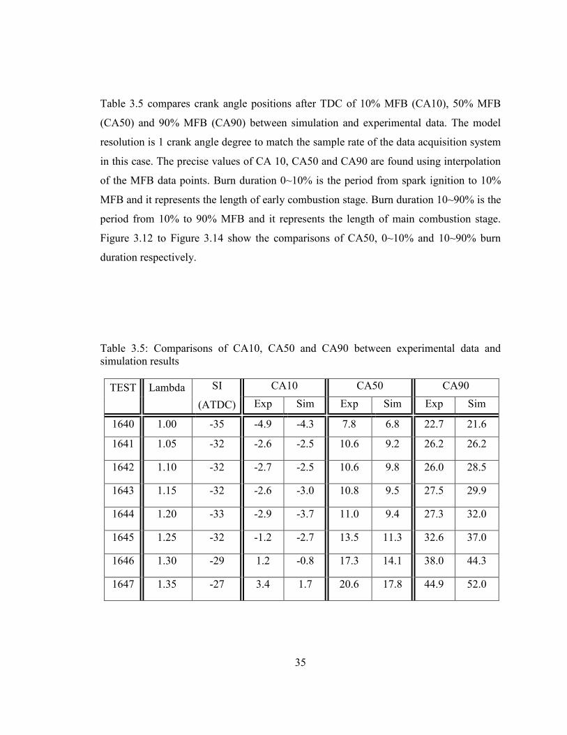
Table 3.5 compares crank angle positions after TDC of 10% MFB (CA10), 50% MFB

(CA50) and 90% MFB (CA90) between simulation and experimental data. The model

resolution is 1 crank angle degree to match the sample rate of the data acquisition system

in this case. The precise values of CA 10, CA50 and CA90 are found using interpolation

of the MFB data points. Burn duration 0~10% is the period from spark ignition to 10%

MFB and it represents the length of early combustion stage. Burn duration 10~90% is the

period from 10% to 90% MFB and it represents the length of main combustion stage.

Figure 3.12 to Figure 3.14 show the comparisons of CA50, 0~10% and 10~90% burn

duration respectively.

Table 3.5: Comparisons of CA10, CA50 and CA90 between experimental data and simulation results

TEST Lambda SI

(ATDC)

CA10 CA50 CA90 Exp Sim Exp Sim Exp Sim

1640 1.00 -35 -4.9 -4.3 7.8 6.8 22.7 21.6

1641 1.05 -32 -2.6 -2.5 10.6 9.2 26.2 26.2

1642 1.10 -32 -2.7 -2.5 10.6 9.8 26.0 28.5

1643 1.15 -32 -2.6 -3.0 10.8 9.5 27.5 29.9

1644 1.20 -33 -2.9 -3.7 11.0 9.4 27.3 32.0

1645 1.25 -32 -1.2 -2.7 13.5 11.3 32.6 37.0

1646 1.30 -29 1.2 -0.8 17.3 14.1 38.0 44.3

1647 1.35 -27 3.4 1.7 20.6 17.8 44.9 52.0

36

Figure 3.12: Comparison of CA50 values between simulation results and experimental data, tests 1640 to 1647 (lambda sweep).

Figure 3.13: Comparison of 0~10% burn duration values between simulation results and experimental data, tests 1640 to 1647 (lambda sweep).

37

Figure 3.14: Comparison of 10~90% burn duration values between simulation results and experimental data, tests 1640 to 1647 (lambda sweep).

From the comparisons in the table and figures, some conclusions could be made. Overall,

the simulation results of burn durations represent proper trend comparing with

experimental observations. The prediction of combustion model has better agreement

with experimental data when lambda is around 1 since parameters are tuned with

stoichiometric condition. The deviation increases while combustion becomes leaner. The

estimation errors for 0~10% burn durations are less than that of 10~90% burn duration.

38

4 STUDY CYCLIC VARIATION USING DEVELOPED COMBUSTION MODEL

As discussed in literature review, cycle-to-cycle variation exists in the combustion of IC

engines. The variation may be caused by several reasons. Except the variation of engine

operation conditions, some other variation sources in the combustion may exist. In this

chapter, the original variation sources are introduced in to complete the combustion

model and their influence is validated through the comparison of cyclic variation between

simulation results and that exists in experimental results.

4.1 CYCLICVARIATION IN ENGINE COMBUSTION

To analyze combustion variability, the test conditions, including intake manifold

pressure, temperature, spark, valve timing and fuel delivering amount are fixed in the

engine tests. The data starts to be recorded when the intake manifold and engine coolant

temperatures are stable. The electronic throttle position is fixed to maintain intake

pressure. The fuel injectors are controlled to deliver fuel with the amount based on the

intake air mass. Although all the test inputs are controlled with small amount of

variations, the variation of the observed in-cylinder pressure curves is substantial.

Figure 4.1 gives the time-based intake manifold pressures of 600 successive combustion

cycles captured by ACAP system. The pressure values have relative high fluctuation with

a mean value around 62.5 KPa. Figure 4.2 and Figure 4.3 show the cyclic variation of

intake pressure and MFB for the cylinder #1 in test 1640 (2000 rpm, 5 bar BMEP,

lambda = 1, MBT). Figure 4.4 and Figure 4.5 show the cyclic variation of intake pressure

and MFB in test 1647 (2000 rpm, 5 bar BMEP, lambda = 1.35). Comparing with these

figures, we can see that the cyclic variation is enlarged when engine runs leaner (lambda

= 1.35).

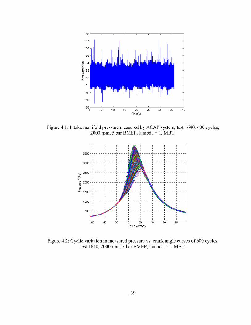
39

Figure 4.1: Intake manifold pressure measured by ACAP system, test 1640, 600 cycles, 2000 rpm, 5 bar BMEP, lambda = 1, MBT.

Figure 4.2: Cyclic variation in measured pressure vs. crank angle curves of 600 cycles, test 1640, 2000 rpm, 5 bar BMEP, lambda = 1, MBT.

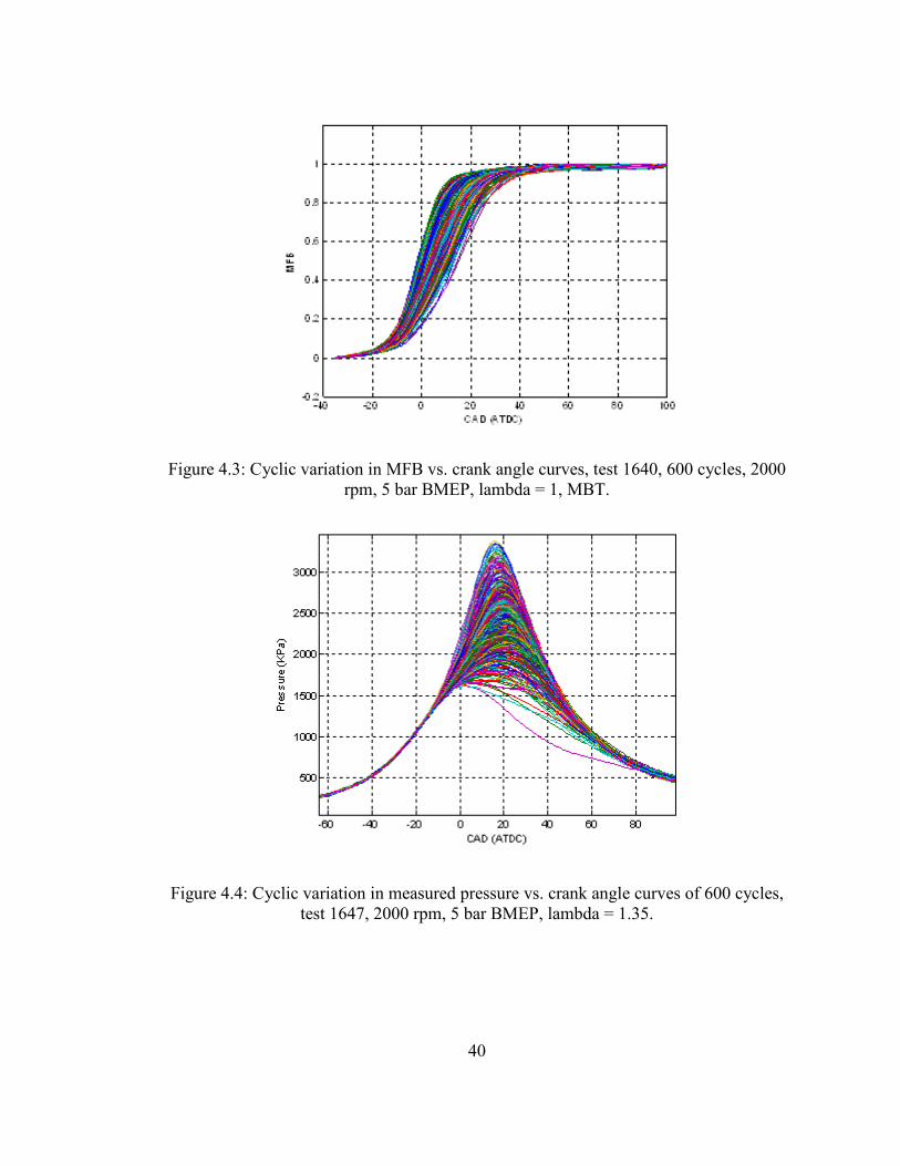
40

Figure 4.3: Cyclic variation in MFB vs. crank angle curves, test 1640, 600 cycles, 2000 rpm, 5 bar BMEP, lambda = 1, MBT.

Figure 4.4: Cyclic variation in measured pressure vs. crank angle curves of 600 cycles, test 1647, 2000 rpm, 5 bar BMEP, lambda = 1.35.

41

Figure 4.5: Cyclic variation in MFB calculated by measured data vs. crank angle curves of 600 cycles, test 1647, 2000 rpm, 5 bar BMEP, lambda = 1.35.

The cyclic variations are reflected in in-cylinder pressure and can be indicated by COV of

IMEP which is calculated by equation (33) [12]. Indicated mean effect pressure values

illustrate the effective work from the combustion of each cycle. It is the work produced in

each cycle divided by the clearance volume as shown in equation (34). The COV of

IMEP values of engine tests at different lean combustion levels are shown in Figure 4.6.

( )( ) 100%( )

std IMEPCOV IMEPavg IMEP

= × (33)

d

pdVIMEP

V= ∫ (34)

42

Figure 4.6: COV of IMEP vs. lambda from test results, test 1640 to 1647, average of 600 cycles, 2000 rpm, 5 bar BMEP, 0% EGR.

Figure 4.6 illustrates a very common phenomenon that the COV of IMEP keeps low near

lambda = 1 but increase rapidly when passing a certain lean point. From the combustion

burning process, the MFB curves in Figure 4.3 and Figure 4.5 show that the variation of

mass fraction burned appears from the start of combustion. The variation keeps

increasing during the progress of combustion. The analysis results in Ayala [1] reveal that

the periods from ignition to burning 10% of the mass (10% burn duration) obey a normal

distribution as shown in Figure 4.7 (a) and (b). The normal distribution demonstrates the

initial combustion variation nature. As the combustion continues, the variation of burning

duration becomes larger in amount and also gradually losses the symmetry. It is more

obvious in the case of high lean condition. For the advanced combustion cycles, their

deviations from average cycle are not large. However, for the retarded ones, their

deviations in early stage could lead worse and worse situation for fuel burning in the rest

of combustion period. In severe cases like the MFB curves in Figure 4.5, the partial mass

burning of some of the cycles may occur which will lead inefficient use of fuel.

43

(a)

(b)

(c)

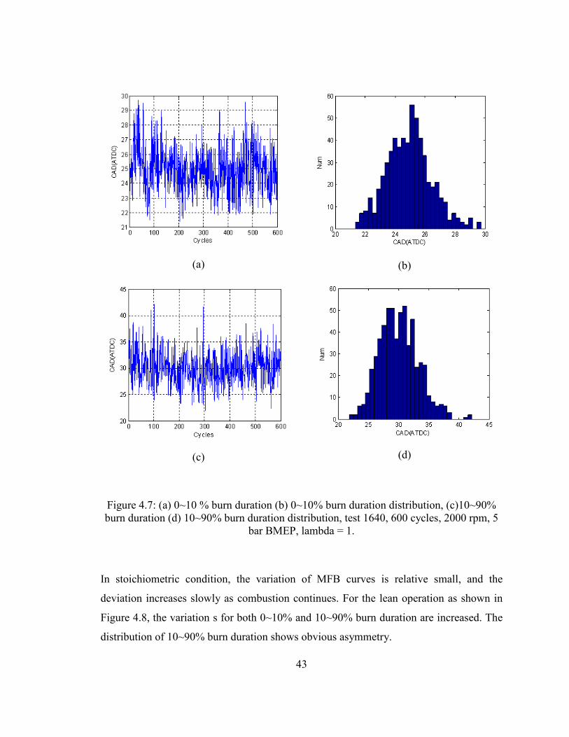
(d)

Figure 4.7: (a) 0~10 % burn duration (b) 0~10% burn duration distribution, (c)10~90% burn duration (d) 10~90% burn duration distribution, test 1640, 600 cycles, 2000 rpm, 5

bar BMEP, lambda = 1.

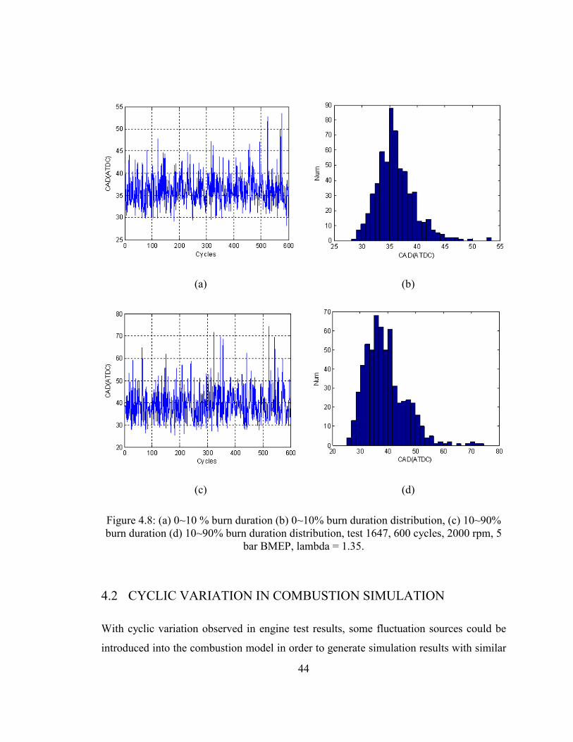
In stoichiometric condition, the variation of MFB curves is relative small, and the

deviation increases slowly as combustion continues. For the lean operation as shown in

Figure 4.8, the variation s for both 0~10% and 10~90% burn duration are increased. The

distribution of 10~90% burn duration shows obvious asymmetry.

44

(a)

(b)

(c)

(d)

Figure 4.8: (a) 0~10 % burn duration (b) 0~10% burn duration distribution, (c) 10~90% burn duration (d) 10~90% burn duration distribution, test 1647, 600 cycles, 2000 rpm, 5

bar BMEP, lambda = 1.35.

4.2 CYCLIC VARIATION IN COMBUSTION SIMULATION

With cyclic variation observed in engine test results, some fluctuation sources could be

introduced into the combustion model in order to generate simulation results with similar

45

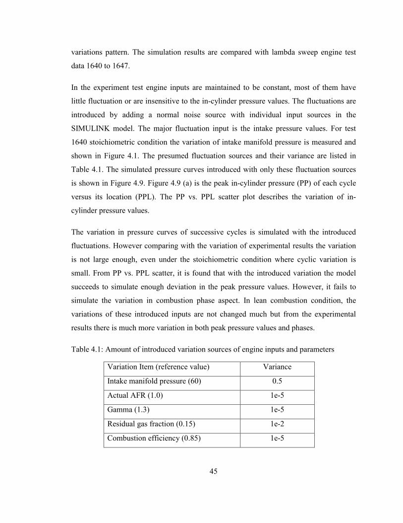
variations pattern. The simulation results are compared with lambda sweep engine test

data 1640 to 1647.

In the experiment test engine inputs are maintained to be constant, most of them have

little fluctuation or are insensitive to the in-cylinder pressure values. The fluctuations are

introduced by adding a normal noise source with individual input sources in the

SIMULINK model. The major fluctuation input is the intake pressure values. For test

1640 stoichiometric condition the variation of intake manifold pressure is measured and

shown in Figure 4.1. The presumed fluctuation sources and their variance are listed in

Table 4.1. The simulated pressure curves introduced with only these fluctuation sources

is shown in Figure 4.9. Figure 4.9 (a) is the peak in-cylinder pressure (PP) of each cycle

versus its location (PPL). The PP vs. PPL scatter plot describes the variation of in-

cylinder pressure values.

The variation in pressure curves of successive cycles is simulated with the introduced

fluctuations. However comparing with the variation of experimental results the variation

is not large enough, even under the stoichiometric condition where cyclic variation is

small. From PP vs. PPL scatter, it is found that with the introduced variation the model

succeeds to simulate enough deviation in the peak pressure values. However, it fails to

simulate the variation in combustion phase aspect. In lean combustion condition, the

variations of these introduced inputs are not changed much but from the experimental

results there is much more variation in both peak pressure values and phases.

Table 4.1: Amount of introduced variation sources of engine inputs and parameters

Variation Item (reference value) Variance

Intake manifold pressure (60) 0.5

Actual AFR (1.0) 1e-5

Gamma (1.3) 1e-5

Residual gas fraction (0.15) 1e-2

Combustion efficiency (0.85) 1e-5

46

(a) (b)

Figure 4.9: (a) Simulated pressure vs. crank angle curves (b) PP vs. PPL scatter, introduced with input fluctuations only, test 1640, 300 cycles, 2000 rpm, 5 bar BMEP,

lambda = 1.

To better match experimental data, additional fluctuation sources need to be considered.

Aghdam et al. [16] introduce fluctuation in turbulence into the fundamental combustion

model. The peak pressure vs. peak pressure location scatter matches that of experimental

result but the peak pressure points have too regular linear positions. In reality turbulent

flow has the variation nature. The turbulent flow structure is influenced by parameters

such as piston speed, mass density, pressure and temperature, so the turbulent level is

indirectly affected by lean combustion level. To further simulate the combustion

variation, the initial variations in the fuel burning speed and the early flame development

need to be considered.

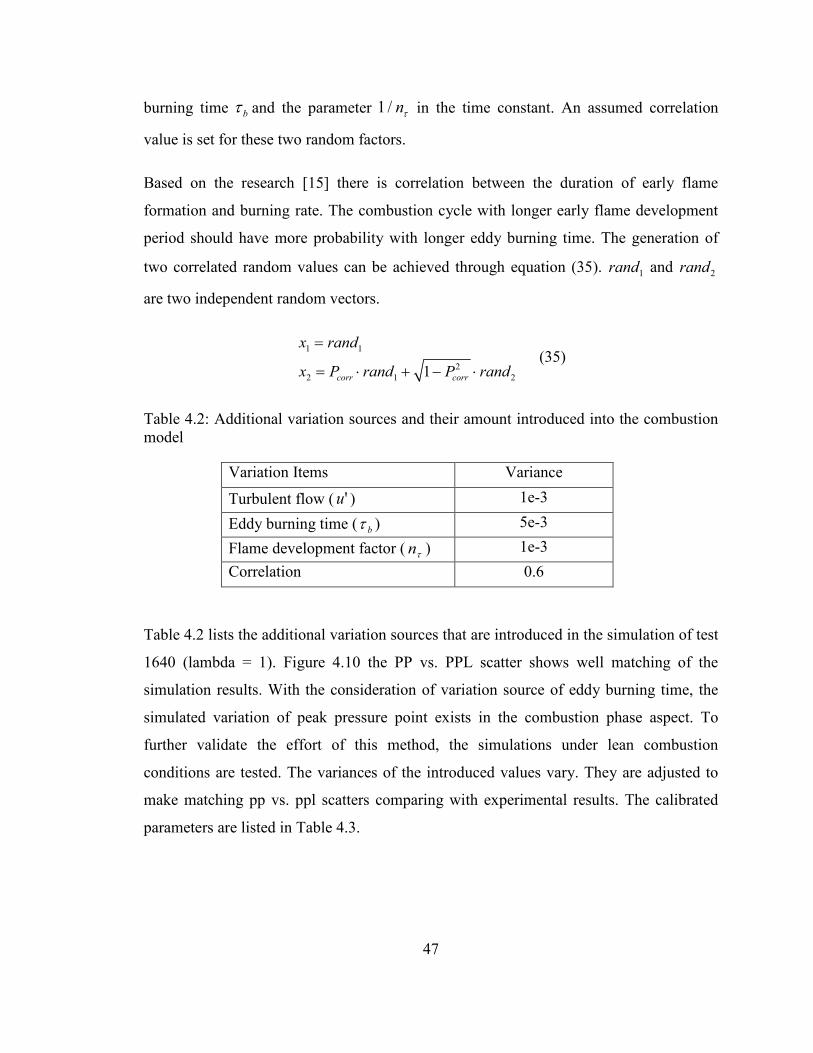
From the expressions of fundamental combustion model described previously, the

laminar burning speed ( LS ) and the eddy burning time ( bτ ), these parameters are related

to the fuel burning rate. The exponential factor with time constant ( b nττ ) related to eddy

burning time is used to express the growth of the early flame. In SIMULINK model the

introduction of variation is by adding normal noise sources to the calculations of eddy

47

burning time bτ and the parameter 1 / nτ in the time constant. An assumed correlation

value is set for these two random factors.

Based on the research [15] there is correlation between the duration of early flame

formation and burning rate. The combustion cycle with longer early flame development

period should have more probability with longer eddy burning time. The generation of

two correlated random values can be achieved through equation (35). 1rand and 2rand

are two independent random vectors.

1 1

22 1 21corr corr

x rand

x P rand P rand

=

= ⋅ + − ⋅ (35)

Table 4.2: Additional variation sources and their amount introduced into the combustion model

Variation Items Variance

Turbulent flow ( 'u ) 1e-3

Eddy burning time ( bτ ) 5e-3 Flame development factor ( τn ) 1e-3 Correlation 0.6

Table 4.2 lists the additional variation sources that are introduced in the simulation of test

1640 (lambda = 1). Figure 4.10 the PP vs. PPL scatter shows well matching of the

simulation results. With the consideration of variation source of eddy burning time, the

simulated variation of peak pressure point exists in the combustion phase aspect. To

further validate the effort of this method, the simulations under lean combustion

conditions are tested. The variances of the introduced values vary. They are adjusted to

make matching pp vs. ppl scatters comparing with experimental results. The calibrated

parameters are listed in Table 4.3.

48

Figure 4.10: PP vs. PPL scatters of simulation and experimental results, introduced with all fluctuation sources listed in Table 4.1 and Table 4.2 in simulation, test 1640, 600

cycles, lambda = 1.

Table 4.3: Variances of introduced variation sources under different lean conditions

Test 1640 1642 1645 1647

Lambda 1.0 1.1 1.25 1.35

Eddy burning time ( bτ ) 3e-3 5e-3 8e-3 1.5e-2

Flame development ( nτ ) 4e-3 4e-3 5e-3 5e-3

The simulation results of PP vs. PPL scatters in different lean combustion level are

shown in Figure 4.11 to Figure 4.13. Overall, the simulated variations in pressure match

well with those of experimental data except DC shift. The variances are calibrated by

comparing the variation in MFB curves with that of experimental results. From the

calibrated variance values, it is observed that the variance of eddy burning time ( bτ )

needs to be increased significantly as the lean level increases to make the simulation

result match. It can be concluded that the burning time in lean combustion condition is

49

not only large in average value but also has large variation which may be the major

impact factor of combustion stability.

Figure 4.11: PP vs. PPL scatters of simulation and experimental results, introduced with all fluctuation sources in simulation, test 1642, 600 cycles, lambda = 1.1.

50

Figure 4.12: PP vs. PPL scatters of simulation and experimental results, introduced with all fluctuation sources in simulation, test 1645, 600 cycles, lambda = 1.25.

Figure 4.13: PP vs. PPL scatters of simulation and experimental results, introduced with all fluctuation sources in simulation, test 1647, 600 cycles, lambda = 1.35.

51

The 0~10% and 10~90% burn durations of simulation results and experimental data are

also compared. For stoichiometric case the simulated and experimental MFB curves of

600 cycles are shown in Figure 4.14. For the lean condition, the MFB curves of 600

cycles under the highest lean condition that in comparison are shown in Figure 4.15. The

cyclic variation in simulated MFB results is calibrated to imitate that of experimental

MFB curves by adjusting the variances added on flame development rate ( nτ ) and eddy

burning time ( bτ ) shown in Table 4.3. The early MFB distribution range is affected by

both variations of nτ and bτ . The main MFB distribution range is affected by the

variation of bτ . From the MFB history curves the simulated variation in MFB is similar

to experimental ones. The detail distribution can be reflected by the comparison of burn

duration distribution. The comparisons of burn duration distribution of stoichiometric and

severe lean cases are shown in Figure 4.16 and Figure 4.17 separately.

(a)

(b)

Figure 4.14: (a) MFB curves of simulation results (b) MFB curves of experimental data, 600 cycles, 2000 rpm, 5 bar, lambda = 1.0.

52

(a)

(b)

Figure 4.15: (a) MFB curves of simulation results (b) MFB curves of experimental data, 600 cycles, 2000 rpm, 5 bar, lambda = 1.35.

53

(a)

(b)

(c)

(d)

Figure 4.16: (a) Distribution of 0~10% burn duration of simulation results (b) distribution of 0~10% burn duration of experimental data (c) distribution of 10~90 burn duration of simulation results (d) distribution of 10~90% burn duration of experimental data, 600

cycles, 2000 rpm, 5 bar, lambda = 1.0.

54

(a)

(b)

(c)

(d) Figure 4.17: (a) Distribution of 0~10% burn duration of simulation results (b) distribution of 0~10% burn duration of experimental data (c) distribution of 10~90 burn duration of simulation results (d) distribution of 10~90% burn duration of experimental data, 600

cycles, 2000 rpm, 5 bar, lambda = 1.35.

In stoichiometric case, the distribution of simulated MFB has high similarity with

experimental data in early stage (0~10% burn duration in Figure 4.16 (a) and (b)).

However, the 10~90% burn duration distribution from simulation has larger average

value and range than that of experimental data shown in Figure 4.16 (c) and (d). That

may be caused by the simulation error in the end part of MFB curves during combustion.

In lean condition, the 0~10% burn duration is not as concentrated as the experimental

distribution shown in Figure 4.17 (a) and (b). The range of 10~90% burn duration

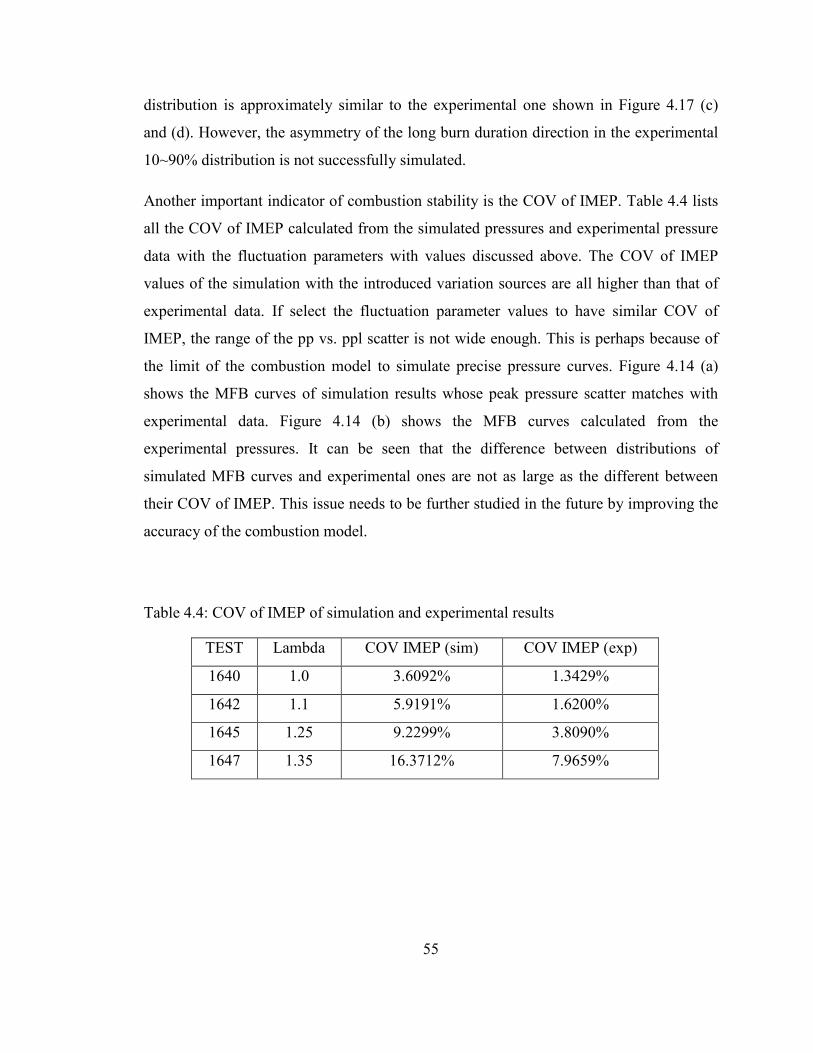
55

distribution is approximately similar to the experimental one shown in Figure 4.17 (c)

and (d). However, the asymmetry of the long burn duration direction in the experimental

10~90% distribution is not successfully simulated.

Another important indicator of combustion stability is the COV of IMEP. Table 4.4 lists

all the COV of IMEP calculated from the simulated pressures and experimental pressure

data with the fluctuation parameters with values discussed above. The COV of IMEP

values of the simulation with the introduced variation sources are all higher than that of

experimental data. If select the fluctuation parameter values to have similar COV of

IMEP, the range of the pp vs. ppl scatter is not wide enough. This is perhaps because of

the limit of the combustion model to simulate precise pressure curves. Figure 4.14 (a)

shows the MFB curves of simulation results whose peak pressure scatter matches with

experimental data. Figure 4.14 (b) shows the MFB curves calculated from the

experimental pressures. It can be seen that the difference between distributions of

simulated MFB curves and experimental ones are not as large as the different between

their COV of IMEP. This issue needs to be further studied in the future by improving the

accuracy of the combustion model.

Table 4.4: COV of IMEP of simulation and experimental results

TEST Lambda COV IMEP (sim) COV IMEP (exp)

1640 1.0 3.6092% 1.3429%

1642 1.1 5.9191% 1.6200%

1645 1.25 9.2299% 3.8090%

1647 1.35 16.3712% 7.9659%

56

4.3 COMBUSTION STABILITY ANALYSIS

For the lean combustion conditions, the burning duration is enlarged because of the slow

laminar burning speed. The heat release has more space to vary because of the longer

combustion duration. Another major cause of combustion stability should be the variation

during the early flame formation, in which the laminar speed is the major part of flame

propagation. The simulation results show the probability of large amount of variation in

the early combustion under lean conditions. Comparing the MFB curves in Figure 4.3

and Figure 4.5, it is found that is much larger in lean condition (lambda = 1.35).

Figure 4.3 and Figure 4.5 show the variations in MFB curves of stoichiometric and lean

(lambda = 1.35) conditions. The stoichiometric MFB curves have better stability. Most of

stoichiometric combustion have short burn duration and the phase located around MBT

point with CA50 around 7~9 deg ATDC. On the other hand, the MFB curves in lean

conditions are worse in stability. A lot of them have late phase and slow burning rate.

To study the effect of cyclic variation causes, the calibrated variance value of the flame

development variation source in the lean condition (lambda = 1.35) is included for the

simulation in the stoichiometric condition. Figure 4.18 (a) shows the MFB results of the

simulation and the experimental MFB curves are shown in Figure 4.18 (b). Similarly, the

variance value of eddy burning time calibrated in stoichiometric condition is introduced

in the simulation of lean combustion condition (lambda = 1.35). Figure 4.19 (a) shows

the simulation results and the experimental MFB curves of lean condition (lambda =

1.35) are shown in Figure 4.19 (b). From the results of the first simulation, it is found that

even though with large variation in the early stage of combustion, stoichiometric

condition provides relatively fast burning environment which restricts the growth of

deviation. In the second simulation, even though under the severe lean combustion

condition, the MFB curves concentrate while combustion proceeding and the very late

and partial burn cycles are avoided.

57

(a) (b)

Figure 4.18: (a) MFB curves of simulation introduced with large variance in early flame burning (b) experimental data, test 1640, 600 cycles, lambda = 1.

(a) (b)

Figure 4.19: (a) MFB curves of simulation introduced with small variance in eddy burning time (b) experimental result, test 1647, 600 cycles, lambda = 1.35.

58

The combustion efficiency is also studied for stable combustion. Spark-ignition engines

achieve the maximum efficiency when spark ignition is set at the MBT point. The MBT

cycle has the pressure versus chamber volume curve most similar to that of ideal

combustion model. The ideal combustion cycle of SI engine uses that all of the energy

from fuel releases at the TDC point to raise in-cylinder pressure. The cycles that vary

from the MBT cycle have lower efficiency [12].

An indicator of combustion efficiency or fuel economy is the specific fuel consumption

(sfc) expressed in equation (36). In the presented combustion model, sfc of each cycle is

calculated with the fuel mass estimated by intake pressure, temperature and the actual

AFR etc.

fmsfc

Power=

(36)

By choosing the optimal spark ignition timing the combustion could be controlled in

MBT phase. Most of the cycles could operate around MBT phase if the combustion is

stable. For combustion with large variation, the phases of more cycles are deviated from

the required MBT phase. Consequently the efficiency loss increases when the variation

becomes large. Figure 4.20 to Figure 4.23 show the sfc distributions from simulation

results under different lean combustion conditions. The sfc values of most cycles locate

on the left side of the distribution in stable combustion condition. Only small amount of

cycles have large differences. However, in the lean combustion condition, the number of

cycles with large sfc values increases and also their deviations from the lowest sfc cycle

is increased. Comparing these figures the width of the distribution range increases as the

increasing of lean combustion level.

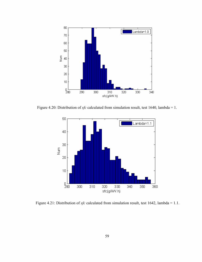
59

Figure 4.20: Distribution of sfc calculated from simulation result, test 1640, lambda = 1.

Figure 4.21: Distribution of sfc calculated from simulation result, test 1642, lambda = 1.1.

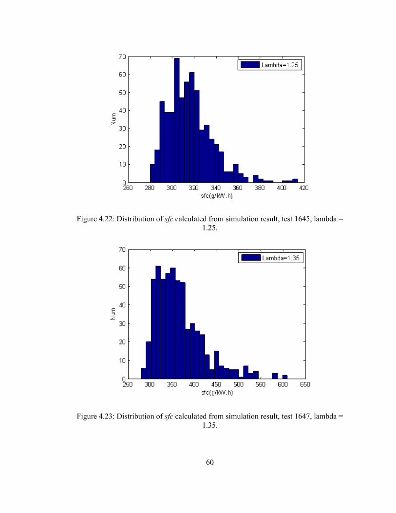
60

Figure 4.22: Distribution of sfc calculated from simulation result, test 1645, lambda = 1.25.

Figure 4.23: Distribution of sfc calculated from simulation result, test 1647, lambda = 1.35.

61

5 CONCLUSIONS AND FUTURE WORKS

A zero-dimensional fundamental combustion model proposed by several authors is

studied and implemented in Simulink to simulate in-cylinder pressure for a Ford

Ecoboost 3.5L central ignited SI engine. The combustion process is described as

turbulent flame propagation and large eddy burning with laminar flame speed. With

assumption of spherical flame geometry and using two-zone thermodynamic model, the

presented combustion model is able to predict mass density temperature and pressure

variables. The simulation results of in-cylinder pressure and MFB are approximately

matched with engine experimental data under various operation conditions.

The cyclic variation of consecutive combustion cycles exists in in-cylinder pressure

traces. This variation increases when an engine operates in leaner combustion conditions.

This phenomenon could be simulated by introducing variation sources of engine

parameters, eddy burning time and the early flame development rate. The variance values

are chosen to make peak pressure scatter match that of experimental result. The calibrated

variation values of different lean level simulations reveals that the variations of eddy

burning time and early flame development rate increase in lean combustion conditions.

Cyclic variation caused by the early deviation and growth during the long combustion

period leads efficiency losses due to the wide range of sfc distribution.

For the future work, physical explanations of fuel economy increase before the lean limit

can be explored with the combustion model. Further analysis needs more capable

combustion model. The combustion model includes laminar flame speed in the flame

propagation. Actually simulation result shows dominant turbulent propagation speed

from very start of combustion. The effect of laminar flame speed in the early flame

formation needs to be studied and evolved into the combustion model. In addition, the

presented model needs to be validated with experimental data of more operation

conditions. More detail of engine conditions such as residual gas fraction and ignition

process could be considered in the simulation. The presented combustion model also

needs to be modified to simulate more precise mass burn rate and in-cylinder pressure in

lean combustion conditions. The eddy burning rate during the last half of combustion

62

needs to be refined to predict more precise mass burning rate values. The amounts of

variation sources introduced in the multi-cycle simulation under different lean levels need

to be quantified. Comparisons of other combustion matrices and under more operation

conditions are needed. And also further study of the variation source and amounts

introduced in the model is needed to simulate the asymmetry of 10~90% burn duration

distribution under lean conditions.

63

REFERENCES

1. Ayala, F.A. and J.B. Heywood, Lean SI Engines: The role of combustion variability in defining lean limits. 2007, Consiglio Nazionale delle Ricerche.

2. Rhodes, D.B. and J.C. Keck, Laminar Burning Speed Measurements of Indolene-Air-Diluent Mixtures at High Pressures and Temperatures. 1985, SAE International.

3. Keck, J.C., Turbulent flame structure and speed in spark-ignition engines. Symposium (International) on Combustion, 1982. 19(1): p. 1451-1466.

4. Wong, V.W. and D.P. Hoult, Rapid Distortion Theory Applied to Turbulent Combustion. 1979, SAE International.

5. Keck, J.C., J.B. Heywood, and G. Noske, Early Flame Development and Burning Rates in Spark Ignition Engines and Their Cyclic Variability. 1987, SAE International.

6. Blizard, N.C. and J.C. Keck, Experimental and Theoretical Investigation of Turbulent Burning Model for Internal Combustion Engines. 1974, SAE International.

7. Tabaczynski, R.J., C.R. Ferguson, and K. Radhakrishnan, A Turbulent Entrainment Model for Spark-Ignition Engine Combustion. 1977, SAE International.

8. Tabaczynski, R.J., F.H. Trinker, and B.A.S. Shannon, Further refinement and validation of a turbulent flame propagation model for spark-ignition engines. Combustion and Flame, 1980. 39(2): p. 111-121.

9. Ayala, F.A. and Massachusetts Institute of Technology. Department of Mechanical Engineering., Combustion lean limits fundamentals and their application to a SI hydrogen-enhanced engine concept. 2006. p. 205 p.

10. Guezennec, Y.G. and W. Hamama, Two-Zone Heat Release Analysis of Combustion Data and Calibration of Heat Transfer Correlation in an I. C. Engine. 1999, SAE International.

11. Ayala, F.A., M.D. Gerty, and J.B. Heywood, Effects of Combustion Phasing, Relative Air-fuel Ratio, Compression Ratio, and Load on SI Engine Efficiency. 2006, SAE International.

12. Heywood, J.B., Internal combustion engine fundamentals. 1988, New York: McGraw-Hill. xxix, 930 p.

13. Beretta, G.P., M. Rashidi, and J.C. Keck, Turbulent Flame Propagation and Combustion in Spark-Ignition Engines. Combustion and Flame, 1983. 52(3): p. 217-245.

14. Yeliana, et al., The Calculation of Mass Fraction Burn of Ethanol-Gasoline Blended Fuels Using Single and Two-Zone Models. 2008, SAE International.

15. Rashidi, M., The nature of cycle-by-cycle variation in the S.I. Engine from high speed photographs. Combustion and Flame, 1981. 42(0): p. 111-122.

16. Abdi Aghdam, E., et al., Study of Cyclic Variation in an SI Engine Using Quasi-Dimensional Combustion Model. 2007, SAE International.

17. Tennekes, H. and J.L. Lumley, A first course in turbulence. 1972, Cambridge, Mass.,: MIT Press. xii, 300 p.

64

18. Woschni, G., A Universally Applicable Equation for the Instantaneous Heat Transfer Coefficient in the Internal Combustion Engine. 1967, SAE International.

19. Fox, J.W., W.K. Cheng, and J.B. Heywood, A Model for Predicting Residual Gas Fraction in Spark-Ignition Engines. 1993, SAE International.

20. Robert Bosch GmbH., Gasoline-engine management. 2nd ed. 2004, Bury St Edmunds: Professional Engineering. 418 p.

65

APPENDIX A

MATLAB SCRIPTURE OF COMBUSTION MODEL SETUP

%% SETUP FOR COMBUSTION MODEL SIMULATION IN SIMULINK % % Hao Wu % clear all; close all; clc; load V_CA.mat; % load volume [L], crank angle [deg] %% Load Engine Data %%SI sweep, 1500 rpm, 2.62 bar, TEST1019~1031 20%EGR, 1240~1255 0%EGR % load('../../SI_sweep_result/TEST1240.mat'); %%Lambda sweep, 2000 rpm, 5 bar, TEST 1640~1648 load('../../lambda_sweep_result/TEST1647.mat'); %%EGR sweep, 1000 rpm, 1.5 bar, TEST 995~1003 % load('../../EGR_sweep_result/TEST997.mat'); %%Other data % load('../../../EGR_sweep/other_result/2000_2_0.mat','Prf','SI','CA100'); IND = 1:600; %% INPUTS NN = length(IND); % cycle number N = 2000; % engine speed [rpm] P_in = 66.3832; % intake manifold pressure % BMEP = 5; % BMEP [bar] EGR = 0; % EGR [%] lambda = 1.0; dt = 60/N/360; % sample rate CA = -179:540; % crank angle (dATDC) SI = -35; % spark ignition %% LOOKUP TABLE lambda_map = 1.0:0.05:1.35; n_c = [0.85 0.85 0.87 0.91 0.93 0.95 0.95 0.95]; load air_voscosity_converge.mat; % Mu_0 vs. T_0 %% GENERAL PARAMETERS Ti = 358; % intake manifold temperature [K] R = 0.287; % pV = mRT [KJ/(kg.K)] %% ENGINE PARAMETERS AFR_stoi = 14.6; % 14.6 rc = 1.31; % heat capacity ratio, compression stroke re = 1.26; % heat capacity ratio, expansion stroke nc = rc; % compression polytropic coeff; ne = re; % expansion polytropic coeff; cv_u = 0.72; % [KJ/(kg.K)]

66

cv_b = 0.8; % [KJ/(kg.K)] IVC = 10 - 180; % intake value close, dABDC EVO = 0 +180; % exhaust value open, dABDC IVO = 320 +180; % intake value open, dABDC LHV = 44*1000; % lower heating value [J/g] T_wall = 360; % wall (coolant) temperature %% GEOMETRY PARAMETERS L = 0.0867; % length of stroke [m] B = 0.0925; % length of bore [m] l = 0.15268; % connecting rod length [m] CR = 10; % compression ratio Vd = 3.496; % displacement [L] H = V/(pi*(B*1000/2)^2)*1e6; % distance between pistion head to cylinder head [mm] %% VARIATIONS var_Ti = 0; var_Pi = 0.5; var_lambda = 1e-5; var_N = 0; var_n_c = 1e-5; var_res = 1e-2; var_gamma = 1e-5; var_const1 = 1e-3; var_const = 0; var_lambda1 = 2e-2; var_SL = 5e-3; var_SI = 0; %% SEEDS seed_lambda1 = round(rand(1)*1e3); seed_SL = round(rand(1)*1e3); p_corr = 0.6; %% MODEL PARAMETERS %%assumption res = 15; % residual [%] %%Heat transfer c_ht = 0.008; % constant of heat transfer coefficient %%model parameters const1 = 1.8; u0_ind = 1/6; const2 = 1; % u constant const = 16.5; % constant of Taylor microscale lambda_m lambda1 = 5; % tao_b/lambda1 %%For laminar speed SL n = 2; fn_a = 4.70617; fn_b = -4.06185; %% RUN SIMULATION sim('combustion_model_simulation.mdl'); %% PLOT simulation_results;

67

APPENDIX B

GRAPIC PROGRAM OF COMBUSTION MODEL IN SIMULINK ENVIRONMENT

Appendix 1: First layer of fundamental combustion model in SIMULINK graphic design environment.