Study of Positronium Converters in the AEGIS Antimatter Experiment
103
UNIVERSITÀ DEGLI STUDI DI MILANO SCUOLA DI DOTTORATO FISICA, ASTROFISICA E FISICA APPLICATA DIPARTIMENTO DI FISICA CORSO DI DOTTORATO DI RICERCA IN FISICA, ASTROFISICA E FISICA APPLICATA CICLO XXIII Study of Positronium Converters in the AEGIS Antimatter Experiment Settore Scientifico disciplinare FIS/04 Tesi di Dottorato di: Davide Trezzi Supervisore: Dott. Marco Giulio Giammarchi Coordinatore: Prof. Marco Bersanelli A.A. 2009-2010
Transcript of Study of Positronium Converters in the AEGIS Antimatter Experiment
UNIVERSITÀ DEGLI STUDI DI MILANO
SCUOLA DI DOTTORATO FISICA, ASTROFISICA E FISICA APPLICATA
DIPARTIMENTO DI FISICA
CORSO DI DOTTORATO DI RICERCA IN FISICA, ASTROFISICA E FISICA APPLICATA
CICLO XXIII
Study of Positronium Converters in the AEGIS Antimatter Experiment
Settore Scientifico disciplinare FIS/04
Tesi di Dottorato di: Davide Trezzi Supervisore: Dott. Marco Giulio Giammarchi Coordinatore: Prof. Marco Bersanelli
A.A. 2009-2010
Contents
1 AEgIS antimatter experiment, an overview 31.1 The theoretical framework . . . . . . . . . . . . . . . . . . . . 31.2 Antihydrogen Physics . . . . . . . . . . . . . . . . . . . . . . 41.3 The AEgIS experiment . . . . . . . . . . . . . . . . . . . . . . 5
1.3.1 Production of cold anti-hydrogen . . . . . . . . . . . . 51.3.2 Formation and acceleration of anti-hydrogen beam . . 61.3.3 Measurement of the gravitational acceleration . . . . . 7
2 The AEgIS positron source 82.1 The positron source . . . . . . . . . . . . . . . . . . . . . . . 82.2 The moderator system . . . . . . . . . . . . . . . . . . . . . . 102.3 The positron magnetic guide . . . . . . . . . . . . . . . . . . 112.4 The RGM system . . . . . . . . . . . . . . . . . . . . . . . . . 15
3 Positronium Physics 173.1 Introduction . . . . . . . . . . . . . . . . . . . . . . . . . . . . 173.2 Positronium formation in solids . . . . . . . . . . . . . . . . . 18
3.2.1 Positronium formation in metal and semiconductors . 183.2.2 Positronium formation in insulators . . . . . . . . . . 193.2.3 Monte Carlo simulation of Ps formation in solids . . . 193.2.4 Positronium thermalization in porous media . . . . . . 24
3.3 Positronium detection . . . . . . . . . . . . . . . . . . . . . . 253.3.1 Positron Annihilation Lifetime Spectroscopy . . . . . . 253.3.2 Technical application: effects of the oPs formation in
organic liquid scintillators on electron anti-neutrinodetection . . . . . . . . . . . . . . . . . . . . . . . . . 30
3.3.3 Determination of ortho-positronium yield formation . 373.4 Positronium converter in AEgIS . . . . . . . . . . . . . . . . 40
3.4.1 Metal/SiO2 Microspheres . . . . . . . . . . . . . . . . 423.4.2 Whatman R© membrane . . . . . . . . . . . . . . . . . . 433.4.3 Vycor glass . . . . . . . . . . . . . . . . . . . . . . . . 443.4.4 MOFs . . . . . . . . . . . . . . . . . . . . . . . . . . . 443.4.5 Aerogel/Xerogel . . . . . . . . . . . . . . . . . . . . . 45
1
CONTENTS 2
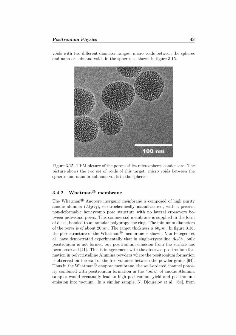
3.4.6 MACS . . . . . . . . . . . . . . . . . . . . . . . . . . . 463.4.7 Ordered nano-channels Si/SiO2 . . . . . . . . . . . . 473.4.8 Conclusions . . . . . . . . . . . . . . . . . . . . . . . . 48
3.5 Positronium formation in extreme conditions . . . . . . . . . 51
4 Electron beam for ageing measurements 534.1 eBEAM apparatus . . . . . . . . . . . . . . . . . . . . . . . . 534.2 The electron source . . . . . . . . . . . . . . . . . . . . . . . . 57
4.2.1 TES-eBEAM . . . . . . . . . . . . . . . . . . . . . . . 574.2.2 ES-eBEAM . . . . . . . . . . . . . . . . . . . . . . . . 62
4.3 The magnetic guide field . . . . . . . . . . . . . . . . . . . . . 654.4 The sample support . . . . . . . . . . . . . . . . . . . . . . . 674.5 Acquisition system . . . . . . . . . . . . . . . . . . . . . . . . 674.6 Ageing measurements . . . . . . . . . . . . . . . . . . . . . . 73
5 Conclusions 74
A Thermionic emission from tungsten wire 76A.1 Introduction . . . . . . . . . . . . . . . . . . . . . . . . . . . . 76A.2 The energy spectrum of the thermionically emitted electrons 78A.3 A Monte Carlo simulation of thermionic emission from Tung-
sten wire . . . . . . . . . . . . . . . . . . . . . . . . . . . . . . 79
B The eBEAM magnetic field 83B.1 Magnetic field calculation . . . . . . . . . . . . . . . . . . . . 83
B.1.1 Introduction . . . . . . . . . . . . . . . . . . . . . . . 83B.1.2 MI-AEGIS.Mag . . . . . . . . . . . . . . . . . . . . . . 85B.1.3 MI-AEGIS.Mag experimental test . . . . . . . . . . . 88B.1.4 Magnetic field map implementation in SIMION R© . . . 88
B.2 A gaussmeter design for the eBEAM apparatus. . . . . . . . . 91
Bibliography 91

Chapter 1
AEgIS antimatterexperiment, an overview
1.1 The theoretical framework
The theory that describes the gravitational interaction is General Relativity,formulated by A. Einstein in 1915. This theory is based on the equivalenceprinciple that, in its original formulation, assumes the physical equivalencebetween gravitational field and an uniform accelerating reference frame. To-day we have three formulations for the equivalence principle, namely: theweak equivalence principle, Einstein’s equivalence principle and the strongequivalence principle. The last two require the veridicity of the first one, thatis: “all bodies in the same time-space point, in a given gravitational field,are subject to the same acceleration”. In the particle physics framework thismeans that matter and antimatter in the same gravitational field, like theEarth’s one, should be subject to the same acceleration or the gravitationalinteraction is unchanged under charge conjugation symmetry. Modern the-ories [1] (e.g theories of supergravity), formulated in order to unify in onetheory the gravitational interaction with the electroweak and strong inter-actions, allow for the possibility that matter and antimatter can interact ina different way in some gravitational field, and in particular in the terrestialone. In other words, this would result in the violation of the weak equiva-lence principle. An experimental evidence is thus fundamental in order totest such candidate theory of everything.
In the formalism of modern quantum mechanics, every local Lorentz-invariant quantum field theory, like the Particle Standard Model, should beinvariant under CPT transformation that is the composition of three dis-crete symmetries: charge conjugation C, parity P and time reversal T. Thisproperty was independently found by G. Luders, W. Pauli and J. Schwingerand is nowadays known as the CPT theorem [2]. From CPT theorem onecan derive some interesting conclusions:
3
AEgIS antimatter experiment, an overview 4
1. particles can follow Bose-Einstein or Fermi-Dirac statistics. If theyhave integer spin they follow the Bose-Einstein statistics otherwise inthe case of semi-integer spin, they follow the Fermi-Dirac statistics. Inquantum mechanics this imply that the integer spin operators shouldbe quantized using the commutation rules whereas the semi-integerones should be quantized using the anti-commutation rules;
2. particles and anti-particles must have identical rest masses and life-times;
3. all internal quantum numbers of the anti-particles must be oppositethan those of the corresponding particle;
4. the transition frequencies for the matter and anti-matter bound statesmust be the same.
While experimental P,C,CP and T symmetries (in the Particle StandardModel) are violated [3], CPT violations have never been found. The im-portance of this symmetry requires accurate experimental tests with everykind of particles: barions, mesons and leptons. AEgIS - namely AntimatterExperiment: Gravity, Interferometry, Spectroscopy [4] - is an experiment de-signed to test the weak equivalence principle by measuring the g constantwith an accuracy of about 1% for anti-hydrogen atoms. Moreover, grav-ity measurements should be indipendent from the theoretical frameworkused to describe the interaction with the Earth’s gravitational field. In asecond phase of the experiment, a comparison between the hydrogen andanti-hydrogen electromagnetic spectrum will give a high sensitivity test forthe CPT theorem.
1.2 Antihydrogen Physics
Antihydrogen is the simplest antimatter atoms. It is composed of an an-tiproton and positron (anti-electron). The first evidence of antihydrogenwas obtained at CERN in 1995. The experiment, named PS210 [5], tookplace in the LEAR antiproton ring facility [6] where antiprotons, producedin the PS ring [7], hit Xenon atoms in order to produce electron-positronpairs. Thus antiprotons and positrons could form antihydrogen atoms butwith high mean kinetic energy (billions of Kelvin (∼ GeV , indicated like”hot antihydrogen”). Hot antihydrogen production was confirmed later, in1997, at Fermilab accelerator [8]. Antihydrogen of such high energy couldnot be used for tests of fundamental symmetries. In 2000, the AD Antipro-ton Decelerator ring [9] substitute the older LEAR, in order to decelerateantiproton to 5MeV . The new energy of the antiproton beam can be furtherdecelerate to a few eV after moderation. Two AD experiments, ATRAP [10]and ATHENA [11], brought together antiprotons and positrons (produced
AEgIS antimatter experiment, an overview 5
by a Sodium 22 radioactive source) in Penning traps. Such antihydrogenatoms, produced for the first time by ATHENA [12] and subsequently byATRAP [13] in 2002, had a mean kinetic energy of a hundred Kelvin. Theseatoms are still too hot to be used for experiments like atomic spectroscopy.However ATHENA and ATRAP gave the first evidence that cold antihy-drogen could be made. A new experiment, ALPHA[14], as well as ATRAP,is pursuing the production of antihydrogen at much lower kinetic energyso that it could be confined magnetically. In 2008 the AEgIS experiment[15] proposed another process - namely the charge exchange reaction be-tween antiproton and positronium - in order to produce ”cold antihydrogen”with a mean kinetic energy of the order of 100mK. Such low energy beamwill be used for gravity fall measurements (see the next sections). Otherexperiments at CERN are using antihydrogen for antimatter physics, likeASACUSA [16] (Atomic spectroscopy and collisions using slow antiprotons)and ACE [17] (Relative biological effectiveness and peripheral damage ofantiproton annihilation).
1.3 The AEgIS experiment
The AEgIS experiment, under construction at the CERN Antiproton De-celerator1, aims at directly measuring the gravitational acceleration g bydetecting the vertical deflection of an anti-hydrogen beam, after a flightpath of about 1 meter, with a 1% relative precision. In AEgIS , the essentialsteps leading to the production of anti-hydrogen (H) and the measurementof gravitational interaction it undergoes are:
1. the production of cold (100mK) anti-hydrogen beam based on thecharge exchange reaction between cold (100mK) anti-protons and Ry-dberg positronium,
2. the formation and acceleration of a Rydberg anti-hydrogen beam usinginhomogeneous electric fields and
3. the determination of g through the measurement of the vertical deflec-tion of the antihydrogen beam in a two-grating Moire deflectometercoupled with a position-sensitive detector.
1.3.1 Production of cold anti-hydrogen
Cold anti-hydrogen (H) in AEgIS will be produced by the charge exchangereaction between cold anti-protons (p) and Rydberg positronium (Ps∗):
p+ Ps∗ → H∗ + e−
1The experiment has been approved at CERN in 2008 and the installation in theexperimental hall has begun in 2010.
AEgIS antimatter experiment, an overview 6
Antiprotons delivered by the CERN Antiproton Decelerator, will be trappedin a Malmberg-Penning trap (catching trap) mounted in a horizontal cryo-stat inside the bore of a 3 Tesla magnetic field and cooled by electron coolingdown to subeV energies in a cryogenic environment at 4K in temperature.The antiproton cloud will be radially compressed and then transferred into asecond trap mounted in a colder region (100 mK) and with a magnetic fieldof 1 Tesla (antihydrogen formation trap). Here antiprotons will be cooleddown to 100 mK.
Instead, the Positronium will be formed by bombarding a porous mate-rial - converter - with bunches of 108 positrons, with a time length of 10-20ns. A fraction of the positrons are re-emitted as positronium atoms with avelocity of about 104m/s. In this thesis we will investigate the propriertiesof the AEgIS candidate converters. Positronium atoms are subsequentiallyexcited, by two laser pulses, to Rydberg states with principal quantum num-ber n = 20 − 30, thus optimizing the cross section of the charge exchangereaction which depends on the fourth power of n [15].
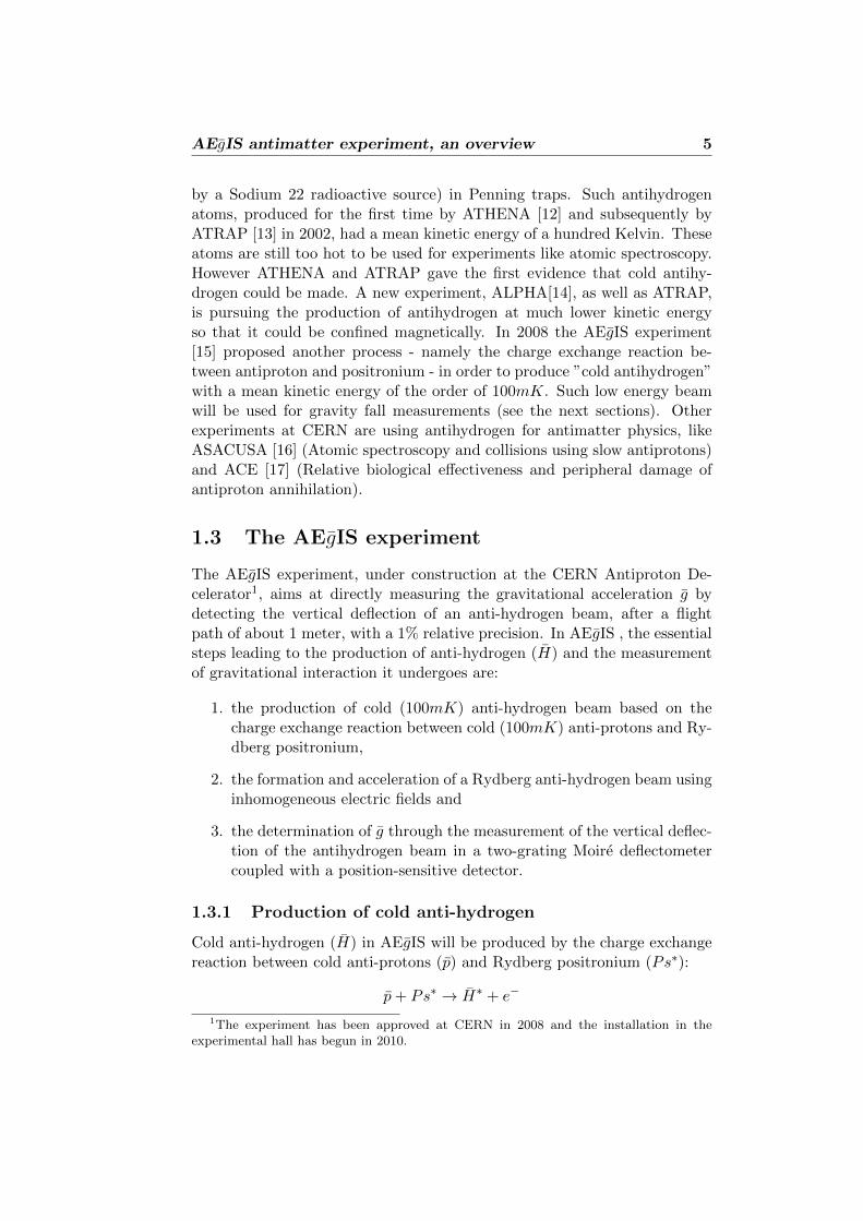
The production of cold (100mK) anti-hydrogen takes place when theRydberg positronium traverses the cold anti-proton cloud. Taking into ac-count the velocity of the Rydberg positronium and the anti-proton clouddimensions (of the order of few mm) the production time of anti-hydrogenis defined within about 1µs. This pulsed anti-hydrogen production allowsfor the possibility of measuring both the anti-hydrogen temperature and theg constant, by a time of flight method. Figure 1.1 shows the region whereanti-hydrogen will be formed, accelerated and sent to the grating system.
1.3.2 Formation and acceleration of anti-hydrogen beam
The formation and acceleration of anti-hydrogen beam in AEgIS will be ob-tained by switching the voltage applied to the anti-proton trap electrodesfrom the usual Penning trap configuration to a new configuration that wecall “Rydberg accelerator” [18]. This new configuration consists in apply-ing appropriate voltages to generate an electric field, having an amplitudedecreasing along the z axis, designed to accelerate, by Stark effect, the anti-hydrogen atoms. The accelerating electric field will stay on for a selectedtime interval (about 70 − 80µs), then the field will be switched off as theanti-hydrogen atoms continue to fly toward the grating system, decaying tothe fundamental state. The time when the field is switched off will providea t = 0s time for the gravity measurement. The Rydberg anti-hydrogenatoms will be produced with a distribution of quantum states, with princi-pal quantum number n = 25− 35; the simulation of the expected horizontalvelocity shows a broad distribution peaked around about 500−600m/s [15].
AEgIS antimatter experiment, an overview 7
Figure 1.1: Sketch (not to scale) of the AEgIS setup where anti-protons andpositrons are manipulated to form anti-hydrogen beam. Antihydrogen beamis accelerated towards the grating system in order to measure the gravityacceleration constant g.
1.3.3 Measurement of the gravitational acceleration
The measurement of the gravitational acceleration g will be achieved bydetecting the vertical deflection, due to the Earth’s gravitational field, ofthe anti-hydrogen beam. This vertical displacement, given AEgIS realisticnumbers (1 m flight path, anti-hydrogen horizontal velocity about 500m/s)would be very small (about 20µm) and will be measured using a classicalMoire deflectometer. It consists of two material gratings, selecting specifictrajectories of the atoms, coupled with a position-sensitive detector. Thedistribution of the number of atoms arriving on the detector as a functionof the vertical coordinate shows a periodical pattern due to the gratings.The gravity force causes a vertical shift of this pattern which depends onthe time of flight between the two gratings. From the measurement of thevertical position and of the horizontal velocity of the particles, it is possi-ble to reconstruct the value of the gravitational acceleration g. The imageof the anti-hydrogen beam will be obtained by reconstructing the annihila-tion point of each atoms on the position-sensitive detector. To ensure anaccurancy of 1% for the g measurement, this detector must have specific re-quirements: spatial resolution of about 10µm, active area of 20×20cm2 andcapability to operate at cryogenic temperatures. Simulations have shownthat these requirements can be satisfied by a silicon microstrip detector300µm thick, with 8000 strips and a 25µm pitch [15].
Chapter 2
The AEgIS positron source
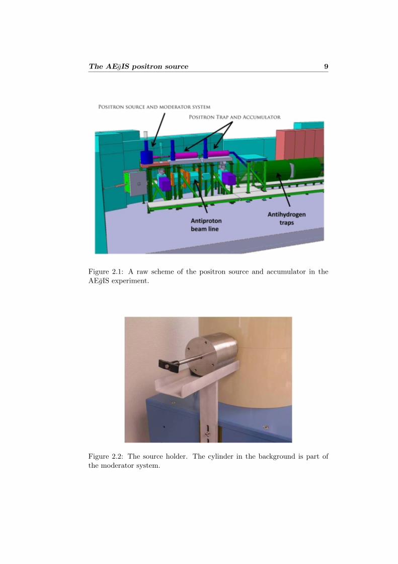
As previously seen, in order to produce Positronium, AEgIS requires anintense monoenergetic positron beam. Thus positrons, emitted from anintense radioactive 22Na source, will be moderated and magnetically guidedto the positron trap and accumulator. Through these last two stages, thebeta plus positron - monoenergetic after the moderation process - are cooled,accumulated and bunched. The operation of the positron trap is based onthe buffer gas slowing down and cooling of positrons in a Penning-Malmbergtrap. A device of this type has been used with success in the ATHENAantimatter experiment [11] and the technology is now so well establishedthat a commercial version of the system is available 1. In this chapter wereport on the first studies about the AEgIS positron source and moderatorsystem that were made during the PhD activity. We will not talk in detailabout the accumulator system (the reader can find more informations in[15]). A scheme of the AEgIS apparatus is shown in figure 2.1.
2.1 The positron source
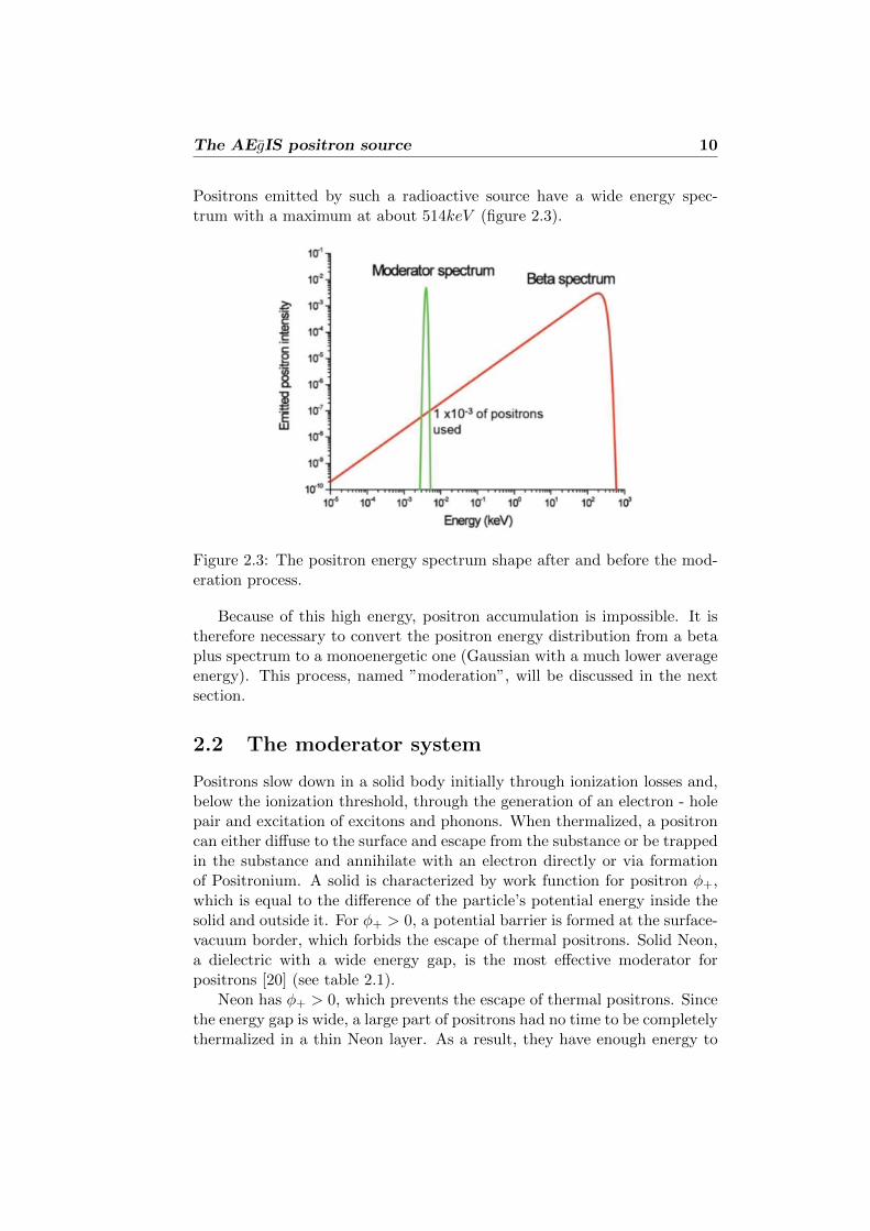
Of all the radionuclides used in experiments as positron sources, the mostconvenient is the 22Na isotope [20]. Its half-life period is 2.6yr, which issufficient for carrying out long-term experiments. The high intensity source(75 mCi) will be supplied by the iThemba Labs and will be located atCERN. This is the most active 22Na radioactive source useful for positronexperiments. For greater activity value the positron emission is reduced byself-absorption. The source was provided with its holder used for insert itsafely into the source plus moderator system as shown in figure 2.2.
In the holder, the 22Na is sealed behind a 13µm tantalum window.
1At the moment, AEgIS has committed a custom-modified positron accumulator tothe First Point Scientific Inc., whose delivery is scheduled for 2011 [19]. Also the sourceand moderator (the commercial name is RGM-2) was ordered in 2010 to the First PointScientific Inc.
8
The AEgIS positron source 9
Figure 2.1: A raw scheme of the positron source and accumulator in theAEgIS experiment.
Figure 2.2: The source holder. The cylinder in the background is part ofthe moderator system.
The AEgIS positron source 10
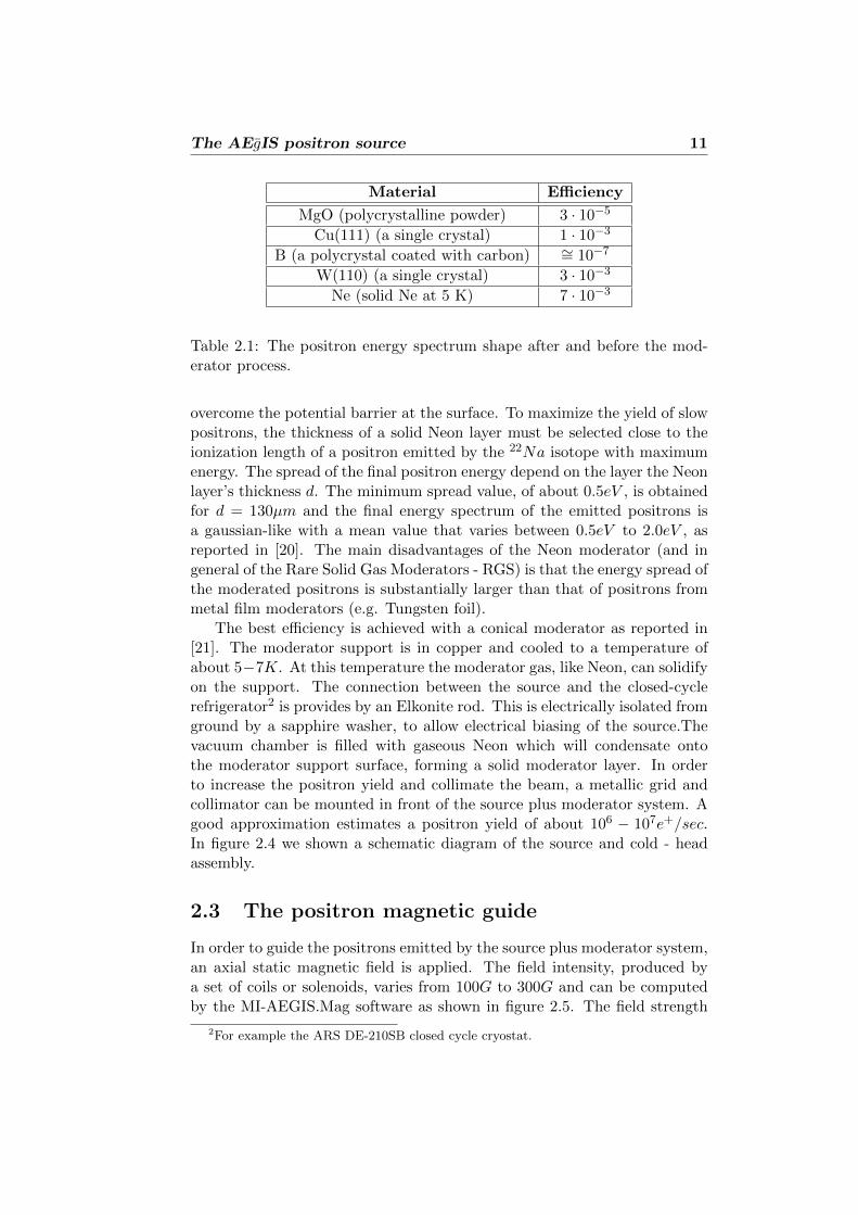
Positrons emitted by such a radioactive source have a wide energy spec-trum with a maximum at about 514keV (figure 2.3).
Figure 2.3: The positron energy spectrum shape after and before the mod-eration process.
Because of this high energy, positron accumulation is impossible. It istherefore necessary to convert the positron energy distribution from a betaplus spectrum to a monoenergetic one (Gaussian with a much lower averageenergy). This process, named ”moderation”, will be discussed in the nextsection.
2.2 The moderator system
Positrons slow down in a solid body initially through ionization losses and,below the ionization threshold, through the generation of an electron - holepair and excitation of excitons and phonons. When thermalized, a positroncan either diffuse to the surface and escape from the substance or be trappedin the substance and annihilate with an electron directly or via formationof Positronium. A solid is characterized by work function for positron φ+,which is equal to the difference of the particle’s potential energy inside thesolid and outside it. For φ+ > 0, a potential barrier is formed at the surface-vacuum border, which forbids the escape of thermal positrons. Solid Neon,a dielectric with a wide energy gap, is the most effective moderator forpositrons [20] (see table 2.1).
Neon has φ+ > 0, which prevents the escape of thermal positrons. Sincethe energy gap is wide, a large part of positrons had no time to be completelythermalized in a thin Neon layer. As a result, they have enough energy to
The AEgIS positron source 11
Material Efficiency
MgO (polycrystalline powder) 3 · 10−5
Cu(111) (a single crystal) 1 · 10−3
B (a polycrystal coated with carbon) ∼= 10−7
W(110) (a single crystal) 3 · 10−3
Ne (solid Ne at 5 K) 7 · 10−3
Table 2.1: The positron energy spectrum shape after and before the mod-erator process.
overcome the potential barrier at the surface. To maximize the yield of slowpositrons, the thickness of a solid Neon layer must be selected close to theionization length of a positron emitted by the 22Na isotope with maximumenergy. The spread of the final positron energy depend on the layer the Neonlayer’s thickness d. The minimum spread value, of about 0.5eV , is obtainedfor d = 130µm and the final energy spectrum of the emitted positrons isa gaussian-like with a mean value that varies between 0.5eV to 2.0eV , asreported in [20]. The main disadvantages of the Neon moderator (and ingeneral of the Rare Solid Gas Moderators - RGS) is that the energy spread ofthe moderated positrons is substantially larger than that of positrons frommetal film moderators (e.g. Tungsten foil).
The best efficiency is achieved with a conical moderator as reported in[21]. The moderator support is in copper and cooled to a temperature ofabout 5−7K. At this temperature the moderator gas, like Neon, can solidifyon the support. The connection between the source and the closed-cyclerefrigerator2 is provides by an Elkonite rod. This is electrically isolated fromground by a sapphire washer, to allow electrical biasing of the source.Thevacuum chamber is filled with gaseous Neon which will condensate ontothe moderator support surface, forming a solid moderator layer. In orderto increase the positron yield and collimate the beam, a metallic grid andcollimator can be mounted in front of the source plus moderator system. Agood approximation estimates a positron yield of about 106 − 107e+/sec.In figure 2.4 we shown a schematic diagram of the source and cold - headassembly.
2.3 The positron magnetic guide
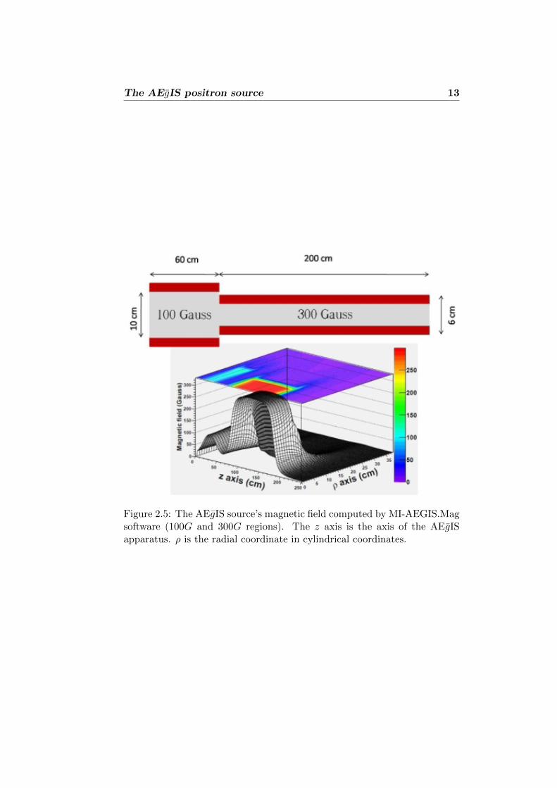
In order to guide the positrons emitted by the source plus moderator system,an axial static magnetic field is applied. The field intensity, produced bya set of coils or solenoids, varies from 100G to 300G and can be computedby the MI-AEGIS.Mag software as shown in figure 2.5. The field strength
2For example the ARS DE-210SB closed cycle cryostat.

The AEgIS positron source 12
Figure 2.4: Schematic diagram of the source and cold-head assembly.
was chosen in order to match the positron trap and accumulator’s inputmagnetic field.
This field’s gradient thus reduce the dimension of the spot by a factor√3 [22]. The positron source produce a forward gamma radiation that can
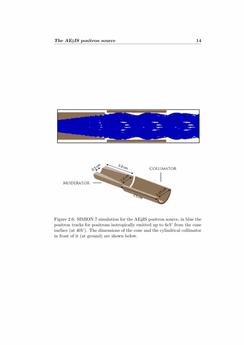
be shielded by inserting an ~E× ~B system in the 300G region. It is possible tosubstitute the ~E× ~B system with a set of curved solenoids or by a magneticslalom system as reported in [20]. However, the ~E × ~B system reduces alsothe energy spread of the positrons. We compute the positron spot radius atthe starting point of the 300G region by developing a SIMION 7.0 simulation.The dimensions of the apparatus and the simulations are shown in figure2.6.
At the end of the positron magnetic guide we expect a radius of about0.66cm comparable with that obtained in a typical positron source appara-tus (i.e. the Surko machine [23]). From the simulations we obtain that thespot dimension does not depend on the positron source potential and nei-ther by the positron energy at the moderator surface (in the range between0.2eV − 2.0eV , in the isotropic emission approximation). The possibility tobuild up a positron source system for AEgIS , supported by references andsimulations, was presented at CERN during the AEgIS meeting, 30th-31stMarch 2009. Respect to a commercial positron source plus moderator sys-tem, the one presented here is more customizable. The main disadvantageis instead the long time need for the R & D of the apparatus.
The AEgIS positron source 13
Figure 2.5: The AEgIS source’s magnetic field computed by MI-AEGIS.Magsoftware (100G and 300G regions). The z axis is the axis of the AEgISapparatus. ρ is the radial coordinate in cylindrical coordinates.
The AEgIS positron source 14
Figure 2.6: SIMION 7 simulation for the AEgIS positron source, in blue thepositron tracks for positrons isotropically emitted up to 6eV from the conesurface (at 40V ). The dimensions of the cone and the cylindrical collimatorin front of it (at ground) are shown below.
The AEgIS positron source 15
2.4 The RGM system
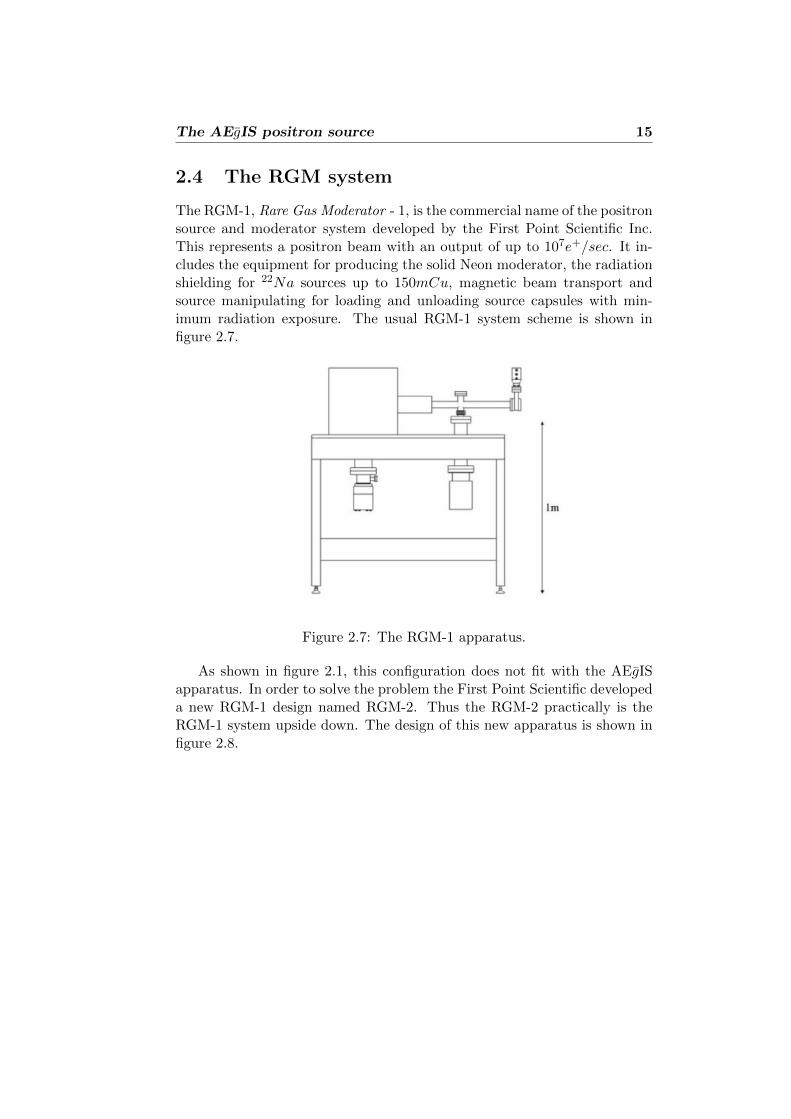
The RGM-1, Rare Gas Moderator - 1, is the commercial name of the positronsource and moderator system developed by the First Point Scientific Inc.This represents a positron beam with an output of up to 107e+/sec. It in-cludes the equipment for producing the solid Neon moderator, the radiationshielding for 22Na sources up to 150mCu, magnetic beam transport andsource manipulating for loading and unloading source capsules with min-imum radiation exposure. The usual RGM-1 system scheme is shown infigure 2.7.
Figure 2.7: The RGM-1 apparatus.
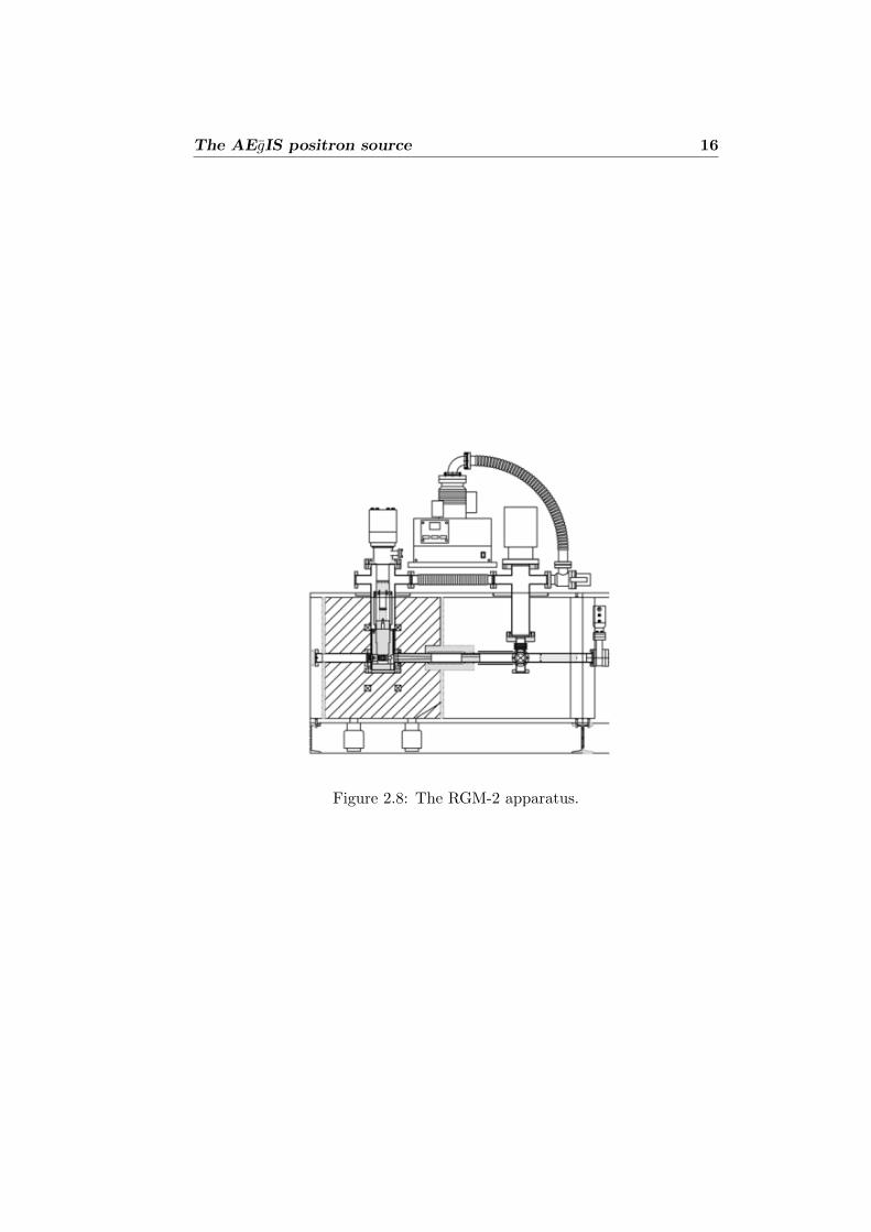
As shown in figure 2.1, this configuration does not fit with the AEgISapparatus. In order to solve the problem the First Point Scientific developeda new RGM-1 design named RGM-2. Thus the RGM-2 practically is theRGM-1 system upside down. The design of this new apparatus is shown infigure 2.8.
The AEgIS positron source 16
Figure 2.8: The RGM-2 apparatus.
Chapter 3
Positronium Physics
3.1 Introduction
The charge exchange reaction between cold antiprotons and Rydberg positro-nium is used in the AEgIS experiment in order to produce cold antihydro-gen, as described in section 1.3.1. Positronium is the simplest quantumelectrodinamical bound system in nature, composed by one electron andone positron [24]. The ground state of positronium, like that of hydrogen,has two possible configurations depending of the relative orientations of thespins of the electron and the positron. The singlet state with antiparal-lel spins is known as para-positronium (pPs) whereas the triplet state withparallel spins is known as ortho-positronium (oPs). In order to conserveC-parity para-positronium and ortho-positronium states should annihilatein different ways with different lifetimes, as expected by quantum electron-dynamics. Para-positronium decay via pPs→ γ + γ and ortho-positroniumoPs→ γ + γ + γ. The lifetime of para-positronium in vacuum was first cal-culated to lowest order of perturbation theory by Wheeler [25]. The morecomplicated calculation of ortho-positronium lifetime in vacuum was done tolowest order of perturbation theory by Ore and Powell [26]. The differencebetween the two lifetimes is due to an additional power of the fine struc-ture constant α which follows directly from the Feynman rules given by theadditional photon in the ortho-positronium annihilation process. Vacuumlifetimes have been calculated to order α7 for para-positronium and order α8
for otho-positronium [27] with results τpPs = 125ps and τoPs = 142ns. Asin the hydrogen atom-case, para-positronium and ortho-positronium atomscan be formed in excited states Ps∗ other than the ground state. Excitedpositronium with high n levels is called Rydberg positronium.
Positronium can not be found in nature. As it is highly unstable the sim-plest way to produce positronium in laboratory is to implant positrons withlow enough kinetic energy into a solid target which is then called converter1.
1It is possible to produce positronium also in liquid and gases as reported in section
17
Positronium Physics 18
Positron slowing down to thermal energies occurs rapidly in comparison withannihilation [28]. Thermal and epithermal positrons can be re-emitted intothe vacuum as positronium atoms after capture of an electron. Almost allpositronium produced are in the ground state2. The positronium forma-tion yield and its energy distribution depend on the nature of the convertermaterial and, for a specific material, on the implantation depth and onthe temperature of the target. In the AEgIS experiment, the ground statepositronium must be excited to n = 20− 30 level by a two step laser pulse[30]. Given that the para-positronium lifetime is too short to allow its laserexcitation before it decays (125ps), in the AEgIS experiment is interestedonly in the fraction of positronium emitted as ortho-positronium (142ns).
3.2 Positronium formation in solids
In this section we will discuss the formation and properties of positroniumin solids. Positronium production occurs in metals and semiconductors aswell as in insulator materials but the production mechanisms are somewhatdifferent.
3.2.1 Positronium formation in metal and semiconductors
In metal and semiconductors, positronium formation is only a surface pro-cess originating from positron back-diffusion or transmission across the sur-face followed by electron capture. Thermalized positrons can produce positro-nium by an adiabatic charge transfer reaction at any converter temperature,provided that the positronium formation potential W is negative:
W = Φ− + Φ+ − 6.8eV < 0 (3.1)
where 6.8eV is the positronium ground state binding energy and Φ− andΦ+ are, respectively, the work functions of the electron and of the positronfor the converter material. In this case, positronium leaves the surface withan energy distribution extending from zero up to the work function energy,resulting in a mean energy of the order of a few eV . If W > 0 the positro-nium adiabatic emission is scarce and mostly due to ephitermal positrons.When also Φ+ < 0 the process of direct positron emission is in competitionwith the adiabatic positronium emission. In addition to the adiabatic emis-sion, thermally activated formation has been observed [31]. This additionalprocess is dominant when the target temperature is of the order of severalhundred kelvin and it is interpreted in terms of surface traps in which thepositrons reside but from which it may be desorbed as positronium. Inthis case positronium has an energy distribution corrisponding to the targettemperature.
3.3.2.2For n = 2 “natural” positronium production see [29].
Positronium Physics 19
3.2.2 Positronium formation in insulators
In insulators, surface formation of positronium by thermal positrons is un-likely since the binding energy of positronium atom is normally insufficient tocompensate for the exctraction of the positron and of the electron (W > 0).However the themalization of positrons in an insulator is less efficient thanin a metal, thus a large flux of positrons returning to the surface of theinsulator with a sufficient kinetic energy to form positronium can be ex-pected. The energy spectrum in this case reflects the energy distribution ofthe ephitermal positrons and may extended up to several eV.
In addition positronium can be formed in the bulk as quasi-positronium3,reach the surface and then be emitted in vacuum. In this case positroniumis formed during the slowing down of positron, mostly when the positronenergy is in the range between Egap−Esolid and Egap (the so called “Ore gap”[33]). Egap is the energy necessary to excite an electron from the valenceto the conduction band and Esolid is the binding energy of the positroniumatom in the solid. In general Esolid < 6.8eV . Bulk positronium formationis also possible when a positron encounters a spur electron, i.e. an electronraised in the conduction band by the positron itself during its slowing down[34]. The positronium atom in solid is a mobile system, as long as it isnot trapped by a defect or self-trapped in a phonon-cloud; it will eventuallyreach the surface with a residual kinetic energy ECM (of the order of few eV )that depends on the depth of formation. The two options described above(surface or bulk formation) depend on the temperature of the converter onlyindirectly, through temperature effects on migration and trapping.
3.2.3 Monte Carlo simulation of Ps formation in solids
Monte Carlo simulation of Ps formation Al2O3
Lacking experimental data, the Monte Carlo simulation of positronium for-mation in solids is the only method that gives informations about the energyspectrum and the angular distribution of the emitted positronium. In orderto achieve this goal, my Master thesis [35] consisted in develop a simulationof positronium formation in insulator materials and in particular in Alumina(Al2O3). The idea is that, when we know precisely the energy and veloc-ity distribution of the emitted positronium atoms, we will implement thepositronium thermalization in nanochannels and/or pores in order to pre-dict the characteristics of the final positronium cloud that will be excited by
3The electron - positron pairs interacting with a solid medium (the so called quasi-positronium) have close analogies with the positronium atom discussed in the introduction,in particular for the spin-dependent part of the wave function, but also it’s possible toexpect important difference in the spatial part of the wave function and in the absolutevalues of the annihilation rates as reported in [32]. However since the second half of ‘90the positronist community decided to use the word positronium also for indicate quasi-positronium atoms. In this PhD thesis we will use this new terminology.
Positronium Physics 20
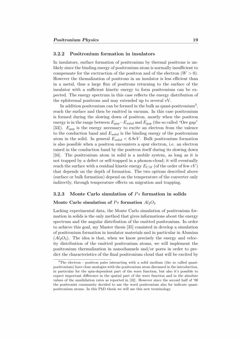
laser. The simulation starts with an ingoing positron with a kinetic energybetween zero and 5keV . Such positron enters in the Alumina solid and itis followed, scattering by scattering, till its energy is grater than the cut-offenergy, fixed in our simulation at 1eV . Two different approach are used forcompute the positron tracks in the range 5keV − 20eV and 20eV − 1eV .If the positron goes back at the solid surface it have a probability PP sto form positronium. This is the first step of an overall simulation of theAEgIS target in which the outgoing positronium hits the inner nanochan-nel surface and lost energy by inelastic scatterings (figure 3.1). Low energypositronium (meV ) is fundamental in order to maximize the antihydrogenproduction cross section for the process Ps∗ + p→ H + e−.
Figure 3.1: The Monte Carlo scheme: in red the positrons slowing down andpositronium formation. In blue the positronium thermalization in orderednanochannels (not considered, at the moment, in our simulations).
The scheme used for the simulation, in the energy range between 5keVand 20eV , is based on the energy loss approximation model [36]. Duringthe slowing down process in matter, the positron undergoes many elasticscattering with the atoms of the media that produce angular deviations ofthe positron path given by the elastic differential cross section. This quan-tity can be computed by solving the Dirac equation for a given electrostatic
Positronium Physics 21
potential in the non-relativistic limit. During the positron slowing down,in addition to elastic scattering we also have inelastic processes, i.e. atomicexcitation, ionization or radiative effects. These processes can be includedusing a “mean” approach studying the positron Energy Stopping Power.This quantity allows us to get the mean energy loss for unity of length. Av-eraging over all inelastic processes involved, it reduces the sensibility of theMonte Carlo to statistical effects that were not considered in our simulation[37]. While the Energy Stopping Power for positrons with energy greaterthan 10keV is theoretically known [38], at energy below 10keV only a fewmodels have been developed. In our simulation, one of these, the H. Gumusmodel [39] was used. However it fails at energy lower than a few tens of eV .At such low energies the inelastic positron interaction depend both on theclass of solids and the solids structure (amorphous or crystalline) or the pres-ence of cavities (without cavities, regular or irregular porous or channeledmedia). In our simulation we considered only amourphous media withoutcavities. This is the case of the Aluminum Oxide Al2O3 (Alumina). This isthe costituent of Whatman R© membrane, that is one of the possible candi-dates for the AEgIS converter. Whatman R© membrane will be discussed insection 3.4.2.
The scheme used in order to simulate the positron tracks in the 20eV −1eV energy range is based on the Ritley scheme [40], originally developedfor solid metals. Each positron with energy less than 20eV is followed tillthe cut-off energy value fixed in our simulation at 1eV . The positron moveson straight lines which length is an appropriate part of the total mean freepath. At the end of every straight line the positron, with a given probabilitydefined by the elastic and inelastic cross sections ratio, makes an elastic orinelastic scattering with a molecule of the medium. In each case the scatteredpositron moves in a new direction and, in the case of inelastic scattering, itloses a quantity ∆E of its kinetic energy.
If the positron backscatters till the surface with kinetic energy in theOre gap, this positron may form positronium with probability PPs that is,in general, a function of the kinetic energy of the inner positron. Giventhat ground state positronium is formed with equal likelihood in the singletstate or in one of the three triplet states, only the 75% of the total amountof positronium formed is ortho-positronium. In our simulation we do notconsider the possibility of positronium formation in the bulk of Aluminaas experimentally found by S. Van Petegem [41]. Neither implement thethermalization of positronium in the Whatman R© membrane nanochannelsor the positronium formation in the space between alumina grains. The sim-ulated positronium energy spectrum and angular distribution for Aluminaare shown in figure 3.2.

Positronium Physics 22
Figure 3.2: Positronium energy spectrum and angular distribution forpositrons implanted in Alumina (Al2O3). Angles are referred to the positroningoing direction. The 18eV cut-off in energy is due to the the maximumpositronium energy permetted by the Ore gap model.
Positronium Physics 23
Extension to amorphous SiO2 and limits of Monte Carlo simula-tions
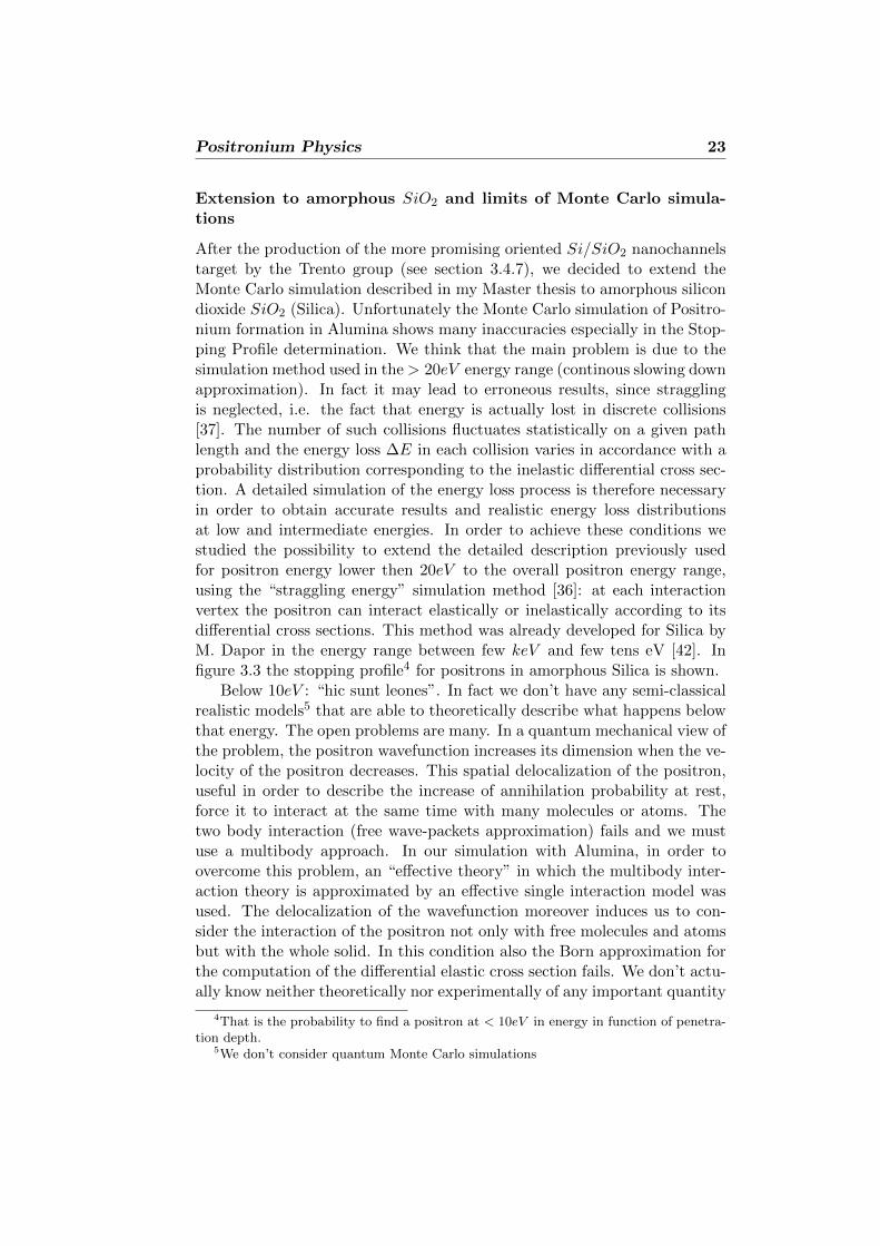
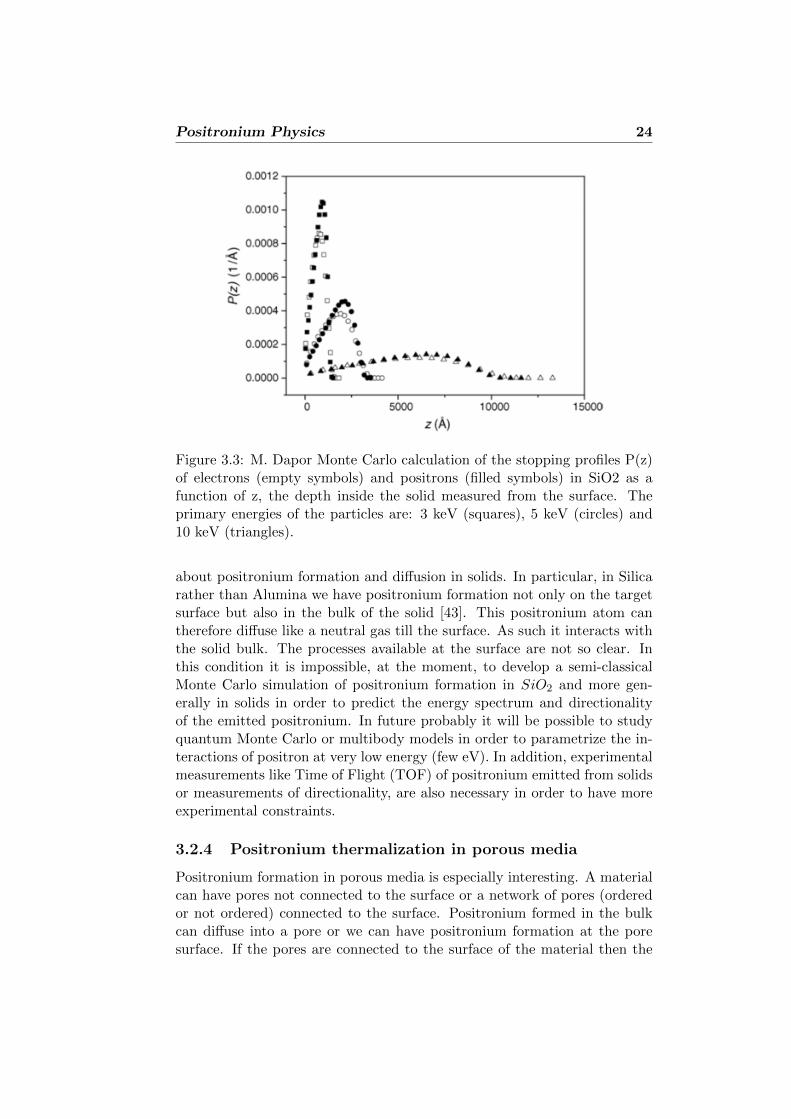
After the production of the more promising oriented Si/SiO2 nanochannelstarget by the Trento group (see section 3.4.7), we decided to extend theMonte Carlo simulation described in my Master thesis to amorphous silicondioxide SiO2 (Silica). Unfortunately the Monte Carlo simulation of Positro-nium formation in Alumina shows many inaccuracies especially in the Stop-ping Profile determination. We think that the main problem is due to thesimulation method used in the> 20eV energy range (continous slowing downapproximation). In fact it may lead to erroneous results, since stragglingis neglected, i.e. the fact that energy is actually lost in discrete collisions[37]. The number of such collisions fluctuates statistically on a given pathlength and the energy loss ∆E in each collision varies in accordance with aprobability distribution corresponding to the inelastic differential cross sec-tion. A detailed simulation of the energy loss process is therefore necessaryin order to obtain accurate results and realistic energy loss distributionsat low and intermediate energies. In order to achieve these conditions westudied the possibility to extend the detailed description previously usedfor positron energy lower then 20eV to the overall positron energy range,using the “straggling energy” simulation method [36]: at each interactionvertex the positron can interact elastically or inelastically according to itsdifferential cross sections. This method was already developed for Silica byM. Dapor in the energy range between few keV and few tens eV [42]. Infigure 3.3 the stopping profile4 for positrons in amorphous Silica is shown.
Below 10eV : “hic sunt leones”. In fact we don’t have any semi-classicalrealistic models5 that are able to theoretically describe what happens belowthat energy. The open problems are many. In a quantum mechanical view ofthe problem, the positron wavefunction increases its dimension when the ve-locity of the positron decreases. This spatial delocalization of the positron,useful in order to describe the increase of annihilation probability at rest,force it to interact at the same time with many molecules or atoms. Thetwo body interaction (free wave-packets approximation) fails and we mustuse a multibody approach. In our simulation with Alumina, in order toovercome this problem, an “effective theory” in which the multibody inter-action theory is approximated by an effective single interaction model wasused. The delocalization of the wavefunction moreover induces us to con-sider the interaction of the positron not only with free molecules and atomsbut with the whole solid. In this condition also the Born approximation forthe computation of the differential elastic cross section fails. We don’t actu-ally know neither theoretically nor experimentally of any important quantity
4That is the probability to find a positron at < 10eV in energy in function of penetra-tion depth.
5We don’t consider quantum Monte Carlo simulations
Positronium Physics 24
Figure 3.3: M. Dapor Monte Carlo calculation of the stopping profiles P(z)of electrons (empty symbols) and positrons (filled symbols) in SiO2 as afunction of z, the depth inside the solid measured from the surface. Theprimary energies of the particles are: 3 keV (squares), 5 keV (circles) and10 keV (triangles).
about positronium formation and diffusion in solids. In particular, in Silicarather than Alumina we have positronium formation not only on the targetsurface but also in the bulk of the solid [43]. This positronium atom cantherefore diffuse like a neutral gas till the surface. As such it interacts withthe solid bulk. The processes available at the surface are not so clear. Inthis condition it is impossible, at the moment, to develop a semi-classicalMonte Carlo simulation of positronium formation in SiO2 and more gen-erally in solids in order to predict the energy spectrum and directionalityof the emitted positronium. In future probably it will be possible to studyquantum Monte Carlo or multibody models in order to parametrize the in-teractions of positron at very low energy (few eV). In addition, experimentalmeasurements like Time of Flight (TOF) of positronium emitted from solidsor measurements of directionality, are also necessary in order to have moreexperimental constraints.
3.2.4 Positronium thermalization in porous media
Positronium formation in porous media is especially interesting. A materialcan have pores not connected to the surface or a network of pores (orderedor not ordered) connected to the surface. Positronium formed in the bulkcan diffuse into a pore or we can have positronium formation at the poresurface. If the pores are connected to the surface of the material then the
Positronium Physics 25
positronium can escape toward the vacuum following the pore channels andcolliding with the pore walls. The energy spectrum of the emitted positro-nium depends on the energy of the positronium entering the pore, on thenumber of collisions with a pore surface and on the mean energy loss foreach collision. Trough this processes it is possible to reduce the positroniumenergy from a few eV to a few meV [44]. This is one of the two requirementsof the AEgIS laser excitation system: few meV positronium atoms in a smalldimension cloud (of the order of few millimeters). As seen previously, we areinterested only in the fraction of positronium emitted as ortho-positronium.Annihilation of the ortho-positronium by pick-off [45] with the pore wallscan not be avoided but the total pick-off loss is expected to remain at thetolerable level of 60%-70%. Moreover has given that the depth in the bulkwhere positronium is formed depends on the positron energy, with an ap-propriate design of the pore geometry and by controlling the implantationdepth through the positron implantation energy, we will be able to tailor theenergy spectrum of the emitted positronium to match the required valuesand possibly give directionality at the positronium cloud in order to increasethe solid angle efficiency for the laser excitation. Some of this aspects, sup-ported by experimental results obtained by the collaboration, will be treatedin the next sections.
3.3 Positronium detection
The understanding of the directionality of the emitted ortho-positronium,its energy spectrum and its yield are the main goals of the AEgIS converterR&D. The first two requests need Time Of Flight measurements (TOF)that, up to now, are only partially available6. The measurements of positro-nium formation yield were performed by means of a monoenergetic positronbeam7 using the well-known “3γ method” described in subsection 3.3.3.Theamount of positronium emitted in vacuum depends on the pick-off annihi-lation reduction that is the size of pores or channels. This quantity canbe experimentally obtained by Positron Annihilation Lifetime Spectroscopymeasurements as described in subsection 3.3.1.
3.3.1 Positron Annihilation Lifetime Spectroscopy
PALS (Positron Annihilation Lifetime Spectroscopy) is a technique thatallows to analyse the microscopic structure of a given material by ortho-positronium lifetime measurements. When a positron interacts with matterit can undergo a free annihilation e+ + e− → γ + γ or form positronium invoids or in the bulk of the solid [31] e+ +e− → Ps. If the ortho-positronium
6Some TOF measurements are achieved at Trento laboratory by R. Brusa et al.7L-NESS laboratory in Como. For more information http://lness.como.polimi.it
Positronium Physics 26
can not escape from the solid, it is subject to pick-off effects. This effect is thedetection of premature annihilations when positrons are ”picked off” by freeelectrons from an enclosing surface. Suppose that two positronium atomsare trapped in an arbitrary material, one in a large hole (or pore) and one inin a small pore. As the positronium atoms move in their pores, the positronwithin the atom has a chance to pick off electrons from the material, causinga premature annihilation. The likelihood of the pick-off effect is determinedby the characteristics of the pore, so the atom in the small pore shouldhave, on average, a shorter lifetime than the one in the large pore. Fromthe lifetime data, you can infer information about the surroundings of theatom. Most part of the positron annihilation take place in two gamma withenergy 511keV by free annihilation e+ + e− → γ + γ, by para-positroniumdecay pPs→ γ+γ and by pickoff ortho-positronium oPs+e− → γ+γ+e−.This two annihilation gamma are emitted in opposite directions in order toconserve energy and momentum. In addition, if the positron is produced bya Sodium-22 radioactive decay there is a 1280keV gamma associated to thepositron emission. Therefore, we can compute the positron or positroniumlifetime in the solid as the delay time between the 1280keV (start) and a511keV (stop) gamma detection. In this procedure we neglect the timebetween the emission of a positron and the 1280keV gamma (about 2−3ps)and the time between the emission of a positron and its implantation inthe solid (about 20− 30ps). If the solids have sets of pores with about thesame dimensions the overall positron annihilation lifetime is a weighted sumof lifetimes given by free, para-positronium and pick-off ortho-positroniumannihilations. If we don’t have losses of positronium atoms in void theweight of lifetime components is the amount of positronium formation inthe sample. Vice versa if we measure the positron lifetime components weobtain information about the pore dimensions using for example the Tao-Eldrup model [46]. PALS is therefore an important tool in order to measurethe dimensions of converter voids like nano-channels or pores. Given that theAEgIS converters emit a lot of positronium in vacuum we can’t use PALS forpositronium yield measurements. During my PhD activity I studied also thepositronium formation in Pseudocumene with PALS technique, as reportedin the following.
PALS apparatus in the Milano Politecnico Positron Laboratory
Positrons are generally obtained from 22Na, a radioisotope which also emitsa prompt γ-ray with an energy of 1280keV . This start signal marks the birthof the positron. The stop signal is given by one of the annihilation photons(0.511 MeV): most of the annihilations occur into two gamma rays. Thesource strength is typically 0.04 to 0.8 MBq, and the source is prepared bydepositing a droplet of an aqueous solution containing 22Na on a thin metal-lic foil or plastic sheet; after drying the residue is subsequently covered by an
Positronium Physics 27
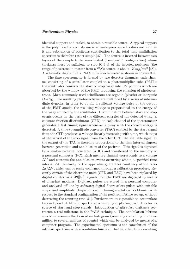
identical support and sealed, to obtain a reusable source. A typical supportis the polymide Kapton; its use is advantageous since Ps does not form init and subtraction of positrons contribution to the total time annihilationspectrum is therefore rather simple [47]. The source is inserted between twolayers of the sample to be investigated (”sandwich” configuration) whosethickness must be sufficient to stop 99.9 % of the injected positrons (therange of positrons in matter from a 22Na source is about 170mg/cm2 [48]).A schematic diagram of a PALS time spectrometer is shown in Figure 3.4.
The time spectrometer is formed by two detector channels: each chan-nel consisting of a scintillator coupled to a photomultiplier tube (PMT);the scintillator converts the start or stop γ-ray into UV photons which areabsorbed by the window of the PMT producing the emission of photoelec-trons. Most commonly used scintillators are organic (plastic) or inorganic(BaF2). The resulting photoelectrons are multiplied by a series of interme-diate dynodes, in order to obtain a sufficient voltage pulse at the outputof the PMT anode; the resulting voltage is proportional to the energy ofthe γ-ray emitted by the scintillator. Discrimination between start and stopevents occurs on the basis of the different energies of the detected γ-ray: aconstant fraction discriminator (CFD) on each channel of the spectrometergenerates a fast timing signal whenever a γ-ray with the correct energy isdetected. A time-to-amplitude converter (TAC) enabled by the start signalfrom the CFD produces a voltage linearly increasing with time, which stopsat the arrival of the stop signal from the other CFD: the available signal atthe output of the TAC is therefore proportional to the time interval elapsedbetween generation and annihilation of the positron. This signal is digitizedby a analog-to-digital converter (ADC) and transferred to the memory ofa personal computer (PC). Each memory channel corresponds to a voltage∆V and contains the annihilation events occurring within a specified timeinterval ∆t. Linearity of the apparatus guarantees constancy of the ratio∆t/∆V , which can be easily confirmed through a calibration procedure. Re-cently certain of the electronic units (CFD and TAC) have been replaced bydigital counterparts [49][50]: signals from the PMT are digitized by meansof ultra-fast modules. Digitized pulses are stored in a personal computerand analysed off-line by software; digital filters select pulses with suitableshape and amplitude. Improvement in timing resolution is obtained withrespect to the standard configuration of the positron lifetime set-up, withoutdecreasing the counting rate [51]. Furthermore, it is possible to accumulatetwo independent lifetime spectra at a time, by exploiting each detector assource of start and stop signals. Introduction of ultra-fast digitizers rep-resents a real milestone in the PALS technique. The annihilation lifetimespectrum assumes the form of an histogram (generally containing from onemillion to several millions of counts) which can be analyzed by means of acomputer program. The experimental spectrum is the convolution of theintrinsic spectrum with a resolution function, that is, a function describing
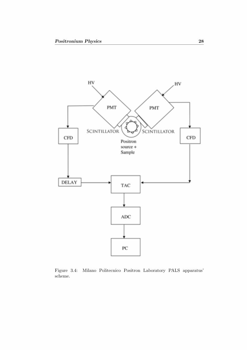
Positronium Physics 28
Figure 3.4: Milano Politecnico Positron Laboratory PALS apparatus’scheme.
Positronium Physics 29
the response of the apparatus to two simultaneous events. This can be ob-tained [48] from the time spectrum of 60Co, which decays by emitting twogamma rays with similar energies (1.33 and 1.17 MeV) within a time inter-val of about 0.7 ps. The two events can be considered simultaneous on thetypical time scale of PALS and the corresponding time spectrum is oftenassumed to represent the resolution function of the positron annihilationlifetime spectrum, although the energy of the annihilation photon is ratherdifferent with respect to the 60Co gamma rays. In fact, the full width at halfmaximum (FWHM) for a time spectrum with 1.274 and 0.511 MeV gammasis larger (by a factor of about 1.1) than that for 1.17 and 1.33 MeV gammas.A better approach is to use the time spectrum of 207Bi, which decays to anexcited state of 207Pb with half life of 30 years. In the de-excitation processof 207Pb to the ground state two gammas, with respective energies of 1.06and 0.57 MeV, are emitted, with a lifetime of 182 ps. The energies of the twophotons are very near to those corresponding to the start and stop photonsin PALS. Deconvolution of the 207Bi time spectrum with a single fixed life-time provides a realistic resolution function, which may be represented by asingle gaussian or a sum of gaussians with different centroids and weights;values between 150 and 300 ps are quite common for the FWHM of theresolution function. Various computer codes are available [52][53][54] [55] toanalyse the annihilation lifetime spectrum in terms of different components,each corresponding to a particular positron state. A PALS spectrum con-sists thus of the sum of a number of components, which can be treated asdiscrete or and continuous. In the first case, each annihilation component isan exponential function of the form I
τ e− tτ , each characterized by a lifetime
τ and an intensity I. The intrinsic spectrum S(t) can be written:
S(t) = R(t)⊗
[N∑i=1
Iiτie− tτi +B
](3.2)
where R(t) is the resolution function and B is the constant background, rep-resenting the spurious coincidence events, to be subtracted during the fittingprocedure. The symbol ⊗ stands for the convolution operation. PALS anal-yses in terms of three components (that is, N = 3) are quite common.Typical lifetimes of free positrons (i.e., those that do not form Ps) in poly-mers are around 0.4 ns. p-Ps lifetimes in condensed matter are usually below0.15 ns; o-Ps shows the longest lifetimes, generally in the range 1-10 ns. Acontinuous PALS spectral component is constructed as a continuous sum ofdiscrete components and is characterized by three parameters: the inten-sity and the first two moments of the distribution of lifetimes, that is, thecentroid (mean lifetime) and second moment (standard deviation from themean lifetime). A distribution of o-Ps lifetimes is expected in a polymericmaterial, and will depend on the hole volume distribution present in theamorphous zones. Both the computer programs MELT [54] and CONTIN
Positronium Physics 30
[53] analyse the time annihilation spectrum only in terms of continuous com-ponents, without any guess as to the shape of the distributions. Conversely,the code POSITRONFIT [52] provides analyses only in term of discretecomponents. The program LT [55] is also able to provide for eventual dis-tributions of lifetimes (assuming a log-normal distribution) and can be usedfor a mixed analysis, in the sense that each component can be chosen tobe discrete or continuous. Of course, the statistics of a spectrum must besubstantially higher than as in the case of discrete component, if continuouscomponents are to be accurately resolved.
As an application of these techniques we present a study of the effectsof the otrhopositronium formation in organic liquid scintillators on electronanti-neutrino detection. This study was made as a part of my PhD program.
3.3.2 Technical application: effects of the oPs formation inorganic liquid scintillators on electron anti-neutrinodetection
Electron anti-neutrinos are produced in β decays of naturally occurring ra-dioactive isotopes in the Earth, representing a unique direct probe of ourplanet’s interior. Also nuclear reactors provide intense sources of antineu-trinos, which come from the decay of neutron-rich fragments produced byheavy element fissions. Electron anti-neutrinos are often detected with thereaction:
νe + p→ n+ e+ (3.3)
by looking at the neutron-positron coincidence.Organic liquid scintillators:
• Neutrons are captured mainly on protons, and identified looking atthe characteristic 2.23MeV gamma ray emitted in the reaction:
n+ p→ d+ γ (3.4)
The neutron mean capture time varies from few up to hundreds mi-croseconds.
• Positrons interacting in liquid scintillator may either annihilate withelectrons or form positronium (Ps). In condensed matter, however, in-teractions of otho-positronium with the surrounding medium stronglyreduce its lifetime: processes like chemical reactions, spin-flip (ortho-para conversion at paramagnetic centers), or pick-off annihilation oncollision with an anti-parallel spin electron, lead to the two body de-cay with lifetimes of a few nanoseconds. The surviving three bodydecay channel oPs → γ + γ + γ is typically reduced to a negligiblefraction (ortho-positronium can not excape in vacuum). If the de-lay introduced by the positron annihilation lifetime is of the order of a
Positronium Physics 31
few nanoseconds, calorimetric scintillation detectors, like Borexino [56]and KamLAND [57], are unable to disentangle the energy deposited bypositron interactions from that released by annihilation gamma rays.In these cases, a delayed gamma ray emission induces a distortion inthe time distribution of emitted scintillation photons (pulse shape),with respect to a pure annihilation event. Such distortion can affectalgorithms based on the pulse shape, like the position reconstructionand the particle discrimination. As second order effect, positron en-ergy reconstruction can be distorted if a correction based on the energydependency on position is applied.
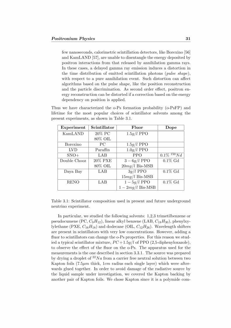
Thus we have characterized the o-Ps formation probability (o-PsFP) andlifetime for the most popular choices of scintillator solvents among thepresent experiments, as shown in Table 3.1.
Experiment Scintillator Fluor Dope
KamLAND 20% PC 1.5g/l PPO80% OIL
Borexino PC 1.5g/l PPO
LVD Paraffin 1.0g/l PPO
SNO+ LAB PPO 0.1% 150Nd
Double Chooz 20% PXE 3− 6g/l PPO 0.1% Gd80% OIL 20mg/l Bis-MSB
Daya Bay LAB 3g/l PPO 0.1% Gd15mg/l Bis-MSB
RENO LAB 1− 5g/l PPO 0.1% Gd1− 2mg/l Bis-MSB
Table 3.1: Scintillator composition used in present and future undergroundneutrino experiment.
In particular, we studied the following solvents: 1,2,3 trimetilbenzene orpseudocumene (PC, C9H12), linear alkyl benzene (LAB, C18H30), phenylxy-lylethane (PXE, C16H18) and dodecane (OIL, C12H26). Wavelength shiftersare present in scintillators with very low concentrations. However, adding afluor to scintillators can change the o-Ps properties. For this reason we stud-ied a typical scintillator mixture, PC+1.5g/l of PPO (2,5-diphenyloxazole),to observe the effect of the fluor on the o-Ps. The apparatus used for themeasurements is the one described in section 3.3.1. The source was preparedby drying a droplet of 22Na from a carrier free neutral solution between twoKapton foils (7.5µm thick, 1cm radius each single layer) which were after-wards glued together. In order to avoid damage of the radiative source bythe liquid sample under investigation, we covered the Kapton backing byanother pair of Kapton foils. We chose Kapton since it is a polymide com-
Positronium Physics 32
patible with scintillator materials and where positrons do not form Ps. Thesource has an activity of 0.8 MBq. The Kapton-source sandwich is pouredin a glass vial, containing the scintillator sample. The vial is positionedbetween the two plastic scintillator detectors.
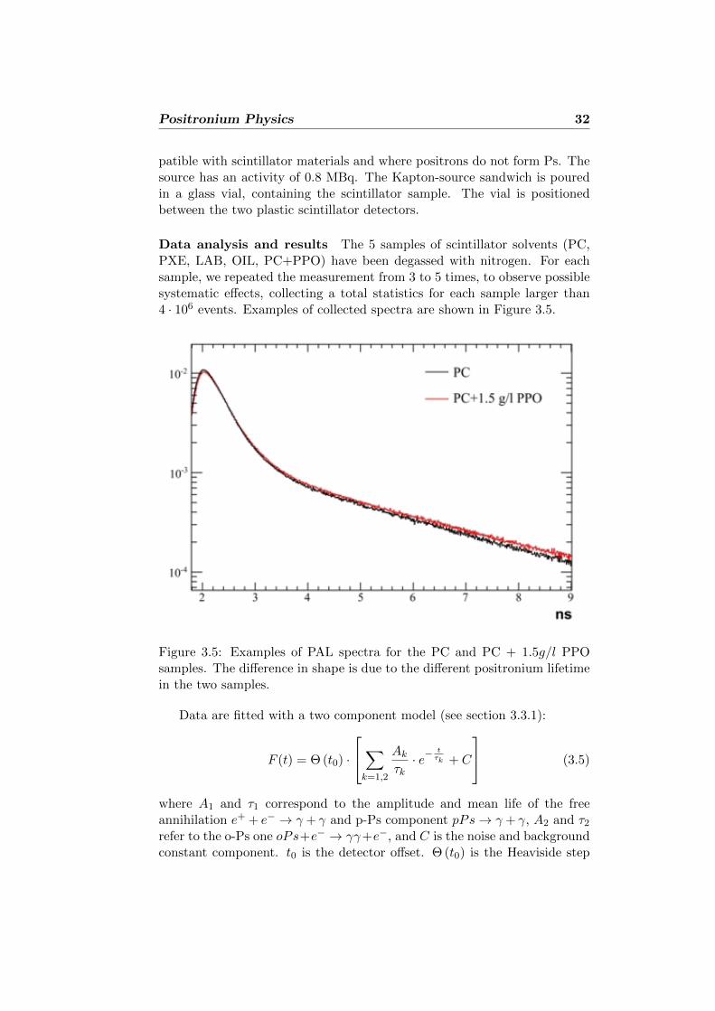
Data analysis and results The 5 samples of scintillator solvents (PC,PXE, LAB, OIL, PC+PPO) have been degassed with nitrogen. For eachsample, we repeated the measurement from 3 to 5 times, to observe possiblesystematic effects, collecting a total statistics for each sample larger than4 · 106 events. Examples of collected spectra are shown in Figure 3.5.
Figure 3.5: Examples of PAL spectra for the PC and PC + 1.5g/l PPOsamples. The difference in shape is due to the different positronium lifetimein the two samples.
Data are fitted with a two component model (see section 3.3.1):
F (t) = Θ (t0) ·
∑k=1,2
Akτk· e−
tτk + C
(3.5)
where A1 and τ1 correspond to the amplitude and mean life of the freeannihilation e+ + e− → γ + γ and p-Ps component pPs→ γ + γ, A2 and τ2
refer to the o-Ps one oPs+e− → γγ+e−, and C is the noise and backgroundconstant component. t0 is the detector offset. Θ (t0) is the Heaviside step

Positronium Physics 33
function in t0. The fit function F (t) is convoluted with the resolution of theapparatus, modelled with the sum of two gaussians:
G(t) =∑i=1,2
gi√2πσ2
i
· e− t2
2σ2i (3.6)
centred in the same value but with different resolutions (σ1 and σ2), andwhere g1 + g2 = 1. The detector resolution is dominated by the first com-ponent with σ1
∼= 110ps (g1∼= 0.8), while σ2
∼= 160ps. The data modelingpackage used in this analysis is the RooFit toolkit, embedded in the ROOTpackage, based on MINUIT [58]. All the parameters in the model are freein the fit, and all the fits to the data samples produced a normalized χ2
in the 0.85 − 0.98 range. The parameter τ1 is almost constant in all themeasurements: the mean value is centered around 365ps, with a root meansquare of 8ps. An example of fit for the PXE sample is shown in Figure 3.6.
Figure 3.6: Fit (red line) of the positron annihilation life time spectrum(black dots) for the PXE sample.
We made an attempt to add an exponential component to the model, todisentangle free annihilation from p-Ps, but the fit was not able to determinethe minimum. To estimate the fraction of positrons annihilating in Kapton,we covered the 22Na source with 1 to 3 Kapton layers. The Kapton-sourcesandwiches were inserted in a Plexiglas medium, characterized by an o-Psmean life of ∼= 2ns and the atomic number Z compatible to the scintillators’
Positronium Physics 34
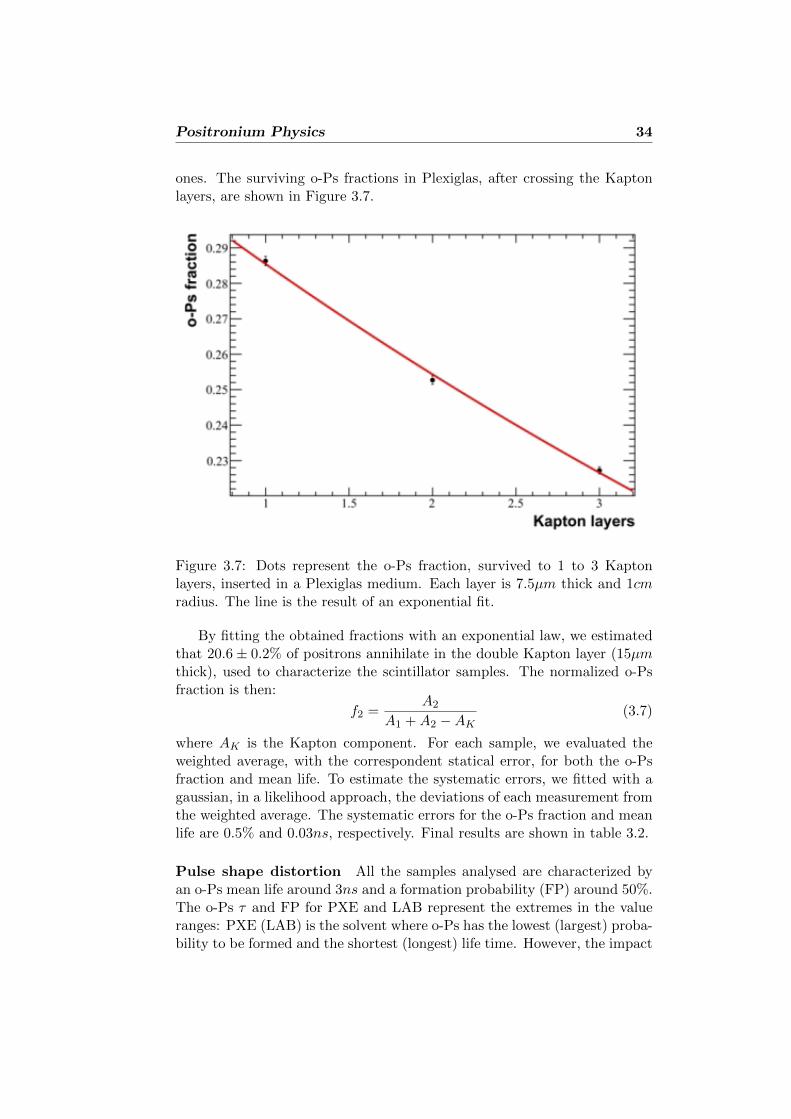
ones. The surviving o-Ps fractions in Plexiglas, after crossing the Kaptonlayers, are shown in Figure 3.7.
Figure 3.7: Dots represent the o-Ps fraction, survived to 1 to 3 Kaptonlayers, inserted in a Plexiglas medium. Each layer is 7.5µm thick and 1cmradius. The line is the result of an exponential fit.
By fitting the obtained fractions with an exponential law, we estimatedthat 20.6± 0.2% of positrons annihilate in the double Kapton layer (15µmthick), used to characterize the scintillator samples. The normalized o-Psfraction is then:
f2 =A2
A1 +A2 −AK(3.7)
where AK is the Kapton component. For each sample, we evaluated theweighted average, with the correspondent statical error, for both the o-Psfraction and mean life. To estimate the systematic errors, we fitted with agaussian, in a likelihood approach, the deviations of each measurement fromthe weighted average. The systematic errors for the o-Ps fraction and meanlife are 0.5% and 0.03ns, respectively. Final results are shown in table 3.2.
Pulse shape distortion All the samples analysed are characterized byan o-Ps mean life around 3ns and a formation probability (FP) around 50%.The o-Ps τ and FP for PXE and LAB represent the extremes in the valueranges: PXE (LAB) is the solvent where o-Ps has the lowest (largest) proba-bility to be formed and the shortest (longest) life time. However, the impact
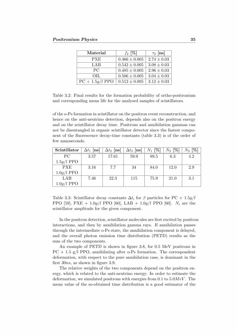
Positronium Physics 35
Material f2 [%] τ2 [ns]
PXE 0.466± 0.005 2.74± 0.03
LAB 0.542± 0.005 3.08± 0.03
PC 0.485± 0.005 2.96± 0.03
OIL 0.506± 0.005 3.04± 0.03
PC + 1.5g/l PPO 0.512± 0.005 3.12± 0.03
Table 3.2: Final results for the formation probability of ortho-positroniumand corresponding mean life for the analysed samples of scintillators.
of the o-Ps formation in scintillator on the positron event reconstruction, andhence on the anti-neutrino detection, depends also on the positron energyand on the scintillator decay time. Positrons and annihilation gammas cannot be disentangled in organic scintillator detector since the fastest compo-nent of the fluorescence decay-time constants (table 3.3) is of the order offew nanoseconds.
Scintillator ∆t1 [ns] ∆t2 [ns] ∆t3 [ns] N1 [%] N2 [%] N3 [%]
PC 3.57 17.61 59.9 89.5 6.3 4.21.5g/l PPO
PXE 3.16 7.7 34 84.0 12.0 2.91.0g/l PPO
LAB 7.46 22.3 115 75.9 21.0 3.11.0g/l PPO
Table 3.3: Scintillator decay constants ∆ti for β particles for PC + 1.5g/lPPO [59], PXE + 1.0g/l PPO [60], LAB + 1.0g/l PPO [60]. Ni are thescintillator amplitude for the given component.
In the positron detection, scintillator molecules are first excited by positroninteractions, and then by annihilation gamma rays. If annihilation passesthrough the intermediate o-Ps state, the annihilation component is delayed,and the overall photon emission time distribution (PETD) results as thesum of the two components.
An example of PETD is shown in figure 3.8, for 0.5 MeV positrons inPC + 1.5 g/l PPO, annihilating after o-Ps formation. The correspondentdeformation, with respect to the pure annihilation case, is dominant in thefirst 30ns, as shown in figure 3.9.
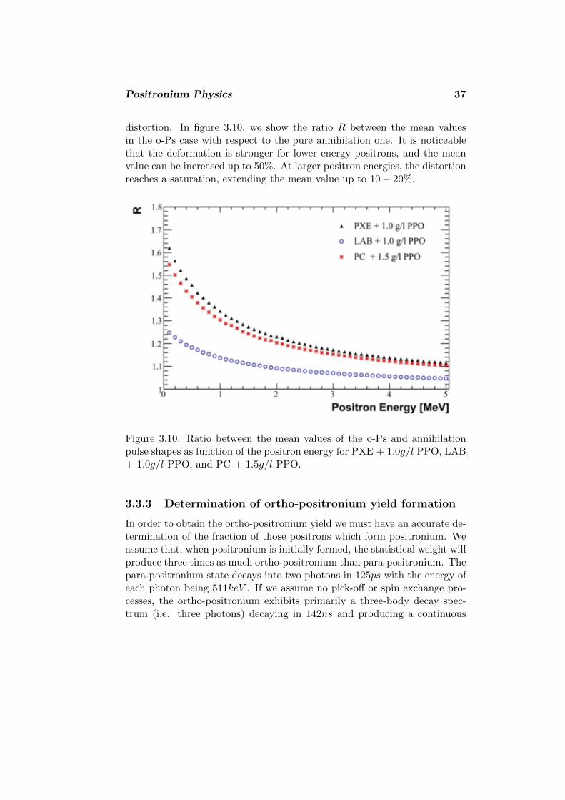
The relative weights of the two components depend on the positron en-ergy, which is related to the anti-neutrino energy. In order to estimate thedeformation, we simulated positrons with energies from 0.1 to 5.0MeV . Themean value of the so-obtained time distribution is a good estimator of the
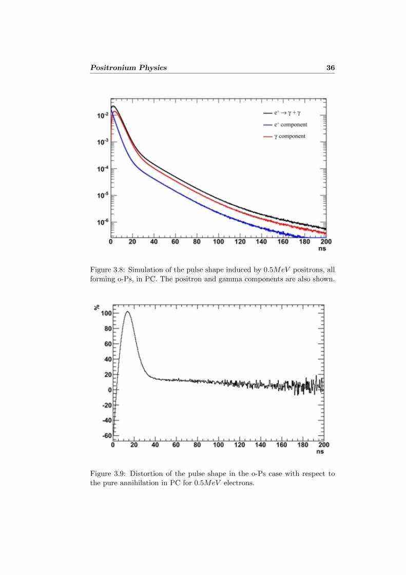
Positronium Physics 36
Figure 3.8: Simulation of the pulse shape induced by 0.5MeV positrons, allforming o-Ps, in PC. The positron and gamma components are also shown.
Figure 3.9: Distortion of the pulse shape in the o-Ps case with respect tothe pure annihilation in PC for 0.5MeV electrons.
Positronium Physics 37
distortion. In figure 3.10, we show the ratio R between the mean valuesin the o-Ps case with respect to the pure annihilation one. It is noticeablethat the deformation is stronger for lower energy positrons, and the meanvalue can be increased up to 50%. At larger positron energies, the distortionreaches a saturation, extending the mean value up to 10− 20%.
Figure 3.10: Ratio between the mean values of the o-Ps and annihilationpulse shapes as function of the positron energy for PXE + 1.0g/l PPO, LAB+ 1.0g/l PPO, and PC + 1.5g/l PPO.
3.3.3 Determination of ortho-positronium yield formation
In order to obtain the ortho-positronium yield we must have an accurate de-termination of the fraction of those positrons which form positronium. Weassume that, when positronium is initially formed, the statistical weight willproduce three times as much ortho-positronium than para-positronium. Thepara-positronium state decays into two photons in 125ps with the energy ofeach photon being 511keV . If we assume no pick-off or spin exchange pro-cesses, the ortho-positronium exhibits primarily a three-body decay spec-trum (i.e. three photons) decaying in 142ns and producing a continuous
Positronium Physics 38
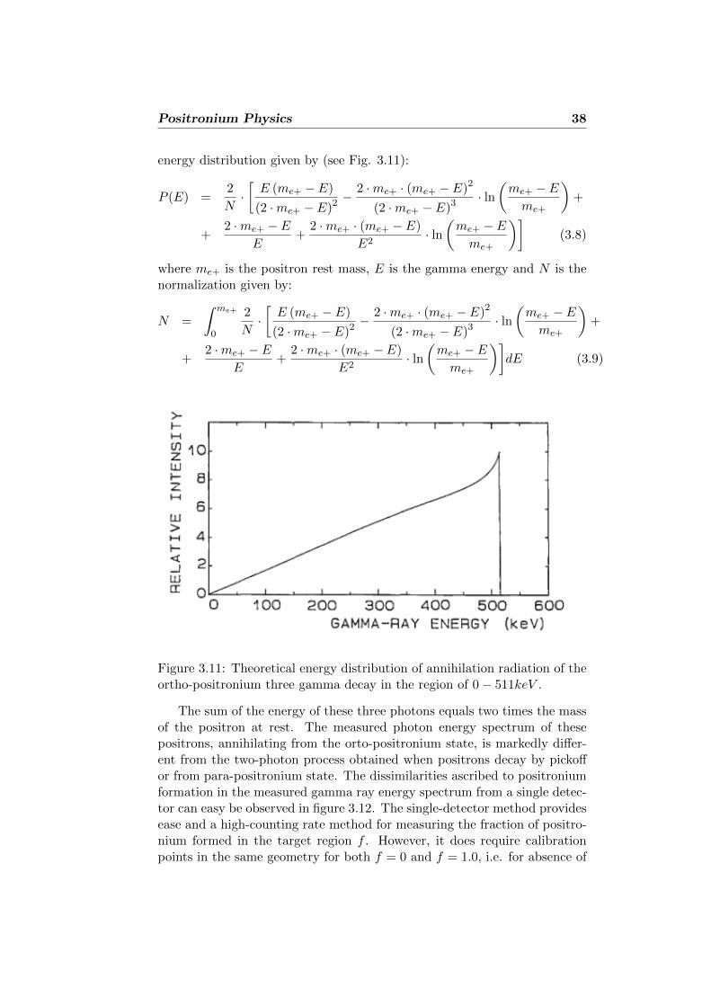
energy distribution given by (see Fig. 3.11):
P (E) =2
N·[E (me+ − E)
(2 ·me+ − E)2 −2 ·me+ · (me+ − E)2
(2 ·me+ − E)3 · ln(me+ − Eme+
)+
+2 ·me+ − E
E+
2 ·me+ · (me+ − E)
E2· ln(me+ − Eme+
)](3.8)
where me+ is the positron rest mass, E is the gamma energy and N is thenormalization given by:
N =
∫ me+
0
2
N·[E (me+ − E)
(2 ·me+ − E)2 −2 ·me+ · (me+ − E)2
(2 ·me+ − E)3 · ln(me+ − Eme+
)+
+2 ·me+ − E
E+
2 ·me+ · (me+ − E)
E2· ln(me+ − Eme+
)]dE (3.9)
Figure 3.11: Theoretical energy distribution of annihilation radiation of theortho-positronium three gamma decay in the region of 0− 511keV .
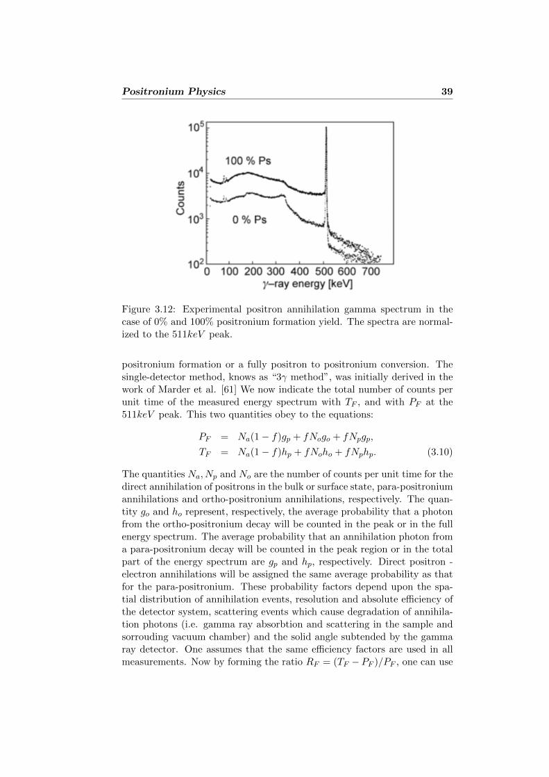
The sum of the energy of these three photons equals two times the massof the positron at rest. The measured photon energy spectrum of thesepositrons, annihilating from the orto-positronium state, is markedly differ-ent from the two-photon process obtained when positrons decay by pickoffor from para-positronium state. The dissimilarities ascribed to positroniumformation in the measured gamma ray energy spectrum from a single detec-tor can easy be observed in figure 3.12. The single-detector method providesease and a high-counting rate method for measuring the fraction of positro-nium formed in the target region f . However, it does require calibrationpoints in the same geometry for both f = 0 and f = 1.0, i.e. for absence of
Positronium Physics 39
Figure 3.12: Experimental positron annihilation gamma spectrum in thecase of 0% and 100% positronium formation yield. The spectra are normal-ized to the 511keV peak.
positronium formation or a fully positron to positronium conversion. Thesingle-detector method, knows as “3γ method”, was initially derived in thework of Marder et al. [61] We now indicate the total number of counts perunit time of the measured energy spectrum with TF , and with PF at the511keV peak. This two quantities obey to the equations:
PF = Na(1− f)gp + fNogo + fNpgp,
TF = Na(1− f)hp + fNoho + fNphp. (3.10)
The quantities Na, Np and No are the number of counts per unit time for thedirect annihilation of positrons in the bulk or surface state, para-positroniumannihilations and ortho-positronium annihilations, respectively. The quan-tity go and ho represent, respectively, the average probability that a photonfrom the ortho-positronium decay will be counted in the peak or in the fullenergy spectrum. The average probability that an annihilation photon froma para-positronium decay will be counted in the peak region or in the totalpart of the energy spectrum are gp and hp, respectively. Direct positron -electron annihilations will be assigned the same average probability as thatfor the para-positronium. These probability factors depend upon the spa-tial distribution of annihilation events, resolution and absolute efficiency ofthe detector system, scattering events which cause degradation of annihila-tion photons (i.e. gamma ray absorbtion and scattering in the sample andsorrouding vacuum chamber) and the solid angle subtended by the gammaray detector. One assumes that the same efficiency factors are used in allmeasurements. Now by forming the ratio RF = (TF −PF )/PF , one can use
Positronium Physics 40
equations 3.10 and solve for f obtaining:
f =
[1 +
P1
P0
R1 −RFRF −R0
]−1
, (3.11)
where the subscripts 0 and 1 correspond to PF and RF for 0% and 100%positronium formation, respectively. Experimentally R1 and R0 representthe parameter RF measured on the surface of a Germanium single crystalat high temperature (where the implanted positrons back diffuse and formpositronium) and in bulk of a Germanium single crystal (where no positro-nium is formed), respectively. When the Ps is formed inside the pores, thepick-off effect reduces the probability of three gamma annihilations by afactor
ε =λ3γ
λ3γ + λp.o.(3.12)
where λ−13γ is the three gamma annihilation rate in vacuum and λ−1
p.o. the pick-off annihilation rate. Thus the appropriate expression for the Ps fractionbecomes:
F = ε−1f (3.13)
where ε can be measured by PALS techniques (see subsection 3.3.1). Wewarn however that this formalism, which is adopted by other authors, issomewhat misleading, since the true fraction of positrons annihilated inthree gamma is smaller by a factor 3/4. As previously said, the calibrationof the parameters R0 and R1 depends on the experimental measurements ofRF made in a Germanium single crystal. The usual assumption is that wedon’t have ortho-positronium formation and we don’t have at the detector(after background subtraction) gammas with energy between the 511keVpeak and its relative Compton edge. Experimental measurements made atL-NESS laboratory, show instead that we can have events in this forbiddenrange. This is due to the Compton scattering of the annihilation gamma inthe target. In particular it is possible to show that we have a dependence ofR0 and probably R1 from the dimensions of the target and from its density.The results of our theoretical study and Montecarlo simulations are notpresented in this thesis.
3.4 Positronium converter in AEgIS
For the AEgIS experiment, the overall yield of ortho-positronium and itsprecise degree of thermalization is critical. In particular, the anti-hydrogencharge-exchange cross section drops rapidly when the temperature of theortho-positronium atom bocomes high. The energy of the positroniumatoms must match the energy of the antiproton cloud, that is less than100mK. Besides, the number of anti-hydrogen produced in AEgIS depends
Positronium Physics 41
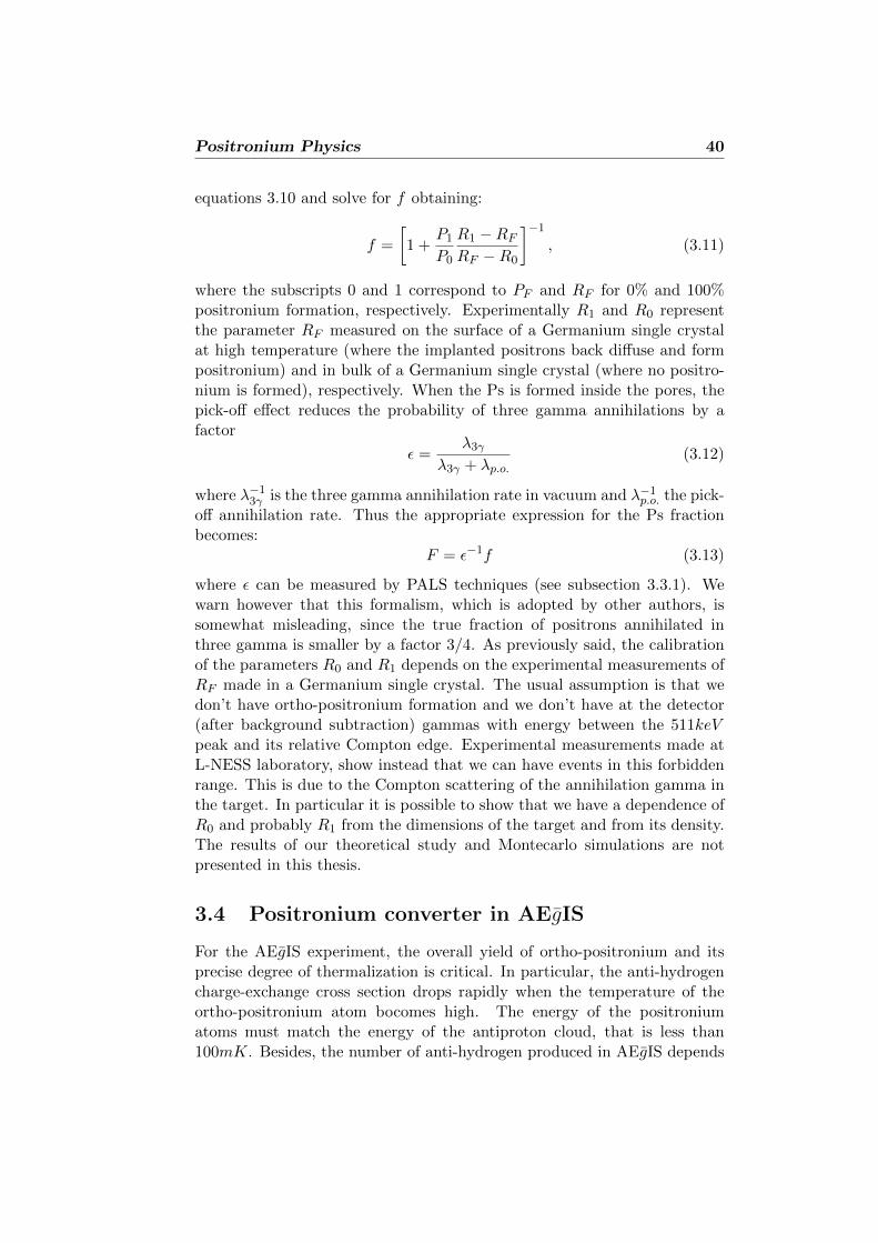
from the number of ortho-positronium atoms emitted by the converter andlaser excited. A schematic view of this part of the AEgIS apparatus is shownin figure 3.13.
Figure 3.13: Scheme of the AEgIS apparatus for antihydrogen production.The positrons are sent to the porous target and then converted to positro-nium atoms (Ps). Two laser pulses hit the positronium atoms in order toexcite them. Rydberg positronium atoms (Ps∗) arrive to the antiprotontraps where they can produce antihydrogen.
For the laser excitation process to be efficient the positronium cloud mustbe spatially localized and with appropriate velocity (corrisponding to feweV). The velocity depends upon the characteristics of the converter material,its pore structure, the implantation depth and the target temperature. Theuse of porous materials with pores connected to the target surface is funda-mental in order to have positronium thermalization and emission. The use ofmetallic and semi-metallic converters would certainly be more efficient fromthe point of view of positronium cooling, since a single collision of a positro-nium atom with a free electron at the surface of the metal can produce afractional energy loss of 50% thereby reducing the number of necessary colli-sions to less than about 100. On the other hand, pick-off annihilation lossesin a metal are expected to strongly reduce the flux of ortho-positroniumemerging from the pores. Nevertheless, the lack of experimental data onthis subject suggests that one should not a priori abandon any attempt touse a metallic converter.
The AEgIS collaboration is developping a new kind of porous metal tar-gets made of compressed metal microspheres (see section 3.4.1). In thesekind of converters the pores are connected each other and with the target sur-face, but are disordered. The ortho-positronium atoms are thus expected tobe emitted isotropically in vacuum. The only way to compensate the ortho-

Positronium Physics 42
postronium loss by solid angle is by having a high positronium formationyield. Another problem is that disordered pores do not permit the tuningof the emitted ortho-positronium energy. In addition, this energy dependson the pore shape, its diameter and the positron penetration depth.
Insulators must also be considered. In this case the positronium forma-tion yield is not too low and the pick-off annihilation losses do not reducedrastically the flux of the emitted ortho-positronium. Several groups havestudied porous insulator materials with disordered and interconnected pores.In particular the AEgIS collaboration is studying a wide set of converterswith ordered and disordered porosity, i.e. Alumina with ordered nanochan-nels (Whatman R© membrane), Vycor glasses, MOFs, aerogel/xerogel andMACS[62]. Insulators must however be considered with care because ofspace charge effect in the AEGIS experimental setup.
3.4.1 Metal/SiO2 Microspheres
The Chemistry Department of the Universita degli Studi di Milano is devel-oping new kinds of porous metallic targets. The common idea, at the baseof all these samples, is the compression of metallic micro-spheres in orderto orbtain a compact solid with disordered voids in the bulk and (impor-tant for the experiment) on the surface. These targets should be able toform positronium that, after many collisions on the pores wall, can escapefrom the solid as cold ortho-positronium. The metallic nature of the sampleprevents the possibility of electric breakdown triggered by the high positrondensity bunch in AEgIS . Two TEM images of two microspheres targets(gold and silver) are shown in figure 3.14.
Figure 3.14: TEM picture of the gold (a) and silver (b) microspheres targetsurface.
Up to now, the AEgIS chemistry group is studying the possibility torealize a solid target made of silicon oxyde microspheres compressed, withintrinsic nanoporosity [63]. Thus, this sample should present two set of
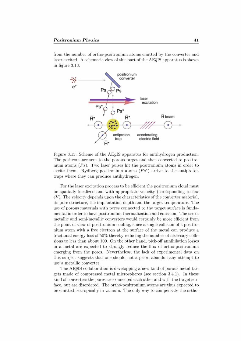
Positronium Physics 43
voids with two different diameter ranges: micro voids between the spheresand nano or subnano voids in the spheres as shown in figure 3.15.
Figure 3.15: TEM picture of the porous silica microspheres condensate. Thepicture shows the two set of voids of this target: micro voids between thespheres and nano or subnano voids in the spheres.
3.4.2 Whatman R© membrane
The Whatman R© Anopore inorganic membrane is composed of high purityanodic alumina (Al2O3), electrochemically manufactured, with a precise,non-deformable honeycomb pore structure with no lateral crossovers be-tween individual pores. This commercial membrane is supplied in the formof disks, bonded to an annular polypropylene ring. The minimum diametersof the pores is of about 20nm. The target thickness is 60µm. In figure 3.16,the pore structure of the Whatman R© membrane is shown. Van Petegem etal. have demostrated experimentally that in single-crystalline Al2O3, bulkpositronium is not formed but positronium emission from the surface hasbeen observed [41]. This is in agreement with the observed positronium for-mation in polycristalline Alumina powders where the positronium formationis observed on the wall of the free volumes between the powder grains [64].Thus in the Whatman R© anopore membrane, the well-ordered channel poros-ity combined with positronium formation in the “bulk” of anodic Aluminasamples would eventually lead to high positronium yield and positroniumemission into vacuum. In a similar sample, N. Djourelov et al. [64], from

Positronium Physics 44
Figure 3.16: (a) Schematic representation of anodic alumina structure and(b) electron microscopy image of the surface of an anodic Al2O3 with pore’sdiameter of about 70nm.
the 3γ method analysis, estimate that the 20% of all the injected positronswill form ortho-positronium.
3.4.3 Vycor glass
Vycor porous glass is an open cell, pourous glass formed by 96% of silicondioxide. The homogeneous pore diameters can be controlled to averagebetween 40 and 200 Angstroms. 3 γ measurements made in the Como L-NESS laboratory shows a positronium formation yield of about 10%-20%.Advantages of Vycor porous glass for positron to positronium converterinclude rigidity, chemical inertness, high temperature capability, superiorthermal shock resistance, and controlled microporosity. In the other hand,electric breakdown is a disadvantage.
3.4.4 MOFs
Other materials considered as converters are the Metal-Organic frameworks(MOFs). These are crystalline compounds consisting of metal ions or clus-ters coordinated to rigid organic molecules to form one, two, or three-dimensional structures that can be porous (in our case we have a quasi-cubicgrains with a side of about 50µm). In particular we considered MOF-177.This kind of MOF consists of octahedral Zn4 carboxylate clusters linked toorganic groups. Its surface area was determined to be an unprecedented4500m2/g, which exceeds the surface areas of other MOFs, carbon materi-als, and zeolites. Its density is 4.27·10−1g/cm3. The open spaces are regularand have dimensions of a few nanometers. Figure 3.17 shows the structureof MOF-177. Potentially, the positronium formed in the open spaces can bedrifted to the suface and thus emitted in vacuum. The regularity of the voids

Positronium Physics 45
Figure 3.17: The Isoreticular Metal Organic Frameworks (IMOFS) MOF-177
may give directionality at the outgoing positronium. The 3γ measurements,made in Como L-NESS laboratories, show a formation positronium yield ofabout 5%-10%. We don’t have, at the moment, measures in MOF-177 thatindicate the directionality of the outgoing positronium atoms.
3.4.5 Aerogel/Xerogel
Aerogel is a manufactured material with the lowest bulk density of anyknown porous solid. It is derived from a gel in which the liquid component ofthe gel has been replaced with a gas. The result is an extremely low-densitysolid with several remarkable properties, most notably its effectiveness asa thermal insulator. Aerogel was first created by Samuel Stephens Kistlerin 1931 [65], as a result of a bet with Charles Learned over who could re-place the liquid in “jellies” with gas without causing shrinkage. The firstaerogels were produced from silica gels. Kistler’s later work involved aero-gels based on alumina, chromia and tin oxide. Carbon aerogels were firstdeveloped in the late 1980s. The aerogel samples available to the AEgIScollaboration are Aerogel-150 and AerogelC-20. The number indicates theaerogel density in mg/cm3. The Aerogel samples of 20mg/cm3 were dopedwith C atoms (0.67% atoms of graphite). All aerogel used in AEgIS aresilica aerogel. Silica aerogel is the most common type of aerogel and themost extensively studied and used. It is a silica-based substance, derivedfrom silica gel. The average pore diameter is ' 1nm ≤ d ≤ 150nm and theporosity8 lays between 93% and 99%. Another target tested by the AEgIScollaboration is Xerogel. A Xerogel is a solid formed from a gel by drying itwith unhindered shrinkage. Xerogels usually retain high porosity (25%) and
8Defined as the vacuum to matter volume ratio in a porous material.

Positronium Physics 46
enormous surface area, along with very small pore size (1 − 10nm). Nitro-gen absorption measurements showed the presence of a bimodal distributionof pores, featuring nanopores (below 2nm) and mesopores (between 20nmand 50nm). The number density of the small pores was strongly dominant(150:1). Figure 3.18 shows the Xerogel-85 target during the 3γ mesurementsmade in the L-NESS laboratory. Also in Xerogel, the number 85 indicatesthe sample density of 85mg/cm3. Germanate Xerogel is a normal aerogelin which some silicon atoms are replaced by germanium. In these Aero-
Figure 3.18: The Xerogel-85 target during the 3γ mesurements made in theL-NESS laboratory.
gel/Xerogel targets it is not possible to do PALS measurements due to theirvery low density (too many long lifetime components). However 3γ mesure-ments made in L-NESS laboraties shows that the positronium formationyield of Aerogel and Xerogel is very high, between 45% and 60%. The onlyone that produces “only” about 10%-20% is the Germanate Xerogel sample.Future TOF measurements are necessary in order to measure the velocityof the outgoing positronium atoms.
3.4.6 MACS
The Mesoporous Amorphous Calcium Silicate (MACS) are synthesized us-ing mesoporous silica grains, structured by esadecilammonium hexadecylammonium - trimetilbenzene mixed micelles and calcined at 550C in air.The MACS shows a well-defined mesoporous structure with high specificsurface area. The pores, with a cylindrical shape in the original material, arelocally deformed by compression. Other than the structural mesoporosity,the targets show a variable macroporosity (diameter greater than 90nm).In AEgIS we test two different MACS with two different macoporosities,
Positronium Physics 47
named MACS-A and MACS-B. The first macroporosity has a density of1.5cm3/g and the second one has 0.5cm3/g. From PALS measurementsmade in the positron laboratory at Politecnico di Milano, we have esti-mated (using the Tao-Eldrup model [46]) two different mean pore size9 inMACS-A and MACS-B, respectively R = 6.9± 1nm and R = 5.5± 0.7nm.3γ measurements made at L-NESS laboratory shows a positronium forma-tion yield of about 35%-50% for both samples. MACS are the samples thatproduce more positronium after Aerogel/Xerogel. Moreover the advantageof MACS over Aerogel/Xerogel is due to the regularity of the pore and of thegeometry, as they forms nanochannel, which is fundamental for the AEgISpurpose.
3.4.7 Ordered nano-channels Si/SiO2
The Trento group of the AEgIS collaboration developped a novel structurewith ordered nano-channels perpendicular to the surface [66]. Nano-channelshave been produced by selective etching in silicon and oxidized in air atdifferent temperatures and times. A scanning electron microscopy pictureof the converter surface is shown in figure 3.19. In that sample, holes of5-8 nm in diameter are present, and are spaced by about the same distanceof 5-8 nm. The synthesis of the converter was optimized by maximizing
Figure 3.19: SEM picture of the Si/SiO2 nano-channels converter surfacewith 5− 8nm pores.
9With R we indicate the porous mean radius.
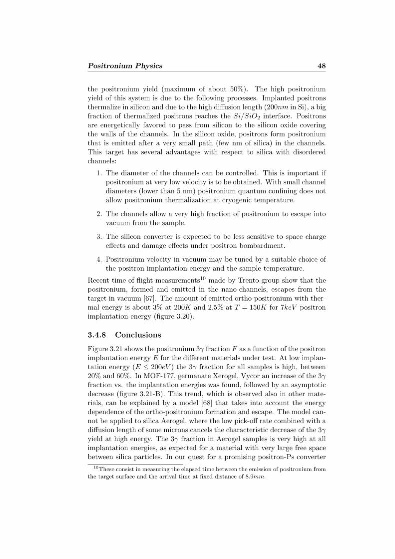
Positronium Physics 48
the positronium yield (maximum of about 50%). The high positroniumyield of this system is due to the following processes. Implanted positronsthermalize in silicon and due to the high diffusion length (200nm in Si), a bigfraction of thermalized positrons reaches the Si/SiO2 interface. Positronsare energetically favored to pass from silicon to the silicon oxide coveringthe walls of the channels. In the silicon oxide, positrons form positroniumthat is emitted after a very small path (few nm of silica) in the channels.This target has several advantages with respect to silica with disorderedchannels:
1. The diameter of the channels can be controlled. This is important ifpositronium at very low velocity is to be obtained. With small channeldiameters (lower than 5 nm) positronium quantum confining does notallow positronium thermalization at cryogenic temperature.
2. The channels allow a very high fraction of positronium to escape intovacuum from the sample.
3. The silicon converter is expected to be less sensitive to space chargeeffects and damage effects under positron bombardment.
4. Positronium velocity in vacuum may be tuned by a suitable choice ofthe positron implantation energy and the sample temperature.
Recent time of flight measurements10 made by Trento group show that thepositronium, formed and emitted in the nano-channels, escapes from thetarget in vacuum [67]. The amount of emitted ortho-positronium with ther-mal energy is about 3% at 200K and 2.5% at T = 150K for 7keV positronimplantation energy (figure 3.20).
3.4.8 Conclusions
Figure 3.21 shows the positronium 3γ fraction F as a function of the positronimplantation energy E for the different materials under test. At low implan-tation energy (E ≤ 200eV ) the 3γ fraction for all samples is high, between20% and 60%. In MOF-177, germanate Xerogel, Vycor an increase of the 3γfraction vs. the implantation energies was found, followed by an asymptoticdecrease (figure 3.21-B). This trend, which is observed also in other mate-rials, can be explained by a model [68] that takes into account the energydependence of the ortho-positronium formation and escape. The model can-not be applied to silica Aerogel, where the low pick-off rate combined with adiffusion length of some microns cancels the characteristic decrease of the 3γyield at high energy. The 3γ fraction in Aerogel samples is very high at allimplantation energies, as expected for a material with very large free spacebetween silica particles. In our quest for a promising positron-Ps converter
10These consist in measuring the elapsed time between the emission of positronium fromthe target surface and the arrival time at fixed distance of 8.9mm.
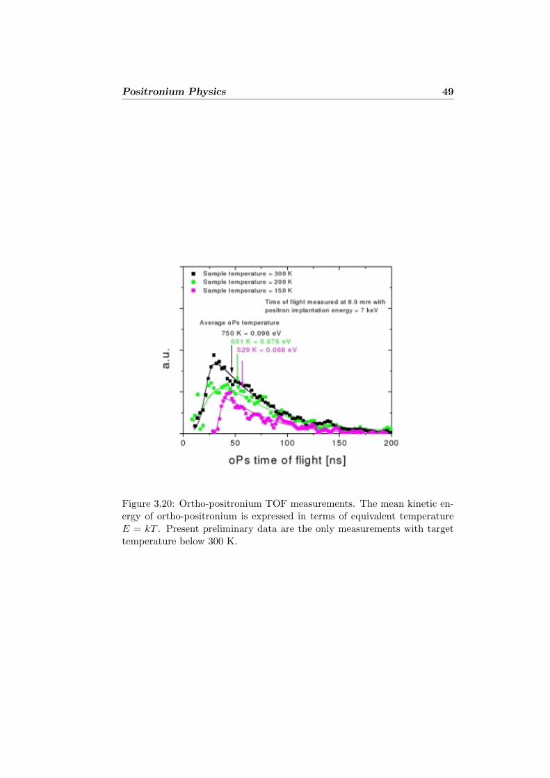
Positronium Physics 49
Figure 3.20: Ortho-positronium TOF measurements. The mean kinetic en-ergy of ortho-positronium is expressed in terms of equivalent temperatureE = kT . Present preliminary data are the only measurements with targettemperature below 300 K.
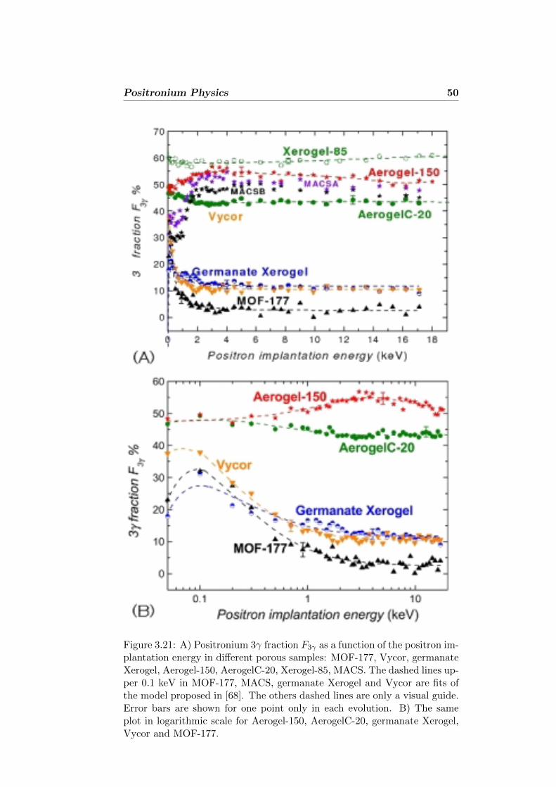
Positronium Physics 50
Figure 3.21: A) Positronium 3γ fraction F3γ as a function of the positron im-plantation energy in different porous samples: MOF-177, Vycor, germanateXerogel, Aerogel-150, AerogelC-20, Xerogel-85, MACS. The dashed lines up-per 0.1 keV in MOF-177, MACS, germanate Xerogel and Vycor are fits ofthe model proposed in [68]. The others dashed lines are only a visual guide.Error bars are shown for one point only in each evolution. B) The sameplot in logarithmic scale for Aerogel-150, AerogelC-20, germanate Xerogel,Vycor and MOF-177.
Positronium Physics 51
to be chosen in the AEgIS experiment, the collaboration has tested a seriesof materials with known open porosity. We have found that the highestformation of positronium occurs in Xerogel, Aerogel and MACS. However,high formation is not the only important factor. It must be reminded thatpositronium is emitted into the pores with an initial kinetic energy of theorder of a few eV. Since our goal is to obtain ortho-positronium in the freespace with energies of the order of 10−2eV , it is necessary that the positro-nium suffers a large number of collisions with the walls of the pores beforeemerging in the free space outside the target. This means that the usefulortho-positronium fraction must come from the deep regions of the target.This is certainly not the case of germanate Xerogel, where ortho-positroniumappears to be strongly quenched in the pores. The reason is the presencein this material of a dense distribution of very small pores, probably witha low degree of interconnections, which act as dominant ortho-positroniumcages. Most probably, this situation also occurs in Vycor. MOF-177 is anew material; there is no previous information of its ability in producingpositronium. The experiments done in L-NESS laboratories show that, inspite of its very large free volume, this material is not really interesting as aconverter. On the contrary, low-density Aerogel and Xerogel are a promisingtarget candidate under two aspects: high formation and long survival timeof ortho-positronium inside the pores. Finally MACS is the more interest-ing material because it has high positronium formation yield and a regularscructures of its nanopores. These nano-channels could give to positroniumatoms the correct directionality request in the AEgIS experiments. Anotherimportant target is the ordered nano-channeled Si/SiO2 converter. In thiscase the yield is not very high but have many advantage like the possibilityto make directional channels and its better electrical conduction proprieties.Additionally we have much informations about this target like TOF and“low” temperature measurements. Up to date, except for the ordered nano-channeled Si/SiO2 converter, it was not possible to measure the kineticenergy of ortho-positronium outside the target. TOF measurements of theemitted ortho-positronium are highly desirable for finding the best compro-mise. At the moment all the presented targets are possible candidates.
3.5 Positronium formation in extreme conditions
In the previous sections we analysed the positronium formation and ther-malization in solids without considering some important experimental con-dictions fixed by the AEgIS apparatus:
• The first one is that the converter is located in a 1T magnetic field.In a magnetic field the ortho-positronium state with spin componentSz = 0 is mixed with the para-positronium singlet state, resulting in areduction of the self annihilation lifetime. On the contrary the lifetime
Positronium Physics 52
of the orthopositronium states with Sz = ±1 are not affected by themagnetic field, therefore the maximum expected yield reduction in amagnetic field of 1T is one third of the ortho-positronium fraction.
• Another experimental condition is that the converter is at cryogenictemperature of about 100mK. Theoretically, as described previously,the converter temperature should not influence the positronium pro-duction mechanism. As of today we don’t have any measurement ofpositronium formation at so low temperature. The Trento group hasshown that, in the case of ordered nano-channeled Si/SiO2 target, wehave a decrease of positronium formation yield when the temperaturedecreases from 300K to 150K. This effect is under investigation.
• The last experimental request is the amount of positron irradiationdose on the converter. There is the possibility that the intense positronbunches can damage the porous structures and so decrease the ortho-positronium yield. In order to understand the entity of the radiationdamage I designed and realized an electron beam, named eBEAM, thatoffers the same AEgIS radiation dose (in terms of particles number andenergy) but in less time with respect to a typical positron beam. Thedescription of the apparatus will be presented in chapter 4.
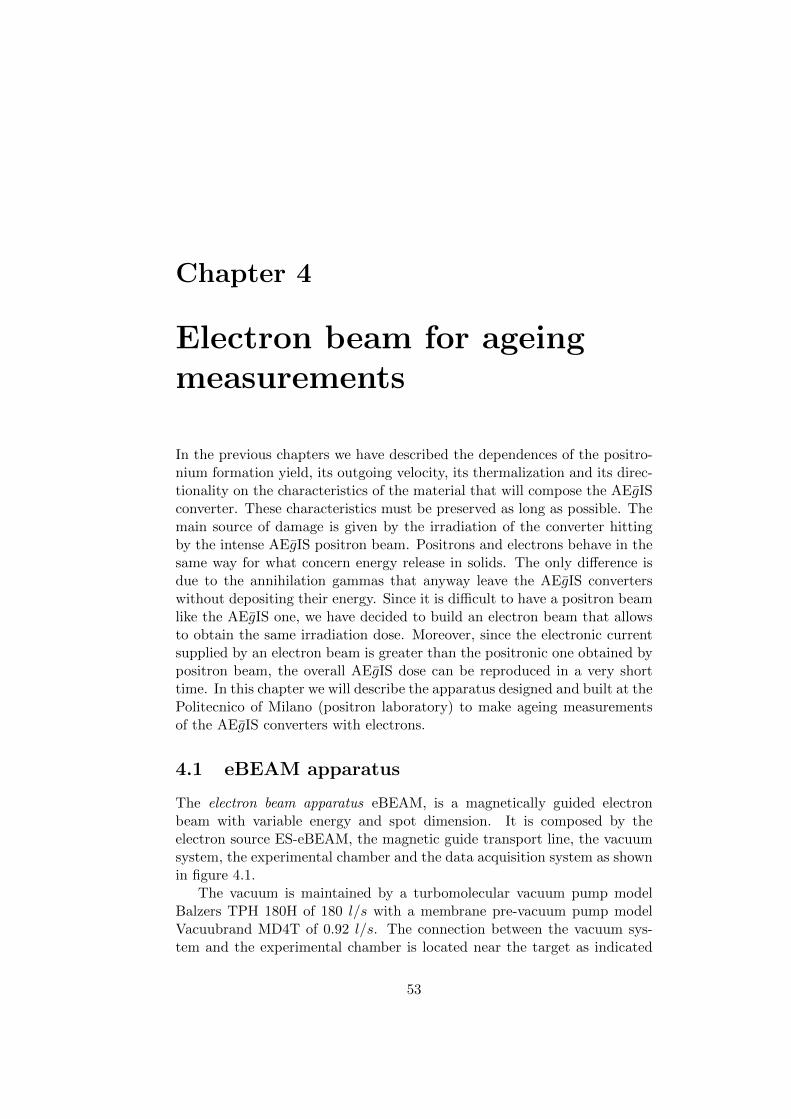
Chapter 4
Electron beam for ageingmeasurements
In the previous chapters we have described the dependences of the positro-nium formation yield, its outgoing velocity, its thermalization and its direc-tionality on the characteristics of the material that will compose the AEgISconverter. These characteristics must be preserved as long as possible. Themain source of damage is given by the irradiation of the converter hittingby the intense AEgIS positron beam. Positrons and electrons behave in thesame way for what concern energy release in solids. The only difference isdue to the annihilation gammas that anyway leave the AEgIS converterswithout depositing their energy. Since it is difficult to have a positron beamlike the AEgIS one, we have decided to build an electron beam that allowsto obtain the same irradiation dose. Moreover, since the electronic currentsupplied by an electron beam is greater than the positronic one obtained bypositron beam, the overall AEgIS dose can be reproduced in a very shorttime. In this chapter we will describe the apparatus designed and built at thePolitecnico of Milano (positron laboratory) to make ageing measurementsof the AEgIS converters with electrons.
4.1 eBEAM apparatus
The electron beam apparatus eBEAM, is a magnetically guided electronbeam with variable energy and spot dimension. It is composed by theelectron source ES-eBEAM, the magnetic guide transport line, the vacuumsystem, the experimental chamber and the data acquisition system as shownin figure 4.1.
The vacuum is maintained by a turbomolecular vacuum pump modelBalzers TPH 180H of 180 l/s with a membrane pre-vacuum pump modelVacuubrand MD4T of 0.92 l/s. The connection between the vacuum sys-tem and the experimental chamber is located near the target as indicated
53
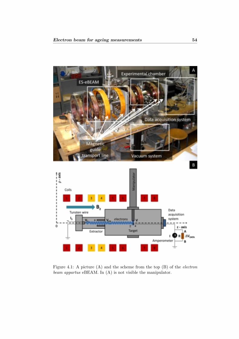
Electron beam for ageing measurements 54
Figure 4.1: A picture (A) and the scheme from the top (B) of the electronbeam appartus eBEAM. In (A) is not visible the manipulator.
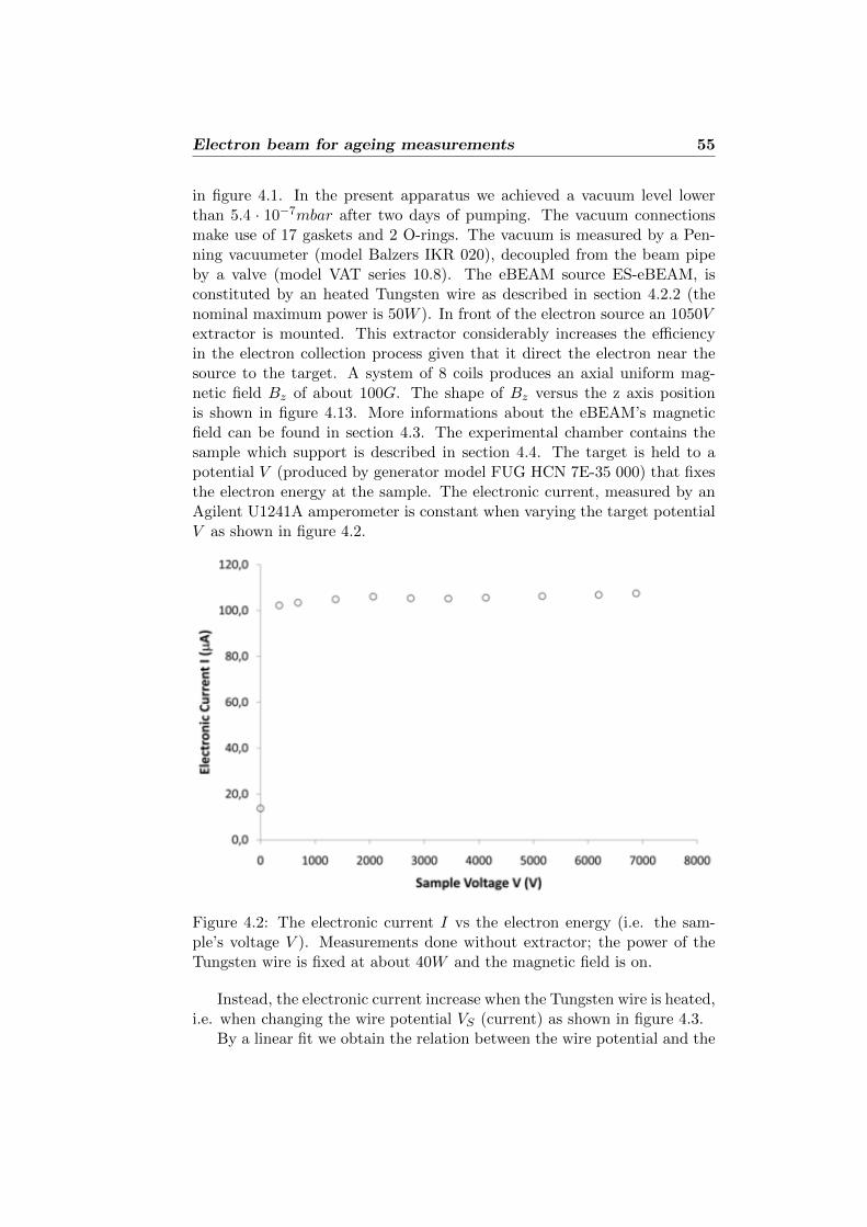
Electron beam for ageing measurements 55
in figure 4.1. In the present apparatus we achieved a vacuum level lowerthan 5.4 · 10−7mbar after two days of pumping. The vacuum connectionsmake use of 17 gaskets and 2 O-rings. The vacuum is measured by a Pen-ning vacuumeter (model Balzers IKR 020), decoupled from the beam pipeby a valve (model VAT series 10.8). The eBEAM source ES-eBEAM, isconstituted by an heated Tungsten wire as described in section 4.2.2 (thenominal maximum power is 50W ). In front of the electron source an 1050Vextractor is mounted. This extractor considerably increases the efficiencyin the electron collection process given that it direct the electron near thesource to the target. A system of 8 coils produces an axial uniform mag-netic field Bz of about 100G. The shape of Bz versus the z axis positionis shown in figure 4.13. More informations about the eBEAM’s magneticfield can be found in section 4.3. The experimental chamber contains thesample which support is described in section 4.4. The target is held to apotential V (produced by generator model FUG HCN 7E-35 000) that fixesthe electron energy at the sample. The electronic current, measured by anAgilent U1241A amperometer is constant when varying the target potentialV as shown in figure 4.2.
Figure 4.2: The electronic current I vs the electron energy (i.e. the sam-ple’s voltage V ). Measurements done without extractor; the power of theTungsten wire is fixed at about 40W and the magnetic field is on.
Instead, the electronic current increase when the Tungsten wire is heated,i.e. when changing the wire potential VS (current) as shown in figure 4.3.
By a linear fit we obtain the relation between the wire potential and the
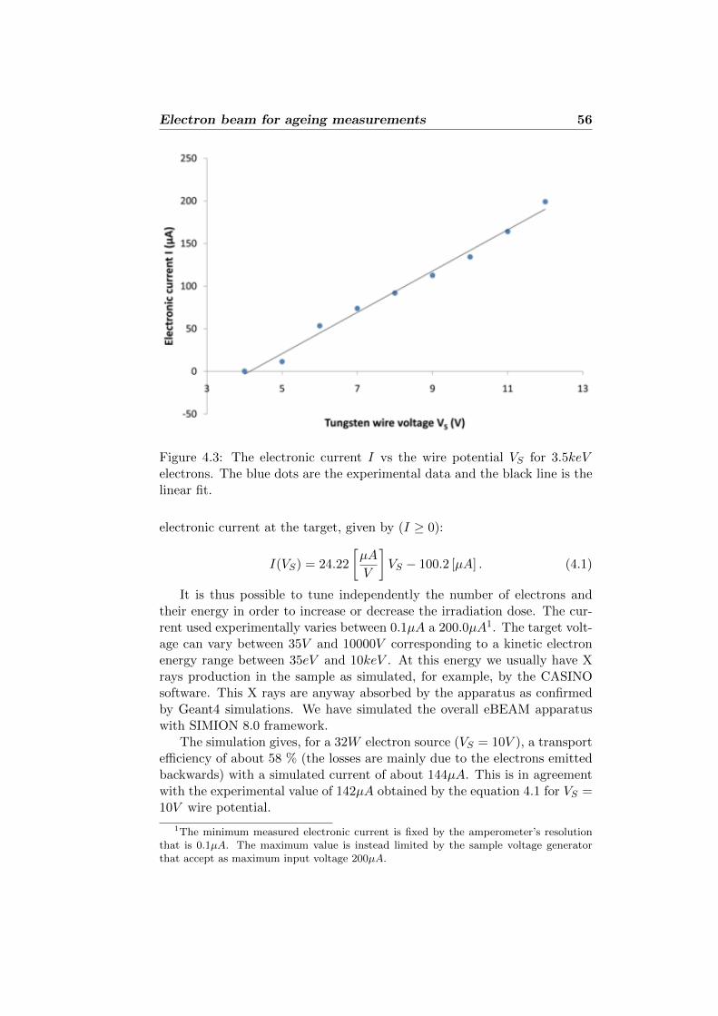
Electron beam for ageing measurements 56
Figure 4.3: The electronic current I vs the wire potential VS for 3.5keVelectrons. The blue dots are the experimental data and the black line is thelinear fit.
electronic current at the target, given by (I ≥ 0):
I(VS) = 24.22
[µA
V
]VS − 100.2 [µA] . (4.1)
It is thus possible to tune independently the number of electrons andtheir energy in order to increase or decrease the irradiation dose. The cur-rent used experimentally varies between 0.1µA a 200.0µA1. The target volt-age can vary between 35V and 10000V corresponding to a kinetic electronenergy range between 35eV and 10keV . At this energy we usually have Xrays production in the sample as simulated, for example, by the CASINOsoftware. This X rays are anyway absorbed by the apparatus as confirmedby Geant4 simulations. We have simulated the overall eBEAM apparatuswith SIMION 8.0 framework.
The simulation gives, for a 32W electron source (VS = 10V ), a transportefficiency of about 58 % (the losses are mainly due to the electrons emittedbackwards) with a simulated current of about 144µA. This is in agreementwith the experimental value of 142µA obtained by the equation 4.1 for VS =10V wire potential.
1The minimum measured electronic current is fixed by the amperometer’s resolutionthat is 0.1µA. The maximum value is instead limited by the sample voltage generatorthat accept as maximum input voltage 200µA.
Electron beam for ageing measurements 57
4.2 The electron source
The usual way to produce electrons is by means of an electronic gun. In orderto understand the operation of this machine and to improve its performance,we designed and built two electronic guns. The first one, conceived as a testsource (Test Electron Source, TES-eBEAM), was designed for a low vacuumsystem and an operational time of only few minutes. The second one isinstead the final eBEAM electron source (Electron Source, ES-eBEAM). Inthe following sections we will present the design and the experimental testsof the two electron sources.
4.2.1 TES-eBEAM
The TES-eBEAM design and a picture of the apparatus at the Politecnicodi Milano positron laboratory are shown in figure 4.4.
The electronic scheme of the electron source is depicted in figure 4.4 andis quite simple. A tungsten wire is heated by Joule effect to a temperature of1000−2000K. This is achieved by the current generator G1 that produces aDC current IS between 0 and 4A. The positive pole is connected at ground.Thus, the wire is repulsive from the electrons point of view. They are sodriven to the positive charged electrode E . This electrode is powered by thehigh voltage generator G2 that produces a positive potential V , attractivefor the emitted electrons. The distance between the wire and the electrodeis about 200mm. This small distance does not require the presence of anextractor electrode in front of the wire in order to reduce electron losses.Theelectronic current generated by the electrons emitted by the source is mea-sured by an analogic amperometer A with resolution of 0.5µA. The electronenergy spectrum of the source depends on:
• the negative potential between the wire and ground VS ,
• the positive potential on the target V ,
• the kinetic energy of the electrons when they are thermoionically emit-ted by the wire (temperature dependent).
In order to understand the shape of the electron energy spectrum, we devel-oped a Monte Carlo simulation of electron emission from Tungsten wire [69].The details are reported in appendix A where we also report the analytical

Electron beam for ageing measurements 58
Figure 4.4: The TES-eBEAM apparatus. (A) the design (B) the elecronsource during the experimental tests (C) the electronic scheme.
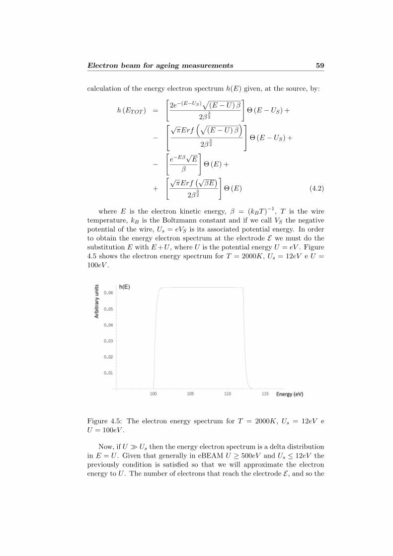
Electron beam for ageing measurements 59
calculation of the energy electron spectrum h(E) given, at the source, by:
h (ETOT ) =
[2e−(E−US)
√(E − U)β
2β32
]Θ (E − US) +
−
√πErf(√
(E − U)β)
2β32
Θ (E − US) +
−
[e−Eβ
√E
β
]Θ (E) +
+
[√πErf
(√βE)
2β32
]Θ (E) (4.2)
where E is the electron kinetic energy, β = (kBT )−1, T is the wiretemperature, kB is the Boltzmann constant and if we call VS the negativepotential of the wire, Us = eVS is its associated potential energy. In orderto obtain the energy electron spectrum at the electrode E we must do thesubstitution E with E+U , where U is the potential energy U = eV . Figure4.5 shows the electron energy spectrum for T = 2000K, Us = 12eV e U =100eV .
Figure 4.5: The electron energy spectrum for T = 2000K, Us = 12eV eU = 100eV .
Now, if U Us then the energy electron spectrum is a delta distributionin E = U . Given that generally in eBEAM U ≥ 500eV and Us ≤ 12eV thepreviously condition is satisfied so that we will approximate the electronenergy to U . The number of electrons that reach the electrode E , and so the
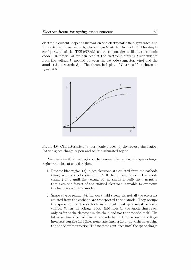
Electron beam for ageing measurements 60
electronic current, depends instead on the electrostatic field generated andin particular, in our case, by the voltage V at the electrode E . The simpleconfiguration of the TES-eBEAM allows to consider it like a thermionicdiode. In particular we can predict the electronic current I dependencefrom the voltage V applied between the cathode (tungsten wire) and theanode (the electrode E). The theoretical plot of I versus V is shown infigure 4.6.
Figure 4.6: Characteristic of a thermionic diode: (a) the reverse bias region,(b) the space charge region and (c) the saturated region.
We can identify three regions: the reverse bias region, the space-chargeregion and the saturated region.
1. Reverse bias region (a): since electrons are emitted from the cathode(wire) with a kinetic energy K > 0 the current flows in the anode(target) only until the voltage of the anode is sufficiently negativethat even the fastest of the emitted electrons is unable to overcomethe field to reach the anode.
2. Space charge region (b): for weak field strengths, not all the electronsemitted from the cathode are transported to the anode. They occupythe space around the cathode in a cloud creating a negative spacecharge. When the voltage is low, field lines for the anode thus reachonly as far as the electrons in the cloud and not the cathode itself. Thelatter is thus shielded from the anode field. Only when the voltageincreases can the field lines penetrate further into the cathode causingthe anode current to rise. The increase continues until the space charge
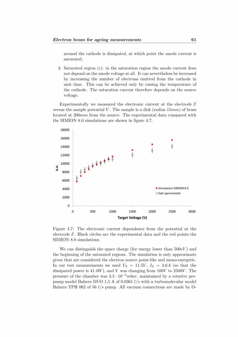
Electron beam for ageing measurements 61
around the cathode is dissipated, at which point the anode current issaturated.
3. Saturated region (c): in the saturation region the anode current doesnot depend on the anode voltage at all. It can nevertheless be increasedby increasing the number of electrons emitted from the cathode inunit time. This can be achieved only by raising the temperature ofthe cathode. The saturation current therefore depends on the sourcevoltage.
Experimentally we measured the electronic current at the electrode Eversus the sample potential V . The sample is a disk (radius 15mm) of brasslocated at 200mm from the source. The experimental data compared withthe SIMION 8.0 simulations are shown in figure 4.7.
Figure 4.7: The electronic current dependence from the potential at theelectrode E . Black circles are the experimental data and the red points theSIMION 8.0 simulations.
We can distinguish the space charge (for energy lower than 500eV ) andthe beginning of the saturated regions. The simulation is only approximategiven that are considered the electron source point-like and mono-energetic.In our test measurements we used VS = 11.5V , IS = 3.6A (so that thedissipated power is 41.4W ), and V was changing from 100V to 2500V . Thepressure of the chamber was 3.5 · 10−5mbar, maintained by a rotative pre-pump model Balzers DUO 1,5 A of 0.0361 l/s with a turbomolecular modelBalzers TPH 062 of 56 l/s pump. All vacuum connections are made by O-
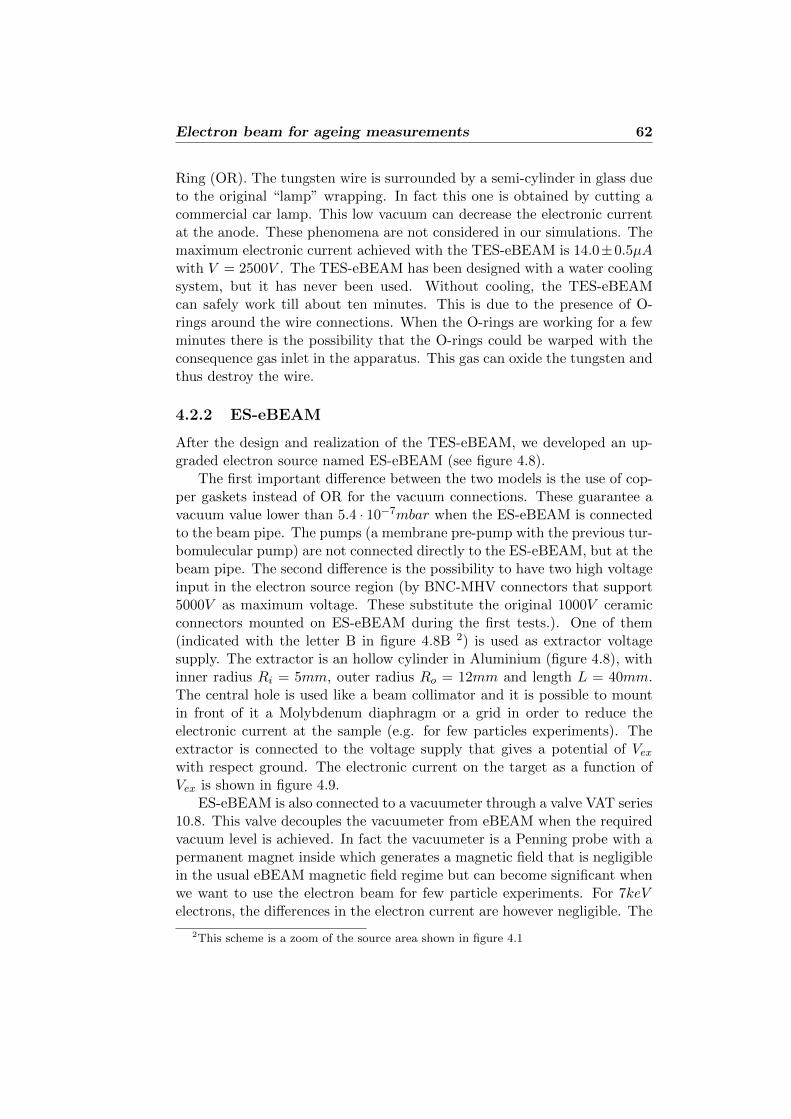
Electron beam for ageing measurements 62
Ring (OR). The tungsten wire is surrounded by a semi-cylinder in glass dueto the original “lamp” wrapping. In fact this one is obtained by cutting acommercial car lamp. This low vacuum can decrease the electronic currentat the anode. These phenomena are not considered in our simulations. Themaximum electronic current achieved with the TES-eBEAM is 14.0±0.5µAwith V = 2500V . The TES-eBEAM has been designed with a water coolingsystem, but it has never been used. Without cooling, the TES-eBEAMcan safely work till about ten minutes. This is due to the presence of O-rings around the wire connections. When the O-rings are working for a fewminutes there is the possibility that the O-rings could be warped with theconsequence gas inlet in the apparatus. This gas can oxide the tungsten andthus destroy the wire.
4.2.2 ES-eBEAM
After the design and realization of the TES-eBEAM, we developed an up-graded electron source named ES-eBEAM (see figure 4.8).
The first important difference between the two models is the use of cop-per gaskets instead of OR for the vacuum connections. These guarantee avacuum value lower than 5.4 · 10−7mbar when the ES-eBEAM is connectedto the beam pipe. The pumps (a membrane pre-pump with the previous tur-bomulecular pump) are not connected directly to the ES-eBEAM, but at thebeam pipe. The second difference is the possibility to have two high voltageinput in the electron source region (by BNC-MHV connectors that support5000V as maximum voltage. These substitute the original 1000V ceramicconnectors mounted on ES-eBEAM during the first tests.). One of them(indicated with the letter B in figure 4.8B 2) is used as extractor voltagesupply. The extractor is an hollow cylinder in Aluminium (figure 4.8), withinner radius Ri = 5mm, outer radius Ro = 12mm and length L = 40mm.The central hole is used like a beam collimator and it is possible to mountin front of it a Molybdenum diaphragm or a grid in order to reduce theelectronic current at the sample (e.g. for few particles experiments). Theextractor is connected to the voltage supply that gives a potential of Vexwith respect ground. The electronic current on the target as a function ofVex is shown in figure 4.9.
ES-eBEAM is also connected to a vacuumeter through a valve VAT series10.8. This valve decouples the vacuumeter from eBEAM when the requiredvacuum level is achieved. In fact the vacuumeter is a Penning probe with apermanent magnet inside which generates a magnetic field that is negligiblein the usual eBEAM magnetic field regime but can become significant whenwe want to use the electron beam for few particle experiments. For 7keVelectrons, the differences in the electron current are however negligible. The
2This scheme is a zoom of the source area shown in figure 4.1

Electron beam for ageing measurements 63
Figure 4.8: (A)The ES-eBeam electronic source during the preliminary testsin the Politecnico positron laboratory (the source is upside down comparedto the scheme B and C). (B) The ES-eBeam in the two extractor configura-tion. (C) The ES-eBeam in the one extractor configuration. The ES-eBeamoperates in absence of magnetic fields.
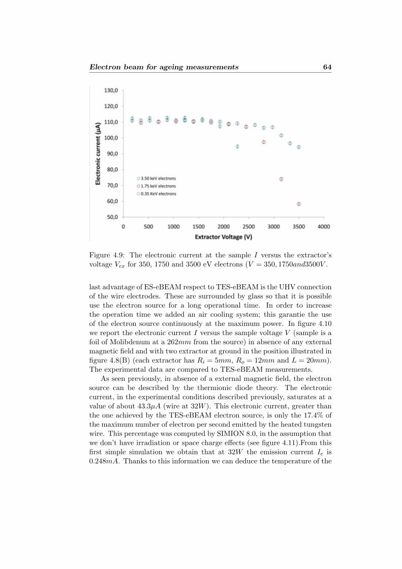
Electron beam for ageing measurements 64
Figure 4.9: The electronic current at the sample I versus the extractor’svoltage Vex for 350, 1750 and 3500 eV electrons (V = 350, 1750and3500V .
last advantage of ES-eBEAM respect to TES-eBEAM is the UHV connectionof the wire electrodes. These are surrounded by glass so that it is possibleuse the electron source for a long operational time. In order to increasethe operation time we added an air cooling system; this garantie the useof the electron source continuously at the maximum power. In figure 4.10we report the electronic current I versus the sample voltage V (sample is afoil of Molibdenum at a 262mm from the source) in absence of any externalmagnetic field and with two extractor at ground in the position illustrated infigure 4.8(B) (each extractor has Ri = 5mm, Ro = 12mm and L = 20mm).The experimental data are compared to TES-eBEAM measurements.
As seen previously, in absence of a external magnetic field, the electronsource can be described by the thermionic diode theory. The electroniccurrent, in the experimental conditions described previously, saturates at avalue of about 43.3µA (wire at 32W ). This electronic current, greater thanthe one achieved by the TES-eBEAM electron source, is only the 17.4% ofthe maximum number of electron per second emitted by the heated tungstenwire. This percentage was computed by SIMION 8.0, in the assumption thatwe don’t have irradiation or space charge effects (see figure 4.11).From thisfirst simple simulation we obtain that at 32W the emission current Ie is0.248mA. Thanks to this information we can deduce the temperature of the
Electron beam for ageing measurements 65
Figure 4.10: The electronic current versus the sample voltage V (sample isa foil of Molibdenum at a 262mm from the source) in absence of any exter-nal magnetic field. The experimental data are compared to TES-eBEAMmeasurements.
tungsten wire. In fact the Richardson’s law for the thermionic emission is:
Ie = AST 2e− WkBT (4.3)
where A = 1.2 · 10−6A/m2K2 is the Richardson’s constant, S ∼= 80mm2 isthe wire surface, T is the temperature of the wire, W = 4.5eV is the workfunction for the Tungsten, and kB is the Boltzmann’s constant. Now, if wesubstitute the numerical values, we obtain:
Ie(A) = 96AT 2e−52220KT (4.4)
By numerical integration of this equation for Ie = 2.48 · 10−4A we get T =1869K. In future it will be possible to compare this theoretical value withthe temperature measured for example with a pyrometer.
4.3 The magnetic guide field
The electrons emitted by the heated wire in the ES-eBEAM source are mag-netically guided to the sample support. In order to generate the appropriatemagnetic field we used a set of pre-existing coils (figure 4.1).
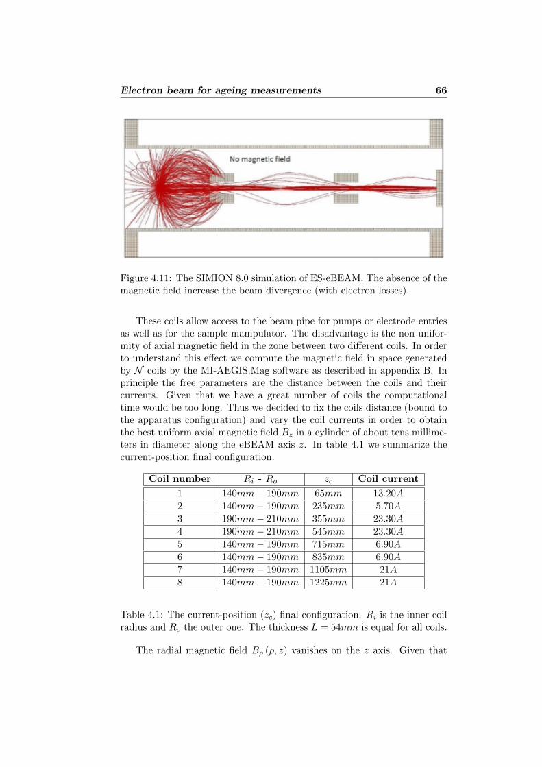
Electron beam for ageing measurements 66
Figure 4.11: The SIMION 8.0 simulation of ES-eBEAM. The absence of themagnetic field increase the beam divergence (with electron losses).
These coils allow access to the beam pipe for pumps or electrode entriesas well as for the sample manipulator. The disadvantage is the non unifor-mity of axial magnetic field in the zone between two different coils. In orderto understand this effect we compute the magnetic field in space generatedby N coils by the MI-AEGIS.Mag software as described in appendix B. Inprinciple the free parameters are the distance between the coils and theircurrents. Given that we have a great number of coils the computationaltime would be too long. Thus we decided to fix the coils distance (bound tothe apparatus configuration) and vary the coil currents in order to obtainthe best uniform axial magnetic field Bz in a cylinder of about tens millime-ters in diameter along the eBEAM axis z. In table 4.1 we summarize thecurrent-position final configuration.
Coil number Ri - Ro zc Coil current
1 140mm− 190mm 65mm 13.20A
2 140mm− 190mm 235mm 5.70A
3 190mm− 210mm 355mm 23.30A
4 190mm− 210mm 545mm 23.30A
5 140mm− 190mm 715mm 6.90A
6 140mm− 190mm 835mm 6.90A
7 140mm− 190mm 1105mm 21A
8 140mm− 190mm 1225mm 21A
Table 4.1: The current-position (zc) final configuration. Ri is the inner coilradius and Ro the outer one. The thickness L = 54mm is equal for all coils.
The radial magnetic field Bρ (ρ, z) vanishes on the z axis. Given that
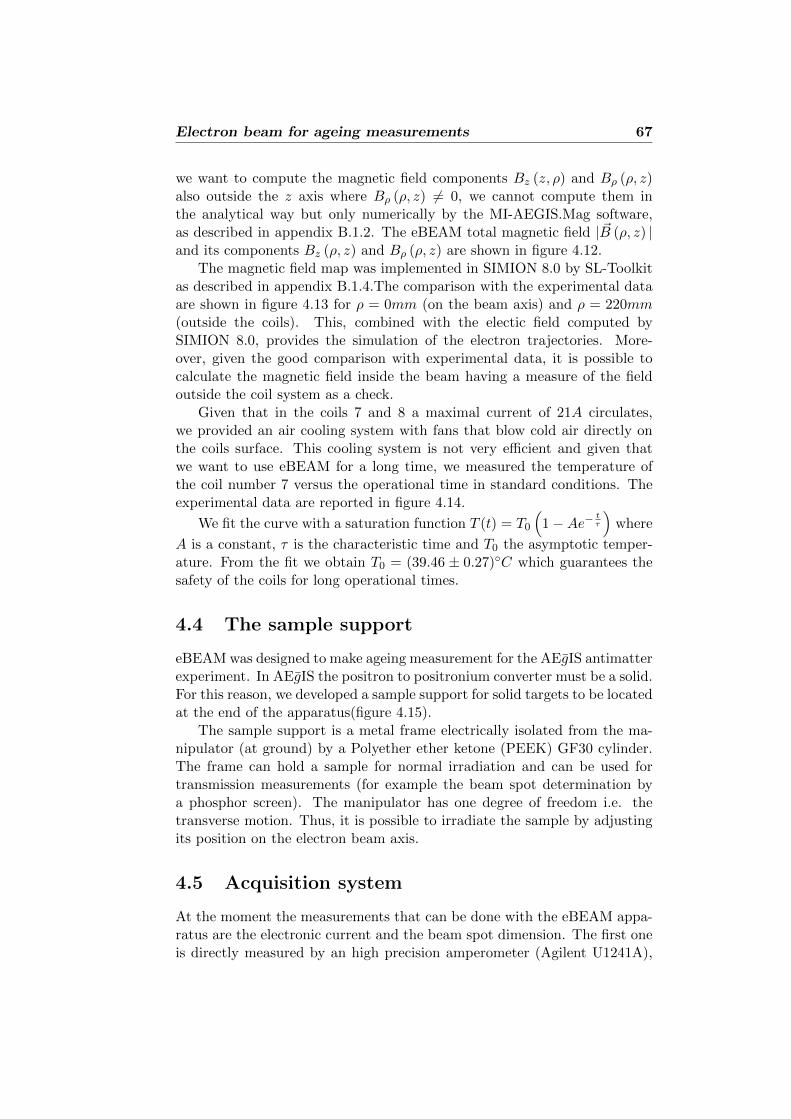
Electron beam for ageing measurements 67
we want to compute the magnetic field components Bz (z, ρ) and Bρ (ρ, z)also outside the z axis where Bρ (ρ, z) 6= 0, we cannot compute them inthe analytical way but only numerically by the MI-AEGIS.Mag software,as described in appendix B.1.2. The eBEAM total magnetic field | ~B (ρ, z) |and its components Bz (ρ, z) and Bρ (ρ, z) are shown in figure 4.12.
The magnetic field map was implemented in SIMION 8.0 by SL-Toolkitas described in appendix B.1.4.The comparison with the experimental dataare shown in figure 4.13 for ρ = 0mm (on the beam axis) and ρ = 220mm(outside the coils). This, combined with the electic field computed bySIMION 8.0, provides the simulation of the electron trajectories. More-over, given the good comparison with experimental data, it is possible tocalculate the magnetic field inside the beam having a measure of the fieldoutside the coil system as a check.
Given that in the coils 7 and 8 a maximal current of 21A circulates,we provided an air cooling system with fans that blow cold air directly onthe coils surface. This cooling system is not very efficient and given thatwe want to use eBEAM for a long time, we measured the temperature ofthe coil number 7 versus the operational time in standard conditions. Theexperimental data are reported in figure 4.14.
We fit the curve with a saturation function T (t) = T0
(1−Ae−
tτ
)where
A is a constant, τ is the characteristic time and T0 the asymptotic temper-ature. From the fit we obtain T0 = (39.46 ± 0.27)C which guarantees thesafety of the coils for long operational times.
4.4 The sample support
eBEAM was designed to make ageing measurement for the AEgIS antimatterexperiment. In AEgIS the positron to positronium converter must be a solid.For this reason, we developed a sample support for solid targets to be locatedat the end of the apparatus(figure 4.15).
The sample support is a metal frame electrically isolated from the ma-nipulator (at ground) by a Polyether ether ketone (PEEK) GF30 cylinder.The frame can hold a sample for normal irradiation and can be used fortransmission measurements (for example the beam spot determination bya phosphor screen). The manipulator has one degree of freedom i.e. thetransverse motion. Thus, it is possible to irradiate the sample by adjustingits position on the electron beam axis.
4.5 Acquisition system
At the moment the measurements that can be done with the eBEAM appa-ratus are the electronic current and the beam spot dimension. The first oneis directly measured by an high precision amperometer (Agilent U1241A),

Electron beam for ageing measurements 68
Figure 4.12: The eBEAM magnetic field computed by MI-AEGIS.Mag soft-ware. (A) is the total magnetic field | ~B (ρ, z) | (B) the axial componentBz (ρ, z) and (C) the radial one Bρ (ρ, z). The plots show as the axial mag-netic field on the beam axis is uniform and increase only near the target(z = 1m) in order to focus the particles.
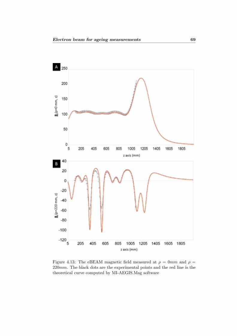
Electron beam for ageing measurements 69
Figure 4.13: The eBEAM magnetic field measured at ρ = 0mm and ρ =220mm. The black dots are the experimental points and the red line is thetheoretical curve computed by MI-AEGIS.Mag software
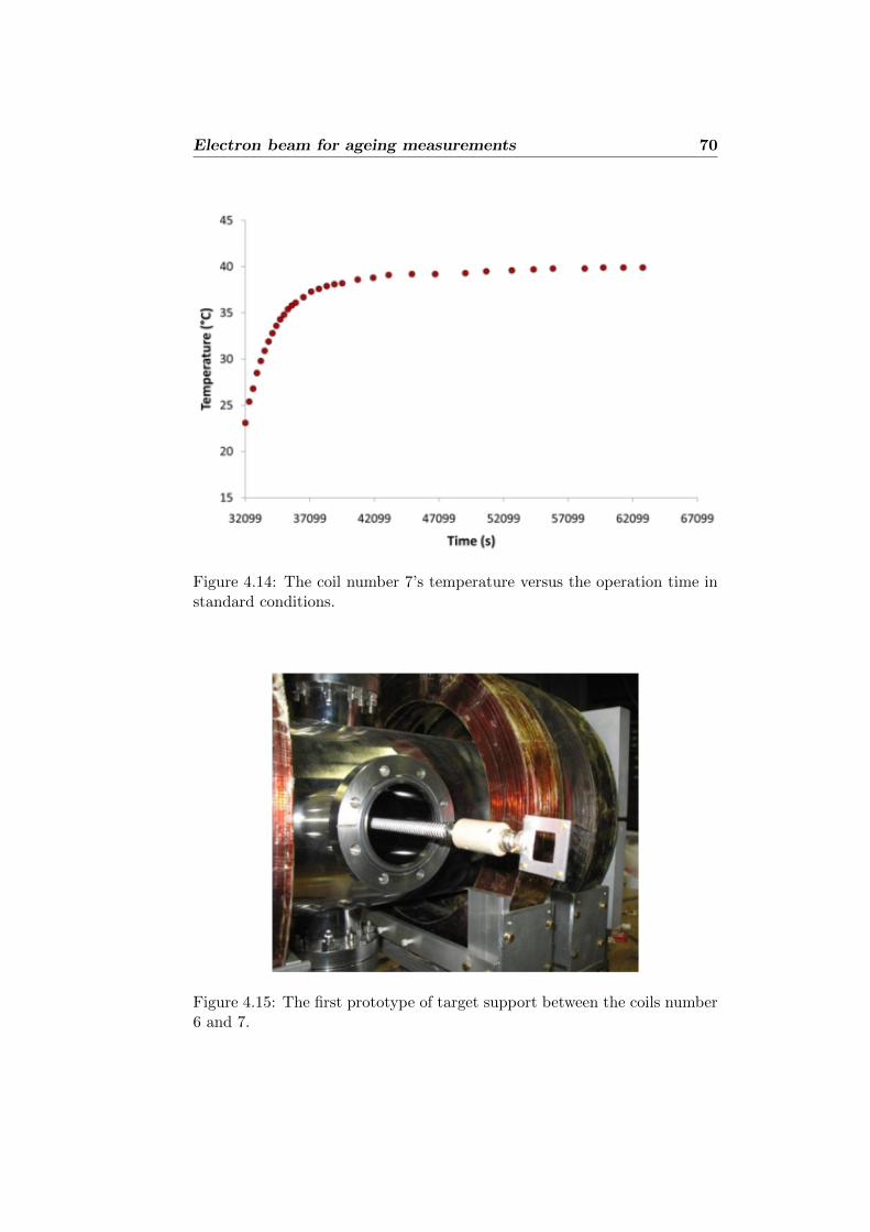
Electron beam for ageing measurements 70
Figure 4.14: The coil number 7’s temperature versus the operation time instandard conditions.
Figure 4.15: The first prototype of target support between the coils number6 and 7.
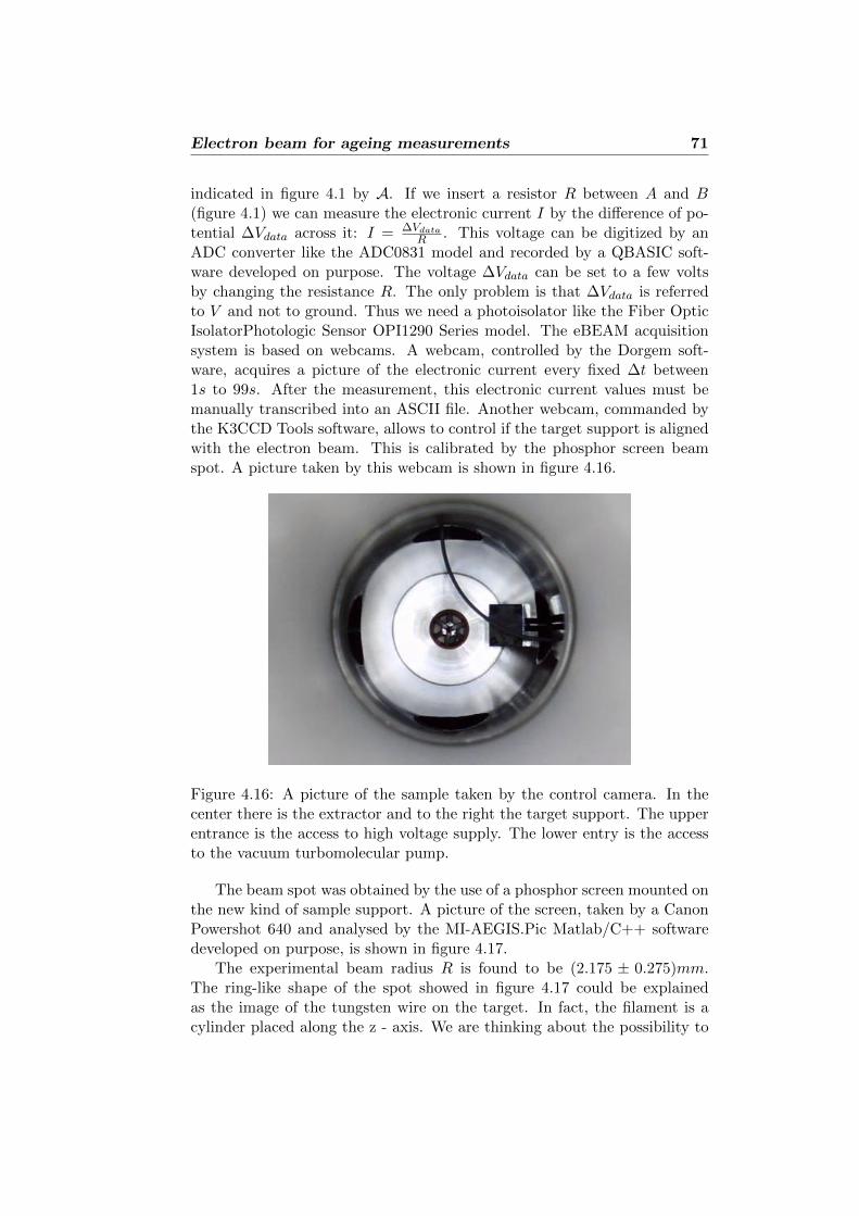
Electron beam for ageing measurements 71
indicated in figure 4.1 by A. If we insert a resistor R between A and B(figure 4.1) we can measure the electronic current I by the difference of po-tential ∆Vdata across it: I = ∆Vdata
R . This voltage can be digitized by anADC converter like the ADC0831 model and recorded by a QBASIC soft-ware developed on purpose. The voltage ∆Vdata can be set to a few voltsby changing the resistance R. The only problem is that ∆Vdata is referredto V and not to ground. Thus we need a photoisolator like the Fiber OpticIsolatorPhotologic Sensor OPI1290 Series model. The eBEAM acquisitionsystem is based on webcams. A webcam, controlled by the Dorgem soft-ware, acquires a picture of the electronic current every fixed ∆t between1s to 99s. After the measurement, this electronic current values must bemanually transcribed into an ASCII file. Another webcam, commanded bythe K3CCD Tools software, allows to control if the target support is alignedwith the electron beam. This is calibrated by the phosphor screen beamspot. A picture taken by this webcam is shown in figure 4.16.
Figure 4.16: A picture of the sample taken by the control camera. In thecenter there is the extractor and to the right the target support. The upperentrance is the access to high voltage supply. The lower entry is the accessto the vacuum turbomolecular pump.
The beam spot was obtained by the use of a phosphor screen mounted onthe new kind of sample support. A picture of the screen, taken by a CanonPowershot 640 and analysed by the MI-AEGIS.Pic Matlab/C++ softwaredeveloped on purpose, is shown in figure 4.17.
The experimental beam radius R is found to be (2.175 ± 0.275)mm.The ring-like shape of the spot showed in figure 4.17 could be explainedas the image of the tungsten wire on the target. In fact, the filament is acylinder placed along the z - axis. We are thinking about the possibility to
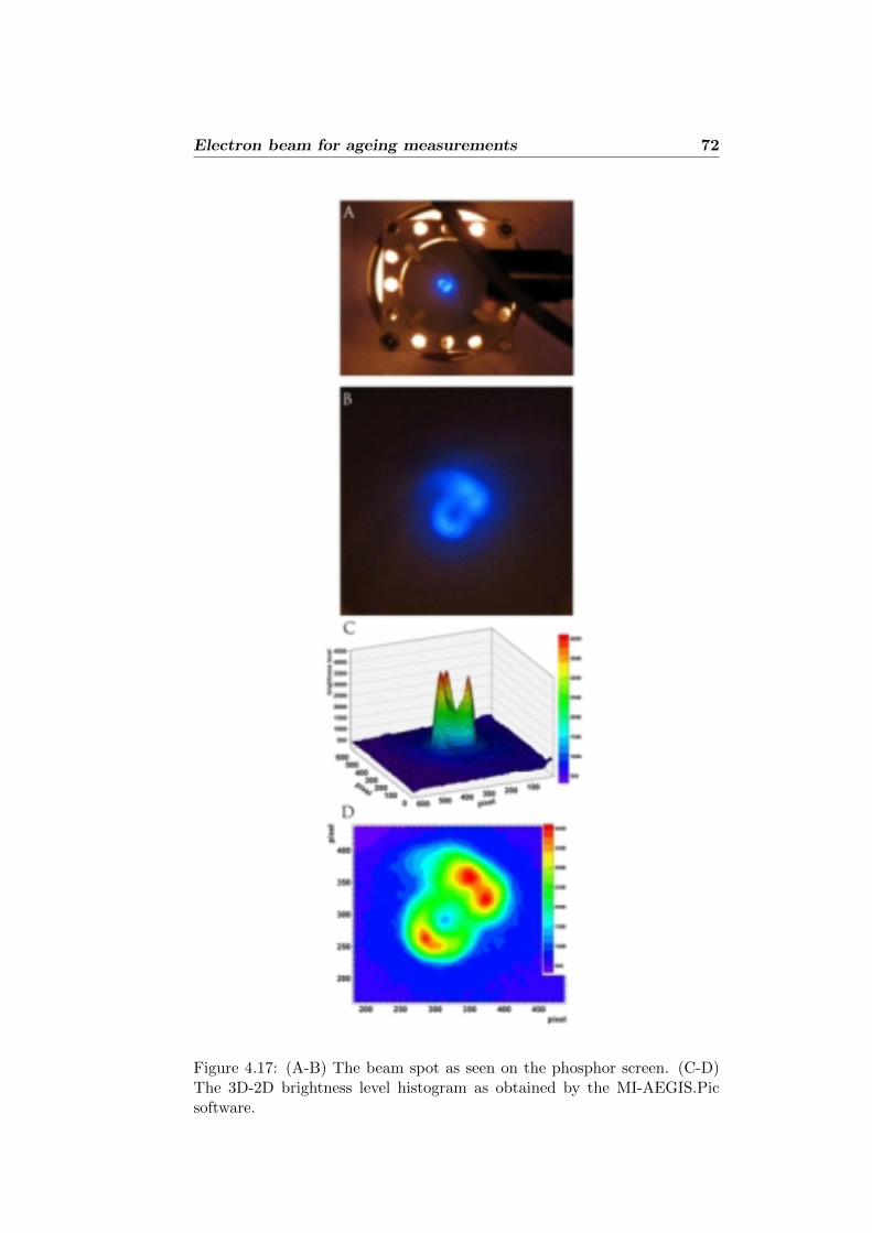
Electron beam for ageing measurements 72
Figure 4.17: (A-B) The beam spot as seen on the phosphor screen. (C-D)The 3D-2D brightness level histogram as obtained by the MI-AEGIS.Picsoftware.
Electron beam for ageing measurements 73
make an antenna measurements of the beam spot radius R versus the axialcoordinate z. In fact, an electron in cyclotron motion emits radiation withdiscrete frequencies. The more intense of them is the cyclotron frequency
(first harmonic) ωc = eBme
. Given that R =√
2Kmeω2
cand that the axial
magnetic field Bz is not uniform, but weakly depends on the axial coordinate
z, it is possible to determine the function R (z) =√
2Kmeω2
c (z)by measuring
the radiation frequency ωc (z). Given that R is a function of Bz it is also
possible to measure the axial magnetic field Bz (z) = meωc(z)e . This indirect
measure should be in agreement with the direct ones described in appendixB.
4.6 Ageing measurements
At the present status, we have built and characterized the electron beameBEAM. Given that electrons and positrons release the same amount ofenergy in solids, eBEAM can be used for ageing measurements of the AEgISconverter. In the near future, for each converter, we will able to measurethe positronium formation yield before and after irradiation by eBEAM.The converter radiation dose must be the same of which achieved in theAEgIS apparatus at CERN. Any change in the positronium formation yieldwill show the existence of a converter lifetime that it will be measured witheBEAM too.
Chapter 5
Conclusions
This PhD thesis is focused on the AEgIS antimatter experiment. The mainwork consisted in the design, realization and characterization of an electronbeam that can deliver up to 200µA with a tunable energy from 1 to 10keV .The system is immersed in a magnetic field and delivers a beam spot of(2.175± 0.275)mm radius. This machine, now fully operational, will beused for ageing measurements of positron to positronium converters for theAEgIS experiment. It has been demonstrated that many quantities like thepositronium formation yield or its outgoing velocity depend on the charac-teristics of the converter considered. In order to have the same conditionsthroughout the operating time of AEgIS , it is necessary to study the effectof positron radiation dose on the converter itself. Positrons and electronsbehave in the same way for what concern energy release in solids. The onlydifference is due to the annihilation gammas that anyway leave the AEgISconverters without depositing their energy. Thus we can make ageing mea-surements by using electrons instead of positrons. This choice has manyadvantages:
• obtaining an electron beam is simpler than obtaining a positron beam;
• the current of an electron beam is much grater than that of a positronbeam;
• an electron beam does not produce annihilation gamma rays.
In addition, I have been working on the design of the final AEgIS positronsource and participating in the studies and modelling needed for the choiceof the appropriate converter for the experiment.
Finally, I made measurements of positronium formation in liquid scin-tillators, of interest for solar neutrino detectors. Electron antineutrinos arecommonly detected in liquid scintillator experiments by inverse beta de-cay, looking at the coincidence between the reaction products, neutron andpositron. Prior to positron annihilation, an electron-positron pair may form
74

Conclusions 75
orthopositronium (o-Ps) with 50% probability. Even if the o-Ps decay isspeeded up by spin flip or pick up effects, its effective mean life is τ = 3ns.Such a mean life may introduce distorting effects in the photoelectron timedistribution, fundamental for position reconstruction and pulse shape dis-crimination algorithms in antineutrino experiments.
I would like to thank: Dr. M. G. Giammarchi and Prof. G. Consolati fortheir help during all my PhD activity; Dr. D. Franco for the PALS analysis;the AEgIS collaboration and in particular the L-NESS laboratory for thepossibility to collaborate with an international laboratory like CERN.

Appendix A
Thermionic emission fromtungsten wire
A.1 Introduction
In order to study the electron emission from an heated Tungsten wire (thermioniceffect), we consider the electrons in the metal to be in thermal equilibriumwith a dilute gas of electrons moving outside it. At temperature T theelectronic distribution function Ni (En) inside the metal is:
Ni(En) =1
eEn−µkBT + 1
, (A.1)
where the total energy En is determined by the band structure. kB is theBoltzmann constant and µ is the chemical potential. The electronic chargedistribution in primitive Wigner-Seitz cells of the metal near the surfacedoes not have the symmetry of the Bravais lattice so that such cells will,in general, have a non-vanishing electric dipole moment and may even yielda non-vanishing net electrical surface charge (figure A.1). The particularway in which the charge distribution in cells near the surface differs fromthat in the bulk depends on such details as whether the surface is planeor rough, and, if plane, on the orientation of the plane with respect to thecrystallographic axis. We first consider the case in which the distortion ofthe surface primitive cell does not result in a net macroscopic charge perunit area of metallic surface. However, within the surface layer in whichthe cells are distorted, this distortion will give rise to appreciable electricfields, against which the amount of work WS =
∫e ~E · ~dl must be performed,
in moving an electron through the layer. The work WS bring about a newdefinition of the metal work function1 W that, with reference to figure A.1,
1The metal work function is the energy that must be supplied to remove an electronfrom a metal.
76

Thermionic emission from tungsten wire 77
Figure A.1: Metallic solid structure.
is defined by:W = −EF +WS = −EF + eφ. (A.2)
The total energy E of an electron outside the metal should be taken tohave the free particle from
E = K + U = K + eφ, (A.3)
where K is the kinetic energy, U the electrostatic potential energy and φ isthe local value of the electrostatic potential seen before. At temperature Tthe electronic distribution function N0(E) outside the metal is:
N0(E) =1
eE−µ′kBT + 1
=1
eK+eφ−µ′kBT + 1
= N0(K), (A.4)
where µ′ is the chemical potential of the outer electron gas. Since the elec-tron gas inside the metal is in thermal equilibrium with electron gas outside,the chemical potential is the same, so that µ′ = µ. Moreover, inside themetal, at temperature below several thousand degrees, the chemical poten-tial differs negligibly from the Fermi energy so that µ ∼= EF .
N0(K) =1
eK+eφ−µ′kBT + 1
=1
eK+eφ−µkBT + 1
=1
eK−EF+eφ
kBT + 1
=1
eK−WkBT + 1
,
(A.5)Since work functions W are typically a few eV in size, W/kB is of the order104K. Therefore in the high temperature approximation N0(K) reduces to:
N0(K) = e−K−W
kBT . (A.6)

Thermionic emission from tungsten wire 78
From which it follows that at high temperature the electronic distributionfunction of the thermionic emitted electrons in vacuum (without externalpotentials) is given by a Maxwell - Boltzmann distribution.
A.2 The energy spectrum of the thermionicallyemitted electrons
The probability that a thermionic electron has a kinetic energy between Eand E + dE (energy spectrum) is given by:
P (E) d (E) =N0 (E)
Zg (E)V dE , (A.7)
where g (E)V dE is the density of states per unit volume (DOS) in the energyrange [E , E + dE ] by the volume V , i.e. the number of states between E andE + dE in the volume V . Moreover N0(E) is the electronic distributionfunction, i.e. the probability that one of these states is filled, and Z is thepartition function. Since
∫ +∞0 P (E)dE = 1 the partition function is:
Z = V
∫ +∞
0g (E)N0 (E) dE . (A.8)
The DOS for electrons in three dimensions is given by2:
g (E) =1
2π2
(2m
h
) 32
E12 , (A.9)
where m is the electron mass and h the reduced Plank constant. So, the par-tition function, given the electronic distribution function N0 (E), is describedby:
Z = V
∫ +∞
0g (E)N0 (E) dE
= V
∫ +∞
0
1
2π2
(2m
h
) 32
E12 e−K−W
kBT dE
=V
2π2
(2m
h
) 32
eWkBT
∫ +∞
0E
12 e− EkBT dE
=V
2π2
(2m
h
) 32
eWkBT
π12
2(kBT )
32
=V π
12
4π2
(2mkBT
h
) 32
eWkBT . (A.10)
2We had used a trick that is common in quantum mechanics: assume that the electronis in a large box (energy quantization) with zero potential energy (i.e. total energy is onlykinetic). At the end of calculation, we will allow the size of the box to became infinite,so that the separation levels tends to zero. For any macroscopic box side L, the energylevels are very close to each other and the continuous description works well.
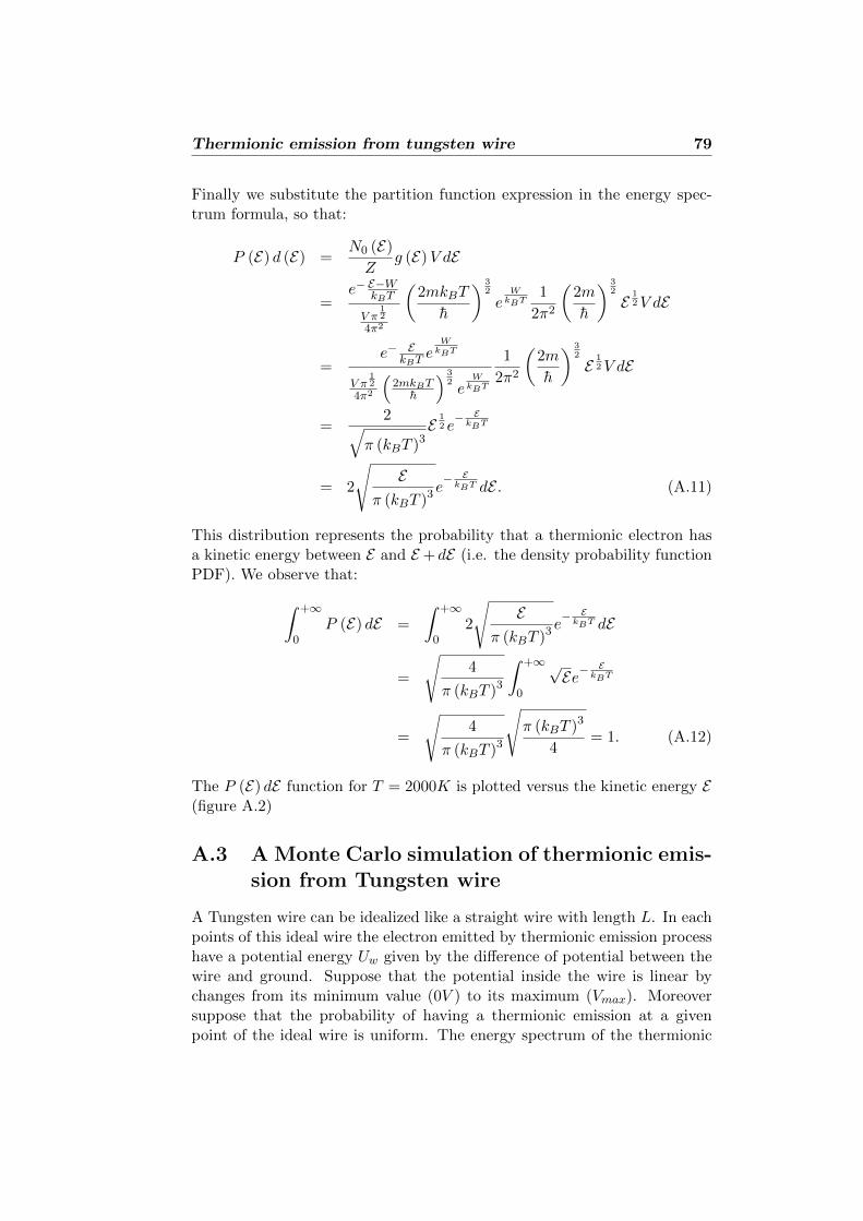
Thermionic emission from tungsten wire 79
Finally we substitute the partition function expression in the energy spec-trum formula, so that:
P (E) d (E) =N0 (E)
Zg (E)V dE
=e− E−WkBT
V π12
4π2
(2mkBT
h
) 32
eWkBT
1
2π2
(2m
h
) 32
E12V dE
=e− E
kBTe
WkBT
V π12
4π2
(2mkBT
h
) 32e
WkBT
1
2π2
(2m
h
) 32
E12V dE
=2√
π (kBT )3E
12 e− EkBT
= 2
√E
π (kBT )3 e− EkBT dE . (A.11)
This distribution represents the probability that a thermionic electron hasa kinetic energy between E and E + dE (i.e. the density probability functionPDF). We observe that:∫ +∞
0P (E) dE =
∫ +∞
02
√E
π (kBT )3 e− EkBT dE
=
√4
π (kBT )3
∫ +∞
0
√Ee−
EkBT
=
√4
π (kBT )3
√π (kBT )3
4= 1. (A.12)
The P (E) dE function for T = 2000K is plotted versus the kinetic energy E(figure A.2)
A.3 A Monte Carlo simulation of thermionic emis-sion from Tungsten wire
A Tungsten wire can be idealized like a straight wire with length L. In eachpoints of this ideal wire the electron emitted by thermionic emission processhave a potential energy Uw given by the difference of potential between thewire and ground. Suppose that the potential inside the wire is linear bychanges from its minimum value (0V ) to its maximum (Vmax). Moreoversuppose that the probability of having a thermionic emission at a givenpoint of the ideal wire is uniform. The energy spectrum of the thermionic
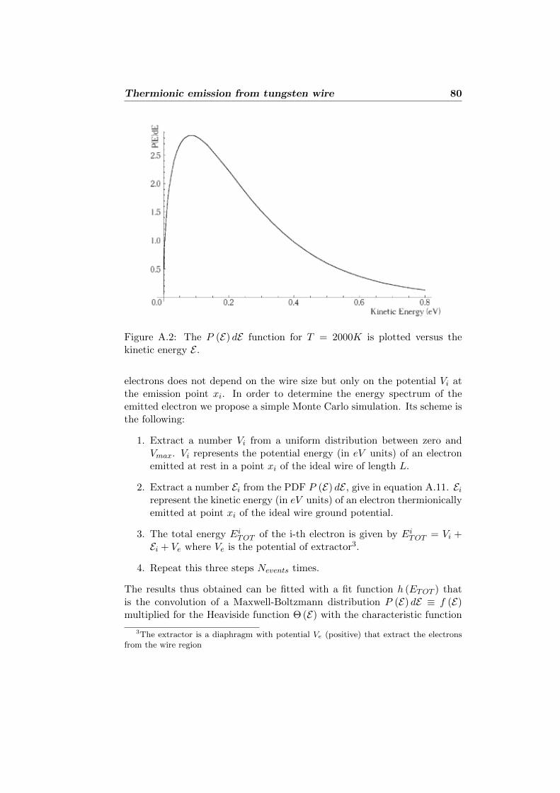
Thermionic emission from tungsten wire 80
Figure A.2: The P (E) dE function for T = 2000K is plotted versus thekinetic energy E .
electrons does not depend on the wire size but only on the potential Vi atthe emission point xi. In order to determine the energy spectrum of theemitted electron we propose a simple Monte Carlo simulation. Its scheme isthe following:
1. Extract a number Vi from a uniform distribution between zero andVmax. Vi represents the potential energy (in eV units) of an electronemitted at rest in a point xi of the ideal wire of length L.
2. Extract a number Ei from the PDF P (E) dE , give in equation A.11. Eirepresent the kinetic energy (in eV units) of an electron thermionicallyemitted at point xi of the ideal wire ground potential.
3. The total energy EiTOT of the i-th electron is given by EiTOT = Vi +Ei + Ve where Ve is the potential of extractor3.
4. Repeat this three steps Nevents times.
The results thus obtained can be fitted with a fit function h (ETOT ) thatis the convolution of a Maxwell-Boltzmann distribution P (E) dE ≡ f (E)multiplied for the Heaviside function Θ (E) with the characteristic function
3The extractor is a diaphragm with potential Ve (positive) that extract the electronsfrom the wire region
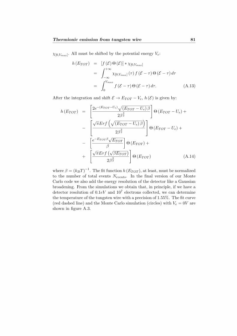
Thermionic emission from tungsten wire 81
χ[0,Vmax]. All must be shifted by the potential energy Ve:
h (ETOT ) = [f (E) Θ (E)] ∗ χ[0,Vmax]
=
∫ +∞
−∞χ[0,Vmax] (τ) f (E − τ) Θ (E − τ) dτ
=
∫ Vmax
0f (E − τ) Θ (E − τ) dτ. (A.13)
After the integration and shift E → ETOT − Ve, h (E) is given by:
h (ETOT ) =
[2e−(ETOT−Ue)
√(ETOT − Ue)β
2β32
]Θ (ETOT − Ue) +
−
√πErf(√
(ETOT − Ue)β)
2β32
Θ (ETOT − Ue) +
−[e−ETOT β
√ETOT
β
]Θ (ETOT ) +
+
[√πErf
(√βETOT
)2β
32
]Θ (ETOT ) (A.14)
where β = (kBT )−1. The fit function h (ETOT ), at least, must be normalizedto the number of total events Nevents. In the final version of our MonteCarlo code we also add the energy resolution of the detector like a Gaussianbroadening. From the simulations we obtain that, in principle, if we have adetector resolution of 0.1eV and 107 electrons collected, we can determinethe temperature of the tungsten wire with a precision of 1.55%. The fit curve(red dashed line) and the Monte Carlo simulation (circles) with Ve = 0V areshown in figure A.3.
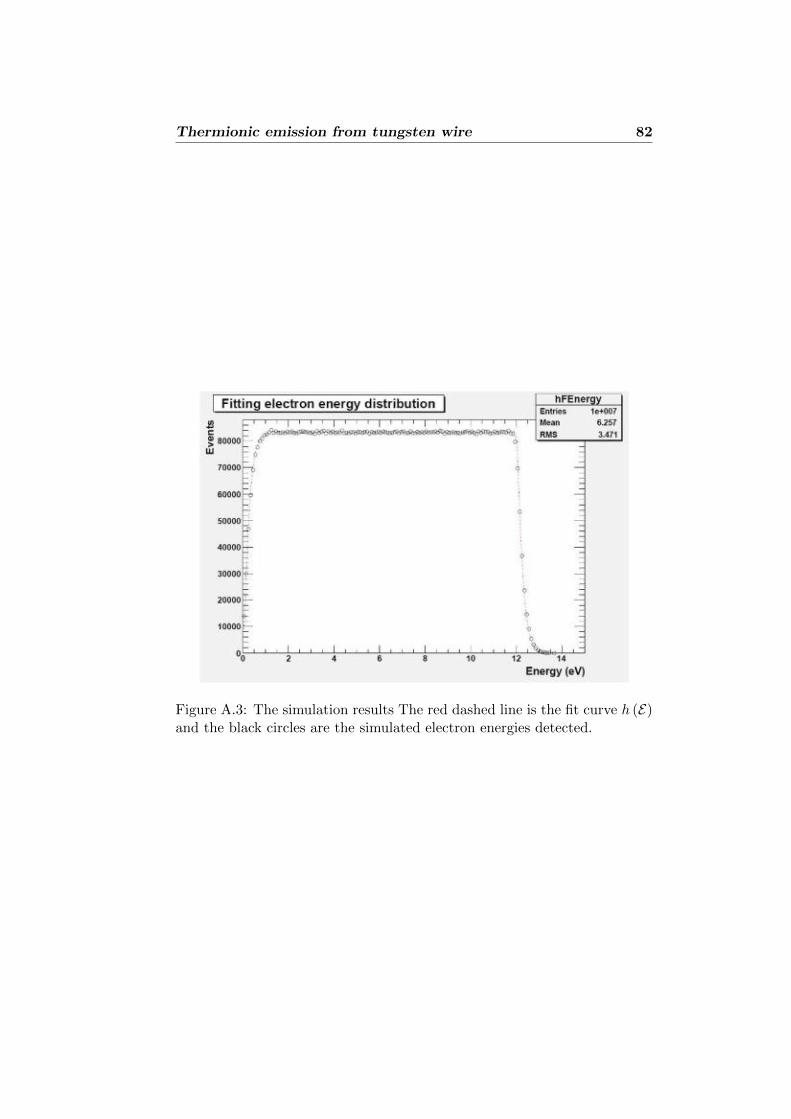
Thermionic emission from tungsten wire 82
Figure A.3: The simulation results The red dashed line is the fit curve h (E)and the black circles are the simulated electron energies detected.

Appendix B
The eBEAM magnetic field
B.1 Magnetic field calculation
B.1.1 Introduction
In this chapter we discuss the magnetic field generated by a finite solenoid(coil) [70]. In our theoretical discussion we will use cylindrical coordinatesin the half-space z ≥ 0 and model each coil by a cylindrical shell volumecurrent. The origin of cylindrical coordinates is taken at the axis of thecoil with z = 0 at its end. We will use Bessel functions in our calculationsalthough other functions, such as Legendre functions and polynomials, couldhave been used as well. A current loop C of infinitesimal radius ρ′, carryingcurrent I, is located to the plane xy with center on the z axis (see figureB.1).
Figure B.1: The geometry of the cylindrical shell volume current used inthis section. a is the inner radius b the outer and L the thickness of thecylinder.
83
The eBEAM magnetic field 84
The vector potential of the loop is
~A (~x) =µ0I
4π
∮Cd
d~l′
|~x− ~x′|, (B.1)
where µ0 is the permeability of free space and d~l′ = ρ′dφ′eφ. The unitvector eφ is oriented in the positive sense of the polar angle φ. The integralin equation B.1 can be calculated by a series expansion of |~x−~x′|−1 in termsof the Bessel functions Jm (ξ):
1
|~x− ~x′|=
+∞∑m=−∞
∫ +∞
0dkeim(φ−φ′)Jm (kρ) Jm
(kρ′)e−k|z−z
′|. (B.2)
The magnitude of the vector potential is independent of φ because of theazimuthal symmetry of the currents. After integration with respect to φ′,only terms with indices m = −1, 1 remain in the sum. By using the identityJ−1 (ξ) = −J1 (ξ), the x component of the potential vanishes and the vectorpotential becomes
~A (ρ, z) =µ0Iρ
′
2ey
∫ +∞
0dkJ1 (kρ) J1
(kρ′)e−k|z−z
′|. (B.3)
Equation B.3 is obtained for φ = 0 with ey = eφ. Another choice of φ wouldnot change the potential. If we take into account that the vector potentialhas the same direction as the current, we can let ~A = Aφeφ where
Aφ (ρ, z) =µ0Iρ
′
2
∫ +∞
0dkJ1 (kρ) J1
(kρ′)e−k|z−z
′|. (B.4)
By use of this last equation and the superposition principle, we can derive thevector potential of an arbiter cylindrically symmetric current distribution.The finite coil can be modeled by a cylindrical shell current ~K = Keφ with:
K =∆I
∆S′=
NI
(b− a)L(B.5)
where N is the number of turns of the coil and ∆S′ = ∆ρ′∆z′ is the finitesurface element. We use the equation B.4 for a narrow ∆z′ and ∆ρ′ stripcarrying the current ∆I and obtain
∆Aφ (ρ, z) =µ0∆Iρ′
2
∫ +∞
0dkJ1 (kρ) J1
(kρ′)e−k|z−z
′|. (B.6)
Now, using the superposition principle we obtain the vector potential of theentire cylinder in the limit ∆z′ → 0 and ∆ρ′ → 0,
Aφ (ρ, z) =µ0NI
2 (b− a)L
∫ L
0dz′∫ b
adρ′ρ′
∫ +∞
0dkJ1 (kρ) J1
(kρ′)e−k|z−z
′|
(B.7)
The eBEAM magnetic field 85
After integration with respect to z′ and ρ′ the vector potential becomes
Aφ (ρ, z) =µ0NIa
2π
4L (b− a)
∫ +∞
0dkJ1 (kρ)
kf (k; z) g (k) . (B.8)
where the function f (k; z) is defined by:
f (k; z) =
e−k(z−L) − e−kz, z ≥ L2− e−k(L−z) − e−kz, 0 ≤ z < L
. (B.9)
and g (k) is given by
g (k) =1
ka
[− J1 (ka)H0 (ka) +
b
aJ1 (kb)H0 (kb) + J0 (ka)H1 (ka) +
− b
aJ0 (kb)H1 (kb)
], (B.10)
where H0 (ζ) and H1 (ζ) are Struve functions 1. The magnetic field,corresponding to the potential ~A (ρ, z), is calculated using ~B (ρ, z) = ~∇ ×~A (ρ, z) in cylindrical coordinates:
~B (ρ, z) = −∂Aφ (ρ, z)
∂zeρ +
1
ρ
∂
∂ρ[ρAφ (ρ, z)] ez. (B.12)
So, we obtain:
Bρ (ρ, z) =µ0NI
L
a2π
4 (b− a)
∫ +∞
0dkJ1 (kρ)
[e−k|z−L| − e−kz
]g (k)
Bz (ρ, z) =µ0NI
L
a2π
4 (b− a)
∫ +∞
0dkJ0 (kρ) f (k; z) g (k) . (B.13)
These two integrals have to be done numerically to obtain the final valuesfor the magnetic field.
B.1.2 MI-AEGIS.Mag
Theoretically, the magnetic field generated by a finite solenoid is given bythe equations B.13. These equations do not have analytical solutions andmust be solved numerically for each point of space. In order to compute
1The Struve function Hn (ζ) are solutions of the non-homogeneous Bessel’s differentialequation and are defined as:
Hn (ζ) =
(1
2ζ
)n+1 +∞∑k=0
(−1)k(12ζ)2k
Γ(k + 3
2
)Γ(k + n+ 3
2
) . (B.11)
The complex number n is the order of the Struve function, and in our studies is an integer.
The eBEAM magnetic field 86
the total magnetic field vector ~B (ρ, z) generated by a set of N coils, wedeveloped a C++ program, MI-AEGIS.Mag (version 3.5). The main inputsare the simulation space in cylindrical coordinates [ρMAX , zMAX ] and thespace resolution that is the number of points in which the program computethe magnetic field vector. The maximum number of coils (like the simulationspace) depends on the amount of computer memory available, in our caseis 112. For every coil, MI-AEGIS.Mag compute the magnetic field vector~Bi (ρ, z) in each point of the simulation space. Moreover it is useful to usethe symmetry of the problem respect the coil axis plane z = 0. In fact, themagnetic field vector ~B (ρ0, z0) at a given point (ρ0, z0) is related with theone in (ρ0,−z0) by:
Bz (ρ0, z0) = Bz (ρ0,−z0) (B.14)
Bρ (ρ0, z0) = −Bρ (ρ0,−z0) . (B.15)
This symmetry reduces the computational time. In order to integrate theequations B.13 we developed a set o libraries and functions. We use theSimpson’s integration method that guarantees the best time to error ra-tio for our problem. We try also other integration methods like the gaussmethod, but we did not obtain better results. We find the number of Simp-son’s integration steps Nstep = 2700 by means of the study of the time toerror ratio and the integration range in k given by [0.001, 5000]m−1. Thealgorithm is stable up to 1mm in space resolution (for both ρ and z). Whenall the ~Bi (ρ, z) are computed, the total magnetic field vector ~BTOT (ρ, z) isgiven by:
~BTOT (ρ, z) =N∑i=1
~Bi (ρ, z) (B.16)
The output of the program are three files: Mag Rho.txt, Mag Zeta.txt andMag.txt. The first and the second ones represent the cylindrical componentsof the magnetic field vector ~BTOT (ρ, z). The last one is the absolute value| ~BTOT (ρ, z) | given by:
| ~BTOT (ρ, z) | =
√√√√[ N∑i=1
Bρ,i (ρ, z)
]2
+
[ N∑i=1
Bz,i (ρ, z)
]2
(B.17)
These files can be imported in CERN/ROOT in order to visualize the mag-netic field computed. The magnetic field ~BTOT (0, z) computed by MI-AEGIS.Mag was compared with the analytical approximation given by E.Dennison:
2Corresponding to a personal computer with 4Gb of memory
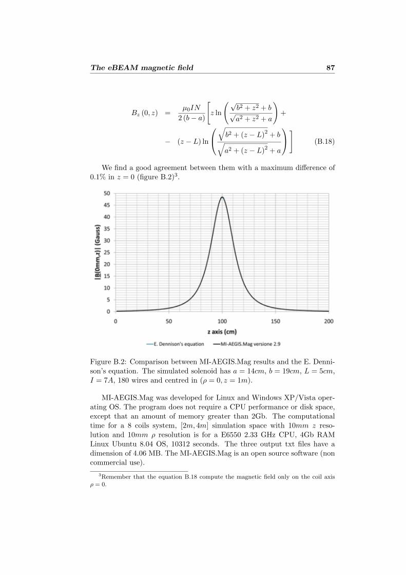
The eBEAM magnetic field 87
Bz (0, z) =µ0IN
2 (b− a)
[z ln
(√b2 + z2 + b√a2 + z2 + a
)+
− (z − L) ln
√b2 + (z − L)2 + b√a2 + (z − L)2 + a
] (B.18)
We find a good agreement between them with a maximum difference of0.1% in z = 0 (figure B.2)3.
Figure B.2: Comparison between MI-AEGIS.Mag results and the E. Denni-son’s equation. The simulated solenoid has a = 14cm, b = 19cm, L = 5cm,I = 7A, 180 wires and centred in (ρ = 0, z = 1m).
MI-AEGIS.Mag was developed for Linux and Windows XP/Vista oper-ating OS. The program does not require a CPU performance or disk space,except that an amount of memory greater than 2Gb. The computationaltime for a 8 coils system, [2m, 4m] simulation space with 10mm z reso-lution and 10mm ρ resolution is for a E6550 2.33 GHz CPU, 4Gb RAMLinux Ubuntu 8.04 OS, 10312 seconds. The three output txt files have adimension of 4.06 MB. The MI-AEGIS.Mag is an open source software (noncommercial use).
3Remember that the equation B.18 compute the magnetic field only on the coil axisρ = 0.
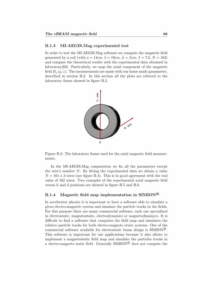
The eBEAM magnetic field 88
B.1.3 MI-AEGIS.Mag experimental test
In order to test the MI-AEGIS.Mag software we compute the magnetic fieldgenerated by a coil (with a = 14cm, b = 19cm, L = 5cm, I = 7A, N = 162)and compare the theoretical results with the experimental data obtained inlaboratory[69]. Particularly, we map the axial component of the magneticfieldBz (ρ, z). The measurements are made with our home made gaussmeter,described in section B.2. In this section all the plots are referred to thelaboratory frame showed in figure B.3.
Figure B.3: The laboratory frame used for the axial magnetic field measure-ments.
In the MI-AEGIS.Mag computation we fix all the parameters exceptthe wire’s number N . By fitting the experimental data we obtain a valueN = 161± 3 wires (see figure B.4). This is in good agreement with the realvalue of 162 wires. Two examples of the experimental axial magnetic fieldversus h and d positions are showed in figure B.5 and B.6.
B.1.4 Magnetic field map implementation in SIMION R©
In accelerator physics it is important to have a software able to simulate agiven electro-magnetic system and simulate the particle tracks in the fields.For this purpose there are many commercial software, each one specializedin electrostatic, magnetostatic, electrodynamics or magnetodinamycs. It isdifficult to find a software that computes the field map and simulates therelative particle tracks for both electro-magneto static systems. One of thecommercial software available for electrostatic beam design is SIMION R©.This software is important for our applications because it also allows toimplement a magnetostatic field map and simulate the particles tracks ina electro-magneto static field. Generally SIMION R© does not compute the
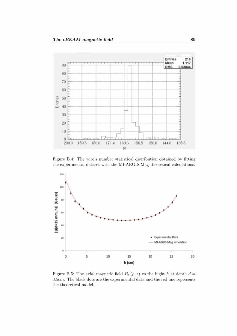
The eBEAM magnetic field 89
Figure B.4: The wire’s number statistical distribution obtained by fittingthe experimental dataset with the MI-AEGIS.Mag theoretical calculations.
Figure B.5: The axial magnetic field Bz (ρ, z) vs the hight h at depth d =3.5cm. The black dots are the experimental data and the red line representsthe theoretical model.
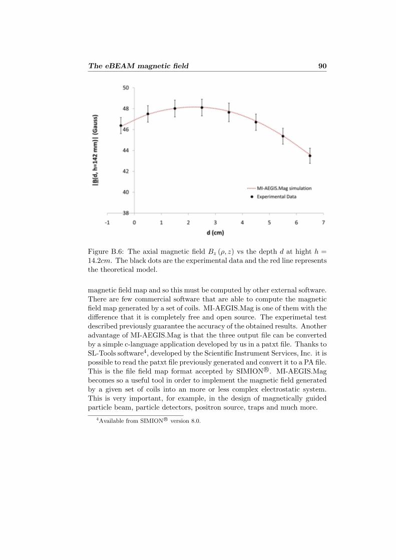
The eBEAM magnetic field 90
Figure B.6: The axial magnetic field Bz (ρ, z) vs the depth d at hight h =14.2cm. The black dots are the experimental data and the red line representsthe theoretical model.
magnetic field map and so this must be computed by other external software.There are few commercial software that are able to compute the magneticfield map generated by a set of coils. MI-AEGIS.Mag is one of them with thedifference that it is completely free and open source. The experimetal testdescribed previously guarantee the accuracy of the obtained results. Anotheradvantage of MI-AEGIS.Mag is that the three output file can be convertedby a simple c-language application developed by us in a patxt file. Thanks toSL-Tools software4, developed by the Scientific Instrument Services, Inc. it ispossible to read the patxt file previously generated and convert it to a PA file.This is the file field map format accepted by SIMION R©. MI-AEGIS.Magbecomes so a useful tool in order to implement the magnetic field generatedby a given set of coils into an more or less complex electrostatic system.This is very important, for example, in the design of magnetically guidedparticle beam, particle detectors, positron source, traps and much more.
4Available from SIMIONR© version 8.0.

The eBEAM magnetic field 91
B.2 A gaussmeter design for the eBEAM appara-tus.
We have designed, built and operated a low-cost gaussmeter for measuringmagnetic fields in the range [0, 670G]. It is made by two parts: the firstone is the Hall sensor producing a voltage proportional to the magnetic fieldintensity and the second one is the controller, an electronic circuit for thecalibration of the scale between the output voltage of the Hall sensor andthe magnetic field. In particular we set 1mV = 1G.
Figure B.7: A picture of the low-cost homemade gaussmeter.
The Hall sensor is the SS495A1, glued on a plexiglass backing in orderto measure axial fields. The electronic scheme of the controller is showed infigure B.8.
It is possible to calibrate the device through the two trimmer (20kΩ, 50kΩ)as shown in figureB.8. The linearity of the gaussmeter was tested using theaxial magnetic field generated by a coil in the (z = 0, ρ = 0) point. Theexperimental data are reported in figure B.9.
A picture of the apparatus is showed in figure B.7.
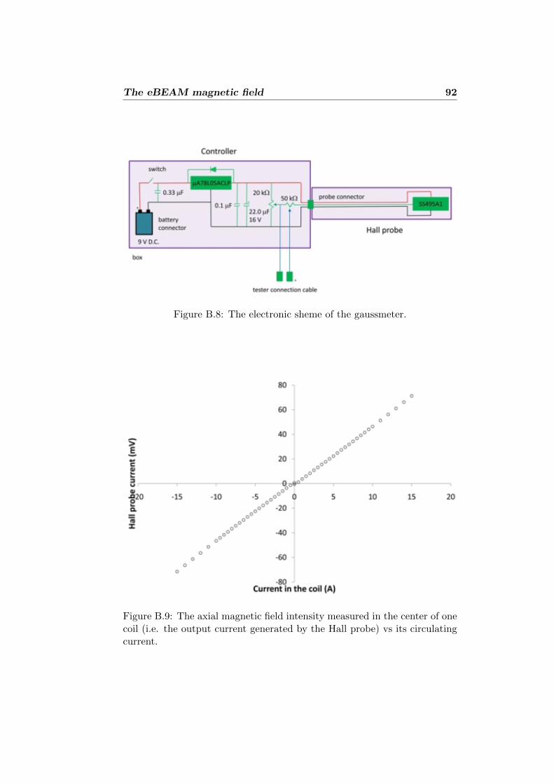
The eBEAM magnetic field 92
Figure B.8: The electronic sheme of the gaussmeter.
Figure B.9: The axial magnetic field intensity measured in the center of onecoil (i.e. the output current generated by the Hall probe) vs its circulatingcurrent.
Bibliography
[1] J. Scherk. Physics Letter, 88 B:265, 1979.
[2] G. Luders. Annals of Physics, 2:1, 1957.
[3] K. Nakamura et al. (Particle Data Group). Journal of Physics G,37:075021, 2010.
[4] A. Kellerbauer et al. (AEGIS Proto-collaboration). Nuclear Instru-ments and Measurements B, 266:351, 2008.
[5] G. Baur et al. Physics Letters B, 368:251, 1996.
[6] R. Klapisch. Physica Scripta, T5:140, 1983.
[7] J. B. Adams. Nature, 185:568, 1960.
[8] G. Blanford et al. Physical Review Letters, 80:3037, 1998.
[9] S. Baird et al. Nuclear Instruments and Methods in Physics ResearchA, 391:210, 1997.
[10] G. Gabrielse et al. Technical Report SPSC-P-306. CERN-SPSC-97-8,1997.
[11] M. H. Holzscheiter et al. Hyperfine interaction, 109:1, 1997.
[12] M. Amoretti et al. Nature, 419:456, 2002.
[13] G. Gabrielse et al. Physical Review Letters, 89:233401, 2002.
[14] W. Bertsche et al. AIP Conference Proceedings, 796:301, 2005.
[15] G. Drobychev et al. Technical Report SPSC-P-334. CERN-SPSC-2007-017, 2007.
[16] Yasunori Yamazaki. Nuclear Instruments and Methods in Physics Re-search Section B, 154:174, 1999.
[17] C. Maggiore et al. Nuclear Instruments and Methods in Physics Re-search Section B, 214:181, 2004.
93
BIBLIOGRAPHY 94
[18] G. Testera et al. AIP Conference Proceedings, 1037:5, 2008.
[19] I. Boscolo et al. Technical Report SPSC-SR-055. CERN-SPSC-2010-003, 2010.
[20] I. N. Meshkov et al. Instruments and Experimental Techniques, 50:639,2007.
[21] K. G. Lynn et al. Applied Physics Letters, 55:87, 1989.
[22] M. Kallenrode. Space Physics: An Introduction to Plasmas and Par-ticles in the Heliosphere and Magnetospheres. Springer; 3rd edition,2004.
[23] S. J. Gilbert. A New Ultra-Cold Positron Beam and Applications ToLow-Energy Positron Scattering and Electron-Positron Plasmas. PhDThesis, 2000.
[24] A. Rich. Review of Modern Physics, 53:127, 1981.
[25] J. A. Wheeler. Annalen New York Accademy Science, 48:219, 1946.
[26] A. Ore and J. L. Powell. Physical Review, 75:1696, 1949.
[27] R. Ley and G. With. Positronium: Theory versus experiment in Hy-drogen Atom. Springer-Verlag, Heidelberg, 2002.
[28] P.J. Schultz and K. G. Lynn. Review of Modern Physics, 60:701, 1988.
[29] R. Ley et al. Journal of Physics B: Atomic, Molecular and OpticalPhysics, 23:3437, 1990.
[30] F. Castelli et al. Physical Review A, 78:052512, 2008.
[31] M. Charlton and J. W. Humberston. Positron Physics. CambridgeUniversity Press, 2000.
[32] W. Brandt and A. Dupasquier. Proceedinds International School ofPhysics ”Enrico Fermi” Varenna on Lake Como, Course LXXXIII.North-Holland, Amsterdam, 1983.
[33] A. Ore. Arbok University of Bergen, (9), 1949.
[34] O. E. Mogensen. Journal of Chemistry Physics, 60:598, 1974.
[35] D. Trezzi. Studio della produzione di Positronio nell’esperimentoAEGIS. Master Thesis, 2006-2007.
[36] M. Dapor. Electron-Beam Interactions with Solids. Springer, 2003.
BIBLIOGRAPHY 95
[37] J. M. Fernandez Varea et al. Nuclear Instruments and Methods inPhysics B, 108:35, 1996.
[38] G. F. Knoll. Radiation Detection and Measurement. Wiley; 3rd edition,2000.
[39] H. Gumus et al. Chinese Journal of Physics, 44:290, 2006.
[40] K.A. Ritley et al. Journal of Applied Physics, 74:3479, 1993.
[41] S. Van Petegem et al. Physical Review B, 70:115410, 2004.
[42] M. Dapor. Journal of Electron Spectroscopy and Related Phenomena,151:182, 2006.
[43] P. Sferlazzo et al. Physical Review B, 35:5315, 1987.
[44] R. S. Vallery et al. Physical Review Letters, 90:203402, 2003.
[45] D. W. Gidley et al. Physical Review Letters, 36:395, 1976.
[46] S. J. Tao. Journal of Physics Chemistry, 56:5499, 1972.
[47] I. K. MacKenzie. Experimental Methods of Annihilation Time and En-ergy Spectrometry in Positron Solid-State Physics. Eds, North-Holland,Amsterdam, 1983.
[48] D. M. Shrader and Y. C. Jean. Positron and Positronium Chemistry.Eds, Elsevier, Amsterdam, 1988.
[49] H. Saito et al. Nuclear Instruments and Methods in Physics ResearchA, 487:612, 2002.
[50] K. Rytsola et al. Applied Surface Science, 194:260, 2002.
[51] F. Becvar. Nuclear Instrument Methods Physics for Research B,261:871, 2007.
[52] P. Kirkegaard and M. Eldrup. Computational Physics Communications,3:240, 1972.
[53] R.B. Gregory. Nuclear Instrument Methods for Physics Research A,302:496, 1991.
[54] A. Shukla et al. Nuclear Instrument Methods for Physics Research A,335:310, 1993.
[55] J. Kansy. Nuclear Instrument Methods for Physics Research A, 374:235,1996.
[56] G. Alimonti et al. Nuclear Instruments and Methods A, 600:568, 2009.
BIBLIOGRAPHY 96
[57] T. Mitsui and KamLAND collaboration. Nuclear Physics B - Proceed-ings Supplements, 117:13, 2003.
[58] I. Antcheva et al. Computer Physics Communications, 180:2499, 2009.
[59] H. O. Back et al. Nuclear Instruments and Methods A, 584:98, 2008.
[60] T. Marrodn Undagoitia et al. Review of Scientific Instruments,80:043301, 2009.
[61] S. Marder et al. Physical Review, 103:1258, 1956.
[62] R. Ferragut et al. Journal of Physics: Conference Series, 225:012007,2010.
[63] M. Baiguera. Sintesi e caratterizzazione di sospensioni di silice col-loidale. Bachelor Thesis, 2007-2008.
[64] N. Djourelov et al. Journal of Physics: Condensed Matter, 20:095206,2008.
[65] S. S. Kistler. Nature, 127 (3211):741, 1931.
[66] S. Mariazzi et al. Physical Review B, 81:235418, 2010.
[67] S. Mariazzi et al. Physical Review Letters, 104:243401, 2010.
[68] M. Eldrup et al. Physical Review B, 32:7048, 1985.
[69] A. Palman. Caratterizzazione di un sistema magnetico per una guidadi campo magnetico di fasci elettronici. Bachelor Thesis, 2007-2008.
[70] V. Labinac et al. American Journal of Physics, 74:521, 2006.
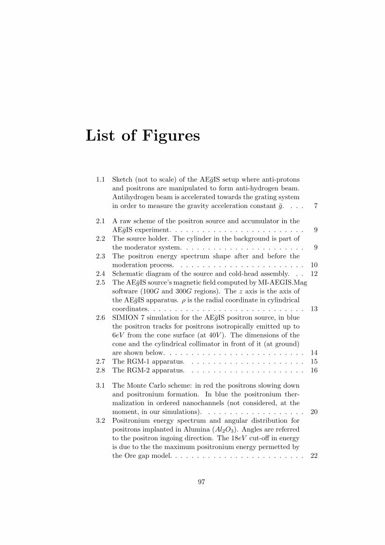
List of Figures
1.1 Sketch (not to scale) of the AEgIS setup where anti-protonsand positrons are manipulated to form anti-hydrogen beam.Antihydrogen beam is accelerated towards the grating systemin order to measure the gravity acceleration constant g. . . . 7
2.1 A raw scheme of the positron source and accumulator in theAEgIS experiment. . . . . . . . . . . . . . . . . . . . . . . . . 9
2.2 The source holder. The cylinder in the background is part ofthe moderator system. . . . . . . . . . . . . . . . . . . . . . . 9
2.3 The positron energy spectrum shape after and before themoderation process. . . . . . . . . . . . . . . . . . . . . . . . 10
2.4 Schematic diagram of the source and cold-head assembly. . . 122.5 The AEgIS source’s magnetic field computed by MI-AEGIS.Mag
software (100G and 300G regions). The z axis is the axis ofthe AEgIS apparatus. ρ is the radial coordinate in cylindricalcoordinates. . . . . . . . . . . . . . . . . . . . . . . . . . . . . 13
2.6 SIMION 7 simulation for the AEgIS positron source, in bluethe positron tracks for positrons isotropically emitted up to6eV from the cone surface (at 40V ). The dimensions of thecone and the cylindrical collimator in front of it (at ground)are shown below. . . . . . . . . . . . . . . . . . . . . . . . . . 14
2.7 The RGM-1 apparatus. . . . . . . . . . . . . . . . . . . . . . 152.8 The RGM-2 apparatus. . . . . . . . . . . . . . . . . . . . . . 16
3.1 The Monte Carlo scheme: in red the positrons slowing downand positronium formation. In blue the positronium ther-malization in ordered nanochannels (not considered, at themoment, in our simulations). . . . . . . . . . . . . . . . . . . 20
3.2 Positronium energy spectrum and angular distribution forpositrons implanted in Alumina (Al2O3). Angles are referredto the positron ingoing direction. The 18eV cut-off in energyis due to the the maximum positronium energy permetted bythe Ore gap model. . . . . . . . . . . . . . . . . . . . . . . . . 22
97
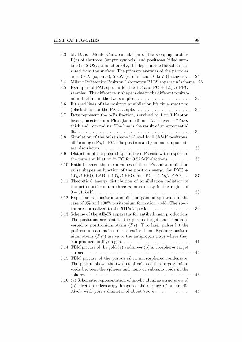
LIST OF FIGURES 98
3.3 M. Dapor Monte Carlo calculation of the stopping profilesP(z) of electrons (empty symbols) and positrons (filled sym-bols) in SiO2 as a function of z, the depth inside the solid mea-sured from the surface. The primary energies of the particlesare: 3 keV (squares), 5 keV (circles) and 10 keV (triangles). . 24
3.4 Milano Politecnico Positron Laboratory PALS apparatus’ scheme. 283.5 Examples of PAL spectra for the PC and PC + 1.5g/l PPO
samples. The difference in shape is due to the different positro-nium lifetime in the two samples. . . . . . . . . . . . . . . . . 32
3.6 Fit (red line) of the positron annihilation life time spectrum(black dots) for the PXE sample. . . . . . . . . . . . . . . . . 33
3.7 Dots represent the o-Ps fraction, survived to 1 to 3 Kaptonlayers, inserted in a Plexiglas medium. Each layer is 7.5µmthick and 1cm radius. The line is the result of an exponentialfit. . . . . . . . . . . . . . . . . . . . . . . . . . . . . . . . . . 34
3.8 Simulation of the pulse shape induced by 0.5MeV positrons,all forming o-Ps, in PC. The positron and gamma componentsare also shown. . . . . . . . . . . . . . . . . . . . . . . . . . . 36
3.9 Distortion of the pulse shape in the o-Ps case with respect tothe pure annihilation in PC for 0.5MeV electrons. . . . . . . 36
3.10 Ratio between the mean values of the o-Ps and annihilationpulse shapes as function of the positron energy for PXE +1.0g/l PPO, LAB + 1.0g/l PPO, and PC + 1.5g/l PPO. . . 37
3.11 Theoretical energy distribution of annihilation radiation ofthe ortho-positronium three gamma decay in the region of0− 511keV . . . . . . . . . . . . . . . . . . . . . . . . . . . . . 38
3.12 Experimental positron annihilation gamma spectrum in thecase of 0% and 100% positronium formation yield. The spec-tra are normalized to the 511keV peak. . . . . . . . . . . . . 39
3.13 Scheme of the AEgIS apparatus for antihydrogen production.The positrons are sent to the porous target and then con-verted to positronium atoms (Ps). Two laser pulses hit thepositronium atoms in order to excite them. Rydberg positro-nium atoms (Ps∗) arrive to the antiproton traps where theycan produce antihydrogen. . . . . . . . . . . . . . . . . . . . . 41
3.14 TEM picture of the gold (a) and silver (b) microspheres targetsurface. . . . . . . . . . . . . . . . . . . . . . . . . . . . . . . 42
3.15 TEM picture of the porous silica microspheres condensate.The picture shows the two set of voids of this target: microvoids between the spheres and nano or subnano voids in thespheres. . . . . . . . . . . . . . . . . . . . . . . . . . . . . . . 43
3.16 (a) Schematic representation of anodic alumina structure and(b) electron microscopy image of the surface of an anodicAl2O3 with pore’s diameter of about 70nm. . . . . . . . . . . 44
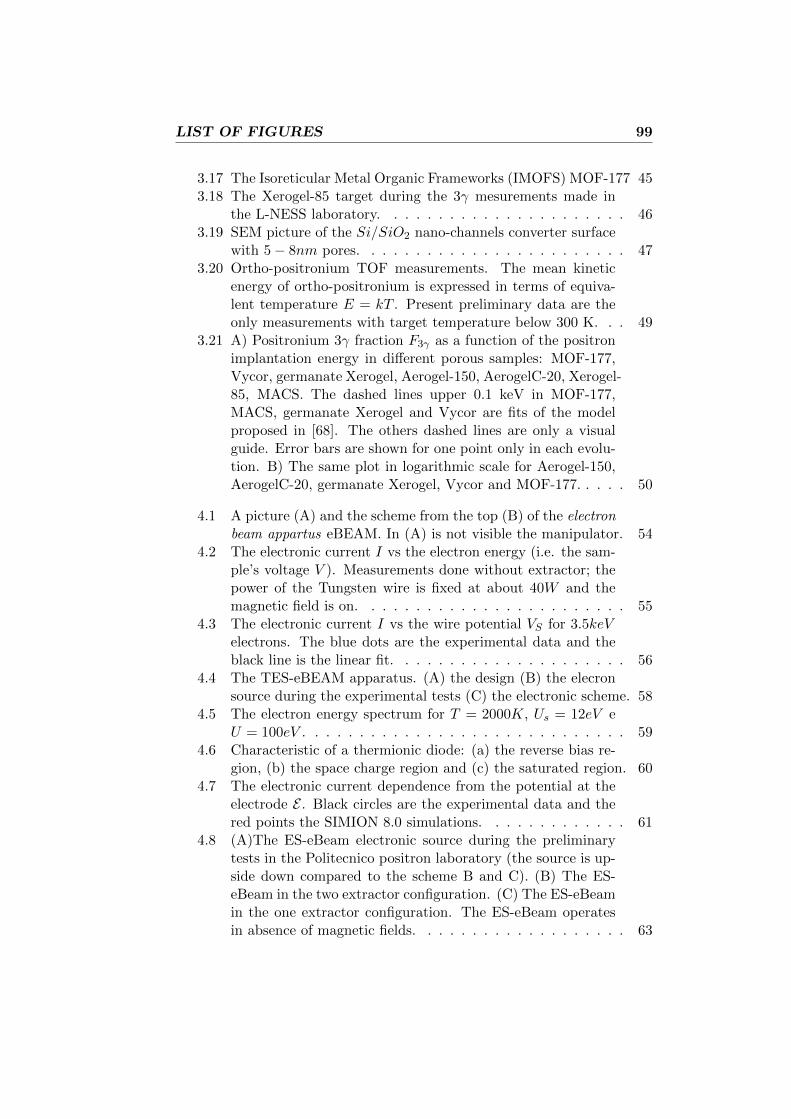
LIST OF FIGURES 99
3.17 The Isoreticular Metal Organic Frameworks (IMOFS) MOF-177 453.18 The Xerogel-85 target during the 3γ mesurements made in
the L-NESS laboratory. . . . . . . . . . . . . . . . . . . . . . 463.19 SEM picture of the Si/SiO2 nano-channels converter surface
with 5− 8nm pores. . . . . . . . . . . . . . . . . . . . . . . . 473.20 Ortho-positronium TOF measurements. The mean kinetic
energy of ortho-positronium is expressed in terms of equiva-lent temperature E = kT . Present preliminary data are theonly measurements with target temperature below 300 K. . . 49
3.21 A) Positronium 3γ fraction F3γ as a function of the positronimplantation energy in different porous samples: MOF-177,Vycor, germanate Xerogel, Aerogel-150, AerogelC-20, Xerogel-85, MACS. The dashed lines upper 0.1 keV in MOF-177,MACS, germanate Xerogel and Vycor are fits of the modelproposed in [68]. The others dashed lines are only a visualguide. Error bars are shown for one point only in each evolu-tion. B) The same plot in logarithmic scale for Aerogel-150,AerogelC-20, germanate Xerogel, Vycor and MOF-177. . . . . 50
4.1 A picture (A) and the scheme from the top (B) of the electronbeam appartus eBEAM. In (A) is not visible the manipulator. 54
4.2 The electronic current I vs the electron energy (i.e. the sam-ple’s voltage V ). Measurements done without extractor; thepower of the Tungsten wire is fixed at about 40W and themagnetic field is on. . . . . . . . . . . . . . . . . . . . . . . . 55
4.3 The electronic current I vs the wire potential VS for 3.5keVelectrons. The blue dots are the experimental data and theblack line is the linear fit. . . . . . . . . . . . . . . . . . . . . 56
4.4 The TES-eBEAM apparatus. (A) the design (B) the elecronsource during the experimental tests (C) the electronic scheme. 58
4.5 The electron energy spectrum for T = 2000K, Us = 12eV eU = 100eV . . . . . . . . . . . . . . . . . . . . . . . . . . . . . 59
4.6 Characteristic of a thermionic diode: (a) the reverse bias re-gion, (b) the space charge region and (c) the saturated region. 60
4.7 The electronic current dependence from the potential at theelectrode E . Black circles are the experimental data and thered points the SIMION 8.0 simulations. . . . . . . . . . . . . 61
4.8 (A)The ES-eBeam electronic source during the preliminarytests in the Politecnico positron laboratory (the source is up-side down compared to the scheme B and C). (B) The ES-eBeam in the two extractor configuration. (C) The ES-eBeamin the one extractor configuration. The ES-eBeam operatesin absence of magnetic fields. . . . . . . . . . . . . . . . . . . 63
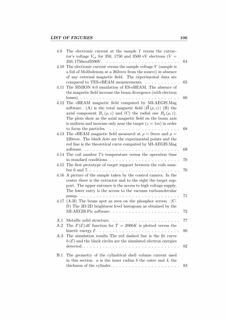
LIST OF FIGURES 100
4.9 The electronic current at the sample I versus the extrac-tor’s voltage Vex for 350, 1750 and 3500 eV electrons (V =350, 1750and3500V . . . . . . . . . . . . . . . . . . . . . . . . 64
4.10 The electronic current versus the sample voltage V (sample isa foil of Molibdenum at a 262mm from the source) in absenceof any external magnetic field. The experimental data arecompared to TES-eBEAM measurements. . . . . . . . . . . . 65
4.11 The SIMION 8.0 simulation of ES-eBEAM. The absence ofthe magnetic field increase the beam divergence (with electronlosses). . . . . . . . . . . . . . . . . . . . . . . . . . . . . . . . 66
4.12 The eBEAM magnetic field computed by MI-AEGIS.Magsoftware. (A) is the total magnetic field | ~B (ρ, z) | (B) theaxial component Bz (ρ, z) and (C) the radial one Bρ (ρ, z).The plots show as the axial magnetic field on the beam axisis uniform and increase only near the target (z = 1m) in orderto focus the particles. . . . . . . . . . . . . . . . . . . . . . . 68
4.13 The eBEAM magnetic field measured at ρ = 0mm and ρ =220mm. The black dots are the experimental points and thered line is the theoretical curve computed by MI-AEGIS.Magsoftware . . . . . . . . . . . . . . . . . . . . . . . . . . . . . . 69
4.14 The coil number 7’s temperature versus the operation timein standard conditions. . . . . . . . . . . . . . . . . . . . . . . 70
4.15 The first prototype of target support between the coils num-ber 6 and 7. . . . . . . . . . . . . . . . . . . . . . . . . . . . . 70
4.16 A picture of the sample taken by the control camera. In thecenter there is the extractor and to the right the target sup-port. The upper entrance is the access to high voltage supply.The lower entry is the access to the vacuum turbomolecularpump. . . . . . . . . . . . . . . . . . . . . . . . . . . . . . . . 71
4.17 (A-B) The beam spot as seen on the phosphor screen. (C-D) The 3D-2D brightness level histogram as obtained by theMI-AEGIS.Pic software. . . . . . . . . . . . . . . . . . . . . . 72
A.1 Metallic solid structure. . . . . . . . . . . . . . . . . . . . . . 77A.2 The P (E) dE function for T = 2000K is plotted versus the
kinetic energy E . . . . . . . . . . . . . . . . . . . . . . . . . . 80A.3 The simulation results The red dashed line is the fit curve
h (E) and the black circles are the simulated electron energiesdetected. . . . . . . . . . . . . . . . . . . . . . . . . . . . . . . 82
B.1 The geometry of the cylindrical shell volume current usedin this section. a is the inner radius b the outer and L thethickness of the cylinder. . . . . . . . . . . . . . . . . . . . . . 83

LIST OF FIGURES 101
B.2 Comparison between MI-AEGIS.Mag results and the E. Den-nison’s equation. The simulated solenoid has a = 14cm,b = 19cm, L = 5cm, I = 7A, 180 wires and centred in(ρ = 0, z = 1m). . . . . . . . . . . . . . . . . . . . . . . . . . . 87
B.3 The laboratory frame used for the axial magnetic field mea-surements. . . . . . . . . . . . . . . . . . . . . . . . . . . . . . 88
B.4 The wire’s number statistical distribution obtained by fittingthe experimental dataset with the MI-AEGIS.Mag theoreticalcalculations. . . . . . . . . . . . . . . . . . . . . . . . . . . . . 89
B.5 The axial magnetic field Bz (ρ, z) vs the hight h at depthd = 3.5cm. The black dots are the experimental data and thered line represents the theoretical model. . . . . . . . . . . . . 89
B.6 The axial magnetic field Bz (ρ, z) vs the depth d at highth = 14.2cm. The black dots are the experimental data andthe red line represents the theoretical model. . . . . . . . . . 90
B.7 A picture of the low-cost homemade gaussmeter. . . . . . . . 91B.8 The electronic sheme of the gaussmeter. . . . . . . . . . . . . 92B.9 The axial magnetic field intensity measured in the center of
one coil (i.e. the output current generated by the Hall probe)vs its circulating current. . . . . . . . . . . . . . . . . . . . . 92
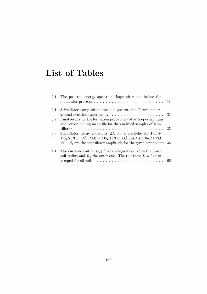
List of Tables
2.1 The positron energy spectrum shape after and before themoderator process. . . . . . . . . . . . . . . . . . . . . . . . . 11
3.1 Scintillator composition used in present and future under-ground neutrino experiment. . . . . . . . . . . . . . . . . . . 31
3.2 Final results for the formation probability of ortho-positroniumand corresponding mean life for the analysed samples of scin-tillators. . . . . . . . . . . . . . . . . . . . . . . . . . . . . . . 35
3.3 Scintillator decay constants ∆ti for β particles for PC +1.5g/l PPO [59], PXE + 1.0g/l PPO [60], LAB + 1.0g/l PPO[60]. Ni are the scintillator amplitude for the given component. 35
4.1 The current-position (zc) final configuration. Ri is the innercoil radius and Ro the outer one. The thickness L = 54mmis equal for all coils. . . . . . . . . . . . . . . . . . . . . . . . 66
102