1

The 4th International Symposium - Supercritical CO2 Power Cycles September 9-10, 2014, Pittsburgh, Pennsylvania

STUDY OF A SUPERCRITICAL CO2 TURBINE WITH TIT OF 1350 K FOR BRAYTON CYCLE WITH 100 MW CLASS OUTPUT: AERODYNAMIC ANALYSIS OF STAGE 1 VANE

Joshua Schmitt University of Central Florida

Orlando, FL, USA joshua.schmitt@gmail.com

David Amos University of Central Florida

Orlando, FL, USA david.amos@ucf.edu

Chad Custer CD-adapco

Northville, MI, USA chad.custer@cd-adapco.com

Rachel Willis University of Central Florida

Orlando, FL, USA nep2112@knights.ucf.edu

Jayanta Kapat

University of Central Florida Orlando, FL, USA

jayanta.kapat@ucf.edu

Joshua Schmitt

Joshua is a Master of Science degree candidate in Mechanical Engineering at the University of Central Florida. He is also currently working for Siemens Energy in their materials and testing division. He received his B.S. in Mechanical Engineering from the University of Florida. He was inducted into the Pi Tau Sigma engineering honor society

Rachel Willis

Rachel is an undergraduate student in her senior year studying mechanical engineering at the University of Central Florida. She has been an undergraduate research assistant for Dr.Kapat at the CATER laboratory. She is the Vice President of the ASME chapter at the University of Central

David Amos

David is the Senior Technical Advisor for CATER Lab at University of Central Florida He graduated with a B.S. and M.S. in Mechanical Engineering from Columbia University. He worked for Westinghouse and Siemens Energy and holds 12 patents in the area of power generation technology. He has been awarded the Westinghouse Lamme Scholarship Award, the George Westinghouse Signature Program Bronze Award, and the Siemens Business Continuity Recognition Award.

2

Jayanta Kapat

Professor Jay Kapat is currently the director of the Center for Advanced Turbines and Energy Research (CATER). Dr. Kapat joined UCF as an assistant professor in August 1997 and he has been a full professor at UCF since August 2005. He has more than 16 years research experience in the areas advanced turbines and energy systems: aerodynamics and heat transfer for gas turbines and other turbomachineries; and miniature Engineering Systems, micro-scale fluidics, heat transfer and related sensors with application to MEMS.

Chad Custer

Chad Custer received his undergraduate degrees in Physics and Mathematics from Gustavus Adolphus College. His graduate research at Duke University focused on harmonic balance numerical methods development. He implemented these methods into the NASA code OVERFLOW and created a harmonic balance version of the solver. This research was funded by a NASA research fellowship, which allowed him to conduct portions of my graduate work at the NASA Langley Research Center. After completing his PhD in 2009, he began with CD-adapco as a Pre-sales engineer. In

2012 he moved to the business development group as the turbomachinery technical specialist.

ABSTRACT

This study seeks to design the aerodynamic features of a first stage vane for a 100 MW class supercritical CO2 Brayton cycle turbomachine. For a turbine inlet temperature of 1350 K, the basic recuperated configuration is found to provide the highest combination of simplicity and cycle efficiency, and the corresponding cycle parameters are then used to design the turbine stages. A 6-stage turbine is selected and the first stage is designed following a one-dimensional mean line approach. Initial mean line turbomachine parameters (work coefficient and flow coefficient) are selected to provide high thermodynamic efficiency and simple radial equilibrium equation principles. Turning loss correlations are utilized to define and optimize hub and casing velocity triangle parameters. Typical turbomachinery characteristic parameters are used to compare the carbon dioxide turbine with typical air combustion turbines. Detailed aerodynamic analysis is performed on a complete three-dimensional model of the vane flow field using a commercial computational fluid dynamics code, STAR-CCM+. Actual properties of the working fluid are input to the model from the REFPROP database provided by the US National Institute of Standards and Technology (NIST). The detailed flow field is computed, from which aerodynamic loss coefficients are calculated. The computer model confirms that the design is successful in turning supercritical carbon dioxide at the prescribed angle and pressure. However, results of the real fluid simulation show that aerodynamic losses caused the stage efficiency to be about 4% below the design target.

INTRODUCTION

The most common working fluids used in Brayton-cycle turbomachinery are air and steam. Other working fluids that are being studied in Brayton cycle applications include supercritical carbon dioxide (Dostal et al, 2004), fluorocarbons, and helium (No et al, 2007). This study focuses on SCO2 as the working fluid.

Supercritical carbon dioxide as the working fluid in a Brayton cycle engine has economic potential in the power generation industry (Dostal et al, 2004). This closed cycle system circulates dense carbon dioxide, through a compressor and turbine to extract work via a shaft. Energy is added to and removed from the working fluid through heat exchangers. This allows the heat energy to come from a variety or combination of sources including concentrated solar power. This paper is built from our previous studies in optimizing a SCO2 Brayton cycle for use with solar power (Schmitt et al, 2013).

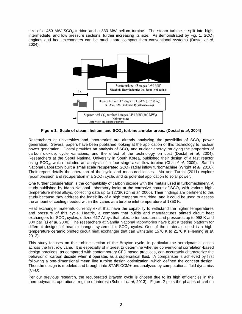
One key benefit of using carbon dioxide can be seen in Fig. 1, where the contrasting turbine scales are shown for various working fluids. In the figure, the size of a 250 MW steam turbine is compared to the

3

size of a 450 MW SCO2 turbine and a 333 MW helium turbine. The steam turbine is split into high, intermediate, and low pressure sections, further increasing its size. As demonstrated by Fig. 1, SCO2 engines and heat exchangers can be much more compact then conventional systems (Dostal et al, 2004).

Figure 1. Scale of steam, helium, and SCO2 turbine annular areas. (Dostal et al, 2004)

Researchers at universities and laboratories are already analyzing the possibility of SCO2 power generation. Several papers have been published looking at the application of this technology to nuclear power generation. Dostal provides an analysis of SCO2 and nuclear energy, studying the properties of carbon dioxide, cycle variations, and the effect of the technology on cost (Dostal et al, 2004). Researchers at the Seoul National University in South Korea, published their design of a fast reactor using SCO2, which includes an analysis of a four-stage axial flow turbine (Cha et al, 2009). Sandia National Laboratory built a small scale recuperated SCO2 radial inflow turbomachine (Wright et al, 2010). Their report details the operation of the cycle and measured losses. Ma and Turchi (2011) explore recompression and recuperation in a SCO2 cycle, and its potential application to solar power.

One further consideration is the compatibility of carbon dioxide with the metals used in turbomachinery. A study published by Idaho National Laboratory looks at the corrosive nature of SCO2 with various high-temperature metal alloys, collecting data up to 1273K (Oh et al, 2006). Their findings are pertinent to this study because they address the feasibility of a high temperature turbine, and it could be used to assess the amount of cooling needed within the vanes at a turbine inlet temperature of 1350 K.

Heat exchanger materials currently exist that have the capability to withstand the higher temperatures and pressure of this cycle. Heatric, a company that builds and manufactures printed circuit heat exchangers for SCO2 cycles, utilizes 617 Alloys that tolerate temperatures and pressures up to 998 K and 300 bar (Li et al, 2008). The researchers at Sandia National laboratories have built a testing platform for different designs of heat exchanger systems for SCO2 cycles. One of the materials used is a high-temperature ceramic printed circuit heat exchanger that can withstand 1570 K to 2170 K (Fleming et al, 2013).

This study focuses on the turbine section of the Brayton cycle, in particular the aerodynamic losses across the first row vane. It is especially of interest to determine whether conventional correlation-based design practices, as compared with contemporary CFD based practices, can accurately characterize the behavior of carbon dioxide when it operates as a supercritical fluid. A comparison is achieved by first following a one-dimensional mean line turbine design optimization, which defined the concept design. Then the design is modeled and brought into STAR-CCM+ and analyzed by computational fluid dynamics (CFD).

Per our previous research, the recuperated Brayton cycle is chosen due to its high efficiencies in the thermodynamic operational regime of interest (Schmitt et al, 2013). Figure 2 plots the phases of carbon

4

dioxide in terms of pressure and temperature. Shaded regions show where carbon dioxide is a solid, liquid, or gas. After a certain temperature and pressure is reached, beyond the critical point, the carbon dioxide becomes a supercritical fluid. This can be seen in Fig. 2 as a white region bounded by dotted lines.

Also in Fig. 2 is a graphical representation of the recuperated Brayton cycle. The blue lines represent the working fluid as it travels through the cycle from one state point to another with arrows indicating the direction the fluid circulates. The numbers in Fig. 2 represent the key state points of the working fluid as it moves from compressor to turbine and through heat exchangers. These state points correspond to the values tabulated in Table 1.

Work is extracted by a turbine between state points 3 and 4. The work required to compress the fluid is added between points 1 and 2. The recuperator is a heat exchanger that extracts heat from the hot fluid exiting the turbine at point 4 and transfers it to the colder fluid leaving the compressor at point 2.

This flow of heat from the low pressure to the high pressure part of the cycle is represented in Fig. 2 by arrows and a shaded region in the center of the cycle. Point 5 on the diagram represents the state point of the heated, high-pressure fluid leaving the recuperator. Similarly, point 6 is the temperature and pressure reached by the low pressure fluid after the recuperator cools it. This provides a massive rise in efficiency because it greatly reduces the heat added from the energy source, shown in Fig.2 between points 5 and 3 and is represented by a large arrow. From point 6 to 1 heat is rejected to the environment by a heat exchanger, which is also indicated by an arrow in Fig. 2.

Figure 2. P-T diagram of the recuperated SCO2 Brayton cycle.

The turbine in this study is designed to be a 100MW class turbine with a turbine inlet temperature of 1350 K. These can be considered the static parameters, and in all the iterations of the engine design, these did not change.

To achieve this, the mass flow rate is varied, along with the compressor pressure ratio. The critical point of carbon dioxide is at 7.39 MPa and 304.25 K. Because SCO2 operates under high pressures, the pressure ratio could not reasonably be set above 4.0 across the compressor. This was chosen so the highest pressures reached were within the operational realm of state of the art ultra-supercritical steam turbine technology (Schmitt et al, 2013). Under this condition the mass flow rate is calculated to be 487 kg/s.

The efficiencies and losses at each stage of the cycle are postulated, and must be confirmed later in the design. Our initial estimates set concept design requirements with a 90% efficiency objective in the turbine, 85% in the compressor, and a 4.0% loss in pressure through each heat exchanger. The

5

effectiveness of the recuperator is selected to be 90%. The properties of carbon dioxide are sourced directly from the NIST REFPROP database (Lemmon et al, 2010). Using REFPROP, the cycle state points are found and listed in Table 1. The key state point to this study is state point 3, which represents the turbine inlet fluid conditions.

Table 1. Brayton cycle state points

State Point

Temp.

(K)

Pressure

(MPa)

Density

(kg/m3)

Enthalpy

(kJ/kg)

Entropy

(kJ/kg-K)

1 305.37 7.688 579.96 310.92 1.3617

2 353.41 30.751 751.83 350.16 1.3787

3 1350 28.431 104.25 1713.6 3.3059

4 1145.1 8.315 37.707 1445.6 3.3322

5 1065.9 29.567 136.91 1340.0 2.9874

6 331.9 7.996 194.20 455.8 1.8225

If the assumed efficiencies are met the total cycle efficiency was calculated to be approximately 60%, a very competitive value for power companies and turbine manufacturers. With these cycle points as a starting point, we begin the design of the 90% efficient SCO2 turbine.

DESIGN METHODOLOGY

The turbine input and output thermodynamic state points are known, as shown in Table 1. From these inputs we begin to optimize the design of the turbine section. We start from a one-dimensional mean line approach, where the mean-line radius remains constant and the annular area increases uniformly from the first to the last stage. This method and its ability to estimate turbine efficiency is detailed by Dixon and Horlock (1975, 1966). With this design, the height of the blade is calculated using the density and mass flow, as shown in Eq. 1.

(1)

With this and the density at State Point 1 from Table 1, the height of the blade can be determined by varying the mean radius and the flow velocity. The mean radius was selected to correspond to an initial mean-line wheel velocity that provided a reasonable velocity triangle when balanced with the axial flow velocity. The radius was then tweaked when the inlet vane height was found to be unfeasible. The flow entering the first row of the turbine was designed to be axial and equal to . In addition, this axial component of velocity is chosen to remain constant throughout the turbine.

(2)

The wheel speed, or tangential velocity, of the turbine, as shown in Eq. 2, also plays a role in the design of the turbine. In this case, the angular velocity, , is set to correspond with a synchronous 3600 RPM for conventional 60 Hz operation. The wheel speed determines the flow coefficient and loading coefficient,

6

aerodynamic parameters used for the design of the blades and vanes. The flow coefficient, representing the ratio of the axial flow to the wheel speed at the mean line, is shown in Eq. 3. The work coefficient in Eq. 4 depends on the enthalpy change across the stage and is normalized to the wheel speed.

These two coefficients define the basic per-row design of blades and vanes in the one-dimensional mean line approach. We initiate the design of the first row of blades and vanes using these parameters. The design requires us to assume initial values and insert them into the above equations. The wheel speed parameter is varied, also changing the mean line radius as a result.

(3)

(4)

We adjust the work produced by each stage by changing the number of stages in the turbine and the proportion of enthalpy change carried by each stage. The flow coefficient, and hence the axial velocity, is chosen to produce the maximum efficiency, using the conventional Smith Chart in Fig. 3. All of these parameters are adjusted and iterated until the turbine design goals are achieved.

Figure 3. Smith chart relating the design coefficients to total-to-static efficiency (Horlock, 1966).

The goal of our design is to maximize the efficiency of the first stage. At the very least, it must meet the 90% efficiency stipulated in our concept design requirements. Using Fig. 3, we vary the values of the coefficients so the design was at or above the 90% efficiency line. In optimizing these parameters, some interesting concerns arose. The density of the fluid at the inlet, being relatively high, results in comparatively short blade heights. Small vanes and blades can allow secondary flows to dominate the aerodynamics and create an inefficient engine (Horlock 1966). Additionally, at smaller scales more flow can be lost over the tip of the blade, again lowering efficiency. Manufacturing tight tolerances could be difficult and more costly at such small scales. For all of these reasons we choose to set a minimum

7

height of 2 cm when optimizing the design. This suggests that future studies may wish to consider even larger output sizes than the 100MW class to realize larger blading sizes.

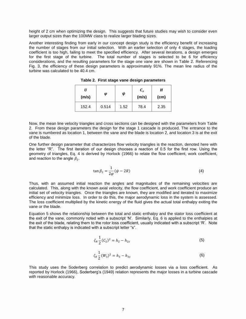
Another interesting finding from early in our concept design study is the efficiency benefit of increasing the number of stages from our initial selection. With an earlier selection of only 4 stages, the loading coefficient is too high, failing to meet the specified efficiency. After several iterations, a design emerges for the first stage of the turbine. The total number of stages is selected to be 6 for efficiency considerations, and the resulting parameters for the stage one vane are shown in Table 2. Referencing Fig. 3, the efficiency of these design parameters is approximately 91%. The mean line radius of the turbine was calculated to be 40.4 cm.

Table 2. First stage vane design parameters

(m/s)

(m/s)

(cm)

152.4 0.514 1.52 78.4 2.35

Now, the mean line velocity triangles and cross sections can be designed with the parameters from Table 2. From these design parameters the design for the stage 1 cascade is produced. The entrance to the vane is numbered as location 1, between the vane and the blade is location 2, and location 3 is at the exit of the blade.

One further design parameter that characterizes flow velocity triangles is the reaction, denoted here with the letter “R”. The first iteration of our design chooses a reaction of 0.5 for the first row. Using the geometry of triangles, Eq. 4 is derived by Horlock (1966) to relate the flow coefficient, work coefficient, and reaction to the angle .

( ) (4)

Thus, with an assumed initial reaction the angles and magnitudes of the remaining velocities are calculated. This, along with the known axial velocity, the flow coefficient, and work coefficient produce an initial set of velocity triangles. Once the triangles are known, they are modified and iterated to maximize efficiency and minimize loss. In order to do this, the major aerodynamic loss in the system is assessed. The loss coefficient multiplied by the kinetic energy of the fluid gives the actual total enthalpy exiting the vane or the blade.

Equation 5 shows the relationship between the total and static enthalpy and the stator loss coefficient at the exit of the vane, commonly noted with a subscript ‘N'. Similarly, Eq. 6 is applied to the enthalpies at the exit of the blade, relating them to the rotor loss coefficient, usually indicated with a subscript ‘R’. Note that the static enthalpy is indicated with a subscript letter “s”.

( )

(5)

( )

(6)

This study uses the Soderberg correlation to predict aerodynamic losses via a loss coefficient. As reported by Horlock (1966), Soderberg’s (1949) relation represents the major losses in a turbine cascade with reasonable accuracy.

8

Soderberg’s relation, shown in Eq. 7, uses the overall angular deflection in degrees, , to estimate the

loss coefficient, . The total angular deflection across the vane is the sum of and ; the angular deflection across a blade is the sum of and . The loss coefficient is utilized to estimate the total-to-total and total-to-static efficiencies of the row.

[ (

)

] (7)

The total-to-total efficiency is defined as the actual difference in total enthalpy from 1 to 3 across the row divided by the ideal, no-loss difference in total enthalpy. The total-to-static efficiency is similar, but the difference in total enthalpy is now divided by the difference in total enthalpy at 1 and the ideal, static enthalpy at 3. Combining these definitions and Eqs. 5 and 6, expressions relating the efficiency to velocity magnitudes are derived. Knowing the geometry of a velocity triangle, the equations are written in terms of the flow coefficient and the relative and absolute angles. The final form of these equations is seen in Eqs. 8 and 9.

[

⁄

⁄

]

(8)

[

⁄

⁄

]

(9)

Equations 8 and 9 allow the use of Soderberg’s relation across the stationary and the rotating sections to calculate the efficiency of the design. In this study, we begin with our initial design and find the loss coefficients. Then, we check our calculated efficiency versus the targeted efficiency of 90%. The efficiency of the initial design was below target, so the process is iterated until 90% total-to-total efficiency was achieved. The flow angle at the vane exit, , is varied by a few degrees from the 0.5 reaction design. The 90% efficiency criterion is met when the angle is increased, and the stage reaction decreased. The solution here is found after much iteration. The 90% criterion can be reached through many different designs, depending on which parameters are restricted and prioritized.

Figure 4. First row mean-line velocity triangles and corresponding cross sections.

9

The resulting mean line triangles for this study are shown in Fig. 4, along with blade and vane cross sections. In Fig. 4, the top right indicates the cylindrical coordinate system used when plotting the velocity triangles. Also, the flow inlet angle, , is 0°, corresponding to the design choice of purely axial inlet flow. A list of the angles, reaction, loss coefficients and efficiencies is found in Table 3.

Using Eq. 1 and knowing the mean-line radius, the mass flow rate, and density exiting the first row of the turbine, the height is calculated to be 2.79 cm. The density after the blade is referenced using the REFPROP software after subtracting out the predicted loss in enthalpy and pressure and using these new values as state points. This allowed for a design choice where the hub and casing radii decrease and increase at the same rate. As a result, the casing and the hub have the same outward slope. Knowing this, the hub and casing radii of the first row blade are calculated.

Substituting the radius at the hub and the casing into Eq. 2, a wheel speed at these locations was found. The specification of a free vortex flow inside the turbine, to satisfy radial equilibrium requirements, is made to calculate the flow velocities at the hub and the casing. In this case, a free vortex is defined as irrotational flow that moves through the turbine cascade. Under a free vortex, the product of the radius and the absolute tangential velocity remains constant at any location. This allows for the relationship shown in Eq. 10.

The subscript “θ”, indicates the velocity component in the direction tangential to the radius. Thus, new velocity triangles can be found at the hub and the casing utilizing Eq. 10 and the respective wheel speeds. The flow hub and casing angles, reaction, loss coefficients, and efficiencies are in Table 3. All angles in Table 3 are in degrees, the remaining parameters are dimensionless.

Table 3. First row aerodynamic design results

Cross section Mean Hub Casing

φ 0.514 0.529 0.500

(º) 70.7 71.2 70.2

(º) 5.7 5.9 5.6

(º) 42.3 46.5 37.7

(º) 63.9 63.3 64.5

(º) 70.7 71.2 70.2

(º) 106.3 109.8 102.3

R 0.292 0.249 0.331

0.070 0.070 0.070

0.108 0.112 0.103

(%) 0.903 0.900 0.905

(%) 0.835 0.832 0.837

(10)

10

This fully defines the cross sections of the first row vanes and blades, and a three-dimensional model can be laid out. The dimensions governing the design of the first row vanes’ shape are height, chord, pitch, and axial width. The height is already determined earlier to vary from 2.35 cm to 2.79 cm, making the average height 2.57 cm. In order to select the vane chord, we look at a study of losses reported by Ainley and Mathieson (1967).

Figure 5 shows how aspect ratio affects the losses across an airfoil. Note that the heights and chords in Fig. 5 are listed in inches. An aspect ratio of 1.0 is chosen as a balance between losses and an achievable chord length. Because this turbine operates on a small scale, increasing the aspect ratio would reduce losses to a minor degree, but the chord would diminish. If the selected chord is too short the pitch is affected and it might be impractical to provide the proper turning angles needed in the vane.

Figure 5. Aspect ratio and loss correlation (Ainley and Mathieson, 1967).

The loss coefficient at an aspect ratio of 1.0 is between 0.07 and 0.08, according to Fig. 5. This loss is deemed acceptably close to the Soderberg loss and thus the vane should not experience much additional loss due to the aerodynamic design. The chord is designed to be constant from the hub to the casing of the vane, and, based on the average height and aspect ratio, the chord has a value of 2.57 cm.

The axial width of the vane was determined using Eq. 11. In this equation, the average of the inlet and outlet flow angles is taken to be the stagger angle of the vane, which represents the angle of the chord from the axial direction. Then the cosine and the chord length are used to find the width. The stagger angle is 35.4°, and the width was 2.10 cm.

(11)

The final step in designing the first row vanes is determining the pitch. The Zweifel parameter is used in minimizing the pressure loss coefficient in a cascade. Zweifel’s findings (1945) indicated that a value equal to nominally 0.8 provides the minimum amount of loss across this design and thus the optimum pitch at the mean line pitch. Zweifel formulates the relationship between Zweifel’s parameter, pitch, width and the inlet and exit flow angles across a vane, which is shown in Eq. 12, as reported by Dixon (1975).

⁄

( ) ( )

( ) (12)

The ideal pitch at the mean line is solved for in Eq. 12, producing a value of 2.69 cm. When sketching the airfoil shape and spacing, the distance between the vanes appears problematic. The throat of the vane

11

passage, the localized flow area between the trailing edge of an airfoil and the subsequent airfoil’s suction side, is judged to be too wide. The tangent angle to the throat area does not meet our specified angle, indicating that the flow may not follow the design parameters. To remedy this, the pitch is shortened and iterated until the throat tangent angle matches the vane exit angle. The resulting pitch is 1.84 cm. This value corresponds to 138 airfoils in the first row vanes. Under this design, the new Zweifel parameter is 0.55, which is deemed an acceptable deviation.

The three dimensional shape of the airfoil is found by repeating this process at the hub and the casing. The values of the angles are taken from Table 3 and an airfoil cross section is produced. After sketching the profiles at the hub, mean and casing in SolidWorks, we find the centroid of each shape. The profiles are then lined up at the appropriate height but under the constraint of the center of mass of each cross section being kept along the same vertical axis. The three dimensional vane can then be generated from a sweep of these cross sections.

REAL GAS CFD MODELING

The next step of this study is the CFD aerodynamic analysis of the first row vane of our SCO2 turbine design.

(a) (b)

Figure 6. Simple solid model of (a) single first row vane and (b) the stationary section ring assembly.

An isometric view of the single vane design can be seen in Fig. 6a. Notice that the vane segment includes convection cooling holes that are internal to the vane and placed along the camber line of the airfoil. These are added because of the high fluid temperatures entering the vane. It is unlikely that conventional nickel-based superalloy vanes could survive these temperatures without some form of internal cooling. Figure 6b shows how all 138 vane segments come together to form the first row stationary ring.

Similarly, Fig. 7 is the solid modelling of the rotating section of the first stage. Figure 7a is an isometric view of the rotating airfoil, and Fig. 7b demonstrates how these airfoils are installed in a grooved disk. A sensitivity check was done on Eq. 8. It is found that under our design the change in total-to-total efficiency is more sensitive to the Soderberg loss coefficient in the vane than the Soderberg loss coefficient in the rotor. The effect of difference in the vane loss coefficient is about 130% greater than the

12

effect of changing the rotor loss coefficient. Thus, the vane is more important to achieving the 90% total-to-total efficiency. For this reason, and to help focus the scope of the paper, only the vane is simulated in CFD.

(a) (b)

Figure 7. Simple solid model of (a) single first row blade and (b) the rotating disk and blade assembly

The single vane segment model is imported into STAR-CCM+ for meshing. The geometry of the model is subtracted from a larger geometry surrounding the model so that the three-dimensional body represents the fluid around the vane, not the vane itself. The three-dimensional model is then converted into an unstructured mesh with approximately 2.7M polyhedral cells. Fifteen body fitted prism layers are implemented to resolve the boundary layers on the vane. For these boundary layers, the first cell thickness is 2.5e-6 cm, and the total prism layer thickness is 0.02 cm. The overall mesh with a mid-span slice is presented in Fig. 8a. Figure 8b gives a detailed view of the prism layer and unstructured mesh.

(a) (b)

Figure 8. CFD input grid (a) overall view and (b) mean-line mesh.

In order to capture all of the features of the flow entering and leaving the vane, the grid is extended by approximately 1.5 cm in the axial direction at the inlet and exit. This extension at the exit is an overly large

13

estimation of the gap needed between the vane and blade. This is to ensure that trailing edge turbulence was captured in the computer model. After reviewing the results of the paper, the turbulent wake of the trailing edge of the vane can be studied. In future designs, the gap between vane and blade can be shortened.

(a) (b)

Figure 9. Cp and Viscosity variation of SCO2 (a) up to 1350 K with (b) detailed view near critical point.

Figure 9 charts a parametric study of the behavior of CO2 with increases in temperature and pressure. The data is taken directly from the REFPROP database (Lemmon et al, 2010) and graphed versus temperature. Each line represents a constant pressure line. Figure 8a displays the full range of temperatures and pressures relevant to this study. The constant pressure lines vary from 5 MPa to 28 MPa and the values for each line are labelled in Fig. 9b. Blue lines represent viscosity variation, corresponding to the axis on the right, and green lines plot the constant pressure specific heat as it changes with temperature.

As detailed in Fig. 9b, the particularly interesting region lies in the lower temperatures. This domain is near the critical temperature. Both viscosity and specific heat experience large property variations, depending on pressure. This behavior of carbon dioxide can cause design complications.

Checking values from Table 1, the compressor operates well within this problematic region, but most temperatures in the turbine element, the subject of this paper, operate above 1000 K, well away from regions of complicating large property variations. Now, looking at Fig. 8a, the constant pressure lines converge to a single line for temperatures above 560 K. Thus, for the CFD calculations of the first row vane, specific heat and viscosity are input as solely functions of temperature, not dependent on pressure.

STAR-CCM+ allows us to manually enter the physical properties of the fluid using data generated by REFPROP. The dynamic viscosity and thermal conductivity values are determined from REPROP and placed in a table that was dependent on temperature. Similarly, the specific heat data is curve fit to a fourth-order polynomial that is dependent on temperature. Molecular weight, standard state temperature, and the turbulent Prandtl number are all assumed to be constant. The turbulence model is set to the k-epsilon method. The turbulence is specified to have an intensity of 20% and a length scale of the hydraulic diameter of the passage at the leading edge.

The solution is assumed to be in a steady-state. Constant profile pressure, temperature and flow direction are defined at the inlet boundary condition. The CFD software treats this grid’s boundary condition in the cylindrical direction as periodic, a built-in feature of the code. The inlet boundary condition total temperature and total pressure are taken from Table 1 and specified to be constant across the entire radial profile. The axial flow velocity at the inlet, , is specified to be constant across the entire inlet area. The boundary condition of the “metal” surfaces, where the fluid would touch the vane, hub, or casing, are chosen to have an adiabatic, no-slip boundary condition.

14

The outlet static pressure at the hub is estimated to be 25.474 MPa using the mean-line velocity triangles. This is specified as the constant outlet boundary condition value for STAR-CCM+ to check against as it converges on the specified mass flow rate. Once the CFD software is fully configured, a solution was generated.

RESULTS

The results of our computer model provide insight into the success of our one-dimensional mean-line design of a SCO2 turbine. The software converges on a mass flow rate of 487.0 kg/s, which matches the design parameter, and, since the solution is calculated correctly, the mesh is deemed satisfactory.

Table 4. Mass flow averaged CO2 properties

inlet exit

Total Pressure (MPa) 28.43 28.20

Static Pressure (MPa) 25.69 25.69

Total Temperature (K) 1350.0 1350.0

Static Temperature (K) 1347.9 1332.2

Total Enthalpy (kJ/kg) 1713.6 1713.6

Static Enthalpy (kJ/kg) 1710.5 1689.6

Velocity Magnitude (m/s) 78.4 217.2

Flow Angle (º) 0 71.2

The key flow characteristics output by the CFD calculations are shown in Table 4. The values in Table 4 are all averaged based on mass flow. These average values can provide some initial insight into the behavior of the blade design. The magnitude of the exit velocity from CFD is 10.8% lower than the concept design velocity, which is 243.49 m/s.

Figure 10 demonstrates how the velocity changes in magnitude and direction at the mean-line radius. The results from Table 4 indicate that the flow exited at an angle of 71.2 degrees, a 0.71% increase from the design angle. This is a small deviation, and thus these vanes are considered to be successfully turning the flow to the proper angle. In Fig. 10, the gray zone is overlaid, showing the grid as it is represented in this slice. It is apparent from this view how STAR-CCM+ treated a single airfoil as periodic and was able to provide a solution for all of the vanes. Importantly, there is a stagnation point at the front of the airfoil and the wake at the trailing edge. These areas of low flow lead to the hotter temperature zones seen in Fig. 13.

The direction of the flow in Fig. 10 adequately turns and follows the airfoil exit angle. This indicates the design was acceptable for achieving the desired flow directions. The flow exiting the vane has periodic highs and lows due to the lower velocity wake emanating off the trailing edge of the vane. This may be improved by decreasing the radius of the trailing edge. The effect of this behavior on pressure and temperature can be seen in Figs. 11 and 12.

15

Figure 10. CFD calculated output in flow velocity and at the mean-line.

Figure 11 graphs the pressure and temperature variation in the design traversing from the inner radius to the outer radius at the vane exit along the mid-point between the trailing edges. The red data in Fig. 11 represents the static value and the blue data the total or stagnation values of temperature and pressure. In Fig. 11, notice how the static temperatures and pressure rose from hub to casing. This indicates that the dynamic temperature and pressure were decreasing, and, therefore, the velocity of the flow also decreased.

(a) (b)

Figure 11. with varying radius, (a) pressure and (b) temperature at the mid-point between trailing edges of two vanes

Since the velocity is higher at the hub and lower at the casing, the CFD results behave in the manner of a free vortex. In fact, checking the velocities versus the design calculations, they only deviate from the free vortex condtion by at most 3%. Thus, our early design decision to model based on the principles of free vortex flow is confirmed.

Figure 12 shows the total pressure distribution leaving the vane in an axial slice. Specifically, the slice is taken just after the trailing edge tip of the airfoil. In this slice, the vanes are generally pointing the flow in

16

a downward direction. The behavior of the fluid near the vane hub, casing, and at the trailing edge can be seen here to be creating secondary flows and causing low pressure regions. These secondary flows are likely the primary contributor to loss in the vane. In order to provide a more uniform pressure to the blades, these low pressure regions should be minimized. Two possible ways of achieving this are decreasing the radius at the trailing edge or widening the pitch by selecting fewer airfoils.

Figure 12. Vane exit total pressure in the r-θ plane

Figure 13 displays the temperature distribution across the vane under the adiabatic boundary condition. The pressure side experienced much hotter conditions than the suction side. This behavior is expected because the fluid is impinging on the pressure side, causing a rise in temperature. The suction side does not feel this effect and is much cooler. The coldest zone on the suction side is just before the throat. It is suggested that future changes to the airfoil push the curvature outward to out the surface temperature before the throat. Concentrations of temperature can be important for designing the vanes’ internal cooling system. The temperatures reached on the surface of the vane may be too hot for the materials to withstand.

Figure 13. Temperature variance across a vane in the adiabatic case

17

As stated by Horlock (1966), the aerodynamic loss coefficients are largely the same in a cooled turbine, as long as the cooling flow remains internal. For the temperatures seen in Fig. 13, it is assumed that internal cooling will be sufficient to allow the part to survive. Furthermore, efficiency will only decrease from the adiabatic case because heat is lost. Thus the verification of the Soderberg correlation is the most optimistic in the adiabatic case. In practice it will be necessary to add and optimize cooling in this turbine, but ultimately the detailed cooling design is beyond the scope of the paper. There are many possible cooling solutions that can be considered for this design, and they will be the subject of future research.

The total pressure between the inlet and the exit drops by 230 kPa, which is 0.81% less than the total inlet pressure. The design case estimates a pressure loss of only 125 kPa, a 0.44% reduction in total pressure. Using these pressure losses, the pressure loss coefficient is found. The CFD calculation places the pressure loss coefficient at 0.102, whereas the design loss coefficient was only 0.044.

Next, the enthalpy losses are considered. Equation 5 gives the relationship between the loss coefficient, the flow velocity leaving the blade, and the difference in enthalpy between the real vane and an isentropic vane. The design enthalpy difference is 2.08 kJ/kg. The CFD results indicate a 3.30 kJ/kg difference in enthalpies, which is a higher loss. Applying Eq. 5 to the CFD results, the new loss coefficient is 0.140. The design loss coefficient from Table 3 is 0.070. It is notable that both the pressure loss coefficient and the enthalpy loss coefficient increase by comparable amounts for the real gas model. The higher loss coefficient may indicate lower overall turbine efficiency.

The CFD loss and flow angle values are introduced into Eqs. 8 and 9, while the rotating section is kept the same as the design case. The new total-to-total efficiency of the stage is 85.7% and the new total-to-static efficiency is found to be 79.2%. These represent significant drops in efficiency from the design objective case.

CONCLUSIONS

Overall, the design process for a SCO2 turbine was found to be similar to the design of conventional turbine systems with a few special considerations. The challenges to the design largely stem from the high pressure and density of the supercritical fluid. The high pressures require the turbine to be housed in a thick-walled pressure vessel, increasing internal stresses. High densities make for much smaller flow paths and shorter airfoils. If the turbine is too small, the blades may be too short to control the flow without tip losses and other secondary flows, even in a 100 MW sized turbine. Thus, a SCO2 system may require sizing above 100 MW to be an efficient design. Because the airfoils are sharing large loads, more stages are needed to prevent high per-stage loading, which would cause excessive stresses to the diminutive turbomachinery. Small airfoils would make blade cooling much more difficult to manufacture, potentially limiting the maximum turbine inlet temperature. Thus, the conventional design process can create a SCO2 turbine but with some limitations. Some design innovations may be needed for SCO2 to perform at the level and flexibility of conventional gas turbines.

The overall design of the first row vane is successful. However, the overall efficiency calculated using CFD is found to be lower than expected using Soderberg loss calculations. The design of the first set of vanes is initially generated using a one-dimensional mean-line approach. The aerodynamic parameters are then modeled into STAR-CCM+, a CFD software package.

The computer model demonstrates that the supercritical fluid successfully turned through the vane to produce aerodynamic flow angles similar to the design case. The CFD model also successfully converges on the design flow rate, and although the estimated efficiency in the turbine dropped, it is still high enough to provide enough power for a 100 MW class power cycle.

However, the CFD predicts significantly larger losses in pressure and enthalpy for the adiabatic vane. This suggests that for a SCO2 turbine operating at the scales outlined here, the Soderberg loss coefficient is not sufficient alone to estimate the entirety of the primary loss. Further study is recommended to determine which additional losses should be factored into the design of an SCO2 turbine.

18

NOMENCLATURE

= Axial Flow Absolute Velocity, m/s

= Annular Height, cm = Mean-line Radius, cm

= Mean-line Wheel Speed, m/s

= Angular Velocity, rad/s = Flow Coefficient

= Work Coefficient SCO2 = Supercritical Carbon Dioxide CFD = Computational Fluid Dynamics = Mass Flow Rate, kg/s

= Density, kg/m3

= Enthalpy, kJ/kg = Total-to-Static Efficiency, %

= Total-to-Total Efficiency, %

= Row Reaction

= Flow Absolute Velocity, m/s = Flow Relative Velocity, m/s

= Flow Absolute Angle, degree (°)

= Flow Relative Angle, degree (°) = Loss Coefficient

= Airfoil Axial Width, cm

= Airfoil chord, cm = Airfoil pitch, cm

= Zweifel Parameter

19

REFERENCES

Ainley, D. G., and Mathieson, G. C. R., 1967, “A Method of Performance Esitmation for Axial Flow Turbines”, London.

Cha, J., Lee, T., Eoh, J., Seong, S., Kim, S., Kim, D., Kim, M., Kim, T., Suh, K., 2009, “Development of a Supercritical CO2Brayton Energy Conversion System Coupled with a Sodium Cooled Fast Reactor,” Nuclear Engineering and Technology, Vol. 41, pp 1025-1044.

Dixon, S.L., 1975, “Fluid Mechanics, Thermodynamics of Turbomachinery”, University of Liverpool, Pergamon Press.

Dostal, V., Driscoll, M., Hejzlar, P., 2004, “A Supercritical Carbon Dioxide Cycle for Next Generation Nuclear Reactors”, MIT, Boston, MA.

Fleming, D., Pasch, J., Conboy, T., Carlson, M., 2013, “Testing Platform and Commercialization Plan For Heat Exchanging Systems For SCO2 Power Cycles”, ASME Turbo Expo, pp 1-4.

Horlock, J.H, University of Cambridge, 1966, “Axial Flow Turbines”, Butterworth and Co.

Lemmon, E.W., Huber, M.L., McLinden, M.O., 2010, NIST Standard Reference Database 23: Reference Fluid Thermodynamic and Transport Properties-REFPROP, Version 9.0, National Institute of Standards and Technology, Standard Reference Data Program, Gaithersburg.

Li, X., Kininmont, D., Le Pierres, R., and Dewson, J., 2008 “Alloy 617 for the High Temperature Diffusion-Bonded Compact Heat Exchangers”, Proc. ICAPP ’08, Anaheim, CA.

Ma, Z. and Turchi, C., 2011, “Advanced Supercritical Carbon Dioxide Power Cycle Configurations for Use in Concentrating Solar Power Systems”, Proc. SCO2 Supercritical CO2 Power Cycle Symposium, Boulder, CO, May 24-25

No, H.C., Kim, J.H., Kim H.M., 2007, “A Review of Helium Gas Turbine Technology for High Temperature Gas Cooled Reactors,” Nuclear Energy and Technology, 23(1), pp 21-30.

Oh, C., Lillo, T., Windes, W., Totemeier, T., Ward, B., Moore, R., Barner, R., 2006, “Development of a Supercritical Carbon Dioxide Brayton Cycle: Improving VHTR Efficiency and Testing Material Compatibility”, Idaho National Laboratory, Idaho Falls, Idaho.

Schmitt, J., Willis, R., Amos, D., and Kapat J., 2013, "Feasibility and Application of Supercritical Carbon Dioxide Brayton Cycle to Solar Thermal Power Generation," ASME 2013 Power Conference, Boston, MA.

Soderberg, C. R., 1949, Unpublished note. Gas Turbine Laboratory, Massachusetts Institute of Technology.

Wright, S. A. et al., 2010, “Operation and Analysis of a Supercritical CO2 Brayton Cycle”, Sandia Report No. SAND2010-0171, Sandia National Laboratory, Albuquerque, New Mexico.

Zweifel, O., 1945, “Optimum Blade Pitch for Turbo-Machines with Special Reference to Blades of Great Curvature”; Brown Boveri Review, Vol 32.

ACKNOWLEDGEMENTS

The work is supported solely by the University of Central Florida and performed at Siemens Energy Center – a research laboratory at the University of Central Florida established by Siemens Energy. We would also like to thank CD-adapco for their contributions to this study.

Also a special thanks to Noël Simonovici from the Grenoble Institute of Technology as well as Tiphaine Houssin, Alexandre Ory, and Hélène Trubert from the University of Nantes, for all of their hard work and contributions to help make this paper possible.