STUDY INTO THE POTENTIAL AND FEASIBILITY OF A STANDALONE SOLAR-

WIND HYBRID ELECTRIC ENERGY SUPPLY SYSTEM

For Application in Ethiopia

Doctoral Thesis

By

Getachew Bekele

Department of Energy Technology School of Industrial Engineering and Management

Royal Institute of Technology, KTH Stockholm, December 2009

ii

Study into the Potential and Feasibility of a Standalone Solar-Wind Hybrid Electric Energy Supply System for Application in Ethiopia

Getachew Bekele

TRITA REFR Report No 09/64 ISSN 1102-0245 ISRN KTH/REFR/09/64-SE ISBN 978-91-7415-329-3

Doctoral Thesis by Getachew Bekele

Division of Applied Thermodynamics and Refrigeration

Department of Energy Technology

School of Industrial Engineering and Management

Royal Institute of Technology, KTH

Printed by Universitetsservice US AB Stockholm, 2009

© Getachew Bekele 2009

iii

Abstract

The tendency to use renewable energy resources has grown continuously over the past few decades, be it due to fear over warnings of global warming or because of the depletion and short life of fossil fuels or even as a result of the interest which has developed among researchers doing scientific research into it. This work can be considered as joining any of these groups with an objective of giving electric light to the poor population living in one of the poorest nations in the world.

The aim of the work is to investigate supplying electric energy from solar-wind hybrid resources to remotely located communities detached from the main grid line in Ethiopia. The communities in mind are one of two types; the first is the majority of the poor population residing in the countryside; and the other is people relocated by the Government from the over used and dry regions to relatively productive and fertile ones in line with the long-term poverty reduction plan.

The work was begun by investigating wind energy and solar energy potentials at four geographically different locations in Ethiopia by compiling data from different sources and analyzing it using a software tool. The locations are Addis Ababa (09:02N, 038:42E), Mekele (13:33N, 39:30E), Nazret (08:32N, 039:22E), and Debrezeit (8:44N, 39:02E).

The results related to wind energy potential are given in terms of the monthly Average wind speed, the wind speed probability density function (PDF), the wind speed cumulative density function (CDF), the wind speed duration curve (DC), and power density plots for all four selected sites. According to the results obtained through the analysis, the wind energy potential, even if it is not exceptional, is irrefutably high enough to be exploited for generating electric energy.

The solar energy potential, based on sunshine duration data collected over a period of 7 - 11 years and radiation data obtained from different sources, has been calculated using regression coefficients specific to the sites in question. Based on the sunshine duration data, the monthly average daily sunshine amount for each of the places has also been computed and given in a form of plot. Through additional work on the

iv

results of the calculations, the solar energy potential has been given in the form of solar radiation plots for each of the selected sites. As expected, the results indicated an abundance of solar energy potential.

It is based on the promising findings of these two energy resource potentials, wind and solar, that the feasibility study for a standalone solar-wind hybrid energy supply system has proceeded, targeting the community mentioned earlier. The hybrid system consisted of Wind turbine, Photovoltaic panel, diesel generator and a bank of batteries, with a power conditioning converter included in the system.

The hybrid standalone supply system is intended to provide electricity to a model community of 200 families with five to six family members in each. The community is equipped with a primary load, a deferrable load, a community school and a health post. An electric load which includes lighting, water pumping, a radio receiver, and some clinical equipment has been suggested. Hybrid Optimization Model for Electric Renewables, HOMER, software has been used for the analysis. The average wind speed and average solar radiation calculated from the data for all of the selected sites has been used to input into the software.

The hybrid system design is approached in three different ways. The first approach is to include within the hybrid system those components which are locally available, without giving special attention to their efficiencies and proceed with the design work. The second approach is to thoroughly search the market for the best and most efficient technological products and to select the best components for the analysis. A third approach considered in an attempt of cost minimization is to see if a self-contained type of design can be a better solution. What this means is every household will have its own supply system that may consist of any combination of PV and wind turbine including converter, battery and charge controller.

After running the simulations, lists of power supply systems have been generated, sorted according to their net present cost. Sensitivity variables, such as range of wind speeds, range of radiation levels and diesel price have been defined as inputs into the software and the optimization process has been carried out repeatedly for the sensitivity variables and the results have been refined accordingly.

Keywords: Wind Speed; Sunshine Duration; Solar Radiation; Feasibility Study; Standalone System; Solar-Wind Hybrid.

v

Acknowledgements

I sometimes wonder why I even wanted to continue my studies after my second degree. Was it my interest in further education or was it just because the chance was available or was it even because someone pushed me to continue? I don’t really have a precise answer for these questions. I can just say it was a mix of all of them. Yes, I had the interest but not the courage to go through the application processes. Yes, I can also in a way say that the chance was available, and again yes, someone pushed (encouraged) me to continue my studies further. That someone was Dr. Frehiwot Woldehanna who interfered in the struggles of my mind and put my name in the application he was writing to SIDA for project funding , which was later accepted, thus implicitly realizing my further studies. Dr. Frehiwot Woldehanna not only did that but also encouraged further study and that is why my heartfelt thanks go to him. “What if the application failed?” could be a question which comes to mind and that is why I would like to thank the Swedish Government and its tax-paying public for providing me the funding, through SIDA, which has completely covered all my expenses for the whole duration of my stay here in Sweden.

I would like to take this opportunity to wholeheartedly thank my supervisor, Prof. Björn Palm. I thank him not only for his valuable advice on my work but also, I can comfortably say , for his help in personal matters. He was much more than an academic supervisor to me. I have always felt comfortable having him behind me and life for me in Sweden has been enjoyable because of this. I also wish to express my thanks to Dr. Tesfaye Bayou and Prof. Woldeghiorgis Woldemariam for their helpful ideas during the course of my work.

My special thanks go to Inga Du Rietz, the “iron” secretary, whom I have always run to with my endless questions; and also to the people at the Division of Applied Thermodynamics and Refrigeration, Anders Johansson (Dr.), Benny Andersson, Benny Sjöberg, Birger Söderström, Cecilia Hägg, Claudi Martin, Eric Granryd (Prof.), Erik Björk, Hans Jonsson (Dr.), Hatef Madani, Jaime Arias (Dr.), Jan-Erik Nowacki (Dr.), Joachim Claesson (Dr.), Jose Acuna, Marino Grozdek, Monika Ignatowicz, Muhammad Mamayun Maqbool, Nabil Kassem (Dr.), Oxana Samoteeva, Per Lundqvist (Prof.), Peter Hill, Primal

vi

Fernando (Dr.), Rahmatollah Khodabandeh(Dr.), Rashid Ali, Raul Anton(Dr.), Richard Furberg, Samer Sawalha(Dr.), Shota Nozadze, Simanic Branko, Stina Gustafsson, Susy Mathew, Teclemariam Nemariam, Tony Chapman, Wahib Owhai(Dr.), Wimolsiri Pridasawas (Dr.), Yang Chen, and Åke Melinder(Dr.).

I am also very much indebted to my family; my wife Genet Wube, who has been handling all family matters back at home throughout my period of absence; my daughter Yohanna Getachew who was born in my absence and missed all the fatherly care from me in her childhood.

Most of all I would like to thank the almighty God who I strongly believe gave me the power and the strength to accomplish this task. Praised be the lord! Amen.

Stockholm, December 2009

vii

Publications

Journal Papers:

Published:

Bekele G, Palm B. Wind energy potential assessment at four typical locations in Ethiopia, Applied Energy 2009; 86: 388–396.

This paper has been selected by the Scientific Secretariat of Eni (an Italian multinational oil and gas company) for the 2010 edition of the Eni award and is currently a candidate.

Bekele G, Palm B. Feasibility Study for a Standalone Solar-Wind Based Hybrid Energy System for Application in Ethiopia, Applied Energy 2010; 86: 487–495.

In Review:

Bekele G, Palm B. Assessment of Solar Energy Potential at Four Typical Locations in Ethiopia, submitted to the journal Energy for Sustainable Development

Bekele G, Palm B. Solar-Wind-Based Village Electrification in Ethiopia: A Comparison of Technologies. Submitted to the journal Renewable Energy

viii

Table of Contents

Abstract ..................................................................................... iii

Acknowledgements .....................................................................v

Publications ..............................................................................vii List of Figures ................................................................................. x List of Tables ................................................................................xii List of Tables ................................................................................xii

Introduction ................................................................................1

1 PART I: Basic Theory and Wind Energy Potential........10 1.1 Basic Related Wind Theory............................................. 10

1.1.1 What is the source of wind energy?.........................................10 1.1.2 Energy in the Wind..................................................................11 1.1.3 Energy Output .........................................................................13 1.1.4 Wind Speed Measurement.......................................................15 1.1.5 Turbine Siting..........................................................................15 1.1.6 Brief Note on Wind Turbine Technology................................17 1.1.7 Wind Turbine Generators ........................................................18

1.2 Assessment of Wind Energy Potential............................ 20 1.2.1 Previous Studies ......................................................................20 1.2.2 The Wind Energy Potential .....................................................20

2 PART II: Basic Theory and Solar Energy Potential ......25 2.1 Basic Related Theory ....................................................... 25

2.1.1 Solar Energy ............................................................................25 2.2 Solar Energy Potential ..................................................... 29

3 PART III: Basic Theory and the Hybrid System ............31 3.1 Basic Theory of the Hybrid System Components.......... 34

3.1.1 Photovoltaics ...........................................................................34 3.1.2 Diesel Generator ......................................................................40 3.1.3 Inverter ....................................................................................42 3.1.4 Battery .....................................................................................42

3.2 Feasibility Study of the Hybrid System.......................... 43 3.2.1 The Model and the Hybrid Setup.............................................44 3.2.2 Introducing HOMER ...............................................................45 3.2.3 Electric Load ...........................................................................48

3.3 Additional specifications input to the Software............. 51

ix

4 PART IV: Results and Conclusions .................................57 4.1 Brief note on the results of the feasibility study articles57 4.2 Results for Mekele............................................................ 62 4.3 Results at Nazret............................................................... 76 4.4 Results at Debrezeit.......................................................... 88

5 Conclusion.........................................................................98 Nomenclature.............................................................................. 100 References ................................................................................... 103

Appendix A: ............................................................................108

Overall Optimization Results Tables......................................108

x

L i s t o f F i g u r e s

Figure 1-1 NASA satellite sea surface temperature image of the globe ___ 10 Figure 1-2 Air flow through a rotor area, A, at speed u m/s____________ 11 Figure 1 -3 Typical power curve for an 80 kW wind turbine (WES18, 18m rotor diameter) [HOMER, Ver. 2.19] _____________________________ 13 Figure 1-4 Wind speed probability density function for Addis Ababa ____ 14 Figure 1-5 A typical wind speed profile for a surface roughness length of 0.1 [HOMER, Ver. 2.19] __________________________________________ 16 Figure 1-6 typical 20 kW wind turbine power curve [Joliet, 2008] ______ 19 Figure 1-7 Monthly average wind speed of: the measured (A), of the synthesized hourly data from the measured (B), the synthesized data from the filtered out daytime data (C), and of the scaled down synthesized data (D) 22 Figure 1-8 Software generated monthly average wind speeds given the measured data as input ________________________________________ 23 Figure 2-1 Global solar radiation of the locations on a horizontal surface 30 Figure 3-1 Light energy converted to electricity through PV system _____ 35 Figure 3-2 Proportion of PV technologies on the market [Markvart, 2000] 35 Figure 3-3A typical silicon solar cell [Markvart, 2000] _______________ 37 Figure 3-4 A solar cell equivalent circuit [Duffie and Beckman, 1991] ___ 37 Figure 3-5 I-V and P-V sketches for a typical PV module _____________ 38 Figure 3-6 the per-phase equivalent circuit of a synchronous generator driven by a diesel generator (prime mover) ________________________ 41 Figure 3-7 General schemes for the standalone hybrid power supply system___________________________________________________________ 44 Figure 3-8 HOMER diagram for the hybrid PV-wind-gen-battery-converter set-up ______________________________________________________ 45 Figure 3-9 Primary load profile of the community ___________________ 50 Figure 3-10 Monthly average deferrable load profile_________________ 50 Figure 3-11 Fuel efficiency curve for the selected generator ___________ 52 Figure 3-12 Power curve of the 20 kW generic 20 type wind turbine [HOMER, Ver. 2.19] __________________________________________ 53 Figure4-1 Mekele monthly average wind resource ___________________ 62 Figure 4-2 Mekele monthly average solar resource __________________ 62 Figure 4-3 Contribution of the power units with a 58 % proportion of renewables for Mekele, second row in Table 4-3 ____________________ 65 Figure 4-4 Contribution of the power units with a 45 % proportion of renewables for Mekele, the 3rd row in Table 4-3.____________________ 65 Figure 4-5 Contribution of the power units with an 84 % proportion of renewables for Mekele, 3rd row from the bottom of Table 4-3. __________ 67 Figure 4-6 Cost summary for the 58 % renewable resource contribution for Mekele _____________________________________________________ 70 Figure 4-7 Cost summary for the 45 % renewable resource contribution for Mekele _____________________________________________________ 72 Figure 4-8 Cost summary for the 84 % renewable resource contribution for Mekele _____________________________________________________ 74 Figure 4-9 Sensitivity of PV cost to diesel price for Mekele with some important NPCs labeled _______________________________________ 75

xi

Figure 4-10 Nazret monthly average wind resource__________________ 76 Figure 4-11 Nazret monthly average solar resource__________________ 76 Figure 4-12 Contribution of the power units with a 58 % proportion of renewables for Nazret _________________________________________ 78 Figure 4-13 Contribution of the power units with a 62 % proportion of renewables for Nazret _________________________________________ 79 Figure 4-14 Contribution of the power units with an 87 % proportion of renewables for Nazret _________________________________________ 79 Figure 4-15 Cost summary for the 58 % renewable resource contribution for Nazre ______________________________________________________ 82 Figure 4-16 Cost summary for the 62 % renewable resource contribution for Nazret _____________________________________________________ 84 Figure 4-17Cost summary for the 87 % renewable resource contribution for Nazret _____________________________________________________ 86 Figure 4-18 Sensitivity of PV cost to diesel price for Nazret with some important NPCs labeled _______________________________________ 87 Figure 4-19 Debrezeit monthly average wind resource _______________ 88 Figure 4-20 Debrezeit monthly average solar resource _______________ 88 Figure 4-21 Contribution of the power units with a 58 % proportion of renewables for Debrezeit_______________________________________ 90 Figure 4-22 Contribution of the power units with an 85 % proportion of renewables for Debrezeit_______________________________________ 91 Figure 4-23 Cost summary for the 58 % renewable resource contribution for Debrezeit ___________________________________________________ 93 Figure 4-24 Cost summary for the 85 % renewable resource contribution for Debrezeit ___________________________________________________ 95 Figure 4-25 Sensitivity of PV cost to diesel price for Debrezeit with some important NPCs labeled _______________________________________ 97

xii

L i s t o f T a b l e s

Table 3-1 Monthly average daily electrical load (kWh) _______________ 50 Table 3- 2 Power curve data for 20 kW wind turbine [HOMER, 2.19]____ 53 Table 3-3 Inputs to the software _________________________________ 53 Table 4-1 Overall optimization results according to the NPC for Addis___ 58 Table 4-2 Feasible setups selected from the results table ______________ 60 Table 4-3 Extracts from the overall optimization results table for Mekele _ 64 Table 4-4 The first few lines of the optimization results for Mekele for a diesel price of $1.10 __________________________________________ 66 Table 4-5 optimization results in a Categorized form; ranked according to the NPC of each system type ____________________________________ 68 Table 4-6 System report for the 58 % renewable resource contribution for Mekele _____________________________________________________ 69 Table 4-7 System report for the 45 % renewable resource contribution for Mekele _____________________________________________________ 71 Table 4-8 System report for the 84 % renewable resource contribution for Mekele _____________________________________________________ 73 Table 4-9 Extracts from the overall optimization results table for Nazret _ 77 Table 4-10 Optimization results in a Categorized form at Nazret; ranking is according to the NPC of each system type _________________________ 80 Table 4-11 System report for the 58 % renewable resource contribution for Nazret _____________________________________________________ 81 Table 4-12 System report for the 62 % renewable resource contribution for Nazret _____________________________________________________ 83 Table 4-13 System report for the 87 % renewable resource contribution for Nazret _____________________________________________________ 85 Table 4-14 Extracts from the overall optimization results table for Debrezeit___________________________________________________________ 89 Table 4-15 System report for the 58 % renewable resource contribution for Debrezeit ___________________________________________________ 92 Table 4-16 System report for the 85 % renewable resource contribution for Debrezeit ___________________________________________________ 94 Table 4-17 Optimization results in a Categorized form; ranking is according to the NPC of each system type __________________________________ 96 Table 5-1 Overall optimization results table for Addis Ababa _________ 108 Table 5-2 Overall optimization results table for Mekele______________ 114 Table 5-3 Overall optimization results table for Nazret ______________ 120 Table 5-4 Overall optimization results table for Debrezeit____________ 126 Table 5-5 Overall optimization results table for the resettlers in the vicinity of Mekele ____________________________________________________ 132

1

Introduction

Background

Ethiopia is known as being unique among other African countries for its historical background. The country has a total area of 1,127,127 sq km of which land makes up 1,119,683 sq km and water coverage 7,444 sq km. The terrain is mainly high plateau with mountain ranges divided by The Great Rift Valley. The elevation generally ranges between 1,500 and 3,000 meters above sea level with extremities of 125 m below sea level in The Denakil Depression and 4,620 m above sea level at Ras Dashen.

2

Figure I Map of Ethiopia and the locations [Genesis, 2009] and [Googlemap, 2009]

It is well known that the country has been suffering from cyclical drought since the early 1970s and is listed as one of the poorest nations in the world. The cause of the problem is not difficult to see if one takes a closer look at what has been going on in the country for a time long. Indeed, it is for the most part a man-made problem, to which natural disasters have also contributed to some extent. A modern energy supply system, such as electricity, is lacking and therefore most of the people depend on fuel-wood for their daily energy needs, which has caused unimaginable deforestation and desertification of the land to almost irreversible levels. The lack of re-plantation and rehabilitation schemes for the vegetation consumed and for the degraded soil has worsened the problem further. Years and years of erosion have washed fertile top soil out into the neighboring countries and have changed the land into one of rock-strewn, pebbly fields and dry soil. A typical example is The River

3

Nile with its tributaries, which have been carrying away the top soil out into the Sudan and Egypt. Today, the percentage of arable land remaining is only 10% of the total area in the country. Problems such as this, along with many other irregularities have caused the country to become so dry and unproductive that its people have lost their pride and feel ashamed of being associated to famine and drought. The dilemma is that even today the situation is not showing any signs of ending due to the fact that the country still suffers shortages of modern electrical and petroleum gas energy fuels and the vast majority of the population is still heavily dependent on biomass-based resources for their daily energy needs. With this situation prevalent, it is clear to see that there is no hope of coming out of the cycle in the foreseeable future. The vegetation is being depleted at an alarming rate and whatever biomass stock is available will not last for more than a couple of decades, which clearly indicates that the country is changing into another of the continent's deserts.

As can be imagined, in this poor country, where more than half of the population lives below the poverty line, agriculture is the main source of livelihood for more than 80 % the population. It is well known that agricultural production, unless of a modern and mechanized type, is extremely vulnerable to factors such as climatic conditions, the impacts of war and civil conflict, disease, etc. and unfortunately all of these are typical problems in the case of Ethiopia. The current climatic conditions and other factors, as mentioned earlier, have reduced the total fertile land to just 10 %, the war and the civil conflicts have been rocking the country for several years and the country is also home to many diseases, such as malaria, HIV and the like, which have been killing the people non-stop, putting the country high up on the list of mortality rates. The recurring droughts that have been observed in the country for so many years have left the poor without food crops, causing periodic famines. The persistent lack of rainfall, which is probably exacerbated by the removal of vegetation, is also one of the major factors behind the poor harvest. Other factors to mention include the wide fluctuations in agricultural production as a result of drought, an ineffective and inefficient agricultural marketing system, underdeveloped transport and communication networks, underdeveloped production technologies, and most importantly environmental degradation.

As part of the solution to the recurring drought and poverty of recent years the government has instigated plans to resettle about two million people from the over-used and infertile regions to better, unused ones all across the country where they can farm and bring themselves out of the poverty they are bogged down in. The resettlement program has

4

been partially implemented and since 2003 about 1.3 million people have been resettled in four of the regions the country is divided into [Bekele and Palm, 2009]. Ethiopia is currently divided into 11 regions of which two are Addis Ababa (The capital) and Dire Dawa (a city in the Eastern part of the country). The four regions where the resettlement is implemented are Tigray, Oromia, Amhara, and Southern Nations, Nationalities and Peoples Regions (SNNPR) The resettlers, as can be imagined once again do not have access to any modern energy supply systems, such as electricity, and ironically, what they have to rely on for their daily energy needs is the diminishing biomass stock from their surroundings. The first time they arrive to the new locations they have to use the wood in the surroundings to build their homes and then they continue to use the same wood for their daily energy needs, such as for cooking and for lighting while sitting and chatting in the evenings. Once again there do not seem to be any re-plantation schemes included in the resettlement program, to regenerate the biomass that is being used. It is therefore clear to see that the situation further diminishes the hope of rehabilitating the vegetation. What then is the solution to the entire crisis that is threatening the country? This is an important question that needs to be raised and addressed.

Currently, the Ethiopian Electric Power Corporation, EEPCo, which is the sole electric power producer in the country, generates considerably less than 1000 MW [EEPCo, 2007] of electric power. In total amount of electricity consumed in the year 2005/06 was less than 3 TWh/year [EEPCo, 2007] in a country of, according to the recent census, approximately 77 million people [CIA, (July 2007 est.)]. From this it is not difficult to see how many of the people are short of electric power. The power generation resource is almost exclusively hydro, while there are also quite a few others, such as diesel and geothermal generated power which make up just a small part, 5% at most [EEPCo, 2007]. The reason for using hydro is because the country is rich in large rivers such as the Nile, Gibe, Tekeze and many others. But hydro power has got its own drawbacks as it requires huge dams for the water storage, which occupies a large area. Besides the ecological disturbance that may be caused, by submerging the already threatened vegetation, it also has adverse effects on the already meagre land per capita of the country. This is further worsened by rapid population growth and, if the present trend continues unabated, the population in 10 years time will be over 100 million.

Other sources used for generating electricity are geothermal (steam), mini hydro - power plants and a number of isolated diesel generators scattered across the country as Self-Contained Systems. The use of fossil

5

fuel resources is impractical as it is becoming increasingly evident that it entails more and more problems, both in terms of fluctuating prices and its environmentally-unfriendly nature because of CO2 and other polluting emissions, which are believed by many to be the main cause of global warming. Added to this are its rate of depletion and the political turmoil that fossil fuels are causing across the globe. On the other hand, up to now the country has not had its own sources of this fuel type and has been importing it which will have to continue for an unknown length of time into the future. Despite government subsidies, the price of gas has more than doubled in a period of less than five years. With the escalating price of oil and the country's shaky economy it does not seem the country will emerge from its economic problems for the foreseeable future.

The other sources mentioned, such as geothermal and mini – hydro power plants are not yet in extensive use and are still to be developed.

All in all, as stated previously, the total sum of electricity produced in the country, by the sole electric power authority, EEPCo, from all the aforementioned sources, currently amounts to well under 1000 MW (2004: 670 MW installed capacity [EEPCo, 2009])of power and this is for a nation of almost 80 million inhabitants. Moreover, as would be expected, the distribution of power across the country is restricted to just the urban populace, a fraction which makes up just 20% of the total population. This is the on the ground reality regarding electric power in the whole country and it is this situation that calls for a radical change, a rethinking of the energy path that the country is perusing.

Which other sources are possible is a straightforward question that should be asked. With the present capacity of the country, nuclear energy and the like is not likely to be practical in the foreseeable future. Therefore it is fair to think of other resources such as wind and solar energy. The annual solar radiation reaching the ground is well over 2000 kWh/m2 as is the case in most tropical regions. Wind Speed Data, collected as early as the 1930s, during the late 1960s and early 1970s and also as recently as the early 2000s, at different sites in the country, showed that the wind energy potential is also something which should not be underestimated. Given the current situation, the author of this work believes that these two resources are immediate candidates for investigation and the most feasible resources to work on. It is therefore these two resources which are focused on in this study. Investigations into these resources are also a contemporary phenomenon, which researchers and scientists all across the globe are continually working on. Furthermore, these resources are clean and environmentally friendly

6

while at the same time being free and/or inexpensive once they have been made available.

Structure of the Thesis

To put it simply, the thesis is written by first discussing the potential of renewable resources, i.e. wind and solar energy potentials at four typically habitable locations in Ethiopia. Following that the thesis discusses how the feasibility study into the standalone solar/wind hybrid electric energy supply system has been conducted and gives the results obtained.

Part I begins with the basic background theory for the determination of the wind energy potentials being discussed. This includes sources of wind energy, the energy in the wind, the energy output of a wind turbine, how to measure wind speed, where to place the wind turbine, a brief note on turbine technology, an introductory note about the turbine generator , etc. Following on from the background theory, a short note is provided regarding the assessment of wind energy potential at the four typically selected locations and the associated findings. This is a short note as full detail is given in the published paper, entitled Wind Energy Potential Assessment at Four Typical Locations in Ethiopia [Bekele and Palm, 2009b].

Part II continues in the same way as Part I, with the basic theoretical background of research into solar energy potential outlined first. In this part, discussions are made regarding the sun as a source of energy, the determination of solar radiation from sunshine duration data, with the utilization of empirical formulas derived from different authors involving regression coefficients, error determination techniques using statistical formulas. Following that, the assessment of solar energy potentials at the aforementioned locations and the associated findings are given in detail.

In Part III, a brief note on the basic working principles of a solar/wind hybrid system, its constituent components and advantages is given first. Then the basic operating principles of the system components are discussed; the PV, the diesel generator, the inverter, and the battery. Following that, details of the feasibility study into the standalone solar-wind hybrid electric energy supply system are discussed. This includes the model and schematic diagram of the hybrid setup, the step-by-step details of the electric load, the required information input into the software, etc. Regarding the results obtained, each location is treated separately.

7

First Mekele is considered and for this location the renewable resource data was input to the software and the resulting alternatives for implementable hybrid setups obtained. From the list of alternative setups, the best was selected, the basis for the selection discussed, and so on . The cost break down for the implementable setups is also given.

The same procedure is followed to analyze the other two locations and it is Nazret and Debrezeit which are subsequently discussed. The analysis and results for the fourth location have been submitted for publication as a journal paper and the paper is attached at the end.

Short review of publications by the author

Paper 1:

Bekele G, Palm B. Wind energy potential assessment at four typical locations in Ethiopia, Applied Energy 2009; 86: 388–396

This paper has been selected by the Scientific Secretariat of Eni (an Italian multinational oil and gas company) for the 2010 edition of the Eni award and is currently a candidate. The paper discusses wind energy potential at four different sites in Ethiopia; Addis Ababa (09:02N, 38:42E), Mekele (13:33N, 39:30E), Nazret (08:32N, 39:22E), and Debrezeit (8:44N, 39:02E). Data from different sources have been compiled and used for the analysis. As none of the data obtained is complete, efforts have been made with the analysis in order to come up with a reasonably complete set of data. The analysis is supported by a piece of software known as Hybrid Optimization Model for Electric Renewables, HOMER,[ HOMER, ver. 2.19]. The results regarding wind energy potential are given in terms of the monthly Average wind speed, wind speed probability density function (PDF), wind speed cumulative density function (CDF), wind speed duration curve (DC), and power density for all the selected sites. The results confirmed that the wind energy potential can be exploited for generating electric energy, at least for standalone systems. The paper is published in the journal Applied Energy.

Paper 2:

Bekele G, Palm B. Solar Energy Potential Assessment at four typical locations in Ethiopia, submitted to the journal Energy for Sustainable Development.

8

As a continuation to the study of wind energy potential in the first paper, solar energy potential at the same four locations is investigated. Here, data is again obtained from different sources. The available data is sunshine duration data. There is no radiation data available except for one of the locations, Addis Ababa. Hence the work in this part is to find out the radiation data for the other locations based on the available sunshine hour data and therefore this is the theme of this part of the work. The results obtained are given in the form of solar radiation plots for all the selected locations.

Paper 3:

Bekele G, Palm B. Feasibility Study for a Standalone Solar-Wind Hybrid Energy System for Application in Ethiopia, Applied Energy 2010; 86: 487–495.

This paper discusses the supply of electric energy from a solar-wind hybrid source to a remotely located model community. The community may be classified as one of two types; native people, and those relocated by the Government in line with the poverty reduction program and in each case the community is detached from the main grid line. Based on the findings of the wind and solar energy potentials in the earlier studies a feasibility study into the supply of electricity to a model community of 200 families with five family members in each is scrutinized. Primary and deferrable loads are provided to the community in addition to a community school and a health post. The electric load includes lighting, water pumping, a radio receiver, and some clinical equipment. Here HOMER software is again used for the analysis and it is only one of the sites, Addis Ababa, that is analyzed in this paper. The results for wind and solar potential obtained in the earlier findings are used as an input to the software. After running the simulation for optimum results, a list of power supply systems are obtained sorted according to their net present cost. Sensitivity variables, such as range of wind speed, radiation levels, diesel price and price of PV cells are defined as inputs and the simulation is rerun in search of optimum results. The results obtained include alternative realizable setups along with their net present cost.

Paper 4:

Bekele G, Palm B. Solar-Wind-Based Village Electrification in Ethiopia: A Comparison of Technologies, Submitted to the journal Renewable Energy

9

The target of the paper is to study the feasibility of supplying electric light and potable water to the community in the resettlement villages, which the government has established in the remote areas within the different regions of the country where the main grid line does not reach. The study is conducted by a comparison of the most efficient and up-to-date technologies of the components used in the hybrid system both at the load and the supply side. Individual solution, i.e., on per household basis is also checked in an attempt of cost reduction The results showed significant change in the cost compared to what was done in the previous study in which standard available system components were used.

10

1 PART I: Basic Theory and Wind Energy Potential

1 . 1 B a s i c R e l a t e d W i n d T h e o r y

1 . 1 . 1 W h a t i s t h e s o u r c e o f w i n d e n e r g y ?

Figure 1-1 NASA satellite sea surface temperature image of the globe

The regions around equator are heated more by the sun than the rest of the globe. The warm colors, red, orange and yellow indicate the hot areas in the infra-red image of sea surface temperatures (taken from a NASA satellite, NOAA-7 in July 1984).

Most renewable energy ultimately comes from the sun and 1-2 % of the sun’s energy reaching the earth is converted into wind [Danish wind, 2008]. Differences in air pressure caused by the uneven heating of the Earth's surface by the sun forces air circulation; and air flows from areas of high pressure to areas of low pressure .

11

As a result of temperature and pressure differences, and also the Coriolis Effect, there are different global wind patterns at different latitudes. Trade winds, prevailing westerlies, and polar easterlies are some of the types that can be mentioned in this regard.

The Coriolis force is the apparent deflection of air from its path as it moves from high to low pressure areas because of the rotation of the earth.

Other wind resources such as Geostrophic Winds, Surface Winds, Local Winds (as in Sea Breezes), Mountain winds, etc. should also be noted [Danish wind, 2008].

1 . 1 . 2 E n e r g y i n t h e W i n d

The calculation procedures for determining the power available in the wind can be found in many standard text books on wind power. The following basic relationships can be found, for example, in (Gasch R, Twele J, 2002, , Manwell J.F, 2002,, Gipe P,1999)

The energy the wind transfers to the rotor of a wind turbine is proportional to the density of the air, the rotor area, and the cube of the wind speed.

Figure 1-2 Air flow through a rotor area, A, at speed u m/s

3

21 AuP ρ= Eq. 1-1

where:

12

P - Power in the wind (W) ρ - Density of the air (at normal atmospheric pressure and

at 15° Celsius air weighs some 1.225 kilograms per cubic meter)

A - Rotor Area (A typical 1,000 kW wind turbine has a rotor diameter of 54 meters, i.e. a rotor area of some 2,300 square meters.)[Danish wind, 2008]

u - The wind speed (m/s)

It is to be noted that the mean wind speed should not be simply inserted into Eq.1-1, as this will give an erroneous result because of the fact that the mean of the cubes of wind velocities will almost always be greater than the cube of the mean wind speed.

The most accurate estimate for wind power density is that given by Eq.1-2.

( )∑=

⋅⋅⋅=n

jjj u

nAP

1

3121/ ρ Eq. 1-2

Where n is the number of wind speed readings and ρj and uj are the jth readings of the air density and wind speed.

For a known pressure and temperature:

RTPr=ρ Eq. 1-3

Where rp is air pressure (Pa) and R is the specific gas constant (287 Jkg-1 K-1) and T is air temperature in 0K.

For the available temperature data:

⎟⎠⎞

⎜⎝⎛−=

RTgz

RTP exp0ρ Eq. 1-4

13

where Po is standard sea level atmospheric pressure (101,325 Pa), g is the gravitational constant (9.8 m/s2); and z is the region's elevation (m) [Oklahoma Wind power, 2008].

If pressure and temperature data is not available, the following correlation may be used for estimating the density [Oklahoma Wind power, 2008].:

( ) z*10*194.1225.1 4−−=ρ Eq. 1-5

1 . 1 . 3 E n e r g y O u t p u t

The power available from a wind turbine is usually shown by the machine’s power curves P (u) and a typical curve is shown in figure 1-3.

Power curve of a typical 80 kW wind turbine

0

10

20

30

40

50

60

70

80

90

Wind speed (m /s)

Pow

er o

utpu

t (kW

)

P(kW) 0 0 0 0 2.9 6 11 18 27 39 51 64 74 80 82 83 83 83 83 83 83

1 2 3 4 5 6 7 8 9 10 11 12 13 14 15 16 17 18 19 20 21

Figure 1 -3 Typical power curve for an 80 kW wind turbine (WES18, 18m rotor diameter) [HOMER, Ver. 2.19]

14

Figure 1-4 Wind speed probability density function for Addis Ababa

A Weibull distribution graph is usually used to describe wind variation over a certain period of time at a particular site. Figure 1-4 shows a typical distribution plot for wind speed data based on wind speed measured five times every day for three years, 2000–2003, in Addis Ababa. As can be seen in the graph, the mean wind speed is about 4 m/s. The mean wind speed can be obtained by summing up the products of each wind speed interval and the probability of getting that wind speed.

The Weibull probability density function (PDF) is given by equation Eq.1-6 [Manwell, 2002].

( )⎥⎥⎦

⎤

⎢⎢⎣

⎡⎟⎠⎞

⎜⎝⎛−⎟

⎠⎞

⎜⎝⎛=

− kk

cu

cu

ckuf

'exp.

''

1

Eq. 1-6

where:

u = the wind speed, k = a constant known as shape factor, as the value of k increases

the curve will have a sharper peak c’ = a scale parameter in m/s; the larger the scale parameter, the

more spread out the distribution.

The area under the curve is always unity.

15

The power density can in this case be expressed by Eq.1-7. This is the same equation as Eq. 1-1 but for a median (average of a series of recorded wind speed) wind speed in which case the frequency of the recording is considered.

∑=

⋅⋅=n

jjj fVAP

1

3

21/ ρ Eq. 1-7

where Vj is the median velocity in class j and fj is the frequency of occurrence in the same class.

For k = 2 the Weibull PDF is commonly known as the Rayleigh density function in which case Eq. 1-6 may be rewritten as in Eq.1-8.

( )⎥⎥⎦

⎤

⎢⎢⎣

⎡⎟⎠⎞

⎜⎝⎛−=

2

2 'exp.

'2

cu

cuuf Eq. 1-8

1 . 1 . 4 W i n d S p e e d M e a s u r e m e n t

Among the various types of anemometer, such as the ultrasonic or laser, the most common type is the cup anemometer, which is used for measuring wind speeds. The wind direction is detected with a wind vane, which is normally fitted together with the anemometer. A data logger collects wind speed and wind direction data from the anemometer and wind vane respectively. Wind speeds are usually recorded as a 10 minute average.

1 . 1 . 5 T u r b i n e S i t i n g

Finding a place for a wind turbine is one of the most challenging aspects of using wind energy. If located too close to homes, in addition to the uncomfortable noise it creates for surrounding families, the turbine suffers building interference. If it is too far away, then the cost of cabling and the burial of cables should not be overlooked. Rarely is there an ideal site [Gipe P, 1999.].

With regard to the wind, nature itself is usually an excellent guide for finding a suitable wind turbine site. The inclination of trees and bushes

16

reveals information about the prevailing wind of the region. However, the best guide is Meteorology data collected for more than 30 years and compiled in the form of wind rose diagrams [Danish wind, 2008]. Nonetheless, such data are rarely available, especially in a country such as Ethiopia. It is under such circumstances that observing the surroundings gives significant clues about the wind regime of the area [Danish wind, 2008]. Furthermore, the site to be selected should be free of nearby obstacles (such as trees, small houses or other buildings). It has to be wide and open and of as low roughness as possible in the prevailing wind direction. Such sites are quite common in the country. The surface roughness causes wind shear close to the ground and suppresses the wind’s speed within a certain distance.

Wind speed increases with height and therefore a higher tower captures more wind energy. Wind speed at any height, before tapering off, can be estimated using equation 1-9, if the wind speed (u (zr)) is known at a certain reference height (zr) above a surface with a known roughness length (zo) [Danish Wind, 2008]. Figure 1-5 illustrates a typical wind speed profile for a surface roughness length of 0.1.

( ) ( ) ⎟⎟⎠

⎞⎜⎜⎝

⎛⋅=⎟⎟

⎠

⎞⎜⎜⎝

⎛⋅

00lnln

zzzu

zzzu r

r Eq. 1-9

Figure 1-5 A typical wind speed profile for a surface roughness length of 0.1 [HOMER, Ver. 2.19]

When selecting sites, infrastructural facilities, such as roads, should also be considered.

17

Based on the literature survey and theoretical notes, such as those given thus far, the wind energy potential of the four selected locations, assumed to be models for most habitable parts of the country, is investigated.

1 . 1 . 6 B r i e f N o t e o n W i n d T u r b i n e T e c h n o l o g y

When designing a wind turbine, there are several factors that must be taken into consideration: the dynamic behavior, the strength, the fatigue properties of the materials and the entire assembly. Hence, manufacturers have developed a variety of turbines with this in mind, or with other advantages and disadvantages. In general, the wind turbine must be designed to:

• Withstand high wind loads; optimum robustness and solidity

• Compliant to accommodate shade loads • Manage loads mechanically and/or electrically

The most important design variables are:

• Number of blades • Power control system and • generator types

Regarding the number of blades, three-bladed horizontal-axis wind turbines are currently the most commonly used types for grid-connected wind turbines. Stability is the most important reason for this. Turbines with even number of blades give stability problems. The reason is because of the fact that in the instant of time when the tip of one of the blades passes the top most side and is forced to bend because of the force of the wind the tip of the opposite side blade passes into the wind shade in front of the tower. [Danish wind, 2008].

With regard to the power control system, the power regulation mechanisms must be implemented in such a way that power output is limited close to the rated value, as wind turbines have their highest efficiency at the wind speed they are designed for. There are three commonly used types of power control in the industry.

18

• Stall Control • Pitch Control • Active stall regulation

Using stalling regulation, the aerodynamic design principle is to increase the angle at which the relative wind strikes the blades (angle of attack) and to reduce the induced lifting force at the moment the wind speed becomes too high. This happens because of turbulence created on the side of the rotor blade which is not facing the wind. Stall controlled wind turbines have their rotor blades bolted onto the hub at a fixed angle.

The Pitch control mechanism is usually hydraulically operated. An electronic controller, which depends on the output power, sends a signal to the blade pitch mechanism so as to turn the rotor blades out of the wind to the exact degree required and to keep the rotor blades at the optimum angle for maximized output at all wind speeds. In pitch control mechanism the rotor blades are rotated around their longitudinal axis.

With an active stall regulation mechanism the machine is usually programmed to pitch the blades much like a pitch-controlled machine at low wind speeds, so as to get a reasonably large torque at low wind speeds. If the generator is about to be loaded, then the machine also pitches its blades to increase the angle of attack of the rotor blades forcing the blades to go into a deeper stall thus wasting the excess energy in the wind [Danish wind, 2009]. In this control mechanism the machine can be run almost exactly at rated power at all high wind speeds.

There are also other control mechanisms such as the use of ailerons (flaps) to alter the geometry of the wings or yawing to turn the rotor partly out of the wind to decrease power.

1 . 1 . 7 W i n d T u r b i n e G e n e r a t o r s

Wind turbine generators are a bit different from other generating units in that the input power to the generator shaft is taken from the wind turbine rotor which fluctuates greatly in terms of mechanical power (torque). The transmission system consists of the rotor shaft with bearings, brake(s), an optional gearbox, as well as a generator and optional clutches. There are two types of generator, synchronous and asynchronous. Synchronous generators are more expensive compared to asynchronous (induction) generators. Six-pole asynchronous generators are the most commonly used types.

19

The speed of the asynchronous generator varies with the turning force (torque) applied to it. It has a slightly softer connection to the network frequency than the synchronous generator, as it allows a limited amount of slip, or variation, in generator RPM.

In the case of the synchronous generator, the speed is set by the grid frequency and the number of pairs of poles of generators. The generator runs at a fixed frequency (line frequency), and hence at a fixed speed. Equation 1-10 gives the relationship between the frequency and the synchronous speed.

l

s Pfn 60

= Eq. 1-10

where ns is the synchronous speed, f the line frequency and lP the number of pole pairs.

That what has been discussed thus far regarding wind turbine technology mainly applies to larger size wind turbines. The design principles of smaller wind turbines are somewhat different to the larger ones in that the distinctive purpose of small wind turbines is to produce power frequently over short periods, e.g. for battery charging. It is important that small turbines generate in weak winds and respond quickly when harnessable winds occur. The rapid starting of the rotor before the generator cuts in is a further requirement [Joliet; 2008]. Small wind turbines often have direct drive generators (without a gearbox) and give out direct current. Their blades could be aeroelastic types and usually use a vane to point into the wind. Figure 1-6 shows the power curve of a typical 20 kW wind turbine.

Figure 1-6 typical 20 kW wind turbine power curve [Joliet, 2008]

20

The wind turbine may have the following technical specification [Joliet, 2008]:

Rotor Diameter (m): 10 Start up wind speed (m/s): 2.5 Rated wind speed (m/s): 10 Cut out wind speed (m/s): 15 Max. output power (W): 25000 Output voltage (VDC): 360 Furling: 3 stage motorized yaw control Noise level: 38.2db

1 . 2 A s s e s s m e n t o f W i n d E n e r g y P o t e n t i a l

1 . 2 . 1 P r e v i o u s S t u d i e s

Two previous studies have given substantial results regarding the wind energy potential in the country [Wolde-Ghiorgis W, 1988] [Drake and Mulugetta,1996] by identifying the wind regimes in several areas. However, the data used in these studies is relatively old; the most recent data used in the first study is from 1968-1973 and was recorded only three times a day, at 6:00, 12:00, and 18:00. The remaining data used was also recorded three times a day at 8:00, 14:00 and 19:00 during the period 1937 – 1940.

Data used in the second study was collected during the period 1979-1990 at 60 different locations across the country and recordings were made, according to the author, 4 to 7 times per day at a height of 2 m. However, the data couldn’t be found in the archives of the source, the National Meteorological Service Agency (NMSA), which the author provided.

Unlike the previous studies, this study focuses on four specific locations, carefully selected in such a way that they represent a significant portion of the habitable parts of the country.

1 . 2 . 2 T h e W i n d E n e r g y P o t e n t i a l

Compared to the previous studies, the data used within this work is relatively recent, from 2000 – 2003, and it is data which has been

21

recorded five times daily, at 6:00, 9:00, 12:00, 15:00, and 18:00, at a height of 10 meters, for three consecutive years. According to the NMSA, wind speed and direction data have been collected using various types of Lambrecht cup anemometer. The wind vane, which is used to measure wind direction, is integrated with the instrument. The cup and wind vane sensor are mounted on the same shaft. The problem with cap anemometers is their inertia, i.e. their starting threshold wind speed value is approximately 1 m/s [Miodrag, 2009], and once they gain momentum in gusty conditions they over-speed. This may result in a lack of accurate measurements when dealing with low wind speeds and an over-estimation of the mean wind speed under high wind speed conditions. The accuracy of such an instrument is ± 2% FS [Lambrecht, 2009].

The four locations investigated are Addis Ababa, 09” 02’N, 38” 42’E, 2408 m (AMSL); Mekele, 13” 33’N, 39” 30’E, 2130 m; Nazret 08”32’N, 39”22’E, 1690 m; and Debrezeit, 08”44’N, 39” 02’E 1850 m. The data is from the same source, NMSA. The data can be claimed to be fairly complete for the given period of time, with only a few recordings missing here and there. The missing data has been replaced by the averages of the preceding and following readings. For verification purposes, data from other sources has been investigated for those sites that data is available for [NASA, 2008].

Hybrid Optimization Model for Electric Renewables (HOMER) software is used to analyze the data. The software is a micro-power optimization model for both off-grid and grid-connected power systems in a variety of applications. More detail about HOMER is given in section 3.2.2. It should be noted that the data used in the previous studies, and also as a basis for this one, is recorded between 6:00 and 18:00, which means that there is no recorded data for the period between 18:00 in the evening and 6:00 in the morning, except the unpublished data recently collected by GTZ [GTZ, 2005] at a location close to one of the sites, Mekele. Hence, the data that could be obtained from NMSA can be said to be somewhat incomplete.

The major task of this part of the study has therefore been to convert this incomplete data set into a relatively complete one and this has been achieved. Different methods have been followed for this purpose. One of the methods used, which enabled to determine the wind energy potential, is to use HOMER to manipulate the data. What was done in this regard was to first assume the available wind data as a complete data recorded over 24 hours daily and then calculate the monthly average. This average is fed into the software like any standard monthly average wind data, which HOMER therefore recognized it as any standard

22

monthly average wind speed data. The data then is processed and hourly data of a year (8760 hours) is synthesized. What is done next was to handpick those particular data generated at the particular times during which the actual (measured) data was recorded and then their monthly average was calculated. This means from the synthesized hourly data those at the hours 6:00, 9:00, 12:00, 15:00, and 18:00 are handpicked and their monthly average is calculated. The monthly average is fed again to the software so that it synthesizes another set of hourly data and once again HOMER synthesized hourly data of a year. This time the level of the curve of the wind speed is raised by about 8 % more than the curve of the earlier synthesized data. This is because the daytime wind speed is higher than the night time.

By using appropriate scaling factor the second synthesized data is scaled down so that it is equal to the data measured and this was achieved to accuracy of 2 % error. Hence, the simultaneously generated hourly data during the night time is what is considered to have filled the gap of the missing night time data. This is illustrated in figure [1-7]. In the figure monthly averages of: the measured (curve A), the synthesized hourly data from the measured (curve B), the synthesized hourly data from the monthly average of the handpicked daytime data (curve C), and the scaled down of curve C (curve D).

0

1

2

3

4

5

6

7

J F M A M J J A S O N DMonths

Win

d sp

eed

(m/s

)

A B C D

Figure 1-7 Monthly average wind speed of: the measured (A), of the synthesized hourly data from the measured (B), the synthesized data from the filtered out daytime data (C), and of the scaled down synthesized data (D)

23

It should be noted that the principal parameter used by the software, to synthesize the potential wind speed is the monthly average wind speed data measured only during the daytime over the years. It is from this data the hourly data of a year (8760 hours) is synthesized. The detail of the work is well explained in the published paper [Bekele and Palm, 2009b].

Other data input into the software are given in section 3.3. in detail. These include the shape parameter k, the anemometer height at which data is collected, the diurnal pattern strength, the autocorrelation factor, etc.

The final result, i.e. the most probable wind speed distribution or wind energy potential for each of the locations selected is given in Figure 1-8.

Figure 1-8 Software generated monthly average wind speeds given the measured data as input

The potential of each location has been evaluated against the wind power classification of the US Department of Energy (DOE). Accordingly, Addis Ababa and Nazret are found to be of class 2 type while Mekele and Debrezeit are of class 1. While class 2 potential is considered marginally good for wind energy development, class 1 potential is, in general, considered unsuitable [Bekele and Palm, 2009b]. However, average annual wind speeds of 3 to 4 m/s may be adequate for non-grid-connected electrical and mechanical applications, such as battery charging and water pumping, which is indeed the goal of this research. In

24

general, with the help of a software tool and based on the somewhat incomplete data collected in recent years (2000 – 2003), the most probable wind energy potentials of the four selected locations have been determined. Although the wind potentials may not be sufficient for independent wind energy conversion systems, it is believed that they are usable if integrated with other energy conversion systems such as PV, diesel generator and battery.

25

2 PART II: Basic Theory and Solar Energy Potential

2 . 1 B a s i c R e l a t e d T h e o r y

2 . 1 . 1 S o l a r E n e r g y

General information about solar power is found in the following references [Duffie and Beckman, 1991] [Markvart, 2000]. The sun radiates energy radially, from an effective surface temperature of about 5760 K, as electromagnetic radiation known as `solar energy' or sunshine.

The earth is situated at about 150 million km from the sun with a total surface area of about 510 million km2, of which only about 21% is land. A substantial portion of the solar radiation, on its way to reaching the earth’s surface, is attenuated due to atmospheric interventions.

Additionally, because of the sun-earth angle concept, the solar radiation received at the earth's surface varies on hourly, daily, or monthly basis. Hourly variation is due to the motion of the sun from east to west, and also due to the presence of clouds, whereas daily variation and monthly (seasonal) variation is due to the position of the sun.

Longitude and latitude give the location of a place on the earth's surface. The Sun comes overhead twice a year in the tropical belt. Ethiopia is in the equatorial region which is probably the most favorable region for solar energy. According to the findings of this work, disregarding the rainy season, July and August, the average daily duration of sunshine is approximately 8-10 hours [Bekele and Palm, 2009a].

It is well known that most developing countries do not have properly recorded radiation data. What usually available is sunshine duration data. Solar radiation data is the best source of information for estimating the

26

solar energy potential of a certain location, which is necessary for the proper design of a solar energy conversion system.

Ethiopia is one of the developing countries without properly recorded solar radiation data and, like many other countries, what is available is sunshine duration data. However, given a knowledge of the number of sunshine hours and local atmospheric conditions, sunshine duration data can be used to estimate monthly average solar radiation, with the help of empirical equation 2-1 [Duffie and Beckman, 1991].

)(0NnbaHH += Eq. 2-1

where:

H = the monthly average daily radiation on a horizontal surface (MJ/m2)

0H = the monthly average daily extraterrestrial radiation on a horizontal surface (MJ/m2)

n = the monthly average daily number of hours of bright sunshine

N = the monthly average of the maximum possible daily hours of bright sunshine (i.e. the day length of the average day of the month) a and b are regression coefficients

Solar radiation, known as extraterrestrial radiation, H0, on a horizontal plane outside the atmosphere, is given by equation 2-2.

⎟⎠⎞

⎜⎝⎛ +

⎟⎟⎠

⎞⎜⎜⎝

⎛⎟⎠⎞

⎜⎝⎛∗+=

δφπωωδφ

π

sinsin180

sincoscos*

365360cos033.01*3600*24

0

ss

dsc nGH Eq. 2-2

where

nd = the day number, G SC = 1367 W/m2, the solar constant, φ = the latitude of the location,

27

δ = the declination angle given as

⎟⎠⎞

⎜⎝⎛ +

=365

248360sin45.23 dnδ Eq. 2-3

ωs = is the sunset hour angle given as

( )δφω tantancos 1 −= −s Eq. 2-4

The maximum possible sunshine duration N is given by

sN ω152

= Eq. 2-5

Equations (2-2) and (2-5) are used to calculate the extraterrestrial radiation and the maximum possible daily hours of bright sunshine respectively at the specified locations.

The regression coefficients a and b for M number of data points can be calculated from the following equations (2-6) and (2-7).[Nguyen and Pryor, 1997]

∑ ∑

∑ ∑ ∑ ∑

⎟⎟⎠

⎞⎜⎜⎝

⎛−⎟

⎟⎠

⎞⎜⎜⎝

⎛

−⎟⎟⎠

⎞⎜⎜⎝

⎛

= 220

2

0

Nn

NnM

HH

Nn

Nn

Nn

HH

a Eq. 2-6

∑ ∑

∑ ∑∑

⎟⎟⎠

⎞⎜⎜⎝

⎛−⎟⎟

⎠

⎞⎜⎜⎝

⎛

−= 22

00

Nn

NnM

HH

Nn

HH

NnM

b Eq. 2-7

Results estimated in this way can be further improved by comparing them with data which can be obtained from sources such as NASA's surface solar energy data set or the Meteonorm global meteorological

28

database for applied climatology. The comparison can be made using the root mean square error (RMSE) formula given in equation 2-8.

212

H1100 (%) RMSE ⎟

⎟⎠

⎞⎜⎜⎝

⎛⎟⎠

⎞⎜⎝

⎛= ∑ MEi

ob Eq. 2-8

where:

MiHHE obtainedestimatedi

...,,2,1=−=

Eq. 2-9

M = the total number of observation points and obH = the arithmetic mean value of the obtained data

NB. The subscript “obtained” refers to the data obtained from Meteonorm [Meteonorm, Ver. 5.1x] and NASA [NASA, 2008] and also the measured data for Addis Ababa, obtained from NMSA.

The correlation of the radiation levels calculated based on the different models given by different authors is compared against the radiation level obtained in this work. The correlation coefficient, r, by which the depth of the correlation of the two radiation levels is compared is given by another statistical formula (Eq. 2-10) [Nguyen and Pryor, 1997].

( )( )( ) ( )∑ ∑

∑−−

−−=

22obobtainedeestimated

obobtainedeestimated

HHHH

HHHHr Eq. 2-10

where:

eH = the arithmetic mean value of the M estimated values of the solar radiation and

29

obH = the arithmetic mean value of the M obtained values of the solar radiation

2 . 2 S o l a r E n e r g y P o t e n t i a l

There are a couple of previous studies concerning solar energy distribution across the country [ENEC, 1986] [Drake and Mulugetta, 1996]. They both provided a considerable set of results on a countrywide basis. However, differences can be observed between these and the results achieved in this study [Bekele and Palm, 2009a ]. This study, as mentioned earlier, focuses on finding the solar energy potential of the four selected locations.

Unfortunately, as in the case of the wind, there is no properly recorded radiation data available throughout the country, except for one particular location, Addis Ababa. It is clear that the best source of information for evaluating the solar energy potential of a given location is radiation data. However, where no such data is available, empirical relationships involving information on sunshine duration, temperature and cloudiness can be used to determine the potential.

The data used as a basis for this study is sunshine duration data recorded by NMSA for a period of more than 10 years at the selected locations. The data was recorded relatively recently, from the early 1990s to 2003. Radiation measurement is taken using an Eppley model pyranometer and this is done at one of the sites, Addis Ababa. A Campbell-Stokes sunshine recorder is used to measure the sunshine duration [Mulugeta, 1996]. This instrument is widely used in many countries and probably it is the most common type of sunshine recorder in use today. The unit is designed to record sunshine duration by burning a hole through a card. The advantages of using this instrument are its simplicity and ease of use. Furthermore, it requires less maintenance, as there are no moving parts within the instrument. The disadvantage of this instrument is its inability to burn a hole in the card when the sun is low in the sky. Thus, it can be said that it only measures the amount of bright sunshine, not visible sunshine. Reading the cards is another major problem, as the presence and absence of clouds affects the amount of burn on the card.

Regression coefficients, developed by other authors for locations of similar climatic conditions, together with equations related to solar energy given earlier, Eq.2-1 to Eq.2-10, have been used to determine the potential.

30

Furthermore, radiation data obtained from the Global Meteorological Database for Solar Energy and Applied Meteorology [Meteonorm, Ver. 5.1x] and the renewable energy resource web site, sponsored by NASA's Science Mission Directorate, Earth-Sun System Division, and Applied Sciences Program [NASA, 2008] have also been checked against the results obtained. The deviations of the comparisons have been evaluated using Root Mean Square Error (RMSE)(Eq. 2-8). The details of this work is explained thoroughly in the attached paper [Bekele and Palm, 2009a]. Figure 2-1 shows the results obtained. Regression coefficients relevant to each of the locations have also been calculated using equations 2-6 and equation 2-7. In general, the findings clearly indicate that the available solar energy potential is excellent.

Figure 2-1 Global solar radiation of the locations on a horizontal surface

31

3 PART III: Basic Theory and the Hybrid System

As previously introduced, the hybrid system studied is one combining solar and wind with diesel generator(s) and a bank of batteries, which is included for backup purposes. Power conditioning units, such as converters, are also a part of the supply system. It is conceivable that a solar/wind hybrid system has numerous advantages. One of the advantages is reliability; when solar and wind power production resources are used together, reliability is improved and the system's energy service is enhanced. What this means is that in the absence of one type of energy another would be available to carry out the service, and, as a result the size of the battery storage can be reduced. Illustrative schematic diagram of the set up is given in figure 3-7 of section 3.2.1

Other advantages are the stability and immobility of the system (fewer moving parts) and a lower maintenance requirement, thus reducing downtime during repairs or routine maintenance. In addition to this, as well as being indigenous and free, renewable energy resources also contribute to the reduction of emissions and pollution.

The operational concept of the hybrid system is that renewable resources are the first choice for supplying load and any excess energy produced is stored in the battery. The diesel generator is a secondary source of energy. Electronic controller circuitry is used to manage energy supply and load demand.

The main actors, or elements, of the hybrid system are the wind turbine and the PV generators. Diesel generator(s), a battery system, and an inverter module are additional parts of the system. In the following sections the basic principles of these components will be discussed. In addition to the theoretical notes considered as a background literature survey is also part and parcel of the foundation of this work. It is known that researchers have been working in the area of standalone hybrid system since long and numerous research results for a variety of

32

applications have been published. For this particular work attention is given towards those concerning African countries.

In one of African countries, Cameroon, Off-grid generation options for remote villages have been simulated for a load of 110 kWh/day and 12 kWp [Nfah EM, et al, 2008]. In the research HOMER is used to simulate the energy cost of the different design options. The study is based on solar, hydropower, diesel generator, and battery sources. Using load data to which an hourly and daily noise of 5 % is added and also based on hydro and solar resources data, the levelized costs of energy for different renewable energy options have been calculated and the levelized cost of energy found was 0.296 Euro/kWh. This cost is for a micro-hydro hybrid system comprising a 14 kW micro-hydro generator, a 15 kW LPG (liquefied petroleum gas) generator and 36kWh of battery storage.

In another simulation comprising of photovoltaic (PV) hybrid systems, an 18kWp PV generator, a 15 kW LPG generator and 72kWh of battery storage the levelized cost was also found as 0.576 Euro/kWh for remote petrol price of 1 Euro/l and LPG price of 0.70 Euro/m3. The authors concluded that both simulation options prove to be the cheapest depending on where the location is within the country.

In the same country, Cameroon, another research is carried out by modeling solar/diesel/battery hybrid power systems for typical rural households and schools [Nfah EM, et al, 2007]. Based on hourly solar radiation computed from the global horizontal solar radiation, the average daytime temperature, and parameters of selected solar modules the monthly energy production of the modules was computed. As a result, the selected solar modules rated power in the range 50–180 Wp produced energy in the range 78.5–315.2 kWh/yr. With the energy produced by the solar module a hybrid power system comprising of solar/diesel/battery to meet the energy demand of typical rural households in the range 70–300 kWh/yr is modeled. The supply to the secondary school has been found to be 2585 kWh/yr from 1440Wp solar array and a 5kW single-phase generator operating at a load factor of 70%. In the study cost analysis is not treated.

Another study conducted in another part of Africa, Algeria, presents techno-economic assessment for off-grid hybrid generation systems with an aim of achieving a share of 10–12 % renewable energy sources in primary energy supply by 2010 [Himri Y, et al, 2008]. The model used to evaluate the energy production, life-cycle costs and greenhouse gas emissions reductions is HOMER. The aim of the study is to perform an economical feasibility study of adding wind turbine to an existing grid-

33

connected diesel power plant supplying energy to a remotely located village in order to reduce the diesel consumption and environmental pollution.

The authors concluded that for wind speed less than 5.0 m/s the diesel power plant would be feasible solution over the range of fuel prices used in the simulation (0.05-0.179 $/L) and the wind diesel hybrid system becomes feasible at a wind speed of 5.48 m/s or more and a fuel price of 0.162$/L or more. This is for a case where the carbon tax is not taken into consideration and subsidy is not abolished otherwise the hybrid system will become feasible, according to the authors.

A study by Magda Moner-Girona proposes an alternative approach to the promotion and support schemes of renewable energy technologies in isolated areas based on the generation of renewable electricity [Magda Moner-Girona, 2009]. The study presents evaluation of the renewable energy premium tariff (RPT) scheme, a locally adapted Feed-in Tariff modified for decentralized grids of developing countries that motivates the operation of renewable energy technologies by paying for renewable electricity generated. In the study it is deduced that a good quality performance is attainable as the support is given based on the renewable electricity production and not on the initial capital investment.

The support scheme has been designed to provide a cost-effective method for the introduction of renewable energy technologies to remote villages, to provide sustainable and affordable electricity to local users, to make renewable energy projects attractive to policy-makers, and concurrently decrease financial risk to attract private sector investment.

Energy situation for Ruanda was published quite recently [Safari B, 2009]. Ruanda is a neighboring country with all the power shortage problems similar to Ethiopia and has been experiencing energy crisis. According to the article, the reason for that is lack of investment in the energy sector. It also mentions that the population growth and increasing industrialization in urban areas, existing hydro and thermal power plants energy supply is increasingly scarce with high energy costs, and energy instability.

Just similar to Ethiopia, wood fuel is being the most important source of energy in the country and the author predicts that the dependence on it will continue to impact on the process of environmental degradation.

34

The author states Rwanda as rich in renewable energy resources such as methane gas, solar, biomass, geothermal etc. which is more or less are the same as resources in Ethiopia and that the Government is working towards the development of the rural energy through alternative energy projects where access to national grid is still difficult. The paper in general presents a review of existing energy resources and energy applications together with the recent developments on renewable energy.

Wind-diesel-battery hybrid system modeled for north Cameroon is another African based study assessed in the literature survey [Nfah EM, Ngundam JM, 2008]. The objective of the study is to electrify households and schools in remote areas of Cameroon from Wind/Diesel/battery hybrid power system. The wind resource used is of the period 1991–1995 and the diurnal pattern is in the range 3–6 m/s from 9:00 to 15:00 for eight months. This is more or less the objective of this study and the data also looks to be the same for most regions of Ethiopia.

In the study it has been found that two wind turbines with power rating of 180 W and 290W were found to be enough for the hybrid system for typical rural households energy needs in the range 70–300 kWh per year. Another combination consisting of two wind turbines rated as 290W and a 5 kW single phase generator requiring only 106 generator hours/yr has been found to supply 2585 kWh/yr or 7 kWh/day load to a typical secondary school. Indeed the load is much smaller than what has been suggested for this study however the general idea of the design resembles a lot.

Several other articles have been studied and those mentioned here are results related to the different parts of Africa.

3 . 1 B a s i c T h e o r y o f t h e H y b r i d S y s t e m C o m p o n e n t s

3 . 1 . 1 P h o t o v o l t a i c s

The theoretical note under this subtopic is primarily based on the reference material [Duffie and Beckman, 1991] [Markvart, 2000]. Photovoltaic (photo = light; voltaic = produces voltage) or PV systems convert light energy directly into electricity using semiconductor technology (see figure 3-1).

35

Figure 3-1 Light energy converted to electricity through PV system

The most basic power conversion unit of a photovoltaic (PV) system is the solar cell. As shown in figure 3-1, sunlight strikes a PV cell and a direct current (D.C.) is generated. An inverter inverts the D.C. to an Alternating Current (A.C.) and by connecting the electric load to the output terminals the current can be utilized.

Currently, there are many different types of solar cell available on the market with the proportion given in figure 3-2

Figure 3-2 Proportion of PV technologies on the market [Markvart, 2000]

The intensity of light energy determines the amount of electricity generated. In other words, the conversion of energy relies on the quantum nature of light, whereby we perceive light as a flux of particles - photons - which carry the energy, Eph, as given by equation 3-1.

36

( )λ

λ hcEph = Eq. 3-1

where: h = the Planck constant, c = the speed of light (m/s), and λ = the wavelength of light (m).

On a clear day, approximately 4.4 x 1017 photons strike a square centimeter of the earth’s surface every second. Those photons with energy in excess of the band gap energy of the semiconductor material being used can be converted into electricity by the solar cell.

A rough estimate of the current that can be generated by a solar cell is given by equation 3-2. Ignoring losses in the cell, and assuming each photon produces one electron charge, for an electron charge of 1.6 x 10-

19 coulomb, and 4.4 x 1017 photons striking a square centimeter of cell area, the current density is approximately 70 mA/cm2.

qNAIL = Eq. 3-2

where N is the number of photons, A the area exposed to light, and q the charge in coulomb

The maximum voltage, V, that a solar cell can generate is equal to the band gap of the semiconductor in use and is expressed in electronvolts. This means that the separation of electrons and holes at the terminals of the solar cell can only continue until the electrostatic energy of the charges after separation, Eg, equals to the pair energy in the semiconductor. Hence, the maximum voltage is given by equation (3-3). In other words, the maximum voltage that can be generated by a solar cell is numerically equal to the band gap of the particular semiconductor in use expressed in electronvolts [Markvart, 2000].

qEgV /= Eq. 3-3

A diagram of a typical solar cell is given in figure 3-3. The current generated is extracted via contacts on the front and rear sides of the cell. A thin layer of dielectric material, known as an anti-reflection coating or ARC, covers the cell to minimize light reflection from the uppermost surface.

37

Figure 3-3A typical silicon solar cell [Markvart, 2000]

The assessment of solar cell operation or the design of solar-cell-based power systems requires and understanding of the electrical characteristics or voltage-current relationship of the cell under various temperature and radiation levels. A typical model or equivalent circuit for a solar module is given in figure 3-4. For practical operation, solar cells are usually assembled into modules consisting of several cells or an array consisting of several modules.

Figure 3-4 A solar cell equivalent circuit [Duffie and Beckman, 1991]

The equation governing the I-V characteristics of the cell in the figure is given by Eq.3-4.

38

ShDL

Sh

SsL

IIIR

IRVmKT

IRVqIII

−−=

+−⎥

⎦

⎤⎢⎣

⎡−⎟

⎠⎞

⎜⎝⎛ +

−= 1)(exp0 Eq. 3-4

where: ID = the diode current (A) ISh = the shunt resistance current (A) I = the load current (A) IL = current produced by the cell (A) Io = reverse saturation current of the diode (A) q = charge on an electron (C) V = output voltage (V) K = Boltzmann's constant T = working temperature of the cell in (K) m = the diode quality factor

The current-voltage (I-V) and power-voltage (P-V) characteristics of a typical PV module corresponding to equation 3.4 are shown in figure 3-5 with the short circuit current at radiation level G, Isc(G), the maximum power current (Imp), maximum power point (Pmp), maximum power voltage (Vmp), and open circuit voltage (Voc) labeled at their respective points.

Figure 3-5 I-V and P-V sketches for a typical PV module

39

Pmp is the maximum power that can be obtained from the module and it corresponds to the maximum rectangular area under the I-V curve. Voc increases logarithmically, whereas I sc increases almost in proportion to the radiation as long as the current axis does not intersect the curved portion of the I-V characteristic [Duffie and Beckman, 1991]. In the figure it is worth taking a note of the effect of temperature upon the current generated by the solar cell (module).

PV cells are the fundamental building blocks of PV systems. The power generated by a PV cell is only enough to power small devices such as electronic calculators. Each silicon solar cell produces about 0.5 volts. To meet higher loads the PV cells must be connected in series and/or in parallel depending on the magnitude of the voltage and current required. Typically, 36 cells are connected in series to form a module which is capable of producing enough voltage to charge 12 volt batteries and run pumps and/or motors. It is important to note that losses of voltage occur due to the temperature rise of the cells in the heat of the sun and also that a 12 V battery typically needs about 14 V in order to be charged.

Modules are the basic building blocks of systems. For more voltage or current modules are connected in series or in parallel respectively to form a panel and then panels can be assembled into a group to form a complete PV array.

The power output of a PV system is given by equation (3.5) [Duffie and Beckman, 1991].

Tempc GAP ηη= Eq. 3-5

where:

Ac = the array area

mpη = the maximum power point efficiency of the array (≈14%)

eη = the efficiency of power conditioning equipment (≈ 90%)

TG = the incident solar radiation on the array

PV technology has numerous advantages:

• the energy resource is free, renewable, and inexhaustible everywhere

40

• it counterbalances greenhouse gas and pollutant emissions from fossil fuel-based generation, and toxic waste from nuclear generation

• it produces energy during the daytime when demand peaks, which is when power is typically most expensive to produce

• after the initial setup, the facilities can operate with little maintenance

• operating costs are extremely low compared to other power technologies

• it is highly reliable and generates electricity at the actual point of use

• PV systems are easily expandable, allowing for initial set-up even with a small budget and the addition of more modules in the future, when convenient.

With regard to the application of PV in a country such as Ethiopia and more generally in the developing world, where there is abundant sunlight, a large rural population and where there is no proper infrastructure nor resources to develop an electrical grid, it should be a very attractive option.

Considering the case of Ethiopia, solar energy is available almost everywhere across the country than other renewable resources, such as hydro and/or wind. Where wind and hydro are available, they too are good sources of energy, but only selected areas have good wind and hydro power potential is not evenly distributed either. The impact that water storage for hydropower may have on the already meager availability of arable land is also a concern that needs to be addressed before embarking on the process of harnessing this resource.

3 . 1 . 2 D i e s e l G e n e r a t o r

A diesel generator is simply a normal electric generator driven by a diesel engine (prime mover). An electrical generator is an electromechanical system that converts mechanical energy into electrical energy through the interaction of electromagnetic and electrostatic fields within the system.

Figure 3-6 shows the per-phase equivalent circuit of a synchronous generator driven by a prime mover, which in this case is the diesel engine. T is the mechanical torque of the prime mover, Ea is the internal voltage generated, Ia is the armature current, Ra + jXs is the synchronous impedance, and Va is the load voltage.

41

Figure 3-6 the per-phase equivalent circuit of a synchronous generator driven by a diesel generator (prime mover)

With the generator under load the voltage Va is given by equation 3-6.

( ) asaaa IjXREV +−= Eq. 3-6

The winding resistance, Ra, is generally much smaller than the synchronous reactance, jXs. Hence, equation 3-6 can be rewritten as in equation 3-7.

asaa IjXEV −= Eq. 3-7

Equation 3-7 is the per-phase terminal voltage of the generator.

The electrical power output is given by equation 3-8. .

φcosIP aout amV= Eq. 3-8

where:

m = the number of phases; m=3 for a 3-phase generator cos φ = the cosine of the angle between the voltage Va and

the current Ia.

42

3 . 1 . 3 I n v e r t e r

An inverter is an electrical device that converts DC power to AC power at a desired output voltage or current. Its typical application is to convert DC power from a battery or PV array into AC power for use with conventional, utility-powered household appliances.

Basically, there are three kinds of DC-AC inverters; square wave, modified sine-wave, and pure sine wave inverters. Of the three, the square wave type is the simplest and least expensive, but with the poorest quality output signal. The modified sine wave type is suitable for many load types and is the most popular low-cost inverter. Pure sine-wave inverters produce the highest quality signal and are used for sensitive devices such as medical equipment, laser printers, stereos, etc.

The working principle of most inverters is to use a low DC voltage input and to first step-up the voltage to a level corresponding to that of the peak value of the desired AC voltage and then generate the desired AC voltage by using a full-bridge or half bridge electronic circuit configuration. The output voltage of the inverter is controlled by electronic circuitry.

3 . 1 . 4 B a t t e r y

Batteries are a key component in a stand-alone renewable energy system. Basically, a battery is a device that stores energy for later use. It is a combination of electrochemical cells that can store chemical energy that has the potential to be converted into electric voltage or, to put it simply, it is a device that converts chemical energy directly to electrical energy.

Lead-acid battery is the type of battery commonly used in stand-alone power systems. Batteries can be classified in two ways: by their application (the way they are used) and their construction (how they are built). The major construction types are flooded (wet), gelled, and AGM (Absorbed Glass Mat). The construction aspect is beyond the scope of this work. With regard to their applications, the major ones are automotive (starting), marine, and deep-cycle. Deep-cycle batteries are used in renewable energy applications.

In terms of the automotive (starting) type, it is designed to provide a large amount of current for a short period of time. To achieve a sufficiently large amount of current, car batteries use thin plates in order

43

to increase the surface area. Such batteries are not suitable for storing the energy that PV or hybrid systems produce.

On the other hand, Deep Cycle batteries are designed to be discharged as low as 80 % and recharged over and over again and therefore have much thicker plates. It is important to note that companies recommend that hybrid system batteries should not be discharged beyond 50% of their capacity. Deep Cycle batteries deliver a consistent voltage as the battery discharges.

The Marine type is usually hybrid and falls somewhere between the starting and deep-cycle battery types. The plates may be composed of lead sponge, but it is coarser and heavier than that used in starting batteries.

With regard to the effect of temperature on batteries, the battery capacity is reduced as the temperature goes down, and is increased as the temperature goes up. The standard rating for batteries is 25 0C. Battery Ah capacity drops to 50% at approximately -27 0C. At freezing (≈0˚C), capacity is reduced by 20%.

3 . 2 F e a s i b i l i t y S t u d y o f t h e H y b r i d S y s t e m

Based on the theoretical background discussed thus far, the feasibility study into the establishment of a standalone solar-wind hybrid electric energy supply system to a model community of about 200 families, with five to six family members in each, at four typically selected areas was carried out.

The locations are Addis Ababa, 09″ 02′N, 38″ 42′E, 2408 m (AMSL); Mekele, 13″33′N, 39″ 30′E, 2130 m; Nazret 08″32′N, 39″ 22′E, 1690 m; and Debrezeit, 08″44′N, 39″ 02′E 1850 m. The results of the study for one of the four selected areas, Addis Ababa, which is published as a paper [Bekele and Palm, 2009c] is appended towards the end of the thesis. Similarly, another results table for another paper written based on the solar and wind energy potential of Mekele [Bekele and Palm, 2009d] is also appended at the end of the thesis. The purpose of the second paper [Bekele and Palm, 2009d], as it was highlighted in a previous section, is to supply electric lighting and potable water to community resettled by the government and the approach followed is to compare products in the market and use the most efficient and up-to-date

44

technologies for the components used in the hybrid system. Design on individual basis is also investigated in the same paper. Further details about the results of the two papers will be given in a later section. The outcomes of the study for the remaining three locations is discussed in the subsequent sections.

3 . 2 . 1 T h e M o d e l a n d t h e H y b r i d S e t u p

The Hybrid Optimization Model for Electric Renewables (HOMER) software is used as a tool to carry out the research. As mentioned earlier, the main objective of the research is to assess the feasibility and economic viability of utilizing hybrid PV–Wind–diesel–battery based standalone power supply systems to meet the load requirements of the hypothetical community specified earlier.

A schematic diagram of the standalone hybrid power supply system sought is shown in figure 3-7 and its representation by HOMER is shown in figure 3-8. The power conditioning units are DC-DC and AC-DC converters, with the sole purpose of matching the PV and wind turbine generated voltages to that of the bus voltage at the DC centre. The AC load is of both primary and deferrable types.

Figure 3-7 General schemes for the standalone hybrid power supply system

45

Figure 3-8 HOMER diagram for the hybrid PV-wind-gen-battery-converter set-up

HOMER requires input information in order to analyze the system and to give the feasible set-ups. One such piece of information is the electrical load condition, which the hybrid system is expected to supply.

3 . 2 . 2 I n t r o d u c i n g H O M E R

A brief note about the Hybrid Optimization Model for Electric Renewables (HOMER) software, what it can do and where it can be applied will be outlined in this section. According to its website, the software is copyrighted by the Midwest Research Institute (MRI) and provided by the National Renewable Energy Laboratory (NREL) operated by MRI for the U.S. Department of Energy (DOE).

The software, in its complete form, is provided for free. This includes information about websites providing data sources, such as for solar radiation and wind speed, and also information about sources of power components such as wind turbines, generators, batteries, etc.

In short, HOMER helps find the least cost combination of components that meet a required load, based on an hourly analysis of the input variables, such as wind and solar data. For systems that meet the yearly load, the life-cycle cost is also estimated by the software.

46

HOMER can be applied to a number of system designs: grid-connected or off-grid, stand-alone or distributed generation and conventional or renewable technologies. The renewable technologies can be classified into three groups:

• Power sources • Storage and • Loads

In the category of power sources, the most common types are the following: photovoltaic (PV); wind turbine; hydro power; generators with different prime movers such as diesel, bio-gas, or coal-fired; electric utility grid; micro-turbine or fuel cell. In the storage class, bank of batteries and hydrogen can be mentioned. With regard to loads, there are two types: primary and deferrable loads. The Primary load is the electrical load that must be met at a specified time (e.g. lighting) and the deferrable load is the load that need not be met within a specified time but should be met within a certain time period (e.g. water pumping).

The software is sufficiently intelligent to identify the proper timings of energy supplied to the components which are connected to the system. For systems which include batteries and a generator, the software can decide the times at which the batteries should be charged and when the generator should be operated. It also gives the deferrable load a lower priority than the primary load but a higher priority than charging the batteries. For this there are two dispatch strategies that HOMER follows. A dispatch strategy is a set of rules by which the operation of the generator and the batteries is controlled whenever there is a shortage of energy from the renewable resources. There are two types of dispatch strategy; load following and cycle charging. The load following strategy enables HOMER to serve the deferrable load under two conditions. These are a) when the storage tank is empty and b) when the system produces excess electricity. Under a cycle charging strategy, the generator serves the deferrable load when it is able to produce more electricity than that needed by the primary load. If the storage tank is empty, then the deferrable load is considered a primary load and all the power sources serve the deferrable load as much as possible.

The software also provides a feature for carrying out sensitivity analysis, which enables the evaluation of the economic and technical feasibility of several technological options. This feature can also be used when there is doubt over the exact value of a certain input, such as the annual average wind speed, annual average solar radiation, diesel price or the price of

47

PV cells. Furthermore, when the data represents a range of applications this feature can be used. The sensitivity analysis performs energy balance calculations on hourly basis for a whole year (8,760 hours). It compares the electric load for each hour to the energy that the system can supply during that hour.

While carrying out the sensitivity analysis, the optimization process is repeated for each input value in the range so that the effect that changes in the value have on the results can be examined. As many sensitivity variables as required can be specified, and the results are displayed in the form of a graph.

Nonetheless, this is not as simple as it may seem; as the number of sensitivity variables increases, the computational time of the software also increases, which could be considered a limitation or a challenge to using the software. When using the sensitivity analysis feature of the software, several sizes of each component must be considered in order to meet the load and the computation time is dependent on how many of them are used. To minimize the computation time an iterative process need to be followed. This is done by first considering just a small number of sizes and/or variables over a relatively large range to decrease the initial running time. After each successive run, a greater number of options and variables is added within the range in order to increase the resolution. Indeed, this takes quite a long time and can be considered as a limitation of the software.

Furthermore, similar to the several sensitivity variables that can be input into the sensitivity table, there is another search space table to which can be applied different sizes and quantities of the different system components, such as the size of PV array, generator, inverter and the quantities of batteries and wind turbines. Again, this further lengthens the computation time of the software, as the software tries each and every component size and quantity. As in the previous case, the simulation can first be run coarsely, by minimizing the number of variables within the range. The results are then refined by adding a greater number of variables within the range. It should also be noted that the greater the number of variables within a certain range supplied to HOMER, the better the result. However, attention needs to be paid to the computation time.

After running the simulation, the results are given as a list of feasible system configurations, sorted by life-cycle cost. From the results, the least-cost systems, which are displayed in the first few rows of the list, can be chosen for implementation. The designer can also scan for other

48

feasible systems in the list and decide to take any particular setup by evaluating the pros and cons of the setup against cost, renewable resource contribution, future price trend of the components, etc.

When using the software, the first thing to do is to formulate the problems to be addressed. What is studied in this work, as mentioned previously, concerns the supply of electricity to a model community located at a remote area, using mainly renewable resources. By considering the magnitude of the solar and wind resources, different combinations of set-ups have been evaluated. As all the locations are rich in solar radiation the first set-up scenario investigated was the cost-effectiveness of using only PV together with a diesel generator. Another was to see how the cost would change if a wind turbine was added to the PV-generator system, and so on. Once the problems were established then the components to be included in the system design, the quantities, and the sizes, could be identified (Table 3-3).

Following on from this, the technology options, component costs, and available resources were input to the software. HOMER used the inputs to provide different feasible system configurations, which were sorted according to their net present cost.

3 . 2 . 3 E l e c t r i c L o a d

Deciding on the load is one of the most important steps in the design of a hybrid system. The community is equipped with a school and health post. Primary load, which must be met immediately, and deferrable load, which must be met within a certain time (the exact timing of which is not important), are both considered. The electrical loads are lighting, water pumping, a radio receiver, and the electric supply necessary for some clinical equipment.

The calculation of the load or, in general, the system design solution is approached in three different ways. The first is to include in the hybrid system those components which are locally available without considering their efficiencies and calculate the load. This is done for both the load and the supply side. The second approach is to thoroughly survey the market for the latest and most efficient types of system components and calculate the load [Bekele and Palm, 2009d]. The third approach in the effort of cost minimization is to see if a self-contained type of design can be effective i.e., on individual basis where every household will have its own supply system [Bekele and Palm, 2009d].

49

In the first approach, for the deferrable load, seven water pumps, one for the school and health-post and the remainder for household use, are assumed. Each water pump has a 150 W power rating, with a pumping capacity of 10 l/m. The pumps supply 20000 l/day for the 200 families (100 liters per family); and 2400 l/day for the school and clinic. The average deferrable load (total consumption of electricity by the pumps) is calculated to be 5.4 kWh/day for the households and 0.6 kWh/day for the school and health post, totaling 6 kWh/day. The peak deferrable load ( rated power of the pumps) is 0.9 kW for the households and 0.15 kW for the school and health post. A sufficient water storage capacity for 4 days is assumed and the corresponding electricity storage capacity is 20 kWh for the households and 2.4 kWh for the school and health post.

The proposed primary load per household is a 5 W night light, a 3 W radio receiver and two 60 W light bulbs to be used between 18:00 and 23:00 in the evening and the daily consumption is calculated to be approximately 138 kWh.

Electric lighting for the school in the evenings (18:00-21:00) for those who wish to pursue basic education is suggested. For 4 classrooms with 4 lamps (energy saving type) of 40 watt capacity in each classroom and a lamp for a toilet is calculated to 2.04 kWh/day.

A typical two-room healthcare facility, equipped with vaccine refrigerator, light bulbs, stand-by communication VHF radio, microscope, and AM/FM radio receiver, is suggested. The assumption is that the “health post” will not provide health services constantly, with a permanent doctor or nurse present; instead a doctor or a nurse will periodically give treatment for minor illnesses and tend to any minor injuries. Patients with more serious problems will be referred to a nearby hospital. Hence, only the most basic health equipment is proposed and the daily consumption is calculated to be just 1 kWh .

The sum total of the daily energy consumption of the community is approximately 147 kWh.

Exceptions: July and August are the rainy months and the schools are closed. January is a semester break. During the rainy season, water consumption from the pumps is expected to be shared by river and rain water ponds. Assuming that this eases the load of the pumps by approximately 30 %, the daily load in these months would be 140 kWh and that in January 145 kWh. Thus the yearly load pattern is that given in Table 3-1.

50

Table 3-1 Monthly average daily electrical load (kWh)

Months Jan Feb-May June July Aug Sep Oct-Dec Deferrable Load 6 6 5 4 4 5 6 primary load 139 141 141 139 139 141 141 Total Load 145 147 146 143 143 146 147

The 24 hour primary and deferrable load profiles are given in figures 3-9 and 3-10 respectively.

Figure 3-9 Primary load profile of the community

Figure 3-10 Monthly average deferrable load profile

51

3 . 3 A d d i t i o n a l s p e c i f i c a t i o n s i n p u t t o t h e S o f t w a r e

Additional information input into HOMER is summarized in Table 3-3. The values given in this table are primarily chosen according to the size of the load for the assumed hypothetical community. The monthly average daily electrical load is given in Table 3-1. This load, in kWh/day, varies between 143 kWh/d and 147 kWh/d from month to month. In terms of variation of power on a daily basis, this is given in figure 3-9 for the primary load and figure 3-10 shows the community's deferrable load power demand on a monthly basis. These are the principal guidelines for selecting the size of the power components listed in Table 3-3. However, some of the components are also chosen by considering the local availability of the component. In this regard, the diesel engine driven generators selected can be mentioned as an example. The sizes of the available generators are 12, 17.6, 26.4 and 44 kW. The chosen generator size, 44 kW, was selected after repeatedly running the simulation, as it turned out to be the most cost effective in terms of minimizing the Net Present Cost. Smaller sized generators either couldn’t supply the required load individually or in the case of more than one being required the net present cost was much higher.

The fuel for the generator engine is diesel oil and based on the minimal information obtained from the sole local vendor, and an additional web search, the generator is a Cummins brand and the model name is C55 D5. The capacity is 44 kW on standby, the engine type is 4BT.3G2, and the frequency of operation is 50 Hz. As the data for the fuel curve was not provided by the local vendors, the fuel curve calculation is based on fuel consumption data for a 50 kW generator obtained from another supplier [Generator, 2009] and from the software itself. Hence, the intercept coefficient (L/Hr/kW rated) used in the simulation is 0.06, while the value calculated for the 50 kW unit is 0.04; the corresponding slopes (L/Hr/kW output) are 0.25 and 0.24 respectively. It should be noted that the smaller the capacity of the generator, the higher the values of the intercept coefficient and the slope. Figure 3-11 shows the fuel efficiency curve of the selected generator.

52

Figure 3-11 Fuel efficiency curve for the selected generator

Cost minimization is another criterion considered when selecting the components. One of the main criteria for the selection of the wind turbine is the cost. The wind turbines have been selected from different sources; the various wind turbine websites and those suggested by the HOMER program itself. Other selection criteria used are: the type of current they generate (AC or DC), how low the cut-in wind speed is, how expensive the wind turbine is and for what application the wind turbine be used for. The cut-in wind speed is one of the main criteria, as the wind resource at the sites is not very high. As the turbine price would also affect the total net present cost, this has been checked with the respective vendors The type of current they generate, whether AC or DC, is also considered as this would have repercussions on the size of the inverter. A wind turbine that generates AC current has been chosen, as the load assumed for the households is of an AC type. As the aim of the research is to supply electric energy to remotely located communities, the wind turbines selected should be those which are applicable for home or off-grid use.

Based on the selection criteria mentioned above, different wind turbines have been tested by running the simulation several times. From those wind turbines which were candidates for this application, the Generic 20 type has been found to be the best in terms of the cut-in wind speed and also in respect to other criteria mentioned earlier. This wind turbine was selected from those suggested by HOMER. The turbine is a 20 kW turbine commonly available on the market such as the one for which the power curve is given in figure 1-6. The power curve for this turbine is given in figure 3-12. Table 3-2 shows the database for the power curve.

53

Table 3- 2 Power curve data for 20 kW wind turbine [HOMER, 2.19]

Wind speed (m/s) 0 3 4 5 6 7 8 9 10 11 Power output (kW) 0 0 0.4 0.7 1.9 4 6.7 10.4 14.1 17

Figure 3-12 Power curve of the 20 kW generic 20 type wind turbine [HOMER, Ver. 2.19]

Table 3-3 Inputs to the software

PV

Win

d Tu

rbin

e

Die

sel

Gen

erat

or

Batte

ry

(Sur

rette

6C

S25P

)

Conv

erto

r Size (kW) 1 20 44 1156 Ah 1 Capital ($) 1200-6000 45,000 11,000 833 700

Replacement cost ($)

1200-6000 30,000 7,000 555 700

O & M cost ($/yr)

0 900 0.4 ($/hr) 15 0

Sizes considered (kW)

0, 5, 10, 15, 20, 30, 50, 70, 100

0, 44, 88 0, 20, 40, 60, 80, 100

quantities considered

0, 1, 2, 3

0, 40, 60, 80, 100, 200

Life time 25 yrs 25 yrs 40,000 hrs 9,645 kWh

15 yrs

54

The costs are estimated according to the current local price of the components. Other inputs into the software, such as the range of sizes for the PV and the converter and the number of batteries, are given so as to give flexibility to the software and optimize the output results. More detail is given in the published paper [Bekele and Palm, 2009c].

Additional information required by HOMER software was calculated and/or estimated. Regarding the wind, the shape parameter k, which is an indication of the breadth of the distribution of wind speeds, is calculated by applying equation 3-9, which is appropriate where 1≤k<10 [Manwell, .2002], and also by repeatedly running the program, by way of trial and error, checking the results against the measured data. The value that fits best for k is found to be 2.

086.1−

⎟⎠⎞

⎜⎝⎛=

uk uσ

Eq. 3-9

where: u is the mean wind speed and uσ is the standard deviation.

The anemometer height at which data was collected is 10 m according to the data source, NMSA. Typical values for diurnal pattern strength range from 0 to 0.4 [HOMER, ver. 2.19]; by varying the values within the range, repeatedly running the software and checking the results against the measured data, a value of 0.25 has been selected. The autocorrelation function is a measure of the tendency of what a wind speed is likely to be, given what it was earlier [HOMER, ver. 2.19]. For complex topography the autocorrelation factor is (0.70 - 0.80) while for a uniform topography the range is higher, (0.90 - 0.97). A typical range for the autocorrelation factor is 0.8 – 0.95 [HOMER, ver. 2.19]. An average value of 0.85 is used here because the selected areas are of averagely uniform topography. The typical range for the time of peak wind speed, which is the time of day that tends, on average, to be the windiest throughout the year, is 14:00-16:00 [HOMER ver. 2.19]. This has also been observed in the available raw data for some of the months. In addition to this, the software has been run for different times between 14:00 and 18:00, the results have been checked against the measured data and the time of 15:00 has been chosen for the calculations.

The generator fuel is diesel and the prices considered are 0.4, 0.5, 0.7, 0.9, and 1.1 US dollars per liter. The current price considered is 0.5 USD. Inverter and converter efficiencies assumed are 90%. The project life

55

time is 25 years, and the interest rate is assumed to be the present rate, 6.67 %.

Except for the solar and wind resource data, the information input into HOMER is the same for all four locations under investigation. Specific information corresponding to each location is to be given under the respective subtopics of the region.

The results obtained for all four cases is a list of feasible power supply systems sorted according to their net present cost. Furthermore, sensitivity variables, such as the range of wind speed, radiation level, and diesel price are supplied, the software is tuned for optimum results and refined results are thus obtained.

In the second design approach, a comprehensive market survey is carried out in the Internet for the selection of light bulbs and the submersible water pumps. Obviously, the lightbulb industry is growing rapidly with many lighting products added into the market every year making the selection of the right bulb to the right application more and more difficult. An easier way to look into this problem is to group them into a certain major varieties; as Incandescent, Fluorescent (FL), Compact Fluorescent (CFL), Metal Halide, and LED (light emitting diode).

Incandescent lamps are relatively low in their efficiency; approximately 98% of the energy input is emitted as heat [Bekele and Palm, 2009d]. The halogen bulbs are quite similar to the incandescent bulbs, with only a few modifications. The FL and the CFL types have long average life and have good energy saving feature. For the same luminous intensity the CFL usually takes only 20-33% energy of what the incandescent bulbs take. The average rated life of a CFL is 8-15 times of that of the incandescent lamp and is between 6,000 and 15,000 hours, whereas that of incandescent lamps is usually between 750-1,000 hours.

The LED Light bulbs are in progress and are expected to be twice as energy efficient as fluorescent lamps and 10 times more efficient than incandescent lamps. In January 2009, researchers at Cambridge University had developed a LED bulb which is 12 times as energy efficient as a tungsten bulb and it can last for 100,000 hours [Bekele and Palm, 2009d]. Newer technologies are still coming into the market and these bulbs may soon supersede the other types of lightbulbs in the market.

56

Similar to the case of the light bulbs, finding the best brand of submersible pump in the market is not a simple task as the pump technology currently is well developed and all are too competitive.

Most of the available brands are of a higher capacity than those required for this study. It is clear that the efficiency of a pump is the energy delivered by the pump to the energy supplied to the pump shaft. This is best represented by the wire-to-water efficiency, which combines the overall efficiency of the pump and the motor [Bekele and Palm, 2009d]. The theoretical efficiency of a pump may reach over 90 %, however, the maximum practically attainable is somewhere between 80 to 90%. It is known that in general pump efficiencies are quite low; for smaller capacity pumps it is even much lower.

A number of brands have been assessed in the search for the best type of pumps that are available. The SQ and SQE pumps from Grundfos are reported to be of a high efficiency output within a wide load range as the motors are of a permanent-magnet type. The high and flat efficiency curve of the permanent-magnet motor covers a wider power range compared to conventional AC motors [Bekele and Palm, 2009d]. The pump technology, as was mentioned earlier, is improving and it is reported that the best new pump from Grundfos, Alpha2, needs less than half of the energy required by the old type from the same manufacturer [Bekele and Palm, 2009d]. Another brand reported is the SHURflo 9300 which is a lightweight submersible pump that is useful in low water applications such as remote homes, livestock and irrigation. Detailed report may be found in the attached paper [Bekele and Palm, 2009d].

In the third approach a self-contained system design is attempted for cost minimization. What this means is each household would have its own supply system, which may consist of any combination of PV and wind turbine including converter, battery and charge controller [Bekele and Palm, 2009d]. The price of these components capable enough to meet the peak load of the households calculated has been found to be much higher than the one found on an aggregate basis [Bekele and Palm, 2009d].

57

4 PART IV: Results and Conclusions

The wind energy [Bekele and Palm, 2009b] and solar energy potentials [Bekele and Palm, 2009a] of the locations were studied. Figures 1-8 and 2-1 respectively show the findings. It is based on the findings of these energy potentials that this feasibility study is carried out, by investigating the possibility of supplying electricity from a solar-wind based hybrid system to the model community of 200 families introduced earlier. As previously mentioned, HOMER is used for the analysis.

4 . 1 B r i e f n o t e o n t h e r e s u l t s o f t h e f e a s i b i l i t y s t u d y a r t i c l e s

First, before going into the discussion of the results of the other three locations, Mekele, Nazret, and Debrezeit, the results of the investigations for which articles are written [Bekele and Palm, 2009c,d] will be discussed in brief as was done for the cases of the articles for wind and solar energy potentials in section 1.2 and 2.2.

As was mentioned in the previous sections three different approaches were followed in this study. In the first approach, in which system components that are commonly available have been included in the design without much concern to the efficiency, a paper has been published based on the solar and wind energy potential of Addis Ababa [Bekele and Palm, 2009c]. In the second and the third approaches the solar and wind energy potential used is that of Mekele and the investigation has been prepared in the form of an article [Bekele and Palm, 2009d]. The results of these two investigations will be briefed in the following few paragraphs.

First considering the results for Addis Ababa, for finding optimum solutions the simulation model was run repeatedly by varying parameters that have a controlling effect over the output. These parameters are given in table 3-3. Also, variable prices of diesel oil and PV panels have been used for sensitivity analysis. The resulting output of the simulation

58

are in either of two forms; an overall form in which the top-ranked system configurations are listed according to their net present cost (NPC) and a categorized form, where only the least-cost system configuration is considered from each possible system type. Table 4-1 shows the resulting list of feasible combinations of system components in the overall form. As the table is too long to fit in this section, it has been truncated and only a selected part is kept here. The remaining part is given in the appendices Table 5-1.

Table 4-1 Overall optimization results according to the NPC for Addis

PV (k

W)

G20

win

d tu

rbin

e

Gen

erat

or (k

W)

Batte

ry

Conv

erte

r (kW

)

Disp

atch

Stra

tegy

Initi

al ca

pita

l

Tota

l N

PC

COE

($/k

Wh)

Rene

wab

le fr

actio

n

Dies

el (L

/yr)

Gen

erat

or (h

rs/y

r)

44 40 20 CC $ 58,320 $ 201,609 0.322 0 18,623 1,785 5 44 40 20 LF $ 76,320 $ 220,728 0.353 0.16 18,115 2,391

44 40 20 LF $ 58,320 $ 222,616 0.356 0 21,056 2,725 10 44 40 20 LF $ 94,320 $ 226,668 0.362 0.3 16,217 2,293 44 60 20 CC $ 74,980 $ 227,227 0.363 0 18,605 1,788

5 44 60 20 CC $ 92,980 $ 230,456 0.369 0.15 16,320 1,638 15 44 40 20 LF $ 112,320 $ 231,855 0.371 0.43 14,260 2,137 1 44 40 20 LF $ 103,320 $ 233,435 0.373 0.39 14,355 2,021

5 44 40 40 LF $ 90,320 $ 238,842 0.382 0.16 18,083 2,379 5 1 44 40 20 LF $ 121,320 $ 239,756 0.383 0.51 12,599 1,858 . . . . . . . . . . . . . . . . . . . . . . . .

20 1 44 60 40 LF $ 205,980 $ 289,942 0.464 0.81 5,662 817 10 2 44 40 20 LF $ 184,320 $ 290,411 0.464 0.75 9,177 1,460

. . . . . . . . . . . .

. . . . . . . . . . . . 30 44 80 40 LF $ 213,640 $ 300,698 0.481 0.77 6,379 914 10 1 44 80 40 LF $ 186,640 $ 300,866 0.481 0.65 8,812 1,222 44 80 40 CC $ 105,640 $ 300,887 0.481 0 23,005 2,243 88 40 40 LF $ 83,320 $ 300,892 0.481 0 27,598 2,294 15 44 40 100 LF $ 168,320 $ 300,932 0.481 0.43 13,767 1,919 15 1 44 60 60 LF $ 201,980 $ 300,959 0.481 0.73 7,239 1,022 5 44 60 80 LF $ 134,980 $ 301,094 0.481 0.16 18,051 2,374 5 44 40 60 CC $ 104,320 $ 301,644 0.482 0.13 24,133 3,577

59

From the table the followings are remarkable results. The most cost effective system is that in the first row, the generator- battery- converter setup, with a total net present cost (NPC) of $ 201 609 and cost of energy (COE) of 0.322 $/kWh. The setup does not have any contribution from renewable resources and uses 18623 liters of diesel oil annually.

The PV-Gen-battery-Converter setup in the following row is the second most cost effective system with NPC of $220,728 and COE of 0.353 $/kWh. For this setup the part contributed by renewable resources is rather small, being only 16%. However, down in the list, there is another system comprising of PV-Wind-Gen-Battery-Converter having about 50 % contribution from the renewable resources for a total NPC of $239,756 and COE of 0.383 $/kWh. This is an increase of some 8 % in the cost over the earlier setup but the renewable fraction has increased from 16 % to 51 % making it a good candidate for implementation.

Another interesting setup further down in the list is that with 81 % utilization of renewable resources for a total NPC of $289,942 and COE of 0.464 $/kWh. Despite the higher cost, this is quite significant in view of the renewable fraction. In general we can see in the list numerous feasible setups with different levels of penetration into the renewable resources; the selection, however, depends on whether the initial cost is the principal concern or the benefits gained from utilizing the renewable resources. A detailed analysis is given in the published paper [Bekele and Palm, 2009c], which is attached at the end of the thesis.

The results obtained from the second and the third approaches are also prepared in the form of a paper [Bekele and Palm, 2009d]. In section 3.3 it is explained that a careful market-survey is conducted to compare and use the latest and most efficient types of system components both on the load and supply side of the hybrid system. Based on the selected components the electric load is calculated and used for running the simulation [Bekele and Palm, 2009d]. In the same paper, a self-contained system design is also examined as another alternative in the effort of cost minimization. The results of the investigation are briefed as follows.

As in the previous case for optimum solution the model was run repeatedly using different types, sizes, capacities and numbers of wind turbines, PV panels, diesel generators, batteries and converters; etc. The sensitivity analysis has been also done by varying important parameters

60

such as: diesel oil price and cost of PV panels. The simulation results obtained are in either of two forms; an overall form and a categorized form. Table 4-2 shows a list of feasible combinations of system components in the overall form. As in the previous case the table is truncated and it is only a selected part that is displayed. The complete table is given in the appendices (Table 5-5)

Table 4-2 Feasible setups selected from the results table PV

(kW

)

WE

S 5

Tulip

o G

en1

(kW

) Ba

ttery

Conv

erte

r (kW

)

Disp

lay st

rate

gy

Initi

al ca

pita

l

Ope

ratin

g co

st ($

/Yr)

Tota

l NPC

COE

($/k

Wh)

Rene

wab

le fr

actio

n

Dies

el (L

)/yr

Gen

(hr

s)/y

r

2 5 10 4 CC $ 21,330 3,798 $ 66,940 0.327 0.21 4,639 3,090 . . . . . . . . . . . . . 2 1 5 10 4 CC $ 30,330 3,425 $ 71,463 0.349 0.37 3,676 2,431

. . . . . . . . . . . . . 4 1 5 10 4 CC $ 37,530 3,273 $ 76,833 0.375 0.51 3,435 2,727 . . . . . . . . . . . . . 4 1 5 15 4 CC $ 41,695 3,313 $ 81,482 0.397 0.53 3,233 2,605 . . . . . . . . . . . . . 4 1 5 20 4 CC $ 45,860 3,452 $ 87,313 0.426 0.54 3,158 2,656 , , , , , , , , , , , , ,

10 5 25 10 CC $ 66,825 2,276 $ 94,155 0.459 0.8 1,634 1,331 . . . . . . . . . . . . . 4 1 5 25 6 CC $ 51,425 3,616 $ 94,852 0.463 0.53 3,111 2,168 4 1 5 20 10 CC $ 50,060 3,776 $ 95,402 0.465 0.5 3,474 2,534 . . . . . . . . . . . . . 6 5 30 4 CC $ 52,390 3,624 $ 95,912 0.468 0.55 3,315 3,080 2 1 5 20 15 CC $ 46,360 4,139 $ 96,065 0.469 0.36 3,862 2,535 12 5 25 10 CC $ 74,025 1,837 $ 96,090 0.469 0.88 1,028 854

12 5 30 10 CC $ 78,190 1,708 $ 98,699 0.481 0.93 591 471

14 5 30 10 LF $ 85,390 1,393 $ 102,119 0.498 0.99 153 192

61

From the table the following interesting setups can be considered for practical implementation. The most cost effective system is the 2 kW PV- 5 kW generator- 10 S6CS25P type batteries- 4 kW converter setup listed in the first row of the table. Operating cost for this setup is $ 3,798 per year, the total net present cost (NPC) is $ 66,940, the cost of energy (COE) is 0.327 $/kWh, the contribution from the renewable resources is 21 %, and the annual consumption of diesel oil by the generator is 4639 liters for an operation time of 3090 hours. Despite the lowest NPC, this set up may not be a good choice as the contribution by the renewable resource is only 21 %.

In the third row a setup of PV-Wind turbine-Gen-Battery-Converter generates power at a renewable proportion of 37 %. This is an increase by 76 % over the earlier setup but with only some 6 % increase of NPC. This can be a better choice than the earlier one. Still further down in the list, there is another setup of a 4 kW PV-1 WES 5 Tulipo type Wind turbine-5 kW Generator- 10 S6CS25P type batteries-4 kW Converter combination. This setup generates 51 % of the power from the renewable resources and can be a good choice for implementation. The NPC for this setup is $ 76,833, the COE 0.375 $/kWh and the operating cost is 3,273 $/Yr. The annual oil consumption of the generator is 3,435 liters in an operation time of 2,727 hours. More details of the investigation can be obtained in the paper attached at the end of the thesis.

62

4 . 2 R e s u l t s f o r M e k e l e

The monthly average wind speed for Mekele, determined in the ways described in the published paper [Bekele and Palm, 2009b], together with other related data, such as values of k, diurnal pattern etc., was fed into HOMER. Figure 4-1 shows the wind resource data.

Figure4-1 Mekele monthly average wind resource

In a similar way, the solar energy potential for Mekele, determined as explained in the paper, was fed into HOMER and this is shown in figure 4-2. This figure also shows the clearness index which HOMER generated for the analysis. The clearness index is the fraction of solar radiation transmitted through the atmosphere which strikes the surface of the Earth and hence it is a measure of the clearness of the atmosphere. It is a dimensionless number between 0 and 1, defined as the surface radiation divided by the extraterrestrial radiation. Typical values for the monthly average clearness index range from 0.25 (a very cloudy month) to 0.75 (a very sunny month).

Figure 4-2 Mekele monthly average solar resource

63

Once the wind and solar resource data are entered into the software, by changing the most important variables HOMER is run repeatedly to obtain optimum results. Consequently, a list of realizable optimal combinations of PV, wind-turbine, generator, converter, and battery hybrid system set-up is obtained. The list is generated in either of two forms; an overall form in which the top-ranked system configurations are listed according to their net present cost (NPC) and in a categorized form; where only the least-cost system configuration is considered for each system type. Table 4-3 shows a list of the possible combinations of system components in an overall form. The table is generated based on a particular set of inputs selected from the input summary table (table 3-3) and the solar and wind resource data for Mekele. The diesel price is 0.5 $/L and the PV capital multiplier is 0.6 (3600 $/kW). The price of PV has been checked using different sources on the internet and the price ranged from $2.5 to $4.74 per watt. [Digitimes, 2009], [SolarBuzz, 2009]. The solar and wind data inputs are the results of previous investigations into solar and wind potentials [Bekele and Palm, 2009a,b]; the diesel price is the current price of diesel in the country and the price of PV is also believed to be the current price.

Table 4-3 is an extract from the long table that contained all the possible optimal combinations of the realizable systems given by the software. The complete table is available in the appendix (Table 5-2). The extract is based on the contribution to the systems made by renewable resources and those systems with a renewable fraction of more than 50 % have been selected except for the system in the third row which indicated a contribution of 45 % by renewable resources. The reasons for the inclusion of this system will be explained later.

The following favorable results can be noted from the table. The most cost effective system, i.e. the system with the lowest net present cost, is the generator-battery-converter set-up with the generator operating under a cycle charging (CC) strategy (a dispatch strategy whereby the generator operates at full output power to serve the primary load: surplus electrical production goes towards lower-priority objectives). For this set-up, the total net present cost (NPC) is $201 609, the cost of energy (COE) is 0.322 $/kWh, there is no contribution from renewable resources, the amount of diesel oil used annually is 18623 liters and the generator operates for 1785 hours per year. In spite of the fact that the net present cost is the smallest, renewable resources make no contribution towards the energy supply.

64

Table 4-3 Extracts from the overall optimization results table for Mekele

PV (k

W)

G20

win

d tu

rbin

e

Gen

erat

or (k

W)

Batte

ry

Conv

erte

r (kW

)

Disp

atch

Stra

tegy

Initi

al ca

pita

l

Tota

l N

PC

COE

($/k

Wh)

Rene

wab

le fr

actio

n

Dies

el (L

/yr)

Gen

erat

or (h

rs/y

r)

44 40 20 CC $ 58,320 $ 201,609 0.322 0 18,623 1,785 20 44 40 20 LF $ 130,320 $ 234,980 0.376 0.58 12,049 1,906 5 1 44 40 20 LF $ 121,320 $ 245,448 0.392 0.45 13,467 1,927

20 44 40 40 LF $ 144,320 $ 250,763 0.401 0.57 11,817 1,733 20 44 60 20 LF $ 146,980 $ 251,496 0.402 0.61 10,716 1,736 10 1 44 40 20 LF $ 139,320 $ 252,681 0.404 0.57 11,820 1,801 20 44 60 20 CC $ 146,980 $ 259,829 0.415 0.59 11,900 1,911 30 44 40 20 LF $ 166,320 $ 261,958 0.419 0.71 10,731 1,747 20 1 44 40 20 LF $ 175,320 $ 276,727 0.443 0.71 10,032 1,628 30 44 40 40 LF $ 180,320 $ 278,911 0.446 0.7 10,372 1,572 30 44 60 40 LF $ 196,980 $ 279,583 0.447 0.78 7,008 1,058

2 44 40 20 LF $ 148,320 $ 280,725 0.449 0.51 13,140 1,845 20 1 44 40 40 LF $ 189,320 $ 284,266 0.455 0.73 8,535 1,285 20 44 40 80 LF $ 172,320 $ 287,397 0.46 0.57 11,801 1,727 30 88 80 40 LF $ 224,640 $ 302,976 0.484 0.84 5,196 437 20 1 88 60 40 LF $ 216,980 $ 307,740 0.492 0.79 6,730 565 10 1 44 80 40 LF $ 186,640 $ 308,095 0.493 0.59 9,893 1,353

The next most cost effective system, row 2 in Table 4-3, is the PV-Gen-battery-Converter set-up, with the generator operating under a Load Following (LF) strategy (a dispatch strategy whereby the generator operates to produce just enough power to meet the primary load; lower-priority objectives, such as charging the battery bank or serving the deferrable load, is left to the renewable power sources). For this set-up the total net present cost (NPC) is $234,980, the cost of energy (COE) is 0.376 $/kWh, the contribution made by renewable resources is 58 %, annual diesel oil usage is 12,049 liters and the generator operates for 1,906 hours in the year.

In this set-up the part that renewable resources (solar) contribute to the supply system is quite significant, 58 %, without a wind turbine operating in the system. This could be a good choice for implementation. Figure 4-3 shows the monthly average electrical production of this system. Table

65

4-6 gives some of the principal information about the system. The cost breakdown supported by a pie-chart for this set-up is also given in figure 4-6.

Figure 4-3 Contribution of the power units with a 58 % proportion of renewables for Mekele, second row in Table 4-3

Figure 4-4 Contribution of the power units with a 45 % proportion of renewables for Mekele, the 3rd row in Table 4-3.

The most cost effective system which comprises both the renewable resources, a PV-Wind-Gen-Battery-Converter set-up, is the system in the 3rd row. For this set-up the contribution made by renewable resources is 45 %, which is less than the earlier set-up by 13 %. Nonetheless, the NPC has increased to $245,448 and the COE to 0.392 $/kWh. This could also be a good choice if there is a motive for utilizing the available wind energy, which would , however, be at the cost of a 4.5 % increase in the total NPC. Once again the monthly average electric production for this set-up is shown in figure 4-4 and table 4-7 gives the most important information about this set-up. Furthermore, the cost breakdown, supported by a pie-chart, is given in figure 4-7

66

Further down in the list, there is another set-up with an 84 % contribution by renewable resources, which is a good percentage indeed. However, for this set-up the NPC increases to $302,976 and the COE to 0.484 $/kWh, which is a 28.9 % increase over the NPC of the set-up with a 58 % renewable resource contribution.

This could be another attractive system if the 84 % contribution made by renewable resources is to be given due merit and also if consideration is given to other related issues, such as the future price trend of the components which make up the system and also the unprecedented rise in current diesel prices. Enquiries into such issues would enable a decision to be made on whether to consider the set-up or simply omit it. As mentioned earlier, the price variation for diesel oil, considered in this study, is between $0.4 and $1.1. To give an example of what the situation would look like if the current diesel price reached the highest level considered, the first few lines of the optimization results are given in Table 4-4. As can be seen from the table the minimum total NPC in the list is $321,792, which is about 50% more than the minimum total NPC given in Table 4-3.

Table 4-4 The first few lines of the optimization results for Mekele for a diesel price of $1.10

PV (k

W)

G20

Gen

(kW

)

Batte

ry

Conv

erte

r(kW

)

Disp

atch

Stra

tegy

Initi

al ca

pita

l

Tota

l N

PC

COE

($/k

Wh)

Rene

wab

le fr

actio

n

Dies

el (L

)

Gen

(hrs

) 20 44 40 20 LF $ 130,320 $ 321,792 0.515 0.58 12,049 1,906 30 44 80 40 LF $ 213,640 $ 324,298 0.519 0.83 4,778 700 20 44 60 20 LF $ 146,980 $ 328,704 0.526 0.61 10,716 1,736 30 44 60 40 LF $ 196,980 $ 330,074 0.528 0.78 7,008 1,058 20 1 44 60 40 LF $ 205,980 $ 335,069 0.536 0.79 5,969 866 20 44 40 40 LF $ 144,320 $ 335,902 0.537 0.57 11,817 1,733 20 44 60 40 LF $ 160,980 $ 336,688 0.538 0.61 10,072 1,434 10 44 40 20 LF $ 94,320 $ 337,535 0.54 0.33 15,777 2,269

The monthly average power production for the 84% renewable fraction set-up in table 4-3 is given in figure 4-5. Information about the system is

67

also given in table 4-8. The cost breakdown supported by a pie-chart is also given in figure 4-8.

Figure 4-5 Contribution of the power units with an 84 % proportion of renewables for Mekele, 3rd row from the bottom of Table 4-3.

The result, in a categorized form, is given in table 4-5, where only the least cost effective system is considered for each system type. The set-up in the first row of this table and also that with a 45 % contribution made by renewable resources in the same table (4th row) are the same as those listed in table 4-3 and have been discussed earlier. In this table two system set-ups are of greatest interest, each supplying 100 % from renewable resources. One comprises PV, Battery and Converter and the other PV, Wind turbine, Battery, and Converter. The NPC for the first is $492,244 and that for the second is $ 529,666. The COE is 0.787 $/kWh and 0.847 $/kWh respectively.

The net present costs for these two set-ups are more than double that of the setup with a 58 % renewable contribution. However, these set-ups could also be considered as options if issues discussed earlier are given consideration; the issues of future price trends of the components which constitute the system and also the rapidly rising diesel price.

68

Table 4-5 optimization results in a Categorized form; ranked according to the NPC of each system type

PV (k

W)

G20

G

en1(

kW)

Batte

ry

Conv

erte

r(kW

)

Disp

atch

stra

tegy

Initi

al ca

pita

l

Tota

l NPC

COE

($/k

Wh)

Rene

wab

le fr

actio

n

Die

sel (

L)

Gen

(hrs

)

44 40 20 CC $ 58,320 $ 201,609 0.322 0 18623 1785 5 44 40 20 LF $ 76,320 $ 219,157 0.35 0.17 17872 2375

1 44 40 20 CC $ 103,320 $ 237,336 0.38 0.28 15520 1574 5 1 44 40 20 LF $ 121,320 $ 245,448 0.392 0.45 13467 1927

10 44 20 LF $ 61,000 $ 345,060 0.552 0.17 40366 5913 10 1 44 20 LF $ 106,000 $ 348,667 0.558 0.31 32971 4797 1 44 LF $ 56,000 $ 364,171 0.582 0.14 42717 6436 44 LF $ 11,000 $ 412,070 0.659 0 57291 8760 50 200 60 CC $ 388,600 $ 492,244 0.787 1 50 1 200 40 CC $ 419,600 $ 529,666 0.847 1

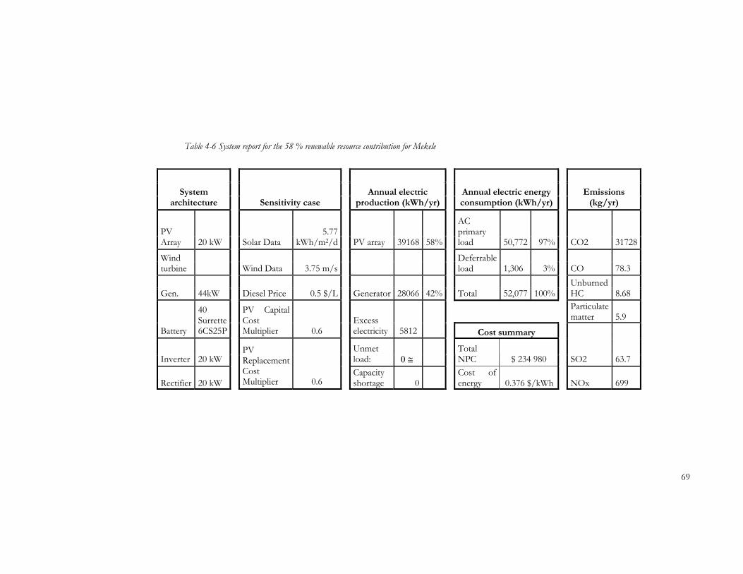
69

Table 4-6 System report for the 58 % renewable resource contribution for Mekele

System architecture Sensitivity case

Annual electric production (kWh/yr)

Annual electric energy consumption (kWh/yr)

Emissions (kg/yr)

PV Array 20 kW Solar Data

5.77 kWh/m2/d PV array 39168 58%

AC primary load 50,772 97% CO2 31728

Wind turbine Wind Data 3.75 m/s

Deferrable load 1,306 3% CO 78.3

Gen. 44kW Diesel Price 0.5 $/L Generator 28066 42% Total 52,077 100%

Unburned HC 8.68

Particulate matter 5.9

Battery

40 Surrette 6CS25P

PV Capital Cost Multiplier 0.6

Excess electricity 5812 Cost summary

Inverter 20 kW

Unmet load: 0 ≅

Total NPC $ 234 980 SO2 63.7

Rectifier 20 kW

PV Replacement Cost Multiplier 0.6

Capacity shortage 0

Cost of energy 0.376 $/kWh NOx 699

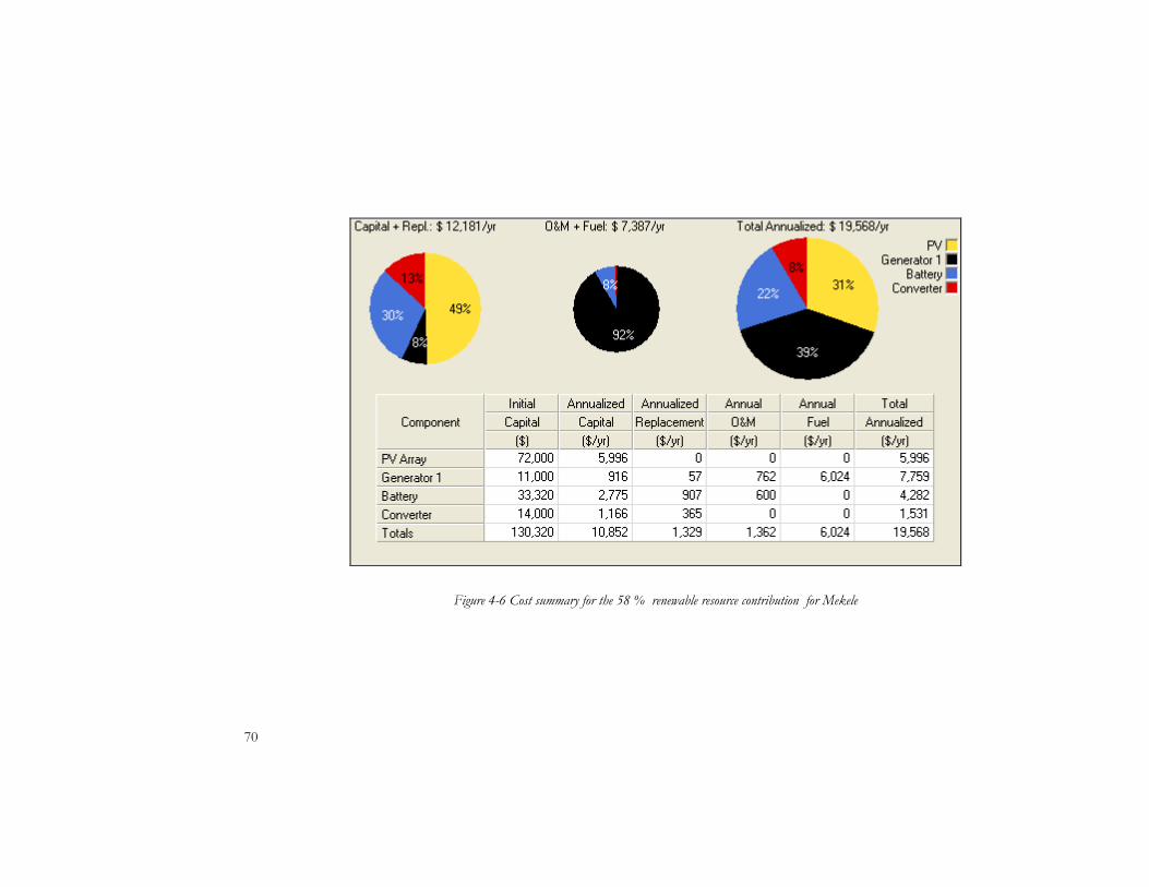
70

Figure 4-6 Cost summary for the 58 % renewable resource contribution for Mekele

71

Table 4-7 System report for the 45 % renewable resource contribution for Mekele

System architecture Sensitivity case

Annual electric production (kWh/yr)

Annual electric energy consumption (kWh/yr)

Emissions (kg/yr)

PV Array 5 kW Solar Data

5.77 kWh/m2/d PV array 9,792 16%

AC primary load 50,772 97% CO2 35,874

Wind turbine

1Generic 20kW Wind Data 3.75 m/s

Wind turbine 17,509 29%

Deferrable load 1,306 3% CO 88.5

Gen. 44kW Diesel Price 0.5 $/L Generator 33,804 55% Total 52,077 100%

Unburned HC 9.81

Particulate matter 6.68

Battery

40 Surrette 6CS25P

PV Capital Cost Multiplier 0.6

Excess electricity 2535 Cost summary

Inverter 20 kW

Unmet load: 0

Total NPC $ 246,608 SO2 72

Rectifier 20 kW

PV Replacement Cost Multiplier 0.6

Capacity shortage 0

Cost of energy 0.394 $/kWh NOx 790

72

Figure 4-7 Cost summary for the 45 % renewable resource contribution for Mekele

73

Table 4-8 System report for the 84 % renewable resource contribution for Mekele

System architecture Sensitivity case

Annual electric production (kWh/yr)

Annual electric energy consumption (kWh/yr)

Emissions (kg/yr)

PV Array 30 kW Solar Data

5.77 kWh/m2/d PV array 58,751 84%

AC primary load 50,772 97% CO2 13,682

Wind turbine Wind Data 3.75 m/s

Wind turbine

Deferrable load 1,304 3% CO 33.8

Gen. 88 kW Diesel Price 0.5 $/L Generator 11,554 16% Total 52,076 100%

Unburned HC 3.74

Particulate matter 2.55

Battery

80 Surrette 6CS25P

PV Capital Cost Multiplier 0.6

Excess electricity 2,895 Cost summary

Inverter 40 kW

Unmet load: 0

Total NPC $ 302 976 SO2 27.5

Rectifier 40 kW

PV Replacement Cost Multiplier 0.6

Capacity shortage 0

Cost of energy 0.484 $/kWh NOx 301

74

Figure 4-8 Cost summary for the 84 % renewable resource contribution for Mekele

75

Sensitivity analysis, where multiple values for a particular input variable are entered into the software for performance analysis, was also carried out and figure 4-9 shows the variation of the PV capital multiplier against diesel price for a fixed annual wind speed of 3.75 m/s and an annual solar radiation of 5.77 kWh/m2/day. In the figure the net present cost of the most cost-effective set-up for a particular set of diesel and PV prices is shown.

Figure 4-9 Sensitivity of PV cost to diesel price for Mekele with some important NPCs labeled

As can be seen in figure 4-9, the wind energy potential is low and this has been explained earlier in the study [Bekele and Palm, 2009b]. The potentials at Mekele were evaluated with respect to the wind power classification of the US Department of Energy (DOE), and have been found to be of class 1 type. Class 1 potential is generally considered to be unsuitable for wind energy development. However, average annual wind speeds of 3–4 m/s may be adequate for non grid-connected electrical and mechanical applications such as battery charging and water pumping. The current PV price is assumed to be $3600/kW and the price varies between this and the least price, $1200/kW, which assumes a future fall in price.

$321,792

$225,721

$239,917

201,609

76

4 . 3 R e s u l t s a t N a z r e t

As in the case of Mekele, the monthly average wind energy and monthly average solar energy [Bekele and Palm, 2009a,b] of Nazret were fed into the software. Figures 4-10 and 4-11 show the data which was input. The clearness index for the solar energy, which the software produced, is also indicated in figure 4-11.

After entering data for the wind and solar resources, the software was run and the resulting list of optimal combinations of realizable supply systems was obtained in both an overall form and a categorized form. The listing is arranged in the manner described for Mekele and table 4-9 shows the list which was extracted from the complete overall table which is placed in the appendix.

Figure 4-10 Nazret monthly average wind resource

Figure 4-11 Nazret monthly average solar resource

77

Table 4-9 Extracts from the overall optimization results table for Nazret

PV (k

W)

G20

win

d tu

rbin

e

Gen

erat

or (k

W)

Batte

ry

Conv

erte

r (kW

)

Disp

atch

stra

tegy

Initi

al ca

pita

l

Tota

l NPC

COE

($/k

Wh)

Rene

wab

le fr

actio

n

Dies

el (L

)

Gen

erat

or (h

rs)

44 40 20 CC $ 58,320 $ 201,609 0.322 0 18,623 1,785 20 44 40 20 LF $ 130,320 $ 235,586 0.377 0.58 12,131 1,922 5 1 44 40 20 LF $ 121,320 $ 238,266 0.381 0.51 12,381 1,832

10 1 44 40 20 LF $ 139,320 $ 245,095 0.392 0.62 10,695 1,683 10 1 44 40 40 LF $ 153,320 $ 257,109 0.411 0.63 9,894 1,428

2 44 40 20 LF $ 148,320 $ 268,212 0.429 0.61 11,275 1,658 20 1 44 40 20 LF $ 175,320 $ 270,473 0.433 0.75 9,105 1,513 10 1 44 60 40 LF $ 169,980 $ 275,732 0.441 0.65 8,883 1,249 5 2 44 40 20 LF $ 166,320 $ 276,115 0.442 0.7 9,745 1,512

30 44 40 40 LF $ 180,320 $ 278,749 0.446 0.7 10,379 1,572 30 44 60 40 LF $ 196,980 $ 280,101 0.448 0.77 7,084 1,068 20 1 44 60 40 LF $ 205,980 $ 283,955 0.454 0.84 4,766 710 10 2 44 40 20 LF $ 184,320 $ 287,106 0.459 0.76 8,672 1,412 30 44 80 40 LF $ 213,640 $ 290,993 0.465 0.83 4,940 726 10 2 44 40 40 LF $ 198,320 $ 293,861 0.47 0.79 7,083 1,044 20 1 44 60 60 LF $ 219,980 $ 302,259 0.483 0.84 4,756 706 20 1 44 80 40 LF $ 222,640 $ 302,958 0.484 0.87 3,793 557

Once again, the extract is based on the contribution made by renewable resources. Those set-ups with a renewable fraction greater than 50% are considered. It can be noted from the table that the system with the least NPC is again the non-renewable set-up. The NPC for this set-up is the same, $201 609 at a COE of 0.322 $/kWh. Despite the low cost no contribution is made by renewable resources.

The following cost effective setup is that in the second row with a renewable resource proportion of 58 % with the generator operating under Load following (LF) strategy. The NPC for this setup is $ 235,586 and the COE is 0.377$/kWh. The diesel oil used annually is 12,131 liters and the corresponding generator operation time is 1,922 hours. There is no wind turbine in this system. However, the penetration into the renewable resource is quite significant and this set up can be a good choice to implement. Figure 4-12 shows the monthly average electrical

78

production of this system. Important information about the setup is given in table 4-11. The cost breakdown supported by a pie-chart for this setup is also given in figure 4-15.

Figure 4-12 Contribution of the power units with a 58 % proportion of renewables for Nazret

One place ahead in the list, there is another PV-Wind turbine-Gen-Battery-Converter set-up, with a renewable proportion of 62 %. The NPC for this set-up is $245,095 and the COE is 0.392 $/kWh. This is also a good choice for implementation. The monthly average electricity production for this set-up is shown in figure 4-13, and table 4-12 gives important information about this set-up. Furthermore, the cost breakdown, supported by a pie-chart, is given in figure 4-16.

Another interesting set-up in the list is that in the last row, with an 87 % contribution made by renewable resources. This can be said to be an excellent proportion of renewable resources, but at the cost of a 23.6 % increase in the total NPC ($ 302,958) over the set-up with a 62 % renewable contribution ($ 245,095). However, this is once again a matter of priority, such as giving due merit to the utilization of renewable resources in view of the future benefits.

The monthly average electrical production for this set-up is given in figure 4-14. Information about the system is given in table 4-13. The cost breakdown for this set-up, supported by a pie-chart, is also given in figure 4-17.

79

Figure 4-13 Contribution of the power units with a 62 % proportion of renewables for Nazret

Figure 4-14 Contribution of the power units with an 87 % proportion of renewables for Nazret

The result in a categorized form, where only the least cost system is considered from each system type, is given in table 4-10. The first row of the table contains the same set-up as the earlier table, which was discussed previously. The two set-ups of greatest interest in this table are again those with a 100 % renewable component. One is a PV, Wind-turbine, Battery, and Converter set-up and the other comprises PV, Battery, and Converter. The NPC for the first is $ 473,123 and that for the second is $ 492,244. The corresponding COEs are 0.757 $/kWh and 0.787 $/kWh respectively.

80

Table 4-10 Optimization results in a Categorized form at Nazret; ranking is according to the NPC of each system type

PV (k

W)

G20

G

en1(

kW)

Batte

ry

Conv

erte

r(kW

)

Disp

atch

stra

tegy

Initi

al ca

pita

l

Tota

l NPC

COE

($/k

Wh)

Rene

wab

le fr

actio

n

Die

sel (

L)

Gen

1 (h

rs)

44 40 20 CC $ 58,320 $ 201,609 0.322 0 18,623 1,785 5 44 40 20 LF $ 76,320 $ 219,264 0.351 0.17 17,891 2,374 1 44 40 20 LF $ 103,320 $ 234,729 0.375 0.37 14,561 2,030

5 1 44 40 20 LF $ 121,320 $ 238,266 0.381 0.51 12,381 1,832 10 1 44 20 LF $ 106,000 $ 334,901 0.536 0.35 31,002 4,507 10 44 20 LF $ 61,000 $ 346,411 0.554 0.16 40,553 5,946

1 44 LF $ 56,000 $ 346,501 0.554 0.18 40,208 6,054 44 LF $ 11,000 $ 412,070 0.659 0 57,291 8,760

70 1 100 40 CC $ 408,300 $ 473,123 0.757 1 50 200 60 CC $ 388,600 $ 492,244 0.787 1

81

Table 4-11 System report for the 58 % renewable resource contribution for Nazret

System architecture Sensitivity case

Annual electric production (kWh/yr)

Annual electric energy consumption (kWh/yr)

Emissions (kg/yr)

PV Array 30 kW Solar Data

5.77 kWh/m2/d PV array 38,645 58%

AC primary load 50,772 97% CO2 31,945

Wind turbine Wind Data 3.75 m/s

Wind turbine

Deferrable load 1,306 3% CO 78.9

Gen. 44 kW Diesel Price 0.5 $/L Generator 28,227 42% Total 52,077 100%

Unburned HC 8.73

Particulate matter 5.94

Battery

40 Surrette 6CS25P

PV Capital Cost Multiplier 0.6

Excess electricity 5,459 Cost summary

Inverter 20 kW

Unmet load: 0

Total NPC $ 235,586 SO2 64.2

Rectifier 20 kW

PV Replacement Cost Multiplier 0.6

Capacity shortage 0

Cost of energy 0. 377 $/kWh NOx 704

82

Figure 4-15 Cost summary for the 58 % renewable resource contribution for Nazret

83

Table 4-12 System report for the 62 % renewable resource contribution for Nazret

System architecture Sensitivity case

Annual electric production (kWh/yr)

Annual electric energy consumption (kWh/yr)

Emissions (kg/yr)

PV Array 10 kW Solar Data

5.78 kWh/m2/d PV array 19,322 29%

AC primary load 50,772 97% CO2 28,361

Wind turbine

1Generic 20kW Wind Data 3.99 m/s

Wind turbine 22,018 33%

Deferrable load 1,305 3% CO 70

Gen. 44 kW Diesel Price 0.5 $/L Generator 25,212 38% Total 52,076 100%

Unburned HC 7.75

Particulate matter 5.28

Battery

40 Surrette 6CS25P

PV Capital Cost Multiplier 0.6

Excess electricity 5,994 Cost summary

Inverter 20 kW

Unmet load: 0

Total NPC $ 245,612 SO2 57

Rectifier 20 kW

PV Replacement Cost Multiplier 0.6

Capacity shortage 0

Cost of energy 0.393 $/kWh NOx 625

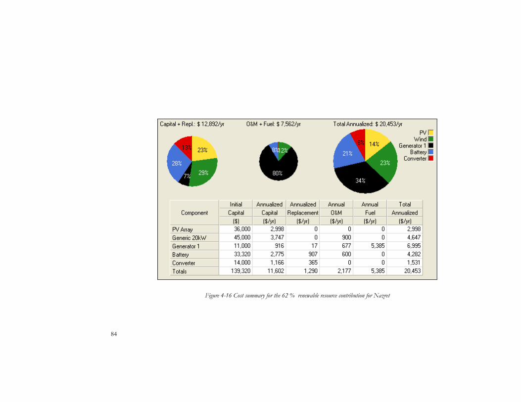
84

Figure 4-16 Cost summary for the 62 % renewable resource contribution for Nazret

85

Table 4-13 System report for the 87 % renewable resource contribution for Nazret

System architecture Sensitivity case

Annual electric production (kWh/yr)

Annual electric energy consumption (kWh/yr)

Emissions (kg/yr)

PV Array 20 kW Solar Data

5.78 kWh/m2/d PV array 38,645 55%

AC primary load 50,772 97% CO2 10,217

Wind turbine

1Generic 20kW Wind Data 3.99 m/s

Wind turbine 22,018 31%

Deferrable load 1,305 3% CO 25.2

Gen. 44 kW Diesel Price 0.5 $/L Generator 9,521 14% Total 52,076 100%

Unburned HC 2.79

Particulate matter 1.901

Battery

80 Surrette 6CS25P

PV Capital Cost Multiplier 0.6

Excess electricity 5,994 Cost summary

Inverter 40 kW

Unmet load: 0

Total NPC $ 303,538 SO2 20.5

Rectifier 40 kW

PV Replacement Cost Multiplier 0.6

Capacity shortage 0

Cost of energy 0.485 $/kWh NOx 225

86

Figure 4-17Cost summary for the 87 % renewable resource contribution for Nazret

87

Sensitivity analysis was also carried out and figure 4-18 shows the variation of PV capital cost multiplier against diesel price for a fixed average wind speed of 3.99 m/s and solar radiation of 5.8 kWh/m2/day. In the figure, the net present cost of the most cost-effective set-up for a particular set of diesel and PV prices is also included.

Figure 4-18 Sensitivity of PV cost to diesel price for Nazret with some important NPCs labeled

$318,291

$224,628 $201,609

$240,721

88

4 . 4 R e s u l t s a t D e b r e z e i t

As carried out for the previous locations, Mekele and Nazret, the monthly average wind energy [Bekele and Palm, 2009b] and monthly average solar energy of Debrezeit [Bekele and Palm, 2009a] were fed into the software. Figures 4-19 and 4-20 show the wind and solar energy potential of Debrezeit, which was input to the software. .

Figure 4-19 Debrezeit monthly average wind resource

Figure 4-20 Debrezeit monthly average solar resource

The resulting list of optimal combinations of realizable setups, obtained by running the software, is given in both overall and categorized forms. Table 4-12 shows the list extracted from the complete overall table, which is found in the appendix.

The extract from the table is again based on the contribution made by renewable resources in the realizable set-ups. The set-up in the first row

89

is the same as for the other sites. The other set-ups are selected for having a proportion of renewable resources greater than 50 %.

Table 4-14 Extracts from the overall optimization results table for Debrezeit

PV(k

W)

G20

Gen

(kW

)

Batte

ry

Conv

erte

r ( k

W)

Disp

atch

stra

tegy

Initi

al ca

pita

l

Tota

l NPC

COE

($/k

Wh)

Rene

wab

le fr

actio

n

Dies

el (L

)

Gen

erat

or (h

rs)

44 40 20 CC $ 58,320 $ 201,609 0.322 0 18623 1785 20 44 40 20 LF $ 130,320 $ 235,177 0.376 0.58 12078 1909 15 1 44 40 20 LF $ 157,320 $ 276,081 0.441 0.53 12550 1947 20 44 80 20 LF $ 163,640 $ 276,560 0.442 0.62 10617 1729 30 44 40 20 CC $ 166,320 $ 278,443 0.445 0.66 13037 2127 30 44 60 40 LF $ 196,980 $ 279,851 0.448 0.77 7048 1062 20 1 44 40 20 LF $ 175,320 $ 285,862 0.457 0.62 11339 1811 30 44 80 40 LF $ 213,640 $ 290,597 0.465 0.83 4883 716 20 1 44 60 20 LF $ 191,980 $ 305,266 0.488 0.64 10417 1701 30 44 100 40 LF $ 230,300 $310,604 0.497 0.85 4053 590

In the table the first row contains the same set-up as in the earlier tables for the other locations and it is a set-up with no contribution (0 %) made by renewable resources. The next row contains a PV-Gen-battery-Converter set-up. For just a 16.7 % increase in total NPC over the first set-up ($201,609 to $235,177), the percentage contribution made by renewables increased from 0 to 58 %. This is therefore an attractive set-up for implementation. Of course, there is no wind turbine involved in the system; the wind energy potential at this location is quite low, as can be seen from figure 4-19 and also from previous investigation [Bekele and Palm, 2009b].

Figure 4-21 shows the monthly average electrical production. Important information about the setup is also given in table 4-15. Figure 4-23 shows the cost breakdown supported by a pie-chart.

90

Figure 4-21 Contribution of the power units with a 58 % proportion of renewables for Debrezeit

The following set-up involves all the available power generating units; PV, wind turbine, generator, battery, and converter. For this set-up the total NPC is $ 276,081 but with a renewable proportion of 53 %. This is an increase in NPC of over 17 % compared to the earlier setup but a 5% decrease in the contribution made by renewable resources. Unless there is a motive for using wind energy as well, this setup shouldn't be considered as a better choice.

The maximum contribution by renewables, 85 %, is achieved by the set-up given at the end of the table. For this set-up the NPC is $310,604, which is a 32 % increase in the total NPC over the setup with a renewable contribution of 58 %. Of course, the percentage increase in the proportion of renewable resources is quite significant, 46 %. With the same arguments, set out in the previous cases, this setup can also be seen as an alternative for implementation. It should be noted that this set-up does not include a wind turbine.

The monthly average electrical production for this set-up is given in figure 4-22. Information about the system is given in table 4-16. The cost breakdown for this set-up, supported by a pie-chart, is also given in figure 4-24.

91

Figure 4-22 Contribution of the power units with an 85 % proportion of renewables for Debrezeit

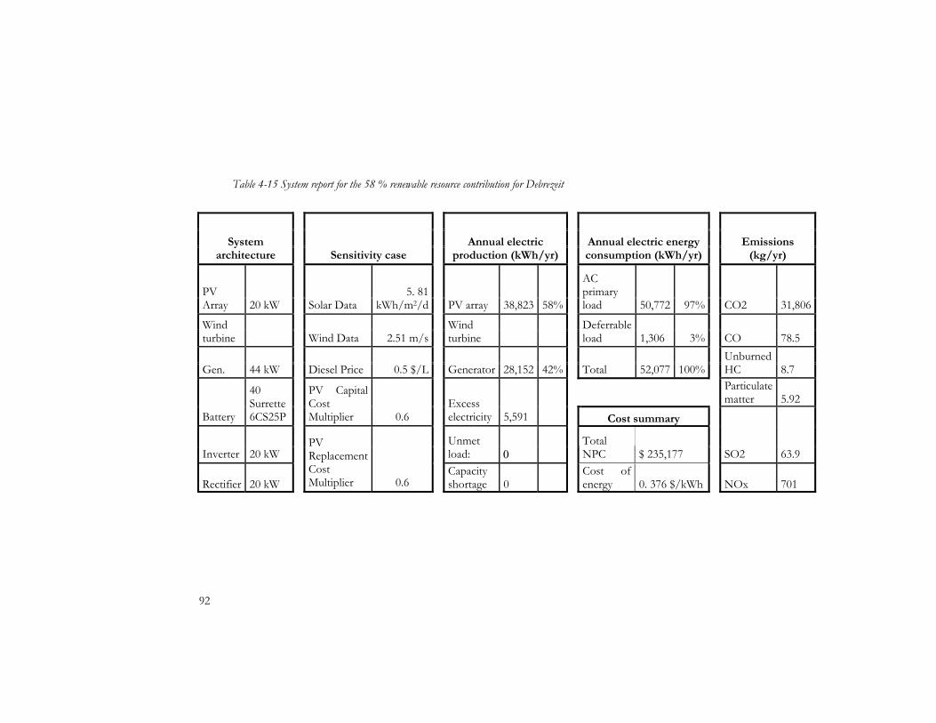
92

Table 4-15 System report for the 58 % renewable resource contribution for Debrezeit

System architecture Sensitivity case

Annual electric production (kWh/yr)

Annual electric energy consumption (kWh/yr)

Emissions (kg/yr)

PV Array 20 kW Solar Data

5. 81 kWh/m2/d PV array 38,823 58%

AC primary load 50,772 97% CO2 31,806

Wind turbine Wind Data 2.51 m/s

Wind turbine

Deferrable load 1,306 3% CO 78.5

Gen. 44 kW Diesel Price 0.5 $/L Generator 28,152 42% Total 52,077 100%

Unburned HC 8.7

Particulate matter 5.92

Battery

40 Surrette 6CS25P

PV Capital Cost Multiplier 0.6

Excess electricity 5,591 Cost summary

Inverter 20 kW

Unmet load: 0

Total NPC $ 235,177 SO2 63.9

Rectifier 20 kW

PV Replacement Cost Multiplier 0.6

Capacity shortage 0

Cost of energy 0. 376 $/kWh NOx 701

93

Figure 4-23 Cost summary for the 58 % renewable resource contribution for Debrezeit

94

Table 4-16 System report for the 85 % renewable resource contribution for Debrezeit

System architecture Sensitivity case

Annual electric production (kWh/yr)

Annual electric energy consumption (kWh/yr)

Emissions (kg/yr)

PV Array 30 kW Solar Data

5. 81 kWh/m2/d PV array 58,234 85%

AC primary load 50,772 97% CO2 10,673

Wind turbine Wind Data 2.51 m/s

Wind turbine

Deferrable load 1,304 3% CO 26.3

Gen. 44 kW Diesel Price 0.5 $/L Generator 9,981 15% Total 52,076 100%

Unburned HC 2.92

Particulate matter 1.99

Battery

100 Surrette 6CS25P

PV Capital Cost Multiplier 0.6

Excess electricity 354 Cost summary

Inverter 40 kW

Unmet load: 0

Total NPC $ 310,604 SO2 21.4

Rectifier 40 kW

PV Replacement Cost Multiplier 0.6

Capacity shortage 0

Cost of energy 0. 497 $/kWh NOx 235

95

Figure 4-24 Cost summary for the 85 % renewable resource contribution for Debrezeit

96

The results obtained in a categorized form are given in table 4-17. The set-up in the first row is again the same as those in the first row of the other tables. The two set-ups with a 100 % renewable contribution are: the set-up with PV, Battery, and Converter and the set-up with PV, Wind-turbine, Battery, and Converter. The total NPC for the first is $ 492,244 and that for the second is $ 548,052. The corresponding COEs are 0.787 $/kWh and 0.876 $/kWh respectively.

Table 4-17 Optimization results in a Categorized form; ranking is according to the NPC of each system type

PV (k

W)

G20

G

en1(

kW)

Batte

ry

Conv

erte

r (kW

) D

ispat

ch st

rate

gy

Initi

al ca

pita

l

Tota

l NPC

COE

($/k

Wh)

Rene

wab

le

frac

tion

Dies

el (L

)

Gen

1 (h

rs)

44 40 20 CC $ 58,320 $ 201,609 0.322 0 18,623 1,785 5 44 40 20 LF $ 76,320 $ 219,243 0.351 0.17 17,886 2,375 1 44 40 20 CC $ 103,320 $ 250,466 0.401 0.07 17,572 1,694

5 1 44 40 20 LF $ 121,320 $ 267,525 0.428 0.24 16,752 2,269 15 44 20 LF $ 79,000 $ 343,000 0.548 0.24 37,563 5,445 10 1 44 20 LF $ 106,000 $ 382,675 0.612 0.2 37,797 5,512

44 LF $ 11,000 $ 412,070 0.659 0 57,291 8,760 1 44 LF $ 56,000 $ 434,886 0.695 0.03 52,671 8,012

50 200 60 CC $ 388,600 $ 492,244 0.787 1 50 1 200 60 CC $ 433,600 $ 548,052 0.876 1

With a similar argument to that stated in the previous cases, these set-ups could also be considered for implementation. Otherwise, the NPC for each does indeed seem significantly high and compared to the set-up with a 58 % proportion of renewables, discussed earlier, it is again more than double.

In the sensitivity analysis, figure 4-25 shows the PV capital cost multiplier against diesel price. Here again, the net present cost of the most cost effective set-up for a particular set of diesel and PV price is shown.

97

In this figure it can be seen that the wind plays no role in the supply of energy to the community. This is understandable as the annual average wind speed at the location is just 2.51 m/s.

Figure 4-25 Sensitivity of PV cost to diesel price for Debrezeit with some important NPCs labeled

$226,202

$322,200

$201,609

$260,594

98

5 Conclusion

In simple terms what has been accomplished in this work is firstly the determination of solar and wind energy potentials at four typical locations in Ethiopia. Then, based on these potentials, a feasibility study for a standalone electric power supply system for a model community of 200 families in a village as been conducted.

In determining the wind energy potential of the sites, the study is based on relatively recent (2000 – 2003) synoptic wind data obtained from the NMSA. The data was recorded only five times a day from dawn to dusk and no data was recorded during the night. Hence, a way needed to be found to compensate for the missing night-time data and this is one of the core components of this study. The method is well explained in the published paper [Bekele and Palm, 2009b] and the authors believe that this method is of great importance to researchers working on similar issues in most developing countries, where properly recorded data is not available. A piece of software (HOMER) was used as as an aid for the study. The results obtained have been confirmed by recovering the measured daytime data to an accuracy of better than 2%.

From the results, the wind energy potential of one of the sites, Debrezeit, is considerably lower than the other three locations. However, it can be concluded that, generally-speaking, although the potential may not be sufficient for a large, independent wind energy farm, the analysis has shown that wind energy may in some cases be a viable option if integrated into other energy conversion systems such as PV, diesel generator and battery. The results of this study can be considered to be applicable to most regions in the country with similar climatic conditions.

Regarding solar energy potential, as in the case of the wind, there is no accurately measured solar radiation database. Only sunshine hour data was available. Therefore, mathematical models able to incorporate the available sunshine hour data and provide the required solar radiation data were used for determining the potential at each location. The findings were also cross-checked against satellite data obtained from other sources [NASA, 2008] and [Meteonorm, Ver. 5.1]. The results

99

demonstrated the availability of extensive utilizable solar energy at each location.

The feasibility study for the hybrid system is based on the findings of the wind and solar energy potentials at the particular locations. With the potentials determined, three different approaches have been followed in the hybrid system design. In the first approach, system components that are commonly available have been included in the design without much concern about the efficiency. This is done for both the load and the supply side. In the second approach [Bekele and Palm, 2009d] with a thorough market-survey the best technologies available are compared and those with the highest efficiency are selected. A third approach followed is to see if cost is minimized by considering a self contained system, i.e., every household having its own supply system [Bekele and Palm, 2009d]. The results obtained in the second approach have shown that the net present cost is less than 50 % of that for the first approach. The third approach is found to be of a higher cost.

In the results, numerous alternative feasible hybrid set-ups, with different levels of contribution by the renewable resources, were obtained. Despite the numerous alternatives, the choice is restricted by the varying net present cost of each set-up. Compared to the current global electricity tariff [Wikipedia, 2008] and the tariff in the country (<5 cents) where the main source of electric energy is hydro-power; the costs of the feasible set-ups obtained in this study are high, in the range of 30 to 40 cents per kilowatt hour and this is slightly worrisome. However, considering the shortage of power in the country (only 15 % coverage), its role in the protection of vegetation and forestry and therefore the prevention of soil degradation, the improvement to the quality of life of the many people residing in the countryside, the future situation regarding fossil fuel sources, and its contribution to the reduction of pollutant emissions into the environment, this cost should not be seen as a significant impairment.

It should also be noted that free solar and wind energy will also be utilized, load will be satisfied in an optimal way; help is given to the mobilization of investments towards clean energy; and, most of all, the poor will benefit from the electric light provided.

100

N o m e n c l a t u r e

A Area (m2)

Ac Array area (m2)

COE Cost of energy $/kWh

c Speed of light m/s)

c’ A scale parameter (Eq. 1-6) (m/s)

Eg Band gap energy (eV)

Ea Armature voltage (V)

Eph Photon energy

fj Frequency of occurrence in the jth class (Eq. 1-7)

G SC The solar constant =1367 (W/m2)

TG Incident solar radiation on the array (W/m2)

g Gravitational constant (m/s2)

h Planck constant

H Monthly average daily radiation on a horizontal surface (MJ/m2)

0H Monthly average daily extraterrestrial radiation on a horizontal surface (MJ/m2)

eH Mean value of the estimated radiation (MJ/m2)

obH Mean value of the obtained radiation (MJ/m2)

I Load current (A)

Ia Armature current (A)

ID Diode current (A)

Isc(G) Maximum power current (A)

ISh Shunt resistance current (A)

IL Current produced by the cell (A)

Imp Maximum power point (A)

Io Reverse saturation current of diode (A)

jXs Synchronous reactance (Ω)

101

K Boltzmann's constant

k A constant known as shape factor(Eq. 1-6)

M Number of data points (Eq. 2-7)

m Diode quality factor

N Number of photons

NPC Net present cost ($)

n Monthly average daily number of hours of bright sunshine

n Number of wind speed readings (Eq. 1-2)

ns Synchronous speed (RPM)

P Power (W)

Po Standard sea level atmospheric pressure (Pa)

pl Number of pole pairs

Pmp Maximum power point (W)

pr Pressure (Pa)

Po Standard sea level atmospheric pressure (Pa)

q Charge on an electron (C)

R Specific gas constant (Jkg-1 K-1)

Ra Armature winding resistance (Ω)

T Temperature (0K)

u Wind velocity (m/s)

u Mean wind speed (m/s)

uj The jth wind speed (m/s)

V Output voltage (V)

Va Terminal voltage (V)

Vj Median velocity in class j (m/s)

Vmp Maximum power voltage (V)

Voc Open circuit voltage (V)

z Region’s elevation (m)

z0 Roughness length (Eq. 1-9) (m)

102

zr Reference height (Eq. 1-9) (m)

Greek alphabets

δ Declination angle

φ Latitude angle

λ The wavelength of light (m/s)

mpη Maximum power point efficiency (Eq. 3-5)

eη Efficiency of power conditioning equipment (Eq. 3-5)

ρ Density of the air kg/m3

ρj The jth readings of the air density kg/m3

uσ Standard deviation of wind speed m/s

ω The sunset hour angle

103

R e f e r e n c e s

Bekele G, Palm B., 2009a, Assessment of Solar Energy Potential at Four Typical Locations in Ethiopia, submitted to the journal Energy for Sustainable Development

Bekele G, Palm B. 2009b, Wind energy potential assessment at four typical locations in Ethiopia, Applied Energy, 86: 388–396

Bekele, G. Palm B., 2009c, Feasibility Study for a Standalone Solar-Wind Hybrid Energy System for Application in Ethiopia, Applied Energy, 86: 487–495.

Bekele, G. Palm B., 2009d, Solar-Wind-Based Village Electrification In Ethiopia: A Comparison Of Technologies, submitted to the journal Renewable Energy.

CIA The world fact book, 2008, http://www.umsl.edu/services/govdocs/wofact2007/geos/et.html#People

Danish Wind Industry Association (Dec. 2008) http://www.windpower.org/en/tour/wres/index.htm

Digitimes Bits+Chips, (April, 2009) http://www.digitimes.com/news/a20090408PD201.html

Drake F, Mulugetta Y. 1996, Assessment of solar and wind energy resources in Ethiopia: Part 2. Wind energy, Solar Energy, 51: 205-217

Duffie JA, Beckman WA., 1991, Solar Engineering of Thermal Processes, 3rd Edn. Wiley, New York

Ethiopian National Energy Committee (ENEC) (1986) Co-Operation Agreement in the Energy Sector between ENEC and CESEN-ANSALDO/FINMECCANICA Group. Final Report, Solar Energy Resources, Addis Ababa.

104

EEPCo, Ethiopian Electric Power Corporation, 2007 http://www.eepco.gov.et/psdp_home.html, http://wind4africa.net/news/EEPCO.pdf http://www.eepco.gov.et/brief.html

Gasch R, Twele J., 2002, Wind Power Plants, Fundamentals, Design, Construction and Operation, Solarpraxis AG

Generator Power, 2009, http://www.generatorpower.com.au/faq.php

Genesis Photography, 2009 http://genesisphotography.files.wordpress.com/2008/05/ethiopia-map1.jpg,

Gipe P., 1999, Wind Energy Basics, a Guide to Small and Micro Wind Systems; Chelsea Green publishing company

Google map, March 2009, http://maps.google.com/maps?hl=en&q=map+of+Ethiopia&um=1&ie=UTF-8&split=0&ei=kwzfSYPMINeMsAagoaTaCA&sa=X&oi=geocode_result&ct=image&resnum=1

Greenpeace International, Feb 2007, http://www.greenpeace.org.

GTZ Deutsche Gesellschaft für Technische Zusammenarbeit GmbH, April 2005, Wind Energy Programme TERNA Site Selection Report: Ethiopia

HOMER, the micropower optimization model; Ver. 2.19 http://www.nrel.gov/homer; Feb 2006

Himri Y, et al, 2008, Techno-economical study of hybrid power system for a remote village in Algeria, Energy 33, 1128–1136

Iowa Energy Centre, July 2008, http://www.energy.iastate.edu/renewable/wind/wem/economic_issues.htm

105

Joliet Wind turbines, Dec. 2008, http://www.joliet-wind-turbines.com/cyclone_20kw_wind_turbine.html

Lambrecht, 2009, http://www.gabcors.com/catalog/lambrechteng/products/001_wind/011-14670-e.pdf

Layi Fagbenle R., 1993, Total Solar Radiation Estimates in Nigeria Using a Maximum-Likelihood Quadratic Fit, Renewable Energy, 3: 813-17

Magda Moner-Girona, 2009, A new tailored scheme for the support of renewable energies in developing countries Energy Policy 37, 2037–2041

Manwell J.F., McGowan, J.G., Rogers, A.L., 2002, Wind Energy Explained, Theory, Design and Application, Wiley, UK

Meteonorm, Ver-5.1x, Global Meteorological Database for Solar Energy and Applied Meteorology

Miodrag Zlatanovic, 2009 http://www.ewec2008proceedings.info/ewec2008/allfiles2/459_EWEC2008fullpaper.pdf

Mulugetta Y, Drake F., 1996, Assessment of solar and wind energy in Ethiopia. I. Solar energy, Solar Energy, 57, 205-17

Nfah EM, et al, 2008, Simulation of off-grid generation options for remote villages in Cameroon, Renewable Energy 33, 1064-1072

Nfah EM et al, 2008, Modelling of solar/diesel/battery hybrid power systems for far-north Cameroon, Renewable Energy 32, 832–844

Nfah EM, Ngundam, 2008, Modelling of wind/Diesel/battery hybrid power systems for far North Cameroon, Energy Conversion and Management 49 (2008) 1295–1301

106

NASA Atmospheric Science Data Centre (Dec. 2008) http://eosweb.larc.nasa.gov/sse/

Nguyen BT, Pryor TL., 1997, The Relationship between Global Solar Radiation and Sunshine Duration in Vietnam, Renewable Energy, 2: 47-60

Oklahoma Windpower Tutorial, Dec. 2008, http://www.seic.okstate.edu/owpi_old/about/Library/Lesson3_WPD_windclass.pdf

Rietveld MR., 1978, A New Method For Estimating The Regression Coefficients In The Formula Relating Solar Radiation To Sunshine, Agricultural Meteorology; 19: 243-52

Safari B, 2009, A review of energy in Rwanda, Available online Renewable and Sustainable Energy Reviews

Shaahid SM, Elhadidy MA., 2007, Technical and Economic Assessment of Grid-independent Hybrid photovoltaic–diesel–battery Power Systems for Commercial Loads in Desert Environments, Renewable and Sustainable Energy Reviews, 11: 1794-810

Solar Buzz, (April 2009), http://www.solarbuzz.com/Moduleprices.htm

Soler A., 1990, Statistical comparison for 77 European stations of 7 sunshine-based models, Solar Energy, 45: 365-70

Tomas Markvart, Solar Electricity, 2000, 2nd Edn. Wiley, England

Turton SM., 1987, The Relationship between Total Irradiation and Sunshine Duration in the Humid Tropics, Solar energy; 38: 353-54

Vining R, Gregory J., Oct 2007, Daily Wind Patterns: Understanding of processes. Proceedings from Wind Erosion: An International Symposium/Workshop, Kansas State University, June 1997, http://www.weru.ksu.edu/symposium/proceedings/vining.pdf

107

Weatherbase , Feb 2006, http://www.weatherbase.com/weather/weatherall.php3?s=005436&refer=&units=us

Wikipedia, Dec. 2008, http://en.wikipedia.org/wiki/Electricity_tariff

Wolde-Ghiorgis W., 1988, Wind energy survey in Ethiopia, Solar Wind Technology; 5: 341-351

108

Appendix A:

Overal l Optimization Results Tables

Table 5-1 Overall optimization results table for Addis Ababa

PV(k

W)

G20

G

en (k

W)

Batte

ry

Conv

erte

r ( k

W)

Disp

atch

stra

tegy

Initi

al ca

pita

l

Tota

l NPC

COE

($/k

Wh)

Rene

wab

le fr

actio

n

Die

sel (

L)

Gen

erat

or (h

rs)

44 40 20 CC $ 58,320 $ 201,609 0.322 0 18,623 1,785 5 44 40 20 LF $ 76,320 $ 220,728 0.353 0.16 18,115 2,391 44 40 20 LF $ 58,320 $ 222,616 0.356 0 21,056 2,725

10 44 40 20 LF $ 94,320 $ 226,668 0.362 0.3 16,217 2,293 44 60 20 CC $ 74,980 $ 227,227 0.363 0 18,605 1,788

5 44 60 20 CC $ 92,980 $ 230,456 0.369 0.15 16,320 1,638 15 44 40 20 LF $ 112,320 $ 231,855 0.371 0.43 14,260 2,137

1 44 40 20 LF $ 103,320 $ 233,435 0.373 0.39 14,355 2,021 5 44 40 40 LF $ 90,320 $ 238,842 0.382 0.16 18,083 2,379 5 1 44 40 20 LF $ 121,320 $ 239,756 0.383 0.51 12,599 1,858

20 44 40 20 LF $ 130,320 $ 240,104 0.384 0.54 12,815 1,981 10 44 40 40 LF $ 108,320 $ 240,814 0.385 0.3 15,726 2,104

44 40 40 LF $ 72,320 $ 241,008 0.386 0 21,057 2,725 15 44 40 40 LF $ 126,320 $ 245,888 0.393 0.43 13,780 1,924 5 44 60 20 LF $ 92,980 $ 246,224 0.394 0.16 18,084 2,387 44 40 40 CC $ 72,320 $ 247,995 0.397 0 22,461 2,508 44 60 20 LF $ 74,980 $ 248,124 0.397 0 21,027 2,721

10 1 44 40 20 LF $ 139,320 $ 248,587 0.398 0.61 11,214 1,736

109

1 44 40 40 LF $ 117,320 $ 248,751 0.398 0.4 13,987 1,897 88 40 20 CC $ 69,320 $ 249,872 0.4 0 23,503 1,712

10 44 60 20 LF $ 110,980 $ 252,225 0.403 0.3 16,194 2,291 5 88 40 20 CC $ 87,320 $ 252,616 0.404 0.15 21,112 1,648 5 1 44 40 40 LF $ 135,320 $ 252,697 0.404 0.52 11,931 1,654 44 80 20 CC $ 91,640 $ 253,015 0.405 0 18,619 1,787

20 44 40 40 LF $ 144,320 $ 255,595 0.409 0.53 12,537 1,805 15 44 60 20 LF $ 128,980 $ 255,715 0.409 0.44 13,989 2,105 5 44 80 20 CC $ 109,640 $ 256,104 0.41 0.15 16,315 1,634 5 44 40 60 LF $ 104,320 $ 257,228 0.411 0.16 18,083 2,379 1 44 60 20 LF $ 119,980 $ 257,499 0.412 0.4 14,109 1,997

5 88 40 20 LF $ 87,320 $ 257,829 0.412 0.15 21,601 1,810 20 44 60 20 LF $ 146,980 $ 258,016 0.413 0.56 11,679 1,841

1 44 60 20 CC $ 119,980 $ 258,420 0.413 0.35 14,793 1,529 10 44 40 60 LF $ 122,320 $ 259,155 0.414 0.3 15,721 2,102

44 40 60 LF $ 86,320 $ 259,394 0.415 0 21,057 2,725 10 1 44 40 40 LF $ 153,320 $ 259,616 0.415 0.62 10,271 1,470 5 44 40 20 CC $ 76,320 $ 259,965 0.416 0.14 23,348 3,550

15 1 44 40 20 LF $ 157,320 $ 260,371 0.416 0.68 10,288 1,643 10 88 40 20 LF $ 105,320 $ 260,442 0.416 0.29 19,446 1,636 10 44 40 20 CC $ 94,320 $ 261,755 0.419 0.26 20,956 3,289

1 44 40 20 CC $ 103,320 $ 262,600 0.42 0.35 18,327 2,810 5 1 44 60 20 LF $ 137,980 $ 262,614 0.42 0.52 12,176 1,813

15 44 40 20 CC $ 112,320 $ 262,902 0.42 0.38 18,524 2,951 15 44 40 60 LF $ 140,320 $ 264,160 0.422 0.43 13,767 1,919 5 44 60 40 LF $ 106,980 $ 264,322 0.423 0.16 18,051 2,374 44 40 60 CC $ 86,320 $ 266,036 0.425 0 22,417 2,496

10 88 40 20 CC $ 105,320 $ 266,165 0.426 0.27 20,366 1,650 10 44 60 40 LF $ 124,980 $ 266,210 0.426 0.3 15,684 2,095 30 44 40 20 LF $ 166,320 $ 266,410 0.426 0.67 11,390 1,818

44 60 40 LF $ 88,980 $ 266,521 0.426 0 21,029 2,721 20 44 40 20 CC $ 130,320 $ 266,677 0.426 0.48 16,486 2,650 5 1 44 40 20 CC $ 121,320 $ 266,760 0.427 0.46 16,274 2,582 1 44 40 60 LF $ 131,320 $ 267,114 0.427 0.4 13,985 1,896

10 1 44 40 20 CC $ 139,320 $ 267,141 0.427 0.56 13,752 2,215 2 44 40 20 LF $ 148,320 $ 267,956 0.428 0.63 11,228 1,662

15 44 60 40 LF $ 142,980 $ 268,208 0.429 0.44 13,340 1,817 15 1 44 40 40 LF $ 171,320 $ 268,568 0.429 0.7 8,917 1,309 20 44 60 20 CC $ 146,980 $ 269,487 0.431 0.53 13,308 2,085 15 44 60 20 CC $ 128,980 $ 270,116 0.432 0.41 16,007 2,441 5 1 44 40 60 LF $ 149,320 $ 271,037 0.433 0.52 11,925 1,652 88 60 20 CC $ 85,980 $ 271,307 0.434 0 22,958 1,641

20 44 60 40 LF $ 160,980 $ 271,430 0.434 0.56 11,160 1,572

110

10 1 44 60 20 LF $ 155,980 $ 271,629 0.434 0.62 10,821 1,692 5 44 80 20 LF $ 109,640 $ 271,775 0.435 0.16 18,060 2,385 1 44 60 40 LF $ 133,980 $ 272,233 0.435 0.4 13,683 1,840

15 1 44 40 20 CC $ 157,320 $ 273,502 0.437 0.64 12,093 1,971 15 88 40 40 LF $ 137,320 $ 273,506 0.437 0.42 16,117 1,351

44 80 20 LF $ 91,640 $ 273,732 0.438 0 21,010 2,721 5 1 44 60 40 LF $ 151,980 $ 273,798 0.438 0.53 11,280 1,544

20 44 40 60 LF $ 158,320 $ 273,844 0.438 0.53 12,522 1,799 10 44 60 20 CC $ 110,980 $ 274,101 0.438 0.27 19,217 2,849

1 88 40 20 LF $ 114,320 $ 275,047 0.44 0.36 18,718 1,572 20 1 44 40 20 LF $ 175,320 $ 275,203 0.44 0.72 9,819 1,591 10 88 40 40 LF $ 119,320 $ 275,300 0.44 0.29 18,968 1,587 5 44 40 80 LF $ 118,320 $ 275,614 0.441 0.16 18,083 2,379

20 88 40 40 LF $ 155,320 $ 277,117 0.443 0.53 14,046 1,179 1 88 40 20 CC $ 114,320 $ 277,293 0.443 0.34 19,195 1,517

10 44 40 80 LF $ 136,320 $ 277,541 0.444 0.3 15,721 2,102 5 88 60 20 CC $ 103,980 $ 277,605 0.444 0.15 21,033 1,631

10 1 44 60 40 LF $ 169,980 $ 277,664 0.444 0.64 9,176 1,279 10 44 80 20 LF $ 127,640 $ 277,718 0.444 0.3 16,163 2,287

44 40 80 LF $ 100,320 $ 277,780 0.444 0 21,057 2,725 15 88 40 20 LF $ 123,320 $ 277,952 0.444 0.38 19,376 1,631 10 1 44 40 60 LF $ 167,320 $ 277,981 0.445 0.62 10,269 1,469 5 2 44 40 20 LF $ 166,320 $ 278,329 0.445 0.7 10,075 1,553 5 1 44 60 20 CC $ 137,980 $ 278,729 0.446 0.48 14,411 2,203 44 100 20 CC $ 108,300 $ 278,746 0.446 0 18,628 1,782

5 1 88 40 40 LF $ 146,320 $ 279,636 0.447 0.51 14,149 1,187 5 88 40 40 LF $ 101,320 $ 279,989 0.448 0.15 22,137 1,850 2 44 40 40 LF $ 162,320 $ 280,122 0.448 0.64 10,408 1,449

5 88 60 20 LF $ 103,980 $ 280,643 0.449 0.16 21,196 1,777 20 1 44 40 40 LF $ 189,320 $ 281,170 0.45 0.75 8,105 1,216 15 44 80 20 LF $ 145,640 $ 281,214 0.45 0.44 13,959 2,101

88 40 20 LF $ 69,320 $ 281,406 0.45 0 27,444 2,281 5 44 60 40 CC $ 106,980 $ 281,470 0.45 0.13 20,931 2,353

30 44 40 40 LF $ 180,320 $ 281,673 0.45 0.66 11,043 1,640 1 88 40 40 LF $ 128,320 $ 281,721 0.451 0.38 17,041 1,427

10 1 44 60 20 CC $ 155,980 $ 281,784 0.451 0.59 12,245 1,922 5 44 100 20 CC $ 126,300 $ 281,787 0.451 0.15 16,312 1,633

10 1 88 40 40 LF $ 164,320 $ 282,000 0.451 0.61 11,901 999 1 44 80 20 LF $ 136,640 $ 282,431 0.452 0.4 13,995 1,984

15 44 40 80 LF $ 154,320 $ 282,546 0.452 0.43 13,767 1,919 20 44 80 20 LF $ 163,640 $ 282,557 0.452 0.57 11,508 1,821 15 88 40 20 CC $ 123,320 $ 282,616 0.452 0.37 20,125 1,643 15 1 44 60 40 LF $ 187,980 $ 282,681 0.452 0.73 7,252 1,027

111

5 44 60 60 LF $ 120,980 $ 282,708 0.452 0.16 18,051 2,374 5 44 40 40 CC $ 90,320 $ 282,881 0.452 0.13 24,086 3,564 1 44 80 20 CC $ 136,640 $ 283,686 0.454 0.35 14,739 1,508

15 1 44 60 20 LF $ 173,980 $ 283,799 0.454 0.69 9,956 1,602 44 60 40 CC $ 88,980 $ 283,880 0.454 0 23,972 2,674

30 44 60 20 LF $ 182,980 $ 284,412 0.455 0.69 10,265 1,682 44 40 80 CC $ 100,320 $ 284,422 0.455 0 22,417 2,496

10 44 60 60 LF $ 138,980 $ 284,551 0.455 0.3 15,679 2,093 30 44 40 20 CC $ 166,320 $ 284,618 0.455 0.62 13,922 2,253

44 60 60 LF $ 102,980 $ 284,907 0.456 0 21,029 2,721 10 44 40 40 CC $ 108,320 $ 284,939 0.456 0.25 21,743 3,265

1 44 40 80 LF $ 145,320 $ 285,500 0.457 0.4 13,985 1,896 10 88 60 20 LF $ 121,980 $ 285,661 0.457 0.29 19,376 1,631 20 1 44 40 20 CC $ 175,320 $ 285,860 0.457 0.7 11,297 1,847 15 44 60 60 LF $ 156,980 $ 286,526 0.458 0.44 13,332 1,814 5 1 88 40 20 LF $ 132,320 $ 286,784 0.459 0.45 17,812 1,499

15 1 44 40 60 LF $ 185,320 $ 286,911 0.459 0.7 8,911 1,307 5 1 44 80 20 LF $ 154,640 $ 287,191 0.459 0.53 12,011 1,793

30 44 60 40 LF $ 196,980 $ 287,613 0.46 0.72 8,204 1,207 1 44 40 40 CC $ 117,320 $ 287,632 0.46 0.33 19,367 2,871

5 2 44 40 40 LF $ 180,320 $ 287,708 0.46 0.72 8,851 1,261 15 1 88 40 40 LF $ 182,320 $ 288,248 0.461 0.69 10,210 858 15 1 44 60 20 CC $ 173,980 $ 288,870 0.462 0.67 10,674 1,710 20 44 80 20 CC $ 163,640 $ 288,913 0.462 0.55 12,432 1,937 5 1 44 40 80 LF $ 163,320 $ 289,424 0.463 0.52 11,925 1,652 2 44 60 20 LF $ 164,980 $ 289,485 0.463 0.65 10,608 1,597

20 44 60 60 LF $ 174,980 $ 289,665 0.463 0.56 11,141 1,565 5 44 80 40 LF $ 123,640 $ 289,811 0.463 0.16 18,020 2,369

20 1 44 60 40 LF $ 205,980 $ 289,942 0.464 0.81 5,662 817 10 2 44 40 20 LF $ 184,320 $ 290,411 0.464 0.75 9,177 1,460

1 44 60 60 LF $ 147,980 $ 290,573 0.465 0.4 13,677 1,838 5 1 88 40 20 CC $ 132,320 $ 290,945 0.465 0.43 18,492 1,506 2 44 40 20 CC $ 148,320 $ 291,043 0.465 0.58 14,401 2,244

5 1 44 40 40 CC $ 135,320 $ 291,252 0.466 0.44 17,253 2,616 10 88 60 20 CC $ 121,980 $ 291,371 0.466 0.27 20,325 1,632 10 44 80 40 LF $ 141,640 $ 291,693 0.466 0.3 15,652 2,090 30 44 60 20 CC $ 182,980 $ 291,747 0.467 0.67 11,323 1,822 15 88 40 60 LF $ 151,320 $ 291,893 0.467 0.42 16,118 1,351

44 80 40 LF $ 105,640 $ 291,983 0.467 0 20,994 2,715 15 44 80 20 CC $ 145,640 $ 292,009 0.467 0.41 15,512 2,316 5 1 44 60 60 LF $ 165,980 $ 292,119 0.467 0.53 11,272 1,541

20 44 40 80 LF $ 172,320 $ 292,230 0.467 0.53 12,522 1,799 20 88 60 40 LF $ 171,980 $ 293,210 0.469 0.55 12,664 1,063

112

15 44 80 40 LF $ 159,640 $ 293,673 0.47 0.44 13,307 1,811 10 88 40 60 LF $ 133,320 $ 293,686 0.47 0.29 18,968 1,587 5 44 40 100 LF $ 132,320 $ 294,000 0.47 0.16 18,083 2,379

10 44 80 20 CC $ 127,640 $ 294,077 0.47 0.27 18,515 2,620 15 88 60 40 LF $ 153,980 $ 295,110 0.472 0.43 15,528 1,301 20 88 40 60 LF $ 169,320 $ 295,505 0.473 0.53 14,046 1,179

1 44 60 40 CC $ 133,980 $ 295,533 0.473 0.34 17,197 2,158 88 60 20 LF $ 85,980 $ 295,644 0.473 0 25,829 2,151

20 44 80 40 LF $ 177,640 $ 295,651 0.473 0.56 10,952 1,530 20 88 40 20 LF $ 141,320 $ 295,867 0.473 0.45 19,364 1,630 10 44 40 100 LF $ 150,320 $ 295,927 0.473 0.3 15,721 2,102 10 1 44 60 60 LF $ 183,980 $ 296,028 0.473 0.64 9,173 1,278

44 40 100 LF $ 114,320 $ 296,166 0.474 0 21,057 2,725 10 1 44 80 20 LF $ 172,640 $ 296,256 0.474 0.62 10,664 1,673 10 44 60 40 CC $ 124,980 $ 296,275 0.474 0.25 20,088 2,631 10 1 44 40 80 LF $ 181,320 $ 296,367 0.474 0.62 10,269 1,469

88 80 20 CC $ 102,640 $ 296,603 0.474 0 22,913 1,631 5 2 44 40 20 CC $ 166,320 $ 296,731 0.474 0.66 12,599 2,026 2 44 60 40 LF $ 178,980 $ 296,853 0.475 0.67 9,102 1,248

10 2 44 40 40 LF $ 198,320 $ 297,172 0.475 0.78 7,574 1,108 5 44 100 20 LF $ 126,300 $ 297,333 0.475 0.16 18,037 2,383 1 44 80 40 LF $ 150,640 $ 297,352 0.475 0.4 13,602 1,825

10 1 44 40 40 CC $ 153,320 $ 297,726 0.476 0.53 15,415 2,394 10 88 60 40 LF $ 135,980 $ 297,896 0.476 0.3 18,520 1,550 5 1 88 40 60 LF $ 160,320 $ 298,188 0.477 0.51 14,173 1,189 5 1 44 80 20 CC $ 154,640 $ 298,262 0.477 0.49 13,588 2,024 5 88 40 60 LF $ 115,320 $ 298,375 0.477 0.15 22,137 1,850

20 1 44 60 20 LF $ 191,980 $ 298,383 0.477 0.73 9,443 1,544 2 44 40 60 LF $ 176,320 $ 298,508 0.477 0.64 10,408 1,449

5 1 44 80 40 LF $ 168,640 $ 298,599 0.477 0.53 11,148 1,523 5 1 44 60 40 CC $ 151,980 $ 298,713 0.478 0.46 14,919 1,992

10 1 88 60 40 LF $ 180,980 $ 298,816 0.478 0.63 10,622 892 5 1 88 60 40 LF $ 162,980 $ 298,896 0.478 0.52 13,221 1,110 1 88 60 20 LF $ 130,980 $ 299,038 0.478 0.36 18,471 1,551 44 100 20 LF $ 108,300 $ 299,284 0.479 0 20,986 2,719

30 88 40 40 LF $ 191,320 $ 299,391 0.479 0.66 12,072 1,014 20 1 44 40 60 LF $ 203,320 $ 299,591 0.479 0.75 8,111 1,216 20 88 40 20 CC $ 141,320 $ 299,837 0.479 0.44 20,009 1,637 30 44 40 60 LF $ 194,320 $ 299,967 0.48 0.66 11,033 1,636 20 1 88 40 40 LF $ 200,320 $ 300,009 0.48 0.74 9,312 783

1 88 40 60 LF $ 142,320 $ 300,107 0.48 0.38 17,041 1,427 10 1 88 40 60 LF $ 178,320 $ 300,303 0.48 0.61 11,889 998 5 2 44 60 20 LF $ 182,980 $ 300,481 0.481 0.71 9,542 1,490

113

15 1 88 60 40 LF $ 198,980 $ 300,620 0.481 0.73 8,295 696 5 44 60 60 CC $ 120,980 $ 300,645 0.481 0.13 21,036 2,376

30 44 80 40 LF $ 213,640 $ 300,698 0.481 0.77 6,379 914 10 1 44 80 40 LF $ 186,640 $ 300,866 0.481 0.65 8,812 1,222

44 80 40 CC $ 105,640 $ 300,887 0.481 0 23,005 2,243 88 40 40 LF $ 83,320 $ 300,892 0.481 0 27,598 2,294

15 44 40 100 LF $ 168,320 $ 300,932 0.481 0.43 13,767 1,919 15 1 44 60 60 LF $ 201,980 $ 300,959 0.481 0.73 7,239 1,022 5 44 60 80 LF $ 134,980 $ 301,094 0.481 0.16 18,051 2,374 5 44 40 60 CC $ 104,320 $ 301,644 0.482 0.13 24,133 3,577

114

Table 5-2 Overall optimization results table for Mekele

PV(k

W)

G20

G

en (k

W)

Batte

ry

Conv

erte

r ( k

W)

Disp

atch

stra

tegy

Initi

al ca

pita

l

Tota

l NPC

COE

($/k

Wh)

Rene

wab

le fr

actio

n

Die

sel (

L)

Gen

erat

or (h

rs)

44 40 20 CC $ 58,320 $ 201,609 0.322 0 18,623 1,785 5 44 40 20 LF $ 76,320 $ 219,157 0.35 0.17 17,872 2,375 44 40 20 LF $ 58,320 $ 222,616 0.356 0 21,056 2,725

10 44 40 20 LF $ 94,320 $ 223,862 0.358 0.33 15,777 2,269 44 60 20 CC $ 74,980 $ 227,227 0.363 0 18,605 1,788

20 44 40 20 LF $ 130,320 $ 234,980 0.376 0.58 12,049 1,906 10 44 40 40 LF $ 108,320 $ 237,301 0.379 0.33 15,203 2,050 5 44 40 40 LF $ 90,320 $ 237,323 0.38 0.17 17,846 2,365 1 44 40 20 CC $ 103,320 $ 237,336 0.38 0.28 15,520 1,574 44 40 40 LF $ 72,320 $ 241,008 0.386 0 21,057 2,725 1 44 40 20 LF $ 103,320 $ 242,962 0.389 0.3 15,799 2,146

5 44 60 20 LF $ 92,980 $ 244,680 0.391 0.17 17,844 2,372 5 1 44 40 20 LF $ 121,320 $ 245,448 0.392 0.45 13,467 1,927 44 40 40 CC $ 72,320 $ 247,995 0.397 0 22,461 2,508 44 60 20 LF $ 74,980 $ 248,124 0.397 0 21,027 2,721

10 44 60 20 LF $ 110,980 $ 249,382 0.399 0.33 15,749 2,266 88 40 20 CC $ 69,320 $ 249,872 0.4 0 23,503 1,712

20 44 40 40 LF $ 144,320 $ 250,763 0.401 0.57 11,817 1,733 5 88 40 20 CC $ 87,320 $ 251,474 0.402 0.17 20,934 1,643

20 44 60 20 LF $ 146,980 $ 251,496 0.402 0.61 10,716 1,736 10 1 44 40 20 LF $ 139,320 $ 252,681 0.404 0.57 11,820 1,801

44 80 20 CC $ 91,640 $ 253,015 0.405 0 18,619 1,787 5 88 40 20 LF $ 87,320 $ 253,746 0.406 0.17 21,026 1,765 5 44 80 20 CC $ 109,640 $ 255,382 0.408 0.17 16,185 1,642

10 44 40 60 LF $ 122,320 $ 255,619 0.409 0.33 15,195 2,047 5 44 40 60 LF $ 104,320 $ 255,709 0.409 0.17 17,846 2,365 5 44 40 20 CC $ 76,320 $ 258,890 0.414 0.15 23,166 3,552

44 40 60 LF $ 86,320 $ 259,394 0.415 0 21,057 2,725 1 44 40 40 LF $ 117,320 $ 259,584 0.415 0.3 15,591 2,071

10 44 40 20 CC $ 94,320 $ 259,643 0.415 0.29 20,628 3,269

115

20 44 60 20 CC $ 146,980 $ 259,829 0.415 0.59 11,900 1,911 10 88 40 20 LF $ 105,320 $ 259,953 0.416 0.31 19,377 1,631 20 44 40 20 CC $ 130,320 $ 260,439 0.416 0.52 15,573 2,536 5 1 44 40 40 LF $ 135,320 $ 260,735 0.417 0.45 13,109 1,791

30 44 40 20 LF $ 166,320 $ 261,958 0.419 0.71 10,731 1,747 1 44 60 20 CC $ 119,980 $ 262,150 0.419 0.28 15,418 1,525

10 44 60 40 LF $ 124,980 $ 262,646 0.42 0.33 15,155 2,039 5 44 60 40 LF $ 106,980 $ 262,801 0.42 0.17 17,813 2,360

20 44 60 40 LF $ 160,980 $ 264,117 0.422 0.61 10,072 1,434 10 1 44 40 40 LF $ 153,320 $ 264,201 0.422 0.57 10,966 1,543 10 88 40 20 CC $ 105,320 $ 265,056 0.424 0.3 20,193 1,645

44 40 60 CC $ 86,320 $ 266,036 0.425 0 22,417 2,496 44 60 40 LF $ 88,980 $ 266,521 0.426 0 21,029 2,721 1 44 60 20 LF $ 119,980 $ 267,569 0.428 0.3 15,635 2,129

10 44 60 20 CC $ 110,980 $ 268,547 0.429 0.3 18,412 2,740 20 44 40 60 LF $ 158,320 $ 269,011 0.43 0.57 11,801 1,727

5 1 44 60 20 LF $ 137,980 $ 269,552 0.431 0.45 13,225 1,905 20 88 40 40 LF $ 155,320 $ 269,739 0.431 0.58 12,983 1,091 5 44 80 20 LF $ 109,640 $ 270,232 0.432 0.17 17,820 2,370

10 88 40 40 LF $ 119,320 $ 270,320 0.432 0.32 18,248 1,529 88 60 20 CC $ 85,980 $ 271,307 0.434 0 22,958 1,641

5 44 60 20 CC $ 92,980 $ 271,640 0.434 0.15 21,567 3,068 1 44 40 40 CC $ 117,320 $ 273,424 0.437 0.26 17,920 2,050

5 1 44 40 20 CC $ 121,320 $ 273,729 0.438 0.4 17,278 2,723 44 80 20 LF $ 91,640 $ 273,732 0.438 0 21,010 2,721

10 1 44 40 20 CC $ 139,320 $ 273,820 0.438 0.52 14,695 2,364 10 44 40 80 LF $ 136,320 $ 274,005 0.438 0.33 15,195 2,047 5 44 40 80 LF $ 118,320 $ 274,095 0.438 0.17 17,846 2,365

10 44 80 20 LF $ 127,640 $ 274,876 0.44 0.33 15,718 2,262 20 44 80 20 LF $ 163,640 $ 275,730 0.441 0.62 10,501 1,710 5 88 40 40 LF $ 101,320 $ 276,112 0.442 0.17 21,591 1,807

10 1 44 60 20 LF $ 155,980 $ 276,358 0.442 0.57 11,515 1,772 20 1 44 40 20 LF $ 175,320 $ 276,727 0.443 0.71 10,032 1,628 5 88 60 20 CC $ 103,980 $ 276,843 0.443 0.17 20,906 1,631 5 88 60 20 LF $ 103,980 $ 277,474 0.444 0.17 20,750 1,742 44 40 80 LF $ 100,320 $ 277,780 0.444 0 21,057 2,725 1 44 40 60 LF $ 131,320 $ 277,970 0.444 0.3 15,591 2,071 44 100 20 CC $ 108,300 $ 278,746 0.446 0 18,628 1,782

30 44 40 40 LF $ 180,320 $ 278,911 0.446 0.7 10,372 1,572

116

5 1 44 40 60 LF $ 149,320 $ 279,075 0.446 0.45 13,103 1,789 30 44 40 20 CC $ 166,320 $ 279,475 0.447 0.66 13,175 2,157 30 44 60 40 LF $ 196,980 $ 279,583 0.447 0.78 7,008 1,058

5 44 60 40 CC $ 106,980 $ 279,740 0.447 0.14 20,661 2,337 20 44 80 20 CC $ 163,640 $ 279,935 0.448 0.6 11,116 1,783

2 44 40 20 LF $ 148,320 $ 280,725 0.449 0.51 13,140 1,845 5 44 40 40 CC $ 90,320 $ 280,802 0.449 0.14 23,786 3,524

10 44 60 60 LF $ 138,980 $ 280,918 0.449 0.33 15,142 2,034 5 44 60 60 LF $ 120,980 $ 281,187 0.45 0.17 17,813 2,360 5 44 100 20 CC $ 126,300 $ 281,195 0.45 0.17 16,198 1,646 88 40 20 LF $ 69,320 $ 281,406 0.45 0 27,444 2,281

30 44 60 20 LF $ 182,980 $ 281,792 0.451 0.73 9,878 1,640 10 44 40 40 CC $ 108,320 $ 282,005 0.451 0.28 21,236 3,202 20 44 60 60 LF $ 174,980 $ 282,395 0.452 0.61 10,059 1,429 10 1 44 40 60 LF $ 167,320 $ 282,543 0.452 0.57 10,961 1,541

1 88 40 20 CC $ 114,320 $ 282,620 0.452 0.27 20,030 1,545 2 44 40 20 CC $ 148,320 $ 282,694 0.452 0.46 13,912 1,434

5 1 44 60 40 LF $ 151,980 $ 283,176 0.453 0.45 12,657 1,712 20 88 60 40 LF $ 171,980 $ 283,672 0.454 0.61 11,294 947

1 44 60 40 LF $ 133,980 $ 283,793 0.454 0.3 15,385 2,033 44 60 40 CC $ 88,980 $ 283,880 0.454 0 23,972 2,674

10 1 44 60 40 LF $ 169,980 $ 284,100 0.454 0.59 10,142 1,391 20 1 44 40 40 LF $ 189,320 $ 284,266 0.455 0.73 8,535 1,285

44 40 80 CC $ 100,320 $ 284,422 0.455 0 22,417 2,496 44 60 60 LF $ 102,980 $ 284,907 0.456 0 21,029 2,721

30 44 60 20 CC $ 182,980 $ 285,538 0.457 0.71 10,426 1,705 10 88 60 20 LF $ 121,980 $ 285,575 0.457 0.31 19,364 1,630

1 88 40 20 LF $ 114,320 $ 285,673 0.457 0.28 20,218 1,692 5 1 44 60 20 CC $ 137,980 $ 286,786 0.459 0.42 15,612 2,328

20 44 40 80 LF $ 172,320 $ 287,397 0.46 0.57 11,801 1,727 10 1 88 40 40 LF $ 164,320 $ 287,895 0.46 0.57 12,750 1,069

1 44 80 20 CC $ 136,640 $ 287,941 0.46 0.28 15,433 1,523 10 44 80 40 LF $ 141,640 $ 288,135 0.461 0.33 15,124 2,034 20 44 80 40 LF $ 177,640 $ 288,158 0.461 0.61 9,835 1,391

5 2 44 40 20 LF $ 166,320 $ 288,224 0.461 0.61 11,549 1,710 5 44 80 40 LF $ 123,640 $ 288,291 0.461 0.17 17,783 2,355

20 88 40 60 LF $ 169,320 $ 288,419 0.461 0.57 13,027 1,094 10 88 40 60 LF $ 133,320 $ 288,709 0.462 0.32 18,249 1,529 10 1 44 60 20 CC $ 155,980 $ 288,891 0.462 0.54 13,255 2,072

117

10 44 80 20 CC $ 127,640 $ 289,157 0.462 0.31 17,776 2,547 5 1 88 40 40 LF $ 146,320 $ 289,232 0.463 0.44 15,530 1,302

20 1 44 40 20 CC $ 175,320 $ 289,560 0.463 0.68 11,805 1,940 30 44 80 40 LF $ 213,640 $ 289,873 0.464 0.83 4,778 700 5 1 88 40 20 LF $ 132,320 $ 289,987 0.464 0.4 18,276 1,536

10 88 60 20 CC $ 121,980 $ 290,554 0.465 0.3 20,194 1,630 1 44 40 60 CC $ 131,320 $ 291,529 0.466 0.26 17,884 2,041 44 80 40 LF $ 105,640 $ 291,983 0.467 0 20,994 2,715

20 1 44 60 40 LF $ 205,980 $ 292,064 0.467 0.79 5,969 866 10 44 40 100 LF $ 150,320 $ 292,391 0.468 0.33 15,195 2,047 5 44 40 100 LF $ 132,320 $ 292,481 0.468 0.17 17,846 2,365

10 88 60 40 LF $ 135,980 $ 292,976 0.468 0.33 17,810 1,492 1 44 80 20 LF $ 136,640 $ 292,979 0.468 0.3 15,589 2,126

30 88 40 40 LF $ 191,320 $ 293,093 0.469 0.7 11,165 939 30 88 60 40 LF $ 207,980 $ 293,155 0.469 0.78 7,481 628 5 1 88 40 20 CC $ 132,320 $ 293,635 0.47 0.39 18,895 1,530

10 44 60 40 CC $ 124,980 $ 293,661 0.47 0.28 19,666 2,619 2 44 40 40 LF $ 162,320 $ 294,407 0.471 0.52 12,538 1,690

5 88 40 60 LF $ 115,320 $ 294,498 0.471 0.17 21,591 1,807 5 1 44 80 20 LF $ 154,640 $ 294,623 0.471 0.46 13,130 1,895 88 60 20 LF $ 85,980 $ 295,644 0.473 0 25,829 2,151

5 44 100 20 LF $ 126,300 $ 295,754 0.473 0.17 17,793 2,367 20 88 40 20 LF $ 141,320 $ 295,867 0.473 0.48 19,364 1,630

44 40 100 LF $ 114,320 $ 296,166 0.474 0 21,057 2,725 1 44 40 80 LF $ 145,320 $ 296,356 0.474 0.3 15,591 2,071 88 80 20 CC $ 102,640 $ 296,603 0.474 0 22,913 1,631

30 44 40 60 LF $ 194,320 $ 297,166 0.475 0.7 10,355 1,566 5 1 44 40 80 LF $ 163,320 $ 297,461 0.476 0.45 13,103 1,789

30 44 60 60 LF $ 210,980 $ 297,914 0.476 0.78 7,002 1,054 1 88 40 40 LF $ 128,320 $ 298,092 0.477 0.29 19,396 1,619

20 44 60 40 CC $ 160,980 $ 298,455 0.477 0.51 15,044 2,108 10 2 44 40 20 LF $ 184,320 $ 298,617 0.478 0.69 10,392 1,617 5 88 60 40 LF $ 117,980 $ 298,670 0.478 0.17 21,153 1,770

20 1 44 60 20 LF $ 191,980 $ 298,698 0.478 0.72 9,484 1,556 5 44 60 60 CC $ 120,980 $ 298,789 0.478 0.14 20,750 2,356 5 2 44 40 40 LF $ 180,320 $ 299,154 0.478 0.62 10,563 1,466 44 100 20 LF $ 108,300 $ 299,284 0.479 0 20,986 2,719

10 44 60 80 LF $ 152,980 $ 299,304 0.479 0.33 15,142 2,034 5 44 60 80 LF $ 134,980 $ 299,573 0.479 0.17 17,813 2,360

118

20 88 40 20 CC $ 141,320 $ 299,712 0.479 0.46 19,986 1,638 5 44 40 60 CC $ 104,320 $ 299,905 0.48 0.14 23,881 3,545 5 1 44 80 20 CC $ 154,640 $ 300,311 0.48 0.39 14,497 1,521

10 44 100 20 LF $ 144,300 $ 300,382 0.48 0.33 15,688 2,258 5 1 44 40 40 CC $ 135,320 $ 300,710 0.481 0.38 18,610 2,814

20 44 60 80 LF $ 188,980 $ 300,781 0.481 0.61 10,059 1,429 44 80 40 CC $ 105,640 $ 300,887 0.481 0 23,005 2,243 88 40 40 LF $ 83,320 $ 300,892 0.481 0 27,598 2,294

10 1 44 40 80 LF $ 181,320 $ 300,929 0.481 0.57 10,961 1,541 20 44 100 20 LF $ 180,300 $ 300,946 0.481 0.62 10,429 1,701

1 44 60 40 CC $ 133,980 $ 300,984 0.481 0.25 18,214 2,063 10 1 44 80 20 LF $ 172,640 $ 301,044 0.481 0.58 11,369 1,752 10 44 80 40 CC $ 141,640 $ 301,118 0.482 0.28 17,524 1,829 5 1 44 60 60 LF $ 165,980 $ 301,517 0.482 0.45 12,652 1,710

20 88 60 60 LF $ 185,980 $ 301,962 0.483 0.61 11,280 946 1 44 60 60 LF $ 147,980 $ 302,156 0.483 0.3 15,382 2,032

5 88 80 20 LF $ 120,640 $ 302,236 0.483 0.18 20,618 1,731 10 44 40 60 CC $ 122,320 $ 302,304 0.483 0.28 21,472 3,247 10 1 44 60 60 LF $ 183,980 $ 302,421 0.484 0.59 10,134 1,388 5 88 80 20 CC $ 120,640 $ 302,600 0.484 0.17 20,916 1,630

20 1 44 40 60 LF $ 203,320 $ 302,645 0.484 0.73 8,534 1,284 20 1 88 40 40 LF $ 200,320 $ 302,730 0.484 0.72 9,705 815

44 40 100 CC $ 114,320 $ 302,808 0.484 0 22,417 2,496 30 88 80 40 LF $ 224,640 $ 302,976 0.484 0.84 5,196 437 20 1 44 60 20 CC $ 191,980 $ 303,069 0.485 0.71 10,113 1,649

44 60 60 CC $ 102,980 $ 303,161 0.485 0 24,092 2,700 2 44 60 20 LF $ 164,980 $ 303,238 0.485 0.52 12,662 1,799

5 44 80 40 CC $ 123,640 $ 303,262 0.485 0.14 20,558 2,107 44 60 80 LF $ 116,980 $ 303,293 0.485 0 21,029 2,721

20 44 100 20 CC $ 180,300 $ 303,984 0.486 0.61 10,872 1,755 10 1 44 40 40 CC $ 153,320 $ 305,484 0.488 0.49 16,482 2,553 10 1 88 40 20 LF $ 150,320 $ 305,585 0.489 0.48 17,927 1,509 20 44 40 100 LF $ 186,320 $ 305,783 0.489 0.57 11,801 1,727 10 2 44 40 40 LF $ 198,320 $ 305,785 0.489 0.71 8,860 1,265 30 44 80 40 CC $ 213,640 $ 306,114 0.49 0.75 7,285 909 10 1 88 40 60 LF $ 178,320 $ 306,281 0.49 0.57 12,750 1,069 20 44 80 60 LF $ 191,640 $ 306,307 0.49 0.61 9,806 1,380 10 44 80 60 LF $ 155,640 $ 306,407 0.49 0.33 15,111 2,029 5 44 80 60 LF $ 137,640 $ 306,677 0.49 0.17 17,783 2,355

119

1 88 60 20 CC $ 130,980 $ 306,758 0.491 0.27 19,829 1,513 20 88 40 80 LF $ 183,320 $ 306,805 0.491 0.57 13,027 1,094 10 1 88 60 40 LF $ 180,980 $ 306,821 0.491 0.58 11,775 987 30 44 80 20 LF $ 199,640 $ 306,849 0.491 0.73 9,778 1,633 20 88 80 40 LF $ 188,640 $ 306,983 0.491 0.62 10,948 919 10 88 40 80 LF $ 147,320 $ 307,095 0.491 0.32 18,249 1,529 5 1 88 40 60 LF $ 160,320 $ 307,623 0.492 0.44 15,531 1,302

30 44 80 20 CC $ 199,640 $ 307,684 0.492 0.72 9,907 1,642 20 1 88 60 40 LF $ 216,980 $ 307,740 0.492 0.79 6,730 565

1 88 60 20 LF $ 130,980 $ 307,765 0.492 0.28 19,712 1,651 10 1 44 80 40 LF $ 186,640 $ 308,095 0.493 0.59 9,893 1,353

2 44 60 20 CC $ 164,980 $ 308,130 0.493 0.46 13,887 1,413 30 44 80 60 LF $ 227,640 $ 308,194 0.493 0.83 4,772 695 5 1 44 80 40 LF $168,640 $308,324 0.493 0.46 12,578 1,700

120

Table 5-3 Overall optimization results table for Nazret

PV(k

W)

G20

Gen

(kW

)

Batte

ry

Conv

erte

r ( k

W)

Disp

atch

stra

tegy

Initi

al ca

pita

l

Tota

l NPC

COE

($/k

Wh)

Rene

wab

le fr

actio

n

Die

sel (

L)

Gen

erat

or (h

rs)

44 40 20 CC $ 58,320 $ 201,609 0.322 0 18,623 1,785 5 44 40 20 LF $ 76,320 $ 219,264 0.351 0.17 17,891 2,374 44 40 20 LF $ 58,320 $ 222,616 0.356 0 21,056 2,725

10 44 40 20 LF $ 94,320 $ 224,051 0.358 0.33 15,811 2,267 44 60 20 CC $ 74,980 $ 227,227 0.363 0 18,605 1,788 1 44 40 20 LF $ 103,320 $ 234,729 0.375 0.37 14,561 2,030

20 44 40 20 LF $ 130,320 $ 235,586 0.377 0.58 12,131 1,922 5 44 40 40 LF $ 90,320 $ 237,407 0.38 0.17 17,863 2,363

10 44 40 40 LF $ 108,320 $ 237,676 0.38 0.33 15,258 2,056 5 1 44 40 20 LF $ 121,320 $ 238,266 0.381 0.51 12,381 1,832 44 40 40 LF $ 72,320 $ 241,008 0.386 0 21,057 2,725

5 44 60 20 LF $ 92,980 $ 244,787 0.391 0.17 17,863 2,371 10 1 44 40 20 LF $ 139,320 $ 245,095 0.392 0.62 10,695 1,683

44 40 40 CC $ 72,320 $ 247,995 0.397 0 22,461 2,508 44 60 20 LF $ 74,980 $ 248,124 0.397 0 21,027 2,721

10 44 60 20 LF $ 110,980 $ 249,603 0.399 0.33 15,787 2,265 88 40 20 CC $ 69,320 $ 249,872 0.4 0 23,503 1,712

20 44 40 40 LF $ 144,320 $ 251,127 0.402 0.57 11,867 1,742 5 88 40 20 CC $ 87,320 $ 251,647 0.402 0.16 20,958 1,645 1 44 40 40 LF $ 117,320 $ 251,660 0.402 0.37 14,405 1,955

20 44 60 20 LF $ 146,980 $ 251,976 0.403 0.61 10,777 1,752 5 1 44 40 40 LF $ 135,320 $ 252,769 0.404 0.51 11,935 1,660 44 80 20 CC $ 91,640 $ 253,015 0.405 0 18,619 1,787

5 88 40 20 LF $ 87,320 $ 254,184 0.406 0.17 21,088 1,770 5 44 80 20 CC $ 109,640 $ 255,420 0.408 0.17 16,192 1,642 5 44 40 60 LF $ 104,320 $ 255,793 0.409 0.17 17,863 2,363

10 44 40 60 LF $ 122,320 $ 256,017 0.409 0.33 15,253 2,054 10 1 44 40 40 LF $ 153,320 $ 257,109 0.411 0.63 9,894 1,428 5 44 60 20 CC $ 92,980 $ 257,129 0.411 0.16 19,712 2,556

10 44 40 20 CC $ 94,320 $ 258,896 0.414 0.29 20,531 3,246

121

5 44 40 20 CC $ 76,320 $ 258,999 0.414 0.15 23,187 3,550 1 44 60 20 LF $ 119,980 $ 259,087 0.414 0.38 14,354 2,014 44 40 60 LF $ 86,320 $ 259,394 0.415 0 21,057 2,725

20 44 40 20 CC $ 130,320 $ 259,601 0.415 0.52 15,474 2,500 10 88 40 20 LF $ 105,320 $ 259,866 0.416 0.31 19,364 1,630 20 44 60 20 CC $ 146,980 $ 260,502 0.417 0.58 12,006 1,916 5 1 44 60 20 LF $ 137,980 $ 261,054 0.417 0.52 11,946 1,788

30 44 40 20 LF $ 166,320 $ 262,002 0.419 0.7 10,735 1,750 5 44 60 40 LF $ 106,980 $ 262,885 0.42 0.17 17,830 2,358

10 44 60 40 LF $ 124,980 $ 263,046 0.421 0.33 15,214 2,046 10 1 44 40 20 CC $ 139,320 $ 263,290 0.421 0.58 13,204 2,133 10 88 40 20 CC $ 105,320 $ 265,157 0.424 0.3 20,208 1,646 20 44 60 40 LF $ 160,980 $ 265,318 0.424 0.6 10,242 1,466 5 1 44 40 20 CC $ 121,320 $ 265,434 0.424 0.46 16,078 2,559 44 40 60 CC $ 86,320 $ 266,036 0.425 0 22,417 2,496 44 60 40 LF $ 88,980 $ 266,521 0.426 0 21,029 2,721

10 1 44 60 20 LF $ 155,980 $ 267,337 0.427 0.64 10,183 1,627 1 44 40 20 CC $ 103,320 $ 267,381 0.428 0.33 18,990 2,932 2 44 40 20 LF $ 148,320 $ 268,212 0.429 0.61 11,275 1,658

20 44 40 60 LF $ 158,320 $ 269,398 0.431 0.57 11,854 1,737 10 44 60 20 CC $ 110,980 $ 269,728 0.431 0.3 18,570 2,775

1 44 40 60 LF $ 131,320 $ 270,046 0.432 0.37 14,405 1,955 20 88 40 40 LF $ 155,320 $ 270,098 0.432 0.57 13,034 1,096 5 44 80 20 LF $ 109,640 $ 270,338 0.432 0.17 17,839 2,369

20 1 44 40 20 LF $ 175,320 $ 270,473 0.433 0.75 9,105 1,513 10 88 40 40 LF $ 119,320 $ 270,663 0.433 0.32 18,298 1,533 5 1 44 40 60 LF $ 149,320 $ 271,132 0.434 0.51 11,933 1,659 88 60 20 CC $ 85,980 $ 271,307 0.434 0 22,958 1,641 1 88 40 20 LF $ 114,320 $ 272,219 0.435 0.35 18,311 1,538 44 80 20 LF $ 91,640 $ 273,732 0.438 0 21,010 2,721

5 1 44 60 20 CC $ 137,980 $ 273,906 0.438 0.49 13,735 2,092 5 44 40 80 LF $ 118,320 $ 274,179 0.438 0.17 17,863 2,363

10 44 40 80 LF $ 136,320 $ 274,403 0.439 0.33 15,253 2,054 5 1 44 60 40 LF $ 151,980 $ 274,654 0.439 0.52 11,397 1,571

10 44 80 20 LF $ 127,640 $ 275,097 0.44 0.33 15,756 2,261 1 44 60 40 LF $ 133,980 $ 275,397 0.44 0.38 14,132 1,907

10 1 44 40 60 LF $ 167,320 $ 275,452 0.44 0.63 9,888 1,426 10 1 44 60 40 LF $ 169,980 $ 275,732 0.441 0.65 8,883 1,249 10 1 44 60 20 CC $ 155,980 $ 275,999 0.441 0.61 11,407 1,814

122

5 2 44 40 20 LF $ 166,320 $ 276,115 0.442 0.7 9,745 1,512 20 44 80 20 LF $ 163,640 $ 276,339 0.442 0.62 10,581 1,728 5 88 60 20 CC $ 103,980 $ 276,865 0.443 0.16 20,909 1,631 5 88 40 40 LF $ 101,320 $ 276,941 0.443 0.17 21,706 1,817

10 1 88 40 40 LF $ 164,320 $ 277,648 0.444 0.62 11,272 948 44 40 80 LF $ 100,320 $ 277,780 0.444 0 21,057 2,725

5 88 60 20 LF $ 103,980 $ 277,932 0.444 0.17 20,815 1,747 20 1 44 40 40 LF $ 189,320 $ 277,980 0.445 0.77 7,491 1,148

1 88 40 20 CC $ 114,320 $ 278,211 0.445 0.33 19,320 1,532 1 44 60 20 CC $ 119,980 $ 278,218 0.445 0.34 17,035 2,459 44 100 20 CC $ 108,300 $ 278,746 0.446 0 18,628 1,782

30 44 40 40 LF $ 180,320 $ 278,749 0.446 0.7 10,379 1,572 5 1 88 40 40 LF $ 146,320 $ 278,801 0.446 0.5 14,027 1,178

20 1 44 40 20 CC $ 175,320 $ 278,945 0.446 0.72 10,308 1,707 30 44 40 20 CC $ 166,320 $ 279,494 0.447 0.66 13,176 2,159 5 44 60 40 CC $ 106,980 $ 279,869 0.448 0.14 20,681 2,338

30 44 60 40 LF $ 196,980 $ 280,101 0.448 0.77 7,084 1,068 5 44 40 40 CC $ 90,320 $ 280,366 0.448 0.14 23,737 3,504

20 44 80 20 CC $ 163,640 $ 280,907 0.449 0.6 11,253 1,804 5 44 100 20 CC $ 126,300 $ 281,211 0.45 0.17 16,202 1,645 5 44 60 60 LF $ 120,980 $ 281,271 0.45 0.17 17,830 2,358

10 44 60 60 LF $ 138,980 $ 281,319 0.45 0.33 15,200 2,041 2 44 40 40 LF $ 162,320 $ 281,340 0.45 0.62 10,590 1,471 88 40 20 LF $ 69,320 $ 281,406 0.45 0 27,444 2,281

30 44 60 20 LF $ 182,980 $ 281,536 0.45 0.72 9,837 1,639 20 44 60 60 LF $ 174,980 $ 283,575 0.453 0.6 10,226 1,460 5 1 88 40 20 LF $ 132,320 $ 283,699 0.454 0.45 17,368 1,462

10 44 40 40 CC $ 108,320 $ 283,820 0.454 0.27 21,469 3,247 44 60 40 CC $ 88,980 $ 283,880 0.454 0 23,972 2,674

20 1 44 60 40 LF $ 205,980 $ 283,955 0.454 0.84 4,766 710 44 40 80 CC $ 100,320 $ 284,422 0.455 0 22,417 2,496 1 88 40 40 LF $ 128,320 $ 284,554 0.455 0.36 17,447 1,462 1 44 80 20 LF $ 136,640 $ 284,556 0.455 0.38 14,319 2,010

30 44 60 20 CC $ 182,980 $ 284,819 0.455 0.71 10,316 1,697 44 60 60 LF $ 102,980 $ 284,907 0.456 0 21,029 2,721

20 88 60 40 LF $ 171,980 $ 285,035 0.456 0.6 11,487 965 10 88 60 20 LF $ 121,980 $ 285,575 0.457 0.31 19,364 1,630 5 2 44 40 40 LF $ 180,320 $ 286,182 0.458 0.71 8,630 1,226 5 1 44 80 20 LF $ 154,640 $ 286,216 0.458 0.52 11,864 1,780

123

10 2 44 40 20 LF $ 184,320 $ 287,106 0.459 0.76 8,672 1,412 20 44 40 80 LF $ 172,320 $ 287,784 0.46 0.57 11,854 1,737 5 44 80 40 LF $ 123,640 $ 288,375 0.461 0.17 17,799 2,353 1 44 40 80 LF $ 145,320 $ 288,432 0.461 0.37 14,405 1,955

10 44 80 40 LF $ 141,640 $ 288,535 0.461 0.33 15,183 2,041 20 88 40 60 LF $ 169,320 $ 288,752 0.462 0.57 13,073 1,099 5 1 88 40 20 CC $ 132,320 $ 288,753 0.462 0.43 18,180 1,478

10 88 40 60 LF $ 133,320 $ 288,888 0.462 0.32 18,275 1,531 2 44 60 20 LF $ 164,980 $ 289,011 0.462 0.63 10,540 1,585

5 1 44 40 80 LF $ 163,320 $ 289,518 0.463 0.51 11,933 1,659 20 44 80 40 LF $ 177,640 $ 289,696 0.463 0.61 10,052 1,433 10 44 80 20 CC $ 127,640 $ 289,966 0.464 0.3 17,889 2,567 10 88 60 20 CC $ 121,980 $ 290,631 0.465 0.29 20,204 1,631 30 44 80 40 LF $ 213,640 $ 290,993 0.465 0.83 4,940 726 10 1 44 80 20 LF $ 172,640 $ 291,670 0.466 0.64 9,981 1,604

44 80 40 LF $ 105,640 $ 291,983 0.467 0 20,994 2,715 5 44 40 100 LF $ 132,320 $ 292,565 0.468 0.17 17,863 2,363

10 44 40 100 LF $ 150,320 $ 292,789 0.468 0.33 15,253 2,054 5 1 44 40 40 CC $ 135,320 $ 292,807 0.468 0.43 17,465 2,658 5 1 44 60 60 LF $ 165,980 $ 292,954 0.468 0.52 11,386 1,567

10 44 60 40 CC $ 124,980 $ 293,000 0.469 0.27 19,593 2,586 30 88 40 40 LF $ 191,320 $ 293,084 0.469 0.7 11,163 939 20 1 88 40 40 LF $ 200,320 $ 293,664 0.47 0.76 8,399 707 30 88 60 40 LF $ 207,980 $ 293,692 0.47 0.78 7,557 635

1 44 60 60 LF $ 147,980 $ 293,760 0.47 0.38 14,129 1,906 20 1 44 60 20 LF $ 191,980 $ 293,802 0.47 0.76 8,753 1,466 10 1 44 40 80 LF $ 181,320 $ 293,838 0.47 0.63 9,888 1,426 10 2 44 40 40 LF $ 198,320 $ 293,861 0.47 0.79 7,083 1,044 10 1 44 60 60 LF $ 183,980 $ 294,054 0.47 0.65 8,875 1,246

2 44 40 20 CC $ 148,320 $ 294,059 0.47 0.56 14,820 2,317 10 88 60 40 LF $ 135,980 $ 294,311 0.471 0.32 18,002 1,508

1 44 40 40 CC $ 117,320 $ 294,332 0.471 0.31 20,297 3,042 20 1 44 60 20 CC $ 191,980 $ 294,575 0.471 0.75 8,876 1,473 5 88 40 60 LF $ 115,320 $ 295,327 0.472 0.17 21,706 1,817

10 1 88 60 40 LF $ 180,980 $ 295,372 0.472 0.65 10,126 851 1 88 60 20 LF $ 130,980 $ 295,512 0.473 0.35 17,961 1,510 88 60 20 LF $ 85,980 $ 295,644 0.473 0 25,829 2,151

20 88 40 20 LF $ 141,320 $ 295,867 0.473 0.47 19,364 1,630 5 44 100 20 LF $ 126,300 $ 295,867 0.473 0.17 17,812 2,366

124

10 1 44 80 20 CC $ 172,640 $ 296,008 0.473 0.62 10,622 1,673 44 40 100 LF $ 114,320 $ 296,166 0.474 0 21,057 2,725

20 1 44 40 60 LF $ 203,320 $ 296,326 0.474 0.77 7,487 1,146 10 1 88 40 60 LF $ 178,320 $ 296,381 0.474 0.62 11,322 952 5 2 44 40 20 CC $ 166,320 $ 296,512 0.474 0.65 12,557 2,031 88 80 20 CC $ 102,640 $ 296,603 0.474 0 22,913 1,631

5 1 44 80 20 CC $ 154,640 $ 296,717 0.474 0.49 13,364 1,995 10 1 44 40 40 CC $ 153,320 $ 296,765 0.475 0.54 15,205 2,366 30 44 40 60 LF $ 194,320 $ 296,985 0.475 0.7 10,361 1,565 10 2 44 40 20 CC $ 184,320 $ 297,174 0.475 0.73 10,108 1,654 5 1 88 40 60 LF $ 160,320 $ 297,272 0.475 0.5 14,040 1,179 5 2 44 60 20 LF $ 182,980 $ 297,523 0.476 0.72 9,097 1,440

20 1 88 60 40 LF $ 216,980 $ 297,599 0.476 0.84 5,272 443 2 44 60 40 LF $ 178,980 $ 297,936 0.476 0.65 9,266 1,266

30 44 60 60 LF $ 210,980 $ 298,355 0.477 0.77 7,068 1,062 5 88 60 40 LF $ 117,980 $ 298,896 0.478 0.17 21,188 1,771 5 44 60 60 CC $ 120,980 $ 298,973 0.478 0.14 20,777 2,359 44 100 20 LF $ 108,300 $ 299,284 0.479 0 20,986 2,719

20 44 60 40 CC $ 160,980 $ 299,334 0.479 0.5 15,174 2,122 20 88 40 20 CC $ 141,320 $ 299,603 0.479 0.46 19,970 1,637 5 44 60 80 LF $ 134,980 $ 299,657 0.479 0.17 17,830 2,358

10 44 60 80 LF $ 152,980 $ 299,705 0.479 0.33 15,200 2,041 10 1 44 80 40 LF $ 186,640 $ 299,714 0.479 0.66 8,630 1,212

2 44 40 60 LF $ 176,320 $ 299,729 0.479 0.62 10,590 1,471 5 1 88 60 40 LF $ 162,980 $ 299,803 0.479 0.52 13,351 1,121 5 1 44 80 40 LF $ 168,640 $ 299,872 0.48 0.52 11,325 1,560 1 44 80 20 CC $ 136,640 $ 300,265 0.48 0.34 16,585 2,317

5 44 40 60 CC $ 104,320 $ 300,409 0.48 0.14 23,953 3,555 1 44 60 40 CC $ 133,980 $ 300,595 0.481 0.32 17,873 2,305

10 44 100 20 LF $ 144,300 $ 300,603 0.481 0.33 15,726 2,257 1 44 80 40 LF $ 150,640 $ 300,817 0.481 0.38 14,092 1,900 44 80 40 CC $ 105,640 $ 300,887 0.481 0 23,005 2,243 88 40 40 LF $ 83,320 $ 300,892 0.481 0 27,598 2,294 1 88 60 20 CC $ 130,980 $ 301,215 0.482 0.33 18,994 1,466

5 2 44 60 40 LF $ 196,980 $ 301,308 0.482 0.75 7,097 983 10 44 80 40 CC $ 141,640 $ 301,469 0.482 0.27 17,581 1,830 10 1 88 40 20 LF $ 150,320 $ 301,617 0.482 0.52 17,357 1,461 20 44 100 20 LF $ 180,300 $ 301,636 0.482 0.62 10,522 1,720

2 44 60 20 CC $ 164,980 $ 301,694 0.482 0.6 12,333 1,861

125

20 44 60 80 LF $ 188,980 $ 301,961 0.483 0.6 10,226 1,460 5 1 44 60 40 CC $ 151,980 $ 302,164 0.483 0.44 15,395 2,078

20 1 44 60 60 LF $ 219,980 $ 302,259 0.483 0.84 4,756 706 5 88 80 20 CC $ 120,640 $ 302,627 0.484 0.16 20,921 1,630 5 88 80 20 LF $ 120,640 $ 302,703 0.484 0.17 20,682 1,737 44 40 100 CC $ 114,320 $ 302,808 0.484 0 22,417 2,496 1 88 40 60 LF $ 142,320 $ 302,869 0.484 0.36 17,437 1,461

20 1 44 80 40 LF $ 222,640 $ 302,958 0.484 0.87 3,793 557 44 60 60 CC $ 102,980 $ 303,161 0.485 0 24,092 2,700

20 88 60 60 LF $ 185,980 $ 303,289 0.485 0.6 11,469 963 44 60 80 LF $ 116,980 $ 303,293 0.485 0 21,029 2,721

5 44 80 40 CC $ 123,640 $ 303,399 0.485 0.14 20,580 2,107 10 1 44 60 40 CC $ 169,980 $ 303,474 0.485 0.56 12,936 1,801 10 44 40 60 CC $ 122,320 $ 303,613 0.486 0.27 21,636 3,281

126

Table 5-4 Overall optimization results table for Debrezeit

PV(k

W)

G20

Gen

(kW

)

Batte

ry

Conv

erte

r ( k

W)

Disp

atch

stra

tegy

Initi

al ca

pita

l

Tota

l NPC

COE

($/k

Wh)

Rene

wab

le fr

actio

n

Die

sel (

L)

Gen

erat

or (h

rs)

44 40 20 CC $ 58,320 $ 201,609 0.322 0 18,623 1,785 5 44 40 20 LF $ 76,320 $ 219,243 0.351 0.17 17,886 2,375 44 40 20 LF $ 58,320 $ 222,616 0.356 0 21,056 2,725

10 44 40 20 LF $ 94,320 $ 223,971 0.358 0.33 15,797 2,267 44 60 20 CC $ 74,980 $ 227,227 0.363 0 18,605 1,788

15 44 40 20 LF $ 112,320 $ 227,831 0.364 0.47 13,642 2,092 5 44 60 20 CC $ 92,980 $ 229,636 0.367 0.17 16,179 1,642

20 44 40 20 LF $ 130,320 $ 235,177 0.376 0.58 12,078 1,909 10 44 40 40 LF $ 108,320 $ 237,335 0.38 0.33 15,214 2,045 5 44 40 40 LF $ 90,320 $ 237,431 0.38 0.17 17,863 2,366 44 40 40 LF $ 72,320 $ 241,008 0.386 0 21,057 2,725

15 44 40 40 LF $ 126,320 $ 241,580 0.386 0.47 13,136 1,861 5 44 60 20 LF $ 92,980 $ 244,767 0.391 0.17 17,859 2,372 44 40 40 CC $ 72,320 $ 247,995 0.397 0 22,461 2,508 44 60 20 LF $ 74,980 $ 248,124 0.397 0 21,027 2,721

10 44 60 20 LF $ 110,980 $ 249,493 0.399 0.33 15,770 2,264 88 40 20 CC $ 69,320 $ 249,872 0.4 0 23,503 1,712 1 44 40 20 CC $ 103,320 $ 250,466 0.401 0.07 17,572 1,694

20 44 40 40 LF $ 144,320 $ 250,976 0.401 0.57 11,847 1,737 15 44 60 20 LF $ 128,980 $ 250,994 0.401 0.48 13,274 2,043 5 88 40 20 CC $ 87,320 $ 251,669 0.402 0.17 20,962 1,645

20 44 60 20 LF $ 146,980 $ 252,176 0.403 0.61 10,810 1,752 44 80 20 CC $ 91,640 $ 253,015 0.405 0 18,619 1,787

5 88 40 20 LF $ 87,320 $ 254,268 0.407 0.17 21,102 1,770 5 44 80 20 CC $ 109,640 $ 255,412 0.408 0.17 16,190 1,642

10 44 40 60 LF $ 122,320 $ 255,676 0.409 0.33 15,209 2,043 5 44 40 60 LF $ 104,320 $ 255,817 0.409 0.17 17,863 2,366

15 44 40 20 CC $ 112,320 $ 257,108 0.411 0.42 17,664 2,855 10 44 40 20 CC $ 94,320 $ 258,186 0.413 0.29 20,443 3,220 5 44 40 20 CC $ 76,320 $ 259,218 0.415 0.15 23,211 3,560 44 40 60 LF $ 86,320 $ 259,394 0.415 0 21,057 2,725

127

20 44 40 20 CC $ 130,320 $ 259,542 0.415 0.52 15,446 2,516 15 44 40 60 LF $ 140,320 $ 259,829 0.415 0.47 13,120 1,855 10 88 40 20 LF $ 105,320 $ 259,952 0.416 0.31 19,376 1,631 20 44 60 20 CC $ 146,980 $ 260,783 0.417 0.58 12,038 1,929 30 44 40 20 LF $ 166,320 $ 262,123 0.419 0.7 10,756 1,749 10 44 60 40 LF $ 124,980 $ 262,705 0.42 0.33 15,169 2,035 5 44 60 40 LF $ 106,980 $ 262,911 0.42 0.17 17,831 2,361

15 44 60 40 LF $ 142,980 $ 263,305 0.421 0.48 12,617 1,737 15 44 60 20 CC $ 128,980 $ 264,041 0.422 0.45 15,111 2,338 20 44 60 40 LF $ 160,980 $ 264,826 0.423 0.6 10,173 1,452 10 88 40 20 CC $ 105,320 $ 265,220 0.424 0.3 20,221 1,645

44 40 60 CC $ 86,320 $ 266,036 0.425 0 22,417 2,496 15 88 40 40 LF $ 137,320 $ 266,059 0.425 0.47 15,043 1,263

44 60 40 LF $ 88,980 $ 266,521 0.426 0 21,029 2,721 1 44 40 20 LF $ 103,320 $ 267,017 0.427 0.07 19,399 2,506

5 1 44 40 20 LF $ 121,320 $ 267,525 0.428 0.24 16,752 2,269 10 44 60 20 CC $ 110,980 $ 268,879 0.43 0.3 18,453 2,753 20 44 40 60 LF $ 158,320 $ 269,225 0.431 0.57 11,832 1,731 5 44 80 20 LF $ 109,640 $ 270,319 0.432 0.17 17,835 2,370

20 88 40 40 LF $ 155,320 $ 270,561 0.433 0.57 13,101 1,101 10 88 40 40 LF $ 119,320 $ 270,632 0.433 0.32 18,291 1,534

88 60 20 CC $ 85,980 $ 271,307 0.434 0 22,958 1,641 10 1 44 40 20 LF $ 139,320 $ 271,786 0.435 0.39 14,615 2,136

44 80 20 LF $ 91,640 $ 273,732 0.438 0 21,010 2,721 10 44 40 80 LF $ 136,320 $ 274,062 0.438 0.33 15,209 2,043 5 44 40 80 LF $ 118,320 $ 274,203 0.438 0.17 17,863 2,366

10 44 80 20 LF $ 127,640 $ 275,016 0.44 0.33 15,742 2,261 1 44 60 20 CC $ 119,980 $ 275,795 0.441 0.07 17,512 1,691

15 1 44 40 20 LF $ 157,320 $ 276,081 0.441 0.53 12,550 1,947 5 88 40 40 LF $ 101,320 $ 276,467 0.442 0.17 21,641 1,811

15 44 80 20 LF $ 145,640 $ 276,522 0.442 0.48 13,247 2,040 20 44 80 20 LF $ 163,640 $ 276,560 0.442 0.62 10,617 1,729 5 88 60 20 CC $ 103,980 $ 276,887 0.443 0.16 20,913 1,631 5 88 60 20 LF $ 103,980 $ 277,639 0.444 0.17 20,773 1,744 44 40 80 LF $ 100,320 $ 277,780 0.444 0 21,057 2,725

15 88 40 20 LF $ 123,320 $ 277,867 0.444 0.4 19,364 1,630 15 44 40 80 LF $ 154,320 $ 278,215 0.445 0.47 13,120 1,855 30 44 40 20 CC $ 166,320 $ 278,443 0.445 0.66 13,037 2,127 30 44 40 40 LF $ 180,320 $ 278,617 0.446 0.7 10,361 1,570

128

44 100 20 CC $ 108,300 $ 278,746 0.446 0 18,628 1,782 5 44 60 40 CC $ 106,980 $ 279,772 0.447 0.14 20,666 2,337

30 44 60 40 LF $ 196,980 $ 279,851 0.448 0.77 7,048 1,062 5 44 40 40 CC $ 90,320 $ 280,154 0.448 0.14 23,705 3,501

20 44 80 20 CC $ 163,640 $ 280,807 0.449 0.6 11,240 1,801 10 44 60 60 LF $ 138,980 $ 280,977 0.449 0.33 15,156 2,030 5 44 100 20 CC $ 126,300 $ 281,158 0.45 0.17 16,195 1,643 5 44 60 60 LF $ 120,980 $ 281,297 0.45 0.17 17,831 2,361 88 40 20 LF $ 69,320 $ 281,406 0.45 0 27,444 2,281

15 44 60 60 LF $ 156,980 $ 281,576 0.45 0.48 12,604 1,732 30 44 60 20 LF $ 182,980 $ 281,804 0.451 0.72 9,879 1,641 15 88 40 20 CC $ 123,320 $ 281,915 0.451 0.39 20,020 1,638 20 44 60 60 LF $ 174,980 $ 283,134 0.453 0.6 10,164 1,448

44 60 40 CC $ 88,980 $ 283,880 0.454 0 23,972 2,674 10 44 40 40 CC $ 108,320 $ 284,035 0.454 0.27 21,497 3,254

44 40 80 CC $ 100,320 $ 284,422 0.455 0 22,417 2,496 15 88 40 60 LF $ 151,320 $ 284,515 0.455 0.46 15,055 1,263 15 44 80 20 CC $ 145,640 $ 284,546 0.455 0.46 14,412 2,190 5 1 44 40 40 LF $ 135,320 $ 284,599 0.455 0.24 16,602 2,209

20 88 60 40 LF $ 171,980 $ 284,708 0.455 0.6 11,442 960 44 60 60 LF $ 102,980 $ 284,907 0.456 0 21,029 2,721 1 44 40 40 LF $ 117,320 $ 285,334 0.456 0.07 19,392 2,502

10 1 44 40 40 LF $ 153,320 $ 285,473 0.456 0.39 14,082 1,919 10 88 60 20 LF $ 121,980 $ 285,575 0.457 0.31 19,364 1,630 30 44 60 20 CC $ 182,980 $ 285,577 0.457 0.71 10,434 1,704 20 1 44 40 20 LF $ 175,320 $ 285,862 0.457 0.62 11,339 1,811 20 44 40 80 LF $ 172,320 $ 287,611 0.46 0.57 11,832 1,731 10 44 80 40 LF $ 141,640 $ 288,194 0.461 0.33 15,138 2,030 5 44 80 40 LF $ 123,640 $ 288,400 0.461 0.17 17,800 2,356

15 88 60 40 LF $ 153,980 $ 288,432 0.461 0.47 14,565 1,222 15 44 80 40 LF $ 159,640 $ 288,787 0.462 0.48 12,585 1,732 20 44 80 40 LF $ 177,640 $ 288,941 0.462 0.61 9,948 1,410 10 44 80 20 CC $ 127,640 $ 288,984 0.462 0.3 17,758 2,537 10 88 40 60 LF $ 133,320 $ 289,018 0.462 0.32 18,291 1,534 20 88 40 60 LF $ 169,320 $ 289,388 0.463 0.57 13,165 1,106 15 1 44 40 40 LF $ 171,320 $ 290,432 0.464 0.52 12,123 1,736 10 88 60 20 CC $ 121,980 $ 290,586 0.465 0.3 20,199 1,630 30 44 80 40 LF $ 213,640 $ 290,597 0.465 0.83 4,883 716

44 80 40 LF $ 105,640 $ 291,983 0.467 0 20,994 2,715

129

10 44 40 100 LF $ 150,320 $ 292,448 0.468 0.33 15,209 2,043 1 44 60 20 LF $ 119,980 $ 292,560 0.468 0.07 19,374 2,504

5 44 40 100 LF $ 132,320 $ 292,589 0.468 0.17 17,863 2,366 30 88 40 40 LF $ 191,320 $ 292,750 0.468 0.7 11,115 935 5 1 44 60 20 LF $ 137,980 $ 292,920 0.468 0.24 16,706 2,264

10 44 60 40 CC $ 124,980 $ 293,593 0.469 0.28 19,670 2,605 10 88 60 40 LF $ 135,980 $ 293,771 0.47 0.33 17,923 1,502 30 88 60 40 LF $ 207,980 $ 293,918 0.47 0.78 7,589 638 5 88 40 60 LF $ 115,320 $ 294,853 0.471 0.17 21,641 1,811 88 60 20 LF $ 85,980 $ 295,644 0.473 0 25,829 2,151

20 88 40 20 LF $ 141,320 $ 295,867 0.473 0.47 19,364 1,630 5 44 100 20 LF $ 126,300 $ 295,870 0.473 0.17 17,811 2,368 1 44 40 40 CC $ 117,320 $ 295,934 0.473 0.06 21,265 2,406 44 40 100 LF $ 114,320 $ 296,166 0.474 0 21,057 2,725

15 44 40 100 LF $ 168,320 $ 296,601 0.474 0.47 13,120 1,855 88 80 20 CC $ 102,640 $ 296,603 0.474 0 22,913 1,631

10 1 44 60 20 LF $ 155,980 $ 296,822 0.475 0.4 14,517 2,124 30 44 40 60 LF $ 194,320 $ 296,871 0.475 0.7 10,345 1,564

1 88 40 20 CC $ 114,320 $ 297,724 0.476 0.07 22,281 1,668 15 44 40 40 CC $ 126,320 $ 297,913 0.476 0.38 20,492 3,214 15 1 44 60 20 LF $ 173,980 $ 298,004 0.477 0.54 11,998 1,879 30 44 60 60 LF $ 210,980 $ 298,168 0.477 0.77 7,041 1,058 5 88 60 40 LF $ 117,980 $ 298,527 0.477 0.17 21,134 1,768 5 44 60 60 CC $ 120,980 $ 299,002 0.478 0.14 20,779 2,361

15 44 60 40 CC $ 142,980 $ 299,060 0.478 0.39 17,759 2,447 44 100 20 LF $ 108,300 $ 299,284 0.479 0 20,986 2,719

5 44 40 60 CC $ 104,320 $ 299,326 0.479 0.14 23,808 3,525 10 44 60 80 LF $ 152,980 $ 299,363 0.479 0.33 15,156 2,030 5 44 60 80 LF $ 134,980 $ 299,683 0.479 0.17 17,831 2,361

20 44 60 40 CC $ 160,980 $ 299,703 0.479 0.5 15,222 2,134 20 88 40 20 CC $ 141,320 $ 299,704 0.479 0.46 19,985 1,638 15 44 60 80 LF $ 170,980 $ 299,962 0.48 0.48 12,604 1,732 20 1 44 40 40 LF $ 189,320 $ 300,244 0.48 0.62 10,910 1,608 10 44 100 20 LF $ 144,300 $ 300,493 0.481 0.33 15,709 2,256

44 80 40 CC $ 105,640 $ 300,887 0.481 0 23,005 2,243 88 40 40 LF $ 83,320 $ 300,892 0.481 0 27,598 2,294

10 44 80 40 CC $ 141,640 $ 301,241 0.482 0.28 17,547 1,826 20 44 60 80 LF $ 188,980 $ 301,520 0.482 0.6 10,164 1,448

1 44 80 20 CC $ 136,640 $ 301,551 0.482 0.07 17,520 1,691

130

20 44 100 20 LF $ 180,300 $ 301,802 0.483 0.62 10,548 1,721 10 1 44 40 20 CC $ 139,320 $ 301,842 0.483 0.35 18,697 2,966 5 1 88 40 20 LF $ 132,320 $ 301,949 0.483 0.24 19,966 1,677

15 44 100 20 LF $ 162,300 $ 302,044 0.483 0.48 13,220 2,037 15 1 44 40 20 CC $ 157,320 $ 302,053 0.483 0.47 16,113 2,621 5 88 80 20 LF $ 120,640 $ 302,486 0.484 0.17 20,653 1,734 5 88 80 20 CC $ 120,640 $ 302,645 0.484 0.16 20,924 1,630 44 40 100 CC $ 114,320 $ 302,808 0.484 0 22,417 2,496

15 88 40 80 LF $ 165,320 $ 302,901 0.484 0.46 15,055 1,263 5 44 80 40 CC $ 123,640 $ 302,941 0.484 0.14 20,517 2,096 5 1 44 40 60 LF $ 149,320 $ 302,962 0.484 0.24 16,599 2,208

20 88 60 60 LF $ 185,980 $ 302,994 0.485 0.6 11,428 959 44 60 60 CC $ 102,980 $ 303,161 0.485 0 24,092 2,700

10 44 40 60 CC $ 122,320 $ 303,214 0.485 0.27 21,590 3,271 44 60 80 LF $ 116,980 $ 303,293 0.485 0 21,029 2,721

15 88 60 20 LF $ 139,980 $ 303,575 0.485 0.4 19,364 1,630 30 88 80 40 LF $ 224,640 $ 303,617 0.486 0.83 5,289 444

1 44 40 60 LF $ 131,320 $ 303,720 0.486 0.07 19,392 2,502 10 1 44 40 60 LF $ 167,320 $ 303,836 0.486 0.39 14,079 1,918 5 1 44 40 20 CC $ 121,320 $ 304,758 0.487 0.21 21,732 3,364 5 1 88 40 20 CC $ 132,320 $ 305,129 0.488 0.22 20,552 1,653

20 1 44 60 20 LF $ 191,980 $ 305,266 0.488 0.64 10,417 1,701 20 1 44 40 20 CC $ 175,320 $ 305,559 0.489 0.57 14,064 2,295 20 44 100 20 CC $ 180,300 $ 305,801 0.489 0.6 11,139 1,785 20 44 40 100 LF $ 186,320 $ 305,997 0.489 0.57 11,832 1,731 10 44 80 60 LF $ 155,640 $ 306,466 0.49 0.33 15,125 2,025 15 88 60 60 LF $ 167,980 $ 306,495 0.49 0.47 14,519 1,218 30 44 80 20 LF $ 199,640 $ 306,745 0.491 0.73 9,763 1,631 5 44 80 60 LF $ 137,640 $ 306,786 0.491 0.17 17,800 2,356

15 44 80 60 LF $ 173,640 $ 306,990 0.491 0.48 12,564 1,724 20 44 80 60 LF $ 191,640 $ 307,068 0.491 0.61 9,916 1,398 10 88 40 80 LF $ 147,320 $ 307,405 0.492 0.32 18,291 1,534 20 88 80 40 LF $ 188,640 $ 307,484 0.492 0.61 11,020 925 15 1 44 60 20 CC $ 173,980 $ 307,709 0.492 0.51 13,360 2,100 15 88 60 20 CC $ 139,980 $ 307,772 0.492 0.39 20,063 1,630 20 88 40 80 LF $ 183,320 $ 307,774 0.492 0.57 13,165 1,106 30 44 80 20 CC $ 199,640 $ 307,813 0.492 0.72 9,928 1,642 30 44 80 40 CC $ 213,640 $ 307,877 0.492 0.74 7,541 949 5 1 44 80 20 CC $ 154,640 $ 308,455 0.493 0.23 15,753 1,622

131

15 1 44 40 60 LF $ 185,320 $ 308,704 0.494 0.52 12,110 1,731 30 44 80 60 LF $ 227,640 $ 308,944 0.494 0.83 4,882 711 15 44 100 20 CC $ 162,300 $ 309,167 0.494 0.46 14,264 2,161 20 44 80 40 CC $ 177,640 $ 309,204 0.494 0.52 13,127 1,613 20 44 40 40 CC $ 144,320 $ 309,265 0.495 0.46 19,364 3,075 5 1 44 60 40 LF $ 151,980 $ 309,892 0.496 0.24 16,544 2,199

10 1 44 60 40 LF $ 169,980 $ 310,035 0.496 0.39 13,933 1,883 15 44 80 40 CC $ 159,640 $ 310,124 0.496 0.4 15,923 1,917

44 80 60 LF $ 119,640 $ 310,369 0.497 0 20,994 2,715 30 44 100 40 LF $ 230,300 $ 310,604 0.497 0.85 4,053 590

1 44 60 40 LF $ 133,980 $ 310,745 0.497 0.07 19,350 2,495 15 1 44 60 40 LF $ 187,980 $ 310,898 0.497 0.53 11,416 1,593 30 88 40 60 LF $ 205,320 $ 310,972 0.497 0.7 11,091 933

132

Table 5-5 Overall optimization results table for the resettlers in the vicinity of Mekele

PV (k

W)

WE

S5

Gen

1 (k

W)

S6CS

25P

Conv

erte

r (kW

)

Disp

atch

stra

tegy

Initi

al ca

pita

l

Tota

l NPC

COE

($/k

Wh)

Rene

wab

le fr

actio

n

Dies

el (L

)

Gen

1 (h

rs)

2 5 10 4 CC $ 21,330 $ 66,940 0.327 0.21 4639 3,090 2 5 10 6 CC $ 22,730 $ 68,783 0.336 0.21 4640 3,090 2 1 5 10 4 CC $ 30,330 $ 71,463 0.349 0.37 3676 2,431

5 10 4 CC $ 14,130 $ 72,350 0.353 0.00 6,047 4,157 2 5 10 10 CC $ 25,530 $ 72,460 0.353 0.21 4,640 3,090 2 5 15 4 CC $ 25,495 $ 73,138 0.357 0.21 4,620 2,983

5 10 6 CC $ 15,530 $ 74,183 0.362 0.00 6,046 4,155 1 5 10 4 CC $ 23,130 $ 74,863 0.365 0.17 4,870 3,299

2 5 15 6 CC $ 26,895 $ 74,993 0.366 0.21 4,622 2,984 2 1 5 10 6 CC $ 31,730 $ 75,754 0.369 0.36 3,939 2,797

1 5 10 6 CC $ 24,530 $ 76,733 0.374 0.17 4,873 3,304 4 1 5 10 4 CC $ 37,530 $ 76,833 0.375 0.51 3,435 2,727 2 5 10 15 CC $ 29,030 $ 77,057 0.376 0.21 4,640 3,090 2 1 5 15 4 CC $ 34,495 $ 77,450 0.378 0.38 3,630 2,352

5 10 10 CC $ 18,330 $ 77,860 0.380 0.00 6,046 4,155 5 15 4 CC $ 18,295 $ 78,184 0.381 0.00 6,000 3,876

4 5 20 4 CC $ 36,860 $ 78,318 0.382 0.40 3,648 2,538 2 5 15 10 CC $ 29,695 $ 78,670 0.384 0.21 4,622 2,984 2 1 5 10 10 CC $ 34,530 $ 79,268 0.387 0.36 3,923 2,755 4 1 5 10 6 CC $ 38,930 $ 79,424 0.387 0.50 3,533 2,611 2 5 20 4 CC $ 29,660 $ 79,554 0.388 0.21 4,619 2,982

5 15 6 CC $ 19,695 $ 80,037 0.390 0.00 6,002 3,875 1 5 10 10 CC $ 27,330 $ 80,410 0.392 0.17 4,873 3,304

2 1 5 15 6 CC $ 35,895 $ 80,730 0.394 0.37 3,790 2,493 2 5 10 4 CC $ 32,130 $ 80,868 0.394 0.33 4,075 2,756 1 5 15 4 CC $ 27,295 $ 80,893 0.395 0.17 4,837 3,128

2 5 20 6 CC $ 31,060 $ 81,418 0.397 0.21 4,622 2,983 4 1 5 15 4 CC $ 41,695 $ 81,482 0.397 0.53 3,233 2,605 4 5 20 6 CC $ 38,260 $ 81,849 0.399 0.39 3,849 2,547

5 10 15 CC $ 21,830 $ 82,457 0.402 0.00 6,046 4,155 2 5 10 6 CC $ 33,530 $ 82,729 0.403 0.33 4,077 2,761 1 5 15 6 CC $ 28,695 $ 82,741 0.404 0.17 4,838 3,127

2 5 15 15 CC $ 33,195 $ 83,266 0.406 0.21 4,622 2,984

133

4 1 5 15 6 CC $ 43,095 $ 83,417 0.407 0.52 3,264 2,362 5 15 10 CC $ 22,495 $ 83,714 0.408 0.00 6,002 3,875

2 1 5 20 4 CC $ 38,660 $ 83,810 0.409 0.38 3,621 2,359 2 1 5 10 15 CC $ 38,030 $ 83,865 0.409 0.36 3,923 2,755

5 20 4 CC $ 22,460 $ 84,590 0.413 0.00 5,998 3,872 4 5 25 4 CC $ 41,025 $ 84,703 0.413 0.40 3,643 2,539

1 5 10 15 CC $ 30,830 $ 85,007 0.415 0.17 4,873 3,304 2 5 20 10 CC $ 33,860 $ 85,095 0.415 0.21 4,622 2,983 2 5 25 4 CC $ 33,825 $ 85,953 0.419 0.21 4,615 2,980

2 5 10 10 CC $ 36,330 $ 86,406 0.421 0.33 4,077 2,761 1 5 15 10 CC $ 31,495 $ 86,418 0.421 0.17 4,838 3,127 5 20 6 CC $ 23,860 $ 86,439 0.422 0.00 5,999 3,871 2 5 15 4 CC $ 36,295 $ 86,598 0.422 0.33 4,004 2,597

4 1 5 10 10 CC $ 41,730 $ 86,638 0.423 0.48 3,904 2,978 2 1 5 15 10 CC $ 38,695 $ 86,675 0.423 0.36 4,038 2,781 2 1 5 20 6 CC $ 40,060 $ 86,923 0.424 0.37 3,766 2,446

1 5 20 4 CC $ 31,460 $ 87,287 0.426 0.17 4,833 3,122 4 1 5 20 4 CC $ 45,860 $ 87,313 0.426 0.54 3,158 2,656 2 5 25 6 CC $ 35,225 $ 87,844 0.428 0.21 4,621 2,982 4 5 25 6 CC $ 42,425 $ 87,887 0.429 0.39 3,809 2,474

5 15 15 CC $ 25,995 $ 88,311 0.431 0.00 6,002 3,875 2 5 15 6 CC $ 37,695 $ 88,461 0.431 0.33 4,007 2,599

4 1 5 20 6 CC $ 47,260 $ 89,049 0.434 0.52 3,178 2,254 1 5 20 6 CC $ 32,860 $ 89,138 0.435 0.17 4,835 3,120

2 5 20 15 CC $ 37,360 $ 89,692 0.437 0.21 4,622 2,983 4 1 5 15 10 CC $ 45,895 $ 89,708 0.438 0.50 3,549 2,689

5 20 10 CC $ 26,660 $ 90,116 0.440 0.00 5,999 3,871 2 1 5 25 4 CC $ 42,825 $ 90,175 0.440 0.38 3,614 2,356

2 5 10 15 CC $ 39,830 $ 91,003 0.444 0.33 4,077 2,761 5 25 4 CC $ 26,625 $ 91,004 0.444 0.00 5,996 3,871 1 5 15 15 CC $ 34,995 $ 91,014 0.444 0.17 4,838 3,127

4 5 20 10 CC $ 41,060 $ 91,111 0.444 0.36 4,466 3,188 4 5 30 4 CC $ 45,190 $ 91,164 0.445 0.40 3,647 2,542 4 1 5 10 15 CC $ 45,230 $ 91,235 0.445 0.48 3,904 2,978 2 1 5 15 15 CC $ 42,195 $ 91,272 0.445 0.36 4,038 2,781 2 1 5 20 10 CC $ 42,860 $ 91,469 0.446 0.36 3,862 2,535 2 5 25 10 CC $ 38,025 $ 91,521 0.446 0.21 4,621 2,982

2 5 15 10 CC $ 40,495 $ 92,138 0.449 0.33 4,007 2,599 2 5 30 4 CC $ 37,990 $ 92,367 0.451 0.21 4,614 2,979

2 5 20 4 CC $ 40,460 $ 92,708 0.452 0.33 3,968 2,568 1 5 20 10 CC $ 35,660 $ 92,815 0.453 0.17 4,835 3,120 5 25 6 CC $ 28,025 $ 92,867 0.453 0.00 5,999 3,871

134

2 1 5 25 6 CC $ 44,225 $ 93,056 0.454 0.37 3,734 2,412 2 2 5 20 4 CC $ 47,660 $ 93,156 0.454 0.51 3,189 2,275 4 1 5 25 4 CC $ 50,025 $ 93,327 0.455 0.54 3,108 2,662

1 5 25 4 CC $ 35,625 $ 93,688 0.457 0.17 4,831 3,120 4 5 30 6 CC $ 46,590 $ 94,110 0.459 0.39 3,787 2,444

10 5 25 10 CC $ 66,825 $ 94,155 0.459 0.80 1,634 1,331 2 5 30 6 CC $ 39,390 $ 94,268 0.460 0.21 4,621 2,982 4 1 5 15 15 CC $ 49,395 $ 94,305 0.460 0.50 3,549 2,689

2 5 20 6 CC $ 41,860 $ 94,562 0.461 0.33 3,970 2,565 5 20 15 CC $ 30,160 $ 94,713 0.462 0.00 5,999 3,871 10 5 25 6 CC $ 64,025 $ 94,826 0.463 0.76 2,106 1,971 4 1 5 25 6 CC $ 51,425 $ 94,852 0.463 0.53 3,111 2,168 4 1 5 20 10 CC $ 50,060 $ 95,402 0.465 0.50 3,474 2,534 2 2 5 20 6 CC $ 49,060 $ 95,423 0.465 0.50 3,250 2,152

1 5 25 6 CC $ 37,025 $ 95,572 0.466 0.17 4,836 3,120 4 5 20 15 CC $ 44,560 $ 95,708 0.467 0.36 4,466 3,188 6 5 30 4 CC $ 52,390 $ 95,912 0.468 0.55 3,315 3,080 2 1 5 20 15 CC $ 46,360 $ 96,065 0.469 0.36 3,862 2,535

12 5 25 10 CC $ 74,025 $ 96,090 0.469 0.88 1,028 854 2 5 25 15 CC $ 41,525 $ 96,117 0.469 0.21 4,621 2,982

5 25 10 CC $ 30,825 $ 96,545 0.471 0.00 5,999 3,871 2 1 5 30 4 CC $ 46,990 $ 96,570 0.471 0.38 3,610 2,355

2 5 15 15 CC $ 43,995 $ 96,735 0.472 0.33 4,007 2,599 8 1 5 25 6 CC $ 65,825 $ 96,821 0.472 0.79 1,688 1,451

10 5 25 4 CC $ 62,625 $ 96,921 0.473 0.74 2,524 2,580 10 5 30 10 CC $ 70,990 $ 97,051 0.473 0.84 1,230 969 8 1 5 25 10 CC $ 68,625 $ 97,347 0.475 0.82 1,331 1,048

10 5 30 6 CC $ 68,190 $ 97,348 0.475 0.80 1,673 1,617 6 5 30 6 CC $ 53,790 $ 97,406 0.475 0.54 3,302 2,703

1 5 20 15 CC $ 39,160 $ 97,412 0.475 0.17 4,835 3,120 5 30 4 CC $ 30,790 $ 97,442 0.475 0.00 5,997 3,874

2 1 5 25 10 CC $ 47,025 $ 97,460 0.475 0.37 3,815 2,470 4 5 25 10 CC $ 45,225 $ 97,652 0.476 0.35 4,493 2,999 2 5 30 10 CC $ 42,190 $ 97,945 0.478 0.21 4,621 2,982

2 5 20 10 CC $ 44,660 $ 98,239 0.479 0.33 3,970 2,565 10 1 5 20 10 CC $ 71,660 $ 98,364 0.480 0.85 1,355 1,162 12 5 30 10 CC $ 78,190 $ 98,699 0.481 0.93 591 471 10 5 25 15 CC $ 70,325 $ 98,751 0.482 0.80 1,634 1,331 10 1 5 20 6 CC $ 68,860 $ 98,766 0.482 0.81 1,822 1,589 2 5 25 4 CC $ 44,625 $ 98,873 0.482 0.33 3,939 2,547 12 5 25 6 CC $ 71,225 $ 98,951 0.483 0.82 1,763 1,720 1 5 25 10 CC $ 39,825 $ 99,250 0.484 0.17 4,836 3,120

135

5 30 6 CC $ 32,190 $ 99,271 0.484 0.00 5,997 3,869 10 5 30 4 CC $ 66,790 $ 99,462 0.485 0.78 2,085 2,295 2 1 5 30 6 CC $ 48,390 $ 99,494 0.485 0.37 3,735 2,410 4 1 5 30 4 CC $ 54,190 $ 99,541 0.485 0.55 3,083 2,656 2 2 5 25 4 CC $ 51,825 $ 99,578 0.486 0.51 3,186 2,297

10 1 5 25 10 CC $ 75,825 $ 99,624 0.486 0.91 765 603 8 1 5 25 4 CC $ 64,425 $ 99,629 0.486 0.76 2,170 2,343

14 5 25 10 CC $ 81,225 $ 99,891 0.487 0.93 638 532 4 1 5 20 15 CC $ 53,560 $ 99,998 0.488 0.50 3,474 2,534

1 5 30 4 CC $ 39,790 $ 100,101 0.488 0.17 4,829 3,119 10 1 5 25 6 CC $ 73,025 $ 100,252 0.489 0.86 1,254 1,138 6 1 5 30 4 CC $ 61,390 $ 100,667 0.491 0.69 2,378 2,443 4 1 5 25 10 CC $ 54,225 $ 100,686 0.491 0.51 3,357 2,296

12 5 25 15 CC $ 77,525 $ 100,687 0.491 0.88 1,028 854 2 5 25 6 CC $ 46,025 $ 100,783 0.492 0.33 3,947 2,549

6 5 30 10 CC $ 56,590 $ 100,804 0.492 0.53 3,303 2,274 4 1 5 30 6 CC $ 55,590 $ 100,872 0.492 0.53 3,067 2,117

3 5 20 4 CC $ 49,460 $ 100,980 0.493 0.46 3,428 2,230 6 1 5 30 6 CC $ 62,790 $ 100,997 0.493 0.68 2,253 1,791

5 25 15 CC $ 34,325 $ 101,141 0.493 0.00 5,999 3,871 12 5 30 6 CC $ 75,390 $ 101,167 0.493 0.87 1,284 1,338 8 1 5 30 6 CC $ 69,990 $ 101,501 0.495 0.81 1,488 1,286

10 5 30 15 CC $ 74,490 $ 101,647 0.496 0.84 1,230 969 2 2 5 25 6 CC $ 53,225 $ 101,666 0.496 0.50 3,232 2,102 2 2 5 20 10 CC $ 51,860 $ 101,798 0.497 0.48 3,547 2,443 8 1 5 25 15 CC $ 72,125 $ 101,944 0.497 0.82 1,331 1,048

1 5 30 6 CC $ 41,190 $ 101,983 0.497 0.17 4,834 3,119 14 5 20 10 CC $ 77,060 $ 102,034 0.498 0.85 1,617 1,458 2 1 5 25 15 CC $ 50,525 $ 102,057 0.498 0.37 3,815 2,470

14 5 30 10 LF $ 85,390 $ 102,119 0.498 0.99 153 192 4 5 30 10 CC $ 49,390 $ 102,123 0.498 0.36 4,278 2,765

14 5 10 4 CC $ 64,530 $ 102,147 0.498 0.71 3,691 3,050 12 1 5 20 10 CC $ 78,860 $ 102,175 0.498 0.90 966 838 12 5 25 4 CC $ 69,825 $ 102,190 0.498 0.79 2,305 2,440 4 5 25 15 CC $ 48,725 $ 102,249 0.499 0.35 4,493 2,999 8 1 5 30 10 CC $ 72,790 $ 102,396 0.499 0.84 1,175 866 2 5 30 15 CC $ 45,690 $ 102,542 0.500 0.21 4,621 2,982 8 2 5 20 6 CC $ 70,660 $ 102,566 0.500 0.82 1,589 1,353

10 1 5 20 4 CC $ 67,460 $ 102,664 0.501 0.77 2,428 2,490 3 5 20 6 CC $ 50,860 $ 102,712 0.501 0.46 3,416 2,220 2 5 20 15 CC $ 48,160 $ 102,836 0.502 0.33 3,970 2,565 14 5 30 10 CC $ 85,390 $ 102,856 0.502 0.97 241 188

136

8 2 5 20 10 CC $ 73,460 $ 102,915 0.502 0.86 1,209 993 5 30 10 CC $ 34,990 $ 102,948 0.502 0.00 5,997 3,869 14 5 30 6 LF $ 82,590 $ 102,954 0.502 0.95 657 947 10 1 5 20 15 CC $ 75,160 $ 102,961 0.502 0.85 1,355 1,162 6 2 5 25 6 CC $ 67,625 $ 102,980 0.502 0.77 1,729 1,383

16 5 25 10 LF $ 88,425 $ 103,137 0.503 0.99 181 228 14 5 25 6 CC $ 78,425 $ 103,236 0.504 0.87 1,433 1,466 12 5 30 15 CC $ 81,690 $ 103,296 0.504 0.93 591 471 2 3 5 20 4 CC $ 56,660 $ 103,333 0.504 0.60 2,857 2,159 2 1 5 30 10 CC $ 51,190 $ 103,665 0.506 0.37 3,791 2,446

16 5 25 6 LF $ 85,625 $ 103,746 0.506 0.95 659 952 1 5 25 15 CC $ 43,325 $ 103,846 0.506 0.17 4,836 3,120 14 5 10 6 CC $ 65,930 $ 103,857 0.507 0.71 3,634 2,993 8 1 5 30 4 CC $ 68,590 $ 103,867 0.507 0.79 1,922 2,188

12 1 5 20 6 CC $ 76,060 $ 104,128 0.508 0.85 1,609 1,440 2 3 5 20 6 CC $ 58,060 $ 104,162 0.508 0.61 2,758 1,914

10 1 5 25 15 CC $ 79,325 $ 104,221 0.508 0.91 765 603 10 1 5 30 10 CC $ 79,990 $ 104,291 0.509 0.93 563 426 6 1 5 30 10 CC $ 65,590 $ 104,318 0.509 0.68 2,229 1,572

14 5 20 6 CC $ 74,260 $ 104,363 0.509 0.81 2,277 2,146 2 5 25 10 CC $ 48,825 $ 104,462 0.509 0.33 3,947 2,549 12 1 5 25 10 CC $ 83,025 $ 104,470 0.510 0.95 494 390 14 5 25 15 CC $ 84,725 $ 104,488 0.510 0.93 638 532 12 5 30 4 CC $ 73,990 $ 104,517 0.510 0.83 1,842 2,141 10 1 5 30 6 CC $ 77,190 $ 104,526 0.510 0.89 1,006 952 6 2 5 25 10 CC $ 70,425 $ 104,663 0.511 0.79 1,504 1,101 6 2 5 25 4 CC $ 66,225 $ 104,827 0.511 0.76 2,103 2,224

10 1 5 25 4 CC $ 71,625 $ 104,971 0.512 0.81 1,959 2,221 16 5 25 10 CC $ 88,425 $ 105,023 0.512 0.96 401 335 12 1 5 10 4 CC $ 66,330 $ 105,187 0.513 0.73 3,362 2,995 2 5 30 4 CC $ 48,790 $ 105,194 0.513 0.33 3,927 2,539 12 1 5 25 6 CC $ 80,225 $ 105,230 0.513 0.90 997 962 12 1 5 15 6 CC $ 71,895 $ 105,245 0.513 0.79 2,454 2,117 4 1 5 25 15 CC $ 57,725 $ 105,283 0.514 0.51 3,357 2,296 6 5 30 15 CC $ 60,090 $ 105,401 0.514 0.53 3,303 2,274

1 5 30 10 CC $ 43,990 $ 105,660 0.515 0.17 4,834 3,119 8 2 5 25 6 CC $ 74,825 $ 105,956 0.517 0.86 1,240 1,072 2 2 5 30 4 CC $ 55,990 $ 105,974 0.517 0.51 3,181 2,312 4 1 5 30 10 CC $ 58,390 $ 106,196 0.518 0.51 3,261 2,131 8 2 5 20 4 CC $ 69,260 $ 106,229 0.518 0.79 2,174 2,272

14 5 30 6 CC $ 82,590 $ 106,234 0.518 0.91 1,039 1,149