STUDIES ON QUENCH CHARACTERISTICS OF

SUPERCONDUCTING MAGNETS OF SST-1

By

AASHOO N. SHARMA

Enrolment Number PHYS06201004002

Institute for Plasma Research, Gandhinagar, India

A thesis submitted to the

Board of Studies in Physical Sciences

In partial fulfilment of requirements

for the Degree of

DOCTOR OF PHILOSOPHY

of

HOMI BHABHA NATIONAL INSTITUTE

February 2015

HOMI BHABHA NATIONAL INSTITUTE

Recommendations of the Viva Voce Committee

As members of the Viva Voce Committee, we certify that we have read the dissertation

prepared by Aashoo N. Sharma entitled “Studies on Quench Characteristics of

Superconducting Magnets of SST-1” and recommend that it may be accepted as fulfilling the

thesis requirement for the award of Degree of Doctor of Philosophy.

Chairman: Prof. Abhijit Sen Date: 07/09/2015

Guide / Convener: Dr. Subrata Pradhan Date: 07/09/2015

Technical Advisor: Dr Jean Luc Duchateau Date: 07/09/2015

Member: Dr. R. Srinivasan Date: 07/09/2015

Member: Dr. D. Raju Date: 07/09/2015

Member: Dr. S. V. Kulkarni Date: 07/09/2015

Final approval and acceptance of this thesis is contingent upon the candidate’s submission of

the final copies of the thesis to HBNI.

I hereby certify that I have read this thesis prepared under my direction and recommend that

it may be accepted as fulfilling the thesis requirement.

Date: 07/09/2015

Place: Gandhinagar Guide: Dr. Subrata Pradhan

STATEMENT BY AUTHOR

This dissertation has been submitted in partial fulfilment of requirements for an advanced

degree at Homi Bhabha National Institute (HBNI) and is deposited in the Library to be made

available to borrowers under rules of the HBNI. Brief quotations from this dissertation are

allowable without special permission, provided that accurate acknowledgement of source is

made. Requests for permission for extended quotation from or reproduction of this

manuscript in whole or in part may be granted by the Competent Authority of HBNI when in

his or her judgment the proposed use of the material is in the interests of scholarship. In all

other instances, however, permission must be obtained from the author.

Aashoo Sharma

DECLARATION

I, hereby declare that the investigation presented in the thesis has been carried out by me. The

work is original and has not been submitted earlier as a whole or in part for a degree /

diploma at this or any other Institution / University.

Aashoo Sharma

List of Publications arising from the thesis

Published in referred journals

1. Thermo-hydraulic and quench propagation characteristics of SST-1 TF coil, A.N.

Sharma, S. Pradhan, J.L. Duchateau, Y. Khristi, U. Prasad, K. Doshi, Fusion

Engineering and Design, Volume 89, Issue 2, February 2014, Pages 115–121

Accepted for publication in referred journals

1. Quench characterization and thermo-hydraulic analysis of SST-1 TF Magnet Busbar,

A. N. Sharma, S. Pradhan, J. L. Duchateau, Y. Khristi, U. Prasad, K. Doshi, P.

Varmora, V. L. Tanna, D. Patel, A. Panchal, in Fusion Engineering & Design, Vol.

90, January 2015, Pages 67–72

2. Cryogenic Acceptance Tests of SST-1 Superconducting Coils, A. N. Sharma, U.

Prasad, K. Doshi, P. Varmora, Y. Khristi, D. Patel, A. Panchal, S. J. Jadeja, V. L.

Tanna, Z. Khan, D. Sharma, S. Pradhan, in IEEE Trans of Applied Superconductivity

Vol. 25, no.2, pp.1-7, April 2015

3. “Quench detection of SST-1 TF coils by helium flow and pressure measurement” A.

N. Sharma, S. Pradhan, U. Prasad, P. Varmora, Y. Khristi, K. Doshi, D. Patel in

Journal of fusion energy, April 2015, Vol. 34, Issue 2, pp 331-338

Other Publications (Research report in IPR):

1. IPR/RR-651/2014 “Thermo-hydraulic analysis of quenches with slow propagating

speeds” A. N. Sharma, S. Pradhan, Y. Khristi, U. Prasad, K. Doshi, P. Varmora, V. L.

Tanna, D. Patel, A. Panchal

Aashoo Sharma

DEDICATED TO MY BIG FAMILY

AND SAIBABA

ACKNOWLEDGEMENT

I was always very excited to anticipate writing this section of the thesis, in which the author

can write things not related to the subject and without following the so called guidelines of

‘how to write a thesis’. I am finally happy to see this day.

I am thankful to my guide Dr. Subrata Pradhan for conceptualizing this work under IPR -

CEA collaboration during 2006 to 2009. He played an instrumental role in registering me

with HBNI for the Ph. D. programme and in coordination of all HBNI progress reviews. He

ensured that I continued doing this work despite our heavy involvement in SST-1

refurbishment activities. Without his constant persuasion, this work would not have been

possible.

Dr. Jean Luc Duchateau of CEA Cadarache played a crucial role in this wok as he introduced

me to Gandalf code and quench thermo-hydraulics during my visit to CEA in 2006. He made

me battle-ready for this work and gave many valuable inputs for writing this thesis.

I am also thankful to my doctoral committee Chairman Prof. Abhijit Sen, and committee

members Dr. R. Srinivasan, Dr. D. Raju and Dr. S. V. Kulkarni for their valuable suggestions

to improve the quality of this work.

Thank you Papaji (Prof. N. K. Sharma) and Mummiji (Mrs. Sudha Sharma) for your constant

encouragement and regular reminders to finish this thesis at the earliest date possible. I

dedicate this work to both of you and to my big extended family comprising Bade Bhaiyya

(Mr. Kumar Gandharva), Dada (Mr. Utpal), Bhabhi (Mrs. Seema), Preeti, Indraneel,

Meenakshi, Rahul, Priyanka, father and mother in laws (Mr. Dev Kumar and Mrs. Beena),

niece Sanatkumar, Yaduraj, Mayank, Kartikeya, Aarav and Advait.

My never complaining and caring wife Preeti deserves special thanks. She carried out lot of

my social and personal responsibilities while I was busy with this work. My sons, Yaduraj

and Kartikeya, never knew that I was diverting time meant for them to this work, but I will

now compensate for it.

My IPR colleagues Upendra, Dipak, Pankaj, Yohan, Dr. Vipul Tanna and Dr. Ziauddin Khan

deserve a special mention for being available for various technical discussions in laboratory

and non-technical ones at the famous “kaka’s chai ki tapree”. I am thankful to Patty Grosso

for proofreading the thesis and giving her valuable grammatical suggestions.

“Above all, thank you BABA for your blessings, I can’t do anything without it”

CONTENTS

Synopsis 1

List of figures 7

List of tables 10

1 FUSION AND SUPERCONDUCTIVTY 11

1.1 Controlled Nuclear Fusion: an exciting alternate source of energy 11

1.2 Basic concepts of Tokamak 13

1.3 Necessity of superconducting magnets 15

1.4 Superconductivity 16

1.5 Fusion Magnet relevant superconductors 17

1.6 Technological challenges in fabrication and operation of superconducting

magnets 20

2 SST-1: INDIA'S FIRST SUPERCONDUCTING TOKAMAK 21

2.1 Steady-state Superconducting Tokamak SST-1 21

2.2 Present status of SST-1 31

3 ANALYTICAL STUDY OF SST-1 CICC 33

3.1 SST-1 TF coil CICC 33

3.2 Basic concepts of quench 35

3.3 Disturbance spectrum 39

3.4 Possible effects following a quench 40

3.5 Quench protection method 40

3.6 Selection of dump resistor 42

3.7 Typical temporal evolutions of quench voltages 46

4 DESIGN OF TF COIL QUENCH DTECTION SYSTEM 48

4.1 Quench detection of superconducting magnets 48

4.2 TF Magnet quench detection system design 50

4.3 Quench detection system hardware design 55

4.4 Connection to quench protection system 60

4.5 Quench detection system results 61

5 TF COIL QUENCH SIMULATION 63

5.1 Adaptation of Gandalf code for SST-1 CICC and TF coil 63

5.2 TF coils test program 73

5.3 TF coil hydraulics, sensors and diagnostics 74

5.4 TF coil #15 quench details 76

5.5 Normal zone propagation speed estimation 77

5.6 Simulation results 78

5.7 Inlet flow increase following the quench 82

5.8 Predictive quench simulation for assembled TF magnet system in SST-1 83

5.9 Conclusion 84

6 QUENCH CHARACTERIZATION AND THERMO-HYDRAULIC

SIMULATION OF TF MAGNET BUSBAR 86

6.1 TF Magnet Busbar in TF coil test cryostat 86

6.2 Magnetic field on current busbar 87

6.3 Quench detection of busbar in coil test campaigns 88

6.4 TF coil #4 busbar quench analysis 89

6.5 Simulation results 91

6.6 Recommendation for SST-1 TF magnet feeder quench detection 92

6.7 Thermo-hydraulic simulation of Busbar in assembled TF magnet system 94

6.8 Conclusion 98

7 CICC DESIGN STUDY 99

7.1 Copper to Superconductor ratio in Strands of CICC 99

7.2 Different cases studied using Gandalf 102

7.3 Results of the stability study 103

7.4 Results of protection studies 106

7.5 Conclusion 106

8 QUENCH DETECTION OF TF COILS BY HELIUM FLOW AND

PRESSURE MEASUREMENT

108

8.1 Cryogenic flow distribution system 108

8.2 Design of Venturi meters 109

8.3 Calibration of venturi meter 112

8.4 Venturi meter installation on SST-1 Magnets 113

8.5 Quench detection methods 117

8.6 Hydraulic quench detection 118

8.7 Proposal for quench detection hardware 123

8.8 Conclusion 124

9 SUMMARY 125

9.1 Summary 125

9.2 Future Scope of work 128

10 REFERENCES 130

1

SYNOPSIS

Steady-state Superconducting Tokamak (SST-1) is a medium scale experimental device at the

Institute for Plasma Research (Gandhinagar, India) employing superconducting Toroidal and

Poloidal Field Magnets [2.1]. SST-1 has dual objectives of studying the physics of plasma

processes in a tokamak under steady-state conditions, as well as to learn various technologies

associated with the steady-state operation of the tokamak. The superconducting Toroidal

Field (TF) and Poloidal Field (PF) magnet system in SST-1 uses multi-filamentary multiple

stabilized NbTi/Cu based high current carrying, high field cable-in-conduit conductor

(CICC) as the base conductor [2.2] [2.4].

Quench in a superconducting magnet is best described as a transition of a portion of its

superconducting winding pack to normal conducting state. In case of quench in magnets like

SST-1 TF coil, the joule heating in the quenched section of the magnet winding pack can lead

to a very high rise in temperature as a result of the large transport current densities in the

magnet and the low specific heat of material present inside the winding pack at low

temperature [3.3]. Such uncontrolled rise in temperature can lead to permanent damage to the

conductor and insulation inside the winding pack. A properly designed quench detection and

protection system detects quench at an early stage of development and extracts the magnet

energy into an external resistor known as dump resistor [3.4].

Voltage measurements are commonly used to detect the superconductor to normal transition

and are the fastest method of detecting quench in superconducting magnets [4.6]. In tokamak

magnets, such measurements are influenced by the inductive voltages arising from the current

changes in the magnet itself and/or from current changes in other inductively coupled coils.

Inductive voltage cancellation scheme is an important aspect of quench detection circuit

2

design [4.1] [4.2]. Other important design parameters are the selection of threshold voltage

and time taken to declare that the magnet has quenched, as well as to send a trigger to

activate the quench protection system [4.3] [4.4]. Design of a fail-safe, state-of-the-art quench

detection and protection system for SST-1 TF magnet system was one of the objectives of

this thesis work. The quench detection and subsequent protection schemes are fully

customized for SST-1 tokamak operational requirements [4.7], [4.9], [4.10].

Understanding the quench behaviour of CICCs is an extremely important issue for reliable

superconducting magnet design and operation. The simulation of quench and its different

aspects like quench initiation, quench propagation and quench protection threshold limits are

crucial for magnet safety during operation. This is even more important for large magnets for

fusion machines, due to the very high energy content in them [5.17]. While the analytical

tools are handy for adiabatic estimations (worst case scenarios), numerical simulation

becomes important for large magnets as adiabatic estimations lead to over-designed magnets

and can be bulky and costly. These codes are additionally useful in analysing the reason of

magnet quench [5.1]. This knowledge is often useful to make required modifications in the

magnet system to avoid quench. Although commercial and non-commercial codes are

available for quench simulation, as each CICC has its unique characteristics depending on the

intended operational scenarios, suitable input data and subroutines are required to be made to

accurately model individual CICCs [6.2]. Application of a commercial quench simulation

code, Gandalf, towards study of quench behaviour of assembled SST-1 magnets was another

motivation of this thesis work. Dedicated experiments have been carried out to determine the

experimental friction factor of SST-1 CICC as a function of Reynolds number. The code was

used to simulate TF coil quench observed in coil test campaigns [5.18]. This code was further

extended to simulate quenches observed in TF busbar sections which were extremely slow-

3

propagating in nature. The thermo-hydraulic analyses of TF magnet system busbar and some

CICC design cases have also been studied [6.3].

Quenches can also be redundantly detected by monitoring non-electrical signals like mass

flow rate and pressure. Any significant change in the steady-state operational values of these

signals can indicate a fault condition, like quench, inside the magnet. These are inherently

slow signals and are expected to give slow response to the quench process, but can be used as

secondary quench detectors. This redundancy could be very useful in case of major

malfunction or failure of primary quench detector [8.12]. This has been of interest to magnet

designers for a very long time [8.9]. However, the experimental database and guidelines to

design such a system was not available and have not been reported to our knowledge. Vast

databases of behaviour of these signals during quenches observed in SST-1 coil test

experiments have been analysed and subsequently a guideline for detecting quenches in SST-

1 TF magnets with this method has been proposed [8.13]. A hardware design was also

proposed for this quench detector as a part of this thesis work. In the following text,

summary of main chapters have been outlined.

[1] Fusion and Superconductivity

Basic concepts of superconductivity and the role of superconducting magnets in fusion

machines are discussed. Basic concepts of quench in superconducting magnets, quench

detection in magnet and quench protection aspects are discussed in this section.

[2] SST-1 Tokamak

Steady State Superconducting Tokamak, SST-1, is a medium-size superconducting tokamak

commissioned and under operation in India. SST-1 had been designed to address physics and

technological issues relevant to steady-state operation of fusion machines. This section gives

details of the SST-1 tokamak and its major subsystem like magnets, cryostat, vacuum system,

cryogenics system, heating systems etc.

4

[3] Analytical study of SST-1 CICC

Adiabatic model of SST-1 CICC for estimation of the hotspot temperature (maximum

temperature rise inside the winding pack following a quench) has been developed using

analytical method. This model has been used for first order estimation of maximum

temperature in CICC after quench initiation and current dumping and for designing of quench

protection of SST-1 magnet system.

[4] Design of TF coil quench detection circuit

A fail-proof electronic circuit was developed for quench detection of SST-1 TF coil. Simple

voltage difference scheme was adopted to cancel the inductive voltages. Other main features

of this circuit are in-built redundancy in channels to avoid loss of data, galvanic isolation (3.5

kV), low-pass filter, precise adjustable voltage reference (± 20 ppm) and precise and

adjustable time reference settings (± 1 ms). Apart from quench detection, it also transmits

analog voltage across magnet sections to data acquisition system during the magnet

operation.

[5] TF coil quench simulation

SST-1 Toroidal Field coils were individually tested cooled to 5 K with nominal currents in a

dedicated campaign spanning from June 10, 2010 till January 24, 2011. The electromagnetic,

thermal hydraulic and mechanical performances of each TF magnet have been qualified at its

nominal operating conditions. Quench in TF coil #15 at 9000A during the coil test

experiment was analysed to understand the thermal hydraulic and quench propagation

characteristics of the SST-1 TF magnets. GANDALF, which is a one-dimensional finite

elements code for simulation of the quench and stability of CICC based magnets, was used

for quench simulation studies of TF coil #15. The code’s input parameters, like CICC

specifications and the operating conditions were generated from the details of SST-1 model

coil test experiments. Gandalf subroutine for superconducting properties was modified to

5

obtain the experimentally reported critical current density of 2853 A/mm2 at 5 T, 4.2 K. A

dedicated experiment was done to study the behaviour of SST-1 CICC friction factor under

different mass flow rates and a suitable correlation for it was selected and implemented in the

code. A simplified cryogenic plant model was implemented using the FLOWER subroutine

of Gandalf. Quench propagation velocity and normal zone voltage development were

simulated and compared with the experimental results. A predictive quench propagation

analysis of sixteen assembled TF magnets system has also been done using the code.

[6] Quench characterization and thermo-hydraulic simulation of TF magnet busbar

Very low quench propagation speed was observed in superconducting busbar in single coil

test experiments. Quench evolution in these sections was analysed and simulated using

Gandalf code. A safe quench threshold voltage level has been recommended for SST-1 TF

magnet busbar. Heat load acting on SST-1 TF magnet system busbar had been estimated.

Using this estimation, appropriate mass flow rate has been proposed which would provide a

safe operational temperature margin.

[7] CICC design study

In a CICC, `Copper to Superconductor ratio’ is an important design parameter. Copper

fraction is useful in the reduction of maximum hotspot temperature during quench and the

amount of Superconductor gives higher temperature margin and stability against external

disturbances. Total amount of copper and superconductor is also limited by the available

space in the CICC. A parametric study has been done to see the effect of Copper to

Superconductor ratio on the stability and quench protection of a selected representative

CICC.

[8] Quench detection of TF coils by helium flow and pressure measurement

A flow measurement system has been developed for SST-1 magnet system using the in-house

designed Venturi meters. This system has been successfully used for helium flow

6

measurement during the TF coil test experiments and on the assembled TF magnet system of

during engineering commissioning and plasma experiment phase of SST-1. A secondary

quench detection system based on flow and pressure measurement has been conceptualized

for SST-1 TF magnet system. The flow and pressure trends during quenches observed in

single coil test experiments have been used to quantify the quench detection system logic. A

schematic is also proposed for development of suitable hardware for this secondary quench

detection system. It could act as a redundant quench detector in case of failure of primary

detector.

[9] Summary

The work done under this thesis work is summarized in this chapter. Important findings, new

developments and the future possible work are also described in this chapter.

7

List of figures

Figure Page

Figure 1.1: Magnetic confinement of plasma in tokamak 13

Figure 1.2: Toroidal magnetic in tokamak 15

Figure 1.3: Critical surface of superconductor 17

Figure 1.4: Type I and Type II superconductors 19

Figure 2.1: SST-1 3D and 2D cross-section and major parameters 22

Figure 2.2: SST-1 SCMS cooling scheme 26

Figure 2.3: SST-1 Vacuum vessel sector 27

Figure 2.4: SST-1 control system architecture 31

Figure 3.1: Constituents of SST-1 CICC 34

Figure 3.2: Critical current dependence on temperature at constant magnetic field 37

Figure 3.3: SST-1 strand critical current density dependence on temperature and

magnetic field 38

Figure 3.4: Active quench protection using external dump resistor 41

Figure 3.5: U(Tmax) function for SST-1 CICC 45

Figure 3.6: Temporal evolution of quench voltage 47

Figure 4.1: Inductive noise cancellation for quench detection 49

Figure 4.2: Co-wound voltage taps for quench detection 50

Figure 4.3: SST-1 TF magnet system connection diagram 50

Figure 4.4: Arrangement of voltage taps for TF1 coil 51

Figure 4.5: Voltage taps across joints used as redundant taps 54

8

Figure 4.6: Block diagram of SST-1 TF coil quench detection card 57

Figure 4.7: Window comparator output for DP1-DP2 59

Figure 4.8: Photograph of TF coil quench detection card 60

Figure 4.9: Quench interlock with vacuum and cryogenic faults 61

Figure 4.10: Performance of quench detection card in coil test 62

Figure 5.1: Experimental arrangement for friction factor estimation 64

Figure 5.2: Friction factor of SST-1 CICC 66

Figure 5.3: Jc-B fitting for Gandalf subroutine 70

Figure 5.4: Cryogenic plant model implemented in Gandalf subroutine 71

Figure 5.5: Magnetic field profile along DP6 at 8960 A during single coil test 72

Figure 5.6: Hydraulic connections and instrumentation during TF coil test 75

Figure 5.7: Experimental observations during TF15 quench 77

Figure 5.8: comparison of normal zone voltage during TF15 quench with the

Gandalf simulation results 79

Figure 5.9: comparison of temperature changes during TF15 quench with the

Gandalf simulation results 81

Figure 5.10: Observation of differential pressure increase after TF15 quench 82

Figure 5.11: Temperature profile within a quenched TF coil pancake with the

assembled TF magnet system operating at 10000 A 84

Figure 6.1: TF Coil busbar and supports in test cryostat 87

Figure 6.2: Magnetic field profile in the busbar region during single coil test 88

Figure 6.3: location of voltage taps for quench detection during single coil test 88

Figure 6.4: Voltage development during busbar quench 90

9

Figure 6.5: The comparison of experimental and simulation normal zone voltage 92

Figure 6.6: New voltage tap locations for SST-1 TF magnet current lead and

busbar 93

Figure 6.7: Voltage signal from new voltage tap scheme 94

Figure 6.8: SST-1 TF current feeder schematic 96

Figure 6.9: Pressure drop and outlet temperature for different mass flow rates 97

Figure 7.1: Copper section needed for protection as a function of τdelay and τdump 106

Figure 8.1: Block diagram of IFDC system and its interface with SST-1 109

Figure 8.2: typical inner profile of VM 111

Figure 8.3: TF coil VM installed on the outlet manifold of TF coil 114

Figure 8.4: Differential pressure tubing of VM welded onto vacuum flange of

cryostat (top left), valve fittings before the pressure transducers, I-V convertors

with isolation for connection of transducer output to VME (top right) 115

Fig. 8.5 Mass flow rate during cool down of SST-1 magnets 116

Figure 8.6: mass flow change during TF5 coil quench 118

Fig. 8.7 mass flow change during TF5 coil quench 119

Figure 8.8: Pressure changes during TF11 and TF3 coil quench 120

Figure 8.9: Temperature rise from Gandalf simulation in case of delayed quench

detection 122

Figure 8.10: Pressure rise at the centre of coil from Gandalf simulation 122

Figure 8.11: Schematic of flow based quench detection hardware 123

10

List of tables

Table Page

Table 6.1: Steady-state heat load acting of TF busbar 96

Table 7.1: Different Cu: SC ratio used for stability studies 103

Table 7.2: time and mesh sizes used in Gandalf 103

Table 7.3: Results of 100ms disturbance on 1 m length 104

Table 7.4: Results of 10 ms disturbance on 1 m length 104

Table 7.5: Results of 1 ms disturbance on 0.01 m length 105

Table 8.1: Supercritical helium mass flow rates of SST-1 Magnets 110

Table 8.2: Details of venturi meter construction 112

11

1. Fusion and Superconductivity

“The seas of this planet contain 100,000,000,000,000,000 tons of hydrogen and

20,000,000,000,000 tons of deuterium. Soon we will learn to use these simplest of all atoms

to yield unlimited power.” - Arthur C. Clark (c. 1960)

Controlled Nuclear Fusion: an exciting alternate source of energy 1.1

Oil, gas and coal are three major non-renewable global sources of energy for mankind. Due

to increase in the world’s energy consumption and limited amount of available reserves of

these energy sources, there is major thrust worldwide to develop clean and sustainable

sources of energy. Nuclear fusion is a promising candidate for such an energy source.

Nuclear fusion is a process in which two or more atoms fuse together to form a heavier atom

accompanied by the release of energy. Fusion reaction of two isotopes of hydrogen, namely

deuterium (D) and tritium (T) is shown here as an example. It produces 17.6 MeV of energy

(14.1 MeV neutron + 3.5 MeV alpha particle)

𝐷 + 𝑇 → 𝐻𝑒 4 + 𝑛 (1.1)

By gross estimation, a large power station generating 1500 megawatts of electricity would

consume approximately 600 g of tritium and 400 g of deuterium each day. While deuterium

is easily extractable from sea water, tritium breeding can be done from lithium, easily

available in nature. So fusion is considered as a source of unlimited energy, if we can

overcome the scientific and technological challenges of achieving fusion.

In the core of Sun, temperature is about 15,000,000 °C, so hydrogen atoms are in a constant

state of agitation and collide at very great speeds. The natural electrostatic repulsion between

12

the positive charges of their nuclei is overcome, and the atoms fuse producing helium. But

without the benefit of gravitational forces at work in our Universe, achieving fusion on earth

will be extremely difficult. The most favourable fusion reaction, as believed by fusion

community is D-T fusion reaction discussed earlier, followed by D - D, D - 4He reactions.

Even for a significant rate of D-T fusion reaction, the temperature required to overcome the

coulomb forces is 5 x 107

K. For other fusion reactions, even higher temperatures are

required. The gas at such high temperature becomes a neutral mixture of positively charged

ions and electrons and is called as Plasma, the so called fourth state of matter.

Due to very high temperatures, confinement of fusion plasma is very challenging. Plasma

confinement and heating to thermonuclear temperatures in a Tokamak has been very

successful so far, in demonstration of thermonuclear fusion. The concept of tokamak was

invented by Russian physicists Igor Tamm and Andrei Sakharov in the 1950s. The Joint

European Torus (JET) tokamak in Culham, U.K was the first tokamak in the world to

demonstrate the thermonuclear fusion by producing 16 megawatts of fusion power. It has

proved the technical feasibility of fusion using deuterium and tritium.

International Thermonuclear Experimental Reactor (ITER), the biggest experimental fusion

reactor in the world based on the tokamak concept, is presently under construction [1.1]. It is

located in the south of France and being made under the collaboration between seven partners

China, the European Union, India, Japan, Korea, Russia and the United States. It is designed

to produce 500 MW of power from an input of 50 MW. The technologies developed for

ITER project will be useful for the development of a future demonstration nuclear fusion

power plant DEMO [1.2].

Fusion research is actively pursued in India since late 1987. At present in India, there are

three functional tokamaks, Aditya, SINP tokamak and SST-1. While Aditya and SINP

13

tokamaks are pulsed machines with copper magnets (so-called first generation machine),

SST-1 (Steady-state Superconducting Tokamak -1) is an advanced device designed to study

long steady-state plasma operations, which is an essential aspect of fusion plasma. More

details about SST-1 are given in chapter 2. As mentioned earlier, India is an active partner in

the International Thermonuclear Experimental Reactor (ITER) project. The scientific and

technological know-how and the trained manpower generated from all these projects will be

useful to develop nuclear fusion power plants in India.

Basic concepts of Tokamak 1.2

Figure 1.1: Magnetic confinement of plasma in tokamak

Plasma is a macroscopically neutral mixture of positively charged ions and electrons. For

thermonuclear fusion to occur, it is to be heated to very high temperatures of millions of

14

degrees. At such high temperatures, it is impossible to confine plasma in a physical

enclosure, as it will erode the enclosure material. This will damage the enclosure and will

cool down the plasma temperature. In a tokamak, closed magnetic field lines are used to

confine plasma. When charged particles are moving along the magnetic field they spiral

around the magnetic field lines due to Lorentz force. This prevents their collision from the

enclosure and allows usage of different heating mechanism to heat plasma to required

temperature [1.3].

The main tokamak components of tokamak are shown in figure 1.1 and its various functions

are as follows:

Vacuum vessel: The plasma is contained in a toroidal chamber called vacuum vessel (VV)

(not shown in figure 1.1). The vacuum is maintained inside VV by external pumps. Several

openings are available on VV for installation of plasma heating systems and for different

diagnostics to measure various plasma parameters.

TF and PF coil system: Toroidal field (TF) coils generate the field along the toroidal

direction. The combination of toroidal field and the field from plasma current produces

helical field lines. Plasma particles gyrate along these closed field lines. Poloidal field (PF)

coils generate magnetic field for plasma position control and shaping.

Central Solenoid (TR): Plasma current is induced by a transformer, with the central

solenoid coil acting as the primary winding and the plasma as the secondary winding. The

heating provided by the plasma current (known as ohmic heating) is to be supplemented with

other heating methods like radio frequency heating and neutral beam heating to achieve the

temperatures required to make fusion occur.

15

Necessity of superconducting magnets 1.3

Figure 1.2: Toroidal magnetic in tokamak

The value of toroidal magnetic field at the major radius R (centre of plasma volume), as

shown in figure 1.2, plays a crucial role in increasing efficiency of fusion reactions, power

output and reducing the size of machine (and hence the cost) [1.4]. The highest possible

toroidal magnetic field value at the centre of plasma volume is the desire of tokamak

designers.

It was realized very long ago that superconducting magnets are essential for obtaining

practical electrical power from magnetically confined fusion [1.5]. Advantages of using

superconducting magnets to produce the required magnetic field can be easily understood by

taking the example of ITER Magnet system.

The electrical power requirement estimated for ITER magnets with a copper conductor is

about 2.2 GW as compared to the 20 MW required for the cryogenic refrigeration with the

present configuration with superconducting magnets [1.6]. The input power required for TF

magnet system alone is much higher than the 500 MW power planned to be generated in

ITER.

16

Additionally copper-based machine are essentially pulsed machines, due to magnet heating

and the nature of electrical high power sources, generally used to charge such huge resistive

magnets. Contrary to this, fusion reactors must operate in steady-state mode to generate and

supply energy to electrical grids. Due to these reasons, all the present major tokamaks like

SST-1, KSTAR, EAST and Tore Supra, as well as the future planned ones like JT60-SA and

ITER make use of superconducting magnets.

Superconductivity 1.4

Superconductivity: In 1911, Dutch physicist Heike Kammerlingh Onnes discovered that

when mercury is cooled below 4.19 K, its resistivity suddenly drops to an unmeasurably low

value (~ 10-25

Ω.m). This behaviour was also found in other metals like lead and tin. This

new state was called as ‘Superconducting’ and the material showing this behaviour as

‘Superconductor’. The temperature at which this transition from normal to superconducting

state occurs is called as critical temperature ‘Tc’.

In 1934, Meissner and Ochsenfeld discovered that type I superconductors show perfect

diamagnetic behaviour, which is absence of magnetic induction within the bulk of

superconductor under Bc1. The screening super-currents flowing in a thin layer of samples

prevents the external magnetic field from entering the bulk by producing the cancelling

magnetic field. Above Bc1, the magnetic field enters the bulk and superconducting state is

destroyed. This field is called as critical magnetic field. Another important characteristic of

superconductors which interests the magnet designer is its current carrying capability. The

maximum possible current density within a superconducting material without destroying its

superconductivity is known as critical current density ‘Jc’.

17

For every superconductor, there exists a critical surface bounded by these three parameters,

as shown in figure 1.3. Superconducting state prevails everywhere below this surface and

normal resistivity state everywhere outside it.

Figure 1.3: Critical surface of superconductor

Fusion Magnet relevant superconductors 1.5

The magnet-grade superconductor is required to have high current-carrying capability with a

high critical field. The material should also be readily available commercially and its critical

temperature should also be lower than readily available cryogens like liquid helium, liquid

hydrogen and liquid nitrogen.

Type I superconducting materials such as pure mercury, lead, tin have very low critical field

of about 0.1 T. These pure metals are not suitable for magnet applications. Type II

superconductors like NbTi, Nb3Sn, Nb3Al, Nb3Ge, MgB2, BSCCO, and YBCO can be used

for high magnetic field applications. Unlike type I, type II are characterised by complete

magnetic flux expulsion up to lower critical field Bc1 and incomplete magnetic flux

expulsion up to a higher critical field Bc2 as shown in figure 1.4, where M is the intensity of

18

magnetization and B is the applied magnetic field. In type II conductors, superconductivity is

lost only when the applied magnetic field is higher than Bc2.

Magnetic field penetrates type II conductors in the form of vortices. Each vortex carries a

magnetic flux equal to superconducting magnetic flux quantum Φ0

∅0 =ℎ

2𝑒 ≈ 2.07 × 10−15 (𝑊𝑏) (1.2)

Where ‘h’ is Planck constant 6.6262 x 10-34

J-s and e is the charge of electron 1.60219 x 10-19

C. When these vortices move in the bulk of superconductor under the combined influence of

external current and magnetic field, an electrical field is generated leading to losses.

Metallurgists have perfected pinning of these vortices by flux pinning, in which these vortices

interact with increased crystal lattice defects within the material and are unable to move. This

enables achievement of very high critical current density for some type II superconductors.

NbTi and Nb3Sn are two dominant commercial magnet grade superconductors for fabrication

of high field fusion magnets. NbTi can be typically manufactured by cold drawing and one or

more precipitation heat treatments. It can be used only for field applications below 10 T.

Nb3Sn is an intermetallic compound produced mainly by bronze process and internal tin

process [1.7]. Multifilamentary composites of Nb3Sn are suitable to produce magnets with

field strength above 10 T and up to 21 T. These two superconductors are also widely used in

other high field applications like magnetic resonance imaging, nuclear magnetic resonance

and accelerator magnets. There are few other superconducting materials like Nb3Al which

could challenge Nb3Sn because of better mechanical properties but are not commercially

developed. There is another category of superconductor known as high temperature

superconductor like MgB2 (Tc ~ 39 K), YBCO (Tc ~ 90 K) BSSCO (Tc ~ 110 K). These

materials also exhibit excellent properties for making fusion magnets but the fact that they are

19

ceramics makes their development costly and it is difficult to use them in large size fusion

magnets. But these materials are very useful for making current leads for fusion magnets and

help in important cryogenic savings during operation of the magnets.

Figure 1.4: Type I and Type II superconductors

20

Technological challenges in fabrication and operation of 1.6

superconducting magnets

The basic function of the superconducting magnets in a tokamak is to generate the required

magnetic field, with required spatial and temporal variation. Tokamak being a complex

electro-magnetic, thermo-mechanical environment, design and operation of its magnet system

is a challenging task. Some of these aspects are discussed here

Design of cable: Choice of superconductor material, choice of percentage of cable

constituents like superconductor, stabilizer and coolant, conductor jacket material and section

estimation are some of the driving factors for suitable cable design for fusion magnets.

Coil design: Shape of coil, choice of electrical insulation, coil casing material and section

estimation to bear the electromagnetic and thermal loads during coil operation, ease of

fabrication and shape optimization to accommodate several other components of tokamak are

some of the driving factors for suitable coil design for fusion magnets.

Operational reliability: Magnet must be designed to remain superconducting under the

expected normal operational scenarios of the tokamak. In an off-normal event, if the magnet

looses superconductivity (Quench), a suitable protection system must be designed and

implemented to ensure the safety of the magnet and the machine.

Study of quench behaviour of SST-1 TF magnet system and design of quench detection and

protection system is the main subject of this thesis work.

21

2. SST-1: India’s first superconducting tokamak

Steady-state Superconducting Tokamak, SST-1, is a medium size steady-state device

designed to the study of very long pulse (1000 s), elongated single null and, double null

divertor plasmas in hydrogen [2.1]. SST-1 had been designed to address physics and

technological issues relevant to steady-state operation of fusion machines. Some of the key

physics issues that will be addressed in SST-1 machine are energy, impurity and particle

confinement studies in long pulse discharges, controlled removal of heat and particles from

the divertor region, maintenance of good confinement and stability, control of resistive wall

modes in the advanced high beta regimes. Technologically, SST-1 aims at operating the

superconducting magnet system (SCMS) comprised of TF coils in steady-state operation, PF

coils operation with fast current ramp-up and down for plasma shaping, establishing feedback

mechanisms to stabilize highly elongated and triangular plasmas, sustaining currents of about

330 kA by auxiliary heating and active steady-state heat removal at first wall with heat flux

of the order of 1 MW / m2. This chapter gives details of this machine.

2.1 Steady-state Superconducting Tokamak SST-1

SST-1 has a major radius of 1.1 m, a minor radius of 0.2 m, a toroidal field of 3.0 T at the

plasma centre and plasma current up to 220 kA. Plasmas with elongation in the range of 1.7-

1.9, triangularity in the range of 0.4-0.7 with plasma reduced internal inductance in the range

of 0.75-1.4 and poloidal beta in the range 0.01-0.85 have been envisaged for this machine.

Auxiliary current drive is based on a Lower Hybrid Current Drive, Ion Cyclotron Resonance

Heating, Electron Cyclotron Resonance Heating and Neutral Beam Injection. A cut section

22

3D view, 2D cross-sectional view of SST-1 tokamak, along with the major machine

parameters are shown in figure 2.1. Major systems of SST-1 tokamak are described in

following sections.

Figure 2.1: SST-1 3D and 2D cross-section and major parameters

23

2.1.1 Magnet system

The magnet system of SST-1 comprises superconducting and resistive magnets. All TF

magnets and nine PF magnets are superconducting [2.2]. All other magnets are water cooled

copper conductor-based.

TF Magnet system

The TF magnet system consists of 16 superconducting, modified `D’ shaped coils arranged

symmetrically around the major axis and spaced 22.5 degrees apart. The TF system is

designed to produce 3.0 T magnetic flux density at plasma axis with ripple < 2% within the

plasma volume. The base conductor for these magnets is an NbTi based CICC [2.3].

The TF coil casings are wedge shaped at the inner legs and form a cylindrical vault structure

when all the 16 coils are assembled together. The outer vault is formed by connecting inter

coil structures between the TF coils. These vaults resist all the in-plane and out of plane

forces expected on the TF magnet system during SST-1 operation.

Poloidal Field Magnets System

The SST-1 PF magnet system has nine superconducting coils (PF1-5) and two resistive coils

PF6 [2.4]. These coils allow for a variety of plasma equilibria with wide range of elongation

and triangularity. Feasibility of limiter operation during plasma current ramp-up, double and

single null operation at plasma current of 220 kA, double null operation at plasma current of

330 kA and various start-up scenario were the design drivers for PF system. A free boundary,

axi-symmetric, ideal MHD equilibrium model-based code was used for the locating and the

sizing of the PF system. The SC PF magnets are wound from the same CICC as that was used

for TF magnets and have a maximum nominal operational current rating of 10 kA. All

superconducting PF coils are supported on the TF casings. PF6 coils to be used for radial

position control, in addition to equilibrium and shaping, are located inside the vacuum vessel.

24

Central solenoid:

The central solenoid system is composed of a main transformer (TR1) and three pairs of

compensating coils (TR2, TF3 and TR4). This magnet system is used for plasma start-up and

initial current ramp-up. These coils are made from oxygen free high conductivity (OFHC)

copper conductor with a central channel for cooling with water. It has a stored magnetic flux

of 1.4 Wb. It is designed to produce circular plasma with 100 kA current for duration of one

second.

Other coils:

In addition to above mentioned coils, a pair of copper conductor based vertical field coils will

keep the plasma in equilibrium during the initial phase. In addition, there is a pair of active

feedback coils placed inside the vacuum vessel to provide feedback for plasma position

control.

2.1.2 Cryogenic System

A helium refrigerator/liquefier (HRL) with @1 kW capacity (400 W refrigeration and 200 l/h

liquefaction) at 4.5 K has been designed, procured, installed and commissioned to meet the

operational requirement of the SCMS [2.5, 2.6]. SCMS will be cooled with 4.5 K at 0.4 MPa

supercritical helium (SHe). The current leads will be cooled with liquid helium at 4.2 K, 0.12

MPa.

The main components of the HRL are the compressors with oil removal system, an on-line

purifier, a cold box, a main control dewar (MCD) and the warm gas management system.

There are 3 numbers of compressors, each with a flow rate of 70 g/s with 1.4 MPa outlet

pressure. Three medium pressure 1.4 MPa storage tanks made of carbon steel & painted

inside with anti-rust epoxy, each with 68 m3 inner volume, are used as buffer tanks during the

25

operation of HRL. One stainless steel storage tank is exclusively used to store the helium gas

coming from the magnet quench. Two storage tanks, at 15 MPa, each of 25 m3 inner volume

are used for the inventory of the helium gas. These tanks are also used to store helium gas

coming from various applications using the recovery system comprising of a recovery

compressor of capacity 100 Nm3/h and two gas bags each of 40 m

3 capacity.

The HRL has 7 heat exchangers and three turbines, where, first two turbines are connected in

series. A cold circulator (CC) capable of providing 300 g/s flow rate at 0.4 MPa has been

placed on the downstream of the third turbine. Further downstream of the CC, the Integrated

flow distribution and control (IFDC) system is used to distribute the required flow to the

SCMS.

The MCD of 2500 l capacity is also used to house the heat exchanger, which absorbs the

transient heat load arising from the SCMS, during PF ramp up-down as well as plasma

discharge. The HRL has different operating modes like controlled cool down & warm up of

the SCMS, maintaining SCMS at 4.5K during tokamak operation, safe handling of the SCMS

quench, higher SHe flow rate at higher pressure drop in the SCMS, absorption of high

transient heat loads of the SCMS, compressor power saving for lower cooling requirements in

standby mode, and operation without liquid nitrogen.

A liquid nitrogen (LN2) management system has been designed, fabricated, installed and

commissioned to take care of the LN2 requirement. The system consists of 3 LN2 storage

tanks with 300 m long super-insulated vacuum transfer lines, followed by a phase separator

before LN2 is distributed to sub-systems. All the cryogenic systems have been automated

with a Supervisory Control and Data Acquisition system on Programmable Logic Controller.

A P&ID diagram of SCMS cooling system is shown in figure 2.2.

26

Figure 2.2: SST-1 SCMS cooling scheme

2.1.3 Vacuum Vessel, Cryostat and Pumping System

The vacuum vessel is ultra-high vacuum, fully welded SS304L chamber made from sixteen

modules, each module consisting of a vessel sector, an interconnecting ring and three ports

[2.7]. The ring sector sits in the bore of TF coil, while the vessel sector with ports is located

between two TF coils. It has a height of 1.62 m, the mid-plane width of 1.07 m, a total

volume of 16 m3 and a surface area of 75 m

2.

The cryostat, is a high vacuum chamber, encloses the vacuum vessel and the SC magnets. It

is a sixteen-sided polygon chamber made of SS304L with a volume of 35 m3 and surface area

of 59 m2. The base pressure inside the cryostat will be maintained at less than 1x10

-5 torr to

minimize residual gas conduction losses on the SCMS. LN2 panels are placed between all

surfaces having temperature higher than 85 K and surfaces at 4.5 K to reduce the radiation

27

loads on SC magnets and cold mass support system. The total surface area of these panels is

126 m2. These are single-sided embossed bubble panels. The cooling method is based on the

latent heat of vaporization. During normal operations 10,000 l/s pumping speed is required to

achieve base pressure of less than 1x10-8

torr in the vacuum vessel. Two turbo-molecular

(TM) pumps, each of 5000 l/s speed, would be used for this purpose. Two closed cycle cryo

pumps will be used during wall conditioning of vacuum vessel. The main gas load from

vacuum vessel is during steady-state plasma operation. Sixteen numbers of TM pumps, each

with a pumping speed of 5000 l/s at 10-3

torr for hydrogen, are to be connected to sixteen

pumping lines on the vacuum vessel. The net speed of each pumping line is estimated to be

3900 l/s. The net pumping speed provided for cryostat using two TM pumps is 10000 l/s.

Vacuum vessel and cryostat will be pumped down from atmospheric pressure to 10-3

torr

using two separate root pumps of 2000 m3/hr capacity. A vacuum vessel sector along with

different attached components is shown in figure 2.3.

Figure 2.3: SST-1 Vacuum vessel sector

28

2.1.4 Plasma Facing Components (PFC)

The PFC of SST-1 comprise of divertor & baffles, poloidal limiters and passive stabilizers

[2.8]. The normal incident peak heat flux on inboard and outboard strike point is 1.6 MW/m2

and 5.6 MW/m2 respectively. The poloidal inclination of the outboard divertor plates is

adjusted so as to have the average heat flux at the strike point to be less than the allowed limit

of 0.6 MW/m2. The target points of inboard as well as outboard divertor plates have been

chosen at a distance as large as practicable from the null point. A baffle has been

incorporated in the design so as to form a closed divertor configuration that helps in

increasing the neutral pressure in the divertor region. A pair of poloidal limiters is provided to

assist plasma breakdown, current ramp-up and current ramp-down and for the protection of

RF antennae and other in-vessel components during normal operation and during VDEs and

disruptions. The outboard limiters are made movable to protect RF antennae. On the inboard

side, a safety limiter is placed 30 mm away from the separatrix. Passive stabilizers comprised

of conducting structures surrounding the plasma are provided to reduce the growth rate of the

vertical instability. The stabilizers are located close to the plasma to have greater mutual

coupling with it when the plasma moves from its equilibrium position. The top and the

bottom stabilizers are connected in saddle configuration with a current bridge at the location

of this break. The passive stabilizers are designed to handle heat fluxes of 0.25 MW/m2.

Isostatically pressed fine-grain graphite is chosen as the base line armour material for PFC of

SST-1 tokamak. The PFCs are actively cooled so as to keep the temperature of the plasma

facing surfaces less than 1000 °C. The PFCs are also designed for baking up to 350 °C.

29

2.1.5 High Power Radio Frequency Systems

SST-1 has three different high-power radio frequency systems to additionally heat and non-

inductively drive plasma current to sustain the plasma in steady-state for a 1000 s duration

[2.9].

Electron Cyclotron Resonance Heating system is based on a 200 kW, continuous-wave

gyrotron at 82.6 GHz. Beam launching systems have been designed, fabricated and tested for

microwave compatibility for radial and top launch. The system would be used for initial

breakdown and heating of the plasma. Localized current drive would also form a part of

experimentation.

Lower hybrid current drive system is being prepared at 3.7 GHz. The system is based on two

500 kW, continuous wave Klystrons with four outputs. Power at these arms is further divided

successively to sixty four channels which then finally deliver the power to a grill type

window positioned at the equatorial plane on a radial port at the low field side of SST-1.

Ion Cyclotron Resonance Frequency system would operate in a range between 22 to 91 MHz

to accommodate various heating schemes at 1.5 T and at 3.0 T operation of SST-1. The same

system would also be used for initial breakdown and wall conditioning experiments. Fast

wave current drive in the centre of the plasma is also planned at a later stage. A multi-stage

1.5 MW continuous wave radio frequency system is being built to meet these goals. All the

system components require active cooling.

2.1.6 Auxiliary Heating System: Neutral beam injection (NBI)

The power required in NBI in the low and high-density phases for SST-1 machine is 0.5 and

1.7 MW, respectively. This requirement will be fulfilled by tangential injection of the beam,

corresponding to maximum absorption at 0.98 m radius of tangency in the plasma. Hydrogen

30

or Deuterium beam will be used at 30 - 80 keV. The injection is expected to raise the ion

temperature to ~ 1 keV, contribute to a fuelling of ~ 4 torr l/s, impart a toroidal momentum of

~ 100 km/s, and drive a current of ~ 40 kA at the core of the plasma. The power will be

delivered from a single beam line and the dynamic range of voltage will be accommodated in

a single source.

2.1.7 Diagnostics for SST-1 Tokamak

Various diagnostics will be used in SST – 1 to measure parameters like plasma current,

position, shape, density, electron and ion temperatures in the core, edge and divertor regions,

impurity concentrations, radiated power and surface temperatures of various PFCs and

limiters. Other diagnostics include FIR interferometer, Thomson scattering, ECE, charge

exchange, thermography, soft and hard x-ray monitoring, visible and VUV spectroscopy.

2.1.8 SST-1 CONTROL AND DATA ACQUISITION SYSTEM

All the essential subsystems of SST-1 will be monitored through a central machine control.

Various subsystems of SST-1 operate in heterogonous platforms such as VME, PXI, and

SCADA etc. This diversity issue was addressed with a GPS-based time synchronization

system in a master slave configuration, as shown in figure 2.4. The reference time for all

synchronous and asynchronous events for the plasma shots are being derived from a precision

crystal oven oscillator. A terabyte-level data storage system has also been implemented for

data handling and manipulation purposes. An electronic log book system has been introduced

aimed at logging all the experiments and campaigns also.

SST-1 Data Acquisition (DAQ) System is focused at establishing the communication

interfaces between the front end signal conditioning and electronics, data acquisition and

controls for automated information exchanges during the SST-1 operation under the overall

31

Central Control. A dedicated Network Attached Data Storage Server has been implemented

to store the diagnostics data for post-shot analyses.

Figure 2.4: SST-1 control system architecture

2.2 Present status of SST-1

Steady-state Superconducting Tokamak (SST-1) has been commissioned after the successful

experimental and engineering validations of its critical sub-systems. During the ‘engineering

validation phase’ of SST-1, the cryostat was demonstrated to be leak tight to superconducting

magnets system operations in all operational scenarios, the 80 K thermal shield was

demonstrated to be uniformly cooled without regions of ‘thermal runaway and hotspots’, the

superconducting Toroidal Field magnets were demonstrated to be cooled to their nominal

operational conditions and charged up to 1.5 T of field at the major radius. A successful

32

plasma breakdown in SST-1 assisted with electron cyclotron pre-ionization in second

harmonic mode was obtained in June 2013, thus marking the ‘First Plasma’ in SST-1.

Subsequent to the first plasma, successful repeatable plasma start-ups with E ~ 0.4 V/m,

plasma currents in excess of 70 kA for 400 ms assisted with ECH pre-ionization at a field of

1.5 T have been so far achieved. Lengthening the plasma pulse duration with LHCD,

confinement and transport in SST-1 plasmas and MHD activities typical to large aspect ratio

SST-1 discharges are presently being investigated in SST-1. In parallel, SST-1 has uniquely

demonstrated reliable cryo-stable high field operation of TF magnets in two-phase cooling

mode, operation of vapour-cooled current leads with cold gas instead of liquid helium and

DC joint resistances below 1 nΩ in superconducting magnet winding packs. SST-1 is also

continually getting upgraded with First Wall integration, superconducting central solenoid

installation, over loaded MgB2-brass based current leads etc. being scheduled by first half of

2015 [2.10].

33

3. Analytical study of quench protection of SST-1 TF magnets

Quench in a Superconducting magnet is transition of a section of its winding from

superconducting state to normal conducting state. In fusion magnets, due to the large current

densities and low specific heat of material at low temperature, joule heating in the quench

section can lead to very high temperature rise and damage to the conductor and insulation.

So generally for such large magnet systems protection, as soon as quench is detected in a

magnet, its current is reduced to zero with a suitable dump time constant by introduction of

external dump resistor in series with the coil. Selection of this dump time constant (dump

resistor) is a fine balance of allowable temperature rise at the location of quench initiation,

and the terminal voltage development due to this dump resistor. It is possible to make a

conservative calculation by assuming complete adiabatic boundary conditions. These simple

formulae are useful in the design of magnet protection system as it allows easy and quick

estimates of these parameters and are fairly accurate. In this chapter, basic concepts of

quench, related properties of superconductors, the basics of quench protection and the

estimations for SST-1 TF quench protection are discussed.

SST-1 TF coil CICC 3.1

SST-1 TF coils are made using NbTi-based CICC with copper as stabilizer material [2.3].

CICC cross section and some important features are shown in figure 3.1. It has 135 NbTi/Cu

strands of 0.86 mm diameter cabled in 4 cabling stages of 3 x 3 x 3 x 5 as shown in figure

3.1. Twist pitch for each stage is 40 mm, 75 mm, 130 mm and 290 mm respectively. Twist

directions, in all stages, are anti-clockwise (Z) and the twist pitches may vary within ±10% of

34

the specified nominal values. Each strand has about 1224 ± 30 hexagonal NbTi filaments

embedded in copper stabilizer with copper to superconductor ratio of > 4.9:1. The last stage

bundled cable was wrapped with 25 micron SS 304 foil with 50% overlap. The conduit

material is SS304L and is 1.5 mm thick. It also acts as a load-bearing structure inside the

winding pack where the operating stresses may be as high as 300 MPa at cryogenic

temperature. The cable outer cross section is 14.8 x 14.8 mm2. The void fraction in the cable

space, for supercritical helium flow is 40 ± 2%. The cable nominal operating current is 10 kA

at 4.5 K and 5 T. The critical current is 36 kA at 4.2 K, 5 T. The measured critical current

density of strands is 2853 A/mm2 at 5 T [3.1].

Figure 3.1: Constituents of SST-1 CICC

35

Basic concepts of quench 3.2

As discussed earlier, superconducting state of material is characterized by the critical surface

in B-J-T space bounded by material specific Bc, Jc and Tc. If during operation of

superconducting magnet any of these limits are violated, transition from superconducting

state to normal state occurs. This transition is called as quench.

Quench in a composite conductor like that of SST-1 superconducting strands having a

stabilizer matrix of high-purity low-resistance copper around the superconductor has different

characteristics as compared to the superconducting strands without the stabilizer matrix. This

difference mainly comes from the sharing of current between superconductor and the

stabilizer matrix when the strand temperature is above the so-called current sharing

temperature Tcs and less than its critical temperature Tc. Above Tc the current in the

superconductor section is almost zero and the entire current flows through the stabilizer

matrix due to its very low resistance as compared to resistance of superconductor above Tc.

For a superconducting material a limit in current density can be defined which is Jnoncu which

is a function of the operating magnetic field Bop and temperature Top. This limit is defined

when an electric field of 10 µV/m is measured across the conductor. The current-sharing

temperature Tcs is defined as:

𝐽𝑛𝑜𝑛𝑐𝑢(𝐵𝑜𝑝, 𝑇𝑐𝑠) =𝐼

𝑆𝑛𝑜𝑛𝑐𝑢 (3.1)

where I is the current in the superconductor and Snoncu is the cross section area of

superconductor (NbTi in the case of SST-1).

The quench development in a composite conductor can be described by following one

dimensional differential equation

𝐶𝑎𝑣𝑔(𝑇)𝜕𝑇

𝜕𝑡=𝜕

𝜕𝑥(𝑘𝑎𝑣𝑔(𝑇)

𝜕𝑇

𝜕𝑥) + 𝜌𝑚(𝑇)𝐽𝑐𝑑𝐽𝑚(𝑇) + 𝑔𝑑𝑖𝑠𝑡(𝑡) −

ℎ𝑃

𝐴(𝑇 − 𝑇𝑏) (3.2)

36

Where T = conductor temperature, t = time, x = spatial coordinate, Cavg(T) = average

volumetric heat capacity (over matrix and superconductor). The first term on the right-hand

side represents thermal conduction along the strand with kavg(T) as the average volumetric

average thermal conductivity. The term ρm(T).JcdJm(T) represents the Joule heat generation

G(T). When the conductor is superconducting, this term is zero. ρm(T) is the electrical

resistivity of the matrix and Jcd is the overall conductor current density defined as the

transport current It divided by the cross-sectional area of the conductor A. Jm(T) is the matrix

current density and is determined by the critical properties of the superconductor which are,

in turn, a function of temperature. The term gdist represents external heat sources which will

be discussed in next section. The last term represents convective cooling with heat transfer

coefficient h, wetted perimeter P and Tb is the helium bath temperature.

The current sharing depends on the behaviour of critical current Ic of the given

superconductor as a function of temperature. This behaviour is represented in figure 3.2,

assuming for simplification a linear dependence Ic on temperature at constant magnetic field.

As seen in the figure 3.2, when the temperature is less than the current sharing temperature

Tcs the conductor will be fully superconducting and there will be no joule heat generation

since no part of transport current It is flowing through the matrix (0. Above Tcs the current

through the superconductor Isc decreases and the excess current Im flows through the matrix.

As the temperature increases above Tcs, Isc decreases further and Im increases. Above Tc

virtually the entire transport current flows through the matrix.

37

Figure 3.2: Critical current dependence on temperature at constant magnetic field

The heat generation term G(T) directly depends on this current sharing and it can be

represented as follows (where f is the ratio of cross-sectional areas of matrix to the conductor,

Am / A)

𝐺(𝑇) =

0 𝑇 < 𝑇𝑐𝑠𝜌𝑚(𝑇)𝐽𝑐𝑑

2

𝑓 ×

𝑇−𝑇𝑐𝑠

𝑇𝑐−𝑇𝐶𝑆 𝑇𝑐𝑠 ≤ 𝑇 ≤ 𝑇𝑐

𝜌𝑚(𝑇)𝐽𝑐𝑑2

𝑓 𝑇 ≥ 𝑇𝑐

(3.3)

38

Fitting formulae are available to obtain the critical surface Jc(B, T) which enable accurate

estimation of Jc as a function of temperature and magnetic fit as described in more detail in

chapter 5 of the thesis. The critical current density for SST-1 CICC as a function of

temperature and magnetic field is shown in figure 3.3.

Figure 3.3: SST-1 strand critical current density dependence on temperature and magnetic

field

If the magnet is operating at a temperature Top, temperature margin available for magnet

operation can be calculated as

𝑇𝑚𝑎𝑟𝑔𝑖𝑛 = 𝑇𝑐𝑠 − 𝑇𝑜𝑝 (3.4)

If the magnet operating temperature exceeds the available temperature margin, joule heating

is initiated in it. This initiates joule heating in the stabilizer section which then heats up the

nearby sections of superconductor and supports further increasing quenched lengths of the

conductor. This is known as quench propagation and the rate of increase of this quenched

length is known as quench velocity generally expressed in the unit of m/s. This relatively

simple model of quench propagation as described in equation 3.2 is dominated by thermal

conduction of materials involved and is applicable for adiabatic windings. In CICC-based

magnets quench propagation is dominated by helium thermodynamics, apart from the

39

contribution of thermal conduction. Joule heating raises the helium temperature and locally

helium pressure increases significantly from the initial value depending on the nature of

disturbance. This pressure rise is limited by the expansion of helium. The expansion of

helium is restrained by inertia and by the turbulent friction with the CICC jacket and the

strands. This partially restrained system, along with the joule heating rate, determines the

rates of pressure rise and the thermal expulsion. The heated helium is expelled towards both

ends of CICC, which heats up the other still superconducting sections of CICC and

determines the rate of quench propagation [3.2]. Quench propagation in CICC will be further

discussed in chapter 5 of this thesis.

Disturbance spectrum 3.3

In a tokamak environment, there are many possible sources which can deposit energy in a

section of superconducting magnets which may quench it, if the temperature rise from this

disturbance is more than the available temperature margin. These disturbances are generally

categorized as transient and continuous disturbances depending on their time scale, and as

point or distributed depending on the affected length of the conductor [3.3]. In practice, a

combination of all types disturbances is generally present. For example, steady heat loads

from joints can be categorized as continuous point disturbances. Distributed continuous

disturbances are caused by heat conduction or radiation from surrounding warm structures.

Examples of distributed transient disturbances are AC losses, nuclear or electromagnetic

radiation and plasma disruption etc. The point transient disturbances are generally thought to

be of mechanical origin, i.e. sudden strand movements due to the Lorentz forces acting on the

conductor. For every tokamak magnet CICC is designed with sufficient temperature margin

to take care of the expected spectrum of all such disturbances without getting quenched.

40

Possible effects following a quench 3.4

In case of a quench, current flowing through the superconductor is transferred to the copper

section of the superconducting strands and joule heating starts in the strands. This joule

heating is tremendous due to the facts that these magnets are generally operated at very high

current densities. Also the materials have very low specific heat at low temperatures as

compared to their room temperature values. Entire stored energy of the magnet (½ LI2) will

be dissipated in the quenched section of magnet, if proper quench protections steps are not

taken after detection of the quench. These can lead to insulation damages, conductor melting

and arcing etc. rendering the magnet unusable. So detection of quench and suitable protection

within reasonable time of occurrence of quench is an essential aspect of ensuring magnet

safety during operation.

Quench protection method 3.5

The quench protection method is usually very specific to the magnet design. Depending on its

energy content, it is decided if some inbuilt quench protection is possible to protect the

magnet or if an active protection is required [3.4]. In built quench protection schemes

generally involve installation of diodes, resistors or a combination of both to bypass or share

the magnet current of the quenched region allowing the reduction of joule heating. Quench

heaters are also used sometimes to quickly spread the quench region to equally dissipate the

magnet energy in the entire magnet rather than a localised quench region. This helps in

reducing the localised high temperature in the quenched region.

In fusion-grade magnets, due to very high energy contents, an active quench protection

method is used which involves introduction of an external resistor very high as compared to

resistance of the quenched region. Most of the magnet energy is dissipated in this external

41

resistor thus high temperature rise within magnet is avoided. This method is shown

schematically in figure 3.4. As seen in the figure, an external resistor Rdump is installed in

parallel to the magnet having self-inductance L and connected to power supply P.S. When

quench develops in the magnet, schematically shown as Rquench, the quench detection circuit

(discussed in chapter 4) opens the switch S. As the Rdump >> Rquench, most of the magnet

energy is dissipated in the dump resistor physically located outside the cryostat. The magnet

current decays exponentially with the L/R dump time constant. Selection of this dump time

constant depends on two parameters; the allowable temperature rise and voltage developed

across the magnet following dumping.

Figure 3.4: Active quench protection using external dump resistor

When the magnet current is decaying, the quenched region of the magnet continues to heat

up. The point where quench had originated always achieves the highest temperature rise as it

is subjected to joule heating for the longest time. This point is generally referred to as hotspot

and its temperature as the hotspot temperature. As the temperature rise is not uniform within

the magnet, differential thermal stresses may develop within the magnet leading to shear

42

stresses in the magnet damaging the magnet insulation. In CICC-based magnets, it can lead to

high pressure due to coolant heating and can damage the CICC as well. Usual allowable

temperature rise is 150 K in fusion magnets as up to this temperature the differential thermal

stresses are within the acceptable limits. As soon as the dump resistor is introduced in the

magnet circuit, peak dump voltages appear across the winding. The insulation of the magnet

must be rated to withstand the peak dump voltage.

Selection of dump resistor 3.6

As the dump resistor is introduced in the magnet circuit, the magnet current I decays

exponentially as follow

𝐼(𝑡) = 𝐼𝑜𝑝𝑒−𝑡𝜏 (3.5)

where I(t) is instantaneous current at time ‘t’, Iop is initial operating current and τ = L/Rdump is

the dump time constant. The magnet current decays to almost zero in time equal to five times

the dump time constant.

The dump voltage appearing across the magnet terminals following the current dump can be

estimated as follows

𝑉𝑑𝑢𝑚𝑝 = 𝐼𝑜𝑝 × 𝑅𝑑𝑢𝑚𝑝 (3.6)

We can analyse from these two equations 3.5 and 3.6 that if we want to increase the rate of

magnet current decay, we should select a low dump time constant, which means a higher

dump resistor should be selected for a fixed inductance L of the magnet. And if we select a

higher dump resistor, higher dump voltage will appear across the magnet. So dump resistor

selection involves balancing these two requirements. While estimation of dump voltage is

easy, the estimation of temperature rise at hotspot during the current decay process requires

43

consideration of temperature dependent material properties namely specific heat and

resistivity for all the conductor constituents.

Assumption of local adiabaticity is a useful method used for estimation of hotspot

temperature [3.5]. It considers the worst case situation where the entire heat generated by

joule heating is absorbed by the conductor constituents and no helium cooling or heat

conduction is present. For a unit volume of winding, we can write

𝑗2𝜌 𝑑𝑡 = 𝛾 𝐶 𝑑𝑇 (3.7)

where t = time, T = temperature, j(t) = current density, ρ(T) = resistivity, γ = density, C(T) =

specific heat [Note: all quantities are averaged over winding cross section]

Rearranging the terms, we get for the temperature rise during current decay process as

∫ 𝑗2 𝑑𝑡 = ∫𝛾 𝐶

𝜌

𝑇𝑚𝑎𝑥

𝑇𝑜𝑝

∞

0

𝑑𝑇 (3.8)

Right hand side of equation 3.6 depends only on material properties. We can define a

function U(Tmax) as

𝑈 (𝑇𝑚𝑎𝑥) = ∫𝛾 𝐶

𝜌

𝑇𝑚𝑎𝑥

𝑇𝑜𝑝

𝑑𝑇 (3.9)

Using equation 3.5 of exponential current decay we can write

𝐽𝑜𝑝2 𝜏

2= 𝑈 (𝑇𝑚𝑎𝑥) (3.10)

This equation 3.10 can be used to estimate maximum hotspot temperature following the

decay of current from initial current density of Jop with a dump time constant of τ. As

discussed in section 3.7 in real applications, there is always a delay of quench detection time

and the power supply switch opening before the current decay is initiated, so equation 3.8 is

modified to

44

𝐽𝑜𝑝2 (𝑑𝑒𝑙𝑎𝑦 +

𝜏

2) = 𝑈 (𝑇𝑚𝑎𝑥) (3.11)

We will now apply this to estimate the hotspot temperature for SST-1 magnet system.

For SST-1 CICC, cross-sectional areas of different components are as follows

NbTi = 1.33 x 10-5

m2

Cu = 6.51 x 10-5

m2

SS = 7.98 x 10-5

m2

Copper properties for residual resistivity ratio (RRR) value of 100 at magnetic field of 5.1 T

(peak field on SST-1 TF magnet at 10000 A) were taken. SST-1 CICC jacket material is SS

304L. The estimated thermal diffusion time constant for steel CICC jacket is about 8.5 ms

[3.4]. This is much less compared to the order of quench decay time constant of tens of

seconds, so jacket contribution has been considered in this calculation. Using the material

database, the area averages effective ρ, γ and C values at temperatures from 4 K to 300 K

were obtained for SS, Cu and NbTi. A matlab program was used to do the integration to

obtain U(Tmax) values at different temperature from 4 K to 300 K. This is plotted in figure 3.5.

45

Figure 3.5: U(Tmax) function for SST-1 CICC

If we want to limit the hotspot temperature to 150 K, we have

U(Tmax) = 3.3 x 1016

(A2 s m

-4)

For TF magnets I = 10000 A, using SST-1 CICC cross section we have

Jop2 = 1.63 x 10

16 A

2 m

-4

So we get

𝑑𝑒𝑙𝑎𝑦 +𝜏

2= 8.26 𝑠

If a delay of 0.26 s is considered, then we get τ = 16 s. This can be interpreted as follows; if

we dump the SST-1 TF magnets operating at 10000 A with a dump time constant of 16 s, the

maximum hotspot temperature will be limited to 150 K.

46

For SST-1 we have selected the dump time constant of 12 s to further reduce the hotspot

temperature. The corresponding hotspot maximum temperature is about 115 K.

SST-1 TF magnet inductance is 1.128 H. So the required dump resistor value for dump time

constant of 12 s comes out to be 94 mΩ. The corresponding maximum dump voltage is 940

V. As this voltage is much below the SST-1 TF magnet insulation voltage ratings of 2000 V,

this dump resistor value was acceptable. An air-cooled, SS alloy-based dump resistor was

selected for this purpose and installed in the quench protection system of SST-1 TF magnet

system [3.6].

Typical temporal evolutions of quench voltages 3.7

A typical temporal evolution of voltages across a magnet, when a normal zone (quenched

region) generates and propagates followed by the magnet current dump after quench

detection, is shown in figure 3.6. The current and voltage values are arbitrary.

The initial time tp is the propagation time. During this time normal zone is generated and

propagated till the voltage across the magnet reaches the voltage Vth, called as threshold

voltage value. This confirms the generation of unrecoverable normal zone in the magnet.

The time th is the threshold time. In a tokamak, voltage across the magnet may be either from

the real normal zone development or from the inductive noise getting coupled onto this

magnet from other magnets or other subsystems. So th time period is selected to be more than

the expected time periods of these disturbances. If voltage across the magnet remains at the

threshold voltage level or becomes higher than the threshold voltage level, then it is

considered to be a real quench and the protection measures are initiated.

47

Figure 3.6: Temporal evolution of quench voltage

The time tcb is the current breaker opening time. This is time for a current breaker to bypass

the power supply and introduce the dump resistor in the magnet circuit. This time depends on

the technology used in the current breaker hardware.

The time tdump is the dump time. At the instant the dump resistor is introduced in the magnet

circuit, very high dump voltage appears across it. This voltage is much higher than the

threshold voltage and usually the precision electronic circuit used to measure the threshold

voltage gets saturated. After the initial peak, the dump voltage will decay along with the

magnet current.

The sum of times tp, th and tcb is known as ‘delay’ (used in equation 3.11) and it is the

minimum time to elapse before magnet current dump is initiated, once a normal zone is

detected in the magnet.

48

4. Design of TF coil Quench detection circuit

Quench detector is one of the most important diagnostics installed on a superconducting

magnet system for magnet safety during operation. Its task is to detect quench and initiate

quench protection action. Its importance can be judged from the fact that even a single

undetected quench can damage the magnet beyond repair. Also the location of TF magnet

system within tokamak doesn’t allow removal damaged coils without major disassembly of

the whole machine, leading to very long downtime for the tokamak. Quench detection (QD)

technique specific to the magnet system geometries are needed to design a failsafe QD

system [4.1 – 4.4]. This chapter gives details of QD system developed for SST-1 TF magnet

system.

Quench detection of superconducting magnets 4.1

Quench causes generation and propagation of resistance in otherwise superconducting

magnet, so the voltage measurement across the magnet is the fastest and most direct method

of detecting quench. But unfortunately the quench voltage is in range of few 100 mV whereas

the inductively couple voltage which are superimposed on this voltage signals are few 100 V.

This problem and its solution are schematically shown in figure 4.1.

If we try to measure quench voltage directly as shown in figure 4.1 (a) then the measured

voltage will be addition of quench voltage and the inductive component.

𝑉𝑚𝑒𝑎𝑠𝑢𝑟𝑒𝑑 = 𝑉𝑞𝑢𝑒𝑛𝑐ℎ + 𝐿𝑑𝑖

𝑑𝑡 (4.1)

49

To cancel out the inductively coupled voltage, measurement as shown in figure 4.1 (b) is

done. The identical sections of same magnet or two identical magnets are compared with

each other. So if L1 = L2, the measured voltage will be only the resistive component ‘Vquench’.

𝑉𝑚𝑒𝑎𝑠𝑢𝑟𝑒𝑑 = (𝑉𝑞𝑢𝑒𝑛𝑐ℎ + 𝐿1 𝑑𝑖

𝑑𝑡) − (𝐿2

𝑑𝑖

𝑑𝑡) = 𝑉𝑞𝑢𝑒𝑛𝑐ℎ (4.2)

This is the basic principle of inductive noise cancellation. It has to be adapted for the magnet

system for which the QD circuit is to be developed. For simple representation, in figure 4.1,

induced voltage components from inductively coupled neighbouring coils or from the other

sections of the coil itself are not shown. These couplings also influence the measured

voltages and are required to be taken in consideration in the noise cancellation scheme. A

similar concept has been adopted in the SST-1 TF magnet QD system discussed in next

section.

Figure 4.1: Inductive noise cancellation for quench detection

Another option to cancel inductive voltage is to use co-wound tapes [4.5]. In this method, a

conducting tape is wound along with the coil winding. In this case, the inductive coupling to

this tape is very much similar to voltage coupled to the actual coil. It is shown in figure 4.2

50

Figure 4.2: Co-wound voltage taps for quench detection

TF Magnet quench detection system design 4.2

4.2.1 Voltage tap locations

Figure 4.3: SST-1 TF magnet system connection diagram

As described in chapter 2, the SST-1 TF magnet system has 16 TF coils. These coils are

connected in series by low resistance inter-coil joints and charged with a 10000 A, 16 V DC

power supply, as shown in figure 4.3. The connection between the power supply and the

51

series connected TF coils is made of two distinct parts. The first part is at cryogenic

temperature from coils up to the current leads, using superconducting (SC) busbar, which is

inside the cryostat. The second part is at room temperature, between the room temperature

connection of current leads and the power supply.

Each TF coil has six double pancakes (DPs). Low resistance inter-DP joints have been made

outside the coil casing to electrically join these six double pancakes (J1 – J5). Conventional

voltage taps have been installed on these joints to measure the voltages across these DPs for

QD. The arrangement of voltage taps is schematically shown in figure 4.4 for TF1 coil. This

coil is connected to TF2 coil on one side and to the superconducting busbar on other side.

Similarly voltage taps are taken from all TF coils.

Figure 4.4: Arrangement of voltage taps for TF1 coil

4.2.2 Inductive noise cancellation scheme

Two inductive noise cancellation schemes have been tried out on TF magnet QD system.

First scheme was modification of so-called central difference averaging [4.6]. The complete

scheme for one coil (TF1 coil for example) was as follows:

𝑉𝑞𝑢𝑒𝑛𝑐ℎ =𝑉1 + 𝑉3

2 − 𝑉2 (4.3)

𝑉𝑞𝑢𝑒𝑛𝑐ℎ =𝑉4 + 𝑉6

2 − 𝑉3 (4.4)

52

𝑉𝑞𝑢𝑒𝑛𝑐ℎ = (𝑉1 + 𝑉2 + 𝑉3) − (𝑉4 + 𝑉5 + 𝑉6) (4.5)

where V1 to V6 are voltages across DP1 to DP6 respectively.

As DPs of individual coils are in very close proximity with each other as compared to other

coils, the difference between the side pancakes gives very good noise cancellation. These

three difference voltages (Vquench) were then compared with QD threshold voltage and

threshold time. [The experimentally observed difference voltage was maximum up to 10 mV,

mainly due to unequal offset voltages present at the output of isolation amplifier of different

channels of the quench detection card. This was still in the acceptable limit].

The threshold voltage Vth selected for SST-1 TF magnet is 150 mV which is about 4.5 m

length of SST-1 CICC getting quenched. This is equal to about 1 turn of TF coil DP. This

voltage is well above the expected noise of 10 mV.

The threshold time th selected is 100 ms. This time is much higher than the expected time

periods of inductively coupled noise voltages from other magnets and other subsystems and

the 50 Hz noise. For example, the time constant for induced voltage from plasma disruption

will be 15-18 ms due to the presence of vacuum vessel in between the TF coils and the

plasma. The inductive noise coupled from ECRH system is found to be about a time period of

5 ms. Other magnets like TR1-4 and PF magnets also have coupling with the TF magnet

system but it is not very significant as their magnetic field is in poloidal direction and

coupling is mainly due to magnet installation misalignments etc. These couplings are

generally measured during the engineering commissioning of the magnet system and the

threshold voltage or time is adjusted accordingly. So the SST-1 TF QD cards have been made

with adjustable Vth and th, to tune their values as per the actual experimental observations

before actual plasma operation.

53

The modified central difference averaging scheme ensures that each DP was compared at

least two times to give redundancy in case of any electronic component failure in the quench

detection card. This scheme was implemented in the QD card and was used during initial

SST-1 machine operations and the spare coil test campaigns. This scheme has been reported

in [4.7].

During the technology up-gradation of QD card, it was realized that a simple direct

comparison scheme may be used to do inductive noise cancellation. This direct comparison

scheme had the advantage that apart from TF coils, it could also be used for QD of other

components like superconducting busbar, current leads and the PF magnets. This new scheme

gave advantages in terms of low inventory requirement as compared to having different QD

cards for different components. The simple difference scheme can be expressed as:

𝑉𝑞𝑢𝑒𝑛𝑐ℎ = 𝑉1 − 𝑉2 (4.6)

𝑉𝑞𝑢𝑒𝑛𝑐ℎ = 𝑉2 − 𝑉3 (4.7)

𝑉𝑞𝑢𝑒𝑛𝑐ℎ = 𝑉3 − 𝑉4 (4.8)

𝑉𝑞𝑢𝑒𝑛𝑐ℎ = 𝑉4 − 𝑉5 (4.9)

𝑉𝑞𝑢𝑒𝑛𝑐ℎ = 𝑉5 − 𝑉6 (4.10)

𝑉𝑞𝑢𝑒𝑛𝑐ℎ = 𝑉6 − 𝑉1 (4.11)

This scheme gave similar noise cancellation levels (of less than 10 mV) as the modified

central average difference scheme.

4.2.3 Redundancy in voltage taps wiring:

As seen in equations 4.6 to 4.11 each double pancake is compared to its neighbouring DP in

at least two channels. Additional redundancy was provided by comparing the entire coil in

another quench detection card. Since the joint resistances are less than 1 nΩ, the voltage drop

54

across joints is less than 1 µV [4.8], so voltage taps across joints can be considered as coming

from same point for all practical purpose of QD. As shown in figure 4.5, voltage taps 1 and

1΄, 2 and 2΄, 3 and 3΄ coming from joints can be considered as redundant to each other.

Figure 4.5: Voltage taps across joints used as redundant taps

Using these redundant taps, the simple difference scheme was implemented in a separate

redundant QD card as follows

𝑉𝑞𝑢𝑒𝑛𝑐ℎ = 𝑉1′ − 𝑉2′ (4.12)

𝑉𝑞𝑢𝑒𝑛𝑐ℎ = 𝑉2′ − 𝑉3′ (4.13)

𝑉𝑞𝑢𝑒𝑛𝑐ℎ = 𝑉3′ − 𝑉4′ (4.14)

𝑉𝑞𝑢𝑒𝑛𝑐ℎ = 𝑉4′ − 𝑉5′ (4.15)

𝑉𝑞𝑢𝑒𝑛𝑐ℎ = 𝑉5′ − 𝑉6′ (4.16)

𝑉𝑞𝑢𝑒𝑛𝑐ℎ = 𝑉6′ − 𝑉1′ (4.17)

This implementation is shown schematically in figure 4.6, where a single TF coil is wired in

two quench detection cards. As seen, each DP is compared in 2 different channels in a QD

card and the same DP is compared in 2 different channels of another QD card. The complete

wiring of these two cards from coil to the electronic card are done using different cables,

feed-troughs and are wired in different instrumentation racks. This has given very high

55

redundancy. This scheme has been implemented in TF coil, busbar and current lead QD

cards. This difference scheme has given very good cancellation of inductive voltages during

various SST-1 TF magnet system operations. Their performance was also successfully

verified in the multiple coil test campaign of SST-1 TF coils [4.8].

Quench detection system hardware design 4.3

Using the design guidelines mentioned in the previous sections, QD cards were developed

using the state-of-the-art analog and digital electronic components. Its block diagram is

shown in figure 4.6. The functional requirements of major components of this card are as

follows:

Voltage taps protection: High voltage and high wattage resistors are installed before the

entry of voltage taps into the QD card. This resistor is installed to protect the burnout of

voltage tap wires in case of ground faults. Capacitors have been installed across these

resistors to get single stage RC filter to bypass high frequency noise.

High voltage surge protection: The next component is for high voltage spike suppression.

It’s a combination of metal oxide varistor (MOVs) and back-to-back zener diodes. While

MOVs were installed for surge protection, back-to-back zener diodes limit the voltage level

to less than ± 5 V which is the input voltage limit of several components of the QD card.

Electrical Isolation: A three-port isolation amplifier AD210 has been selected to provide

galvanic isolation between the coils and the QD cards to avoid ground loops. Three port

isolation provides isolation between input section, output section and the power supply

section. This avoided requirement of separate power supplies for input and output sections of

the isolation amplifier. It is rated for 2500 VRMS and 3500 V Peak Continuous voltage. This

section also produced a voltage gain of 2, to get better signal-to-noise ratio.

56

Filter: The next stage was of low pass filter. As the real quench signal is a slow varying

signal as compared to inductive noises expected in tokamak magnet systems, a low-pass filter

stage was provided by IC MAX292. It is an 8th

order, low-pass, switched-capacitor filter. It

can be set with cutoff frequencies from 0.1Hz to 25 kHz. The selected cutoff frequency was

10 Hz. The output of the filter stage was sent to the comparison stage and also to the data

acquisition system to store the data for post-processing of magnet section voltages to analyse

which section of magnet has quenched.

57

Figure 4.6: Block diagram of SST-1 TF coil quench detection card

+-

Digital

V1

Precision

Voltage

Reference

Driver

V2

+

V2-V3

V1-V2

-

DAQ

DAQ

Voltage

Tap

Protection

Relay

+

NO/NC

-

Amplifier V3

Isolation

-

Analog

Filter

+DP-2

Difference

Amplifier

Delay

Quench

Signal

- 1

Analog

Digital

Isolation

Window

DP-6

+

Six Channel Card - 2

Time

DP-1

Drivers

Redundant

&Quench

Signal

- 2

-

Final

Quench

Signal

comparator

TFMagnet

Six Channel Card -1

Latch

58

Difference module: The function of this module is to compare the different magnet section

voltages as per the difference scheme adopted for in the QD card. A unity gain precision

differential amplifier INA105 IC has been selected for this module. The INA105 provides

differential amplifier without using an expensive precision resistor network and is highly

accurate with a maximum offset voltage of 250 µV.

Comparator module: In this module, the voltages from the difference sections are compared

with the threshold voltage using a window comparator configuration. Window comparator

configuration is chosen as the difference voltage may be either positive or negative,

depending on the DP quenched. Window comparator will change its output state for either of

the following conditions:

𝑉𝑞𝑢𝑒𝑛𝑐ℎ = 𝑉1 − 𝑉2 > +𝑉𝑡ℎ 𝑜𝑟 𝑉𝑞𝑢𝑒𝑛𝑐ℎ = 𝑉1 − 𝑉2 > −𝑉𝑡ℎ (4.18)

The situation is graphically shown in figure 4.7. The window comparator output changes

from low state to high state for the cases of DP1 quench and DP2 quench.

The threshold voltage reference is generated by fixed voltage reference generator giving

accuracy of ± 20 ppm. Voltage reference is adjustable manually to enable its tuning as per

different operational requirements.

Delay time setting: Once the window comparator output is high, delay time counter monitors

its status for the pre-set threshold time. If the output state becomes low in less than the pre-set

threshold time, no action is taken and the counter is reset to zero. If output remains high for

more than the pre-set threshold time, a high flag is transmitted to the latching circuit. The

latch circuit latches the flag and transmits it to the quench trigger generating relay and also to

the DAQ system to log the time of quench trigger generation.

59

Figure 4.7: Window comparator output for DP1-DP2

Relay: The relay unit triggers the quench protection unit of the magnet power supply to

initiate the magnet current dump sequence. A normally open connection type relay is selected

for this unit. Under real quench conditions, the relay will open and the quench trigger will be

sent to the quench protection unit. In case of no real magnet quench but quench circuit fault

conditions like power failure, wire breakage etc., this relay will be open so again the quench

protection unit will be triggered. This is acceptable as in the case of absence of a working QD

system due to power failure or any other reason, it is safer to initiate current dump. Otherwise

an undetected quench event may destroy the magnet.

The photograph of the QD card developed for SST-1 TF coils is shown in figure 4.8.

60

Figure 4.8: Photograph of TF coil quench detection card

Connection to quench protection system 4.4

Once the quench trigger is generated, it has to be transmitted to the quench protection system

of the magnet power supply. In SST-1 TF magnet, in the event of quench, the DC current in

the power supply is commutated to the controlled bypass, which provides a reliable and

stable path. The DC circuit is then opened with on-load mechanical DC breaker and the

current is commutated to the dump resistor connected in parallel to the DC breaker. An

explosive triggered opening switch (pyro-breaker) is provided as a backup for the mechanical

breaker.

The quench triggers from TF1 to TF16 QD cards are put through ‘OR’ logic in a separate

card. The output of this card is transmitted to the DC power supply through a potential free

contact using a fibre optic transmitter and receiver unit, which transmits and receives contact

open or contact close information to the power supply system. As a system requirement,

cryogenic failure and vacuum failure signals should also generate current dump as the magnet

operation is not possible with these failures. So the magnet quench potential free contact is

61

interlocked with the fault triggers from vacuum and cryogenics, so that these failures also

lead to current dump similar to the magnet quench signal. The schematic of these connections

is shown in figure 4.9.

Figure 4.9: Quench interlock with vacuum and cryogenic faults

Quench detection system results 4.5

The quench detection system was tested and validated extensively during the SST-1 TF coil

test campaigns. More than 25 TF coil test campaigns were done to validate the TF coil

refurbishment and the associated subsystems. Quench detection and protection system

worked perfectly during these acceptance tests and not a single quench event was missed. Its

performance in one such coil quench event is shown in figure 4.10. As seen, DP6 section of

this magnet has quenched. For quench detection, it was compared with DP1 and DP5 in two

different cards. As the difference voltage became more than the threshold level of 150 mV for

more than 100 ms, quench trigger was generated by both the cards. It was communicated to

power supply, which initiated the coil current dump. The total time duration between voltage

threshold crossing and PS current breaker opening is 150 ms. Out of these, 100 ms is the

pre-set threshold time th and 50 ms is time taken for current breaker opening tcb.

62

Twenty three quench events were observed during the coil test campaigns. Out of these

quenches, one was due to the power supply malfunctioning, and two were from current leads

quench. All other quenches were attributed to the lack of cryo-stability of the busbar sections

or side DPs (DP1 or DP6) of TF coil. In this case, after a few hours of cryo-stabilization, it

was possible to charge the magnets to higher current values [4.9 - 4.11].

Figure 4.10: Performance of quench detection card in coil test

63

5. TF coil quench simulation

Understanding the quench behaviour of CICCs is an extremely important issue for reliable

superconducting magnet design and operation. The simulation of different aspects of quench

like its initiation and propagation are crucial for magnet safety during operation. This is even

more important for large magnets for fusion machines due to very high energy content. While

analytical tools are handy for adiabatic estimations for the initial design phase; numerical

simulation tools are useful in refining the conductor for quench protection and to predict

magnet quench in different operating conditions. This knowledge is useful to make required

modifications in the magnet system to avoid quench. As a mandate of the SST-1 mission,

each TF coil was cold-tested to its full operating conditions for its electromagnetic, thermal

hydraulic and mechanical performances at its full operating current. Quenches observed

during these single coil test campaigns were analysed in detail and simulated using 1-D code,

Gandalf, in order to understand their quench propagation characteristics. This chapter gives

some details of TF coil test experiments and details of adaptation of Gandalf code to

accurately model TF coil quench observed during these tests. The predictive quench analysis

results for fully assembled TF magnet system are also discussed.

Adaptation of Gandalf code for SST-1 CICC and TF coil 5.1

GANDALF code is the numerical implementation of a one dimensional (1-D) model for the

simulation of quench initiation and quench propagation in CICC's with cooling channels [5.1]

[5.2]. Its 1-D physical model consists of four independent components at different

thermodynamic states as follows:

64

• the strands, consisting of the stabilizer and superconductor materials,

• the conduit, grouping the jacket and the insulation,

• the helium in the bundle, surrounding the strands within the cable, and

• the helium in the hole, flowing in an independent cooling passage.

The temperatures of these components are treated separately and the energy balances are

coupled via heat transfer coefficients at the contact (wetted) surfaces. The material properties

and boundary conditions can be handled by user routines. It is possible to adapt the code for

CICCs like that of SST-1, without additional central cooling channel.

5.1.1 Friction factor correlation for SST-1 CICC

Knowledge of friction factor as a function of the Reynolds number is an important parameter

required for all thermo-hydraulic simulations. It gives information about pressure drops

across the magnet at different mass flow rates. It is also used in convective heat transfer

coefficient estimation. Convective heat transfer is an important mechanism of heat transfer

during quench in CICC based magnets.

Figure 5.1: Experimental arrangement for friction factor estimation

65

In the absence of experimental data, the friction factor is estimated from existing co-relations

such as that of Katheder and ITER-DC [5.3] [5.4]. Interestingly, these experimental

determinations can be done to a fair degree of accuracies at room temperature conditions with

pressurized water at constant temperature. This approach has been adopted at CRPP [5.5]. An

experiment has been carried out with the Cable-in-Conduit conductor of SST-1 in a similar

manner to determine the pressure drop and friction factor characteristics.

The experimental set-up consisted of a closed circuit of demineralized water. Different mass

flow rates were generated from a pump at the inlet of the CICC test piece. The inlet and

outlet pressure were monitored with IPTX 691 pressure transmitters capable of measuring

between 0-25 bar with an accuracy of 0.30% over the entire range. The inlet and outlet

temperatures were measured with Pt-100 based Siemens SITRANS-TK-L with an accuracy

of 0.10% over the range of 0-100ο C. An Orifice flow meter, ABB 2600-T, was installed at

the outlet of the test piece to measure the flow rate accurately. The flow-meter can measure

flow in a range of 0-35 LPM (litre per minute) with an accuracy of 0.8 %. A schematic of the

experimental arrangement is shown in figure 5.1.

The length of the CICC test piece was 1.0 m. Inlet temperature was fixed at 35ο C and the

maximum outlet temperature is 36ο C. So the water density (ρ) and the dynamic viscosity (µ)

during the measurement range were constant. The test piece was put in horizontal condition

so no hydrostatic correction as a result of gravity was required for the pressure drop. The

measurements of inlet and outlet pressure, temperature and mass flow rate in test piece were

acquired by a DAQ system. The friction factor ‘f’ and Reynolds ‘Re’ number were calculated

from the measurements of the pressure drop and mass flow rates using following equations:

𝑓 = 2∆𝑃

𝐿𝜌𝐷ℎ (

𝐴ℎ𝑒) (5.1)

66

𝑅𝑒 = 𝑚

𝜂

𝐷ℎ𝐴ℎ𝑒

(5.2)

Where ΔP = pressure drop, L = length of CICC, ρ = fluid density, η = fluid dynamic

viscosity, Dh= hydraulic diameter of the CICC, Ahe = fluid cross section area, = mass flow

rate

The experimentally obtained friction factor for SST-1 CICC (Fexp) was compared with the

two other commonly used friction factors of Katheder (Fkath) and ITER-DC (Fiter). These

correlations are given by (where V is void fraction):

𝑓𝑘𝑎𝑡ℎ𝑒𝑑𝑒𝑟 = (1

𝑉0.72) (0.051 + 19.5

1

𝑅𝑒0.88) (5.3)

𝑓𝐼𝑇𝐸𝑅−𝐷𝐶 = (1

𝑉0.742) (0.0231 + 19.5

1

𝑅𝑒0.7953) (5.4)

The comparison is plotted in figure 5.2.

Figure 5.2: Friction factor of SST-1 CICC

500 1000 1500 2000 2500 3000

0.1

0.2

0.3

0.4

0.5

0.6

0.7

Fexp

Fkath

Fiter

Fri

ctio

n F

acto

r

Reynold Number

67

It is seen from these results that the Katheder correlation represents the behaviour of SST-1

CICC better than the ITER DC correlation, especially when the Reynolds number of

operation is more than 1200. As the Reynolds number during normal operation for SST-1 TF

magnet is about 3000, Katheder correlation has been implemented in Gandalf subroutines for

estimating friction factor in steady-state operation and transient conditions like quench.

5.1.2 Heat transfer coefficient for quench simulation

The heat flux ‘’ the rate of heat transfer per unit area, by a convective process can be

expressed as:

= ℎ𝛥𝑇 (5.5)

where h is called the heat transfer coefficient and ΔT is the temperature difference between

the fluid and the surface. In fluid dynamics and heat transfer estimations most of the formulae

are empirical. In case of force flow heat transfer processes like in a CICC, it is generally

expressed using the dimensionless parameters Prandtl number Pr, Nusselt number and

Reynolds number.

𝑃𝑟 =𝜂𝐶𝑝

𝐾𝐻𝑒 (5.6)

𝑁𝑢 =ℎ𝐷ℎ𝐾𝐻𝑒

(5.7)

where KHe = heat conductivity of the fluid, Cp = Specific heat at constant pressure and other

symbols carry usual meaning.

In Cryogenic applications, Dittus-Boetler correlation [5.6] is frequently used for Nusselt

number, which is

𝑁𝑢 = 0.023𝑅𝑒0.8𝑃𝑟

0.4 (5.8)

68

For temperature difference between wall (Tw) and bulk (Tb) higher than 10% of the absolute

temperature, Giarrantano et al. [5.7] developed an equation slightly different than

Dittus-Boetler as

𝑁𝑢 = 0.025𝑅𝑒0.8𝑃𝑟

0.4(𝑇𝑏

𝑇𝑤)−0.716 (5.9)

The CICC bundle region is a tortuous medium where turbulence and the Nusselt number are

expected to rise and may also be derived from the expression of Nu for fully-developed

turbulent flow in rough tubes [5.8], with

𝑁𝑢 =𝑓𝑅𝑒𝑃𝑟

1/3

8 (5.10)

This leads to an explicit expression for h proportional to the friction factor f known as

Holman correlation. It will be implemented in Gandalf subroutine exth.f for steady-state heat

transfer coefficient. It is given by

ℎ = 𝑓𝐾𝐻𝑒 𝑅𝑒𝑃𝑟

1/3

8𝐷ℎ (5.11)

During the initial transient phase of quench initiation following the deposition of external

energy, transient heat transfer always involves conductive thermal diffusion in helium around

the superconducting strands. The transient components are determined by thermal diffusion

in semi-infinite body. In Gandalf, effective heat transfer coefficient during the initial transient

phase is a combination of the transient heat transfer coefficient and a Kapitza resistance like

1

ℎ𝑒𝑓𝑓=

1

ℎ𝑡𝑟𝑎𝑛𝑠+1

ℎ𝑘 (5.12)

with

ℎ𝑘 = 200(𝑇𝑤4−𝑇ℎ

4)

(𝑇𝑤−𝑇ℎ) and ℎ𝑡𝑟𝑎𝑛𝑠𝑖𝑒𝑛𝑡 = (

𝐾𝐻𝑒𝜌𝐻𝑒𝐶𝐻𝑒

𝜋𝑡)0.5 (5.14)

69

Tw is the wall temperature, Th is the helium temperature

When the transient effect diminishes as time goes on, the steady-state heat transfer coefficient

plays a dominant role.

5.1.3 Critical current density dependence on magnetic field for SST-1 CICC

The critical current density is defined as the current in the strand at which an electric field of

0.1 µV/cm appears at ambient temperature divided by the total area of the strand. For NbTi

based conductors, a fitting for critical current dependence on magnetic field is given in [5.9].

This fitting is given by the following equations

𝐽𝑐 = 𝐶𝑜𝑏

𝛼(1−𝑏)𝛽(1−𝑡𝑛′)𝛾

𝐵 (5.16)

𝑇𝑐 = 𝑇𝑐0(1 −𝐵

𝐵𝑐20)1𝑛′⁄

(5.17)

𝑏 =𝐵

𝐵𝑐20(𝑇) (5.18)

𝑡 =𝑇

𝑇𝑐0 (5.19)

Above equations make use of four free parameters: C0 = normalization constant, α and β

describing the dependence on the reduced field ‘b’ and γ describing the dependence on the

reduced temperature ‘t’.

Tc0 = critical temperature at B = 0, n΄ = 1.7 while other symbols carry usual meaning.

These equations were incorporated in Gandalf subroutine “exts.f” for implementing the SST-

1 CICC Jc-B relation. It was also used to calculate Tc and Tcs. Coefficients used to match the

experimentally reported data for SST-1 CICC [3.1] are:

C0 = 1.2 x 1011

A T/m2, Bc20 = 14.93 T, Tc0 = 8.7 K, α = 0.9, β = 1.2, γ = 1.94

70

The Jc-B curve obtained with these coefficients matches with the experimentally reported

curve, as shown in figure 5.3 [3.1]. As can be seen, the extrapolation beyond the experimental

data is also available for using in different operating conditions.

Figure 5.3: Jc-B fitting for Gandalf subroutine

5.1.4 Cryogenic plant model for quench simulation

Gandalf version 2.1 is coupled with flower version 2.1. Flower subroutine is useful in

describing the cryogenic plant used for the cooling of magnets. This enables putting realistic

initial boundary conditions in Gandalf, and it also couples with Gandalf the changes in mass

flow, pressure and temperature during the execution of the program. The hydraulic model

developed was a simplified model of the cryogenic plant associated with the SST-1 TF coil

tests and it is shown in figure 5.4. It consisted mainly of a volumetric pump (Jun 2), inlet and

outlet manifold volumes (vol 1 and 2 respectively) and the conductor length equal to the

0 2 4 6 8

0

2000

4000

6000

8000

10000

Jc

(A

/mm

2)

Magnetic field (T)

Gandalf

Reported

71

single hydraulic path length of TF coil DP. This model provided the initial condition of mass

flow rate, pressure and temperature at the inlet and outlet of busbar as per the operating

conditions in the coil test. The model also had the possibility to bypass helium to the quench

recovery system (vol 3) by the opening of pressure relief valves (Jun 3 and Jun 4), in case the

pressure rise at inlet or outlet of conductor crosses the threshold limit of 1.2 MPa.

Figure 5.4: Cryogenic plant model implemented in Gandalf subroutine

5.1.5 Magnetic field variation along the conductor

The magnetic field profile is not uniform along the conductor in the winding pack. For

example, in SST-1 TF magnet system the field variation on conductor is from 5.1 T

maximum to less than 1 T. So there is variation of current sharing temperature along the

conductor. In order to accurately model quench, it is desirable to implement in code the

magnetic field variation along the conductor. Magnetic field ‘B’ variation along the DP6

72

length was calculated using MAC code [5.10]. This spatial variation of magnetic field was

implemented using ‘extb.f’ subroutine of Gandalf. The Gandalf implemented magnetic field

along the DP6 pancake with TF coil operating at 8960 A is plotted in figure 5.5.

It is the typical magnetic field profile obtained in Double pancake winding of D shape TF

coil, where it is combination of 1/R variation along major radius R and the fact that each turn

of double pancake of experiences magnetic field from Peak field at inboard side and

minimum field at the outboard side.

Figure 5.5: Magnetic field profile along DP6 at 8960 A during single coil test

5.1.6 Time and space discretization

Also, a detailed convergence study was done to gain the confidence in the numerical

solutions of quench studies, which is a complex and highly non-linear problem [5.11]. The

aim was to determine the time and space discretization steps such that the results are not then

0 10 20 30 40 50

1.4

1.5

1.6

1.7

1.8

1.9

2.0

2.1

2.2

Ma

gn

eti

c F

ield

(T

)

Length (m)

73

changed by the further refinement of these parameters. Time step of 1ms and minimum node

size of 7 mm with adaptive mesh size were used in all the simulations.

TF coils test program 5.2

In a tokamak configuration, access to TF magnets for repair is very limited and its

replacement may involve the partial or full dismantling of machine. So in SST-1 tokamak,

before integration into machine shell, each TF magnet was cold tested for its electromagnetic,

thermal-hydraulic and mechanical performances at its full operating current in either two-

phase or supercritical cooling conditions. SST-1 TF coil test has the following primary

objectives:

To demonstrate the ability to carry transport current of 10,000 A in either supercritical

helium cooling or two-phase helium cooling modes.

Demonstration of joint resistances < 5 nΩ at 5 K and 10 kA of transport current for all

inter-double pancake joints.

Demonstration of the helium leak tightness of integrated magnet with leak acceptance

limit of less than 1 × 10-6

Pa m3s

-1 at 0.4 MPa, 4.5 K supercritical helium. The

integrated magnet means a TF coil with 5 inter-pancake joints, 2 busbar joints, 12

electrical breaks of inlet and outlet manifolds and all the hydraulic connections that

exist inside the experimental cryostat.

Demonstration of ground insulation resistance (between the winding pack and that of

the grounded structure) greater than 1 MΩ at 4.5 K with 1 kV DC voltage.

To study the normal zone related thermo-hydraulic aspects in supercritical helium

cooling or two-phase helium cooling modes.

74

All 16 TF magnets have been individually tested during June 10, 2010 to January 24, 2011 in

a dedicated coil test cryostat [4.4] [4.7]. All magnets have successfully demonstrated the

above mentioned test objectives. During the current charging experiments of these coils, few

quenches have been observed near nominal operating current of TF coils. Origin of these

quenches was linked to the heat loads from coil casings and coil support structures inside the

cryostat. No quenches were observed, if coil case temperature was maintained to less than 30

K during current charging.

TF coil hydraulics, sensors and diagnostics 5.3

TF coil hydraulic scheme and sensor and diagnostics during the coil test are shown in figure

5.6. As shown, helium from inlet manifold enters middle of each double pancake (DP1 to

DP6). Helium exits are on inter-double pancake joints (not shown in figure). This helium is

then collected in the outlet manifold (except half of DP1 and DP6). Helium of the first half of

DP1 and the second half of DP6 flows through positive busbar and current lead and negative

busbar and current leads respectively. Helium of these two sections is collected and fed to the

radiation shield of coil casing. Helium from the outlet manifold and the TF thermal shield

outlet flows back to 1.3 kW at 4.5 K helium refrigerator/liquefier system via the outlet

header. Electrical isolators are used at appropriate locations to avoid electrical shorting. So

when the nominal flow of 15 g/s is given at inlet header, each DP will receive 2.5 g/s and

each pancake will have 1.25 g/s flow. Since TF thermal shield is fed with outlet of 2 single

pancakes, it will a have mass flow rate of 2.5 g/s.

75

Figure 5.6: Hydraulic connections and instrumentation during TF coil test

Calibrated cernox and carbon ceramic temperature sensors were installed at inlet and outlet

headers, outlet of inter-double pancake joints, busbar joints, current lead section and TF

thermal shield inlet [5.12]. Calibrated pressure transmitters were placed at inlet and outlet

header and TF thermal shield inlet. Calibrated venturi flow meters were placed at main inlet,

main outlet and outlet of negative current lead section. Calibrated cryogenic hall probes were

installed at inner straight section of TF coil to measure the magnetic field generated by the

coil. For measurements of all these sensors, modular signal conditioning electronics with very

high accuracy, stability and with isolation had been developed in-house [5.13]. Measurement

accuracy for temperature sensors, hall probes, pressure sensors and flow meters was,

respectively, ±0.1 K for 4.5 K to 80 K temperature range, 0.1%, 0.1% and ∼2%.

The signals from all voltage taps, temperature sensors, mass flowmeters, hall probes and

pressure transmitters were continuously acquired during the current charging experiments to

study the coil behaviour under electromagnetic loads. PXI-based DAQ system was developed

76

for coil test experiments. Its flexible GUI based application program allowed to monitor and

store the data in slow rates during cool-down and warm-up and at faster rates during current

charging experiments [5.14].

TF coil #15 quench details 5.4

SST-1 TF coil #15 was cooled using supercritical helium with inlet temperature at 5.7 K and

inlet pressure of 0.386 MPa. Total mass flow rate measured at coil inlet was 27 g/s. Outlet

temperature was 6.1 K and pressure was 0.338 MPa. During the current charging experiment,

coil quenched during the ramp-up phase when the current was about 8960 A. When voltage

tap signals were analysed, it was observed that the DP6 section of the coil had quenched. The

voltage tap signals of all pancakes along with the coil current are shown in figure 5.7 (a).

Changes in temperature, flow and pressure signals are shown in figure 5.7 (c) – (d),

respectively.

77

Figure 5.7: Experimental observations during TF coil #15 quench

Normal zone propagation speed estimation 5.5

As the quench was generated in the coil during the ramp-up phase, raw acquired voltage

across DP6 has an inductive component in addition to the normal zone voltage (cancelled in

QD hardware). This voltage will be proportional to self and mutual inductances of the double

pancakes and the current ramp rate of the coil.

Total voltage developed across DP6 up to the triggering of quench protection = 556 mV

Quench detection card gain = 2

Actual voltage developed across the DP6 = 278 mV

Inductive voltage developed across each DP = 94 mV

78

So normal zone voltage (quench voltage) developed across DP6 = 184 mV

As the coil current ramp rate is only 20 A/s, the operating current of 8960 A is considered

constant during the quench development time.

Normal zone resistance developed across DP6 = 20.53 µΩ

SST-1 CICC resistance was calculated using copper resistivity value at 15 K (RRR 100,

magnetic field 2.2 T) which is 0.23 nΩ-m. SST-1 CICC resistance at above operating

conditions is = 3.46 µΩ/m. So total quenched length of CICC in DP6 = 5.93 m

The quench-development time from figure 5.3 is about 1.17 s, so the average normal zone

propagation speed comes out to be about 5.07 m/s.

Simulation results 5.6

As during the experiment, major temperature rise was observed at the outlet of the coil as

compared to inlet, so it was expected that quench occurred near to outlet on the outermost

turns of DP6. Also CICC of this turn and the innermost turn are in contact on 2 sides with the

coil casings. Rests of the turns of last DP have only one side in contact with the coil casing.

Since the exact location of quench initiation was not known, a parametric study was done by

initiating quench in different locations of last turn of DP6. As the quench was initiated from

the heat load coming from the coil casing, in Gandalf, the heat load was distributed over long

lengths. The amount of heat load was taken at just the minimum required to initiate a non-

recoverable normal zone. After the parametric study, by varying amount of heat load,

location of heat load and length of heated zone a good match was found with the

experimental results when quench was initiated by heating 1 m length between 43 m and 44

m distance from inlet. Linear heat flux of 1200 W/m with time duration of 50 ms was used in

this trial. Other parameters like helium temperature, pressure, mass flow rate and operating

79

current were as per the experimental conditions described earlier. Quench development time

during the experiment was about 1.17 s after which the threshold voltage of quench detection

circuit was reached and dump was initiated after a 100 ms delay time. So in Gandalf also,

current was maintained at 8960-A for 1.17 s and after which current is dumped with

experimental dump time constant.

Figure 5.8: comparison of normal zone voltage during TF coil #15 quench with the Gandalf

simulation results

To compare the experimental plot and Gandalf plots of normal zone voltage development,

zero in the time-line of the Gandalf plot was shifted by 672.9 s. This is the time at which

quench was initiated as per the experiment data. Also gain component and the inductive

voltage component is removed from the experimental data. The comparison is shown in

figure 5.8. The figure shows a good matching till the point marked as ‘quench protection

circuit activated’. This is the point at which in the experiment, quench dump was initiated. So

80

the rapid rise in experimental quench voltage is due to generation of large dump voltage from

the switching of power supply. It is not the actual normal zone voltage, which decreases with

the decaying current. In the simulation this dump voltage component is missing and current

decay initiates smoothly as programmed in the Gandalf input file. So Gandalf normal zone

voltage shows a reducing trend after this point.

The experimentally-observed temperature rise at the DP6 inlet and outlet during the quench

was also compared with the temperature rise from simulation results. The comparison is

shown in figure 5.9. Temperature is represented in terms of difference between the initial

operating temperature and the observed temperatures during quench. This was done to avoid

the influence of absolute error in the temperature measurement system from the

experimentally measured temperature. As seen in figure 5.9, the temperature difference was

initially zero and increased during the quench development. Experimentally-observed

temperature difference at DP6 inlet and outlet shows similar peak values and trends to that

obtained from Gandalf simulation within ±1 K. The observed differences in simulation

results with experimental results are mainly because heating due to AC losses during magnet

current dump are not included in simulation.

81

Figure 5.9: comparison of temperature changes during TF coil #15 quench with the Gandalf

simulation results

The matching of inlet and outlet temperatures is an important and useful result proving the

validity of the simulation. Using the results from this simulation, Gandalf post processor can

be used to find out the maximum temperature reached inside the DP6, the so-called hotspot

temperature.

The maximum hotspot temperature from Gandalf simulation was found to be 37 K. Since the

temperature at the outlet and inlet could be simulated within ±1 K, value of hotspot

temperature inside DP6 is also expected to match within similar error margin. As actual

hotspot temperature cannot be physically measured by sensors in big size actual magnets like

TF coil of a Tokamak, such simulation results are useful for its accurate prediction.

82

Inlet flow increase following the quench 5.7

Figure 5.10: Observation of differential pressure increase after TF15 quench

A rather unexpected result of increase in inlet mass flow rate was observed in TF coil #15

quench as shown in figure 5.7 (b). This is a new observation, as in general flow reduction

following quench have been reported or the results of simulations have predicted it [5.15–

5.17]. Following the quench, initially inlet flow decreased slightly, and then it increased

substantially. We tried to find the reason for this. When data from the cryogenic plant was

analysed it was found that during quench propagation period, difference between inlet and

outlet pressure of the coil initially decreased slightly, and then it increased substantially.

Probably due to quench which occurred near the outlet, as explained in later sections, the

outlet pressure started increasing. In order to maintain the pressure difference across the load

constant, the plant also started increasing the inlet pressure. This response of the plant along

with the thermal hydraulic effects of quench led to pressure fluctuations across the coil. As

the pressure difference is closely linked to the mass flow rate in the coil, increased pressure

83

drop as plotted in figure 5.10, led to increase in mass flow rate of coil initially and then it

returned to its normal value after about 20 s. This behaviour was observed in a few other coils

as well during the coil test. A database has been generated of the level of these fluctuations

and the time taken by these fluctuations to reach the inlet/outlet sensors. It will be used to

generate the threshold limits for secondary quench detection and will be discussed in detail in

chapter 8.

Predictive quench simulation for assembled TF magnet system in 5.8

SST-1

The code modified for TF coil #15 quench simulation has been used to do the predictive

quench simulation with all 16 TF coils assembled in series in SST-1 machine shell. It was

done to find out the hotspot temperature within the TF coil following a quench with the TF

magnet system under operation. The main difference between a stand-alone coil operation

and assembled TF magnet system operation will be in the background magnetic field. In

single-coil operation, at the operating current of 10,000 A, the expected peak magnetic field

is 2.2 T whereas in assembled magnet system it will be 5.1 T at the same operating current.

This is due to superposition of magnetic field from neighbouring TF coils. Also dump time

constant for assembled TF magnet system will be 12 s as opposed to the 1.7 s dump time

constant used for single coil test.

So keeping all other input parameters and subroutines of Gandalf similar to that used for TF

coil #15 quench simulations, the magnetic field distribution and dump time constant for

assembled magnet system was implemented in the code. The temperature profile across the

quenched coil was obtained from Gandalf post processor and it is plotted in figure 5.11. As

observed, the maximum hotspot temperature is found to be about 118 K. This is under the

84

design temperature limit of 150 K. This result has confirmed the suitability of SST-1 TF coil

quench detection and protection system design parameters like threshold voltage, delay time

and dump time constant.

Figure 5.11: Temperature profile within a quenched TF coil pancake with the assembled TF

magnet system operating at 10000 A

Conclusion 5.9

Quench observed in TF coil #15 coil was analysed to estimate the normal zone propagation

speed. This quench was simulated using 1-D code, after suitably modifying its subroutines

for SST-1 CICC. Simulation results have given detailed information about the hotspot

temperature and the normal zone propagation speed. Reasonably good agreement with the

experimental data has been found in the simulated temperature development. The normal

zone propagation speed estimated from the normal zone voltage development time in

simulation and in the experiment also showed good agreement. These results were used to

85

make predictive analysis for the assembled TF magnet. These results are reported in [5.18].

Results of these analyses confirm the suitability of the quench detection and protection

algorithms of SST-1 TF magnets.

86

6. Quench characterization and thermo-hydraulic simulation

of TF magnet busbar

During the coil test campaigns TF magnets were connected to a pair of conventional

vapour-cooled current leads through a pair of CICC busbar of about 1.8 m lengths inside the

test cryostat. Quenches observed in these busbar sections have been experimentally found to

have different thermo-hydraulic behaviour as compared to quenches in double pancake

windings of TF magnets. One such quench has been analysed in detail and analysis results

have been used to predict the safe operation regime of TF magnet system busbar during

actual tokamak operation. Steady-state thermo-hydraulic analysis of busbar has also been

carried out to investigate the optimum helium mass flow rate and operational temperature

margins during SST-1 tokamak operations. Details of these analyses are given in this chapter.

TF Magnet Busbar in TF coil test cryostat 6.1

The test cryostat was made of three parts; the bottom-dish end, middle cylindrical section and

top-dish end. The current leads were permanently integrated with the top dish end. During

test preparation, each TF coil was integrated with the top dish end. Current leads were

connected to magnet ends with busbar of about 1.8 m length. Demountable supports were

designed using SS304 angles and glass fibre plates to support the busbar against electro-

magnetic forces during coil current charging experiments as shown in figure 6.1.

Demountable supports were designed to facilitate the repeated installation and removal of

supports after coil test completion. Due to limited space inside the cryostat, lengths of

supports were short, leading to a constant heat load onto the busbar. The amount of this heat

load was directly dependent on the coil casing temperature; which leads to quench of busbar

87

in some current charging experiment. So later on, coil casing temperatures near busbar

supports were ensured to be less than 30 K before initiating the current charging experiments.

Figure 6.1: TF Coil busbar and supports in test cryostat

Magnetic field on current busbar 6.2

In general in a tokamak environment, the magnetic field outside the torus is low. So busbars

are usually in a low self-magnetic field. In single coil tests, the magnetic field at the busbar

location was higher than the self-field. This magnetic field was estimated by using the MAC

code. The plane of measurement for the magnetic field near the busbar region and its results

are shown in figure 6.2. The estimations showed that a peak magnetic field of 1 T was acting

on both positive and negative busbars.

Positivebusbar

SupportsNegativebusbar

88

Figure 6.2: Magnetic field profile in the busbar region during single coil test

Quench detection of busbar in coil test campaigns 6.3

Figure 6.3: Location of voltage taps for quench detection during single-coil test

The voltage taps installed across the busbar coil joints and across the current leads were used

for quench detection in the single coil test program. This is shown schematically in figure 6.3.

Y-ax

is

-0.4 0.0 0.4

-0.7

0.0

0.7

Y (

m)

X (m)

0.065000.29000.51500.74000.96501.1901.4151.6401.865

Magnetic Field (T)

DP1

PositiveCurrent

Lead

Positive busbar

NegativeCurrent

Lead

Negative busbar

DP6

Voltage taps for quench detection

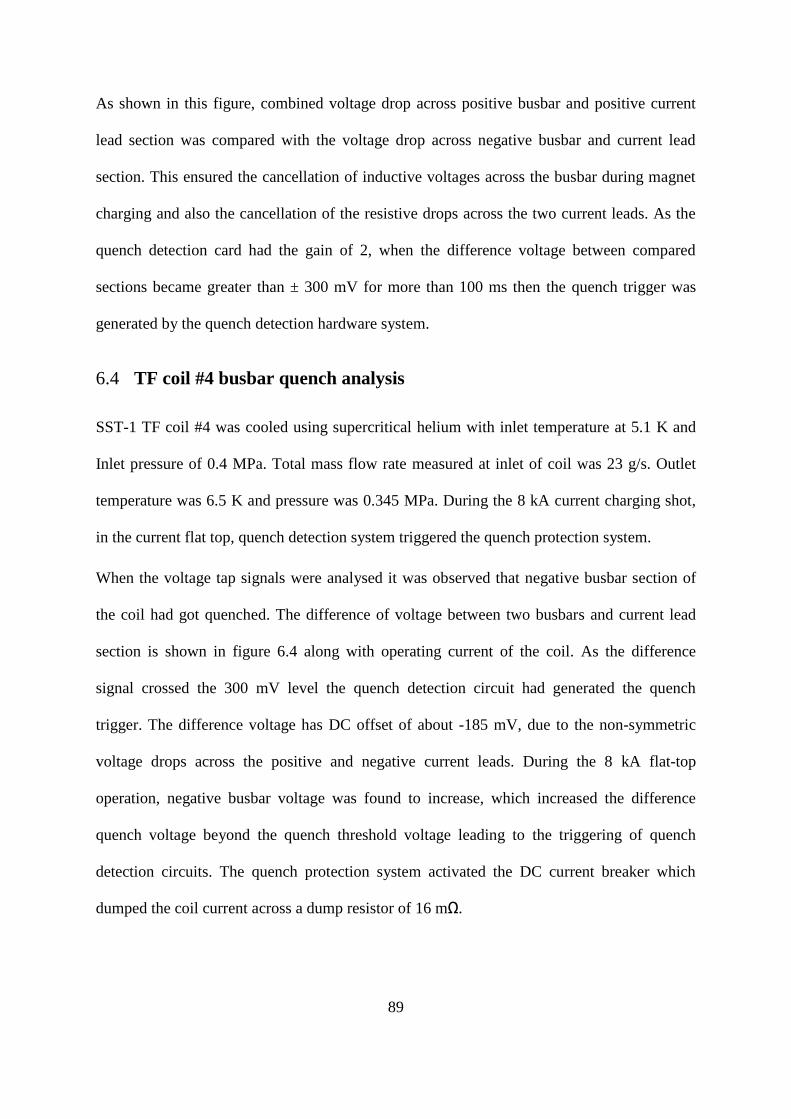
89

As shown in this figure, combined voltage drop across positive busbar and positive current

lead section was compared with the voltage drop across negative busbar and current lead

section. This ensured the cancellation of inductive voltages across the busbar during magnet

charging and also the cancellation of the resistive drops across the two current leads. As the

quench detection card had the gain of 2, when the difference voltage between compared

sections became greater than ± 300 mV for more than 100 ms then the quench trigger was

generated by the quench detection hardware system.

TF coil #4 busbar quench analysis 6.4

SST-1 TF coil #4 was cooled using supercritical helium with inlet temperature at 5.1 K and

Inlet pressure of 0.4 MPa. Total mass flow rate measured at inlet of coil was 23 g/s. Outlet

temperature was 6.5 K and pressure was 0.345 MPa. During the 8 kA current charging shot,

in the current flat top, quench detection system triggered the quench protection system.

When the voltage tap signals were analysed it was observed that negative busbar section of

the coil had got quenched. The difference of voltage between two busbars and current lead

section is shown in figure 6.4 along with operating current of the coil. As the difference

signal crossed the 300 mV level the quench detection circuit had generated the quench

trigger. The difference voltage has DC offset of about -185 mV, due to the non-symmetric

voltage drops across the positive and negative current leads. During the 8 kA flat-top

operation, negative busbar voltage was found to increase, which increased the difference

quench voltage beyond the quench threshold voltage leading to the triggering of quench

detection circuits. The quench protection system activated the DC current breaker which

dumped the coil current across a dump resistor of 16 mΩ.

90

It can be deduced from this voltage development that a normal voltage of 61 mV was

generated in this quench (deduced from observed voltage is 122 mV divided by electronic

card gain of 2) in about 5.3 s. Considering the SST-1 CICC resistance at about 15 K, the total

busbar length of 1.8 m was quenched. This gives an average normal zone propagation speed

in the range of 0.34 – 0.4 m/s. This is found to be quite low as compared to about 5 m/s

observed in TF coil double pancakes. In order to understand the reason of this quench

initiation and its relatively slow normal zone propagation mechanism, it was simulated using

the Gandalf code. This code has been bench marked earlier to simulate SST-1 TF coil in

chapter 5. The input parameters for Gandalf such as mass flow rate, pressure, temperature,

operating current and background magnetic field etc. were taken from experimental details of

TF coil #4 provided earlier. SST-1 CICC specifications, friction factor and heat transfer

correlations, hydraulic model used in the code are similar to that used earlier in chapter 5.

Figure 6.4: Resistive voltage development during TF coil #4 busbar quench

91

Simulation results 6.5

In simulation trials, the quench was generated in the busbar section by applying a square

wave-shaped heat pulse of varying magnitudes and varying lengths as well as on different

locations along the entire length of conductor. The normal zone voltage development was

then compared with the experimental observations of normal zone voltage shown in figure

6.4. After several iterations, it was found that when a heat pulse is applied in a very small

section of 10 mm at the beginning of conductor, the experimental and simulation voltage

profiles match well. This position corresponds to a short support location of the busbar just

after the coil to busbar joint. For comparison of two plots, the DC offset of -185 mV was

added to the simulation voltage. Its time reference also matched with the experimental time.

This comparison is shown in figure 6.5 and its matching is found to be acceptable. The

distinct changes in slopes observed in Gandalf simulation plot coincides with the entire 1.8 m

of busbar being quenched. Since the total voltage across busbar has not reached the quench

threshold voltage level of quench detection card, continuous joule heating increased the

conductor temperature and hence its resistance, till the voltage level across busbar crossed the

threshold voltage limit.

During the experiment, no significant change in temperature was recorded. This is because at

the busbar outlet, helium was fed to the current lead section, which had large supercritical

helium volume. Temperature sensor was installed on outer stainless steel can of supercritical

helium section of current lead. This section is also thermally shorted to LHe section of

current lead which is continuously filled with fresh liquid helium from the plant during

current charging experiments. Similarly mass flow rate and pressure changes experimentally

observed during this quench were found to be small.

92

One reason for observations of lower normal zone propagation speed as compared to those in

the DPs of TF coils is presence of lower background magnetic fields on busbar. Lower

magneto-resistance of copper stabilizer then generates lower joule heating. Another reason is

the absence of transverse quench propagation mechanisms in a single-turn busbar compared

to that in tightly wound double pancakes inside of TF coil. Incidentally, in the Gandalf code

simulation, the transverse conduction of heat is not modelled which contributed to a good

matching of the experimental observations and the simulation results. Good matching of

these results have additionally validated the predictions of SST-1 coil test team that the heat

load coming from short length supports can lead to quench during coil test experiments.

Figure 6.5: The comparison of experimental and simulation normal zone voltage

Recommendation for SST-1 TF magnet feeder quench detection 6.6

It was realized from the experimental observations that the quench propagation speed in

busbar can be very low as compared to the TF coils. Thus, in the case of quench threshold

voltage being similar to that set for the TF coils, it would take longer to reach the threshold

1065 1068 1071

-0.30

-0.25

-0.20

Expt an

d s

imu

lation

no

rmal zone

voltage

(V

)

Time (S)

Experimental data

Gandalf data

Full busbar quench

93

voltage level, which would lead to higher hotspot temperature and probable insulation

degradations. So quench threshold voltage levels must be set to lower values for the busbar.

A threshold voltage level of 52 mV is recommended, which corresponds to 2 m of quenched

length of SST-1 CICC at 0.44 T, for 10 kA operations. Total length of the SST-1 TF magnet

busbar is about 10 m.

Another recommendation was related to the locations of voltage taps. If the voltage taps are

installed as shown in figure 6.3, then current lead DC voltage drop will always be present in

busbar voltage signals. This, in the case of unequal current lead voltage drops, would give

non-zero difference voltage even with no quench in the busbar. Thus separate measurements

of current lead and busbar voltages were recommended and it has been subsequently

implemented in SST-1. This new scheme is shown in figure 6.6.

Figure 6.6: New voltage tap locations for current leads and busbar

During the engineering validation phase of the assembled SST-1 TF magnets, a quench was

observed in the TF busbar section. This quench was triggered by a vacuum failure event in

DP1

PositiveCurrent

Lead

Positive busbar

NegativeCurrent

Lead

Negative busbar

DP6

Voltage taps for quench detection

94

the TF busbar duct, leading to quenching of both positive and negative busbars. The voltage

signals acquired from the new voltage tap scheme of figure 6.6 have given an unambiguous

quench trigger for this event. These voltage signals are shown in figure 6.7. Once the

difference voltage between busbar reached the threshold value, the quench trigger was

generated after the threshold time delay.

Figure 6.7: SST-1: Detection of quench in TF magnet busbar

Thermo-hydraulic simulation of Busbar in assembled TF magnet 6.7

system

SST-1 TF magnet current feeder system’s main components are shown schematically in

figure 6.8. TF magnet busbars terminate in a chamber known as current lead assembly

chamber (CLAC). CLAC and cryostat are connected to each other with stainless steel ducts

95

known as TF duct. The TF duct has liquid nitrogen-cooled thermal shields to reduce the

radiation heat load on to the superconducting busbar. All throughout the length, busbar are

supported on the thermal shield by using several glass fibre supports (G 10 CR) at a spacing

of 600 mm. CICC of the busbar is similar to that used in SST-1 TF and PF magnets. Both

positive and negative TF busbars are about 10 m in length and have two joints each. One joint

is between the Current lead and busbar and the other is between the busbar and the magnet.

Joint with current lead is a bolted lap joint and joint with magnet terminal is a soldered lap

joint. Vacuum barrier with ceramic isolator and stainless steel bellows are installed closer to

magnet side to isolate the cryostat vacuum with CLAC vacuum. Busbars are cooled from

current lead side joint location. The steady-state heat loads acting on the TF magnet system

busbars mainly comprised of conduction from supports and vacuum barriers, radiation,

residual gas conduction (RGC) and joule heating from joints. Actual values of these heat

loads have been calculated. For radiation heat load calculation, the entire busbar is considered

at 4.5 K and thermal shield temperature is considered as 85 K. Emissivity of cold and warm

surface is assumed as 0.2 and 0.3 respectively. Interspace vacuum pressure of 2 x 10-5 mbar

is used for residual gas conduction heat load. For estimating conduction heat load from

supports and vacuum barriers, thermal conductivity integral values between 4.5 K and 85 K

of glass fibre and ceramic and actual geometrical dimensions have been used. Joule heat load

estimations have been done using the joint resistance value of 5 nΩ for the bolted joint

between current lead and busbar and 1 nΩ for the soldered joint between magnet terminals

and busbar. The heat load estimations are summarized in table 6.1.

It is found that the heat loads from supports, vacuum barrier and joints are dominant as

compared to other heat loads. A total heat of 6.46 W is estimated to be acting on each busbar

during 10000 A current operations of TF magnets. In order to compensate for uncertainty in

96

actual contacts from supports etc. and other simplifications or errors in estimations, a safety

factor (SF) of 1.5 is used and the total heat load is taken to 9.7 W for all calculations.

Table 6.1: Steady-state heat load acting of TF busbar

Radiation

(W)

RGC

(W)

Supports

(W)

Vacuum

barrier (W)

Bolted

joint (W)

Soldered

Joint (W)

Total

(W)

Total with SF of

1.5 (W)

0.003 0.025 3.89 2 0.5 0.05 6.468 9.7

Figure 6.8: SST-1 TF current feeder schematic

Thermo-hydraulic analysis of busbar has been done using code HESS [6.1]. It is a code for

steady-state analysis of helium cooled conductors. Heat load from different components as

per table 6.1 were mapped at different locations on the 10 m length of busbar conductor as

per the actual locations of these components in the current feeder system. Under the action of

these heat loads, busbar pressure drop and its outlet temperature were estimated for different

97

mass flow rates under steady-state conditions using HESS. The results are shown in Fig. 6.9.

As seen, the pressure drop is in the acceptable range for the entire flow range of 0.4 g/s to 1.5

g/s. Thus a suitable mass flow rate can be selected purely on the basis of required temperature

margin during SST-1 operation.

The maximum field acting on TF busbar, with all TF and PF magnets fully charged, is

estimated to be about 0.44 T near the tokamak side. At other locations, busbar will be in the

self-field of 0.22 T. Near the current lead side, where busbar bends at an angle of 135

degrees, self-field is enhanced to 0.28 T. Considering the worst case scenario, the entire

busbar is considered in a background magnetic field of 0.44 T. At this magnetic field and

10000 A operating current, current sharing temperature of SST-1 CICC is calculated to be

about 7.7 K [6.2]. As seen in figure 6.9, outlet temperature is 5.83 K at the mass flow rate of

1 g/s which gives a temperature margin of 1.9 K. This is acceptable and so this mass flow rate

is recommended for TF busbar. Two dedicated Venturi mass flow meters have been installed

on these paths to monitor the flow and provide necessary feedback to the helium plant for

controlling the flow rate close to 1 g/s.

Figure 6.9: Pressure drop and outlet temperature for different mass flow rates

98

Conclusion 6.8

Quench observed in busbar during the single coil tests of SST-1 TF magnet has been

analyzed in detail and quench propagation speed has been estimated. A propagation speed in

the range of 0.34 – 0.4 m/s has been observed. This speed is quite low when compared to

those observed during TF coil quenches involving DPs. These fundamentally different

characteristics are primarily attributed to a lower acting background field on busbar and

absence of transverse thermal conduction like in double pancake windings. Such slow quench

propagation has been successfully simulated with the Gandalf code. A steady-state thermal

load of about 10 W has been calculated to be acting on actual SST-1 TF magnet busbars. A

mass flow rate of 1 g/s will be sufficient to compensate this heat load and will give a

temperature margin of 1.9 K, which ensures a safe and cryo-stable operation of SST-1 TF

magnets. These analyses results have been reported in [6.3].

99

7. CICC Design study

Design of CICC for fusion magnet application involves optimization of several parameters

like strand design, conductor sizing, void fraction, jacket material and jacket thickness [7.1 -

7.3]. These parameters in turn depend on operating magnetic field and current requirements,

plasma operation scenarios and magnet current ramp rate requirements, etc. The objective is

to get an optimized design of a CICC such that the magnet should not quench during any

planned tokamak operational scenarios. And if quench occurs, CICC should be able to bear

the effects of quench. While CICC design is a very vast topic for the scope of this work,

optimization of stabilizer area in strands of CICC is discussed in this chapter. It has a direct

impact on the stability and the quench characteristics of CICC [7.4]. Generally, a high RRR

copper and aluminium are the preferred choice for stabilizer. A NbTi/Cu based, high current

and high field virtual conductor is used for this case study using Gandalf.

Copper to Superconductor ratio in Strands of CICC 7.1

7.1.1 The virtual conductor

A virtual conductor was considered for this case study. Its operating current is 26.5 kA and

operating peak magnetic field is 6.5 T. The CICC cross-sectional area, void fraction (helium

area), inlet temperature mass flow rate and jacket thickness are fixed for this CICC. The aim

is to find the suitable copper to superconductor NbTi ratio (Cu: SC) in the area allotted for

strands in the CICC. This ratio decides the quench behaviour (from copper stabilizer area)

and the stability margin (discussed later) of the CICC. Gandalf code is used as a tool to study

this critical optimization.

100

It is a square conductor of side 29.1 mm (including 3.5mm thick SS304L jacket) with

following allocated space for different components and major operating conditions:

Helium section = 161.3 mm2

Composite section (NbTi + Copper): 287 mm2

Strand diameter: 0.712 mm

Inlet pressure = 0.6 MPa

Mass flow rate = 1 g/s

Inlet temperature = 4.6 K

Insulation thickness = 2 mm

7.1.2 Stability

Superconducting magnets experience a wide spectrum of disturbance (external energy

deposition) during tokamak operations. Mechanical energy release by wire movement,

insulation de-bonding or epoxy cracking, AC losses and plasma disruptions are some

examples of disturbances of different magnitude, timescale and spatial distribution [3.2]. The

maximum energy which could be absorbed by strands without getting quenched is known as

stability margin ‘Ec’. In this study using Gandalf, heat will be deposited on different

conductor lengths and for different time scales. Stability margin will be calculated from the

maximum heat energy absorbed by CICC without getting quenched, using equation 7.1. It is

generally expressed in mJ/cc of the composite. The disturbances selected for stability study

should represent the typical disturbance expected on the magnets.

𝐸𝑐 =𝑄

𝐴𝑐𝑢+𝐴𝑆𝐶 × 𝛥𝑡 (7.1)

where Q = total heat deposited in Watt

101

ACu = Copper Cross section in NbTi strands (m2)

ASC = Superconductor cross section (m2)

Δt = time duration of disturbance of square shape (s)

7.1.3 Classical model of stability

Insufficient stability margin and large disturbances were the main reasons of failure of earlier

magnets. In 1965 Stekly and Zar gave the concept of cryostability [7.5]. Cryostability was

achieved when the composite temperature with the full operating current flowing in the

stabilizer was below the critical temperature of the superconductor. It was represented in

terms of Stekly criterion α < 1 and

𝛼 = 𝜌𝐼2

ℎ𝑃𝑤𝐴(𝑇𝑐−𝑇𝑜𝑝)< 1 (7.2)

Where

h = steady-state heat transfer coefficient, Pw = wetted parameter of conductor, A = Stabilizer

cross-section, I = current in the conductor, ρ = matrix resistivity, Tc = critical temperature, Top

= operating temperature

This concept of cryostability is not applicable for CICC as the helium available as heat sink is

not infinite, rather it is limited and its temperature increases during the disturbance.

Application of this criteria leads to requirement of very high copper area in the CICC strands.

Numerical code Gandalf is more suitable for estimating the stability of CICC as exact helium

volume is used in calculation and it treats the temperatures of helium, strands and jacket

separately and the energy balances are coupled via heat transfer coefficients at the contact

(wetted) surfaces. CICC are designed as metastable with ability to operate at specified

102

nominal current density with an ability to withstand the specified spectrum of external

disturbances.

7.1.4 Copper to superconductor ratio

The subject of ratio of copper stabilizer and superconductor in CICC strands, known as Cu:

SC ratio is an important design parameter of CICC. It has a direct impact on the stability and

the quench protection characteristics of the CICC. As discussed in chapter 3 of this thesis, if

external disturbance raises the strand temperature above current sharing temperature Tcs, joule

heat generation is initiated. The available temperature margin for operation is the difference

between the operating temperature and Tcs. Also, as described in equation 3.3, Tcs depends

directly on the section of superconductor in the strand, so available temperature margin

depends on the section of superconductor.

It is known that copper in the conductor plays an important role in reducing the maximum

hotspot temperature. If copper area is more, a higher discharge time dis can be allowed for

the similar maximum hotspot temperature. Higher discharge time helps in reducing the dump

voltage as lower value dump resistor could be selected.

In the study of the virtual conductor with a fixed conductor cross-section and a fixed load line

we will study the effect of variation of copper and superconductor ratio using Gandalf.

Different cases studied using Gandalf 7.2

In this section, a virtual conductor is studied with the total NbTi and copper composite

section fixed to 287 mm2. Stability and protection aspects were studied for four Cu:SC ratios

to cover the wide range from less than 1 to about 7. The specific ratios studied are given in

table 7.1.

103

Table 7.1: Different Cu: SC ratio used for stability studies

Sr. No. SCu (mm2) SNbTi (mm

2) Cu:SC ratio

1 252.1 34.6 7.28

2 239.2 47.5 5.03

3 212.2 74.5 2.84

4 127 160 0.79

The time step and mesh size were finalized after detailed convergence studies. Table 7.2

gives the exact details of different parameters used in Gandalf.

Table 7.2: time and mesh sizes used in Gandalf

Parameter 100 ms on 1m 10 ms on 1 m 1 ms on 0.01 m

Total conductor length in simulation 4 m 4 m 1.2 m

Time step 0.1 ms 0.01 ms 0.001 ms

Mesh size (length) 1 mm 1 mm 0.03 mm

Results of the stability study 7.3

Three disturbances of 100 ms on 1 m, 10 ms on 1 m and 1 ms on 10 mm were selected for

stability study as these represent the typical disturbances related to plasma disruption, AC

losses and wire movements in tokamak magnets. The total conductor lengths for simulation

were chosen to be sufficiently longer to avoid the cable end effects. SST-1 CICC Jc-B

relationship was implemented in Gandalf. The magnetic field was uniform over the conductor

length. The input data for the Gandalf code was generated from the details of the virtual

conductor provided earlier. Different amount of heat energy were put on the heated lengths of

the conductor and iteratively the maximum allowable heat deposition was calculated for all

104

the three cases seen earlier. The available temperature margins for these cases were also

found out from the code. These results for three cases are given in table 7.3 to 7.5.

Table 7.3: Results of 100ms disturbance on 1 m length

T Margin (K) ANbTi (mm2) ACu (mm

2) Cu:SC Stekly

Parameter

Stability margin

(mJ/cm3)

0.8 34.6 252.1 7.28 0.59 166

1 47.5 239.2 5.03 0.62 209

1.2 74.5 212.2 2.84 0.70 237

1.4 160 127 0.79 1.18 261

Table 7.4: Results of 10 ms disturbance on 1 m length

T Margin (K) ANbTi (mm2) ACu (mm

2) Cu:SC Stekly

Parameter

Stability margin

(mJ/cm3)

0.8 34.6 252.1 7.28 0.59 211

1 47.5 239.2 5.03 0.62 238

1.2 74.5 212.2 2.84 0.70 249

1.4 160 127 0.79 1.18 91

105

Table 7.5: Results of 1 ms disturbance on 0.01 m length

T Margin (K) ANbTi (mm2) ACu (mm

2) Cu:SC Stekly

Parameter

Stability margin

(mJ/cm3)

0.8 34.6 252.1 7.28 0.59 1414

1 47.5 239.2 5.03 0.62 1625

1.2 74.5 212.2 2.84 0.70 1606

1.4 160 127 0.79 1.18 750

As seen from these tables, Cu: SC ratio of 2.84 corresponding to temperature margins of 1.2

K is the most suitable to get high stability margin for all disturbance scenarios. This option

was then further investigated for the protection studies.

Also, it is observed that the critical energy in some cases decreases when the Stekly

parameter decreases which is contrary to the Stekly criterion. A larger critical energy was

found associated with the higher Stekly parameter. This is because the helium volume

available to remove joule heating in CICC is not infinite, as assumed in this criterion.

Additionally, for disturbances on small lengths like 0.01 m, heat conduction can also play a

role which is not considered in the Stekly criterion. This justifies the use of numerical codes

like Gandalf rather than the classical analytical tools for designing CICCs with a specified

minimum stability margin and for a spectrum of expected disturbance.

106

Results of protection studies 7.4

Figure 7.1: Copper section needed for protection as a function of τdelay and τdump

The copper section (Scu) is a direct function of allowable dump time constant to limit the

hotspot temperature below the prescribed limit. For the virtual conductor, with Cu:SC ratio of

2.84, we can find by the classical approach of total adiabaticity, the dump time constant

limiting the hotspot temperature to 250 K. Two cases of 1 s and 2 s hold time are considered

to see if the copper area is sufficient. The result is shown in figure 7.1. As observed, dump

time constant of maximum 15 s is allowed for the case of 2 s hold time (τdelay) to limit the

hotspot temperature to less than 250 K.

Conclusion 7.5

The virtual conductor example was used to show the possibility of use of Gandalf code to

design CICC for a specific stability margin. The conductor version with the temperature

margin of 1.2 K is preferable for higher stability margin. The total copper section is such that

107

a time constant as large as 15 s can be considered for the safety discharge associated with a

detection delay of 2 s.

108

8. Quench detection of SST-1 TF coils by helium flow and

pressure measurement

TF magnets of SST-1 are cooled by supercritical helium at 4.5 K and 0.4 MPa. Two types of

Venturi meters (VM) are used for measuring helium mass flow rates in these magnets. Signal

conditioning for temperature, absolute pressure and differential pressure sensors and a

suitable data acquisition system have also been developed for these flow meters. These flow

meters were extensively qualified during single-coil test campaigns of SST-1 TF coils. Mass

flow and pressure signals behaviour during quench events of TF coil tests were analysed and

a quench detection system using these signals has been proposed for TF coils. This secondary

quench detection methodology and its hardware development are discussed in this chapter.

VM design, fabrication, installation and the flow measurement system are also described in

this chapter.

Cryogenic flow distribution system 8.1

SST-1 TF magnets will be cooled by SST-1 cryogenic plant comprising a 1.3 kW at 4.5 K

Helium Refrigerator/Liquefier (HRL) system, which is the largest He cryogenic plant in

India. The operation features of HRL include controlled cooling down and warming up of the

magnet system from 300 K to 4.5 K and vice versa, operation in double-phase mode and

supercritical mode, absorption of transients from SST-1 during ramp-up/down of the

magnets, plasma operations and handling abnormal events like magnet quench. The cold

circulator provides 300 g/s supercritical helium at 4.5K, 0.4 MPa. The Integrated flow

distribution and control (IFDC) system, divides this flow in three major hydraulic paths: the

TF system, the PF coils and the case cum support structure. A separate path for TF and PF

109

busbar also exists. Its schematic is shown in figure 8.1. An accurate measurement of helium

flow is required over a wide range of operating parameters to ensure efficient operation and

control of cryogenic plants and to characterize the superconducting magnets [8.1]. Flow

measurement of individual sections is done with venturi mass flow meters.

Figure 8.1: Block diagram of IFDC system and its interface with SST-1

Design of Venturi meters 8.2

VM was selected for flow measurement because of its inherently low pressure drop, easy

fabrication, high repeatability of measurement and no wear and tear over long-term operation.

The supercritical helium mass flow rate design values for individual superconducting magnet

of SST-1 Magnet system are given in table 8.1.

110

Table 8.1: Supercritical helium mass flow rates of SST-1 Magnets

Coil Number of flow

paths, average path

lengths

Design mass flow

rate in each flow path

(g/s)

Total mass flow rate

in one coil (g/s)

TF

(16 coils)

12 paths, 48 m 1.25 15

PF1

(1 coil)

2 paths, 113 m 0.9 1.8

PF2

(2 coils)

1 path, 113 m 0.9 0.9

PF3

(2 coils)

8 paths, 75 m 1.1 8.8

PF4

(2 coils)

4 paths, 113 m 0.9 3.6

PF5

(2 coils)

4 paths, 130 m 0.8 3.2

VMs are generally designed and manufactured according to the standards ISO-5167. These

flow meters rely on the differential pressure measurement through the constricted section and

the density estimation at the inlet of the VM with dedicated pressure and temperature

measurements. When designing a VM for LHe service, its main dimensions can be derived

by scaling down those which are advised by the ISO -5167 standard [8.2].

111

Figure 8.2: typical inner profile of VM

The VM inner profile can be divided into four main parts shown in figure 8.2:

upstream section: cylindrical, with diameter D equal to that of the upstream pipe and

length at least equal to D

throat section: cylindrical, with diameter and length equal to d

converging section: conical, connecting the upstream and the throat sections with

semi-angle aperture ‘α’ of (10.5 ± 0.5)°

diverging section: conical, with initial diameter d and final diameter D, here the semi-

angle aperture δ is (4 ± 0.5) °

Using these guidelines two VMs were designed to meet the wide range of SST-1 flow

measurement requirements. One is for TF coil and the other for PF coil flow measurement.

αδ

throat

sectionAnnular chambers

D D

for differential pressure

measurement

upstream

section

112

The VMs were designed to give an easily measurable range of differential pressure across its

upstream and downstream section [8.3]. The details of both types of VM are given in table

8.2. VMs were fabricated by precision machining of SS304L metal bars. The tapered

structures were made by wire cut with a 2-delta finish. After fabrication of these, the

dimensions were measured by using custom made dies. Six radial holes were made in the

upstream and throat section each. These holes connected to annular chambers with tubing

welded for differential pressure measurements as shown in figure 8.2. After final fabrication

VMs were ultrasonically cleaned, electro-polished and helium leak-tested with an acceptable

leak rate of ≤ 1 x10-8

mbar l/s.

Table 8.2: Details of venturi meter construction

Type Throat

diameter,

length (mm)

Upstream,

Downstream

diameter (mm)

Downstream

semi-angle

(degrees)

Upstream

semi-angle

(degrees)

Total length

(mm)

TF 6 12 10.5 4 120

PF 4 8 10.5 4 90

Calibration of venturi meter 8.3

Mass flow rate through a VM is given by

𝐺 = 𝐶𝑑𝐴𝑡√2𝜌𝑃𝑑

1−𝛽4 (8.1)

Where:

G = mass flow rate [kg/s]

At = throat section area [m2]

113

Pd = pressure difference across upstream and throat [Pa]

Cd = discharge coefficient

ρ = fluid density [kg/m3]

β = throat to upstream diameter ratio

As per equation (8.1), all quantities required for estimating flow rate can be directly measured

except Cd which needs to be obtained experimentally by calibration. Both TF and PF VM

were calibrated using a standard mass flow meter connected in series with the VM. Using the

mass flow rate values from standard mass flow meter and the measured ΔP across the VM, Cd

has been estimated for both these flow meters over a range of mass flow rates applicable for

SST-1. The discharge coefficient of VM tube with a machined convergent entrance varies

slightly with the Reynolds number [8.4]. Since in our case the highest accuracy was desired

at low-temperature conditions, constant discharge coefficient equal to 1 was considered for

both these VMs. This simplification introduced an inaccuracy of about 3% in the flow

measurement. The total accuracy of flow measurement can be calculated by simplified root

mean square method after considering additional inaccuracies of differential pressure,

absolute pressure and temperature measurement [8.5]. For TF and PF VMs it is estimated to

be about 3.18 %.

Venturi meter installation on SST-1 Magnets 8.4

Twenty seven VMs are installed on SST-1 magnets namely on the outlet side of each TF

magnet, inlet of all 9 PF coils and on 2 CICC busbar inlets of TF magnets. Locations of VM

installation were made on the basis of available space inside the SST-1 machine shell. Figure

8.3 shows the schematic of VM installed on TF magnet outlet side. VMs were installed in the

system by welding the units into the process piping. In order to ensure that the velocity of the

114

fluid at the VM is primarily axial and swirl free, a straight pipe of 350 mm was kept at the

upstream of the VM [8.6]. Stainless steel tubings of 6 mm O.D. and 1 mm thickness were

welded into the pressure tap sockets of the VM (not shown). These tubing were extended

outside the cryostat through vacuum flanges. The possible heat load from these tubing onto

the magnet was estimated to be 6 mW per tube and 12 mW per VM. This was calculated

using the integrated thermal conductivity of SS from 4.5 K to 300 K. Each tubing length was

minimum 6 m inside the cryostat and was anchored to liquid nitrogen header to reduce the

heat load onto the magnets. As VMs were welded after the electrical break the possibility of

electrical shootings due to long SS tubing could be avoided.

Figure 8.3: TF coil VM installed on the outlet manifold of TF coil

VM

115

Figure 8.4: Differential pressure tubing of VM welded onto vacuum flange of cryostat (top

left), valve fittings before the pressure transducers, current to voltage convertors with

isolation for connection of transducer output to VME (top right)

The temperature measurements were available from the temperature sensors already installed

on individual coil outlets. Absolute pressure was measured by a Keller PR-21Y transducer

and differential pressure was measured using a Siemens 7MF4433 transducer. There was

concern about the possibility of helium leak in tubing connections from VM up to these

transducers. To take care of this issue, all the connections inside the cryostat from VM to

vacuum flanges were welded connections. Outside the cryostat, Swagelok make SS below

sealed valves were installed between the cryostat vacuum flange and the transducers. Tubings

116

with high quality surface finish were used to avoid leaks from the Swagelok connectors. In

the case of leak or transducer malfunction, online repair could be done by isolating the

transducers from the process line by using valves, whenever required.

VME-based data acquisition system was used to acquire signal from all the transducers [8.7].

The 4-20 mA output of pressure transducers was electrically isolated and converted to 1–5 V

before connection to the VME. Mass flow rate was calculated using the relevant sensor data

and helium property database for density estimations.

These flow meters have been extensively used to measure the helium mass flow rates at

operating conditions, during several SST-1 campaigns, single TF coil test experiments and

lab scale experiments [4.4][8.8]. Several component of these flow meters installation set-ups

are shown in figure 8.4. Mass flow rate measured using different VMs at different

temperatures during the SST-1 cool down is shown in figure 8.5.

Fig. 8.5 Mass flow rate during cool down of SST-1 magnets

0

0.5

1

1.5

2

2.5

3

3.5

4

0 50 100 150 200 250 300

Mas

s fl

ow

rat

e (g

/s)

Temperature (K)

TF1

TF2

TF3

TF4

PF1

PF2B

PF3B

PF4B

PF5B

117

Quench detection methods 8.5

Superconducting magnets operating in high magnetic field, with high current density and

limited operational stability margins, like that of tokamaks or stellarators, always have finite

probability of getting quenched during operations. Quench is an off normal event, wherein a

resistive zone (also called normal zone) develops along a superconducting conductor. The

joule heating of the initial resistive zone heats the additional conductor lengths, as well as the

coolant being the vector of further propagation of normal zone. If protection actions are not

taken in time, extensive damages like conductor melting, arcing, coolant pressure increase

and expulsion etc. can occur and damage the magnet system beyond repairs. Therefore

quench must be detected at the earliest possible to insert external resistors in the circuit and

dump the magnetic energy into this resistor and protect the magnet from thermal damage. So

reliable quench detection and protection aspects must be incorporated in the design of every

superconducting magnet system.

Voltage measurement is one of the fastest and widely used methods of quench detection

[3.4]. In this method, voltages across different identical sections of magnets are compared.

When a section of magnet is quenched, it develops additional voltage and when it crosses a

certain threshold voltage level and stays above this level for a certain threshold time, a

quench trigger is generated by quench detection hardware and magnet energy extraction

process is initiated. This method has also been successfully implemented for SST-1 TF coils

[4.5, 4.6].

Quench can also be detected by monitoring non-electrical signals from like mass flow rate

and pressure [8.9 - 8.11]. Any significant change in the steady-state operational values of

these signals can indicate a fault condition like quench inside the magnet. These are

inherently slow signals and are expected to give slow response to the quench process, but can

118

be used as a secondary quench detector. This redundancy could be very useful in case of

major malfunction or failure of the primary quench detector. Following this philosophy, a

hydraulic signal-based secondary quench detection system has been proposed for SST-1 TF

magnet.

Hydraulic quench detection 8.6

A quench detection method has been proposed based on monitoring the changes in nominal

flow and pressure values rather than crossing above or below a certain value and based on the

venturi meters described in the preceding section. This has been done to accommodate for

measurement uncertainty in mass flow and pressure signals and to avoid requirement of flow

path dependent threshold settings. Also drawing analogy from voltage measurement-based

quench detection methods, thresholds for time and levels are proposed after review of coil

test data.

Figure 8.6: mass flow change during TF5 coil quench

608 612 616

0

50

100

2nd flow trigger

delayed by 6 sec

TF5 Quench

1st flow trigger

delayed by 1.2 sec

Pe

rce

nta

ge

ch

an

ge

in

flo

w

time (s)

Inlet

Outlet

Quench Trigger

by Voltage Signal

119

It is proposed that if mass flow/pressure data register more than 50 % change in its nominal

value (similar to threshold voltage) and if this change continues for more than 500 ms

(threshold time) quench trigger will be generated.

The TF5 flow data trends during quench are shown in figure 8.6. The difference between the

time taken for reaching flow/pressure thresholds and for reaching the voltage-based quench

detection threshold are shown as delay. As seen for TF5, the mass flow change at outlet

crossed the threshold with a delay of 1.2 s and at inlet with a delay of 6 s. For TF2 coil as

seen from figure 8.7, the mass flow change at outlet crossed the threshold without any delay

and at inlet with a delay of 5 s. The study of signal from other coils revealed that always at

least one of the inlet or outlet mass flow rate always crossed the threshold with delay less

than 2 s.

Fig. 8.7 mass flow change during TF5 coil quench

640 660 680

0

100

200

Second flow Trigger

has 5 second delay

First flow Trigger

has no delay

Pe

rce

nta

ge

ch

an

ge

in

flo

w

time (s)

Inlet

Outlet

Quench Trigger by

Voltage signal

TF2 Quench

120

Figure 8.8: Pressure changes during TF11 and TF3 coil quench

Similarly the pressure data trend for all quench cases has been studied. Fig. 8.8 shows the

pressure trends for coil TF11 and TF3 at coil inlet and outlet with delay times with respect to

voltage based quench detection. As observed, the minimum delay time for reaching the

121

pressure threshold is 1.3 s. The study of pressure signals from other coils revealed that always

at least one of the inlet or outlet mass flow rate always crossed the threshold with a delay of

less than 2 s.

These observations of flow and pressure signals have confirmed that use of hydraulic-based

quench detection system for SST-1 TF magnet system is feasible. As in SST-1 tokamak the

quench-induced flow and pressure changes will be higher than in single coil test, due to

higher joule heating. The peak magnetic field on TF conductor is 5.1 T as compared to peak

field of 2.2 T in coil test environment, giving rise to higher magneto-resistance of copper

stabilizer resulting in higher joule heating.

Thermo-hydraulic simulation of TF magnet is SST-1 tokamak assembly was done to simulate

the possible effects of failure of voltage-based quench detection system and quench detection

by hydraulic means with a delay of 3 s. This time was conservatively chosen higher than the

maximum delay of either flow or pressure-based first triggers observed in TF coil test

campaigns. Gandalf was used for these simulations. The input parameters for Gandalf such as

mass flow rate, pressure, temperature, operating current and background magnetic field etc.,

were obtained from SST-1 TF magnet system nominal operating values. SST-1 CICC

specifications, friction factor and heat transfer correlations and the hydraulic model used in

the code are similar to that used earlier in chapters. This simulation was done to estimate the

maximum hotspot temperature and maximum pressure rise observed if quench detection is

delayed by 3 s. The results are shown in figure 8.9 and 8.10. As seen the peak temperature

reached within the conductor length is about 178 K and the peak pressure is 9.5 bar. This is

still within the safe limits of SST-1 CICC design.

122

Figure 8.9: Temperature rise from Gandalf simulation in case of delayed quench detection

Figure 8.10: Pressure rise at the hotspot from Gandalf simulation

0 10 20 30 40

0

20

40

60

80

100

120

140

160

180

Te

mp

era

ture

(K

)

X length (m)

temperature profile

0 5 10 15 20 25 30

4

5

6

7

8

9

10

Pre

ss

ure

(b

ar)

time (s)

Pressure rise at the centre

of Hot spot

123

Proposal for quench detection hardware 8.7

A quench detection hardware schematic is also proposed for flow-based secondary quench

detection system. It is shown in figure 8.11. As shown the voltage value corresponding to the

actual flow during operation in TF1 coil to TF16 coils is taken from corresponding

differential pressure transmitters (DPT) of venturi flow meter installed at outlet. These are

compared with the voltage reference value corresponding to the nominal operating flow of 16

g/s. The window comparator continuously compares these two voltages. In normal

operational scenarios of no quench, the difference between DPT and the voltage reference

will be zero or some small values due to possible flow variation between coils from the

nominal 15 g/s.

The window comparator output will become high (+5 V) from low (0 V) if the difference

becomes higher than the voltage corresponding to 24 g/s or lower than the voltage

corresponding to 8 g/s. This high signal will be transmitted to OR circuit only if it remains

high for more than the delay time of 500 ms. After this, the ORing circuit will generate a

quench trigger. Similar circuits can also be implemented for pressure-based quench detection.

Figure 8.11: Schematic of flow based quench detection hardware

124

Conclusion 8.8

Venturi meter-based flow measurement system has been designed and developed for SST-1

magnet system. This system has been successfully used for helium flow measurement during

the TF coil test experiments and on the assembled TF magnet system during engineering

commissioning and plasma experiment phase of SST-1. A secondary quench detection

system based on flow and pressure measurement has been conceptualized for the SST-1 TF

magnet system. The flow and pressure trends during quenches observed in single coil test

experiments have been used to quantify the quench detection system logic. A schematic is

also proposed for development of suitable hardware for this secondary quench detection

system. Work is reported in [8.12].

125

9. Summary and future scope of work

Summary 9.1

Analytical model of SST-1 CICC for estimation of hotspot temperature was developed

assuming complete adiabatic conditions during quench development. This model was used to

design the quench protection system of the SST-1 TF magnet system. The dump resistor was

selected to limit the temperature to less than 115 K and voltage to less than 1 kV. This

method is found to be very useful for quick first order estimation of maximum temperature in

CICC after quench initiation and current dumping.

A simple direct difference algorithm was selected to cancel inductively-coupled voltages on

the coils for accurate quench voltage measurement on TF coils. State-of-the-art, fail safe

quench detection cards were developed using this algorithm. Its main features are precise and

tuneable voltage and time thresholds, and inbuilt complete redundancy. These cards were

successfully tested in several TF coil test campaigns and during the TF magnet system

engineering validations and SST-1 plasma experiments. No failure leading to undetected

quench has been observed with these cards. The card architecture was kept flexible to allow

its use for quench detection of busbar and current leads. These cards will also be also used for

PF magnet quench detection.

SST-1 Toroidal Field coils were individually cold-tested in a dedicated campaign spanning

from June 10, 2010 till January 24, 2011. The electromagnetic, thermal hydraulic and

mechanical performances of each TF magnet was qualified at its nominal operating current of

10000 A in either two-phase or supercritical helium cooling conditions. During the current

charging experiments, few quenches were observed in some of the TF magnets.

126

A commercially available 1-D Gandalf code is a popular code to study the quench

characteristics of CICC-based magnets. This code was adapted to correctly represent SST-1

CICC. Friction factor is an important input parameter in simulation of quench of CICCs. It is

different for each CICC. An experiment was done using pressurized water to determine SST-

1 CICC friction factor as a function of pressure drop. Holman correlation was used to model

the steady-state heat transfer coefficient. This correlation which has direct dependence on

friction factor was adapted in the code subroutine. Critical current density as a function of

magnetic field was also implemented in the code so as to accurately reproduce experimental

results from the SST-1 CICC test.

A variety of possible hydraulic models were studied. Results of these different models were

studied and a suitable model was proposed and implemented in the code to generate accurate

flow conditions as observed during coil test.

Magnetic field on individual DPs was calculated using MAC code. The spatial variation of

magnetic field was implemented in the subroutine of Gandalf for use in quench simulation.

Detailed convergence study was done to gain the confidence in the numerical solutions of

quench studies, which is a complex and highly non-linear problem. The minimum required

time and space discretization steps were determined such that the results were then not

changed by the further refinement of these parameters. Suitable time steps and mesh sizes

were then used in the quench simulation.

The quench observed in TF coil #15 at 8960 A current was simulated using this code and the

developed subroutines. The simulated temperature rise and the quench propagation were

found to be in good agreement with the experimental data.

127

Observation of flow increase at inlet, following quench, was reported from the TF coil test

experimental observation. This was investigated and found to be linked with the dynamic

behaviour of the cryogenic plant.

The CICC model and subroutines developed for TF coil #15 were also used for predictive

quench simulation of the SST-1 TF magnet system.

During the coil test campaigns, TF magnets were connected to a pair of conventional

vapour-cooled current leads through a pair of CICC busbars of about 1.8 m length inside the

test cryostat. Quench observed in the busbar section was experimentally found to have a very

low propagation velocity of 0.34 – 0.4 m/s, as compared to about 5 m/s observed in double

pancake windings of TF magnets. This slow propagating quench was analysed and simulated

successfully using Gandalf. These fundamentally different quench propagation characteristics

were attributed to the lower background magnetic field on the busbar and the absence of

transverse thermal conduction in the busbar which exists in double pancake windings.

Recommendation for low threshold voltage of 52 mV was made for busbar quench detection.

The rearrangement of voltage taps was also proposed for busbar quench detection.

Heat loads were estimated for TF magnet system busbar in the SST-1 tokamak. Steady-state

thermo-hydraulic analyses of the busbars were carried out to find the optimum helium mass

flow rate and for the required operational temperature margin of more than 1.5 K during SST-

1 tokamak operations. A mass flow rate of 1 g/s is found to be sufficient to compensate the

estimated heat load and to give a temperature margin of 1.9 K, which ensured safe and cryo-

stable operation of the SST-1 TF magnets.

The virtual conductor example was used to show the possibility of use of Gandalf code to

design CICC. The stability of this conductor was studied for the disturbance of 100 ms on 1

m, 10 ms on 1 m and 1 ms on 10 mm as these represent the typical disturbance related to

128

plasma disruption, AC losses and wire movements in tokamak magnets. The conductor

version with the Cu: SC ratio of 2.84 was found to be preferable with higher stability margin

for all three disturbances. Using the classical adiabatic approach of hotspot temperature it was

found that for this Cu: SC ratio, maximum dump time constant of 15 s is allowed with a

detection delay of 2s.

Venturi meter-based flow measurement system was designed and developed for SST-1

magnet system. This system was successfully used for helium flow measurement during the

TF coil test experiments and on the assembled TF magnet system during engineering

commissioning and plasma experiment phase of SST-1. A secondary quench detection

system based on flow and pressure measurement was conceptualized for SST-1 TF magnet

system. The flow and pressure trends during quenches observed in single-coil test

experiments were used to quantify thresholds limits for this secondary quench detector

system. A schematic was also proposed for development of suitable hardware for this

secondary quench detection system.

These works have led to successful development of quench detection and protection system

of the first superconducting tokamak of India, SST-1. The quench simulation results were

found to be in good agreement with the experimental observations.

Future Scope of work 9.2

The quench detection circuits developed as a part of this work, could be utilized to develop

advanced noise-cancellation schemes to cancel out inductively-coupled voltages. For

example, the voltages after the isolation and filter stages of the quench detection card could

be acquired in fast DAQ system and noise cancellation schemes could be implemented in

129

software program. This will make this system more versatile, allowing flexibility in

cancellation logics, channels to be compared and in selection of the threshold limits.

These quench detection circuits can also be used to test the use of co-wound tapes for quench

detection of future magnets of IPR.

The quench simulation models developed could be extended and modified to study quench

behaviour of the proposed Nb3Sn based central solenoid of SST-1 tokamak. This will be

useful, as the future fusion reactor magnets in India are expected to be made with Nb3Sn

conductors.

With the generation of additional experimental data from the hydraulic-based quench

detectors, its suitability for use with fast current changing magnets like PF coils and central

solenoid could be verified. This technique, along with voltage-based quench detection

technique, can ensure more reliable quench detection of these magnets.

130

10. References

[1.1] www.iter.org

[1.2] D. Maisonnier, “DEMO and fusion power plant conceptual studies in Europe”, Fusion

Engineering and Design Volume 81, Issues 8–14, February 2006, Pages 1123–1130

[1.3] Weston Stacey, “Fusion”, WILEY VCH, Verlag GmbH & Co. KGaA, Weinheim, 2010

[1.4] WESSON J., "Tokamaks", Oxford University Press, USA; 4 edition (August 1, 2011)

[1.5] P.N. Haubenreich et al., “Superconducting magnets for fusion”, Nuclear fusion, Vol 22,

No. 9, (1982), 1209-1236

[1.6] SERIO L., “Challenges for cryogenics at ITER”, Advance in Cryogenic Engineering,

45, 2010, page 651

[1.7] B. Seeber, “Handbook of Applied Superconductivity”, IOP publishing limited, Bristol

and Philadelphia, 1998

[2.1] S. Pradhan et al. “Status of SST-1 refurbishment”, J. Fusion Res. Series, vol. 9, pp. 650–

657, 2010

[2.2] S. Pradhan et al. “Superconducting Magnets of SST-1 Tokamak”, 20th

IAEA Fusion

Energy Conference (2004), FT3-4Rb

[2.3] S. Pradhan et al. “Superconducting cable-in-conduit-conductor for SST-1 magnets”, in

Proc. 2nd IAEA TCM on Steady-state Operation of fusion devices, Fukuoka, Japan, 1999,

vol. II, p. 482.

[2.4] S. Pradhan et al. “SST-1 poloidal field magnets”, in Proc. 17th IEEE/ NPSS Symposium

on Fusion Eng., San Diego, CA, USA, 1997, pp. 665–668.

131

[2.5] V. L. Tanna et al. “Recent progress and development of cryogenics system towards

Refurbishment of SST-1”, Indian J. Cryogenics, vol. 38, no. 1–4, pp. 87–92, Jan. 2013.

[2.6] Sarkar B et al. “1 KW class Helium Refrigerator/Liquefier system for SST-1”, ICEC-

18, Narosa Publication, New Delhi, pp. 123-126, 2000

[2.7] Z. Khan et al. “Vacuum system of SST-1 Tokamak”, Fusion Eng. Design, vol. 88, no.

6–8, pp. 692–695

[2.8] S. Jacob et al. “Plasma facing component design for steady-state tokamak SST-1”,

Journal of Nuclear Materials, 233–237 (1996), pp. 655–659

[2.9] D. Bora and SST-1 Team “Test results on systems developed for SST-1 Tokamak”,

Nuclear Fusion, 43 (2003) 1748.

[2.10] S. Pradhan et al. “SST-1 Status and Plans”, IEEE Trans. Plasma Science, 40 (2012),

pp. 614–621

[3.1] “Performance of Cable-in-Conduit-Conductors for SST-1 at IPR”, Hitachi cable review,

2001, No.20, 101

[3.2] L. Dresner, “The growth of normal zones in cable-in-conduit superconductors”,

Proceedings 10th

symposium on fusion engineering, Philadelphia, PA, 1983, 2040-2043

[3.3] M. N. Wilson, “Superconducting Magnets”, Oxford Science Publication, 2002

[3.4] Y. Iwasa, “Case studies in superconducting magnets: design and operational issues”,

Springer 2009

[3.5] B. J. Maddock et al., “Protection and stabilisation of large superconducting coils”,

Proceeding IEE Control & Science, 115 (4) 1968, 543

132

[3.6] A.N. Sharma et al., “Quench detection and Protection system for superconducting

magnet of SST-1 tokamak”, in 4th IAEA TCM on Steady-state Operation of magnetic Fusion

Devices, Feb 1-5, 2005, Ahmedabad, India

[4.1] M. Coatanea et.al “Quench Detection in the ITER Magnet System”, IEEE Trans. on

Applied Superconductivity, vol.20, no.3, pp.427-430, June 2010

[4.2] Y Chu, et al., "Quench detection based on voltage measurement for the KSTAR

superconducting coils", IEEE Trans. on Appl. Superconductivity 20, (2008) 1568

[4.3] J.L. Duchateau et al., “Quench detection in ITER superconducting magnet systems”,

Fusion Science and Technology, Vol 64, No. 4, Nov 2013, 705-710

[4.4] R.G. Benson, et al., “Quench circuit for electronic instruments used with

superconducting magnets”, Cryogenics 26 (1986) 482–483

[4.5] L. Bottura, “Quench 101”, Workshop on Accelerator Magnets, Superconductors, Design

and Optimization WAMSDO 2013, January 15th

-16th

, 2013

[4.6] Chaplin, M.R.et.al., “Quench detection & instrumentation for the Tokamak Physics

Experiment magnets”, Fusion Engineering, 1993., 15th IEEE/NPSS Symposium on , vol.2,

pp. 802-805, 11-15 Oct 1993

[4.7] A.N. Sharma, et al., “Quench detection and data acquisition system for SST-1

superconducting magnets”, Fusion Engineering and Design 74 (November (1–4)) (2005)

819–823

[4.8] A. N. Sharma, et al., “Cryogenic Acceptance Tests of SST-1 Superconducting Coils”,

IEEE Trans. on Applied Superconductivity, 04/2015, 25(2), 420010

[4.9] Y. Khristi, A.N. Sharma, et al., “Quench Detection System for TF Coil-Test Campaigns

of SST-1”, IEEE Trans. on Applied superconductivity 22, (April (2)) (2012) 4200108.

133

[4.10] Y. Khristi, A.N. Sharma et al., “Design and implementation of quench detection

instrumentation for TF magnet system of SST-1”, Fusion Engineering and Design 89 (2014)

623–627

[4.11] Pradhan, S., "SST-1 Toroidal Field Magnet Tests: Some Results and Lessons Learnt",

IEEE Transactions on Applied Superconductivity, vol.22, no.3, 9501804, June 2012

[5.1] L. Bottura, “A Numerical Model for the Simulation of Quench in the ITER Magnets”, J.

Comp. Phys., Volume 125, (1996) 26-41

[5.2] Gandalf user manual, version 2.1

[5.3] H. Katheder, “Optimum thermo-hydraulic operation regime for cable-in-conduit

superconductors (CICS)”, Cryogenics, 1994, 34, 595–598

[5.4] ITER Final Design Report 2001: DRG1 Annex ‘Magnet Superconducting and Electrical

Design Criteria’, IAEA, Vienna, 2001.

[5.5] P. Bruzzone, “Pressure drop and helium inlet in ITER CS1 conductor”, Fusion

Engineering and Design, 2001, 58–59, 211–215

[5.6] F. W. Dittus et al., “Heat Transfer in Automobile Radiators of the Tubular Type”,

Publications in Engineering, University of California, Berkeley 1930, Vol. 2, p. 443

[5.7] P. J. Giarratano et al., “Forced convection heat transfer to supercritical helium”,

Cryogenics 11, 385-393

[5.8] J. Holman “Heat transfer”, Ninth edition, McGraw Higher Education, International

edition

[5.9] L. Bottura, “A Practical Fit for the Critical Surface of NbTi”, IEEE Transactions on

Applied Superconductivity, 2010, 10 (1), 1054

134

[5.10] L. Bottura, “Analytical Calculation of Magnetic Field in an Isoparametric Brick”,

CryoSoft Internal Note CRYO-97-2, 1997

[5.11] L. Bottura, “Criteria for the numerical convergence of quench simulations in CICC’s”,

Cryogenics, 2006, 46(7–8), 556–562

[5.12] D. Patel et al., “Thermal anchoring of wires in large scale superconducting coil test

experiment”, Fusion Engineering and Design 2013, 88 (5), 374–379.

[5.13] K. Doshi et al., “Precision signal conditioning electronics for cryogenic temperature

and magnetic field measurements in SST-1”, IEEE Transactions on Plasma Science, 2012,

40, 641–645

[5.14] P. Varmora et al., “PXI based data acquisition system for SST-1 TF test program”,

Indian Journal of Cryogenics 2013, 38, 104– 109.

[5.15] M. Sugimoto et al., “An evaluation of the inlet flow reduction for a cable-in-conduit

conductor in pulsed operation”, Cryogenics, 1998, 10, 989–994

[5.16] M. Sugimoto et al., “Test results of the DPC-TJ: thermal and hydraulic performance”,

Cryogenics1993, 33(6), 597–602.

[5.17] S. Nicollet et al., “Thermal-hydraulic behaviour of the ITER TF system during a

quench development”, Fusion Engineering and Design, 2011 86 (6–8), 1497–1500

[5.18] A.N. Sharma et al., “Thermo-hydraulic and quench propagation characteristics of SST-

1 TF coil”, Fusion Engineering and Design, Volume 89, Issue 2, (2014) 115–121

[6.1] HESS code, “a computer program for steady-state analysis of helium cooled

conductors”, L. Bottura and NET team, NET/IN/87-62, 1987

[6.2] M.S. Lubell, “Empirical Scaling Formulas for Critical Current and Critical Field for

commercial NbTi”, IEEE Transactions on Magnetics, 1983, 19, 754

135

[6.3] A. N. Sharma et al., “Quench characterization and thermo-hydraulic analysis of SST-1

TF Magnet Busbar”, accepted for publication in Fusion Engineering & Design (2014)

[7.1] M. Ghate et al., “Design, development and fabrication of indigenous 30 kA NbTi CICC

for fusion relevant superconducting magnet”, Cryogenics, Vol. 63, 166–173

[7.2] J. Huawei et al., “Optimization model of a structural simulation design for a CICC”,

Chinese science bulletin, 2011, 56(27) 2978 – 2983

[7.3] H.W. Jiang, “Optimization Design Model of a CICC Based on Energy Margin”, IEEE

Transactions on Applied Superconductivity 24(1), 4800105

[7.4] J. L. Duchateau, “New considerations about stability margins of NbTi cable in conduit

conductors”, IEEE Transactions on Applied Superconductivity, 2009, 19(2), 55 - 62

[7.5] Z. J. J. Stekly and J. L. Zar, “Stable superconducting coils”, IEEE trans. on nuclear

science NS-12, 367-72

[8.1] S. Das et al., “Supercritical helium flow requirement and cooling scheme for SST-1

SCMS”, Proceedings ICEC 18, Mumbai, 2000 pp 443-446

[8.2] A. Rivetti et al., “LHe Venturi Flowmeters: Practical Design Criteria and Calibration

Method”, Cryogenics 1994, Vol, 34, 449-452

[8.3] G. Bansal et al. “Design of venturi flow meter for sst-1 superconducting magnets”, 17th

National symposium on Cryogenics, Nagpur, India, 19 – 21 February 1999

[8.4] H. Katheder and M. Susser, “Discharge coefficient of a classical venturi tube for

measuring liquid helium flow”, Cryogenics, 1989 Vol 29, 1067-1069

[8.5] R. W. Miller, “Flow Measurement Engineering Handbook”, McGraw-Hill, New York,

1983, Chapter 9

136

[8.6] L. R. Baylor, “Helium mass flow measurement in the international fusion

superconducting magnet test facility”, ORNL/TM-9992

[8.7] K. Doshi et al. “A Large Channel Count Multi Client Data Acquisition System for

Superconducting Magnet System of SST-1”, Proceedings of the 9th International Workshop

on Personal Computers and Particle Accelerator Controls, ISBN 978-3-95450-124-3, p.p.26-

28

[8.8] S. Kedia et al. “Effect of Temperature on Hydraulic Parameters of Cable-In-Conduit-

Conductor of SST-1”, Journal of Superconductivity Novel Magnetism (2013) 26:1289–1296

[8.9] L. Dresner, “Quench Detection by Fluid Dynamic Means in Cable-In-Conduit

Superconductors”, Volume 33 1988, Advances in Cryogenic Engineering, Pages 167-174

[8.10] S. Nicollet et al., “Thermal behaviour and quench of the ITER TF system during a fast

discharge and possibility of a secondary quench detection”, IEEE Transactions on Applied

Superconductivity, 2012, 22(3) 4704304

[8.11] S. Nicollet et al., “Secondary thermos-hydraulic quench detection for the ITER

Correction Coils”, IEEE Transactions on Applied Superconductivity, 2013, 23(3), 4201004

[8.12] A. N. Sharma et al., “Quench detection of SST-1 TF coils by helium flow and pressure

measurement”, accepted for publication in Journal of fusion energy (2014)