Studies of Oxygen and Water Vapor Microwave Spectra Under ...
150
Transcript of Studies of Oxygen and Water Vapor Microwave Spectra Under ...
OT REPORT 75-65
U.S. DEPARTMENT OF COMMERCE /Office of Telecommunications

OT REPORT 75-65
STUDIES OF OXYGEN AND WATER VAPOR MICROWAVE SPECTRA
UNDER SIMULATED ATMOSPHERIC CONDITIONS
HANS J. LIEBE
U.S. DEPARTMENT OF COMMERCE Rogers C. B. Morton, Secretary
Betsy Ancker-Johnson, Ph. D. Assistant Secretary for Science and Technology
OFFICE OF TELECOMMUNICATIONS John M. Richardson, Acting Director
For sale by the Superintendent of Documents, U.S. Government Printing Office, Washington, D.C. 20402
UNITED STATES DEPARTMENT OF COMMERCE OFFICE OF TELECOMMUNICATIONS
STATEMENT OF MISSION
The mission of the Office of Telecommunications in the Department of Commerce is to assist the Department in fostering, serving, and promoting the nation's economic development and technological advancement by improving man's comprehension of telecommunication science and by assuring effective use and growth of the nation's telecommunication resources.
In carrying out this mission, the Office
• Conducts research needed in the evaluation and development of policy as required by the Department of Commerce
• Assists other government agencies in the use of telecommunications
• Conducts research, engineering, and analysis in the general field of telecommunication science to meet government needs
• Acquires, analyzes, synthesizes, and disseminates information for the efficient use of the nation's telecommunication resources.
• Performs analysis, engineering, and related administrative functions responsive to the needs of the Director of the Office of Telecommunications Policy, Executive Office' of the President, in the performance of his responsibilities for the management of the radio spectrum
• Conducts research needed in the evaluation and development of telecommunication policy as required by the Office of Telecommunications Policy, pursuant to Executive Qrder 11556
USCOMII- ERL
ii
Preface
This OT-Report is Part III of the Final Report on work performed at
the Institute for Telecommunication Sciences on
"Quantitative millimeter wave spectroscopy of oxygen under simulated atmospheric conditions"
with support from the following agencies:
(a) NASA Langley Research Center, Hampton, VA 23365 Order No. AAFE, L58,506 (Amendments No. 1 to 16), dated January 8, 1971, and monitored by Mr. R. E. Davis.
(b) NOAA-National Environmental Satellite Service, Suitland, MD 20233, under Order No.
NA-755-74, dated February 5, 1974, 5-13155, dated October 13, 1974,
and monitored by Mr. J. Alishouse.
(c) OT-ITS, Division of Applied Electromagnetic Science.
(d) U.S. Army Research Office, Durham, NC 27706, under MIPR No. ARO 14-74, dated May 28, 1974, monitored by Mr. E. Fliegler, USECOM-AMSEL-NLM-1, Ft. Monmouth, NJ 07703, supported part of this work during the period July 1, 1974, to May 31, 1975.
The complete Final Report consists of three parts -
Part I OT-Report No. 73-10, May 1973 (APPENDIX A):
"Molecular attenuation and phase dispersion between 40- and 140 GHz for path models from different altitudes."
Part II OT-Report No. 74-35, April 1974 (APPENDIX A):
"A pressure-scanning refraction spectrometer for atmospheric gas studies at millimeter wavelengths."
Part III - This Report.
Inquiries should be addressed to the author at the Institute for Telecommunication Sciences, Office of Telecommunications, U.S. Department of Commerce, Boulder, CO 80302.
iii

CONTENTS
ABSTRACT
1.
2.
INTRODUCTION
1.1 Complex Refractivity and Propagation Parameters
STUDIES OF THE OXYGEN MICROWAVE SPECTRUM
Al. THEORY versus Experiment A2. EXPERIMENT versus Theory
2.1 Self-Pressure Broadening (02-o
2)
2.1.1
2.1. 2 2.1.3
The 9+ Line (252-325°K) Dispersion Pressure Profiles Phase Error Attenuation Pressure Profiles
The Four o2-Ms Doublets (300°K) Summary of Line Parameters
2.2 Foreign Gas Pressure Broadening (AIR)
2.2.1 2.2.2
Comparison of AIR-to-Oxygen Data Broadening by Individual Air Components
2.3 Dopp*er ~nd ~eem~n Br?adening (9 , 7 , 3 , 1 - L1nes)
2.4 Continuum Spectra
2.4.1
2.4.2
Frequency Spectra at Sea Level (Linear vs. Overlap Theory)
Pressure Profiles at Selected Frequencies
B. ANALYSIS
2.5 Transfer and Emission Characteristics of Air (40 to 140 GHz)
2.6 Atmospheric o2-Ms Properties (40-140 GHz)
2.6.1 Temperature and Pressure Sensitivities
v
Page
1
1
5
6
6 11
12
15 16 24 25 32 41
45
45 46
48
65
66
67
80
96
97
3.
4.
s.
WATER VAPOR STUDIES
3.1 Resonant Spectrum 3.2 Nonresonant Spectrum
CONCLUSIONS
Acknowledgement
REFERENCES
APPENDIX A - Abstracts and Contents of Parts 1 and 2
APPENDIX B - Computer Programs Used in Parts 1 to 3 of Final Report for Calculations on the Atmospheric Microwave Spectrum of Oxygen
APPENDIX C - The New Digital Phase Meter
APPENDIX D - Activities Under Joint Sponsorship
vi
Page
109
110 111
118
119
120
125
127
129
135

1.
2.
3.
4.
5.
6.
7.
8.
9.
10.
11.
12.
13.
14.
15.
16.
17.
LIST OF FIGURES
Interference coefficients (see Table 1, page 8).
1 to 39
Predicted o2-Ms d~spersion pressure profiles in the vicinity of the 9 line (0- 100 torr).
Predicted o2Ms di~persion frequency profiles in the vicinity of the 9 line (V ± 100 MHz).
0
M~asured peak dispersion 9 line.
Lm 0
in the vicinity of the
Measured pressure+ pm at p~ak dispersion ~N in the vicinity of the 9 line (v' ±50 MHz, 300°K). 0
0
Wing response pre~sure ps vicinity of the 9 line (v
0
(starting slope) in the ±50 MHz, 281°K).
Me~sured_continuum iispersion (n~p) and phase errors ~N¢' ~N¢ at the 9 line center (0- 100 torr).
Predicted 9+ line attenuation pressure profiles.
Measured 9+ line attenuation pressure profiles.
Predicted 7+/5- doublet attenuation pressure profiles.
Predicted 7+/5- doublet dispersion pressure profiles.
Measured 7+/5- doublet dispersion (V ± 10 MHz). 0
Predicted 3+/9- doublet pressure profiles (0- 100 torr).
Measured 3+/9- doublet dispersion profile.
Predicted 1+/15- doublet pressure profiles (0- 100 torr).
+ line dispersion profiles for Measured 9 pressure
foreign gas (AR) broadening studies.
Measured 9 +
line attenuation pressure profiles for foreign gas (N2) broadening studies.
18. Predicted+pressure profiles for Doppler-broadened (H = 0) 9 line center (V ± 1 MHz, 0- 1 torr).
0
vii
Page
9
26
26
27
27
28
28
31
31
35
36
37
38
38
39
51
51
56
•
19.
20.
21.
22.
23.
24.
Predicted pressure+profiles for Zeeman-broadened (H = 0.53 gauss) 9 line center (0- 10 torr).
Measured dispersion pressure profiles displaying the magnetic field dependence (H = 0 and 0.53 gauss) around the 9 line center.
Measured dispersion pressure profile close to the 9+ line center for uncompensated (H = 0.53 gauss) and compensated earth's magnetic field strength.
+ Measured relative attenuation pressure profile at the 9 line center for uncompensated (H = 0.53 gauss) and compensated earth's magnetic field strength.
Predicted pressure profiles for Zeeman-broadened 3+ line.
Predicted pressure profiles for Zeeman-broadened 1+ line a. p = 0 to 1 torr, cr-±components. b. p = 0 to 10 torr, a and 7T components.
25. o2 Microwave spectrum of dispersion and attenuation between 0 and 140 GHz at 760 torr and 300°K a. b.
Comparison of Linear-vs.-Mingelgrin theory. Comparison of Linear-vs.-Rosenkranz theory.
26. Predicted continuum oressure profiles around the 9+ line.
27. Measured continuum pressure profiles at 61 141 MHz
28. Predi~te~ pressure profiles for continuum spectra around the 7 /5 doublet or 60.4 ± 0.3 GHz (Linear Th.).
29. Measured-vs.-~re~icted continuum profiles at 58.437 GHz (3 /9 doublet) •
30. Theoretical pressure profiles for three NIMBUS 5 frequencies at 300°K.
31. Predicted continuum pressure profiles at various frequencies chosen for remote sensing temperature structure (Linear Th. ) . a. 58.875 58.8 57.95 GHz. b. 55.5 54.96 54.943 GHz. c. 53.647 52.8 50.3 GHz.
viii
Page
57
58
59
59
61
62 63
72 73
74
75
76
77
78
83 84 85
32. Theoretical continuum pressure profiles for AIR at 52.8, 54.9, and 58.8 GHz.
33. Frequency profiles of 0 -MS 2 attenuation in AIR (Linear Th. ) .
34. Frequency profiles of 0 -MS 2 dispersion in AIR (Linear Th.).
35. Temperature sensitivity of o2-Ms attenuation vs. frequency.
36. Pressure sensitivity of o2-Ms attenuation vs. frequency.
37. Temperature sensitivity of o2-Ms dispersion vs. frequency.
38. Pressure sensitivity of 02-MS dispersion vs. frequency.
39. Various anomalous behaviors of H2
0 refractivity: a. Line dispersion close to 22 GHz line center, b. Continuum dispersion close to 22 GHz line center, c. Continuum dispersion at 23.418 GHz, d. Refractivity anomalies approaching saturation.
40. Water vapor attenuation versus pressure at V = 61.16 GHz and V/2, and an Arrhenius plot of the data.
41. Water vapor dispersion versus pressure between v and V/2, and an Arrhenius plot of the data.
Al. Circuit diagram of phase marker and peak detector.
A2. Simplified block diagram of time interval gating.
A3. Noise study at 58.4 GHz.
GLOSSARY OF TERMS
See pages ix and x of Part 2.
ix
61.16 GHz
Page
95
98
99
100
103
105
107
115
116
117
132
133
134
•
LIST OF TABLES
1. Interference coefficients 1 to 39
2. 9+ line parameters (Theory vs. Experiment) a. 300°K b. 281 °K c. 325 and 252°K
3. Fit of dispersion pressure profiles for 9+ line
4. Fit of attenuation pressure profiles for 9+ line
5. Summary of o2-MS doublet data
6. Lorentzian parameters for 9+ line (Summary)
7. Width parameters versus quantum number N
Page
8
19 20 21 22
23
30
40
43
44
8. Ratios of AIR-to-02
dispersion 49
9. Broadening efficiency and refractivity of AIR components 50
10. Line center frequencies (9+ and 7+) 54
11. Measured peak dispersion data around 9+ line center 55
12. Overview of treated o2-MS continuum data 69
13. Reported o2
microwave refractivity at 760 torr, 300°K 70
14. o2
-Ms attenuation and dispersion between 20 and 140 GHz w~th and without interference (760 torr, 300°K) 71
15 to 17. The o2-Ms attenuation for channels 3-5 of NIMBUS 5 15. Ch. 3, 53.647 GHz, 0 to 16. Ch. 4, 54.943 GHz, 0 to 17. Ch. 5, 58.875 GHz, 0 to
400 torr, 200 200 torr, 200 100 torr, 200
to 300°K to 300°K to 300°K
86 89 92
18. Pressure and temperature exponents of o2-Ms attenuation 108
+ Al. Calculated o
2-Ms line center frequencies for N-
X
43 to 63 128

STUDIES OF OXYGEN AND WATER VAPOR MICROWAVE SPECTRA
UNDER SIMULATED AH10SPHERIC CONDITIONS
Hans J. Liebe*
ABSTRACT
Atmospheric radio wave propagation in the 40 to 140 GHz band is influenced by microwave spectra of oxygen (02-MS) and water vapor. The report treats the complementary roles of controlled laboratory experiments and computer analysis for providing detailed molecular transfer characteristics. A pressure-scanning differential refractometer was operated at fixed frequencies between 58 and 61.5 GHz. The variability of 02 and H20 spectra with frequency, pressure, temperature, and magnetic field strength was studied under conditions which occur in th~ atmosphere.+ R~sults ~bt~ined (a) for oxygen and air on the 9 line, the 7 /5 and 3 /9 doublets, and the continuum spectrum and (b) for water vapor on nonresonant effects are reported. The experimental o
2-Ms data are used in theoretical
analyses of attenuation and d1spersion rates which are extended to other lines, to frequencies identified for remote sensing applications, and to temperature and pressure sensitivities between 40 and 140 GHz.
Key Words: Atmospheric mm-wave propagation; attenuation profiles; dispersion profiles; EHF transfer characteristics; oxygen microwave spectrum; water vapor microwave spectrum.
1. INTRODUCTION
Radio wave propagation in the 40 to 140 GHz band through the first
hundred kilometers of the clear atmosphere is strongly influenced by
many (> 30) lines of the oxygen microwave spectrum (02-MS) and to a
lesser extent by a nonresonant spectrum of water vapor. Attenuation,
phase dispersion, and thermal noise associated with these molecular
effects of air impose ultimate propagation limitations as well as
*The author is with the Institute for Telecommunication Sciences, Office of Telecommunications, U.S. Department of Commerce, Boulder, CO 80302.
affording unique system opportunities (e.g., transmission security and
remote sensing of atmospheric variables). This is the last in a series
of three reports which all address the problem of establishing a reliable
correlation between clear air transfer properties and meteorological
variables. Part 1 (Liebe * and \.Jelch, 1973) reviewed
identified directions for experimental research, and demonstrated
computer analysis of transfer properties for various path configurations.
* Part 2 (Liebe, 1974) described in great detail a new experimental
technique capable of measuring, under simulated atmospheric conditions,
molecular attenuation and phase dispersion rates.
This Part 3 treats the complementary roles of controlled laboratory
experiments and computer analysis in providing information on the
complicated dependences of gaseous atmospheric microwave spectra. The
report treats oxygen, air, and water vapor behaviors. Section 2 dwells
upon the variability of 02-spectra with frequency v, pressure p,
temperature T, and magnetic field strength H as they occur over the
altitude range h = 0 to 80 kilometers. Such a description of electro-
magnetic properties of the atmosphere is fundamental to treatments of
amplitude, phase, and directional responses of any emergent signal. In
addition, above 40 kilometers height, the Zeeman-effect causes depend-
ences upon polarization and orientation (unisotropic medium). Section 2
is organized in Paragraphs A and B, separating experimental and
analytical o2-Ms studies. The variable for experiments is the gas
*) Referred to throughout this report as Part 1 and Part 2. Both reports have been condensed to Journal publications: Liebe, IEEE Trans. MTT-23, 380-385, (1975); Rev.Sci.Instr. ~.July (1975)
2

pressure p, which is paralleled by the microwave frequency v in
analytical treatments of molecular transfer and emission characteristics.
Three problem areas are investigated; namely, (a) in Sections 2.1 and
2.2, pressure-broadening of individual lines in o2 , in binary mixtures
of o2+ air components, and in air; (b) in Section 2.3, isolated line
behavior as the pressure approaches zero; and (c) in Section 2.4, the
band shape (02
-MS continuum) formed by more than thirty overlapping
lines. The experimental results are taken into account in Sections 2.5
and 2.6 to arrive at specific o2
-Ms properties under atmospheric conditions.
Section 3 discusses laboratory measurements of water vapor at 23, 30.6,
and 61.2 GHz, which yield anomalous high attenuation and dispersion
rates when the saturation pressure is approached.
Past experimental and theoretical studies of o2
and H2o microwave
spectra have been carried out to a large extent at universities, as
manifested by numerous Ph.D. theses (P-1 to P-17) all addressing funda
mental problems related to the interaction of gas molecules with microwave
radiation. Each work in its own right has furthered and refined the
understanding, although invariably some frustration is expressed in
regard to the lack of reliable absolute intensity data.
The ability to describe molecular transfer characteristics of air
under general meteorological conditions is of great practical importance
particularly for extending the radio spectrum into the 40 to 140 GHz
range and for "all-weather" remote sensing of atmospheric temperature
structure via satellite. Microwave radiometers are operating in two
research satellites (NIMBUS 5, 6) and are planned for an operational
3
satellite (TIROS N). The interpretation of o2-Ms emission in terms of
atmospheric temperature hinges on accuratly known dependencies of the
o2-Ms upon the physical parameters, hence, providing the main impetus to
our studies.
Such studies are conducted best in the laboratory under highly con-
trolled conditions but, of course, they cannot compete with the long
path lengths (> 106m, inhomogeneous) encountered in the atmosphere. The
2 limited effective path length (< 5•10 m, homogeneous) of a laboratory
microwave experiment requires extraordinary means to achieve the necessary
detection sensitivity. It is easy to simulate pressure and temperature,
but a new approach had to be taken to secure reliable spectroscopic
information, which traditional absorption spectroscopy had not delivered.
The spectrometer, as described in Part 2, utilizes dispersion instead of
absorption intensities versus variable pressure instead of frequency.
The usefulness of such experimental technique had been proven by studies
of the 22 GHz water vapor line (Liebe, 1969). Over the 50 to 75 GHz
range, the same method, however, posed several problems stemming from
requirements of extreme detection sensitivity and novel data diagnostics.
Changes in frequency had to be resolved to better than 1 part in 109 ,
and the reduction of o2
-MS dispersion data to parameters of the band
components (> 30 individual lines) as well as their reassembly to band
intensities turned out to be quite challenging. By and large, the
progression of experimental observations, learning, and revised measure-
ment strategy proceeded satisfactorily, and the results of our findings
are the topic of this report.
4
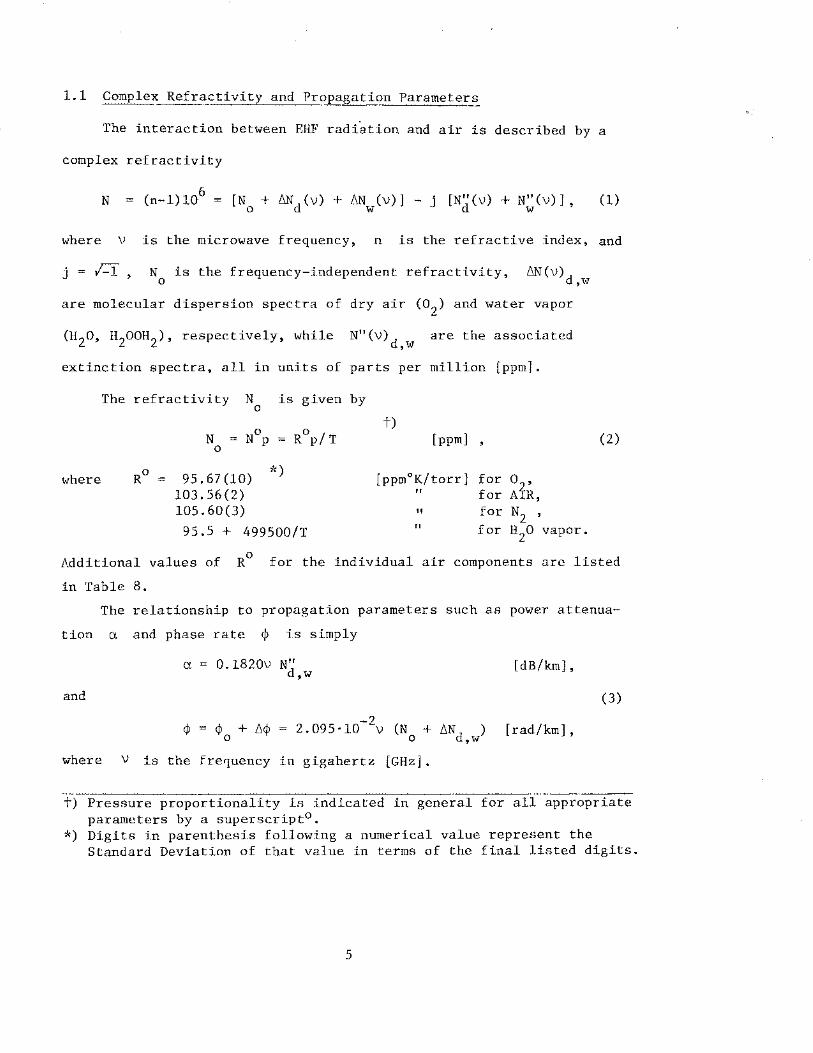
1.1 Complex Refractivity and Propagation Parameters
The interaction between EHF radiation and air is described by a
complex refractivity
N (1)
where v is the microwave frequency, n is the refractive index, and
j r-I '
N is the frequency-independent refractivity, 0
6N(V)d
are molecular dispersion spectra of dry air (02
) and water vapor
N"(v) are the associated d,w
extinction spectra, all in units of parts per million [ppm].
where
The refractivity
N 0
N is given by 0
95.67(10) 103.56(2)
*)
105. 60(3)
t) [ppm]
[ppm°K/torr] " "
for or for A R, for N2 '
,w
95.5 + 499500/T " for H20 vapor.
(2)
Additional values of R0
for the individual air components are listed
in Table 8.
The relationship to propagation parameters such as power attenua
tion a and phase rate ¢ is simply
a = 0.1820v N" d,w [dB/km],
and (3)
¢ = ¢ + 6¢ -2 (N 6Nd ) [rad/km], = 2.095·10 v +
0 0 ,w
where v is the frequency in gigahertz [GHz] .
t) Pressure proportionality is indicated in general for all appropriate parameters by a superscript0 •
*) Digits in parenthesis following a numerical value represent the Standard Deviation of that value in terms of the final listed digits.
5
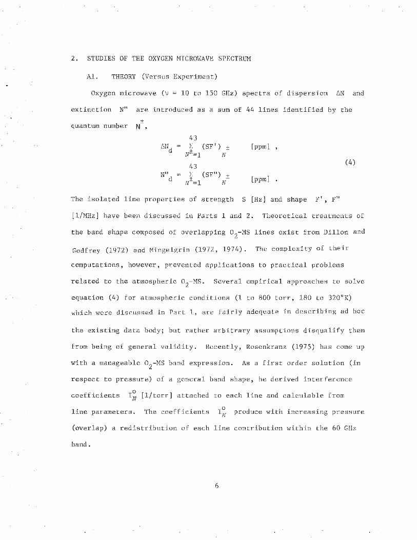
2. STUDIES OF THE OXYGEN MICROWAVE SPECTRUM
Al. THEORY (Versus Experiment)
Oxygen microwave (v = 10 to 150 GHz) spectra of dispersion 6N and
extinction N" are introduced as a sum of 44 lines identified by the
+ quantum number N-,
L!.Nd
N" d
43 L: + N-=1
43
~ N-=1
(SF I) ± [ppm] ' N
(SF") + [ppm] N
.
The isolated line properties of strength S [Hz] and shape F', F"
(4)
[1/MHz] have been discussed in Parts 1 and 2. Theoretical treatments of
the band shape composed of overlapping o2-Ms lines exist from Dillon and
Godfrey (1972) and Mingelgrin (1972, 1974). The complexity of their
computations, however, prevented applications to practical problems
related to the atmospheric o2-Ms. Several empirical approaches to solve
equation (4) for atmospheric conditions (1 to 800 torr, 180 to 320°K)
which were discussed in Part 1, are fairly adequate in describing ad hoc
the existing data body; but rather arbitrary assumptions disqualify them
from being of general validity. Recently, Rosenkranz (1975) has come up
with a manageable o2
-Ms band expression. As a first order solution (in
respect to pressure) of a general band shape, he derived interference
coefficients I~ [1/torr] attached to each line and calculable from
line parameters. The coefficients I~ produce with increasing pressure
(overlap) a redistribution of each line contribution within the 60 GHz
band.
6

The line shape factors for a line within the o2-Ms are given by
(Rosenkranz, 1975)
( 0 0 2 v +v o 1o 2 ) V -V + y I p +Y P F'
\) 0 0
\) 2 0 2 (V +V)2
+ (yop)2 0 (v 0 -v) + (y p)
0
(5)
( 0 0 0 0 ) \) y -(V -V)I y -(v +v)I
F" 0 +
0 p \) 2 0 2 2 0 2
0 (v0-v) +(y p) (v
0+v) +(y p)
(6)
The line strength 0 s = s p remains as defined in Part 1 (Eqs. 7-12;
Tables 3, 7) and Part 2 (Eqs. 18, 19; Table 1). In the vicinity of a
resonance [±(v -v) ~50 MHz] and at lower pressures (p < 100 torr, 0
0 I z 0), the shape factors reduce to
F' =( yv 0 ~ ~ •
(v0-v) +(y p) J o
(7)
The resonant linewidths in o2
are (see Tables 6, 7)
y0 ~ (2.00-0.023N)(300/T) 0 "
9 [MHz/ torr] , ( 8)
whereby the quantum number N dependence is predicted by theory
(Dillon and Godfrey, 1972; Mingelgrin, 1972; Pickett, 1975).
The interference coefficients are calculated as shown by
! 2 d± a 0 2 d± b0
Io = _l_ N+2 N + N~2 N N d± V - V V V
N N N+2 N- N-2
when assuming the following:
i) the nonresonant linewidth in o2
is
y0 = 0.75(300/T) 0 · 9 0
7
- y -0 ( 1 o VN
[MHz/torr]
Rosenkranz (1975),
1 )I (9) 60 GHz j '
(10)
•
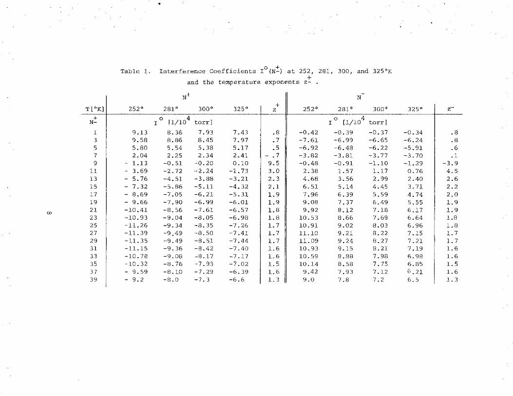
Table 1. Interference Coefficients I0 (N~) at 252, 281, 300, and 325°K + and the temperature exponents z- .
N+ N
T [ °K] 252° 281° 300° 325° +
z 252° 281° 3000 325° I z-+
N-0 4
I [1/10 torr] 0 4
I [1/10 torr]
1 9.13 8.36 7.93 7.43 .8 -0.42 -0.39 -0.37 -0.34 .8 3 9.58 8.86 8.45 7.97 .7 -7.61 -6.99 -6.65 -6.24 .8 5 5.80 5.54 5.38 5.17 .5 -6.92 -6.48 -6.22 -5.91 .6 7 2.04 2.25 2.34 2.41 - .7 -3.82 -3.81 -3.77 -3.70 .1 9 - 1.13 -0.51 -0.20 0.10 9.5 -0.48 -0.91 -1.10 -1.29 -3.9
11 - 3.69 -2.72 -2.24 -1.73 3.0 2.38 1.57 1.17 0.76 4.5 13 - 5.76 -4.51 -3.88 -3.21 2.3 4.68 3.56 2.99 2.40 2.6 15 - 7.32 -5.86 -5.11 -4.32 2.1 6.51 5.14 4.45 3. 71 2.2 17 - 8.69 -7.05 -6.21 -5.31 1.9 7.96 6.39 5.59 4.74 2.0 19 - 9.66 -7.90 -6.99 -6.01 1.9 9.08 7.37 6.49 5.55 1.9
(X) 21 -10.41 -8.56 -7.61 -6.57 1.8 9.92 8.12 7.18 6.17 1.9 23 -10.93 -9.04 -8.05 -6.98 1.8 10.53 8.66 7.69 6.64 1.8 25 -11.26 -9.34 -8.35 -7.26 1.7 10.91 9.02 8.03 6.96 1.8 27 -11.39 -9.49 -8.50 -7.41 1.7 11.10 9.21 8.22 7.15 1.7 29 -11.35 -9.49 -8.51 -7.44 1.7 11.09 9.24 8.27 7.21 1.7 31 -11.15 -9.36 -8.42 -7.40 1.6 10.93 9.15 8.21 7.19 1.6 33 -10.78 -9.08 -8.17 -7.17 1.6 10.59 8.88 7.98 6.98 1.6 35 -10.32 -8.76 -7.93 -7.02 1.5 10.14 8.58 7.75 6.85 1.5 37 - 9.59 -8.10 -7.29 -6.39 1.6 9.42 7.93 7.12 6.21 1.6 39 - 9.2 -8.0 -7.3 -6.6 1.3 9.0 7.8 7.2 6.5 1.3
+-c Q)
u '+'+Q) 0 u Q) u c ~ ~ ~ Q) +c 1---4
10
5
-5
50
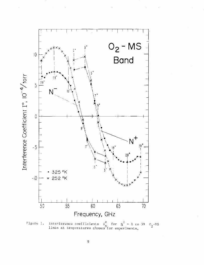
Figure 1.
55 60
0 2 -MS
Band
65 Frequency, GHz
Interference coefficients I0
for N± = 1 to 39 o2-Ms
lines at temperatures chosenNfor experiments.
9

ii) the line coupling elements are obtained by the iterative
procedure (N = 43 to 1),
0
0 y
0 a N-2
0 - a
N
b; ~~~; exp[-2.069(4N-2)/T]
(11)
ii~ the line amplitudes for the + N and the N line branches are
[N(2N+3)/(N+l)(2N+l)] 112 (0.91 to 1),
(12)
[(N+l)(2N-l)/N(2N+l)] 112 (0.82 to 1).
+ Results for between N- = 1 to 39 are listed in Table 1 at four
experimental temperatures and depicted in figure 1. Also given is an
approximate temperature exponent z defined by
I~(T) ~ I~(300)(300/T) 2 • (13)
Frequency and pressure dependencies of equation (4) are expressed
o o 1o. explicitly while the temperature dependence is implicit in S , y ,
Equations (1) to (13) define a theoretical model of the intensity
distribution by the pressure-broadened (p~l to 800 torr) o2-Ms under
atmospheric conditions. One value of 6N or N" is determined, more
or less, by contributions from over thirty lines and their mutual inter-
ferences (Eq. 4). The main purpose of this work is to verify and/or
modify that model by reliable measurements. Experiments start with
finding the parameters (S, y, v ) for as many individual lines as 0
possible. These data are obtained at lower pressures (p < 100 torr).
The next step is to measure at higher pressures (100 to 800 torr) the
band envelope and compare the results first with theoretical predictions
10

based on the linear addition of line.terms (I~= 0) and then find out if
inclusion of interference terms (I~ ~ 0) improves the fit.
A2. EXPERIMENT (Versus Theory)
Quantitative studies are performed using dispersion data from the
PRS (Pressure-Scanning Refraction Spectrometer- Part 2). Conditions
have been simulated as follows:
Pressure -3 3 p = 10 to 10 torr.
Frequency of resonator R2, \) = R
(58 to 62 GHz) ± 5 kHz.
Reference frequency by Rl, \) = vR/2.
Temperature T 252 to 325°K.
Magnetic field strength H ~ 0 and 0 • 53 G •
The variables for experimental and analytical treatments are different
(see below).
Gas
Variable 1
Variable 2
Parameter 1
Parameter 2
Result 1
Result 2
Part A Experiment Prediction
o2, Air, o2 + N2 (Ar, etc.)
Pressure p
Frequency v 0
V = V (1-N p) R
Part B Atmospheric Transfer
Characteristics
AIR
Frequency v
Altitude h
(Pressure p)
Temperature T
Magnetic Field Strength H when
~N(p) = N(VR) - N(VR/2)
a(p) = fct (a1
, Q, B)
and p < 3 torr
a(v)
In part A, experimental data are reduced to line parameters (strengths SN'
widths yN) which in turn are applied to theoretical predictions. The
11
task is completed once a set of parameters can reproduce satisfactorilv
the experimental data. The same set of line parameters is then, of
course, valid for analytical treatments of transfer characteristics as
given in Part B.
2.1 Self-Pressure-Broadening of 0~-MS Lines L.
Pressure-broadening of a line sets limits on pressure and frequency,
2.5 ~ p ~ 100 [torr] and 5 ~ VR ~ 50 [MHz] (14)
The Lorentzian shape (Eq. 7) is valid within these limits; below, Zeeman
and Doppler broadening effects govern the line shape (Section 2.3) and
above, overlapping lines interfere within the o2
-MS band (Section 2.4).
It is impossible to study properties of a pressure-broadened o2-MS
line in absolute isolation since the presence of all lines within the
band adds a continuum term. For conditions specified by equation (14)
one can separate line and continuum cont~ibutions and express equation
(4) through (Eqs. 24 to 27 - Part 2)
and
where
N" d
N" L
2 + (n" - 6vn")p 1 2
and
0 6N + K p ,
L
N" + K"p2
L
(15)
(16)
(17)
Quantitative experimental work relied on dispersion pressure profiles
6N(p). The best candidate to start is the 5+ line, which has the small-
est continuum term (Table 2 - Part 2), K0 (5+) = -1.25 + 0.0170 6v
-3 [10 ppm/torr] at 300°K. So, introducing the theoretical value for
12
K0 (5+) in equation (15) will have the least error in reducing line para-
in case the theoretical strength values
are incorrect.
The pure line dispersion is
0 0 2 (S /y )y/(1 + y )
The pressure is normalized to y = p/p with M
[ppm] • (18)
PM= ±t:.\J/(±y0
- N°\JR)- lt:.\JI/Y0
[torr] (19)
being the pressure at the maximum of t:.NL
!:,~(pM) = So/2yo [ppm] , (20)
and /:,\) = \) - \) [MHz] . (21) 0 R
From figure 2, we realize two important diagnostic values of t:.N(p)
occurring at
The pressure
where
The pressure
p and p ; namely, the maximum t:.N (p ) m o o m
follows from 0
-N = K p L o
p0
= p lA - 1 m ,
and
(22)
(23)
P is shifted in respect to m
as t:.\J changes sign and
is obtained from d(t:.Nd)/dp = 0 (Eq. 15) to be
p = p _/_!_[-A- 2 ±I(A + 4) 2 - 16] m M 'l 2
(24)
(e.g., A= 100, -100, 1, -8 yields pm/pM = .981, 1.021, 0 [min], 6 [max]).
Another diagnostic evolves from dispersion data pairs t:.N(p1
) = t:.N(p2
)
as shown in figure 5.4 of Part 2. The locus of pc = (p1
+ p2)/2 is a
straight line for t:.N:::: 0. 75 t:.N and intersects the peak value t:.N (p ) . o o m
13
For these pairs,
yielding
pc - -26v • 6N/(S0
+ 26vK0
)
pm- PM A/(A + 2)
(25)
(26)
The measured values of pm' p , and p serve as check marks for line 0 c
parameter combinations.
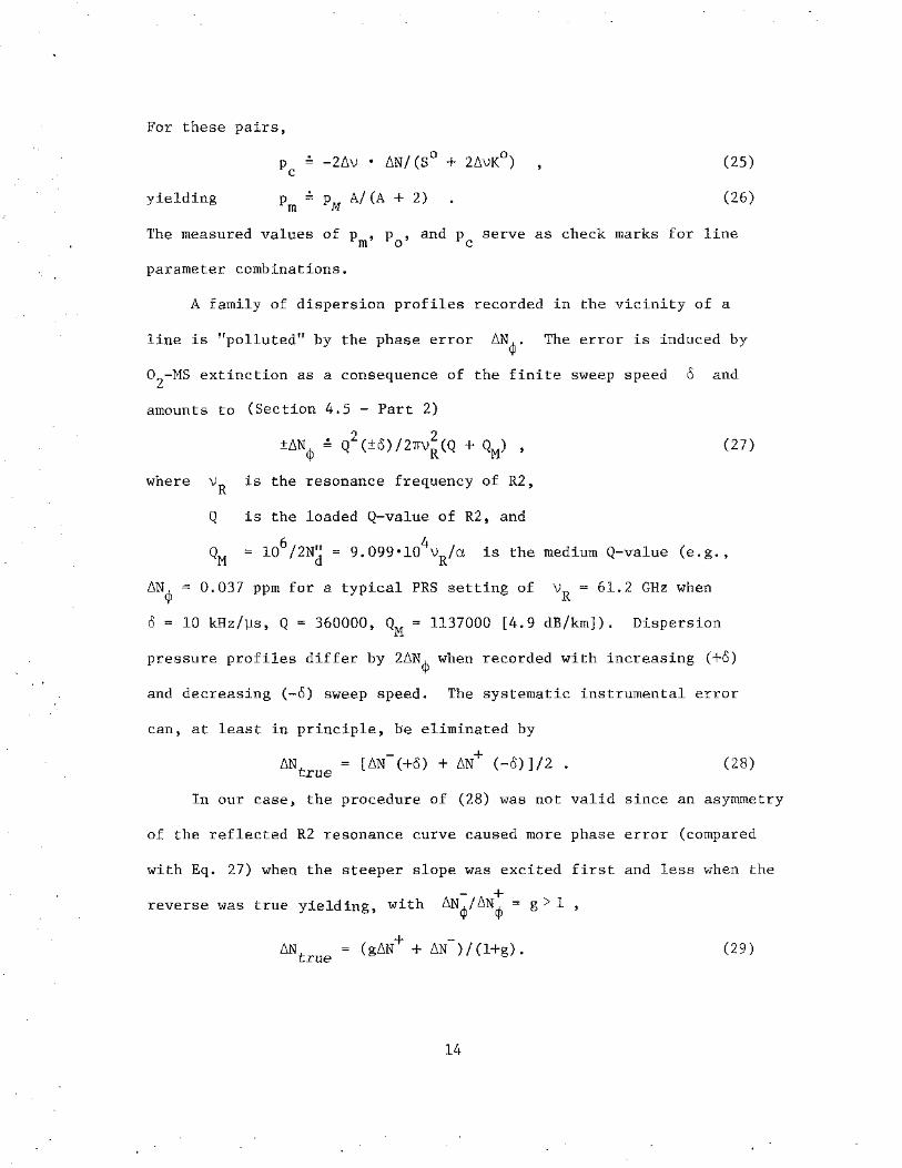
A family of dispersion profiles recorded in the vicinity of a
line is "polluted" by the phase error 6Ncp. The error is induced by
o2
-MS extinction as a consequence of the finite sweep speed 8 and
amounts to (Section 4.5 - Part 2)
(27)
where VR is the resonance frequency of R2,
Q is the loaded Q-value of R2, and
6 4 = 10 /2Nd = 9.099•10 VR/a is the medium Q-value (e.g.,
6Ncp 0.037 ppm for a typical PRS setting of VR = 61.2 GHz when
8 = 10 kHz/~s, Q = 360000, QM = 1137000 [4.9 dB/km]). Dispersion
pressure profiles differ by 26Ncp when recorded with increasing (+o)
and decreasing (-o) sweep speed. The systematic instrumental error
can, at least in principle, be eliminated by
(28)
In our case, the procedure of (28) was not valid since an asymmetry
of the reflected R2 resonance curve caused more phase error (compared
with Eq. 27) when the steeper slope was excited first and less when the
- + reverse was true yielding, with 6Ncp/ Lmcp = g > 1
+ -6Nt = (g6N + 6N )/(l+g). rue (29)
14
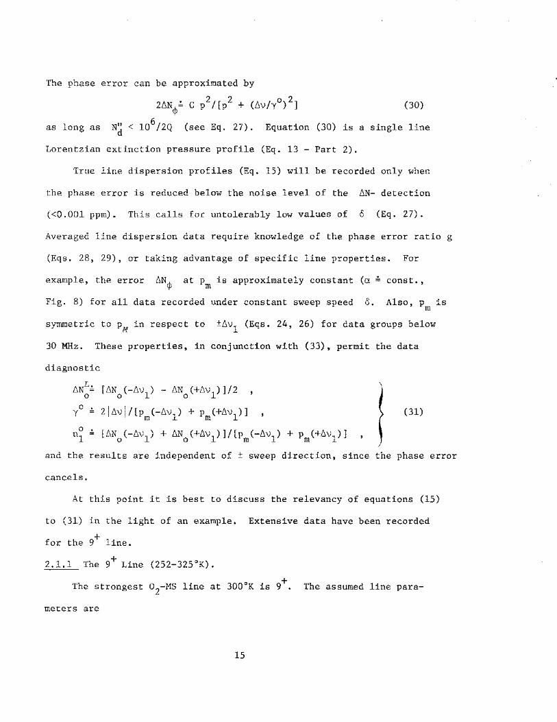
The phase error can be approximated by
26N~~ c p2/[p
2 + (6v/y0
)2
] (30)
as long as N" < l06/2Q (see Eq. 27). Equation (30) is a single line d
Lorentzian extinction pressure profile (Eq. 13- Part 2).
True line dispersion profiles (Eq. 15) will be recorded only when
the phase error is reduced below the noise level of the 6N- detection
(<0.001 ppm). This calls for untolerably low values of 8 (Eq. 27).
Averaged line dispersion data require knowledge of the phase error ratio g
(Eqs. 28, 29), or taking advantage of specific line properties. For
example, the error at p is approximately constant (a~ const., m
Fig. 8) for all data recorded under constant sweep speed 8. Also, p is m
symmetric to pM in respect to ±6v1 (Eqs. 24, 26) for data groups below
30 MHz. These properties, in conjunction with (33), permit the data
diagnostic
6N~~ [6N0
(-6v1
) - 6N0
(+6v1)]/2
yo- 2l6vl/[pm(-6vl) + pm(+6vl)] (31)
and the results are independent of ± sweep direction, since the phase error
cancels.
At this point it is best to discuss the relevancy of equations (15)
to (31) in the light of an example. Extensive data have been recorded
for the 9+ line.
2.1.1 The 9+ Line (252-325°K).
The strongest o2-Ms line at 300°K is 9+. The assumed line para-
meters are
15

N°(300) 0.319 [ppm/torr] (Eq. 2),
\) 61.150567 [GHz] 0
(Table 2 Part 1) '
S0
(300) 1.590 [Hz/ torr] (Table 3 - Part 1) ' w 2.33 (Table 4 Part 1) ' (32)
y0
(300) 1. 79 [:MHz/torr] (Eq.8) u .9 (Eq. 8)
K0
(300) -3 (-3.10 + 0.01176\!)10 [ppm/torr] (Table 2 -Part 2).
Pressure and frequency profiles are predicted for various 6\! and p para-
meters as depicted in figures 2 and 3.
Experimental conditions are identified by (a) the frequency \!R ,
which was tuned symmetrically to \! yielding data in 0
groups
between 5 and 50 :MHz; (b) the temperature T, which was kept constant at
325, 300, 281, or 252°K; (c) the pressure p, which varied betw~en 0 and
150 torr at a rate of roughly ±0.1 torr/second; and (d) the sweep speed ±o
(Eq. 27), which was constant at each T (12 to 15 kHz/~s). Oxygen was of
research quality with a purity of 99.995 percent. Dispersion 6N(p) and
relative attenuation a (p) profiles have been recorded. r
Dispersion Pressure Profiles
+ The body of 9 line data consisted of 190 dispersion profile pairs
+ 6N-(±o) recorded in ±6\!1 groups. Each profile consists of three con-
tributions with various sign combinations:
LineiContinuum Phase Error
+ 6N+ 6N (-6\!1
) 6NL + Ko ap ¢
6N-(-6\!1
) 6NL Ko + + + 6N · g ap ¢ (33) +
~p 6N+ 6N (+6\!1
) -6N + L ¢
6N-(+6\!1
) -6N 0 + + KbP + 6N ·g L ¢
16
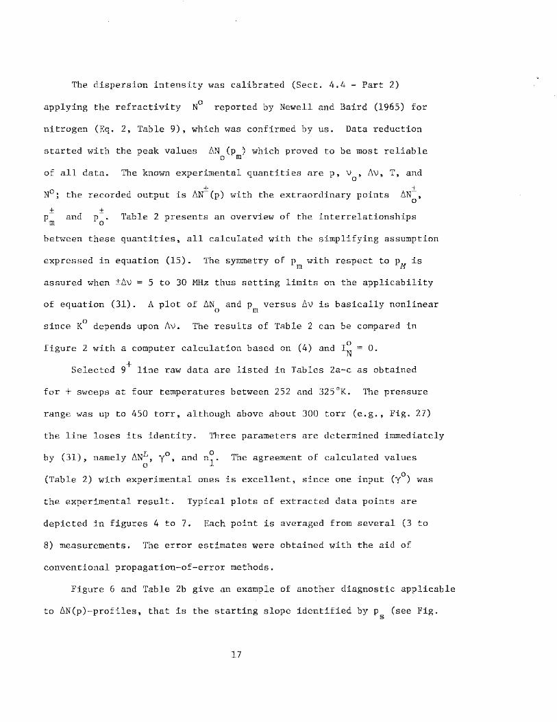
The dispersion intensity was calibrated (Sect. 4.4 - Part 2)
applying the refractivity N° reported by Newell and Baird (1965) for
nitrogen (Eq. 2, Table 9), which was confirmed by us. Data reduction
started with the peak values ~N (p ) which proved to be most reliable o m
of all data. The known experimental quantities are p, v , ~v, T, and 0
+ N°; the recorded output is ~N-(p) with the extraordinary points
and ±
p • 0
Table 2 presents an overview of the interrelationships
between these quantities, all calculated with the simplifying assumption
expressed in equation (15). The symmetry of pm with respect to pM is
assured when ±~v = 5 to 30 MHz thus setting limits on the applicability
of equation (31). A plot of ~N and p versus ~v is basically nonlinear o m
since K0 depends upon ~v. The results of Table 2 can be compared in
figure 2 with a computer calculation based on (4) and I0 = 0. N
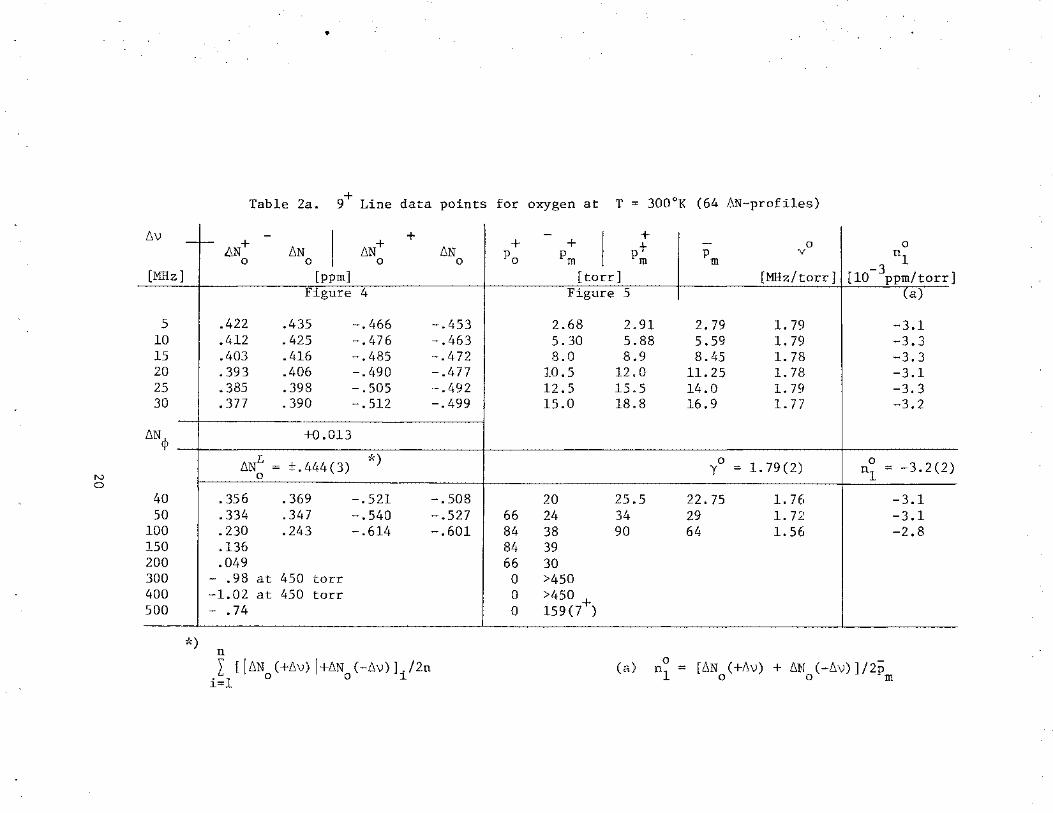
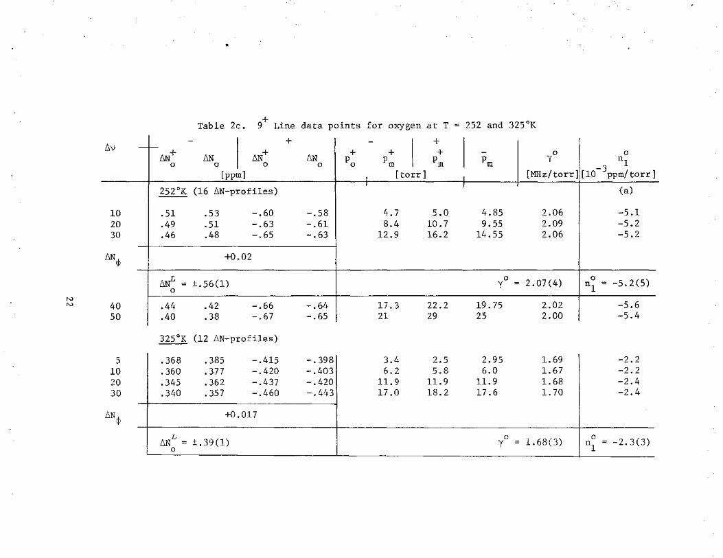
Selected 9+ line raw data are listed in Tables 2a-c as obtained
for + sweeps at four temperatures between 252 and 325°K. The pressure
range was up to 450 torr, although above about 300 torr (e.g., Fig. 27)
the line loses its identity. Three parameters are determined immediately
by (31), namely ~N~, y 0, and n~. The agreement of calculated values
(Table 2) with experimental ones is excellent, since one input (y0
) was
the experimental result. Typical plots of extracted data points are
depicted in figures 4 to 7. Each point is averaged from several (3 to
8) measurements. The error estimates were obtained with the aid of
conventional propagation-of-error methods.
Figure 6 and Table 2b give an example of another diagnostic applicable
to ~N(p)-profiles, that is the starting slope identified by p (see Fig. s
17

2.1- Part 2). It follows that for a Lorentzian shape plus a pressure-
linear continuum term (Eq. 15)
(34)
transforming to the approximation (A>>l)
(35)
that supports a line width parameter. An example is given in Table 2b.
+ The simple concept of assuming 6N~
+ canst. for 6N- and taking
0
advantage of the line symmetry (Eq. 31) yields correct line parameters,
although only one data point out of many is utilized. A computer program
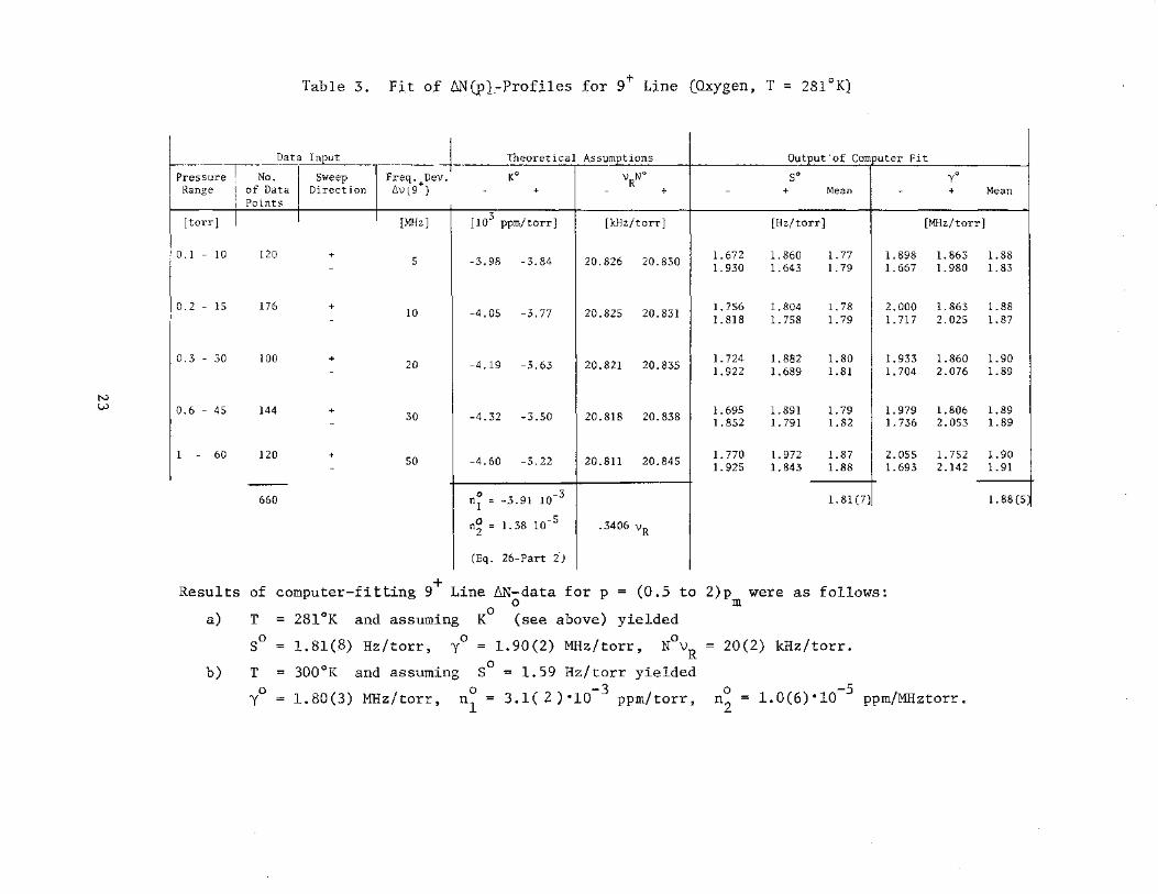
was written to adjust and 0 y to give the best fit in the least
squares sense to a large number of 6N+(p) or 6N-(p) data points.
Unfortunately, the program did not converge to unique values of S0 and
y0 as evident from the example listed in Table 3. The large fluctuations
are caused by the phase error 6N¢ (Eq. 22), which distorts 6N(p)-profiles
in a systematic way. Such analysis, however, is still useful in that
the mean of each parameter agrees reasonably well with the more reliable
values deduced from
The analysis demonstrated in Tables 2a-c was also performed on the
6N-(p-) data and the results were essentially the same with slightly o m
larger error margins due to the larger phase error (e. g.'
Figs. 4, 7).
In summary, it is possible to deduce g+ line parameters from disper-
sion pressure profile maxima without paying attention to the phase error
+ 6N¢· The uncertainty (standard deviation from the mean) was 0.7, 1.1,
and 6 percent for 6~, y0 and n°
1, respectively, for the data at 281
0 '
18
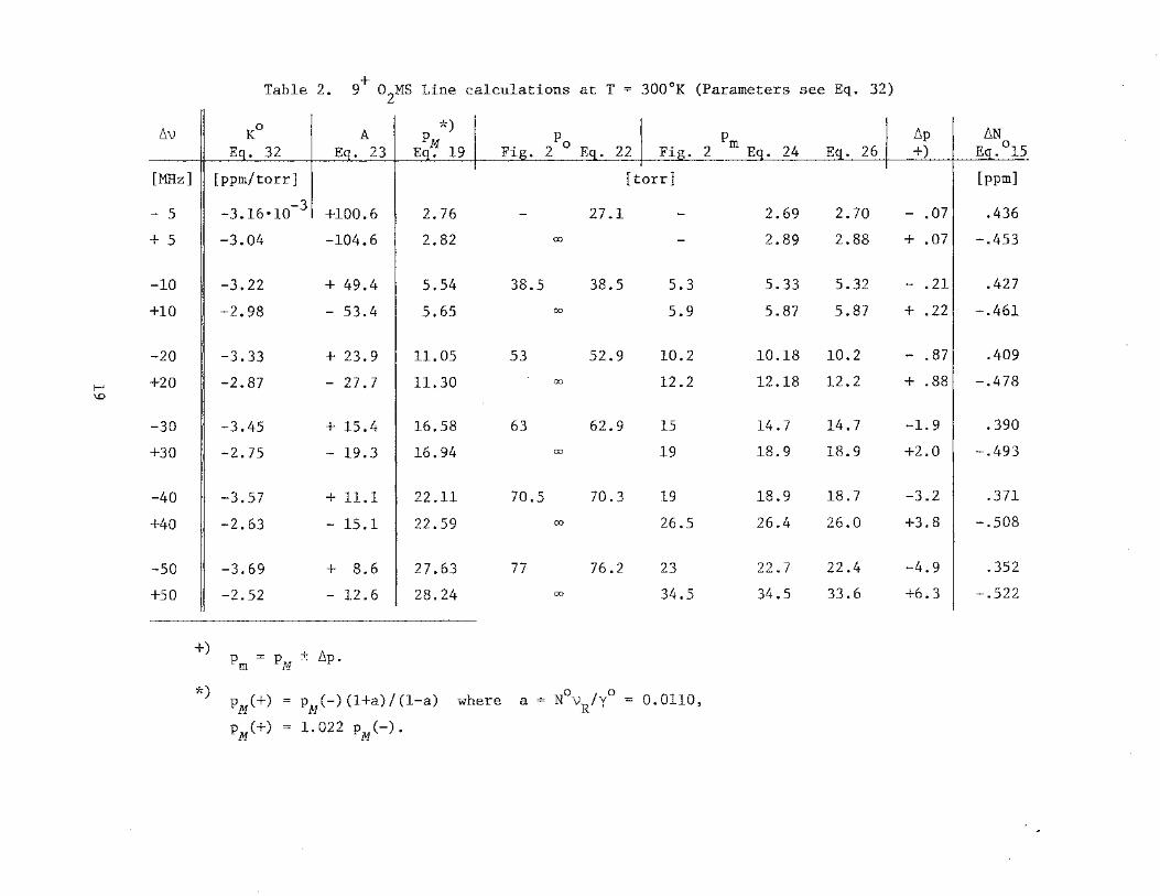
Table 2. 9+ o2
MS Line calculations at T = 300°K (Parameters see Eq. 32)
6v II Ko 6p 6N E • 32 +) E . 0 15
[MHz] II [ppm/torr] [torr] [ppm]
- 5
II
-3.16•10-31 +100.6 2.76 - 27.1 - 2.69 2.70 - . 07 .436
+ 5 -3.04 -104.6 2.82 00 - 2.89 2.88 + .07 -.453
-10
II -3.22 + 49.4 5.54 38.5 38.5 5.3 5.33 5.32 - .21 .427
+10 -2.98 - 53.4 5.65 00 5.9 5.87 5.87 + .22 -.461
-20 -3.33 + 23.9 11.05 53 52.9 10.2 10.18 10.2 - .87 .409
1-' +20 -2.87 - 27.7 11.30 00 12.2 12.18 12.2 + .88 -.478 \.0
-30 -3.45 + 15.4 16.58 63 62.9 15 14.7 14.7 -1.9 .390
+30 -2.75 - 19.3 16.94 00 19 18.9 18.9 +2.0 -.493
-40 -3.57 + 11.1 22.11 70.5 70.3 19 18.9 18.7 -3.2 .371
+40 -2.63 - 15.1 22.59 00 26.5 26.4 26.0 +3.8 -.508
-50 -3.69 + 8.6 27.63 77 76.2 23 22.7 22.4 -4.9 .352
+50 -2.52 - 12.6 28.24 00 34.5 34.5 33.6 +6.3 -.522
+) p = p ± 6p. m M
*) pM(+) = pM(-)(l+a)/(1-a) where o I o a = N VR y = 0.0110,
pM(+) = 1.022 pM(-).
N 0
t.v
[MHz]
5 10 15 20 25 30
L'.N¢
40 50
100 150 200 300 400 500
-
ic)
.,
Table 2a. 9+ Line data points for oxygen at T = 300°K (64 L'.N-profilE~s)
-
I + -
I +
1-- LlN+ L'.N+ + + p+ - 0 0 L'.N L'.N Po Pm pm y nl 0 0 0 0 m
-3 [ppm] [torr] [MHz/torr] [10 ppm/torr] Figure 4 Figure 5 (a)
.422 .435 -.466 -.453 2.68 2.91 2. 79 1. 79 -3.1
.412 . 425 -.476 -.463 5.30 5.88 5.59 1. 79 -3.3
.403 .416 -.485 -.472 8.0 8.9 8.45 1. 78 -3.3
. 393 .406 -.490 -.477 10.5 12.0 11.25 1. 78 -3.1
.385 . 398 -.505 ·-.492 12.5 15.5 14.0 1. 79 -3.3
.377 .390 -.512 -.499 15.0 18.8 16.9 1.77 -3.2
+0.013
L'.NL = ±.444(3) *) 0 = 1. 79(2) 0
0 y n1 = -3.2(2)
• 356 .369 -.521 -.508 20 25.5 22.75 1. 76 -3.1 .334 .347 -.540 -.527 66 24 34 29 1.72 -3.1 .230 .243 -.614 -.601 84 38 90 64 1. 56 -2.8 .136 84 39 .049 66 30
- .98 at 450 torr 0 >450 -1.02 at 450 torr 0 >450 - .74 0 159(7+)
- ----- ------- ------- - -- ---
n I [jl'.N (+L'.v) J+t.N (-L'.v)]./2n
. 1 0 0 l l=
(a) 0 -n1 = [L'.N (+L'.v) + L'.N (-L'.v)]/2p o o m

N }-1
6v _ 1--
[MHz]
5 7.5
10 15 20 25 30
6Ncp
35 40 45 so
100 150 200
-
Table 2b. 9+ Line data points for oxygen at T = 281°K (98 6N-profiles)
+ Average 0 - - + y = - + 6N+ 6N 6N+ 6N + + + - 6v/p + 0
0 0 0 Po pm pm Pm m ps nl
[ppm] [torr] [MHz/torr] [torr] -3 [10 ppm/torr] Figure 6 (a)
.441 .464 -.503 -.480 23 2.54 2. 72 2.63 1. 90 1. 32 1. 35
.435 .458 -.512 -.489 28 3.8 4.1 3.95 1.90 -3.9
.432 .455 -.518 -.495 31 4.8 5.4 5.2 1. 92 2.68 2.70 -3.8
.422 .445 -.528 -.505 7.0 8.6 7.8 1. 92 -3.8
.413 .436 -.536 -.513 46 9.5 11.3 10.4 1.92 5.35 5.29 -3.7
.407 .430 -.546 -.523 11.9 14.3 13.1 1.91 -3.6
. 395 .418 -.554 -.531 57 13.8 17.8 15.8 1. 90 8.36 7.86 -3.6
+0.023
6NL = ±0.474(3) 0 1.90(4) *) 0
r = 1. 91(2) '
n1 =-3.7(2) 0
.380 .403 -.559 -.537 15.5 21.8 18.65 1.88 -3.6
. 372 .395 -.566 -.543 65 17.2 25.5 21.35 1. 87 11.1 10.5 -3.5
. 365 .388 -.574 -.551 19.5 29.0 24.25 1. 86 -3.4
.355 .378 -.579 -.556 72 21 33 27 1. 85 13.8 12.8 -3.3
.217 -.68 87 35 80 57.5 1. 74
.137 83 40
.046 58 29 -- --··
*) Analyzed with equation (35) and averaged by [y0 (+6v) + y0 (-6v)]/2
N N
t:.v
10 20 30
b.N¢
40 50
5 10 20 30
b.N¢
- ~
..
+ Table 2c. 9 Line data points for oxygen at T = 252 and 325°K
- + - + b.N+ t:.N b.N+ b.N
+ + + - 0
0 0 0 0 Po Pm pm pm "{
[ppm] I
[torr] I [MHz/torr]
252°K (16 b.N-profiles) I I
.51 .53 -.60 -.58 4.7 5.0 4.85 2.06
.49 .51 -.63 -.61 8.4 10.7 9.55 2.09
.46 .48 -.65 -.63 12.9 16.2 14.55 2.06
+0.02
t:.rf = ±.56(1) 0 = 2.07(4)
0 "{
.44 .42 -.66 -.64 17.3 22.2 19.75 2.02
.40 .38 -.67 -. 65 21 29 25 2.00
325°K (12 b.N-profiles)
.368 .385 -.415 -. 398 3.4 2.5 2.95 1.69
. 360 . 377 -.420 -.403 6.2 5.8 6.0 1. 67
.345 .362 -.437 -.420 11.9 11.9 11.9 1. 68
.340 . 357 -.460 -.443 17.0 18.2 17.6 1. 70
+0.017
t:.NL = ±.39(1) 0 = 1. 68(3) y 0
0 nl
-3 [10 ppm/torr]
(a)
-5.1 -5.2 -5.2
0 n1 = -5.2(5)
-5.6 -5.4
-2.2 -2.2 -2.4 -2.4
0 n
1 = -2. 3(3)
N I.J..l
Table 3. F;i,t of b.N(pl_-Profj,les for 9+ Line (Oxygen, T :::: 281 °K)
Data Input ------~-- Theoretical Assumptions -------r-----Pressure No. Sweep Freq. Dev. Ko VRN° Range of Data Direction L\v(9+) - + - +
Points
[torr] [MHz] 3 [10 ppm/torr] [kHz/torr]
0.1- 10 120 + 5 -3.98 -3.84 20.826 20.830 -
0.2 - 15 176 + 10 -4.05 -3.77 20.825 20.831 -
0.3 - 30 100 + 20 -4.19 -3.63 20.821 20.835 -
0.6 - 45 144 + 30 -4.32 -3.50 20.818 20.838 -
1 - 60 120 + so -4.60 -3.22 20.811 20.845 ----
660 0 -3 n1 = -.3.91 10
0 -5 n2 = 1.38 10 . 3406 vR
(Eq. 26-Part iJ
Results of computer-fitting 9+ Line ~N-data for p = (0.5 to 0
a) T = 281°K and assuming Ko (see above) yielded 0 0 = 1.90(2) MHz/torr,
0 S = 1.81(8) Hz/torr, y N VR
b) T = 300°K and assuming S0 = 1.59 Hz/torr yielded
0 = 1.80(3) MHz/torr, 0 -3
y n1
= 3.1( 2) •10 ppm/torr,
- Ou1:£_ut 'of Comr_uter Fit so
- + Mean -
fHz/torr]
1.672 1.860 1.77 l. 898 1.930 1.643 l. 79 1.667
l. 756 1. 804 l. 78 2.000 l. 818 1.758 l. 79 l. 717
l. 724 l. 882 l. 80 l. 933 1.922 1.689 l. 81 1.704
1.695 l. 891 l. 79 1.979 l. 852 1. 791 1. 82 1.736
1. 770 l. 972 1. 87 2.055 1.925 1.843 l. 88 1.693
1.81 (7)
2)p were as follows: m
20(2) kHz/torr.
Yo +
[MHz/torr]
l. 863 1.980
1.863 2.025
1.860 2.076
1.806 2.053
1.752 2.142
0 -5 n2
= 1.0(6)•10 ppm/MHztorr.
Mean
1.88 1.83
l. 88 1.87
l. 90 1.89
l. 89 1.89
l. 90 l. 91
l. 88 (5

and 300°K. The error margins are about double at 252 and 325°K since
the number of individual ~N-profiles was smaller.
The Phase Error
+ The phase error at pm appears as a discontinuity 2~N~ at
+ ~v 0 in a plot of ~N--vs-~v (e.g., Fig. 4). Tne error ratio g
(Eq. 29) is determined by the offset. The ratio g is also found in
+ ~N-(p)-profiles recorded at ~v = 0. Here, the line contribution is
zero (Eq. 18) and the continuum term is offset by (e.g.,
Fig. 7). The ratio g remains constant, at least for pressures up to
100 torr (Fig. 7). The operation of (29) can now be performed upon the
+ recorded data ~N-(p) which then are treated as true molecular information.
+ The functional form of ~N~(p) is proportional to o2-Ms attenuation
a (Eq. 27, Fig. 8). The line attenuation dominates when p < p and m
equation (30) is a good approximation. The constant C is determined
by averaging the "C of best fit" for the differences + -~N - ~N (~.g.,
Fig. 5.6- Part 2). The value of C was constant to within 4 percent
+ for ±~v(9 ) = 5 to 30 MHz. With C known, it is possible to reconstruct
~N(p) from ~N+(p) and vice versa.
Obviously, the phase error ~N¢ can be reduced by slower sweep
speeds o (Eq. 27). The first PRS design, however, did not permit
operation below o ~ 11 kHz/~s. A new digital phase meter has just been
completed (APPENDIX C) that can be operated as low as 1.5 kHz/~s with a
detection sensitivity of ~N . < 0.004 ppm. ml.n An example is shown in
figure 14. The error at reduces hereby from 0.24 ~N 0
o = 11.4 kHz/~s (Fig. 12) to 0.035 ~N at o = 1.52 kHz/~s 0
according to the ratio of o. 24
at
Attenuation Pressure Profiles
The theoretical profiles are expressed through equations (3), (4),
(6). An example for the 9+ line, which assumes I~= 0, is depicted in
figure 8. A comparison of attenuation a and dispersion ~N favors
the latter for line studies, the reason being that a(p) lacks extraordinary
points and a distinction between + and - ~V data.
The peak detector at VR generates a voltage a1
(APPENDIX C,
+ Fig. Al) simultaneously with ~N-(p)-profiles. The voltage a
1 relates
to attenuation a by (Eqs. 39, 29 - Part 2)
(36)
The relation between al and a requires knowledge of the detector law
S and the effective length LR(Q), both of which are very difficult to
measure accurately. The best we were able to achieve was ± 5 percent
for Q and ± 10 percent for S. This accuracy cannot compete with the
dispersion results.
Various biased and unbiased point-contact and Schottky-barrier
diodes have been employed at VR with conversion efficiencies between
80 and 400 mV/mW. The detection law varied between S = 1.0 and 1.5
since the diode is always subjected to the full reflected power (0.5 to
5 mW).
Table 4 and figure 9 exhibit two examples of attenuation pressure
profiles, just to demonstrate the difficulties of any undertaking to
obtain absolute data. The first is a result of fitting 9+ pressure
profiles a [a =a1
(p), but calibrated in decibel with precision attenuator] X X
to the expression {Eq. 32 - Part 2)
25

PREDICTION . . 0.4 g+ 02
300°K 0.3
Io = 0 N
0.1
E 0.1 a. a. . z <l
----c /---0 (/) -0.1
nop ----.... 1 --<l.l
a. 6v(;+J-= (/)
0 -0.1
-0.3
-0.4
-0.5
0 20 40 60 80 100 Pressure, torr
Figure 2. o2-MS dispersion pressure profiles around the 9+ Line as predicted for detection by the PRS.
o._ o._
z <1
0.4
c -0.2 0 (/) '--
~ -0.4 r---..: __ _ i:5
-100 -80 -60 -40 -20 0 20 40 60 80 100
Frequency Deviation 6v, M Hz
Figure 3. Calculated frequency profiles for the 9+ o2-Ms Line at 10, 40, and 150 torr (Mingelgrin, 1972). Assumed was y 0 = 1.95 MHz/torr (Table 7).
26

E 0.55 a.. a..
0
~ 0.50
c 0 (/)
Qj 0.45 a.. (/)
0 E :J
E >< 0 2
Figure 4.
30
Measured peak dispersion (see Table 2a) .
6N in vicinity of 9+ Line 0
---· --· --· --·--. ___.-f.[/1-
'\, -·---·----- Dispersion+ ~~/· / ~·
"- 0 ( +) Phase Error'v'/// /
:: 20 , "-/Y ~.--·--· ?/ ~~,- -- f/ 0
+E 0.. ~-- - //
,e-_ .. -· _/' -//V'
~~ _____.__. r o;specs;on ' ,. /
Frequency Deviation 6-v , M Hz
oL-~~--L-~-L~--L--L~~L-~-L--L-~-L~--~~~~
-50 - 40 -30 - 20 -I 0 0 I 0 2 0 30 40 50
Figure 5. Meas¥red pressure p~ at peak dispersion 6N of 9 Line (see Table 2a) . 0
in vicinity of
27
I N 50 /-/ X I ~
40 281 °K ~ //" <J c 0 30 ....
~ 0 ·:; OJ
-~ ~+~v 0 20 >-
/ - ~ZI (,)
c OJ ::J 10 c-OJ ·' ... < LL
0 0 5 10 15
Pressure p5
, torr
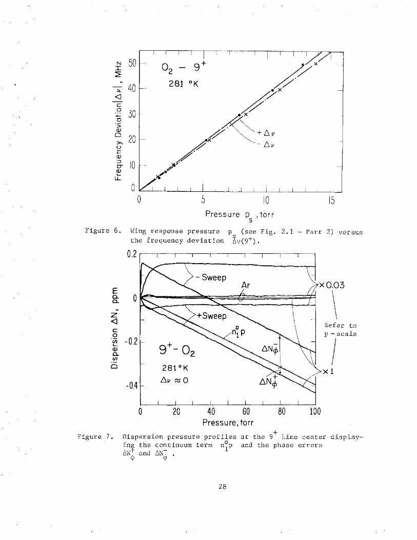
Figure 6. Wing response pressure p (see Fig. 2.1 - Part 2) versus the frequency deviation ~v(9+).
E c. c. ~
z <]
c .Q
"' '-OJ c. "' 0
Figure 7.
0
-0.2
-0.4
0 20 40 60 Pressure, torr
80
X0.03
100
\ Refer to p- scale
I Xi
Dispersion pressure profiles at the 9+ Line center displayin~ the continuum term n~p and the phase errors f.I.N¢ and f.I.N~ .
28
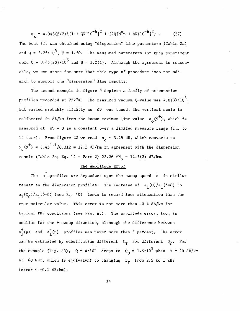
The best fit was obtained using "dispersion" line parameters (Table 2a)
5 and Q = 3.25•10 , 8 = 1.20. The measured parameters for this experiment
5 were Q = 3.45(20)•10 and 8 = 1.2(1). Although the agreement is reason-
able, we can state for sure that this type of procedure does not add
much to support the "dispersion" line results.
The second example in figure 9 depicts a family of attenuation
profiles recorded at 252°K. 5 The measured vacuum Q-value was 4.0(3)•10 ,
but varied probably slightly as ~V was tuned. The vertical scale is
calibrated in dB/km from the known maximum line value a (9+), which is 0
measured at ~V = 0 as a constant over a limited pressure range (1.5 to
15 torr). From figure 22 we read a = 3.45 dB, which converts to 0
12.5 dB/km in agreement with the dispersion
result (Table 2c; Eq. 14 - Part 2) 22.26 ~N = 12.5(2) dB/km. 0
The Amplitude Error
+ The a1-profiles are dependent upon the sweep speed o in similar
manner as the dispersion profiles. The increase of a1 (Q)/a1 (o=O) to
a1 (QG)/a1 (o=O) (see Eq. 40) tends to record less attenuation than the
true molecular value. This error is not more than -0.4 dB/km for
typical PRS conditions (see Fig. A3). The amplitude error, too, is
smaller for the + sweep direction, although the difference between
a1(p) and a~(p) profiles was never more than 3 percent. The error
can be estimated by substituting different
the example (Fig. A3), 5 Q = 4•10 drops to
fT for different QG. For
5 QG = 1.6•10 when a = 20 dB/km
at 60 GHz, which is equivalent to changing fT from 2.5 to 1 kHz
(error< -0.1 dB/km).
29

Table 4.
L1v(9+)
a p X
[torr]
0 0 3 .20 6 .62 9 1.02
12 1.33 15 1. 55 18 1. 70 21 1.80 24 1.88 27 1.93 30 1.99
Example of Fitting Attenuation Pressure Profiles in the Vicinity of the 9+ Line (T = 300°K, o2).
-20 MHz -30 MHz
a *) Differ. a a *)
Differ. c a- a X c a- a
X c X c
[dB] [%] [dB] [%]
0 0 0 0 0 .186 7.0 .10 .009 2 .591 4.7 .35 .328 6.3 .995 2.5 .65 .625 3.9
1.308 1.7 .96 .919 4.3 1.535 1.3 1. 22 1.175 3.7 1. 695 .3 1.42 1.385 2.5 1.809 - .5 1.57 1.554 1.0 1.892 - .6 1. 70 1.689 . 7 1.925 - . 3 1. 80 1.794 .3 2.001 - .5 1.88 1.879 .1
*) Calculated attenuation using the experimental parameters
Q = 325,000 and s = 1. 20,
and the 9+ l1'ne t parame ers:
S0 = 1. 59 Hz/torr, y 0 = 1. 79 MHz/torr, and K" (see Eq. 26 of Part 2).
30

Figure 8.
PREDICTION 12 -
\
E - 0 X.
' cg 8 -
c 0
0 :::J c Q)
<(
r:Q '"d ~
.....t C'd
c .Q 0 :::J c 2 <(
Q)
> -0 Q)
0::
Pressure, torr
20 40
02-MS attenuation pressure predicted for detection by
2
3
60 80 100
+ profiles around the 9 Line as the PRS.
Pressure, torr
0 6 12 18 30
Figure 9. Recorded attenuation pressure profiles for the 9+ Line. Effective path length LR== 0.312 km; detection law p~1.1. Also, see figure 22.
31
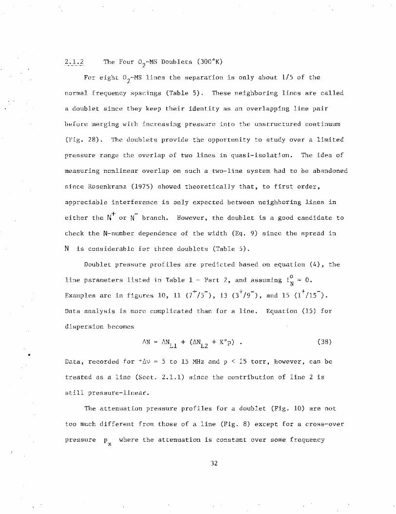
2.1.2 The Four o2-Ms Doublets (300°K)
For eight o2-Ms lines the separation is only about 1/5 of the
normal frequency spacings (Table 5). These neighboring lines are called
a doublet since they keep their identity as an overlapping line pair
before merging with increasing pressure into the unstructured continuum
(Fig. 28). The doublets provide the opportunity to study over a limited
pressure range the overlap of two lines in quasi-isolation. The idea of
measuring nonlinear overlap on such a two-line system had to be abandoned
since Rosenkranz (1975) showed theoretically that, to first order,
appreciable interference is only expected between neighboring lines in
+ -either the N or N branch. However, the doublet is a good candidate to
check the N-number dependence of the width (Eq. 9) since the spread in
N is considerable for three doublets (Table 5).
Doublet pressure profiles are predicted based on equation (4), the
line parameters listed in Table 1 - Part 2, and assuming I~ = 0.
Examples are in + - + - + -figures 10, 11 (7 /5 ), 13 (3 /9 ), and 15 (1 /15 ).
Data analysis is more complicated than for a line. Equation (15) for
dispersion becomes
~N (38)
Data, recorded for ±~v = 5 to 15 MHz and p < 15 torr, however, can be
treated as a line (Sect. 2.1.1) since the contribution of line 2 is
still pressure-linear.
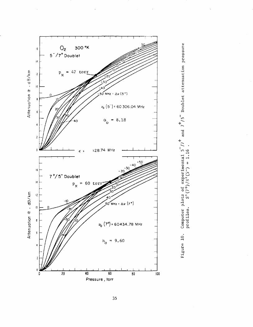
The attenuation pressure profiles for a doublet (Fig. 10) are not
too much different from those of a line (Fig. 8) except for a cross-over
pressure px where the attenuation is constant over some frequency
32

+ -range (~40 MHz in the 7 /5 example). Experimentally, the pressure px
can serve as check point for the validity of a theoretical prediction,
even when the data (Eq. 36) are recorded as relative attenuation.
The dispersion pressure profiles are significantly different in the
vicinity of one or the other line (Fig. 11).
displays two extraordinary points, ~N0 (pm)Ll The doublet dispersion
and L2 ~N (p ) , that are o m
sensitive to the width parameter of line 1 and 2, respectively. A wrong
value of in the prediction will cause noticeable discrepancies with
the experimental data. The profile at ~V = 0 is, up to 100 torr,
mostly the contribution from the other partner in the doublet. The
+ -3 /9 doublet is well suited to study N-dependence of the linewidth.
Predictions that assumed the same width parameter (1.79 MHz/torr) for
both lines did not agree with measured data.
Results
+ - + -Recorded dispersion profiles for 7 /5 and 3 /9 , which were restricted
in ±~v (5 to 15 MHz) and p (< 15 torr), have been analyzed for line
parameters. Data analysis was by equation (31), and.the results are
summarized in Table 5. The same phase error problem existed as for the
9+ line. Two examples (Figs. 12 and 14) are representative of details
of many individual data runs. The 7+/5- averaged data points agree well
with predictions based upon equations (4), (7), (8), and I 0 = 0. N
Deviations from a pressure-linear overlap of the two doublet lines are
not detectable. This finding is supported by the pressure p0
that is
kind of a balance point between the two line contributions.
33

+ ·-Very recent results on the 3 /9 doublet profitted from smaller
phase errors due to reduced sweep speeds o possible with the new phase
meter (APPENDIX C). It can operate at a sampling rate fT =1kHz. For
the example, figure 14, the low Q mode of R2 (Sect. 3.5.2 - Part 2) was
used. The reduction in phase error is significant, especially when
compared with figure 12. The slight positive slope of the N2-baseline
is caused by a sloping power mode of the doubler generating VR = 58.4 GHz
(Eq. 64 - Part 2) that was later avoided by more careful tuning and by
operating with less sweep width in the high Q mode.
Under any circumstance, it is of advantage to operate the PRS at
the highest Q-values that possibly can be achieved. The reason for this
is that the two competing requirements of low sweep speed and sufficient
sweep width have to be met by observing (Eqs. 36, 52 - Part 2)
(39)
where
(VR in GHz, a in dB/km from figures 8, 10, 11, 13, 15, etc). This
adjustment causes the R2 resonance curve to be swept to ten times its
bandwidth, which assures minimum phase and amplitude detection errors.
+ - + -Although the number of observations made on the 7 , 5 , 3 , 9
lines are not enough for indisputable conclusions, the results (Table
5) do support two assertions: i) the line width depends upon the quantum
number N (Gardiner et al., 1975) and ii) the strengths agree
within 5 percent with the theoretical values.
34
Q)
16 02 300 OK H :::! (fJ
5- /1+ Doublet (fJ Q)
H 14 p.
!=l 0
E px •r-i
.:£ 12 ·- -1-1 ........ Ctl m g "0 Q)
10 -1-1 -1-1 a Ctl
c -1-1 0 Q)
r-l 0 ,.0 ::J v0 (5-) = 60 306.04 MHz :::! c 0 2 ~ ...... <( I
a 8.18 ll"\ -0 + r--
'U !=l Ctl
+ r---128.74 MHz I
E ll"\ \0 r-l
r-l . Ctlr-l -1-1 !=l II Q)
16 s.....-..
•r-i I
7+/5- Doublet Hll"l GJ'-' p.o
14 Kr:fl
p = Q)-
X ......... 4-l+ or--
E ......... .:£ 12 (flO
' -1-!Cf}
m 0 "0
r-l p.
10 . H (fJ
a Q) Q) -1-lr-l
c :::! •r-i 0 P.4-l
...... v0 (7+) = 60434.78 MHz s 0 0 0 H ::l UP. c Q) ...... ...... <( 0
ao = 9.60 r-l
Q)
H :::! bO
·r-i ~
0 0 20 80 100
Pressure, torr
35
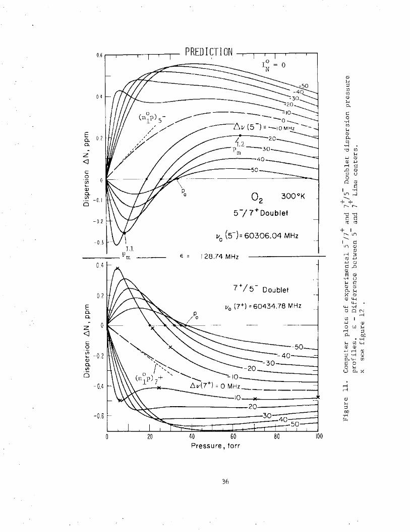
0.6 PREDICTION I I
0
Q) 1-1 ::l C/J
0.4 C/J Q)
1-1 0..
(j 0
·r-1 {_I)
1-1 E 0.2
Q)
a. 0..
a. C/J •r-1 .
~ "0 C/J
z 1-1
<J 4J Q) Q) 4J
.-! (j
c ,.0 Q)
0 ::l C)
·u; 0 0 Q Q) ... (j
Q) I •r-1 a.
02 300°K Lf'),_:j (/)
-0.1 -0 ++ " " 5 -; 7+ Doublet "0"0
-0.2 0 0 Cll Cll
110
(5-)= 60306.04 MHz + I
" Lf')
-0.3 -I 0 Ll Lf') Q)
Q)
pm E = 128.74 MHz .-! :.: Cll 4J
0.4 4J Q) Q,.O Q) s Q)
·r-1 C)
7 +I 5- Doublet 1-1 0 Q) Q) 0..!-1
0.2 ~ Q) a.lll-l
E 110
(7+) = 60434.78 MHz 4-l 4-l ·r-1
a. OQN a. .-!
C/J I
0 4J Q)
z 0 w 1-1
<J .-! ::l 0.. bJ)
• •r-1 c 1-1 C/J 4-l 0 Q) Q)
~ -0.2 4-l.-!Q) ::l •r-f Q)
Q) 0.. 4-l C/J a. s 0 (/) 0 1-1
0 u 0.. ~
. -0.4 .-!
.-!
Q)
20 1-1 ::l
-0.6 bJ)
·r-1
""' 0 20 40 60 100
Pressure, torr
36
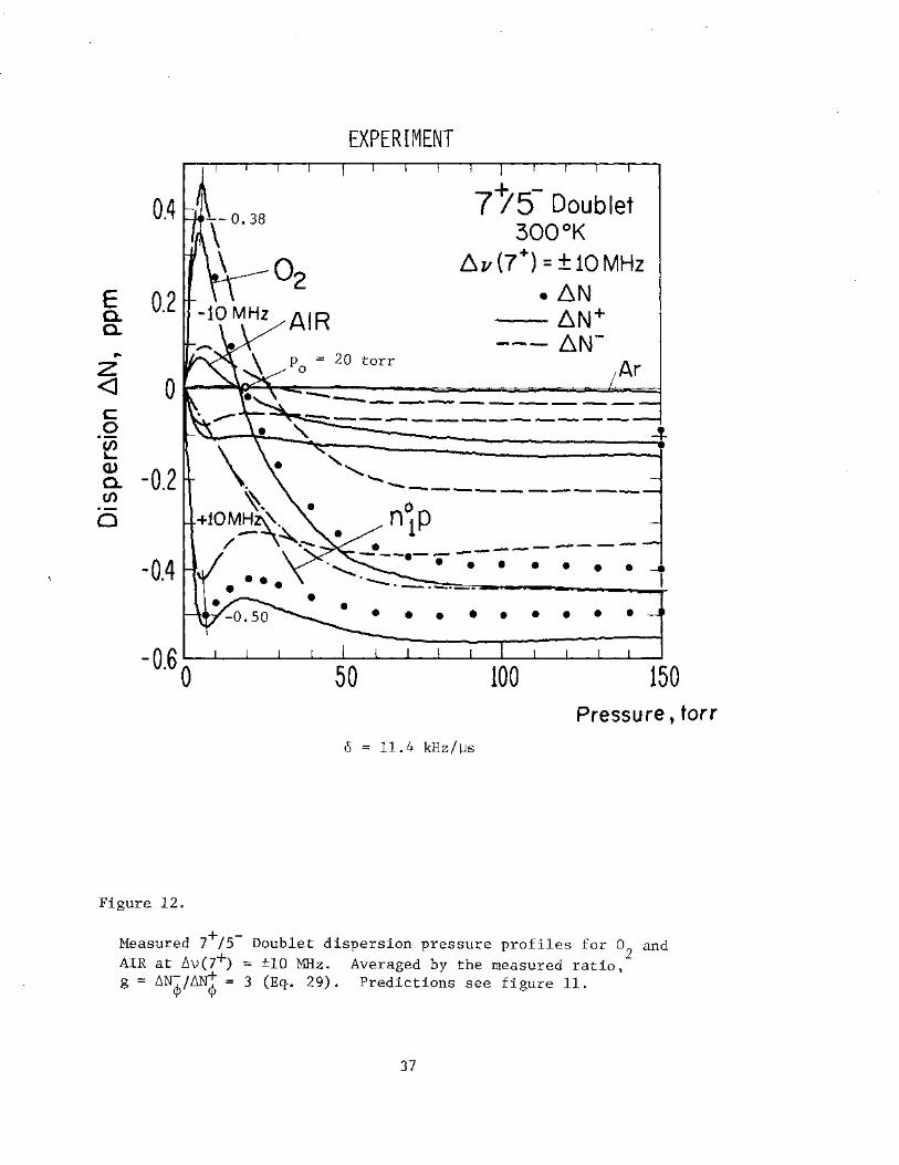
0.4
§. 0.2 0. .. z
EXPERIMENT
torr
7~5- Doublet 300°K
~v (7+) = + 10 MHz
• ~N --~N+ --- ~N-
~ o~~~~-------=~~=-~~~ c: 0 ·u; lo...
~ -0.2 CJ)
0 _...,.. ______ _
-0.4 . . . . ....... I
• • • • • •
-0.6 0 50 100 150 Pressure, torr
o = 11.4 kHz/)Js
Figure 12.
Measured 7+/5- Doublet dispersion pressure profiles for o2
and AIR at 6v(7+) = ±10 MHz. Averaged by the measured ratio, g = 6N¢/6~ = 3 (Eq.. 29). Predictions see figure 11.
37

Eaa
z
C0
a)a
0.2
E0a
z
C0U,
a,aU,
-0.2
Figure 14.+ - +
Measured dispersion profile of 3 /9 doublet at &(3 ) = —10 MHz
using the new phase meter (APPENDIX C).
Figure l. Computer plot of experi
mental 3 /9 doublt pressure profiles.
E 123 MHz; S (3 )/S (9 ) = 0.612
E
aJ-v
C0
CDCa)
Pressure, torr
38

Cmco
oII D
rO
DCD H IIH 4
S.
C 0 CD Ct
CD CD CD CD CD 0 CD CD
-o -‘ CD U,
Cl)
C -‘ CD 0 -‘
1rJ CD CD Li,
Att
enuat
ion
a,dB
/km
r)
Dis
per
sion
LN
,ppm P 0

+:--0
± N
3 13+
7+ -5
3+ 9
15~ 1
Table 5. Overview of o2-Ms Doublet Data at 300°K
Theory
\) so 0 nl 0
[GHz] -9 [Hz/torr] [10 /torr] (a) (a)
62.486 255 .9634 62.411 223 1. 2272
60.434 776 (d) 1.5626 60.306 044 1. 3487
58.466 580 • 9251 58.323 885 1.5150
56.363 393 .8539 56.264 778 .3487
(a) Table 1 - Part 2 (b) Table 2 - Part 2 (c) Equation (20) (d) See Table 10
(b)
-11.2 +10.0
- 9.40 + 9.25
+ 1.41 -12.6
--------~----
Experiment i').NL 0 0
y nl 0
[ppm] -9 [MHz/torr][lO /torr]
.43(1) 1. 82 (3) -11.2(2)
. 35 (1) 1.86(4)
.233(5) 1.92(3)
.42(1) 1. 79 (4)
---- ~----------~------------~--
so Example
[Hz/torr] (c)
1.57(5) Figs. 10-12 1. 30(7) Figs. 10,11
. 90(2) Fig. 13 1.50(8)
Fig. 14·
------ --- ----------------
2.1.3 Summary of Line Parameters (o2-o2
)
After all the complications connected with the PRS and the understanding
of its output, we can finally report some results. The quintessence of
the studies of self-pressure-broadened lines is given in Tables 5 to 7.
The actual deduced numbers indicate that dispersion profiles are suited
for quantitative work. Line parameters (y0 and 6NL) and continuum term
0
(n~) were inferred from a large number of reliable and reproducible data
points. The width y0 is the only line parameter directly measurable;
derivation of the strength S0 from 6NL requires prior knowledge of 0
y0 (Eq. 20). The uncertainties in terms of standard deviation from the
mean are small for line parameters; namely, 1 to 2 percent for y0 and
2 to 3 percent for S0• The larger uncertainties associated with 252
and 325°K results reflect a smaller body of raw data and, at 252°K,
difficulties in maintaining drift-free stable PRS operation. Data
scattering due to instrumental instabilities and S/N limitations make up
the main error sources; errors in p, T, N°, and v are at least one order
of magnitude less significant.
The conclusions to be drawn from comparison with theory for conditions
specified by (14) are enumerated as follows
1. The Lorentzian shape (Eq. 7) is valid.
2. The strength parameters S0 (300) are correct for the lines
+ + + -studied (9 , 7 , 3 , 9 , 5 ).
3. The temperature dependence of the strength, ~(9+) predicts at
252°K slightly higher values than measured (w- Eq. 32).
41

4.
5.
0 The width parameter y is proportional to pressure and decreases
with higher quantum numbers N (3+ to 9±) which is tentatively
expressed in (8).
The width y 0 (9+) varies as -0.9 T at p = const.
6. Line and continuum intensities can be separated.
7. The continuum coefficient supports the findings expressed
under 2 and 3.
8. Nonlinear overlap up to pressures of 150 torr is not detectable as
expected from the magnitude of 1° (Table 1).
9. A pressure-induced shift of the line frequency v 0
is smaller than
± 20 kHz/torr if it exists at all. Such non-existence is predicted
by theory (Dillon and Godfrey, 1972; Pickett, 1975).
10. Attenuation pressure profiles play only the role of supplementary
information due to their limited quantitative value.
We concede that line measurements are by no means completed and that for
reliable analysis of atmospheric o2-Ms transfer characteristics addi
tional lines need to be studied with particular emphasis on low tempera-
tures (180 to 260°K). One way to improve on the reliability of line
parameters is by extending the PRS frequency setting to± ~v~0.5 MHz
(e.g., Fig. 18) when the earth magnetic field, present in the laboratory,
is compensated for, thus removing Zeeman splitting (Sect. 2.3). A con-
structive approach to remaining uncertainties is to assume the validity
of the statements 1 to 9 for all lines in order to predict o2-Ms band
structure (Sect. 2.5), and then deal with the feedback from continuum
data (Sect. 2.4) to direct more work to lines, the band components.
42
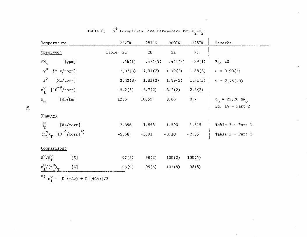
Table 6. 9+ Lorentzian Line Parameters for o2-o
2
Temperature 252°K 281°K 300°K 325°K I Remarks
Observed: Table 2c 2b 2a 2c
l!.N [ppm] .56(1) .474(3) .444(3) .39(1) I Eq. 20 0
0 [MHz/torr] 2.07(3) 1.91(2) 1. 79 (2) 1.68(3) I u = 0.90(3) y
so [Hz/torr] 2.32(8) 1. 81 (3) 1.59(3) 1.31(5) I w = 2.25(20)
0 -9 -5.2(5) -3.7(2) -3.2(2) -2.3(2) nl [10 /torr]
a [dB/km] 12.5 10.55 9.88 8.7
I a = 22.26 l!.N
0 0 0
..,.. Eq. 14 - Part 2 w
Theory:
so T [Hz/ torr] 2.396 1.855 1.590 1.315 I Table 3 - Part 1
0 -9 *) (n1)T [10 /torr] -5.58 -3.91 -3.10 -2.35 I Table 2 - Part 2
Comparison:
So/So T [%] 97 (3) 98 (2) 100(2) 100(4)
0 0 nl/(nl)T [%] 93(9) 95(5) 103(5) 98(8)
*) n~ = [K 0 (-D.v) + K0 (+D.v)]/2
N
1 3 5 7 9
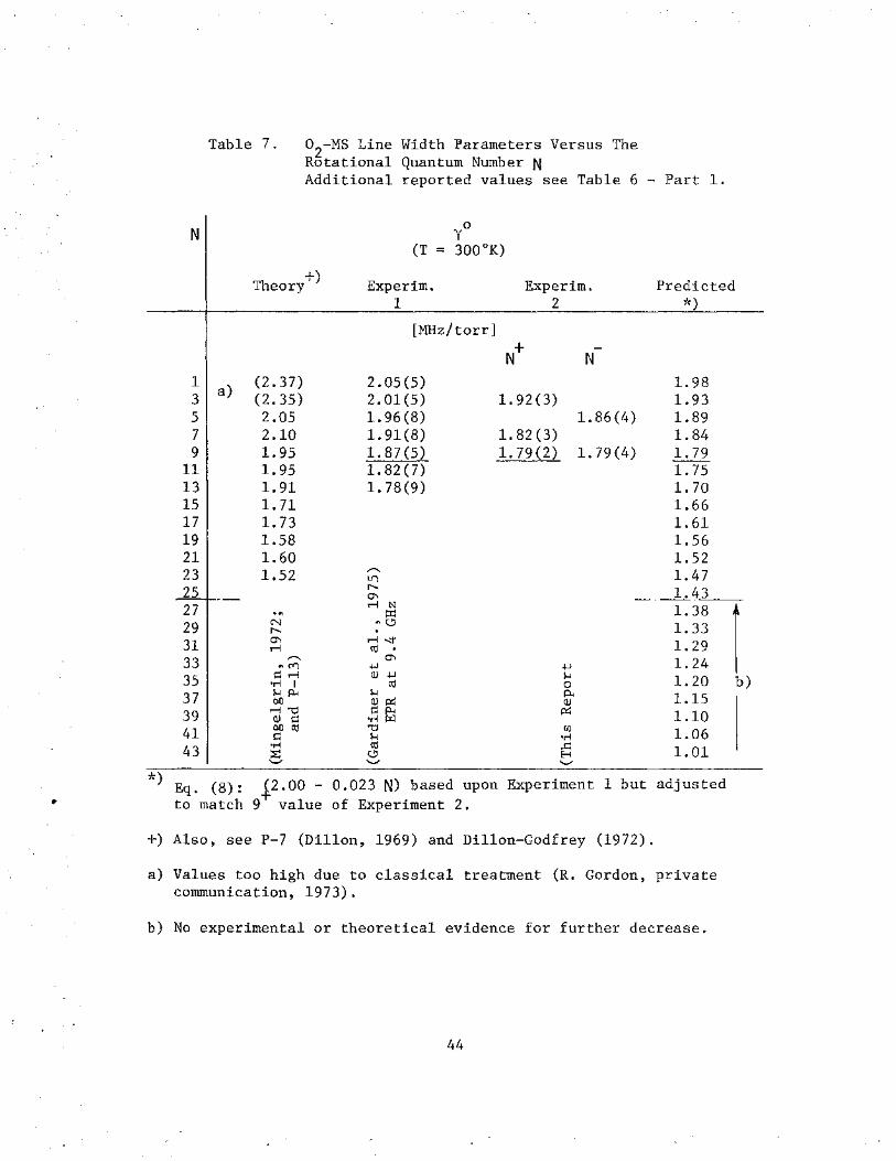
Table 7. o2-MS Line Width Parameters Versus The Rotational Quantum Number N Additional reported values see Table 6 - Part 1.
a)
.J...\ Theory''
(2.37) (2.35) 2.05 2.10 1.95 1.95 1.91 1.71 1. 73 1.58 1.60 1.52
Experim. 1
[MHz/torr]
2.05(5) 2.01(5) 1. 96 (8) 1.91(8) 1.87(5) 1. 82 (7) 1. 78(9)
Experim. 2
1.92(3)
1.82(3) 1. 79 (2)
1.86(4)
1. 79 (4)
Predicted *)
1.98 1.93 1.89 1.84 1. 79 1. 75 1. 70 1.66 1.61 1. 56 1.52 1.47
11 13 15 17 19 21 23 25 27 29 31 33 35 37 39 41 43
__ _L_~_3 __ 1. 38 1.33 1.29 1. 24 1. 20 1.15 1.10 1.06 1.01
*) Eq. (8): ~2.00- 0.023 N) based upon Experiment 1 but adjusted to match 9 value of Experiment 2.
+)Also, see P-7 (Dillon, 1969) and Dillon-Godfrey (1972).
a) Values too high due to classical treatment (R. Gordon, private communication, 1973).
b) No experimental or theoretical evidence for further decrease.
44
1 b)
2.2 Foreign Gas Pressure Broadening (AIR)
The relative concentration of atmospheric air remains constant up to
80 km height (Table 9) except for water vapor. We separate the total
atmospheric pressure into a dry and a water vapor term,
p = pd + pw ' (41)
and treat dry air (AIR) as one homogeneous gas.
Changing from oxygen, which has been treated exclusively so far, to
atmospheric air requires two adjustments in the theoretical o2
-Ms scheme
(Sect. 2.1.1- Part 2). First, all line strengths SN are reduced by
16 ~r1 = 0.2090, the product of the portion of o2 molecules and the
relative concentration of o2 in AIR; second, the pressure-broadened
widths 0 YN are modified by broadening efficiencies ~ for atmospheric
constituents other than oxygen. The atmospheric line widths, replacing
equation (8), become
*) (42)
2.?..1 Comparison of AIR-to-02
Data.
In connection with o2 dispersion and attenuation profiles, we have
repeated the same experiment with AIR on numerous occasions (e.g.,
Fig. 12). We can write for o2 that
~N (p ) = ~~kA' o m o (43)
where
kA ~ {1- A/[1 + (A!2)2]}/(l- A/2) (44)
using (26), (15), (19), (20), (23), and neglecting refractive tuning
VRN°. This approximation is valid for ±~v = 5 to 30 MHz. Since the
experimental parameter A is the same for o2
and AIR (Eqs. 23, 20, 17),
*A reduction of the nonresonant width parameter y 0 (Eq. 10) may be necessary leading to slightly different I0-value~ (Eq. 9)
45 N

the ratio of peak dispersion for AIR _and 0 2 becomes simply
Dispersion ratios for a Lorentzian line are
0 which reduces at p = canst. >> ~v/y to
and at p to
2 ~N(AIR)/~N(02 ) ~ 0.2090/md,
(45)
(47)
(48)
+ The evaluation of AIR/02
dispersion ratios in the vicinity of the 9
+ -line and 7 /5 doublet are given in Table 8. Equation (45) in particular,
determines the broadening efficience of AIR to be md = 0.94(2). For
attenuation follows
2 0 2 2 0 2 = 0.2090 md[~v + (y p) ]/[~v + (mdy p) ], (49)
which for ~v = 0 and y0p>>~v reduces to
0.2090/md (50)
A good approximation to convert o2
into AIR intensities is a multiplication
with the factor 0.225.
2.2.2 Broadening by Individual Air Components.
The indirect determination of a broadening efficiency md for AIR
using selected dispersion ratios was confirmed by direct measurements of
m for eleven air constituents. The measurements were made in two
steps. First, oxygen was admitted to generate the self-pressure-broadened
+ dispersion profiles ~N-. The second step was to stabilize the o2
+ pressure at p- and then to slowly introduce a foreign gas with increasing
m + +
total pressure p = p~ + p2 while the dispersion profiles ~Nf were
recorded (Fig. 16).
46

The broadening effect on the 9+ line was studied at 281°K for
binary mixtures of o2
with N2
, Ar, co2 , Ne, He, CH4
, Kr, N20, Xe, and
H2o vapor. The experiments were done at ±6v = 5 MHz in order to
approach isolated line behavior (K0 p ~ 0.001 ppm~O). This permits for m
data analysis the application of (Eq. 17 - Part 2)
m = pm{[(26N0
/6Nf) - 1]1
/2
- 1}/p2 • (51)
The results listed in Table 9 are based upon 6N+/6N+ ratios, although 0 f
they were found to be independent of the + or - sweep direction. The
individual broadening efficiences add up (weighted average) for a
standard dry air composition to
11 I (mr)k = md = 0.929(5),
k=l
in agreement with the value found from dispersion ratios.
(52)
The influence of water vapor on o2-MS line broadening is important
in tropospheric wave propagation. The o2-H
2o efficiency on the 9+ line
was measured to be
m = 1.25(10). w
The temperature dependencies of and
For air calculations it was assumed that
u 0.9 and v = 1
(53)
have not been studied.
(54)
Mingelgrin (1972) did "ab initio" calculations of o2-Ar line broadening
and obtained at 298°K that m(Ar) = 0.817, which compares favorably with
our result (Table 9).
Refractivity measurements on eleven atmospheric constituents were
performed at 61.2 GHz and the refractivity coefficients ~ (Eq. 2)
47
determined by a comparison with nitrogen refractivity for which
R0 = 105.6 ppm°K/torr (Newell and Baird, 1965) was assumed. The results
are included in Table 9. The weighted average
11 L (R
0r)k = R0
(AIR) = 103.49 ppm°K/torr k=l
verifies a direct refractivity measurement of AIR at 30.6 GHz.
(55)
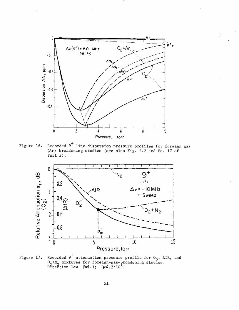
Relative attenuation pressure profiles were recorded simultaneously
with foreign gas dispersion profiles. Figure 17 depicts an example.
o2-to-AIR data (Sect. 2.1.1) and attenuation of a variable mixing ratio
02 + N2
, both can be analyzed for efficiencies md, m(N2), respectively.
The ratio at pm = 5.2 torr, for example, is a(AIR)/a(N2) = (.42/1.67)1
•1
= 0.22 yielding md = 0.95, which confirms a smaller line width in AIR
than in o2 . Analysis for m(N2
) was not attempted.
2.3 Doppler and Zeeman Line Broadening
In this section we briefly elucidate the intensity distribution of
9+, 7+, 3+, and 1+ lines in the vicinity of a line center (±~v = 0 to
1 MHz), and with the pressure below 10 torr. In the atmosphere,
the magnetic field strength H~0.3 to 1 G is omnipresent thus introduc-
ing the complications of Zeeman splitting (Sect. 2.3.3- Part 1). In the
laboratory, it is possible to compensate to H~O (Sect. 3.5.4 - Part 2)
and study the simpler case of approaching Doppler-broadening with an
unsplit line (Sect. 2.4.3- Part 1).
The H = 0 case is of experimental value in several respects: (a)
Pressure-broadening of a quasi-isolated (p = 0.5 to 10 torr) o2
-MS line
can be studied, which facilitates data analysis by avoiding the
48
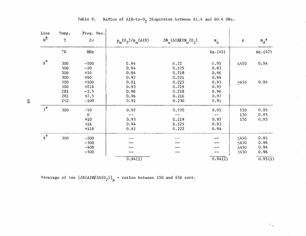
Table 8. Ratios of AIR-to-02 Dispersion between 61.4 and 60.4 GHz.
I Line Temp. Freq. Dev.
~ T !:::.v Pm(02)/pm(AIR) f:::.N (AIR)' f:::.N (02) md I p m * 0 0 d
OK MHz Eq. (45) Eq. (47)
9+ 300 -100 0.94 0.22 0.95 ~450 0.94 300 -10 0.94 0.225 0.93 300 +10 0.94 0.218 0.96 300 +50 0.92 0.221 0.94 300 +100 0.91 0.225 0.93 I ..(450 0.94 300 +216 0.93 0.219 0.95 281 -3.5 0.96 0.218 0.96 281 +7.5 0.96 0.216 0.97
~ 252 -100 0.92 0.230 0.91 \0
-7+ 300 -10 0.92 0.220 0.95 150 0.95
0 -- -- -- 150 0.95 +10 0.93 0.219 0.95 150 0.95 +16 0.94 0.225 0.93 +116 0.92 0.222 0.94
9+ 300 -200 -- -- -- ..;S_450 0.95 -300 -- -- -- ..;S_450 0.96 -400 -- -- -- ..;S_450 0.94 -500 -- -- -- ~450 0.96
0.94(2) 0.94(2) 0.95(1)
*Average of ten [!:::.N(AIRY!:::.N(02)Jp- ratios between 150 and 450 torr.

k
1
2
3
4
5
6
7
8
9
10
11
Table 9. Broadening Efficiency m(9+) and Refractivity N° Measured at \J = 61 156 MHz, T = 281 °K, p ~ 20 torr, for Different Air Components, and the Relative Concentration r of Dry Air Components.
Component r N°(281)
ppm by vol
ppm/torr ppm°K/torr
Oxygen
Nitrogen
Argon
Carbon Dioxide
Neon
Helium
Methane
Krypton
Hydrogen
Ar
Ne
He
Kr
Nitrous Oxide N20
Xenon Xe
Dry Air AIR
209 460 0.3405 (±60)
780 840 0.3758
9 340 0.3549
320t 0.6335
18.18 0.08659
5.24 0.0450
1.2-2t 0.5672
1.14 0.5428
o.5t
o.5t o. 7138
0.087 0.8636
106 0.3696
Water Vapor H2o variable 6.666
95.67(a)
105.60*
99.73
178.0
24.33
12.65
159.4
152.5
48.9
200.6
242.7
1
0.911(5)
0.805(5)+)
0.89(1)
0.61(1)
0.70(1)
1.03(1)
0.68(1)
0.88(1)
0.63(1)
(b) 11 103.5 E(rm)=0.929(5)
fct(T) (Eq. 2)
k=l
1. 25(10)
* 0 0 Reference value; all measured R are relative to the R (N2 ) - value given by Newell and Baird (1965).
+) m(Ar) = 0.817, calculated by Mingelgrin (P-13).
t Average value (a) - See Table 13
(b) Measured at \J/2 = 30.6 GHz
50
z <l c
-0.1
~~~(g+) = 5.0 MHz 281 °K
·* -0.3 .... Q) a. (/)
0 -0.4
Figure 16.
en "0
~
e:s c 0 --0 N
~0 a>---<( Q)
> -0 Q)
a::
0 2 4 6 8 10 Pressure, torr
Recorded 9+ line dispersion pressure profiles for foreign (Ar) broadening studies (see also Fig. 2.2 and Eq. 17 of Part 2).
0
1 b.v =- 10 MHz +Sweep
2
3 0 5 10 15 Pressure, torr
Figure 17. Recorded 9+ attenuation pressure profile for o2
, AIR, and o
2+N2 mixtures for foreign-gas-broadening stud1es.
Detection law S~.l; ~.2•105.
51
gas

•
continuum; (b) the transition frequency \) 0
can be determined more
accurately from ~N(p+O) = 0; (c) the relative maximum line attenuation a 0
(Fig. 22) at ~V = 0 is well defined; and (d) the resolving power of
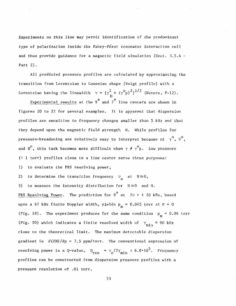
the PRS can be evaluated. + Figure 18 illustrates such a case for the 9
line. The Doppler width is The rates for maximum
attenuation and dispersion to approach zero are 0.68 and 0.61 times
0 S p/yD, respectively, when p < 0.01 torr. Pure pressure-broadening
(Sect. 2.1) exists for all ~v when p > 0.5 torr.
The anomalous Zeeman effect splits the line N into
3(2N±l) components that are spread as a function of H over a 1 to
2 MHz wide band to either side of the line center V Each Zeeman 0
component undergoes the gradual transition from pressure to Doppler
broadening. By a judicious choice of the orientation between H and
the magnetic field vector ~ of radiation, assumed linearly polarized,
+ one can selectively excite two types (a- and n) of Zeeman transitions.
+ + For example, the 9 line splits into 19TI (H II~) or 38a- (Hl '!¥ components.
Figures 19 and 23 depict pressure profiles for TI and a-types of the
9+ and 3+ lines under the field strength (0.53 G) present in the laboratory.
Pure pressure-broadening (Sect. 2.1) exists for ±~v~2 MHz and p > 4 torr •
Individual Zeeman components are not resolved.
+ The normal Zeeman effect of the 1- lines has the simplest splitting
pattern, either two a or one TI component whereby only the a
components shift away from the line center. Figure 24 gives examples of
predicted pressure profiles for the 1+ line. For the a-type split we
note a resolution of the two components on the 0 to 1 torr pressure scale.
52
Experiments on this line may permit identification of the predominant
type of polarization inside the Fabry-Perot resonator interaction cell
and thus provide guidance for a magnetic field simulation (Sect. 3.5.4 -
Part 2).
All predicted pressure profiles are calculated by approximating the
transition from Lorentzian to Gaussian shape (Voigt profile) with a
Lorentzian having the linewidth 2 0 2 1/2 y = [y + (y p) ] (Waters, P-12). D
Experimental results at the 9+ and 7+ line centers are shown in
figures 20 to 22 for several examples. It is apparent that dispersion
profiles are sensitive to frequency changes smaller than 5 kHz and that
they depend upon the magnetic field strength H. While profiles for
pressure-broadening are relatively easy to interpret because of y0, S0
,
and N°, this task becomes more difficult when y I y0 p. Low pressure
(< 1 torr) profiles close to a line center serve three purposes:
1) to evaluate the PRS resolving power,
2) to determine the transition frequency \) 0
at H~O,
3) to measure the intensity distribution for H~O and H.
PRS Resolving Power. The prediction for 9+ at ~V = ± 20 kHz, based
upon a 67 kHz finite Doppler width, yields p = 0.045 torr at H = 0 m
(Fig. 18). The experiment produces for the same condition p = 0.06 torr m
(Fig. 20) which indicates a finite resolved width of Y ,;, 90 kHz min
close to the theoretical limit. The maximum detectable dispersion
gradient is d(~N)/dp = 7.5 ppm/torr. The conventional expression of
resolving power is a Q-value, Q res v /2y . = 6.8•105 . Frequency o m1n
profiles can be constructed from dispersion pressure profiles with a
pressure resolution of .01 torr.
53

Table 10. 9+ and 7+.Line Center Frequencies
9+ Line (Fig. 19), H ,;, 0
T \) ~ IF 0
OK MHz MHz MHz
252 61 150.583(5) 15.056 414(1) 40. 883 845
281 .575(5) 412(1) 783
300 .565(5) 410(1) 830
325 .559(5) 408(1) 855
~ 2028
Exp. .570(10)
Th. .567 Table 2 - Part 1
7+ Line H = 0.53 G
300 60 434.782(5) 15.009 065(1) -40.883 822
~= 2016
Exp. • 776 (10)
Th. .778 Table 2 - Part 1
Transition Frequency. The frequency v is defined by assuming for 0
H ,;, 0 that ~N = 0 for p ,;, 0 to 0.1 torr. This is not exactly true
since at ~V(9+) = 0, first the refractive tuning (-19 kHz/torr) produces
a small positive dispersion ~NL until next the negative continuum
0 takes over. For example, 9+, 02, 300°K, H = 0 yields: nlp
p, torr _3 0 0.5 1 2 3 3.5
~N, ppm•lO 0 8.0 (Max) 6.5 3.0 0.3 -1.0
On the other hand, the speed o = ± 16 kHz/~s forces a shift upon
54

\J1 \J1
Table 11. Measured Peak Dispersion ~N , Pressure p , and Width y0 Around the 9+ Line Center o o m
(~v = ± 5 MHz, T = 281 K, Oxygen, H = 0.53 gauss, +Sweep).
~N+ I D p+ ~v/p+
l~vl 0
Mean 1
Differ. m m
- + - t Mean - t Mean
[MHz] [ppm] I [torr] [MHz/torr]
0.10 .343 -.400 .372 I
-.057 .08 .10 .09 1. 25 1.00 1.13 0.25 .410 -.435 .423
I -.025 .18 .20 .19 1. 39 1. 25 1. 32
I 0.50 .426 -.450 .438
I -.025 .28 .32 .30 1. 79 1.56 1.68 1 .434 -.479 .457 I -.045 .53 .61 .57 1.89 1.64 1.77 2 .441 -.490 .466 I -.049 1. 06 1.12 1. 09 1.89 1. 79 1.84 2.5 .442 -.495 .468 I -.053 1. 31 1.42 1. 37 1. 91 1. 76 1.84 3.5 .441 -.499 .470 I -.058 1. 81 1. 97 1.89 1.93 1. 78 1.85 5 .441 -.503 .472 I -.062 2.54 2. 72 2.63 1.97 1.84 1.90
5-30 Table 2b: .474(3) 1. 91 (2) ------ ------ , __ -----------
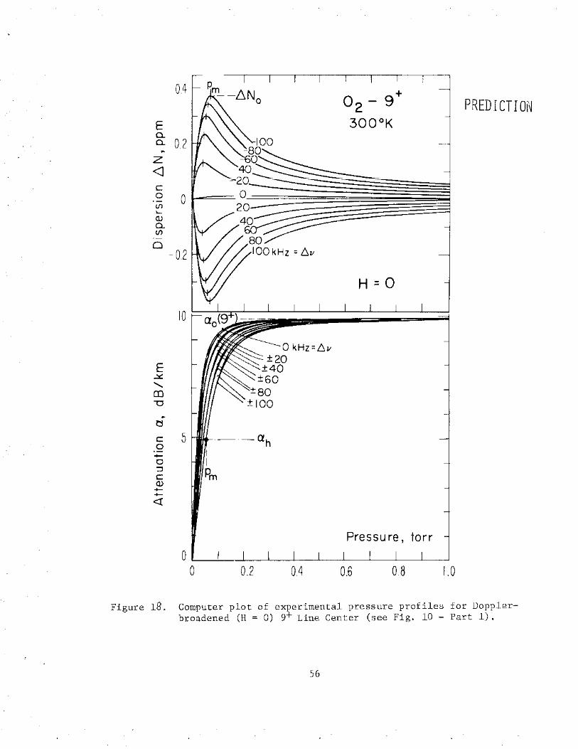
0.4 -~N 0 - 9+ 0 PREDICTION 2
E 300°K a.
.. a. 0.2 z <1 c 0 0 (/) ~
Q) a. (/)
0 -0.2
H=O
10
OkHz=6v
E ±20
±40 .::st:. ±60 ......... CD 80 "'C ±100 .. ~
c 5 .Q -0 I :::I Pm c Q) --<(
Pressure, torr
0 0 0.2 OA 0.6 0.8 1.0
Figure 18. Computer plot of experimental pressure profiles broadened (H = 0) 9+ Line Center (see Fig. 10 -
for Doppler-Part 1).
56

04
E 0.2 0.. 0..
z <J c 0 (./) lo... Q)
0.. (./)
0 -0.2
10
E ..:::t:. ......... CD "0
~
t:!
c 5 0 -0 ::::l c Q) +-..... <(
Figure 19.
1T -Components ( 19)
5 ·-a h
02 - g+
3QQ°K
H = 0.53 gauss
1 MHz = D.v
o-±- Components (38)
Pressure, torr 10
Computer plot of experimental pressure profiles for Dopplerand Zeeman-broadened 9+ Line Center.
57
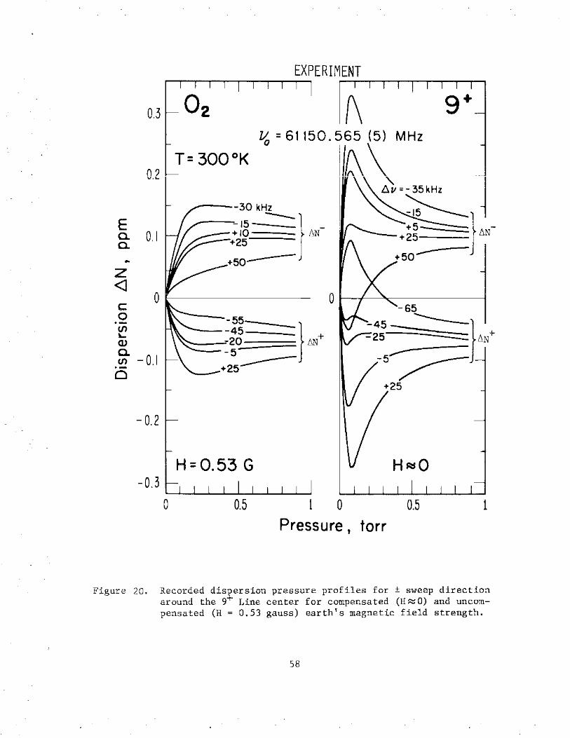
EXPERIMENT
0.3 {\ g+
fl? v.t..
E c. c. 0.1
.. z <J
0 0 c -65 0
~~- -} ---} (/) \... -20 liN+ liN+ Q) c.
-0.1 -5 -5/--(/) +25-----
0
-0.2
-0.3
0 0.5 1 0 0.5 1
Pressure , torr
Figure 20. Recorded dis~ersion pressure profiles for ± sweep direction around the 9 Line center for compensated (H~O) and uncompensated (H = 0.53 gauss) earth's magnetic field strength.
58
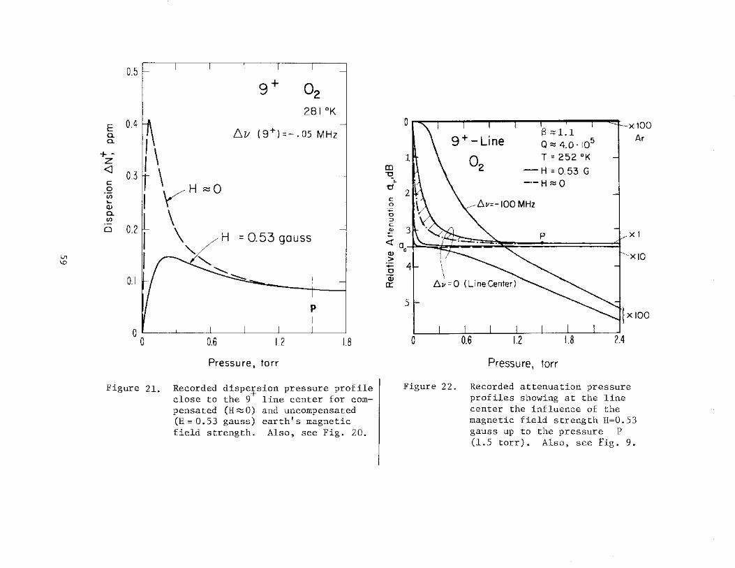
Ul 1.0
0.5
E 0.4 ~ a. a. +~ z <I 0.3 c:
.Q II) ..... Q)
a. II)
0 0.2 ..
I~
0.1
00
. '\..../
0.6
g+ 02 281 °K
D.v ( g+) =-. os MHz
H = 0.53 gauss
1.2
p I
Pressure, torr
1.8
Figure 21. Recorded dispe+sion pressure profile close to the 9 line center for compensated (H ~ 0) and uncompensated (H=0.53 gauss) earth's magnetic field strength. Also, see Fig. 20.
0 x100 Ar
t.~ ~ 4.0 · ro- I 02 T = 252 °K
CD l\ \ -H = 0.53 G -q ... -·-H~o d
2 c 0
:;:: 0 :J c
~ 3(\ -........:~ ""-... p l~x I <:(a Q) 0 > I I;---......_ ............ r--xro
:;::: 0
Q) a::
5
0 2.4
Pressure, torr
Figure 22. Recorded attenuation pressure profiles showing at the line center the influence of the magnetic field strength H=0.53 gauss up to the pressure P (1.5 torr). Also, see fig. 9.

vR(o=O) with the difference lvR(+o) ·- vr(-o) I = 28(4) kHz, which is
sufficient to produce close to a line center vastly different dispersion
profiles (Fig. 20). The center V was determined when the setting 0
~V(9+) = ± 14 kHz produced ~N- + ~N+ ~ 0 for p = 0 to 0.1 torr.
The results are listed in Table 10 and there was no difference for
H = 0 and H = 0.53 G. The very slight systematic temperature dependence
of V indicates that the above procedure was somewhat erroneous although 0
not more than other reported values. The line contributions +~N~( +14kHz)
+ -~N1 (- 14kHz) probably did not cancel completely because of
g ~ 1 (Eq. 29, Fig. 7).
Intensity Distribution. The ~N(p)-profiles have the potential for
absolute intensity measurements. A puzzling problem is whether or not
overlap interference exists between Zeeman components in analogy to the
pressure-broadened o2-Ms band shape. That question surfaced when
Waters (1973) measured emission from well-resolved (y~3 MHz, h > 40 km)
02-MS lines originating in the upper stratosphere. On the edges of the
band, thermal emission from high N-number lines penetrates the lower
atmosphere. Against the continuum background, a peak emission
line centers was measured toward zenith to be (Waters, 1973)
- - -N-number 31 29 27 25 -~-·-······· ··~·~--.. ~-----~----------
Measured T o' OK 6.5 10 13 11 22 40
Calculated T o' OK 2.8 5 7.8 7
Observation height h, km 0 0 0 0 3.3 4.9
T 0
95
11.8
at the
-23
5
2.4
0
which is consistently higher when compared with calculations based upon
Lenoir's (1968) formulation. Another plausible explanation for the
60
,
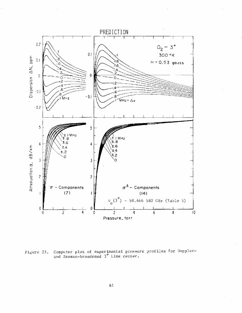
0.2
E a. 0.1 a. ~
z <J c 0 (/) ..... (])
0
~ -0.1 0
-0.2
5
E 4
..:.: ........ en "0
3 ~ c 0 - 2 0 ::J c (])
-<{
0 0
Figure 23.
5
4
3
2
7r- Components (7)
2 4
PREDICTION
0 - 3+ 2
300 °K
H = 0.53 gauss
+ (J"-- Components
(14)
\) (3+) 0
58.466 580 GHz (Table 5)
2 4 6 8 Pressure, torr
10
Computer plot of experimental pressure profiles for Dopplerand Zeeman-broadened 3+ Line center.
61

(a) PREDICTION o.oe
0.06
[ 0.04 0.
0.02 z <I 12.6·10-3
0 0 0 ppm/torr ·r-i Ul !-1 QJ -0.02 0. Ul
·r-i 0
-0.04
-0.06
0 0.2 0.4 o.e o.e 1.0
1.6
] 02 - 1+
- 300°K ~ 1.2 '"d
MHz (j
0 0.8 0
•r-i .w ctl ::l 0 QJ .w 0.4 .w <t: ±
0 - Components
H = 0.53 gauss
0
I I I 0 o.z 0.4 o.e o.e 1.0
Pressure torr
62
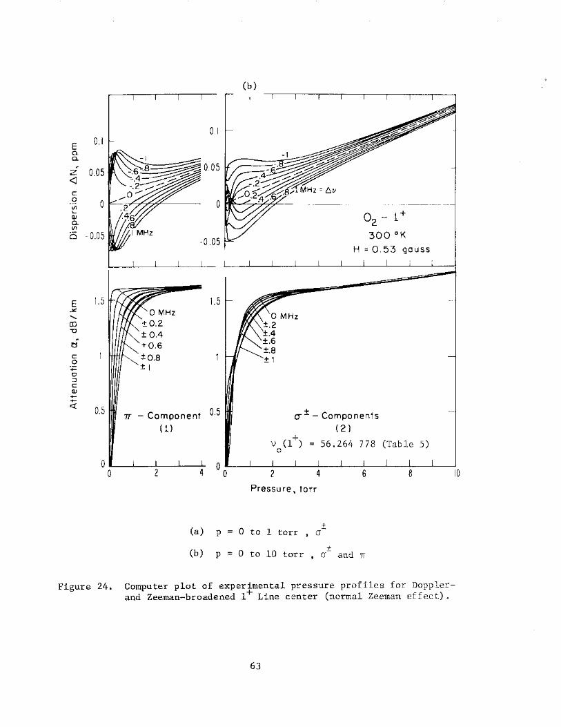
E 0.1 a. a.
z 0.05 <J c .9 0 Vl .... Q)
a. Vl
0 -0.05
E 1.5 .:t! ...... 0) '0
~
~
c 0 +-0 ::I c Q) +-..... <t 0.5
0 0
Figure 24.
7T
1.5
+0.6 ±o.a ±I
-Component 0.5
(1)
(a) p
(b)
02- t+
300 °K
H = 0.53 gauss
0 MHz ±.2 ±.4 ±.6 ±.8 ±1
+ a--- Components ( 2)
\) (1+) = 56.264 0
2 4
Pressure, torr
+ 0 to 1 torr , a-
+
778 (Table 5)
6 8
(b) p = 0 to 10 torr , a- and TI
10
Computer plot of experimental pressure profiles for Dopplerand Zeeman-broadened 1+ Line center (normal Zeeman effect).
63
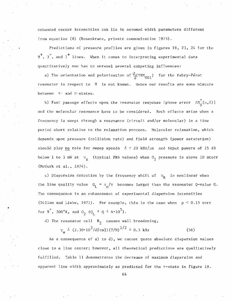
enhanced center intensities can lie in assumed width parameters different
from equation (8) (Rosenkranz, private communication 1975).
Predictions of pressure profiles are given in figures 19, 23, 24 for the
+ + + 9 , 3 , and 1 lines. When it comes to interpreting experimental data
quantitatively one has to unravel several competing influences:
a) The orientation and polarization of~(TEM001 ) for the Fabry-Perot
resonator in respect to H is not known. Hence our results are some mixture
between TI- and a-states.
+ b) Fast passage effects upon the resonator response [phase error 6N¢(a,o)]
and the molecular resonance have to be considered. Both effects arise when a
frequency is swept through a resonance (circuit and/or molecular) in a time
period short relative to the relaxation process. Molecular relaxation, which
depends upon pressure (collision rate) and field strength (power saturation)
should play no role for sweep speeds o < 20 kHz/~s and input powers of 15 dB
below 1 to 3 mW at VR (typical PRS values) when o2 pressure is above 10 mtorr
(McGurk et al., 1974).
c) Dispersion detection by the frequency shift of VR is nonlinear when
the line quality value QL = v0/y becomes larger than the resonator Q-value Q.
The consequence is an enhancement of experimental dispersion intensities
(Dillon and Liebe, 1971). For example, this is the case when p < 0.15 torr
for 9+, 300°K, and o2 (QL ~ Q ~ 4•105).
d) The resonator cell R2 causes wall broadening,
y ~ (2.30•103/d[cm])(T/M) 112 ~ 0.5 kHz w
(56)
As a consequence of a) to d), we cannot quote absolute dispersion values
close to a line center; however, all theoretical predictions are qualitatively
fulfilled. Table 11 demonstrates the decrease of maximum dispersion and
apparent line width approximately as predicted for the TI-state in figure 19.
64
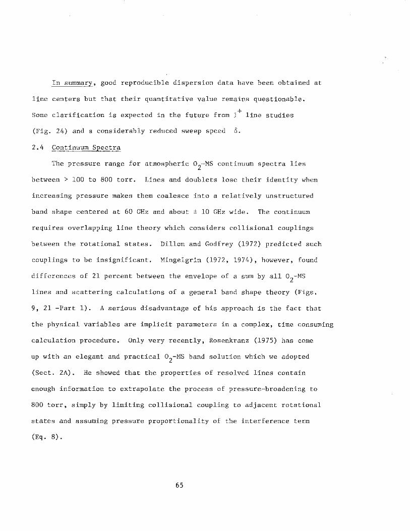
In summary, good reproducible dispersion data have been obtained at
line centers but that their quantitative value remains questionable.
Some clarification is expected in the future from 1+ line studies
(Fig. 24) and a considerably reduced sweep speed o.
2.4 Continuum Spectra
The pressure range for atmospheric o2-Ms continuum spectra lies
between > 100 to 800 torr. Lines and doublets lose their identity when
increasing pressure makes them coalesce into a relatively unstructured
band shape centered at 60 GHz and about ± 10 GHz wide. The continuum
requires overlapping line theory which considers collisional couplings
between the rotational states. Dillon and Godfrey (1972) predicted such
couplings to be insignificant. Mingelgrin (1972, 1974), however, found
differences of 21 percent between the envelope of a sum by all o2
-Ms
lines and scattering calculations of a general band shape theory (Figs.
9, 21 -Part 1). A serious disadvantage of his approach is the fact that
the physical variables are implicit parameters in a complex, time consuming
calculation procedure. Only very recently, Rosenkranz (1975) has come
up with an elegant and practical o2-Ms band solution which we adopted
(Sect. 2A). He showed that the properties of resolved lines contain
enough information to extrapolate the process of pressure-broadening to
800 torr, simply by limiting collisional coupling to adjacent rotational
states and assuming pressure proportionality of the interference term
(Eq. 8).
65
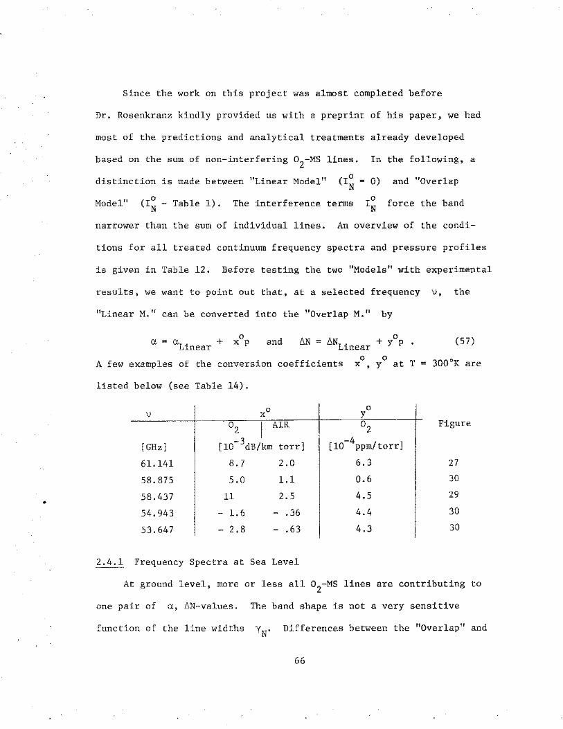
•
Since the work on this project was almost completed before
Dr. Rosenkranz kindly provided us with a preprint of his paper, we had
most of the predictions and analytical treatments already developed
based on the sum of non-interfering 0 -MS 2 lines. In the following, a
distinction is made between "Linear Model" (Io N 0) and "Overlap
Model" (Io -N Table 1). The interference terms Io
N force the band
narrower than the sum of individual lines. An overview of the condi-
tions for all treated continuum frequency spectra and pressure profiles
is given in Table 12. Before testing the two "Models" with experimental
results, we want to point out that, at a selected frequency v, the
"Linear M." can be converted into the "Overlap M." by
a= a + Linear 0
X p and 0 ~N = ~NLinear + y p (57)
A few examples of the conversion coefficients 0 0
x , y at T = 300°K are
listed below (see Table 14).
0 \) X
02 I AIR
[l0-3dB/km torr] [GHz]
61.141 8.7 2.0
58.875 5.0 1.1
58.437 11 2.5
54.943 - 1.6 - .36
53.647 - 2.8 - .63
2.4.1 Frequency Spectra at Sea Level
0 y 02
-4 [10 ppm/torr)
6.3
0.6
4.5
4.4
4.3
Figure
27
30
29
30
30
At ground level, more or less all o2-Ms lines are contributing to
one pair of a, ~N-values. The band shape is not a very sensitive
function of the line widths yN. Differences between the "Overlap" and
66
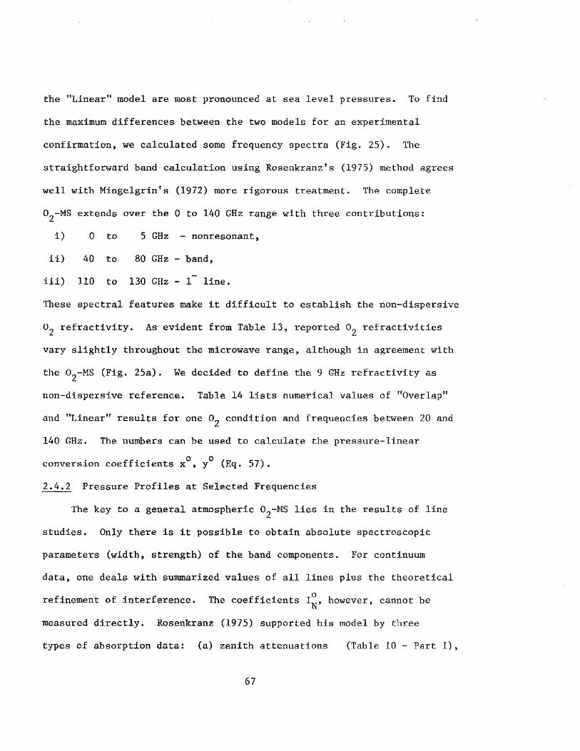
the "Linear" model are most pronounced at sea level pressures. To find
the maximum differences between the two models for an experimental
confirmation, we calculated some frequency spectra (Fig. 25). The
straightforward band calculation using Rosenkranz's (1975) method agrees
well with Mingelgrin's (1972) more rigorous treatment. The complete
02-MS extends over the 0 to 140 GHz range with three contributions:
i) 0 to 5 GHz - nonresonant,
ii) 40 .to 80 GHz - band,
iii) 110 to 130 GHz - 1- line.
These spectral features make it difficult to establish the non-dispersive
o2 refractivity. As evident from Table 13, reported o2 refractivities
vary slightly throughout the microwave range, although in agreement with
the o2-Ms (Fig. 25a). We decided to define the 9 GHz refractivity as
non-dispersive reference. Table 14 lists numerical values of "Overlap"
and "Linear" results for one o2 condition and frequencies between 20 and
140 GHz. The numbers can be used to calculate the pressure-linear
conversion coefficients x0, y0 (Eq. 57).
2.4.2 Pressure Profiles at Selected Frequencies
The key to a general atmospheric o2
-Ms lies in the results of line
studies. Only there is it possible to obtain absolute spectroscopic
parameters (width, strength) of the band components. For continuum
data, one deals with summarized values of all lines plus the theoretical
refinement of interference. 0 The coefficients IN, however, cannot be
measured directly. Rosenkranz (1975) supported his model by three
types of absorption data: (a) zenith attenuations (Table 10- Part 1),
67

(b) satellite (NIMBUS 5) measurements of atmospheric brightness temperature
TH at 54.9 GHz (Eqs. 58, 59), and (c) laboratory attenuation measurements
by Poon (1974) at 58.82 GHz (02 , 295°K, 0-320 torr). Direct measurements
of a and ~N between 100 and 800 torr are the most sensitive test.
The discrepancies Overlap-to-Linear are, for example (Table 14), for 0 0 k
attenuation -40, 0, +18, 0, -80% at 50, 55.4, 60, 63.6, 100 GHz, respectively;
and for o2 dispersion 2.5, 26, 82, 38, 2.5% at 50, 57, 60, 62, 70 GHz,
respectively. A main objective of this project was the confirmation of
o2-Ms theory at frequencies selected by NASA and NOAA for temperature
soundings. Figure 29 illustrates the differences Overlap-to-Linear for
the three NIMBUS 5 o2-Ms channels (Sabatini, 1972).
Measurements of dispersion and relative attenuation pressure profiles
have been conducted, so far, under the following conditions:
V, GHz p, torr T, OK Example
61.15{~~:; 0 - 450 (760) 300, 282, 252 Fig. 26, 27
60.4 {~:~1 0 - 450 300 Fig. 28
58.87 0 - 150 300 Fig. 30
58.4 0 - 800 300 Fig. 29
Dispersion measurements are sensitive to better than ± 0.005 ppm
and the accuracy depends upon the assessment of the phase error ~N¢.
The phase error ratio g found from line studies (Fig. 7) was extra-
polated, but there was no way to check if g remained constant up to
800 torr. This uncertainty has been considerably reduced by the new
phase meter. Averaged dispersion results (Eq. 29) are compared with
either PREDICTIONS, N(VR)- N(VR/2), or THEORY, ~N(v). In the case of THEORY,
68

0\ \0
Figure Table
25a 25b
T 13 T 12
33 34 31c 32 31c 3lc 30
T 15 32 31b 30
T 16 31b 31b 3la 29 31a 32 30 31a 30
T 17 28 27 26
\) /':.,_\)
[GHz) 0 - 140
20 - 140 20 - 140
0 - 72 40 - 140 40 - 140
50.300 0±0.1 52.800 0±0.1 52.800 0±0.1 53.647 0±0.1 53.647 0 53.647 0 54.900 0±0.1 54.943 0±0.1 54.943 0 54.943 0 54.960 0±0.1 55.500 0±0.1 57.950 0±0.1 58.437 0 58.800 0±0.1 58.800 0±0.1 58.865 0 58.875 0±0.1 58.875 0 58.875 0 60.435 0±0.3 61.141 0 61.151 0±0.3
Table 12. Overview of Treated o2-Ms Continuum Data
p T 02 AlB a 6N Theory Experiment Linear Overlap Predict. Measure d
[torr] [OK] 760 300 X X X X X
760 300 X X X X X
760 300 X X X
X X X
760,570,380,190 200, 300 X
760,570,380,190 200, 300 X
0 - 800 250- 300 X X X X
0 - 800 300 X X X X
0 - 800 250- 300 X X X X
0 - 800 200- 300 X X X X
0 - 800 300 X X X X X X
0 - 400 200- 300 X X X
0 - 800 300 X X X X
0 - 400 200- 300 X X X X
0 - 400 300 X X X X X X
0 - 200 200- 300 X X X
0 - 800 250- 300 X X X X
0 - 800 250- 300 X X X X
0 - 800 250- 300 X X X X
0 - 800 300 X X X X X X X
0 - 800 250- 300 X X X X
0 - 800 300 X X X X
0 - 200 300 X X X X X X X
0 - 200 200- 300 X X X X
0 - 200 300 X X X X X X
0 - 100 200- 300 X X X
0 - 1000 300 X X X X X
0 - 800 300 X X X X X X X
0 - 1000 300 X X X X X
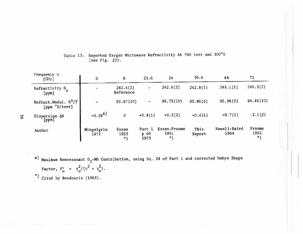
Table 13. Reported Oxygen Microwave Refractivity At 760 torr and 300°K
(see Fig. 25).
Frequency[GHz] 0 9 23.6 24 30.6 48 72
Refractivity N 242.4(2) - 242.6(2) 242.8(1) 243.1(1) 240.3(2)
[ppm] Reference
Refract.Modul. R°/T 95.67(10) - 95.75(10) 95.86(5) 95.96(5) 94.85(10)
[ppm °K/torr]
Dispersion039a)
0 +0.4(1) +0.2(2) +0.4(1) +0.7(1) -2.1(2)[ppm]
Author Mingeigrin Essen Part 1 Essen-Froome This Newell-Baird Froome
1972 1953 p 60 1951 Report 1964 1955*) 1973 *) *)
a)Maximum Nonresonant 02-MS Contribution, using Eq. 24 of Part 1 and corrected Debye Shape
*
Factor, F’= y2/(\)2 +
Cited by Boudouris (1963).
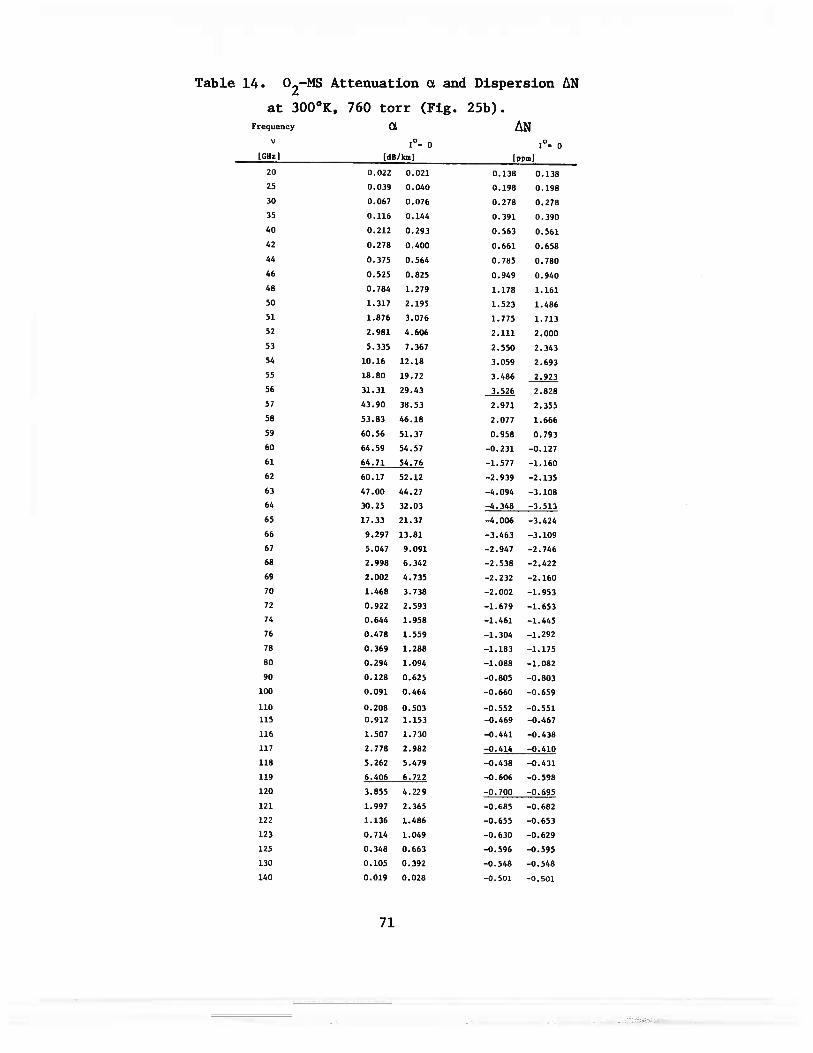
Table 14. 02—MS Attenuation a. and Dispersion AN
at 300°K, 760 torr (Fig. 25b).Frequency a.
V 10=0 10=0
[CHe] [dB/kml [ppm]
20 0.022 0.021 0.138 0.138
25 0.039 0.040 0.198 0.198
30 0.067 0.076 0.278 0.278
35 0.116 0.144 0.391 0.390
40 0.212 0.293 0.563 0.561
42 0.278 0.400 0.661 0.658
64 0.375 0.564 0.785 0.780
66 0.525 0.825 0.949 0.940
48 0.784 1.279 1.178 1.161
50 1.317 2.195 1.523 1.486
51 1.876 3.076 1.775 1.713
52 2.981 4.606 2.111 2.000
53 5.335 7.367 2.550 2.343
54 10.16 12.18 3.059 2.693
55 18.80 19.72 3.486 2.923
56 31.31 29.43 3.526 2.828
57 43.90 38.53 2.971 2.355
58 53.83 46.18 2.077 1.666
59 60.56 51.37 0.958 0.793
60 64.59 56.57 —0.231 —0.127
61 64.71 54.76 —1.577 —1.160
62 60.17 52.12 —2.939 —2.135
63 47.00 44.27 —4.094 —3.108
64 30.25 32.03 —4.348 —3.513
65 17.33 21.37 —4.006 —3.424
66 9.297 13.81 —3.463 —3.109
67 5.047 9.091 —2.947 —2.746
68 2.998 6.342 —2.538 —2.422
69 2.002 4.735 —2.232 —2.160
70 1.468 3.738 —2.002 —1.953
72 0.922 2.593 —1.679 —1.653
74 0.644 1.958 —1.461 —1.445
76 0.478 1.559 —1.304 —1.292
78 0.369 1.288 —1.183 —1.175
80 0.294 1.094 —1.088 —1.082
90 0.128 0.625 —0.805 —0.803
100 0.091 0.464 —0.660 —0.659
110 0.208 0.503 —0.552 —0.551
115 0.912 1.153 —0.469 —0.467
116 1.507 1.730 —0.441 —0.438
117 2.778 2.982 —0.414 —0.410
118 5.262 5.479 —0.438 —0.431
119 6.406 6.722 —0.606 —0.598
120 3.855 4.229 —0.700 —0.695
121 1.997 2.365 —0.685 —0.682
122 1.136 1.486 —0.655 —0.653
123 0.714 1.049 —0.630 —0.629
125 0.348 0.663 —0.596 —0.595
130 0.105 0.392 —0.568 —0.548
140 0.019 0.028 —0.501 -0.501
71

-.....! N
0 2-MS 4 [ 760 torr
300 °K
l 1~-~---
21-
I
E 0.. 0..
I I I I I 1.------T-- . T ...... I
LINEAR vs I ~~ INGELGRI N THEORY~-
--Linear Overlap Calcul.
J6Nmaxl= 6.41 ppm
-·- Scattering Calculation J6Nmaxl = 7.77
':1 60 t- !:·
50
~ 40 ' (l) "0
-Linear Overlap Calcu lotion a:max = 56.4 dB/km
-·-Scattering Calculation a max = 68.4
z 0 <J a
c 0
~ -1 Q) 0.. rn 0
-2.- X rU s
I I I I I I I - .
c 30 .~ -0 ::J c ~ ;r 20
-f.:l::;:::;:;:;j-l\-- 0.5 a max
6Nmax
---1::::::::::::::1..-1- Measurement
-l~ l ______ -4
-I I I I I I
1 L1ne-
or
Range
ao ( n = 6.41--
10
01 I L..:-"'1 II I :=t I 1,......, 1'- I I 0 20
Figure 25a.
40 60 80 Frequency, G Hz
100 120 140 20 40 60 80 100 120 140
F.equency, GHz
The o2 Microwave Spectrum of dispersion 6N and attenuation a between 0 and 140 GHz and tfie frequency range of the measurements. The experimental dispersion 6N is measured as difference in refractivity at v and v/2. x I : Reported o
2 refractivities - see Table 13.
Scattering calculations by Mingelgrin (1972, 1974, and Fig. 9- Part 1).

-....J LV
4
.3
E z. a. a.
z <l c .2 !J) ..... Q> a. !J)
0
-I
0 -2.
-3
-4
-5
20 40 so eo 100
Frequency v, GHz
LINEAR VS. ROSENKRANZ THEORY
r-
60 1-
E .:X: 1-....... co " ~ 40 ..._ ~
c 0 - 1-0 ::I c Q> ::: 20 ..._ <(
I I I I I I I I T I
{\
r. I\: I .
I I I 'I ,, ,,
'
0 2-MS 760 torr 300 °K
-
-
-
-
-
0 t j_~:----w A j r-
I l L __ _l________l_ I I I I 120 140 20 40 60 so 100 120 140
Frequency v, GHz
Figure 25b. The o2-MS microwave spectrum of dispersion ~N (Eqs. 4, 5, 9) and attenuation a (Eqs. 3, 4, 6, 9) between 20 and 140 GHz.
Solid line : I~ - Figure 1, Table 1.
Dashed line: I~ = 0 •
Numerical values see Table 14.
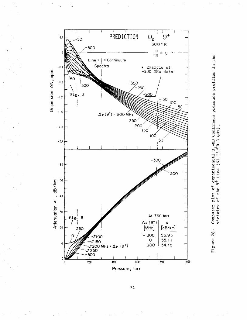
PREDICTION 02 g+
300 o K -300
Io N
= 0 Q)
Line T Continuum ..c: .w
Spectra ~ •r-l
E I rJl a. Q) a. ....-i
•r-l -0.8 z -3 4-1
<J 0 -250 1-1
p.. c: 0 2 Q)
VI -1.2 1-1 .... :::! Q) rJl a. rJl VI Q)
0 1-1 - 1.6
6!1(9+) = 300 p..
!3 :::! ~
- 2.0 •r-l 0
.w ........ ~ N o::t: Uc.!)
-2.4 Ul ("") ::E:: 0
10 o~l
If)
....-i....-i C\S 0
.W....-i
60 ~\.0 Q)..._,
s •r-l Q) 1-1 ~ Q) •r-l P-H
E 50 :><: aJ+ ~ 0'\
' 4-1 CD 0 Q)
"0 ..c: .w.w ~ 40 0
....-i'+-1 1:1 P..O
c: 1-1 :;.... 0 Q) .w
+= 30 .w ·r-l
0 :::! ~ :::::s 8 At 760 torr p.. •r-l
c: s C) Q) 611 (9+)
0 •r-l - a u :> -<( 20 [MHz] [dB/km] \.0
-300 55.93 N
0 55.11 Q)
10 1-1 (9+) 300 54.15 :::!
00 •r-l
"'"' 0
0 200 400 600 800 1000
Pressure, torr
74

c 0 -0 ::I c (1) --<X:
E a. a.
z <J
c 0 (/) .... (1)
a. (/)
a
60
40
20
EXPERIMENT vs I THEORY
02 300°K
61141 MHz 0
--I -N
Table 1
------ Io 0 N
0.8 torr/s
s = 1.2
0~--------------------------------------~
0.5
/ 9+(6v = -10 MHz)
-0.5
- ..
-1.0
· ...• ----·::>< ... x -- · · ·x . ~N -- . . ..,.,
------ ~- _.: ~ • ••.••••• II< .... . ... --- --- ----1.5
! Refractivity Result
-2.0
0 zoo Pressure, torr eoo Figure 27. Comparison of experimental and theoretical continuum
pressure profiles at 61.1406 GHz [~v(9+) =- 10 MHz].
75

0.6 PREDICTION 02 7+ /5- Doublet
300°K Q)
0.2 Io = 0 ,.c: -1-l
E N p a. 0 •r-l a.
CJJ
~ -0.2 Q)
r-1 •r-l 4-1
c 0 0 !-I (/)
0.. '- Q) ~ -0.6 !-I (/) ;:l
CJJ 0 CJJ .
Q)-!-I N
-1.0 O..ffi s ;:lC"'") ;:l • Po
•r-l -1-l +I
-1.4 p o...;t u .
0 t/) \0 ;:E:'-" I
70 Line+ Continuum
N 0
r-1-1-l Spectra ttl Q)
I -l..lr-1
60 p,.o Q) ;:l
I s 0
•r-l ~ !-I all
I O..ll"\ 50 :.:-aJ+ E
I
r--..:.:: 4-1
........ 0 Q) (I) ,.c: "0 40
-1-l -1-l
I 0
r-14-1 0..0
ts !-I :>-.
c 10 Q) -1-l
0 30 -1-l •r-l
+= At 760 torr ;:l p 0 0.. ·r-1
• ::::l !:::.v (7+) 5 .;:l c a Cl>
[MHz] [dB/km] u :> -- 20 <( .
-300 56.19 co N
_+150 0 56.46 Q)
10 _+200 MHz = !:::.v (7 +) + 300 56.17 !-I ;:l b.O
·r-l f.l:.<
200 400 600 800 1000 Pressure, torr
76
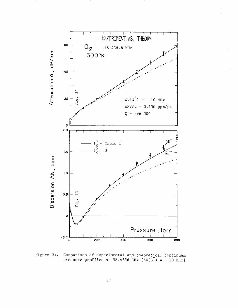
E X ........ co "0
~ c 0 -0 ::I c ~ -<(
E a. a.
&0
40
20
02 58 436.6 MHz
300°K
6v(3+) = - 10 MHz
6N/6t = 0.130 ppm/~s
Q = 396 000
oL----------------------------------------J 2.0 ,---r---r--r---r--r--..,.--r--;---,..~--r--r-.....,.-r--.,.......,
0 -- IN - Table 1
1.5 I 0 0 N
z 1.0 <J
(/)
'Q) a.
.!Q 0
0.5
Pressure, torr
Figure 29. Comparison of experimental and theoretical continuum pressure profiles at 58.4356 GHz [6v(3 ) = - 10 MHz]
77

•-
E 16 ~ EXPERIMENT A 10
[ 02 A" 12 .::rt:. VS ..- THEORY o .. / t THEORY ~ THEORY .. / 8 300 K .. / 10 "'C 12
./ NL'1BUS 5 ./ L ••
"' 10 / IS ./ . e
ts -~ t n 1. 5 ~/ i J // I IS - .
o ~_/rs = 1 . 2 ~ t .v ~ • ~ • Q = 360 000 -f z
~ LR= 0.292 km <{ 0 - --- - _____ J 0
0.40
E z.of -- I0
- Table 1 I M ~ N ~ ···-···- I 0 = 0
.. o.liO ~5 N ~ z <J ~ 2.0. //
o.zo
g I.O~ //. ~ I /.• c;; 1.0
"- 0•10 Ch. 5 05
Ch. 4 Ch. 3 ~ 58 875 MHz . 54 943 MHz l / 53 647 MHz 1/)
0 0 or. I I I I I I I I I I I I I I I 0 t I I I I I I I I I I I I I I ' 1 0 !10 100 150 200 0 100 200 - 400 0 200 - - 800
Pressure, torr
Figure 30. Theoretical continuum pressure profiles with and without interference at the three NIMBUS 5 oxygen channels (Sabatini, 1972).
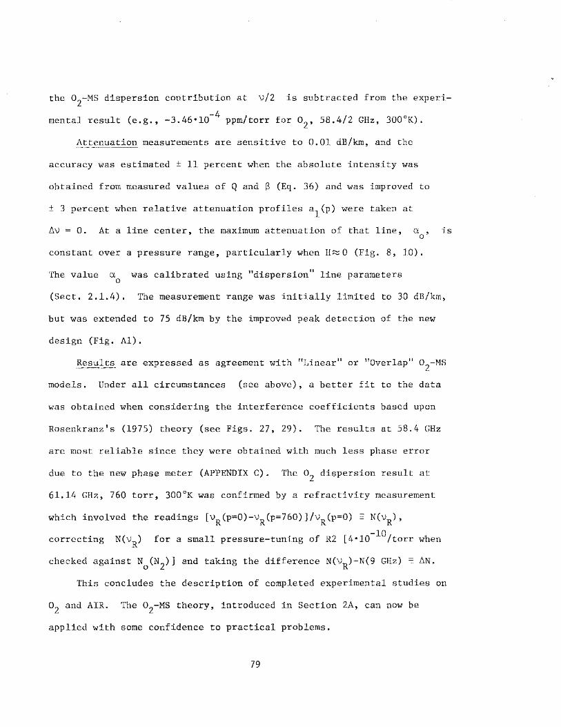
the o2-Ms dispersion contribution at v/2 is subtracted from the experi
-4 mental result (e.g., -3.46•10 ppm/torr for 02 , 58.4/2 GHz, 300°K).
Attenuation measurements are sensitive to 0.01 dB/km, and the
accuracy was estimated ± 11 percent when the absolute intensity was
obtained from measured values of Q and S (Eq. 36) and was improved to
± 3 percent when relative attenuation profiles a1
(p) were taken at
t..v = o. At a line center, the maximum attenuation of that line, a ' 0
constant over a pressure range, particularly when H~O (Fig. 8, 10).
The value a was calibrated using "dispersion" line parameters 0
is
(Sect. 2.1.4). The measurement range was initially limited to 30 dB/km,
but was extended to 75 dB/km by the improved peak detection of the new
design (Fig. Al).
Results are expressed as agreement with "Linear" or "Overlap" 0 -MS 2
models. Under all circumstances (see above), a better fit to the data
was obtained when considering the interference coefficients based upon
Rosenkranz's (1975) theory (see Figs. 27, 29). The results at 58.4 GHz
are most reliable since they were obtained with much less phase error
due to the new phase meter (APPENDIX C). The o2 dispersion result at
61.14 GHz, 760 torr, 300°K was confirmed by a refractivity measurement
which involved the readings [VR(p=O)-VR(p=760)]/VR(p=O) = N(VR),
correcting N(VR) for a small pressure-tuning of R2 [4•10-10/torr when
checked against N0
(N2)] and taking the difference N(VR)-N(9 GHz) = f:..N.
This concludes the description of completed experimental studies on
o2 and AIR. The o2-MS theory, introduced in Section 2A, can now be
applied with some confidence to practical problems.
79

B. ANALYSIS
2.5 Transfer and Emission Characteristics of Air (40 -140 GHz)
The transfer properties of the clear, dry atmosphere are expressed
through cumulative attenuation, phase dispersion, and phase delay along
a ray path h0
+ h1 (Eq. 43)- Part 1):
h,
[Np] , 6T = J6;d£ and T0
h 0
hl
J¢0
d£ [rad],
h 0
(58)
where a, 6¢(6N) are spectra of o2
whose dependency upon frequency v and
physical parameters p, T, H has been the main topic of this report
(df- path increment over which a= canst. and 6¢ =canst.; 1 Np = 8.686 dB).
The transfer function of the medium is defined by (Eq. 1- Part 1):
T = exp {- [A + j (T 0
± 6T)] } (58a)
Equation (58) is a filter function that governs the propagation of signals
through the atmosphere and can, in principle, be compensated by an equalizer.
Atmospheric emissivity due to molecular attenuation is commonly
expressed by a power-equivalent temperature,
00
I w (£) T (£) df,
h
(59)
where the kinetic temperature structure is T(£) and its weighting function
is
W(£) = a(£) exp (-A) (59 a)
Equation (59) represents a random noise signal that (a) determines the
ultimate detection sensitivity of a receiver and (b) is basic to
remote sensing atmospheric temperature structure T(£) by radiometric
means. The weighting function shows band pass behavior filtering
T(£) selectively with alti.tude as a function of frequency. The
solution of (59) requires height profiles of pressure and temperature to
80

calculate a(~). At selected frequencies v and v ± 0.1 GHz between 59
and 50 GHz, we demonstrate in figure 31 the variability of a (and 6N)
for pressures up to 800 torr at temperatures between 200 and 300°K. The
V are those chosen in NIMBUS 5 and future TIROS N satellites for temperature
soundings. The results are for the "Linear" 0 -MS model, although they 2
may be converted to the more probably "Overlap" model using equation (57).
Weighting functions have been calculated at frequencies between 50 and
67 GHz, usually for the U.S. Standard Atmosphere 62, by many workers
(e.g., Meeks and Lilley, 1963; Poon, 1974; Malota and Stein, 1974).
Two simplifying assumptions can be made to make W(~) tractable.
These are
i) p(h) p exp(-h/H), H = 0.0293 T o a
(e.g., scale height H = 7 km when T = 239°K); a
(59b)
(59 c)
(pressure and temperature exponents x, y for small variations of
p and T are listed in Table 18).
The altitude range over which W(~) is significant determines for an
opaque (A0
> 3Np) atmosphere the weighted mean temperature TA that
can be received. With the help of(59 b,c) one can calculate the parameters
that govern the maximum w. These are {Poon, 1974) m
the pressure p = (x/aH)l/x , (59d) m
the height h = (H/x)ln A (59e) m 0
the attenuation a = x/H , (59 f) m
and the opacity Am = 1 [Np] . (59g)
81
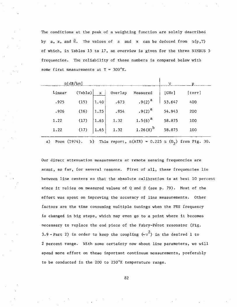
The conditions at the peak of a weighting function are solely described
by a, x, and H. The values of a and X can be deduced from a(p, T)
of which, in Tables 15 to 17, an overview is given for the three NIMBUS 5
frequencies. The reliability of those numbers is compared below with
some first measurements at T = 300°K.
a[dB/km]
Linear
.925
.926
1.22
1.22
(Table) x
(15) 1.40
(16) 1.25
(17) 1.65
(17) 1. 65
Overlap
.673
.854
1. 32
1.32
Measured
.9(2)a
.9(2)a
1.5(6)a
1.26(8)b
\)
[GHz]
53.647
54.943
58.875
58.875
[torr]
400
200
100
100
a) Poon (1974). b) This report, a(AIR) = 0.225 a (02) from Fig. 30.
Our direct attenuation measurements at remote sensing frequencies are
scant, so far, for several reasons. First of all, these frequencies lie
between line centers so that the absolute calibration is at best 10 percent
since it relies on measured values of Q and B (seep. 79). Most of the
effort was spent on improving the accuracy of line measurements. Other
factors are the time consuming multiple tunings when the PRS frequency
is changed in big steps, which may even go to a point where it becomes
necessary to replace the end piece of the Fabry-Perot resonator (Fig.
3. 9- Part 2) in order to keep the coupling ("'v2) in the desired 1 to
2 percent range. With some certainty now about line parameters, we will
spend more effort on these important continuum measurements, preferably
to be conducted in the 200 to 250°K temperature range.
82
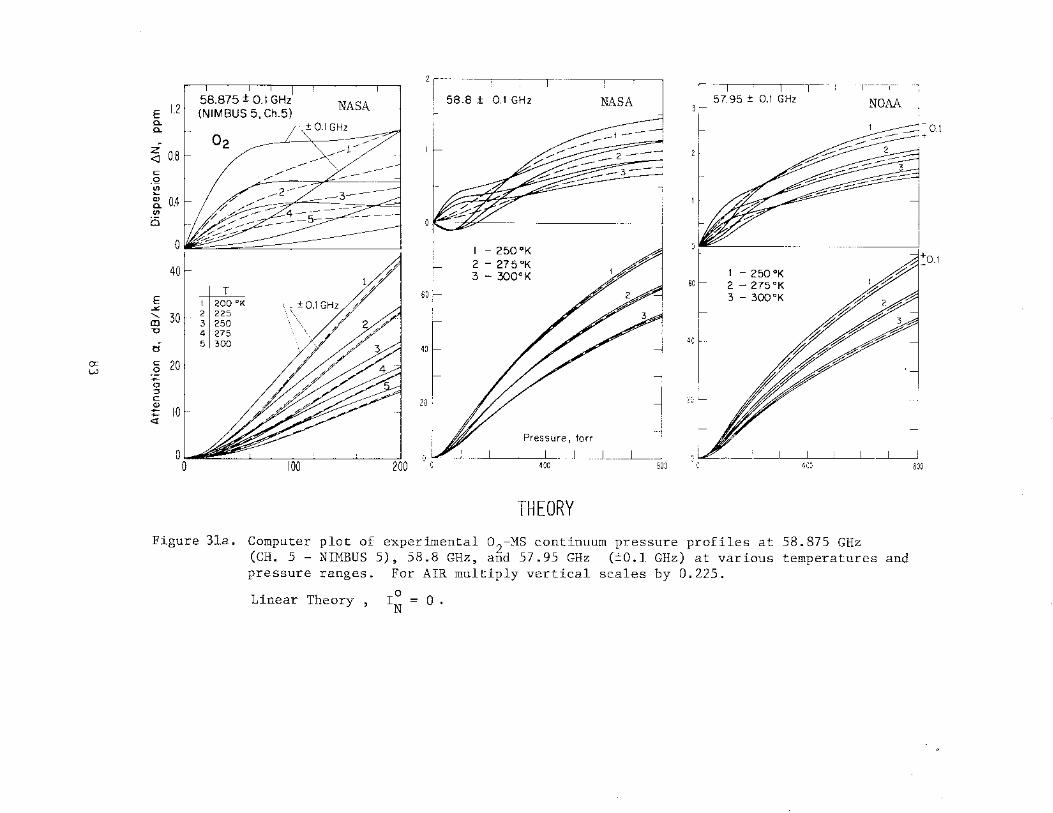
CXl w
58.875 ± 0.1 GHz' I I 58.8 ± 0.1 GHz NASA 57.95 ± 0.1 GHz E I.T (NIMBUS 5, Ch.5) NASA
~ ~ I ~=-j I ~-0.1 ~ 0? . ..-.-- + --z
<J 0.8 c
.Q (/) .... ~ 0.4 (/)
Ci
0 I - 250°K
401- /1 60 ~ 2 - 275°K
7~ 60 r 3- 300°K 1 - 250°K
T 2 - 275°K
] ~ ' 200"' . -. --. 3 - 300°K
' 30 2 225 CD 3 250 "0 4 275 eJ 5 300 Y7 // J.:;:/1 40
g 20 -0 :::l c I /P~£/~~1 20 L /// 10 ~ 10 ~
0 0 0 00 0 100 200 400 BOO 400
THEORY Figure 3la. Computer plot of experimental 02-MS continuum pressure profiles at 58.875 GHz
(CH. 5- NIMBUS 5), 58.8 GHz, and 57.95 GHz (±0.1 GHz) at various temperatures and pressure ranges. For AIR multiply vertical scales by 0.225.
Linear Theory , I0
= 0. N
BOO

4
t 54.943 :!: 0.1 GHz
[ ± 0.1 GHz 1 ~ ~ 54.96 ± 0.1 GHz 1•w~±0.1 3
(NIMBUS 5, Ch.4)
o. 3L ~ __.--j ~L ~~ o2 z <l c: 0 .§
"' 0. .!Q O, l o/' __ ~
0
30 f- 1 - 250 OK f 1 - 250 OK 2- 275oK 2- 275oK 15t T
E ~ 3 - 300°K 3 - 300°K 1 200"K ~ 20 2 225 ~ 3~
4 27:; r:i 20 10 5 300
c: co ,g -~:- 0
~ 10 ~ ~ ~ 10
~7 I 5
0 0 •• o~~~--~---L---L--~----~--~--~ 0 400 BOO
Figure 3lb. Computer plots of experimental o2-Ms continuum pressure profiles at 55.5 GHz, 54.96
and 54.943 GHz (Ch. 4 -NIMBUS 5) (±0.1 GHz) at various temperatures and pressure ranges. For AIR multiply vertical scales by 0.225.
Linear Theory , I~ = 0 .
400
GHz,

CXl V1
5 r-
53.647 ± 0.1 GHz
E 4 r (NIMBUS 5, Ch. 3)
a. . 02 a.
50.3 ± 0.1 GHz NOAA
-z <J c 0
~ Q) a. {f)
0 .
0
~ 20
1 - 250°K 2 - 275 °K 3 - 300°K
1 - 250 °K 2-275°K 3- 300°K
...... CD "0
l:l c 0 ~ 0 ::l c 2 ;;:{
r
T 1 200°K 2 225 3 250 4 275 5 300
10
00 400 o o~~~~L_ __ L_ __ L_ __ L_ __ L_ __ ~~
BOO o 400 aoo o 4 oo aoo
THEORY Figure 3lc. Computer plots of experimental 02-MS continuum pressure profiles at 53.647 GHz
(Ch. 3 -NIMBUS 5), 52.8 GHz, ana: 50.3 GHz (±0.1 GHz) at various temperatures. For AIR multiply vertical scales by 0.225.
Linear Theory , I~ = 0 .
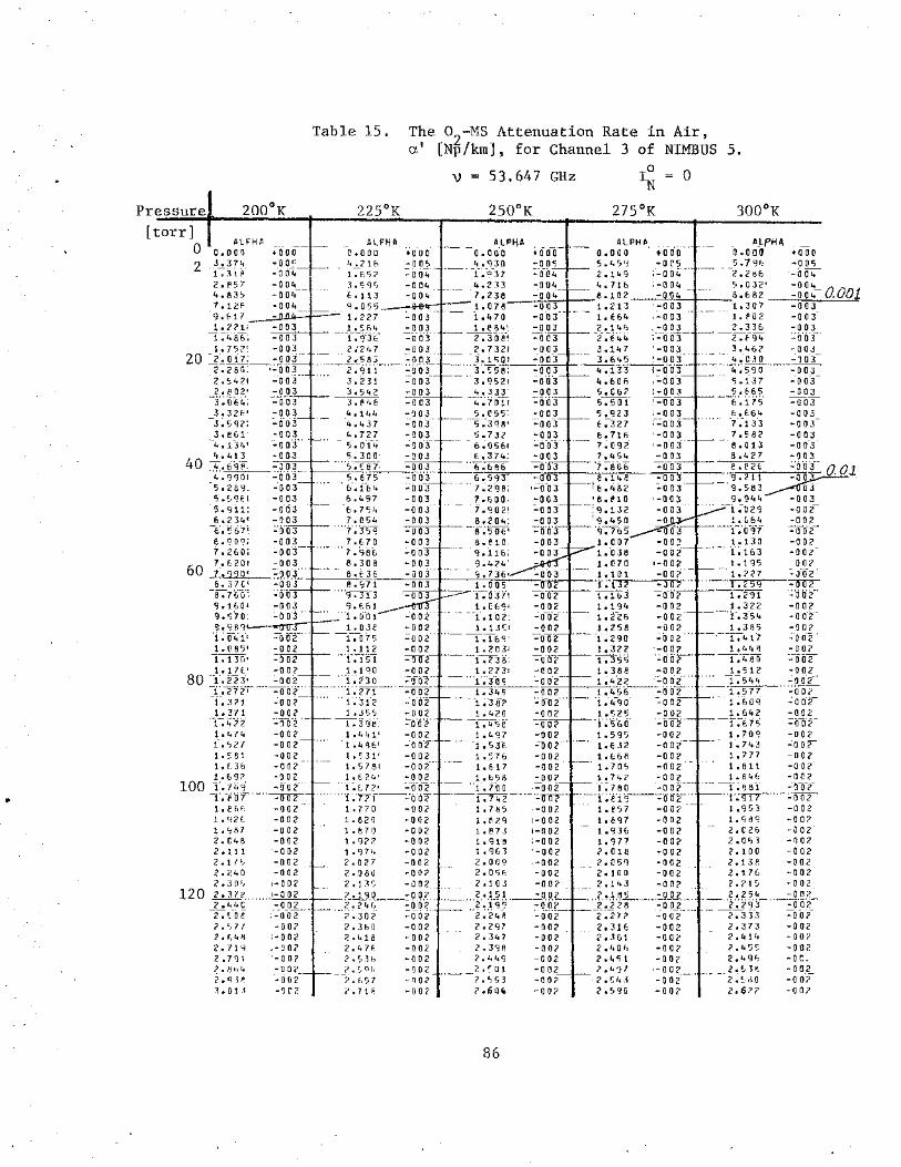
Table 15. The o2
-Ms Attenuation Rate in Air, a' [Np/km], for Channel 3 of NIMBUS 5.
" = 53.647 GHz Io = 0 N
Pressure 200°K 225°K 250°K 275°K 300°K [torr]
HFHA ALFtjA __ ALPHA AJ.PHA 0 o.oon Q. 0 0 0 --o. o a· a +000 o.oo() +000
2 3.374 . ---"-'--216 4o'l30 -005 ~. 796 -005 T;-Yti' 1.652 -T-.-9-3 7 =-o·o 4 --2.286 -:i)Q4 2.e57 loo233 -004 ~. 0 32' -004 4.835
--7,238 -o o4 8,682 -oo4 0.001
7.12~ 1.078 -003 1.307 -003 9of17. 1.4 70 ---0 0 3- 1. eo 2 -0 0 3-1. :??11 1.~&'+ -a 03 2.336 -003 1~486; -1.<?"J6' --:a 0 3 -z:-fq<; -=oOT 1.752~ 2 i24 7 2. 7 321 -003 3,4&2 -003 -20 2. 017: 2 "5 83 3.1 ~ o 1 =-a·o-3 ";c 3 o ~ 10_3 __
2. 2 eo: 2.911 3. o5a:---003 '+.590 -003 --2. 5 421 3. 2 31 3.9521 =oo3 5.137 --oo3-2. eo 2' 3.542 ". 3 33" -003 5.6&5 -003
3.oo4-: -~ ~ -003 -&-.175 -=oo3 3. 32E:' '+o1'+'+ s.055~ -003 6,H4 -003
-3.592: 4,437 5.~3.~8' ::oo3 f.-13-3 -003 3. e& 1- - .. __. 7]_7_ 5. 7 32: -003 7. 5 82 -003
--,. .134• 5.014 & :o5&1 ~lf03 8.01J -o o-3-
40 4.413 <;,300 E:. 3 7'+: -003 8.'+27 -003
4.69"F -5.587- &.686 -003 e.en -oo3 0 Ol 4. 9901 5.675 6 .993" -003 __ 9.211~-5.289: -o-:H,,. --7:298: ·=-o·o3·- 9,';83 03 5 .59EI &.457 7. 60 o. -003 9.944 -003 5. 9 i 1: 6.75'+ -:.oo3 ---i :o29 --o 02-& • 23'+' 7.054 -003 -002 -6.?67~ -?--;-T59 -003 -002 E:. 90~; 7ot70 -003 -002 7. 2& o; -i.-e; a& :a o-3 -n 02-
60 7. 6 2 01 8.308 002 z •0 90' 8 ,f 36 -~ J-02-6. 37C' 8oC)71 ~
-a;·n,o; -9.313 -002 -002 9 .100< 9.£&1 -002 -002 9. 5-?o- L0-01 =-o-02 -oo2 g.989 1.038 1. 13 ~· -002 -002
1--;--o,.-f, =--o 02 -c-o75 -=--oo2 ~-o o2-1. 0 85' -002 1 o112 -002 -002 ~ -ao2 ~ -=--oo2 ::002 1o17E' -002 1 ol 90 1. 27 31 -002 1. s 12 -o o 2
80 ·1--;-223• -:.ao2 -r--;- 23 0 --f-;To·g ~0 lf2 l--;-544 :oo2 1 .272 1 -002 lo271 1.345 -002 1.577 ------=-oii2 1.321 =-iltl"2- - i--;-312 --1.-3 82 -=--o·o 2 --i--.-609 ::a o·z-1.371 -002 1 • 3 s 5 1,420 -002 1.642 -002
1.'+22- :'fOZ- ----y--;J <J/1: ~..---rr -002 ~7<5 -=ooz 1o474 -o o 2 1. 4 41' 1 ,t.g7 -oo2 -002 1.527 -o o2 -- f;-4 ~6' "1. 53£: -ll 02 -·ooz 1o581 -002 1. 5 31' 1.570 -002 -002 1ot36 -002 1. s 7 81 1.617 -002 -002 1.692 -3 0 2 1. t 24' 1.658 -002 -002
100 T~·7£fg- -fio2- -r:u2• - 1. 7 0 0 .::-a oz ~Yo2
1. eo 7 -002 1. 1 -1.742-- -0 0 2 . 1.€6(; -002 1. 77 0 1.785 -002 1o92t -002 1.820 1. e 29 1-0 02 1.98~ -002 1o':87 -002 1. B70 1.873 1-0 02 1.936 2.c26 -002 2.C48 -002 1. 922 1.918 :-0 0 2 1. 977 2.0<;3 -002 2.111 . -0 0 2 1. 974 1. 963 ·-o o 2 2.018 2 ol 0 0 -002 2.175 -002 2.027 2.009 .-o 02 z.c?q 2.13 e -o o 2 2.240 -002 2o080 2.0<;6 -002 2 o1 00 2.176 -002 2.30S ,_ 0 0 2 2.13S 2.1 0 3 -002 2,143 2.215 -0 0 2
120 _2.372 __ <-002 2 ol90 2.151 -oo2 2.185 2.25'+ -002 2 ,l,4 c -002 2.246 2 .199 ---=-a o 2 2. 2 28 2.293 -o-02 -2---:(oe :-o·o2 ~302 -2:-i,.IJ --=-oo2 -;i;2 7 7 -?~JJ-3 =--o-oi> ?.577 -007 2o3b0 2o297 -002 2.316 2.373 -002 2. f,4~ :-0 0 2 2.418 2.347 -002 2.301 2.414 -002 2o71g '- Q 0 2 2o47f. 2.398 -002 2.406 ?,4!>? -002 2. 791 . -0 0 2 ?.5.16 2.449 -002 2.451 2o49fi -o c c
? • e;;4 -o o 2 _ __].t:.qr) 2.~01 -_o o 2 ?,4'37 z.~l~ -oo~ 2. <).lP. ~- 0-0 i ?.b57 2.S53 -002 2.~43 2,!-:dO -0 02 3. 0 1 .l -~C2 2o71F, 7 .!)00. -007 2o59(j 2.6?7 -00?
86
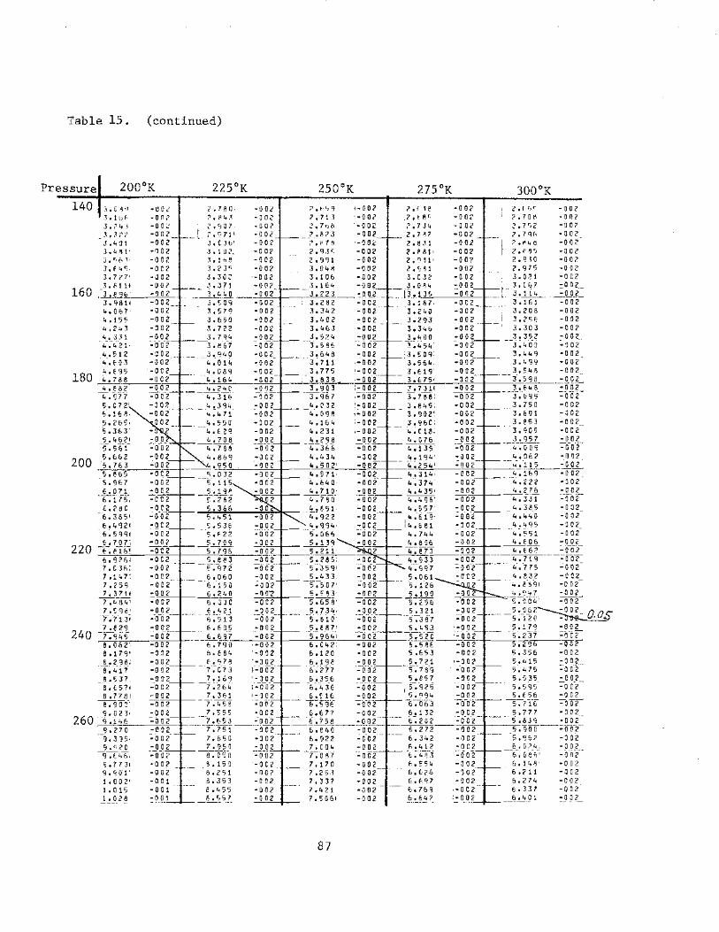
Table 15. (continued)
Pressure 200°K 225°K 250°K 275°K 300°K
140 3. (; Ji\l -uo~ ? • 7 A tJ, -002 ? ,t·?g •-0 07 ?.fH -002 I c. r f)r -00? 3. 1 hf~ ? • tl4.'~' -002 <. 71] ·-o o? ;c, t A~"· i ? • 7 0 ~ -00? J. ?4.( <. 90 7. -00? ~.7h8 ?.7J4 2,7S2 -u o? 3,.3('? ?. ~· 71 1 -002 .?_.A 7 3 2.7-V ? • 7qr, -002 J.401 J.C3b' -002 ;", t'17 R 2.831 ?.~40 -002 3. 4 -~ 1' 3.1 u 2. -00? 2.<J.J~ 2. p 81' 2. e B r) -002 J, r.6.1• 3.1h8 -002 2.991 2. ") 31 1 2.~10 -002 3. f 4 r;. 3.23~ -002 3.04M 2." 81- ?.975 -0 0 2 3.7?7' ;!. 30 ~ ·-0 0 2 3.106 3.C32 I 3. 0 ?.1 -002
160 _3.f111 3.3?1 -002 3.164 --~-.0~4· 1
_ 3.L67 -002 , 3 .e9o: -002 __ 3. 2 2 I __ :__Q_Q.£_ 3.135 . 3.114 :_QJJ 2-
3. 9811 s.soq -002 .. 3.282 :3.187· 3 .t 61 -002 4. 0 6 7' 3.579 -002 3.342 3.240 3.208 -002 4.155 3.650 -002 3.402 3.293 3o?St -002 4.243 3.722 3.463 3.346 3.303 -002 4.331 _ 3.7q_4 3.524 3.400 3.352 -002 _
. 4-:-4-21' 3.867 --3.5 86 T."45i; --3:4 oo -ao2 4.!:'12 3,940 3.648 :3. 5oq: 3.449 -o o 2
. .,--. f 0 3 4.014 3~711 3.564- 3.49<;) -o o 2-
180 4oE95 4.089 3.775 3 .619. 3.548 -002 4·. 788 4.164 3.8B 3·.675' 3.598 -002 4.1!82 4.24C 3.903 ~. 7311 3.f48 -:.ooz
4.9Ti -"4.316. ""3.%7 3. i88": --3:69s· -:a·oz-5. 0 7 2' 4_,3'34 4.C32 3. 845: 3.750 -002 .; .16 a. 4,471 4.0<)8 3 .<J02' 3.601 -002
__ 5. 265· 4.550 4.164 3. 960: ... 3.853 -002 5 .363" 4, E 29 4.231 -.. ~ c 18: 3.<J05 -002
__?_. 4_~2~ _ 4....I.Q_8_ 4.298 4,C76· _}_~ _ -002 5.?61 4.788 -~;-:-:366 4.~ 4.00~ -=-o-aT
200 5.662 4.434 - 4.194' 4. 06 2 -002 5.763 4. 502' 4~254' - .;.-115 .... 0 02-
5.865 _4 •_? 7_1' 4. 314• 4.169 -002 5.9€:7 .. -;.374. - ·-.;. 222 -002 E.071 4 .435• 4,276 -oc2
6.175. 4 .496' ~31 :002 E. 2 8 0. 5.366 4 ._55]' 4. 38_5 -002
--6.385' 5 • .,51 4. c 19 1 4.4'+0 -002 _6_.492< 5.531': it. .681 4.495 -002 6.5991 -S,F22 .. ;744 4.551 -0 0 2-
220 Y...! 7...Q.z..; 5.709 ". e o6 4.~06 -002 ~. 816~ -5-:7% T.Do ~&2 -002 6.9261 5.883 ... ~33 4.719 -002 7; c 3fo: :.CJ72 .. -;·r:,gt 4,775 .:o 02-
7.14 7: 6.060 5.061 .. 4,832 -OC2 7. 259. -E:.i-50 s-:-126 4.e"5'll ;0 02-
_l_._3_7__1_1 6.240 s. ~ 8 3• 5.190 -~~~'.'+.I_ -002 7 .~ 84 1 6-:-330 -s~s-8• 5,256 5.004 :ooz-7. ~ 96 1 1':.421 5. 734• 5.321 _5._0_62~
--r.-7131 6,513 -s-:-eio· ·-s-:--3 81 5.120 - '
_?~€?.'!.. - 6.1':05 5. e a 7• 5.453 -002 240 7 .9<t5. 6:697 ·-s-;9&41 -s--:-5-zo -o 02
8. 0 62: 6.790 6. c 4 2: s .sac -002 8 .179' 6.e84 l).120 5.653 -002 e .295; -· 6.<J78 6.1'38 5.721 -002
··a:-417 1-:c 73 6.277 ~5:7a·iJ =-ooz-8.537: 7.169 6.356 5, f·S 7 5.53? -002
-8;£571 -7:264 -6-;-4 JE: It-~~~ - --s . s·g·s- =-o c-2-
8. 7781 7.361 6.~16 5, E 56 -Q02 --e:9oY· -T.:-458 6.59(: 6;0-6-3 ~716 -=-ow
9. 0 2 3· _]_!~?~5 6.677 6.132 5.777 -002 260:-'.l.T46 -~. 758 e.-;2o2 --.;-.8JCJ :oo2
g, 27 0 6.840 ~-- 5.900 ---002 -'3.335· 6.922 6.342 5.%? -002
g.<, 20 _r_._c 0_4 _6 !_4_!_2_ 6. 0 24. -002 9-:T46. 7,0R7 6.4~3 6-; Ge-6' :a-oF ". 7 7 31 7.170 fo.~54 6.148. -002 9. '?0.1! 7. 25.3 6,626 6 .?11· -OQ2 1. 0 0 2' 8.353 7.337 (;,f'l7 6.274 -002 1. 0 15 8.<t55 7. 4 21 6.7&9 6.337 -002 1. 0 28 -~"c5.!_ 7.5061 6.e<tz 6.401 -0 0 2
87

Table 15. (continued)
Pressure 200°K 225°K 250°K 275°K 300°K
8. ~6 0• 7 .~ gf. 6.4E:4 -0 0 2
8.764 7. f. 77· 6 .528· -0,0 2 e ;eo e --;-.-7&2· 6 .sgz· ·002 8. g 7 2' 7. 84'31 6, E 5_& -0 0 2
g. 0 77• 7-~~35' 6. 721: -=-o 02-
g .182 8.022 6, 7 8~ I -002 ----g-,z!la- a:log -E;855< -=aoz
1.1341 9 .3'35 8.1'37 --f:. 916' -002
T~1i.~ '3.502 ·e-;285 7.~05 6. 981' -o o2
300 1.161 9.609 8.373 7. 5 81· 7. 04 7 -002
1~75 g~ 717 '8: 462 7~-t%• -7;112' -o o 2-~80 g,e25 -a-.--551 ---r;rrz- 7 ,i]gl -ac2
~3 -------g--,---9-;li;' --a;EI;'O ·7-;-ell't' -7-;-~>45; :Oo2
1.21E 1.G04 8.730 7. e 84· 7. 311' -002
1--; 2 3 G 1. CIS ·a; uo -7. 960' 7 • 3 7 ~I -oo2
1.244 1,G26 8.''l11 8.037 7 ,445. -002
i.2se 1,037 9.G02 8.114 7. 512' -o o 2
1. 27? 1,G48 9.093 8 .1 '32 7 G 5 79' -o o 2
1. 28-7 ----r:rs i 9:184 87269 --r-:&4T -0 c 2
1.301 -o o 1 1. 0 7 0 g .27• 8.347 7. 7151 -0 0 2
320 1.315 :.oo1 1-. G8 2 q ~3&8 8.425 7. 7 82' -0 0 2
1_._329 -o o 1 --1. G g 3· 8.504 7.851 -0 0 2
1.344 ~001 1 ~ 1 a 4 0~582 7.919 -0 G 2
1.35~ -001 1 .1 tE 8.E61 7.988 -0 0 2
1,37 r :001 ~ji - e--;-?t;o 5':056 -=DoT
1.387 -001 1.13'31 e.e2a 6.125 -002
f.4 02' -o oi (, (SG! 8.900 e.1'34 -oar 1.417- -001 1. 162: 8,<;8G e.2&4 -002
T;i; 32 -=-oaT --1;·173', g;o&o 6-.3 3 3 .:a o 2 -
1.446 -001 1.185: 9.14C 8.403 -0 c 2
340 1,1.61 ·001 1--;-T9fi 9.221 a.473 -:oTr 1.476--·001 1. 2 0 81 9.302 ·-e;-s43--:00Z
-1~-49·1 :·oaT -f;czo< 9.383 8.E:(l, -0 0 2
-
1. 50" ·001 1.2321 '3.465 8. 684' -002
·l.s 21 -=-obi -1-.244; - o1 9.546 - ·e; 7 55 .::o 0 2
1.537 rOO! 1.? 56' -a '3.628 ~.e2s -oc2
1.552 ~001 1-.-?&T -=-o o 1 9.710 -e-;egf -;:ooz 1.567 ·001 1. 2~ o: !,C'!~ -001 <J.7'33 8.'!68 -Q02
i .58 2 ;;iliJI ·--r; 2 92 -r;loe ;~01 g;876 - g·, Q 4 0 -·o o z
1.5<)8 ·001 1.30 4 1.! 18· .-o o 1 -002
360 -1 , E 13 -001 1 .316 1.12e ·.:.ooC -002
1.E29 -o o 1 1. ze 1.138 '- 0 0 1 -002 1.E.44 =-o o 1 -~-:-·3-40 -r.ne :=a o 1 -;:ooz 1.E60 -a o 1 1.352 1.158 •001 -002
1.676 -QOI 1,365 1.168 -001 ..
~. '• 7 2 -002
1. e,g 1 -001 1. 377 1.17 p -001 1.046 g.s45 -a o 2
1.707 ·001 1.H9 1.188 ·001 '1. 0 54 q. C18 -002
1.723 -001 1.402 1o198 ·001 1.063 ~.6~1 -002
1. 7 3'3. -001 1. 414 1.20~ -001 '1 • c 71 <).765 -002
1_. 755' -001 1. 4?7 1.21~ -o o 1 1. 0 ~ 0 <),838 -002
380 1o771 -001 1.43<J .228 1 1.086 -0 0 2
1. 7 8 7; ·001 1.452 1.239 -o o 1 1, G g 7 -002
• 1 • eo 3. ·001 1.464 1.?4'3 ·001 1.105 -0 0 1
J_,JJ_g• :09_~ _ _!__,_ ... 7_7 1.25'3 -001 1.114 1.013' -001
1 a 8 3 ~I -001 1. 4 g 0 1;2i;g ::a o 1 -c:123 -i.c?o·~ 1 '8 tj 1' ·001 1.?02 I •? ~ 0 ·001 1.t.H loG?~ •001
1.P6e •001 1.?1S 1.Z<JO ·001 1 .t 4 0 1.05? - 1
1. e e4 -001 1, r 2 ~ 1. 3 01 -001 1 a 14 ~ 1,C4l -00 •
1. ~ 0 0 ·001 I , ~ 41 1.311 ·001 1.15 7 11J 0 50 -0 01
1_._';1 1 7 :O 01 1,S54 _1 • 3? 1 ·001 1. !6f, I_~o s • -OO_L
400 1.~33 -001 1aS67 I, 332 -ooT 1. 1 7? 1.06S -001
88
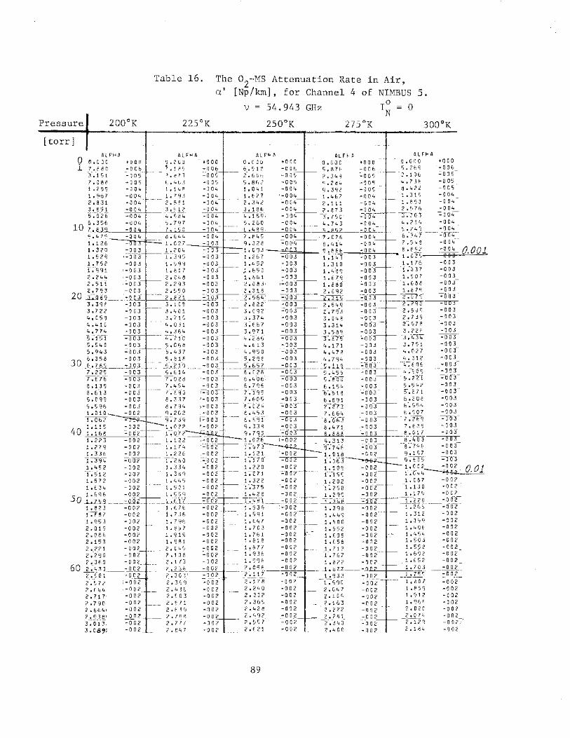
Table 16. The o2-Ms Attenuation Rate in Air, a' [Np/km], for Channel 4 of NIMBUS 5.
\J = 54.943 GHz I~ = 0
Pressure
[torr] Alf'HA
0 o.ooo 1 7.eso
Y:1s1 7.08~
1 • 2 5'3 1.967 2.831 3.851 5~-lf26
+000 ·OOb -_ 0 0 5-
•005 -00<, -00<,
ALFHA 0 • c u 0 1.1~') ? • b 71 L,<,~J
1. 1 "p 1.7'33 2.581
~~'-+-- 3.512
A L fl- A +0 0 0
'•006 -a os--o OS -oos· -004 -0 0" -DOLo -:o~
10 ~::~~--~~~--~~LL--~~L+--~~~--~~~--~~~ -004 -0 04--004
30
C?.47~ 1.126--~~~4=~ 1.;320 l.ffi 1.752 1.'3'31 2.244
-o o"-~0001. e e J • -o o 3 -oar -003
•-oo3 -;;oor -003 -003 -oo3 -;;-lroT -003 -003 =-oo3- -oo3· -003 -003 .;003 -003 -003 -003
"·<'if& -003 -003 <,,t13 -003 -003 ;.-;i:i50 -oii'3 -oo3-s.zse -oo3 5-.657 -0-03
7.225 6.~26 -003 T:EIT 6-;-.:;or. ~o· 03 8.13'3 6.796 -003 8;613 -aor s.ogg 6.208 -003 s·;-,;·9& -&-.ss" -oo3 1.010 6.S07 -003 1 , C b 2 ---~M--- :-;:..;;--+-- -7 • i?t S -=103 1,115 7,E3S -003
40 ~1~·~1~6~e_·--~~~----~~-~~~~~~~~---~~~~--~~~---~~L_+-__ -~e~~~o~1~7 ~ao3-1.223 ·-002 1,026 8.403 -003 T~27s ·-=-ilii'2 r-;-o73 --8-;?C;E: ~oo3-1.33& .-002 1.121 9.197 -003 1~94 .-ao2 T;Tto g,t05 ~Y03 1 • 4 52 -·o o 2 1. 22 o 1. c c < ~-o a 2 0 01 -1-;s12 ~oo2 r;271 -r;o-.4~ 1.572 1.445 -002 1.322 1.087 -002 1 • t3 4 1. 5 J1 - il 0 2 J.'.-37 5 ' '1 • 13 0 - 0 0 2
50 r-:~i~ __ .::.JJ.J.L<.-+- 1.55'3 -002 1.428 1.1i5 -002 _ 1.< _ _:~::.!o!Jo!-'-2~ __ _!T'-'~'-'"-~el..!T"_--:·-=-~o~o-~z-l- --y;-z-zo ::aa2-
1.823 -002 t.OE -oo2 1.53.; :-oo2 -oo2 1.2&5 -002 1-;e-87 -002 i-.73& -002 1~5'31 .-002 1.44" -002 1.312 -002 1.953 -002 1.796 -002 1.647 .-002 1.500 1.35<) -002 2.019 -002 1.857 -002 1.703 -002 1.552 1.40E: -002 2,086 -002 1.919 -002 1.761 -002 lotOS 1,Lo5t, -002 2,153 ·OC2 1,981 ·002 1.618 -002 1.&58 1.503 -002 2._?.21 -002 ____ ~_.045 -002 1.8_77 -002 1.712 1.552 -002 2.2<Jo -oo2 2.1oe :.o-o2- 1.936 -·oo-2-- i.-.767 1.6iJz -oo2 2 ... JF>O -oo2_ 2,.1 73 -oo2 1.9% ~oo2 . 1.cs2 -oo2
60 2,430 -002 2,23& -002 2.osc -oo2 1.703 -002 2 • 5 o 1 ---_a .ll. 2 2 • 3 o 3.~ .::._""a""o""2+-----;2"".c.;1:c;1:.;;7 ---- o o 2:-t----'-'..a..J'-'- ·"'"0LJJ0L<2'--.J---'1~7~5~c ----::ooz
HE ;:::: ~mtTm 2.S72 2,ft,L 2. 71 7' z.?CJO z. 66£,1
.?~3.§.' 3, 0 1 ~I 3. 089<
2.571 -002 1.96~ 2.t1~ -oo 2 ·- 2.020 ~_,_?CJ.P, -0 02 ~.7.4
2.777 2.557 ~-oo 2 2.1zg 2.847 2.£21 -~07 2.181,
89
-0 0 2 -002 -002 -002 -002 -002 -ori21' -002

Table 16· (Continued)
Pressure 200°K 225°K 250°K 275°K 300°K
70 3.165 2.~17 2 ,(,8 7 2,41;1 t' e ('l4 0 I ·-o c2 3. 7'•1 2.c;r.1 2.7~2 2.?22 2 .?96' •002 3.3!R J,O~M 2. e 1e 2.S8J 2.353. •·0 02 3.395 3,11 0• 2.885 X•c45 ?.410 -on? 3~47 3 J • ?O.'; 2.46 7r: -oaT 3.!>5? ~.5?5( -a o 2 -3. f J 0' ? • ~ p J; -0~2 3,710 2 .f.41 f -002 3.789 2o700 •002
so _h~"- ?.75~ ·OC2 z~aie ::Oif2
3.1<;1 2,87fl
! 3, 216 2.'33f
--·- 3.281 ?.998 i3.34t 3.05~
3,41? 3.120 T-:4-71! 3~-f81
3.544 3.242 3-:&10 3.304 3.&77 3.3&~
90 ·-3.428
4.427 --4.500
4.573 5.462 4.6<tE
100 5.5_4'? 5.f;36 5, 724 s.eC2 ·;;ao·z-S,'JOO -002 s;-c;a-g ·002 6.C78 4.3e2 -ao2 6. i&7 ~-~ 44 7 . .:-o-o2 6.2~E: 4.512 ·002 6.346 -;:;.~77 ··OOZ C o-436 ~~ ... ~ :-o o 2
110 6:~?6 4,707 ;:;ooz 6,H7 ~-
&~708- 4-~8-38 -.;~02
c.79~ 4o'J04 '·0 02 {;e9c . 4-·~"tf6g '-oaT
5.035 .-o 02 -s-:-nJI-~
•1
5o1&7 •002 -&~141 5; 2 :!J ,:. - 0. o.s 6,217 · So29~ •002
120 1;;293 i 5;365 ;;0_0_2_ 6.369 15o<t31 -002 6.445 5.497 -002
7.72'+ 6.522 s .5&31 -002 7--:--817 ·r:.-:598 1 s·:{zs -~ocr 7.912 E:. €:7'+ !s.&<?E: ·-a 02 8 ~To6 £:-.751 : s·-;762 .:-a 02 e. 1 o 1 6oP27 js.tze 1•0 0 2 8;196 1J~<flf" :s;-e95 i-ooz 8.291 7.559 &.931 !So9o1 •-0 02
130 ;;is~ - 7~{4-3 G57 21:. ~-002 8,482 7.727 7,134 -002 e.578 'f.-812 7 ;211 •002 8of74 7.696 7,?38 -002 il:?fil -r:-<J8T 7.365 ::002 8.8~7 8.0&6 7,442 ~.360 •002 8o9o4 8.151 6.95~ &ol.27 ·002 <),0<;1 8.236 7.02~ 6.494 -002 9 .158' 8.321 7,f-74 7.10 I &.~60 -002 9, ?Sf: 8. 4 0 71 7,751 7.172 6 ,_£_27 -o 02
90
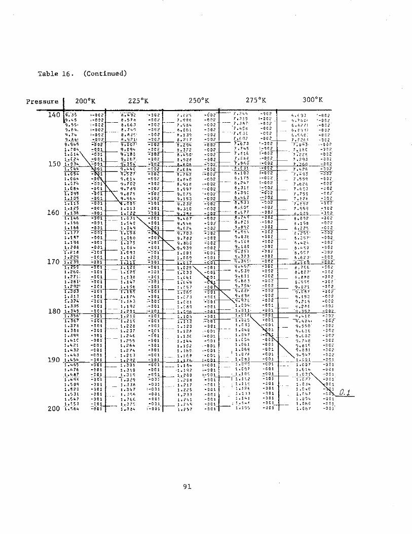
Table 16. (Continued)
Pressure 200°K 225°K 250°K 275°K 300°K
140 -r.-35 -8-.T<l2 ?.tee; -ooc 7.244 •Q02 F). ( g 3' '- 0 0 2
9.~5 e.57tl ?.C:OE: -OC2 7. 31 5 1-0 0 2 f,. 76 01 . -0 0 2 9.55• &.E.oJ 7.S84 -002 7. 3 8 7 .-o 02 6. h2/( '- 0 0 2 9. f-4, e.H'l 8.061 -002 '7. 4:: ~ -002 . - 6. e Y n -o o 2 <J,74 8 .13'l -002 . 17. ~ .J (, -002 &,Si,Oc -002
8.217 -002 7. (. 0? -002 -002 e,-zgt;" '7:673 .-o o 2 8,372 '-3 0 2 e-;45o· -o o 2 a.52e -002
-0 0 2 ----~o~o-2
~o-oz
-002 7.62C -0 0 2 7.tCJ3 -002 7.75'i -o oz· 7.t2f: -J02
-7-:Ts2 -o o 2 -~02
160 __ ::;oo2 -002 ·-o o 2
8.22~ -002 .. e. c'i 1, -:ooz
-001 8. 3 57' -002 ·.;o o i. 8 ... 2~. -o o 2--o 01 B. 4 so· -002 ·--o·ac ~8. 5 s 7 -o 02--001 8 .623' -002
170 ~0-01 -a. c]:S.~.o o 2 1o -001 a.75c -002 T~26o. 1; 129 -o or· 8; 8 2 2' -a o 2
..
1.271: 1.138 •001 o.ee8 -002 ·r.-taT• i.-1it7 ·-=-o"lii -002 1o2'l2' 1.156 :-o o 1 -0 0 2 r.Y03' 'f:l 0 5 -:oi 1 ;;oa·z-1o313 1o17~ -001 -002 f~ 3~1· -----f.i{\j ,-:.oar -0 02-1.335 .-o o 1 -oo;::
180 i; 3'45 .~ 0 01 ~ 1. 356' •001 g. 41 e. -J02 -r:3&r ·~1rn -g-; 4-841 -oaT 1.378 -001 g, s so· -002 (;388 -on 1o12P <;.LH -002 1. 399 1o 2 46 -o·o 1 1o13E g ,&82' -002 1.~1C 1.255 •001 1.1~~ 1.(~'-t g,74e -002 1.421 1.264 -001 1.152 1. 0 61 9.81~ -002 1.~32 1.27~ -001 1.160 1.069 9.831 -002 1.~43 1.283 -001 1.168 1. 0 If 'lo'l47 -002
190 1olt54 1.?92 -001 1 .1 z ~· 1. 0 ~3 1, G G 1_ -001 1o4€!5 1. 3 0 1 -001 1.1~4
-T.ooo 1.007 -001 1.476 1.310 -001 ·1.1 'l2· 1oC'l7 1. 0 14 -001 1o 4 87 I, 31 'l -001 1.?00 _1_~_1 0 ~ 1, 0? I -001 T.i."c:f~ -i~3i<i -:. o-ri 1 1;·2oe I 1.112 --:t:oi? ~oTi.
1 .soq I, 336 -0 0 I 1.217 1.11 s 1. 0 J .. 001 1.520 1.3~7 t-O 01 lo225 1, I 2!: 1.040 1 0.1 1.!131 1 • 3GFt -001 1.233 I ,113 1. r, ,, 7 -00 t.~Lt? 1.~6( -001 1o?41 1 .141 1. or;~ -0 0 1 1.~~3 1 • .37~ -001 1o(4q i 1.1"P. 1. 0 6 0 -0 0 I
200 T~!i-64 (~38~ ;·~a ii 1- I ;757 -- (.1'3'J 1.067 -o o(
91
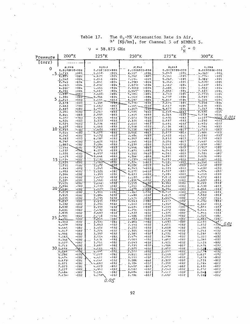
Table 17.
\)
The o2-MS"Attenuation Rate in Air, a' [Np/krn], for Channel 5 of NIMBUS
I 0 = 0 N
5.
Pressure
58.875 GHz
225°K [torr)
0 ALPHA O,OGOOOOO+OOO
ALP~A ALPHA O.POCSOOC+OOO C,COOGOOO+OOO
.5~- -oo5 e.Jt7 - -oo6 &.855 ~do5 -3-.-?-42 -=oos 1.542. -004 7,294, -oo5
z-;i4-1• -0 04 1. 29E t ·-o 04 4.2821 -004 2.025< ·-004
·E>.16£' -ao4 2.91H 8.391 -004 3.C)b'3~
1.09~ -::oo4 ~~-e<;;
5_1!386 -004 6.~&0;
-1LLLL----~~i-·--~~~-~--~-;0~0*3~--~5~·~-G~9~7~·----~~~--~~~ 2.C70 9,796• 2;·4&3 1.-1os• 2.88'.: 1,367•
3.350 '1:585-3.844 1.81'.:
-.--:3n ·2;c1o 4.934 2.336 -5-:52~ 2.-61e bo157 2,916
10 &:en 3:230 -7.514 3.56G -8:242 3 ;906 9.~03 4.2&7 9;797 4,645 1.062 5.~3e
l::"fi+e· nc-+----5~46-
1.237 5.871 1;330 -6~-31f
1.425 6,766'
15 T;: 24 ----:-ri'rlr ----;:...:...;~~-:::T.~-t-----,:,-7·-'-'; 2~-3;-;7-''--.::~IT---r.t26 7.724. T.7TI ~...,;,;<-+-- s • 2 2 E:-; 1.840 8.743. 1,951 -c,-;2-75· 2.06& 9.e23 z·;184. 1.c3e· 1-;s12 2.305 ~~-r--- 1.096 7.931 2o42'l 1,155 ~~~t--e:-361 z.ssE 1.21E e.eo2
20-z-;Tat'· 1-;27-g ~9-;254 2.€19 1.342 9.717 2;955 -1.408 1--;o1s 3.095 1,474 1.0&7
3:237' 1:54:3 :-; _-;o.;o"'2.t-----r:-fn 3.382 1.&12 ;-oo2 1.167 3. 5_3 c -1: 6 8 4 ;~ 0 2 -1 ... -2 1 9 3.681 1.756 -002 1.272 3;-8-35 1-.830 -~002 1.325
ALPHA 0.0000000 >JOO 4.345 1 -006
-1-:-734~ ·:ao5 3.901' -005 6.935~ -oos t.G83' -004 1.560: -004 2.123: -004
2:Tf3t ~oo-;;-3.5os· -oo4 4,331 .:oo4
---s:z41f--:.-lf04-6.236 -o·o4 7.317 -004 8.485 -004 9.738 -004 1.107~1 1.250 -003 1.401· ::.oo3 1.S&1 -003
- L-7-2"9· ::OOT 1o90f. -ryo3 2 • c 91' - 0 0 3-.2.285 -003 2.1.87 -003 2.&9e -oo3 ~7 ~03 3,145 -003 3.381 -003 3.626 -003
--~~t---___c;-3-=-· -:-B;--7 -;;-s - o o 3 · 1..140 -003
- ... 410 :;-!lOT 4,E 88 -003 4 • 9-7" -a ·o 3-5.26g -003 5 • 5 7 2 --0 0 3. 5.683 -003
6:202 =oD3 &.530 -003 6.-8-66 -003 7.210 -003 7·:5&2 -003 7,'!22 -003
T.29G -=oD3 5.6&7 -003 9-.t5i ~oo:3 9.444 -003 g,e44 -oo3
-002 25
]·.9_'!~ 1.90t -002 1.380 - T~-cf83 __ -.,..·~_,o,..,o,..,2:+-----7t--"-.--"-4--:::-3~E -----7~-+----7-"--::-::c.::-..;::....-"7::-2.061 :-oo2 1.493
5.34& 5 .527• 5. 711
30 s.ege &.08e
-&-:zao _&,4_74 b. 6 71• &.871 7. 073 7.277 -i-:~-9 4' 7. (941
2.141 -002 1.551 2.222 -002 1.610 -00<! 2,305 -002 1.E70 -002 2.38'l -002 1.731 -002 2.474 -002 1.794 -002
.? • 56 1 - 0 0 2_ 1 • 8 5 7 - 0 0 2 2o64'l -002 1o921 -002 2,739 -002 1.98& -002
3.514 3. f.J( 3. 761 3.887 4,G15 4,14S
~~1---~z~._,e~2~s, _____ -~o~o~2+---~2~·~o~52 -002 ~2_,_"l_22 -o o2 2 ,11-g------+~+----7-.!..;:-:;-~---o 02 4;?7.7 4.411 4o54f. 4.683 4.823
__ 4~9f>3 r; .1 or) 5,2'5P'\._
o.os
3,oE -=-o-o2 --2-;iaa -oo_2_ 3.110 -002 2.?57 1,678 -002 3.206 -002 2.327 1.731 -002 3,30~ -002 2.398 1.784. -002 3,40? -002 2.~10 1.aJe -oo2 3 • ~ 0 2 ~ 0 0 2_ -- _2 • s 4 3 1. 8 g 2 - 0 0 2
-3-:r.oi. -002 2.617 -ao2 1,94~ -002 3.706 -002 2.69? -002 2.001/ -002
92
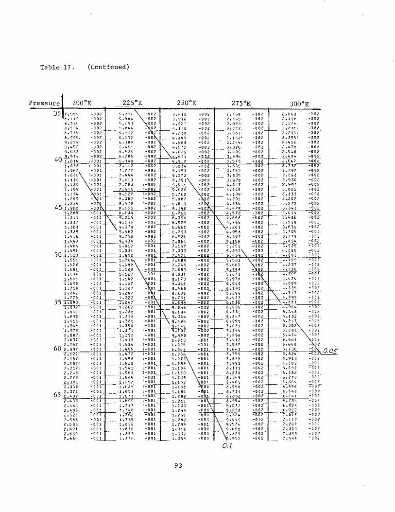
Table 17. (Continued)
Pressure 200°K 225°K 250°K 275°K 300°K
35 l.'JO~ -a o <' ~. J ~f 3. ~ 10 -002 ?,l&R 2.0b0 -002 A • 11 <: -002 IJ.'J44 J,<ll{, -002 2, R45• 2.11 e . -0 0 2 8. 3 Jt -002 ~'. t.g .1 4,C?~ -002 ;> ,<;2J• 2.1 7f->t ; - o a 2 R.~st. r,. e 4 4 -002 3. c 0 ;>' ?.?.1':1 · -o a 2 8, 7 7S· ':1. ':1 ') 7 J. 0 81' 2. 2 9S, -002 e. CJ9~; 6.1'>? 3.162~ 2. 3551 , -a o 2 9.2?4. b •. 3 0 p 3, 244 I 2 .4\t -002 g.45? 6 ,t.6r 3 .326· 2.478 .-a a 2 q,682 6,621) :S.40S -002
4Q_h"JIL, 3.494 -002 1.014 ·3 -:-s 1 g -: oi.lz-1.038 _, 3.665 2. 32 -0 0 2 -(~ Cf>2 :3.752 2.797 -002 l.t86 2.e63 -002 1.110 2.930 -002 1.135 2.997 -002 1.15'!
.. 3 :-o 65 ::-JoZ
1. 1 84 3.133 -002 f.2og 3 •. 2 a 2 -002 1.234 3.272 -a o 2
45"1.260 'j. 343 -002 1.285 3.414 -0 0 2 "1:-3i"l 3.48t ~002
1.337 3.558 -002 i~363 3.631 -a o 2-1.389 - _3_. 705 -0 0 2 1.416 3.77' -002 1.443 3.854 -002 T;46s --3~s-zs -=oo-2-1o49E 4.C05 -a o 2
50 1 :s23 4 :o82 -:aa2 1.S51 4.15S -002
-1; 5 7e 002 ·-4~237 -a 02 1,60E - 02 4. 31f: -002 1.634 -=-o 2 ~.-3gc; -=-aoT 1.661 -oo 4.474 -002 T~69-o :oo2 --4.555 ·002
-002 4.E:35 -Q02 :.o-o2 --4-.717 :.oo2 -002 4,79g -o o 2 -002 4,eeT -:ooz--002 4.%4 -002 ;:o o 2 5.048 :ooz -002 5.132 -0 0 2
1 • <J 1 ~I 6.959 =oo2 5.217 =~02 1. 948( ; -a a 1 7.t71 -002 5.302 -002
1:97-e: ;-:-o-oT T.ffi" -002 5;388 =-oo-z 2. 0 0 71 ,_a o 1 -001 7.298 -002 5.474 -002 2-;-o37~ '- 0 0 1 ,:_1 0 i -7-.412 --0 02- 5.561 002 2. 0 6 7; .-o a 1 : -o o 1 7.527 -002 5.648 - 02
60 2;097: ..: a a 1 :-o o i 7.643 ::-ooz 5,73E: -o 2 .127; - o a 1 1•001 7.75S -002 5.824 -002 2.157; -001 , -o o 1 7.8H -002 5o'l13 -002 2.1 R 7! -o 01 ) -0 0 1 7.993 6.002 -002 -~21 71 --0 01 ;:o-61 -e-; i l1 ~--- 6-·.· a·g2 -=o·a2-2. 248; •001 1. 563 1-0 01 _1)_._230 6.182 -oc2 2-:2?e1 -a o-1 -1.585 t-oo-t" 8,34g 6-.273 -002 2. 3 o~· -001 1,6Q7 '- 0 01 8.46S to3&4 -002
2.340: -:-o a 1 -r;-cz<F j~0-01 T.SiJo ~45[ -=-o oz ..
65 2. 371: ·-a o 1 ·1.651 t- 0 0 1 8.711 6.!'4e -002 2.4021 -ool 1. 67 3 8~ 832 6o641 -o o 2 2,4331 •001 1.6q'j 8.954 6. 734 ---002 2.464 -a a 1 1. 71 i g,U77 6.82P. -a a 2 2. 495· -001 1.740 q.2oo 6.922 -002
2".52f -~a a 1 "1:""?7;2 -... -.-321; -i-."0"17 -=-a·oz-2. 558 -a a 1 1.785 7.112 -002 2.58~ -001 1.eoe 7.207 -002 2.&21 -001 1.1\lO 7.30~ -002 2,£>r;2 -001 1.853 7.399 -002 2.664 ·001 1.8H. 7.4g6 -002
0.1
93
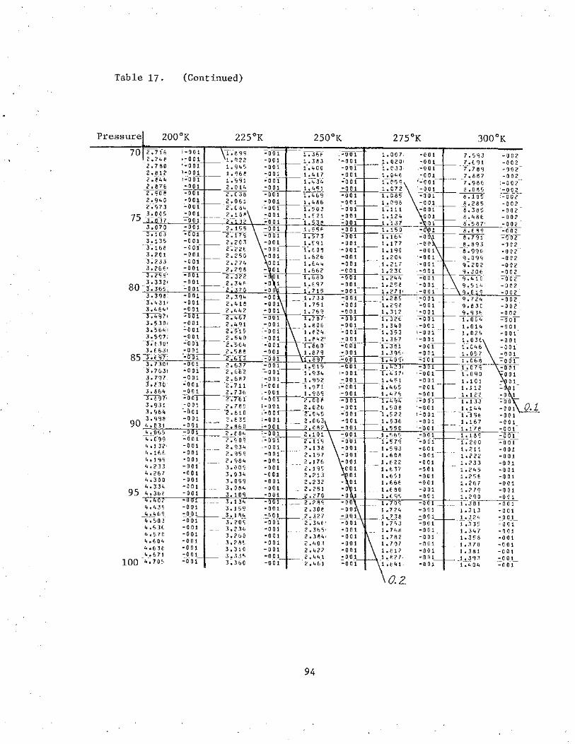
Table 17. (Continued)
Pressure 200°K 225°K 250°K 275°K 300°K 70 2:716 7. s gJ -002 2.74e 7.('31 -002 2. 780 -i; 789 -~02 2.812 7.887 -002 -2~T44 -7~-986 :-002--
2.876 e.085 ·-o o 2 2.~oe 8, 1 8 5- :-=ooz 2.'340 8.285 -002 2-;~73 '8. 385 -0 0 2
75 t~i; 8.48€: -002 -8---;-587• -002 3,070 8, E ~9 --ilOZ
3:103 8.7'31 -:-Q"oT 3-135 ·-0 p 8.8'33 -10 2 -·:r; u;e -f0-1 ·-a·. 9'36 -0 0 2--3.201 · -o o 1 g,ogc; -002 -3-;- 2 3 3 -1.£:44 :-o of '3~ 2 0 2 -002 3 .2&E• 1.662 --0 01 9.301: -002 3. 2<;9-1
1.680 -=--oo 1 9----;--410 -=-oc-2 80 -- 3 o332< 1,E'37 . -0 0 1 - 9.514 -002 3-;3&5: 1-. 715 . -0 0 1 '3 ~6 1 c; -002 3. 398: 1.733 :-0 01 9.724 -002 --3-; 431' 1.751 -;.001 9o83C -002 3 ,464' 1.7&'? '. 0 01 9.93~ -002 ~7'1 T;787· :-:-a 0 1 --r;o"G<.- -o-61
3. 5301 1.806 . -o o 1 1.014 -001 3;'5£,41 1. (24. 1- o or- 1~ 025 -001 3.597: 2.540 1, p 42' '- 0 01 1.03E -001 ---:f;tJO! -2 ;-5-&11 1.8&o-- ;.001- {;G46 -001 3. E&JI 2.?se 1.879 -001 1.057 -001 85 3,E97: z-.-&T3 -r-;-8-q? -:;001 ~8 -:-aoT 3. 730' 1 T;-ors -o o1 '3~7631 ,;.·o o 1 1--; 090 001 3. 797. -001 1. 1 0 1 - 01 -3~no· -o o i -i~-112 -
1 3.864 -001 1.122 -0 1 3~'1· ;-:-00-1 1~TD- ·=oo 3.931 ·-o o 1 1.144 -001 j,Cj6l, ~-.:-o o 1 'T;-15!: -001
90 3.998 2. e 3~ '- 0 01 1.107 -001 4. 0 31 2.860 ·-ooc f.178 -001 4. 06?· 2.e84 -001 1.18'? ::ooT" 4:c9<i -?-;s·aCJ -f:57~ .-_ o o-i 1-:2'00 ::OoT 4 ,j 32· 2.934 1.593 -001 1.211 -001 4-166 2.95'? 1.608 -001 1.222 -001
?.984 1.E22 -001 1. "3 3 -001 J.ooc; 2.195 1. ~37 -001 1.245 -0 01 3,034 2.213 1.6~1 -001 1o25E -001 3.059 2.232 1,66E -001 1.267 -001 3,084 2.251 -- 1.680 -001 1o?79 -0 0 1 95 3.109 2.270 -001 1.290 -001 3,134 2.?~c; -001 1 • 3 0 1 -001 3.1~9 2,3oe -001 1.313 ·001
_'!__!_~6c; 3,1R4 2.327 -001 __!_,__:J_ 2 4 -001 t..~03 -3-:-zo-s -T:34f' -=o1J1 1 .3 35 :.:-o01 4.53(; 3,234 2. 365• -001 1.347 -001 4o570 3,?60 2.3 84• -001 1o30.8 -001 4.604 3.<8~ 2. ,, 0 ,J' -001 1.~70 -0 0 1 4o63e 3.310 2.42? •001 I .381 -001
- 4,£,71 3,3.15 - 2.441 -0 0 1 _1_.__~93 -001 100 ~-; 7 05 3:3 60 2,461 -001 1.~04 -.=-o 01-
o.z
94

0.4 E a. a.
z <]
5 0.2 "iii ... Cl.l a. Ill
0
0
E ~ 2 ' Ill ~
\0 tl VI c
.5! 0 :::1 c
~ <X
00
Figure 32.
0.6
0.4
0.2 Dry Air
300°K
/:::,.11 = 25 MHz
0.2
0.1
0 IE':':. .c .. q I
OL-----------------------~
4
2
400 600 800 ° 0 200
Computer plots of o2-Ms continuum 58.8 GHz (±0.1 GHz).
Linear Theory , I~ = 0
400 Pressure, torr
THEORY
600 800
10
5
200 400 600
pressure profiles in AIR at 52.8 GHz, 54.9 GHz, and
800

2.6 Atmospheric o2-Ms Properties (40-140 GHz)
The transfer function of a homogeneous atmosphere is characterized
by the complex refractivity N = N' - jN" that has been treated in
depth for the o2-Ms in terms of dispersion ~N[ppm] and attenuation a
[dB/km]. A turbulent atmosphere introduces random contributions to the
refractivity N. Turbulence can be expressed by statistics of tempera-
ture and pressure fields; thus, a general transfer function calls for
the evaluation of temperature and pressure sensitivities (Ott, 1975),
a = 'da/'dTa T
a p
'da/'dpa
'd(~N)/'dT~N
'd(~N)/'dp~N (60)
[%/torr]
across the o2-Ms band (Fig. 25). A "modulation" of turbulence-induced
signal fluctuations occurs when the sensitivities a T,p and b T,p
depend upon frequency. A broadband signal (several GHz) can experience
decorrelation or, in other words, the turbulent atmosphere may exhibit
an ultimate bandwidth.
The frequency dependence of a b can reveal information T,p' T,p
about the state of the atmosphere via a differential measurement of
amplitude and/or phase of a (coherent) signal pair at selected frequen-
cies. Peckham (1974) proposes to measure with a satellite-based radar the
ground-reflected signal strength at several frequencies located in the
low frequency wing of the o2-Ms. If no precipitation is present, the
differential signal strengths are expected to be indicative of atmospheric
ground level (mainly over oceans) pressure. Wykes (1974) reported the
supporting calculations of 02-MS transfer characteristics between
47 and 54 GHz.
96
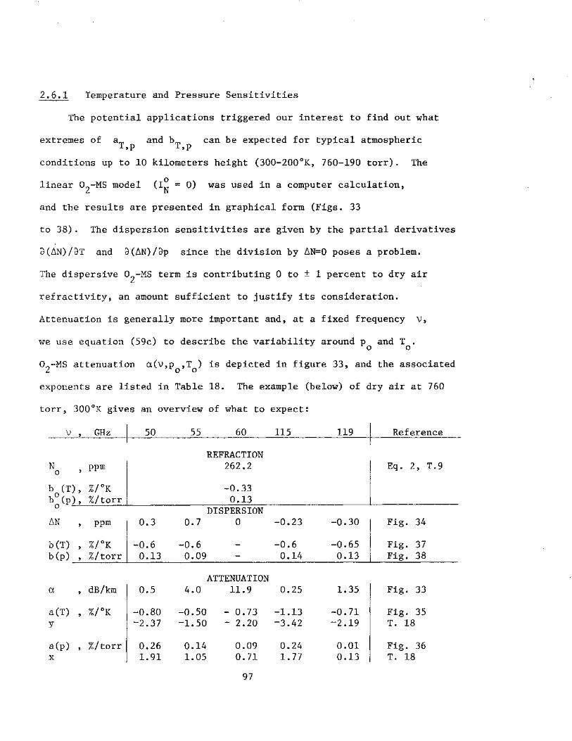
2.6.1 Temperature and Pressure Sensitivities
The potential applications triggered our interest to find out what
extremes of a and bT T,p ,p can be expected for typical atmospheric
conditions up to 10 kilometers height (300-200°K, 760-190 torr). The
linear o2-Ms model (I~ = 0) was used in a computer calculation,
and the results are presented in graphical form (Figs. 33
to 38). The dispersion sensitivities are given by the partial derivatives
a(6N)/dT and a(6N)/ap since the division by 6N=O poses a problem.
The dispersive o2
-Ms term is contributing 0 to ± 1 percent to dry air
refractivity, an amount sufficient to justify its consideration.
Attenuation is generally more important and, at a fixed frequency v,
we use equation (59c) to describe the variability around p and T . 0 0
o2-Ms attenuation a(V,p ,T ) is depicted in figure 33, and the associated 0 0
exponents are listed in Table 18. The example (below) of dry air at 760
torr, 300°K gives an overview of what to expect:
v , GHz 50 55 60 115 119 Reference
REFRACTION N ppm 262.2
0 Eq. 2, T. 9
b (T), %/oK -0.33 0 %/torr 0.13 b 0 (p) ,
DISPERSION 6N ppm 0.3 0.7 0 -0.23 -0.30 Fig. 34
b(T) %/oK -0.6 -0.6 -0.6 -0.65 Fig. 37 b(p) %/torr 0.13 0.09 0.14 0.13 Fig. 38
ATTENUATION a , dB/km 0.5 4.0 11.9 0.25 1.35 Fig. 33
a(T) %/oK -0.80 -0.50 - 0.73 -1.13 -0.71 Fig. 35 y -2.37 -1.50 - 2.20 -3.42 -2.19 T. 18
a(p) ' %/torr 0.26 0.14 0.09 0.24 0.01 Fig. 36 X 1.91 1.05 0. 71 1.77 0.13 T. 18
97

•
] 1.4
1 - 760 - torr ~ 12 T 300°K '"d 1.2 2 - 570
(j 10
3 380 1.0
~ 8 1- 4 - 190 •M <G 0.!1
l=l 6 •M
~
~t ~~ 0 4 •M -IJ t1l ;::l
2 l=l Q) -IJ -IJ <G 0
Ul I I I ::<:: I I I I I I I I I 4!1 !50 &tl eo 8& 70 16 10 10& 110 11& 120 12& 130 1M N
0 Frequency \) GHz
0 -MS 2 BAND 1-- Line
Linear Theory '
Io N
0
] 30 -~ T = '"d 2&
(j
~ 'M <G
l=l ·M
l=l 0
•M -IJ t1l 5 ;::l l=l Q) -IJ -IJ 0 <G Ul ::<:: I I 4!1 N
0
Figure 33.
3.&
200°K 1 - 760 torr 3.0 - 570 2.5 380
2.0 - 190
1.5
4 1.0
0.5
0
I I I I I I I I I I I I !50 &II eo 8& 70 16 10 10& 110 115 120 12& 130 1!6
Frequency \) '
GHz
Dry AIR attenuation due to the o2
-Ms at 300° and 200°K for four pressure parameters (190-760 torr).
98
j 140
140
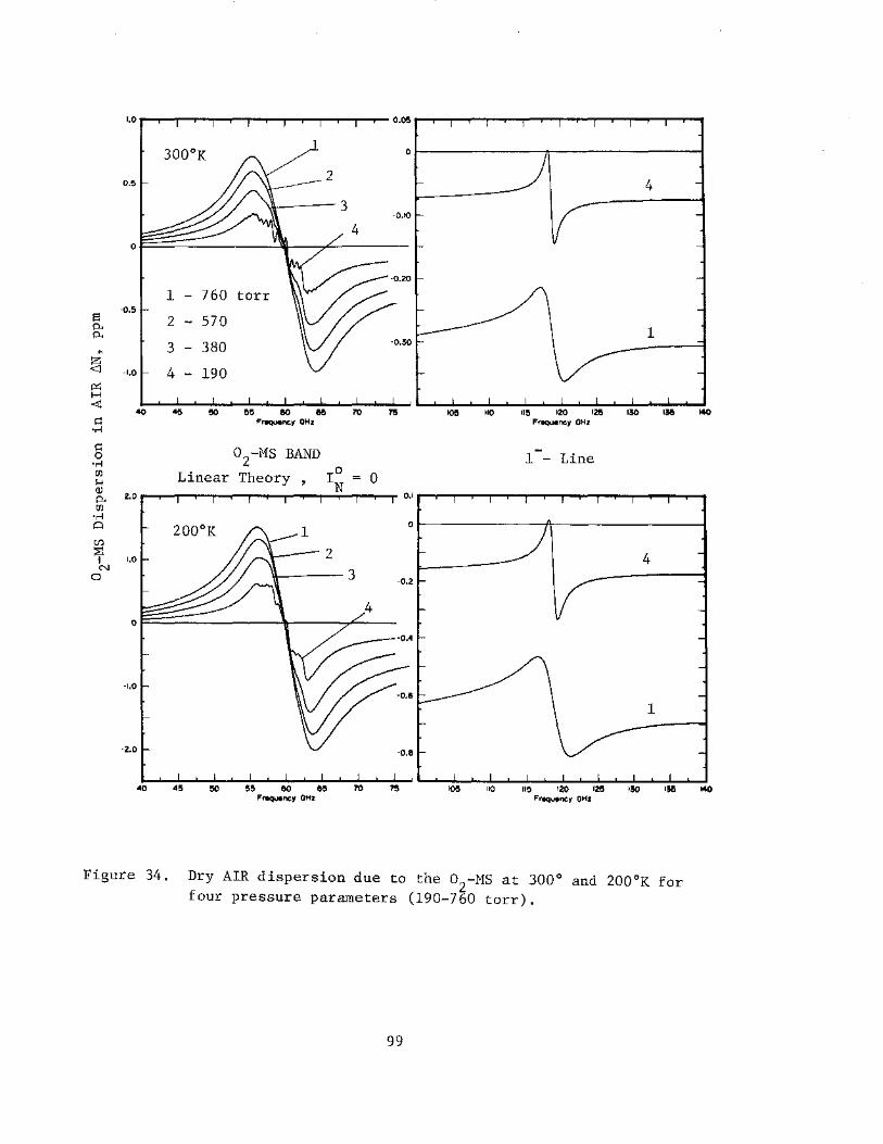
0~--------------~-----------------;
0.5
0
1 - 760 torr ·0.5
2 - 570
3 - 380
4 - 190
40
1-- Line o2-Ms BAND
Linear Theory , r; = 0 2.0 .-...-_,.--....--.-.--or-..,....._,.......,.....,......:;.:--r-..,...-r 0.1 .-...... _,.......,.__,.-.--.,.-..,...-r-..,.--r-.,...--r-..,..."'"T"...,.....,
40 115 120 125 130 138 Frequency OHZ
Figure 34. Dry AIR dispersion due to the o2
-Ms at 300° and 200°K for four pressure parameters (190-760 torr).
99

lf -0.6
.... QJ p.
E-. -0.8 <11
"' '-' ..... :> ..... ..,
..... ·1.0 Ul
" QJ {j)
QJ ....
" u
"' .... QJ p. s QJ E-
-1.2
40
o2-Ms Attenuation
760 torr
115
Frequency V , GHz
Figure 35. Temperature sensitivity aT = aa/aTa of o2
-Ms attenuation (see Fig. 33) at 760, 380, and 190 torr for three temperature parameters (200-300°K).
100
130

"' 0
H
"' P..
~ 0.6
~. w
·.-< >
·.-< w
·.-< (})
c "' U1
"' H :J w
"' H
"' n. 8
"' [-<
"' 0
H
"' n. ... [-<
"' ,.., w
·.-< >
·.-< w ·.-< <Jl c <lJ
(fJ
"' H ::l w
"' H (\)
P.. 13 <lJ
[-<
0.8
·1.0
·1.2
1.4
40
0
·0.2
·0.4
·0.6
·0.8
·1.0
·1.2
-1.4
40
45 50
45 50
0.6
200°K -
JKO torr )
55 60 65 7'0 1"5 ·00 'I(' •20 '25 ~[.
FrL'CJUt>ncv 'V , Cll?.
55 60 65 7'0 75 ·OC ·o ·zc
101

1-1 1.2 1-1 o2-Ms Attenuation 0 190 torr .w
1-1 1.0 Q) p..
iN!
0.8
p.. 111
:>. .w 0.6
380 ...... :> ...... .w ......
0.4 (f) 570 r::: Q) 760 Cl)
Q) 0.2 1-1
;; (f) T = 200°K (f) Q) 1-1 0 p..
40 45 50 55 85 110 115 120 125 130
1.2 1-1 1-1 190 torr o2-Ms Attenuation 0 .w
1-1 1.0 Q) p..
iN! <..8
p.. 111
:>. 0.6 .w 380 ·.-t :>
·.-t .w 570 ·.-1 0.4 (f)
r::: 760 Q) Cl)
Q) 0.2 1-1 ;; T= 250°K (f) (f) Q)
0 1-1 {:4
I I I I 40 45 50 55 60 85 '1'0 130
Frequency ll, GHz
102

~ 1.0 p..
ftp.. 0.8
<1l
:>. .u ·r-f :>
·r-f .u ·r-f UJ s:: Q)
Ul
Figure 36.
190 torr
380
570 760
40 45
GHz
insensitive to p
Pressure sensitivity a = Cla/Clpa of o2-Hs attenuation (see
Fig. 33) at 200, 250, aRd 300°K for four parameters (190-760 torr).
103
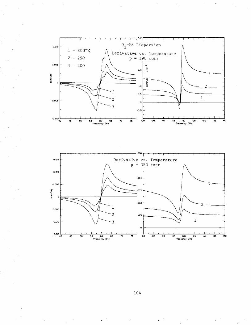
0.010
1 300°1{
2 - 250
0.005 3 200
\__2 l e 0.
0 0.
1 2 ·0.005
3
-0.01040 45 50 100 10!1 110 130
·.006
0.015 Derivative vs. Temperature p = 380 torr
0.010
.004
•.OOil-_______ ~
-0.010
45 60 G5 55 F,.quenc:y OHz
100
104
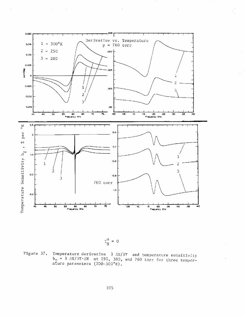
0.020
f Q Q
40
~ 0.!5 0
H Q) 0 0.
~
E-< ,.0
>-. +J •r-l :>
•r-l +J •r-l
CIJ (:1 Q)
C/)
Q)
H ;:j +J t1l H Q)
.009
vs. 1 - 300°K p 760 2 - 250 '.007
3 - 200
.005
.003
4!5 !50
·0.6 ~---------.---------
760 torr
0. 40 4!5 13 Q)
E-<
Temperature torr
110 11!5 120 12!1 Frequency OHz
Figure 37. Temperature derivative a 6N/8T and temperature sensitivity bT = a 6N/8T·6N at 190, 380, and 760 torr for three temperature parameters (200-300°K).
105
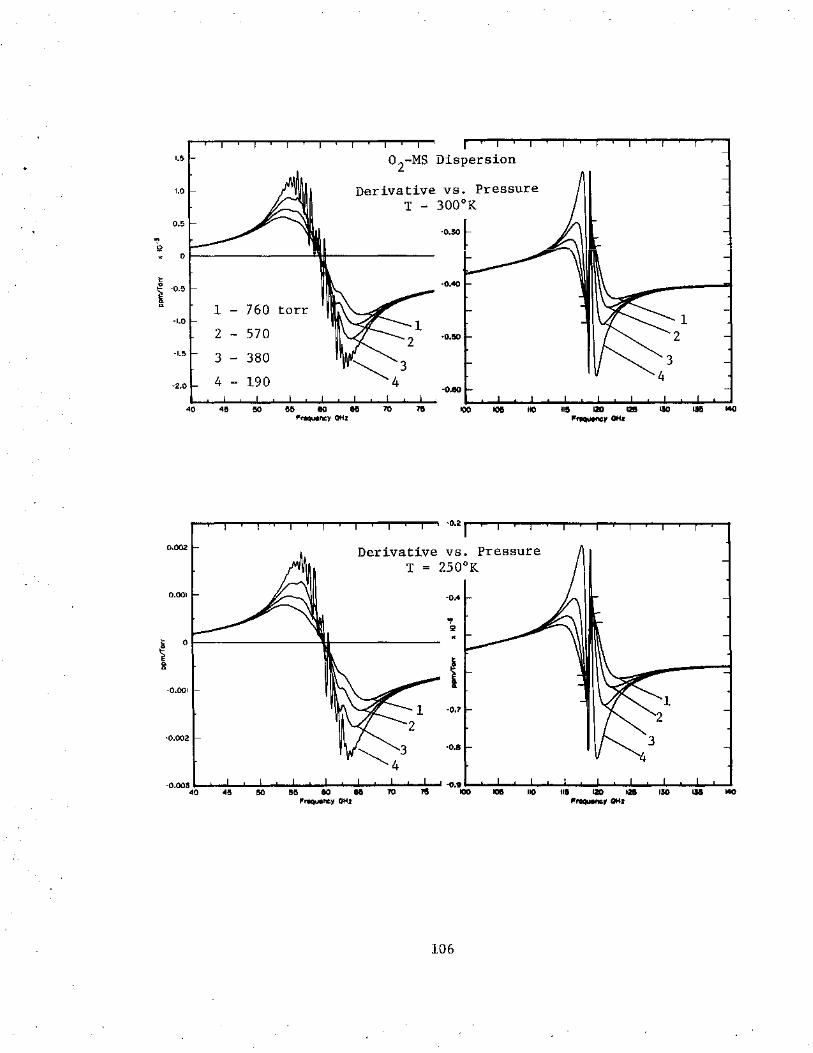
1.5
1.0
0.5
., Q
0
t -0.5
D.
40
0.002
-0.001
-0.002
1 - 760 torr
2 - 570
3 - 380
4 190
o2-Ms Dispersion
Derivative vs. Pressure T - 300°K
-0.40
-0.!10
-o.eo
!10 55 eo e Frequency OHz
Derivative vs. Pressure T = 250°K
-0.4
.. 2
i -0.7
-o.e
106
140
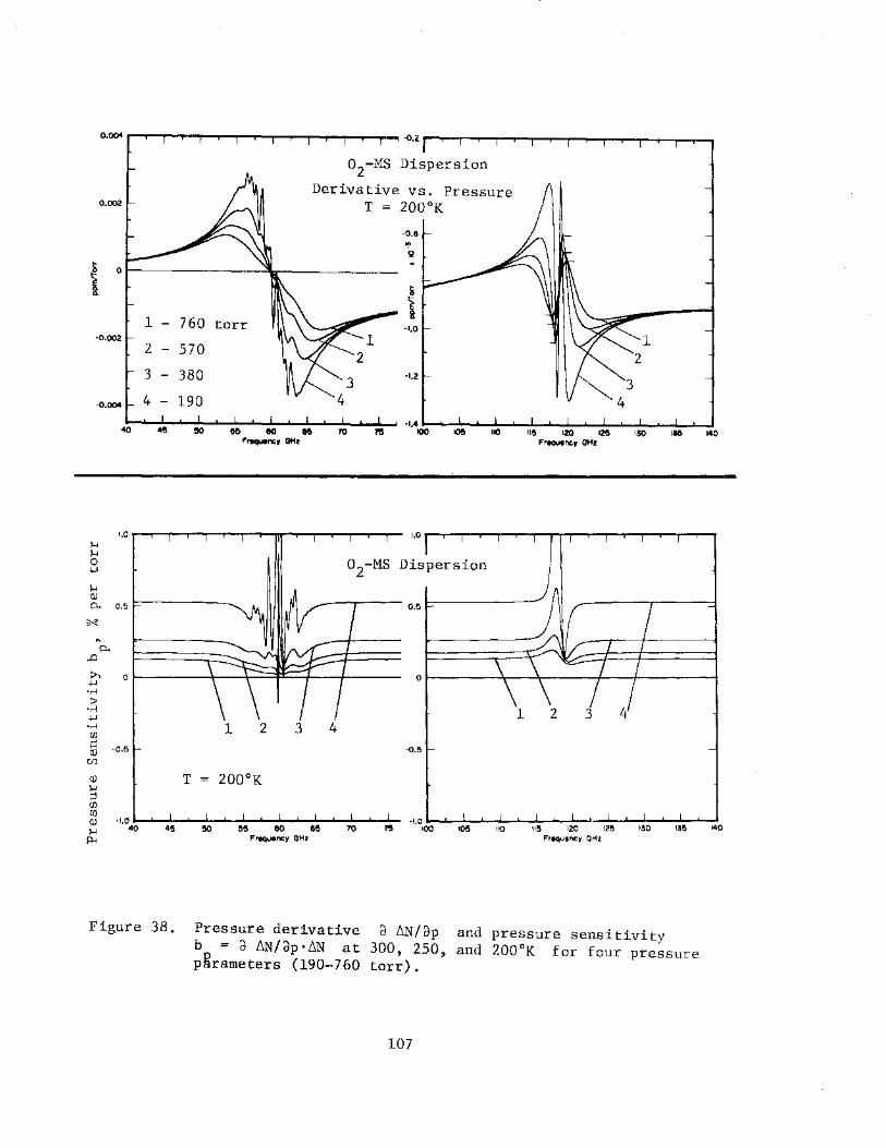
0.002
1.0 l-1 l-1 0 .j.J
l-1 <ll p.. 0.5
iN1
" p.. ,.c
:>-. 0 .j.J
•r-i :>
•r-i .j.J
•r-i UJ (:!
-0.5 <ll U)
<ll l-1 ;j UJ UJ <ll ~t.O
l-1 40 p.,
1 - 760 torr
2 - 570
380
190
1 2
T 200°K
3
o2-Ms Dispersion
Derivative vs. Pressure T = 200°K
0 -MS 2
4
·0.8
"' 2
1.0
0.5
·0.5
·1.0 100 10!1 110
1
II!! Frequency OHz
Figure 38. Pressure derivative b = a ~N/op·~N at pRrameters (190-760
a ~N/ap 300, 250, torr).
and pressure sensitivity and 200°K for four pressure
107
140

Table 18. Pressure exponents x and temperature exponents y of the o2-Ms attenuation
( a for two pressure (760, 570 torr)
0 ) and two temperature 300, 200 K parameters X -y
Freq. 760 torr 570 torr 760 torr 570 torr I Po v 300°K 200°K 300°K 200°K 300°K 200°K 300°K 200°KI To
GHz 40 1. 99 1.98 2.00 1. 99 2.79 2.81
I 2.79 2.82
45 1.98 1.96 1. 99 1.98 2. 71 2.76 2.72 2.78 50 1.91 1.88 1.94 1. 93 2.37 2.59 2.36 2.62 51 1.84 1.84 1.88 1.90 2.17 2.50 2.12 2.53 52 1. 72 1. 76 1. 76 1. 84 1. 91 2.37 1. 79 2.39 53 1.53 1.63 1.57 1. 73 1. 66 2.19 1.47 2.19 54 1.30 1.44 1. 33 1.54 1.51 1.98 1.32 1. 93 55 1. 05 1.18 1.09 1.26 1.50 1.79 1. 37 1. 72 56 0.85 0.93 0.87 0.97 1. 61 1.69 1.55 1.62 57 0.78 0.75 0.83 0.82 1. 82 1.71 1.84 1. 72 58 0.73 0.61 0.78 0.68 2.03 1.77 2.11 1.85 59 0. 72 0.54 0.80 0.63 2.18 1.83 2.30 1. 97 60 0. 71 0.52 0. 78 0.60 2.20 1.83 2.32 1. 97 61 0. 72 0.56 0.80 0.66 2.11 1. 79 2.21 1. 91 62 o. 71 0.63 0.76 0.70 1.90 1.71 1.95 1. 76 63 0.76 0.78 0.80 0.83 1. 70 1. 68 1. 70 1.66 64 1.00 1. 07 1.05 1.18 1.59 1. 79 1.50 1. 75 65 1.23 1.36 1. 26 1.47 1.55 1.97 1.37 1. 92 66 1.47 1.58 1.50 1.69 1.64 2.16 1. 44 2.14 67 1. 67 1. 73 1.71 1.82 1.85 2.34 1. 70 2.36 68 1.81 1.82 1.85 1.88 2.11 2.48 2.03 2.51 69 1.89 1.87 1.92 1. 92 2.33 2.58 2.30 2.61 70 1. 93 1.90 1.96 1.94 2.48 2.64 2.48 2.67 75 1.98 1. 96 1. 99 1.98 2.74 2.78 2.74 2.79 80 1. 99 1.98 2.00 1. 99 2.80 2.82 2.81 2.83
100 2.00 1.99 2.00 2.00 2.92 2.95 2.92 2.95 110 1. 98 1.94 1.99 1.97 3.18 3.25 3.19 3.27 112 1. 95 1.88 1.97 1. 93 3.30 3.33 3.32 3.39 114 1.87 1. 73 1.92 1.83 3.41 3.36 3.46 3.46 115 1.77 1.57 1.86 1.72 3.42 3.29 3.51 3.44 116 1.58 1.30 1. 73 1.51 3.34 3.12 3.49 3.32 117 1.18 0.86 1.41 1.09 3.05 2.78 3.28 3.01 118 0.45 0.31 0.61 0.39 2.46 2.32 2.62 2.42 119 0.13 0.14 0.13 0.11 2.19 2.17 2.21 2.17 120 0.84 0.57 1.09 0.76 2.79 2.54 3.02 2.73 121 1. 40 1.09 1.60 1.33 3.24 2.97 3.43 3.20 122 1. 68 1. 43 1.80 1.62 3.42 3.23 3.54 3.42 123 1.81 1. 64 1.89 1.77 3.46 3.36 3.54 3.50 124 1.88 1. 76 1. 93 1.85 3.46 3.42 3.51 3.51 125 1. 92 1. 84 1. 96 1. 90 3.43 3.43 3.46 3.50 126 1.95 1.88 1.97 1. 93 3.39 3.42 3.41 3.47 128 1. 97 1. 94 1. 99 1. 96 3.30 3.37 3.32 3.40 130 1. 99 1. 96 1.99 1.98 3.23 3.31 3.24 3.33 140 2.00 1. 99 2.00 2.00 3.05 3.11 3.05 3.11
108

Scanning Table 18 for decorrelations of pressure and temperature
sensitivities, only the 1- line center attenuation at 119 GHz proves to
be fairly insensitive to pressure variations (x 0.13), hence the
strength of a radio signal at this frequency is a good indicator of
integrated temperature fluctuations along a line-of-sight path (y = -2.2).
Picking o2-Ms attenuation as a pressure indicator seems to be a poor
choice since the variability with temperature dominates at ground levels
for all frequencies. The variation of both exponents, x and y, with the
mean pressure or mean temperature is relatively small compared to the
changes with frequency (Table 18). The value of o2-Ms dispersion (Figs.
34, 37, and 38) to sensing the state of the atmosphere was discussed
briefly in Section 3.1.2 of Part 1.
The results of figures 33 to 38 depend upon the line shape and
width (e.g., Wykes, 1974) and they will be slightly different for the
"Overlap" model (I~- Table 1).
3. WATER VAPOR STUDIES
Water vapor exhibits a rich rotational spectrum of which two lines
appear below 200 GHz. The influence of water vapor upon microwave
transfer characteristics can be analyzed by (Eqs. 1 to 3)
aw = 0.1820V[(SF")l + (SF")z + q"]
L'IN w
(SF') 1 + (SF')z + q'
[dB/km],
[ppm] •
The terms (SF)l,2 16 identify the two H20 microwave lines, and
(61)
q = q' - jq" all contributions in excess of these two lines. A few
remarks are made regarding difficulties encountered when studying a and w
L'IN either in the laboratory or the free atmosphere. All results, w
especially anomalies that are discussed in section 3.2, should be judged
in light of these remarks. 109

Water vapor is a difficult test gas inside a vacuum vessel since it
strongly adsorbs upon all surfaces. The exchange process with the wall is
reversible for isothermic conditions, but the time period to reach equilib-
rium is in the order of 0.5 to 5 hours depending upon T and how close
is to saturation (Liebe, P-8). No sure means have been found to eliminate
adsorption. Mrowinski (P-9) experimented with Teflon coatings but only with
partial success. Forming water layers alter homogeneous gas conditions and
the detection capability of the resonance spectrometer.
Water vapor in the free atmosphere is known to vary considerably, both
in time and space, making point measurements of pw highly unreliable to
represent the moisture content along a radio path.
3.1 Water Vapor Microwave Line Spectrum
The two microwave H2o lines are centered at 22.2 and 183.3 GHz. Their
strengths are given by (Sect. 2.5 - Part 1)
S = (v!vJ s~, 2 (300/T) 3 • 5 pw exp[w1 , 2(1-3~0)]
The line parameters at 300°K are
Line 1
(62)
2
V - center frequency 0
22.23515 183.31012 GHz
So - h strengt parameter
w - temperature exponent
0 Y - width parameter
w
13.9 322 Hz/torr
2.14 0.653
18.0 19 MHz/torr .
The line shape in moist air that fitted laboratory data (Becker and Autler,
1946) best, was the Van Vleck-Weisskopf shape, which follows from equations
(5), (6) when assuming I0
= 0. The linewidth is
y = y0 [0.21 (300/T) 0 •6 p + (300/T)p ] w w w [MHz], (63)
whereby p is the dry air pressure in torr. The formulation, so far, does
110

not yield correct answers for a and w
Lm w
since the nonresonant term q
needs to be added.
3.2 Nonresonant Water Vapor Microwave Spectrum
A nonresonant excess q1 is expected from the far wings of all higher
frequency lines. It is a weakness of the Van Vleck-Weisskopf shape that it
does not describe the intensity distribution in the far wing (~lOy). For
this reason one tends to adapt the Gross shape (Liebe, 1969),
F" 2 2 2 2 4v2y2] 4v y/ [ (v - v ) + and G 0 (64)
2v (v 2 - v2)/[(v2 2)2 4v2y2] F' - v + ' G 0 0 0
for calculations of the H2o spectrum between 1 and 1500 GHz since it predicts
higher intensities in the low frequency wings (Hall, 1970). The wing
contribution is expected to be proportional to the pressure p • w
Laboratory attenuation data taken between 18 and 42 GHz at p ~ 760 torr
and p = 0 to 50 torr were fitted when w
[dB/km] , (65)
which is about five times as large if the Van Vleck-Weisskopf shape is used
for the wing contributions of all higher frequency lines (Becker and Autler,
1946). Similar high wing attenuation was measured for H2o and H20+N2
mixtures between 120 and 300 GHz (Frenkel and Wood, 1966).
Deviations from a pressure-linear dependence of q lead to the intra-
duction of a second contribution proportional to 2 p .
w Such quadratic term
2 q2 (pw) presents evidence of pressure-induced (involving pairs of H2o
molecules) polarization effects, which can occur from a spectrum of a dimer
H200H2 (e.g., Braun, P-15; Dyke and Muenter, 1974) and/or as a consequence
of quenching of the rotational motion of the H2o molecule by intermolecular
forces. Indications of nonlinear behavior of a (~N ) with respect to pw w w
111

exist from a variety of experimental studies:
(i) Line-of-sight radio path attenuation
(70 and 79 GHz - Hogg, 1971; 179 and 184 GHz - Whaley, P-5;
222 GHz- Malyshenko, 1969).
(ii) Zenith path attenuation
(36 GHz- Hogg, 1971; 80 to 130 GHz- Gibbins et al., 1975).
(iii) Spectroscopic absorption and dispersion
(22 GHz- Mrowinski, 1970; 119 GHz- Tolbert et al., 1964;
184 GHz- Hemmi and Straiton, 1969; 225 GHz- Harries et al.,
1969; 22.2 and 23.6 GHz- Dillon and Liebe, 1971).
We report some a and w ~N measurements with the PRS at frequencies
w
between 22.2 and 61.2 GHz using pure water vapor. Extreme temperature
control (< ± O.Ol°K) throughout the system was essential to approach
saturation pressures in a reproducible manner. Water vapor generation in
a double-walled hard-glass bulb and inlet tubing, where the jacket was part
of the temperature circulator flow, enabled to reach 99 percent saturation
as checked with an integrated dew point hygrometer.
Results of the types shown in figures 39b, 40, and 41 are roughly
described by
where V is the frequency in gigahertz.
The theory of (H2o) 2 dimer microwave attenuation was treated in some
detail by Poon (1974). His theoretical findings can be expressed as
112

a . ~0.2 2 (v/60) 2 "4 (300/T) 16 ·10-3 D1mer pw [dB/km] (68)
Noteworthy are certain similarities between equations (67) and (68) in
respect to a strong temperature and some frequency dependencies. An
Arrhenius plot (Harries et al., 1969) of a at 61.2 GHz (Fig. 40) w
yields as gradient of constant pressure data the value 4.5 kcal/mole.
The same procedure of the dispersion data delivers 8.5 kcal/mole. We
believe that dispersion pressure profiles are erroneous due to surface
adsorption effects while attenuation profiles are much less affected.
More evidence of anomalous water vapor polarization is given in figures
39c, and d. The deviations from equation (2) in figure 39d are attributed
to the real gas law (van der Waals equation), which relates pw to the
number of molecules per unit volume,
M ~ 9.66•1018 p /(T - pwB2/62366) 3 (69) [1/cm ] w
The second virial coefficient 3 B2 [cm /mole] is discussed by Bohlander
and Gebbie (1975).
All data are only sketchy evidence of anomalies in the microwave
spectrum of water vapor, which warrant more systematic studies of a and w
~N over a wider range of temperatures, frequencies, and close to w
saturation. At present, there is no satisfactory theory to account
for the experimentally observed excess q.
113
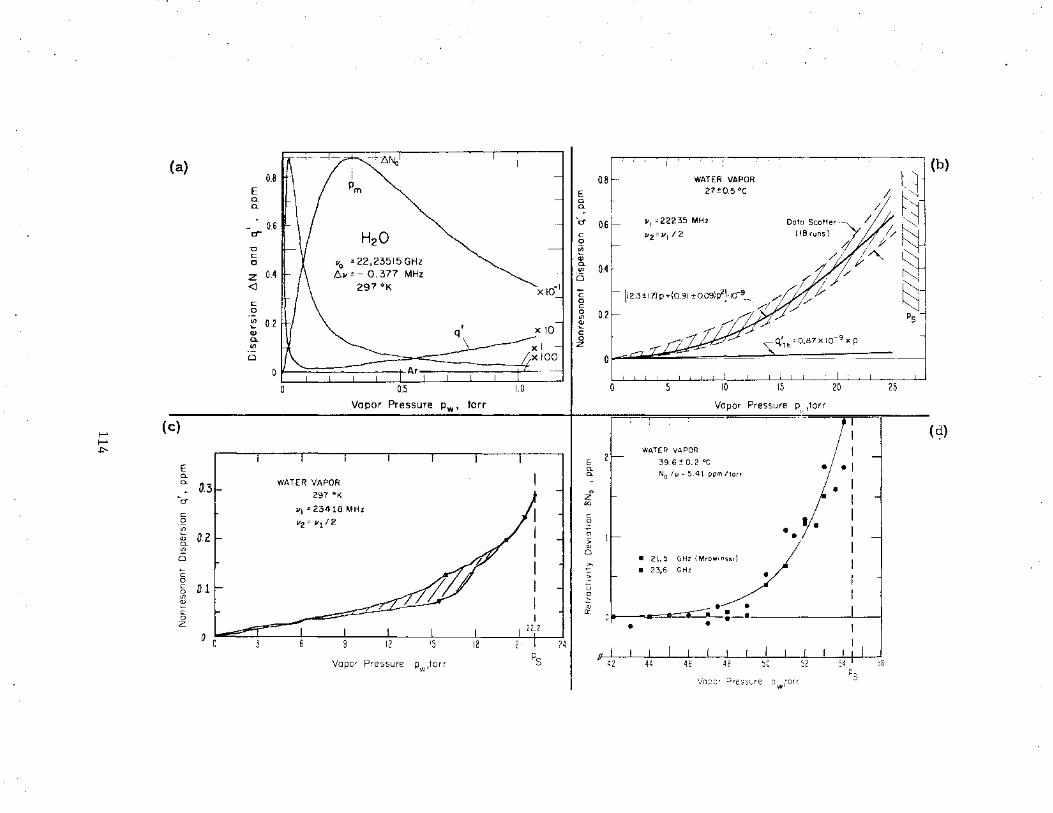
1-' 1-' +:-
(a) o.a E 0. 0.
• 0.6 -~
"0 c: 0
z 0.4 <l
c: 0
~ 0.2 (1)
0.
"'
H20
110 =22,23515GHz 611 =- 0. 377 MHz
297 °K
0 0~
(c)
E c. c.
·r:r c: 0
'jjj
~ 0.2 V>
0 c: 0
§ 0.1 V> Q.l ~
c: 0 z
0 0.5
Vo por Pressure Pw, torr
WATER VAPOR 297 °K
111 = 23418 MHz
112 =111 12
1.0
I -'· I I .'.. •" I "' --~~r:=---~r-'------0...._....--! A
0
Vapor Pressure pw,torr Ps
II t4
E c c. .
-ct
c: 0 jjj
~ c. V>
i:5
c 0 c: 0 V>
~ c: 0 z
E a. a.
0 z "' c: 0
0 > "' 0
'"' =: u ~ o; 0::
0
l 0
WATER VAPOR 27!0.5 •c
Ill •22235 MHZ
11z=11112
[(2.3±1.7)p+(0.91 ±0.09)p2]·10_9_ /1 ''//
15
Dote• Scoller (18 runs)
Vapor Pressure
•
WATER VAPOR
39.6±0.2 oc; N0 /p = 5.41 ppm/torr
• 21.5 • 23,6
a,.
11 I 1 1 I 1 1 1 r I r 42 44 46 48 50
Vapor Pressure pw1torr
t J /, -~
/~ t~i ~~~ /1 I?;/
J-"'-
56
(b)
(~)
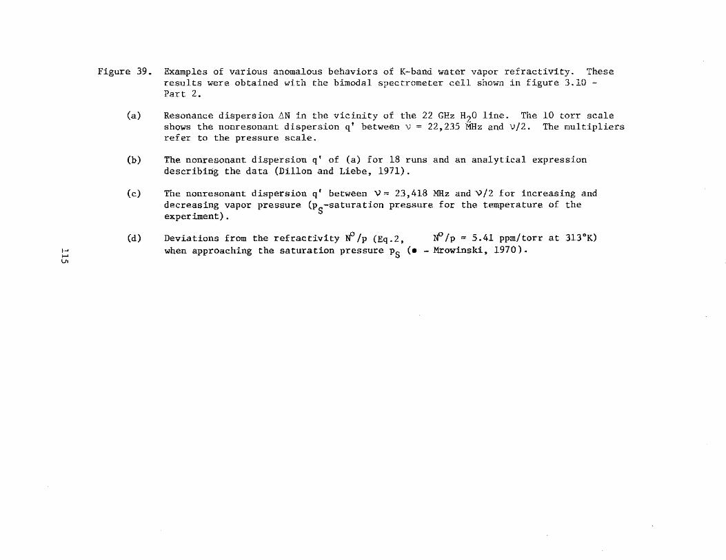
I-' I-' V1
Figure 39. Examples of various anomalous behaviors of K-band water vapor refractivity. These results were obtained with the bimodal spectrometer cell shown in figure 3.10 -Part 2.
(a) Resonance dispersion 6N in the vicinity of the 22 GHz H20 line. The 10 torr scale shows the nonresonan~ dispersion q' between v = 22,235 MHz and V/2. The multipliers refer to the pressure scale.
(b) The nonresonant dispersion q' of (a) for 18 runs and an analytical expression describing the data (Dillon and Liebe, 1971).
(c) The nonresonant dispersion q' between V= 23,418 MHz and V/2 for increasing and decreasing vapor pressure (p
5-saturation pressure for the temperature of the
experiment).
(d) Deviations from the refractivity Nf/p (Eq.2, Nf/p = 5.41 ppm/torr at 313°K) when approaching the saturation pressure Ps (• - Mrowinski, 1970).
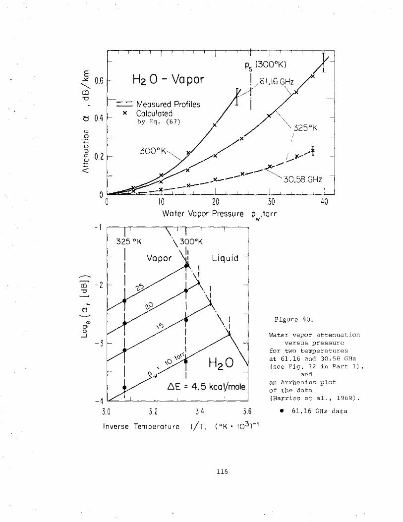
E p
5 (300°K)
< 0.6 H2 0- Vapor ! 61.16GHz/
i/ ro "0
?j
c 0 -0 :::J c (l) --<!
-,........., co "0
.... tj ...__....
Q)
C'l 0 _j
0.4 -
0.2
00
-1
-2
-3
=-= Measured Profiles x Calculated
X / ~325°K
/
x I
by Eq. (67)
300°K M / /IVA / x ........ ~
./~ X_...-~ x~ __ x-_.- 30.58 GHz -_x-10 20 30 40 Water Vapor Pressure p ,torr
w
\ 300°K . II
Vapor • Liquid
I ~E = 4.5 kcol/mole
Figure 40.
Water vapor attenuation versus pressure
for two temperatures at 61.16 and 30.58 GHz (see Fig. 12 in Part 1),
and an Arrhenius plot of the data
-4~--~--~--~~--~--~--~ (Harries et al., 1969).
3.0 3.2 3.4 3.6 • 61.16 GHz data
Inverse Temperature 1/T, ( °K • 103)-l
116

ps J Ps E 06 I I a. .
111 = 61160 MHz a. I i
CT 112 = v1j2 i ~ c
0 0.4 - 280°K)i 300°K If) ..... ClJ a. If)
0 -c 0 c 0 If)
ClJ ..... c 0 z
......-. ~
E a. a.
CT .__.. OJ
Ol 0
_J
q' =n'(Vj)-n' (v2 )
I J/ 0.2
/. / .· x Calculated by Eq. (66)
-Measured ,J X~ X/~ Q~ --r---~1 I Ill I
I 2 5 !0 20 50 100 Water Vapor Pressure Pw, torr
0
-2
I i
-3 280°K
H2 0 -4
D.E/R = 4300 OK D.E = 8.6 kcal/mole
3 0 3.2 3.4 3.6 3.8
Inverse Temperature 1/T, (°K·I03)-1
117
Figure 41.
Water vapor dispersion versus pressure
for three temperatures between v = 61,160 MHz
and V/2, and
an Arrhenius plot of the data (Harries et al, 1969).
•
4. CONCLUSIONS
The 60 GHz oxygen multiplet spectrum (02-MS) was studied under a
very diverse range of simulated atmospheric conditions with a new experimental
technique based upon dispersion pressure profiles. Emphasis was on
quantitative intensity information. The studies are categorized into
three pressure ranges:
i)
ii)
0 to 1 torr,
1 to 100 torr,
iii) 100 to 800 torr,
Doppler and Zeeman-broadened isolated lines;
pressure-broadened line or doublet plus pressure
linear continuum;
pressure-broadened band structure of more than
thirty overlapping lines;
and they did not produce any contradictions in the grand o2-MS scheme,
such as might be expected from channel 5 data of NIMBUS 5 (Poon, 1974).
The results are encouraging in that dispersion spectroscopy produces in
the laboratory credible and reproducible data that can be deduced to
accurate line parameters which, in turn, are applied to reliable analytical
treatments of molecular transfer and emission characteristics.
The comprehensive measurement program anticipated originally had to
be cut short for funding reasons. Nevertheless, more than 300 pressure
profiles have been recorded under a wide variety of atmospheric conditions,
however, inadequate support given to the data analysis phase limited
their conversion to general parameters. Because of the major role that
o2 plays in many areas, particularly in the atmosphere, greater accuracy
and better understanding of its intensity function is desirable.
Recommendations are expressed to further perfect the experimental
technique and continue with the analysis of existing and to be accrued
118
data. The end product will be a well checked, confirmed, and documented
0 2-MS.
Water vapor studies at 61.2 and 30.6 GHz yielded anomalous high
dispersion and attenuation rates when saturation pressures were approached.
The sketchy experimental evidence of possible molecular complexes in
water vapor warrants further work. Much more data at different temperatures
and frequencies need to be gathered before more definite conclusions can
be drawn.
Summarizing Parts 1 to 3 of this final report, we conclude that the
review and translation of molecular theory on millimeter wave properties
of air into engineering terms, the description of analytical schemes to
predict propagation phenomena on the basis of meteorological variables
and their experimental verification on several accounts, together with
many examples of unique transfer properties shall provide a basis for
the development of system concepts operating in the 40- to 140-GHz
frequency range.
Acknowledgment
Everybody named in APPENDICES B and D is gratefully acknowledged
for his valuable contributions. The author also thanks Ms. J. Mallard
for the meticulous typing.
119
V. REFERENCES
Artman, J. 0., and H. P. Gordon (1954), Absorption of microwaves by oxygen in mm wavelength region, Phys. Rev. 96, 1237-1241 (see P-1).
Becker, G. E., and S. H. Autler (1946), Water vapor absorption of em radiation in the centimeter wave-length range, Phys. Rev. 70, 300-307.
Bohlander, R. A., and H. A. Gebbie (1975), Molecular complexity of water vapour and the speed of sound, Nature 253, no. 5492, 523-525.
Boudouris, G. (1963), On the refractive index of air, and absorption and dispersion of centimeter waves by gases, J. Res. NBS 67D, 631-684.
Dillon, T. A., and J. T. Godfrey (1972), Pressure broadening of the o2 microwave spectrum, Phys. Rev. AS 599-605 (see P-7).
Dillon, T. A., and H. J. Liebe (1971), Dispersion studies of the 22 GHz water vapor line shape - Part II, J. Quant. Spectrosc. Radiat. Transfer 11, 1803-1817.
Dyke, T. R., and J. S. Muenter (1974), Microwave spectrum and structure of hydrogen bonded water dimer, J. Chern. Phys. 60, 2929-2930.
Frenkel, L., and D. Woods (1966), The microwave absorption by H20 vapor and its mixtures with other gases between 100 and 300 GHz, Proc. IEEE 54, 498-505.
Gardiner, Jr., W. C., H. M. Pickett, and M. H. Proffitt (1975), Cross sections for reorientation and rotational relaxation of oxygen, J. Chern. Phys. (submitted).
Gibbins, C. J., A. C. Gordon-Smith, and D. L. Croom (1975), Atmospheric emission measurements at 85 to 118 GHz, Planet. Space Sci. 23, 61-73.
Hall, J. T. (1970), Atmospheric effects on submillimeter radiation, Proc. Symp. Submm. Waves, PIB, 455-464.
Harries, J. E., W. J. Burroughs, and H. A. Gebbie (1969), Millimeter wavelength spectroscopic observations of the water dimer in the vapor phase, J. Quant. Spectrosc. Radiat. Transfer~. 799-807.
Hemmi, C. 0., and A. W. Straiton (1969), Pressure broadening of the 1.63-mm water vapor line, Radio Science i• 9-15.
Hogg, D. C. (1971), Propagation through the atmosphere at frequencies greater than 10 GHz, Progress in Radio Science, l• (edited by Lane, Findlay, and White), URSI-Brussels, 49-58.
120
Liebe, H. J. (1969), Calculated tropospheric dispersion and absorption due to the 22-GHz water vapor line, IEEE Trans. Ant. Prop., AP-17, 621-627.
Liebe, H. J., and W. M. Welch (1973), Molecular attenuation and phase dispersion between 40- and 140 GHz for path models from different altitudes, Office of Telecommunications, DoC, OT-Report No. 73-10 May (U.S. Gov't Printing Office, Washington, D.C.).
Liebe, H. J. (1974), A pressure-scanning refraction spectrometer for atmospheric gas studies at millimeter wavelengths, Office of Telecommunications, DoC, OT-Report No. 74-35, April (U.S. Gov't Printing Office, Washington, D.C.).
Lenoir, W. B. (1968), Microwave spectrum of molecular oxygen in the mesosphere, J. Geophys. Res. ll• 361-376 (see P-2).
Malota, F., and V. Stein (1974), Theoretical studies of atmospheric temperature profiles using multi-frequency measurements of thermal emission at 60 GHz (in German), Forschungsbericht BMFT-FB-W74-04, July, (Bundeministerium fur Forschung und Technologie, Bonn, W. Germany).
Malyshenko, Y. I. (1969), Measurment of absorption coefficient of water vapor at 1.3 mm, Radio Eng. Electr. Phys. (Engl. transl.) 14, 447-448.
McGurk, J. C., T. G. Schmalz, and W. H. Flygare (1974), Fast passage in rotational spectroscopy: Theory and experiment, J. Chern. Phys. 60, 4181-4188.
Meeks, M. L., and A. E. Lilley (1963), The microwave spectrum of oxygen in the earth's atmosphere, J. Geophys. Res. 68, 1683-1703.
Mingelgrin, U. (1972), Classical scattering calculations for diatomic molecules and application to the microwave spectrum of o2 , Office of Telecommunications, DoC, OT/ITS Tech. Res. and Engrg. Rept., TRER 32, July (U.S. Gov't Printing Office, Washington, D.C.).
Mingelgrin, U.(l974), The microwave dispersion spectrum of o2 , Molecular Physics 28, 1591-1602 (see P-13).
Mrowinski, D. (1970), Refraktion und Absorption in atmosphaerischen Gasen in der Umgebung der 22 GHz-Wasserdampf-Linie, Z. Angew. Phys. ~' 323-330 (see P-9).
Newell, A. C., and R. C. Baird (1965), Absolute determination of refractive indices of gases at 47.7 GHz, J. Appl. Phys. 36, 79-83.
121
Part 1
Part 2
Ott, R. H. (1975), Bandwidth limitations in EM transmissions imposed by clear air turbulence, Proc. International Conf. on Communications, ICC 75, 15B, 1-4 (June).
Peckham, G. E. (1974), The measurement of surface pressure from a Satellite by active microwave techniques, NASA Handbook on Active Microwave Workshop, Section 4.4.1 (Houston, July).
Ph.D. Theses on Microwave Spectra of o2
and H20 (1953-1974)
P-1. Artman, J. 0., "Absorption of microwaves by oxygen in the millimeter wavelength region," Columbia University, Radiation Laboratory, 1953 (84 pp.).
P-2. Lenoir, W. B., "Remote sounding of the upper atmosphere by microwave measurements," Massachusetts Institute of Technology, Dept. Electrical Engineering, 1965 (126 pp.).
P-3. West, B. G., "Absorption spectrum of the oxygen molecule in the 55-65 GHz region," University of Colorado, Dept. Physics, 1965 (58 pp.).
P-4. Gilbert, J., "Power saturation in the microwave spectroscopy of gases," Universite Laval, Dept. Physique, Quebec, 1968 (264 pp.).
P-5. Whaley, Jr., T. W., "Characteristics of free space propagation near the 183 GHz H
2o line," University of Texas, Austin,
Electrical Engineering, 1968 (76 pp.).
P-6. McKnight, J. S., "The submillimeter microwave spectrum of oxygen," Duke University, Dept. Physics, 1969 (67 pp.).
P-7. Dillon, T. A., "Theory of pressure broadening for isolated and overlapping spectral lines with a calculation on the 60 GHz oxygen lines," University of Colorado, Chemical Physics, 1969 (129 pp.).
P-8. Liebe, H. J., "Untersuchungen an Gasmischungen insbesondere Wasserdampf-Luft, mit einem digitalen Mikrowellen-Refraktometer, Technische Universitaet W-Berlin, Fakultaet Elektrotechnik, 1964 (80 PP ·) •
P-9. Mrowinski, D., "Refraktion und Absorption in atmosphaerischen Gasen in der Umgebung der 22 GHz H 0 Linie," Technische Universitaet W. Berlin, Inst. Hochfrequenztechnik, 1969 (78 pp.).
122
P-10. Wilheit, Jr., T. T., "Studies of microwave emission and absorption by atmospheric oxygen," Massachusetts Institute of Technology, Dept. Physics, 1970 (200 pp.).
P-11. Westwater, E. R., "Ground based determination of temperature profiles by microwaves," University of Colorado, Dept. Physics and Astrophysics, 1970 (121 pp.).
P-12. Waters, J. W., "Ground based microwave spectroscopic sensing of the stratosphere and mesosphere," Massachusetts Institute of Technology, Dept. Electrical Engineering, 1970 (238 pp.).
P-13. Mingelgrin, U., "The pressure broadening of the o2 microwave spectrum," Harvard University, Dept. Chemistry, 1972 (130 pp.).
P-14. Link, F. C., "Molecular absorption of millimeter waves by atmospheric gases," Bucknell University, Pennsylvania, Electrical Engineering, 1973 (120 pp.).
P-15. Braun, C., "The vibration and rotation spectrum for the H2o dimer," American University, Physics, 1973 (153 pp.).
P-16. Poon, R. K. K., "Atmospheric opacity near half centimeter wavelength," Massachusetts Institute of Technology, Dept. Electrical Engineering, 1974 (354 pp.).
P-17. Kaufman, I. A., "Microwave pressure broadening in 0 2 and H2o above one atmosphere," Columbia University, New York, I967.
Poon, R. K. (1974), Atmospheric opacity near half centimeter wavelength, Ph.D. thesis, Massachusetts Institute of Technology, Dept. Electrical Engineering.
Pickett, H. M. (1975), General rotational relaxation matrix: Linewidth for oxygen, their interrelation and relation to theory, J. Chem. Phys. (submitted).
Rosenkranz, P. W. (1975), The shape of the 5mm oxygen band in the atmosphere, IEEE Trans. Ant. & Prop., AP-23, 001-029 (in press).
Sabatini, R. R.-editor (1972), the NIMBUS 5 user's guide, NASA Goddard Space Flight Center, ERTS/NIMBUS Project, 162 pp.
Stafford, L. G., and C. W. Tolbert (1963), Shapes of oxygen absorption lines in the microwave frequency region, J. Geophys. Res. 68, 3431-3435.
Tolbert, C. W., L. C. Krause, and A. W. Straiton (1964), Attenuation of the earth's atmosphere between the frequencies 100 and 140 GHz, J. Geophys. Re:~. 69, 1349-135 7.
123

Waters, J. W. (1973), Ground-based measurement of millimeter wavelength emission by upper stratospheric b 2, Nature, 242, 506-508 (see P-12).
Wykes, C. (1974) Theoretical investigation of feasibility of pressure sounder, Report by Dept. of Physics, Heriot-Watt University, Edinburgh, June (26 pp.).
124
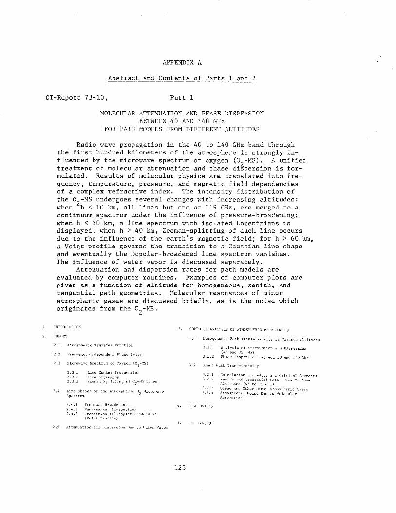
APPENDIX A
Abstract and Contents of Parts 1 and 2
OT-Report 73-10, Part 1
MOLECULAR ATTENUATION AND PHASE DISPERSION BETWEEN 40 AND 140 GHz
FOR PATH MODELS FROM DIFFERENT ALTITUDES
Radio wave propagation in the 40 to 140 GHz band through the first hundred kilometers of the atmosphere is strongly influenced by the microwave spectrum of oxygen (0
2-MS). A unified
treatment of molecular attenuation and phase dispersion is formulated. Results of molecular physics are translated into frequency, temperature, pressure, and magnetic field dependencies of a complex refractive index. The intensity distribution of the o2-Ms undergoes several changes with increasing altitudes: when h < 10 km, all lines but one at 119 GHz, are merged to a continuum spectrum under the influence of pressure-broadening; when h < 30 km, a line spectrum with isolated Lorentzians is displayed; when h > 40 km, Zeeman-splitting of each line occurs due to the influence of the earth's magnetic field; for h > 60 km, a Voigt profile governs the transition to a Gaussian line shape and eventually the Doppler-broadened line spectrum vanishes. The influence of water vapor is discussed separately.
Attenuation and dispersion rates for path models are evaluated by computer routines. Examples of computer plots are given as a function of altitude for homogeneous, zenith, and tangential path geometries. Molecular resonances of minor atmospheric gases are discussed briefly, as is the noise which originates from the o2-Ms.
1. INTRODUCTION
2. THEORY
2.1 Atmospheric Transfer Function
2, 2 Frequency-Independent Phase Delay
2.3 Microwave Spectrum of Oxygen (o2
-Ns)
2. 4
2. 3.1 Line Center Frequencies 2.3.2 Line Strengths 2. 3. 3 Zeeman Splitting of o
2-Hs Lines
Line Shapes of the Atmospheric o2
Microwave Spectrum
2. 4.1 2.4.2 2.4.3
Pressure-Broadening Nonresonant o
2-Spectrum
Transition to Doppler Broadening (Voigt Profile)
2. 5 Attenuation and Dispersion Due to Water Vapor
3. COHPUTER ANALYSIS OF ATHOSPHERIC PATH HODELS
4.
3.1 Homogeneous Path Transmissivity at Various Altitudes
3.1.1 Analysis of Attenuation and Dispersion (48 and 72 GHz)
3.1.2 Phase Dispersion Between 10 and 140 GHz
3.2 Slant Path Transmissivity
3. 2.1 Calculation Procedure and Critical Comments 3. 2. 2 Zenith and Tangential Paths From Various
Altitudes (48 to 72 GHz) 3. 2. 3 Ozone and Other Niner Atmospheric Gases 3. 2. 4 Atmospheric Noise Due to Nolecular
Absorptjon
CONCLUSIONS
5. REFERENCES
125
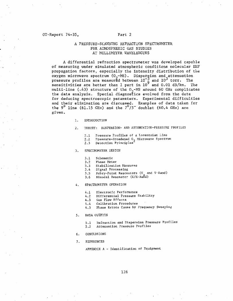
OT-Report 74-35, Part 2
A PRESSURE-SCANNING REFRACTION SPECTROMETER FOR ATMOSPHERIC GAS STUDIES
AT HILLIMETER HAVELENGTHS
A differential refraction spectrometer was developed capable of measuring under simulated atmospheric conditions molecular EHF propagation factors; especially the intensity distribution of the oxygen microwave spectrum (0
2-HS). Dispersion and attenuation
pressure profiles are measured between 10-~ and 103 torr. The sensitivities are better than 1 part in 10 and 0.01 dB/km. The multi-line (~43) structure of the o
2-HS around 60 GHz complicates
the data analysis. Special diagnosfics evolved from the data for deducing spectroscopic parameters. Experimental difficulties and their elimination are discussed. Examples of data taken for the g+ line (61.15 GHz) and the 7+;5- doublet (60.4 GHz) are given.
1, INTRODUCTION
2. THEORY: DISPERSION- AND ATTENUATION-PRESSURE PROFILES
2.1 Pressure Profiles of a Lorentzian Line 2.2 Pressure-Broadened o2 Microwave Spectrum 2.3 Detection Principles
3. SPECTROMETER DESIGN
3.1 Schematic 3.2 Phase Meter 3.3 Stabilization Measures 3.4 Signal Processing 3.5 Fabry-Perot Resonators (K and V-Band) 3.6 Bimodal Resonator (X/K-BaRd)
4. SPECTROMETER OPERATION
4.1 Electronic Performance 4.2 Differential Pressure Stability 4.3 Gas Flow Effects 4.4 Calibration Procedures 4.5 Phase Errors Cause by Frequency Sweeping
5. DATA OUTPUTS
5.1 Refraction and Dispersion Pressure Profiles 5.2 Attenuation Pressure Profiles
6. CONCLUSIONS
7 . REFERENCES
APPENDIX A - Identification of Equipment
126
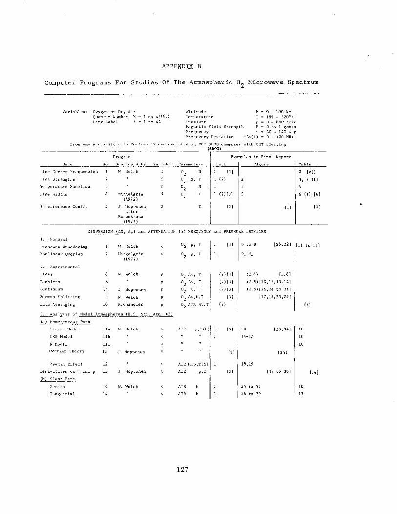
APPENDIX B
Computer Programs For Studies Of The Atmospheric o2 Microwave Spectrum
Variables: Oxygen or Dry Air Altitude h 0 - 100 km Quantum Number N = 1 to 43(63) Temperature T 180 - 320°K Line Label i = 1 to 44 Pressure p 0 - 800 torr
Magnetic Field Strength H 0 to 1 gauss Frequency \) 40 - 140 GHz Frequency Deviation ±llv(i) 0 - 100 MHz
Programs are written in Fortran IV and executed on CDC 3800 computer with CRT plotting (6600)
Program Examples in Final Report
Name No. Developed by Variable Parameters Part Figure Table
Line Center Frequencies 1 w. Welch i 02 N 1 [3] 2 [All
Line Strengths 2 i 02 N, T 1 (2) 2 3, 7 (1)
Temperature Function 3 T 02 N 1 4
Line Widths 4 Mingelgrin N 02 T 1 (2) [3] 5 6 (1) [6) (1972)
Interference Coeff. 5 J. Hopponen N T [3] [ 1] [1) after
Rosenkranz (1975)
DISPERSION (liN, li<P) and ATTENUATION (et) FREQUENCY and PRESSURE PROFILES
1. General
Pressure Broadening 6 W. Welch \) 02 p, T 1 [3] 6 to 8 [25,32) Ill to 13)
Nonlinear Overlap Mingelgrin \) 02 p, T 1 9, 21 (1972)
2. Exeerimental
Lines 8 w. Welch p 02 llv, T (2) [3] (2.4) [3,8)
Doublets 8 p 02 llv, T (2)[3] (2.5)[10,11,13.14]
Continuum 15 J. Hopponen p 02 v, T (2)[3] (2.6)[26,28 to 31)
Zeeman Splitting 9 w. Welch p 02 llv,H,T [3] [17,18,23,24)
Data Averaging 10 R.Chandler p 02 AIR llv,T (2) (7)
3. Analysis of Model AtmosEheres (U.S. Std. Atm. 62)
(a) Homogeneous Path
Linear Model lla w. Welch \) AIR p,T(h) 1 [3] 20 [33,34) 10
CMR Model llb \) 1 14-17 10
R Model llc \) 10
Overlap Theory 16 J, Hopponen \) [3) [25]
Zeeman Effect 12 \) AIR H,p,T(h) 1 18,19
Derivatives vs T and p 13 J. Hopponen \) AIR p,T [3] [35 to 38) [14) (b) Slant Path
Zenith 14 w. Welch \) AIR h 1 25 to 37 10
Tangential 14 \) AIR h 1 26 to 39 11
127
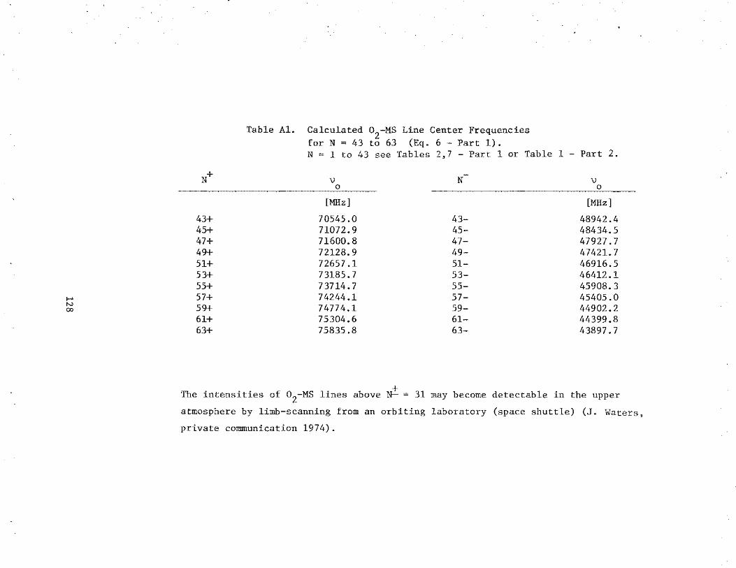
1-' N CXl
Table Al. Calculated o2
-MS Line Center Frequencies for N = 43 to 63 (Eq. 6- Part 1). N = 1 to 43 see Tables 2,7 - Part 1 or Table 1 - Part 2.
N+ \) N \) 0 0
[MHz] [MHz]
43+ 70545.0 43- 48942.4 45+ 71072.9 45- 48434.5 47+ 71600.8 47- 47927.7 49+ 72128.9 49- 47421.7 51+ 72657.1 51- 46916.5 53+ 73185.7 53- 46412.1 55+ 73714.7 55- 45908.3 57+ 74244.1 57- 45405.0 59+ 74774.1 59- 44902.2 61+ 75304.6 61- 44399.8 63+ 75835.8 63- 43897.7
The intensities of o2-MS lines above N± = 31 may become detectable in the upper
atmosphere by limb-scanning from an orbiting laboratory (space shuttle) (J. Waters,
private communication 1974).

APPENDIX C
The New Digital PRS Phase Meter
A. Diede and H. Liebe
The PRS data evaluation was improved by a completely new design
consisting of six building blocks:
1. two linear, low-noise preamplifiers for the resonance pulses
of Rl and R2;
2. two phase markers and peak detectors for dispersion and attenua-
tion measurements (Fig. Al);
3. a digital phase meter with time period averaging of dispersion
data (Fig. A2);
4. a linear ramp generator for ± klystron FM at rates,
fT = 1, 2.5, and 5 kHz;
5. a time period generator deriving the sweep rate fT and 0.1
and 0.2vs time units from a 1 MHz standard frequency; and
6. extremely well regulated power supplies (±70, ±15, ±12, ±5 V).
The circuit details are available upon request.
We mention a few of the design ideas that have been incorporated
into the new instrument. The pulses, which are detected when
sweeping the Rl(R2) resonance (Sect. 3-Part 2), are amplified in
two identical channels to a peak value of about a ~ -1 V and 0
fed into a comparator and peak detector (Fig. Al). The comparator
generates rectangular pulses whose widths correspond to the width
of the Rl(R2) resonance at a predetermined level, say 0.8 a 0
(actually variable between 0.1 a and 0.99 a). Leading and trail-a o
ing edge of each rectangular pulse are transformed into a pair of
129

•
trigger pulses identified by A1
-A2
-and B1
-B2
• It is assumed that the
resonance VRl, R2 occurs timewise in the middle between the two triggers.
The phase marking is very accurate due to high common gain and low
hysteresis of the comparator (~1 mV uncertainty).
The decrease of the R2-channel signal amplitude due to 0 -HS 2
attenuation from a + a (Eq. 39 - Part 2) is tracted by a peak detector 0 1
which, in addition, keeps the comparator level at its preset level (0.8 a1).
This AGC-scheme proved to be best in avoiding additional phase errors
introduced otherwise by o2-MS attenuation.
Dispersion (refraction) data are obtained from the time sequence
of the two pairs of triggers, A1
-A2
and within one time frame
of the FM sweep marked by S-S'. The · ~t-measurment (Eqs. 44, 49 - Part 2)
is performed by the gating logic (NAND gates Gl-G9) shown in figure A2,
which decides automatically for two cases possible in the sequence of
triggers.
Case 1. Time Duration Count Unit, ]JS
S-A 1
or S-B 1 0
Al-A2 or Bl-B2 0.2
A2-Bl or B2-Al 0.1
Bl-B2 or Al-A2 0.2
B -s' 2
or A-s' 2 0
The sequence B1-A1
-A2-B
2 when B
1-B 2 is wider than A
1-A2 produces wrong
results, but can easily be avoided by a slight offset of VRl against
130

Case 2. Time Duration Count Unit, vs
S -A 1 or S -B 1 0
Al-Bl or Bl-Al 0.2
Bl-A2 or Al-B2 0
A2-B2 or B2-A2 0.2
B -s' 2 or A-s' 2 0
The wanted time interval 6t is the total count over one sweep period.
3 4 5 The result is displayed as an average of 10 , 10 , or 10 periods.
For a sweep width u = 2.5 MHz, the sweep speed can be chosen between M
o = 2.5 (fT = 1 kHz) and 13 (fT = 5 kHz) kHz/vs while the time for a
6t-reading varies between 0.2 s (fT = 5 kHz, 103 periods) and 100 s
(fT =1kHz, 105
periods).
The performance of the new PRS phase meter is shown in figure A3 for
dispersion and attenuation detection sensitivities at three sampling rates
The most significant result is the satisfactory 6N . - detection at m1n
1 kHz with a sweep speed o = 2.55 kHz/vs. All dynamic detection problems
(phase error, p.24; amplitude error, p. 29) are reduced by a factor of 5.
The various combinations of sample number n, measurement time t0
b/6N,
and dispersion detection sensitivity X = 6N/6t give enough flexibility
to adapt to different experiment~l requirements. In addition, for
phase- and amplitude-true detection, the condition of equation (39) has
to be fulfilled.
131
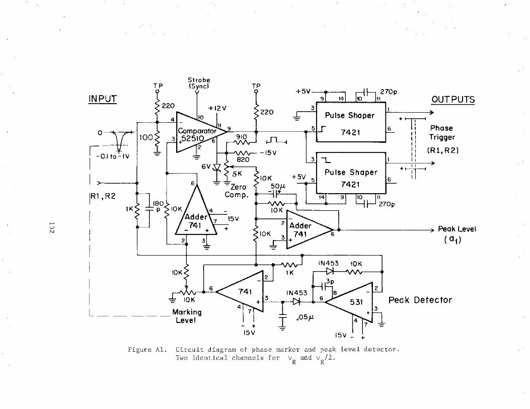
1-' (.;.)
N
Strobe TP (Sync)
y INPUT y
OT j-o.lto-IV
1001
I IR1 'R2
180 1K p ·-·"
I I L- I '"VI
I
I
I I __
-= IOK
Marking ----Level
+~
= +
TP
I +5V 270p 11 OUTPUTS
3 I ~
- Pulse Shaper +T: 5.J 7421 6 : Phase
'' T. ~ 11 ngger II
l ~ (R1, R2) 3 .,_ 1 l1
) II
Pulse Shaper +T +5V 5 6 7421
s I() I( I '""uut:r 7.dt ~· Peak Level
( 01) I ~ ~
Peak Detector
.05fL
Figure Al. Circuit diagram of phase marker and peak level detector. Two identical channels for VR and VR/2.
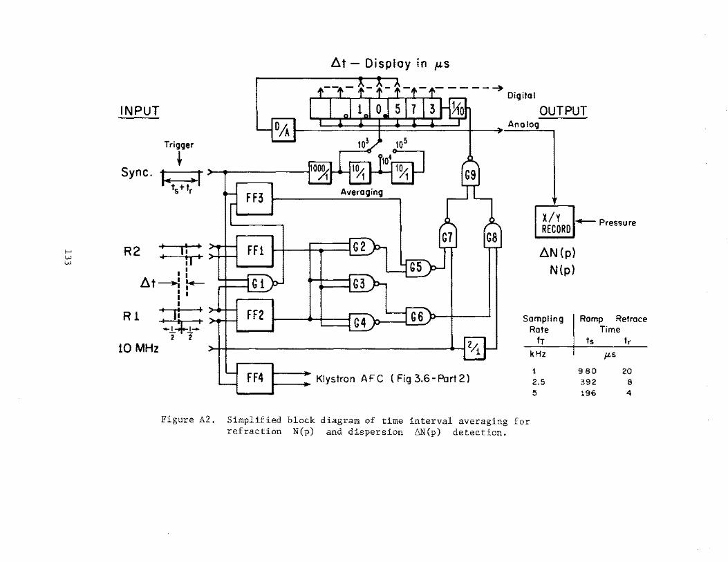
,_.. w w
INPUT
Trigger
~ Sync. 1 1
Ill( )1>-
ts+tr
R2 ' li · I :1 I
I I I
~t-.: ~ I I I I
R 1 I u I I+ I -.l .l-2 2
10 MHz
FF3
FF1
~t- Display in p.s
-----~Digital
OUTPUT , , I Analog I I.' I'' )I
Klystron AFC (Fig 3.6-Part2)
X/Y 1.._ Pressure RECORD
~N(p)
N(p)
Sampling Rote
fr kHz
1
2.5 5
Romp Retrace Time
ts tr JLS
980 20 392 8 196 4
Figure A2. Simplified block diagram of time interval averaging for refraction N(p) and dispersion 6N(p) detection.
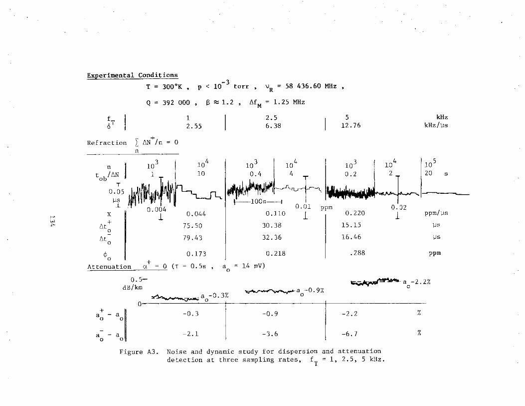
1-' w +:'-
Experimental Conditions
T = 300°K -3 p < 10 torr , vR = 58 436.60 MHz
Q = 392 000 B ~ 1.2
fT 0
. \ + Refract1on L ~N /n = 0 n
n 103
1 t /~N
ob o~~s~~ .1. .~n o.oo4
X I 1 +
~to
~to
1 2.55
104
10
0.044
75.50
79.43
¢ 1 o.l73 0 +
Attenuation a = 0 (T = 0.5s a 0
~fM = 1. 25 MHz
2.5 6.38
0.110
30.38
32.36
0.218
14 mV)
104
4
0.01
1 ppm
5 12.76
103
0.2
0.220
15.15
16.46
.288
104
2
0.02 l
kHz kHz/]Js
105
20 s
ppm/]Js
]JS
]JS
ppm
0.5-dB/km
o-···~ao-0.3% ~ao-0.9% ~-a0-2.2%
+ a - a 0 0
a - a 0 0
-0.3
-2.1
I
I ~::: I -2.2
-6.7
Figure A3. Noise and dynamic study for dispersion and attenuation detection at three sampling rates, fT = 1, 2.5, 5 kHz.
%
%
APPENDIX D
Activities Under Joint Sponsorship (see Preface)
Research Period: 14 January 1971 to 28 February 1975
Personnel: The following made scientific and technical contributions to the work reported in the Final Report (Parts 1 to 3):
Principal Investigator: H. J. Liebe
Research Associates w. M. Welch u. Mingelgrin T. A. Dillon G. G. Gimmestad
Research Engineers M. J. Vetter R. Chandler A. Diede R. May
Programmer J. Hopponen
Reporting: 38 monthly progress letters have been written
*) Presentations at Meetings:
Liebe and Welch, "Atmospheric transmissivity between 48 and 72 GHz for vertical and horizontal path models at various altitudes," Symp. Antennas and Propagation, IEEE G-AP, Denver, CO, June, 1971.
Mingelgrin, "The effect of pressure and temperature on the o2 microwave spectrum ..• ," CIRES Seminar, Boulder, CO, November, 1971.
Liebe and Welch, "Complex atmospheric transmission factor between 48 and 72 GHz of various altitudes," URSI Fall Meeting, Los Angeles, September, 1971, (p. 14).
Mingelgrin and tion phenomena Physics Conf.,
Gordon, of 0 " 2' London,
"Study of some spectra and relaxa-4th National Atomic and Molecular April, 1972, (p. 12).
Welch, Mingelgrin, and Liebe, "Quantitative studies of the pressure-broadened microwave spectrum of o2 ," First Internat. Conf. on Spectral Lines, APS, Knoxville, TN, August, 1972.
135

Liebe and Welch, "Pressure-scanning microwave spectroscopy for quantitative studies of resonant and nonresonant spectra," Second European Microwave Spectroscopy Conf., Bangor, Wales, September, 1972.
Liebe, Recommendations to NSF Workshop on "Future directions of electromagnetics of continuous media," Williamsburg, VA, December, 1972.
j "Laboratory measurements and analysis of propagation factors between 20 and 100 GHz," IEEE/AP-S Symposium, NCAR, Boulder, CO, May, 1974.
, "Laboratory studies of the atmospheric microwave spectrum of oxygen and water vapor," 5th Colloquium on Microwave Communication, Budapest, June, 1974.
, "Oxygen microwave attenuation from laboratory measurements," Third Annual Conf. Telecommunications for Government, Boulder, CO, October, 1974.
, "A pressure scanning EHF spectrometer for atmospheric gas studies," 1974 USNC/URSI-IEEE Meeting Boulder, CO, October, 1974.
"Role of spectroscopy in microwave propagation," EMWave Seminar (OT-NOAA-CIRES-CU Series), Boulder, CO, February, 1975.
, "Absolute intensity measurements of the 60 GHz oxygen band under simulated atmospheric conditions," Inter-Union Commission on Radio Meteorology, URSI-IUGG Workshop, Bournemouth, England, May, 1975.
Also, see under Publications No. 1, 2, 6, 9, 11, and 15.
Publications*)
1. Liebe and Welch, "Phase delay and attenuation in the 50 to 70 GHz band for atmospheric path models at various altitudes," Proc. Internat. Symp. Ant. & Propagation, Sendai, Japan, September, 1971, 239-240 (published by IECE of Japan).
2. Liebe, "Precise measurements of atmospheric propagation parameters in the 50 to 75 GHz band using pressure scanning spectroscopy," Proc. NASA-AAFE Conference. October, 1971, 276-292 (published by NASA/LRC).
*) which carry an acknowledgement of NOAA, NASA, and/or DoD-ARO support (see Preface)
136
3. Dillon and Liebe, "Dispersion studies of the 22 GHz water vapor line shape. Part II," J. Quant. Spectr. Rad. Trans f. 11, 1803-1817' 1971.
4. Welch and Mizushima, "Molecular parameters of the o2 molecule," Phys. Rev. A-5, 2692-2696 (1972).
5. Welch, Liebe, and Dougherty, "W-Band study (50-75 GHz)," Final Report on ITS Project 910 1383, February 1972, 15 pp.
6. Liebe, Atmospheric transmissivity in the 48 to 72 GHz band. Analysis and Laboratory Measurements, "IEEE Internat. Conf. on Communications, Philadelphia, June, 1972; IEEE Cat. No. 72 CHD-622-1 Com, 41/16-22.
7. Mingelgrin, "Classical scattering calculations for diatomic molecules and application to microwave spectrum of o2 ," TRE-32, July, 1972 (U.S. Govt. Printing Office, Washington, D.C.), 58 pp.
8. Liebe, "Complex atmospheric transmission response between 35 and 140 GHz -Programs I and II," OT-ITS Catalog of Telecommunication Related Computer Programs, November, 1971, 216-219.
9. Liebe and Welch, "Laboratory measurements and analysis of atmospheric propagation parameters in the 30 to 72 GHz band," NATO-AGARD Conference Print No. 107, 5/1-20 (18th Meeting of E.M. Wave Prop. Panel), Gausdal, Norway, September, 1972.
10. Mizushima, Wells, Evenson, and Welch, "Laser magnetic resonance of the o2 molecule," Phys. Rev. L. ~. 831-833, 1972.
11. Liebe, Welch, and Chandler, "Labor a tory measurmen t s of e. m. properties of atmospheric gases at millimeter wavelengths, IEE Conference Publ. No. 98, 244-249 (Conf. on Propagation of Radio Waves Above 10 GHz) London, April, 1973.
12. Liebe and Welch, "Molecular attenuation and phase dispersion between 40 and 140 GHz for path models from different -Part 1-altitudes," OT-Report 73-10, May, 1973, 104 pp. (U.S. Govt. Printing Office, Washington, D.C.).
13. Liebe, "A pressure-scanning refraction spectrometer for atmospheric gas studies at millimeter wavelengths," -Part 2-0T-Report 74-35, April, 1974, 132 pp. (U.S. Govt. Print-ing Office, Washington, D.C.).
14. Mingelgrin, "The microwave dispersion spectrum of o2 ," Molecular Physics, 28, 1591-1602, (1974).
137
15. Liebe and Welch, "Laboratory measurements and analysis of atmospheric propagation factors between 20 and 100 GHz," 1974 MmWaves Techniques Conference, NELC - San Diego, March, 1974, B2/l-6.
16. Liebe, "Molecular EHF transfer characteristics of air," Chapter C.VIII in Handbook "Multipath in the Air Traffic Control Frequencies," (W. J. Hartman, editor), Report No. FAA-74-75, vol. II, pp. 1-33, July, 1974 (available from NTIS, Springfield, Virginia 22151).
17. Liebe, "Transfer characteristics of clear air between 10 and 150 GHz," contribution to NASA Active Microwave Workshop Handbook, Sect. 4.4.4, pp. 205-236, July, 1974.
18. Liebe, "Molecular transfer characteristics of air between 40 and 140 GHz," IEEE Trans. MTT-23, 380-386, 1975.
19. Liebe, "Studies of oxygen and water vapor microwave spectra under simulated atmospheric conditions," OT Report 75-65, June, 1975, 150 pp. (this report).
20. Liebe, "A pressure-scanning millimeter-wave dispersion spectrometer," Rev. Sci. Instr. 46, July, 1975.
21. Liebe and Hopponen, "Temperature and pressure sensitivities of air transfer characteristics between 40 and 140 GHz," in preparation for Radio Science.
138
-Part 3-

FORM OT-29 U.S. DEPARTMENT OF COMMERCE (3•73) OFFICE OF TELECOMMUNICATIONS
BIBLIOGRAPHIC DATA SHEET
1. PUBLICATION OR REPORT NO 2. Gov't Accession No. 3. Recipient's Accession No.
OTR 75-65
4. TITLE AND SUBTITLE 5. Publication Date
Studies of oxygen and water vapor microwave spectra June 1975 under simulated atmospheric conditions. 6. Performing Organization Code
OT/ITS, Div. 3 7. AUTHOR(S) 9, Project/Task/Work Unit No.
!Hans J. Liebe 910 1411 (a) 8. PERFORMING ORGANIZATION NAME AND ADDRESS 910 1410 (b)
u.s. Department of Connnerce 910 5204 (OT) OT/ITS I 0. Contract/Grant No.
325 Broadway (a) NASA-AAFE L58, 506 Boulder, co 80302 (b) NOAA-NESS 5-13155 II. Sponsoring Organization Name and Address 12. Type of Report and Period Covered
(a) NASA Langley Research Center, Hampton, VA 23365 OT Report * (b) NOAA-National Environmental Satellite Service, (Final Report, Part III) Suitland, MD 20233 13.
14. SUPPLEMENTARY NOTES
~~Part I is OT Report 73-10, Part II is OT Report 74-35
15. ABSTRACT (A 200·word or less factual sununary of most significant information. If document includes a significant bibliography ot literature survey, mentioo it here.)
Atmospheric radio wave propagation in the 40 to 140 GHz band is influenced by microwave spectra of oxygen (0 -MS) and water vapor. The report treats the complementary roles of controlled laboratory experiments and computer analysis for providing detailed molecular transfer characteristics. A pressure-scanning differential refractometer was operated at fixed frequencies between 58 and 61.5 GHz. ,The variability of 0~ and H2o spectra with frequency, pressure, tempera-ture, and magnetic field streng h was studied under conditions which occur in the atmosphere. Results obtained (a) for oxygen and air on the 9+ line, the 7+/5- and 3+/9- doublets, and the continuum spectrum, and (b) for water vapor on nonresonant effects, are reported. The experimental o2-Ms data are used in theoretical analyse of attenuation and dispersion rates which are extended to other lines, to fre-quencies identified for remote sensing applications, and to temperature and pressure sensitivities between 40 and 140 GHz.
16. Key words (Alphabetical order, separated by semicolons)
Atmospheric mm-wave propagation; attenuation profiles; dispersion profiles; EHF transfer characteristics; oxygen microwave spectrum; water vapor microwave spectrum.
17. AVAILABILITY STATEMENT
[KJ UNLIMITED.
D FOR OFFICIAL DISTRIBUTION.
1:J. U.S. GOVERNMENT PRINTING OFFICE 1975- 680·794/232 Reg. 8
18. Security Class (Ihis report)
Unclassified
19, Security Class (Ihis page)
Unclassified
20. Number of pages
150
21. Price:
LISCOMM·OC 297111·P73 USCOMM ·Ell