STUDIES IN GRAPH THEORY - DISTANCE RELATED CONCEPTS IN...

STUDIES IN GRAPH THEORY - DISTANCE RELATED

CONCEPTS IN GRAPHS

A THESIS

Submitted by

R. ANANTHA KUMAR (Reg. No. 200813107)

In partial fulfillment for the award of the degree

of

DOCTOR OF PHILOSOPHY

FACULTY OF SCIENCE AND HUMANITIES

KALASALINGAM UNIVERSITY

(KALASALINGAM ACADEMY OF RESEARCH AND EDUCATION)

ANAND NAGAR, KRISHNANKOIL – 626 126

TAMIL NADU, INDIA.

SEPTEMBER 2013

CERTIFICATE

This is to certify that all the corrections/suggestions pointed out by the examiners

have been incorporated in the thesis of Mr. R. ANANTHA KUMAR.

Place: Krishnankoil SIGNATURE Date: 21-06-2014 Dr. S. ARUMUGAM SUPERVISOR

Senior Professor (Research) National Centre for Advanced Research in Discrete Mathematics (n-CARDMATH)

Kalasalingam University (Kalasalingam Academy of Research and Education)

Anand Nagar, Krishnankoil – 626 126, Tamil Nadu, INDIA.

KALASALINGAM UNIVERSITY (Kalasalingam Academy of Research and Education)

ANAND NAGAR, KRISHNANKOIL 626 126

BONAFIDE CERTIFICATE

Certified that this thesis titled “STUDIES IN GRAPH THEORY - DISTANCE

RELATED CONCEPTS IN GRAPHS” is the bonafide work of

Mr. R. ANANTHA KUMAR, who carried out the research under my

supervision. Certified further that to the best of my knowledge the work reported

herein does not form part of any other thesis or dissertation on the basis of which

a degree or award was conferred on an earlier occasion of this or any other

candidate.

SIGNATURE Dr. S. ARUMUGAM SUPERVISOR

Senior Professor (Research) National Centre for Advanced Research in Discrete Mathematics (n-CARDMATH)

Kalasalingam University (Kalasalingam Academy of Research and Education)

Anand Nagar, Krishnankoil – 626 126, Tamil Nadu, INDIA.

ABSTRACT

By a graph G = (V,E), we mean a finite undirected graph

with neither loops nor multiple edges. The order and size of G are

denoted by n = |V | and m = |E| respectively. For graph theoretic

terminology we refer to Chartrand and Lesniak [7].

In Chapter 1, we collect some basic definitions and

theorems on graphs which are needed for the subsequent chapters.

The distance d(u, v) between two vertices u and v of a con-

nected graph G is the length of a shortest u-v path in G. There are

several distance related concepts and parameters such as

eccentricity, radius, diameter, convexity and metric dimension which

have been investigated by several authors in terms of theory and

applications. An excellent treatment of various distances and

distance related parameters are given in Buckley and Harary [6].

Let G = (V,E) be a graph. Let v ∈ V . The open neigh-

borhood N(v) of a vertex v is the set of vertices adjacent to v. Thus

N(v) = w ∈ V : wv ∈ E. The closed neighborhood of a vertex v,

is the set N [v] = N(v) ∪ v. For a set S ⊆ V, the open neighbor-

hood N(S) is defined to be⋃v∈S

N(v). For any two disjoint subsets

A, B ⊆ V, let [A,B] denote the set of all edges with one end in A

and the other end in B. For any set C ⊆ V, the induced subgraph

〈C〉 is the maximal subgraph of G with vertex set C.

Saenpholphat and Zhang [25] introduced the concept of

connected resolving set and in this context they introduced the con-

cept of distance similar vertices. Two vertices u and v of a connected

graph G are defined to be distance similar if d(u, x) = d(v, x) for

all x ∈ V (G) − u, v. Hence two vertices u and v in a connected

graph G are distance similar if and only if either uv /∈ E(G) and

N(u) = N(v) or uv ∈ E(G) and N [u] = N [v]. Also, distance sim-

ilarity in a connected graph G is an equivalence relation on V (G).

Therefore this relation gives a unique partition of V (G). We ob-

serve that if U is a distance similar equivalence class of G, then

|d(x, v) : v ∈ U| = 1 for all x ∈ V − U. These observations lead

to the following concepts.

Let G = (V,E) be a connected graph. A proper subset S

of V is called a distance similar set if |d(u, v) : v ∈ S| = 1 for all

u ∈ V − S. A distance similar set S is called a maximal distance

similar set if any set S1 with S ( S1 ( V, is not a distance similar

set of G. The maximum cardinality of a maximal distance similar

set of G is called the distance similar number of G and is denoted by

ds(G). The minimum cardinality of a maximal distance similar set

in G is called the lower distance similar number of G and is denoted

by ds−(G). Any distance similar set S of G with |S| = ds(G) is

called a ds-set of G.

A nonempty subset S of V is called a pairwise distance

similar set (pds-set) if either |S| = 1 or any two vertices in S

are distance similar. The maximum cardinality of a maximal pair-

iv

wise distance similar set in G is called the pairwise distance similar

number of G and is denoted by Φ(G). The minimum cardinality

of a maximal pairwise distance similar set in G is called the lower

pairwise distance similar number of G and is denoted by Φ−(G).

Let V1, V2, . . . , Vk be the distance similar equivalence classes

of G. Then Φ(G) = max1≤i≤k

|Vi| and Φ−(G) = min1≤i≤k

|Vi|.

In Chapter 2, we obtain a condition for S ⊆ V to be a

distance similar set of a graph G and a condition for a maximal

distance similar set to be a distance similar equivalence class of G.

We characterize bipartite graphs and unicyclic graphs with ds(G) =

1. We give a relation connecting dim(G) and cardinality of maximal

distance similar sets. We characterize graphs with distance similar

number equal to ∆(G), n− 2, n− 3 and d(G). We also determine

the distance similar number for several product graphs.

We show that the set of all maximal distance similar sets

which are contained in any neighborhood N(u) forms a partition of

N(u). We also prove that the distance similar number of any graph

can be computed in polynomial time.

In Chapter 3, we initiate a study of pairwise distance sim-

ilar set and pairwise distance similar number of a graph. Let Φ(G)

and Φ−(G) denote the pairwise distance similar number and lower

pairwise distance similar number of a graph G. We present several

basic results on these parameters. We obtain a characterization of

graph with Φ(G) = ∆(G) and Φ−(G) = ∆(G). We present sharp

v

lower and upper bounds of Φ(G) for product graphs. Further we

characterize graphs with Φ(G) = n− 2 and Φ(G) = n− 3.

One of the basic problems in graph theory is to select a

minimum set S of vertices in such a way that each vertex in the

graph is uniquely determined by its distances to the chosen ver-

tices. This concept was introduced by Slater [29] who called such

a set as a locating set. The same concept was independently dis-

covered by Harary and Melter [16] who used the term resolving set.

By an ordered set of vertices we mean a set W = w1, w2, · · · , wk

on which the ordering (w1, w2, · · · , wk) has been imposed. For an

ordered subset W = w1, w2, · · · , wk of V (G), we refer to the

k-vector (ordered k-tuple) r(v|W ) = (d(v, w1), d(v, w2), · · · , d(v, wk))

as the (metric) representation of v with respect to W . The set W

is called a resolving set for G if r(u|W ) = r(v|W ) implies u = v for

all u, v ∈ V (G). Hence if W is a resolving set of cardinality k for

a graph G of order n, then the set r(v|W ) : v ∈ V (G) consists

of n distinct k-vectors. A resolving set of minimum cardinality is

called a basis for G. The metric dimension of G is defined to be the

cardinality of a basis of G and is denoted by dim(G).

The definition of metric dimension of a graph depends on

the concept of resolving set W, in which an order is imposed on the

elements of W. We define the concept distance pattern distinguish-

ing sets in which W is considered simply as a set and for any vertex

v the set of all distances from v to W is associated.

vi

Let M be a nonempty subset of V (G) and let u ∈ V (G).

The distance pattern of u with respect to M is given by fM(u) =

d(u, v) : v ∈M. If fM is an injective function on V, then the set M

is called a distance pattern distinguishing set (DPD-set) of G. If G

admits a DPD-set, then G is called a DPD-graph. The minimum

cardinality of a DPD-set in a DPD-graph G is the DPD-number

of G and is denoted by %(G).

In Chapter 4, we study distance pattern distinguishing sets

and distance pattern distinguishing number of a graph. We obtain

several necessary conditions for distance pattern distinguishing sets,

and characterize some families of graphs which admit a distance pat-

tern distinguishing set. We also obtain distance pattern distinguish-

ing number of several families of graphs. Further, we give a relation

connecting distance pattern distinguishing number and metric di-

mension of a graph. We define the concept local distance pattern

distinguishing set (LDPD-set) and LDPD-number of a graph G.

We obtain LDPD-number of several families of graphs.

Maximum matchings in bipartite graphs have several

interesting applications. Let G = (V, E) be a bipartite graph with

bipartition V1 and V2, where |V1| ≤ |V2|. Hall [15] proved that there

exists a matching M in G such that V1 is matched to a subset of V2

under M if and only if |N(S)| ≥ |S| for all S ⊆ V1.

The condition |N(S)| ≥ |S| for all S ⊆ V is called Hall’s

condition. Motivated by this condition Chartrand and Lesniak [7]

defined a subset U of V to be nondeficient if |N(S)| ≥ |S| for every

vii

nonempty subset S of U. We introduce the concept of nondeficient

number ofG. The nondeficient number nd(G) of a graphG is defined

to be the maximum cardinality of a nondeficient set of G. Any

nondeficient set U of G with |U | = nd(G) is called a nd-set of G.

In Chapter 5, we initiate a study of nondeficient number

of graphs. We also present sharp lower and upper bounds for non-

deficient number. We obtain several bounds for nd(G) in terms of

well known graph theoretic parameters such as β0 and β1. Further

we give a relation connecting nondeficient number and order of a

maximum critical independent set.

viii

ACKNOWLEDGEMENT

First of all, I thank Almighty God for His abundant blessings.

I am indebted and grateful to my supervisor Prof. S. Arumugam,

Director, n-CARDMATH, Kalasalingam University, Krishnankoil for his invalu-

able guidance, inspiration and fruitful discussions during the course of this

research work.

My special thanks are due to our collaborators Prof. S. B. Rao,

Dr. B .D. Acharya and Dr. K.A. Germina.

I wish to express my thanks to the Department Research Committee

Members for their helpful suggestions.

I thank the Department of Science and Technology (DST),

Government of India, New Delhi for providing financial assistance through

Research Fellowship during the period August 2008 - August 2011 at Kalasalingam

University.

I am extremely thankful to the Chairman, A.K. Group of Institu-

tions “Kalvivallal” Thiru T. Kalasalingam, Chancellor “Ilayavallal” Thiru

K. Sridharan and Vice-Chancellor Dr. S. Saravanasankar, Kalasalingam

University for providing the necessary facilities during the period of my research.

I also thank the staff members and research scholars of n-CARDMATH for their

kind cooperation.

Words are inadequate to express my gratitude to my parents and other

members of my family for their affectionate blessings and support throughout my

academic career. I heartily thank my friends for their constant encouragement to

finish this work successfully.

It is my pleasure to thank Prof. S. Arumugam’s family for their

affection.

Finally, I extend my thanks to Mr. K. Alaguraj, for typesetting the

thesis in an excellent manner.

R.ANANTHA KUMAR

ix

TABLE OF CONTENTS

TITLE PAGE NO.

ABSTRACT iii

LIST OF FIGURES xii

LIST OF SYMBOLS xiii

CHAPTER 1. PRELIMINARIES 1

1.1 INTRODUCTION 1

1.2 BASIC GRAPH THEORY 1

1.3 DISTANCE RELATED CONCEPTS 9

1.4 ORGANIZATION OF THE THESIS 13

CHAPTER 2. DISTANCE SIMILAR SETS 15

IN GRAPHS

2.1 INTRODUCTION 15

2.2 BASIC RESULTS 16

2.3 AN ALGORITHM FOR COMPUTING ds(G) 21

2.4 GRAPHS WITH ds(G) = 1 25

2.5 DISTANCE SIMILAR SETS AND

RESOLVING SETS 27

2.6 BOUNDS FOR DISTANCE SIMILAR NUMBER 28

2.7 DISTANCE SIMILAR SETS AND

GRAPH OPERATIONS 33

2.8 CONCLUSION AND SCOPE 38

x

TITLE PAGE NO.

CHAPTER 3. PAIRWISE DISTANCE SIMILAR 39

SETS IN GRAPHS

3.1 INTRODUCTION 39



CHAPTER 4. DISTANCE PATTERN 49

DISTINGUISHING SETS IN GRAPHS

4.1 INTRODUCTION 49


4.3 DPD-NUMBER OF GRAPHS 56

4.4 METRIC DIMENSION AND DPD-NUMBER 64

4.5 EMBEDDING A GRAPH INTO A DPD-GRAPH 70

4.6 LOCAL DPD-SETS 72

4.7 LDPD-GRAPHS AND UNIVERSAL VERTICES 82


CHAPTER 5. NONDEFICIENT SETS IN GRAPHS 92

5.1 INTRODUCTION 92


5.3 BOUNDS 101

5.4 NONDEFICIENT SETS AND GRAPH

OPERATIONS 106


REFERENCES 113

LIST OF PUBLICATIONS 117

VITAE 118

xi

LIST OF FIGURES

FIGURE TITLE PAGE

NO. NO.

2.1 Graph with ds = 4 and ds− = 1 17

2.2 Example for distance similarity is not hereditary 21

2.3 Example for illustration of Algorithm 2.3.1 24

3.1 Graph with Φ = 4 and Φ− = 1 41

3.2 Graphs with unequal and equal Φ and Φ− 42

3.3 Graph with ds = 4 and Φ = 1 43

3.4 Graph with Φ = n− 3 46

4.1 DPD-Graph 51

4.2 Graph which is LDPD but not DPD 74

5.1 Tree with n− (|Ic| − |N(Ic)|) = 4 and nd(T ) = 4 106

5.2 Graph G2 109

xii

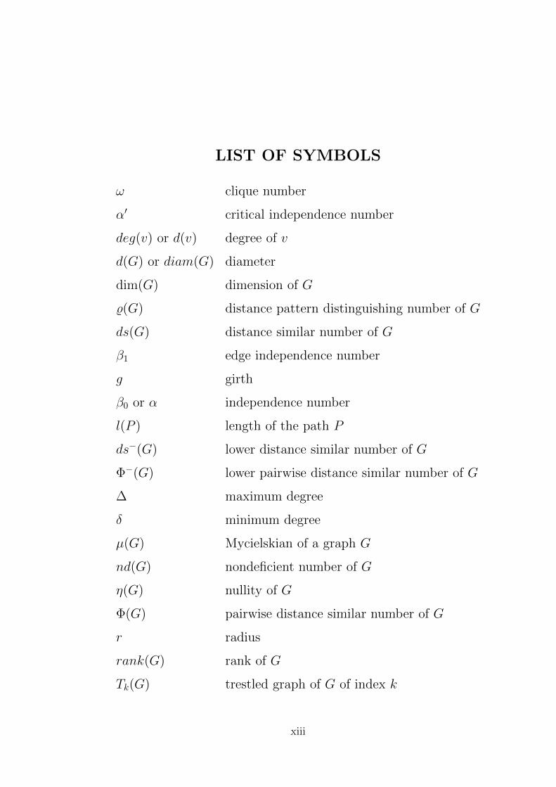
LIST OF SYMBOLS

ω clique number

α′ critical independence number

deg(v) or d(v) degree of v

d(G) or diam(G) diameter

dim(G) dimension of G

%(G) distance pattern distinguishing number of G

ds(G) distance similar number of G

β1 edge independence number

g girth

β0 or α independence number

l(P ) length of the path P

ds−(G) lower distance similar number of G

Φ−(G) lower pairwise distance similar number of G

∆ maximum degree

δ minimum degree

µ(G) Mycielskian of a graph G

nd(G) nondeficient number of G

η(G) nullity of G

Φ(G) pairwise distance similar number of G

r radius

rank(G) rank of G

Tk(G) trestled graph of G of index k

xiii

CHAPTER 1

PRELIMINARIES

1.1 INTRODUCTION

In this chapter we collect some basic definitions and

theorems on graphs which are needed for the subsequent chapters.

For graph theoretic terminology, we refer to Chartrand and Lesniak

[7].

In Section 1.2 we present some of the basic definitions in

graph theory. In Section 1.3 we present the fundamentals of distance

similar vertices and nondeficient sets in graphs. In Section 1.4 we

give an overview of the organization of the remaining chapters of

the thesis.

1.2 BASIC GRAPH THEORY

Definition 1.2.1. A graph G is a finite nonempty set of objects

called vertices together with a set of unordered pairs of distinct

vertices of G called edges. The vertex set and the edge set of G are

denoted by V (G) and E(G) respectively. The edge e = u, v is

said to join the vertices u and v . We write e = uv and say that

u and v are adjacent vertices; u and e are incident, as are v and e.

If e1 and e2 are distinct edges of G incident with a common vertex,

then e1 and e2 are adjacent edges.

The number of vertices in G is called the order of G and

the number of edges in G is called the size of G. The order and size

of G are denoted by n and m respectively. A graph is trivial if its

vertex set is a singleton.

Definition 1.2.2. Let G = (V,E) be a graph and let v ∈ V. A

vertex u is called a neighbor of v in G if uv is an edge of G. The

set N(v) of all neighbors of v is called the open neighborhood of v.

Thus N(v) = u ∈ V : uv ∈ E. The closed neighborhood of v in G

is defined as N [v] = N(v) ∪ v. If S ⊆ V, then N(S) =⋃v∈S

N(v)

and N [S] = N(S) ∪ S.

Definition 1.2.3. The degree of a vertex v in a graph G is de-

fined to be the number of edges incident with v and is denoted

by deg(v) or d(v). In other words deg(v) = |N(v)|. The minimum

and maximum degrees of vertices of G are denoted by δ and ∆

respectively.

A vertex of degree zero in G is called an isolated vertex

and a vertex of degree one is called a pendant vertex or a leaf. An

edge e in a graph G is called a pendant edge if it is incident with a

pendant vertex. Any vertex which is adjacent to a pendant vertex

is called a support vertex. A vertex of degree n − 1 is called an

universal vertex.

2

Definition 1.2.4. A walk W in a graph G is an alternating se-

quence u0, e1, u1, . . . , uk−1, ek, uk of vertices and edges of G, begin-

ning and ending with vertices, such that ei = ui−1ui, for 1 ≤ i ≤ k.

The vertices u0 and uk are called the origin and terminus of W re-

spectively and W is called a u0-uk walk. The walk W is also denoted

by (u0, u1, u2, . . . , uk−1, uk). If u0 = uk, the walk is closed and open

otherwise. The number of edges in a walk is called the length of the

walk. A path P of length k (denoted by Pk) is a walk (u0, u1, u2,

. . . , uk−1, uk) in which all the vertices u0, u1, u2, . . . , uk−1, uk are

distinct.

Definition 1.2.5. A cycle Ck of length k ≥ 3 in a graph G

is a closed walk (u0, u1, u2, . . . , uk−1, u0) in which all the vertices

u0, u1, u2, . . . , uk−1 are distinct. A cycle Ck is called even or odd

according as k is even or odd.

A graph G having no cycle is called an acyclic graph. A

graph having exactly one cycle is called an unicyclic graph. The

length of a shortest cycle (if any) in a graph G is called its girth and

denoted by g(G).

Definition 1.2.6. A graph G is said to be connected if every pair

of distinct vertices of G are joined by a path. A graph G that is

not connected is called a disconnected graph. A maximal connected

subgraph of G is called a component of G. Thus a disconnected

graph is a graph having more than one component.

3

Definition 1.2.7. A graph G is complete if every pair of distinct

vertices of G are adjacent in G. A complete graph on n vertices is

denoted by Kn.

A clique in G is a complete subgraph of G. The maximum

order of a clique in G is called the clique number of G and is denoted

by ω(G) or simply ω. A clique H in G with |V (H)| = ω is called a

maximum clique in G.

Definition 1.2.8. The complement G of a graph G is the graph

with vertex set V (G) such that two vertices are adjacent in G if and

only if they are not adjacent in G.

Definition 1.2.9. A nontrivial connected graph having no cut

vertex is called a block. A block of a graph G is a subgraph of G

which itself is a block and is maximal with respect to this property.

For any real number x, bxc denotes the largest integer

less than or equal to x and dxe denotes the smallest integer greater

than or equal to x.

Definition 1.2.10. A graph H is called a subgraph of G if

V (H) ⊆ V (G) and E(H) ⊆ E(G). A subgraph H of a graph G is

a proper subgraph of G if either V (H) 6= V (G) or E(H) 6= E(G). A

spanning subgraph of G is a subgraph H of G with V (H) = V (G).

4

For a set S of vertices of G, the induced subgraph denoted

by 〈S〉 or by G[S], is the maximal subgraph of G with vertex set S.

Thus two vertices of S are adjacent in 〈S〉 if and only if they are

adjacent in G.

For any two disjoint subsets A, B ⊆ V, let [A,B] denote

the set of all edges with one end in A and the other end in B.

Definition 1.2.11. Two graphs G1 and G2 are said to be isomor-

phic (written as G1∼= G2) if there exists a bijection φ : V (G1) →

V (G2) such that uv ∈ E(G1) if and only if φ(u)φ(v) ∈ E(G2). Such

a function φ is called an isomorphism from G1 to G2.

Definition 1.2.12. A bipartite graph G = (X, Y,E) is a graph

whose vertex set V (G) can be partitioned into two nonempty subsets

X and Y such that each edge of G has one end in X and the other

end in Y. The pair (X, Y ) is called a bipartition of G.

Definition 1.2.13. A complete bipartite graph Kr,s is a bipartite

graph G with bipartition X, Y such that |X| = r, |Y | = s and every

vertex in X is adjacent to every vertex in Y. The graph K1,r is called

a star. When r > 2, the vertex of degree r in K1,r is called its center.

The graph G obtained from K1,r and K1,s by joining their centers

by an edge is called a bistar and is denoted by B(r, s).

5

Definition 1.2.14. A k-partite graph G is a graph whose vertex

set V can be partitioned into k nonempty subsets V1, V2, . . . , Vk such

that no edge has both ends in any one subset Vi. If furtherG contains

every edge uv where u ∈ Vi, v ∈ Vj, i 6= j, then G is called a complete

k-partite graph and is denoted by Kn1,n2,...,nkwhere |V1| = n1, |V2| =

n2, . . . , |Vk| = nk.

Definition 1.2.15. A subset S ⊆ V is said to be independent if

no two vertices in S are adjacent. The independence number β0(G)

is the maximum cardinality of an independent set in G.

Definition 1.2.16. A connected acyclic graph is called a tree. A

disconnected graph in which each component is a tree is called a

forest.

Definition 1.2.17. Two graphs G1 and G2 are said to be disjoint

if they have no vertex in common. They are said to be edge disjoint

if they have no edge in common.

Definition 1.2.18. Let G1 and G2 be two graphs with disjoint

vertex sets.

1. The union G = G1 ∪ G2 has V (G) = V (G1) ∪ V (G2) and

E(G) = E(G1) ∪ E(G2). A graph G consisting of k, k ≥ 2

disjoint copies of a graph H is denoted by G = kH.

6

2. The join G = G1 +G2 has V (G) = V (G1)∪V (G2) and E(G) =

E(G1) ∪ E(G2) ∪ uv : u ∈ V (G1), v ∈ V (G2).

3. The Cartesian productG = G1G2 has V (G) = V (G1)× V (G2),

and two vertices (u1, u2) and (v1, v2) of G are adjacent in G if

and only if either u1 = v1 and u2v2 ∈ E(G2) or u2 = v2 and

u1v1 ∈ E(G1).

4. The corona of G1 and G2 is defined to be the graph G = G1G2

formed from one copy of G1 and |V (G1)| copies of G2 where the

ith vertex of G1 is adjacent to every vertex in the ith copy of G2.

In particular, the corona H K1 is the graph constructed from

a copy of H, where for each vertex v ∈ V (H), a new vertex v′

and a pendant edge vv′ are added.

5. The Lexicographic product G ∗ H of two graphs G and H has

V (G∗H) = V (G)×V (H) and two vertices (u, x), (v, y) of G∗H

being adjacent whenever uv ∈ E(G), or u = v and xy ∈ E(H).

6. For three or more disjoint graphs G1, G2, . . . , Gn the sequential

join G1 +G2 + · · ·+Gn is the graph (G1 +G2) ∪ (G2 +G3) ∪

· · · ∪ (Gn−1 +Gn).

Definition 1.2.19. A split graph is a graph whose vertex set can

be partitioned into two sets V1 and V2 such that V1 forms a complete

graph and V2 is an independent set.

Definition 1.2.20. The hypercube Qn is the graph whose ver-

tices are the n-dimensional binary vectors, where two vertices are

7

adjacent if and only if they differ in exactly one coordinate. Alter-

natively, Qn is K2 if n = 1, while for n ≥ 2, Qn = Qn−1K2.

Definition 1.2.21. [17] Given an arbitrary graph G, the trestled

graph of index k, denoted by Tk(G), is the graph obtained from G

by adding k-copies of K2 for each edge uv of G and joining u and v

to the respective end vertices of each K2.

Definition 1.2.22. [23] For a graph G = (V,E), the Mycielskian

of G is the graph µ(G) with vertex set V ∪ V ′ ∪ u, where V ′ =

v′i : vi ∈ V and is disjoint from V and E ′ = E ∪ viv′j : vivj ∈

E ∪ v′iu : v′i ∈ V ′.

Definition 1.2.23. [13] Let G0 be a graph with V (G0) = v1, v2,

. . . , vk and let G1, G2, . . . , Gk be k disjoint graphs. The composi-

tion graph G = G0[G1, G2, . . . , Gk] is formed as follows: We replace

each vertex vi in G0 with the graph Gi and make each vertex of Gi

adjacent to each vertex of Gj whenever vi is adjacent to vj in G0. In

particular the graph Pk[G1, G2, . . . , Gk] is called the sequential join

of the graphs G1, G2, . . . , Gk.

Definition 1.2.24. [9] The core of a graph G is obtained by

successively deleting end vertices until none remain.

8

1.3 DISTANCE RELATED CONCEPTS

One concept that pervades all of graph theory is that of

distance, and distance is used in isomorphism testing, graph op-

erations, extremal problem on connectivity and diameter. One of

the fundamental problems in the study of chemical structure is to

determine ways to represent a set of chemical compounds such that

distinct compounds have distinct representations. This problem is

solved by using the concept of resolving sets in [10].

Definition 1.3.1. The distance dG(u, v) or d(u, v) between two

vertices u and v of a connected graph G is defined to be the length

of a shortest path joining u and v in G.

The eccentricity of a vertex v of a connected graph G is

defined as e(v) = maxd(u, v) : u ∈ V (G). The radius of G is

defined as rad(G) = mine(v) : v ∈ V (G) and the diameter of G is

defined as diam(G) = d(G) = maxe(v) : v ∈ V (G). Consequently,

diam(G) is the maximum distance between any two vertices of G.

In [29] and later in [30], Slater introduced the concept of a

locating set for a connected graph G. He called the cardinality of a

minimum locating set as the location number of G. Independently,

Harary and Melter [16], discovered these concepts as well but used

the term resolving set and metric dimension. Applications of re-

solving sets arise in various areas including coin weighing problem

[28], drug discovery [10], robot navigation [19], network discovery

and verification [2], connected joins in graphs [27] and strategies for

the mastermind game [11].

9

Definition 1.3.2. Let G be a connected graph. By an ordered

set of vertices we mean a subset W = w1, w2, . . . , wk ⊆ V (G) on

which the ordering (w1, w2, . . . , wk) has been imposed. For an or-

dered subset W ⊆ V (G), we refer to the k-vector (ordered k-tuple)

r(v|W ) = (d(v, w1), d(v, w2), . . . , d(v, wk)) as the metric represen-

tation of v with respect to W. The set W is called a resolving set for

G if r(u|W ) = r(v|W ) implies that u = v for all u, v ∈ V (G). Hence

if W is a resolving set of cardinality k for a graph G of order n,

then the set r(v|W ) : v ∈ V (G) consists of n distinct k-vectors.

A resolving set of minimum cardinality for a graph G is called a

basis for G.

Definition 1.3.3. The metric dimension of G is defined to be

the cardinality of a minimum resolving set of G and is denoted by

dim(G). A resolving set W of G is a minimal resolving set if no

proper subset of W is a resolving set of G. The upper metric dimen-

sion of G is defined to be the maximum cardinality of a minimal

resolving set of G and is denoted by dim+(G).

For any connected graph G of order n, we have 1 ≤ dim(G)

≤ dim+(G) ≤ n− 1. The minimum metric dimension problem is to

find a basis of G. Garey and Johnson [10] noted that the minimum

metric dimension problem is NP-complete for general graphs by a

reduction from 3-dimensional matching. An explicit reduction from

3-SAT was given by Khuller et al. [19].

10

The metric dimension of some standard graphs are listed below.

• [10] dim(G) = 1 if and only if G = Pn.

• [10] dim(G) = n− 1 if and only if G = Kn, where n ≥ 2.

• [19] For the cycle Cn, n ≥ 3, dim(Cn) = 2.

• [8] For the graph Kr,s, r, s ≥ 1, dim(Kr,s) = r + s− 2.

Theorem 1.3.4. [19] Let T = (V,E) be a tree which is not a

path. For any v ∈ V, let lv denote the number of components S of

T − v such that the induced subgraph 〈S ∪ v〉 is a path with v

as origin. Then dim(T ) =∑lv>1

(lv − 1).

Theorem 1.3.5. [19] The metric dimension of a d-dimensional

grid (d ≥ 2) is d.

For a survey of results in metric dimension, we refer to

Chartrand and Zhang [8] and Hernando et al. [18].

Definition 1.3.6. [25] Two vertices u and v of a connected graph

G are defined to be distance similar if d(u, x) = d(v, x) for all

x ∈ V (G)− u, v.

Proposition 1.3.7. [25] Two vertices u and v in a connected

graph are distance similar if and only if either uv /∈ E(G) and

N(u) = N(v) or uv ∈ E(G) and N [u] = N [v].

Proposition 1.3.8. [25] Distance similarity in a connected graph

G is an equivalence relation on V (G).

11

Proposition 1.3.9. [25] If U is a distance similar equivalence class

of a connected graph G, then U is either independent in G or in G.

Proposition 1.3.10. [25] Let G be a nontrivial connected graph

of order n. If G has k distance similar equivalence classes, then

dim(G) ≥ n− k.

We observe that if U is a distance similar equivalence class

of G, then |d(x, v) : v ∈ U| = 1 for all x ∈ V − U.

Definition 1.3.11. [7] A collection S1, S2, . . . , Sn of finite

nonempty sets has a system of distinct representatives (SDR) if there

exist n distinct elements x1, x2, . . . , xn such that xi ∈ Si, 1 ≤ i ≤ n.

Theorem 1.3.12. [7] A collection S1, S2, . . . , Sn of finite

nonempty sets has an SDR if and only if for each integer k with

1 ≤ k ≤ n, the union of any k of these sets contains at least k

elements.

Definition 1.3.13. A set of pairwise independent edges of G

is called a matching in G. The number of edges in a maximum

matching of G is the edge independence number β1(G) of G.

If M is a matching in a graph G with the property that

every vertex of G is incident with an edge of M, then M is a perfect

matching in G.

Definition 1.3.14. A vertex that is incident with no vertex of

M is called an M -vertex. Let M be a matching in a graph G. An

M -alternating path of G is a path whose edges are alternatively in

12

M and not in M. An M -augmenting path is an M -alternating path

both of whose end vertices are M vertices.

Definition 1.3.15. [3] A subgraph H of G is called an elementary

subgraph if every component of H is either a cycle or an edge.

Definition 1.3.16. [5] The rank and the nullity of a graph G,

denoted by rank(G) and η(G) respectively, are defined to be the

rank and nullity of the adjacency matrix of G.

1.4 ORGANIZATION OF THE THESIS


connected resolving set and in this context they introduced the con-

cept of distance similar vertices and distance similar equivalence

class of a connected graph G. In Chapter 2, we introduce the con-

cept of distance similar set and distance similar number ds(G) of

a graph. We prove that ds(G) can be computed in polynomial

time. We characterize bipartite graphs and unicyclic graphs with

ds(G) = 1. We obtain a relation connecting dim(G) and ds(G).

We also characterize graphs with distance similar number equal to

∆(G), n−2, n−3 and d(G). We also determine the distance similar

number of various graph products.

Hernando et al. [18] called a pair of vertices satisfying the

distance similarity condition as twins and introduced the concept of

the twin graph of a graph G. Motivated by this, in Chapter 3, we

initiate a study of pairwise distance similar set and pairwise distance

13

similar number Φ(G) of a graph. We obtain a characterization of

graphs with Φ(G) = ∆(G), Φ−(G) = ∆(G), Φ(G) = n − 2 and

Φ(G) = n − 3. We obtain bounds for the pairwise distance similar

number of product graphs.

Chapter 4 is devoted to the study of distance pattern dis-

tinguishing sets and distance pattern distinguishing number of a

graph. We characterize a few families of graphs which admit a

distance pattern distinguishing set. We also determine distance

pattern distinguishing number of several families of graphs. We

present some embedding techniques to embed a given graph into

a graph which admits a distance pattern distinguishing set. We

also investigate the relation between distance pattern distinguish-

ing number and metric dimension of a graph. Further, we initiate

a study of local distance pattern distinguishing set (LDPD-set) and

LDPD-number of a graph. Also we obtain LDPD-number of sev-

eral families of graphs.

Chartrand and Lesniak [7, Page 235] defined a subset U of

V to be nondeficient if |N(S)| ≥ |S| for every nonempty subset S

of U. In Chapter 5, using the concept we introduce the nondeficient

number of a graph. We present sharp lower and upper bounds for

the nondeficient number of a graph in terms of well known graph

theoretic parameters. Further we obtain a relation connecting non-

deficient number and the order of a maximum critical independent

set of a graph.

14

CHAPTER 2

DISTANCE SIMILAR SETS IN GRAPHS∗

2.1 INTRODUCTION


connected resolving set and in this context they introduced the

concept of distance similar vertices and obtained several basic

results. Two vertices u and v of a connected graph G are defined

to be distance similar if d(u, x) = d(v, x) for all x ∈ V (G)− u, v.

Thus u and v are distance similar if and only if either uv /∈ E(G)

and N(u) = N(v) or uv ∈ E(G) and N [u] = N [v]. Distance simi-

larity in a connected graph G is an equivalence relation on V (G).

If U is a distance similar equivalence class of a connected graph G,

then U is either independent in G or in G.

Proposition 2.1.1. [25] Let G be a nontrivial connected graph

of order n. If G has k distance similar equivalence classes, then

dim(G) ≥ n− k.

∗The content of this chapter has been accepted for publication in Utilitas Mathematica.

We observe that if U is a distance similar equivalence class

of G, then |d(x, v) : v ∈ U| = 1 for all x ∈ V − U. Motivated by

this observation we introduce the concept distance similar set and

distance similar number ds(G) of G and initiate a study of this

parameter.

We characterize bipartite graphs and unicyclic graphs with

ds(G) = 1.We present several fundamental results on these concepts

and also an algorithm which computes ds(G) in O(n4)-time. We also

obtain a characterization of graphs with distance similar number

equal to ∆(G), n− 2, n− 3 and d(G). We determine the distance

similar number of several graph products.

2.2 BASIC RESULTS

Definition 2.2.1. Let G = (V,E) be a connected graph. A

proper subset S of V is called a distance similar set of G if |d(u, v) :

v ∈ S| = 1 for all u ∈ V −S. A distance similar set S is a maximal

distance similar set if any set S1 with S ( S1 ( V, is not a distance

similar set of G. The maximum cardinality of a distance similar set

of G is the distance similar number of G and is denoted by ds(G).

The minimum cardinality of a maximal distance similar set of G

is called the lower distance similar number of G and is denoted by

ds−(G). Any distance similar set S of G with |S| = ds(G) is called

a ds-set of G.

16

We start with an example to illustrate the concept of dis-

tance similar set and distance similar number.

Example 2.2.2.

(1) For the graph G1 given in Figure 2.1, S1 = a, b, c, d and

S2 = x are maximal distance similar sets and ds(G1) = 4

and ds−(G1) = 1.

JJJJJJ

sss

sss

ss

ss

s

a

b

c

d

x

G1

Figure 2.1: Graph with ds = 4 and ds− = 1.

(2) Let T be a tree. For any support vertex v, let l(v) denote the

number of leaves adjacent to v. Then ds(T ) = maxl(v) : v is

a support vertex of T. In particular for the path Pn, we have

ds(Pn) = ds−(Pn) = 1 for all n ≥ 4.

(3) For the complete bipartite graph Km,n with m,n ≥ 2 and

with bipartition X, Y, both X and Y are maximal distance

similar sets. Hence ds(Km,n) = maxm,n and ds−(Km,n) =

minm,n.

(4) For the cycle Cn, we have ds(Cn) =

2 if n = 3 or 4

1 if n ≥ 5.

17

Observation 2.2.3.

(1) If S is any distance similar set of G and u ∈ N(S) − S, then

u is adjacent to every vertex in S. Thus S ⊆ N(u) and hence

1 ≤ ds−(G) ≤ ds(G) ≤ ∆(G). Also ds(G) = n− 1 if and only

if ∆(G) = n− 1.

(2) A proper subset S of V (G) is a distance similar set of G if and

only if the edge induced subgraph [S,N(S)− S] is a complete

bipartite graph.

Observation 2.2.4. Any distance similar equivalence class is

obviously a distance similar set. However, the converse is not true.

For the graph G1 given in Figure 2.1, S = a, b, c, d is a maxi-

mal distance similar set. Since S is neither an independent set nor

a clique in G1, it follows from Proposition 1.3.9 that S is not a

distance similar equivalence class.

Lemma 2.2.5. Let S be a maximal distance similar set in G.

Then S is a distance similar equivalence class if and only if S is an

independent set or a clique in G.

Proof. If S is a distance similar equivalence class, then the result

follows from Proposition 1.3.9. Conversely, let S be a maximal

distance similar set in G such that S is an independent set or a

clique in G. Let v ∈ S and let U be the distance similar equivalence

class such that v ∈ U. Let w ∈ S−v. Since S is a distance similar

set, d(x, v) = d(x,w) for all x ∈ V − S. Now, let x ∈ S − v, w.

Since S ⊆ N(u) for some u ∈ V, it follows that d(x, v) = d(x,w) = 2

18

if S is independent and d(x, v) = d(x,w) = 1 if S is a clique. Thus v

and w are distance similar vertices and hence w ∈ U. Hence S ⊆ U.

Thus U is a distance similar set and since S is a maximal distance

similar set, S = U.

The following lemma gives a necessary and sufficient con-

dition for a set S to be a distance similar set.

Lemma 2.2.6. Let G be any nontrivial connected graph and let

S be a proper subset of V with |S| ≥ 2. Then S is a distance similar

set of G if and only if N(x)− S = N(y)− S for all x, y ∈ S.

Proof. Suppose N(x)−S = N(y)−S for all x, y ∈ S. Let v ∈ V −S

and d(v, S) = k. Let P : (v = v0, v1, . . . , vk) be a shortest path

joining v and S, so that vk ∈ S. Since N(x) − S = N(y) − S for

all x, y ∈ S it follows that vk−1 is adjacent to all the vertices of S.

Hence |d(v, w) : w ∈ S| = 1 and S is a distance similar set of G.

Conversely, let S be a distance similar set of G and let

x, y ∈ S. If N(x)−S 6= N(y)−S, let w ∈ N(x)−S and w /∈ N(y)−

S. Then |d(w, v) : v ∈ S| ≥ 2, which is a contradiction.

Corollary 2.2.7. Let S1 and S2 be two distance similar sets in

G such that |S1| ≥ 2, |S2| ≥ 2 and S1, S2 ⊆ N(u). If S1 ∩ S2 6= ∅,

then S1 ∪ S2 is a distance similar set of G.

Corollary 2.2.8. The set of all maximal distance similar sets

which are contained in N(u) forms a partition of N(u).

19

Proposition 2.2.9. Let S be any distance similar set of G with

|S| ≥ 3 and let v ∈ S. Then S −v is a distance similar set if and

only if d〈S〉(v) = 0 or |S| − 1.

Proof. If d〈S〉(v) = 0 or |S| − 1, then d(v, vi) : vi ∈ S − v = 2

or 1. Also, since S is a distance similar set, |d(w, vi) : vi ∈

S − v| = 1 for all w ∈ V − S − v. Hence S − v is a

distance similar set of G.

Conversely, if 1 ≤ d〈S〉(v) < |S| − 1, then there exist ver-

tices vi, vj ∈ S such that vvi ∈ E(G) and vvj /∈ E(G). Hence S−v

is not a distance similar set of G.

Corollary 2.2.10. Let S be any distance similar set of G. Then

the following statements are equivalent:

(i) S − v is a distance similar set for all v ∈ S.

(ii) S is an independent set or a clique in G.

(iii) S is a distance similar equivalence class.

Observation 2.2.11. Distance similarity is not a hereditary

property. For example, for the graph G2 given in Figure 2.2, S1 =

v2, v3, v4 is a distance similar set but the subsets v2, v3 and

v3, v4 of S1 are not distance similar sets. Also maximality of dis-

tance similar sets is not equivalent to 1-maximality. For example,

for the graph G2 given in Figure 2.2, S2 = v7 is a distance similar

set, which is 1-maximal but not maximal, since S2 ∪ v8, v9 is a

maximal distance similar set.

20

r rr r r rr

rr

r

v1

v2

v4

v5 v6

v7

v8

v9

v10

v11

rv3

G2

Figure 2.2: Example for distance similarity is not hereditary.

Proposition 2.2.12. For any separable graph G, ds−(G) = 1.

Proof. Let v be a cut vertex of G. We claim that v is a maximal

distance similar set of G. Suppose there exists a distance similar

set S such that v ∈ S and |S| ≥ 2. Let u ∈ V (G) be such that

S ⊆ N(u). Then S ⊆ V (G1) where G1 is the block of G containing

v and u. Now let G2 be a block of G such that v ∈ V (G2) and

G2 6= G1. Then for any y ∈ V (G2) ∩N(v), we have d(y, v) = 1 and

d(y, w) ≥ 2 for all w ∈ S − v, which is a contradiction. Hence

v is a maximal distance similar set of G and ds−(G) = 1.

2.3 AN ALGORITHM FOR COMPUTING ds(G)

In this section we prove that the distance similar number

ds(G) can be computed in O(n4) time. Given two vertices u, v ∈ V

with v ∈ N(u), we first give an algorithm to find the maximal

distance similar set S such that v ∈ S and S ⊆ N(u).

21

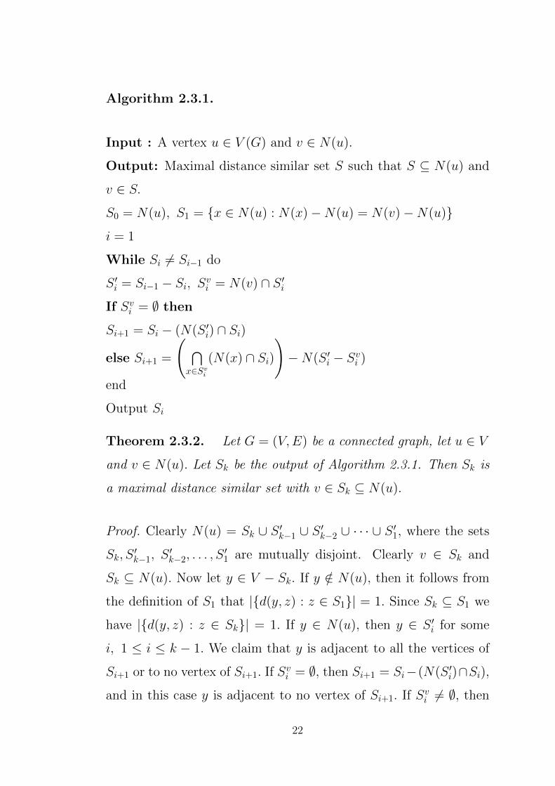
Algorithm 2.3.1.

Input : A vertex u ∈ V (G) and v ∈ N(u).

Output: Maximal distance similar set S such that S ⊆ N(u) and

v ∈ S.

S0 = N(u), S1 = x ∈ N(u) : N(x)−N(u) = N(v)−N(u)

i = 1

While Si 6= Si−1 do

S ′i = Si−1 − Si, Svi = N(v) ∩ S ′i

If Svi = ∅ then

Si+1 = Si − (N(S ′i) ∩ Si)

else Si+1 =

( ⋂x∈Sv

i

(N(x) ∩ Si)

)−N(S ′i − Sv

i )

end

Output Si

Theorem 2.3.2. Let G = (V,E) be a connected graph, let u ∈ V

and v ∈ N(u). Let Sk be the output of Algorithm 2.3.1. Then Sk is

a maximal distance similar set with v ∈ Sk ⊆ N(u).

Proof. Clearly N(u) = Sk ∪ S ′k−1 ∪ S ′k−2 ∪ · · · ∪ S ′1, where the sets

Sk, S′k−1, S

′k−2, . . . , S

′1 are mutually disjoint. Clearly v ∈ Sk and

Sk ⊆ N(u). Now let y ∈ V − Sk. If y /∈ N(u), then it follows from

the definition of S1 that |d(y, z) : z ∈ S1| = 1. Since Sk ⊆ S1 we

have |d(y, z) : z ∈ Sk| = 1. If y ∈ N(u), then y ∈ S ′i for some

i, 1 ≤ i ≤ k − 1. We claim that y is adjacent to all the vertices of

Si+1 or to no vertex of Si+1. If Svi = ∅, then Si+1 = Si−(N(S ′i)∩Si),

and in this case y is adjacent to no vertex of Si+1. If Svi 6= ∅, then

22

Si+1 =

( ⋂x∈Sv

i

(N(x) ∩ Si)

)−N(S ′i−Sv

i ). If y ∈ Svi , then y is adjacent

to all the vertices of Si+1, and if y ∈ Si − Svi , then y is adjacent to

no vertex of Si+1. Since y ∈ N(u), it follows that either d(y, z) = 1

for all z ∈ Si+1 or d(y, z) = 2 for all z ∈ Si+1. Also Sk ⊆ Si+1 and

hence |d(y, z) : z ∈ Sk| = 1. Thus Sk is a distance similar set of

G.

Now let S be any distance similar set in G such that v ∈

S ⊆ N(u). We claim that S ⊆ Sk. Suppose there exists a vertex

y such that y ∈ S and y /∈ Sk. Hence y ∈ S ′i for some i, 1 ≤

i ≤ k − 1. If Svi = ∅, then S ′i = N(S ′i−1) ∩ Si−1. Since y ∈ S ′i,

there exists z ∈ S ′i−1 such that zy ∈ E(G). Also zv /∈ E(G), and

both y, v ∈ S, which is a contradiction. If Svi 6= ∅, then S ′i =

Si−1−

(( ⋂x∈Sv

i−1

(N(x) ∩ Si−1)

)−N(S ′i−1 − Sv

i−1)

). If y ∈ N(S ′i−1−

Svi−1), then there exists z ∈ S ′i−1 − Sv

i−1 such that zy ∈ E(G). Also

zv /∈ E(G) and both z, v ∈ S, which is a contradiction. If y /∈( ⋂x∈Sv

i−1

(N(x) ∩ Si−1)

), then there exists y1 ∈ Sv

i−1 such that yy1 /∈

E(G). Also y1v ∈ E(G), which is a contradiction. Therefore S ⊆ Sk.

Thus Sk is a maximal distance similar set with v ∈ Sk ⊆ N(u).

Illustration 2.3.3. We illustrate Algorithm 2.3.1 with an exam-

ple. For the graph G3 given in Figure 2.3, we find the maximal dis-

tance similar set S such that S ⊆ N(u) and v ∈ S. From Algorithm

2.3.1, we have S0 = v, v1, v2, v3, v4, S1 = v, v1, v2, S ′1 = v3, v4

and Sv1 = ∅. Since Sv

1 = ∅, S2 = v, v1, S ′2 = v2 and Sv2 = ∅. Since

Sv2 = ∅, S3 = S2−(N(S ′2)∩S2) = S2−∅ = S2. Therefore S3 = v, v1

23

is the output of Algorithm 2.3.1 and is a maximal distance similar

set containing v.

r rr r

rr

rr

u

v

v1

v2

v5 v6

v3

v4

G3

Figure 2.3: Example for illustration of Algorithm 2.3.1.

Theorem 2.3.4. For any graph G, ds(G) can be computed in

O(n4) time.

Proof. Let u ∈ V (G) and let v ∈ N(u). Let f(u) = max|S| : S is a

maximal distance similar set and S ⊆ N(u). Given the adjacency

list of the graph G, the sets S0, S1, S′

i and Svi in Algorithm 2.3.1

can be determined in O(n) time each. Also the set Si+1 can be

determined in O(n2) time both when Svi = ∅ and Sv

i 6= ∅. Since the

while loop is executed at most n times, it follows that the algorithm

takes O(n3) time to find the maximal distance similar set S ⊆ N(u)

containing v. Hence f(u) can be computed in O(n3) time. Now,

since ds(G) = maxf(u) : u ∈ V (G), it follows that ds(G) can be

computed in O(n4) time.

24

2.4 GRAPHS WITH ds(G) = 1

In this section we present several families of graphs with

ds(G) = 1.

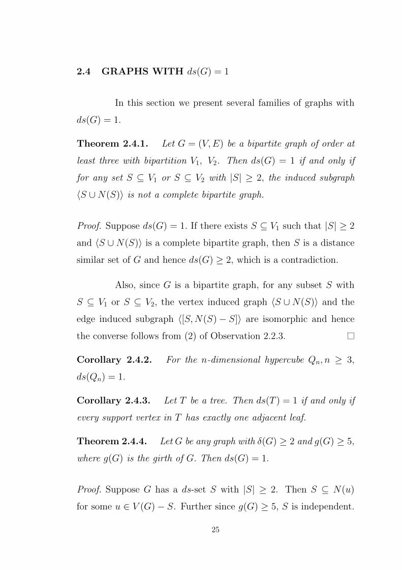
Theorem 2.4.1. Let G = (V,E) be a bipartite graph of order at

least three with bipartition V1, V2. Then ds(G) = 1 if and only if

for any set S ⊆ V1 or S ⊆ V2 with |S| ≥ 2, the induced subgraph

〈S ∪N(S)〉 is not a complete bipartite graph.

Proof. Suppose ds(G) = 1. If there exists S ⊆ V1 such that |S| ≥ 2

and 〈S ∪N(S)〉 is a complete bipartite graph, then S is a distance

similar set of G and hence ds(G) ≥ 2, which is a contradiction.

Also, since G is a bipartite graph, for any subset S with

S ⊆ V1 or S ⊆ V2, the vertex induced graph 〈S ∪N(S)〉 and the

edge induced subgraph 〈[S,N(S)− S]〉 are isomorphic and hence

the converse follows from (2) of Observation 2.2.3.

Corollary 2.4.2. For the n-dimensional hypercube Qn, n ≥ 3,

ds(Qn) = 1.

Corollary 2.4.3. Let T be a tree. Then ds(T ) = 1 if and only if

every support vertex in T has exactly one adjacent leaf.

Theorem 2.4.4. Let G be any graph with δ(G) ≥ 2 and g(G) ≥ 5,

where g(G) is the girth of G. Then ds(G) = 1.

Proof. Suppose G has a ds-set S with |S| ≥ 2. Then S ⊆ N(u)

for some u ∈ V (G)− S. Further since g(G) ≥ 5, S is independent.

25

Now, since δ(G) ≥ 2, there exists a vertex v ∈ N(S) − S with

v 6= u and both u and v are adjacent to all the vertices in S. Thus

G contains a cycle C4, a contradiction. Hence ds(G) = 1.

Theorem 2.4.5. Let G be a unicyclic graph with cycle C. Then

ds(G) = 1 if and only if G satisfies the following:

(i) Every support vertex in G has exactly one adjacent leaf.

(ii) If C = C3, then at most one vertex of C3 has degree two and if

C = C4, then at most two vertices of C4 have degree two and

they are adjacent.

Proof. Suppose ds(G) = 1. Since the set of all leaves adjacent to

any support vertex of G forms a distance similar set, (i) follows.

If G does not satisfy (ii), then the two vertices in C3 with degree

two or the two nonadjacent vertices in C4 with degree two form a

distance similar set of G, a contradiction. Therefore G satisfies the

conditions (i) and (ii).

Conversely, let G be a unicyclic graph satisfying the con-

ditions (i) and (ii). Suppose ds(G) ≥ 2 and let S be any ds-set of G.

Since |S| ≥ 2 and any two vertices of S lie on a cycle, it follows that

S ⊆ V (C). Further S is a ds-set of the cycle C and since ds(Cn) = 1

if n ≥ 5, it follows that C = C3 or C = C4. Now condition (ii) im-

plies that 〈[S,N(S)− S]〉 is not a complete bipartite graph, which

is a contradiction. Thus ds(G) = 1.

26

2.5 DISTANCE SIMILAR SETS AND RESOLVING SETS

In Proposition 2.1.1, Saenpolphat and Zhang presented a

lower bound for metric dimension of a graph in terms of order and

number of equivalence classes of a graph. In this section we obtain

a sharp and better lower bound for the metric dimension of a graph

G by using maximal distance similar sets of G.

Theorem 2.5.1. Let S be any maximal distance similar set in G

with |S| ≥ 2 and let S ⊆ N(u). Then dim(G) ≥ dim(〈S ∪ u〉)−1.

Proof. Let W be a basis of G. Let v1, v2 ∈ S. If W ∩ S = ∅, then

r(v1|W ) = r(v2|W ). Hence it follows that W ∩ S 6= ∅ and any pair

of vertices in S is resolved by a vertex in W ∩ S. Hence W ∩ S or

(W∩S)∪u is a resolving set of 〈S ∪ u〉, so that dim(〈S ∪ u〉) ≤

|W ∩ S| + 1. Now, let T be any basis for 〈S ∪ u〉 . Then

W1 = (W − (W ∩ S)) ∪ (T ∩ S) is a resolving set of G and hence

|T ∩ S| ≥ |W ∩ S|. Thus dim(〈S ∪ u〉) ≥ |W ∩ S| and hence

dim(〈S ∪ u〉) = |W ∩ S| or |W ∩ S| + 1. Now dim(G) = |W | ≥

|W ∩ S| ≥ dim(〈S ∪ u〉)− 1.

Corollary 2.5.2. Let S1, S2, . . . , Sk be disjoint maximal distance

similar sets of G with |Si| ≥ 2. Then

dim(G) ≥k∑

i=1

(dim(〈Si〉+K1)− 1).

27

Corollary 2.5.3. Let S1, S2, . . . , Sk be disjoint maximal distance

similar sets of G with |Si| ≥ 2 and each Si is an independent set or

a clique. Then dim(G) ≥k∑

i=1

(|Si| − 1).

Observation 2.5.4. The lower bound for dim(G) given in

Corollary 2.5.2 is sharp. Consider the graph G obtained from the

star K1,k and k copies G1, G2, . . . , Gk of the path P3, where Gi =

(xi, yi, zi), by joining all the pendent vertices of the star to all the

vertices of each Gi. Then V (Gi), 1 ≤ i ≤ k, are maximal distance

similar sets of G and dim(〈V (Gi) ∪ ui〉) = 2 where ui is a pendent

vertex of the star K1,k. Further W = x1, x2, . . . , xk is a basis of G

and hence dim(G) = k =k∑

i=1

(dim(〈V (Gi) ∪ ui〉)− 1). Further for

any distance similar equivalence class Si in G, we have |Si| = 1 and

hence the bound for dim(G) given in Proposition 2.1.1 reduces to

the trivial inequality dim(G) ≥ 0. This shows that the bound given

in Theorem 2.5.1 is better than the one given in Proposition 2.1.1.

2.6 BOUNDS FOR DISTANCE SIMILAR NUMBER

Since ds(G) ≤ ∆(G) ≤ n − 1 and ds(G) = n − 1 if and

only if ∆(G) = n− 1, it follows that ds(G) ≤ n− 2 for any graph G

with ∆(G) 6= n− 1. The following theorem gives a characterization

of all graphs with ds(G) = ∆(G).

Theorem 2.6.1. Let G be any connected graph of order n. Then

ds(G) = ∆(G) if and only if ∆(G) ≥⌈n2

⌉and G = G1 + Kn−∆(G),

where G1 is any graph of order ∆(G).

28

Proof. Suppose ds(G) = ∆(G). Let S be a ds-set of G. Then S =

N(u) where u ∈ V (G) − S and d(u) = ∆(G). Now let v ∈ V − S

and let d(v, S) = t. Let P = (v = v0, v1, v2, . . . , vt) where vt ∈ S

be a shortest path. Now vt−1 is adjacent to vt in S and since S is

a ds-set, vt−1 is adjacent to all vertices in S. Thus d(vt−1) = ∆(G)

and t = 1. Thus every vertex in V − S is adjacent to every vertex

in S and V − S is an independent set in G. Hence G is isomorphic

to 〈S〉+Kn−∆(G). Further S and V − S are distance similar sets in

G and hence ∆(G) ≥ |V − S|, so that ∆(G) ≥⌈n2

⌉.

Conversely, suppose G is isomorphic to G1 + Kn−∆(G),

|V (G1)| = ∆(G) and ∆(G) ≥⌈n2

⌉. Then V (G1) is a distance sim-

ilar set of G with |V (G1)| = ∆(G). Hence it follows from (1) of

Observation 2.2.3 that ds(G) = ∆(G).

We now proceed to characterize graphs G with ds(G) =

n− 2, n− 3 and d(G).

Theorem 2.6.2. Let G be any graph of order n with n ≥ 5. Then

ds(G) = n− 2 if and only if G is isomorphic to 2K1 +H where H

is any graph of order n− 2 with ∆(H) < n− 3.

Proof. Suppose ds(G) = n − 2. Then ∆(G) = n − 2 by (1) of

Observation 2.2.3. Thus ds(G) = ∆(G) and the result follows from

Theorem 2.6.1.

Theorem 2.6.3. Let G be a graph of order n with n ≥ 6. Then

ds(G) = n− 3 if and only if G is isomorphic to one of the following

graphs.

29

(i) The graph obtained from any graph H of order n − 3 and the

path P3 by joining exactly one pendent vertex of P3 to all the

vertices of H.

(ii) The graph obtained from any graph H of order n−3 and K2∪K1

by joining exactly one vertex of K2 and the vertex of K1 to all

the vertices of H.

(iii) The graph H+ 3K1 or H+ (K2∪K1), where H is any graph of

order n− 3 with ∆(H) ≤ n− 5 and H does not contain K2,n−5

as a subgraph when ∆(G) = n− 2.

Proof. Let G be any connected graph of order n ≥ 6 with ds(G) =

n− 3. It follows from Observation 2.2.3 that n− 3 ≤ ∆(G) ≤ n− 2.

Now let S be a ds-set of G. Let u ∈ V − S be such that S ⊆ N(u)

and let V − S = u, v, w.

Case 1. ∆(G) = n− 3.

Then it follows from Theorem 2.6.1 that G = H + 3K1

where H is any graph of order n− 3. Hence G is isomorphic to the

graph given in (iii).

Case 2. ∆(G) = n− 2.

In this case the vertex u is adjacent to at most one of the

vertices v, w and hence 〈u, v, w〉 ∼= K3 or P3 or K2 ∪K1. Suppose

〈u, v, w〉 ∼= K3. Since G is connected, the vertices v and w are

adjacent to all the vertices of S. Also, if 〈S〉 contains a subgraph

K2,n−5 and V1 is a partite set of K2,n−5 with |V1| = n − 5, then

30

V1∪ (V −S) is a distance similar set of G of cardinality n−2, which

is a contradiction. Hence G is isomorphic to the graph given in (iii).

If 〈u, v, w〉 ∼= P3 = (u, v, w), then v is nonadjacent to the vertices

of S since ∆(G) = n − 2. Also if w is adjacent to all the vertices

of S, then S ∪ v is a distance similar set of cardinality n − 2, a

contradiction. Hence G is isomorphic to the graph given in (i). Now

we assume that 〈u, v, w〉 ∼= K2∪K1. Without loss of generality let

K2∪K1 = (u, v)∪w. Since G is connected, w is adjacent to all the

vertices of S. Now v is either adjacent to u only or adjacent to all

the vertices of S. If v is adjacent to u only, then G is isomorphic to

the graph given in (ii). Now suppose v is adjacent to all the vertices

of S. If 〈S〉 contains a subgraph K2,n−5 and V1 is a partite set of

K2,n−5 with |V1| = n − 5, then V1 ∪ (V − S) is a distance similar

set of G of cardinality n − 2, which is a contradiction. Hence G is

isomorphic to the graph given in (iii).

Conversely, let G be a graph as given in the theorem.

It follows from (1) of Observation 2.2.3 and Theorem 2.6.2 that

ds(G) ≤ n− 3. Further V (H) is a ds-set of G of cardinality n− 3.

Thus ds(G) = n− 3.

Theorem 2.6.4. Let G be any graph of order n ≥ 4 and diameter

d. Then the following holds:

(i) If d ≥ 3, then ds(G) ≤ n− d and ds(G) = n− d if and only if

G can be obtained from a path P of length d by replacing any

vertex vi of P by any graph H of order ds(G) and joining every

vertex of H to the neighbors of vi in P .

31

(ii) If d = 2 and ∆(G) < n− 1, then ds(G) ≤ n− d and ds(G) =

n − d if and only if G = H + 2K1 where H is any graph of

order n− 2 with ∆(H) < n− 3.

(iii) If d = 1, then ds(G) = n− d.

Proof. (i) Let S be a ds-set of G. Then S ⊆ N(u) for all u ∈

N(S)− S. Let P be a diametrical path in G. Since d ≥ 3, we have

|V (P ) ∩ S| ≤ 1. Hence |V (P )| = d + 1 ≤ n − ds(G) + 1. Thus

ds(G) ≤ n− d.

Now let G be any graph with d ≥ 3 and let ds(G) = n−d.

Let S be a ds-set of G with |S| = n−d. Let P = (v1, v2, . . . , vd+1) be

a diametrical path in G. Since |S| = n−d, V (P )∩S 6= ∅. Let vi ∈ S.

Since S is a ds-set of G, it follows that the vertices in N(vi) ∩ P

are adjacent to all the vertices of S. Hence G is isomorphic to the

graph given in the theorem with H = 〈S〉 .

The converse is obvious.

(ii) Suppose d = 2 and ∆(G) < n−1. It follows from (1) of

Observation 2.2.3 that ds(G) ≤ n − 2. Also it follows from

Theorem 2.6.2 that ds(G) = n − 2 if and only if G = H + 2K1

where H is any graph of order n− 2 with ∆(H) < n− 3.

(iii) If d = 1, then G = Kn and hence ds(G) = n− 1.

32

2.7 DISTANCE SIMILAR SETS AND GRAPH

OPERATIONS

In this section we determine the distance similar number

of a graph which is obtained by applying graph operations on two

graphs.

Theorem 2.7.1. Let G and H be any two nontrivial connected

graphs of order n1 and n2 respectively. Then

ds(GH) =

2 if G = H = K2

1 otherwise.

Proof. If G = H = K2, then ds(GH) = ds(C4) = 2. Suppose

G 6= K2. Let G1, G2, . . . , Gn2be the copies of G in GH. Suppose

there exists a distance similar set S of GH with |S| ≥ 2 and let

S ⊆ N(u). If |V (Gi) ∩ S| ≥ 2 for some i, 1 ≤ i ≤ n2, then u =

(vi, ut) ∈ V (Gi). Now let x, y ∈ V (Gi) ∩ S and let x = (vi, uk), y =

(vi, ul). Let vj ∈ NG(vi). Then x′ = (vj, uk) /∈ S, d(x′, x) = 1 and

d(x′, y) ≥ 2, which is a contradiction. Hence |V (Gi) ∩ S| ≤ 1 for

each i, 1 ≤ i ≤ n2. Now since |S| ≥ 2, we have |V (Gi) ∩ S| =

|V (Gj) ∩ S| = 1 for some i, j with i 6= j. Let V (Gi) ∩ S = x and

V (Gj) ∩ S = y. Hence x = (vi, uk) and y = (vj, ul) for some k, l

with 1 ≤ k ≤ l ≤ n2. If k = l, then for any z ∈ V (Gi) ∩ N(x), we

have d(z, x) = 1 and d(z, y) ≥ 2, a contradiction.

If k 6= l, then u = (vi, ul) or u = (vj, uk). We assume that

u = (vi, ul). Since G 6= K2, there exists z = (vi, um) ∈ V (Gi) such

that either uz ∈ E(GH) or xz ∈ E(GH). If xz ∈ E(GH), we

33

have d(z, x) = 1 and d(z, y) ≥ 2. If uz ∈ E(GH), then d(z′, y) = 1

and d(z′, x) ≥ 2, where z′ = (vj, um). Thus in all cases we get a

contradiction. Hence ds(GH) = 1.

Theorem 2.7.2. Let G be any connected graph and let H be any

graph. Then ds(G H) = |V (H)|.

Proof. Let V (G) = v1, v2, . . . , vn. Let H1, H2, . . . , Hn be the copies

of H such that vi is adjacent to each vertex in Hi, 1 ≤ i ≤ n. If S

is any ds-set of G H, then either S = vi or S ⊆ V (Hi). Thus

ds(G H) = |S| ≤ |V (H)|. Further V (Hi) is a maximal distance

similar set ofGH and hence it follows that ds(GH) = |V (H)|.


graphs of order n1 and n2 respectively. Then maxn1, n2 ≤ ds(G+

H) ≤ maxn1 + ds(H), n2 + ds(G).

Proof. Let V (G) = v1, v2, . . . , vn1 and V (H) = u1, u2, . . . , un2

.

Clearly V (G) and V (H) are distance similar sets of G + H and

hence ds(G + H) ≥ maxn1, n2. Now let S be a ds-set of G + H.

Then S ⊆ N(w) for some w ∈ V (G + H). If w = vi ∈ V (G) for

some i, then V (H) ⊆ S. Let vj ∈ V (G) − S. Since d(vj, ui) = 1

for all ui ∈ V (H), d(vj, vk) = 1 for all vk ∈ V (G) ∩ S. Hence

G = 〈V (G) ∩ S〉 + 〈V (G)− S〉 and |V (G) ∩ S| ≤ ds(G). Thus

|S| ≤ n2+ds(G). Similarly |S| ≤ n1+ds(H) and hence ds(G+H) ≤

maxn1 + ds(H), n2 + ds(G).

34

Observation 2.7.4. The bounds given in Theorem 2.7.3 are

sharp. If G1 = P5, and H1 = P4, then V (G1) and V (H1) are the only

maximal distance similar sets of G1 +H1, and hence ds(G1 +H1) =

5 = max|V (G1)|, |V (H1)|. If G2 = K3,3 with bipartition V1, V2

and H2 = P5, then V1 ∪ V (H2) and V2 ∪ V (H2) are the maxi-

mal distance similar sets of G2 + H2. Hence ds(G2 + H2) = 8 =

max|V (G2)|+ ds(H2), |V (H2)|+ ds(G2).

Observation 2.7.5.

(1) Let G = G1 + G2 + · · · + Gk be the sequential join of graphs

G1, G2, . . . , Gk of orders n1, n2, . . . , nk respectively and k ≥ 4.

Then V (G1), V (G2), . . . , V (Gk) are the only maximal distance

similar sets of G and hence ds(G) = maxn1, n2, . . . , nk.

(2) Let G = G1 +G2 +G3 be the sequential join of graphs G1, G2

and G3 of order n1, n2 and n3 respectively. Then V (G2) and

V (G1)∪V (G3) are the only maximal distance similar sets of G

hence ds(G) = maxn2, n1 + n3.


graphs of order n1 and n2 respectively. Then

ds(G∗H) =

ds(G)n2 + ds(H) if ∆(G) = n1 − 1

and there exists a ds-set S2 of H

such that H = 〈S2〉+ 〈V (H)− S2〉

ds(G)n2 otherwise.


.

Let Hi = 〈(vi, uj) : 1 ≤ j ≤ n2〉 be the copies of H in G ∗ H

35

corresponding to vi. Then for any two distinct vertices (vi, ur), (vj, us)

in G ∗H, we have

dG∗H((vi, ur), (vj, us)) =

dG(vi, vj) if i 6= j

1 if i = j and urus ∈ E(H)

2 otherwise.

Hence if S is a ds-set of G, then S ′ =⋃vi∈S

V (Hi) is a distance

similar set of G ∗H. Hence ds(G ∗H) ≥ |S ′| = ds(G)n2. Now sup-

pose ds(G ∗ H) > ds(G)n2. Let S1 be any ds-set of G ∗ H and let

S1 ⊆ NG∗H((vi, ur)). Let T = vj : V (Hj) ∩ S1 6= ∅ and j 6= i.

Then T is a distance similar set of G and hence |T | ≤ ds(G). If

|T | < ds(G), then |S1| < ds(G)n2, which is a contradiction. Hence

|T | = ds(G) and⋃

vj∈TV (Hj) ⊆ S1. Since |S1| > ds(G)n2, it follows

that V (Hi) ∩ S1 6= ∅.

We now claim that dG(vi) = n1−1. If not, let vl ∈ V (G) be

such that dG(vi, vl) = 2. Let (vi, vk, vl) be an induced path in G. If

V (Hk) ⊆ S1, then d((vl, us), (vk, ur)) = 1, and d((vl, us), (vi, us)) = 2

for all (vi, us) ∈ V (Hi) ∩ S1, which is a contradiction. Suppose

V (Hk) * S1. Then V (Hk) ∩ S1 = ∅. Now for any x = (vk, us) ∈

V (Hk), d(x,w) = 1 for all w ∈ V (Hi) ∩ S1 and hence d(x,w) = 1

for all w ∈ S1. Thus

( ⋃vj∈T

V (Hj)

)∪ V (Hi) ⊆ NG∗H((vk, us)) is a

distance similar set in G∗H and hence T ∪vi is a distance similar

set in G, of cardinality ds(G) + 1, which is a contradiction. Thus

dG(vi) = n1 − 1.

36

Now let (vi, ur) ∈ V (Hi) − S1. Since d((vi, ur), (vj, us)) = 1 for all

vj ∈ T and s = 1, 2, . . . , n2, it follows that

d((vi, ur)(vi, us)) = 1 for all (vi, us) ∈ V (Hi) ∩ S1.

Hence H = 〈V (Hi) ∩ S1〉+ 〈V (Hi)− S1〉 and |V (Hi)∩S1| = ds(H).

Conversely, assume that ∆(G) = n1 − 1 and H = 〈S2〉 +

〈V (H)− S2〉 where S2 is a ds-set of H. Let vi ∈ V (G) be such

that dG(vi) = n1 − 1 and let Si2 = (vi, uk) : uk ∈ S2. Then(

n1⋃j=1, j 6=i

V (Hj)

)∪(V (Hi)∩Si

2) is a distance similar set of maximum

order and ds(G ∗H) = (n1− 1)n2 + ds(H) = ds(G)n2 + ds(H).

Now we present a theorem which gives the distance similar

number of trestled graph Tk(G) of G of index k where k is any

positive integer.

Theorem 2.7.7. Let G be a nontrivial connected graph. Then

ds(Tk(G)) =

1 if δ(G) ≥ 2 or k ≥ 2

2 if δ(G) = k = 1.

Proof. Let V (G) = v1, v2, . . . , vn and E(G) = e1, e2, . . . , em.

Let e1i = v1

sv1t , e

2i = v2

sv2t , . . . , e

ki = vksv

kt be the edges of Tk(G)

corresponding to the edge ei = vsvt ∈ E(G), 1 ≤ i ≤ m. First

we prove that ds(Tk(G)) ≤ 2. Let S be a ds-set of Tk(G). Then

there exists u ∈ V (Tk(G)) such that S ⊆ N(u). If S contains

two distinct vertices of G say vi, vj, then u ∈ V (G). In this case

for any vertex vri in V (Tk(G)) − V (G) which is adjacent to vi,

we have vri /∈ S, d(vri , vi) = 1 and d(vri , vj) ≥ 2, a contradiction.

37

Thus |V (G) ∩ S| ≤ 1. If S contains two distinct vertices x, y of

V (Tk(G)) − V (G), then u = vl for some vl ∈ V (G), and x = vrl

where 1 ≤ r ≤ k. Now d(vrt , vrl ) = 1 and d(vrt , y) ≥ 3, a contradic-

tion. Thus |(V (Tk(G)) − V (G)) ∩ S| ≤ 1. Hence |S| ≤ 2, so that

ds(Tk(G)) ≤ 2. Also if |S| = 2, we may assume that S = vi, v1p

where vivp ∈ E(G). However such a set S is not a distance sim-

ilar set of Tk(G) if either δ(G) ≥ 2 or k ≥ 2. Hence in this case

ds(Tk(G)) = 1.

Now if δ(G) = k = 1, then S = v1i , vj where vj is a

pendent vertex of G and vivj ∈ E(G), is a maximal distance similar

set of Tk(G). Hence ds(Tk(G)) = 2.

2.8 CONCLUSION AND SCOPE

Motivated by the concept of distance similarity we have

introduced distance similar set and distance similar number of a

graph. We have presented several basic results on this new pa-

rameter. The following are some interesting problems for further

investigation.

Problem 2.8.1. Characterize all graphs having a disjoint collec-

tion S1, S2, . . . , Sk of distance similar sets with |Si| ≥ 2 such that

dim(G) =k∑

i=1

(dim(〈Si〉+K1)− 1).

Problem 2.8.2. Determine the distance similar number of other

families of graphs such as split graphs, chordal graphs, comparability

graphs and interval graphs.

38

CHAPTER 3

PAIRWISE DISTANCE SIMILAR SETS IN

GRAPHS∗

3.1 INTRODUCTION

In this chapter we initiate a study of pairwise distance

similar number of a graph, which arises naturally from the concept

of distance similar equivalence class. Two vertices u and v of a

connected graph G are distance similar if d(u, x) = d(v, x) for all

x ∈ V (G)− u, v.

We observe that u and v are distance similar vertices if and

only if N(u) = N(v) if uv /∈ E(G) and N [u] = N [v] if uv ∈ E(G).

Hernando et al. [18] called a pair of vertices satisfying the above

equivalent condition as twins and introduced the concept of the twin

graph of a graph G. The relation ≡ on V (G) defined by u ≡ v if and

only if u = v or u, v are twins is an equivalence relation on V (G).

For each vertex v ∈ V (G), let v∗ be the set of vertices of G that

are equivalent to v under ≡ . Let v∗1, v∗2, . . . , v∗k be the partition

of V (G) induced by ≡ . Each v∗i is either independent or 〈v∗i 〉 is a

∗The content of this chapter has been published in J. Combin. Math. Combin. Comput.,84 (2013), 21–28.

complete graph in G. Further⟨[v∗i , v

∗j ]⟩

is a complete bipartite graph

if vivj ∈ E(G) and is an empty graph if vivj /∈ E(G). The twin

graph of G, denoted by G∗, is the graph with vertex set V (G∗) =

v∗1, v∗2, . . . , v∗k, and v∗i v∗j ∈ E(G∗) if and only if vivj ∈ E(G). We

observe that each equivalence class v∗i has the property that any two

vertices of v∗i are distance similar and v∗i is maximal with respect to

this property.

In this chapter we introduce pairwise distance similar

number Φ(G) and lower pairwise distance similar number Φ−(G)

for any connected graph and present several basic results on these

parameters.

3.2 BASIC RESULTS

Definition 3.2.1. Let G = (V,E) be a connected graph. A

nonempty subset S of V is called a pairwise distance similar set

(pds-set) if either |S| = 1 or any two vertices in S are distance

similar. The maximum cardinality of a maximal pds-set in G is

called the pairwise distance similar number of G and is denoted by

Φ(G). The minimum cardinality of a maximal pds-set in G is called

the lower pairwise distance similar number of G and is denoted by

Φ−(G). Any maximal pds-set with |S| = Φ(G) is called a Φ-set

of G.

40

Clearly the equivalence classes v∗1, v∗2, . . . , v

∗k with respect to

the distance similarly relation ≡ are precisely the set of all maximal

pds-sets of a graph G. Also G = G0[〈v∗1〉, 〈v∗2〉, . . . , 〈v∗k〉] where G0 is

the graph obtained from G by contracting each equivalence class v∗i

as a single vertex. The graph G0 is called the twin graph of G. Hence

Φ(G) = max1≤i≤k

|v∗i | and Φ−(G) = min1≤i≤k

|v∗i |. Hence it follows that both

Φ(G) and Φ−(G) can be computed with complexity O(n2).

Example 3.2.2. For the graph G1 given in Figure 3.1, v∗1 =

v1, v∗2 = v2, v5, v6, v7, v∗3 = v3 and v∗4 = v4 are the maximal

pds-sets. Hence Φ−(G1) = 1 and Φ(G1) = 4. The twin graph G∗1 is

P4 and G1 = G∗1[K1, K4, K1, K1].

rrrr

r rrv1

v2

v5

v6

v7

v3 v4

G1

Figure 3.1: Graph with Φ = 4 and Φ− = 1.

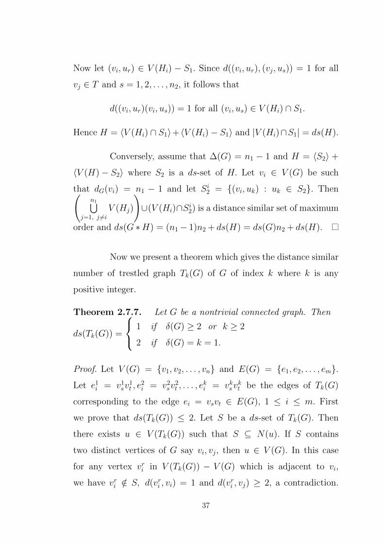
Example 3.2.3. For the graph G2 given in Figure 3.2, V1 =

v1, v2, v3, V2 = v4, v5, V3 = v6, v7 and V4 = v8, v9 are

maximal pds-sets. Also, Φ−(G2) = 2 and Φ(G2) = 3. The twin

graph G∗2 = P4 and G2 = G∗2[K3, K2, K2, K2]. For the graph G3

given in Figure 3.2, v1, v2, v3, v4 and v5, v6 are maximal pds-

sets. Hence Φ−(G3) = Φ(G3) = 2. Also G∗3 = P3 and G3 =

G∗3[K2, K2, K2].

41

rrrr r

rr

rr

v1

v2

v3

v4 v6 v8

v5 v7 v9

rr

rr

rr

v1 v3 v5

v2 v4 v6G2 G3

Figure 3.2: Graphs with unequal and equal Φ and Φ−.

The following are some immediate observations of the

pairwise and lower pairwise distance similar number of a graph.

Observation 3.2.4.

(1) If a proper subset S of V (G) is a pds-set of G, then the edge

induced subgraph of [S,N(S)−S] is a complete bipartite graph.

(2) Let G be any connected graph of order n which is not complete.

Then there exist at least two disjoint maximal pds-sets in V (G)

and hence Φ−(G) ≤⌊n2

⌋.

(3) Let G be any connected graph. Then Φ(G) = 1 if and only if

|v∗i | = 1 for each i and hence it follows that G = G∗.

(4) Let T be any tree. Then Φ(T ∗) = 1 where T ∗ is the twin graph

of T.

Lemma 3.2.5. Let S be a pds-set of G and S ( V (G). Then S

is a distance similar set of G.

Proof. Let S = v1, v2, . . . , vk be a pds-set of G. Let u ∈ V (G) −

S and d(u, v1) = t. Since v1 and vi are distance similar for all

i = 2, 3, . . . , k, we have d(u, vi) = t for all i = 2, 3, . . . , k. Hence

|d(u, vi) : vi ∈ S| = 1. Thus S is a distance similar set of G.

42

Corollary 3.2.6. Let G be any connected graph which is not com-

plete. Let S be any pds-set of G. Then S ⊆ N(u) for any vertex u

in N(S)− S. Hence 1 ≤ Φ−(G) ≤ Φ(G) ≤ ∆(G).

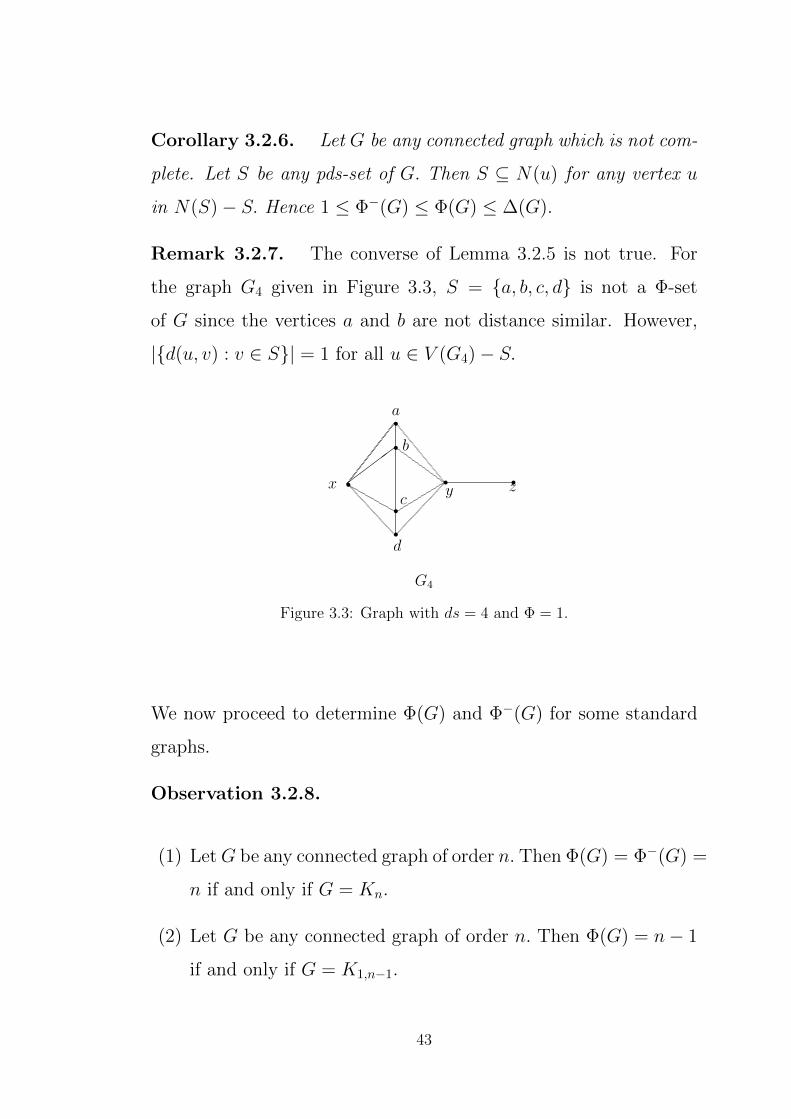
Remark 3.2.7. The converse of Lemma 3.2.5 is not true. For

the graph G4 given in Figure 3.3, S = a, b, c, d is not a Φ-set

of G since the vertices a and b are not distance similar. However,

|d(u, v) : v ∈ S| = 1 for all u ∈ V (G4)− S.

rrrr

r rr

a

b

c

d

x y z

G4

Figure 3.3: Graph with ds = 4 and Φ = 1.

We now proceed to determine Φ(G) and Φ−(G) for some standard

graphs.

Observation 3.2.8.

(1) LetG be any connected graph of order n. Then Φ(G) = Φ−(G) =

n if and only if G = Kn.

(2) Let G be any connected graph of order n. Then Φ(G) = n− 1

if and only if G = K1,n−1.

43

(3) For the cycle Cn, we have Φ(Cn) = Φ−(Cn) =

3 if n = 3

2 if n = 4

1 if n ≥ 5.

Theorem 3.2.9. Let G be any graph with δ(G) ≥ 2 and g(G) ≥ 5

where g(G) is the girth of G. Then Φ(G) = 1.

Proof. Suppose G has a Φ-set S with |S| ≥ 2. Then S ⊆ N(u) for

some u ∈ V (G)−S. Since g(G) ≥ 5, it follows that S is independent

and since δ(G) ≥ 2, there exists a vertex v ∈ N(S)− S with v 6= u.

Now, both u and v are adjacent to all the vertices in S. Thus G

contains a cycle C4, a contradiction. Hence Φ(G) = 1.

Theorem 3.2.10. Let T be any tree. For any vertex v of T,

let l(v) denote the number of leaves adjacent to v. Then Φ(T ) =

maxl(v) : v is a support vertex of T and Φ−(T ) = 1.

Proof. Suppose S = v1, v2, . . . , vk is a Φ-set of T with |S| ≥ 2 and

S ⊆ N(u) for some u ∈ V (T ). Since 〈S〉 is independent, 〈S ∪ u〉

is a star. Let w ∈ V (T )− (S∪u). If w is adjacent to some vi ∈ S,

then w is adjacent to all the vertices of S and hence 〈S ∪ u,w〉

contains a cycle, a contradiction. Therefore vi, i = 1, 2, . . . , k are

pendent vertices in T. Thus Φ(T ) = maxl(v) : v is a support vertex

of T. Further, if x is any support vertex in T, then x is a maximal

pds-set of T and hence Φ−(T ) = 1.

We now proceed to obtain a characterization of graphs

with Φ(G) = ∆(G), Φ−(G) = ∆(G), Φ(G) = n−2 and Φ(G) = n−3.

44

Theorem 3.2.11. Let G be a graph of order n with ∆(G) > 0.

Then Φ(G) = ∆(G) if and only if G is isomorphic to the complete

bipartite graph Kn1,n2where maxn1, n2 = ∆.

Proof. Let S be any Φ-set of G with |S| = ∆(G) and let S = N(u)

for some u ∈ V (G). If 〈S〉 is complete, then H = 〈S ∪ u〉 = K∆+1.

Hence it follows that G = H and Φ(G) = ∆(G)+1, a contradiction.

Hence 〈S〉 is independent. Now, let v ∈ V (G) − N [u]. If d(v, S) =

k ≥ 2, let P = (v, v1, . . . , vt) be a geodesic joining v and S. Then

vt−1 is adjacent to all the vertices of S and also to vt−2. Hence

deg(vt−1) ≥ ∆(G) + 1, a contradiction. Hence d(v, S) = 1 for all

v ∈ V (G) − N [u]. Also since deg(v) = ∆(G) for all v ∈ V (G) − S,

it follows that V (G)− S is independent. Hence G is isomorphic to

the complete bipartite graph with bipartition S, V (G)− S.


Corollary 3.2.12. For any graph G of order n, Φ−(G) = ∆(G)

if and only if n is even and G = Kn2 ,

n2.

Proof. If Φ−(G) = ∆(G), then Φ(G) = ∆(G). By Theorem 3.2.11,

we have ∆ = n−∆ and G = Kn2 ,

n2. The converse is obvious.

Theorem 3.2.13. Let G be any connected graph of order n ≥ 4.

Then Φ(G) = n−2 if and only if G is isomorphic to one of the graphs

P3[Kn−2, K1, K1], P2[Kn−2, 2K1], P2[Kn−2, 2K1], P2[Kn−2, K2].

Proof. Let S be any Φ-set of G with |S| = n− 2 and let S ⊆ N(u)

for some u ∈ V (G). Clearly G∗ = P3 or P2. If G∗ = P3, then

45

G = P3[Kn−2, K1, K1] and if G∗ = P2, then G = P2[Kn−2, K2] or

P2[Kn−2, 2K1] or P2[Kn−2, 2K1]. Hence it follows that G is isomor-

phic to one of the graphs given in the theorem.


Theorem 3.2.14. Let G be any connected graph of order n ≥ 6

and let H = Kn−3 or Kn−3. Then Φ(G) = n− 3 if and only if G is

isomorphic to one of the following graphs.

(i) P2[H, 3K1], P2[Kn−3, K3].

(ii) P3[K1, H,K2], P3[H,K2, K1], P3[H,K1, K2], P3[Kn−3, K1, 2K1],

P3[Kn−3, 2K1, K1], K3[Kn−3, 2K1, K1].

(iii) P4[H,K1, K1, K1], P4[K1, H,K1, K1], G1[Kn−3, K1, K1, K1] where

G1 is the graph given in Figure 3.4.

ss

s sv1

v2

v3 v4G1

Figure 3.4: Graph with Φ = n− 3.

Proof. Let S be any Φ-set of G with |S| = n − 3 and let G∗ be

the twin graph of G. Then 2 ≤ |V (G∗)| ≤ 4. If |V (G∗)| = 2, then

G is isomorphic to one of the graphs given in (i). If |V (G∗)| = 3

and G∗ = K3, then G = K3[Kn−3, 2K1, K1]. Now suppose G∗ =

P3 = (v∗1, v∗2, v∗3). We may assume without loss of generality that the

46

vertex v∗ of G∗ corresponding to S is either v∗1 or v∗2. If v = v∗2, then

G is isomorphic to P3[K1, H,K2]. If v∗ = v∗1, then G is isomorphic to

one of the graphs P3[H,K2, K1], P3[H,K1, K2], P3[Kn−3, K1, 2K1]

or P3[Kn−3, 2K1, K1].

Now, suppose |V (G∗)| = 4. Since there exist three single-

ton subsets of V (G) which are maximal pds-sets, G∗ is not isomor-

phic to K4−e, K1,3 or C4. Hence G∗ is isomorphic to P4 or K1,3 +e.

If G∗ = P4, then G = P4[H,K1, K1, K1] or P4[K1, H,K1, K1]. If

G∗ = K1,3 + e = G1, then G = G1[Kn−3, K1, K1, K1].


Theorem 3.2.15. Let Gi, 0 ≤ i ≤ n, be nontrivial connected

graphs with V (G0) = v1, v2, . . . , vn and let G = G0[G1, G2, . . . , Gn].

Let k = maxΦ(Gi) : 1 ≤ i ≤ n. Then k ≤ Φ(G) ≤ kΦ(G0) and

the bounds are sharp.

Proof. Clearly any Φ-set of Gi, 1 ≤ i ≤ n, is a pds-set of G and

hence it follows that Φ(G) ≥ k. Also if S is any Φ-set of G and

V (Gi)∩ S 6= ∅, then V (Gi)∩ S is a pds-set of Gi and vi ∈ V (G0) :

V (Gi) ∩ S 6= ∅ is a pds-set of G0. Hence Φ(G) ≤ kΦ(G0). The

upper bound is attained for the graph G = C4[K3, K4, K3, K4] and

the lower bound is attained for the graph G = P4[K4, K4, K4, K4].

Thus the bounds are sharp.

47

Corollary 3.2.16. Let G and H be any two nontrivial connected

graphs. Then maxΦ(G),Φ(H) ≤ Φ(G+H) ≤ Φ(G) + Φ(H).

Corollary 3.2.17. Let G = Pn[G1, G2, . . . , Gk], n ≥ 4 and each

Gi is a nontrivial graph. Then Φ(G) = maxΦ(Gi) : i = 1, 2, . . . , n.


In this chapter we have initiated a study of pds-set and the

two parameters Φ(G) and Φ−(G). The following are some interesting

problems for further investigation.

Problem 3.3.1. Characterize graphs G for which Φ−(G) = 1.

Problem 3.3.2. Characterize graphs G for which Φ(G) = 1.

Problem 3.3.3. For which graphs G and H, we have

(a) Φ(G+H) = maxΦ(G),Φ(H)

(b) Φ(G+H) = Φ(G) + Φ(H)?

48

CHAPTER 4

DISTANCE PATTERN DISTINGUISHING

SETS IN GRAPHS∗

4.1 INTRODUCTION

The concept of metric dimension was independently dis-

covered by Slater [29] and Harary and Melter [16]. By an ordered

set of vertices we mean a set W = w1, w2, · · · , wk on which the

ordering (w1, w2, · · · , wk) has been imposed. For an ordered subset

W = w1, w2, · · · , wk of V (G), we refer to the k-vector (ordered

k-tuple) r(v|W ) = (d(v, w1), d(v, w2), · · · , d(v, wk)) as the (metric)

representation of v with respect to W. The set W is called a resolv-

ing set for G if r(u|W ) = r(v|W ) implies u = v for all u, v ∈ V (G).

Hence if W is a resolving set of cardinality k for a graph G of order

n, then the set r(v|W ) : v ∈ V (G) consists of n distinct k-vectors.

A resolving set of minimum cardinality is called a basis for G and

the metric dimension of G is defined to be the cardinality of a basis

of G and is denoted by dim(G). Slater used the terms locating set

and locating number for resolving set and metric dimension.

∗A part of this chapter has been published in Adv. Stud. Contemp. Math. (Kyungshang),21 (2011), 107–114.

Applications of resolving sets arise in various areas

including coin weighing problem [28], drug discovery [10], robot

navigation [19], network discovery and verification [2], connected

joins in graphs [27] and strategies for the mastermind game [11].

For a survey of results in metric dimension we refer to Chartrand

and Ping [8].

In this chapter we introduce the concept of distance pat-

tern distinguishing sets (DPD-sets) in which a vertex v is repre-

sented by the set of all distances from v to the vertices of a fixed

set M and the DPD-number of G. We determine the DPD-number

of several families of graphs. We obtain a relation between DPD-

number and dim(G). Further we give some embedding techniques

to embed any graph into a DPD-graph. We define the concept

local distance pattern distinguishing set (LDPD-set) and LDPD-

number of a graph G. We obtain LDPD-number of several families

of graphs.

4.2 BASIC RESULTS

In this section we introduce the concept of DPD-set and

present several necessary conditions for a graph to admit a DPD-

set. We also obtain a few properties of DPD-set.

Definition 4.2.1. Let G = (V,E) be a connected graph and let

M ⊆ V. For each u ∈ V the set fM(u) = d(u, v) : v ∈M is called

the distance pattern of u with respect to the set M. If fM is injec-

tive, then the set M is called a distance pattern distinguishing set

50

(DPD-set) of G. If G admits a DPD-set, then G is called a DPD-

graph. The minimum cardinality of a DPD-set in a DPD-graph G

is the DPD-number of G and it is denoted by %(G).

Example 4.2.2. Consider the graph G given in Figure 4.1. Here

M = v1, v2, v3, v5, v6 is a DPD-set. We have fM(v1) = 0, 1, 2, 4,

fM(v2) = 0, 1, 3, fM(v3) = 0, 1, 2, fM(v4) = 1, 2, 3, fM(v5) =

0, 2, 3, 4 and fM(v6) = 0, 1, 2, 3.

s ss s ss

v1 v2 v3 v4 v5

v6

G

Figure 4.1: DPD-Graph.

Observation 4.2.3. For any graph G = (V,E) with |V | ≥ 2, V

is not a DPD-set, since for any two vertices u, v ∈ V with d(u, v) =

diam(G) we have fM(u) = fM(v) = 0, 1, 2, . . . , diam(G).

We observe that not every graph has a DPD-set as shown

in the following theorem.

Theorem 4.2.4. The complete graph Kn, n ≥ 3 does not possess

a DPD-set.

Proof. Let M be a nonempty subset of V (Kn). If M = u, then for

distinct vertices v and w different from u we have fM(v) = fM(w) =

1. If |M | ≥ 2, then for any two distinct vertices u, v ∈M we have

fM(u) = fM(v) = 0, 1. Hence M is not a DPD-set.

51

Theorem 4.2.5. For any connected graph G = (V,E), there ex-

ists no DPD-set of cardinality two.

Proof. Let M = x, y ⊆ V (G). Then fM(x) = fM(y) = 0, d(x, y)

and hence M is not a DPD-set.

Theorem 4.2.6. A graph G has a DPD-set of cardinality one if

and only if G is a path.

Proof. If G is a path say (u1, u2, . . . , un), then M = u1 is a DPD-

set of G. Conversely suppose G admits a DPD-set of cardinality

one, say x. Then the distance pattern of the n vertices of G are

0, 1, 2, . . . , n − 1. Hence there exists a vertex y in G such

that d(x, y) = n− 1 and hence it follows that G is a path.

Remark 4.2.7. A path may contain DPD-sets of cardinality

greater than one. For the path P5 = (v1, v2, v3, v4, v5) the sets M1 =

v1, v2, v4 and M2 = v1, v2, v3, v5 are DPD-sets.

Theorem 4.2.8. Let G be any graph having a DPD-set M. Then

any vertex of G is adjacent to at most two pendant vertices. Further,

if a vertex v is adjacent to two pendant vertices x, y, then exactly

one of the vertices x, y belongs to M.

Proof. Suppose that G has a vertex v which is adjacent to at least

three pendant vertices say x, y and z. Let M be any arbitrary subset

of V (G). Then either |M ∩x, y, z| ≥ 2 or |(V −M)∩x, y, z| ≥ 2

and in both cases the two vertices in M or (V −M) have the same

52

distance pattern. Hence M is not a DPD-set of G, which is a

contradiction. Hence v is adjacent to at most two pendant vertices.

Now, suppose v is adjacent to exactly two pendant vertices

say x, y. If x, y ⊆M or x, y∩M = ∅ then fM(x) = fM(y). Hence

exactly one of x, y must be in M.

The following result gives a necessary condition for a graph

to possess a unique DPD-set.

Theorem 4.2.9. If G is a graph having three pairwise distance

similar vertices x, y and z, then G is not a DPD-graph. Further if

G is a DPD-graph having exactly two distance similar vertices x, y

then exactly one of x, y lies in every DPD-set M of G.

Proof. Suppose G has three pairwise distance similar vertices x, y

and z. Let M ⊆ V (G). If |M∩x, y, z| ≥ 2, let x, y ∈M∩x, y, z.

Then fM(x) = fM(y). Also if |M ∩ x, y, z| ≤ 1, let x, y /∈ M ∩

x, y, z. Then fM(x) = fM(y). Hence G has no DPD-set. Now

let G be a DPD-graph having exactly two distance similar vertices

say x, y. Let M be a DPD-set of G. If x, y ∈ M or x, y /∈ M then

fM(x) = fM(y). Therefore exactly one of x, y belongs to M .

Corollary 4.2.10. Let G be a DPD-graph with δ(G) = 1. Then

any support of G is adjacent to at most two pendant vertices.

Theorem 4.2.11. If G is a DPD-graph with unique DPD-set

M, then G has no distance similar vertices.

53

Proof. Suppose there exist two distance similar vertices x, y ∈

V (G). By Theorem 4.2.9 exactly one of x, y in M . Suppose x ∈M ,

y /∈M . Then M1 = (M −x)∪ y is also a DPD-set of G which

is a contradiction.

Theorem 4.2.12. If a block G of order n ≥ 3 has a DPD-set

M, then G is not complete and 3 ≤ |M | ≤ n− 1.

Proof. Let G be a block of order n ≥ 3 having a DPD-set M. By

Theorem 4.2.4 G is not complete. By Theorem 4.2.6 and

Theorem 4.2.5, we have |M | ≥ 3. Also by Observation 4.2.3, |M | ≤

n− 1.

Theorem 4.2.13. A graph G of diameter two is a DPD-graph

if and only if G is isomorphic to P3.

Proof. If G is isomorphic to P3, then by Theorem 4.2.6 G is a DPD-

graph. Conversely, let G be any DPD-graph of diameter two with

DPD-set M. If G is not a path, then it follows from Theorem 4.2.6

and Theorem 4.2.5 that |M | ≥ 3. Let x, y, z ⊆M. Since diameter

of G is two, we may assume without loss of generality that fM(x) =

0, 1, fM(y) = 0, 2 and fM(z) = 0, 1, 2. Since fM(x) = 0, 1,

x is adjacent to both z and y. Hence 1 ∈ fM(y) which is a contra-

diction. Hence G is a path and since diam(G) = 2, G is isomorphic

to P3.

Theorem 4.2.14. Let G be any graph. Then the join G + G is

a DPD-graph if and only if G is isomorphic to K1.

54

Proof. If G is isomorphic to K1, then G + G is isomorphic to K2,

which is a DPD-graph. Conversely, suppose G + G is a DPD-

graph. Now diam(G + G) ≤ 2 and it follows from Theorem 4.2.13

that diam(G + G) 6= 2, so that diam(G + G) = 1. Hence G + G

is complete and it follows from Theorem 4.2.4 that G is isomorphic

to K1.

Theorem 4.2.15. If M is a DPD-set of a graph G with |M | ≥ 2,

then the graph 〈M〉 is disconnected.

Proof. Suppose H = 〈M〉 is connected. Choose x, y ∈ M such

that the distance between x and y inG is maximum and let d(x, y) =

k. We claim that Ni(x) ∩M 6= ∅, for 0 ≤ i ≤ k, where Ni(x) =

v ∈ V : d(x, v) = i. Otherwise, let i be the least positive integer

such that Ni(x) ∩M = ∅. Let M1 = v ∈ V : d(x, v) < i and

M2 = v ∈ V : d(x, v) > i. Clearly M1 6= ∅,M2 6= ∅,M1 ∩M2 = ∅

and M1 ∪M2 = M . Since H is connected, there exist u ∈ M1 and

v ∈ M2 such that uv ∈ E(H). Now d(x, u) < i and d(x, v) > i.

However d(x, v) ≤ d(x, u) + 1 ≤ i, which is a contradiction. Hence

Ni(x) ∩ M 6= ∅ for all i, 0 ≤ i ≤ k. Similarly, Ni(y) ∩ M 6= ∅

for all i, 0 ≤ i ≤ k and hence fM(x) = fM(y) = 0, 1, 2, . . . , k.

Hence M is not a DPD-set, which is a contradiction. Hence 〈M〉

is disconnected.

Corollary 4.2.16. The complete bipartite graph G = Kr,s is a

DPD-graph if and only if r + s ≤ 3.

55

Proof. Let (A,B) be the bipartition of Kr,s with |A| = r and

|B| = s. If r + s = 2 or 3, then Kr,s has a DPD-set M with

|M | = 1. Suppose r + s ≥ 4. Then G has no DPD-set M with

|M | = 1. If Kr,s has a DPD-set M with |M | ≥ 3, then by Theorem

4.2.15 M ⊆ A or M ⊆ B. Hence fM(x) = fM(y) = 0, 2, for all

x, y ∈M which is a contradiction.

Theorem 4.2.17. Let G be a graph with ∆(G) = n− 1. Then G

is a DPD-graph if and only if G = P2 or P3.

Proof. If G = P2 or P3, then M = v, where v is a pendant

vertex of G, is a DPD-set in G.

Conversely, let G be any DPD-graph with ∆(G) = n −

1. Let v ∈ V (G) be a vertex with d(v) = n − 1. Suppose G 6=

P2, P3. Let M be a DPD-set of G. Then |M | ≥ 3 and since

〈M〉 is disconnected, v /∈ M . Now, if there exist two adjacent

vertices x, y ∈ M , then fM(x) = fM(y) = 0, 1 or 0, 1, 2. If

M is independent, then fM(x) = 0, 2 for all x ∈ M , which is a

contradiction.

4.3 DPD-NUMBER OF GRAPHS

In this section we determine the DPD-number of several

families of graphs.

Theorem 4.3.1. The cycle Cn is a DPD-graph if and only if

n ≥ 7. Further %(Cn) = 3 for all n ≥ 7.

56

Proof. Let Cn = (v1, v2, . . . , vn, v1) with n ≥ 7 and let M =

v1, v2, v4. We claim that M is a DPD-set. The distance pat-

tern of vertices in Cn with respect to M are fM(v1) = 0, 1, 3,

fM(v2) = 0, 1, 2, fM(v3) = 1, 2 and fM(v4) = 0, 2, 3. If

4 < t ≤⌊n+2

2

⌋, then fM(vt) = fM(v4)+(t−4). If

⌊n+2

2

⌋+3 ≤ t ≤ n,

then fM(vt) = fM(v1) + (n − t + 1). If t =⌊n+2

2

⌋+ 1, then

fM(vt) = ⌊n+2

2

⌋− 1,

⌊n+2

2

⌋− 3 when n is odd and fM(vt) =

n−⌊n+2

2

⌋,⌊n+2

2

⌋− 1,

⌊n+2

2

⌋− 3 when n is even. If t =

⌊n+2

2

⌋+ 2,

then fM(vt) = ⌊n+2

2

⌋− 2, n−

⌊n+2

2

⌋ when n is odd and fM(vt) =

n− (⌊n+2

2

⌋+ 1),

⌊n+2

2

⌋− 2 when n is even. Since all these sets are

distinct, M is a DPD-set.

Now we prove that Cn, n ≤ 6 is not a DPD-graph.

Suppose Cn has a DPD-set M . Then it follows from Theorem

4.2.6, Theorem 4.2.5 and Theorem 4.2.15 that |M | ≥ 3 and 〈M〉 is

disconnected. Hence it follows that C3 and C4 have no DPD-set.

If n = 5, then |M | = 3 and 〈M〉 ∼= K2∪K1. Without loss of

generality let M = v1, v2, v4. Then fM(v1) = fM(v2) = 0, 1, 2.

Hence C5 is not a DPD-graph.

If n = 6, then 3 ≤ |M | ≤ 4. If |M | = 3 then 〈M〉 ∼=

K2 ∪ K1 or 〈M〉 ∼= 3K1. When 〈M〉 ∼= K2 ∪ K1, without loss of

generality let M = v1, v2, v4. Then fM(v3) = fM(v6) = 1, 2.

When 〈M〉 ∼= 3K1, fM(x) = fM(y) = 0, 2 for all x, y ∈ M . If

|M | = 4, then 〈M〉 ∼= P3∪K1 or 〈M〉 ∼= 2K2. When 〈M〉 ∼= P3∪K1,

without loss of generality let M = v1, v2, v3, v5. Then fM(v1) =

fM(v3) = 0, 1, 2. When 〈M〉 ∼= 2K2, fM(x) = fM(y) = 0, 2

57

for all x, y ∈ M . Hence Cn, n ≤ 6, is not a DPD-graph. Also by

Theorem 4.2.5 and Theorem 4.2.6, we have %(G) = 3.

Theorem 4.3.2. Let G and H be two connected nontrivial graphs.

Then G H is a DPD-graph if and only if G = H = K2.

Proof. Suppose G H has a DPD-set M . Let V (G) = v1, v2,

. . . , vn. Let |V (H)| = k and let H1, H2, . . . , Hn be n copies of H

with V (Hi) = ui1, ui2, . . . , uik, 1 ≤ i ≤ n. Now, if M ∩V (Hi) = ∅,

for some i, 1 ≤ i ≤ n, then fM(x) = fM(y) for all x, y ∈ V (Hi). If

|M∩V (Hi)| ≥ 2 for some i, 1 ≤ i ≤ n, then there exist two adjacent

or nonadjacent vertices uij, uil ∈ V (Hi)∩M with fM(uij) = fM(uil).

Hence |V (Hi) ∩M | = 1 for all i, 1 ≤ i ≤ n.

Now suppose d(G) ≥ 2 and let P = (v1, v2, . . . , vd+1) be a

diametrical path in G. Then

fM(vi) = fM(vd+2−i) =

1, 2, 3, . . . , d+ 2− i if vi, vd+2−i /∈M

0, 1, 2, . . . , d+ 2− i if vi, vd+2−i ∈Mfor all i, 1 ≤ i ≤ d

2 . Hence exactly one of the vertices vi, vd+2−i is in

M for all i, 1 ≤ i ≤ d2 . Without loss of generality let v1 ∈ M and

vd+1 /∈M . Now in the pair (v2, vd) either v2 ∈M or vd ∈M and in

either case fM(u2j) = fM(vd+1) = 1, 2, . . . , d+ 1, where u2j is any

vertex in H2 which is adjacent to the unique vertex in V (H2) ∩M,

which is a contradiction. Hence d(G) = 1 and G ∼= Kn. If n ≥ 3,

then

fM(vi) = fM(vj) =

1, 2 if vi, vj /∈M

0, 1, 2 if vi, vj ∈M.

Therefore G ∼= K2. Now suppose |V (H)| ≥ 3. If M ∩ V (G) = ∅

or M ∩ V (G) = V (G), then fM(v1) = fM(v2) = 1, 2 or fM(v1) =

58

fM(v2) = 0, 1, 2 respectively. Hence we may assume that v1 ∈M

and v2 /∈M . Since |M∩V (H1)| = |M∩V (H2)| = 1, we may assume

that M = v1, u1i, u2j. If there exist u1j, u1l adjacent to u1i, then

fM(u1j) = fM(u1l) = 1, 3. If there exists a vertex u1j which is not

adjacent to u1i, then fM(u1j) = fM(u2l) = 1, 2, 3 where u2l is any

vertex of H2 which is adjacent to u2j. Hence M is not a DPD-set.

Conversely if G = H = K2, then M = u12, v1, u21 is a DPD-set

of G H.

Theorem 4.3.3. Let m and n be two positive integers with m ≤ n

and n ≥ 4. Then the graph G = PmPn is a DPD-graph and

%(G) = 3.

Proof. Let V (G) = vij : 1 ≤ i ≤ m, 1 ≤ j ≤ n where (vi1, vi2,

. . . , vin) and (v1j , v2j , . . . , vmj) are paths. We claim that M = v11,

v12, v1n is a DPD-set of G. Let x, y ∈ V (G).

Case 1. x = vli, y = vlj, 1 ≤ i ≤ j ≤ n and 1 < l < m.

If l = 1, then fM(x) = i − 1, i − 2, n − i and fM(y) =

j − 1, j − 2, n − j. Now, the sum of the integers in fM(x) and

fM(y) are r + i − 3 and r + j − 3 respectively and since i < j, it

follows that fM(x) 6= fM(y).

If l > 1, then fM(x) = fM(v1i) + (l − 1) and fM(y) =

fM(v1j) + (l− 1). Since fM(v1i) 6= fM(v1j), we have fM(x) 6= fM(y).

59

Case 2. x = vli, y = vki and l < k.

Then fM(y) = fM(x) + (k − l) and hence fM(x) 6= fM(y).

Case 3. x = vli, y = vkj, with l < k and i 6= j.

Now, fM(vli) = fM(v1i) + (l − 1), fM(vkj) = fM(v1j) +

(k − 1). If fM(vli) = fM(vkj), then fM(v1i) = fM(v1j) + (k − l).

Hence i − 1, i − 2, n − i = j − 1 + t, j − 2 + t, n − j + t where

t = k − l. Now the sum of the elements in these sets are n + i − 3

and n+ j + 3t− 3. Since i 6= j and t ≥ 1, we have fM(x) 6= fM(y).

Thus M is DPD-set of G and it follows from Theorem 4.2.5 and

Theorem 4.2.6, %(G) = 3.

Observation 4.3.4. If G is a DPD-graph, then any DPD-set

is also a resolving set of G and hence dim(G) ≤ %(G). However a

resolving set of a graph need not be a DPD-set. For example, for

the cycle C3 = (v1, v2, v3, v1), M = v1, v2 is a resolving set but not

a DPD-set. The inequality dim(G) ≤ %(G) can be strict. For the

graph G = P2P4, dim(G) = 2 by Theorem 1.3.5 but %(G) = 3 by

Theorem 4.3.3

Theorem 4.3.5. A split graph G is a DPD-graph if and only if

G is a subgraph of a bistar in which each support has at most two

leaves adjacent to it.

Proof. Let V (G) = K ∪ I be the split partition of G, where K is a

maximum clique of G and I is an independent set of G. Suppose

G has a DPD-set M with |M | ≥ 3. We claim that |K| ≤ 2. Since

60

the eccentricity of any vertex in K is at most two it follows that

the distance pattern of vertices in K ∩M is 0, 1 or 0, 1, 2 hence

|K ∩M | ≤ 2.

Suppose |K ∩M | = 2. Let K ∩M = v1, v2, fM(v1) =

0, 1 and fM(v2) = 0, 1, 2. Then there exists x ∈ I ∩M such

that d(v2, x) = 2 and hence fM(v2) = fM(x) = 0, 1, 2, which is a

contradiction. Hence |K ∩M | = 1 and let K ∩M = v1. Then

|I ∩M | ≥ 2. If fM(v1) = 0, 1, then fM(x) = fM(y) = 0, 1, 2

for all x, y ∈ I ∩M , a contradiction. If fM(v1) = 0, 1, 2, then the

possible distance patterns of vertices in K −M are 1 and 1, 2

only, so that |K| ≤ 3. Now, suppose |K| = 3 and K = v1, v2, v3.

Without loss of generality assume that fM(v2) = 1 and fM(v3) =

1, 2 , which implies that I ∩M ⊆ N(v2). Let x, y ∈ I ∩M be the

vertices such that d(v1, x) = 1 and d(v1, y) = 2. Then d(x, y) = 2

and since I ∩ M ⊆ N(v2), we have fM(x) = fM(v1) = 0, 1, 2,

again a contradiction. Therefore |K| ≥ 3 is impossible.

Hence |K| ≤ 2 and G is isomorphic to a subgraph of bistar

Ba,b. Now, by Corollary 4.2.10 we have a, b ≤ 2.

Conversely, assume that G is a subgraph of a bistar which

satisfies the hypothesis of the theorem. If G is a path, %(G) = 1 by

Theorem 4.2.6. If G is not a path, let v1, v2, v3, v4 be a diametrical

path of G. Then v1, v2, v4 is a DPD-set of G.

61

Theorem 4.3.6. Let T be any caterpillar which is not a path in

which every support vertex has exactly one leaf adjacent to it. Then

%(T ) = 3.

Proof. Let P = (v1, v2, . . . , vr) be the unique diametrical path in T

and let vi1, vi2, . . . , vik, where i1 < i2 < · · · < ik be the support

vertices of T. Clearly r ≥ 5 and k ≥ 3. We claim that M =

v1, v2, vr is a DPD-set of T. Let x, y ∈ V (T ).

Case 1. x, y ∈ V (P ).

Let x = vi and y = vj with i < j. Clearly,

fM(vi) =

0, 1, r − 1 if i = 1

i− 1, i− 2, r − i if 2 ≤ i ≤ r.

The sum of all the integers in fM(vi) is r if i = 1 and r + i − 3

otherwise. Hence it follows that fM(x) 6= fM(y).

Case 2. x ∈ V (P ) and y /∈ V (P ).

Let x = vi and let N(y) = vj. If i = j, then fM(y) =

fM(x) + 1, so that fM(x) 6= fM(y). If i 6= j, then fM(x) = i−1, i−

2, r− i and fM(y) = j, j−1, r− j+1. The sum of the integers in

fM(x) and fM(y) are r+i−3 and r+j respectively. Hence if j 6= i−3,

then fM(x) 6= fM(y). If j = i−3, then fM(y) = i−3, i−4, r−i−2

and clearly fM(x) 6= fM(y).

62

Case 3. x, y /∈ V (P ).

Let N(x) = vi and N(y) = vj. Then fM(x) = fM(vi) + 1

and fM(y) = fM(vj) + 1. Since fM(vi) 6= fM(vj) it follows that

fM(x) 6= fM(y).

Thus M is a DPD-set of T and it follows from

Observation 4.2.3 and Theorem 4.2.6 that %(T ) = 3.

Theorem 4.3.7. For each of the following trees T, there exists a

DPD-set M with |M | = n− 1.

(i) P4. (ii) P6.

(iii) Tree consisting of path P6 : (v1, v2, . . . , v6) together a vertex w

that is adjacent to v4 only.

(iv) Tree consisting of path P9 : (v1, v2, . . . , v9) together a vertex w

that is adjacent to v4 only.

(v) Path of even length.

Proof. Suppose T is isomorphic to one of the trees described in

the theorem. If T is isomorphic to P4 = (v1, v2, v3, v4), then M =

v1, v2, v4 is a DPD-set. If T is one of the graphs in (ii), (iii) or

(iv), then M = V (T ) − v4 is a DPD-set. If T is a tree given in

(v), then T ∼= Pn, n ≥ 5 and n is odd. Now we prove that M =

V (Pn)−vn−1 is a DPD-set. Since 0 ∈ fM(vi) for all i = 1, 2, . . . , n

and i 6= n− 1, it is enough to check the distinctness of fM(x) for all

x ∈ M only. Let vi, vj ∈ M with i < j. If d(vi, vdn2e) 6= d(vj, vdn2e),

63

then max fM(vi) 6= max fM(vj). If d(vi, vdn2e) = d(vj, vdn2e), then

d(vi, vn−1) /∈ fM(vi) and d(vi, vn−1) = d(vj, v2) ∈ fM(vj). Hence

fM(vi) 6= fM(vj) for all vi, vj ∈ M. Therefore M is a DPD-set

of T.

4.4 METRIC DIMENSION AND DPD-NUMBER

In the following two theorems we prove that given any non-

negative integer k there exists a graph G such that %(G)−dim(G) =

k.

Theorem 4.4.1. Given any positive integer k ≥ 3 there exists a

tree T with %(T ) = k = dim(T ).

Proof. Let T be the tree consisting of k + 1 paths Pl1, Pl2, Pl3, . . . ,

Plk, Plk+1, all having a vertex v as origin where l1 < l2 < · · · < lk <

lk+1. We claim that %(T ) = k. Let xi be the pendant vertex of the

path Pli, 1 ≤ i ≤ k+ 1. Let M = x1, x2, . . . , xk. We claim that M

is a DPD-set of T. Let x, y ∈ V (T ).

Case 1. x, y ∈M.

If x = xi, y = xj, 1 ≤ i < j < k, then d(y, xk) = lj + lk ∈

fM(y) but lj + lk /∈ fM(x). If y = xk and x = xi, i 6= 1, then

d(xi, x1) = li + l1 ∈ fM(x) but l1 + li /∈ fM(y). If y = xk and

x = x1, then d(x, x2) = l1 + l2 ∈ fM(x) but l1 + l2 /∈ fM(y). Thus

fM(x) 6= fM(y).

64

Case 2. x, y ∈ V −M.

Assume x = v and y 6= v. Then fM(x) = l1, l2, . . . , lk.

Now if y /∈ V (Plk), then d(y, xk) = d(y, v)+ lk which is in fM(y) but

not in fM(x). If y ∈ V (Plk), then fM(y) = l1 + t1, l2 + t1, . . . , lk−1 +

t1, lk− t1 where t1 = d(y, v). The sum of all the integers in the sets

fM(x) and fM(y) arek∑

i=1

li and

(k−1∑i=1

(li + t1)

)+ lk − t1 respectively,

and these two are unequal hence fM(x) 6= fM(y).

Now suppose x 6= v and y 6= v. If x, y ∈ V (Pli), 1 ≤ i ≤ k,

let d(x, v) < d(y, v) and t = d(y, v) − d(x, v), t1 = d(x, v). Then

fM(x) = l1 + t1, l2 + t1, . . . , li− t1, li+1 + t1, . . . , lk + t1 and fM(y) =

l1+t1+t, l2+t1+t, . . . , li−(t1+t), li+1+t1+t, . . . , lk+t1+t. The sum

of all the integers in the sets fM(x) and fM(y) are (k∑

j=1,j 6=i

(lj + t1))+

li − t and (k∑

j=1,j 6=i

(lj + t1 + t)) + li − (t1 + t) respectively and these

two are unequal. Hence fM(x) 6= fM(y). If both x, y ∈ V (Plk+1) and

d(x, v) < d(y, v), then fM(y) = fM(x)+t where t = d(y, v)−d(x, v).

Finally, let x ∈ V (Pli), y ∈ V (Plj), 1 ≤ i < j ≤ k. If d(x, v) =

d(y, v) = t1, then fM(x) = l1+t1, l2+t1, . . . , li−t1, li+1+t1, . . . , lk+

t1 and fM(y) = l1 + t1, l2 + t1, . . . , li + t1, . . . , lj − t1, . . . , lk + t1.

Hence li + t1 ∈ fM(y) and li + t1 /∈ fM(x) so that fM(x) 6= fM(y).

If d(x, v) < d(y, v), let t1 = d(x, v) and t = d(y, v)−d(x, v).

Then fM(x) = l1 + t1, l2 + t1, . . . , li − t1, li+1 + t1, . . . , lk + t1 and

fM(y) = l1+t1+t, l2+t1+t, . . . , li+t1+t, . . . , lj−(t1+t), . . . , lk+t1+

t. Since the sum of all the integers in the sets fM(x) and fM(y) are

65

(k∑

n=1,n 6=i

(ln + t1)

)+ li− t1 and

(k∑

n=1,n6=j

(ln + t1 + t)

)+ lj− (t1 + t)

respectively and these two are unequal, fM(x) 6= fM(y).

If x ∈ V (Pli), 1 ≤ i ≤ k, y ∈ V (Plk+1) and d(x, v) ≤

d(y, v), then fM(x) = l1 + t1, l2 + t1, . . . , li− t1, li+1 + t1, . . . , lk + t1,

where t1 = d(x, v) and

fM(y) = l1 + t1 + t, l2 + t1 + t, . . . , li+1 + t1, . . . , lk + t1 + t,

where t = d(y, v)−d(x, v). Clearly the sum of all the integers in the

sets fM(x) and fM(y) are unequal and hence fM(x) 6= fM(y).

If d(x, v) > d(y, v), then d(x, xk) = d(x, v) + lk ∈ fM(x)

but d(x, v) + lk /∈ fM(y) and hence fM(x) 6= fM(y).

Thus M is a DPD-set of T and |M | = k. Now let M1

be any subset of V (T ) such that |M1| < k. Then there exist two

paths Pli and Plj such that M1 ∩ (V (Pli) − v) = ∅ and M1 ∩

(V (Plj)−v) = ∅. Now the vertices in Pli and Plj which are neigh-

bors of v have the same distance pattern with respect to M1. Hence

M1 is not a DPD-set. Thus %(T ) = k. Also by Theorem 1.3.4,

we have dim(T ) = k.

Definition 4.4.2. [14] An m-ary tree is a rooted tree in which

every vertex has m or fewer children. A complete m-ary tree is an

m-ary tree in which every internal vertex has exactly m children

and all leaves are at the same level.

Theorem 4.4.3. Given any positive integer k, there exists a tree

T such that %(T )− dim(T ) = k.

66

Proof. Case 1. k = 1.

Let T be the complete 2-ary tree of diameter four. Let

V (T ) = v, a, b, a′, a′′, b′, b′′ with N(v) = a, b, a′, a′′ the leaves

adjacent to a and b′, b′′ the leaves adjacent to b. It follows from

Observation 4.2.3 and Theorem 4.2.6 that %(T ) ≥ 3. Now

M = a, a′, b′ is a DPD-set of G hence %(T ) = 3. Also a′, b′

is a resolving set of T and dim(T ) = 2.

Case 2. k = 2.

Let T be the tree obtained from the path P7 = (v1, v2,

. . . , v7) by identifying the root vertex of the complete 2-ary trees T1

and T2 of diameter four at v1 and v7 respectively and identifying one

leaf of K1,3 with v5. Let V (T1) = v1, a1, b1, a′

1, a′′

1, b′

1, b′′

1, V (T2) =

v7, a2, b2, a′

2, a′′

2, b′

2, b′′

2 with d(ai) = d(bi) = 3, a′i, a′′i and b′i, b

′′i the

leaves adjacent to ai and bi respectively for i = 1, 2. Let V (K1,3) =

x, u1, u2, v5 with d(x) = 3 and u1, u2 the leaves adjacent to x. Let

M be any DPD-set of T. Now by Theorem 4.2.9 we can assume

that a′i, b′

i ⊆ M ∩ V (Ti) for i = 1, 2 and M ∩ u1, u2 = u1.

If M ∩ V (Ti) = a′i, b′

i, then fM(ai) = fM(bi), a contradiction to

M is a DPD-set which implies |M ∩ V (Ti)| ≥ 3 for i = 1, 2 and

hence |M | ≥ 7. Further M = a1, a′

1, b′

1, a2, a′

2, b′

2, u1 is a DPD-set

of T and hence %(T ) = 7. Also it follows from Theorem 1.3.4 that

dim(T ) = 5 and hence %(T )− dim(T ) = 2.

67

Case 3. k ≥ 3.

Let T be the tree obtained from the path P1+5(k−2) : (v1, v2,

. . . , v1+5(k−2)) by identifying the root vertex of the complete 2-ary

trees Ti of diameter four at vi for all i = 1, 6, 11, . . . ,

1 + 5(k − 2), where V (Ti) = vi, ai, bi, a′i, a′′i , b′i, b′′i with d(vi) =

2, d(ai) = d(bi) = 3, a′i, a′′i the leaves adjacent to ai and b′i, b

′′i the

leaves adjacent to bi. LetM = (k−2⋃i=1

Mi)∪v2 whereMi = ai, a′i, b′i.

We claim that M is a DPD-set of T. Let x, y ∈ V (T ).

Since fMi(x) ∩ (fM−Mi

(x) ∪ fM−Mi(y)) = ∅ for all x, y ∈

V (Ti) and Mi is a DPD-set in Ti, it follows that fM(x) 6= fM(y)

for all x, y ∈ V (Ti). Let vt = cen(P1+5(k−2)). Assume x ∈ V (Ti), y ∈

V (Tj) with i < j. Then max fM(x) 6= max fM(y) if d(x, vt) 6= d(y, vt)

and d(y, v2) /∈ fM(x) if d(x, vt) = d(y, vt). Hence fM(x) 6= fM(y).

When x = v2, y ∈ Mi we have 2 = d(x, a1) /∈ fM(y) if i > 1

otherwise max fM(x) < max fM(y). Hence fM(x) 6= fM(y). When

x = v3 and y ∈ V (Ti)−Mi, 5 ∈ fM(v3) but 5 /∈ fM(y) and therefore

fM(x) 6= fM(y). When x = vi ∈ V (P1+5(k−2))−v2, v3, y ∈ V (Ti)−

M = bi, a′′

i , b′′

i , we have 2, 3, 4 ⊆ fM(b′′

i ), 1, 3 ⊆ fM(bi) and

1, 4 ⊆ fM(a′′

i ) but none of these sets is contained in fM(x). Hence

fM(x) 6= fM(y). Therefore M is a DPD-set of cardinality 3k − 2.

Also for any DPD-set M of T , we have |V (Ti)∩M | ≥ 3 for all i =

1, 6, 11, . . . , 1+(k−2)5. Hence |M | ≥ 3(k−1) and M =k−2⋃i=1

Mi is not

a DPD-set, for fM(a′′1) = fM(a′′1+(k−2)5). Hence %(T ) = 3k− 2. Now

by Theorem 1.3.4, dim(T ) = 2(k − 1) and hence %(T )− dim(T ) =

(3k − 2)− 2(k − 1) = k.

68

We now present two families of graphs not having a

DPD-set.

Theorem 4.4.4. Let H1 be any connected graph. Let k ≥ 3 be

an integer and let H2 be the graph obtained from star K1,t, where

t ≥ 2k by subdividing every edge at most k − 1 times. Let G be the

graph obtained by identifying the center of H2 with any vertex of

H1. Then G is not a DPD-graph.

Proof. Let V (K1,t) = v, v1, v2, . . . , vt. Let P i : (v = vi1, vi2, . . . ,

vimi= v) be the path obtained by subdividing the edge vvi, 1 ≤ i ≤ t

and mi ≤ k. Suppose G has a DPD-set M. Let Mi = xr : vixr∈

M, 1 ≤ i ≤ t. If Mi = Mj, then fM(vixt) = fM(vjxt

) for all xt ∈Mi,

a contradiction. Hence t ≤ 2k, which implies t = 2k. Without

loss of generality we may assume that M1 = x1, x2, . . . , xk and

M2 = x1, x2. Then fM(v11) = fM(v21), again a contradiction.

Therefore G is not a DPD-graph.

Theorem 4.4.5. If ds(G) ≥ 4, then G is not a DPD-graph.

Proof. Let S be any ds-set of G with |S| ≥ 4 and let M be any

arbitrary subset of V (G). If S ∩M = ∅, then fM(x) = fM(y) for

all x, y ∈ S. If |S ∩ M | = 1, then either there exist two vertices

x, y ∈ S −M adjacent to S ∩M or not adjacent to S ∩M such

that fM(x) = fM(y). If |S ∩M | ≥ 2, then there exist two vertices

x, y ∈ S ∩M such that fM(x) = fM(y) where x, y ∈ V (H) with

d〈H〉(x, y) maximum and H is a component of 〈S ∩M〉 or x and y

are independent in 〈S ∩M〉 .

69

4.5 EMBEDDING A GRAPH INTO A DPD-GRAPH

We now proceed to prove two theorems which give a

method of embedding a family of graphs into a a DPD-graph.

Definition 4.5.1. [4] An embedding of a graph F in a graph G

is an isomorphism from F to a subgraph of G.

Theorem 4.5.2. Let T be any caterpillar in which every support

vertex is adjacent to at most two pendant vertices. Then T can be

embedded into a caterpillar T ′ which is a DPD-graph.

Proof. Let T be any caterpillar which satisfies the hypothesis of the

theorem. Let a, b ∈ V (T ) be such that d(a, b) = diam(T ) = d. If

d is odd, let T ′ be the caterpillar obtained from T by attaching a

path of length d+ 1 at a and a path of length d at b. If d is even, let

T ′ be the caterpillar obtained from T by attaching a path of length

d+ 1 at a and a path of length d+ 1 at b. Then

diam(T ′) =

3d+ 1 if d is odd

3d+ 2 if d is even.

Since diam(T′) is even, T ′ has a unique central vertex v. Choose

one pendant vertex adjacent to each support vertex of T ′ and let

M1 denote the resulting set of pendant vertices. We claim that

M = M1 ∪ z is a DPD-set of T′, where z is a vertex adjacent to

a′. Let x, y ∈ V (T ′).

First we assume that x, y /∈ a′, b′, z. If d(x, v) 6= d(y, v),

then max fM(x) 6= max fM(y). Let T1 and T2 be the branches of v

70

that contains a′

and b′

respectively. If d(x, v) = d(y, v), then one of

the following holds; (i). x, y ∈ V (T1), (ii). x, y ∈ V (T2) and (iii).

x ∈ V (T1), y ∈ V (T2). In case (i) and (ii) without loss of generality

we assume that y is a leaf. If either (i) or (ii) or (iii) holds, then

d(y, z), d(y, a′) * fM(x) or d(y, b

′) /∈ fM(x) or d(y, z) /∈ fM(x)

respectively. Hence fM(x) 6= fM(y).

If x, y ∈ a′, b′, z, then 1 ∈ fM(a′)∩fM(z) but 1 /∈ fM(b

′),

and max fM(a′) > max fM(z). Hence fM(x) 6= fM(y) and M is a

DPD-set of T ′.

Theorem 4.5.3. Any complete graph Kn, n ≥ 4 can be embedded

into a DPD-graph.

Proof. Let V (Kn) = v1, v2, . . . , vn and let G be the graph obtained

from Kn by attaching the path of length i at vi for all i, 1 ≤ i ≤ n.

Let M = v′1, v′

2, . . . , v′

n be the set of all pendant vertices of G,

where v′

i is the pendant vertex of the path attached to vi. We claim

that M is a DPD-set for G. Let x, y ∈ V (G).

Case 1. x, y ∈ V (Kn).

Let x = vi, y = vj with i < j. Then i + 1 /∈ fM(vi) and

i+ 1 ∈ fM(vj) so that fM(x) 6= fM(y).

Case 2. x ∈ V (Kn), y ∈ V (G)− V (Kn).

71

Let x = vi. Then

max fM(vi) =

n+ 1 if i 6= n

n if i = n

and

min fM(vi) =

2 if i 6= 1

1 if i = 1

Also, if y is not adjacent to vn, then max fm(y) ≥ n+ 2, and if y is

adjacent to vn, then max fM(y) = n+ 1 and min fM(y) = 3.

Case 3. x, y ∈ V (G)− V (Kn).

Let x ∈ V (Pi) − M and y ∈ V (Pj) − M with i ≤ j.

Clearly i 6= 1. If i = j or if i < j < n and d(x, vi) 6= d(y, yj),

then max fM(x) 6= max fM(y). If i < j < n and d(x, vi) = d(y, vj),

then d(x, vi) + (i + 1) ∈ fM(y) − fM(x). Now suppose j = n. If

d(x, vi)+1 6= d(y, vj), then max fM(x) 6= max fM(y). If d(x, vi)+1 =

d(y, vj), then min fM(x) 6= min fM(y). Let x = v′i, y = v′j ∈ M. If

1 ≤ i < j < n, then max fM(x) < max fM(y). If 1 ≤ i < n

and j = n, then min fM(x) < min fM(y). Thus M is a DPD-set

of G.

4.6 LOCAL DPD-SETS

Okamoto et al. [24] introduced the concept of local metric

dimension of a graph. For an ordered set W = w1, w2, . . . , wk ⊆ V

of k distinct vertices in a nontrivial connected graph G, the metric

72

code of a vertex v of G with respect to W is the k-vector code(v) =

(d(v, w1), d(v, w2), . . . , d(v, wk)). The set W is a local metric set of

G if code(u) 6= code(v) for every pair u, v of adjacent vertices of G.

The minimum cardinality of a local metric set of G is called the

local metric dimension lmd(G) of G. In this section we introduce

the concept of local distance pattern distinguishing set (LDPD-set)

and initiate a study of LDPD-number of graphs.

Definition 4.6.1. Let G = (V,E) be a connected graph and let

W ⊆ V be a non-empty set. For each u ∈ V (G) the set fW (u) =

d(u, v) : v ∈ W is called the distance pattern of u with respect to

the set W . If fW (x) 6= fW (y) for all xy ∈ E(G), then the set W is

called a local distance pattern distinguishing set (or a LDPD-set in

short) of G. If G admits a LDPD-set, then G is called a LDPD-

graph. The minimum cardinality of a LDPD-set in G if it exists,

is the LDPD-number of G and is denoted by %′(G).

Observation 4.6.2.

(1) It is obvious that if G admits a DPD-set M, then M is a

LDPD-set of G hence %′(G) ≤ %(G). But there are graphs

having LDPD-set but not a DPD-set, for example the star

K1,n, n ≥ 3 does not have a DPD-set but any vertex of K1,n

is a LDPD-set.

(2) Every LDPD-set is a local metric set hence, we have lmd(G) ≤

%′(G).

73

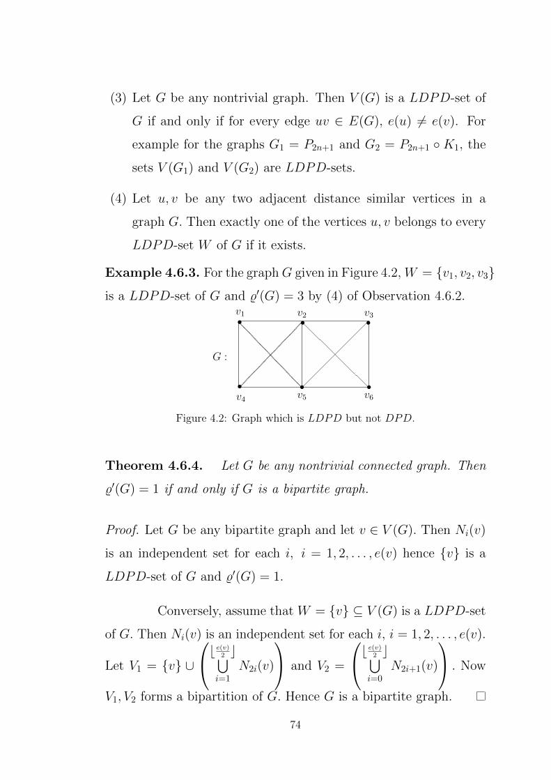
(3) Let G be any nontrivial graph. Then V (G) is a LDPD-set of

G if and only if for every edge uv ∈ E(G), e(u) 6= e(v). For

example for the graphs G1 = P2n+1 and G2 = P2n+1 K1, the

sets V (G1) and V (G2) are LDPD-sets.

(4) Let u, v be any two adjacent distance similar vertices in a

graph G. Then exactly one of the vertices u, v belongs to every

LDPD-set W of G if it exists.

Example 4.6.3. For the graphG given in Figure 4.2, W = v1, v2, v3

is a LDPD-set of G and %′(G) = 3 by (4) of Observation 4.6.2.

s

ss

s

s

sv1 v2 v3

v4 v5 v6

G :

Figure 4.2: Graph which is LDPD but not DPD.

Theorem 4.6.4. Let G be any nontrivial connected graph. Then

%′(G) = 1 if and only if G is a bipartite graph.

Proof. Let G be any bipartite graph and let v ∈ V (G). Then Ni(v)

is an independent set for each i, i = 1, 2, . . . , e(v) hence v is a

LDPD-set of G and %′(G) = 1.

Conversely, assume that W = v ⊆ V (G) is a LDPD-set

of G. Then Ni(v) is an independent set for each i, i = 1, 2, . . . , e(v).

Let V1 = v ∪

b e(v)2 c⋃i=1

N2i(v)

and V2 =

b e(v)2 c⋃i=0

N2i+1(v)

. Now

V1, V2 forms a bipartition of G. Hence G is a bipartite graph.

74

Corollary 4.6.5. For the n-dimensional hypercube Qn, n ≥ 3,

%′(Qn) = 1.

Theorem 4.6.6. Let G be any complete k-partite graph with

k ≥ 3. Then G is a LDPD-graph if and only if k = 3 and G

is not isomorphic to K3. Further if G is a LDPD-graph, then

%′(G) = min|Vi| : |Vi| ≥ 2+ 1.

Proof. Let V1 ∪ V2 ∪ · · · ∪ Vk be the k-partition of V (G) and let

W′

be any LDPD-set of G. If |Vi ∩W′| ≥ 2 and |Vj ∩W

′| ≥ 2 or

|Vi ∩W′| = |Vj ∩W

′| = 1 for some i 6= j, then fW ′(u) = fW ′(v) =

0, 1, 2 or fW ′(u) = fW ′(v) = 0, 1 respectively where u ∈ Vi∩W′

and v ∈ Vj ∩W′, a contradiction. Also if |Vi ∩W

′| = |Vj ∩W′| = 0

for some i 6= j, then fW ′(u) = fW ′(v) = 0, 1, where u ∈ Vi

and v ∈ Vj, which is again a contradiction. Hence we assume that

|V1 ∩W′| ≥ 2, |V2 ∩W

′| = 1 and |Vt ∩W′| = 0 for all t, 3 ≤ t ≤ k.

Suppose k ≥ 4. Then fW ′(x) = fW ′(y) = 1, 2 for all x ∈ V3

and y ∈ V4. Hence k = 3. Assume G is not isomorphic to K3. Let

V (G) = V1 ∪ V2 ∪ V3 be the tri-partition of V (G) with |V1| ≥ 2. Let

W = V1 ∪ y, where y ∈ V2. Then

fW (x) =

0, 1, 2 if x ∈ V1

1, 2 if x ∈ V2 − y

1 if x ∈ V3

and fW (y) = 0, 1. Hence W is a LDPD-set of G. Further, %′(G) =

min|Vi| : |Vi| ≥ 2+ 1.

Conversely, if G isomorphic to K3, clearly G has no

LDPD-set.

75

Theorem 4.6.7. Let G be any unicyclic graph. Then G is a LDPD-

graph if and only if G is not isomorphic to C3 or C5. Further if G

is a LDPD-graph, then

%′(G) =

1 if G is bipartite

2 if G ∼= C2k+1

3 otherwise.

Proof. Let G be any unicyclic graph and G 6= C3 or C5. Let C be the

unique cycle in G. If the length of C is even, then G is a bipartite

graph. Hence %′(G) = 1 by Theorem 4.6.4.

Suppose G = C2k+1 : (v1, v2, . . . , v2k+1, v1) for some k ≥ 3.

Then by Theorem 4.3.1 G admits a LDPD-set of order three and

by Theorem 4.6.4 we have %′(G) ≥ 2. Now we prove that there

is no LDPD-set of cardinality two in G. Let W1 = vi, vj be

any subset of V (G). Let P1 and P2 be the distinct paths join-

ing vi and vj. Then exactly one of l(P1) or l(P2) is odd. Sup-

pose l(P1) is odd and cen(P1) = x, y, where xy ∈ E(G). Then

fW1(x) = fW1

(y) = r(P1), r(P1)+1. Hence W1 is not a LDPD-set.

Therefore %′(G) = 3.

Now we assume that G properly contains C2k+1 for some

k ≥ 1. Let C2k+1 = (v1, v2, . . . , v2k+1). Suppose there exists

x ∈ V (G) − V (C2k+1) which is adjacent to v2. Let W2 = v1, x.

Now, fW2(vi) = i − 1 if 2 ≤ i ≤ k + 1, fW2

(vi) = 2(k + 1) −

i, 2(k + 2) − i if k + 3 ≤ i ≤ 2k + 1, fW2(vk+2) = k, k + 1 and

76

if uv ∈ E(G) − E(C2k+1), then fW2(u) = fW2

(v) + 1 or fW2(v) =

fW2(u) + 1. Hence W2 is a LDPD-set of G and %′(G) = 2.

Conversely, if G is isomorphic to C3 or C5, then G has no

LDPD-set.

Proposition 4.6.8. Let G be the sequential join of k copies of K2.

Then G is a LDPD graph if and only if k is odd. Further if G is a

LDPD-graph, then %′(G) = k.

Proof. Let V (G) =k⋃

i=1

Vi(K2), where Vi(K2) = ui, vi, 1 ≤ i ≤ k.

Let W be any LDPD-set of G if it exists. Then |Vi(K2) ∩W | = 1

for all i = 1, 2, . . . , k by (4) of Observation 4.6.2. Hence with-

out loss of generality we assume that W = u1, u2, . . . , uk. Sup-

pose k is odd. Then fW (ui) = fW (uk+1−i) = 0, 1, 2, . . . , k − i

for all i = 1, 2, . . . ,⌊k2

⌋, fW (ubk2c+1) = 0, 1, 2, . . . ,

⌊k2

⌋, fW (vi) =

fW (vk+1−i) = 1, 2, . . . , k−i for all i = 1, 2, . . . ,⌊k2

⌋and fW (vbk2c+1)

= 1, 2, . . . ,⌊k2

⌋. Therefore W is a LDPD-set of G and %′(G) = k.

Conversely, if k is even, then fW (ubk2c) = fW (ubk2c+1) =

0, 1, 2, . . . ,⌊k2

⌋. Hence W is not a LDPD-set. Therefore G is not

a LDPD-graph.

The following theorem shows that the graph obtained by

attaching any number of trees at any set of vertices of a LDPD-

graph is again a LDPD-graph.

Theorem 4.6.9. Let H be any LDPD-graph with %′(H) = k. Let

G be a graph with core(G) = H. Then %′(G) ≤ k.

77

Proof. Since core(G) = H, G can be decomposed into subgraphs

H,T1, T2, . . . , Tt where each Ti is tree with exactly one vertex of Ti

identified to ui ∈ V (H) for all i = 1, 2, . . . , t. Since %′(H) = k,

there exists a LDPD-set W ⊆ V (H) of cardinality k. Now we

prove that W is a LDPD-set of G also. Since W is a LDPD-

set of H and dG(x, y) = dH(x, y) for all x, y ∈ V (H), we have

fW (u) 6= fW (v) for all uv ∈ E(H). Let uv ∈ E(G)−E(H). Without

loss of generality assume that uv ∈ E(Ti) for some i, 1 ≤ i ≤ t and

d(v, ui) = d(u, ui) + 1. Then fW (u) = fW (v) + 1. Hence W is a

LDPD-set of G and %′(G) ≤ k.

Remark 4.6.10. The bound %′(G) ≤ k in Theorem 4.6.9 can be

sharp as well as strict.

(1) Let H1 be the sequential join K2 + K2 + K2. Let G1 be the

graph obtained from H1 by identifying the centre of K1,2 at

exactly one vertex of H1. Then %′(H1) = 3 by Proposition 4.6.8

and it can be verified that %′(G1) = 3.

(2) Let H2 = C2k+1, k ≥ 3. Let G2 be any unicyclic graph which

contains H2 as a proper subgraph. Then %′(H2) = 3 and

%′(G2) = 2 by Theorem 4.6.7.

Theorem 4.6.11. Let G be any LDPD-graph. Then the trestled

graph Tk(G) of G is also a LDPD-graph. Further %′(Tk(G)) ≤

%′(G).

78

Proof. Let V (G) = v1, v2, . . . , vn and let e1i = v1

i v1t , e

2i = v2

i v2t , . . . ,

eki = vki vkt be the edges of Tk(G) corresponding to the edge ei =

vivt ∈ E(G), i = 1, 2, . . . ,m. Let W be any LDPD-set of G and let

x ∈ W. Since d(vji , x) = d(vi, x) + 1, we have fW (vji ) = fW (vi) + 1.

Also fW (vi) 6= fW (vj) for all vivj ∈ E(G). Hence fW (vji ) 6= fw(vjt )

for all j ∈ 1, 2, . . . , k and ei = vivt ∈ E(G). Hence W is a LDPD-

set of Tk(G). Therefore %′(Tk(G)) ≤ %′(G).

Theorem 4.6.12. Let G be any graph of order at least four. Then

G can be embedded into a LDPD-graph.

Proof. Let V (G) = v1, v2, . . . , vn. Let G′ be the graph obtained

fromG by identifying exactly one leaf of the path Pin+1 at vi, 1 ≤ i ≤

n. Let W = v′1, v′2, . . . , v′n ⊆ V (G′), where v′i is the pendent vertex

of Pin+1, 1 ≤ i ≤ n. We claim that W is a LDPD-set of G′. Since

in ∈ fW (vi) and in /∈ fW (vj) for i 6= j, we have fW (vi) 6= fW (vj)

for all vivj ∈ E(G). Now, let uv ∈ E(G′) − E(G). Without loss

of generality we assume that uv is an edge of Pin+1 for some i,

1 ≤ i ≤ n and d(v, vi) = d(u, vi) + 1. Then fW (v) = fW (u) −

d(u, vi) + 1 ∪ d(v, vi) hence fW (u) 6= fW (v). Therefore W is

a LDPD-set of G′.

Theorem 4.6.13. Given any positive integer k there exists a graph

G such that %′(G) = lmd(G) = k.

Proof. When k = 1, let G = K2. Then %′(G) = lmd(G) = 1.

When k ≥ 2, let G = K1 + kK2, where V (K1) = x and

Vi(K2) = ui, vi for i = 1, 2, . . . , k. Since ui and vi are adjacent

79

distance similar vertices in G, exactly one of ui or vi say ui for each

i = 1, 2, . . . , k belongs to every LDPD-set and local metric set of G.

Let W = u1, u2, . . . , uk. Then fW (ui) = 0, 2, fW (vi) = 1, 2 for

all i = 1, 2, . . . , k, fW (x) = 1 and u1, u2, . . . , uk, v1, v2, . . . , vk

are independent sets. Hence W is a LDPD-set. Therefore %′(G) =

lmd(G) = k.


G such that %′(G)− lmd(G) = k.

Proof. Let Fi be the graph obtained from the cycle C3 = (ai, bi, ci, ai)

and the path P3 = (xi, yi, zi) by identifying xi with ai. Let F ′i

be the graph obtained from two copies of cycles (vi, ui, wi, vi) and

(di, ei, fi, di) by identifying di with ui. Let Hi be the graph ob-

tained from the graphs Fi and F ′i by identifying ai of Fi with vi

of F ′i . Now let G be the graph obtained from the path P2k−1 :

(w′1, w′2, . . . , w

′2k−1) and Hi : i = 1, 3, 5, . . . , 2k − 1 by identi-

fying a vertex wi of Hi with the vertex w′i of P2k−1 for all i =

1, 3, 5, . . . , 2k − 1.

Now in G, both bi, ci and ei, fi are adjacent distance

similar vertices. Hence exactly one of bi or ci and exactly one of

ei or fi, say bi and ei, belong to every LDPD-set and local metric

set of G, i = 1, 3, 5, . . . , 2k − 1. Now, let W1 be any LDPD-set

G. If |V (Hi) ∩W1| = 2 for some i, i ∈ 1, 3, 5, . . . , 2k − 1, then

W1∩V (Hi) = bi, ei and fW1(vi) = fW1

(ui), a contradiction. Hence

|V (Hi)∩W1| ≥ 3 for all i = 1, 3, 5, . . . , (2k− 1). Hence |W1| ≥ k, so

that %′(G) ≥ 3k.

80

Now, let W = bi, ei, zi : i = 1, 3, 5, . . . , 2k − 1 and let

xy ∈ E(G). If x, y ∈ vi, ci, vi, yi, vi, wi, ui, fi, ui, wi,

then max fW (x) 6= max fW (y). If x = vi and y = ui, then 3 =

d(ui, zi) ∈ fW1(y) but 3 /∈ fW1

(x) hence fW (x) 6= fW (y). Let x = w′i,

y = w′i+1. Without loss of generality we assume that i is odd. Then

2 ∈ fW (w′i) but 2 /∈ fW (w′i+1) and W is an independent set. Hence

W is a LDPD-set of G. Therefore %′(G) ≤ 3k. Hence %′(G) = 3k.

Let W2 = bi, ei : i = 1, 3, 5, . . . , (2k−1). Since d(ci, ei) =

d(vi, ei) + 1, d(fi, bi) = d(ui, bi) + 1, we have code(vi) 6= code(ci)

and code(ui) 6= code(fi). Also d(yi, bi) = d(vi, bi) + 1, d(zi, bi) =

d(yi, bi) + 1. Hence code(zi) 6= code(yi) and code(yi) 6= code(vi).

Now d(wi, bi) = d(ui, bi) = d(vi, bi) + 1 and d(wi, ei) = d(ui, ei) + 1.

Hence code(wi), code(ai) and code(di) are mutually distinct. When

w′iw′i+1 ∈ E(G) and i is odd, d(w′i+1, bi) = d(w′i, bi) + 1 hence

code(w′i) 6= code(w′i+1) and W2 is an independent set. Hence W2

is a local metric set and lmd(G) = 2k. Thus %′(G) − lmd(G) =

3k − 2k = k.


G such that %′(G) = %(G) = k.

Proof. Assume k ≥ 3. Let G be the graph obtained from the path

P(k2)+1 = (v1, v2, . . . , v(k

2)+1) and Hi = C3 : (xi, ui, wi, xi) :

i = 1, 2, 4 . . . ,(i2

)+ 1, . . . ,

(k2

)+ 1 by identifying a vertex xi of

Hi with vi for all i = 1, 2, 4, . . . ,(i2

)+ 1, . . . ,

(k2

)+ 1 respectively.

Since ui and wi are adjacent distance similar vertices by (4) of

81

Observation 4.6.2 exactly one of ui or wi say ui, i = 1, 2, 4, . . . ,(i2

)+

1, . . . ,(k2

)+ 1 belongs to every DPD and LDPD sets of G. Let

W = u1, u2, u4, . . . , u(k2)+1. We claim that W is a DPD-set of G.

Let x = vi, y = vj or x = wi, y = wj or x = ui, y = uj

with i < j. If d(x, cen(G)) 6= d(y, cen(G)), then max fW (x) 6=

max fW (y). If d(x, cen(G)) = d(y, cen(G)), then d(y, u1), d(y, u2) ⊆

fW (y) but d(y, u1), d(y, u2) * fW (x). Hence fW (x) 6= fW (y).

Now, let x = vi, y = wj. If i = j, then max fW (x) < fW (y). If

i 6= j, then 1 ∈ fW (y) but 1 /∈ fW (x) when x 6= v1 and y 6= w2

and 1, 3 ⊆ fW (y) but 1, 3 * fW (x) in other case. Hence

fW (x) 6= fW (y). Thus W is a DPD-set and hence %(G) = k. Now

W1 = u1, u2, u4, . . . , u(k2)+1 is a DPD-set of G, W1 is a LDPD-set

of G and hence %′(G) = k.

4.7 LDPD-GRAPHS AND UNIVERSAL

VERTICES

In this section we prove that any LDPD-graph can have

at most two universal vertices and we characterize LDPD-graphs

having exactly two universal vertices and LDPD-graphs having ex-

actly one universal vertex.

Theorem 4.7.1. Let G be any LDPD-graph and let S be a pairwise

distance similar set of G. If 〈S〉 is isomorphic to a complete graph,

then |S| = 2 and |S ∩W | = 1 for every LDPD-set W of G.

82

Proof. Let W be any LDPD-set of G. If x, y ∈ W ∩S or x, y ∈ W −

S, then fW (x) = fW (y) since d(x, v) = d(y, v) for all v ∈ V −x, y.

Hence |S| = 2 and |S ∩W | = 1.

Theorem 4.7.2. Let G be any graph with at least three universal

vertices. Then G is not a LDPD-graph.

Proof. Let S be the set of all universal vertices of G and let W ⊂ V.

If |W∩S| ≥ 2, then any two vertices in W∩S have the same distance

pattern with respect to W. If |W ∩ S| ≤ 1, then any two vertices in

S−W have the same distance pattern with respect to W. Hence W

is not a LDPD-set of G. Therefore G is not a LDPD-graph.

Theorem 4.7.3. Let G be any graph of order at least five and having

exactly two universal vertices. Then G is a LDPD-graph if and only

if G is isomorphic to K2 + H, where H is a bipartite graph with

bipartition A,B such that every vertex of A has a non-neighbor in

B and |B| ≥ 2.

Proof. Let G be a LDPD-graph with exactly two universal ver-

tices u and v. Then G contains an odd cycle hence %′(G) ≥ 2 by

Theorem 4.6.4. Let W be any LDPD-set of G with |W | ≥ 2. Since

u and v are adjacent distance similar vertices, exactly one of u or

v, say u, belongs to W. Let V1 = V − u, v. Then fW (u) = 0, 1

and fW (v) = 1. Now let A = V1 − W and B = V1 ∩ W . If

B = w, then fW (u) = fW (w) = 0, 1, a contradiction. Hence

|B| ≥ 2. Also if a vertex of A is adjacent to all the vertices in B,

then fW (x) = fW (v) = 1 for all x ∈ A, a contradiction. Hence

83

fW (x) = 1, 2 for all x ∈ A and fW (y) = 0, 1, 2 for all y ∈ B.

Hence the vertices in A have the same distance pattern and the

vertices in B have the same distance pattern. Hence A and B are

independent sets. Further G is isomorphic to K2 + H, where H is

a bipartite graph with bipartition A,B such that every vertex of A

has a non-neighbor in B and |B| ≥ 2.

Conversely, suppose G = K2 + H where H is a bipartite

graph with bipartition A,B such that every vertex of A has a non-

neighbor in B and |B| ≥ 2. Let V (G) = V (K2) ∪ V (H), where

V (K2) = u, v. Now W = B ∪ u is a LDPD-set, since fW (u) =

0, 1, fW (v) = 1, fW (x) = 1, 2 for all x ∈ A and fW (y) =

0, 1, 2 for all y ∈ B. Hence G is a LDPD-graph.

Theorem 4.7.4. Let G be any graph with exactly one universal

vertex. Then G is a LDPD-graph if and only if G is isomorphic to

one of the following graphs:

(i). G = K1 + H1, where H1 is a tripartite graph with partite sets

A,B,C such that B ∪ C is independent set and each vertex of

A has a neighbor and a nonneighbor in B.

(ii). G = K1 + H2, where H2 is a 4-partite graph with partite sets

A,B,C and w where B ∪ C is an independent set, w is ad-

jacent to all the vertices of B and to no vertex of C, and each

vertex of A has a neighbor and a nonneighbor in B ∪ w.

84

(iii). G = K1 + H3, where H3 is a tripartite graph with partite sets

A,B,C where 〈B ∪ C〉 is isomorphic to K|B|,|C| and each vertex

of A has a nonneighbor in B and |B| ≥ 2.

(The sets A or C or both may be empty.)

Proof. Let G be a LDPD-graph with exactly one universal vertex

u and let W be any LDPD-set of G.

Case 1. W = u.

Then G = K1,n−1 by Theorem 4.6.4. Hence G is isomor-

phic to a graph given in (i) with A = C = ∅.

Case 2. u /∈ W.

Let |W | ≥ 2. Then fW (u) = 1 and fW (x) 6= 1 for

all x ∈ V − u. Let N(u) = V1 ∪ V2, where V1 = W and V2 =

N(u) −W . Since d(u) = n − 1, the eccentricity of w is at most 2

for all w ∈ W. Hence the possible distance patterns of vertices in W

are 0, 1, 0, 2 and 0, 1, 2 only.

Let x ∈ W be a vertex such that fW (x) = 0, 2. Sup-

pose there exists y ∈ W such that fW (y) = 0, 1, 2. Then there

exists z(6= x) ∈ W such that yz ∈ E(G) and d(z, x) = 2. Hence

fW (z) = 0, 1, 2, a contradiction. Therefore 0, 1, 2 is not a dis-

tance pattern of any vertex of W . Also 0, 1 is not a distance pat-

tern of any vertex of W − x, since otherwise 1 ∈ fW (x) = 0, 2,

a contradiction. Hence W is an independent set and 0, 2 is the

only distance pattern of vertices in W. Now the possible distance

85

pattern of vertices in V2 are 2 and 1, 2 only since d(G) = 2 and

fW (u) = 1. Let A = y ∈ V2 : fW (y) = 1, 2, B = W and

C = y ∈ V2 : fW (y) = 2. Then B ∪ C is an independent set,

and each vertex of A has a neighbor and a nonneighbor in B. Hence

in this case G is isomorphic to a graph given in (i).

Now, let x ∈ W be a vertex such that fW (x) = 0, 1, 2.

Since |W | ≥ 2, there exists w ∈ W with xw ∈ E(G) and fW (w) =

0, 1. Hence w is adjacent to all the vertices of W. Therefore 0, 2

is not a distance pattern of any vertex of W and the distance pattern

of vertices in W − w is 0, 1, 2 only. Hence 〈W 〉 ∼= K1,t, where

t = |W | − 1. Now the possible distance pattern of vertices in V2

are 1, 2 and 2 only. Let A = y ∈ V2 : fW (y) = 1, 2, B =

W −w and C = y ∈ V2 : fW (y) = 2. Then B∪C ∪w is an

independent set, each vertex of A has a neighbor and a nonneighbor

in B ∪w, and w is adjacent to all the vertices of B. Hence in this

case G is isomorphic to a graph given in (ii).

Case 3. u ∈ W and W 6= u.

In this case fW (u) = 0, 1 and fW (x) = 0, 1, 2 for all

x ∈ W − u. Hence W − u is an independent set in G. Since

u ∈ W, the possible distance patterns of vertices in V2 are 1 and

1, 2 only. Let A = y ∈ V (G) : fW (y) = 1, 2, B = W and

C = y ∈ V (G) : fW (y) = 1. Then 〈B ∪ C〉 is isomorphic to

K|B|,|C| and every vertex of A has a nonneighbor in B and |B| ≥ 2.

Hence in this case G is isomorphic to a graph given in (iii).

86

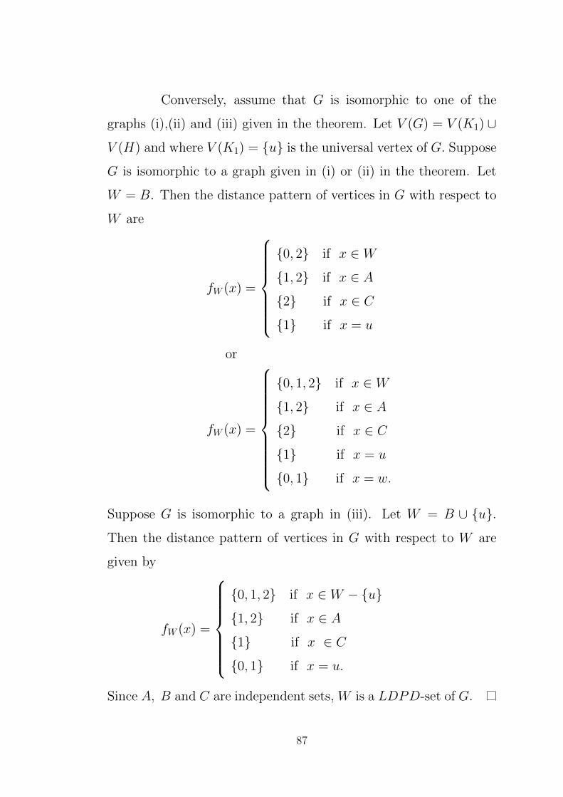
Conversely, assume that G is isomorphic to one of the

graphs (i),(ii) and (iii) given in the theorem. Let V (G) = V (K1) ∪

V (H) and where V (K1) = u is the universal vertex of G. Suppose

G is isomorphic to a graph given in (i) or (ii) in the theorem. Let

W = B. Then the distance pattern of vertices in G with respect to

W are

fW (x) =

0, 2 if x ∈ W

1, 2 if x ∈ A

2 if x ∈ C

1 if x = u

or

fW (x) =

0, 1, 2 if x ∈ W

1, 2 if x ∈ A

2 if x ∈ C

1 if x = u

0, 1 if x = w.

Suppose G is isomorphic to a graph in (iii). Let W = B ∪ u.

Then the distance pattern of vertices in G with respect to W are

given by

fW (x) =

0, 1, 2 if x ∈ W − u

1, 2 if x ∈ A

1 if x ∈ C

0, 1 if x = u.

Since A, B and C are independent sets, W is a LDPD-set of G.

87

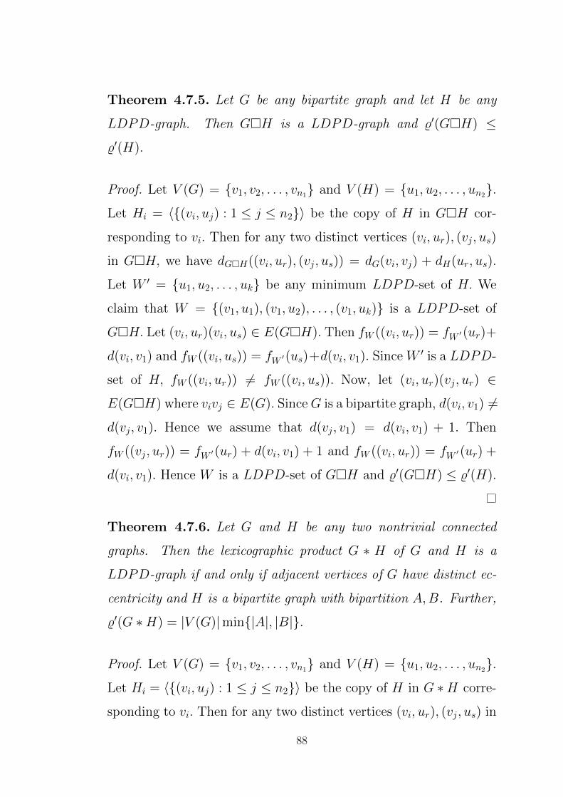
Theorem 4.7.5. Let G be any bipartite graph and let H be any

LDPD-graph. Then GH is a LDPD-graph and %′(GH) ≤

%′(H).


.

Let Hi = 〈(vi, uj) : 1 ≤ j ≤ n2〉 be the copy of H in GH cor-

responding to vi. Then for any two distinct vertices (vi, ur), (vj, us)

in GH, we have dGH((vi, ur), (vj, us)) = dG(vi, vj) + dH(ur, us).

Let W ′ = u1, u2, . . . , uk be any minimum LDPD-set of H. We

claim that W = (v1, u1), (v1, u2), . . . , (v1, uk) is a LDPD-set of

GH. Let (vi, ur)(vi, us) ∈ E(GH). Then fW ((vi, ur)) = fW ′(ur)+

d(vi, v1) and fW ((vi, us)) = fW ′(us)+d(vi, v1). Since W ′ is a LDPD-

set of H, fW ((vi, ur)) 6= fW ((vi, us)). Now, let (vi, ur)(vj, ur) ∈

E(GH) where vivj ∈ E(G). SinceG is a bipartite graph, d(vi, v1) 6=

d(vj, v1). Hence we assume that d(vj, v1) = d(vi, v1) + 1. Then

fW ((vj, ur)) = fW ′(ur) + d(vi, v1) + 1 and fW ((vi, ur)) = fW ′(ur) +

d(vi, v1). Hence W is a LDPD-set of GH and %′(GH) ≤ %′(H).


graphs. Then the lexicographic product G ∗ H of G and H is a

LDPD-graph if and only if adjacent vertices of G have distinct ec-

centricity and H is a bipartite graph with bipartition A,B. Further,

%′(G ∗H) = |V (G)|min|A|, |B|.


.

Let Hi = 〈(vi, uj) : 1 ≤ j ≤ n2〉 be the copy of H in G ∗H corre-

sponding to vi. Then for any two distinct vertices (vi, ur), (vj, us) in

88

G ∗H, we have

dG∗H((vi, ur), (vj, us)) =

dG(vi, vj) if i 6= j

1 if i = j and urus ∈ E(H)

2 otherwise.

Now, suppose G ∗H is a LDPD-graph. Let W be any LDPD-set

of G ∗ H. If V (Hi) ∩ W = ∅ or V (Hi) ∩ W = V (Hi) for some

i, 1 ≤ i ≤ n1, then fW ((vi, ur)) = fW ((vi, us)) for every edge

(vi, ur)(vi, us) ∈ E(Hi), since dG∗H((vi, ur), x) = dG∗H((vi, us), x) for

all x ∈ V (G∗H)−V (Hi), a contradiction. Hence 1 ≤ |V (Hi)∩W | ≤

|V (Hi)| − 1. Now, let (vi, ur) ∈ V (Hi) Then

fW ((vi, ur)) =

0, 1, 2, . . . , eG(vi) if (vi, ur) ∈ V (Hi) ∩W

1, 2, . . . , eG(vi) if (vi, ur) ∈ V (Hi)−W.Hence the sets V (Hi) ∩W and V (Hi)−W are independent sets in

Hi so that Hi is a bipartite graph. If there exists an edge vivj ∈

E(G) such that eG(vi) = eG(vj), then fW ((vi, ur)) = fW ((vj, us)) =

0, 1, 2 . . . , eG(vi) for all (vi, ur) ∈ V (Hi)∩W and for all (vj, us) ∈

V (Hj) ∩W , and fW ((vi, ur)) = fW ((vj, us)) = 1, 2 . . . , eG(vi) for

all (vi, ur) ∈ V (Hi)−W and for all (vj, us) ∈ V (Hj)−W, a contra-

diction. Hence no two adjacent vertices of G have same eccentricity.

Conversely, suppose H is a bipartite graph with bipartition

A,B and no two adjacent vertices of G have same eccentricity. Let

W ′ = (vi, ur) : 1 ≤ i ≤ n1, ur ∈ A. Now we claim that W ′

is a LDPD-set of G ∗ H. Let (vi, ur)(vj, us) ∈ E(G ∗ H). Then

vivj ∈ E(G) or i = j and urus ∈ E(H). If vivj ∈ E(G), then

max fW ′((vi, ur)) 6= max fW ′((vj, us)) since eG(vi) 6= eG(vj). Suppose

89

i = j and urus ∈ E(H). Then without loss of generality assume that

ur ∈ A and us ∈ B. Hence 0 ∈ fW ′((vi, ur)) but 0 /∈ fW ′((vi, us)).

Therefore W ′ is a LDPD-set of G ∗H.

We now claim that %′(G ∗H) = n1 min|A|, |B|. Without

loss of generality assume that |A| ≤ |B|. Let W be any LDPD-set of

G∗H. Then clearly 1 ≤ |V (Hi)∩W | ≤ n2−1 for all i = 1, 2, . . . , n1.

Suppose |W | < n1|A|. Then there exists i, 1 ≤ i ≤ n1 such that 1 ≤

|V (Hi) ∩W | < |A|. If there exists an edge (vi, ur)(vi, us) ∈ E(Hi)

such that (vi, ur) ∈ Ai−W and (vj, us) ∈ Bi−W, or (vi, ur) ∈ Ai∩W

and (vj, us) ∈ Bi ∩W, then fW ((vi, ur)) = fW ((vj, us)). Otherwise,

the graphs 〈(W ∩ Ai) ∪ (W ∩Bi)〉 and 〈(Ai −W ) ∪ (Bi −W )〉 are

totally disconnected and there is no path joining x and y where

x ∈ Ai − W and y ∈ Bi − W, which is not possible. Therefore

|V (Hi) ∩ Ai| ≥ |A| and hence %′(G ∗H) = n1 min|A|, |B|.

Conjecture 4.7.7. Let G be any connected graph in which no two

cycles have a common vertex or a common edge. Then G is a

LDPD-graph.

Conjecture 4.7.8. Let G be any LDPD-graph of order n. Then

%′(G) ≤⌈n2

⌉.


In this chapter we have initiated a study of dis-

tance pattern distinguishing sets, local distance pattern distinguish-

ing sets, distance pattern distinguishing number and local distance

90

pattern distinguishing number of a graph. The following are some

interesting problems for further investigation.

Problem 4.8.1. If G is a connected DPD-graph with diameter

d, does there exist a DPD-set M with |M | ≤ d?

Problem 4.8.2. Characterize trees which are DPD-graphs.

Problem 4.8.3. Given a positive integer k ≥ 3, does there exist

a k-regular DPD-graph?

Problem 4.8.4. Characterize graphs G for which %(G) = dim(G).

91

CHAPTER 5

NONDEFICIENT SETS IN GRAPHS

5.1 INTRODUCTION

Maximum matchings in bipartite graphs have interesting

applications. Let G = (V, E) be a bipartite graph with bipartition

V1 and V2, with |V1| ≤ |V2|. The following theorem of Hall [15] gives

a necessary and sufficient condition for the existence of a matching

M in G such that every vertex of V1 is matched to a vertex of V2

under M. There exists a matching M in G such that V1 is matched

to a subset of V2 under M if and only if |N(S)| ≥ |S| for all S ⊆ V1.

The condition |N(S)| ≥ |S| for all S ⊆ V is called Hall’s

condition. Motivated by this condition Chartrand and Lesniak [7]

defined a subset U of V to be nondeficient if |N(S)| ≥ |S| for every

nonempty subset S of U.

In this chapter, we initiate a study of nondeficient number

of graphs. We obtain sharp lower and upper bounds for nondeficient

number. Further we give a relation connecting nondeficient number

and the order of maximum critical independent set.

5.2 BASIC RESULTS

In this section, we introduce the concept of nondeficient

number nd(G) of a graph G and present several basic results.

Definition 5.2.1. The nondeficient number nd(G) of a graph G

is defined to be the maximum cardinality of a nondeficient set of

G. Any nondeficient set U of G with |U | = nd(G) is called a nd-set

of G.

Example 5.2.2. For the bistar G = B(r, s), nd(G) = 4. Also

nd(G) = |V (G)| for any graph G with a perfect matching.

Definition 5.2.3. [3] A subgraph H of G is called an elementary

subgraph of G if every component of H is either a cycle or an edge.

Elementary subgraphs play an important role in the com-

putation of the characteristic polynomial of the adjacency matrix

of a graph.

The following theorem provides a necessary and sufficient

condition for a subset U of V (G) to be a nondeficient set of a

graph G.

Theorem 5.2.4. Let G = (V,E) be any connected graph and let

U ⊆ V (G). Then U is a nondeficient set of G if and only if there

exists an elementary subgraph H of G such that U ⊆ V (H).

Proof. Let U be any nondeficient set of G and let Ω denote the fam-

ily of all open neighborhoods N(u) where u ∈ U (The members in

93

Ω are not necessarily distinct subsets of V ). Since |N(S)| ≥ |S|

for all S ⊆ U, it follows that the union of any k subsets in Ω

contains at least k elements. Hence by Theorem 1.3.12, the fam-

ily Ω has an SDR which we denote by f(u) : u ∈ U, where

f(u) ∈ N(u). Clearly f(u) 6= u and u is adjacent to f(u). Let

U1 = u ∈ U : f(u) ∈ U. Then α : U1 → U1 defined by α(u) = f(u)

is a permutation of U1 with α(u) 6= u. Hence α can be expressed as

a product of disjoint cyclic permutations, say α = α1α2 · · ·αr. The

cyclic permutation αi represents an edge in G if it is a transposi-

tion and a cycle in G otherwise. Now, let H be the edge induced

subgraph of G induced by the edges and cycles determined by the

αi’s and the set of edges u, f(u) : u ∈ U − U1. Clearly H is an

elementary subgraph of G and U ⊆ V (H).

Corollary 5.2.5. Let G be any connected graph and let U be a

nd-set of G. Then there exists an elementary subgraph H of G such

that V (H) = U.

Proof. Let U be any nd-set of G. By Theorem 5.2.4 there exists

an elementary subgraph H of G with U ⊆ V (H). Since V (H) is a

nondeficient set of G and U is a nd-set of G, we have U = V (H).

Corollary 5.2.6. For any graph G, nd(G) is the maximum order

of an elementary subgraph of G.

Corollary 5.2.7. Let G be any connected graph of order n. Then

nd(G) = n if and only if G has a spanning elementary subgraph.

94

Corollary 5.2.8. Let G be any connected bipartite graph of order

n. Then nd(G) = 2β1(G). In particular, nd(G) = n if and only if G

has a perfect matching.

Corollary 5.2.9. For almost all graphs G, we have nd(G) = n.

Proof. Since nd(G) = n if G is hamiltonian, the result follows from

the fact that almost all graphs are hamiltonian [22].

Now, we relate the parameter nd(G) to minimum cost flow

problem. Let x be an end vertex of an edge e; We denote the

incidence relation between x and e by x ∼ e or e ∼ x.

Definition 5.2.10. [26] Let f : E(G) → [0, 1] be a real valued

function. For any e ∈ E(G), f(e) is referred to as the weight of the

edge e. Define Ef = e ∈ E(G) : f(e) > 0 and let G 〈Ef〉 be the

subgraph of G induced by Ef . If∑e∼v

f(e) = 1 is satisfied for each

vertex v ∈ V (G), then G 〈Ef〉 , or Gf for short, is called a fractional

1-factor of G with indicator function f.

Theorem 5.2.11. A nontrivial graph G has a spanning elemen-

tary subgraph if and only if G has a fractional 1-factor.

Proof. Let H be any spanning elementary subgraph of G. Now, we

define a function f ′ : E(G)→ [0, 1] as follows:

f ′(e) =

1 if e is an edge component of H

12 if e is in a cycle component of H

0 if e /∈ E(H).

95

Then clearly G 〈Ef ′〉 is a fractional 1-factor of G. Conversely, assume

that G has a fractional 1-factor G 〈Ef〉 . Then by integrality theorem

for network flows, there exists a fractional 1-factor G 〈Eg〉 such that

for each edge e of G, g(e) is 0 or 12 or 1. Let H = H1 ∪ H2, where

H1 = 〈e ∈ E(G) : g(e) = 1〉 and H2 =⟨e ∈ E(G) : g(e) = 1

2⟩.

Then H is a spanning elementary subgraph of G where H1 is a union

of edges and H2 is a union of cycles.

Remark 5.2.12. An SDR for a finite family of finite sets, if it

exists, can be determined by the maxflow mincut algorithm ([12],

Page 68). Hence the elementary subgraph H of G in Theorem 5.2.4

and nd(G) can be determined by a polynomial time algorithm.

In the following proposition we characterize graphs G for

which nd(G) ∈ 2, 3, 4, 5.

Theorem 5.2.13. Let G be any nontrivial graph. Then

(i) nd(G) = 2 if and only if G is a star.

(ii) nd(G) = 3 if and only if G = K3.

(iii) nd(G) = 4 if and only if β1(G) = 2 and G has no subgraph

isomorphic to K2 ∪K3 or C5.

(iv) nd(G) = 5 if and only if β1(G) = 2 and G has a subgraph

isomorphic to K2 ∪K3 or C5.

96

Proof. Let S be any nd-set of G.

(i) Let nd(G) = 2. It follows from Theorem 5.2.4 that G

contains no cycle and β1(G) = 1. Hence G is a bipartite graph with

β1(G) = 1. Therefore G is a star.


(ii) Let nd(G) = 3. It follows from Theorem 5.2.4 that girth

of G is at most 3 and β1(G) = 1. Hence 〈S〉 = K3. If V − S 6= ∅,

then at least one vertex of S is adjacent to some vertex of V − S

and hence β1(G) ≥ 2, a contradiction. Hence G = K3.


(iii) Let nd(G) = 4. Then it follows from Theorem 5.2.4

that 〈S〉 contains 2K2 or C4. Also g(G) ≤ 4 and β1(G) ≤ 2. Hence

G has no subgraph isomorphic to K2 ∪K3 or C5.


(iv) Let nd(G) = 5. It follows from Theorem 5.2.4 that

g(G) ≤ 5 and β1(G) ≤ 2. Also if β1(G) = 1, then G is a star or K3

and hence nd(G) ≤ 4, which is a contradiction. Hence β1(G) = 2.

Now, 〈S〉 = K2 ∪K3 or C5 and thus G contains K2 ∪K3 or C5.


Remark 5.2.14. Let H be an elementary subgraph of G of order

nd(G) and having maximum number of components and let S =

V (G)− V (H). Then the following are true.

97

(i) Every component of H is either an edge or an odd cycle.

(ii) The set S is either empty or an independent set.

(iii) If v ∈ S, then v is not adjacent to any vertex of any odd cycle

in H.

(iv) If e = xy is a component of H and v ∈ S is adjacent to x, then

y is not adjacent to any vertex in S and y is not adjacent to

any vertex of any odd cycle in H.

(v) If u1 and u2 are two vertices in two distinct odd cycles in H,

then u1u2 /∈ E(G).

(vi) If e1 = x1y1 and e2 = x2y2 are components in H, u, v ∈ S and

ux1, vx2 ∈ E(G), then y1y2 /∈ E(G).

(vii) If an odd cycle Cr, r ≥ 5 is a component of H, then Cr is an

induced cycle in G.

Lemma 5.2.15. Let e = uv be a pendant edge of G with deg(v) =

1. Then there exists a maximum order elementary subgraph H of G,

which contains e as a component.

Proof. Let H be a maximum order elementary subgraph of G hav-

ing maximum number of components. Suppose e = uv is not a

component of H. Clearly u ∈ V (H) and it follows from (iii) of

Remark 5.2.14 that the component H1 of H which contains u is an

edge. Now K = (H − H1) ∪ e, is an elementary subgraph of G

and |V (K)| = |V (H)|.

98

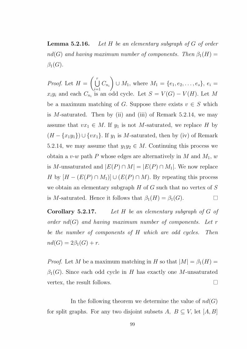
Lemma 5.2.16. Let H be an elementary subgraph of G of order

nd(G) and having maximum number of components. Then β1(H) =

β1(G).

Proof. Let H =

(r⋃

i=1

Cni

)∪M1, where M1 = e1, e2, . . . , es, ei =

xiyi and each Cniis an odd cycle. Let S = V (G) − V (H). Let M

be a maximum matching of G. Suppose there exists v ∈ S which

is M -saturated. Then by (ii) and (iii) of Remark 5.2.14, we may

assume that vx1 ∈ M. If y1 is not M -saturated, we replace H by

(H −x1y1)∪ vx1. If y1 is M -saturated, then by (iv) of Remark

5.2.14, we may assume that y1y2 ∈ M. Continuing this process we

obtain a v-w path P whose edges are alternatively in M and M1, w

is M -unsaturated and |E(P ) ∩M | = |E(P ) ∩M1|. We now replace

H by [H − (E(P ) ∩M1)] ∪ (E(P ) ∩M). By repeating this process

we obtain an elementary subgraph H of G such that no vertex of S

is M -saturated. Hence it follows that β1(H) = β1(G).

Corollary 5.2.17. Let H be an elementary subgraph of G of

order nd(G) and having maximum number of components. Let r

be the number of components of H which are odd cycles. Then

nd(G) = 2β1(G) + r.

Proof. Let M be a maximum matching in H so that |M | = β1(H) =

β1(G). Since each odd cycle in H has exactly one M -unsaturated

vertex, the result follows.

In the following theorem we determine the value of nd(G)

for split graphs. For any two disjoint subsets A, B ⊆ V, let [A,B]

99

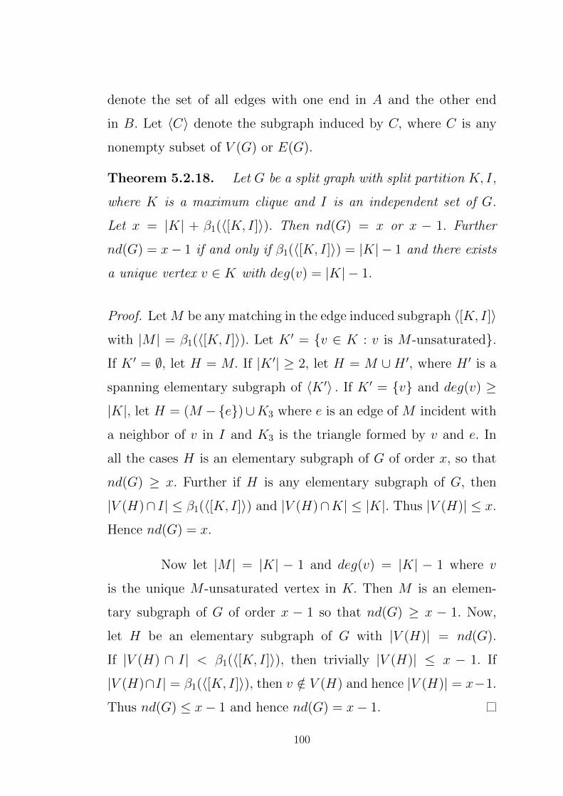
denote the set of all edges with one end in A and the other end

in B. Let 〈C〉 denote the subgraph induced by C, where C is any

nonempty subset of V (G) or E(G).

Theorem 5.2.18. Let G be a split graph with split partition K, I,

where K is a maximum clique and I is an independent set of G.

Let x = |K| + β1(〈[K, I]〉). Then nd(G) = x or x − 1. Further

nd(G) = x− 1 if and only if β1(〈[K, I]〉) = |K| − 1 and there exists

a unique vertex v ∈ K with deg(v) = |K| − 1.

Proof. Let M be any matching in the edge induced subgraph 〈[K, I]〉

with |M | = β1(〈[K, I]〉). Let K ′ = v ∈ K : v is M -unsaturated.

If K ′ = ∅, let H = M. If |K ′| ≥ 2, let H = M ∪H ′, where H ′ is a

spanning elementary subgraph of 〈K ′〉 . If K ′ = v and deg(v) ≥

|K|, let H = (M −e)∪K3 where e is an edge of M incident with

a neighbor of v in I and K3 is the triangle formed by v and e. In

all the cases H is an elementary subgraph of G of order x, so that

nd(G) ≥ x. Further if H is any elementary subgraph of G, then

|V (H)∩ I| ≤ β1(〈[K, I]〉) and |V (H)∩K| ≤ |K|. Thus |V (H)| ≤ x.

Hence nd(G) = x.

Now let |M | = |K| − 1 and deg(v) = |K| − 1 where v

is the unique M -unsaturated vertex in K. Then M is an elemen-

tary subgraph of G of order x − 1 so that nd(G) ≥ x − 1. Now,

let H be an elementary subgraph of G with |V (H)| = nd(G).

If |V (H) ∩ I| < β1(〈[K, I]〉), then trivially |V (H)| ≤ x − 1. If

|V (H)∩I| = β1(〈[K, I]〉), then v /∈ V (H) and hence |V (H)| = x−1.

Thus nd(G) ≤ x− 1 and hence nd(G) = x− 1.

100

5.3 BOUNDS

In this section we obtain sharp lower and upper bounds

for nd(G). Also we derive an elegant formula for nd(G).

Observation 5.3.1. It follows from Corollary 5.2.17 that for any

graph G of order at least three, 2β1(G) ≤ nd(G) ≤ 3β1(G) and

nd(G) = 3β1(G) if and only if G = kK3 where k = β1(G).

Theorem 5.3.2. Let G be any connected graph of order at least

four. Then nd(G) ≤ 3β1(G) − 1. Further, nd(G) = 3β1(G) − 1 if

and only if G is obtained from H = (β1(G) − 1)K3 ∪K1,t, t ≥ 1 by

joining the centre of K1,t to at least one vertex of each K3 in H.

Proof. Since G is connected, it follows from Observation 5.3.1 that

nd(G) ≤ 3β1(G) − 1. Now let G be any connected graph with

nd(G) = 3β1(G) − 1. Let H be an elementary subgraph of G of

order nd(G) = 3β1(G) − 1 with maximum number of components.

It follows from Corollary 5.2.17 that H = (β1(G)−1)K3∪K2. Since

V1 = V (G) − V (H) is an independent set and no vertex in V1 is

adjacent to any vertex of any odd cycle in H, it follows that each

vertex in V1 is adjacent to exactly one end vertex x of K2 in H.

Since there is no adjacency between any two K3’s in H and β1(H) =

β1(G), the vertex x is adjacent to at least one vertex of each K3 in

H.


101

Theorem 5.3.3. Given three positive integers a, b, c with 2a ≤

b ≤ c, a ≥ 2 and b ≤ 3a− 1, there exists a connected graph G with

β1(G) = a, nd(G) = b and |V (G)| = c.

Proof. If 2a = b ≤ c, let G be the graph obtained from the cycle

C2a−1 and the star K1,c−2a+1 by identifying the center of K1,c−2a+1

with a vertex of C2a−1. If 2a < b ≤ c, let G be the graph obtained

from H1 = (b−2a)K3∪ (3a− b−1)K2 and H2 = K1,c−b+1 by joining

the center of H2 to exactly one vertex of each component of H1.

Clearly β1(G) = a, |V (H)| = c and nd(G) = b.

Theorem 5.3.4. Let G be a connected graph of order n ≥ 2. Then

nd(G) ≥ n − β0(G) + 1, where β0(G) is the independence number

of G. Further equality holds if and only if G is either the complete

graph Kn or the star K1,n−1.

Proof. The inequality is obvious if nd(G) = n. Suppose nd(G) <

n. Let H be an elementary subgraph of G of order nd(G) having

maximum number of components. Let S = V (G)−V (H). It follows

from (ii), (iii) and (iv) of Remark 5.2.14 that there exists v ∈ V (H)

such that S ∪v is independent. Hence β0(G) ≥ n−nd(G) + 1, so

that nd(G) ≥ n−β0(G)+1. Now, suppose nd(G) = n−β0(G)+1. If

nd(G) = n, then β0(G) = 1 and hence G is the complete graph Kn.

Suppose nd(G) < n. Then there exists a unique vertex x ∈ V (H)

such that x is nonadjacent to every vertex in S. Hence by (iii) of

Remark 5.2.14, every component of H is K2. Now it follows from

(iv) of Remark 5.2.14 that H = K2 and hence G is isomorphic to

the star K1,n−1.

102

Now, we present a lower bound for nd(G) in terms of

rank(G).

Theorem 5.3.5. [5] Let f(G, λ) = λn + a1λn−1 + · · ·+ an be the

characteristic polynomial of the adjacency matrix A(G) of G. Then

ai =∑H

(−1)p(H)2c(H) where the sum is taken over all elementary

subgraphs H of G having exactly i vertices, p(H) denotes the total

number of components of H and c(H) denotes the number of cycles

in H.

Definition 5.3.6. [5] The rank and the nullity of a graph G, de-

noted by rank(G) and η(G) respectively, are defined to be the rank

and nullity of the adjacency matrix of G.

Theorem 5.3.7. Let G be any connected graph of order n. Then

nd(G) ≥ rank(G).

Proof. Let f(G, λ) = λn + a1λn−1 + · · · + an be the characteristic

polynomial of G and let nd(G) = k. Since G has no elementary

subgraph of order i, i > k, it follows from Theorem 5.3.5 that ai = 0

for all i > k. Hence η(G) ≥ n − k = n − nd(G). Thus nd(G) ≥

n− η(G) = rank(G).

Observation 5.3.8. The bound given in Theorem 5.3.7 is sharp.

For example we have nd(Kn) = rank(Kn) = n. Further the differ-

ence nd(G)− rank(G) can be made arbitrarily large. For the com-

plete bipartite graph Kr,r, we have nd(Kr,r) = 2r and

rank(Kr,r) = 2.

103

Now we derive an efficient formula for finding nondeficient

number of a graph G in terms of critical independence number of

G.

Definition 5.3.9. [1] An independent set of vertices Ic is a critical

independent set if |Ic| − |N(Ic)| ≥ |J | − |N(J)| for any independent

set J. A maximum critical independent set is a critical independent

set of maximum cardinality. The critical independence number of a

graph G, denoted as α′ = α′(G), is the cardinality of a maximum

critical independent set.

Definition 5.3.10. [21] A graph is independence irreducible if

α′ = 0. A graph is independence reducible if α′ > 0. A graph is

totally independence reducible if α′ = α, where α is an vertex inde-

pendence number of G.

Lemma 5.3.11. [20] If Ic is a critical independent set of G, then

there is a matching of the vertices N(Ic) into (a subset of) the

vertices of Ic.

Theorem 5.3.12. [21] For any graph G, there is a unique set

X ⊆ V (G) such that:

(i) α(G) = α(G 〈X〉) + α(G 〈Xc〉) where α(G) is the vertex inde-

pendent number of G,

(ii) G 〈X〉 is totally independence reducible,

(iii) G 〈Xc〉 is independence irreducible, and

(iv) for every maximum critical independent set Jc of G, X = Jc ∪

N(Jc).

104

Lemma 5.3.13. For any graph G, let Xc ⊆ V (G) be a subset of

V satisfying the condition of Theorem 5.3.12. Then for any subset

S ⊆ Xc, S has more than |S| neighbors in Xc.

Proof. Let S ′ = S−N(S). Then S ′ is an independent set in G 〈Xc〉

and N(S ′)∩ S = ∅. Further N(S ′) ⊆ Xc− S and, by Property (iii)

of Theorem 5.3.12, it follows that |N(S ′)| > |S ′|. Also S − S ′ ⊆

N(S−S ′). Thus N(S) ⊃ N(S ′)∪(S−S ′), which is a disjoint union.

Hence |N(S)| ≥ |N(S ′)|+ |N(S − S ′)| > |S ′|+ |S − S ′| = |S|.

Theorem 5.3.14. If Ic is a maximum critical independent set in

a graph G, then nd(G) = n− (|Ic| − |N(Ic)|).

Proof. Let Ic be a maximum critical independent set of G and

let X = Ic ∪ N(Ic). It follows from Lemma 5.3.11 that there is

a matching of vertices of N(Ic) into a subset of the vertices in

Ic. Let IM ⊆ Ic be the set of vertices matched to N(Ic). Then

|IM | = |N(Ic)|. Let U = IM∪N(Ic)∪Xc. Since these are disjoint sets,

|U | = |IM |+ |N(Ic)|+ |Xc| = (|Ic|− (|Ic|− |IM |)) + |N(Ic)|+ |Xc| =

(|Ic|+ |N(Ic)|+ |Xc|)− (|Ic| − |N(Ic)|) = n− (|Ic| − |N(Ic)|). So it

is enough to show that U is a maximum nondeficient set.

Let S ⊆ U. Then S = (IM ∩ S) ∪ (N(Ic) ∩ S) ∪ (Xc ∩ S),

and these sets are disjoint. Note that |N(IM ∩ S)| ≥ |IM ∩ S|,

as IM is matched to a set of vertices in N(Ic) disjoint from IM ;

|N(N(Ic)∩S)| ≥ |N(Ic)∩S|, for the same reason; and |N(Xc∩S)| ≥

|Xc ∩ S|, by Lemma 5.3.13. So |N(S)| ≥ |N(IM ∩ S)|+ |N(N(Ic)∩

S)| + |N(Xc ∩ S)| ≥ |IM ∩ S| + |N(Ic) ∩ S| + |Xc ∩ S| = |S|.

105

So U is nondeficient and nd(G) ≥ |U |.

Now let U ′ be any subset of V (G) with |U ′| > |U | = n −

(|Ic| − |N(Ic)|). Then |U ′ ∩ Ic| > |IM |. Hence |N(U ′)| < |U ′|. Thus

U ′ is not nondeficient. So nd(G) ≤ |U | = n− (|N(Ic)|− |Ic|). Hence

nd(G) = n− (|Ic| − |N(Ic)|).

Remark 5.3.15. [20] It is proved that maximum critical inde-

pendent set can be found efficiently and hence, N(Ic) can be found

efficiently. Therefore nd(G) can be computed in polynomial time

for any graph G.

Example 5.3.16. Consider the tree T given in Figure 5.1. Then

Ic = v1, v2, v3, v6, v7, v8 is the unique maximum critical indepen-

dent set of T and hence n− (|Ic| − |N(Ic)|) = 4. Also nd(T ) = 4 by

Corollary 5.2.8. ss

sss

ss s

v1

v2

v3

v4 v5

v6

v7

v8T

Figure 5.1: Tree with n− (|Ic| − |N(Ic)|) = 4 and nd(T ) = 4.

5.4 NONDEFICIENT SETS AND GRAPH OPERATIONS

In this section we determine the nondeficient number of

a graph which is obtained by applying graph operations on two

graphs.

106

Lemma 5.4.1. Let G be any connected graph of order n greater

than or equal to three. Then

nd(G+K1) =

nd(G) + 1 if nd(G) = n

nd(G) + 2 if nd(G) < n.

Proof. Let H be any maximum order elementary subgraph of G

having maximum number of components and let V (G + K1) =

V (G) ∪ v.

Suppose |V (H)| = n. If H contains an edge say e = ab

as a component, then (H − e) ∪ 〈a, b, v〉 is a spanning elemen-

tary subgraph of G + K1. If H contains an odd cycle say C2t+1 =

(v1, v2, . . . , v2t+1, v1) for some t ≥ 1 as a component, then (H −

C2t+1) ∪ v1v2, v3v4, . . . , v2t−1v2t, v2t+1v is a spanning elementary

subgraph of G+K1. Therefore nd(G+K1) = nd(G) + 1.

If |V (H)| < n, then H ∪〈uv〉 , where u ∈ V (G)−V (H), is

an elementary subgraph of G+K1. Hence nd(G+K1) ≥ nd(G) + 2.

Now, let H ′ be any maximum order elementary subgraph of G+K1.

Since |V (H ′)| ≥ nd(G) + 2, we have v ∈ V (H ′). Let H ′ = H1 ∪H2,

where H1 is the component of H containing v. If H1 = K2, then H2

is an elementary subgraph of G and hence nd(G+K1) ≤ nd(G)+2.

If H1 = C2t+1 for some t ≥ 1, then H2 ∪M, where M is a perfect

matching in the graph 〈V (C2t+1)− v〉 , is an elementary subgraph

of G of order at most nd(G). Hence nd(G+K1) ≤ nd(G) + 2. Thus

nd(G+K1) = nd(G) + 2.

107

Now we find the exact formula for nondeficient number of

corona of two graphs.

Theorem 5.4.2. Let G1 and G2 be two connected graphs of order

n1 and n2 respectively with n2 ≥ 3. Then

nd(G1 G2) =

|V (G1 G2)| if nd(G2) = n2

n1(nd(G2) + 2) if nd(G2) ≤ n2 − 1.

Proof. Let V (G1) = v1, v2, . . . , vn1. Since there exists a maximum

order elementary subgraph H of G1 G2 of the form H =n1⋃i=1

Hi,

where each Hi is a maximum order elementary subgraph of G+ vi,

it follows that nd(G1 G2) = n1nd(G2 + v). Hence the result follows

from Lemma 5.4.1.

In the following theorems we give lower bound for the non-

deficient number of the Cartesian product G1G2 and the Lexico-

graphic product G1 ∗G2 of two graphs G1 and G2.

Theorem 5.4.3. Let G1 and G2 be nontrivial connected graphs

of order n1 and n2 respectively. Then nd(G1G2) ≥ nd(G1)n2 +

(n1 − nd(G1))nd(G2) and the bound is sharp.

Proof. Let V (G1) = v1, v2, . . . , vn1 and V (G2) = u1, u2, . . . , un2

.

Let S1 = v1, v2, . . . , vk1 be a nd-set of G1. Then the induced

graph 〈S1 × V (G2)〉 of G1G2 contains a spanning elementary sub-

graph H ′. Now for each i, k1 < i ≤ n1, the induced graph Hi =

〈(vi, uj) : 1 ≤ j ≤ n2〉 contains an elementary subgraph H ′i of or-

der nd(G2). Hence the graph H ′ ∪

(n1⋃

i=k1+1

H ′i

)is an elementary

108

subgraph of G1G2 and hence nd(G1G2) ≥ nd(G1)n2 + (n1 −

nd(G1))nd(G2). Similarly

nd(G1G2) ≥ nd(G2)n1 + (n2 − nd(G2))nd(G1).

and hence the result follows.

Also for the graphs G1 = K3 and G2 = P3, nd(G1G2) =

nd(G1)n2 + (n1−nd(G1))nd(G2) and hence the bound is sharp.

Theorem 5.4.4. Let G1 and G2 be any two nontrivial connected

graphs of order n1 and n2 respectively. Then nd(G1∗G2) ≥ nd(G1)n2+

(n1 − nd(G1))nd(G2).

Proof. Similar to that of Theorem 5.4.3.

Remark 5.4.5. There exist graphs G1 and G2 with nd(G1 ∗

G2) > nd(G1G2). Let G1 = P3 and let G2 be the graph given in

Figure 5.2. s

sssss

Figure 5.2: Graph G2.

It can be easily verified that G1 ∗ G2 is hamiltonian and

hence nd(G1 ∗ G2) = 18. Further G1G2 is bipartite and does

not contain a perfect matching. Hence nd(G1G2) 6= 18. In fact

nd(G1G2) = 16.

109

In the following theorem we present the nondeficient num-

ber of trestled graph of any nontrivial graph.

Theorem 5.4.6. Let G be any nontrivial connected graph of order

n and size m. Then nd(Tk(G)) = 2mk + nd(G) where Tk(G) is the

trestled graph of G of index k.

Proof. Let V (G) = v1, v2, . . . , vn and E(G) = e1, e2, . . . , em.

Let e1i = v1

sv1t , e

2i = v2

sv2t , . . . , e

ki = vksv

kt be the edges of Tk(G)

corresponding to the edge ei = vsvt ∈ E(G), 1 ≤ i ≤ m. Let

H2 = eji : 1 ≤ i ≤ m, 1 ≤ j ≤ k. Let H1 be an elementary

subgraph of G with |V (H1)| = nd(G). Then H = H1 ∪H2 is an ele-

mentary subgraph of Tk(G) and hence nd(Tk(G)) ≥ 2mk + nd(G).

Now, let H ′ be any maximum order elementary subgraph of Tk(G)

having maximum number of components. Let ei ∈ E(G). Suppose

e1i /∈ E(H ′). Then at least one of the edges vsv

1s , vtv

1t is a component

of H ′, since otherwise H ′∪e1i is an elementary subgraph of Tk(G),

which is a contradiction. If both vsv1s , vtv

1t are components of H ′,

then we replace H ′ by (H ′−vsv1s , vtv

1t )∪ei, e1

i. If vsv1s ∈ E(H ′)

and vtv1t /∈ E(H ′), then we replace H ′ by (H ′−vsv1

s)∪e1i. Thus

we may assume without loss of generality that eji ∈ E(H ′), where

1 ≤ i ≤ m and 1 ≤ j ≤ k. Further there is no induced odd cycle in

Tk(G) containing the edge eji and hence it follows from (vii) of Re-

mark 5.2.14 that eji is a component of H ′. Thus H ′ = H2∪H3 where

H3 is an elementary subgraph of G. Hence nd(Tk(G)) ≤ |V (H ′)| ≤

2mk + nd(G). Therefore nd(Tk(G)) = 2mk + nd(G).

110

Theorem 5.4.7. Let G be any graph with nd(G) = |V (G)|. Then

nd(µ(G)) = |V (µ(G))|, where µ(G) is the Myceilskian graph of G.

Further if nd(G) < |V (G)|, then nd(µ(G)) ≥ 2nd(G) + 2 and the

bound is sharp.

Proof. Let V (G) = v1, v2, . . . , vn.

Case 1. nd(G) < |V (G)|.

Let H be an elementary subgraph of G having maximum

number of components with |V (H)| = nd(G). If an edge vivj is a

component of H, then we replace vivj by the two edges viv′j, vjv

′i.

Also for any odd cycle C2t+1 : (v1, v2, . . . , v2t+1, v1) in H, replace

C2t+1 by the (2t+1) edges v1v′2, v2v

′3, . . . , v2tv

′2t+1, v2t+1v

′1. Then H∪

ux′, where x ∈ V (G)− V (H) is an elementary subgraph of order

2nd(G) + 2. Hence nd(µ(G)) ≥ 2nd(G) + 2.

Case 2. nd(G) = |V (G)|.

If the elementary subgraph H of G contains an edge e =

vivj as a component, then we replace vivj by the cycle C5 : (vi, v′j, u,

v′i, vj, vi) and replace all the other components of H as in Case 1.

If every component in H is an odd cycle, then we replace one compo-

nent say (v1, v2, . . . , v2t+1, v1) ofH by (v1, v′2, v3, v

′4, . . . , v

′2t, v2t+1, v1)∪

v2v′3, v4v

′5, . . . , v2tv

′2t+1, v

′1u, and replace all the other components

of H as in Case 1. Thus we get a spanning elementary subgraph of

µ(G). Hence nd(µ(G)) = |V (µ(G))|.

111

The bound nd(µ(G)) ≥ 2nd(G) + 2 is sharp. For the

star G = K1,n, n ≥ 2, we have nd(G) = 2 and nd(µ(G)) = 6 =

2nd(G) + 2.


Motivated by the classical Hall’s theorem and the concept

of nondeficient set, we have introduced the nondeficient number of

a graph. The following are some interesting problems for further

investigation.

Problem 5.5.1. Characterize graphs G for which nd(G) = rank(G).

Problem 5.5.2. Characterize graphs G for which nd(µ(G)) =

2nd(G) + 2.

112

References

[1] A. Ageev, On finding critical independent and vertex sets,

SIAM J. Discrete Math., 7 (1994), 293–295.

[2] Z. Beerliova, F. Eberhard, T. Erlebach, A. Hall, M. Hoffman,

M. Mihalak, and L.S. Ram, Network discovery and verifica-

tion, IEEE Journal on Selected Areas in Communications, 24

(2006), 2168–2181.

[3] N. Biggs, Algebraic graph theory (Second Edition), Cambridge

University Press, 1996.

[4] J. A. Bondy and U.S.R. Murty, Graph Theory, Springer,2008.

[5] B. Borovicanin and I. Gutman, Nullity of graphs, Zb. Rad.

(Beogr.), 13(21) (2011), 107–122.

[6] F. Buckley and F. Harary, Distance in graphs, Addison Wesley,

CA, 1990.

[7] G. Chartrand and L. Lesniak, Graphs and Digraphs, Chapman

and Hall, CRC, Fourth Edition, 2005.

[8] G. Chartrand and P. Zhang, The theory and applications of

resolvability in graphs: A Survey, Congr. Numer., 160 (2003),

47–68.

[9] G. Chartrand and P. Zhang, Chromatic Graph Theory, Chap-

man and Hall, CRC, First Edition, 2009.

[10] G. Chartrand, L. Eroh, M. Johnson and O. R. Oellermann,

Resolvability in graphs and the metric dimension of a graph,

Discrete Appl. Math., 105 (2000), 99–113.

[11] V. Chvatal, Mastermind, Combinatorica, 3 (1983), 325–329.

[12] L. R. Ford, Jr. and D.R. Fulkerson, Flows in Networks, Prince-

ton University Press, 1962.

[13] M. C. Golumbic, Algorithmic Graph Theory and Perfect

Graphs, Elsevier, Second Edition, 2004.

[14] J. L. Gross and Jay Yellen, Hand book of Graph Theory, CRC

Press, New jersey, 2004.

[15] P. Hall, On representatives of subsets, J. Lond. Math. Soc., 10

(1935), 26–30.

[16] F. Harary and R. A. Melter, On the metric dimension of a

graph, Ars Combin., 2 (1976), 191–195.

[17] T. W. Haynes, S. T. Hedetniemi and P. J. Slater, Fundamentals

of Domination in Graphs, Marcel Dekker, Inc., New York, NY,

1998.

114

[18] C. Hernando, M. Mora, I. M. Pelayo and C. Seara, Extremal

Graph Theory for Metric Dimension and Diameter, Electron.

J. Combin., 17 (2010), #R30.

[19] S. Khuller, B. Raghavachari and A. Rosenfield, Landmarks in

graphs, Discrete Appl. Math., 70 (1996), 217–229.

[20] C. E. Larson, A Note on Critical Independence Reductions,

Bull. Inst. Combin. Appl., 51 (2007), 34–46.

[21] C. E. Larson, The critical independence number and an inde-

pendence decomposition, European J. Combin., 32(2) (2011),

294–300.

[22] J. W. Moon, Almost all graphs have a spanning cycle, Canad.

Math. Bull., 15(1) (1972), 39–41.

[23] J. Mycielski, Sur le colouriage des graphes, Colloq. Math., 3

(1955), 161–162.

[24] F. Okamoto, B. Phinezy and Ping zhang, On Local Metric Di-

mension of a Graph, J. Combin. Math. Combin. Comput., 72

(2010), 243–259.

[25] V. Saenpholphat and P. Zhang, Connected Resolvability of

Graphs, Czechoslovak Math. J., 53(128) (2003), 827–840.

[26] E. R. Scheinerman and D. H. Ullam, Fractional Graph Theory,

Willey, New York, 1997.

115

[27] A. Sebo and E. Tannier, On metric generators of graphs, Math.

Oper. Res., 29 (2004), 383–393.

[28] H. Shapiro and S. Soderberg, A combinatory detection prob-

lem, Amer. Math. Monthly, 70 (1963), 1066–1070.

[29] P. J. Slater, Leaves of trees, Congr. Numer., 14 (1975), 549–

559.

[30] P. J. Slater, Domination and location in acyclic graphs, Net-

works, 17 (1987), 55–64.

116

LIST OF PUBLICATIONS

1. R. Anantha Kumar and K. A. Germina, Distance Pattern

distinguishing sets in graphs, Adv. Stud. Contemp. Math.

(Kyungshang), 21 (2011), 107–114.

2. R. Anantha Kumar and S. Arumugam, Pairwise Distance

Similar Sets in Graphs, J. Combin. Math. Combin. Comput.,

84 (2013), 21–28.

3. S. Arumugam and R. Anantha Kumar, Distance Similar Sets

in Graphs, Util. Math., (Accepted).

117

VITAE

Mr. R. ANANTHA KUMAR was born on

16th October 1983 at Srivilliputtur, Tamil Nadu, India. He received

his Bachelor’s degree in Mathematics in 2003, Master’s degree in

Mathematics in 2005 and Master of Philosophy in Mathematics in

2006, all from Madurai Kamaraj University, Madurai.

He started his research career at Kalasalingam University

as a Research Fellow of the Department of Science and Technology

Sponsored Research Project SR/S4/MS: 427/07.

He has attended several national and international

conferences and has presented papers. He is actively involved in

research for the past five years. Two of his research papers have

been published and one paper has been accepted for publication.

118

STUDIES IN GRAPH THEORY - DISTANCE RELATED CONCEPTS IN...

Documents

Transcript of STUDIES IN GRAPH THEORY - DISTANCE RELATED CONCEPTS IN...