Studie av subsynkron interaktion (SSTI) mellan ett HVDC ...518005/FULLTEXT01.pdf · torsional...

Studie av subsynkron interaktion (SSTI) mellan ett HVDC system med spänningsstyva strömriktare och en närliggande generator

Study of the Subsynchronous Torsional Interaction (SSTI) between the HVDC based on VSCs and the adjacent generator. Rolf Pålsson

EXAMENSARBETE Elektroteknik 2006 Nr: E3213E

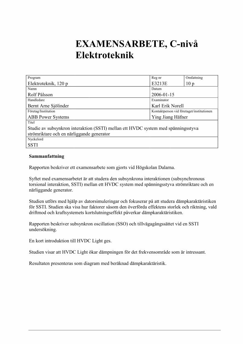
EXAMENSARBETE, C-nivå Elektroteknik

Program Reg nr Omfattning Elektroteknik, 120 p E3213E 10 p Namn Datum Rolf Pålsson 2006-01-15 Handledare Examinator Bernt Arne Sjölinder Karl Erik Norell Företag/Institution Kontaktperson vid företaget/institutionen ABB Power Systems Ying Jiang Häfner Titel Studie av subsynkron interaktion (SSTI) mellan ett HVDC system med spänningsstyva strömriktare och en närliggande generator Nyckelord SSTI Sammanfattning Rapporten beskriver ett examensarbete som gjorts vid Högskolan Dalarna. Syftet med examensarbetet är att studera den subsynkrona interaktionen (subsynchronous torsional interaktion, SSTI) mellan ett HVDC system med spänningsstyva strömriktare och en närliggande generator. Studien utförs med hjälp av datorsimuleringar och fokuserar på att studera dämpkaraktäristiken för SSTI. Studien ska visa hur faktorer såsom den överförda effektens storlek och riktning, vald driftmod och kraftsystemets kortslutningseffekt påverkar dämpkaraktäristiken. Rapporten beskriver subsynkron oscillation (SSO) och tillvägagångssättet vid en SSTI undersökning. En kort introduktion till HVDC Light ges. Studien visar att HVDC Light ökar dämpningen för det frekvensområde som är intressant. Resultaten presenteras som diagram med beräknad dämpkaraktäristik.

DEGREE PROJECT Electro Engineering

Programme Reg number Extent Electro Engineering E3213E 15 ECTS Name of student Year-Month-Day Rolf Pålsson 2006-01-15 Supervisor Examiner Bernt-Arne Sjölinder Karl-Erik Norell Company/Department Supervisor at the Company/Department ABB Power System Ying Jiang Häfner Title Study of the Subsynchronous Torsional Interaction (SSTI) between the HVDC system based on VSCs and the adjacent generator. Keywords SSTI

Summary The report describes a degree project at Högskolan Dalarna.

The purpose of this exam work is to study the subsynchronous torsional interaction (SSTI) between the HVDC based on VSCs and the adjacent generator unit.

The study is performed through computer simulation with EMTDC and focuses on studying the SSTI damping characteristics. The study results reveal how factors such as selected control modes, the transmitted power level and direction and the short circuit ratio of the a.c. network affect the SSTI damping characteristics.

The report describes the Subsynchronous Oscillation (SSO) and the procedure to be followed in SSTI investigation.

A short introduction to HVDC Light is given.

The study shows that the HVDC Light increases the damping characteristic for the frequency range of interest.

The results from the study are presented as plots with the calculated damping characteristic.

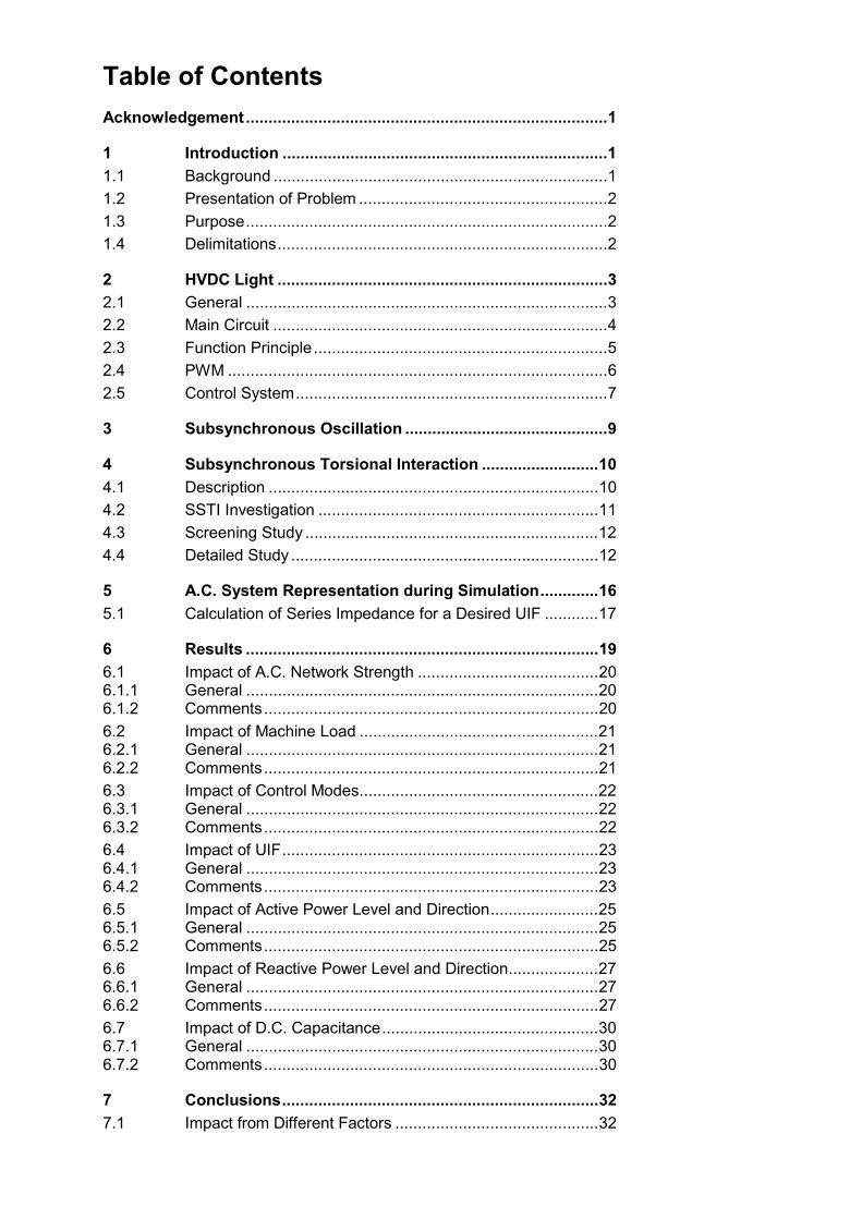
Table of Contents Acknowledgement................................................................................1

1 Introduction ........................................................................1 1.1 Background ..........................................................................1 1.2 Presentation of Problem .......................................................2 1.3 Purpose................................................................................2 1.4 Delimitations.........................................................................2

2 HVDC Light .........................................................................3 2.1 General ................................................................................3 2.2 Main Circuit ..........................................................................4 2.3 Function Principle.................................................................5 2.4 PWM ....................................................................................6 2.5 Control System.....................................................................7

3 Subsynchronous Oscillation .............................................9

4 Subsynchronous Torsional Interaction ..........................10 4.1 Description .........................................................................10 4.2 SSTI Investigation ..............................................................11 4.3 Screening Study .................................................................12 4.4 Detailed Study ....................................................................12

5 A.C. System Representation during Simulation.............16 5.1 Calculation of Series Impedance for a Desired UIF ............17

6 Results ..............................................................................19 6.1 Impact of A.C. Network Strength ........................................20 6.1.1 General ..............................................................................20 6.1.2 Comments..........................................................................20 6.2 Impact of Machine Load .....................................................21 6.2.1 General ..............................................................................21 6.2.2 Comments..........................................................................21 6.3 Impact of Control Modes.....................................................22 6.3.1 General ..............................................................................22 6.3.2 Comments..........................................................................22 6.4 Impact of UIF......................................................................23 6.4.1 General ..............................................................................23 6.4.2 Comments..........................................................................23 6.5 Impact of Active Power Level and Direction........................25 6.5.1 General ..............................................................................25 6.5.2 Comments..........................................................................25 6.6 Impact of Reactive Power Level and Direction....................27 6.6.1 General ..............................................................................27 6.6.2 Comments..........................................................................27 6.7 Impact of D.C. Capacitance................................................30 6.7.1 General ..............................................................................30 6.7.2 Comments..........................................................................30

7 Conclusions......................................................................32 7.1 Impact from Different Factors .............................................32

7.2 Comparison with Operation without HVDC Light ................33 7.3 General Conclusion ............................................................33

8 References. .......................................................................33

9 Appendix...........................................................................34 9.1 Appendix 1 .........................................................................34 9.2 Appendix 2 .........................................................................36

Degree Project, Högskolan Dalarna

- 1 -

Acknowledgement In the last month my knowledge about SSTI and the tools and programs for studies have increased a lot.

Thanks to:

Ying Jiang Häfner, supervisor for my work, for sharing her wide and deep knowledge.

Bernt Arne Sjölinder, supervisor at Högskolan Dalarna, for supervising and guiding me in shaping the work to scientific and academic standards.

Ingvar Hagman, for inspiring me to get started.

Thomas Tulkiewicz, for always having time for questions.

Per Holmberg, for useful comments when writing the report.

1 Introduction

1.1 Background In the 1970’s the first damage to a shaft on a generating unit caused by Subsynchronous Resonance (SSR) was reported [4]. The place was Mohave Generating Station in Southern Nevada. The resonance was established between mechanical modes on the turbine generator shaft and a series compensation on a transmission line.

Subsynchronous Torsional Interaction (SSTI) was observed for the first time in 1977 at Square Butte [4]. Under certain system conditions a torsional mode was destabilized by a current control loop from a High Voltage Direct Current (HVDC) converter.

Consequently interaction from series compensation and HVDC system with turbo generators in the area below the fundamental frequency is well known.

Much effort has been spent on research of the SSTI phenomena. Tools for examining and tools to assess expected interactions have been developed. The experience for HVDC built up with line commutated converters, in ABB called HVDC Classic, shows that SSTI can be avoided with a proper control design.

In 1997 ABB introduced a Voltage Source Converter (VSC) on the market, under the name HVDC Light. The knowledge about SSTI from HVDC Classic was not in all part applicable. Therefore, the need of new research was obvious.

Particularly, considering that HVDC Light is a relatively new product it is very important to make a systematical study about the SSTI damping characteristic in order to show to the market that the performance is acceptable.

Test of SSTI at the installed transmission links is one way to investigate the performance. However, as the numbers of installed stations close to turbo generators are few it is not possible to cover all conceivable applications. Field tests are also complicated and include a risk of unwanted incidents.

Computer simulations are simpler and more flexible when investigating the SSTI damping characteristic.


- 2 -

1.2 Presentation of Problem The aim when installing an HVDC Light system, with regards to SSTI, is that the SSTI damping characteristic should not be affected in a negative way. To be successful, the knowledge about what affects the damping characteristic must be increased.

To make a list of factors that probably affect the damping characteristic is not difficult, but the knowledge of how much the impact is from these factors, can probably only be reached by extensive computer simulations. In the simulation model it must be possible to change one factor without affecting another.

1.3 Purpose The purpose of this exam work is to study the SSTI between the HVDC based on VSCs and the adjacent generator unit [2].

The SSTI damping characteristics are probably affected by factors, such as:

• short circuit ratio (SCR) of the AC network

• machine load

• selected control modes of the VSC

• UIF

• transmitted active power level and direction

• reactive power level and direction

• capacitance at the d.c. side

The study results will reveal how these factors affect the SSTI damping characteristics.

1.4 Delimitations The study is delimited to one machine type and to a simple a.c. net configuration. The switching method is Optimised Pulse With Modulation (OPWM).


- 3 -

2 HVDC Light

2.1 General The HVDC technology is used to transmit electricity over long distances by overhead transmission lines or submarine cables. It is also used to interconnect separate power systems, where traditional a.c. connections can’t be used.

HVDC Light is a new power transmission technology developed by ABB. It is particularly suitable for medium to small-scale power transmission applications.

In high power applications, the converter is a line commutated Current Source Converter (CSC) built up with thyristors. This technology is called HVDC Classic. In HVDC Light, the converter is a self commutated Voltage Source Converter (VSC) built up with Insulated Gate Bipolar Transistors (IGBTs).

As an example Figure 1 shows a HVDC Light transmission system.

Figure 1. HVDC Light transmission system.


- 4 -

2.2 Main Circuit

Each station, shown in Figure 1, is comprised of transformer, harmonic filter, phase reactor and a converter bridge. Figure 2 shows a HVDC Light station.

Figure 2. Single line diagram for HVDC Light station.

Figure 3 shows the converter bridge. In this study it is a two level bridge. Two levels refer to the two potentials, +DC and –DC in the figure, that can be coupled to the a.c. phase terminals.

Figure 3. Two level converter bridge for HVDC Light applications.


- 5 -

2.3 Function Principle As an IGBT (e.g. VA.V1 in Figure 3) can be both turned on and off, it can be treated like a switch for easier understanding of the function principle. The IGBTs can couple the a.c. terminal to either the positive or the negative d.c. voltage. The simplest way to create an output voltage from the converter is to couple a.c. terminal to the positive d.c. voltage terminal during the positive half period and to the negative terminal during the negative half period, forming a square wave with fundamental frequency. The disadvantage with this method is that the only way to change the amplitude of the fundamental voltage is to change the d.c. voltage. The square wave also includes harmonics of low order.

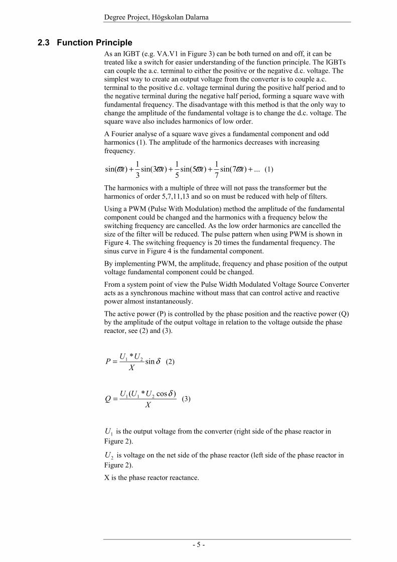
A Fourier analyse of a square wave gives a fundamental component and odd harmonics (1). The amplitude of the harmonics decreases with increasing frequency.

...)7sin(71)5sin(

51)3sin(

31)sin( ++++ tttt ϖϖϖϖ (1)

The harmonics with a multiple of three will not pass the transformer but the harmonics of order 5,7,11,13 and so on must be reduced with help of filters.

Using a PWM (Pulse With Modulation) method the amplitude of the fundamental component could be changed and the harmonics with a frequency below the switching frequency are cancelled. As the low order harmonics are cancelled the size of the filter will be reduced. The pulse pattern when using PWM is shown in Figure 4. The switching frequency is 20 times the fundamental frequency. The sinus curve in Figure 4 is the fundamental component.

By implementing PWM, the amplitude, frequency and phase position of the output voltage fundamental component could be changed.

From a system point of view the Pulse Width Modulated Voltage Source Converter acts as a synchronous machine without mass that can control active and reactive power almost instantaneously.

The active power (P) is controlled by the phase position and the reactive power (Q) by the amplitude of the output voltage in relation to the voltage outside the phase reactor, see (2) and (3).

δsin* 21

XUUP = (2)

XUUUQ )cos*( 211 δ= (3)

1U is the output voltage from the converter (right side of the phase reactor in Figure 2).

2U is voltage on the net side of the phase reactor (left side of the phase reactor in Figure 2).

X is the phase reactor reactance.


- 6 -

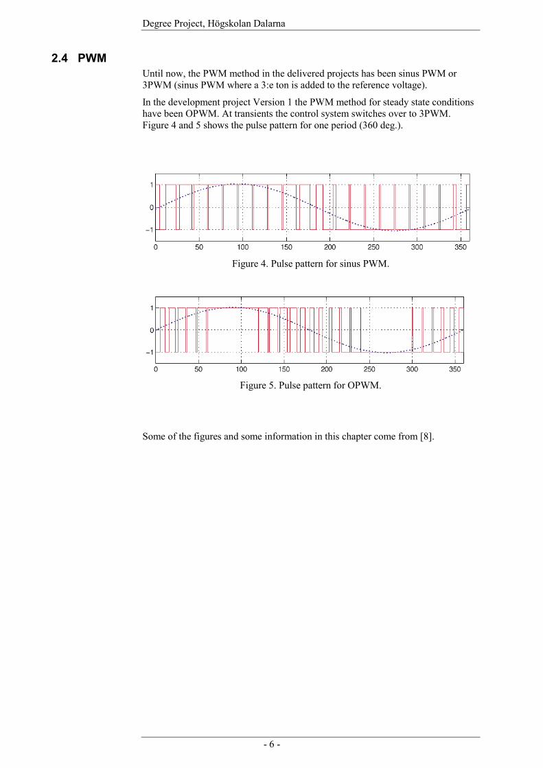
2.4 PWM Until now, the PWM method in the delivered projects has been sinus PWM or 3PWM (sinus PWM where a 3:e ton is added to the reference voltage).

In the development project Version 1 the PWM method for steady state conditions have been OPWM. At transients the control system switches over to 3PWM. Figure 4 and 5 shows the pulse pattern for one period (360 deg.).

Figure 4. Pulse pattern for sinus PWM.

Figure 5. Pulse pattern for OPWM.

Some of the figures and some information in this chapter come from [8].


- 7 -

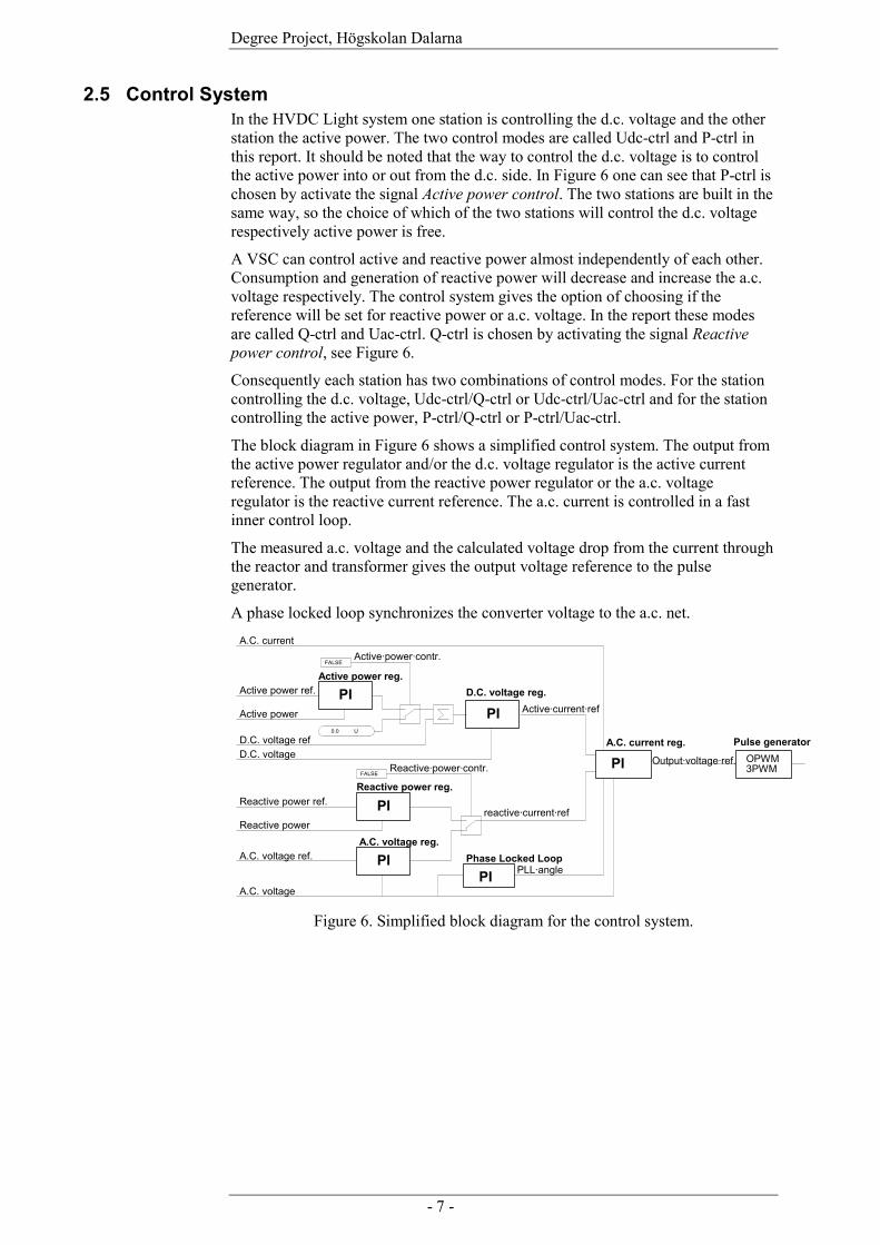
2.5 Control System In the HVDC Light system one station is controlling the d.c. voltage and the other station the active power. The two control modes are called Udc-ctrl and P-ctrl in this report. It should be noted that the way to control the d.c. voltage is to control the active power into or out from the d.c. side. In Figure 6 one can see that P-ctrl is chosen by activate the signal Active power control. The two stations are built in the same way, so the choice of which of the two stations will control the d.c. voltage respectively active power is free.

A VSC can control active and reactive power almost independently of each other. Consumption and generation of reactive power will decrease and increase the a.c. voltage respectively. The control system gives the option of choosing if the reference will be set for reactive power or a.c. voltage. In the report these modes are called Q-ctrl and Uac-ctrl. Q-ctrl is chosen by activating the signal Reactive power control, see Figure 6.

Consequently each station has two combinations of control modes. For the station controlling the d.c. voltage, Udc-ctrl/Q-ctrl or Udc-ctrl/Uac-ctrl and for the station controlling the active power, P-ctrl/Q-ctrl or P-ctrl/Uac-ctrl.

The block diagram in Figure 6 shows a simplified control system. The output from the active power regulator and/or the d.c. voltage regulator is the active current reference. The output from the reactive power regulator or the a.c. voltage regulator is the reactive current reference. The a.c. current is controlled in a fast inner control loop.

The measured a.c. voltage and the calculated voltage drop from the current through the reactor and transformer gives the output voltage reference to the pulse generator.

A phase locked loop synchronizes the converter voltage to the a.c. net.

0.0 U

FALSE

FALSE

Active power reg.

Reactive power reg.

A.C. voltage reg.

A.C. current

Pulse generator

Active power ref.

Active power

Reactive power ref.

Reactive power

A.C. voltage ref.

D.C. voltageA.C. current reg.

A.C. voltage

Phase Locked Loop

PI

PIPI

PI OPWM3PWM

PID.C. voltage reg.

Active·power·contr.

Reactive·power·contr.

Active·current·ref

reactive·current·ref

Output·voltage·ref.

PLL·angle

PI

D.C. voltage ref

Figure 6. Simplified block diagram for the control system.


- 8 -

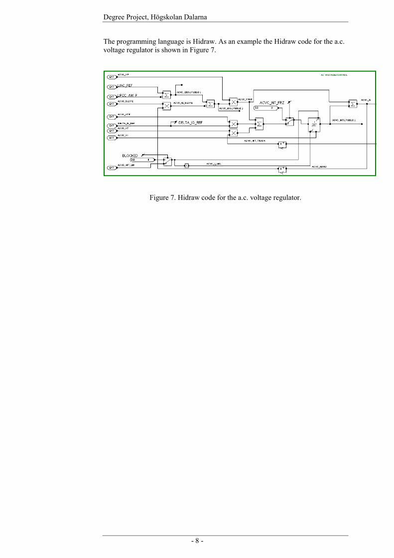
The programming language is Hidraw. As an example the Hidraw code for the a.c. voltage regulator is shown in Figure 7.

Figure 7. Hidraw code for the a.c. voltage regulator.


- 9 -

3 Subsynchronous Oscillation Subsynchronous oscillation (SSO) is interaction between a turbo generator and system elements in the a.c. network at frequencies below the system frequency.

When the resonance frequency in the network is caused by passive components, it’s called SSR.

When the oscillation is caused by an active system, e.g. HVDC converters, it’s called SSTI.

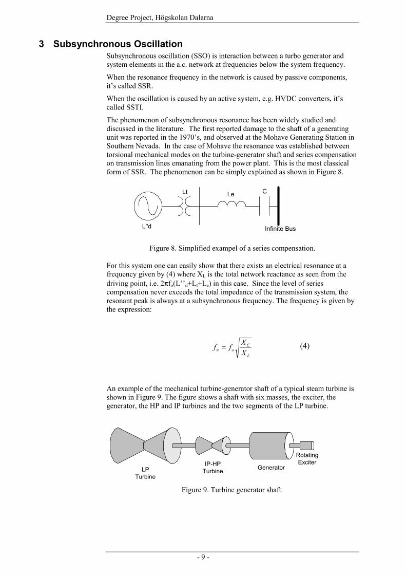
The phenomenon of subsynchronous resonance has been widely studied and discussed in the literature. The first reported damage to the shaft of a generating unit was reported in the 1970’s, and observed at the Mohave Generating Station in Southern Nevada. In the case of Mohave the resonance was established between torsional mechanical modes on the turbine-generator shaft and series compensation on transmission lines emanating from the power plant. This is the most classical form of SSR. The phenomenon can be simply explained as shown in Figure 8.

Infinite BusL''d

Lt Le C

Figure 8. Simplified exampel of a series compensation. For this system one can easily show that there exists an electrical resonance at a frequency given by (4) where XL is the total network reactance as seen from the driving point, i.e. 2πfo(L’’d+Lt+Le) in this case. Since the level of series compensation never exceeds the total impedance of the transmission system, the resonant peak is always at a subsynchronous frequency. The frequency is given by the expression:

L

Con X

Xff = (4)

An example of the mechanical turbine-generator shaft of a typical steam turbine is shown in Figure 9. The figure shows a shaft with six masses, the exciter, the generator, the HP and IP turbines and the two segments of the LP turbine.

GeneratorIP-HPTurbineLP

Turbine

RotatingExciter

Figure 9. Turbine generator shaft.


- 10 -

Now consider a mode of frequency fm in which the generator participates. If this torsional mode is excited, the generator rotor will oscillate at a frequency of fm. This will then result in current injection by the generator at two side-band frequencies of (fo – fm) and (fo + fm). If the electrical resonance frequency (4) corresponds to or is close to the lower side-band frequency i.e. fn approximately equal to (fo – fm)), then energy exchange can easily take place between the electrical resonance and the mechanical resonance. The system then experiences the phenomenon SSR. Such a torsional interaction may lead to growing mechanical and electrical oscillations, and thus damage the turbine-generator shaft. To summarize, there is a potential risk of SSR if:

mon fff −≈ (5)

The mechanical modal frequencies are determined by the mechanical characteristics of the turbine generator and thus remain constant throughout the lifetime of the shaft, provided the mechanical components are not changed. The electrical resonance frequency, however, is determined by a number of factors, most noticeably network topology and the level of series compensation.

4 Subsynchronous Torsional Interaction

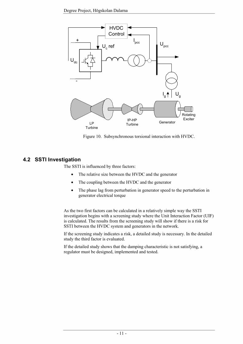
4.1 Description As mentioned above, when active equipments such as a Static Var Compensator (SVC) or an HVDC, influence a torsional mode it’s called SSTI. In the case of a series capacitor, the device causing the potential problem is a passive device, and thus modified operating practices and/or an active damping controller on the generating unit in question is needed to mitigate the problem. In the case of SSTI, however, the most effective solution is a careful control design. Figure 10 illustrates the concept of SSTI. A perturbation in the speed of the turbine-generator shaft will change the generator voltage phase position, and also the terminal voltage and current due to a change in flux linkage. The change at the generator terminals will change the a.c. bus voltage at the nearby HVDC terminal and by that influence the voltage and current in the HVDC converter. The converter control then acts to restore the d.c. voltage, a.c. voltage and a.c. current, leading to a change in the electrical torque on the turbine-generator shaft. Assuming a strong electrical coupling between the HVDC and the generator, it may be possible to have a phase relationship between the initial speed perturbation and the consequential perturbation in generator electrical torque that destabilizes one or more of the mechanical torsional modes. This of course is true only for those torsional modes in which the electrical generator participates. A closed loop therefore exists that involves the speed perturbation, resulting a.c. voltage perturbation, and the response of the HVDC converter and its controls to the a.c. voltage perturbation.


- 11 -

GeneratorIP-HPTurbineLP

Turbine

RotatingExciter

Ig Ug

UpccIpcc

Udc

+

-

Uc ref

HVDCControl

Figure 10. Subsynchronous torsional interaction with HVDC.

4.2 SSTI Investigation The SSTI is influenced by three factors:

• The relative size between the HVDC and the generator

• The coupling between the HVDC and the generator

• The phase lag from perturbation in generator speed to the perturbation in generator electrical torque

As the two first factors can be calculated in a relatively simple way the SSTI investigation begins with a screening study where the Unit Interaction Factor (UIF) is calculated. The results from the screening study will show if there is a risk for SSTI between the HVDC system and generators in the network.

If the screening study indicates a risk, a detailed study is necessary. In the detailed study the third factor is evaluated.

If the detailed study shows that the damping characteristic is not satisfying, a regulator must be designed, implemented and tested.


- 12 -

4.3 Screening Study The formula for UIF used in the screening study is developed in an EPRI study [7]:

2

1

−= −

tot

itot

i

HVDCi SC

SCMVA

MWUIF (6)

UIFi Unit interaction factor of the i:th unit MWHVDC MW rating of the HVDC system MVAi MVA rating of the i:th machine SCtot-i Short circuit capacity at the commutating bus excluding the i:th unit SCtot Short circuit capacity at the commutating bus including the i:th unit As seen from the formula the UIF depends on the rating between the HVDC system and the selected generator and also how much the generator contributes to the Short Circuit capacity (SC) on the bus were the HVDC is connected.

If the generator is radial connected to a HVDC converter station of equal size the UIF is 1.0.

If the MW rating of the HVDC is small compared to the generator the UIF will be close to zero. The other explanation for a UIF close to zero is large impedance (long distance) between the generator and the HVDC bus.

For HVDC Classic an UIF factor greater than 0.1 indicates that a detailed study might be necessary.

For HVDC Light, or more correctly, for a VSC there is no threshold value established.

4.4 Detailed Study The stability of torsional mechanical modes on the shaft of a turbine-generator is associated with the small-signal response of the system. Small-signal phenomena are most effectively analyzed by using either modal analysis or the measurement/calculation of damping and synchronizing torques. The disadvantage of modal analysis (or eigenanalysis) is that one needs to model both the mechanical and electrical systems in detail and to develop small-signal models for the system under study.

Damping torque analysis techniques, on the other hand, are based purely on analyzing the electrical component of the torque on the turbine-generator shaft for a wide range of frequencies in order to ensure stability over the entire range of torsional modes. This is a conservative approach, since the inherent mechanical damping is not taken into consideration.

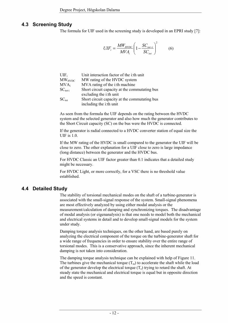
The damping torque analysis technique can be explained with help of Figure 11. The turbines give the mechanical torque (Tm) to accelerate the shaft while the load of the generator develop the electrical torque (Te) trying to retard the shaft. At steady state the mechanical and electrical torque is equal but in opposite direction and the speed is constant.


- 13 -

GeneratorIP-HP

TurbineLP

Turbine

Te

TmIP TmHPTmLP1

TmLP2

ω

Figure 11. Torques at the generator shaft. Consider a small perturbation in the speed (∆ω) that doesn’t affect the governor and thus the mechanical power. The speed perturbation changes the phase position of the output voltage from the generator and through that the electrical torque will be changed. The size of the change in the electrical torque will depend on the net connected to the generator. Mathematically this is expressed in (7) and (8). ω∆=∆ )(sFTe (7) )()()( ωω jSDsF += (8) F(s) in the equation is the transfer function for response from the generator, network, HVDC converter and HVDC control. The real part D(ω) of the transfer function is in phase with the initial speed perturbation. A positive D(ω) would increase the electrical torque when the speed increases and thus dampen the speed perturbation. In the detailed study the electrical damping for the subsynchronous frequencies is investigated using a single mass model of the generator. The electrical damping is defined according to (9). The details of the calculation are described in [6].

)Re(ω∆

∆= TeDe (9)

As mentioned above positive electrical damping indicates that rotor oscillations of the generator shaft are damped out. Negative electrical damping however, indicates that rotor oscillations are maintained or amplified which, depending of the magnitude of the oscillations, may cause great damage to the shaft. Some mechanical damping is always provided by the generator through bearing friction etc., but this is neglected. Therefore, when damping is mentioned in the following, it’s referred to the electrical damping.


- 14 -

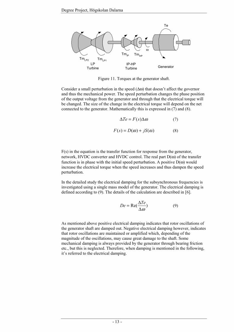
At the study a disturbance signal, which is continuously swept in frequency and amplitude, is injected in the speed order of the generator, se Figure 12. The change in electrical torque and the change in speed order are inputs to the damping calculation (9). The damping is then plotted against the frequency of the disturbance signal. The frequency is swept from 48 Hz to 1 Hz. As the results from low frequency disturbances requires longer time to stabilize, the shape of the sweep is a parable that allows fast sweeping for high frequencies and slow sweeping for low frequencies, se Figure 13.

19 20 21 22 23 24 25-4

-3

-2

-1

0

1

2

time (s)

spm

od (V

)

Speed modulation signal

Figure 12. Disturbance signal.


- 15 -

10 15 20 250

5

10

15

20

25

30

35

40

45

50Frequency sweep

time (s)

frequ

ency

(Hz)

Figure 13. The frequency sweep of the disturbance signal.

The circuit to simulate in the detailed study is two a.c. networks connected by a HVDC Light system. The HVDC system includes two converter stations and a d.c. cable. One of the a.c. networks includes the generator to be studied. More detail about the network is given in chapter 5.

The software used is PSCAD/EMTDC developed by Manitoba HVDC Research Center. PSCAD is the user interface to EMTDC where the power system to be simulated is defined. Code is generated from the symbols used in PSCAD, compiled and run in EMTDC. The control system for the converter is the same as used in real applications and presented in chapter 2.4.


- 16 -

5 A.C. System Representation during Simulation The HVDC Light transmission system is connected to two isolated a.c. systems. One a.c. system is represented by an infinite source behind an equivalent impedance. The SCR (11) of this system is 3. The other a.c. system includes a generator, as shown in Figure 14, in addition to a simplified a.c. network represented with an infinite source behind an equivalent impedance. In this study the HVDC Light station connected to the a.c. system without generator is called station 1. The HVDC Light station connected to the same bus as the generator is called station 2.

HVDC Light

Generator branch (GB)

Series impedanceBranch with infinite source (ISB)

L R

Com

mon

AC

bus

(P

CC

)

Converter transformer

G

Short line (xl)

STn SGn

xT xG

UGnU2n/U1n

Un

Figure 14. A.C. system with the generator to be study. The short circuit capacity on the common a.c. bus is defined in (10).

2

ZU

SCACbus = (10)

Where U= the actual line-to-line voltage Z= the short-circuit impedance The SCR is defined as the relation between the short circuit capacity on the common a.c. bus and the rating of the HVDC system:

HVDC

ACbus

MWSCSCR = (11)


- 17 -

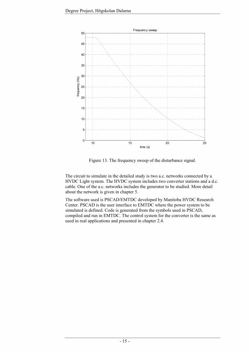
5.1 Calculation of Series Impedance for a Desired UIF To calculate the series impedance the short circuit power from the generator branch in Figure 14 must be calculated. The resistance of the transformer, generator and transmission line is neglected.

The impedance of the generator and transformer in ohm can be calculated as:

**2

1

22

=

n

n

Gn

GnGG U

USUxX (12)

* 22

Tn

nTT S

UxX = (13)

The short circuit power of the generator branch is:

***22

2

1

22

2

lTn

nT

n

n

Gn

GnG

nGB

XSUx

UU

SUx

USC

++

=⇒ (14)

If Gnn UU =1 and if the voltage drop over the line is neglected, nn UU =2 , the equation is reduced to:

**

22

2

lTn

nT

Gn

nG

nGB

XSUx

SUx

USC++

= (15)

Generator data

puxG 1780.0= kVUU nGn 8.131 == MVASGn 297= kVUU nn 1952 == => Ω= 79.22GX

Transformer data

154.0=Tx MVASTn 300= => Ω= 52.19TX

Line data

0=iX

Gives the short circuit power for the generator branch

=> MVASCGB 724.898=

The short circuit power from the branch with the infinite source can be calculated according to (16) as the ISBGBACbus SCSCSC +=


- 18 -

*

**1

H

G

GBH

G

ISB

MVAMVAUIF

SCMVAMVAUIF

SC

−

= (16)

Supposing that the power rating of HVDC (MVAH) is 354 MVA, the power rating of the generator (MVAG) is 297 MVA, it is then possible to calculate the short circuit power for the branch with the infinite source for a given UIF.

From the short circuit power and the voltage the equivalent impedance can be calculated (17).

ISBSCUZ = (17)

Supposing that the angle of the impedance is 83o the resistance and the inductance in Figure 14 can be calculated according to:

αcosZR = (18)

fZL

πα

2sin= (19)

The result from 9 different UIF is listed in Table 1. Yellow marked UIFs used in this study.

UIF

SC,ISB [MVA]

Z [ΩΩΩΩ]

R [ΩΩΩΩ]

X [ΩΩΩΩ]

L [H]

SCR

0.8 198.3 191.78 23.37 190.35 0.6059 3.10.7 274.0 138.77 16.91 137.74 0.4384 3.30.6 368.0 103.34 12.59 102.57 0.3265 3.60.5 488.9 77.78 9.48 77.20 0.2457 3.90.4 652.7 58.26 7.10 57.83 0.1841 4.40.3 892.7 42.60 5.19 42.28 0.1346 5.10.2 1.2953*103 29.36 3.58 29.14 0.0927 6.20.1 2.2040*103 17.25 2.10 17.12 0.0545 8.8

0.02 6.0393*103 6.30 0.77 6.25 0.0199 19.6

1.0 No AC source

Table 1. Values of the series impedance for different UIF.


- 19 -

6 Results The following plots are results from the cases specified in the study outline [1].

Table 2 in appendix 1 and table 3 in appendix 2 give the details about the studied cases.

The results reveal the impact from:

• short circuit ratio (SCR) of the AC network.

• machine load

• selected control modes of the VSC

• UIF

• active power, level and direction

• reactive power, level and direction

• capacitance at the d.c. side

It should be noted that the reactive power consumption by the series reactor L in Figure 14, would be changed when the inductance value is changed. This will lead to change of the voltage at PCC. In this study the voltage at PCC is kept constant by adjusting the infinite source voltage.

In all plots the x-axes show the frequency (Hz) and the y-axes the damping (pu).

Some values are given in per unit (pu) instead of absolute values. This means that the absolute values are normalized with respect to nominal or rated values.


- 20 -

6.1 Impact of A.C. Network Strength

6.1.1 General The aim of the control design is that the HVDC Light will contribute with positive damping. To be able to establish if that is the case, the damping characteristics for networks without HVDC Light are calculated. The damping characteristics are calculated for networks with different strengths in order see the strengths impact. To change the network strength, the series impedance in the a.c. network must be changed. This is described in chapter 5.1. These curves will be the references when analysing if the HVDC Light will contribute with positive damping, see Figure 20.

6.1.2 Comments Figure 15 shows the results obtained from cases with different network strength. SCR is defined in (11). The results show that there is a breakpoint around 35 Hz. Below the breakpoint the damping is more positive for stronger a.c. network and above, the damping is more positive for weaker a.c. network. Above the breakpoint the mechanical damping increases so this area is of less interest. The negative damping can be probably be referred to the machine itself, but why the damping for a weaker net becomes negative at a lower frequency compare to a stronger net, is not investigated.

5 10 15 20 25 30 35 40 45-1

-0.5

0

0.5

1

1.5

2

2.5

3

3.5

4Damping characteristics. Impact of a.c. network strength. Converter station not connected

Frequency (Hz)

De

(pu)

SCR = 3.6, UIF = 0.6 when converter connectedSCR = 4.4, UIF = 0.4 when converter connected SCR = 6.2, UIF = 0.2 when converter connectedSCR = 19.6, UIF = 0.02 when converter connected

Figure 15. Impact of a.c. network strength.


- 21 -

6.2 Impact of Machine Load

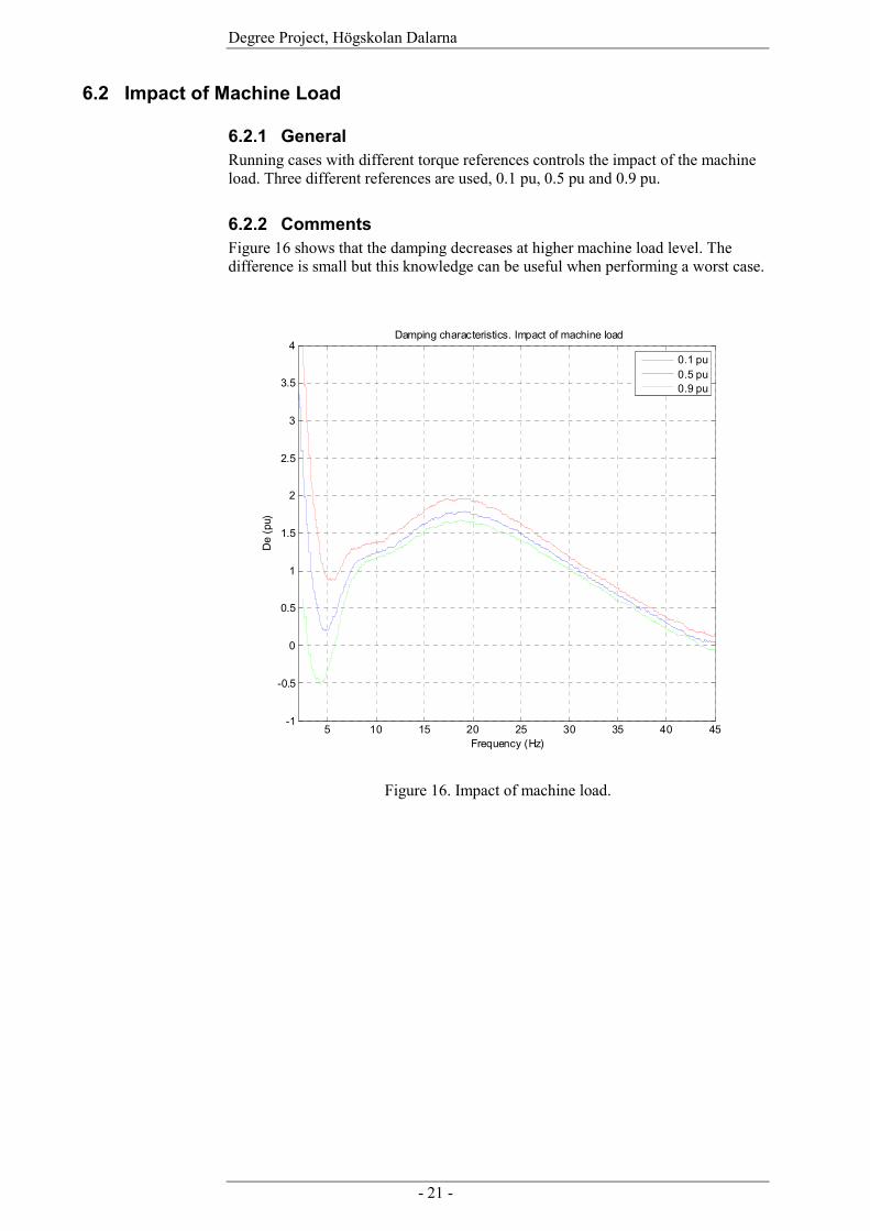
6.2.1 General Running cases with different torque references controls the impact of the machine load. Three different references are used, 0.1 pu, 0.5 pu and 0.9 pu.

6.2.2 Comments Figure 16 shows that the damping decreases at higher machine load level. The difference is small but this knowledge can be useful when performing a worst case.

5 10 15 20 25 30 35 40 45-1

-0.5

0

0.5

1

1.5

2

2.5

3

3.5

4Damping characteristics. Impact of machine load

Frequency (Hz)

De

(pu)

0.1 pu0.5 pu0.9 pu

Figure 16. Impact of machine load.


- 22 -

6.3 Impact of Control Modes

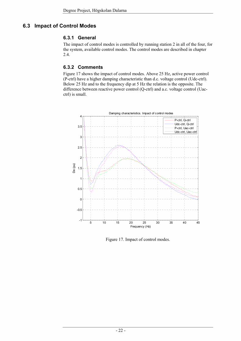
6.3.1 General The impact of control modes is controlled by running station 2 in all of the four, for the system, available control modes. The control modes are described in chapter 2.4.

6.3.2 Comments Figure 17 shows the impact of control modes. Above 25 Hz, active power control (P-ctrl) have a higher damping characteristic than d.c. voltage control (Udc-ctrl). Below 25 Hz and to the frequency dip at 5 Hz the relation is the opposite. The difference between reactive power control (Q-ctrl) and a.c. voltage control (Uac-ctrl) is small.

5 10 15 20 25 30 35 40 45-1

-0.5

0

0.5

1

1.5

2

2.5

3

3.5

4Damping characteristics. Impact of control modes

Frequency (Hz)

De

(pu)

P-ctrl, Q-ctrlUdc-ctrl, Q-ctrlP-ctrl, Uac-ctrlUdc-ctrl, Uac-ctrl

Figure 17. Impact of control modes.


- 23 -

6.4 Impact of UIF

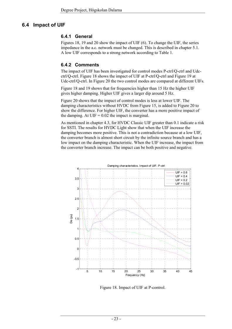
6.4.1 General Figures 18, 19 and 20 show the impact of UIF (6). To change the UIF, the series impedance in the a.c. network must be changed. This is described in chapter 5.1. A low UIF corresponds to a strong network according to Table 1.

6.4.2 Comments The impact of UIF has been investigated for control modes P-ctrl/Q-ctrl and Udc-ctrl/Q-ctrl. Figure 18 shows the impact of UIF at P-ctrl/Q-ctrl and Figure 19 at Udc-ctrl/Q-ctrl. In Figure 20 the two control modes are compared at different UIFs.

Figure 18 and 19 shows that for frequencies higher than 15 Hz the higher UIF gives higher damping. Higher UIF gives a larger dip around 5 Hz.

Figure 20 shows that the impact of control modes is less at lower UIF. The damping characteristics without HVDC from Figure 15, is added to Figure 20 to show the difference. For higher UIF, the converter has a more positive impact of the damping. At UIF = 0.02 the impact is marginal.

As mentioned in chapter 4.3, for HVDC Classic UIF greater than 0.1 indicate a risk for SSTI. The results for HVDC Light show that when the UIF increase the damping becomes more positive. This is not a contradiction because at a low UIF, the converter branch is almost short circuit by the infinite source branch and has a low impact on the damping characteristic. When the UIF increase, the impact from the converter branch increase. The impact can be both positive and negative.

5 10 15 20 25 30 35 40 45-1

-0.5

0

0.5

1

1.5

2

2.5

3

3.5

4Damping characteristics. Impact of UIF. P-ctrl

Frequency (Hz)

De

(pu)

UIF = 0.6UIF = 0.4UIF = 0.2UIF = 0.02

Figure 18. Impact of UIF at P-control.


- 24 -

5 10 15 20 25 30 35 40 45-1

-0.5

0

0.5

1

1.5

2

2.5

3

3.5

4Damping characteristics. Impact of UIF. Udc ctrl

Frequency (Hz)

De

(pu)

UIF = 0.6UIF = 0.4UIF = 0.2UIF = 0.02

Figure 19. Impact of UIF at Udc-control.

10 20 30 40-1

0

1

2

3

4UIF = 0.6

Without HVDC

P-ctrl

Udc-ctrl

10 20 30 40-1

0

1

2

3

4UIF = 0.4

10 20 30 40-1

0

1

2

3

4UIF = 0.2

10 20 30 40-1

0

1

2

3

4UIF = 0.02

Figure 20. P-ctrl and Udc-ctrl at different UIFs.


- 25 -

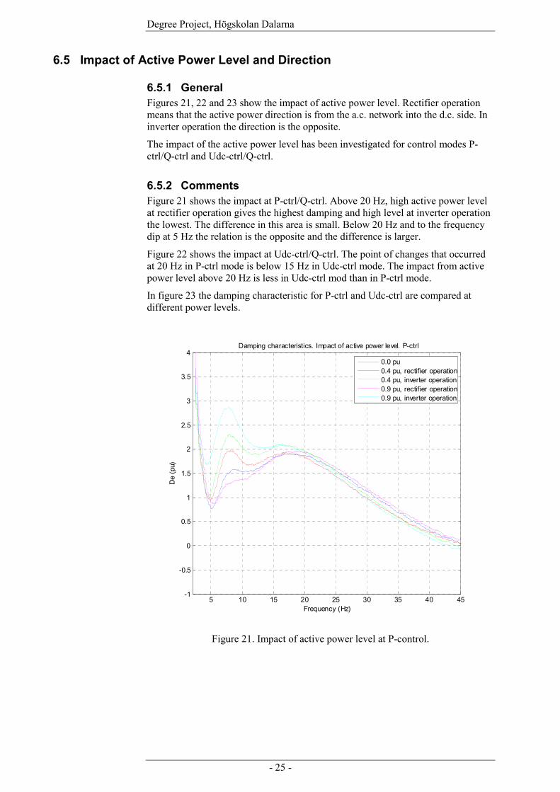
6.5 Impact of Active Power Level and Direction

6.5.1 General Figures 21, 22 and 23 show the impact of active power level. Rectifier operation means that the active power direction is from the a.c. network into the d.c. side. In inverter operation the direction is the opposite.

The impact of the active power level has been investigated for control modes P-ctrl/Q-ctrl and Udc-ctrl/Q-ctrl.

6.5.2 Comments Figure 21 shows the impact at P-ctrl/Q-ctrl. Above 20 Hz, high active power level at rectifier operation gives the highest damping and high level at inverter operation the lowest. The difference in this area is small. Below 20 Hz and to the frequency dip at 5 Hz the relation is the opposite and the difference is larger.

Figure 22 shows the impact at Udc-ctrl/Q-ctrl. The point of changes that occurred at 20 Hz in P-ctrl mode is below 15 Hz in Udc-ctrl mode. The impact from active power level above 20 Hz is less in Udc-ctrl mod than in P-ctrl mode.

In figure 23 the damping characteristic for P-ctrl and Udc-ctrl are compared at different power levels.

5 10 15 20 25 30 35 40 45-1

-0.5

0

0.5

1

1.5

2

2.5

3

3.5

4Damping characteristics. Impact of active power level. P-ctrl

Frequency (Hz)

De

(pu)

0.0 pu0.4 pu, rectifier operation0.4 pu, inverter operation0.9 pu, rectifier operation0.9 pu, inverter operation

Figure 21. Impact of active power level at P-control.


- 26 -

5 10 15 20 25 30 35 40 45-1

-0.5

0

0.5

1

1.5

2

2.5

3

3.5

4Damping characteristics. Impact of active power level. Udc ctrl

Frequency (Hz)

De

(pu)

0.0 pu0.4 pu, rectifier operation0.4 pu, inverter operation0.9 pu, rectifier operation0.9 pu, inverter operation

Figure 22. Impact of active power level at Udc-control.

10 20 30 40-1

0

1

2

3

4P = 0.0 pu

Pctrl

Udcctrl

10 20 30 40-1

0

1

2

3

4P = 0.4 pu, rectifier operation.

10 20 30 40-1

0

1

2

3

4P = 0.4 pu, inverter operation.

10 20 30 40-1

0

1

2

3

4P = 0.9 pu, rectifier operation.

10 20 30 40-1

0

1

2

3

4P = 0.9 pu, inverter operation.

Figure 23 P-control and Udc-control at different power level.


- 27 -

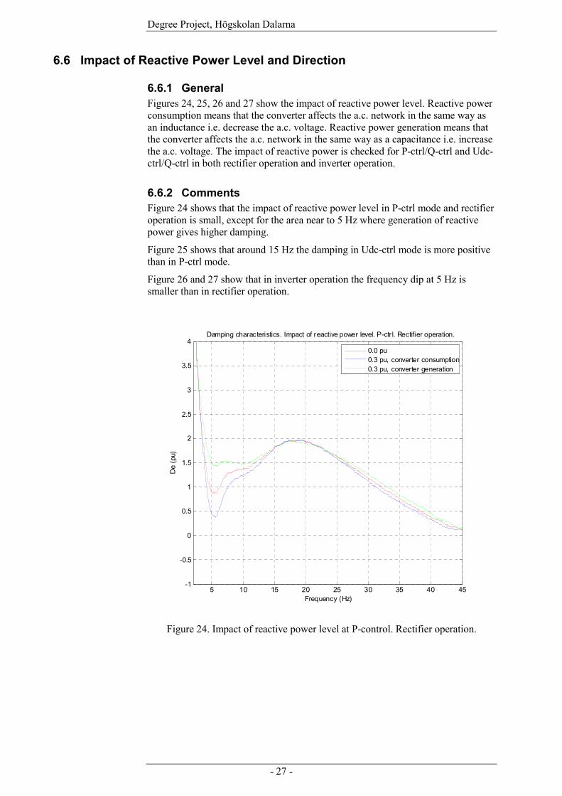
6.6 Impact of Reactive Power Level and Direction

6.6.1 General Figures 24, 25, 26 and 27 show the impact of reactive power level. Reactive power consumption means that the converter affects the a.c. network in the same way as an inductance i.e. decrease the a.c. voltage. Reactive power generation means that the converter affects the a.c. network in the same way as a capacitance i.e. increase the a.c. voltage. The impact of reactive power is checked for P-ctrl/Q-ctrl and Udc-ctrl/Q-ctrl in both rectifier operation and inverter operation.

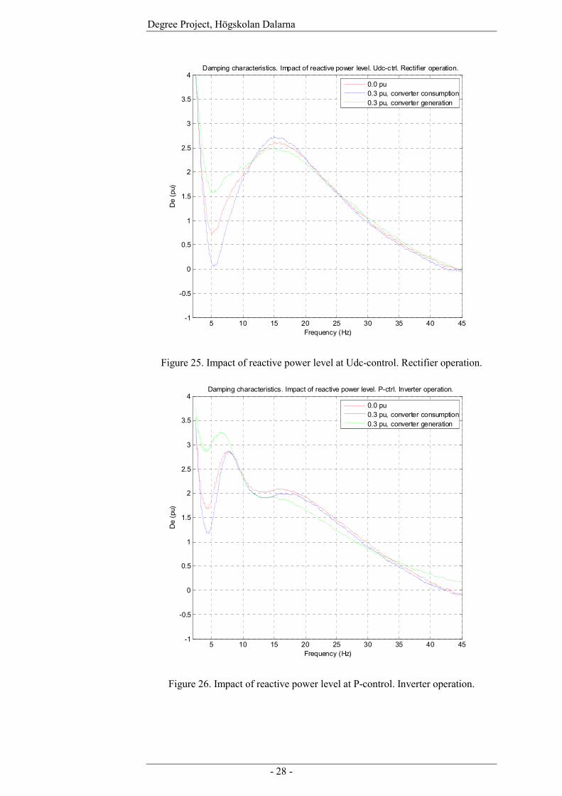
6.6.2 Comments Figure 24 shows that the impact of reactive power level in P-ctrl mode and rectifier operation is small, except for the area near to 5 Hz where generation of reactive power gives higher damping.

Figure 25 shows that around 15 Hz the damping in Udc-ctrl mode is more positive than in P-ctrl mode.

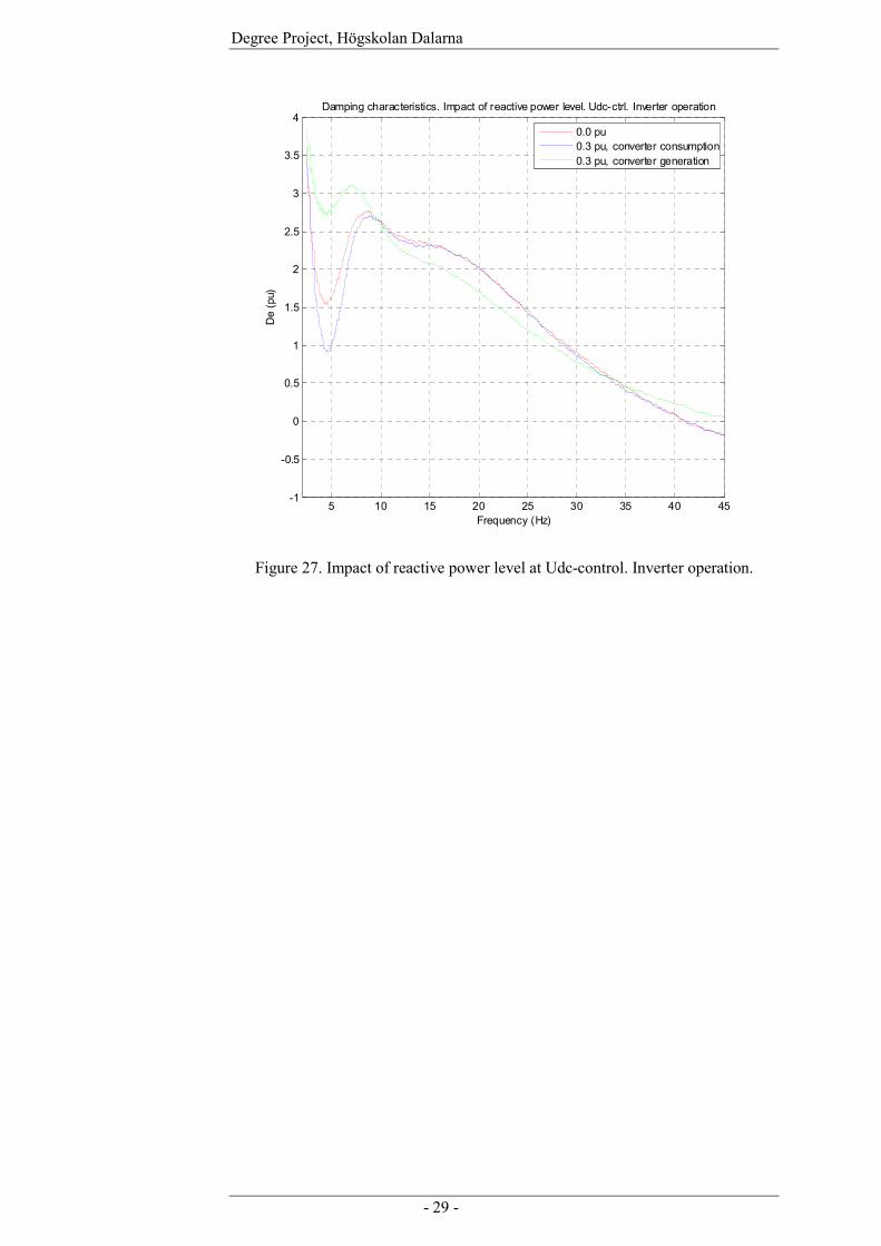
Figure 26 and 27 show that in inverter operation the frequency dip at 5 Hz is smaller than in rectifier operation.

5 10 15 20 25 30 35 40 45-1

-0.5

0

0.5

1

1.5

2

2.5

3

3.5

4Damping characteristics. Impact of reactive power level. P-ctr l. Rectifier operation.

Frequency (Hz)

De

(pu)

0.0 pu0.3 pu, converter consumption0.3 pu, converter generation

Figure 24. Impact of reactive power level at P-control. Rectifier operation.


- 28 -

5 10 15 20 25 30 35 40 45-1

-0.5

0

0.5

1

1.5

2

2.5

3

3.5

4Damping characteristics. Impact of reactive power level. Udc-ctrl. Rectifier operation.

Frequency (Hz)

De

(pu)


Figure 25. Impact of reactive power level at Udc-control. Rectifier operation.

5 10 15 20 25 30 35 40 45-1

-0.5

0

0.5

1

1.5

2

2.5

3

3.5

4Damping characteristics. Impact of reactive power level. P-ctrl. Inverter operation.

Frequency (Hz)

De

(pu)


Figure 26. Impact of reactive power level at P-control. Inverter operation.


- 29 -

5 10 15 20 25 30 35 40 45-1

-0.5

0

0.5

1

1.5

2

2.5

3

3.5

4Damping characteristics. Impact of reactive power level. Udc-ctrl. Inverter operation

Frequency (Hz)

De

(pu)


Figure 27. Impact of reactive power level at Udc-control. Inverter operation.


- 30 -

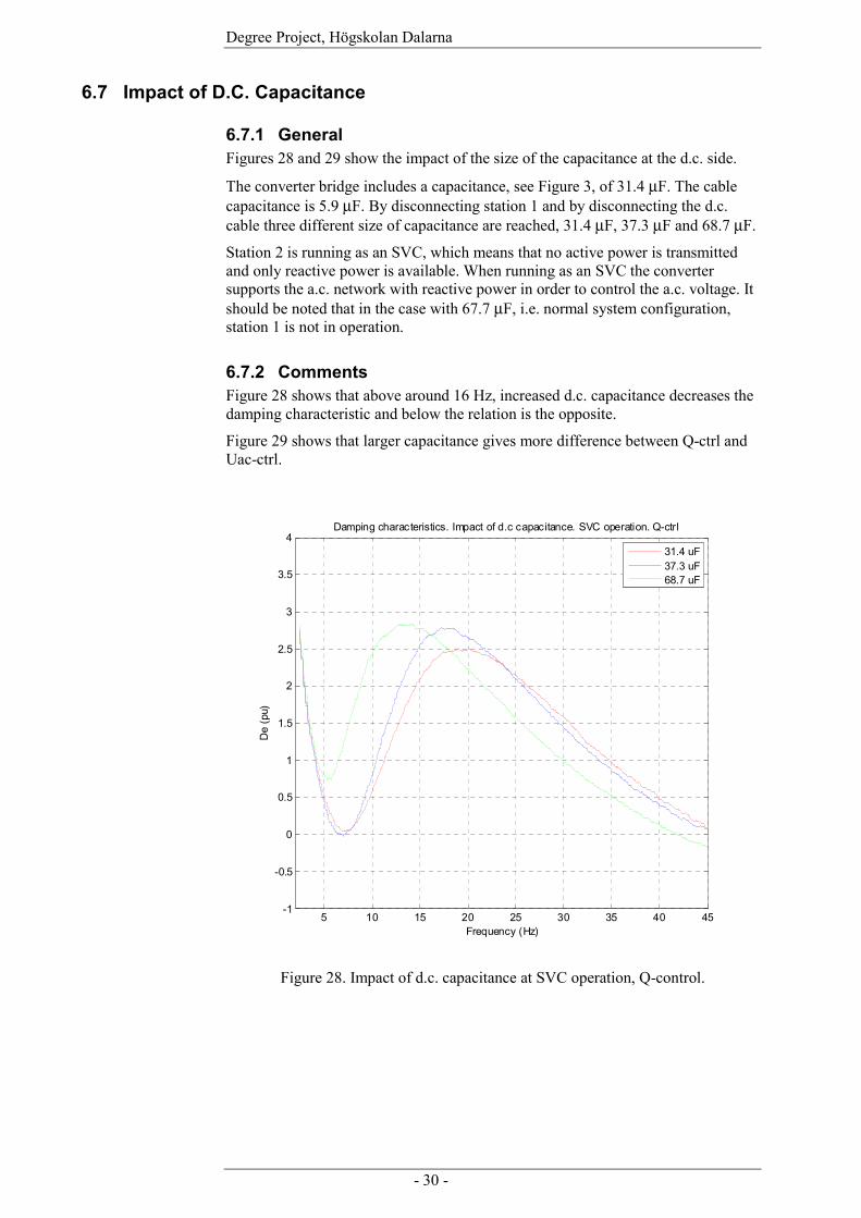
6.7 Impact of D.C. Capacitance

6.7.1 General Figures 28 and 29 show the impact of the size of the capacitance at the d.c. side.

The converter bridge includes a capacitance, see Figure 3, of 31.4 µF. The cable capacitance is 5.9 µF. By disconnecting station 1 and by disconnecting the d.c. cable three different size of capacitance are reached, 31.4 µF, 37.3 µF and 68.7 µF.

Station 2 is running as an SVC, which means that no active power is transmitted and only reactive power is available. When running as an SVC the converter supports the a.c. network with reactive power in order to control the a.c. voltage. It should be noted that in the case with 67.7 µF, i.e. normal system configuration, station 1 is not in operation.

6.7.2 Comments Figure 28 shows that above around 16 Hz, increased d.c. capacitance decreases the damping characteristic and below the relation is the opposite.

Figure 29 shows that larger capacitance gives more difference between Q-ctrl and Uac-ctrl.

5 10 15 20 25 30 35 40 45-1

-0.5

0

0.5

1

1.5

2

2.5

3

3.5

4Damping characteristics. Impact of d.c capacitance. SVC operation. Q-ctrl

Frequency (Hz)

De

(pu)

31.4 uF37.3 uF68.7 uF

Figure 28. Impact of d.c. capacitance at SVC operation, Q-control.


- 31 -

5 10 15 20 25 30 35 40 45-1

-0.5

0

0.5

1

1.5

2

2.5

3

3.5

4Damping characteristics. Impact of d.c capacitance. SVC operation. Uac-ctrl.

Frequency (Hz)

De

(pu)

31.4 uF37.3 uF68.7 uF

Figure 29. Impact of d.c. capacitance at SVC operation, Uac-control.


- 32 -

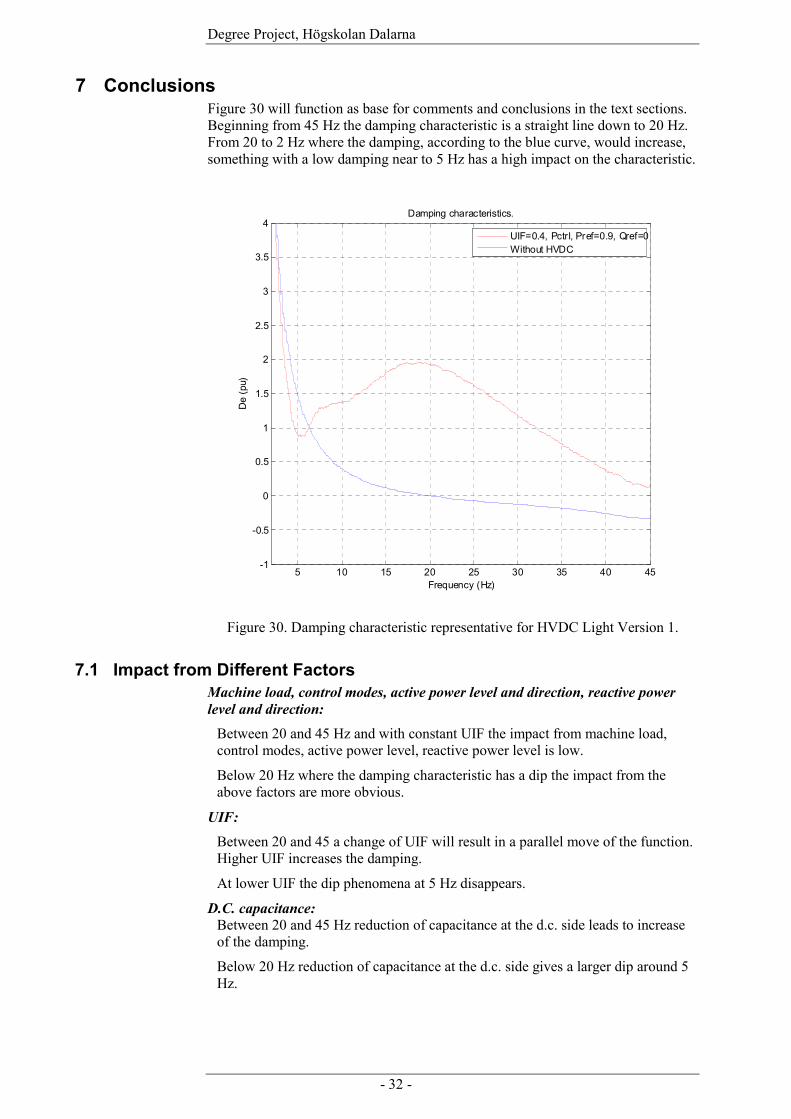
7 Conclusions Figure 30 will function as base for comments and conclusions in the text sections. Beginning from 45 Hz the damping characteristic is a straight line down to 20 Hz. From 20 to 2 Hz where the damping, according to the blue curve, would increase, something with a low damping near to 5 Hz has a high impact on the characteristic.

5 10 15 20 25 30 35 40 45-1

-0.5

0

0.5

1

1.5

2

2.5

3

3.5

4Damping characteristics.

Frequency (Hz)

De

(pu)

UIF=0.4, Pctrl, Pref=0.9, Qref=0Without HVDC

Figure 30. Damping characteristic representative for HVDC Light Version 1.

7.1 Impact from Different Factors Machine load, control modes, active power level and direction, reactive power level and direction:

Between 20 and 45 Hz and with constant UIF the impact from machine load, control modes, active power level, reactive power level is low.

Below 20 Hz where the damping characteristic has a dip the impact from the above factors are more obvious.

UIF: Between 20 and 45 a change of UIF will result in a parallel move of the function. Higher UIF increases the damping.

At lower UIF the dip phenomena at 5 Hz disappears.

D.C. capacitance: Between 20 and 45 Hz reduction of capacitance at the d.c. side leads to increase of the damping.

Below 20 Hz reduction of capacitance at the d.c. side gives a larger dip around 5 Hz.


- 33 -

7.2 Comparison with Operation without HVDC Light Figure 20 illustrates the differences at operation with and without HVDV Light.

At UIF 0.6 corresponding to SCR 3.6 the HVDC increase the damping between 7 Hz to 45 Hz. When UIF decrease, SCR increase, the cross point at 7 Hz moves against a higher value. At UIF 0.2 corresponding to SCR 6.2 the point is around 9 Hz but the damping below 9 Hz is now more positive. At UIF 0.02 corresponding to SCR 19.6 the cross point is around 20 Hz. The damping below 20 Hz is positive and only decreased in a minor way.

7.3 General Conclusion To summarize, the conclusion is that HVDC Light increases the damping characteristic in the frequency range of interest.

8 References. [1] Ying Jiang Häfner, “SSTI Study Outline.”, 1JNL100098-155 Rev. 01 [2] Ying Jiang Häfner, “Exam Work Specification for SSTI study.”, 05TST0048 [3] M. Speychal, “SSTI Investigation for the HVDC Light B Concept.”, 1JNL100051-911 [4] Thomas Tulkiewicz, “SSTI characteristics of HVDC Light.”, 1JNL100095-527 [5] Thomas Tulkiewicz, “SSTI Characteristics of HVDC Light.”, 1JNL100096-916

[6] Paulo Fisher, “Extracting Oscillating Phasor using a method derived from Recursive Least Square algorithm.”, 04TST0521

[7] Electric Power Institute, “HVDC Systems Control for Damping of Subsynchronous Oscillations”, EPRI EL-2708, Final report October 1982

[8] www.abb.com, “HVDC Light”


- 34 -

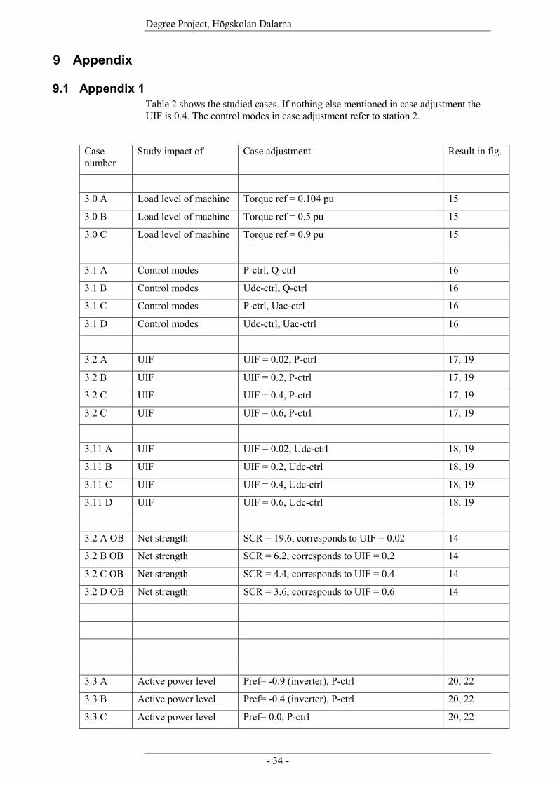
9 Appendix

9.1 Appendix 1 Table 2 shows the studied cases. If nothing else mentioned in case adjustment the UIF is 0.4. The control modes in case adjustment refer to station 2.

Case number

Study impact of Case adjustment Result in fig.

3.0 A Load level of machine Torque ref = 0.104 pu 15

3.0 B Load level of machine Torque ref = 0.5 pu 15

3.0 C Load level of machine Torque ref = 0.9 pu 15

3.1 A Control modes P-ctrl, Q-ctrl 16

3.1 B Control modes Udc-ctrl, Q-ctrl 16

3.1 C Control modes P-ctrl, Uac-ctrl 16

3.1 D Control modes Udc-ctrl, Uac-ctrl 16

3.2 A UIF UIF = 0.02, P-ctrl 17, 19

3.2 B UIF UIF = 0.2, P-ctrl 17, 19

3.2 C UIF UIF = 0.4, P-ctrl 17, 19

3.2 C UIF UIF = 0.6, P-ctrl 17, 19

3.11 A UIF UIF = 0.02, Udc-ctrl 18, 19

3.11 B UIF UIF = 0.2, Udc-ctrl 18, 19

3.11 C UIF UIF = 0.4, Udc-ctrl 18, 19

3.11 D UIF UIF = 0.6, Udc-ctrl 18, 19

3.2 A OB Net strength SCR = 19.6, corresponds to UIF = 0.02 14

3.2 B OB Net strength SCR = 6.2, corresponds to UIF = 0.2 14

3.2 C OB Net strength SCR = 4.4, corresponds to UIF = 0.4 14

3.2 D OB Net strength SCR = 3.6, corresponds to UIF = 0.6 14

3.3 A Active power level Pref= -0.9 (inverter), P-ctrl 20, 22

3.3 B Active power level Pref= -0.4 (inverter), P-ctrl 20, 22

3.3 C Active power level Pref= 0.0, P-ctrl 20, 22


- 35 -

3.3 D Active power level Pref= 0.4 (rectifier), P-ctrl 20, 22

3.3 E Active power level Pref= 0.9 (rectifier), P-ctrl 20, 22

3.4 A Active power level Pref= -0.9 (inverter), Udc-ctrl 21, 22

3.4 B Active power level Pref= -0.4 (inverter), Udc-ctrl 21, 22

3.4 C Active power level Pref= 0.0, Udc-ctrl 21, 22

3.4 D Active power level Pref= 0.4 (rectifier), Udc-ctrl 21, 22

3.4 E Active power level Pref= 0.9 (rectifier), Udc-ctrl 21, 22

3.5 A Reactive power level Qref = -0.3 (conv. consumption), P-ctrl, rec 23

3.5 B Reactive power level Qref = 0.0, P-ctrl, rec 23

3.5 C Reactive power level Qref = 0.3 (conv. generation), P-ctrl, rec 23

3.6 A Reactive power level Qref = -0.3 (conv. consumption), Udc-ctrl, rec 24

3.6 B Reactive power level Qref = 0.0, Udc-ctrl, rec 24

3.6 C Reactive power level Qref = 0.3 (conv. generation), Udc-ctrl, rec 24

3.7 A Reactive power level Qref = -0.3 (conv. consumption), P-ctrl, inv 25

3.7 B Reactive power level Qref = 0.0, P-ctrl, inv 25

3.7 C Reactive power level Qref = 0.3 (conv. generation), P-ctrl, inv 25

3.8 A Reactive power level Qref = -0.3 (conv. consumption), Udc-ctrl, inv 26

3.8 B Reactive power level Qref = 0.0, Udc-ctrl, inv 26

3.8 C Reactive power level Qref = 0.3 (conv. generation), Udc-ctrl, inv 26

3.9 A D.C capacitance. D.C cable disconnected, Q-ctrl 27

3.9 B D.C capacitance. Other station disconnected, Q-ctrl 27

3.9 C D.C capacitance. Normal config., Q-ctrl 27

3.10 A D.C capacitance. D.C cable disconnected, Uac-ctrl 28

3.10 B D.C capacitance. Other station disconnected, Uac-ctrl 28

3.10 C D.C capacitance. Normal config., Uac-ctrl 28

Spec. case A

Switching method (control speed)

PWM method = 3PWM 29

Table 2. Case specification.


- 36 -

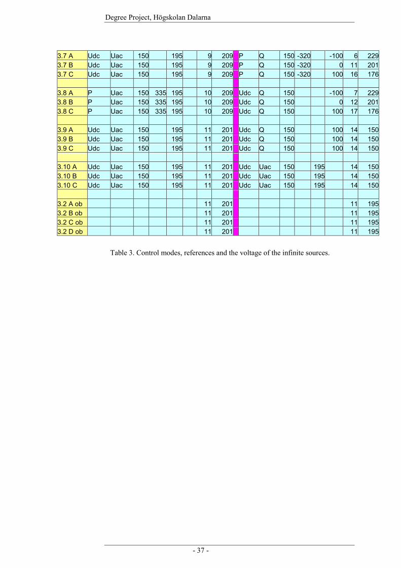
9.2 Appendix 2 Table 3 shows the control modes, references and voltage of the infinite sources for the studied cases. A positive sign for the active power reference (Pref) means that the active power direction will be from the station that controls the active power to the station controlling the d.c. voltage. For example in case 3.0 A the active power direction is from station 2 to station 1.

Station1 Station 2 CASE P/Udc Q/Uac Udc P Uac Q TCP Uac is P/Udc Q/Uac Udc P Uac Q TCP Uac is ref. ref. ref. ref. ref. ref. ref. ref. 3.0 A Udc Uac 150 195 11 201 P Q 150 320 0 10 2113.0 B Udc Uac 150 195 11 201 P Q 150 320 0 10 2043.0 C Udc Uac 150 195 11 201 P Q 150 320 0 10 201 3.1 A Udc Uac 150 195 11 201 P Q 150 320 0 10 2113.1 B P Uac 150 -300 195 9 201 Udc Q 150 0 10 2113.1 C Udc Uac 150 195 11 201 P Uac 150 320 195 10 2113.1 D P Uac 150 -300 195 9 201 Udc Uac 150 195 10 213 3.2 A Udc Uac 150 195 11 201 P Q 150 330 0 10 1953.2 B Udc Uac 150 195 11 201 P Q 150 320 0 10 1993.2 C Udc Uac 150 195 11 201 P Q 150 320 0 10 2113.2 D Udc Uac 150 195 11 201 P Q 150 330 0 11 246 3.11 A P Uac 150 -300 195 10 201 Udc Q 150 0 9 1953.11 B P Uac 150 -300 195 10 201 Udc Q 150 0 9 1993.11 C P Uac 150 -300 195 9 201 Udc Q 150 0 10 2113.11 D P Uac 150 -300 195 10 201 Udc Q 150 0 9 246 3.3 A Udc Uac 150 195 9 209 P Q 150 -320 0 11 2013.3 B Udc Uac 150 195 8 201 P Q 150 -140 0 9 1873.3 C Udc Uac 150 195 8 201 P Q 150 0 0 9 1873.3 D Udc Uac 150 195 10 201 P Q 150 140 0 10 1933.3 E Udc Uac 150 195 11 201 P Q 150 320 0 10 211 3.4 A P Uac 150 335 195 10 209 Udc Q 150 0 12 2013.4 B P Uac 150 155 195 9 201 Udc Q 150 0 10 1863.4 C P Uac 150 0 195 7 201 Udc Q 150 0 9 1853.4 D P Uac 150 -130 195 7 201 Udc Q 150 0 8 1923.4 E P Uac 150 195 11 201 Udc Q 150 0 10 211 3.5 A Udc Uac 150 195 10 201 P Q 150 320 -100 5 2353.5 B Udc Uac 150 195 11 201 P Q 150 320 0 10 2113.5 C Udc Uac 150 195 11 201 P Q 150 320 100 15 185 3.6 A P Uac 150 -300 195 11 201 Udc Q 150 -100 5 2353.6 B P Uac 150 0 195 11 201 Udc Q 150 0 10 2113.6 C P Uac 150 -300 195 8 209 Udc Q 150 100 15 185


- 37 -

3.7 A Udc Uac 150 195 9 209 P Q 150 -320 -100 6 2293.7 B Udc Uac 150 195 9 209 P Q 150 -320 0 11 2013.7 C Udc Uac 150 195 9 209 P Q 150 -320 100 16 176 3.8 A P Uac 150 335 195 10 209 Udc Q 150 -100 7 2293.8 B P Uac 150 335 195 10 209 Udc Q 150 0 12 2013.8 C P Uac 150 335 195 10 209 Udc Q 150 100 17 176 3.9 A Udc Uac 150 195 11 201 Udc Q 150 100 14 1503.9 B Udc Uac 150 195 11 201 Udc Q 150 100 14 1503.9 C Udc Uac 150 195 11 201 Udc Q 150 100 14 150 3.10 A Udc Uac 150 195 11 201 Udc Uac 150 195 14 1503.10 B Udc Uac 150 195 11 201 Udc Uac 150 195 14 1503.10 C Udc Uac 150 195 11 201 Udc Uac 150 195 14 150 3.2 A ob 11 201 11 1953.2 B ob 11 201 11 1953.2 C ob 11 201 11 1953.2 D ob 11 201 11 195

Table 3. Control modes, references and the voltage of the infinite sources.

Studie av subsynkron interaktion (SSTI) mellan ett HVDC ...518005/FULLTEXT01.pdf · torsional...

Documents

Transcript of Studie av subsynkron interaktion (SSTI) mellan ett HVDC ...518005/FULLTEXT01.pdf · torsional...