AFRL-OSR-VA-TR-2014-0120

ADVANCING THE SURVEILLANCE CAPABILITIES OF THE AIR FORCES LARGE-APERATURE TELESCOPES

Stuart JefferiesUNIVERSITY OF HAWAII SYSTEMS HONOLULU

Final Report03/06/2014

DISTRIBUTION A: Distribution approved for public release.

AF Office Of Scientific Research (AFOSR)/ RTBArlington, Virginia 22203

Air Force Research Laboratory

Air Force Materiel Command

REPORT DOCUMENTATION PAGE Form ApprovedOMB No. 0704-0188

1. REPORT DATE (DD-MM-YYYY) 2. REPORT TYPE

4. TITLE AND SUBTITLE 5a. CONTRACT NUMBER

6. AUTHOR(S)

7. PERFORMING ORGANIZATION NAME(S) AND ADDRESS(ES)

9. SPONSORING/MONITORING AGENCY NAME(S) AND ADDRESS(ES)

8. PERFORMING ORGANIZATION REPORT NUMBER

10. SPONSOR/MONITOR'S ACRONYM(S)

13. SUPPLEMENTARY NOTES

12. DISTRIBUTION/AVAILABILITY STATEMENT

14. ABSTRACT

15. SUBJECT TERMS

18. NUMBER OF PAGES

19a. NAME OF RESPONSIBLE PERSON a. REPORT b. ABSTRACT c. THIS PAGE

17. LIMITATION OF ABSTRACT

Standard Form 298 (Rev. 8/98)Prescribed by ANSI Std. Z39.18

Adobe Professional 7.0

PLEASE DO NOT RETURN YOUR FORM TO THE ABOVE ORGANIZATION. 3. DATES COVERED (From - To)

5b. GRANT NUMBER

5c. PROGRAM ELEMENT NUMBER

5d. PROJECT NUMBER

5e. TASK NUMBER

5f. WORK UNIT NUMBER

11. SPONSOR/MONITOR'S REPORT NUMBER(S)

16. SECURITY CLASSIFICATION OF:

19b. TELEPHONE NUMBER (Include area code)

The public reporting burden for this collection of information is estimated to average 1 hour per response, including the time for reviewing instructions, searching existing data sources, gathering andmaintaining the data needed, and completing and reviewing the collection of information. Send comments regarding this burden estimate or any other aspect of this collection of information, includingsuggestions for reducing the burden, to the Department of Defense, Executive Service Directorate (0704-0188). Respondents should be aware that notwithstanding any other provision of law, noperson shall be subject to any penalty for failing to comply with a collection of information if it does not display a currently valid OMB control number.

  1  

ADVANCING THE SURVEILLANCE CAPABILITIES OF THE AIR FORCE'S LARGE-APERATURE TELESCOPES

AFOSR Award: FA9550-09-1-0216

Executive Summary

The Air Force’s 3-meter class AEOS and Starfire telescopes play a critical role in the detection and imaging of objects in the near-Earth environment for space situational awareness (SSA). Ideally these assets provide horizon-to-horizon surveillance of the sky, twenty-four hours a day, seven days a week. In practice, the amount of sky over which we can obtain high-resolution images of space objects is limited to regions where the combination of adaptive optics (AO) compensation and numerical image restoration are effective. For current AO systems and image processing techniques this requires benign to moderate turbulence conditions which results in a serious reduction in both the area of sky that can be monitored and the time it can be monitored. Moreover, it adversely impacts our capability for surveillance of some types of satellites (e.g., low-orbit, sun-synchronous satellites). We demonstrate that by improving the synergy between the data acquisition and processing steps, and leveraging the information on the temporal behavior of the atmosphere that is encoded in the AO wave front sensor data, we can achieve high-resolution imaging through much stronger atmospheric turbulence than is possible with current imaging systems. The proposed approach captures images using a range of aperture sizes and then uses a bootstrap restoration process that starts with the smallest aperture data. This technique provides a trajectory through the parameter hyperspace in the restoration that is less susceptible to entrapment in local minima than is encountered with the traditional approach of restoring single aperture data. Implementing the proposed approach has the potential to provide a six-fold increase in the spatial and temporal coverage of the sky: a significant advance for SSA. People Involved in Research: Dr. S. M. Jefferies and Dr. D. A. Hope Publications:

1. Hope, D. A., Jefferies, S. M., Hart, M. and Nagy, J. G. 2014, “High-resolution image restoration through strong atmospheric turbulence”, Optics Express, in review

2. Chu, Q., Jefferies, S. M. and Nagy, J. D.: 2013, “Iterative wave front reconstruction for astronomical imaging”, SIAM J. on Sci. Computing, S84-S103

3. Jefferies, S. M., Hope, D., Hart, M. and Nagy, J. 2013, “High-resolution imaging through strong atmospheric turbulence and over wide fields of view”, Proceedings of the Advanced Maui Optical and Space Surveillance Technologies Conference, held in Wailea, Maui, September 2013, Ed: S. Ryan, The Maui Economic Development Board, p.545

4. Jefferies, S. M., Hope, D., Hart, M. and Nagy, J. 2013, “High resolution imaging through strong atmospheric turbulence and over wide fields of view”, Proc. SPIE 8890, Remote Sensing of Clouds and the Atmosphere XVIII; and Optics in Atmospheric Propagation and Adaptive Systems XVI, 88901C

  2  

5. Jefferies, S. M., Hope, D., Hart, M. and Nagy, J. 2013, “Imaging through atmospheric turbulence using aperture diversity and blind deconvolution”, OSA topical meeting on Computational Optical Sensing and Imaging, Computational Imaging through Turbulence and Scattering Media, paper Cth1B.1

6. Jefferies, S. M. and Hart, M. 2011, “Deconvolution from wave front sensing using the frozen flow hypothesis”, Optics Express, 19, 1975-1984

7. Hope, D. A. et al. 2012, "Numerical restoration of imagery obtained in strong turbulence," in Computational Optical Sensing and Imaging, OSA Technical Digest (online) (OSA, 2012), paper CTu2B.1.

8. Vorontsov S. V., Strakhov, V. N., Jefferies S. M. and Borelli, K. J. 2011, “Deconvolution of astronomical images using SOR with adaptive relaxation”, Optics Express, 19, 13509-13524

9. Hope, D. A. and Jefferies, S. M. 2011, “Compact multi-frame blind deconvolution”, Optics Letters, 36, 867-869

10. Hope, D. A and Jefferies, S. M. 2011, “Multi-frame blind deconvolution: compact and multi-channel versions”, Proceedings of the Advanced Maui Optical and Space Surveillance Technologies Conference, held in Wailea, Maui, September 2011, Ed: S. Ryan, The Maui Economic Development Board, p. E39

11. Jefferies, S., Hart, M., Hope, D., Hege, E. K., Briguglio, R., Pinna, E., Puglisi, A., Quiros, F. and Xompero, M. 2011, “Multi-frame myopic deconvolution for imaging in daylight and strong turbulence conditions”, Proceedings of the Advanced Maui Optical and Space Surveillance Technologies Conference, held in Wailea, Maui, September 2011, Ed: S. Ryan, The Maui Economic Development Board, p. E40

12. Hart, M., Jefferies, S., Hope, D., Hege, E. K., Briguglio, R., Pinna, E., Puglisi, A., Quiros, F. and Xompero, M. 2011, “Multi-frame blind deconvolution for imaging in daylight and strong turbulence conditions”, Unconventional imaging, wavefront sensing, and adaptive coded aperture imaging and non-imaging sensor systems, Proc. SPIE 8265, 8165A-21

13. Nagy, J., Jefferies, S. and Chu, Q. 2010, “Fast PSF reconstruction using the frozen flow hypothesis”, Proceedings of the Advanced Maui Optical and Space Surveillance Technologies Conference, held in Wailea, Maui, Hawaii, September 2010, Ed: S. Ryan, The Maui Economic Development Board, p. E57

  3  

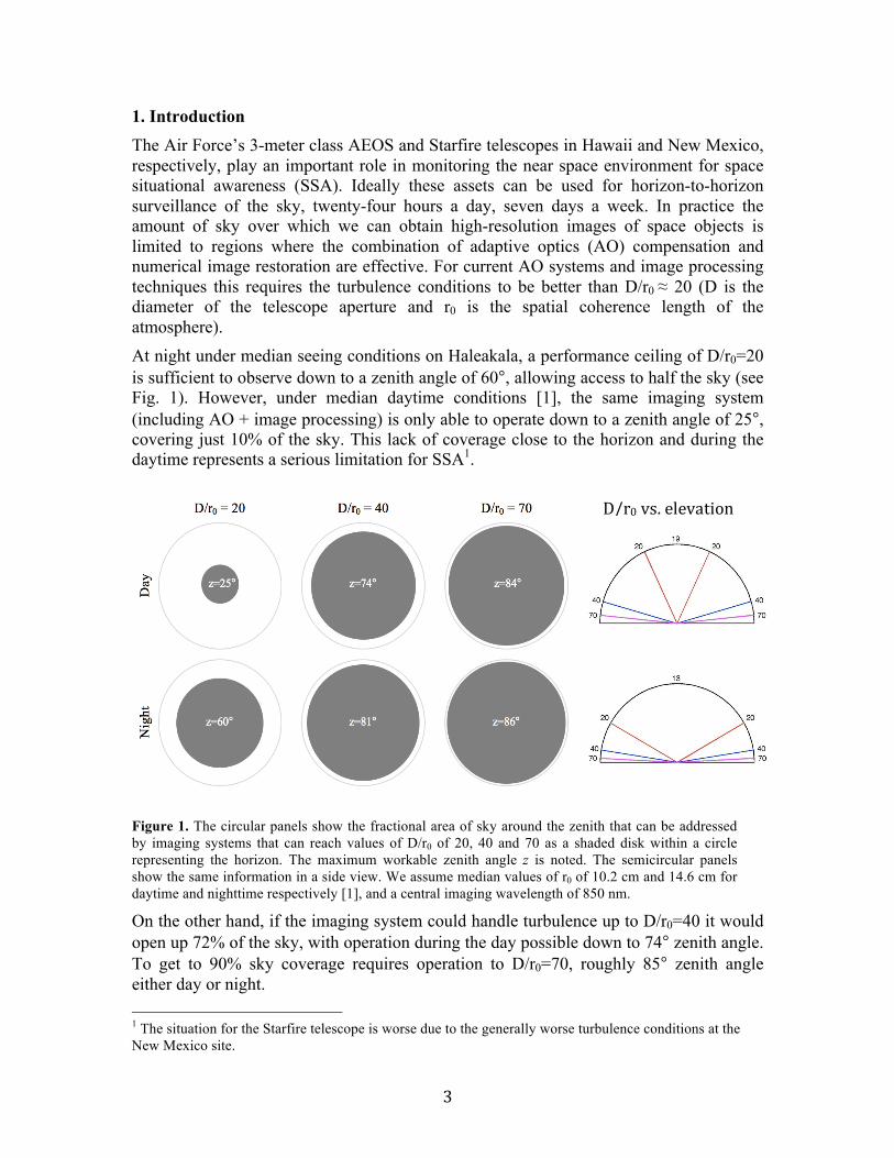
1. Introduction The Air Force’s 3-meter class AEOS and Starfire telescopes in Hawaii and New Mexico, respectively, play an important role in monitoring the near space environment for space situational awareness (SSA). Ideally these assets can be used for horizon-to-horizon surveillance of the sky, twenty-four hours a day, seven days a week. In practice the amount of sky over which we can obtain high-resolution images of space objects is limited to regions where the combination of adaptive optics (AO) compensation and numerical image restoration are effective. For current AO systems and image processing techniques this requires the turbulence conditions to be better than D/r0 ≈ 20 (D is the diameter of the telescope aperture and r0 is the spatial coherence length of the atmosphere). At night under median seeing conditions on Haleakala, a performance ceiling of D/r0=20 is sufficient to observe down to a zenith angle of 60°, allowing access to half the sky (see Fig. 1). However, under median daytime conditions [1], the same imaging system (including AO + image processing) is only able to operate down to a zenith angle of 25°, covering just 10% of the sky. This lack of coverage close to the horizon and during the daytime represents a serious limitation for SSA1.

Figure 1. The circular panels show the fractional area of sky around the zenith that can be addressed by imaging systems that can reach values of D/r0 of 20, 40 and 70 as a shaded disk within a circle representing the horizon. The maximum workable zenith angle z is noted. The semicircular panels show the same information in a side view. We assume median values of r0 of 10.2 cm and 14.6 cm for daytime and nighttime respectively [1], and a central imaging wavelength of 850 nm.

On the other hand, if the imaging system could handle turbulence up to D/r0=40 it would open up 72% of the sky, with operation during the day possible down to 74° zenith angle. To get to 90% sky coverage requires operation to D/r0=70, roughly 85° zenith angle either day or night.                                                                                                                1 The situation for the Starfire telescope is worse due to the generally worse turbulence conditions at the New Mexico site.

D/r0  vs.  elevation  angle  

  4  

The focus of our research is to advance the surveillance capabilities of the Air Force’s large aperture telescopes by developing methods that will enable high-resolution imagery to be obtained through turbulence conditions with D/r0 >> 20, thus dramatically increasing both the area of the sky and the amount of time we can monitor the near space environment. 1.1 Correction of wave front aberrations caused by atmospheric turbulence

To obtain the full resolution performance of an imaging system when viewing through the Earth’s atmosphere requires careful mitigation of the turbulence-induced aberration in the observed wave front. This is typically achieved through the use of adaptive optics followed by post-detection numerical processing. The latter is required to correct for residual wave front distortions that were not compensated by the AO system. Because the details of the remaining image blur are often not well known, the processing technique of choice is multi-frame blind deconvolution (MFBD, [2,3]). The maximum improvement in resolution achieved by an AO system, as measured by the Strehl ratio (the ratio of the maximum intensity in a point source image to that in its theoretical diffraction-limited image), occurs for D/r0 = 2.3 (qN)½ [4]. Here q is a measure of the AO system’s compensation efficiency and N is the number of actuators in the system. When D/r0 increases above ~2.3 (qN)½ the performance of the AO system begins to deteriorate. For an AO system equipped with a large-format deformable mirror (N~1,000; q~0.05 [4]) the deterioration starts at D/r0~16.

The performance of MFBD also depends on the strength of the turbulence and is best at low levels of turbulence (small D/r0 values). This is because the algorithm is susceptible to entrapment in local minima during the iterative optimization process [5] and the number of local minima rapidly increases as the number of speckles in the atmospheric point spread function (Nspeckles~ (D/r0)2) increases. From our experience MFBD loses effectiveness for D/r0>20.

The overall performance of the AO-numerical processing combination is such that imagery with diffraction-limited resolution can be produced for observations acquired through turbulence strengths of up to D/r0 ≈ 15, after this the resolution starts to degrade. There are two ways to extend the diffraction-limited performance beyond this. The first is to improve the performance of the AO compensation by increasing N and/or q. The second is to improve the performance of the restoration process.

Unfortunately, a large improvement in AO performance is hindered by the practicality that q tends to decrease as N increases [4]. There are also signal-to-noise considerations in the wave front sensing component of AO when increasing the density of the micro-lens array in the wave front sensor (WFS).

This leaves the second approach. Here we need to develop techniques to avoid local minima during the restoration process and methods to improve our estimation of the atmospheric wave front. As we will see, these both require, in part, that we improve the synergy between the image acquisition and processing steps: this is in stark contrast to the current approach where the two steps are essentially independent of each other.

  5  

2. Incorporating wave front sensor data in the restoration process A first step toward improving the performance of the restoration process is to incorporate wave front sensor (WFS) data that were taken simultaneously with the image data, in to the restoration process [6]. These additional data, that contain information on the residual wave front error, provide a strong physical constraint on the parameter values for the wave front phases in the restoration. However, the leverage provided by this constraint quickly decreases once r0 falls below the WFS sampling distance. This is a potentially serious limitation for observing through strong turbulence as the high-spatial frequencies of the wave-front phase become increasingly influential on the morphology of the point spread function (PSF) as r0 decreases, and thus ever more important to estimate (see Fig. 2). Fortunately, there is some salvation available if we model the temporal correlations in the atmospheric wave front.

Figure 2. The top row shows a Kolmogorov phase screen with different scaling and filtering. The screen in the top left represents D/r0 ~ 3 conditions and the filtered version of this screen (convolved with a Gaussian function with FWHM ~3 pixels) is shown next to it on the right. The next panel (top, center, right) is the D/r0~3 phase screen scaled to represent D/r0~ 40 conditions. The far right panel is the D/r0~40 phase screen filtered in the same way as for the D/r0~3 data. The bottom row shows the corresponding PSFs for the phase screens that are above. It is clear that the sensitivity of the morphology of the PSF to the high-spatial frequencies of the wave front phase dramatically increases as the level of turbulence increases.

  6  

2.1 Modeling the atmospheric turbulence using the Taylor frozen flow hypothesis The Taylor frozen flow hypothesis (FFH) assumes that, over short time scales, atmospheric turbulence can be modeled by a series of independent static layers moving across the telescope aperture, each layer moving with the prevailing wind at the altitude of the layer. The relevant time scale for a single layer is given by the time taken for the wind to carry the (frozen) turbulence a distance r0, i.e., τ0 ~ r0/v, where v is the wind velocity. This “coherence time” therefore varies according to site and atmospheric turbulence conditions. For multiple layers v is replaced with <v>/0.3, where <v> is the mean velocity over the layers weighted by the CN

2 profiles [7]. The validity of the FFH has been verified by Schöck & Spiller [8] for observations at the Starfire Optical Range in New Mexico. They observed, using a cross-correlation analysis of wave-front sensor (WFS) data taken at 0.74 µm with low-level wind velocities of ~ 4 m/s and turbulence with r0≈4cm, that use of the FFH is accurate for time scales of ~20 ms or less: the accuracy degrading with increasing time such that by ~100 ms only 50% of the temporal evolution can be described by the FFH. Figure 3 shows that for the period the turbulence can be described by a frozen flow, a time series of wave front phase gradient data from the Shack-Hartmann WFS contains information on spatial scales finer than the separation between detectors in the WFS [20, 24].

To use the FFH requires that we know the wind velocities of all significant layers of turbulence in the atmosphere. These are computed from an autocorrelation of the WFS measurements, which are captured at a cadence that substantially exceeds the Greenwood frequency and therefore capture the effects of frame-to-frame coherence in the wave front. The measured wave-front slopes are stacked into a data cube and the 3D spatio-temporal autocorrelation of the cube is calculated. Consider the effect of a wave front characterized by a single frozen layer moving across the pupil. The strongest signal will

Frame 1

Frame 2

Frame 3

Frame 4

Frame 5 Frame 6

Composite grid

Figure 3. The images in the top row show how a Shack-Hartmann array samples the underlying frozen phase screen as it moves across the telescope aperture. The image on the bottom shows the effective sampling of the phase by the time series data in the top row.

  7  

occur at the center of the autocorrelation cube, at zero spatial and temporal lags. But as time progresses, and the wave front advances across the aperture, the strongest correlation signal will be seen at a spatial lag equal to the elapsed time multiplied by the wind vector. The signature of a frozen layer is thus a line of strong signal projecting from the origin of the autocorrelation cube whose direction corresponds to the direction and speed of the corresponding wind, illustrated in Figure 4. The strength of the correlation signal is directly related to the strength of turbulence in the layer, and the rate of decay with temporal lag indicates the degree to which the layer is not in fact well represented as a frozen flow.

Under the FFH we can model the total wave-front phase distortions in the pupil,  Φ(x,t), as   Φ(x,t+Δt) = Σi αi(x-­‐viΔt,t),         (1)    

where αi  =  φi  ⊗  ηi are the phase delays caused by layer i at time t, vi is the velocity of this layer,  φ are the model parameters,  η  is a Gaussian kernel that enforces spatial correlation in the phases, ⊗  denotes convolution and  Δt   is the time between WFS frames. We can reconstruct the phase by finding the  values  of  φ  that  minimize the cost function    

εwfs=  Σk Σx  M{|∇xΦ  –  Sx|2  +  |∇yΦ  –  Sy|2}.       (2)    

Here Sx , and Sy are the measured x and y gradients of the phase for time index k, ∇ is the gradient operator, and M is a binary mask representing the location of each sub-aperture in the Shack-Hartmann sensor. Figure 5 shows the improvement in the reconstructed phase when using this approach, which accounts for the temporal correlations in the wave front, over that where the temporal correlations in the wave front are ignored.

This higher-fidelity wave front estimate can be leveraged in the numerical processing of the corresponding focal plane imagery.  2.2 Deconvolution from Wave Front Sensing (DWFS)

DFWS is an image-reconstruction technique that is normally thought of as providing a low-cost, post-detection, alternative to adaptive optics for compensating for the image degradation due to atmospheric turbulence [9,10]. However, it is also a powerful tool for use with short-exposure AO-compensated data. DWFS requires the simultaneous recording of short-exposure, focal plane, images and WFS data.

Figure 4. Consecutive time-lag slices from the 3D autocorrelation of real Shack-Hartmann WFS data obtained at the 3.6 AEOS telescope on Maui. Two frozen layers, noted by the arrows in frame 4, are detected as spots of high signal projecting from the origin.

Time lag

  8  

Figure 5. The left panel shows the reconstructed phase based on a single frame of Shack-Hartmann WFS data. The right panel shows the reconstruction based on a series of Shack-Hartmann WFS data and the use of the FFH. The improvement in the estimation of the high-spatial frequencies of the wave front is clear.

Traditionally, the WFS measurements are used to estimate the point-spread functions for the observations. These PSFs are then used with the ensemble of short-exposure images to obtain an estimate of the object intensity distribution through deconvolution. This approach for the object estimation, however, does not take into account any errors in the wave-front phase reconstruction process. An alternative approach, which overcomes this limitation, is to perform a joint estimation of the object and the wave fronts [6,11].

We adopt the isoplanatic, incoherent, imaging model and model the observed focal plane data, g(x), as a convolution between the object, f(x), and the atmospheric point-spread function h(x). That is,

𝑔  (x) = (𝑓  ⊗ ℎ)x . (3) Here the “hat” symbol denotes an estimated quantity (as opposed to a measured quantity). We model the point-spread functions and object using ℎk(x) = (1/J) Σj

|FFT-1{Pkj(u) exp(iΦkj(u))}|2 (4) and 𝑓(x) ≡ FFT-1{Σk Gk(u)𝐻k

*(u)/[Σk 𝐻k(u)⋅]𝐻k*(u) + γ]}, (5)

respectively. Here P(u) are the wave-front amplitudes in the pupil (assumed to be unity), FFT-1{} is the inverse Fourier transform operator, g is a regularization parameter, * denotes complex conjugate, h(x)⇔H(u), g(x)⇔G(u) are Fourier transform pairs, and γ is a regularization constant. The summation over j represents the scenario where the WFS data are accumulated at a higher frame rate than the focal plane data (i.e. there are J WFS frames for each focal plane frame). We note that without the FFH, Eqn. (1) is replaced by Φ(x,t)=α(x,t) and the phases at different times are treated as independent realizations of the atmosphere. We estimate the values of φ by minimizing the error metric

εTotal = ε + Σj εjwfs, (6)

  9  

using a partial conjugate gradient approach [11], where ε = Σk Σx |𝑔k(x) – 𝑔k(x)|2 (7) and 𝑔k(x) are the observed focal plane data. We note that minimization using just the error metric in Eqn. (7) constitutes traditional MFBD: the addition of the WFS metric changes the situation to “myopic” deconvolution [11]. Small deviations from the frozen flow behavior, for example due to turbulent boiling, can be accounted for in practice by performing a second run of the DFWS algorithm. In this run each frame is treated as an independent realization of the atmosphere: this allows for the necessary small updates to the phase estimates. We also note that data sets that cover periods much longer than the atmospheric coherence time can be modeled using a series of overlapping frozen flow screens.  Lastly, use of the FFM has the added benefit of requiring the estimation of significantly fewer parameters than a description where there is no frozen flow behavior because successive frames of data see substantially the same wave front. This contributes to reducing the number of local minima in the optimization. 2.3 Simulations We tested our DFWS algorithm using numerical simulations of astronomical observations made with the 3.6m AEOS telescope on Mount Haleakala and zero read noise detectors. Site surveys have shown that the atmosphere above Mount Haleakala can be reasonably well approximated by two turbulent layers: one at ground level with a velocity of ~5 m/s, the other at a height of 11km with a velocity of ~29 m/s [12]. The details of the simulations are given in the appendix. We have simulated observations of the Hubble Space Telescope (mv=2.3) taken using a 10 arcsec x 10 arcsec field-of-view (FOV) without AO compensation. With this FOV and the site characteristics noted above, the diameter of the meta-pupil at 11 km, relative to the telescope aperture – given by (1+ 2θzi/D –zi/R), where θ is the FOV angle, zi is the height of the ith turbulent layer and R is the height of the target (569 km) - is only 12% larger than the telescope aperture. In addition, the relative footprint in this meta-pupil of each point in the FOV - given by (1 – zi/R) - is only 2% smaller than the telescope aperture. That is, anisoplanatic effects will be small and we can still obtain a reasonable modeling of the phases using Eqn. (1) without having to resort to geometric ray tracing or Fresnel propagation methods. 2.4 Results Two experiments were performed for simulated observations acquired through strong turbulence conditions (D/r0~50). In the first experiment, the FFH is used to model the wave-front phases in two layers. In the second, temporal correlations between frames are

  10  

ignored and the wave-front phase in each frame is treated as an independent realization of the atmosphere. In both cases, spatial correlations are enforced in the estimated phases using η=4 pixels (i.e. the FWHM of the Gaussian smoothing kernel ~ sub-aperture spacing), and the minimization is stopped when the estimated phases show no evidence of further change. The initial estimates for the wave front phases in both cases, is zero. Figure 6 shows that use of the FFH provides a restored image with a spatial resolution that is far superior to the restoration without inclusion of temporal correlations in the wave-front phase. In the latter the restoration quality is so poor that no meaningful information can be obtained on the target object.

Figure 6. Left: Diffraction-limited image of the truth object (Hubble Space Telescope). Middle Left: Image after convolution of truth object with truth PSF and addition of photon noise. Middle Right: Restored image from 40 frames (80 msec) of focal plane and WFS data when using the FFH. Right: Restored image without use of the FFH. All images are shown with linear scaling.

We also looked at a case of extreme turbulence (D/r0~100). Even here, the additional high-frequency information on the wave front that can be recovered using the FFH is sufficient to extract some information on the target from data that would normally be discarded (see Fig. 7).

Figure 7. Left: Simulated image of the Hubble Space Telescope observed through strong turbulence (D/r0~100). The simulations ignored variations in the wave front amplitudes, an approximation that is not valid for observations at low elevation angles. Right: The restored image produced using the technique of deconvolution from wave-front sensing and the wave fronts estimated using simultaneously acquired Shack-Hartmann wave-front sensor data and known information on the temporal behavior of the atmospheric turbulence.

  11  

2.5 Discussion

The FFH allows for an effective sub-sampling of the wave-front phase that facilitates the reconstruction of the high-spatial frequencies in the phase that are not sampled by the sub-apertures in the WFS. This property allows us to extend the range of imaging conditions over which DFWS can be used to obtain high-quality restorations: basically to conditions where r0 is less than the sub-aperture spacing (e.g., shorter wavelengths, strong turbulence), a regime where AO compensation loses its effectiveness.

3. Avoiding entrapment in local minima during the restoration process   As noted in §1.1, MFBD algorithms are susceptible to entrapment in local minima during the iterative optimization process [5] thus producing a sub-optimal restoration. A common gambit to mitigate this problem is to enforce known physical and mathematical constraints onto the solution (e.g., positivity of the object brightness). Unfortunately, this only works for imagery obtained through relatively benign turbulence. As the complexity of the PSFs increases with increasing turbulence, the number of local minima also increases and entrapment still occurs despite the additional constraints. Some extension of the turbulence strength at which entrapment becomes inevitable can be obtained by using high-quality initial estimates for the object and PSFs to position the algorithm well in parameter hyperspace (i.e. close to the global minimum). However, for imaging scenarios where WFS data are not available, high-quality initial object and PSF estimates are generally hard to come by. The solution to this problem lies in the fact that MFBD typically performs well at low turbulence.

3.1 Aperture diversity and MFBD In our experience MFBD algorithms struggle when D/r0>20. To tackle restorations in this regime, we seek a strategy in which we first solve a problem with small D/r0 and then use the result to seed a problem with more severe aberration. By successively applying this approach to problems of larger and larger D/r0, we may bootstrap ourselves through the parameter hyperspace avoiding local minima along the way. In this way, we can hope to compute a successful restoration at the diffraction-limited resolution of the full aperture even for strong turbulence conditions. This hierarchical approach is similar to objective function smoothing techniques used in numerical optimization [13] to avoid local minima, but instead of explicitly modifying the objective function by, for example, Gaussian smoothing, the smoothing is done implicitly with smaller D/r0 values. What is needed is a way to acquire the image data such that the restoration can be carried out as a number of separate MFBD problems spanning a range of D/r0 values from very small to that for the full aperture. A straightforward way to do this is to use aperture diversity imaging [14] where the diversity is in the aperture size. The simplest implementation of the strategy is to record images of the same object simultaneously with a number of telescopes of different aperture size. If the smallest is arranged to have D/r0<10, a straightforward MFBD analysis will yield a good estimate of the object at low spatial frequencies (that is, the

  12  

object estimate is of low resolution) that may be used to seed restorations from the next largest aperture, and so on. The PSFs of the different telescopes will share nothing in common, even if the image sequences are carefully synchronized, because the atmospheric aberrations will be uncorrelated. Nevertheless, we can still apply a strong constraint on the PSFs for the larger telescopes. In the ratio of the spectra of observations from two telescopes, the common object spectrum cancels out, leaving the ratio of the PSF spectra [15]. With the PSF estimates for the smaller telescope derived from MFBD, a good starting estimate may also be found for the PSFs from the larger telescope.

A more powerful approach to aperture diversity is to partition a single large telescope aperture into annuli and to form separate images through each annulus [16]. The outer diameter of the smallest annulus is set so that D/r0 is low; again, MFBD of the data provides a high fidelity, low-resolution estimate of the object. Higher resolution estimates are then successively calculated as before, by introducing data from the larger annuli. Better performance from this arrangement than from the physically separated telescopes can be obtained, as we describe below, by adopting a restoration algorithm that estimates the wave-front amplitude and phase in the pupil as well as the object, and exploits the characteristic of atmospheric turbulence that over short time scales it is well described by the Taylor frozen flow model.

3.1.1 Wave front sensing using multi-aperture phase retrieval In §2 we showed how modeling the temporal correlations in the wave front, using the frozen flow approximation, facilitated increased sampling of the wave front over that afforded by the wave front sensor sampling. This increased sampling is in the direction of the wind vectors for the different turbulent layers. However, to provide the best possible estimate of the wave front it would be best to have increased sampling in all directions. This can be achieved by operating the Shack-Hartmann WFS in the same way as is used in solar adaptive optics [23].

The Shack-Hartmann (SH) WFS divides the telescope aperture into a set of contiguous square sub-apertures. It can therefore be regarded as another instance of aperture diversity. But we can extend the information recoverable from this arrangement by making a critically sampled image of the full field through each sub-aperture, rather than the hugely under-sampled (point-source like) images typically made by a SH WFS. We will refer to the former as an imaging SH WFS.

The sub-apertures in an imaging SH WFS are sized to yield D/r0 values less than 10 so that MFBD of the images from a sub-aperture can provide a good solution [17,18]. Now, the data from a single sub-aperture provide information on both the wave front in that sub-aperture (beyond simple tip-tilt) and the lowest spatial frequencies of the object. The reconstructed wave fronts from all the sub-apertures taken together provide an estimate of the wave front across the full telescope’s pupil. This estimate will have the necessary high-spatial frequency information for the restoration of images acquired at high turbulence strengths, with the information now no longer constrained to lie along the frozen flow wind directions. We still take advantage of the frozen flow behavior of the atmosphere, which now provides an extra benefit beyond the recovery of high-spatial frequency wave-front information. Critically, it allows us to estimate the wave-front phases unambiguously. As

  13  

is well known, the wave front cannot be uniquely determined from a single image because an overall sign change in even modes of the aberration leaves the PSF unchanged. Typically, an approach such as phase diversity is required to establish the sign. But the propagation of the phase across the pupil between successive images in increments of a fraction of the sub-aperture size effectively introduces the needed diversity, and the wave-front solution becomes unique.

3.1.2 Combining approaches The approach we have adopted for image restoration at high D/r0 combines the bootstrap approach to the restoration process, starting with low D/r0 data and progressively adding in larger D/r0 data, with the multi-aperture phase retrieval technique for measuring the high-spatial frequencies of the wave front. The optical implementation is sketched in Figure 8. Here the light beam is split into two channels, each of which is relayed to a pupil where the light is segmented: one channel with a grid of small rectangular-like sub-apertures, the other in concentric annuli. The light from each sub-aperture is imaged onto separate detectors. Only the images from the largest annular sub-aperture contain spatial frequencies out to the diffraction limit of the telescope. All the others yield imagery with lower spatial frequency content. We therefore refer to the channel with the annular sub-apertures as the “high-resolution” channel, and the other channel as the “low-resolution” channel. In summary, in this aperture diverse setup the input light that would normally be collected by a single aperture is now shared over a large number of apertures designed to

yield image data with a range of D/r0 values.

3.2 Simulated data To test our proposed aperture diversity technique we use numerical simulations of observations of the Hubble Space Telescope (HST) taken through atmospheric turbulence with r0~9 cm with a 3.6 m telescope. At D/r0=40, the simulated data are therefore well beyond the regime of turbulence strength that classic MFBD techniques can address. We note that r0~9 cm is commensurate with the mean daytime seeing at Mount Haleakala for an observing wavelength of 850 nm [19]. The data consist of images from 24 apertures,

Figure 8. This cartoon shows the proposed aperture diversity instrument. The focal plane array associated with the micro-lens array constitutes the “low-resolution” channel; the focal plane arrays associated with the annular sub-apertures constitute the “high resolution” channel.

  14  

each of size ~0.6 m in the low-resolution channel and 2 annular apertures with diameters of 1.6 m and 3.6 m in the high-resolution channel. The target is assumed to have a brightness of mv=+2, which corresponds to 1.1×107 photons/image for the full 3.6 m aperture for a 2 ms integration [20]. Half the light is sent into each channel, which results in approximately 40% of all the input light going to the large annulus. Figure 9 shows

example images for the different apertures. We use a two-layer, frozen flow description of the atmosphere and a Kolmogorov model to generate the PSFs for the different apertures. The wind velocity vectors are commensurate with values observed at Mt Haleakala (~5 m/s for the lower layer and ~ 30 m/s for the upper layer [12]). The resulting PSFs are convolved with a numerical model of the HST to provide noise-free models of the observed images. Poisson noise is then added to these images to simulate the observed data. Since it is not fundamental, we do not include read noise from the detectors, assuming that devices such as noiseless EMCCDs will be used. We generated a time series of 16 simulated speckle observations, each comprising 26 channels, with exposure times less than the coherence time of the atmosphere, as would be made with the proposed aperture diversity system. From the same atmospheric realizations we also generated simulated images as would be made using a single 3.6 m telescope.

3.3 Multi-aperture MFBD algorithm We use a modified version of the DWFS algorithm described in §2.2.

Figure 9. Top row: Sample data frames from numerical simulations of observations of the Hubble Space Telescope taken with different apertures, shown in the bottom row, through atmospheric turbulence with r0~9 cm. Left to right: 3.6 m full aperture (with 0.75 m central obscuration), 3.6 m diameter annulus (1.6 m inner diameter), 1.6 m annulus (0.75 m inner diameter), a central low-resolution sub-aperture (~0.6 m size). The data frames are displayed on linear scales between each image’s minimum and maximum values. The total number of photons in the 26 images from the multi-aperture data set at each time is equal to the number of photons in the single image from the 3.6 m filled aperture.

  15  

The first modification is that we describe the object intensity distribution using the parameterization f (x) =ψ 2 (x) . The real function ψ(x) is described using a 2-D pixel basis set. The second modification is that the data model for each channel, denoted by l, is given by

(8)

where the scalar al accounts for the different photon fluxes in each channel due to the different sizes of the apertures. The corresponding update to the convolution error metric is

ε = gl,k (x)− gl,k (x)x∑k∑2

l∑ (9)

For an aperture diverse (AD) observation the number of imaging channels is equal to the number of sub-apertures in the low-resolution channel plus the number of annular partitions of the full aperture. For traditional single aperture observations the number of imaging channels is equal to 1. The set of model parameters now includes and . For multi-telescope data, where the frozen flow approximation cannot be used to connect the separate apertures, we leverage the information contained in the observed spectral ratios. In the case of noise-free data, the spectral ratio (the ratio of the Fourier spectra of two data frames ) is independent of the object spectrum (assuming the object is the same in each frame [15]). That is, (10)

for where is the optical transfer function (OTF), are the additive noise components for the and frames and the PSFs are assumed to be spatially invariant and incoherent. If the OTF is well known for one of the frames, then by using the observed spectral ratios we immediately have good estimates of the OTFs of the other data frames. In the case of spectral ratios for data obtained with two-channels with different cut-off frequencies, the spectral ratios are valid over the common frequency range. This constraint on the PSFs is enforced using the consistency metric

εSR = M l !l ,k !k (u) χ l !l ,k !k (u)2

G j (u)2

j∑u∑k , !k∑l , !l∑ (11)

where

(12)

Here is a binary mask equal to 1 at a given spatial frequency when the SNR for the and frames in the and channels is greater than some chosen threshold, which we arbitrarily set to 100.

gl,k (x) = αl f!x∑ (x− !x )hl,k ( !x )

ψ(x) Φ(u)

Gk (u) / Gk ' (u) F(u)

Gk (u) / Gk ' (u) = F(u)Hk (u) + Nk (u)!" #$ / F(u)Hk ' (u) + Nk ' (u)!" #$ → Hk (u) / Hk ' (u)

( ) ( ) 0k kN u N uʹ′= = ˆ ( )kH u ( ), ( )k kN u N uʹ′thk thkʹ′

χ l !l ,k !k =G !l , !k (u)H l ,k (u)−Gl ,k (u)H !l , !k (u)

G !l , !k (u)G !l ,k (u).

M l !l ,k !k (u) =M l ,k (u)M !l , !k (u)

k k ʹ′ l lʹ′

  16  

At each step in the bootstrap process where the next higher resolution data are introduced into the MFBD problem, the low-resolution wave-front phases are fixed and the consistency metric used to update the wave fronts on the higher resolution channel. Once the value of the metric has plateaued, the minimization is stopped, and restarted as an MFBD problem using the previous lower resolution object and PSF estimates with the new wave-front estimates in the higher resolution channel. This update of the high-resolution wave fronts encodes the position of the target, such that the lower resolution object can be used as a start for this new MFBD problem. 3.4 Results

The effectiveness of the bootstrap process is highlighted in Figure 10, which shows the error in the object estimate as a function of spatial frequency. The root-mean-square error (RMSE) is the root-mean-square difference between the true and estimated object power spectra, azimuthally averaged in the Fourier plane, over 20 random trials. Figure 10a shows the error after standard MFBD processing of speckle data sets collected with telescopes of 1m, 1.6m and 3.6m diameter. For this experiment, the seeing was characterized by r0 = 15 cm. It is noteworthy that the best estimates of the lowest spatial frequencies are obtained from the smallest aperture even though it sees nearly ten times less light than the largest aperture. Figure 10b shows the result of processing the three data sets combined. If all three are processed simultaneously, then the result is very similar to the result for the 3.6 m aperture alone (Figure 10a): the addition of the data from the smaller telescopes does not help. In contrast, if the data sets are processed in series from smallest to largest aperture, following the bootstrap prescription, the RMSE is substantially reduced at all spatial frequencies. This highlights the fact that it is the local minimum problem that provides the main limitation to MFBD performance in poor seeing.

0 0.2 0.4 0.6 0.8 10

1

2

3

4

5

6

7

8

9

10

Fraction of 3.6m Diffraction Limited cut−off

RM

SE

0 0.2 0.4 0.6 0.8 10

1

2

3

4

5

6

7

8

9

10

Fraction of 3.6m Diffraction Limited cut−off

RM

SE

a   b  

Figure 10. (a) The variation of the RMSE vs. spatial frequency based on a Monte Carlo of 20 trials of 6-frame blind restorations for simulated data of a target of brightness mv=+2 as would be acquired with telescopes of 1 m (blue line), 1.6 m (magenta line) and 3.6 m (green line) observing through the same atmosphere (r0~15 cm). The lower the RMSE value, the better the quality of the restoration. (b) The RMSE of images recovered using the combined data from all three telescopes. The green line represents the simultaneous restoration of the combined data. The black line represents a bootstrap approach that starts with the smallest aperture data to achieve a good low-spatial frequency estimate, and then systematically updates the estimate through the additions of data from the larger apertures.

  17  

The results of processing the simulated aperture diverse and conventional speckle data described in §3.2, using our modified MFBD algorithm, are shown in Figure 11. The gain provided by using aperture diverse speckle observations over traditional speckle observations with a 3.6 m telescope is clear; the former provides an image that exhibits good high-spatial frequency information, whereas the latter provides an image with severely limited resolution and a high level of artifacts.

Figure 11. Simulated images of HST. (a) Diffraction-limited image for a filled aperture 3.6 m telescope; (b) restoration of a data set from a filled aperture 3.6 m telescope only; (c) restoration of aperture diverse images from our proposed instrument. All images are displayed on the same linear scale.

Three effects contribute to the improvement in the restoration with the aperture diversity arrangement compared to the single 3.6 m aperture. In the first place, by dividing the pupil into sub-apertures, the data are readily analyzed to estimate physical parameters that cannot be extracted from the filled aperture data; in particular, the mean slope of the wave front across each sub-aperture and the wind vectors associated with strong layers of turbulence. This information is used to solve a least squares problem to estimate the wave-front tilt across the full pupil for each layer. Knowing the global layer tilts, and by applying a Gaussian convolution kernel (with standard deviation of 1 pixel) to the wave front, we enforce continuity of the phase across the boundaries of the sub-apertures. Secondly, with knowledge of the wind vectors, we apply the FFH to model the flow of atmospheric phase errors over the contiguous apertures of both channels. This allows us to reduce the number of variables that must be solved in the problem by more than a factor of five. The variables may be viewed as axes of a Hilbert space within which an error hyper-surface is defined, whose global minimum we seek. The FFH enormously reduces the dimensionality of the search, and thereby the number of local minima into which the solution can irretrievably fall. The importance of this reduction is easily overlooked: it is analogous to reducing a 5-dimensional search to a 1-dimensional search.

Finally, by initially working only with the low-resolution sub-apertures, the search is restricted to a hyper-plane within the Hilbert space, further reducing the dimensionality of the problem. Furthermore, since these apertures see phase errors with only low D/r0 values, we choose the hyper-plane in such a way that the number of local minima is comparatively small. Only after the best point in the hyper-plane has been found do we then successively introduce the remaining regions of the full space, once again minimizing the dimensionality to be searched at any one time.

a   b   c  

  18  

3.5 Separation of wave-front layers

In addition to providing a high-resolution image of the target, the aperture diversity approach also yields high-fidelity wave-front estimates with minimal artifacts.

Furthermore, the atmospheric turbulence layers are individually well estimated: the FFH applied to the annular partitioned data enables the phase contributions from the layers to be disentangled. Figure 12 shows an example result from the two-layer atmospheric model, where the height of the lower layer was set to zero, and the upper layer was set at 5200 m to match the observed median value of θ0, the isoplanatic angle, at Mt. Haleakala [19]. This behavior suggests that the aperture diversity approach may be used to restore images with fields of view substantially larger than the isoplanatic angle. With knowledge of individual atmospheric layers and their ranges, PSFs may be constructed along widely separated lines of sight. The effectiveness of the approach is illustrated in Figure 13. Here

Layer  1  

Layer  2  

Truth   Estimate  

Figure 12. Wave-front phase after removal of global tip/tilt: layer 1 (top row) layer 2 (bottom row). The true phases are in the left column; the estimated phases are in the right column. The images in each row are displayed on the same linear scale.

Figure 13. Strehl ratio achieved with wave-front compensation using the estimates of Fig. 5. Upper curve: correction calculated from the two layer estimates separately along the line of sight. Lower curve: correction assumed to be the on-axis sum of the two estimated layers.

  19  

we have calculated the Strehl ratio for PSFs computed using two different methods of wave-front correction. Naïve correction using the integrated wave-front error on axis shows the classic anisoplanatic behavior, with reasonable on-axis Strehl ratio of 0.81 that drops off rapidly with field angle. By 2θ0, or about 6 arcsec, the Strehl ratio has dropped to a negligible value. By contrast, when the individual layer estimates are used to calculate a correction along a chosen line of sight, the performance is enormously improved out to field angles an order of magnitude larger than θ0. The proposed aperture diversity approach is instrumentally more complex than the phase diversity approach used by Thelan et al. [21], however, it may provide stronger leverage on the separation of the turbulent layers thus allowing for use in stronger turbulence conditions: further investigation is needed. We note that in both the phase diverse and aperture diverse cases we will have to solve the anisoplanatic restoration problem. 3.6 Optical super-resolution

In addition to providing an estimate of the observed wave fronts, the first pass through the bootstrap process, which uses only the low-resolution channel data, also provides a low spatial-frequency estimate of the target. Interestingly, we find that the recovered image is well estimated out to a spatial frequency cut-off that exceeds the diffraction limit of the sub-apertures. The level of this optical super-resolution, illustrated in Figure 14, is quite dramatic.

Information theory has shown that optical super-resolution is possible because the number of degrees-of-freedom of an optical signal that an imaging system can transmit is constant. By having some a priori knowledge about the signal therefore, we can encode-decode additional spatial frequency information onto the redundant degrees of freedom to increase spatial bandwidth while maintaining the total number of degrees of freedom [22]. One example of suitable a priori information, which is pertinent to the study here, is when the signal can be considered stationary with time. Here optical super-resolution is obtained through temporal multiplexing by encoding the image scene while forming a time series of low-resolution images, and then using the knowledge of the encoding to form a high-resolution image afterwards. We speculate that the “frozen flow” behavior of the atmosphere is providing an analogous spatial-temporal encoding in our atmospherically distorted imagery and that the FFM in the restoration process provides the decoding. This remains to be verified.

Figure 14. Left: The mean diffraction-limited image for the apertures of the low-resolution channel. Right: The restored image from this channel alone using the frozen flow model for the atmosphere.

  20  

3.7 Discussion Using numerical simulations we have shown that the proposed aperture diversity approach is capable of separating the object signal from the atmospheric blur signal for imagery acquired through strong atmospheric turbulence (D/r0=40). By dividing the input signal across a number of different size apertures we dramatically improve the synergy between the data acquisition and processing steps. In particular, the resulting restoration algorithm becomes robust against entrapment in local minima, the bane of blind restoration algorithms. A potentially valuable side benefit of the approach is that it enables physically meaningful separation of the phases in different layers of the atmosphere. This opens up the possibility to restore images across a wide anisoplanatic field-of-view. As a final remark, we note that we have focused on the challenge of imaging through strong atmospheric turbulence. However, the techniques we have developed are equally suited to high dynamic range imaging at lower turbulence strengths. Here the emphasis is on accurately modeling the PSF structure out to large radial distances to capture the low amplitude speckle structure. This is essential to obtain restorations with high-dynamic range, and requires faithful estimation of the wave-front phases. Without this, the restored image will always have a faint “fog” which may mask any faint objects present in the image.

 3.8 Compact multi-frame blind deconvolution (CMFBD) A second spectral ratio-based prior term, that enforces positivity on the estimates for the PSFs, is given by

𝜀!"! =2

1

1

( )ˆ( ) ( )( )

K Jj

jk kk j k x ve k

G uF M u H u

G u−

= > −

⎧ ⎫⎨ ⎬⎩ ⎭

∑∑∑ (13)

where

F −1 A{ } denotes the inverse Fourier transform of A ,

M j ,k (u) is a similar mask to

Mkk ' (u) and the summation over x is only over pixels with negative values. This prior has application only in the case when the user wants to perform “compact” MFBD (CMFBD), where the object and PSFs are explicitly modeled for a subset of the data frames ( K “control” frames) but all the data frames ( N ) are used to leverage the restoration [15]. Such a case can occur when N is very large and the number of variables required to model all the data is impractical due the large dimensionality of the parameter hyperspace. This leads to inevitable entrapment in local minima during the optimization. In CMFBD the J ( = N − K ) “non-control” frames still provide leverage on the restoration through this prior that demands that the PSFs for the non-control frames be positive. These PFSs are estimated via spectral ratios, and the PSF estimates for the control frames are modeled as a band-limited positive function. This prior provides a “hard” constraint for an object whose Fourier spectrum extends over the entire spatial frequency range sampled by the atmospheric OTFs (e.g. a star). But this is only a “soft” constraint for an object with a more compact Fourier spectrum that does not fully cover the OTF spectral extent. Here “hard” means that the constraint can be enforced throughout the

  21  

optimization, while “soft” means the constraint can only be used to guide the restoration at the beginning of the optimization. We note that both spectral ratio-based priors (Eqns. 11 and 13) enforce the inherent temporal variations in the data that are due to the PSFs. Moreover, both priors can easily be extended to the case where we have additional data from more than one channel (e.g., phase diversity data or data from multiple apertures). In this case, we just duplicate the cost function terms for the additional channels. However, it is important to note that for the multi-channel scenario there are additional “cross-channel” spectral ratios,

Gkl (u) / Gk '

l ' (u) , that can be used to bolster the PSF consistency prior that has been introduced above.

We evaluate the performance of our CMFBD algorithm using real ground-based imagery of the SEASAT remote sensing satellite observed in the near infrared using the AMOS 1.6m telescope on Haleakala (Maui) during daytime. We use N = 271data frames with K = 36 control frames. Examples of the data frames are shown in the upper two panels of Fig 15. Please refer to [15] for details of the modeling of the object and the PSFs, and the general implementation of CMFBD. On the lower left is a restoration using a conventional MFBD algorithm [2], while the lower right is the CMFBD restoration with the soft positivity constraint metric (the second spectral ratio-based prior term) held until the change in its value was less than 10% which occurred after about 80 iterations for this particular target. The consistency metric was enforced for the entire minimization. The main bar across the image represents the down-looking synthetic aperture radar antenna, and the two panels extending out represent the solar panels. On comparing the two images, it is clearly noticeable that the solar panels are better defined and there is an obvious decrease in the number of artifacts in the CMFBD image.

Figure 15. Top left: best data frame. Top Right: worst data frame. Bottom Left: Restoration using a conventional MFBD algorithm [5]. Bottom right: Restoration using the CMFBD algorithm.

  22  

3.9 Discussion As more and more data channels are used to provide additional constraints on the MFBD problem, the number of variables required to model all the data unfortunately exceeds practical levels. This happens both computationally due to memory limitations and mathematically, when the dimensionality of the parameter hyperspace becomes extremely large, leading to inevitable entrapment in local minima during the optimization. Our results indicate that CMFBD offers a way to overcome this limitation. Additionally, it also provides a possibility for an extension of MFBD research to potential scenarios consisting of datasets that are orders of magnitude larger than those currently processed.  4. Summary During this award we have made significant progress in our understanding of the requirements for high-resolution imaging using the Air Force’s large aperture telescopes. We have come from a situation where the amount of information that could be recovered from imagery obtained through moderate-to-strong turbulence was minimal, to one where we can obtain high-resolution imagery under the same conditions. To aid the reader in assessing the magnitude of the advances, we have summarized them in chronological order in Figure 16.

 Figure 16. This shows how our research in imaging through strong atmospheric turbulence (D/r0~40) progressed throughout the award. The advances came through progressively improving the synergy between the data acquisition and processing. Left panel: situation circa 2008, single telescope data using spectral nulls during the MFBD restoration process. Middle panel: situation circa 2010, single telescope data augmented with wave front sensor data processed using MFBD with a multilayer, frozen flow model for the observed wave fronts. Right panel: situation circa 2012, multiple telescope data augmented with wave front sensor data and processed using a multi-aperture phase retrieval approach. Note the “observed” data used for these restorations were generated using realistic numerical simulations with turbulence noise only. Figure 17 shows that the resolution of the restoration of the aperture diverse data acquired through D/r0~40 turbulence, is essentially diffraction limited.

  23  

                                                                                             Figure   17.   This   plot   shows   the   modulation   transfer   function   (MTF)   for   diffraction-­‐limited  observations  (solid  line)  along  with  the  effective  MTF  for  a  multi-­‐aperture  restoration  (dotted  line):  The  multi-­‐aperture  restoration  effectively  has  diffraction-­‐limited  resolution.    This increase in performance translates into a significant advance in SSA capability that is best demonstrated by looking at the space-bandwidth product. To measure the efficiency of the imaging system we need to look at both the sky coverage and the fraction of time that observations can be made. This space-bandwidth product is given by

SBP  =   2𝜋 1− (!!!"#

!!!"#$)!/!  𝑓(𝑟!!"#$

!!!!"# : 𝑘)  𝑑𝑟!!"#$           (14)  

 where 𝑓(𝑟!!"!": 𝑘) is a 𝜒!! probability distribution for 𝑟!, 𝑟!!"#$ is the value of 𝑟! at zenith, and 𝑟!!"#   is the minimum value of 𝑟! for which the imaging system can deliver diffraction-limited resolution. The distribution for the median daytime seeing at Haleakala, is best modeled using k=4. Figure 18 shows the corresponding space-bandwidth product versus D/r0. For an imaging system with a performance ceiling of D/r0=20, the space-bandwidth product is 0.07. Increasing the performance ceiling to D/r0=40 improves the space-bandwidth product to 0.4. That is, by using the techniques developed in this research we will improve daytime spatial and temporal coverage of the sky at Haleakala from 7% to 40%: a six-fold increase. A similar improvement can be expected at the Starfire Optical Range in New Mexico.

 

Figure 18. This plot shows the space-bandwidth product (cumulative probability) versus the imaging system’s performance ceiling for daytime observations at Haleakala.

  24  

References

[1] Bradford, L. W. “Maui4: a 24 hour Haleakala turbulence profile,” in Proceedings of the AMOS Technical Conference (2010).

[2] S. M. Jefferies and J. C. Christou, "Restoration of astronomical images by iterative blind deconvolution", Astrophys. J., 415, 862-864 (1993)

[3] T. Schulz, “Multiframe blind deconvolution of astronomical images”, J. Opt. Soc. Am. A, 10, 1064–1073 (1993)

[4] Roddier, F., “Maximum gain and efficiency of adaptive optics systems”, Pub. Astron. Soc. Pac., 110, 837-840 (1998).

[5] J. G. Nagy, “MFBD and the local minimum trap”, Proceedings of the AMOS Conference, Wailea, September 1-4, 2009, Ed.: S. Ryan, The Maui Economic Development Board, p. E10

[6] W-Y. V. Leung, R. M. Clare and R. G. Lane, “Blind deconvolution of speckle images constrained by wavefront sensing data”, Image Reconstruction from Incomplete Data II, Philip J. Bones, Michael A. Fiddy, Rick P. Millane, Editors, Proceedings of SPIE Vol. 4792, 44-54 (2002)

[7] J. W. Hardy, “Adaptive optics for astronomical telescopes,” Oxford Series in Optical and Imaging Science, Oxford University Press, §9.4.3 (1988)

[8] M. Schöck and E. J. Spillar, “Method for a quantitative investigation of the frozen flow hypothesis”, J. Opt. Soc. Am. A 17, 1650 – 1658 (2000).

[9] J. Primot, G. Rousset, and J. C. Fontanella, “Deconvolution from wave-front sensing: a new technique for compensating turbulence-degraded images”, JOSA A, Vol. 7, Issue 9, pp. 1598-1608 (1990)

[10] B. M. Welsh and M. C. Roggemann, "Signal-to-noise comparison of deconvolution from wave-front sensing with traditional linear and speckle image reconstruction," Appl. Opt. 34, 2111-2119 (1995).

[11] L. M. Mugnier, C. Robert, J-M. Conan, V. Michau, and S. Salem, "Myopic deconvolution from wave front sensing," J. Opt. Soc. Am. A 18, 862-872 (2001).

[12] T. Rimmele, “Haleakala turbulence and wind profiles used for adaptive optics performance modeling”, ATST Project Document RPT-0300 (1996).

[13] J. J. More and Z. Wu, “Smoothing techniques for macromolecular global optimization”, in Nonlinear Optimization and Applications, G. D Pillow and F. Gianessi, editors, 297-312, Plenum Press (1996).

[14] J. M. Ivanov and D. McGaughey, “Image reconstruction by aperture diversity blind deconvolution”, in Proceedings of the AMOS Conference (2007).

[15] D. A. Hope and S. M. Jefferies, “Compact multi-frame blind deconvolution”, Optics Letters, 36, 867-869 (2011).

[16] Calef, B., “Improving imaging through turbulence via aperture partitioning,” Proc. SPIE 7701, 77010G, (2010).

[17] M. Aubailly and M. Vorontsov, “Scintillation resistant wave front sensing based on multi-aperture phase reconstruction technique”, J. Opt. Soc. Am. A, 29, 1707-1716 (2012).

[18] A. Polo, et al., “Sub-aperture phase reconstruction from a Hartmann wave front sensor by phase retrieval method for application in EUV adaptive optics,” Proc. SPIE, 8322, 832219 (2012).

[19] ha_seeing.pdf.. http://atst.nso.edu/sites/atst.nso.edu/files/docs/site/ha_seeing.pdf [20] S. M. Jefferies and M. Hart, “Deconvolution from wave front sensing using the frozen flow

hypothesis”, Optics Express, 19, 1975-1984 (2011). [21] B. J. Thelan, et al., “Overcoming turbulence-induced space-variant blur by using phase-diverse

speckle”, J. Opt. Soc. Am. A., 26, 206-218 (2009). [22] D. Mendlovic and A. W. Lohmann, “Space-bandwidth product application and its application to

super-resolution: fundamentals”, J. Opt. Soc. Am. A, 14, 558-562 (1997). [23] Rimmele, T. and Marino, J., “Solar adaptive optics”, Living Rev. Solar Phys., 8, 2, 1-92 (2011). [24] Chu, Q., Jefferies, S. M. and Nagy, J. D., “Iterative wave front reconstruction for astronomical

imaging”, SIAM J. on Sci. Computing, 35(5), S84–S103 (2013).

  25  

Appendix: Details of Numerical Simulations used in §2.3

Number of turbulence layers, N = 2 Type of turbulence: Kolmogorov

Layer 1 Height, z1= 0m Speed, |v1| = 7.5m/s Direction = 180° r0=4.2cm

Layer 2 Height, z2 = 11km Speed, |v2| = 30m/s Direction = 225° r0=7cm

Focal plane sampling interval, Δt = 2ms WFS sampling interval, Δt = 2ms Number of sub-apertures = 30 x 30 WFS λ=0.6 µm with Δλ= 0.3 µm

Telescope aperture, D = 3.6m Number of pixels across pupil, D = 240

Observing wavelength, λ=0.94 µm with Δλ= 0.12 µm Single star (mv=6) Number of focal plane and WFS data frames, N = 10

Focal plane flux: 3e5 photons/frame WFS flux: 1e3 photons/frame HST (mv=2.3) Number of focal plane and WFS data frames, N = 40

Focal plane flux: 1e7 photons/frame WFS flux: 5e3 photons/frame

 Table  1.  Parameters  used  for  simulations.  The  combined  effective  r0  at  500  nm  is  3.4  cm  (7.2  cm  at  940  nm  for  D/r0=50)