Structured Semide nite Programs and Semialgebraic ...parrilo/pubs/files/thesis.pdfStructured Semide...
135
Structured Semidefinite Programs and Semialgebraic Geometry Methods in Robustness and Optimization Thesis by Pablo A. Parrilo In Partial Fulfillment of the Requirements for the Degree of Doctor of Philosophy California Institute of Technology Pasadena, California 2000 (Defended May 18, 2000)
Transcript of Structured Semide nite Programs and Semialgebraic ...parrilo/pubs/files/thesis.pdfStructured Semide...

Structured Semidefinite Programs
and Semialgebraic Geometry Methodsin Robustness and Optimization
Thesis byPablo A. Parrilo
In Partial Fulfillment of the Requirementsfor the Degree of
Doctor of Philosophy
California Institute of TechnologyPasadena, California
2000
(Defended May 18, 2000)

ii

iii
c© 2000
Pablo A. Parrilo
All rights Reserved

iv

v
To my mother

vi

vii
Acknowledgements
Naturally, my greatest appreciation goes to my advisor, John Doyle. By providing a
fertile ground, supervision, and an unsurpassed academic environment, John made
my Caltech experience unique. I will be forever thankful for this opportunity.
My gratitude extends to the other members of my thesis committee: Jerry Mars-
den, Richard Murray, and Mani Chandy. The academic formation at CDS has been
much more than what I expected, and for this I am extremely grateful. Additionally,
I would like to recognize Richard’s professional attitude and uncommon equitability,
that makes him an outstanding example for all of us.
This is also a good opportunity to thank Ricardo Sanchez Pena, for his mentoring
during my undergrad years at the University of Buenos Aires, and Mario Sznaier,
for many interesting collaborations and advice. I owe them my gratitude, not only
for the professional relationship, but more importantly, for their friendship.
To all my friends here, thank you for the Red Door coffee breaks, dinners, movies,
and endless raves and rantings. In particular, to my closest friends and CDS mates:
Alfred Martinez, for his noble heart, Monica Giannelli, for her boundless optimism,
and Sergey Pekarsky, just for being Sergey. Fecho Spedalieri and Martın Basch,
with their good humor, made our frequent late night hamburgers taste better. I
also want to mention Sven Khatri and Sanj Lall for showing me the ropes around
Caltech, and for the many new things they taught me.
Mauricio Barahona, Ali Jadbabaie, Jim Primbs, Luz Vela, Matt West, Jie Yu,
Xiaoyun Zhu, and the rest of the CDS gang, with their friendship and conversation,
made the afternoons in the Steele basement much more enjoyable.
I want to thank Jos Sturm, for writing and making freely available his excellent
software SeDuMi [86], and for pointing out some interesting references.
Finally, I would like to manifest my deepest gratitude and appreciation to my
family, for their relentless support and unconditional love. The spirit and courage of
my mother Victoria, and the affection and loyalty of my sister Marita, were always
with me all these years. I owe them both much more than I would ever be able to
express.

viii
ix
Structured Semidefinite Programs
and Semialgebraic Geometry Methods
in Robustness and Optimization
by
Pablo A. Parrilo
In Partial Fulfillment of the
Requirements for the Degree of
Doctor of Philosophy
Abstract
In the first part of this thesis, we introduce a specific class of Linear Matrix In-
equalities (LMI) whose optimal solution can be characterized exactly. This family
corresponds to the case where the associated linear operator maps the cone of pos-
itive semidefinite matrices onto itself. In this case, the optimal value equals the
spectral radius of the operator. It is shown that some rank minimization problems,
as well as generalizations of the structured singular value (µ) LMIs, have exactly
this property.
In the same spirit of exploiting structure to achieve computational efficiency,
an algorithm for the numerical solution of a special class of frequency-dependent
LMIs is presented. These optimization problems arise from robustness analysis
questions, via the Kalman-Yakubovich-Popov lemma. The procedure is an outer
approximation method based on the algorithms used in the computation of H∞norms for linear, time invariant systems. The result is especially useful for systems
with large state dimension.
The other main contribution in this thesis is the formulation of a convex opti-
mization framework for semialgebraic problems, i.e., those that can be expressed by
polynomial equalities and inequalities. The key element is the interaction of con-
cepts in real algebraic geometry (Positivstellensatz) and semidefinite programming.
x
To this end, an LMI formulation for the sums of squares decomposition for
multivariable polynomials is presented. Based on this, it is shown how to construct
sufficient Positivstellensatz-based convex tests to prove that certain sets are empty.
Among other applications, this leads to a nonlinear extension of many LMI based
results in uncertain linear system analysis.
Within the same framework, we develop stronger criteria for matrix copositivity,
and generalizations of the well-known standard semidefinite relaxations for quadratic
programming.
Some applications to new and previously studied problems are presented. A few
examples are Lyapunov function computation, robust bifurcation analysis, struc-
tured singular values, etc. It is shown that the proposed methods allow for improved
solutions for very diverse questions in continuous and combinatorial optimization.

xi
Contents
1 Introduction 1
1.1 Outline and contributions . . . . . . . . . . . . . . . . . . . . . . . . 5
2 Cone invariant LMIs 9
2.1 Introduction . . . . . . . . . . . . . . . . . . . . . . . . . . . . . . . . 9
2.2 Preliminaries . . . . . . . . . . . . . . . . . . . . . . . . . . . . . . . 10
2.3 Problem statement and solution . . . . . . . . . . . . . . . . . . . . . 12
2.3.1 Optimal solution . . . . . . . . . . . . . . . . . . . . . . . . . 13
2.3.2 Computation . . . . . . . . . . . . . . . . . . . . . . . . . . . 15
2.3.3 Applications . . . . . . . . . . . . . . . . . . . . . . . . . . . 16
2.4 Additional comments and examples . . . . . . . . . . . . . . . . . . . 21
2.4.1 More on irreducibility . . . . . . . . . . . . . . . . . . . . . . 21
2.4.2 Suboptimal solutions of LMIs . . . . . . . . . . . . . . . . . . 22
2.4.3 Examples . . . . . . . . . . . . . . . . . . . . . . . . . . . . . 24
3 Efficient solutions for KYP-based LMIs 25
3.1 The KYP lemma . . . . . . . . . . . . . . . . . . . . . . . . . . . . . 26
3.2 The Algorithm . . . . . . . . . . . . . . . . . . . . . . . . . . . . . . 28
3.2.1 Convergence . . . . . . . . . . . . . . . . . . . . . . . . . . . 31
3.3 Using the dual . . . . . . . . . . . . . . . . . . . . . . . . . . . . . . 31
3.4 Example . . . . . . . . . . . . . . . . . . . . . . . . . . . . . . . . . . 32
4 Sums of squares and algebraic geometry 37
4.1 Global nonnegativity . . . . . . . . . . . . . . . . . . . . . . . . . . . 37

xii
4.2 Sums of squares . . . . . . . . . . . . . . . . . . . . . . . . . . . . . . 39
4.3 The dual problem . . . . . . . . . . . . . . . . . . . . . . . . . . . . . 44
4.3.1 Computational considerations . . . . . . . . . . . . . . . . . . 46
4.4 Algebraic geometry . . . . . . . . . . . . . . . . . . . . . . . . . . . . 46
4.4.1 Hilbert’s Nullstellensatz . . . . . . . . . . . . . . . . . . . . . 47
4.4.2 Positivstellensatz . . . . . . . . . . . . . . . . . . . . . . . . . 51
4.4.3 The S-procedure . . . . . . . . . . . . . . . . . . . . . . . . . 55
4.5 A simple interpretation . . . . . . . . . . . . . . . . . . . . . . . . . 56
4.6 Application example . . . . . . . . . . . . . . . . . . . . . . . . . . . 57
5 Copositive matrices 59
5.1 Copositivity . . . . . . . . . . . . . . . . . . . . . . . . . . . . . . . . 59
5.2 Background and notation . . . . . . . . . . . . . . . . . . . . . . . . 60
5.3 SDP conditions . . . . . . . . . . . . . . . . . . . . . . . . . . . . . . 62
5.4 Examples . . . . . . . . . . . . . . . . . . . . . . . . . . . . . . . . . 67
6 Higher order semidefinite relaxations 71
6.1 Introduction . . . . . . . . . . . . . . . . . . . . . . . . . . . . . . . . 71
6.2 The standard SDP relaxation . . . . . . . . . . . . . . . . . . . . . . 72
6.3 Separating functionals and a new SDP relaxation . . . . . . . . . . . 74
6.3.1 Computational complexity . . . . . . . . . . . . . . . . . . . . 77
6.4 Relaxations and moments . . . . . . . . . . . . . . . . . . . . . . . . 78
6.5 Examples . . . . . . . . . . . . . . . . . . . . . . . . . . . . . . . . . 79
6.5.1 Structured singular value upper bound . . . . . . . . . . . . . 79
6.5.2 The MAX CUT problem . . . . . . . . . . . . . . . . . . . . 80
6.6 Final overview . . . . . . . . . . . . . . . . . . . . . . . . . . . . . . 83
7 Applications in systems and control 85
7.1 Lyapunov stability . . . . . . . . . . . . . . . . . . . . . . . . . . . . 86
7.2 Searching for a Lyapunov function . . . . . . . . . . . . . . . . . . . 87
7.3 Estimates for the region of attraction . . . . . . . . . . . . . . . . . . 91
xiii
7.4 Robust bifurcation analysis . . . . . . . . . . . . . . . . . . . . . . . 93
7.5 Zero dynamics stability . . . . . . . . . . . . . . . . . . . . . . . . . 97
7.6 Synthesis . . . . . . . . . . . . . . . . . . . . . . . . . . . . . . . . . 98
7.7 Conclusions . . . . . . . . . . . . . . . . . . . . . . . . . . . . . . . . 99
8 Conclusions 101
8.1 Summary . . . . . . . . . . . . . . . . . . . . . . . . . . . . . . . . . 101
8.2 Future research . . . . . . . . . . . . . . . . . . . . . . . . . . . . . . 102
A Algebra review 105

xiv
xv
List of Figures
3.1 Standard block diagram. . . . . . . . . . . . . . . . . . . . . . . . . . 32
3.2 Frequency domain plots corresponding to Example 3.1. . . . . . . . . 33
3.3 Frequency domain plots corresponding to Example 3.2. . . . . . . . . 35
4.1 The curve C(x, y) = 0 and the minimum distance circle. . . . . . . . 58
6.1 Plant M and uncertainty diagonal structure ∆. . . . . . . . . . . . . 73
6.2 The Petersen graph. . . . . . . . . . . . . . . . . . . . . . . . . . . . 82
7.1 Phase plot and Lyapunov function level sets. . . . . . . . . . . . . . 90
7.2 Phase plot and region of attraction. . . . . . . . . . . . . . . . . . . 92
7.3 Equilibrium points surface and nominal operating point. . . . . . . . 95
7.4 Curve where saddle-node bifurcations occur, and computed distance
from the nominal equilibrium. . . . . . . . . . . . . . . . . . . . . . . 96

xvi

xvii
List of Tables
3.1 Numerical values for Example 3.1. . . . . . . . . . . . . . . . . . . . 33
3.2 Numerical values for Example 3.2. . . . . . . . . . . . . . . . . . . . 34
7.1 The matrix R. . . . . . . . . . . . . . . . . . . . . . . . . . . . . . . 89

xviii

1
Chapter 1
Introduction
Without any doubt, one of the main mathematical developments in the last cen-
tury has been the introduction of the Turing computability theory and its asso-
ciated computational complexity classes. Turing’s pioneering work made concrete
and formal the then-vague notion of algorithm. By proposing a specific device (a
Turing machine) as a representative of the ambiguous notion of computer, a deep
understanding of the power and intrinsic limitations of algorithmic approaches was
achieved for the first time.
In particular, we now have a clear understanding of the notion of the decidability
of a problem. This fundamental concept relates to the existence of a decision al-
gorithm to solve a given mathematical question. Unexpectedly at first, this cannot
be taken for granted. The classical example is the Turing machine halting problem:
does there exist a general procedure that, given a computer program as an input,
will correctly decide if the program terminates?
Turing’s arguments conclusively established the nonexistence of such procedure.
A few years earlier, Godel had showed that incompleteness is an intrinsic feature of
mathematical systems: any logic powerful enough to include arithmetic statements
will necessarily contain propositions that are neither provable nor disprovable.
It is perhaps surprising that these problems are not necessarily “artificial”: many
interesting questions, that have arisen independently over the past decades, have
this feature. For instance, some “simple” problems in control theory can be formally
2
shown to be not decidable. A nice example is given by the simultaneous stabilization
problem, where we look for a common controller that will stabilize a given finite
set of plants. For the case of two linear time invariant systems, it is known that
the problem is equivalent to that of strong stabilization, i.e., stabilization with a
stable controller, and its existence can be decided with a finite number of operations.
However, in the case of three or more plants, such a procedure does not exist, and
the problem is rationally undecidable [11].
Fortunately, many interesting problems in systems and control theory are indeed
decidable, since they can be completely solved by purely algorithmic means. As a
simple example, consider the stabilization problem for linear time invariant plants.
This question can be algorithmically decided, for instance, using algebraic Riccati
equations.
It is a fact that a large proportion of control problems, especially in the linear
case, can be formulated using only polynomial equalities and inequalities, that are
satisfied if and only if the problem has a solution. In this regard, Tarski’s results on
the existence of a decision procedure for elementary algebra over the reals, settles
the decidability question for this quite large class of problems. This theory has been
applied in [3], for example, to show the decidability of the static output feedback
problem. Since many propositions in systems theory can be formulated on a first
order logic (where quantifiers only affect variables, and not other sentences in the
language), its decidability is an immediate consequence of the Tarski-Seidenberg
algorithm.
However, even after the decidability question is dealt with, an important issue
remains: if we have an algorithm that will solve every possible instance in the
problem class, what can be said about its computational complexity? The answer
to this question turns out to be delicate, and the theory of NP-completeness [36] is
the best attempt so far to answer these issues.
The foundations of the NP-completeness theory lie in the definition of “solving”
a yes/no decision problem as a Turing machine “recognizing” a certain element of
a language, namely that corresponding to the instances for which the answer is
3
“yes.” A language will be in the class P (polynomial time) if the Turing machine is
only allowed to perform deterministic operations, and it always produces a correct
answer in a time that is bounded by a polynomial function of the input length. If
the computing device is allowed to operate nondeterministically, then a language
belongs to NP (nondeterministic polynomial) if there is a Turing machine that will
accept it in polynomial time. In other words, in NP we are allowed to “guess” a
solution, and only required to verify, in polynomial time, that the answer is “yes.”
A language is in co-NP if its complement is in NP.
Computational complexity theory has been very successful in the classification
and understanding of many relevant practical problems. However, it is only fair to
say that many important questions are still unanswered. Some “basic” propositions,
such as P6=NP, or NP 6=co-NP, though almost universally believed to be true, are
still lacking proof. The implications of the separation of the complexity classes are
extremely important: assuming that NP 6=co-NP, for problems in co-NP in general
there are no polynomial time verifiable certificates of infeasibility (i.e., when the
answer of the decision problem is “no”). Furthermore, the important practical issue
of approximability is just beginning to be addressed [42]. In this respect, we should
emphasize that apparently similar NP-complete problems (for example, MAX CUT
and MAX CLIQUE), can have completely different approximability properties.
We mentioned earlier the existence of a constructive decision procedure (actu-
ally, a quantifier elimination algorithm) for first order logic over the reals. Unfortu-
nately, the complexity of this quantifier elimination procedure (Tarski-Seidenberg,
or Collins’ modifications) is doubly exponential in the number of variables. For
this reason, the application of general quantifier elimination procedures to practical
systems and control problems, while powerful in theory, does not seem to be very
promising, unless algorithmic breakthroughs or the exploitation of special structure
can overcome the complexity barrier.
A thorough understanding of these issues (decidability and computational com-
plexity) is crucial if we want to be able to tackle complex problems. As systems get
more sophisticated, the boundaries between dynamics and computation are increas-
4
ingly being blurred. A prime example of this is the case of hybrid systems, where
proving stability is an algorithmically undecidable problem [89]. Additionally, the
sheer size of many practically interesting problems (for example, the power grid)
make computational complexity issues absolutely critical.
Faced with these facts, we should ask ourselves some questions: do our current
approaches and methods provide even the hope of tackling large, nonlinear prob-
lems? What are the prospects, if any, of improving over the bounds provided by
standard convex relaxation procedures?
In our work, we exploit the fundamental asymmetry inherent to the definition of
complexity classes. For the class of optimization problems we generally deal with,
deciding the existence of a suboptimal solution (i.e., does there exist an x with
f(x) ≤ γ?) is usually in NP. The reason is that, if the proposition is true, there
exists a good “guess” (usually x itself) by which we can check in polynomial time
that the answer is actually “yes.” The converse problem, deciding if x|f(x) ≤ γ =
∅ is therefore in co-NP. This means that in general, there are no certificates, that
can be verified in polynomial time, to show the nonexistence of solutions.
Nevertheless, in some cases it is possible to construct such “proofs.” For example,
consider the problem of finding a Hamiltonian circuit in an undirected graph. If
there exists a partition of the set of nodes in two disjoint subsets, connected only by
one edge, then it is clear that a Hamiltonian circuit cannot exist. Such a partition,
provided it exists, can be described and verified in a “small” number of operations
(a polynomial function of the size of the problem). Of course, if no such partition
can be found, then we do not know anything for sure about our original problem:
either a Hamiltonian circuit does not exist, or the test is not powerful enough.
As we will see in the second part of this thesis, this general idea can be made
concrete, and successfully applied to a class of practically interesting problems. The
most important feature is that the search for proof certificates can be carried out
in an algorithmic way. This is achieved by coupling efficient optimization methods
and powerful theorems in semialgebraic geometry. For practical reasons, we will
only be interested in the cases where we can find “short” proofs. A priori, there are

5
no guarantees that a given problem has a short proof. In fact, not all problems will
have short proofs, since otherwise NP=co-NP (which is not very likely). However,
in general we can find short proofs that provide useful information: for instance,
in the case of minimization problems, this procedure provides lower bounds on the
value of the optimal solution.
The principal numerical tool used in the search for infeasibility certificates is
semidefinite programming, a broad generalization of linear and convex quadratic op-
timization. Semidefinite programs, also known as Linear Matrix Inequalities (LMI)
methods, are convex optimization problems, and correspond to the particular case
of the convex set being the intersection of an affine family of matrices and the pos-
itive semidefinite cone. As shown in the seminal work of Nesterov and Nemirovskii
[67], where a general theory of interior-point polynomial time methods for convex
programming is developed, semidefinite programs can be efficiently solved both the-
oretically and practically. The critical ingredient there turns out to be the existence
of a computable “self-concordant” barrier function.
The increasing popularity of LMI methods has definitely expanded the horizons
of systems and control theory: it has forced the acceptance of the solution of an
optimization problem as the “answer” to theoretical questions, often intractable by
analytic means. It is obvious that this trend is bound to continue in the future: faster
computers and enhanced algorithms will enable the application of sophisticated
analysis and design methodologies, otherwise impossible to implement.
1.1 Outline and contributions
The main themes in our work are parallel, and attack simultaneously two ends of
the spectrum: special problems with very defined characteristics, and general tools,
that can be applied to an extremely broad class of questions.
In the first case, we show how the special structure in certain robustness analysis
problems can be systematically exploited in order to formulate efficient algorithms.
This is the motivation of Chapters 2 and 3, where a cone invariance property and
6
the specific structure of the Kalman-Yakubovich-Popov inequalities are employed in
the construction of efficient optimization procedures.
The second aspect is much more general: a framework is given for a generaliza-
tion of many standard conditions and procedures in optimization and control. The
central piece of the puzzle is the key role of semidefinite programming and sums of
squares decompositions in the constructive application of results from semialgebraic
geometry.
The main contributions of this thesis are:
• A characterization of a family of linear matrix inequalities, for which the op-
timal solution can be exactly described. The main feature is the notion of
cone-preserving operators, and the associated semidefinite programs. As a
consequence of a generalized version of the classical Perron-Frobenius theo-
rem, the optimal value can be characterized as the spectral radius of an asso-
ciated linear operator. It is shown that a class of robustness analysis problems
are exactly of this form, and an application to some previously studied rank
minimization problems is presented.
• An efficient algorithm for the solution of linear matrix inequalities arising from
the Kalman-Yakubovich-Popov (KYP) lemma. This kind of LMIs are crucial
in the stability and performance analysis via integral quadratic constraints
(IQCs). By recasting the problem as a semi-infinite optimization problem, and
the use of an outer approximation procedure, much more efficient solutions can
be obtained.
• The sum of squares decomposition for multivariable forms is introduced, and
a semidefinite programming based algorithm for its computation is presented.
This makes possible the extension of LMI based methods to the analysis of a
class of nonlinear systems. For example, it is shown how the new techniques
enable the computation of polynomial Lyapunov functions using semidefinite
programming.
• A clean and convincing description of the relationship between semialgebraic

7
geometry results (Stellensatze) and the associated semidefinite programming
sufficient tests. It is shown how the standard S-procedure can be interpreted,
in the real finite dimensional case, as a Positivstellensatz refutation of fixed
degree. By lifting this degree restriction, stronger sufficient conditions are
derived, as shown in Chapter 6.
• The tools developed are applied in the formulation of a family of strong
semidefinite relaxations of standard nonconvex quadratic programming prob-
lems. This class of relaxations provide improved bounds on the optimal so-
lution of difficult optimization questions. The new relaxations are applied to
the matrix copositivity problem, computation of the standard singular value µ,
and combinatorial optimization problems such as MAX CUT. The new bounds
can never be worse than those of the standard relaxation, and in many cases
they are strictly better.
• As a consequence of the developed theoretical understanding, many new re-
sults and computational algorithms for different problems in control theory
are presented: stability analysis of a class of differential equations, estimates
for the region of attraction of Lyapunov functions, robust bifurcation analysis,
etc.
In Appendix A we summarize, for the convenience of the reader, some background
material in abstract algebra.

8

9
Chapter 2
Cone invariant LMIs
In this chapter, an exact solution for a special class of cone-preserving linear matrix
inequalities (LMIs) is developed. By using a generalized version of the classical
Perron–Frobenius theorem, the optimal value is shown to be equal to the spectral
radius of an associated linear operator. This allows for a much more efficient compu-
tation of the optimal solution, using for instance power iteration-type algorithms.
This particular LMI class appears in the computation of upper bounds for some
generalizations of the structured singular value µ (spherical µ), and in a class of
rank minimization problems previously studied. Examples and comparisons with
existing techniques are provided.
2.1 Introduction
In the last few years, Linear Matrix Inequalities (LMIs, see [17, 91] for background
material) have become very useful tools in control theory. Numerous control–related
problems, such as H2 and H∞ analysis and synthesis, µ-analysis, model validation,
etc., can be cast and solved in the LMI framework. LMI techniques not only have
provided alternative (sometimes simpler) derivations of known results, but also sup-
plied answers for previously unsolved problems.
LMIs are convex optimization problems, that can be solved efficiently in polyno-
mial time. The most effective computational approaches use projective or interior-
point methods [67] to compute the optimal solutions.
10
However, for certain problems, the LMI formulation is not necessarily the most
computationally efficient. A typical example of this is the computation of solutions
of Riccati inequalities, appearing in H∞ control. For these problems, under appro-
priate regularity hypotheses, the feasibility of the Riccati matrix inequality implies
the solvability of the algebraic Riccati equation [34]. In this case, it is not necessary
to solve LMIs, but instead just solve Riccati equations, at a lower computational
cost. Similarly, the results in this chapter show that for a certain class of LMIs,
the optimal solution can be computed by alternative, faster methods than general
purpose LMI solvers.
An outline of the material in this chapter follows. In Section 2.2 the notation
and some auxiliary facts used later are presented. In Section 2.3 a class of cone-
preserving LMIs is defined, and a finite dimensional generalization of the Perron–
Frobenius theorem on nonnegative matrices [9] is used to characterize the optimal
solution. A brief discussion on computational approaches to the effective calculation
of the solution is presented. The application of the results to the computation of
the upper bound for the spherical µ problem and to a particular class of rank
minimization problems follows. In the following section, some additional comments
on the irreducibility conditions are made, a procedure for computing suboptimal
solutions of other (non cone-preserving) classes of LMIs is outlined, and finally,
some numerical examples are presented.
2.2 Preliminaries
The notation is standard. If M is a matrix, then MT ,M∗ denote the transpose and
conjugate transpose matrices, respectively. The identity matrix or operator will be
denoted by I. A hermitian matrix M = M∗ ∈ Cn×n is said to be positive (semi)
definite if x∗Mx > 0(≥ 0) for all nonzero x ∈ Cn. The spectral radius of a finite
dimensional linear operator L is the nonnegative real number ρ(L) = max|λ| :
L(x) = λx, x 6= 0. The adjoint L∗ of a linear operator L is the unique linear
operator that satisfies 〈x,L(y)〉 = 〈L∗(x), y〉, for all x and y, where 〈·, ·〉 denotes

11
an inner product. The Hadamard (or Schur) element-wise product of two matrices
A = [aij ] and B = [bij ] of the same dimensions is defined as A B ≡ [aijbij]. An
important property of this product is the following:
Theorem 2.1 (Schur product theorem, [44]) If A and B are positive semidef-
inite matrices, then A B is also positive semidefinite. Moreover, if both A and B
are positive definite, so is A B.
A set S ⊆ Rn is a said to be a cone if λ ≥ 0, x ∈ S ⇒ λx ∈ S. A set S is convex
if x1, x2 ∈ S implies λx1 + (1 − λ)x2 ∈ S for all 0 ≤ λ ≤ 1. The dual of a set S is
S∗ = y ∈ Rn : x ∈ S ⇒ 〈x, y〉 ≥ 0. A cone K is pointed if K ∩ (−K) = 0, and
solid if the interior of K is not empty. A cone that is convex, closed, pointed and
solid is called a proper cone. The dual set of a proper cone is also a proper cone,
called the dual cone. An element x is in the interior of the cone K if and only if
〈x, y〉 > 0, ∀y ∈ K∗, y 6= 0. A proper cone induces a partial order in the space,
via x y if and only if y − x ∈ K. We also use x ≺ y if y − x is in the interior
of K. Important examples of proper cones are the nonnegative orthant, given by
x ∈ Rn, xi ≥ 0, and the set of symmetric positive semidefinite matrices.
A linear matrix inequality (LMI, [17]) is defined as
F (x)4= F0 +
m∑i=1
xiFi > 0,
where x ∈ Rm is the variable and Fi ∈ Rn×n are given symmetric matrices. The
problem is to determine if there exists a vector x, that satisfies the matrix inequality.
Note that this can be interpreted as a condition on the nonempty intersection of
the set given by the affine function F (x) and the self-dual cone of positive definite
matrices. A GEVP (generalized eigenvalue problem) takes the form
minλ : λB(x)−A(x) > 0, B(x) > 0, C(x) > 0
where A,B and C are symmetric matrices that depend affinely on x. This is a
quasiconvex optimization problem, i.e., for fixed λ, the feasible set is convex.
12
2.3 Problem statement and solution
A straightforward generalization of LMIs can be done by extending matrix inequal-
ities to order inequalities for linear operators. This general abstract setting will
prove to be more adequate for our purposes. The main reason why we deal with op-
erators and not directly with their matrix representations is because the operators
act themselves on matrices (the variables of our LMIs).
The structure of the problems we are interested in is the following:
L(D) ≺ γ2D, D 0 (2.1)
where L(D) is a linear operator that preserves the proper cone K, and the inequali-
ties are to be interpreted in the sense of the partial order induced by the same cone
K. In mathematical terms, the cone-preserving assumption on L can be written as
D ∈ K ⇒ L(D) ∈ K.
More specifically, we want to solve for the minimum value of γ, such that the
generalized LMI (2.1) is feasible, i.e., the GEVP-like problem
γ04= infγ | L(D) ≺ γ2D, D 0. (2.2)
The cone-preserving assumption on L is fundamental, since these operators have
remarkable spectral properties. The most basic instance of this class of operators is
the set of nonnegative matrices (i.e., real matrices with nonnegative elements). In
this case, the coneK is the nonnegative orthant and therefore the nonnegative matrix
L leaves K invariant. This is exactly the setup of the classical Perron–Frobenius
theorem [44] that assures, among other things, the existence of a componentwise
nonnegative eigenvector. The Perron-Frobenius theory has been extended consider-
ably, with some generalizations to general Banach spaces (due to Krein and Rutman
[55]). We are interested here in a particular finite dimensional version.
13
Theorem 2.2 ([9]) Assume that the linear operator L : Rn → Rn maps the proper
cone K into itself. Then
1. ρ(L) is an eigenvalue.
2. K contains an eigenvector of L corresponding to ρ(L).
3. K∗ contains an eigenvector of L∗ corresponding to ρ(L).
There are several proofs of this theorem in the literature. Some use Brouwer’s
fixed point theorem (as in the infinite dimensional case), or properties of the Jordan
canonical form (Birkhoff’s proof, [10]).
In order to present the main theorem, we will have to introduce certain technical
concepts, to deal with the subtleties of strict vs. nonstrict order inequalities. In
particular, the concept of irreducibility of cone-preserving operators [9]. The original
definition of irreducibility is in terms of invariant faces, but we will use an equivalent
one, more suited to our purposes.
Definition 2.1 A K-cone-preserving operator L is K-irreducible if no eigenvector
of L lies on the boundary of the cone K.
The following lemma establishes a link between the irreducibility of an operator and
its adjoint.
Lemma 2.3 A K-cone-preserving operator L is K-irreducible if and only if L∗ is
K∗-irreducible.
2.3.1 Optimal solution
The following theorem provides a characterization of the optimal solution of the
generalized eigenvalue problem (2.2).
Theorem 2.4 Assume the operator L is cone-preserving. Then, the optimal solu-
tion of (2.2) has
γ20 = ρ(L). (2.3)
14
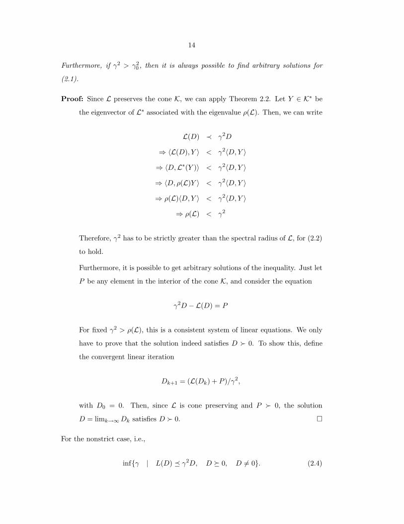
Furthermore, if γ2 > γ20 , then it is always possible to find arbitrary solutions for
(2.1).
Proof: Since L preserves the cone K, we can apply Theorem 2.2. Let Y ∈ K∗ be
the eigenvector of L∗ associated with the eigenvalue ρ(L). Then, we can write
L(D) ≺ γ2D
⇒ 〈L(D), Y 〉 < γ2〈D,Y 〉
⇒ 〈D,L∗(Y )〉 < γ2〈D,Y 〉
⇒ 〈D, ρ(L)Y 〉 < γ2〈D,Y 〉
⇒ ρ(L)〈D,Y 〉 < γ2〈D,Y 〉
⇒ ρ(L) < γ2
Therefore, γ2 has to be strictly greater than the spectral radius of L, for (2.2)
to hold.
Furthermore, it is possible to get arbitrary solutions of the inequality. Just let
P be any element in the interior of the cone K, and consider the equation
γ2D −L(D) = P
For fixed γ2 > ρ(L), this is a consistent system of linear equations. We only
have to prove that the solution indeed satisfies D 0. To show this, define
the convergent linear iteration
Dk+1 = (L(Dk) + P )/γ2,
with D0 = 0. Then, since L is cone preserving and P 0, the solution
D = limk→∞Dk satisfies D 0.
For the nonstrict case, i.e.,
infγ | L(D) γ2D, D 0, D 6= 0. (2.4)
15
under irreducibility assumptions, we have similarly the following theorem.
Theorem 2.5 Assume the operator L is cone-preserving and irreducible. Then, the
optimal solution of (2.4) is achieved, and has the value
γ20 = ρ(L). (2.5)
Proof: The proof is very similar to the previous one. For the first part, the condi-
tion Y 0 is guaranteed by the irreducibility of L. For the second part, the
optimal D can be taken to be equal to the eigenvector of L associated with
the spectral radius.
The results of Theorem 2.5 above also hold without the irreducibility assumption
on L. The proof uses a continuity argument, applying the theorem to the operator
L+ εP, with P a K-positive operator1, i.e., one that satisfies P(K − 0) ⊆ int K.
In this case, it is easy to show that L + εP is K-irreducible (since P is). Then we
just take the limit as ε→ 0, and use continuity of the spectral radius.
2.3.2 Computation
In the previous subsection a characterization of the optimal value as the spectral
radius of an operator was provided. Here we describe some approaches to the
problem of effectively computing the value of γ0.
The most straightforward way (although not the most efficient), is to compute
a matrix representation of the operator, and use a general purpose algorithm to
compute its eigenvalues. This is clearly not very convenient for large scale problems,
where Lanczos or Arnoldi methods are usually the best choice, especially if we are
interested only in a few eigenvalues/eigenvectors (as in the present case).
The use of a matrix representation also allows for “squaring”-type methods,
where a sequence of matrices A2k is used. This can be computed using the iteration
Ak+1 = A2k, with A0 = A and a suitable normalization scheme at each step. The
1Examples of positive operators for the nonnegative orthant and the positive semidefinite cone
are the matrix with all its elements equal to one, and the operator P(A) = trace(A)I, respectively.
16
effect of the squaring procedure is a separation of the eigenvalues depending on their
absolute value (since ρ(A2) = ρ2(A)).
Under a mild hypothesis (K-primitivity, a subset of K-irreducibility), it is possi-
ble to use power iteration-type methods to compute the spectral radius. Primitivity
is equivalent to requiring ρ(L) to be strictly greater than the magnitude of any
other eigenvalue [9]. It is always possible to obtain a primitive operator by small
perturbations of a non primitive one.
In this case, the simple iteration
Dk+1 = L(Dk)/‖L(Dk)‖
is guaranteed to converge to the eigenvector associated with the spectral radius (and
its norm to the optimal value), for every initial value D0 0. Note also that in the
primitive case the squaring procedure describe above result in a very efficient and
compact algorithm, since in this case Ak tends to a rank one matrix, from where
the spectral radius can be obtained immediately.
It should also be remarked that this power iteration approach to solve a par-
ticular type of LMIs has no relationship with the power-type algorithms usually
employed in the computation of µ lower bounds.
2.3.3 Applications
Lyapunov inequalities
A simple example, presented here mainly as an illustration of the results, is given
by the discrete time Lyapunov inequality, also known as the Stein inequality. This
is the LMI used to check stability of discrete time linear systems.
It takes the form
M∗XM −X < 0, X > 0, (2.6)
and it clearly has the required structure. Using the theory above, we obtain an
alternative proof of the well-known result that says that the LMI (2.6) is feasible if
and only if the spectral radius of M is less than one.
17
This example also shows an important point: even if the LMI we are directly
interested in does not have the cone-invariance property, if may be possible to
apply the preceding theory to an equivalent problem. As an illustration, consider
for example the continuous time Lyapunov LMI. It is well known that it can be
converted into the Stein equation, by the following transformations (β > 0 is not an
eigenvalue of A).
A∗P + PA < 0
⇐⇒ (A∗ + βI)P (A+ βI)− (A∗ − βI)P (A− βI) < 0
⇐⇒ (A∗ − βI)−1(A∗ + βI)P (A+ βI)(A − βI)−1 − P < 0
This is equivalent to defining M = (A+ βI)(A− βI)−1, the usual bilinear transfor-
mation between continuous and discrete domains, and checking for discrete stability.
It is also possible to study Riccati inequalities under a similar framework, at
least in the semidefinite case. The theory in this case requires some extensions of
the Perron–Frobenius setting to nonlinear operators (available in the literature).
This approach is not pursued further here.
Spherical µ upper bound LMI
It is possible to directly apply the results developed above to the computation of
the LMI upper bound for the generalizations of µ known as spherical µ [52]. In this
problem, Frobenius-like constraints are put on the uncertainty block ∆, as opposed
to induced norm constraints on each block. For simplicity, we will only refer only
to the scalar case.
More concretely, we want to obtain conditions that guarantee the well-posedness
of the feedback interconnection of a constant matrix M and a diagonal uncertainty
block ∆ = diagδ1, δ2, . . . , δn, δi ∈ C, that satisfies∑n
i=1 |δi|2 ≤ 1. As in the
standard case [69], necessary and sufficient conditions are computationally hard,
and therefore approximation methods should be used instead. Sufficient conditions
(given by µ upper bounds) are usually computed using LMI methods.
18
In this case, the underlying linear vector space is now the set of hermitian ma-
trices, and K will be the self-dual cone of positive semidefinite matrices. Note that
all the “vectors” in the preceding abstract setting are now matrices.
In the spherical µ upper bound case, the LMI to be solved is very similar to the
standard µ LMI upper bound (2.13).
M∗(P D)M − γ2D < 0, D > 0, (2.7)
where P is a positive definite matrix (equal to the identity, in the restricted case
presented above).
Lemma 2.6 Let P be positive semidefinite. Then, the operator L(D) = M∗(P
D)M preserves the cone K of positive semidefinite matrices.
Proof: L is the composition of the two operators L1(D) = P D and L2(D) =
M∗DM . The first one is cone-preserving by Theorem 2.1. The second one has
the same property, since x∗M∗DMx < 0 implies y∗Dy < 0, with y = Mx.
In the particular case where P is the identity, we obtain the following corollary:
Corollary 1 Let γ0 be the optimal solution of the GEVP:
γ04= infγ | M∗(I D)M − γ2D < 0, D > 0. (2.8)
Then,
γ20 = ρ(MT M∗).
Proof: A matrix representation of the nontrivial part (i.e., after removing the trivial
kernel) of the operator M∗(I D)M can easily be obtained by elementary
algebra (or, somewhat easier, using Kronecker products), to show the equality
diag(M∗(I D)M) = (MT M∗)diag(D),
where diag(D) is the operator that maps the diagonal elements of a matrix
into a vector.
19
The corollary shows that both the optimal value of γ and D can be obtained
by just solving one eigenvalue problem, with dimensions equal to those of M . Note
that the matrix MT M∗ is simply the matrix whose elements are the square of the
absolute value of the elements of M .
Rank minimization problem
In [63, 62], Mesbahi and Papavassilopoulos show that for certain special cases, the
rank minimization problem (which is computationally hard in general) can be re-
duced to a semidefinite program (an LMI). The structure of their problem can be
shown to be basically equivalent to the one presented here. Theorem 2.4 above can
be used to show that it is not even necessary to solve the resulting LMI, just solving
a linear system (using direct or iterative techniques, for example) will provide the
optimal solution. As in the previous subsection, the cone K in this problem is the
self-dual cone of positive semidefinite matrices.
The problem considered in [63, 62] is stated as:
min rank X
subject to: Q+M(X) 0
X 0,
where Q is a negative semidefinite matrix and M is a linear map of the structure
(called “type Z”)
M(X) = X −k∑i=1
MiXM′i .
Under these hypotheses, it is possible to prove [63, 62] that a solution can be
obtained by solving the associated LMI:
min trace X
subject to: Q+M(X) 0
X 0.
20
Let P = −Q (therefore P is positive semidefinite, i.e., P 0), and P 6= 0, to avoid
the trivial solution X = 0. Defining L(X) := X −M(X) =∑k
i=1MiXM′i , we
obtain the equivalent formulation:
min trace X (2.9)
subject to: X −L(X) P (2.10)
X 0. (2.11)
It is clear from its definition (and the proof of Lemma 2.6) that L(X) preserves the
cone of semidefinite positive matrices.
Theorem 2.7 If the LMIs (2.10-2.11) are feasible, then ρ(L) ≤ 1.
Proof: The proof is essentially similar to that of Theorem 2.4, taking γ = 1 and
using the condition P 0.
In the case ρ(L) < 1, then the constraint (2.11) is not binding at optimality, and
the solution can be obtained by solving the consistent linear system
X −L(X) = P, (2.12)
as the following theorem shows.
Theorem 2.8 Let Xe be the solution of (2.12). Then, Xe is an optimal solution of
the LMI (2.9-2.11).
Proof: Let’s show first that Xe 0. As in the proof of Theorem 2.4, consider the
sequence Xi, with X0 = 0 and Xi+1 = L(Xi) + P . All the elements in the
sequence belong to the cone K. The sequence converges (due to the spectral
radius condition), and limi→∞Xi = Xe. Closedness of K implies Xe ∈ K.
Let X be any feasible solution of the LMI. Therefore, we have:
Xe −L(Xe) = P,

21
X −L(X) P.
Subtracting, we obtain
X −Xe L(X −Xe),
and by repeated application of L to both sides of the inequality
X −Xe Lk(X −Xe), ∀k ≥ 1.
Since ρ(L) < 1, the right-hand side of the preceding inequality vanishes as
k →∞. This implies X −Xe 0, and therefore trace(X) ≥ trace(Xe).
Note: The case ρ(L) = 1 can also be analyzed, via perturbation arguments.
2.4 Additional comments and examples
In this section we give some examples on the irreducibility notion mentioned above,
and mention some of the applications of the results in the computation of approxi-
mate solutions for other LMIs that are not necessarily cone-preserving.
2.4.1 More on irreducibility
To explain a little bit more of the irreducibility concept introduced above, we will
present a couple of examples. In what follows, we will consider the GEVP problem
(2.8).
For the first case, take M to be
M =
1 1
0 0
According to Corollary 1, the optimal solution γ of the GEVP (2.7) (with P = I)
is given by the spectral radius of M∗ MT , which is γ0 = 1. In this case, the
22
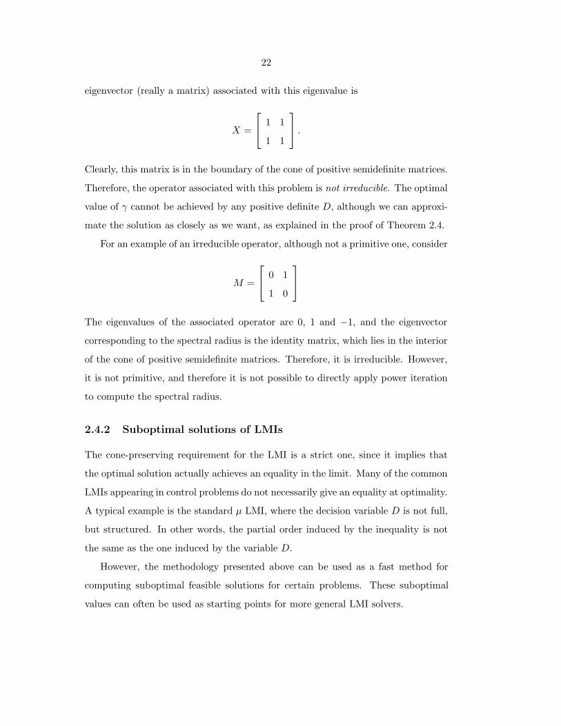
eigenvector (really a matrix) associated with this eigenvalue is
X =
1 1
1 1
.Clearly, this matrix is in the boundary of the cone of positive semidefinite matrices.
Therefore, the operator associated with this problem is not irreducible. The optimal
value of γ cannot be achieved by any positive definite D, although we can approxi-
mate the solution as closely as we want, as explained in the proof of Theorem 2.4.
For an example of an irreducible operator, although not a primitive one, consider
M =
0 1
1 0
The eigenvalues of the associated operator are 0, 1 and −1, and the eigenvector
corresponding to the spectral radius is the identity matrix, which lies in the interior
of the cone of positive semidefinite matrices. Therefore, it is irreducible. However,
it is not primitive, and therefore it is not possible to directly apply power iteration
to compute the spectral radius.
2.4.2 Suboptimal solutions of LMIs
The cone-preserving requirement for the LMI is a strict one, since it implies that
the optimal solution actually achieves an equality in the limit. Many of the common
LMIs appearing in control problems do not necessarily give an equality at optimality.
A typical example is the standard µ LMI, where the decision variable D is not full,
but structured. In other words, the partial order induced by the inequality is not
the same as the one induced by the variable D.
However, the methodology presented above can be used as a fast method for
computing suboptimal feasible solutions for certain problems. These suboptimal
values can often be used as starting points for more general LMI solvers.
23
For example, for the standard µ upper bound LMI
M∗(I D)M − γ2(I D) < 0, D > 0, (2.13)
it is possible to compute an approximate solution by using the following procedure:
1. Compute the exact solution γ21 ,D1 of the spherical µ LMI (2.7).
2. Compute the smallest η that satisfies
D1 ≤ η2(I D1). (2.14)
This is a generalized eigenvalue problem, that can be easily reduced to the
computation of the maximum eigenvalue of a hermitian matrix. It is also
possible to show, since D is positive definite, that η2 ≤ n [52].
3. Therefore, a suboptimal solution of the LMI is given by ID1, and the optimal
value is γ = ηγ1 ≤√nγ1.
Effectively, we have
M∗(I D1)M ≤ γ21D1 ≤ η2γ2
1(I D1).
It is possible to (almost) achieve the worst case difference between the optimal
solution and the approximate one (√n). For example, for the matrix
M =
1 ε · · · ε
ε ε · · · ε...
.... . .
...
ε ε · · · ε
,
with ε small, the optimal value of the LMI (2.13) is 1 + O(ε), but the fast upper
bound is approximately√n.
Another available procedure for computing fast solutions of the µ LMI is the
one due to Osborne [68]. A preliminary comparison made with random, normally
24
distributed matrices gives a slight advantage to the Osborne procedure. However,
the algorithm proposed can give better upper bounds (the opposite is also possible),
as the following example shows. For the matrix
M =
0 −9 −4
2 6 6
−3 −1 6
the µ upper bound computed by Osborne preconditioning is 10.321, and the bound
of the proposed procedure is 9.69 (the value of the LMI upper bound is 9.6604, and
is in fact equal to µ since there are three blocks).
2.4.3 Examples
As a simple example of the computational advantages of the proposed formulation,
we will compare the effort required to compute solutions of the spherical µ LMI
upper bound(2.7), for a given problem.
We take M to be a 16 × 16 complex matrix, randomly generated. The com-
putation of the optimal value of the LMI (2.7) with a general purpose LMI solver
for MATLAB [35] and a tolerance set to 10−4 requires (on a Sun Ultra 1 140) ap-
proximately 160 seconds. By using the procedure presented here, either by power
iteration or explicitly computing the eigenvalues, the result can be obtained in less
than one second.

25
Chapter 3
Efficient solutions for KYP-based LMIs
The semidefinite programs appearing in linear robustness analysis problems usually
have a very particular structure. This special form is a consequence of both the
linearity and the time invariance of the underlying system. In this chapter, we
will see how this special structure can be exploited in the formulation of efficient
algorithms.
The KYP lemma (Kalman-Yakubovich-Popov [93], see [77] for an elementary
proof) establishes the equivalence between a frequency domain inequality and the
feasibility of a particular kind of LMI (linear matrix inequality). It is an important
generalization of classical linear control results, such as the bounded real and positive
real lemma. It is also a fundamental tool in the practical application of the IQC
(integral quadratic constraints) framework [61] to the analysis of uncertain systems.
The theorem replaces an infinite family of LMIs, parameterized by ω, by a finite
dimensional problem. This is extremely useful from a practical viewpoint, since it
allows for the use of standard finite dimensional LMI solvers.
However, in the case of systems with large state dimension n, the KYP approach
is not very efficient, since the matrix variable P appearing in the LMI (3.2) has
(n2 +n)/2 components, and therefore the computational requirements are quite big,
even for medium sized problems. For example, for a problem with a plant having
100 states (which is not uncommon in certain applications), the resulting problem
has more than 5000 variables, beyond the limits of what can be currently solved
26
with reasonable time and space requirements using general-purpose LMI software.
In this chapter, we present an efficient algorithm for the solution of this type of
inequalities. The approach is an outer approximation method [72], and is based on
the algorithms used in the computation of H∞ system norms. The idea is to impose
the frequency domain inequality (3.1) only at a discrete number of frequencies.
These frequencies are then updated by a mechanism reminiscent of those used in
H∞ norm computation.
Previous related work includes of course the literature on the computation ofH∞system norms. In particular, references [16, 20, 15] developed quadratically conver-
gent algorithms, based explicitly on the Hamiltonian approach. Also, a somewhat
related approach in [60] implements a cutting-plane based algorithm, where linear
constraints are imposed on the optimization variables.
3.1 The KYP lemma
In this section we review some basic linear algebra facts, and also present a version
of the KYP lemma. The notation is standard.
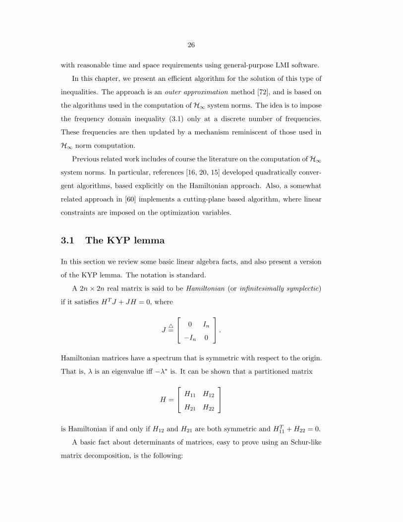
A 2n× 2n real matrix is said to be Hamiltonian (or infinitesimally symplectic)
if it satisfies HTJ + JH = 0, where
J4=
0 In
−In 0
.Hamiltonian matrices have a spectrum that is symmetric with respect to the origin.
That is, λ is an eigenvalue iff −λ∗ is. It can be shown that a partitioned matrix
H =
H11 H12
H21 H22
is Hamiltonian if and only if H12 and H21 are both symmetric and HT
11 +H22 = 0.
A basic fact about determinants of matrices, easy to prove using an Schur-like
matrix decomposition, is the following:
27
Lemma 3.1 Let Q be a partitioned matrix
Q =
Q11 Q12
Q21 Q22
with Q11 and Q22 invertible. Then, we have the identity:
detQ = detQ11 det(Q22 −Q21Q−111 Q12) = detQ22 det(Q11 −Q12Q
−122 Q21)
A fairly general version of the KYP lemma, as presented in [77] is the following:
Theorem 3.2 Let A ∈ Rn×n, B ∈ Rn×m,M = MT ∈ R(n+m)×(n+m), with A having
no purely imaginary eigenvalues. Then, the two following statements are equivalent:
1.
F (jω)4=
(jωI −A)−1B
I
∗M (jωI −A)−1B
I
< 0, ∀ω ∈ R ∪ ∞
(3.1)
2. There exists a symmetric n× n matrix P that satisfies
ATP + PA PB
BTP 0
+M < 0 (3.2)
Proof: We present a proof of (2) ⇒ (1), to show the connection with the methods
of Chapter 4. The second condition guarantees M22 < 0, so the case ω = ∞
holds. In what follows, we analyze the case ω 6=∞.
An equivalent statement of (3.1) is the implication
jωx = Ax+Bu =⇒
x
u
∗M x
u
< 0.
28
Let P be a symmetric matrix. Clearly, a condition that guarantees that the
expression above holds is:
x∗P (Ax+Bu− jωx) + (Ax+Bu− jωx)∗Px+
x
u
∗M x
u
< 0,
for all x ∈ Rn, u ∈ Rm, (x, u) 6= 0. It can be easily verified that the terms
containing ω cancel, and the expression can be rewritten as (3.2).
For a proof of the other direction (1 ⇒ 2), see [77].
In the application of this result to the stability analysis of uncertain systems,
the matrix M depends affinely on some parameter vector x. These are the variables
of the LMI optimization problem, where we try to minimize some linear function
of x over the feasible set (for example, a bound on the L2-induced norm). In what
follows, the dependence on x is usually omitted, for notational reasons.
Here we will deal only with the strict version of the KYP lemma, i.e., with a
strict inequality in (3.1), (3.2). The reason is twofold: in the first place, no control-
lability/stabilizability assumptions are necessary, simplifying the proofs. Secondly,
since the resulting LMIs will in general be solved using interior-point methods, the
existence of a strictly feasible solution is usually guaranteed.
3.2 The Algorithm
The basic idea is to replace the semi-infinite optimization problem (3.1) by a finite
dimensional relaxation. We choose to impose the constraint only at a finite number
of frequencies ωk ∈ Ω (see [50] for a related approach). For a given ω, equation (3.1)
is an LMI in M .
A high-level description of the algorithm follows:
Algorithm 1
1. Initialize the set of frequencies Ω4= 0.
2. Solve (3.1) with the current Ω set.

29
3. Find a frequency ωk where the constraint (3.1) is violated (up to an ε toler-
ance). If no such frequency exists, exit.
4. Add that frequency to the set Ω, and go to step 2.
As we can see, the underlying idea of an outer approximation algorithm is a
generalization of a cutting plane method [72]. We replace the description of the
feasible set by a convenient relaxation. If the resulting solution does not satisfy the
original constraints, a cutting plane (in this case, a possibly curved hypersurface)
that separates that solution from the true feasible set is added. The process is
repeated until the desired tolerance is reached.
As in the case of H∞ norm computation [16, 20], the effectiveness of the algo-
rithm hinges on the possibility of detecting in an efficient manner the frequencies
at which the inequality is violated. To this end, define the 2n × 2n Hamiltonian
matrix:
H =
A−BM−122 M21 −BM−1
22 BT
−M11 +M12M−122 M21 −AT +M12M
−122 B
T
(3.3)
It can be shown (see for example [93]) that the conditions (3.1), (3.2) are satisfied
if and only if M22 < 0 and H has no imaginary eigenvalues. In this case, it is
possible to obtain a solution P of the LMI (3.1) by computing a solution of the
Riccati equation associated with the Hamiltonian (or a suitable perturbation, if the
subspace complementarity condition is not satisfied). If the eigenvalue condition is
violated, then there is a relationship between the critical frequencies, as the following
theorem shows.
Theorem 3.3 Assume M22 < 0. Then, F (jω0) is singular, if and only if jω0 is an
imaginary eigenvalue of H.
Proof: Consider the partitioned matrix
Q4=
jωI −A 0 −B
M11 jωI +AT M12
M21 BT M22
.
30
The diagonal submatrices are invertible, since A has no imaginary eigenvalues
and M22 < 0. Applying Lemma 3.1, we immediately have the identity
det(jωI −H) detM22 = det(jωI +AT ) detF (jω) det(jωI −A)
from where the result follows.
Special cases of this theorem are the ones used in [16] to compute the H∞ norm
or the minimum dissipation of a transfer function.
Several options are available for the choice of the frequency to add to the set
Ω. A particularly good one is to choose ωk as the frequency at which F (jω) is
maximally positive (i.e., where its first singular value achieves its maximum over
frequency). This can be obtained at a computational cost similar to that of an
H∞ norm. In the following section we present a convergence argument for the
procedure resulting from this choice. A cheaper alternative is to pick a criterion
similar to the one used in [20]. Given the imaginary eigenvalues of H, consider the
midpoint frequencies, and choose the one where the constraint is most violated. The
computational requirements of this step are minimal, compared to the one required
to solve the LMIs.
An important difference of the LMI case discussed here with the simpler H∞norm case (where the only LMI variable is the KYP one) is that at optimality more
than one constraint can be active. In fact, the results in [50] show that at most
n+ 1 frequencies are active, where n is the number of IQCs.
In the algorithm as described, no constraint dropping occurs. That is, we keep
adding constraints, until convergence. Since we know a priori a bound on the
number of active constraints, dropping old, non-binding constraints seems a natural
idea.
The distinctive feature of the algorithm is that the KYP variable P , never ap-
pears explicitly in the procedure. Nevertheless, as mentioned before, it is possible
to compute its value after the problem is solved, at a computational cost similar to
solving a Riccati equation.
31
A somewhat related approach is used in [60], where the eigenvectors of the
Hamiltonian are used to construct linear constraints for the elements of M . In our
approach, the constraints are matrix valued (not linear) and we do not impose the
restrictions directly at the critical frequencies, but at other points where they are
more violated. This way, convergence should be improved (in the H∞ case, it is
even quadratic).
3.2.1 Convergence
It is possible to prove convergence of the first version of the algorithm. This corre-
sponds to the choice of ωk as the point at which the frequency domain inequality is
maximally violated. In fact, for this variation we can apply the results on the con-
vergence of more abstract version of the outer approximation method (Conceptual
Algorithm 3.5.19 in [72]).
It is possible to show (see [72]) that if the algorithm produces a infinite sequence
of solutions, then any accumulation point of this sequence is a global solution of the
original problem. The infinite set of frequency constraints can be “compactified”
either by considering the extended real line or by a standard bilinear transformation.
Currently we do not have explicit, nonconservative expressions for the conver-
gence rate. This seems to be a general feature of the outer approximation class of
algorithms, since even for cutting plane methods the known theoretical bounds are
usually extremely conservative, when compared to the actual performance.
3.3 Using the dual
A not so convenient feature of the presented approach is that a new constraint is
added at each iteration. This implies that the previous solution will not be primal
feasible, forcing a restart of the optimization, unless an infeasible start method is
used.
This can be solved by focusing instead on the dual optimization problem, as is
well known from the linear programming literature, for instance. In this case, new
32
∆
G uy
wv
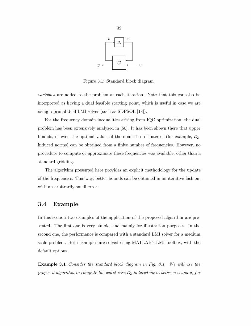
Figure 3.1: Standard block diagram.
variables are added to the problem at each iteration. Note that this can also be
interpreted as having a dual feasible starting point, which is useful in case we are
using a primal-dual LMI solver (such as SDPSOL [18]).
For the frequency domain inequalities arising from IQC optimization, the dual
problem has been extensively analyzed in [50]. It has been shown there that upper
bounds, or even the optimal value, of the quantities of interest (for example, L2-
induced norms) can be obtained from a finite number of frequencies. However, no
procedure to compute or approximate these frequencies was available, other than a
standard gridding.
The algorithm presented here provides an explicit methodology for the update
of the frequencies. This way, better bounds can be obtained in an iterative fashion,
with an arbitrarily small error.
3.4 Example
In this section two examples of the application of the proposed algorithm are pre-
sented. The first one is very simple, and mainly for illustration purposes. In the
second one, the performance is compared with a standard LMI solver for a medium
scale problem. Both examples are solved using MATLAB’s LMI toolbox, with the
default options.
Example 3.1 Consider the standard block diagram in Fig. 3.1. We will use the
proposed algorithm to compute the worst case L2 induced norm between u and y, for

33
Frequencies Obj. Value Imag. Eigs. of H
0 2.0012 0.0353 1.9984
0 1.0169 2.7282 1.0171 1.2073
0 1.0169 1.1122 2.7474 -
Table 3.1: Numerical values for Example 3.1.
0 1 2 3 4 5 6 7 8−2
−1.5
−1
−0.5
0
0.5
Frequency ω
F(jω
) First
SecondThird
Figure 3.2: Frequency domain plots corresponding to Example 3.1.
the plant given by
G =
s+1s2+2s+2 1
1 0
.The ∆ block is an uncertain contractive LTV operator, and therefore satisfies the
IQC given by
Π(jω) =
1 0
0 −1
.The results of the sequence of subproblems are shown in Table 3.1 and Fig. 3.2.
As we can see, on the third and last iteration we obtain a value of the parameters
that makes the frequency domain inequality to be satisfied. That makes possible, if
34
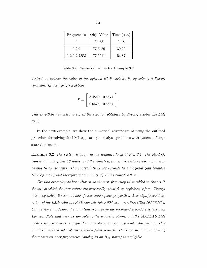
Frequencies Obj. Value Time (sec.)
0 64.33 14.8
0 2.9 77.3456 30.29
0 2.9 2.7353 77.5511 54.87
Table 3.2: Numerical values for Example 3.2.
desired, to recover the value of the optimal KYP variable P , by solving a Riccati
equation. In this case, we obtain
P =
3.4849 0.6674
0.6674 0.6644
.This is within numerical error of the solution obtained by directly solving the LMI
(3.1).
In the next example, we show the numerical advantages of using the outlined
procedure for solving the LMIs appearing in analysis problems with systems of large
state dimension.
Example 3.2 The system is again in the standard form of Fig. 3.1. The plant G,
chosen randomly, has 50 states, and the signals u, y, v, w are vector-valued, with each
having 10 components. The uncertainty ∆ corresponds to a diagonal gain bounded
LTV operator, and therefore there are 10 IQCs associated with it.
For this example, we have chosen as the new frequency to be added to the set Ω
the one at which the constraints are maximally violated, as explained before. Though
more expensive, it seems to have faster convergence properties. A straightforward so-
lution of the LMIs with the KYP variable takes 996 sec., on a Sun Ultra 10/300Mhz.
On the same hardware, the total time required by the presented procedure is less than
120 sec. Note that here we are solving the primal problem, and the MATLAB LMI
toolbox uses a projective algorithm, and does not use any dual information. This
implies that each subproblem is solved from scratch. The time spent in computing
the maximum over frequencies (analog to an H∞ norm) is negligible.
35
0 5 10 15 20 25−200
0
200
400
600
800
1000
Frequency ω
Max
imum
eig
enva
lue
of F
(jω)
First
SecondThird
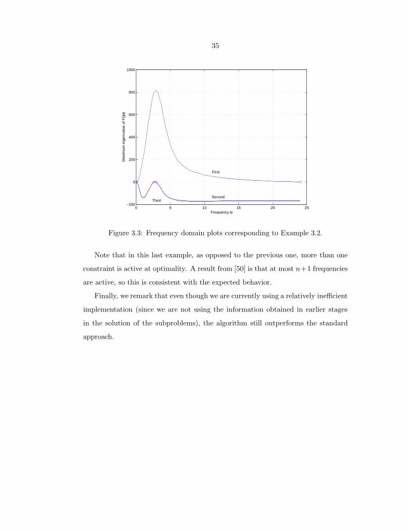
Figure 3.3: Frequency domain plots corresponding to Example 3.2.
Note that in this last example, as opposed to the previous one, more than one
constraint is active at optimality. A result from [50] is that at most n+1 frequencies
are active, so this is consistent with the expected behavior.
Finally, we remark that even though we are currently using a relatively inefficient
implementation (since we are not using the information obtained in earlier stages
in the solution of the subproblems), the algorithm still outperforms the standard
approach.

36
37
Chapter 4
Sums of squares and algebraic geometry
This chapter presents our approach to the formulation of stronger convex conditions
for a large class of optimization and systems and control problems. The fundamen-
tal feature is the computational tractability of the sum of squares decomposition
for multivariable polynomials. As shown below, the problem can be solved via
semidefinite programming methods.
Complementing this formulation with results in semialgebraic geometry (the
Positivstellensatz), a whole class of convex approximations for optimization prob-
lems is developed. In subsequent chapters, we specialize the techniques to some
specific problems.
4.1 Global nonnegativity
A basic problem that appears in many areas of mathematics is that of checking
global nonnegativity of a function of several variables. Concretely, the problem is to
give equivalent conditions or a procedure for checking the validity of the proposition
F (x1, . . . , xn) ≥ 0, ∀x1, . . . , xn ∈ R. (4.1)
This is a very important problem, and lots of research efforts have been devoted
to it. In order to study the problem from an algorithmic approach, we need to
put further restrictions on the class of functions F , since the general question can
38
be shown to be undecidable. To illustrate this, consider Richardson’s theorem, as
quoted in [71].
Theorem 4.1 Let R consist of the class of expressions generated by
1. The rational numbers and the two real numbers π and ln 2.
2. The variable x.
3. The operations of addition, multiplication, and composition.
4. The sine, exponential, and absolute value functions.
If E ∈ R, the predicate “E = 0” is recursively undecidable.
It is clear then that we necessarily need to limit the structure of the possible
functions F , while at the same time making the problem general enough to guarantee
the applicability of the results. A good compromise is achieved by considering the
case of polynomial functions.
Definition 4.1 A polynomial f in x1, . . . , xn with coefficients in a field k is a finite
linear combination of monomials:
f =∑α
cαxα =
∑α
cαxα11 . . . xαnn , cα ∈ k, (4.2)
where the sum is over a finite number of n-tuples α = (α1, . . . , αn), αi ∈ N0. The
set of all polynomials in x1, . . . , xn with coefficients in k is denoted k[x1, . . . , xn].
Definition 4.2 A form is a polynomial where all the monomials have the same
degree d :=∑
i αi. In this case, the polynomial is homogeneous of degree d, since it
satisfies f(λx1, . . . , λxn) = λdf(x1, . . . , xn).
Many concrete problems, particularly in systems and control, can be reduced
to the verification of the global nonnegativity of a polynomial function [13]. Some
examples, presented in Chapter 7, are Lyapunov function computation, output feed-
back stabilization, multidimensional system stability, etc.

39
As mentioned in Chapter 1, the Tarski-Seidenberg decision procedure [12, 64, 13]
provides in this case an explicit algorithm for deciding if (4.1) holds, so we know
that the problem is decidable. There are also a few alternative approaches, also
based in decision algebra; see [13] for a survey of existing techniques.
It is possible to show that the general problem of testing global positivity of a
polynomial function is in fact NP-hard (when the degree is at least four). Therefore,
(unless P=NP) any method guaranteed to obtain the right answer in every possible
instance will have unacceptable behavior for a problem with a large number of
variables. This is the main drawback of theoretically powerful methodologies such
as quantifier elimination [31, 47].
If we want to avoid the inherent complexity problems related with the exact
solution, the question arises: are there any conditions, that can be tested in poly-
nomial time, to guarantee global positivity of a function? As we will shortly see,
one such condition is given by the existence of a sum of squares decomposition.
4.2 Sums of squares
If a polynomial F satisfies (4.1), then an obvious necessary condition is that the
degree of the polynomial (or form, in the homogeneous case) be even. A decep-
tively simple sufficient condition for a real-valued function F (x) to be nonnegative
everywhere is given by the existence of a sum of squares decomposition:
F (x) =∑i
f2i (x)
It is clear that if a given function F (x) can be written as above, for some fi, then
it is nonnegative for all values of x.
However, the question immediately arises: when is such decomposition possible?
Naturally, in order for the problem to make sense, some restriction on the class of
functions fi has to be imposed again. Otherwise, we can always define f1 to be the
square root of F , making the condition both useless and trivial.
For the case of polynomials, this is a well-analyzed problem, first studied by
40
David Hilbert more than a century ago. In fact, one of the questions in his famous
list of twenty-three unsolved problems presented at the International Congress of
Mathematicians at Paris in 1900, deals with the representation of a definite form as
a sum of squares of rational functions.
For notational simplicity, we will use the notation psd for “positive semidefinite”
and sos for “sum of squares.” Following the notation in references [24, 80], let Pn,m
be the set of psd forms of degree m in n variables, and Σn,m the set of forms p such
that p =∑
k h2k, where hk are forms of degree m/2.
Hilbert himself noted that not every psd polynomial (or form) is sos. A simple,
more modern counterexample is the Motzkin form (here, for n = 3)
M(x, y, z) = x4y2 + x2y4 + z6 − 3x2y2z2 (4.3)
Positive semidefiniteness can be easily shown using the arithmetic-geometric inequal-
ity, and the nonexistence of a sos decomposition follows from standard algebraic
manipulations (see [80] for details), or the procedure outlined below (Example 4.5).
Hilbert gave a complete characterization of when these two classes are equiv-
alent. There are three cases for which the equality holds. The first one, is the
case of forms in two variables (n = 2), which are equivalent by dehomogenization
to polynomials in one variable. This is easy to show using a factorization of the
polynomial in linear and quadratic factors. The second one is the familiar case of
quadratic forms (i.e., m = 2) where the sum of squares decomposition follows from
the eigenvalue/eigenvector factorization. There is also a surprising third case, where
P3,4 = Σ3,4, corresponding to quartic forms in three variables.
The sum of squares decomposition is the underlying machinery in Shor’s global
bound for polynomial functions [91], as is explicitly mentioned in [83]. It has also
been presented as the “Gram matrix” method in [24] and more recently in [74],
although no mention to interior point methods is made: the resulting LMIs are
solved via decision methods. A related scheme also appears in [41] (note also the
important correction in [33]).
41
The basic idea of the method is the following: express the given polynomial as a
quadratic form in some new variables z. These new variables are the original x ones,
plus all the monomials of degree less than or equal to m/2 given by the different
products of the x variables. Therefore, F (x) can be represented as:
F (x) = zTQz (4.4)
where Q is a constant matrix. If in the representation above Q is positive semidefi-
nite, then F (x) is also psd. This is the idea in [14], for example, and it can be shown
to be conservative, generally speaking. The main reason is that since the variables
zi are not independent, the representation (4.4) might not be unique, and Q may be
psd for some representations but not for others. Similar issues appear in the anal-
ysis of quasi-LPV systems; see [45]. By using identically satisfied constraints that
relate the zi variables among themselves (of the form zizj = zkzl or z2i = zkzl), it is
easily shown that there is a linear subspace of matrices Q that satisfy (4.4). If the
intersection of this subspace with the positive semidefinite matrix cone is nonempty,
then the original function F is guaranteed to be sos (and therefore psd). This fol-
lows from an eigenvalue decomposition of Q = T TDT, di ≥ 0, which implies the sos
F (x) =∑
i di(Tz)2i . Conversely, if F can indeed be written as the sum of squares
of polynomials, then expanding in monomials will provide the representation (4.4).
Example 4.1 Consider the quartic form in two variables described below, and de-
fine z1 := x21, z2 := x2
2, z3 := x1x2:
F (x1, x2) = 2x41 + 2x3
1x2 − x21x
22 + 5x4
2
=
x2
1
x22
x1x2
T
2 0 1
0 5 0
1 0 −1
x21
x22
x1x2
=
x2
1
x22
x1x2
T
2 −λ 1
−λ 5 0
1 0 −1 + 2λ
x21
x22
x1x2
.

42
Take for instance λ = 3. In this case,
Q = LTL, L =1√2
2 −3 1
0 1 3
And therefore we have the sum of squares decomposition:
F (x1, x2) =12
((2x21 − 3x2
2 + x1x2)2 + (x22 + 3x1x2)2).
Example 4.2 The following example is from [13, Example 2.4], where it is required
to find whether or not the quartic polynomial,
P (x1, x2, x3) = x41 − (2x2x3 + 1)x2
1 + (x22x
23 + 2x2x3 + 2),
is positive definite. In [13], this property is established using decision algebra.
By constructing the Q matrix as described above, and solving the corresponding
LMIs, we obtain the sums of squares decomposition:
P (x1, x2, x3) = 1 + x21 + (1− x2
1 + x2x3)2,
that immediately establishes global positivity. Notice that the decomposition actually
proves a stronger fact, namely that P (x1, x2, x3) ≥ 1 for all values of xi. In fact,
the bound can be shown to be exact, since for example P (0, 1,−1) = 1.
If the polynomial F is sparse, in the sense that many of the monomials are zero,
then it is usually possible to considerably simplify the resulting LMIs. To do this,
we can use a result, first formulated in [78], that characterizes the monomials that
can appear in a sum of squares representation. Define the cage (or Newton polytope
[87]) of F as the integer lattice points in the convex hull of the degrees α (in 4.2),
considered as vectors in Rn. Then, it can be shown that the only monomials xβ
that can appear in a sum of squares representation are those such that 2β is in the
43
cage of F .
The most important properties that distinguish the semidefinite programming
condition from other approaches to the polynomial nonnegativity problem are its
relative tractability, and the fact that it can be easily extended to the uncertain case
(i.e., when we are looking for a psd F , subject to additional conditions). This last
feature will prove to be critical in the application to the theory to many control
related problems.
As an example, we can apply the technique to compute global lower bounds for
polynomial functions [83]. Since the condition
(F (x)− γ) is a sum of squares
is affine in γ, then it is possible to efficiently compute the maximum value of γ for
which this property holds. In some cases, as in Example 4.2 above, the resulting
bound is optimal. However, for the reasons mentioned earlier, it is also possible to
obtain conservative results.
Example 4.3 As examples of a problem with nonzero gaps, we compute global lower
bounds of dehomogenizations of the Motzkin polynomial M(x, y, z) presented in (4.3)
above. Since M(x, y, z) is nonnegative, its dehomogenizations also have the same
property. Furthermore, since M(1, 1, 1) = 0, they always achieve its minimum
possible value.
Fixing the variable y, we obtain
F (x, z) := M(x, 1, z) = x4 + x2 + z6 − 3x2z2.
To obtain a lower bound, we search for the maximum γ for which F (x, z) − γ is a
sum of squares.
Solving the corresponding LMIs, the best lower bound that can be obtained this
way can be shown to be − 7294096 ≈ −0.177978, and follows from the decomposition:
F (x, z) + 7294096 = (−9
8z + z3)2 + (2764 + x2 − 3
2z2)2 + 5
32x2

44
The gap can also be infinite, for some particular problems. Consider the deho-
mogenization in z:
G(x, y) := M(x, y, 1) = x4y2 + x2y4 + 1− 3x2y2.
It can be shown that G(x, y) − γ is not a sum of squares for any value of γ, and
therefore no useful information can be obtained in this case. Fortunately, techniques
are available to deal with such cases, as we will shortly see.
4.3 The dual problem
It is enlightening to analyze the dual problem, that gives conditions on when F (x)
is not a sum of squares. Given F (x), consider a representation
F (x) = zTQz = trace zzTQ,
for all vectors z. Relaxing the rank one constraint on the matrix W := zzT (now
W is only positive semidefinite), it is clear that a sufficient condition for F (x) not
to be a sum of squares is the existence of a matrix W satisfying
trace WQ < 0, W ≥ 0.
The non uniqueness of Q in the quadratic representation now translates into equality
constraints between the elements of W . These equality constraints ensure that
products between the newly defined variables that are supposed to be identical
actually have the same value.
Example 4.4 Consider again Example 4.1. In this case, the dual variable is:
W =
w11 w12 w13
w12 w22 w23
w13 w23 w33
=
z2
1 z1z2 z1z3
z1z2 z22 z2z3
z1z3 z2z3 z23
, (4.5)
45
and the constraint that z1z2 = z23 translates into the condition w12 = w33.
The dual problem gives direct insight in the process of checking, after solving the
LMIs, if the relaxation was exact. In this case, under no degeneracies, the optimal
W matrix will have rank one, and the components of the corresponding eigenvector
will verify the constraints satified by the zi variables.
It should be noted that, at least in principle, the method has some degree of
conservativeness. As explained above, this is because the class of psd polynomials
is not equal to the sos ones. It is not clear yet how relevant this gap is in prac-
tical terms. After all, almost every time the positivity of a function needs to be
established (for example, backstepping methods in control theory), this is usually
done by constructing a sos representation, either implicitly or explicitly. In any
case, there are possible workarounds, at some computational cost. For a psd F (x),
Artin’s positive answer to Hilbert’s 17th problem assures the existence of a polyno-
mial G(x), such that F (x)G2(x) can be written as a sum of squares. In particular,
Reznick’s results [79] show that if F is positive definite it is always possible to take
G(x) = (∑x2i )r, for sufficiently large r.
Example 4.5 Consider the case of the Motzkin form given in equation (4.3). As
mentioned before, it cannot be written as a sum of squares of polynomials. Even
though it is only semidefinite (so in principle we cannot apply Reznick’s theorem),
after solving the LMIs we obtain the decomposition:
(x2 + y2 + z2)M(x, y, z) = (x2yz − yz3)2 + (xy2z − xz3)2 + (x2y2 − z4)2 +
+14
(xy3 − x3y)2 +34
(xy3 + x3y − 2xyz2)2,
from where nonnegativity is obvious. When applying this improved method to the
problems with nonzero gaps in Example 4.3, exact solutions are obtained.
Additional stronger conditions can be obtained using the Positivstellensatz pre-
sented in Section 4.4.2 below.
46
4.3.1 Computational considerations
The computational cost of the procedure clearly depends on both the degree of the
polynomial, and the number of variables. The number of monomials of degree less
than or equal to m/2 (m is even) is Nz :=(n−1+m/2
m/2
). This is the size of the resulting
LMI, assuming no simplifications occur, which is not usually the case. The number
of constraints (additional variables in the LMIs) can be large, especially when using
many variables and high degree polynomials. For a fixed degree, however, that
number is always a polynomial expression in n (it is always bounded by N2z , for
instance).
4.4 Algebraic geometry
At its most basic level, algebraic geometry deals with the study of the solution set of
a system of polynomial equations. From a more general viewpoint, it focuses on the
close relationship between geometric objects and the associated abstract algebraic
structures. It is a subject with a long and illustrious history, and many links to
seemingly unconnected areas of mathematics, such as number theory.
Increasingly important in the last decades is the fact that new algorithms and
methodologies (for instance, Grobner basis) have enabled the study of very compli-
cated problems, not amenable to paper and pencil calculations.
In this section, some critical elements from algebraic geometry theory are pre-
sented. The usual name for the specific class of theorems we introduce is Stellensatze,
from the German words Stellen (places) and Satz (theorem). The first such result
was proved by Hilbert, and deals with the case of an algebraically closed field such
as C. When we are interested only in real roots, we need to introduce the Artin-
Schreier theory of formally real fields, that was developed along the search for a
solution of Hilbert’s 17th problem.

47
4.4.1 Hilbert’s Nullstellensatz
The theorem below establishes a correspondence between a geometric object (an
affine variety) and an algebraic concept, a polynomial ideal. Hilbert’s Nullstellen-
satz basically establishes that in an algebraically closed field, the only ideal that
represents the empty variety is the entire polynomial ring.
Theorem 4.2 (Hilbert’s Nullstellensatz) Let k be an algebraically closed field
(such as C) and let I ⊂ k[x1, . . . , xn] be an ideal satisfying V(I) = ∅. Then 1 ∈ I,
or equivalently, I = k[x1, . . . , xn].
The Nullstellensatz can be applied to show the nonexistence of solutions for a
given system of polynomial equations
fi(x) = 0, i = 1, . . . ,m, x ∈ Cn. (4.6)
To do this, we need to show that the corresponding variety is empty. Using the
Nullstellensatz, this is equivalent to verifying that the identity polynomial is in the
ideal generated by the given equations. In other words, we need to find polynomials
gi such that
f1(x)g1(x) + · · ·+ fm(x)gm(x) = 1. (4.7)
The sufficiency of the condition should be obvious. If the equality above is
actually satisfied for some polynomials gi, and assuming there exists a point x0 in
the variety, after evaluating (4.7) at x0 we immediately reach the contradiction 0=1.
Remark 4.1 In the case when i = 2, and the fi are elements of the ring of stable
and proper transfer functions, the Nullstellensatz reduces to the Bezout identity
used in the coprime factorization approach to feedback stabilization. In that case,
the nonexistence of common zeros can be interpreted as the lack of unstable pole/zero
cancellations.
The polynomials gi provide a certificate (usually called a Nullstellensatz refuta-
tion) that the variety described by (4.6) is empty. Given the gi, the equality (4.7)
48
can be checked in a number of operations that is polynomial in their length (if we
only count real operations, in the number of nonzero coefficients).
There are at least two possible approaches to effectively find polynomials gi.
The first one depends on having explicit bounds on the degree of the products figi.
A number of such bounds are available in the literature, see for instance [19, 53, 7].
For example, if the polynomials fi(x) have maximum degree d, and x ∈ Cn, then
the bound
degfigi ≤ max(3, d)n
holds. The bound is tight, in the sense that there exist specific examples of systems
for which the expression above is an equality.
Given a upper bound on the degree, and a parameterization of the unknown
polynomials gi, then a solution can be obtained by solving a system of linear equa-
tions.
The other procedure is based on Grobner basis methods [26, 64]. By Hilbert’s
Basis theorem, every polynomial ideal is finitely generated. Grobner bases provide a
computationally convenient representation for a set of generating polynomials of an
ideal. For example, for the case of degree one (only linear terms), and a lexicographic
term ordering, a Grobner basis is basically equivalent to Gaussian elimination. If
the variety is empty, the corresponding basis has only one element, the identity
polynomial. As a byproduct of the computation of a Grobner basis, it is possible to
explicitly obtain the polynomials gi.
Example 4.6 As an example of a Nullstellensatz refutation, we will prove that the
following system of polynomial inequalities does not have solutions over C.
f1(x) := x2 + y2 − 1 = 0
f2(x) := x+ y = 0
f3(x) := 2x3 + y3 + 1 = 0
49
To show this, consider the polynomials
g1(x) := 17(1− 16x− 12y − 8xy − 6y2)
g2(x) := 17(−7y − x+ 4y2 − 16 + 12xy + 2y3 + 6y2x)
g3(x) := 17(8 + 4y)
After simple algebraic manipulations, we can verify that
f1g1 + f2g2 + f3g3 = 1,
proving the nonexistence of solutions over C.
Example 4.7 (Modus ponens) The modus ponens is a basic rule of inference
for propositional logic. It establishes that from the truth of the statements A and
A→ B, we can conclude that B is also true.
It is possible to give an algebraic “translation” of the modus ponens rule. For
example, for the case of three propositions, we have that the statements
P1, P1 → P2, P2 → P3, ¬P3,
cannot all be true simultaneously. Let the variables xi ∈ 0, 1 (this can be dealt
with by adding the constraints xi(1 − xi) = 0). Associating the “truth” of Pi to
the variable xi taking the value one, then the modus ponens is equivalent to the
nonexistence of a common solution of the equations fi(x) = 0, where
f1(x) := 1− x1 (4.8)
f2(x) := x1(1− x2) (4.9)
f3(x) := x2(1− x3) (4.10)
f4(x) := x3 (4.11)
An algebraic proof of the validity of the modus ponens in this case is given by the

50
identity:
(1− x2)f1 + f2 + f3 + x2f4 = 1.
It can be shown [22] that in the general case of n variables, the minimum degree of
the required Nullstellensatz refutation is approximately log n, with the result being
tight.
An equivalent statement of the Nullstellensatz is in an ideal-theoretic formula-
tion. Let I(V ) be the polynomial ideal associated with a given algebraic variety,
and V(I) the variety generated by the ideal I (see Appendix A). In this case, given
a polynomial ideal I, a concise statement of the (strong) Nullstellensatz is
I(V(I)) =√I,
where√I is the radical of I.
In many cases, we need to verify if a polynomial f vanishes on a given algebraic
variety V . In algebraic terms, this turns out to be equivalent to the radical member-
ship problem: does f belong to the radical of the ideal associated with the variety
V ? By introducing a slack variable and applying Theorem 4.2, the characterization
below can be obtained [26].
Theorem 4.3 Let k be an algebraically closed field. If f, f1, . . . , fm ∈ k[x1, . . . , xn]
are such that
f1(x) = . . . = fm(x) = 0 =⇒ f(x) = 0,
then there exists an integer k ≥ 1 and gi ∈ k[x1, . . . , xn] such that
fk = g1f1 + · · ·+ gnfn.
Example 4.8 Let I := 〈x2+y2, x−y〉. The corresponding variety V consists of just
an isolated point, the origin, i.e., V = (0, 0). Therefore, the polynomial f := x+y
vanishes in V . However, it can be verified that f does not belong to the ideal I, that
51
is, we cannot write f as a linear combination
f = g1(x, y)(x2 + y2) + g2(x, y)(x− y),
where g1, g2 ∈ R[x, y]. To see this, just let y = x, obtaining 2x = g1(x, x)2x2, from
where a contradiction follows.
However, f is in the radical√I, as the following equality shows:
f2 = 2(x2 + y2) + (y − x)(x− y).
4.4.2 Positivstellensatz
The conditions in the Nullstellensatz are only necessary and sufficient in the case
when the field is algebraically closed (as in the case of C). In the case when this
requirement does not hold, only the sufficiency argument is still valid. A simple
example is the following: over the reals, the equation
x2 + 1 = 0
does not have a solution (i.e., the corresponding variety is empty). However, the
corresponding polynomial ideal does not include the element 1.
In the case where we are mainly interested in real solutions, the lack of algebraic
closure forces a different approach, and the theory should be modified accordingly.
This led to the development of the Artin-Schreier theory of formally real fields, see
[12, 76] and the references therein.
The starting point is one of the intrinsic properties of R:
n∑i=1
x2i = 0 =⇒ x1 = . . . = xn = 0. (4.12)
A field will be called formally real if it satisfies the above condition. The theory
52
of formally real fields has very strong connections with the sums of squares that
we have seen at the beginning of this chapter. For example, an alternative (but
equivalent) statement of (4.12) is that a field is formally real if and only if the
element −1 is not a sum of squares.
In many senses, real algebraic geometry still lacks the full maturity of its coun-
terpart, the algebraically closed case (such as C). Fortunately, many important
results are available: crucial to our developments will be the Real Nullstellensatz
and Positivstellensatz [85, 12].
Before proceeding further, we need to introduce a few concepts. Given a set of
polynomials pi ∈ k[x1, . . . , xn], denote by M(pi) the multiplicative monoid generated
by the pi, i.e., the set of finite products of the elements pi (include the empty product,
the identity). The following definition introduces the ring-theoretic concept of cone.
Despite having the same name, it should not be confused with the geometric cones
described in Chapter 2.
Definition 4.3 Let R be a commutative ring. A cone P of R is a subset of R
satisfying the following properties:
1. a, b ∈ P ⇒ a+ b ∈ P
2. a, b ∈ P ⇒ a · b ∈ P
3. a ∈ R⇒ a2 ∈ P
Given a set S ⊂ R, let P (S) be the smallest cone of R that contains S. It is
easy to see that P (∅) corresponds to the elements in R that can be expressed as a
sum of squares, and is the smallest cone in R. For a finite set S = a1, . . . , am, its
associated cone can be expressed as:
P (S) = p+r∑i=1
qibi | p, q1, . . . , qr ∈ P (∅), b1, . . . , br ∈M(ai).
With these elements, a Positivstellensatz for the reals can be formulated [85].
For concreteness it is stated for R, instead of the general case of a real closed field.
53
Theorem 4.4 ([12, Theorem 4.4.2]) Let (fj)j=1,...,s, (gk)k=1,...,t, (h`)`=1,...,u be
finite families of polynomials in R[x1, . . . , xn]. Denote by P the cone generated by
(fj)j=1,...,s, M the multiplicative monoid generated by (gk)k=1,...,t, and I the ideal
generated by (h`)`=1,...,u. Then, the following properties are equivalent:
1. The set
x ∈ Rn|fj(x) ≥ 0, j = 1, . . . , s, gk(x) 6= 0, k = 1, . . . , t, h`(x) = 0, j = 1, . . . , `
is empty.
2. There exist f ∈ P, g ∈M,h ∈ I such that f + g2 + h = 0.
Proof: We show only the sufficiency part, i.e., 2 ⇒ 1. We refer the reader to [12]
for the necessity of condition 1.
Assume that the set is not empty, and consider an element x0 from the set.
In this case, it follows from the definitions that:
f(x0) ≥ 0, g2(x0) > 0, h(x0) = 0
This implies that f(x0) + g2(x0) + h(x0) > 0, in contradiction with the as-
sumption that f + g2 + h = 0.
As we can see, the Positivstellensatz guarantees the existence of infeasibility cer-
tificates, given by the polynomials f, g and h. Again, for complexity reasons these
certificates cannot be polynomial time checkable for every possible instance, unless
NP=co-NP.
The presented formulation deals only with the case of proving that semialgebraic
sets are empty. Nevertheless, it can be easily applied to more general problems,
such as checking nonnegativity over a semialgebraic set. Consider for simplicity the
problem of verifying if the implication
a(x) = 0⇒ b(x) ≥ 0 (4.13)
54
holds. The implication is true if and only if the set
x | − b(x) ≥ 0, b(x) 6= 0, a(x) = 0
is empty. By the Positivstellensatz, this holds iff there exist polynomials s1, s2, t
and an integer k such that:
s1 − s2b+ b2k + ta = 0,
and s1 and s2 are sums of squares. A particularly simple solution is obtained by
taking s1(x) = 0, k = 1, and t(x) = b(x)r(x), in which case the expression above
reduces to the condition:
b(x) + r(x)a(x) is a sum of squares, (4.14)
which clearly implies that (4.13) holds.
In the case of basic compact semialgebraic sets, i.e., compact sets of the form
K = x ∈ Rn, f1(x) ≥ 0, . . . , fs(x) ≥ 0, a stronger version of the Positivstellensatz,
due to Schmudgen [81] can be applied. It says that a polynomial f(x) that is strictly
positive on K, actually belongs to the cone generated by the fi. The Positivstellen-
satz presented in Theorem 4.4 only guarantees in this case the existence of g, h in
the cone such that fg = 1 + h.
Example 4.9 To illustrate the differences between the real and the complex case,
and the use of the Positivstellensatz, consider the very simple case of the standard
quadratic equation
x2 + ax+ b = 0
By the fundamental theorem of algebra (or in this case, just the explicit formula for
the solutions), the equation always has solutions on C. For the case when x ∈ R,
the solution set will be empty if and only if the discriminant D satisfies
D := b− a2
4> 0
55
In this case, taking
f := [ 1√D
(x+ a2 )]2
g := 1
h := − 1D (x2 + ax+ b)
the identity f + g2 + h = 0 is satisfied.
Theorem 4.4 provides the basis for a whole class of sufficient conditions to verify
that a given semialgebraic set is empty. Notice that it is possible to affinely pa-
rameterize a family of candidate f and h, since we can express the sum of squares
condition as a set of LMIs. Restricting the degree of the possible multipliers, we
obtain semidefinite programs, that can be efficiently solved.
4.4.3 The S-procedure
The well-known S-procedure [17] can be interpreted (in the finite dimensional case)
as a specialization of the Positivstellensatz, in the case when the polynomials are
quadratic forms and the associated “multipliers” are essentially constants. To see
this, consider the usual problem of establishing that a set A described by quadratic
equations is empty:
A :=x ∈ Rn| x 6= 0, Ai(x) := xTAix ≥ 0, i = 1, . . . ,m
(4.15)
Define now the following polynomials:
f = xTx (s+m∑i=1
λiAi(x)), λi ≥ 0, s is a sum of squares
g = xTx
h = 0
Notice that f is in the cone generated by the Ai(x), and g in the monoid corre-
sponding to the inequality x 6= 0. In this case, the equality f + g2 + h = 0 reduces
56
to:
(xTx)(s+m∑i=1
λiAi(x) + xTx) = 0,
or equivalently, since R[x] is an integral domain and quadratic forms are sum of
squares if and only if they are positive definite:
m∑i=1
λiAi ≤ −I, λi ≥ 0
which is a standard formulation of the S-procedure.
In Chapter 6, we present stronger versions of the S-procedure, based on the sum
of squares approach.
4.5 A simple interpretation
The main idea of Positivstellensatz refutations can be easily summarized. If the
constraints hi(x0) = 0 are satisfied, we can then generate by multiplication and
addition a whole class of expressions (those in the corresponding ideal) that should
also vanish at x0. For the inequation case (gi 6= 0), multiplication of the con-
straints gi provides new functions that are guaranteed not to have a zero at x0.
For the constraints fi ≥ 0, new valid inequalities, nonnegative at x0, are derived
by multiplication with other constraints and nonnegative functions (actually, sums
of squares). By simultaneosly searching over all these possibilities, and combining
the results, we can obtain a proof of the infeasibility of the original system. These
operations are carried over by the optimization procedure.
It would be interesting to expand the connections with related ideas that have
been explored in the context of “lift-and-project” methods [59, 58, 82] for deriving
valid inequalities in zero-one combinatorial optimization problems. In those papers,
the authors develop tractable approximations to the convex hull of zero-one points
in a given convex set. A typical application is the case of integer linear programs, a
known NP-hard problem. Some common elements of the approaches are the use of
new variables and constraints, defined as products of the original ones, and the use
57
of semidefinite constraints (in the Lovasz-Schrijver N+ relaxation).
The main differences in our work, however, are the extensions to the general
continuous case via the sum of squares decomposition, and the use of the Posi-
tivstellensatz to formulate the corresponding sufficient conditions.
4.6 Application example
In the following example, we use the Positivstellensatz to compute a lower bound
on the distance between a point and an algebraic curve.
Example 4.10 In this problem, we compute a lower bound on the distance between
a given point (x0, y0) and an algebraic curve C(x, y) = 0. Take (x0, y0) = (1, 1),
and let the algebraic curve be
C(x, y) := x3 − 8x− 2y = 0.
In this case, we can formulate the optimization problem
minC(x,y)=0
(x− x0)2 + (y − y0)2 (4.16)
A lower bound on the optimal value can be obtained as in equation (4.14). Restricting
the degree of the auxiliary Positivstellensatz polynomials to a simple linear expression
in x, we can compute the maximum value of γ that satisfies
(x− 1)2 + (y − 1)2 − γ + (α+ βx)(x3 − 8x− 2y) is a sum of squares. (4.17)
It should be clear that if condition (4.17) holds, then every pair of points (x, y) in
the curve are at a distance at least equal to γ1/2 from (x0, y0). To see this, note
that if (x, y) are in the curve C(x, y) = 0, then the last term in (4.17) vanishes, and
therefore (x− 1)2 + (y − 1)2 ≥ γ. Since the expression is affine in α, β, and γ, the
problem can be solved by LMI methods.
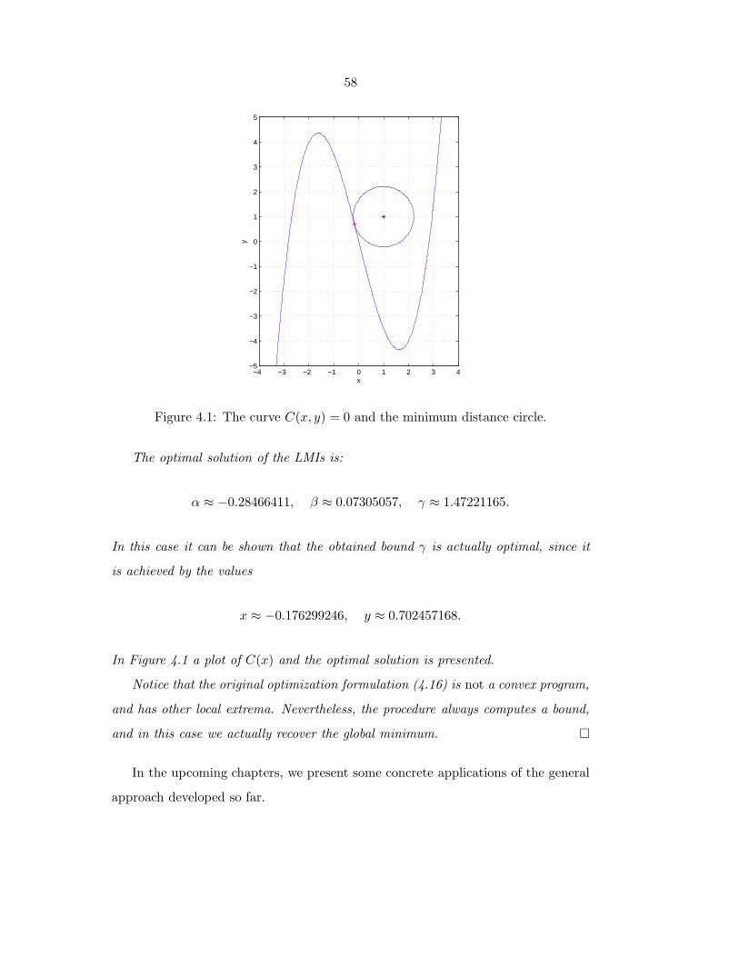
58
−4 −3 −2 −1 0 1 2 3 4−5
−4
−3
−2
−1
0
1
2
3
4
5
x
y
Figure 4.1: The curve C(x, y) = 0 and the minimum distance circle.
The optimal solution of the LMIs is:
α ≈ −0.28466411, β ≈ 0.07305057, γ ≈ 1.47221165.
In this case it can be shown that the obtained bound γ is actually optimal, since it
is achieved by the values
x ≈ −0.176299246, y ≈ 0.702457168.
In Figure 4.1 a plot of C(x) and the optimal solution is presented.
Notice that the original optimization formulation (4.16) is not a convex program,
and has other local extrema. Nevertheless, the procedure always computes a bound,
and in this case we actually recover the global minimum.
In the upcoming chapters, we present some concrete applications of the general
approach developed so far.
59
Chapter 5
Copositive matrices
The verification of matrix copositivity is a well-known computationally hard prob-
lem, with many applications in continuous and combinatorial optimization. In this
chapter, we present a hierarchy of semidefinite programming based sufficient con-
ditions for a real matrix to be copositive. These conditions are obtained through
the use of the sum of squares decomposition for multivariable forms, presented in
Chapter 4. As can be expected, there is a tradeoff between conservativeness of the
tests and the corresponding computational requirements. The proposed tests will
be shown to be exact for a certain family of extreme copositive matrices.
5.1 Copositivity
A real matrix M is said to be copositive if the quadratic form xTMx takes only
positive values in the nonnegative orthant (except the origin). Without loss of
generality, we can take M to be symmetric. As opposed to positive definiteness,
which can be efficiently verified (for example, using Gaussian elimination), there
seems to be no polynomial time algorithms for checking copositiveness.
Copositive matrices have numerous applications in diverse fields of applied math-
ematics, especially in optimization. It is a critical ingredient in the characterization
of local solutions of constrained optimization problems [65], such as the linear com-
plementarity problem [25]. Also, it has been recently shown that its use can notably
improve certain convex relaxation bounds in quadratic programming problems with

60
linear constraints [75]. As we have seen in the past chapters, these convex relax-
ations are the underlying basis of many important results in robustness analysis. A
recent example of an application of copositive matrices in a control setting is in the
stability analysis using piecewise quadratic Lyapunov functions [48].
From a computational complexity viewpoint, the recognition problem for coposi-
tive matrices is hard, in general. It has been shown that checking if a given matrix is
not copositive is an NP-complete problem [65]. Equivalently, checking copositivity
is in co-NPC (see [36, 70] for background material on computational complexity).
This implies that, unless co-NP=NP (a consequence of P=NP), in general it is not
possible to construct polynomial time certificates of copositivity (i.e., copositivity
is not in NP).
In many cases, however, it is possible to efficiently construct such certificates.
For example, assume that the matrix M has a decomposition M = P + N , with
P positive semidefinite and N componentwise nonnegative. It is clear that this
implies that M is copositive, with the matrices P and N providing a polynomial
time verifiable certificate.
In a similar way, the results presented in this chapter provide a unified method-
ology of constructing sufficient conditions for copositivity. The procedure uses as
a basic tool a sum of squares decomposition for multivariable forms, that can be
obtained by semidefinite programming methods, as we have seen before. As in the
other examples analyzed, one of the main advantages of the proposed procedure is
that it can also be applied to the case when the coefficients of M are variable (or
uncertain).
5.2 Background and notation
The notation is mostly standard. A matrix M ∈ Rn×n is copositive if xTMx ≥
0 ∀x ∈ Rn, xi ≥ 0. Equivalently, the quadratic form is nonnegative on the closed
nonnegative orthant. If xTMx takes only positive values on the closed orthant
(except the origin, of course), then M will be strictly copositive.
61
Recall the definition of geometric cones in page 11 of Chapter 2. A point x
of a convex cone C is an extreme point if x = x1 + x2, xi ∈ C implies x1 = λx,
x2 = (1 − λ)x, 0 ≤ λ ≤ 1. It can be shown that the set of copositive matrices C
is a closed convex cone [39]. We also denote as P,N the self-dual cones of positive
semidefinite and elementwise nonnegative matrices, respectively.
As in Chapter 4, denote by Fn,m the set of homogeneous polynomials (forms)
of degree m in n variables x1, . . . , xn, with real coefficients. Every such form can
be written as a sum of(n+m−1
m
)monomials, each one of the form cα
∏ni=1 x
αii , with∑n
i=1 αi = m.
There exist in the literature explicit necessary and sufficient conditions for a
given matrix to be copositive. These conditions are usually expressed in terms of
principal minors (see [90, 25] and the references therein). However, since checking
copositivity of a matrix is a co-NP-complete problem [65], this implies that in the
worst case these tests can take an exponential number of operations (unless P =
NP). Thus, the need for efficient sufficient conditions to guarantee copositivity.
We describe next two applications of copositive matrices, mentioned in the in-
troduction. Consider first the problem of obtaining a lower bound on the optimal
solution of a linearly constrained quadratic optimization problem [75].
Theorem 5.1 Let f∗ be the solution of the constrained minimization problem:
f∗ := minAx≥0, xTx=1
xTQx.
If the linear matrix inequality in C, γ:
Q−ATCA ≥ γI, (5.1)
is feasible, with a copositive C, then the inequality f∗ ≥ γ holds.
Proof: Multiply (5.1) left and right by any feasible x of the original problem. Since
Ax is componentwise nonnegative and C is copositive, we obtain xTQx ≥ γ.
62
A difficulty in the direct application of Theorem 5.1 is the fact that the set of
copositive matrices, though convex, does not have a “nice” description, since even
the problem of checking membership is provably hard. For this reason, having
semidefinite programming conditions that guarantee copositivity would allow for
enhanced bounds for this type of problems.
The other application, presented in [48, 49], deals with the analysis of piecewise
linear systems using piecewise quadratic Lyapunov functions. One of the basic issues
in that problem is checking nonnegativity of the Lyapunov function, in a region (or
“cell”) defined by linear inequalities. To this end, an LMI-based condition sufficient
condition is usually employed. By using the improved copositivity tests presented
in this paper, less conservative answers can be obtained, especially in the case of
systems of large state dimension. The conditions in [48] basically correspond to the
sufficient condition (5.3) below.
5.3 SDP conditions
In order to apply the sum of squares decomposition to the matrix copositivity prob-
lem, we need a way of dealing with the constraints in the variables, since each xi
has to be nonnegative. While we could directly impose the conditions xi ≥ 0 and
deal with them in the standard way suggested by the Positivstellensatz, we choose
here a perhaps more natural, though equivalent, procedure.
The alternative way of addressing the positivity constraint on the x variables is
the following: to check copositivity of M , we can consider the change of variables
xi = z2i , and study the global nonnegativity of the fourth order form given by:
P (z) := zTMz =∑i,j
mijz2i z
2j
where z = [z21 , z
22 , . . . , z
2n]T . It is easy to verify that M is copositive if and only if
the form P (z) is positive semidefinite. Therefore, an obvious sufficient condition for
M to be copositive is that P (z) can be written as a sum of squares.
In order to do that, as explained in previous chapters, we have to express P (z) as
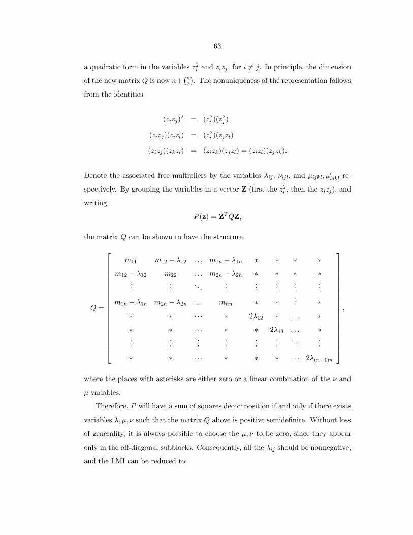
63
a quadratic form in the variables z2i and zizj , for i 6= j. In principle, the dimension
of the new matrix Q is now n+(n
2
). The nonuniqueness of the representation follows
from the identities
(zizj)2 = (z2i )(z2
j )
(zizj)(zizl) = (z2i )(zjzl)
(zizj)(zkzl) = (zizk)(zjzl) = (zizl)(zjzk).
Denote the associated free multipliers by the variables λij, νijl, and µijkl, µ′ijkl re-
spectively. By grouping the variables in a vector Z (first the z2i , then the zizj), and
writing
P (z) = ZTQZ,
the matrix Q can be shown to have the structure
Q =
m11 m12 − λ12 . . . m1n − λ1n ∗ ∗ ∗ ∗
m12 − λ12 m22 . . . m2n − λ2n ∗ ∗ ∗ ∗...
.... . .
......
......
...
m1n − λ1n m2n − λ2n . . . mnn ∗ ∗... ∗
∗ ∗ · · · ∗ 2λ12 ∗ . . . ∗
∗ ∗ · · · ∗ ∗ 2λ13 . . . ∗...
......
......
.... . .
...
∗ ∗ · · · ∗ ∗ ∗ · · · 2λ(n−1)n
,
where the places with asterisks are either zero or a linear combination of the ν and
µ variables.
Therefore, P will have a sum of squares decomposition if and only if there exists
variables λ, µ, ν such that the matrix Q above is positive semidefinite. Without loss
of generality, it is always possible to choose the µ, ν to be zero, since they appear
only in the off-diagonal subblocks. Consequently, all the λij should be nonnegative,
and the LMI can be reduced to:
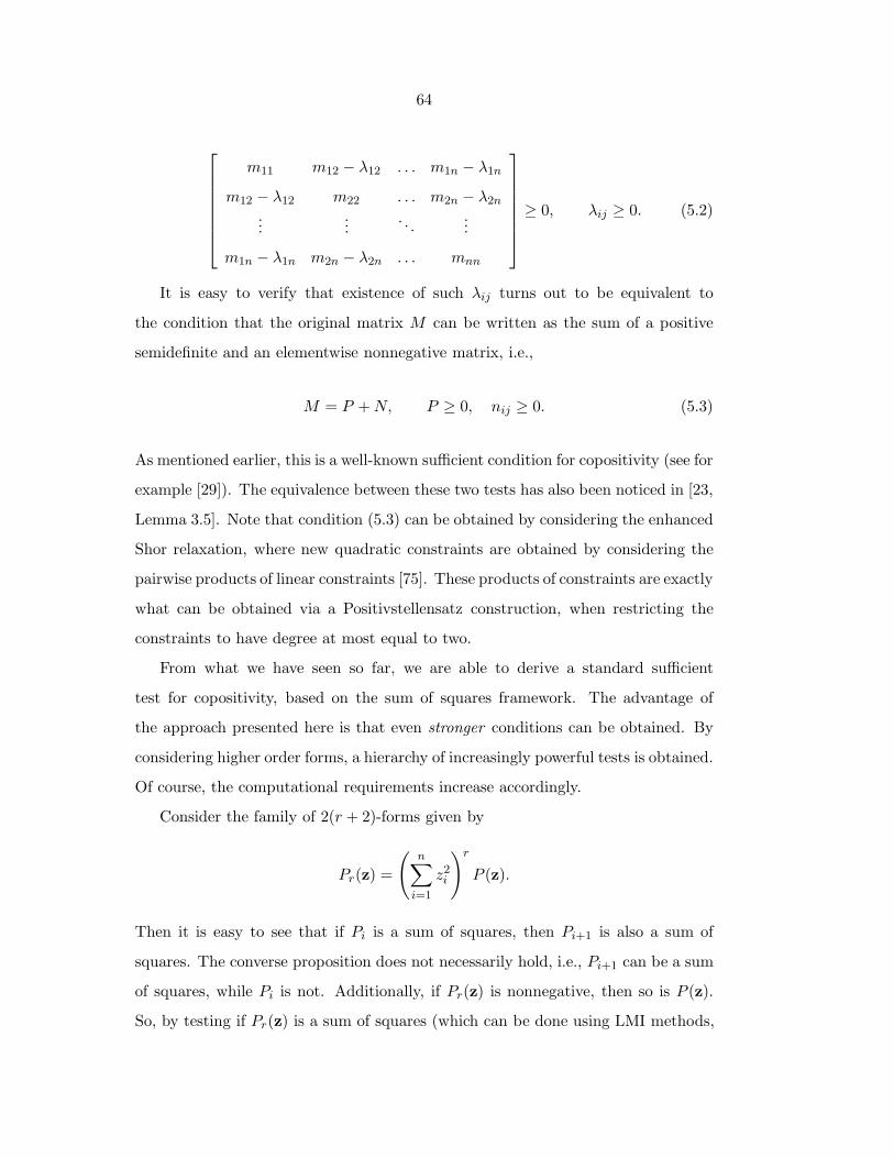
64
m11 m12 − λ12 . . . m1n − λ1n
m12 − λ12 m22 . . . m2n − λ2n...
.... . .
...
m1n − λ1n m2n − λ2n . . . mnn
≥ 0, λij ≥ 0. (5.2)
It is easy to verify that existence of such λij turns out to be equivalent to
the condition that the original matrix M can be written as the sum of a positive
semidefinite and an elementwise nonnegative matrix, i.e.,
M = P +N, P ≥ 0, nij ≥ 0. (5.3)
As mentioned earlier, this is a well-known sufficient condition for copositivity (see for
example [29]). The equivalence between these two tests has also been noticed in [23,
Lemma 3.5]. Note that condition (5.3) can be obtained by considering the enhanced
Shor relaxation, where new quadratic constraints are obtained by considering the
pairwise products of linear constraints [75]. These products of constraints are exactly
what can be obtained via a Positivstellensatz construction, when restricting the
constraints to have degree at most equal to two.
From what we have seen so far, we are able to derive a standard sufficient
test for copositivity, based on the sum of squares framework. The advantage of
the approach presented here is that even stronger conditions can be obtained. By
considering higher order forms, a hierarchy of increasingly powerful tests is obtained.
Of course, the computational requirements increase accordingly.
Consider the family of 2(r + 2)-forms given by
Pr(z) =
(n∑i=1
z2i
)rP (z).
Then it is easy to see that if Pi is a sum of squares, then Pi+1 is also a sum of
squares. The converse proposition does not necessarily hold, i.e., Pi+1 can be a sum
of squares, while Pi is not. Additionally, if Pr(z) is nonnegative, then so is P (z).
So, by testing if Pr(z) is a sum of squares (which can be done using LMI methods,
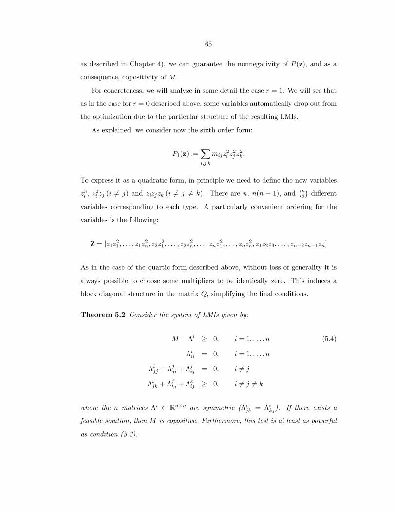
65
as described in Chapter 4), we can guarantee the nonnegativity of P (z), and as a
consequence, copositivity of M .
For concreteness, we will analyze in some detail the case r = 1. We will see that
as in the case for r = 0 described above, some variables automatically drop out from
the optimization due to the particular structure of the resulting LMIs.
As explained, we consider now the sixth order form:
P1(z) :=∑i,j,k
mijz2i z
2j z
2k.
To express it as a quadratic form, in principle we need to define the new variables
z3i , z2
i zj (i 6= j) and zizjzk (i 6= j 6= k). There are n, n(n − 1), and(n
3
)different
variables corresponding to each type. A particularly convenient ordering for the
variables is the following:
Z = [z1z21 , . . . , z1z
2n, z2z
21, . . . , z2z
2n, . . . , znz
21, . . . , znz
2n, z1z2z3, . . . , zn−2zn−1zn]
As in the case of the quartic form described above, without loss of generality it is
always possible to choose some multipliers to be identically zero. This induces a
block diagonal structure in the matrix Q, simplifying the final conditions.
Theorem 5.2 Consider the system of LMIs given by:
M − Λi ≥ 0, i = 1, . . . , n (5.4)
Λiii = 0, i = 1, . . . , n
Λijj + Λjji + Λjij = 0, i 6= j
Λijk + Λjki + Λkij ≥ 0, i 6= j 6= k
where the n matrices Λi ∈ Rn×n are symmetric (Λijk = Λikj). If there exists a
feasible solution, then M is copositive. Furthermore, this test is at least as powerful
as condition (5.3).

66
Proof: The nonnegativity of P1(z) follows immediately from the LMIs above, since
∑j,k
mjkxjxk ≥∑j,k
Λijkxjxk =⇒∑i,j,k
mjkxixjxk ≥∑i,j,k
Λijkxixjxk,
and the coefficients of this last form are nonnegative.
It is also possible to verify directly that if the LMIs (5.2) have a solution, then
so does the system (5.4). Just let
Λkij = λij(1− δik − δjk)
where δ is the usual Kronecker symbol, and λii = 0 for all i. This is a
consequence of the “nested” properties of the Pr-based tests.
As we have shown, this class of tests is at least as powerful as the standard
condition (5.3). A question naturally arises: how conservative is this procedure? To
this end, consider the following theorem of Polya:
Theorem 5.3 [40, Section 2.24] Given a form F (x1, x2, . . . , xn) strictly positive
for xi ≥ 0,∑
i xi > 0, then F can be expressed as
F =G
H,
where G and H are forms with positive coefficients. In particular, we can choose
H = (x1 + x2 + · · ·+ xn)r
for a suitable r.
Applying the theorem to a strictly copositive M (i.e., to the associated positive
definite form P (z)), it is clear then that there is a finite r for which the condition
based on Pr is exact. However, the minimum r in Theorem 5.3 cannot always
be chosen as a polynomial expression of n (uniformly over the psd forms). The
known lower bounds for r usually involve a “condition number” for the form P :
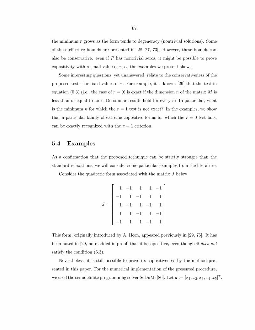
67
the minimum r grows as the form tends to degeneracy (nontrivial solutions). Some
of these effective bounds are presented in [28, 27, 73]. However, these bounds can
also be conservative: even if P has nontrivial zeros, it might be possible to prove
copositivity with a small value of r, as the examples we present shows.
Some interesting questions, yet unanswered, relate to the conservativeness of the
proposed tests, for fixed values of r. For example, it is known [29] that the test in
equation (5.3) (i.e., the case of r = 0) is exact if the dimension n of the matrix M is
less than or equal to four. Do similar results hold for every r? In particular, what
is the minimum n for which the r = 1 test is not exact? In the examples, we show
that a particular family of extreme copositive forms for which the r = 0 test fails,
can be exactly recognized with the r = 1 criterion.
5.4 Examples
As a confirmation that the proposed technique can be strictly stronger than the
standard relaxations, we will consider some particular examples from the literature.
Consider the quadratic form associated with the matrix J below.
J =
1 −1 1 1 −1
−1 1 −1 1 1
1 −1 1 −1 1
1 1 −1 1 −1
−1 1 1 −1 1
This form, originally introduced by A. Horn, appeared previously in [29, 75]. It has
been noted in [29, note added in proof] that it is copositive, even though it does not
satisfy the condition (5.3).
Nevertheless, it is still possible to prove its copositiveness by the method pre-
sented in this paper. For the numerical implementation of the presented procedure,
we used the semidefinite programming solver SeDuMi [86]. Let x := [x1, x2, x3, x4, x5]T .

68
Taking r = 1, after solving the corresponding LMIs we obtain the decomposition:
(xTJx) (x1 + x2 + x3 + x4 + x5) = x1(x1 − x2 + x3 + x4 − x5)2 +
x2(x2 − x3 + x4 + x5 − x1)2 +
x3(x3 − x4 + x5 + x1 − x2)2 +
x4(x4 − x5 + x1 + x2 − x3)2 +
x5(x5 − x1 + x2 + x3 − x4)2 +
4 (x1x2x4 + x2x3x5 + x3x4x1 + x4x5x2 + x5x1x3)
from where copositivity of J follows immediately.
This example can be generalized to a family of copositive forms, with interesting
theoretical properties. Consider the following cyclic quadratic form in n = 3m + 2
variables (m ≥ 1), analyzed in [6]:
B(x) :=
(3m+2∑i=1
xi
)2
− 23m+2∑i=1
xi
m∑j=0
xi+3j+1 (5.5)
where xr+n = xr. It is clear that the Horn form presented above corresponds to the
special case m = 1. It has been shown in [6] that this is a extreme copositive form.
Therefore, since B(x) is neither componentwise nonnegative or positive semidefinite,
it cannot satisfy condition (5.3). Generalizing the decomposition above, we have the
following theorem:
Theorem 5.4 Let B(x) be as in equation (5.5). Then, it has the decomposition:
B(x)n∑i=1
xi =n∑i=1
xi
n∑j=1
xj − 2m∑j=0
xi+3j+1
2
+ 4n∑i=1
xi
m∑k=1
xi+3k−2
m∑j=k
xi+3j
(5.6)
Proof: For notational simplicity, let si(x) := xi+1 +xi+4 + · · ·+xi+3m+1. Let L(x)

69
be the left-hand side of (5.6). Then,
L(x) =n∑i=1
n∑j=1
n∑k=1
xixjxk − 2n∑i=1
n∑k=1
xixksi(x)
The first term in the right-hand size of (5.6) can be written as:
R1(x) =n∑i=1
xi
n∑j=1
xj − 2si(x)
2
=n∑i=1
n∑j=1
n∑k=1
xixjxk − 4n∑i=1
n∑j=1
xixjsi(x) + 4n∑i=1
xis2i (x)2
Subtracting, we obtain:
L(x)−R1(x) = 2n∑i=1
n∑j=1
xixjsi(x)− 4n∑i=1
xis2i (x)2
= 2n∑i=1
xi
n∑j=1
xj − 2si(x)
si(x)
Expanding inside the sum, and cancelling identical terms corresponding to
different values of i, after some manipulations we obtain the expression:
R1(x) = 4n∑i=1
xi
m∑k=1
xi+3k−2(xi+3k + xi+3(k+1) + · · ·+ xi+3m),
from where the result follows.

70

71
Chapter 6
Higher order semidefinite relaxations
In this chapter, we specialize the general machinery presented earlier in order to
formulate improved versions of the standard semidefinite relaxation for quadratic
programming. This framework underlies many important results in robustness anal-
ysis and combinatorial optimization. It is shown that the proposed polynomial time
convex conditions are at least as strong as the standard case, and usually better,
but at a higher computational cost. Several applications of the new relaxations are
provided, including less conservative upper bounds for the structured singular value
µ, and enhanced solutions for the MAX CUT graph partitioning problem.
6.1 Introduction
Many problems in systems and control theory, especially in robustness analysis
and synthesis, have intrinsically “bad” computational complexity properties. As
mentioned in the introduction, these features (for example, being NP-hard) are
specific to the problem class, and not associated with any particular algorithm used
in its solution. In the case of NP-hardness, in particular, the practical implications
are well known: unless P=NP, every algorithm that solves the problem will take at
least an exponential number of steps, in the worst case.
For this reason, it is particularly useful to count with alternative methods, guar-
anteed to run in a “reasonable” time, that provide bounds on the optimal solution
and/or suboptimal estimates. In the particular case of quadratic programming
72
(QP), such a tool has been made available in the last few years. Semidefinite pro-
gramming (SDP) relaxations of nonconvex QP problems are increasingly being used
for a variety of problems in diverse fields of applied mathematics. These SDP re-
laxations are convex optimization problems, that can be solved in polynomial time.
The procedure by which we obtain a relaxed problem and its dual is known in the
literature under several different names, i.e., S-procedure, Shor relaxation, covari-
ance relaxation, lifting, etc. [91]. For certain specific cases (such as the MAX CUT
problem discussed below) these approximate solutions are provably good, as there
exist hard bounds on their degree of suboptimality. However, some other problems
(for instance, MAX CLIQUE, or real µ [32]) are significantly harder, since even the
approximation problem within an arbitrary constant factor is NP-hard.
In this chapter, we present a novel convex relaxation of quadratic programming
problems, that runs in polynomial time. The idea can be interpreted as finding a
separating functional (not necessarily linear) that proves that the intersection of two
sets is empty. As in the previous chapter, we employ as a basic technique the exis-
tence of a sum of squares decomposition as a sufficient condition for nonnegativity
of a multivariable form.
6.2 The standard SDP relaxation
The viewpoint taken here focuses on considering the standard SDP relaxation as
a sufficient condition for establishing that a certain set A (described by strict
quadratic inequalities) is empty. Concretely, given m symmetric matrices A1, . . . , Am ∈
Rn×n, the set A is given by the intersection of the image of Rn under the quadratic
forms and the positive orthant, i.e.:
A :=z ∈ Rm| zi ≥ 0, zi = xTAix, x ∈ Rn/0, i = 1, . . . ,m
(6.1)
For future reference, let a(x) := [xTA1x, . . . ,xTAmx]T . Both logical implications
and constrained optimization problems can be put in the form (6.1), by checking
for the existence of a counterexample, or a feasible point that achieves a given level
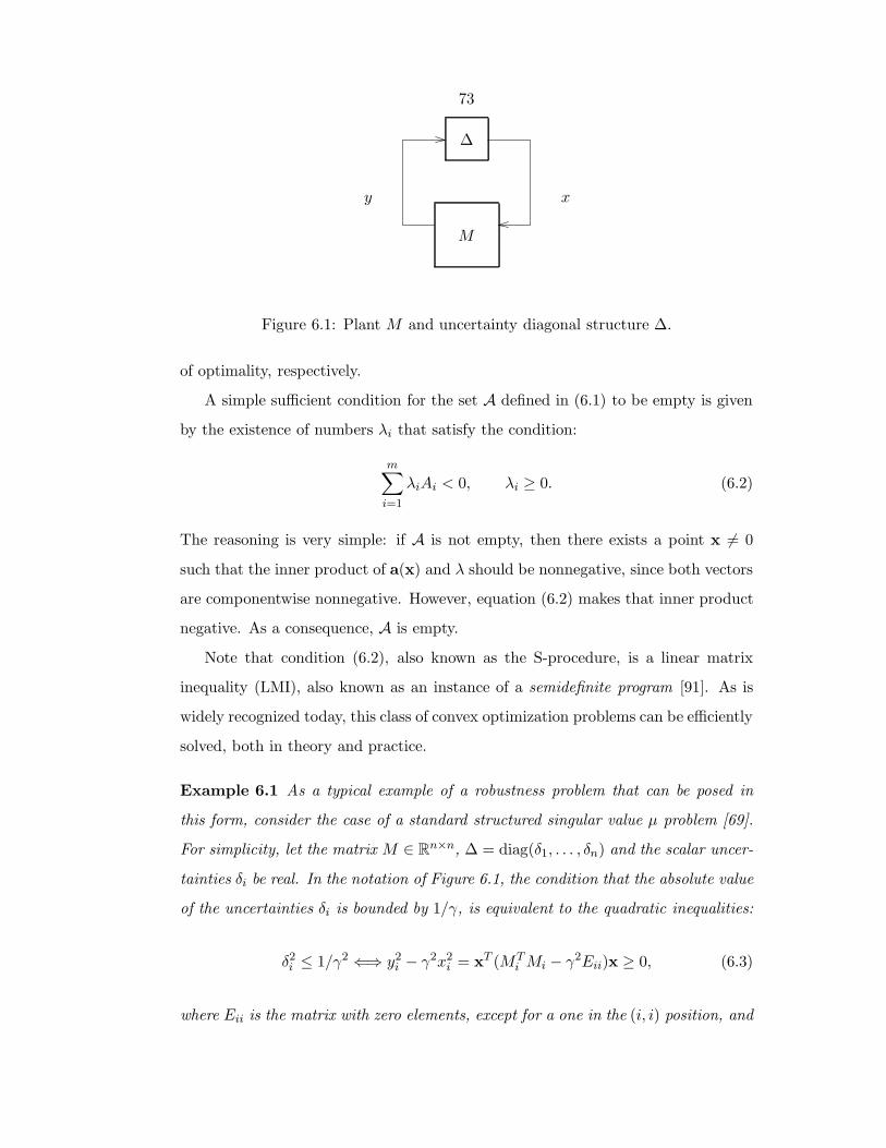
73
∆
M
xy
Figure 6.1: Plant M and uncertainty diagonal structure ∆.
of optimality, respectively.
A simple sufficient condition for the set A defined in (6.1) to be empty is given
by the existence of numbers λi that satisfy the condition:
m∑i=1
λiAi < 0, λi ≥ 0. (6.2)
The reasoning is very simple: if A is not empty, then there exists a point x 6= 0
such that the inner product of a(x) and λ should be nonnegative, since both vectors
are componentwise nonnegative. However, equation (6.2) makes that inner product
negative. As a consequence, A is empty.
Note that condition (6.2), also known as the S-procedure, is a linear matrix
inequality (LMI), also known as an instance of a semidefinite program [91]. As is
widely recognized today, this class of convex optimization problems can be efficiently
solved, both in theory and practice.
Example 6.1 As a typical example of a robustness problem that can be posed in
this form, consider the case of a standard structured singular value µ problem [69].
For simplicity, let the matrix M ∈ Rn×n, ∆ = diag(δ1, . . . , δn) and the scalar uncer-
tainties δi be real. In the notation of Figure 6.1, the condition that the absolute value
of the uncertainties δi is bounded by 1/γ, is equivalent to the quadratic inequalities:
δ2i ≤ 1/γ2 ⇐⇒ y2
i − γ2x2i = xT (MT
i Mi − γ2Eii)x ≥ 0, (6.3)
where Eii is the matrix with zero elements, except for a one in the (i, i) position, and

74
Mi is the ith row of the matrix M . Therefore, for this particular case, the matrices
Ai are given by Ai = MTi Mi − γ2Eii. In this case, the nonexistence of nontrivial
solutions can be interpreted as the robust stability of the system under uncertainty.
When we apply the SDP relaxation to the system of inequalities (6.3), we obtain
the usual µ upper bound LMI, with D being a diagonal matrix:
MTDM − γ2D < 0, D > 0. (6.4)
It is also interesting to study the dual problem of (6.2). It consists of checking for
the existence of a symmetric matrix Z 6= 0, that satisfies
traceAiZ ≥ 0, Z ≥ 0. (6.5)
This dual problem can also be obtained directly from (6.1), by using the cyclic
properties of the trace function, and dropping the rank one condition on the matrix
Z := xxT [91]. If this dual problem does not have a solution, then neither does
the original one. But at least in principle, an affirmative answer to the feasibility of
(6.5) does not necessarily say anything about the set A (in some special cases, it is
possible to extract useful information from the matrix Z).
6.3 Separating functionals and a new SDP relaxation
In order to extend the standard condition, we will be considering the well-known
interpretation of the multipliers λi in (6.2) as defining a separating hyperplane (or
a linear functional). To see this, notice that the positivity condition on the multi-
pliers λi guarantees that the linear functional φ(z) = λT z is positive in the positive
orthant. Additionally, condition (6.2) ensures that this functional is negative on the
image of Rn under the map a. Therefore, those two sets have empty intersection,
which is what we want to prove.
Understanding this idea, the proposed method is conceptually simple: replace
75
the linear form by a more general function. For consistency with the linear case,
we keep using the term “functional” to refer to these mappings; see for example
[54, Section 13.5]. For concreteness, we will consider only the case of quadratic
functionals, though the extension to the general case is straightforward. The reasons
are also practical: the complexity of checking nonnegativity of forms of high degree
grows quite fast. Even in the relatively simple case of quartic forms (as in the case
we will be analyzing), the computation requirements can be demanding.
Extending the definitions from the previous chapter, a functional φ : Rn → R is
copositive if xi ≥ 0 implies φ(x) ≥ 0, i.e., is positive in the positive orthant. In this
case, it is clear that a sufficient condition for A being empty is the existence of a
copositive functional φ such that:
φ(a(x)) < 0, ∀x ∈ Rn/0 (6.6)
The reasons are exactly as above: the existence of a possible x that makes a(x)
nonnegative forces the composition of the functions to be positive or zero, contra-
dicting the condition above. Note that the same conclusions hold if φ itself depends
on x, as long as it is always copositive.
Two questions immediately arise: How do we characterize copositive functionals,
and how do we check condition (6.6)? From a complexity viewpoint, these two
questions are as intractable as the original problem. It turns out that for the case
of polynomial functionals φ, a partial answer to both questions can be obtained by
using the sum of squares decomposition presented in Chapter 4.
For the exact copositivity problem, the results mentioned in the previous chapter
show that checking if a quadratic form is not copositive is an NP-complete problem
[65]. As we have seen, a simple sufficient condition for copositivity of a matrix Φ
(see Chapter 5 for stronger SDP-based copositivity tests) is given by the existence
of a decomposition of Φ as the sum of two matrices, one positive definite and the
other one componentwise nonnegative, i.e.:
Φ = P +N, P ≥ 0, nij ≥ 0.
76
Notice that without loss of generality, we can always take the diagonal elements of
N to be zero.
Therefore, we can consider quadratic copositive functionals φ of the form above
(i.e. φ(v) := vTΦxv), applied to the vector [1,a(x)]T , since we want to allow for
linear terms too. For reasons that will be clear later, we would like the LHS of (6.6)
to be a homogeneous form. This imposes certain constraints in the structure of φ.
It can be verified that the positive definite part of φ cannot help in making the form
negative definite. Based on all these facts, a sufficient condition for A being empty
is presented next, where we also consider the case of equality constraints.
Theorem 6.1 Assume there exists solutions Qi, Ti ∈ Rn×n, rij ∈ R to the equation
na∑i=1
Qi(x)Ai(x) +∑
1≤i<j≤narijAi(x)Aj(x) +
nb∑j=1
Tj(x)Bj(x) < 0, ∀x ∈ Rn/0.
(6.7)
where Qi(x) := xTQix, Tj(x) := xTTjx,Qi ≥ 0 and rij ≥ 0. Then, the only solution
of
Ai(x) ≥ 0, i = 1, . . . , na
Bi(x) = 0, i = 1, . . . , nb
is x = 0.
Proof: It basically follows from the same arguments as in the linear case: the exis-
tence of a nontrivial x implies a contradiction. Therefore, the set A is neces-
sarily empty.
Note that the left-hand size of the equation above is a homogeneous form of degree
four. Checking the full condition as written would be again a hard problem, so we
check instead a sufficient condition: that the LHS of (6.7) can be written (except
for the sign change) as a sum of squares. As we have seen before in Chapter 4, this
can be checked using semidefinite programming methods.
77
The new relaxation is always at least as powerful as the standard one: this can
be easily verified, just by taking Qi = λiI and rij = 0. Then, if (6.2) is feasible,
then the left-hand side of (6.7) is obviously a sum of squares (recall that positive
definite quadratic forms are always sums of squares).
Remark 6.1 It is interesting to compare this condition with the Nullstellensatz
and Positivstellensatz in Chapter 4. The first two terms in (6.7) belong to the cone
generated by the Ai(x), and the remaining one to the ideal corresponding to the
Bi(x). The degree of the multipliers is restricted, so the whole expression is an
homogeneous form of fixed degree.
It is often the case that one of the quadratic forms, say A1, depends on a certain
parameter γ, and we are interested in finding the smallest (or largest) value of γ
for which the set A(γ) is empty. In this case, when we take into account the γ
dependence of A1, the problem of testing feasibility of (6.7) is no longer an LMI,
since we have products of γ and the decision variables Qi and qij. There are two
possible remedies to this problem: the first one is to remember that even though
(6.7) is not a semidefinite program, it is still a quasiconvex problem, since for fixed γ
the level sets are convex. The alternative is to fix some of the variables (for example,
Q1 = I, and q1j = 1), to make the left-hand size of (6.7) linear in γ. In principle,
this last technique can be conservative, when comparing to the case where all the
variables are free.
6.3.1 Computational complexity
A few words on the complexity of the proposed procedure are in order. When solv-
ing the relaxation using standard software, the main burden lies in the computation
of the solution of the resulting system of LMIs, in particular due to the need of
checking if the resulting quartic form is a sum of squares. The LMI correspond-
ing to this condition has dimensions(n+1
2
). However, the main difficulty is really
caused by the large number of variables, since the ones arising from the redundant
constraints, as explained before, are O(n4). Even though it is polynomial (and
78
therefore the whole procedure runs in polynomial time), this rapid growth rate is
not quite acceptable. In many special cases, symmetry considerations can help re-
duce the number significantly. However, for the general case with a large number of
variables, alternative approaches are certainly needed. Some concrete possibilities,
currently under study, are to exploit problem structure, and to incorporate only a
certain subset of variables into the optimization.
6.4 Relaxations and moments
In the case where the relaxation is not exact, we do not obtain a feasible point
in the primal problem, and end up only with lower bounds on the optimal value.
Naturally, we would also like to have some upper bounds, so it would be interesting
to have some approximate procedure or guidelines to construct a primal feasible
point. In this case, a sensible approach, very successful in some specific problems,
is a randomized procedure.
In the standard SDP relaxation, the dual variables can be interpreted as pro-
viding the matrix of second moments for a particular probability distribution. In
the case of the MAX CUT problem discussed in the examples below, for instance,
primal points can be constructed by randomly generating points consistent with
this probability density (given by the matrix Y ), and rounding them to the values
±1. In this specific case, good bounds can be obtained on the expected value of the
resulting cut [37].
In principle, in certain instances we can do so in our case too. However, there are
some important differences. In the quadratic case, any positive semidefinite matrix
is a valid candidate for a set of second moments; for example, we can construct
a multivariate normal distribution with that preassigned covariance. However, for
higher order moments, not every set of numbers obtained from the relaxation nec-
essarily correspond to the moments of a measure [1, 8]. The root of this problem,
it turns out, is again the distinction between the conditions of nonnegativity of a
polynomial and being a sum of squares.
79
A notable exception is the one dimensional case, since given a sequence of mo-
ments, positive semidefiniteness of the corresponding Hankel matrix is enough to
guarantee the existence of a measure with exactly those moments [1]. Interestingly
enough, this problem is very related to the Nevanlinna-Pick interpolation questions
studied in H∞ control.
6.5 Examples
In this section, we present a few applications of the new relaxations to some prac-
tically important problems.
6.5.1 Structured singular value upper bound
As mentioned in Example 6.1, the standard upper bound of the structured singular
value µ [69] can be interpreted as the result of applying the standard relaxation to
the quadratic forms defining the uncertainty structure. It is therefore a natural test
problem for the presented techniques.
Given a matrixM ∈ Cn×n, and an uncertainty structure ∆, define the structured
singular value µ as:
µ∆(M) :=1
min‖∆‖ : ∆ ∈∆,det(I −M∆) = 0 , (6.8)
unless no ∆ makes I −M∆ singular, in which case µ∆(M) := 0. An upper bound
for µ can be obtained by solving the LMI presented in Example 6.1.
We consider next the counterexample, due to Morton and Doyle, to the propo-
sition that µ equals to its standard upper bound in the case with four scalar uncer-
tainties [69, Section 9.2]. This corresponds to a certain rank two matrix M ∈ C4×4,

80
given by:
M := UV ∗, U =
a 0
b b
c jc
d f
, V =
0 a
b −b
c −jc
−jf −d
,
with a =√
2/γ, b = 1/√γ, c = 1/
√γ, d = −
√β/γ, f = (1 + j)
√1/γβ, γ = 3 +
√3,
and β =√
3− 1. This matrix has a value of µ ≈ 0.8723. However, the standard µ
upper bound, given by equation (6.4), has an exact value of 1. For this problem,
with the improved relaxation, we are able to prove an upper bound of 0.895 by
solving a semidefinite program.
6.5.2 The MAX CUT problem
The maximum cut (MAX CUT) problem consists in finding a partition of the nodes
of a graph in two disjoint sets V1 and V2, in such a way to maximize the number of
edges that have an endpoint in V1 and the other in V2. It has important practical
applications, such as optimal circuit layout. The decision version of this problem
(does there exist a cut with value greater than or equal to K?) is known to be
NP-complete [36].
By casting the problem as a boolean maximization, we can write the MAX CUT
problem as an equality constrained quadratic program. One standard formulation
is the following:
maxyi∈−1,1
12
∑i,j
wij(1− yiyj), (6.9)
where wij is the weight corresponding to the (i, j) edge, and is zero if the nodes i and
j are not connected. The constraints yi ∈ −1, 1 are equivalent to the quadratic
constraints y2i = 1.
We can obtain useful upper bounds on the optimal value of (6.9) using semidefi-
nite programming. Removing the constant term, and changing the sign, the original
81
problem is clearly equivalent to:
miny2i=1
∑i,j
wijyiyj. (6.10)
The corresponding semidefinite relaxation is given by:
minY≥0,Yii=1
traceWY, (6.11)
and its dual
maxD≤W
traceD, (6.12)
where D is a diagonal matrix. Any feasible solution of the dual (6.12) provides a
lower bound on the optimal value of (6.11), and therefore on that of (6.10).
It has been recently shown by Goemans and Williamson [37] that by randomly
truncating in an appropriate manner the solution Y of this relaxation, a cut with
an expected value greater than 87% of the optimal MAX CUT solution is obtained.
In this sense, for the MAX CUT problem the semidefinite relaxation is provably
“good.” Note however that for other NP-complete problems, such as MAX CLIQUE,
no such approximation results hold, unless P=NP.
The enhanced relaxations developed earlier in this chapter can be directly ap-
plied, by testing if the set of solutions yi of (6.9) that achieve a value greater than
or equal to γ is empty. Since the constraints defining the problem are quadratic,
this problem formulation corresponds exactly to the setting of Theorem 6.1. The
variable γ can be included in the optimization problem, as described in page 77.
A simple case where both the exact problem and the standard SDP relaxation
can be analyzed is that of the n-cycle Cn. This is a graph with n nodes and n edges,
where the edges form a closed chain. In other words, if the vertices are numbered
from v1 to vn, then all the edges have the form (vi, vi+1), where vn+1 = v1. For this
graph, the exact value for the unweighted MAX CUT problem can easily be shown
to be equal to n if n is even, or n− 1 otherwise.
In the case of even n, the standard relaxation provides a bound that is exact
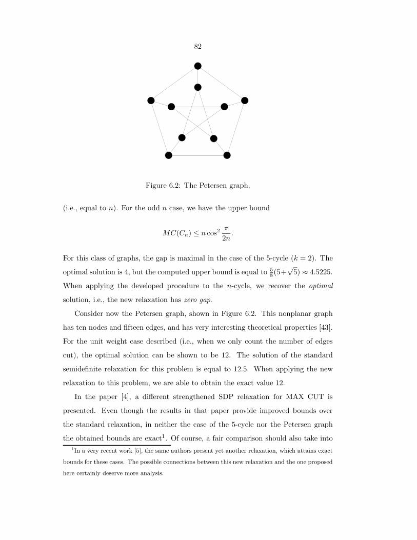
82
Figure 6.2: The Petersen graph.
(i.e., equal to n). For the odd n case, we have the upper bound
MC(Cn) ≤ n cos2 π
2n.
For this class of graphs, the gap is maximal in the case of the 5-cycle (k = 2). The
optimal solution is 4, but the computed upper bound is equal to 58(5+
√5) ≈ 4.5225.
When applying the developed procedure to the n-cycle, we recover the optimal
solution, i.e., the new relaxation has zero gap.
Consider now the Petersen graph, shown in Figure 6.2. This nonplanar graph
has ten nodes and fifteen edges, and has very interesting theoretical properties [43].
For the unit weight case described (i.e., when we only count the number of edges
cut), the optimal solution can be shown to be 12. The solution of the standard
semidefinite relaxation for this problem is equal to 12.5. When applying the new
relaxation to this problem, we are able to obtain the exact value 12.
In the paper [4], a different strengthened SDP relaxation for MAX CUT is
presented. Even though the results in that paper provide improved bounds over
the standard relaxation, in neither the case of the 5-cycle nor the Petersen graph
the obtained bounds are exact1. Of course, a fair comparison should also take into1In a very recent work [5], the same authors present yet another relaxation, which attains exact
bounds for these cases. The possible connections between this new relaxation and the one proposed
here certainly deserve more analysis.
83
account the computational requirements, which are higher in our proposed method
than in that of [4]. We also note that a usual technique to decrease the possible
conservativeness of the MAX CUT relaxation is to add linear odd cycle constraints.
The complexity of doing this (for the three point case) is lower than the one of our
proposed relaxation. For this case, in the small problems we have tested, the results
seem to be equivalent. However, more numerical experience and theoretical insight
is needed in order to formulate accurate comparisons.
6.6 Final overview
A new polynomial time scheme for computing bounds on the optimal solution of hard
nonconvex problems was introduced. The resulting estimates are always at least as
strong as the ones obtained by the traditional semidefinite relaxation. The key idea
is to use a sum of squares decomposition as a sufficient condition for nonnegativity
of a function. The results obtained from its application to a few test problems are
certainly encouraging: tighter (or even exact) bounds can be obtained. Of course,
more study is needed in order to fully assess its potential relevance, especially in
terms of practical performance.

84

85
Chapter 7
Applications in systems and control
In this chapter, we show how the methods developed in the preceding sections can be
profitably applied to systems and control related problems. Some of the presented
applications correspond to well-studied problems, such as Lyapunov function com-
putation, while others, such as robust bifurcation analysis, are relatively new.
The main insight underlying the results in this chapter is that under certain
assumptions, many conditions (for example, existence of a Lyapunov function) can
be equivalently formulated in terms of polynomial equalities and inequalities. In
other words, the set of feasible parameters is a semialgebraic set. In this case,
operations such as testing for emptyness, obtaining bounds on the distance to a
given point, etc., can all be formulated and solved within the framework described
in Chapter 4. The main advantages are the resulting computational tractability
(since it reduces to semidefinite programs), as well as the algorithmic character of
the solution procedure.
As an motivating example of the methodology, we will deal in the next section
mainly with the stability analysis of systems described by polynomial vector fields.
Later we will show that the same techniques can be employed to more complicated
problems.
86
7.1 Lyapunov stability
Stability analysis can be reduced, using Lyapunov theory, to the existence of a
positive definite function, such that its time derivative along the trajectories of the
system is negative. As is well known, to prove asymptotic stability of a fixed point of
vector field (the origin, without loss of generality) it is required to find a Lyapunov
function V (x) such that:
x = f(x), V (x) > 0 x 6= 0,
V (x) =(∂V
∂x
)Tf(x) < 0, x 6= 0 (7.1)
for all x in a neighborhood of the origin. If we want global results, we need additional
conditions such as V being radially unbounded.
In the specific case of linear systems x = Ax and quadratic Lyapunov functions
V (x) = xTPx, this stability test is equivalent to the well-known LMIs
ATP + PA < 0, P > 0.
The existence of a P satisfying this last condition can be checked efficiently, using
for instance interior point methods.
For nonlinear systems, in the general case there are no systematic methodologies
for the search for Lyapunov functions [51]. Nevertheless, in the presence of addi-
tional structure, such as the case of mechanical systems, sometimes it is possible to
find natural energy-based Lyapunov functions. Alternative approaches use an em-
bedding (overbounding) of the given nonlinear system in a class of uncertain linear
systems. This is the case, to cite a few, of conic sector bounds, Linear Parameter
Varying (LPV) and Integral Quadratic Constraints (IQC, [61]) based methods. The
methology presented in this section, on the contrary, handles polynomial nonlinear-
ities exactly.
In the attempt to extend the algorithmic formulation to more general vector
fields (not necessarily linear) or Lyapunov functions (not necessarily quadratic),
87
we are faced with the basic question of how to verify in a systematic fashion the
conditions (7.1). If we want to develop an algorithmic approach to nonlinear system
analysis, similar to what is available in the linear case, we need some explicit way
of testing the global positivity of a function. In the case of polynomial functions, a
tractable sufficient condition, as presented in Chapter 4, is the existence of a sum
of squares decomposition.
Example 7.1 The system below is from [13, Example 2.5]. Given the nonlinear
system
x1 = −x31 − x2x3 − x1 − x1x
23
x2 = −x1x3 + 2x31 − x2
x3 = −x3 + 2x21
and the (fixed) Lyapunov function V (x) = 12(x2
1 + x22 + x2
3), test if V (x) is negative
definite.
After computing V , we can test if we can express it as a sum of squares using
the methodology described. In this case, the decomposition
−V (x) = x21 + x2
3 + (x21 − x1x3 − x2)2
is obtained, from where global stability follows.
7.2 Searching for a Lyapunov function
Given an affine parametrization V (x, p) of the Lyapunov function, the search for a
Lyapunov function can be automated, since in this case the polynomial
−V (x, p) = −(∂V
∂x
)Tf(x)
is again affine in p. Therefore, by including the parameters p as variables in the
LMI, the full problem can be reformulated as a linear matrix inequality.
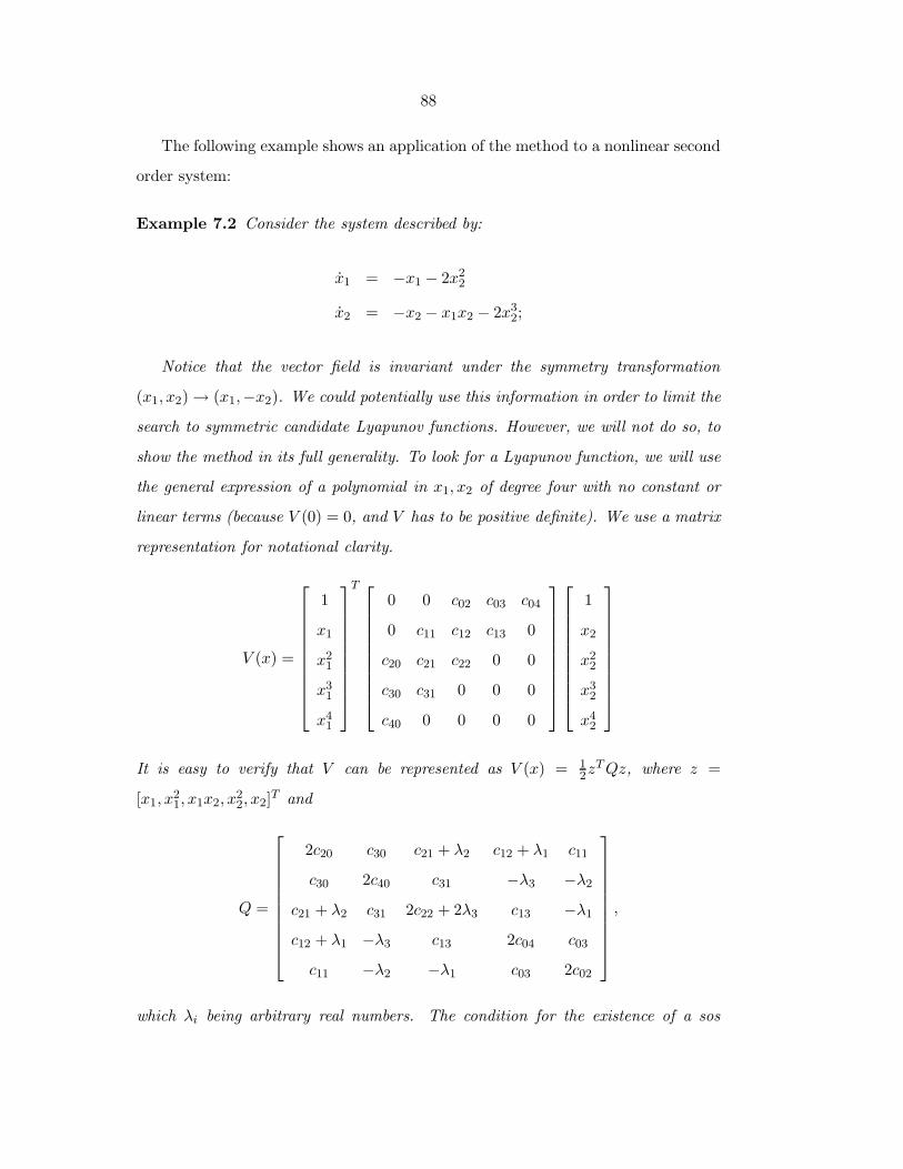
88
The following example shows an application of the method to a nonlinear second
order system:
Example 7.2 Consider the system described by:
x1 = −x1 − 2x22
x2 = −x2 − x1x2 − 2x32;
Notice that the vector field is invariant under the symmetry transformation
(x1, x2)→ (x1,−x2). We could potentially use this information in order to limit the
search to symmetric candidate Lyapunov functions. However, we will not do so, to
show the method in its full generality. To look for a Lyapunov function, we will use
the general expression of a polynomial in x1, x2 of degree four with no constant or
linear terms (because V (0) = 0, and V has to be positive definite). We use a matrix
representation for notational clarity.
V (x) =
1
x1
x21
x31
x41
T
0 0 c02 c03 c04
0 c11 c12 c13 0
c20 c21 c22 0 0
c30 c31 0 0 0
c40 0 0 0 0
1
x2
x22
x32
x42
It is easy to verify that V can be represented as V (x) = 1
2zTQz, where z =
[x1, x21, x1x2, x
22, x2]T and
Q =
2c20 c30 c21 + λ2 c12 + λ1 c11
c30 2c40 c31 −λ3 −λ2
c21 + λ2 c31 2c22 + 2λ3 c13 −λ1
c12 + λ1 −λ3 c13 2c04 c03
c11 −λ2 −λ1 c03 2c02
,
which λi being arbitrary real numbers. The condition for the existence of a sos
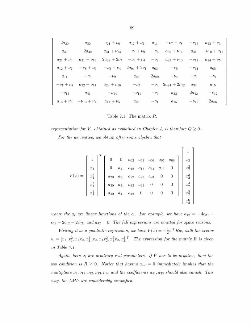
89
2a20 a30 a21 + ν6 a12 + ν2 a11 −ν7 + ν8 −ν13 a13 + ν3
a30 2a40 a31 + ν13 −ν8 + ν9 −ν6 a32 + ν14 a41 −ν10 + ν11
a21 + ν6 a31 + ν13 2a22 + 2ν7 −ν3 + ν4 −ν2 a23 + ν10 −ν14 a14 + ν5
a12 + ν2 −ν8 + ν9 −ν3 + ν4 2a04 + 2ν1 a03 −ν5 −ν11 a05
a11 −ν6 −ν2 a03 2a02 −ν4 −ν9 −ν1
−ν7 + ν8 a32 + ν14 a23 + ν10 −ν5 −ν4 2a24 + 2ν12 a33 a15
−ν13 a41 −ν14 −ν11 −ν9 a33 2a42 −ν12
a13 + ν3 −ν10 + ν11 a14 + ν5 a05 −ν1 a15 −ν12 2a06
Table 7.1: The matrix R.
representation for V , obtained as explained in Chapter 4, is therefore Q ≥ 0.
For the derivative, we obtain after some algebra that
V (x) =
1
x1
x21
x31
x41
T
0 0 a02 a03 a04 a05 a06
0 a11 a12 a13 a14 a15 0
a20 a21 a22 a23 a24 0 0
a30 a31 a32 a33 0 0 0
a40 a41 a42 0 0 0 0
1
x2
x22
x32
x42
x52
x62
where the ai are linear functions of the ci. For example, we have a12 = −4c20 −
c12 − 2c12 − 2c02, and a42 = 0. The full expressions are omitted for space reasons.
Writing it as a quadratic expression, we have V (x) = −12w
TRw, with the vector
w = [x1, x21, x1x2, x
22, x2, x1x
22, x
21x2, x
32]T . The expression for the matrix R is given
in Table 7.1.
Again, here νi are arbitrary real parameters. If V has to be negative, then the
sos condition is R ≥ 0. Notice that having a42 = 0 immediately implies that the
multipliers ν9, ν11, ν12, ν13, ν14 and the coefficients a41, a33 should also vanish. This
way, the LMIs are considerably simplified.

90
−3 −2 −1 0 1 2 3
−3
−2
−1
0
1
2
3
x1
x2
Figure 7.1: Phase plot and Lyapunov function level sets.
After solving the LMIs, it turns out that for this specific example it is even pos-
sible to pick a particularly elegant solution, given by a quadratic Lyapunov function.
This can be achieved by minimizing the sum of diagonal elements corresponding to
the nonquadratic terms, subject to the LMI constraints. In fact, we can choose all
the ci, λi and νi equal to zero, except c20 = 1 and c02 = 2, i.e.,
V (x1, x2) = x21 + 2x2
2.
In this case, we have
V (x) = (2x1)(−x1 − 2x22) + (4x2)(−x2 − x1x2 − 2x3
2)
= −4x22 − 2(x1 + 2x2
2)2 ≤ 0
In Figure 7.1 a phase plot of the vector field and the level sets of the obtained
Lyapunov function are presented. It should be remarked that the considerable sim-
plification in the final answer is not really necessary. Any feasible solution of the
LMIs will provide a stability-proving Lyapunov function.
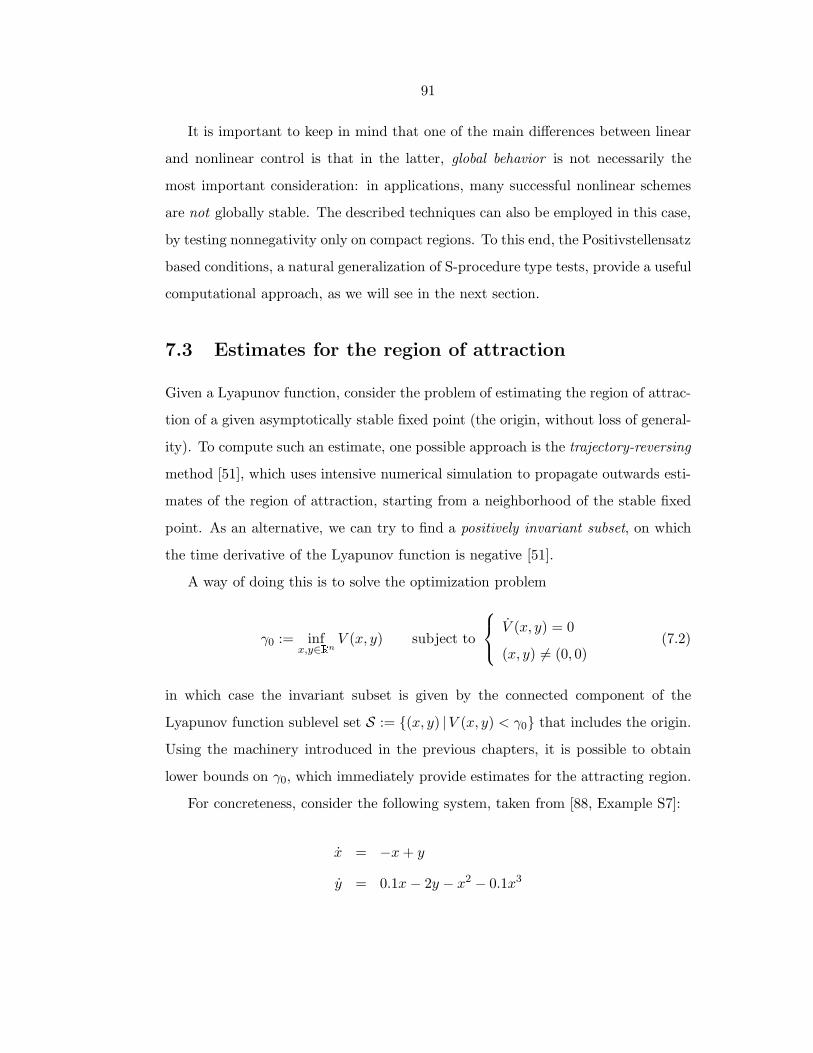
91
It is important to keep in mind that one of the main differences between linear
and nonlinear control is that in the latter, global behavior is not necessarily the
most important consideration: in applications, many successful nonlinear schemes
are not globally stable. The described techniques can also be employed in this case,
by testing nonnegativity only on compact regions. To this end, the Positivstellensatz
based conditions, a natural generalization of S-procedure type tests, provide a useful
computational approach, as we will see in the next section.
7.3 Estimates for the region of attraction
Given a Lyapunov function, consider the problem of estimating the region of attrac-
tion of a given asymptotically stable fixed point (the origin, without loss of general-
ity). To compute such an estimate, one possible approach is the trajectory-reversing
method [51], which uses intensive numerical simulation to propagate outwards esti-
mates of the region of attraction, starting from a neighborhood of the stable fixed
point. As an alternative, we can try to find a positively invariant subset, on which
the time derivative of the Lyapunov function is negative [51].
A way of doing this is to solve the optimization problem
γ0 := infx,y∈Rn
V (x, y) subject to
V (x, y) = 0
(x, y) 6= (0, 0)(7.2)
in which case the invariant subset is given by the connected component of the
Lyapunov function sublevel set S := (x, y) |V (x, y) < γ0 that includes the origin.
Using the machinery introduced in the previous chapters, it is possible to obtain
lower bounds on γ0, which immediately provide estimates for the attracting region.
For concreteness, consider the following system, taken from [88, Example S7]:
x = −x+ y
y = 0.1x − 2y − x2 − 0.1x3
92
−4 −3 −2 −1 0 1 2 3 4−3
−2
−1
0
1
2
3
x
y
Figure 7.2: Phase plot and region of attraction.
and the Lyapunov function V (x, y) := x2 + y2. The system has three fixed points,
at (0, 0), (−5 ±√
6,−5±√
6).
In [88], a lower bound estimate for γ1/20 equal to 1.911 is presented. In order to
use the methods described previously, we can consider the condition:
(V (x, y)− γ)(x2 + y2) + (p1 + p2x+ p3y + p4xy)V (x, y) is a sum of squares.
If this holds for feasible γ and pi, then obviously the bound V (x, y) ≥ γ holds for
every (x, y) satisfying the constraints in (7.2). Solving the LMIs, the optimal value
of γ1/2 is 2.66673. This actually corresponds to the optimal value, since a feasible
solution achieving this bound is given by
x ≈ −2.26099, y ≈ −1.413999.
In Figure 7.2 the vector field and the optimal level set of the Lyapunov function are
presented. The fixed points shown are the origin and (−2.55,−2.55). Notice that
the result is tight: one of the trajectories is in fact tangent to the curve V (x, y) = γ.
93
7.4 Robust bifurcation analysis
Dynamical systems possess some uniquely nonlinear phenomena, such as local bifur-
cations [92]. A vector field f(x, µ) is said to undergo a fixed point bifurcation when
the flow around a fixed point x0 changes qualitatively, when a parameter µ crosses
some critical value µ0.
Local bifurcations are very important in natural and engineered systems. For
example, in power systems it has been argued that the significant practical problem
of voltage collapse in fact has its origin in a saddle-node bifurcation, where the
operating equilibrium point suddenly disappears as a consequence of a change in the
parameters (for example, reactive load). From a practical viewpoint, is it absolutely
critical to recognize such situations, and choose nominal values for the parameters
that are far away from the hypersurface where bifurcations occur.
Despite its practical importance, there does not seem to be many systematic
approaches to the problem of computing bifurcation margins. In reference [30],
Dobson proposed two methods for computing locally closest bifurcations to a given
set of nominal parameters. These methods (iterative and direct) aim to numerically
solve the equations characterizing the closest point in the bifurcation surface. How-
ever, the problem with this approach is exactly the same as in standard robustness
analysis: what we really need in practice is some way of guaranteeing a minimum
distance (or safety margin) to a singularity, not just feasible solutions. In other
words, if we find a bifurcation “nearby,” then we need to be absolutely sure that
there are no other points that are even closer. The results in [30, 2] do not fully
address this issue: a Monte Carlo approach is employed, where the optimization is
restarted from multiple initial conditions.
The techniques developed in previous chapters can be applied to rigorously prove
bounds on the distance to the bifurcation surface. The conditions for a vector field
f(x, µ) to have a saddle-node bifurcation at (x0, µ0) are [38]:
f = 0
w∗Dxf = 0
w∗Dµf 6= 0
w∗D2xf(v, v) 6= 0
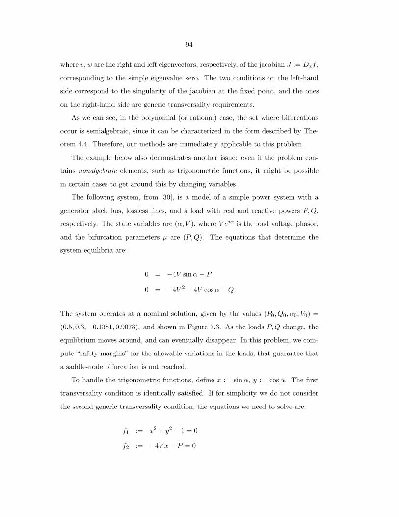
94
where v,w are the right and left eigenvectors, respectively, of the jacobian J := Dxf ,
corresponding to the simple eigenvalue zero. The two conditions on the left-hand
side correspond to the singularity of the jacobian at the fixed point, and the ones
on the right-hand side are generic transversality requirements.
As we can see, in the polynomial (or rational) case, the set where bifurcations
occur is semialgebraic, since it can be characterized in the form described by The-
orem 4.4. Therefore, our methods are immediately applicable to this problem.
The example below also demonstrates another issue: even if the problem con-
tains nonalgebraic elements, such as trigonometric functions, it might be possible
in certain cases to get around this by changing variables.
The following system, from [30], is a model of a simple power system with a
generator slack bus, lossless lines, and a load with real and reactive powers P,Q,
respectively. The state variables are (α, V ), where V ejα is the load voltage phasor,
and the bifurcation parameters µ are (P,Q). The equations that determine the
system equilibria are:
0 = −4V sinα− P
0 = −4V 2 + 4V cosα−Q
The system operates at a nominal solution, given by the values (P0, Q0, α0, V0) =
(0.5, 0.3,−0.1381, 0.9078), and shown in Figure 7.3. As the loads P,Q change, the
equilibrium moves around, and can eventually disappear. In this problem, we com-
pute “safety margins” for the allowable variations in the loads, that guarantee that
a saddle-node bifurcation is not reached.
To handle the trigonometric functions, define x := sinα, y := cosα. The first
transversality condition is identically satisfied. If for simplicity we do not consider
the second generic transversality condition, the equations we need to solve are:
f1 := x2 + y2 − 1 = 0
f2 := −4V x− P = 0
95
0
0.5
1Q
0
1
2
P
0
0.25
0.5
0.75
1
V
0
0.5Q
0
1
2
P
Figure 7.3: Equilibrium points surface and nominal operating point.
f3 := −4V 2 + 4V y −Q = 0
f4 := det J = −16V (x2 + y2 − 2V y) = 0
Since we are not interested in the case where the voltage is zero, we factor out the
first term −16V in the last equation, obtaining:
f ′4 := (x2 + y2 − 2V y) = 0
We would like, therefore, to minimize the function
J(P,Q) := (P − 0.5)2 + (Q− 0.3)2
subject to the equalities above.
Instead of dealing with the problem as a whole, since we have equality constraints
in this case it is easier to eliminate the variables that do not appear in the objective.
In other words, we will only care about the constraints we can generate that are
in the elimination ideal, i.e., 〈f1, f2, f3, f′4〉 ∩ R[P,Q]. The only reason we do this
is because of computational efficiency, but is not strictly necessary to do so from a

96
−0.5 0 0.5 1 1.5−1
−0.5
0
0.5
1
1.5
2
Q
P
P2+4Q−4=0
Figure 7.4: Curve where saddle-node bifurcations occur, and computed distance
from the nominal equilibrium.
theoretical viewpoint.
An automatic way of generating this ideal is using Grobner bases, when we use
a lexicographic degree monomial ordering [26, 64]. The elimination ideal has only
one polynomial, P 2 + 4Q − 4. This corresponds to the curve where saddle-node
bifurcations occur; see Figure 7.4. Therefore, to compute a lower bound on the
distance from the nominal equilibrium to the closest saddle-node bifurcation, we
can find the maximum γ2 that verifies the condition:
(P − 0.5)2 + (Q− 0.3)2 − γ2 + λ(P,Q)(P 2 + 4Q− 4) is a sum of squares.
In this case, it is sufficient to pick λ(P,Q) constant, and we obtain an optimal value
of γ2 ≈ 0.3735, with λ ≈ −0.2883.
To verify that the restriction to the elimination ideal is not crucial, we can easily
verify that multiplying the expressions
8V 2 + 4− 2Q, −P + 4V x, −4V y − 2 − 4 + 8V 2 + 2Q
97
by f1, f2, f3 and f ′4 respectively, and adding, we obtain the valid constraint P 2 +
4Q− 4 = 0. Therefore, the only difference in that case would be the need of using
nonconstant multipliers.
Though not guaranteed a priori by the method, in this case again we obtain a
bound that is exact. As seen in the figure, there exists a solution of the equations
that achieves the computed value of γ2, corresponding to P ≈ 0.7025, Q ≈ 0.8766.
7.5 Zero dynamics stability
When studying the global feedback linearization procedure for nonlinear systems
[46], a problem that appears is that of the zero dynamics stability. This question,
that extends the linear concepts of minimum phase, deals with the stability of the
system, when the outputs is constrained to be identically zero. At least in certain
cases, we can apply the techniques to this kind of problems. A simple example
follows.
Consider the following system, from [46, Example 4.3.4].
x1 = x3 − x32
x2 = −x2 − u
x3 = x21 − x3 + u
y = x1
(7.3)
To prove stability of the zero dynamics, it is sufficient to find a positive definite
Lyapunov function V (x), that has a negative derivative along the trajectories of
(7.3), with the constraint y ≡ 0.
Such a V can be obtained by solving the LMIs corresponding to
V (x) + λ1(x)y, −V (x) + λ2(x)y are sums of squares
A simple solution is given by V (x1, x2, x3) := 12(x2 + x3)2, since in this case the

98
second expression above reduces to:
−V (x) + x1(x2 + x3)y = (x2 + x3)2 ≥ 0.
Since the Lyapunov function and its derivative are not strictly positive, we need to
be a bit careful. However, after invoking LaSalle’s invariance principle, the stability
of the zero dynamics can be established.
7.6 Synthesis
As we have seen, the developed methods can be applied to many nonlinear analysis
questions. A natural question, therefore, is about the possibility of extending these
results to synthesis problems, where we try to find stabilizing controllers that satisfy
given performance criteria.
In the linear case, the usual LMI solution to stabilization problems goes along
the following lines [17]: to find a stabilizing controller K, we need a Lyapunov
function V (x) := xTPx, P > 0 such that A+BK is stable, i.e.,
P (A+BK) + (A+BK)TP < 0. (7.4)
This condition is not affine in both P and K. By multiplying the expression above
by Q := P−1, and defining a new variable L := KQ, we obtain:
(A+BK)Q+Q(A+BK)T = AQ+BL+ (AQ+BL)T < 0, (7.5)
which is affine in both Q and L. Since Q > 0, we can always find the controller K
as K = LQ−1.
However, extending this procedure to the nonlinear case does not seem feasible,
at least in a reasonably straightforward way. Consider an affine nonlinear system
x = f(x) + g(x)u. While the condition
∂V
∂x(f(x) + g(x)k(x)) < 0 (7.6)
99
is clearly the nonlinear equivalent of (7.4) above, there does not seem to be an
efficient way of searching simultaneously over the Lyapunov function V and the
controller k(x).
We certainly expect synthesis procedures to be no easier than the correspond-
ing analysis questions. However, the presence of additional properties, such as a
triangular structure of the vector field in simple cases of backstepping [56], usually
helps in the complexity reduction. The extent to which the presented results can
be applied in synthesis procedures still remains to be fully determined.
7.7 Conclusions
The sum of squares decomposition is a very useful sufficient condition for positivity
of a multivariable polynomial. It can be obtained at a reasonable computational
cost, using LMI methods. We can combine this procedure with Positivstellensatz
based tests, in order to extend the class of problems to which the methods are
applicable. The obtained results and procedures constitute a sound and natural
extension of standard tools in linear systems analysis. One of the big advantages
of the proposed procedure is that it is a completely algorithmic procedure. All the
computations can be carried through in a deterministic fashion, in polynomial time.
The basic idea of the procedure seems to be relevant in numerous questions
in the systems and control area. In this chapter we presented some immediate
applications, mainly dealing with the analysis of nonlinear (polynomial or rational)
systems.
In conclusion, we have shown that the combination of semialgebraic geometry
tools and semidefinite programming optimization is a very powerful general purpose
tool for dealing with the analysis of nonlinear dynamical systems.

100
101
Chapter 8
Conclusions
To conclude, we briefly summarize our main contributions, and outline some direc-
tions of future research.
8.1 Summary
In Chapter 2, an exact characterization of the optimal solution for a class of cone
preserving linear matrix inequalities was presented. The results were applied to a
variant of the rank minimization problem, and to the computation of the LMI upper
bound for the spherical µ problem.
The special structure of the LMIs arising from the Kalman-Yakubovich-Popov
lemma was exploited in Chapter 3 in the formulation of numerically efficient al-
gorithms. We introduced an outer approximation based procedure based on the
frequency domain description and a semi-infinite programming viewpoint.
From Chapter 4 on, we developed a computational framework for semialgebraic
problems, and presented applications to many different problems in systems and
control. The proposed methods are extremely general, and are based, on the one
hand, on results from real algebraic geometry, and on the other, on semidefinite
programming.
The key idea was the use a sum of squares decomposition as a sufficient condi-
tion for nonnegativity of a multivariable polynomial. This condition can be tested
in polynomial time, using LMI methods. Pairing this computational tool with the
102
Positivstellensatz in real algebraic geometry, we obtained very powerful generaliza-
tions of the successful methods developed in linear robustness analysis during the
last decade.
The problem of matrix copositivity was analyzed, and it was shown how im-
proved conditions can be obtained through the presented methodology. The en-
hanced tests were shown to be exact for a certain family of copositive quadratic
forms.
In the important specific case of indefinite quadratic programming, a new poly-
nomial time scheme for computing bounds on the optimal solution of hard nonconvex
problems was introduced. The resulting estimates are always at least as strong as
the ones obtained by the traditional semidefinite relaxation procedures.
8.2 Future research
As future research directions, it would be interesting to analyze the possibility of
extending the results in Chapter 2 to more general inequalities, and unifying several
results concerning closed forms solutions of LMIs.
Since many LMIs arising in systems and control theory do not possess the cone-
invariance property, it is interesting to examine to what extent fast algorithms can be
constructed, in the case where only part of the LMI is cone-invariant. An example
of this is the computation of µ upper bounds with mixed “norm bounded” and
“Frobenius” uncertainty block.
As we have shown, it is perfectly possible to immediately apply the tools de-
veloped in Chapter 4 to relatively small problems. However, an important issue is
certainly the computational feasibility of applying these relaxations to large scale
instances. Though in principle all the relaxations are polynomial time algorithms,
we should realize this in only a coarse characterization: in practice, other considera-
tions such as memory usage, or the actual execution time are perhaps more relevant.
In this respect, an important factor is the choice of data representation: dense cod-
ing of polynomials is clearly unsuitable for large scale problems, and alternatives
103
such as sparse representations or straight-line programs are needed.
For this reasons, more research is needed in the implementation aspects, espe-
cially on the issue of exploiting additional problem structure. Some recent inter-
esting approaches, such as the work in reference [21] on the standard MAX CUT
relaxation, show that there is lot of room for improvement, especially when working
in specific problem classes.
A natural question in the sum of squares decomposition, for instance, is if we
really need to introduce additional variables to cast the problem as an LMI, or is
it possible to solve the problem directly in the original space. After all, the set of
sum of squares polynomials is a “nice” closed convex cone. In this direction, in [66]
it has been shown that the natural self-concordant barrier for the cone of positive
definite univariate polynomials is essentially optimal.
In the general Positivstellensatz approach, another important practical issue lies
in the “customization” of the structure of the polynomial multipliers to that of the
original problem. For example, in the enhanced relaxations of Chapter 6, the homo-
geneous formulation presented in Theorem 6.1 seems natural. Also, as we have seen
in Chapter 5, in the copositivity problem some of the multipliers can be chosen with-
out loss of generality to be identically zero. Therefore, for computational reasons it
would be interesting to characterize a convenient family of possible multipliers, to
a higher level of detail than just degree bounds. In this direction, the Newton poly-
tope ideas used in sparse versions of the Nullstellensatz (see for example [87, 84])
might prove to be useful.

104

105
Appendix A
Algebra review
For the convenience of the reader, we present in this appendix some standard back-
ground material on abstract algebra. Most of the definitions are from [57, 26, 12].
Definition A.1 A group consists of a set G and a binary operation “·” defined on
G, for which the following conditions are satisfied:
1. Associative: (a · b) · c = a · (b · c), for all a, b, c ∈ G.
2. Identity: There exist 1 ∈ G such that a · 1 = 1 · a = a, for all a ∈ G.
3. Inverse: Given a ∈ G, there exists b ∈ G such that a · b = b · a = 1.
For example, the integers Z form a group under addition, but not under multiplica-
tion. Another example is the set GL(n,R) of real nonsingular n×n matrices, under
matrix multiplication.
If we drop the condition on the existence of an inverse, we obtain a monoid.
Note that a monoid always has at least one element, the identity. As an example,
given a set S, then the set of all strings of elements of S is a monoid, where the
monoid operation is string concatenation and the identity is the empty string λ.
Another example is given by N0, with the operation being addition (in this case,
the identity is the zero).
Definition A.2 A field consists of a set k and two binary operations “·” and “+”,
defined on k, for which the following conditions are satisfied:
106
1. Associative: (a+ b) + c = a+ (b+ c) and (a · b) · c = a · (b · c), for all a, b, c ∈ k.
2. Commutative: a+ b = b+ a and a · b = b · a, for all a, b ∈ k.
3. Distributive: a · (b+ c) = a · b+ a · c, for all a, b, c ∈ k.
4. Identities: There exist 0, 1 ∈ k such that a+ 0 = a · 1 = a, for all a ∈ k.
5. Additive inverse: Given a ∈ k, there exists b ∈ k such that a+ b = 0.
6. Multiplicative inverse: Given a ∈ k, a 6= 0, there exists c ∈ k such that a·c = 1.
Some commonly used fields are the rationals Q, the reals R and the complex
numbers C. There are also Galois or finite fields (the set k has a finite number of
elements), such as Zp, the set of integers modulo p, where p is a prime. Another im-
portant field if given by k(x1, . . . , xn), the set of rational functions with coefficients
in the field k, with the natural operations.
Dropping the existence of multiplicative inverses, we obtain commutative rings.
Definition A.3 A commutative ring (with identity) consists of a set k and two
binary operations “·” and “+”, defined on k, for which the following conditions are
satisfied:
1. Associative: (a+ b) + c = a+ (b+ c) and (a · b) · c = a · (b · c), for all a, b, c ∈ k.
2. Commutative: a+ b = b+ a and a · b = b · a, for all a, b ∈ k.
3. Distributive: a · (b+ c) = a · b+ a · c, for all a, b, c ∈ k.
4. Identities: There exist 0, 1 ∈ k such that a+ 0 = a · 1 = a, for all a ∈ k.
5. Additive inverse: Given a ∈ k, there exists b ∈ k such that a+ b = 0.
Any field is obviously a commutative ring. Additional examples are the integers
Z, and the polynomial ring k[x1, . . . , xn], i.e., the set of polynomials in n variables,
with coefficients in k (see Definition 4.1 in page 38).
A commutative ring is called an integral domain if it has no zero divisors, i.e.
a 6= 0, b 6= 0⇒ a ·b 6= 0. Any field is also an integral domain. Two examples of rings

107
that are not integral domains are the set of matrices Rn×n, and the set of integers
modulo n, when n is a composite number (with the usual operations). If k is an
integral domain, then so is k[x1, . . . , xn].
Definition A.4 A field k is algebraically closed if every nonconstant polynomial
in k[x1, . . . , xn] has a root in k.
The Fundamental Theorem of Algebra shows that C is an algebraically closed field.
This is not the case of R, since for example the polynomial x2 +1 does not have any
real root. To deal with the case when the base field is not algebraically closed, the
Artin-Schreier theory of formally real fields was introduced, see equation (4.12) in
Chapter 4. A related important notion is that of an ordered field:
Definition A.5 A field k is said to be ordered if a relation > is defined on k, that
satisfies
1. If a, b ∈ k, then either a > b or a = b or b > a.
2. If a > b, c ∈ k, c > 0 then ac > bc.
3. If a > b, c ∈ k, then a+ c > b+ c.
A field can be ordered if and only if it is formally real.
We consider next ideals, which are subrings with an “absorbent” property:
Definition A.6 Let R be a commutative ring. A subset I ⊂ R is an ideal if it
satisfies:
1. 0 ∈ I.
2. If a, b ∈ I, then a+ b ∈ I.
3. If a ∈ I and b ∈ R, then a · b ∈ I.
A simple example of an ideal is the set of even integers, considered as a subset of
the integer ring Z.
To introduce another important example of ideals, we need to define the concept
of an algebraic variety as the zero set of a set of polynomial equations:
108
Definition A.7 Let k be a field, and let f1, . . . , fs be polynomials in k[x1, . . . , xn].
Let the set V be
V(f1, . . . , fs) = (a1, . . . , an) ∈ kn : fi(a1, . . . , an) = 0 ∀1 ≤ i ≤ s.
We call V(f1, . . . , fs) the affine variety defined by f1, . . . , fs.
Then, the set of polynomials that vanish in a given variety, i.e.,
I(V ) = f ∈ k[x1, . . . , xn] : f(a1, . . . , an) = 0 ∀(a1, . . . , an) ∈ V ,
is an ideal, called the ideal of V .
By Hilbert’s Basis Theorem [26], k[x1, . . . , xn] is a Noetherian ring, i.e., every
ideal I ⊂ k[x1, . . . , xn] is finitely generated. In other words, there always exists
a finite set f1, . . . , fs ∈ k[x1, . . . , xn] such that for every f ∈ I, we can find gi ∈
k[x1, . . . , xn] that verify f =∑s
i=1 gifi.
We also define the radical of an ideal:
Definition A.8 Let I ⊂ k[x1, . . . , xn] be an ideal. The radical of I, denoted√I, is
the set
f | fk ∈ I for some integer k ≥ 1.
It is clear that I ⊂√I, and it can be shown that
√I is also a polynomial ideal.

109
Bibliography
[1] N. I. Akhiezer. The classical moment problem. Hafner Publishing Company,
New York, 1965.
[2] F. Alvarado, I. Dobson, and Y. Hu. Computation of closest bifurcations in
power systems. IEEE Transactions on Power Systems, 9(2):918–928, 1994.
[3] B. D. O. Anderson, N. K. Bose, and E. I. Jury. Output feedback stabilization
and related problems—solution via decision methods. IEEE Transactions on
Automatic Control, 20:53–66, 1975.
[4] M. F. Anjos and H. Wolkowicz. An strengthened SDP relaxation via
a second lifting for the MAXCUT problem. Preprint, available at
http://orion.math.uwaterloo.ca/˜hwolkowi/henry/reports/ABSTRACTS.html,
1999.
[5] M. F. Anjos and H. Wolkowicz. A tight semidefinite re-
laxation of the cut polytope. Preprint, available at
http://orion.math.uwaterloo.ca/˜hwolkowi/henry/reports/ABSTRACTS.html,
2000.
[6] V. J. D. Baston. Extreme copositive quadratic forms. Acta Arithmetica,
XV:319–327, 1969.
[7] C. A. Berenstein and D. C. Struppa. Recent improvements in the complexity of
the effective Nullstellensatz. Linear Algebra and its Applications, 157(2):203–
215, 1991.
110
[8] C. Berg. The multidimensional moment problem and semigroups. In H. J. Lan-
dau, editor, Moments in Mathematics, volume 37 of Proceedings of Symposia
in Applied Mathematics, pages 110–124. American Mathematical Society, 1987.
[9] A. Berman and R. J. Plemmons. Nonnegative Matrices in the Mathematical
Sciences. Academic Press, New York, 1979.
[10] G. Birkhoff. Linear transformations with invariant cones. Amer. Math. Monthly,
72:274–276, 1967.
[11] V. Blondel and M. Gevers. Simultaneous stabilizability of 3 linear systems is ra-
tionally undecidable. Mathematics of Control, Signals, and Systems, 6(2):135–
145, 1993.
[12] J. Bochnak, M. Coste, and M.-F. Roy. Real Algebraic Geometry. Springer, 1998.
[13] N. K. Bose. Applied multidimensional systems theory. Van Nostrand Reinhold,
1982.
[14] N. K. Bose and C. C. Li. A quadratic form representation of polynomials of sev-
eral variables and its applications. IEEE Transactions on Automatic Control,
14:447–448, 1968.
[15] S. Boyd and V. Balakrishnan. A regularity result for the singular values of a
transfer matrix and a quadratically convergent algorithm for computing its L∞norm. Systems & Control Letters, 15(1):1–7, 1990.
[16] S. Boyd, V. Balakrishnan, and P. Kabamba. A bisection method for comput-
ing the H∞ norm of a transfer matrix and related problems. Mathematics of
Control, Signals, and Systems, 2:207–219, 1989.
[17] S. Boyd, L. El Ghaoui, E. Feron, and V. Balakrishnan. Linear Matrix Inequal-
ities in System and Control Theory, volume 15 of Studies in Applied Mathe-
matics. SIAM, Philadelphia, PA, 1994.
111
[18] S. Boyd and S.-P. Wu. SDPSOL: A Parser/Solver for Semidefinite Programs
with Matrix Structure. User’s Guide, Version Beta. Stanford University, Mar.
1996.
[19] W. D. Brownawell. Bounds for the degrees in the Nullstellensatz. Annals of
Mathematics, 126:577–591, 1987.
[20] N. A. Bruinsma and M. Steinbuch. A fast algorithm to compute the H∞-norm
of a transfer function. Systems & Control Letters, 14:287–293, 1990.
[21] S. Burer and R. Monteiro. An efficient algorithm for solv-
ing the MAXCUT SDP relaxation. Preprint, available at
http://www.isye.gatech.edu/˜monteiro/tech reports/maxcut.dvi.gz,
1998.
[22] S. R. Buss and T. Pitassi. Good degree bounds on Nullstellensatz refutations
of the induction principle. Journal of computer and system sciences, 57(2):162–
171, 1998.
[23] M. D. Choi and T. Y. Lam. An old question of Hilbert. Queen’s papers in pure
and applied mathematics, 46:385–405, 1977.
[24] M. D. Choi, T. Y. Lam, and B. Reznick. Sums of squares of real polynomials.
Proceedings of Symposia in Pure Mathematics, 58(2):103–126, 1995.
[25] R. W. Cottle, J. S. Pang, and R. E. Stone. The linear complementarity problem.
Academic Press, 1992.
[26] D. A. Cox, J. B. Little, and D. O’Shea. Ideals, varieties, and algorithms:
an introduction to computational algebraic geometry and commutative algebra.
Springer, 1997.
[27] J. de Loera and F. Santos. Correction of errors to: An effective
version of Polya’s theorem on positive definite forms. Available at
http://www.matesco.unican.es/˜santos/Articulos/JPAAcorr.ps.gz, to
appear in J. Pure Appl. Algebra.

112
[28] J. de Loera and F. Santos. An effective version of Polya’s theorem on positive
definite forms. J. Pure Appl. Algebra, 108:231–240, 1996.
[29] P. H. Diananda. On non-negative forms in real variables some or all of which
are non-negative. Proceedings of the Cambridge Philosophical Society, 58:17–25,
1962.
[30] I. Dobson. Computing a closest bifurcation instability in multidimensional pa-
rameter space. Nonlinear Science, 3:307–327, 1993.
[31] P. Dorato, W. Yang, and C. Abdallah. Robust multi-objective feedback design
by quantifier elimination. J. Symbolic Computation, 24:153–159, 1997.
[32] M. Fu. The real structured singular value is hardly approximable. IEEE Trans-
actions on Automatic Control, 42(9):1286–1288, 1997.
[33] M. Fu. Comments on “A procedure for the positive definiteness of forms of even
order”. IEEE Transactions on Automatic Control, 43(10):1430, 1998.
[34] P. Gahinet and P. Apkarian. A linear matrix inequality approach toH∞ control.
International Journal of Robust and Nonlinear Control, 4(4):421–448, 1994.
[35] P. Gahinet, A. Nemirovski, A. J. Laub, and M. Chilali. LMI Control Toolbox.
The MathWorks Inc., Natick, Mass., May 1995.
[36] M. R. Garey and D. S. Johnson. Computers and Intractability: A guide to the
theory of NP-completeness. W. H. Freeman and Company, 1979.
[37] M. X. Goemans and D. P. Williamson. Improved approximation algorithms
for maximum cut and satisfiability problems using semidefinite programming.
Journal of the ACM, 42(6):1115–1145, 1995.
[38] J. Guckenheimer and P. Holmes. Nonlinear Oscillations, Dynamical Systems,
and Bifurcations of Vector Fields. Springer-Verlag, 1983.
[39] M. Hall and M. Newman. Copositive and completely copositive quadratic forms.
Proc. Camb. Phil. Soc., 59:329–339, 1963.

113
[40] G. H. Hardy, J. E. Littlewood, and G. Polya. Inequalities. Cambridge University
Press, 1967.
[41] M. A. Hasan and A. A. Hasan. A procedure for the positive definiteness of
forms of even order. IEEE Transactions on Automatic Control, 41(4):615–617,
1996.
[42] D. S. Hochbaum, editor. Approximation algorithms for NP-hard problems. PWS
Publishing Company, 1997.
[43] D. A. Holton and J. Sheehan. The Petersen graph, volume 7 of Australian
Mathematical Society Lecture Series. Cambridge University Press, 1993.
[44] R. A. Horn and C. R. Johnson. Matrix Analysis. Cambridge University Press,
Cambridge, 1995.
[45] Y. Huang. Nonlinear Optimal Control: An Enhanced Quasi-LPV Approach.
PhD thesis, California Institute of Technology, 1998.
[46] A. Isidori. Nonlinear Control Systems. Springer-Verlag, Berlin, third edition,
1997.
[47] M. Jirstrand. Nonlinear control system design by quantifier elimination. J. Sym-
bolic Computation, 24:137–152, 1997.
[48] M. Johansson. Piecewise Linear Control Systems. PhD thesis, Lund Institute
of Technology, 1999.
[49] M. Johansson and A. Rantzer. Computation of piecewise quadratic lya-
punov functions for hybrid systems. IEEE Transactions on Automatic Control,
43(4):555–559, 1998.
[50] U. Jonsson and A. Rantzer. Duality bounds in robustness analysis. Automatica,
33(10):1835–1844, 1997.
[51] H. Khalil. Nonlinear Systems. Macmillan Publishing Company, 1992.
114
[52] S. Khatri and P. A. Parrilo. Spherical µ. In Proceedings of the American Control
Conference, 1998.
[53] J. Kollar. Sharp effective Nullstellensatz. J. Amer. Math. Soc., 1:963–975, 1988.
[54] A. N. Kolmogorov and S. V. Fomin. Introductory Real Analysis. Dover, 1970.
[55] M. G. Krein and M. A. Rutman. Linear operators leaving invariant a cone in
a Banach space. Usp. Mat. Nauk (N.S), 3:3–95, 1948. (English transl.: Amer.
Math. Soc. Transl. Ser. I, vol. 10, (1962), 199–325).
[56] M. Krstic, I. Kanellakopoulos, and P. V. Kokotovic. Nonlinear and Adaptive
Control Design. John Wiley & Sons, 1995.
[57] S. Lang. Algebra. Addison-Wesley, 1971.
[58] L. Lovasz. Stable sets and polynomials. Discrete mathematics, 124:137–153,
1994.
[59] L. Lovasz and A. Schrijver. Cones of matrices and set-functions and 0-1 opti-
mization. SIAM Journal on Optimization, 1(2):166–190, 1991.
[60] A. Megretski, C.-Y. Kao, U. Jonsson, and A. Rantzer. A Guide To IQCβ:
Software for Robustness Analysis, June 1998.
[61] A. Megretski and A. Rantzer. System analysis via Integral Quadratic Con-
straints. IEEE Transactions on Automatic Control, 42(6):819–830, 1997.
[62] M. Mesbahi. On the rank minimization problem and its control applications.
Systems & Control Letters, 33:31–36, 1998.
[63] M. Mesbahi and G. P. Papavassilopoulos. On the rank minimization problem
over a positive semidefinite linear matrix inequality. IEEE Transactions on
Automatic Control, 42(2):239–243, 1997.
[64] B. Mishra. Algorithmic Algebra. Springer-Verlag, 1993.
115
[65] K. G. Murty and S. N. Kabadi. Some NP-complete problems in quadratic and
nonlinear programming. Mathematical Programming, 39:117–129, 1987.
[66] Y. Nesterov. Squared functional systems and optimization problems. In
J. Frenk, C. Roos, T. Terlaky, and S. Zhang, editors, High Performance Opti-
mization, pages 405–440. Kluwer Academic Publishers, 2000.
[67] Y. E. Nesterov and A. Nemirovski. Interior point polynomial methods in convex
programming, volume 13 of Studies in Applied Mathematics. SIAM, Philadel-
phia, PA, 1994.
[68] E. E. Osborne. On preconditioning of matrices. Journal of the Assoc. for Comp.
Mach., 7:338–349, 1960.
[69] A. Packard and J. C. Doyle. The complex structured singular value. Automatica,
29(1):71–109, 1993.
[70] C. H. Papadimitriou and K. Steiglitz. Combinatorial Optimization: Algorithms
and Complexity. Dover, 1998.
[71] M. Petkovsek, H. S. Wilf, and D. Zeilberger. A=B. A.K. Peters Ltd., 1996.
[72] E. Polak. Optimization: Algorithms and Consistent Approximations, volume
124 of Applied Mathematics Sciences. Springer, 1997.
[73] V. Powers and B. Reznick. A new bound for Polya’s theorem with ap-
plications to polynomials positive on polyhedra. Preprint, available at
http://www.mathcs.emory.edu/˜vicki/preprint/polya.ps, 2000.
[74] V. Powers and T. Wormann. An algorithm for sums of squares of real polyno-
mials. Journal of pure and applied algebra, 127:99–104, 1998.
[75] A. J. Quist, E. De Klerk, C. Roos, and T. Terlaky. Copositive relaxation for
general quadratic programming. Optimization methods and software, 9:185–
208, 1998.
116
[76] A. R. Rajwade. Squares, volume 171 of London Mathematical Society Lecture
Note Series. Cambridge University Press, 1993.
[77] A. Rantzer. On the Kalman-Yakubovich-Popov lemma. Systems & Control Let-
ters, 28:7–10, 1996.
[78] B. Reznick. Extremal PSD forms with few terms. Duke Mathematical Journal,
45(2):363–374, 1978.
[79] B. Reznick. Uniform denominators in Hilbert’s seventeenth problem. Math Z.,
220:75–97, 1995.
[80] B. Reznick. Some concrete aspects of Hilbert’s 17th problem. Preprint, available
at http://www.math.uiuc.edu/Reports/reznick/98-002.html, 1999.
[81] K. Schmudgen. The k-moment problem for compact semialgebraic sets. Math.
Ann., 289:203–206, 1991.
[82] H. D. Sherali and W. P. Adams. A hierarchy of relaxations between the con-
tinuous and convex hull representations for zero-one programming problems.
SIAM J. Disc. Math., 3(3):411–430, 1990.
[83] N. Z. Shor. Class of global minimum bounds of polynomial functions. Cyber-
netics, 23(6):731–734, 1987. (Russian orig.: Kibernetika, No. 6, (1987), 9–11).
[84] M. Sombra. A sparse effective Nullstellensatz. Advances in Applied Mathemat-
ics, 22:271–295, 1999.
[85] G. Stengle. A Nullstellensatz and a Positivstellensatz in semialgebraic geometry.
Math. Ann., 207:87–97, 1974.
[86] J. Sturm. SeDuMi version 1.03., Sept. 1999. Available from
http://www.unimaas.nl/˜sturm/software/sedumi.html.
[87] B. Sturmfels. Polynomial equations and convex polytopes. American Mathe-
matical Monthly, 105(10):907–922, 1998.
117
[88] A. Tesi, F. Villoresi, and R. Genesio. On the stability domain estimation via
a quadratic Lyapunov function: convexity and optimality properties for poly-
nomial systems. IEEE Transactions on Automatic Control, 41(11):1650–1657,
1996.
[89] O. Toker. On the algorithmic unsolvability of some stability problems for hybrid
systems. IEEE Transactions on Automatic Control, 45(1):165–168, 2000.
[90] H. Valiaho. Criteria for copositive matrices. Linear Algebra and its applications,
81:19–34, 1986.
[91] L. Vandenberghe and S. Boyd. Semidefinite programming. SIAM Review,
38(1):49–95, Mar. 1996.
[92] S. Wiggins. Introduction to applied nonlinear dynamical systems and chaos.
Springer-Verlag, New York, 1990.
[93] J. C. Willems. Least squares stationary optimal control and the algebraic Ric-
cati equation. IEEE Transactions on Automatic Control, 16(6):621–634, 1971.