PHYSICAL REVIEW FLUIDS 2, 064602 (2017)

Structure function tensor scaling in the logarithmic region derived fromthe attached eddy model of wall-bounded turbulent flows

X. I. A. Yang,1 R. Baidya,2 P. Johnson,1 I. Marusic,2 and C. Meneveau1

1Department of Mechanical Engineering, Johns Hopkins University, Baltimore, Maryland 21218, USA2Department of Mechanical Engineering, University of Melbourne, Parkville, VIC, 3010, Australia

(Received 9 March 2017; published 5 June 2017)

We investigate the scaling of the velocity structure function tensor Dij (r,z) in highReynolds number wall-bounded turbulent flows, within the framework provided by theTownsend attached eddy hypothesis. Here i,j = 1,2,3 denote velocity components in thethree Cartesian directions, and r is a general spatial displacement vector. We considerspatial homogeneous conditions in wall-parallel planes and dependence on wall-normaldistance is denoted by z. At small scales (r = |r| � z) where turbulence approaches localisotropy, Dij (r,z) can be fully characterized as a function of r and the height-dependentdissipation rate ε(z), using the classical Kolmogorov scalings. At larger distances in thelogarithmic range, existing previous studies have focused mostly on the scaling of Dij forr in the streamwise direction and for the streamwise velocity component (i = j = 1) only.No complete description is available for Dij (r,z) for all i,j , and r directions. In this paperwe show that the hierarchical random additive process model for turbulent fluctuations inthe logarithmic range (a model based on the Townsend’s attached eddy hypothesis) maybe used to make new predictions on the scaling of Dij (r,z) for all velocity componentsand in all two-point displacement directions. Some of the generalized scaling relationsof Dij (r,z) in the logarithmic region are then compared to available data. Nevertheless, anumber of predictions cannot yet be tested in detail, due to a lack of simultaneous two-pointmeasurements with arbitrary cross-plane displacements, calling for further experiments tobe conducted at high Reynolds numbers.

DOI: 10.1103/PhysRevFluids.2.064602

I. INTRODUCTION

The most basic statistical characterization of turbulence structure is encoded in the two-pointcorrelation or two-point structure functions of the turbulent velocity field. At small scales, withdisplacements in the inertial range of turbulence, a universal form is available from the Kolmogorovscaling [1,2]. In wall-bounded flows, at scales comparable to the distance from the wall in thelogarithmic region, very significant deviations from local isotropy develop. We lack a suitably generaldescription of anisotropic energy containing motions, and the present work is devoted to this topic.

Wall-bounded flows, particularly flows at high Reynolds numbers, have been the subject ofsustained research efforts (see, e.g., Refs. [3–5] for reviews), and predictive reduced-order modelsare extensively available in the literature [6–14]. A fairly established conceptual model for highReynolds number wall-bounded turbulent flows is the Townsend attached eddy model [6], in whichthe logarithmic region is modeled as a collection of self-similar, wall-attached eddies, whose sizesscale with their distance from the wall (see Fig. 1). Despite its simple form, this model has beenquite useful. Invoking the attached eddy hypothesis, not only can the logarithmic scaling of themean velocity profile be derived, but Townsend [6] also derived the logarithmic scalings for 〈u2〉 ∼log(δ/z), 〈v2〉 ∼ log(δ/z), where u and v are the velocity fluctuations in the streamwise and spanwisedirections, δ is an outer length scale, and z is the wall-normal coordinate. To date, these twogeneralized logarithmic scalings have received considerable empirical support [15–19]. The attachededdy picture also permits scaling laws including 〈�u2〉 ∼ log(rx/z), 〈u(x)u(x + rx)〉 ∼ log(δ/rx),which have been confirmed recently in de Silva et al. [20] and Yang et al. [21], respectively. Here

2469-990X/2017/2(6)/064602(18) 064602-1 ©2017 American Physical Society

YANG, BAIDYA, JOHNSON, MARUSIC, AND MENEVEAU

FIG. 1. Conceptual schematic diagram of the attached eddy model of high Reynolds number turbulentboundary layer flows. The number of visible eddies on a vertical cut doubles as the sizes of the eddies halve.An attached eddy affects the shaded region. A realization of the velocity fluctuation at a generic point in theflow field is given by a superposition of the velocity fields associated with the attached eddies within whichthe generic point locates. Inclination of the attached eddies leads to a lag in the velocity signal between twowall-normal locations, as indicated in the sketch.

�u = u(x + rx) − u(x), rx is a streamwise displacement and x is the streamwise coordinate. Inaddition to these logarithmic scalings, the k−1

x spectrum in the logarithmic region is also a directconsequence of the presence of wall-attached eddies [22]. More recently, the attached-eddy model hasbeen extended to account for more detailed observations, including wake effects and eddy clusteringphenomena (see, e.g., Refs. [7,8]), as well as logarithmic scalings of higher order moments [20,23].

More generally, the statistics of turbulent flows are fully specified by all N -point M-ordercorrelation functions [24], or equivalently, the related structure functions. Structure functions werefound to be particularly useful for studying homogeneous isotropic turbulence, where an exactrelation holds connecting the third-order structure function to the second order as a function of thedissipation rate [1]. Furthermore, we remark that knowledge of the scalings of the structure functionscan be used to provide estimates on the coarse-grained velocity gradients, subfilter stresses, andhigher order subscale cumulants [25–27], which has implications for subgrid-scale modeling andlarge-eddy simulations, where eddies of any particular scale in wall units become more and moresubgrid (unresolved) as the Reynolds number increases. Moreover, a second-order spatial statisticaldescription can be leveraged to model the full spatio-temporal structure [28,29] of the flow.

In this work we consider the two-point, second-order structure function defined as

Dij (x,r) = 〈(ui(x + r) − ui(x))(uj (x + r) − uj (x))〉. (1)

For incompressible homogeneous isotropic turbulence, this tensor could be fully specified with ascalar function DLL(r) (the longitudinal structure function) [2,24], which in turn only dependson r and the mean rate of dissipation ε in the inertial range (with the formula being Dij =DLLδij + r/2∂DLL/∂r(δij − rirj /r2), where δij is the second-order identity tensor). The localisotropic behavior is expected to hold in wall-bounded turbulence for displacements much smallerthan the height z above the wall [20,30–32]. As the dissipation in the logarithmic region canbe evaluated assuming equilibrium between production and dissipation, the z dependence of thelongitudinal structure function is encoded in ε(z) ∼ u3

τ /z. On the other hand for displacementslarger than the height (r > z), i.e., for the energy-containing and momentum-transporting motions,turbulence becomes anisotropic and inhomogeneous so that simplifications associated with isotropyare not possible, and the specification of the second-order structure functions becomes less simple.

Structure functions in wall-bounded flows have been considered from a theoretical viewpointby Hill [33] and Cimarelli et al. [34] as part of derivations of a generalized Kolmogorov equation

064602-2

STRUCTURE FUNCTION TENSOR SCALING IN THE . . .

allowing for nonhomogeneity and anisotropy. From an experimental viewpoint, structure functionshave been studied in recent works by Davidson [32] and de Silva et al. [20]. These prior efforts havefocused primarily on the streamwise direction, i.e., the special case r = (rx,0,0) and i = j = 1.

The attached eddy model for energy containing motions in wall-bounded flows is analogous [35]to the eddy hierarchy cascade models for isotropic homogeneous turbulence [2]. It describes thestatistical structure of turbulent motions in a given range by providing a method for calculatingstatistics based on randomly distributed wall-attached, momentum-transferring eddies with a chosencharacteristic eddy shape, and a prescribed density depending on distance to the wall. As a resultit allows for scaling predictions over a certain range of scales in wall-bounded turbulence. Whilepreviously, only scalings of the streamwise velocity component with streamwise displacements wereconsidered in the attached eddy model, predictions can also be made for other velocity componentsincluded in other Reynolds stresses, as shown in Refs. [7,8]. However, for structure functions inarbitrary directions and for all three velocity components, scaling predictions have not yet beenestablished based on the attached eddy model. Given the success of the model in the context ofstreamwise statistics, it is of interest to extend scaling predictions to other directions and velocitycomponents. This is the main objective of the work presented here.

We develop predictions on the scalings of the full structure function tensor Eq. (1), for x in thelogarithmic region and for relevant ranges of the two-point displacement r such that x + r is alsoin the log region (see Ref. [36] for detailed discussion on the extent of the log region). ui , uj arethe velocity fluctuations in xi , xj directions; i,j = 1,2,3. We first consider the full specification of ageneral second-order structure function under the specific conditions that the wall-normal coordinateis denoted by a unit vector z, and the direction of the free stream velocity is given by a unit vector u.Because of the translational symmetry on wall-parallel planes, the dependency of Dij on x is reducedto z = x · z, where z is the wall-normal component of x. The two-point displacement vector r maybe in any direction. In general, the symmetric, x, z, and r-dependent tensor Dij may be expressed as

Dij (r,z) = D11(rx,ry,rz,z)ui uj + D12(·)(ui tj + uj ti) + D13(·)(ui zj + uj zi) + D22(·)ti tj+D23(·)(ti zj + tj zi) + D33(·)zi zj , (2)

where t = z × u (unit vectors u and z are orthogonal), u, z, and t form a rectangular coordinatesystem, D11, D12, D13, D22, D13, and D33 are scalar functions of z, rx = r · u, ry = r · t, rz = r · zand the friction velocity uτ (or magnitude of the free-stream velocity). As Dij is symmetric undercoordinate system reflection, terms depending on t have to vanish, i.e., D12 = D23 = 0. Note thataccording to the theory of homogeneous tensors, a symmetric tensor that depends on three vector(z, u, r) takes the form

Dij (r,z) = fδδij + fuuui uj + fzzzi zj + frr ri rj + fur12 (ui rj + uj ri) + fuz

12 (ui zj + uj zi)

+ fzr12 (zi rj + zj ri), (3)

where the f are scalar functions of a number of scalar quantities that can be formed from the vectorsr, u, z and the distance z. As a constraint in this problem, the vectors u and z are perpendicular to eachother, introducing additional conditions. Since the above general tensor requires the specification ofseven instead of four scalar functions [as in Eq. (2)], we opt to use Eq. (2).

Throughout the paper, we denote x1, x2, x3 as the streamwise, spanwise, and wall-normalcoordinates, respectively; we interchangeably use u, v, w for the velocity fluctuations in thestreamwise, spanwise, and wall-normal directions; x, y, z are interchangeably used for x1, x2, x3. Asstated above, the displacement r = (

rx,ry,rz

), and rz > 0. In this paper, velocities are normalized by

the friction velocity uτ , and normalization with viscous length scale ν/uτ (where ν is the kinematicviscosity) will be indicated by a + superscript. We consider only velocity fluctuations. As mentionedbefore, prior work has focused mostly on the dependence of D11 upon rx . As can be seen above, forthe full specification of the generalized structure function, we also require expressions for the scalarfunctions D22, D33, and D13, all as functions of (rx,ry,rz,z). As shown by Hill [33], incompressibility

064602-3

YANG, BAIDYA, JOHNSON, MARUSIC, AND MENEVEAU

imposes the following constraint on the structure function:

∂Dij (r,z)

∂rj

= 1

2

∂

∂x3〈[ui(x + r) + ui(x)][u3(x + r) − u3(x)]〉, (4)

which involves moments other than the structure functions themselves, and thus we will not exploitincompressibility as a useful constraint.

In Sec. II, we summarize the hierarchical random additive process as a model for wall-boundedturbulent velocity fluctuations in the logarithmic range and in Sec. III show how it can be used tomake predictions about the general scaling of these functions. We will invoke the simplest possiblemodeling assumptions and state the resulting specific predictions. We will then attempt to verifythe predicted trends in Sec. IV. Several of the required measurements are available only from DNSat moderate to intermediate Reynolds numbers so the discussion in Sec. IV cannot be consideredconclusive. We leave open the possibility that once measurements become available at high Reynoldsnumbers, the various simplifying assumptions made in the simplest version of the proposed modelmay need further refinement.

II. THE HIERARCHICAL RANDOM ADDITIVE PROCESS (HRAP) MODEL

The HRAP is a simplified version of the Townsend attached eddy model, in which the eddy-induced velocity fields are modeled as random addends. The wall-parallel velocity components ata wall-normal distance z include additive contributions from eddies whose heights are greater thanz. Conversely, for the wall-normal component, the contributions from large eddies whose heightsare greater than z are severely blocked by the presence of the wall, and only contributions fromeddies of a size comparable to z count. Accordingly, the HRAP formalism models the instantaneousstreamwise and spanwise velocity fluctuations at a given position and height z as a result of randomadditive processes according to

u =Nz∑i=1

ai, v =Nz∑i=1

bi. (5)

A random addend ai (or bi) represents the velocity increment in u (or v) due to an attached eddyof height ∼δ/2i , where δ is the height of the largest wall attached eddy that the boundary layer canadmit (typically on the order of the outer boundary layer thickness). The instantaneous wall-normalvelocity fluctuation is modeled as the negative of the last addend in the construction leading to u:

w = −aNz. (6)

This last step ensures a negative correlation so that the mean momentum flux is constant in the logregion:

〈uw〉 =Nz∑i=1

〈aiaNz〉 = −⟨

a2Nz

⟩ = −〈a2〉. (7)

A notional attached eddy is sketched in Fig. 2 and a top view of the modeled flow field is sketchedin Fig. 3. By relating ai with an attached eddy of height δ/2i , we have discretized the boundary layerlogarithmically in the wall-normal direction. The base 2 is arbitrary but convenient and is chosen forconsistency with Ref. [37]. We now make an additional geometric assumption about the aspect ratioof the wall-attached eddies. We assume that wall-attached eddies at a height h may be characterizedby lengths lx and ly in the streamwise and spanwise directions, respectively. Therefore, an attachededdy of height h affects two points which lie nominally within the lx × ly area of influence (cf. Fig. 2).Let us further denote the aspect ratio R = ly/ lx as a given, z-independent geometric constant (forempirical evidence for geometric self-similarity in the logarithmic region, see, e.g., recent detailedanalyses of DNS by del Álamo et al. [38]). In other words, two points such that z < h, z + rz < h,

064602-4

STRUCTURE FUNCTION TENSOR SCALING IN THE . . .

FIG. 2. Conceptual sketch of a notional attached eddy of height z. This eddy extends and affects an areaof lx × ly (in x × y plane). The inclination angle of this eddy is θ . lx = z/ tan(θ ). Define R = ly/ lx to bethe aspect ratio, it follows that ly = Rz/ tan(θ ). Because of the assumed similarity, R, θ are z-independentgeometric constants.

rx < h/ tan(θ ), ry < Rh/ tan(θ ) share all addends from eddies of height greater than h. Such acompact representation of eddy-induced velocity fluctuations allows us to make predictions on thescalings of various flow statistics in the logarithmic region, where the eddies are self-similar, andthe random addends ai are statistically identical, as are the addends bi (see Refs. [23,39] for detaileddiscussion).

We assume that large-scale eddies do not directly interact with small-scale eddies, and that ai ,aj , i �= j are statistically independent (so are bi , bj , i �= j ). ai and bi are therefore independentrandom variables, each of which are identically distributed (but ai and bi possibly have differentdistributions). Neglecting interscale interactions (or interactions among different heights) must behere considered as a first approximation. Amplitude modulation effects [40,41] observed in thevicinity of the wall have not yet been explored in detail among scales and eddies in the log region.To the degree that they occur, these can be considered as a higher-order corrections to the simplestapproximation made here of assuming independence. Furthermore, amplitude modulation is animportant process for odd-order statistics, but for second-order statistics, accounting for the effectsof modulation or not does not make a significant difference [42]. At a distance z from the wall, theinfluence of an attached eddy of size � z becomes negligible, and therefore the number of randomaddends in Eq. (5) can simply be obtained by integrating the eddy population density P (z) ∼ 1/z

FIG. 3. Top view of the modeled wall-bounded flow showing a random superposition of notional wallattached eddies. Wall eddies tend to be stretched in the flow direction. Because eddy population density isinversely proportional to the wall-normal distance, the number of observable eddies on an x-y plane quadruplesas the sizes of the eddies halve. Wall-attached eddies of different sizes are colored differently.

064602-5

YANG, BAIDYA, JOHNSON, MARUSIC, AND MENEVEAU

from z to δ, leading to

Nz ∼∫ δ

z

P (z) ∼ log(δ/z). (8)

As an example of possible applications of the HRAP model, we compute 〈u2〉, 〈v2〉. Squaring bothsides of Eq. (5) leads to

〈u2〉 = Nz〈a2〉 ∼ log(δ/z) = A1 log(δ/z) + B1,(9)

〈v2〉 = Nz〈b2〉 ∼ log(δ/z) = A1,v log(δ/z) + B1,v,

recovering the logarithmic scaling for 〈u2z〉 and 〈v2

z 〉. Here, A1, A1,v , B1, and B1,v are constants.The value of A1, the Townsend-Perry constant, has been determined empirically, yielding A1 ≈1.2–1.3 [36]. In this work, Eqs. (5), (6), and (8) are used to provide estimates for all scalar functionsin Eq. (2).

III. SCALING OF GENERAL TWO-POINT STRUCTURE FUNCTIONS

We begin by defining the “associated eddy height” corresponding to particular (specified)horizontal displacements rx and, separately, ry . Specifically, we define

zrx = |rx | tan(θ ), zry = |ry |R

tan(θ ). (10)

The height zrx is the minimum height of an eddy that can simultaneously affect two points with adisplacement rx only in the streamwise direction. In other words, two points separated by a distance rx

can be affected only by an eddy with a height greater than zrx . Similarly, for displacements only in thetransverse direction ry , zry is the height corresponding to an eddy of x-direction length ry/R. For nowwe are assuming these two heights are smaller than δ. For arbitrary displacements rx and ry , we define

zc = min{max[|rx |,|ry |/R] tan(θ ),δ}, (11)

which is the minimum height of an eddy that simultaneously affects two points at a distance rx , ry inthe x, y directions, given that the boundary layer can not admit eddies higher than δ. We assume thatthe displacements are larger than a minimum value so that the velocity fluctuations at the two pointsdiffer at least by one addend. For smaller displacements, the two-points are considered equivalentin the framework of HRAP, and the associated structure function follows the inertial-range scalings.

Applying the HRAP model to determine D11(rx,ry,rz,z), we must determine the number ofcommon addends shared by the two points. For this purpose we focus on the vertical locationof the higher point, at z + rz (rz > 0). Depending on rx and ry , we can identify three regimes(see Fig. 4):

I : zc < z + rz, II : z + rz < zc < δ, III : zc = δ. (12)

For two points in regime III, the points share no common eddy, hence

D11 =˝⎛⎝ Nz∑

i=1

a′i −

Nz+rz∑i=1

a′′i

⎞⎠

2˛= (

Nz + Nz+rz

)〈a2〉 − 2

˝(Nz∑i=1

a′i

)·⎛⎝Nz+rz∑

i=1

a′′i

⎞⎠˛

= (Nz + Nz+rz

)〈a2〉 = A1 log

(δ

z

)+ A1 log

(δ

z + rz

)+ C3. (13)

064602-6

STRUCTURE FUNCTION TENSOR SCALING IN THE . . .

FIG. 4. Examples of pairs of points in regimes I, II, and III. For two points in regime III (indicated as pointsIII1, III2), III1 shares none of its addends with III2. For two points in regime I (indicated as points I1, I2), I1

share all common addends with I2 (and then I1 includes an extra addend since it is closer to the wall). For twopoints in regime II (II1, II2), II1 share part of the addends with II2 (specifically in this example, addends fromeddies of height δ, δ/2). The schematic is in accordance with Fig. 1. As is sketched in Fig. 1, a horizontal linecorresponds to an eddy and affects the region below it. While the sketch is artificially regular for purposes ofillustration, in reality the model encompasses more random spatial arrangements of eddies as in Fig. 3.

For two points in regime I, point x share all the eddies that affect x + r (0 < rz), hence

D11 =˝⎡⎣

⎛⎝Nz+rz∑

i=1

ai +Nz∑

i=Nz+rz

a′i

⎞⎠ −

⎛⎝Nz+rz∑

i=1

ai

⎞⎠

⎤⎦

2˛

=˝⎡⎣ Nz∑

i=Nz+rz

a′i

⎤⎦

2˛= (

Nz − Nz+rz

)〈a2〉 = A1 log

(z + rz

z

)+ C1. (14)

Note that we are excluding from these considerations the transition towards the locally isotropicscaling that occurs when r = (r2

x + r2y + r2

z )1/2 < Czz, where Cz is an O(1) constant. For regime I,typically rx and ry are small and therefore we must limit rz to be (typically) larger than z. Thus thescaling implied by Eq. (14) is meant to hold for rz/z � 1. In the limit rz/z � 1, a transition towardsthe inertial range scaling is envisioned.

For two points in regime II, points (x,y,z) and (x + rx,y + ry,z + rz) share the eddies of heightgreater than zc, hence

D11 =˝⎡⎣

⎛⎝ Nzc∑

i=1

ai +Nz∑

i=Nzc

a′i

⎞⎠ −

⎛⎝ Nzc∑

i=1

ai +Nz+rz∑i=Nzc

a′′i

⎞⎠

⎤⎦

2

=˝⎡⎣ Nz∑

i=Nzc

a′i −

Nz+rz∑i=Nzc

a′′i

⎤⎦

2˛

= (Nz − Nzc

)〈a2〉 + (Nz+rz

− Nzc

)〈a2〉 − 2

˝⎛⎝ Nz∑

i=Nzc

a′i

⎞⎠ ·

⎛⎝Nz+rz∑

i=Nzc

a′′i

⎞⎠˛

= (Nz − Nzc

)〈a2〉 + (Nz+rz

− Nzc

)〈a2〉 = A1 log

(zc

z

)+ A1 log

(zc

z + rz

)+ C2, (15)

where a, a′, a′′ are i.i.d. variables. Imposing continuity of D11 with respect to zc, it is clear that theconstants C1, C2, C3 must be equal,

C1 = C2 = C3. (16)

It is worth noting that, although we have discretized the log region into discrete hierarchical scalesand both Nz, Nz+rz

are integers that take only discrete values, because in Eq. (8) the integration isa continuous function of z, the predictions here are continuous functions of z and r. Combining

064602-7

YANG, BAIDYA, JOHNSON, MARUSIC, AND MENEVEAU

FIG. 5. (a) A sketch of the various regimes used to evaluate the scaling of D11 under the HRAP simplifiedattached eddy model. The definition of zc is cut off at δ, therefore regime III is indicated only at zc = δ. z + rz isrequired to be in the boundary layer, i.e., z + rz < δ. (b) Contour levels computed according to Eq. (18) for D11

as a function of zc and z + rz for z = 0.01δ, using A1 = 1.25 and setting C11 = 2 for purposes of illustration.

Eqs. (12)–(16), we have

D11 = A1 log

(z + rz

z

)+ C11, zc < z + rz,

D11 = A1 log

(zc

z

)+ A1 log

(zc

z + rz

)+ C11, z + rz < zc < δ, (17)

D11 = A1 log

(δ

z

)+ A1 log

(δ

z + rz

)+ C11, zc = δ,

where C11 is a constant. Defining ze = max [zc,z + rz], a compact form of D11 is

D11 = A1 log

(ze

z

)+ A1 log

(ze

z + rz

)+ C11, (18)

where we recall that z and z + rz are assumed to fall in the logarithmic layer, i.e., significantlybelow δ.

The various regimes are sketched in Fig. 5(a). Essentially we seek the minimum height hc ofan eddy that can simultaneously affect the two points under consideration. Because of the treelikeorganization of the attached eddies, the effects of eddies with height h > hc is canceled (becausewe are taking the difference between the two points when evaluating structure functions). Effects ofeddies of heights h < hc remain and are reflected separately on two points, in the form

log

(hc

z

)+ log

(hc

z + rz

). (19)

It is useful to point out that hc is not necessarily equal to zc since zc is the minimum height of an eddythat could affect two points with a displacement rx , ry in the x, y directions. The two points could bedisplaced by a very small distance in the x-y plane but by a large distance in the vertical direction.In that case, hc becomes z + rz and we are in regime I. Regime II is straightforward, where zc = hc.If the two points are so separated that to affect them simultaneously one needs an eddy of heightgreater than δ, then we are in regime III. The description stops at zc = hc = δ (since the boundarylayer does not admit any eddy whose height is greater than δ). A sketch of D11 as a function of zc

and z + rz is shown in Fig. 5(b). The contour levels are computed according to Eq. (18). The hiddenparameter z is 0.01δ, which is chosen arbitrarily for illustration purposes.

A few asymptotes of Eq. (17) have been investigated previously. For example, taking rz = 0 andrx δ (and/or ry δ), we have zc = δ, ze = δ and we obtain D11 = 2A1 log(δ/z) + C11, i.e., thelogarithmic scaling of 〈u2〉 = 1

2D11(|r| δ,z) as a function of z is recovered. Taking rz = ry = 0

064602-8

STRUCTURE FUNCTION TENSOR SCALING IN THE . . .

and rx in the relevant range [an rx such that rx > z but a converted wall-normal height rx tan(θ )still in the log region], we have zc ∼ rx , ze = zc ∼ rx and the scaling

⟨[u(x + rx) − u(x)]2

⟩ =2A1 log(rx/z) + C is obtained [20].

New scaling laws can be obtained from Eq. (17), e.g., taking rx = 0, rz = 0 and ry in the rangesuch that ry � z and the corresponding wall-normal height ry/R · tan(θ ) in the log region, we havezc ∼ ry , ze = zc ∼ ry and thus

〈[u(x,y,z) − u(x,y + ry,z)]2〉 ∼ 2A1 log(ry/z), (20)

i.e., a transversal logarithmic scaling similar to the longitudinal one found in de Silva et al. [20].According to the HRAP model, the transverse scaling has the same slope 2A1 as the longitudinalone, because geometric parameters including R, tan(θ ) that enter zc, ze can be absorbed into theadditive constants without affecting the slope. Or, taking rx = 0, ry = 0, rz in the range such thatz + rz is still in the logarithmic region, we have zc = z + rz, ze = zc = z + rz and thus

〈[u(x,y,z + rz) − u(x,y,z)]2〉 ∼ A1 log[(z + rz)/z], (21)

now with slope A1 instead of 2A1, predictions that should be interesting to confirm based on data.Next the HRAP model can be applied for D22. According to Eq. (5), both u, v are results of

additive processes, the only difference is that for v the addends bi may have different statistics tothose of ai . Hence, the scaling behavior of D22 is similar to those of D11 but involving 〈b2〉 insteadof 〈a2〉. Thus, we obtain

D22 = A1,v log

(ze

z

)+ A1,v log

(ze

z + rz

)+ C22, (22)

where A1,v , C22 are constants. Similar scalings including 〈[v(x,y,z) − v(x,y + ry,z)]2〉 ∼2A1,v log[ry/z], 〈(vz+rz

− vz)2〉 ∼ A1,v log[(z + rz)/z] are expected as well. Again the prefactorsof the streamwise and transverse logarithmic scalings are the same, but offset constants are possiblydifferent.

The last diagonal term D33 is considered next:

D33 = 〈[w(x + rx,y + ry,z + rz) − w(x,y,z)]2〉= 2〈ww〉 − 2〈w(x + rx,y + ry,z + rz)w(x,y,z)〉. (23)

We have assumed that the streamwise velocity fluctuations at the two points differ at least by oneaddend (if not, then the structure function follows the inertial range scalings), therefore the last addendin u(x,y,z), which controls the wall-normal component w(x,y,z), is statistically independent of thelast addend in u(x + rx,y + ry,z + rz), which controls the wall-normal component w(x + rx,y +ry,z + rz). Let us use a for the addends in u(x,y,z) and a′ for the addends in u(x + rx,y + ry,z + rz).We have 〈w(x + rx,y + ry,z + rz)w(x,y,z)〉 = 〈aNz

a′Nz+rz

〉 = 0, and therefore

D33 = 2. (24)

We have made the approximation that 〈ww〉 = 1 in the log region. That is to say, the normalvertical velocity structure function transitions from the inertial regime to a constant value (∼2) fordisplacements larger than the height above the wall. Because the HRAP model predicts a constantvalue for D33 in the logarithmic region, Eq. (24) does not provide a length scale for the D33 scalingand because D33 ≡ 2 in the logarithmic region, D33 should collapse by plotting against rx/δ andr/z, at least in the logarithmic range. Therefore the collapse of D33 scaling depends on the rx rangewithin which a transition from the inertial range scaling to the logarithmic range scaling takes place.Because this transition occurs at around r ∼ O(z), the length scale for constant scalings like the onein Eq. (24) should be z and we expect a collapse of data when D33 is plotted as a function of r/z.

Eqs. (18), (22), and (24) summarize the scaling behaviors of all three diagonal components ofDij . Next, the off-diagonal components are evaluated. Given ai , bi are independent variables, we

064602-9

YANG, BAIDYA, JOHNSON, MARUSIC, AND MENEVEAU

can immediately conclude

D12 = 0, D23 = 0, (25)

also consistent with the requirement of reflectional symmetry. The last term to be evaluated is theshear term, D13:

D13 = 〈[u(x + r) − u(x)][w(x + r) − w(x)]〉 = 2〈uw〉 − 〈u(x + r)w(x)〉 − 〈u(x)w(x + r)〉. (26)

The first term 〈uw〉 = −u2τ = −1. Let us consider the two cross terms. Without loss of generality,

we have assumed rz � 0. Then z + rz � z and Nz+rz� Nz. 〈u(x + r)w(x)〉 = −〈∑Nz+rz

i=1 a′i · aNz

〉is directly 0 for Nz+rz

< Nz because addends with different indices are statistically independent;for Nz+rz

= Nz, 〈u(x + r)w(x)〉 is −〈aNza′

Nz〉, which is also 0 because the streamwise velocity

fluctuations at the two points differ at least by one addend (otherwise the structure function just followthe inertial range scalings). Now let us consider the other cross term 〈u(x)w(x + r)〉. Again becauseaddends for eddies of different sizes are uncorrelated and because Nz � Nz+rz

, 〈u(x)w(x + r)〉 =−〈∑Nz

i=1 ai · a′Nz+rz

〉 = −〈aNz+rza′

Nz+rz〉. For two points in regimes II, III, this cross term vanishes

because the size of the smallest common eddy is greater than z + rz and aNz+rz, aNz+rz

are statisticallyindependent. For two points in regime I, aNz

= a′Nz

and the cross term 〈u(x)w(x + r)〉 is −1. Hence,for the range of r,x discussed in this work:

D13 = −1 zc < z + rz, D13 = −2 z + rz < zc. (27)

The discontinuity is because the assumed region of influence of an attached eddy is not a well-behavedfunction that decays smoothly to 0, but instead is a function that jumps to 0.

Equations (18), (22), (24), (25), and (27) are the complete description of the scalings of thestructure function in the logarithmic region. It is worth noting that the −2/3 power-law scaling inthe inertial range is not incorporated up to this point but smooth transitioning to power-law inertial

range scaling is expected whenever√

r2x + r2

y + r2z < Czz, where Cz is a constant of O(1).

Note that in the model the assumed eddy inclination angle θ and the eddy aspect ratio R do notappear explicitly in the scaling law. These parameters do enter, however, when determining the limitsbetween the various scaling regimes. For instance, the eddy inclination angle is used to compute astreamwise extent within which an attached eddy of height h exerts its influence on, while the aspectratio R affects the scaling limits when considering various ry and rx combinations. We remark furtherthat for more realistic modeling of wall-bounded flows, an eddy tilting angle might also be usedto account for the lag of the effects of attached eddies across the wall-normal direction (see, e.g.,Ref. [41] for discussion of this effect). Last, the assumption of ai , bi being i.i.d. variables may not holdexactly. However, in the high Reynolds number limit, the variance 〈u2〉 ∼ log(δ/z) does not strictlyrequire i.i.d. but rather holds provided correlations have sufficiently rapid decay (the logarithmicscaling of cumulants is indicative of a large deviations principle [43,44] and is not restricted to i.i.d.variables [2]). Similarly, 〈uw〉 = −1 is constant according to the HRAP model but is in fact onlyapproximately so in the log region for finite Reynolds number, indicating already the z dependenceof the random addends. Because of this wall-normal dependence at finite Reynolds number, scalingsincluding 〈u2〉 = a2

1 + a22 + · · · + a2

Nzare only approximately log(δ/z), and deviations from the log

scaling are expected to be similar to the deviations of 〈uw〉 from a constant −1. It should be keptin mind that the attached eddy hypothesis and the HRAP model used here are models for the highReynolds number limit and are therefore only approximate for any finite Reynolds number.

IV. EMPIRICAL EVIDENCE FOR PROPOSED SCALINGS

Statistics that involve streamwise displacements can be evaluated from a single hot-wiremeasurement by invoking Taylor’s hypothesis [28,45,46]. Evaluating statistics that include adisplacement in the spanwise direction requires much more work in a laboratory experimentbecause it needs simultaneous measurements at multiple spanwise locations. It is possible to resort

064602-10

STRUCTURE FUNCTION TENSOR SCALING IN THE . . .

FIG. 6. Linear-log plot of D22(rx,0,0; z) and 0.5D11(rx,0,0; z) as functions of rx measured experimentallyat Reτ ≈ 15 000 at wall-normal locations z+ = 400, 800, 1500. The thin lines are for D11 and the bold linesare for D22. The straight dashed lines indicate the fitted slopes of the logarithmic scalings.

to numerical simulations for such measurements, but for numerical simulations, direct numericalsimulations (DNS) in particular, the limited Reynolds number is an obstacle. The highest Reynoldsnumber accomplished to date for a channel flow using DNS is Reτ ≈ 5000 [18]. The reader isdirected to Refs. [47–52] for more DNS data sets of turbulent channel flows. In this section, thestreamwise scalings, Dij as functions of r = (rx,0,0) are investigated using hot-wire measurementsin boundary layer flows. Spanwise scalings and trends in other directions, on the other hand, areexamined using channel flow DNS data sets.

Recent work [53] suggested applying extended-self-similarity (ESS) to structure functions toobtain scaling behavior of improved quality, following the success of ESS in the context of moment-generating functions [54]. ESS is useful when considering scalings of higher-order moments relativeto the scaling of a known lower-order moment. Here we consider only the second-order statistics andwe require scaling ranges for different physical quantities in different directions (spanwise, vertical),therefore the usefulness of ESS in the present context is not immediately clear.

To document the streamwise logarithmic scalings, we use the cross-wire measurements takenin boundary layer flows at Reτ ≈ 15000 (where u,w components are measured in one experimentand u,v components are measured in another experiment). Details of the experimental setup canbe found in Refs. [17,55] and the references cited therein. The sampling frequency is high enoughto allow streamwise displacements smaller than r+

x = 10, which falls much below the range oftwo-point displacement of interest (r+ � z+ 100). The use of Taylor’s hypothesis for quantitiessuch as structure functions is common and has been proven to be valid [20,56]. The streamwiselogarithmic scaling for D11 was confirmed in Ref. [20] and can be observed in Fig. 6, where 0.5D11

is shown as a function of rx at wall-normal heights z+ ≈ 400,800,1500. The prefactor 0.5 is usedfor better visualization when plotted together with D22, which is also shown in Fig. 6. The figureshows D22 as functions of rx/z at three wall-normal locations. The data collapse when plottedagainst rx/z. Because of the high Reynolds number, a logarithmic region that spans more than adecade is found both in D11 and D22 in the streamwise direction. The slope for D11 is fitted herein the rx range 1 < rx/z < 10, and the fitted slope results in 2.2, not far from prior measurementswhere 2A1 = 2.5. As for the slope of the streamwise logarithmic scaling of D22, the fitted slope is0.99. This is very close to the expected slope of 2A1,v , where A1,v ≈ 0.5 is the slope of 〈v2〉 (as afunction of z) measured previously [17,51]. Compared to D11, one notes that the logarithmic scalingregion for D22 occurs at smaller scales as the curves appear to be shifted to the left, by almosta factor 6. This means that C22 is considerably higher than C11, which is consistent with effects

064602-11

YANG, BAIDYA, JOHNSON, MARUSIC, AND MENEVEAU

FIG. 7. Linear-log plot of D13(rx,0,0,z) at Reτ ≈ 15 000 as a function of rx at two wall-normal heights.

from the continuity equation that leads to smaller integral length scales for transverse correlationsas compared to longitudinal ones. A factor 6, however, is quite large.

By symmetry one expects D12 ≡ 0, which is also predicted by the HRAP. The experimentalhot-wire results (not shown) are consistent with low values of D12 (the data are slightly negative,D12 ≈ −0.1 in wall units, at large streamwise displacements possibly due to small misalignmentsof the cross-wires and possible uncertainties in the measurements).

Figure 7 shows D13 as a function of rx at two wall-normal locations. D13 collapse when plottedagainst rx/z. For sufficiently large two-point displacement rx , D13 = −2, as suggested by the HRAPmodel and required by the fact that the mixed structure function must asymptote to twice (negative)the square of the friction velocity at large distances. For rx � z, the structure functions should followthe inertial range scalings and such scalings were discussed in Refs. [33,34]. Note for two pointsthat are displaced only in the streamwise direction, we never actually enter regime I.

Figure 8 shows D33 − 2〈w2〉 as functions of rx/z. The data do not collapse when D33 itselfis plotted as a function of rx/z at different wall-normal locations (not shown), but by subtractinglimrx←∞ D33 = 2〈w2〉 from D33, a good collapse is found, as is seen in Fig. 8. This suggests thatthe difference in D33 is from fine-scale motions in the regime rx � z [57,58]. Beyond rx ≈ z, D33

tends to 2〈w2〉, consistent with the model although the exact magnitude of 〈w2〉 is not 1 in wall

FIG. 8. Linear-log plot of D33(rx,0,0,z) at Reτ ≈ 15 000 as a function of rx at two wall-normal locations2〈w2〉 at the two wall-normal locations are 2.5 and 2.8, respectively.

064602-12

STRUCTURE FUNCTION TENSOR SCALING IN THE . . .

FIG. 9. (a) Streamwise variance 〈u2〉 as a function of the wall-normal distance for the Reτ ≈ 4200 DNS.The dashed line has a slope 1.26. The two vertical lines enclose the expected log region and are at z+ = 3

√Reτ

and z/δ = 0.1. (b) D11(rx,0,0,z) plotted against rx at three wall-normal distances within the enclosed regionin (a). A log region is found in the enclosed region. The fitted slope within the enclosed region is 1.6 and isindicated using a dashed line. The expected slope is ≈2.5 and is indicated using a thin solid line.

units. The transition from the inertial range scalings to the logarithmic range scalings occurs nearrx/z ∼ O(0.1). Note that scalings in the logarithmic range are not necessarily log scalings, e.g., thescaling of D33 in the logarithmic range is a constant scaling −2 instead of a logarithmic scaling.Comparing D33 and D13, the transitions to log-range scalings are at quite different rx/z distances, withD33 transitioning at smaller distances than D13. This difference is not surprising if one considers firstthe fact that w is controlled mostly by a local eddy while u is affected by larger eddies, and second theaforementioned difference in the integral scales between the transverse and longitudinal components.

For empirical evidence of the spanwise scalings, we require simultaneous measurements ata number of spanwise distances. For this purpose we use the Reτ = 4200 DNS channel-flowdataset [51]. The DNS has used a grid of size 3072 × 3072 × 1081 (in x, y, z directions) for acomputational domain of size 2π × π × 2, where the half channel height is 1.

Figure 9(a) shows 〈u2〉 as a function of the wall-normal distance. In Fig. 9(b), we showD11(rx,0,0; z) as a function of rx at different wall-normal locations. As seen in Fig. 9, althoughno logarithmic region can be found in 〈u2〉 as a function of z, a logarithmic region can be discernedin the streamwise velocity structure function as a function of rx . Nevertheless, the measured slope is1.6, whereas at high Reynolds numbers, the observed slope is 2A1 ≈ 2.5. Thus even if a logarithmicscaling is observed, one may expect differences of at least 40% when comparing with valuesexpected at high Reynolds numbers. This insight will be useful when measuring scaling parametersin directions where only DNS data are available. In terms of the behavior at sufficiently large rx , atwhich 〈u(x)u(x + r)〉 = 0, we expect D11 = 2〈u2〉. For the current dataset, the two-point correlationat r = Lx/2, where Lx is the streamwise dimension of the periodic computational domain, does notdrop to 0 due to the limited size of the channel. As a result, D11 does not reach 2〈u2〉 in Fig. 9(b) atlarge rx values.

Figure 10 shows D11, D22 as functions of the spanwise displacement ry at three wall-normalheights z+ ≈ 249, 285, 327. The data are obtained by averaging over one snapshot of the DNS, so atlarge ry some fluctuations are visible due to lack of convergence. Nevertheless, logarithmic scalingsare observed within the region indicated by the vertical lines. Such behavior is consistent withthe HRAP model. While the streamwise velocity correlation does not drop to 0 at rx = Lx/2, thecorrelation in the spanwise direction decays to 0 at ry = Ly/2, where Ly is the spanwise dimensionof the computational domain. As a result, at sufficiently large ry , both D11 and D22 tend to 2〈u2〉[which can be confirmed by comparing Figs. 10(a) and 9(a)] and 2〈v2〉 (not shown).

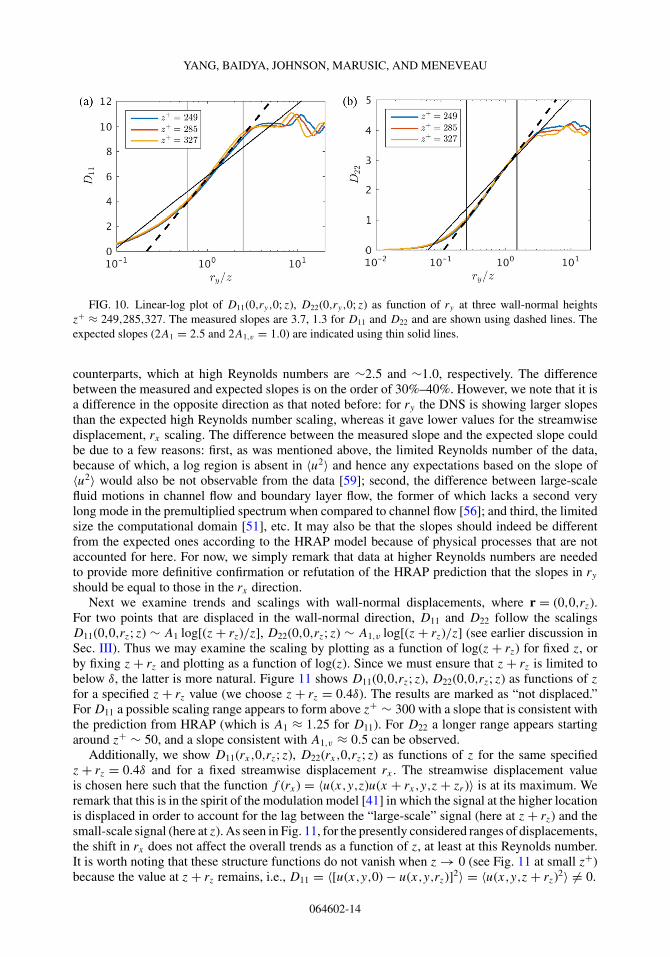
The measured slope for D11(ry) and D22(ry) are, respectively, 3.7 and 1.3. According to HRAP,the expected slopes for the spanwise logarithmic scalings should be the same as their streamwise

064602-13

YANG, BAIDYA, JOHNSON, MARUSIC, AND MENEVEAU

FIG. 10. Linear-log plot of D11(0,ry,0; z), D22(0,ry,0; z) as function of ry at three wall-normal heightsz+ ≈ 249,285,327. The measured slopes are 3.7, 1.3 for D11 and D22 and are shown using dashed lines. Theexpected slopes (2A1 = 2.5 and 2A1,v = 1.0) are indicated using thin solid lines.

counterparts, which at high Reynolds numbers are ∼2.5 and ∼1.0, respectively. The differencebetween the measured and expected slopes is on the order of 30%–40%. However, we note that it isa difference in the opposite direction as that noted before: for ry the DNS is showing larger slopesthan the expected high Reynolds number scaling, whereas it gave lower values for the streamwisedisplacement, rx scaling. The difference between the measured slope and the expected slope couldbe due to a few reasons: first, as was mentioned above, the limited Reynolds number of the data,because of which, a log region is absent in 〈u2〉 and hence any expectations based on the slope of〈u2〉 would also be not observable from the data [59]; second, the difference between large-scalefluid motions in channel flow and boundary layer flow, the former of which lacks a second verylong mode in the premultiplied spectrum when compared to channel flow [56]; and third, the limitedsize the computational domain [51], etc. It may also be that the slopes should indeed be differentfrom the expected ones according to the HRAP model because of physical processes that are notaccounted for here. For now, we simply remark that data at higher Reynolds numbers are neededto provide more definitive confirmation or refutation of the HRAP prediction that the slopes in ry

should be equal to those in the rx direction.Next we examine trends and scalings with wall-normal displacements, where r = (0,0,rz).

For two points that are displaced in the wall-normal direction, D11 and D22 follow the scalingsD11(0,0,rz; z) ∼ A1 log[(z + rz)/z], D22(0,0,rz; z) ∼ A1,v log[(z + rz)/z] (see earlier discussion inSec. III). Thus we may examine the scaling by plotting as a function of log(z + rz) for fixed z, orby fixing z + rz and plotting as a function of log(z). Since we must ensure that z + rz is limited tobelow δ, the latter is more natural. Figure 11 shows D11(0,0,rz; z), D22(0,0,rz; z) as functions of z

for a specified z + rz value (we choose z + rz = 0.4δ). The results are marked as “not displaced.”For D11 a possible scaling range appears to form above z+ ∼ 300 with a slope that is consistent withthe prediction from HRAP (which is A1 ≈ 1.25 for D11). For D22 a longer range appears startingaround z+ ∼ 50, and a slope consistent with A1,v ≈ 0.5 can be observed.

Additionally, we show D11(rx,0,rz; z), D22(rx,0,rz; z) as functions of z for the same specifiedz + rz = 0.4δ and for a fixed streamwise displacement rx . The streamwise displacement valueis chosen here such that the function f (rx) = 〈u(x,y,z)u(x + rx,y,z + zr )〉 is at its maximum. Weremark that this is in the spirit of the modulation model [41] in which the signal at the higher locationis displaced in order to account for the lag between the “large-scale” signal (here at z + rz) and thesmall-scale signal (here at z). As seen in Fig. 11, for the presently considered ranges of displacements,the shift in rx does not affect the overall trends as a function of z, at least at this Reynolds number.It is worth noting that these structure functions do not vanish when z → 0 (see Fig. 11 at small z+)because the value at z + rz remains, i.e., D11 = 〈[u(x,y,0) − u(x,y,rz)]2〉 = 〈u(x,y,z + rz)2〉 �= 0.

064602-14

STRUCTURE FUNCTION TENSOR SCALING IN THE . . .

FIG. 11. Linear-log plot of D11(0,0,rz; z), D22(0,0,rz; z) as functions of z for fixed z + rz = 0.4δ. Theknown slopes A1 ≈ 1.25, A1,v = 0.5 are indicated using dashed lines. We also show results for D11(rx,0,rz; z),and D22(rx,0,rz; z) where rx is such that the function f (rx) = 〈u(x,y,z)u(x + rx,y,z + rz)〉 is at its maximum.Results are denoted as “displaced.”

To observe a logarithmic region, the HRAP formalism requires both z and z + rz to be inthe logarithmic region. This is more easily attained for the spanwise component as 〈vv〉 has anextended logarithmic region, from z+ ≈ 50 to z/δ ≈ 0.4) at this Reynolds number. If we consider〈v2(z)〉 = 〈[v(x,y,z) − 0]2〉 = D22(0,0,rz > δ; z), then in Fig. 11, we are simply taking z + rz fromthe freestream [where v(z + rz) = 0] to a wall-normal location in the boundary layer (z + rz)/δ =0.4. As is seen in Fig. 11(b), this reduces the logarithmic region to a range 50 < z+, z < 0.4(z + rz).The same does not hold for the streamwise component because a logarithmic region can barelybe found in 〈u2〉 at this Reynolds number. So it is interesting that when plotting D11 against z forz + rz = 0.4δ, a logarithmic region begins to emerge, and more so for the displaced data, with theslope close to A = 1.25.

Last we consider structure functions with displacements along a diagonal line on the x-y plane.Figure 12 shows D11, D22 along a sample line that forms a ∼26◦ angle with the x axis (ry/rx = 0.5).As is expected from the HRAP model, logarithmic scalings are still found. Taking a diagonal linemixes the logarithmic scalings in the streamwise and spanwise directions. As a result, from the datathe measured slopes are in between the slopes measured in the spanwise and streamwise directions.Recall that from HRAP the slopes would be expected to be equal for displacements in both directions

FIG. 12. Linear-log plot of D11(rx,ry,0,z), D22(rx,ry,0,z) for ry = rx/2 as a function of r =√

r2x + r2

y at

three wall-normal heights z+ ≈ 249,285,327. The measured slopes are 3.6 and 1.1 for D11 and D22 and areindicated using dashed lines. Logarithmic scalings are observed within the region marked by vertical lines.

064602-15

YANG, BAIDYA, JOHNSON, MARUSIC, AND MENEVEAU

so the differences discussed previously in the context of the spanwise structure functions hold alsofor the present results.

V. CONCLUSIONS

In this work, we investigated the scaling behavior of the full structure function tensor [defined inEq. (1)] in the logarithmic region within the framework provided by the HRAP, which is a simplifiedformalism based on the Townsend attached eddy hypothesis. The results for the required six scalarfunctions as a function of (rx,ry,rz,z) are presented in Eqs. (18), (22), (24), (25), and (27). Certainspecial cases of Eq. (1) have been studied in the past, most notably the streamwise dependencies ofthe streamwise velocity component. In this paper, evidence supporting some of the newly proposedscalings is provided based on hot-wire and DNS data sets, in particular scaling that involves verticaldisplacements with respect to a fixed end point in the bulk region and logarithmic scaling for thetransverse velocity component. However, the slope in the logarithmic laws for structure functionswith displacements in the spanwise directions appeared to be larger than those predicted by thepresent simple version of HRAP. Several additional scalings laws remain to be confirmed in moredetail and in laboratory experiments or DNS, which will need to be at higher Reynolds numbers thanthe ones that are presently available. The modeling work here thus calls for new detailed multipointmeasurements of wall-bounded flows at high Reynolds numbers.

ACKNOWLEDGMENTS

The authors gratefully acknowledge A. Lozano-Duran for making the DNS data set available andfor help accessing it. They acknowledge the financial support of the National Science Foundation,and the Australian Research Council.

[1] A. N. Kolmogorov, The local structure of turbulence in incompressible viscous fluid for very largeReynolds numbers, Dokl. Akad. Nauk SSSR 30, 301-5 (1941).

[2] U. Frisch, Turbulence: The Legacy of A. N. Kolmogorov (Cambridge University Press, Cambridge, 1995).[3] G. E. Karniadakis and K. S. Choi, Mechanisms of transverse motions in turbulent wall flows, Annu. Rev.

Fluid Mech. 35, 45 (2003).[4] A. J. Smits, B. J. McKeon, and I. Marusic, High-Reynolds number wall turbulence, Annu. Rev. Fluid

Mech. 43, 353 (2011).[5] I. Marusic, B. McKeon, P. Monkewitz, H. Nagib, A. Smits, and K. Sreenivasan, Wall-bounded turbulent

flows at high Reynolds numbers: Recent advances and key issues, Phys. Fluids 22, 065103 (2010).[6] A. Townsend, The Structure of Turbulent Shear Flow (Cambridge University Press, Cambridge, 1976).[7] A. E. Perry and I. Marusic, A wall-wake model for the turbulence structure of boundary layers. Part 1.

Extension of the attached eddy hypothesis, J. Fluid Mech. 298, 361 (1995).[8] I. Marusic and A. E. Perry, A wall-wake model for the turbulence structure of boundary layers. Part 2.

Further experimental support, J. Fluid Mech. 298, 389 (1995).[9] T. B. Nickels, I. Marusic, S. Hafez, N. Hutchins, and M. S. Chong, Some predictions of the attached eddy

model for a high Reynolds number boundary layer, Philos. Trans. R. Soc. A 365, 807 (2007).[10] G. L. Eyink, Turbulent flow in pipes and channels as cross-stream “inverse cascades” of vorticity, Phys.

Fluids 20, 125101 (2008).[11] I. Marusic, R. Mathis, and N. Hutchins, Predictive model for wall-bounded turbulent flow, Science 329,

193 (2010).[12] B. McKeon and A. Sharma, A critical-layer framework for turbulent pipe flow, J. Fluid Mech. 658, 336

(2010).[13] V. L. Thomas, B. K. Lieu, M. R. Jovanovic, B. F. Farrell, P. J. Ioannou, and D. F. Gayme, Self-sustaining

turbulence in a restricted nonlinear model of plane couette flow, Phys. Fluids 26, 105112 (2014).

064602-16

STRUCTURE FUNCTION TENSOR SCALING IN THE . . .

[14] J. Bretheim, C. Meneveau, and D. F. Gayme, Standard logarithmic mean velocity distribution in aband-limited restricted nonlinear model of turbulent flow in a half-channel, Phys. Fluids 27, 011702(2015).

[15] M. Hultmark, M. Vallikivi, S. C. C. Bailey, and A. J. Smits, Turbulent Pipe Flow at Extreme ReynoldsNumbers, Phys. Rev. Lett. 108, 094501 (2012).

[16] R. J. Stevens, M. Wilczek, and C. Meneveau, Large-eddy simulation study of the logarithmic law forsecond-and higher-order moments in turbulent wall-bounded flow, J. Fluid Mech. 757, 888 (2014).

[17] K. Talluru, R. Baidya, N. Hutchins, and I. Marusic, Amplitude modulation of all three velocity componentsin turbulent boundary layers, J. Fluid Mech. 746, R1 (2014).

[18] M. Lee and R. D. Moser, Direct numerical simulation of turbulent channel flow up to Reτ ≈ 5200, J. FluidMech. 774, 395 (2015).

[19] G. J. Kunkel and I. Marusic, Study of the near-wall-turbulent region of the high-Reynolds-number boundarylayer using an atmospheric flow, J. Fluid Mech. 548, 375 (2006).

[20] C. de Silva, I. Marusic, J. Woodcock, and C. Meneveau, Scaling of second-and higher-order structurefunctions in turbulent boundary layers, J. Fluid Mech. 769, 654 (2015).

[21] X. I. A. Yang, I. Marusic, and C. Meneveau, Hierarchical random additive process and logarithmic scalingof generalized high-order, two-point correlations in turbulent boundary layer flow, Phys. Rev. Fluids 1,024402 (2016).

[22] T. B. Nickels, I. Marusic, S. Hafez, and M. S. Chong, Evidence of the K−11 Law in a High-Reynolds-Number

Turbulent Boundary Layer, Phys. Rev. Lett. 95, 074501 (2005).[23] C. Meneveau and I. Marusic, Generalized logarithmic law for high-order moments in turbulent boundary

layers, J. Fluid Mech. 719, R1 (2013).[24] A. S. Monin and A. M. Yaglom, Statistical Fluid Mechanics, Volume II: Mechanics of Turbulence (Dover

Publications, Inc., Mineola, NY, 2013).[25] B. Vreman, B. Geurts, and H. Kuerten, Realizability conditions for the turbulent stress tensor in large-eddy

simulation, J. Fluid Mech. 278, 351 (1994).[26] G. L. Eyink and H. Aluie, Localness of energy cascade in hydrodynamic turbulence. I. Smooth coarse

graining, Phys. Fluids 21, 115107 (2009).[27] S. Cerutti and C. Meneveau, Statistics of filtered velocity in grid and wake turbulence, Phys. Fluids 12,

1143 (2000).[28] M. Wilczek, R. J. A. M. Stevens, and C. Meneveau, Spatio-temporal spectra in the logarithmic layer of

wall turbulence: Large-eddy simulations and simple models, J. Fluid Mech. 769, R1 (2015).[29] M. Wilczek, R. J. A. M. Stevens, and C. Meneveau, Height-dependence of spatio-temporal spectra of

wall-bounded turbulence–LES results and model predictions, J. Turbul. 16, 937 (2015).[30] C. Van Atta and W. Chen, Structure functions of turbulence in the atmospheric boundary layer over the

ocean, J. Fluid Mech. 44, 145 (1970).[31] J. C. Kaimal, J. C. Wyngaard, D. A. Haugen, O. R. Coté, Y. Izumi, S. J. Caughey, and C. J. Readings,

Turbulence structure in the convective boundary layer, J. Atmos. Sci. 33, 2152 (1976).[32] P. A. Davidson, T. B. Nickels, and P.-A. Krogstad, The logarithmic structure function law in wall-layer

turbulence, J. Fluid Mech. 550, 51 (2006).[33] R. J. Hill, Exact second-order structure-function relationships, J. Fluid Mech. 468, 317 (2002).[34] A. Cimarelli, E. De Angelis, J. Jimenez, and C. M. Casciola, Cascades and wall-normal fluxes in turbulent

channel flows, J. Fluid Mech. 796, 417 (2016).[35] J. Jiménez, Cascades in wall-bounded turbulence, Annu. Rev. Fluid Mech. 44, 27 (2012).[36] I. Marusic, J. P. Monty, M. Hultmark, and A. J. Smits, On the logarithmic region in wall turbulence,

J. Fluid Mech. 716, R3 (2013).[37] A. E. Perry and M. S. Chong, On the mechanism of wall turbulence, J. Fluid Mech. 119, 173 (1982).[38] J. C. Del Álamo, J. Jimenez, P. Zandonade, and R. D. Moser, Self-similar vortex clusters in the turbulent

logarithmic region, J. Fluid Mech. 561, 329 (2006).[39] J. Woodcock and I. Marusic, The statistical behaviour of attached eddies, Phys. Fluids 27, 015104 (2015).[40] B. Ganapathisubramani, N. Hutchins, J. Monty, D. Chung, and I. Marusic, Amplitude and frequency

modulation in wall turbulence, J. Fluid Mech. 712, 61 (2012).

064602-17

YANG, BAIDYA, JOHNSON, MARUSIC, AND MENEVEAU

[41] R. Mathis, N. Hutchins, and I. Marusic, Large-scale amplitude modulation of the small-scale structures inturbulent boundary layers, J. Fluid Mech. 628, 311 (2009).

[42] R. Mathis, N. Hutchins, and I. Marusic, A predictive inner–outer model for streamwise turbulence statisticsin wall-bounded flows, J. Fluid Mech. 681, 537 (2011).

[43] J. Gärtner, On large deviations from the invariant measure, Theory Probab. Appl. 22, 24 (1977).[44] R. S. Ellis, Large deviations for a general class of random vectors, Ann. Probab. 12, 1 (1984).[45] P. Moin, Revisiting Taylor’s hypothesis, J. Fluid Mech. 640, 1 (2009).[46] C. Geng, G. He, Y. Wang, C. Xu, A. Lozano-Durán, and J. M. Wallace, Taylor’s hypothesis in turbulent

channel flow considered using a transport equation analysis, Phys. Fluids 27, 025111 (2015).[47] J. Kim, P. Moin, and R. Moser, Turbulence statistics in fully developed channel flow at low Reynolds

number, J. Fluid Mech. 177, 133 (1987).[48] R. D. Moser, J. Kim, and N. N. Mansour, Direct numerical simulation of turbulent channel flow up to

Reτ = 590, Phys. Fluids 11, 943 (1999).[49] J. C. Del Alamo, J. Jiménez, P. Zandonade, and R. D. Moser, Scaling of the energy spectra of turbulent

channels, J. Fluid Mech. 500, 135 (2004).[50] S. Hoyas and J. Jiménez, Scaling of the velocity fluctuations in turbulent channels up to Reτ = 2000,

Phys. Fluids 18, 011702 (2006).[51] A. Lozano-Durán and J. Jiménez, Effect of the computational domain on direct simulations of turbulent

channels up to Reτ = 4200, Phys. Fluids 26, 011702 (2014).[52] M. Bernardini, S. Pirozzoli, and P. Orlandi, Velocity statistics in turbulent channel flow up to Reτ = 4000,

J. Fluid Mech. 742, 171 (2014).[53] C. de Silva, D. Krug, D. Lohse, and I. Marusic, Universality of the energy-containing structures in

wall-bounded turbulence, J. Fluid Mech. (unpublished).[54] X. I. A. Yang, C. Meneveau, I. Marusic, and L. Biferale, Extended self-similarity in moment-generating-

functions in wall-bounded turbulence at high Reynolds number, Phys. Rev. Fluids 1, 044405 (2016).[55] N. Hutchins, T. B. Nickels, I. Marusic, and M. S. Chong, Hot-wire spatial resolution issues in wall-bounded

turbulence, J. Fluid Mech. 635, 103 (2009).[56] D. Squire, N. Hutchins, C. Morrill-Winter, M. Schultz, J. Klewicki, and I. Marusic, Applicability of

Taylor’s hypothesis in rough- and smooth-wall boundary layers, J. Fluid Mech. 812, 398 (2017).[57] A. E. Perry, S. Henbest, and M. S. Chong, A theoretical and experimental study of wall turbulence, J.

Fluid Mech. 165, 163 (1986).[58] A. E. Perry and J. D. Li, Experimental support for the attached-eddy hypothesis in zero-pressure-gradient

turbulent boundary layers, J. Fluid Mech. 218, 405 (1990).[59] N. Hutchins and I. Marusic, Large-scale influences in near-wall turbulence, Philos. Trans. R. Soc. A 365,

647 (2007).

064602-18