Structure, dynamics, and robustness of ecological networks
168
Structure, dynamics, and robustness of ecological networks Phillip P.A. Staniczenko Wolfson College University of Oxford A thesis submitted for the degree of Doctor of Philosophy 23rd May, 2011
Transcript of Structure, dynamics, and robustness of ecological networks

Structure, dynamics, and robustness
of ecological networks
Phillip P.A. Staniczenko
Wolfson College
University of Oxford
A thesis submitted for the degree ofDoctor of Philosophy
23rd May, 2011

To My Parents

Structure, dynamics, and robustness of ecological networks
Abstract
Phillip P.A. Staniczenko23rd May, 2011 Clarendon Laboratory
Ecosystems are often made up of interactions between large numbers ofspecies. They are considered complex systems because the behaviour of thesystem as a whole is not always obvious from the properties of the individualparts. A complex system can be represented by a network: a set of intercon-nected objects. In the case of ecological networks and food webs, the objectsare species and the connections are interactions between species. Many com-plex systems are dynamic and exhibit intricate time series. Time series anal-ysis has been developed to understand a wide range of natural phenomena.This thesis deals with the structure, dynamics, and robustness of ecologicalnetworks, the spatial dynamics of fluctuations in a social system, and theanalysis of cardiac time series. Biodiversity on Earth is decreasing largelydue to human-induced causes. My work looks at the effect of anthropogenicchange on ecological networks. In Chapter Two, I investigate predator adap-tation on food-web robustness following species extinctions. I identify anew theoretical category of species that may buffer ecosystems against en-vironmental change. In Chapter Three, I study changes in parasitoid-host(consumer-resource) interaction frequencies between complex and simple en-vironments. I show that the feeding preferences of parasitoid species activelychange in response to habitat modification. Ecological networks are embed-ded in spatially-heterogeneous landscapes. In Chapter Four, I assess the roleof geography on population fluctuations in an analogous social system. Idemonstrate that fluctuations in the number of venture capital firms regis-tered in cities in the United States of America are consistent with spatial andtemporal contagion. Understanding how physiological signals vary throughtime is of interest to medical practitioners. In Chapter Five, I present atechnique for quickly quantifying disorder in high frequency event series.Applying the algorithm to patient cardiac time series provides a rapid wayto detect the onset of heart arrhythmia. Increasingly, answers to scientificquestions lie at the intersection of traditional disciplines. This thesis appliestechniques developed in physics and mathematics to problems in ecology andmedicine.
i

Preface
This thesis describes work carried out at the Clarendon Laboratory in Ox-ford between October 2007 and September 2010. I am the recipient of adoctoral studentship in Complex Systems and Networks Research from theCentre of Excellence in Computational Complex Systems Research (HelsinkiUniversity of Technology). I am affiliated with the Department of Physicsand the Cabdyn Complexity Centre (Saıd Business School).
This thesis is entirely my own work, and except where otherwise stated, de-scribes my own research. Two chapters have been published and two chaptersare in preparation for submission to peer-review journals.
• Chapter 2: Staniczenko, P.P.A., Lewis, O.T., Jones, N.S. & Reed-Tsochas, F.(2010). Structural dynamics and robustness of food webs. Ecology Letters, 13,891-899.
• Chapter 3: Staniczenko, P.P.A., Lewis, O.T., Tylianakis, J.M., Albrecht, M.,Klein, A.-M., Gathmann, A. & Reed-Tsochas, F. (2010). Active reallocation offood-web interactions under environmental change, in preparation.
• Chapter 4: Staniczenko, P.P.A., Reed-Tsochas, F., Plant, R.T. & Johnson, N.F.(2010). Spatial contagion of fluctuations in social systems, in preparation.
• Chapter 5: Staniczenko, P.P.A., Lee, C.-F. & Jones, N.S. (2009). Rapidly de-tecting disorder in rhythmic biological signals. Physical Review E, 79:011915.Copyright (2009) by the American Physical Society.
I was responsible for all analysis and writing. The following authors kindlyprovided their data: JMT, MA, AMK, AG, and RTP. All authors discussedthe results and edited the relevant manuscripts.
I am grateful for the input from my collaborators; I extend special thanksto Felix Reed-Tsochas, Owen Lewis, Jennifer Dunne, Nick Jones, and NeilJohnson for their guidance and support. I am indebted to my family andfriends, many of whom will never read this thesis; however, this work wouldnot exist without them.
ii

Contents
Abstract i
Preface ii
1 Introduction 1
2 Structural dynamics and robustness of food webs 25
2.1 Introduction . . . . . . . . . . . . . . . . . . . . . . . . . . . . 262.2 Materials and Methods . . . . . . . . . . . . . . . . . . . . . . 292.3 Results . . . . . . . . . . . . . . . . . . . . . . . . . . . . . . . 352.4 Discussion . . . . . . . . . . . . . . . . . . . . . . . . . . . . . 40
3 Active reallocation of food-web interactions under environ-
mental change 53
3.1 Introduction . . . . . . . . . . . . . . . . . . . . . . . . . . . . 543.2 Materials and Methods . . . . . . . . . . . . . . . . . . . . . . 563.3 Results . . . . . . . . . . . . . . . . . . . . . . . . . . . . . . . 653.4 Discussion . . . . . . . . . . . . . . . . . . . . . . . . . . . . . 713.5 Appendix . . . . . . . . . . . . . . . . . . . . . . . . . . . . . 80
3.5.1 Quantitative food-web metrics . . . . . . . . . . . . . . 803.5.2 Active reallocation model . . . . . . . . . . . . . . . . 81
4 Spatial contagion of fluctuations in social systems 83
4.1 Introduction . . . . . . . . . . . . . . . . . . . . . . . . . . . . 844.2 Model and methods . . . . . . . . . . . . . . . . . . . . . . . . 864.3 Results . . . . . . . . . . . . . . . . . . . . . . . . . . . . . . . 914.4 Discussion . . . . . . . . . . . . . . . . . . . . . . . . . . . . . 934.5 Appendix . . . . . . . . . . . . . . . . . . . . . . . . . . . . . 102
4.5.1 Empirical data . . . . . . . . . . . . . . . . . . . . . . 1024.5.2 Results for 7 additional regions . . . . . . . . . . . . . 104
iii

5 Rapidly detecting disorder in rhythmic biological signals 113
5.1 Introduction . . . . . . . . . . . . . . . . . . . . . . . . . . . . 1145.2 Data Analysis . . . . . . . . . . . . . . . . . . . . . . . . . . . 116
5.2.1 Symbolizing cardiac data . . . . . . . . . . . . . . . . . 1175.2.2 Spectral entropy . . . . . . . . . . . . . . . . . . . . . 1175.2.3 Parameter selection . . . . . . . . . . . . . . . . . . . . 1225.2.4 Cardiac disorder map . . . . . . . . . . . . . . . . . . . 126
5.3 Algorithm . . . . . . . . . . . . . . . . . . . . . . . . . . . . . 1305.3.1 Arrhythmia detection algorithm . . . . . . . . . . . . . 1305.3.2 Algorithm results . . . . . . . . . . . . . . . . . . . . . 132
5.4 Discussion . . . . . . . . . . . . . . . . . . . . . . . . . . . . . 1355.4.1 Disagreements with annotations . . . . . . . . . . . . . 1365.4.2 Other rhythms . . . . . . . . . . . . . . . . . . . . . . 1385.4.3 Comparison to other methods . . . . . . . . . . . . . . 1405.4.4 Systematic error . . . . . . . . . . . . . . . . . . . . . 141
5.5 Further Work . . . . . . . . . . . . . . . . . . . . . . . . . . . 1425.6 Conclusion . . . . . . . . . . . . . . . . . . . . . . . . . . . . . 1435.7 Appendix . . . . . . . . . . . . . . . . . . . . . . . . . . . . . 151
5.7.1 Disagreements with annotations . . . . . . . . . . . . . 1515.7.2 Other rhythms . . . . . . . . . . . . . . . . . . . . . . 154
Conclusion 156
iv

List of Tables
2.1 Structural properties of food webs and simulation results . . . 30
3.1 Food-web descriptions and model parameters . . . . . . . . . . 583.2 Empirical food-web metric values and model results . . . . . . 59
4.1 Results for 9 US regions . . . . . . . . . . . . . . . . . . . . . 90
5.1 Summary of arrhythmia detection algorithm symbols . . . . . 1185.2 Results of the arrhythmia detection algorithm . . . . . . . . . 1345.3 Summary of results for variance windows of different lengths . 135
v

List of Figures
1.1 Our New Age by Athelstan Spilhaus . . . . . . . . . . . . . . 14
2.1 Predator-prey rewiring model . . . . . . . . . . . . . . . . . . 322.2 Secondary extinction sequences for 12 food webs . . . . . . . . 372.3 Proportional increase in robustness and overlap species . . . . 38
3.1 Switzerland food web in complex and simple environments . . 603.2 Parasitoid interaction generality in simple environments . . . . 663.3 Interaction generality and z-score . . . . . . . . . . . . . . . . 673.4 Active reallocation model parameter space for Ecuador . . . . 693.5 Active reallocation model parameter space for Germany . . . . 703.6 Active reallocation model parameter space for Indonesia . . . 703.7 Active reallocation model parameter space for Switzerland . . 713.8 Model closeness values for four regions . . . . . . . . . . . . . 72
4.1 Histogram of VCF density for US 509 cities . . . . . . . . . . 914.2 Fluctuations and VCF density . . . . . . . . . . . . . . . . . . 924.3 Fluctuation patterns in California North and Massachusetts
state . . . . . . . . . . . . . . . . . . . . . . . . . . . . . . . . 944.4 City influence network composition for California North and
Massachusetts state . . . . . . . . . . . . . . . . . . . . . . . . 954.5 Influence network topology at the critical inter-city influence
distance for California North and Massachusetts state . . . . . 964.6 Fluctuation patterns in California South . . . . . . . . . . . . 1064.7 Fluctuation patterns in Connecticut . . . . . . . . . . . . . . . 1074.8 Fluctuation patterns in New Jersey . . . . . . . . . . . . . . . 1084.9 Fluctuation patterns in New York State . . . . . . . . . . . . 1094.10 Fluctuation patterns in Pennsylvania . . . . . . . . . . . . . . 1104.11 Fluctuation patterns in Texas . . . . . . . . . . . . . . . . . . 1114.12 Fluctuation patterns in Virginia . . . . . . . . . . . . . . . . . 112
5.1 Arrhythmia Detection Algorithm Schematic . . . . . . . . . . 119
vi

5.2 Spectral entropy for Patient 08378 . . . . . . . . . . . . . . . . 1255.3 Cardiac Disorder Map . . . . . . . . . . . . . . . . . . . . . . 1275.4 Patient 08219, 11 880 s, missed atrial fibrillation . . . . . . . . 1525.5 Patient 08434, 9504 s, missed atrial fibrillation . . . . . . . . . 1525.6 Patient 04936, 7347 s, missed atrial flutter . . . . . . . . . . . 1535.7 Patient 08219, 10 090 s, missed atrial flutter . . . . . . . . . . 1535.8 Patient 04936, 17 785 s, fib-flutter . . . . . . . . . . . . . . . . 1545.9 Patient 04936, 18 440 s, fib-flutter . . . . . . . . . . . . . . . . 1555.10 Patient 05901, 6714 s, sinus arrest . . . . . . . . . . . . . . . . 155
vii

“What we observe is not nature itself, but nature exposed to our methods of
questioning.”
Werner Heisenberg in Physics and Philosophy (1958)

Chapter 1
Introduction
Ecosystems are often made up of interactions between large numbers of
species. They are considered complex systems because the behaviour of the
system as a whole is not always obvious from the properties of the individ-
ual parts. A complex system can be represented by a network: a set of
interconnected objects. In the case of ecological networks, the objects are
species and the connections are interactions between species. Work on the
structure of complex systems and networks (Newman 2003) has drawn on
methods developed in condensed matter physics, such as statistical mechan-
ics, quantum mechanics and field theory (Albert & Barabasi 2002). Many
complex systems are dynamic and exhibit intricate time series (Boccaletti et
al. 2006; Barrat et al. 2008). This thesis deals with the structure, dynamics,
and robustness of ecological systems (Chapters Two and Three), the spatial
dynamics of fluctuations in a social system (Chapter Four), and the analysis
of cardiac time series (Chapter Five).
In a network, objects are called nodes or vertices, and the connections
between objects are called links or edges. Properties of these abstract sys-
tems have been studied by mathematicians since the 1950s in the field of
1

graph theory (Erdos & Renyi 1959; Bollobas 2001). An example of a real
network is a social one: humans are represented by nodes and are connected
to acquaintances by links. In 1967, Milgram published the findings of his
famous “six degrees of separation” letter forwarding experiment (Miligram
1967). He showed that the average (shortest) number of links between in-
dividuals was smaller than previously expected. This became known as the
“small-world” effect (Watts & Strogatz 1998).
Advances in the theory of networks have been driven by the availability
of data (Newman et al. 2006). Theory is developed to understand a wide
range of empirical systems. Examples of biological systems include metabolic
networks, protein-protein interaction networks, and neural networks (ibid).
Examples of technological systems include the internet, the world wide web,
and product supply-chains (ibid). Examples of social systems include friend-
ship networks, disease spread on human-contact networks, and networks of
inter-bank loans (ibid).
The structure of empirical networks often change thorough time (Doro-
govtsev & Mendes 2002). Work to date has focused on growing networks:
where the number of nodes and links increases through time. This is largely
due to lack of data on networks that are decreasing in size. Only recently
have contracting networks been considered (Saavedra et al. 2008).
Ecological networks comprise many complex interactions between species
(Pascual & Dunne 2006). Biodiversity on Earth is decreasing and ecological
networks are losing species, largely due to human-induced causes (Millennium
Ecosystem Assessment 2005). My work seeks to understand the effects of
anthropogenic change on the structure and dynamics of ecological networks.
2

In Chapter Two, I investigate predator adaptation on food-web robustness
following species extinction. In Chapter Three, I study changes in parasitoid-
host (consumer-resource) interaction frequencies between complex and simple
environments. Ecological networks are embedded in spatially-heterogeneous
landscapes. In Chapter Four, I assess the role of geography on population
fluctuations in an analogous social system: the number of venture capital
firms registered in cities in the United States of America (US) between 1981
and 2003.
Time series analysis has been developed to investigate a wide range of nat-
ural phenomena (Kantz & Schreiber 2003). Understanding how physiological
signals vary through time is of interest to medical practitioners (Richman &
Moorman 2000). In particular, the study of electrocardiograms has lead to
significant improvements in patient care (Braunwald 1997).
In Chapter Five, I present a technique for quickly quantifying disorder in
high frequency event series (published, Staniczenko et al. 2009). The method
uses changes in frequency-domain entropy to identify periods of irregular
rhythm. I use this method to distinguish two forms of cardiac arrhythmia—
atrial fibrillation and atrial flutter—from normal sinus rhythm. Applying the
algorithm to patient data provides a rapid way to detect arrhythmia, demon-
strating usable response times as low as six seconds (with correct assessment
of 85.7% of professional beat-classifications).
Statistical approaches have required around two minutes to detect changes
in rhythm (Tateno & Glass 2000; Sarkar et al. 2008). By contrast, the
entropy-based method is applicable to short sections of data, enabling quicker
response times. Combination of these approaches is desirable in an automatic
3

detector of arrhythmia. Such a detector would be clinically useful in mon-
itoring for relapse of fibrillation in patients and in assessing the efficacy of
anti-arrhythmic drugs (Israel 2004).
Theoretical ecology, unlike other natural sciences, has no widely accepted
first-principle laws such as gravity, conservation of mass, or inheritance. Dif-
ferent theories and models must be invoked to answer the questions posed
in population, community and conservation ecology. Nevertheless, ecological
theory has a unifying intention: as Ilkka Hanski (1999) writes, “Mathematical
models [. . . ] are constructed in the hope that they will clarify our thinking,
reveal unexpected and significant consequences of particular assumptions,
and lead to interesting new predictions that could be tested with observa-
tional and experimental studies.”
A central goal of ecological research is to understand the mechanisms
influencing the persistence of ecosystems. Studies of the complex interactions
between species (Darwin 1859; Hutchinson 1957) have played a significant
role in the development of ecology as a scientific discipline (Hardy 1924;
Elton 1927). The approach of population and community ecology (following
Elton 1927; MacArthur 1955) considers individual species as the fundamental
unit of study. Interactions between species can be formulated in terms of
ecological networks (Montoya et al. 2006). Networks may comprise species
and interaction presence-absence data (binary), or contain information on
species abundances and interaction strengths (weighted).
Natural ecosystems comprise a range of interactions. But research to date
typically distinguishes between three types of network (Ings et al. 2009): (i)
predator-prey food-webs; (ii) parasitoid-host webs; and (iii) mutualistic webs.
4

Predator-prey and parasitoid-host webs describe antagonistic relationships
between species, while species in the mutualistic web benefit from interacting.
The impact of anthropogenic environmental change (e.g., Sala 2000) has
motivated studies of the stability and robustness of ecological networks. This
is because the communities of species described by ecological networks often
provide ecosystem services that are of great practical benefit to humankind
(Costanza et al. 1997).
Seminal work by Robert May (1972) used random matrix theory to assess
the stability of random assemblages of interacting species to perturbation. He
found that increasing interaction complexity led to reduced system stability.
This relationship questioned the observation that empirical data repeatedly
demonstrated the prevalence of complexity in nature (Polis 1991; Williams
& Martinez 2000). One possible explanation for this difference is May’s
assumption of random interactions: the structure of empirical networks was
subsequently shown to follow non-random distributions (Dunne et al. 2002a).
Structural food-web research has received renewed interest following a
series of highly critical reviews in the late 1980s and early 1990s (Paine
1988; Hall & Raffaelli 1993). This may be attributable to the collection of
improved empirical food-webs as well as an influx of new analytical methods
from other disciplines. Studies of biological, technological and social networks
have provided new ideas and new perspectives from which to study ecological
networks (Proulx et al. 2005).
Of the different types of ecological network, predator-prey food-webs have
received the most attention during the early development of the field (Pimm
1982; Cohen et al. 1993). The current “second-generation” empirical food
5

webs (see Allesina & Pascual 2009 for a collection) have been thoroughly
studied with respect to their structural properties and theoretical robustness
to secondary extinctions (summarised in Pascual & Dunne 2006). One study
(Dunne et al. 2002b) found that robustness increases with connectance (a
structural measure of food-web complexity), in direct contrast to the finding
of May. Modelling secondary extinctions has informed structural traits that
may identify keystone species: typically understood as a species that has a
disproportionate effect on its environment relative to its biomass (introduced
in Paine 1969, review in Mills et al. 1993). The identification and study of
keystone species is important in conservation ecology (ibid).
Robustness studies to date have only considered static food-web struc-
tures (but see Kaiser-Bunbury et al. 2010). This is despite the widely held
view that there are many possible types of compensatory dynamics in ecosys-
tems that may alter food-web structure (e.g., Brown et al. 2001). Indeed,
in Jennifer Dunne’s study (Dunne et al. 2002b) of food-web robustness she
writes, “. . . our simple algorithm for generating secondary extinctions is lim-
ited, and may overestimate secondary extinctions since species can survive
by switching to less preferred prey.”
In Chapter Two, I present a model that introduces structural dynamics
into the framework of secondary-extinction robustness analysis (published,
Staniczenko et al. 2010a). In the model, trophic links may be rewired follow-
ing the loss of a predator species from the food web. Due to reduced competi-
tion, species loosing a predator become more available to other, biologically-
plausible, predators. I compare the increase in robustness conferred through
rewiring in 12 empirical food webs. Using the model, I identify a new theo-
6
retical category of species—overlap species—which promote adaptive robust-
ness. These findings underline the importance of compensatory mechanisms
that may buffer ecosystems against environmental change, and highlight the
likely role of particular species that are expected to facilitate this buffering.
The introduction of structural dynamics represents a significant advance
in the theoretical treatment of food-web robustness. The method may be in-
corporated into other theoretical frameworks (e.g., population dynamics), ex-
tending the realism of community-level models. The identification of overlap
species raises important practical questions in conservation biology. Which
species in an ecosystem enable adaptation and hence additional robustness?
What mechanisms underlie this form of adaptation? And what is the rela-
tionship, perhaps phylogenetic, between these species? Thus, in complement
to keystone species, whose removal causes large cascading effects, we must
ask: which species provide ecosystem stability in the first place? In addition
to protecting keystone species, conservationists must preserve the diversity
of overlap species in order to maintain functional ecosystems.
Models that aim to describe the structure of food webs typically fall into
two broad categories (Stouffer 2010): (i) phenomenological models and (ii)
population-level models. Phenomenological models rely on heuristic rules to
determine how species select their prey and thus generate food-web structure
(Cohen & Newman 1985; Williams & Martinez 2000; Cattin et al. 2004).
Population-level models prescribe an ecologically-motivated generative mech-
anism and resulting interactions produce food-web structure (e.g., Loeuille
& Loreau 2005). Mechanistic models based on first principles are generally
preferred to phenomenological models due to their inherent predictive, rather
7
than pattern-fitting, nature (Ings et al. 2009).
Recent work by Beckerman, Petchey & Warren (2006) used foraging the-
ory (MacArthur & Pianka 1966; Pulliam 1974; Stephens & Krebs 1986) as an
ecological basis to determine some emergent properties (e.g., connectance) of
food-web structure. This work was then extended to include species allome-
tries (body-size) to predict interactions observed in empirical predator-prey
food webs (Petchey et al. 2008; but see Allesina 2010). However, these mech-
anistic models are currently limited to size-structured, binary, food-webs.
It is well known that not all species and interactions are equally important
(Paine 1980; Benke & Wallace 1997). The prevalence of weak interactions
in nature (Berlow et al. 1999) has cast new light on the complexity-stability
debate (Polis 1998; McCann 2000). Several key studies (Paine 1992; McCann
et al. 1998) suggested that weak links tended to stabilise local community
dynamics. The advent of increasingly quantified webs (e.g., Muller et al.
1999) has enabled more rigorous testing of the role interaction strength plays
in determining food-web stability. It has been shown that the configuration
of weak and strong links, not just the presence of weak links, has implications
for ecosystem functionality (Bascompte et al. 2005, 2006).
Methods summarising the information contained in quantitative webs
(Bersier et al. 2002) has facilitated detailed studies of the effects of habitat
modification on species interaction patterns (Klein et al. 2006; Tylianakis
et al. 2007; Albrecht et al. 2007). Across these distinct studies, struc-
tural metrics describing parasitoid-host webs were observed to change with
similar pattern along increasing land-use gradients. However, the mecha-
nisms responsible for these structural changes are unknown. One study of
8

host-parasite1 interactions suggested that observed topological patterns arise
from species abundance distributions (Vazquez et al. 2005, 2007).
In Chapter Three, I show that the feeding preferences of consumer species
can actively change in response to habitat modification (in preparation, Stan-
iczenko et al. 2010b). Parasitoid species focused on particular trophic inter-
actions within their existing set. Their distribution of interactions differed
significantly from what would be expected if density-dependent reallocation
is assumed. I present a model of consumer feeding reallocation that gener-
ates quantitative food webs in simplified environments and test the model
against empirical data. I show that consumer preference for resource species
can alter between environments, resulting in corresponding changes to the
structural properties of their community food webs. My findings suggest that
in environments where communities are more impacted by habitat modifi-
cation, interaction patterns will increasingly depart from density-dependent
resource selection.
The active reallocation model is able to generate quantitative interaction
frequencies in non-size-structured food webs. This represents a large step
forward in modelling realistic consumer feeding behaviour. Since parasitoids
are natural enemies of many crop pests (Hawkins 1994), knowledge of altered
interaction pattern in modified environments could be exploited to control
outbreaks of previously less abundant pests. Understanding the mechanisms
underlying species interactions subject to environmental change will help
with the planning of habitat restoration and with assessing its efficacy. Active
1Parasites are distinguished from parasitoids in that a parasitoid ultimately causes thedeath of its host organism.
9

reallocation is a significant and functionally important process that needs to
be taken into account when developing forecasts of the effects of human-
induced disturbances on community structure and composition.
I argue that active reallocation is consistent with differences in parasitoid
foraging behaviour between forested and unforested habitats (Laliberte &
Tylianakis 2010). This suggests that foraging behaviour is a strong can-
didate for the ecological mechanism causing structural differences between
quantitative webs. Not unsurprisingly, the environment in which a species
is located has direct influence on its foraging behaviour. This explains the
variable trophic breadths of parasitoid species observed in empirical data.
The traditional approach to population ecology assumes that individuals
in a (species) population share the same environment (Kingland 1985; McIn-
tosh 1985). However, populations are often non-homogenously distributed
throughout the spatial landscape (Turner 1989; Wiens 1997). Metapopula-
tion ecology provides an explicit treatment of space within its conceptual
framework (Hanski 1999).2 Hanski (ibid) describes metapopulation stud-
ies as “typically assum[ing] an environment consisting of discrete patches of
suitable habitat surrounded by uniformly unsuitable habitat.”
Metapopulation ecology is primarily concerned with the density of pop-
ulations within patches and the emigration and immigration of populations
between patches (Levin et al. 1993). Metapopulation theory, along with
population ecology in the wider sense, is often restricted by the large scale
of the study phenomena required to test model predictions (Hassell et al.
2There are two other approaches to large-scale spatial ecology: landscape ecology andspatial dynamics in continuous space (Hanski 1999 pp3-4).
10

1989). Lack of extensive field studies has hampered progress in refining
models dealing with fragmented landscapes. This is despite growing evi-
dence linking species extinction to habitat fragmentation (e.g., Pimm 1998).
Although large-scale population data is sparse, field studies have provided
some evidence in support of metapopulation dynamics. Notably: population
density is significantly affected by patch area and isolation (Turner 1989;
Wiens 1997) and migration and immigration (Krebs 1994).
Spatial synchrony refers to coincident changes in the time-varying char-
acteristics of geographically separated populations (see Liebhold et al. 2004
for a review). The concept of population synchrony is particularly relevant
to metapopulation systems because synchrony is directly related to the like-
lihood of global extinction (Heino et al. 1997). Synchrony is typically mea-
sured by correlation in abundance and many studies found that synchrony
declines as the distance separating populations increases (ibid). Due to dif-
ficulty collecting extensive spatiotemporal ecological data, metapopulation
and population dynamics studies have focused on spatial correlations of pop-
ulation density in fragmented landscapes. The dynamics of fluctuations in
species populations has received little or no attention.
Within metapopulation ecology (and population ecology more generally),
fluctuations in population have two important consequences: (i) positive
fluctuations can lead to local population outbreaks and (ii) negative fluctua-
tions can lead to local population extinctions. Studies relating heterogeneous
spatial landscapes to synchronous population extinctions have been almost
exclusively theoretical (Liebhold et al. 2004). A prototypical example is
the study by Earn et al. (2000) in which the authors used a simple spatial
11

population model to assess the influence of “conservation corridors” on pop-
ulation synchronicity. In this and similar studies, the aim was to understand
the analytical relationship between mathematical parameters governing syn-
chronicity and fluctuations leading to local, and ultimately global, extinc-
tions. A systemic study of the spatial-temporal patterns of fluctuations has,
to my knowledge, yet to be studied.
In Chapter Four, I analyse the spatial and temporal pattern of fluctua-
tions in the number of venture capital firms (VCFs) registered in US cities
(in preparation, Staniczenko et al. 2010c). Data comprise the number of reg-
istered VCFs in 509 cities (VCF populations) sampled yearly over the period
1981 to 2003. I argue that VCF dynamics, in addition to being of interest to
the social sciences, has implications for spatial ecology where suitable data
are less available for analysis. In the metapopulation-analogous framework
of cities (patches) non-homogenously distributed through US states, I show
that fluctuations in VCF populations are consistent with spatial contagion.
That is, fluctuations in a city are more likely to occur if neighbouring cities
demonstrated fluctuations during the preceding year.
To describe the observed VCF fluctuation dynamics, I propose a model
that posits three phenomenological features: (i) cities strongly induce self-
fluctuations; (ii) the (fluctuation) influence of cities on proximate cities fol-
lows an exponentially-decaying function; and (iii) the influence of proximate
cities on the fluctuation behaviour of a city is cumulative. The model pro-
vides a good fit to the empirical data compared to two null models. One null
model assumes fluctuations are independent of city identity and geographi-
cal location; the other null model incorporates the empirical observation that
12

some cities experience greater numbers of fluctuations than others.
Although the study in Chapter Four involves populations of VCFs, the
findings have direct relevance to problems in spatial ecology. Primarily: are
fluctuations in local species abundance spatially contagious? A more thor-
ough investigation of population synchronicity, beyond simple density effects,
may lead to more effective methods to control or eradicate invasive species.
Furthermore, the simple model of spatial contagion can be used to improve
our understanding of the effects of habitat fragmentation—patches of land
joined by conservation corridors—on metapopulation persistence.
Ecological theory, in turn, may provide candidate mechanisms for the
phenomena observed in the VCF data. Four areas of the population syn-
chrony literature motivated my explanation of VCF fluctuation dynamics:
(i) observed patterns in the dispersal of species populations; (ii) impact of
habitat quality on population density; (iii) synchronicity of population den-
sity with exogenous factors; and (iv) focal species’ interactions with other
species populations demonstrating synchrony. Indeed, the social sciences
have drawn greatly on ecology: not least in organisational ecology. Insights
from ecology and biology have been combined with economics and sociology
to understand the conditions under which organisations emerge, grow and
die (Hannan & Freeman 1977, 1989).
The theme of this Introduction has been the interplay of theory and data.
From this interplay emerge phenomenological and mechanistic descriptions of
the natural world. The success of ecology, as with all the natural sciences, re-
lies on the work of both experimentalists and theoreticians. As we experience
rapid environmental change, the questions asked in ecology are becoming in-
13

creasingly important. The methods used to find answers and solutions may
improve, but the fundamental goal remains the same: as Athelstan Spilhaus
wrote, “[Ecological] models as they develop will not only provide understand-
ing, but also when we build a highway, dam, city or pipeline—predict the
consequences!”
Figure 1.1: Our New Age by Athelstan Spilhaus, circa 1950.
References
Albert, R. & Barabasi, A.-L. (2002). Statistical mechanics of complex net-
works. Rev. Mod. Phys., 74, 47–97.
Albrecht, M., Duelli, P., Schmid, B. & Muller, C.B. (2007). Interaction diver-
sity within quantified insect food webs in restored and adjacent intensively
managed meadows. J. Anim. Ecol., 76, 1015–1025.
14

Allesina, S. & Pascual, M. (2009). Googling food webs: can an eigenvec-
tor measure species’ importance for coextinctions? PLoS. Comp. Biol., 5,
e1000494.
Allesina, S. (2010). Predicting trophic relations in ecological networks: A
test of the allometric diet breadth model. J. Theor. Biol., doi:10.1016/
j.jtbi.2010.06.040.
Barrat, A., Barthelemy, M. & Vespignani, A. (2008). Dynamical Processes
on Complex Networks. Cambridge University Press, Cambridge, UK.
Bascompte, J., Melian, C.J. & Sala, E. (2005). Interaction strength com-
binations and the overfishing of marine food web. Proc. Natl. Acad. Sci.
USA, 102, 5443-5447.
Bascompte, J., Jordano, P. & Olesen, J.M. (2006). Asymmetric coevolution-
ary networks facilitate biodiversity maintenance. Science, 312, 431-433.
Beckerman, A.P., Petchey, O.L. & Warren, P.H. (2006). Foraging biology
predicts food web complexity. Proc. Natl. Acad. Sci. USA, 103, 13 745-
13 749.
Benke, A.C. & Wallace, J.B. (1997). Trophic basis of production among
riverine caddisflies: implications for food web analysis. Ecology, 78, 1132-
1145.
Berlow, E.L. (1999). Strong effects of weak interactions in ecological com-
munities. Nature, 398, 330-333.
15

Bersier, L.-F., Banasek-Richter, C. & Cattin, M.F. (2002). Quantitative
descriptors of food-web matrices. Ecology, 83, 2394–2407.
Boccaletti, S., Latora, V., Moreno, Y., Chavez, M. & Hwang, D.-U. (2006).
Complex networks: Structure and Dynamics. Physics Reports, 424, 175–308.
Bollobas, B. (2001). Random Graphs, 2nd Edition. Cambridge University
Press, Cambridge, UK.
Braunwald, E. (Editor) (1997). Heart Disease: A Textbook of Cardiovascular
Medicine, Fifth Edition. W.B. Saunders Co., Philadelphia, PA, pp 108.
Brown, J.H., Whitham, T.G., Morgan Ernest, S.K. & Gerhring, C.A. (2001).
Complex species interactions and the dynamics of ecological systems: long-
term experiments. Science, 293, 643–650.
Cattin, M.F., Bersier, L.-F., Banasek-Richter, C., Baltensperger, R. & Gabriel,
J.P. (2004). Phylogenetic constraints and adaptation explain food-web struc-
ture. Nature, 427, 835-839.
Cohen, J.E. et al. (1993). Improving food webs. Ecology, 74, 252–258.
Cohen, J.E. & Newman, C.M. (1985). A stochastic theory of community
food webs: Models and aggregated data. Proc. R. Soc. B, 224, 421-448.
Costanza, R. et al. 1997. The value of the world’s ecosystem services and
natural capital. Nature, 387, 253–260.
Darwin, C. (1859). On the Origin of Species by Means of Natural Selection,
16

or the Preservation of Favoured Races in the Struggle for Life. John Murray,
London, UK.
Dorogovtsev, S.N. & Mendes, J.F.F. (2002). Evolution of networks. Adv.
Phys., 51, 1079–1187.
Dunne, J.A., Williams, R.J. & Martinez, N.D. (2002a). Food-web structure
and network theory: the role of connectance and size. Proc. Natl. Acad.
Sci. USA, 99, 12 917-12 922.
Dunne, J.A., Williams, R.J. & Martinez, N.D. (2002b). Network structure
and biodiversity loss in food webs: robustness increases with connectance.
Ecol. Lett., 5, 558–567.
Earn D.J.D., Levin, S.A. & Rohani, P. (2000). Coherence and conservation.
Science, 290, 1360–1364.
Elton, C.S. (1927). Animal Ecology. Sedgewick and Jackson, London, UK.
Erdos, P. & Renyi, A. (1959). On random graphs 1. Publ. Math. Debrecen.,
6, 290–297.
Hall, S.J. & Raffaelli, D.G. (1993). Food webs–theory and reality. Adv. Ecol.
Res., 24, 187-239.
Hannan, M.T. & Freeman, J. (1977). The population ecology of organiza-
tions. Am. J. Sociol., 82, 929–964.
Hannan, M.T. & Freeman, J. (1989). Organization Ecology. Harvard Uni-
17

versity Press, Cambridge, MA.
Hanski, I. (1999). Metapopulation Ecology. Oxford University Press, USA,
pp. 11–13.
Hardy, A.C. (1924). The Herring in Relation to its Animate Environment,
Part 1. Ministry of Agriculture and Fisheries, London, UK.
Hassel, M.P., Latto, J. & May, R.M. (1989). Seeing the wood for the trees:
detecting density dependence from existing life-table studies. J. Anim. Ecol.,
58, 883–892.
Hawkins, B.A. (1994). Pattern and Process in Host-parasitoid Interactions.
Cambridge University Press, Cambridge, UK.
Heino, M., Kaitala, V., Ranta, E. & Lindstrom, J. (1997). Synchronous
dynamics and rates of extinction in spatially structured populations. Proc.
R. Soc. B, 264, 481–486.
Hutchinson, G.E. (1957). Concluding remarks. Cold Spring Harb. Symp.
Quant. Biol., 22, 415–427.
Ings, T.C. et al. (2009). Ecological networks—beyond food webs. J. Anim.
Ecol., 78, 253–269.
Israel, C.W., Gronefeld, G., Ehrlich, J.R., Li, Y.-G. & Hohnloser, S.H.
(2004). Long-term risk of recurrent atrial fibrillation as documented by an
implantable monitoring device. J. Am. Coll. Cardiol., 43, 47–52.
18

Kaiser-Bunbury, C.N., Muff, S., Memmott,J., Mller C.B. & Caflisch, A.
(2010). The robustness of pollination networks to the loss of species and in-
teractions: a quantitative approach incorporating pollinator behaviour. Ecol.
Lett., 13, 442–452.
Kantz, H. & Schreiber, T. (2003). Nonlinear Time Series Analysis. Cam-
bridge University Press, Cambridge, UK.
Kingland, S. (1985). Modeling Nature. Chicago University Press, Chicago,
Il.
Klein, A.M., Steffan-Dewenter, I. & Tscharntke, T. (2006). Rain forest pro-
motes trophic interactions and diversity of trap-nesting Hymenoptera in ad-
jacent agroforestry. J. Anim. Ecol., 75, 315–323.
Krebs, C.J. (1994). The Experimental Analysis of Distribution and Abun-
dance. Harper & Row, New York, NY.
Laliberte, E. & Tylianakis, J.M. (2010). Deforestation homogenizes tropical
parasitoid-host networks. Ecology, 91, 1740–1747.
Levin, S.A., Powell, T.M. & Steele, J.H. (1993). Patch dynamics. Springer,
Berlin, Germany.
Liebhold A., Koenig, W.D. & Bjornstad, O.N. (2004). Spatial synchrony in
population dynamics. Annu. Rev. Ecol. Evol. Syst., 35, 467–90.
Loeuille, N. & Loreau (2005). Evolutionary emergence of size-structured food
webs. Proc. Natl. Acad. Sci. USA, 102, 5761–5766.
19

MacArthur, R. (1955). Fluctuations of animal populations and measure of
community stability. Ecology, 36, 533-536.
MacArthur, R. & Pianka, E.R. (1966). On optimal use of a patchy environ-
ment. Am. Nat., 100, 603–609.
McCann, K.S. (2000). The diversity-stability debate. Nature, 405, 228-233.
McCann, K., Hastings, A. & Huxel, G.R (1998). Weak trophic interactions
and the balance of nature. Nature, 395, 794-798.
McIntosh, R.P. (1985). The Background to Ecology: Concept and Theory.
Cambridge University Press, Cambridge, UK.
May, R.M. (1972). Will large complex system be stable? Nature, 238, 413-
414.
Miligram, S. (1967). The small world problem. Psychology Today, 1, 61–67.
Millennium Ecosystem Assessment (2005). Ecosystems and Human Well-
Being: Current State and Trends. Island Press, Washington, DC.
Mills, L.S., Soule, M.E. & Doak, D.F. (1993). The keystone-species concept
in ecology and conservation. BioScience, 43, 219–224.
Montoya, J.M., Pimm, S.L. & Sole, R.V. (2006). Ecological networks and
their fragility. Nature, 442, 259-264.
Muller, C.B., Adriaanse, I.C.T., Belshaw, R. & Godfray, H.C.J. (1999). The
structure of an aphid-parasitoid community. J. Anim. Ecol., 68, 346-370.
20

Newman, M.E.J. (2003). The structure and function of complex networks.
SIAM Review, 45, 167–256.
Newman, M.E.J., Barabasi, A.-L. & Watts, D.J. (2006). The Structure and
Dynamics of Networks. Princeton University Press, Princeton, NJ.
Paine, R.T. (1988). Food webs–road maps of interactions or grist for theo-
retical development. Ecology, 69, 1648-1654.
Paine, R.T. (1969). A not on trophic complexity and community stability.
Am. Nat., 103, 91–93.
Paine, R.T. (1980). Food webs: linkage, interaction strength and community
infrastructure. J. Anim. Ecol., 49, 667-685.
Paine, R.T. (1992). Food-web analysis through field measurement of per
capita interaction strength. Nature, 355, 73-75.
Pascual, M. & Dunne, J.A. (2006). Ecological Networks: Linking Structure
to Dynamics in Food Webs. Oxford University Press, USA.
Petchey, O.L., Beckerman, A.P., Riede, J.O. & Warren, P.H. (2008). Size,
foraging, and food web structure. Proc. Natl. Acad. Sci. USA, 105, 4191-
4196.
Pimm, S.L. (1991). The Balance of Nature. The University of Chicago Press,
Chicago, IL, pp. 240–241.
Pimm, S.L. (1998). The forest fragment classic. Nature, 393, 23–24.
21

Polis, G.A. (1991). Complex trophic interactions in deserts: an empirical
critique of food web theory. American Naturalist, 138, 123-155.
Polis, G.A. (1998). Stability is woven by complex webs. Nature, 395, 744-745.
Proulx, S.R., Promislow, D.E.L & Phillips, P.C. (2005). Network thinking
in ecology and evolution. Trends Ecol. Evol., 20, 345–353.
Pulliam, H.R. (1974). On the theory of optimal diets. Am. Nat., 109,
765–768.
Richman, J.S. & Moorman, J.R. (2000). Physiological time-series analy-
sis using approximate entropy and sample entropy. Am. J. Physiol., 278,
H2039–H2049.
Saavedra, S., Reed-Tsochas, F. & Uzzi, B. (2008). Asymmetric disassembly
and robustness in declining networks. Proc. Natl. Acad. Sci. USA, 105,
16 466–16 471.
Sala, O.E. et al. (2000). Global biodiversity scenarios for the year 2100.
Science, 287, 1770–1774.
Sarkar, S., Ritscher, D. & Mehra, R. (2008). A detector for a chronic im-
plantable atrial tachyarrhythmia monitor. IEEE Trans. Biomed. Eng., 55,
1219–1224.
Staniczenko, P.P.A., Lee, C.-F. & Jones, N.S. (2009). Rapidly detecting
disorder in rhythmic biological signals. Phys. Rev. E, 79:011915.
22

Staniczenko, P.P.A., Lewis, O.T., Jones, N.S. & Reed-Tsochas, F. (2010a).
Structural dynamics and robustness of food webs. Ecol. Lett., 13, 891–899.
Staniczenko, P.P.A., Lewis, O.T., Tylianakis, J.M., Albrecht, M., Klein, A.-
M., Gathmann, A. & Reed-Tsochas, F. (2010b). Active reallocation of food-
web interactions under environmental change, in preparation.
Staniczenko, P.P.A., Reed-Tsochas, F., Plant, R.T. & Johnson, N.F. (2010c).
Spatial contagion of fluctuations in social systems, in preparation.
Stephens, D.W. & Krebs, J.R. (1986). Foraging Theory. Princeton Univer-
sity Press, Princeton, NJ.
Stouffer, D.B. (2010). Scaling from individuals to networks in food webs.
Func. Ecol., 24, 44–51.
Tateno, K. & Glass, L. (2000). A method for detection of atrial fibrillation
using RR intervals. Comput. Cardiol., 27, 391–394.
Turner, M.G. (1989). Landscape ecology: the effect of pattern on process.
Ann. Rev. Ecol. Syst., 20, 171–197.
Tylianakis, J.M., Tscharntke, T. & Lewis, O.T. (2007). Habitat modification
alters the structure of tropical host-parasitoid food webs. Nature, 445, 202–
205.
Wiens, J.A. (1997). Metapopulation dynamics and landscape ecology. In
Metapopulation Biology (ed. Hanski, I.A. and Gilpin, M.E.) pp. 43–69, Aca-
demic Press, San Diego, CA.
23

Williams, R.J. & Martinez, N.D. (2000). Simple rules yield complex food
webs. Nature, 404, 180-183.
Vazquez, D.P., Poulin, R., Krasnov, B.R. & Shenbrot, G. (2005). Species
abundance and the distribution of specialization in host-parasite interaction
networks. J. Anim. Ecol., 74, 946-955.
Vazquez, D.P. et al. (2007). Species abundance and asymmetric interaction
strength in ecological networks. Oikos, 116, 1120–1127.
Watts, D.J. & Strogatz, S.H. (1998). Collective dynamics of ’small-world’
networks. Nature, 393, 440–442.
24

Chapter 2
Structural dynamics and
robustness of food webs
Food web structure plays an important role when determining robustness
to cascading secondary extinctions. However, existing food web models do
not take into account likely changes in trophic interactions (“rewiring”) fol-
lowing species loss. We investigated structural dynamics in 12 empirically
documented food webs by simulating primary species loss using three realistic
removal criteria, and measured robustness in terms of subsequent secondary
extinctions. In our model, novel trophic interactions can be established be-
tween predators and food items not previously consumed following the loss
of competing predator species. By considering the increase in robustness
conferred through rewiring, we identify a new category of species—overlap
species—which promote robustness as shown by comparing simulations in-
corporating structural dynamics to those with static topologies. The fraction
of overlap species in a food web is highly correlated with this increase in ro-
bustness; whereas species richness and connectance are uncorrelated with in-
creased robustness. Our findings underline the importance of compensatory
25

mechanisms that may buffer ecosystems against environmental change, and
highlight the likely role of particular species that are expected to facilitate
this buffering.
2.1 Introduction
Human-induced changes to the global environment driven by climate change,
pollution, and habitat destruction are expected to cause widespread extinc-
tions of populations and species globally (e.g., Brook et al. 2003). The
robustness of ecological communities to such changes has been the subject
of numerous empirical and theoretical studies (e.g., Shin et al. 2004; Dob-
son et al. 2006; Saavedra et al. 2008), revealing that the loss of individual
species can lead to cascading secondary extinctions (Ebenman et al. 2004).
A particular focus has been on food webs (networks representing biomass
flow through ecosystems), and the relationship between their structure and
robustness to species loss (Dunne et al. 2002, 2004; Dunne & Williams 2009).
Enhanced ecological realism has been incorporated into food web analyses by
employing plausible extinction sequences (Srinivasan et al. 2007) and by in-
corporating the effect of human-mediated disturbances (Coll et al. 2008).
However, existing models remain inherently static in their description of
food web response to species loss. This reflects available empirical data
which mostly represent food webs either as a snapshot in time (Thomp-
son & Townsend 2005) or aggregated over time (Martinez 1991).
Recent work has sought to analyse the interplay of structure and dy-
namics in food webs (Pascual & Dunne 2006). One approach has been
the combination of food-web topologies with bioenergetic and population
26

dynamic models that represent predator-prey interactions by a system of
nonlinear differential equations. Such investigations have, for example, con-
sidered the effects of single species removal in reconstructed “fossil” food
webs (Roopnarine et al. 2007) and synthetic topologies generated by the
niche model (Berlow et al. 2009). Some studies have begun to incorpo-
rate adaptive foraging (Brose et al. 2003; Kondoh 2003, 2006; Garcia-
Domingo & Saldana 2007), by which consumer species maximize the energy
gain per unit foraging effort by behavioural shifts in prey selection. Foraging
theory has also been used to predict species interactions and resulting food
web structure (Petchey et al. 2008). The consequences of species loss have
also been modelled in food webs where predators preferentially consume com-
petitively dominant prey species and thus prevent the competitive exclusion
of many other subordinate competitors (Brose et al. 2005). Nevertheless,
in each of these approaches the underlying trophic structure remains essen-
tially static through time. A general framework for considering the structural
dynamics of food webs would increase the realism of theoretical models in
accordance with the observation that species are able to adjust their feeding
behaviour in response to changing environments.
The diet of a consumer is to a large extent constrained by its phyloge-
netic history, morphology, and body size (Cousins 1985; Ives & Godfray 2006;
Bersier & Kehrli 2008). However, individuals of many species will respond to
altered biotic and abiotic conditions by incorporating into their diets items
not previously consumed. Such flexibility is widely expected given that the
fundamental niche (Hutchinson 1957) of most species is likely to be much
wider than the realized niche that will be measured empirically: where com-
27

petition for prey items is relaxed or removed, “novel” resource species will
be exploited. For example, zooplankton alter patterns of resource intake
depending on the abundance and variety of prey (Gentleman et al. 2003);
food selection by an omnivorous thrip (Frankliniella occidentalis) varies de-
pending on host-plant quality and prey availability (Agrawal et al. 1999);
and Chaoborus larvae show reduced prey selectivity when prey abundance
is low and larvae are hungry (Pastorok 1980). Thus, the high abundance
of a common prey may mask the ability of predators to consume other, less
abundant prey which will become a viable source of nutrition if typical prey
resources are depleted or lost (Pimm 1991).
Motivated by such examples of species’ ability to alter their feeding pat-
terns in response to the abundance of actual and potential prey species, we ex-
plore the consequences of incorporating predator-prey “rewiring” (predators
switching to food items not previously consumed) into simulation-based anal-
yses of structural food-web robustness. We extend static models of food webs
by introducing trophic interactions that can respond to the loss of species
from an ecosystem—structural dynamics—and quantify the resulting robust-
ness to secondary extinctions. Our results allow the identification of a new
category of species, which we call “overlap species”, which promote robust-
ness as shown by comparing simulations incorporating structural dynamics
to those with static topologies. Following removal of a competing preda-
tor in our model, overlap species indicate other predators that can establish
novel trophic interactions (i.e., “rewire”) to the removed predator’s former
prey. Our results suggest the importance of compensatory mechanisms—
and particular species—that may enhance food web robustness in the face of
28

environmental change.
2.2 Materials and Methods
We analysed 12 of the best-characterized food webs available, some of which
have been previously studied for their robustness to simulated primary species
loss. The focal food webs represent a wide range of species numbers, linkage
densities, taxa, habitat types, and methodologies (Table 2.1; Dunne et al.
2002; references in Allesina & Pascual 2009). We studied trophic species
versions of the 12 food webs. The use of trophic species (hereafter referred
to as species), that is, groups of taxa that share the same set of predators
and prey (Briand & Cohen 1984), is a widely accepted convention in struc-
tural food-web studies that reduces methodological biases related to uneven
resolution of taxa within and among food webs (Williams & Martinez 2000).
For each food web, we simulated species loss by sequentially removing
either (1) randomly chosen species; (2) the least connected species preferen-
tially; or (3) species at high trophic level preferentially; for each criterion,
1000 deletion sequences were simulated for each food web. For criterion (2),
removal of the least connected species, total trophic connections (“degree”)
was calculated for each species for both predator and prey links; the proba-
bility of a species, i, being chosen for removal was
pi =(ki)
−1
∑
(kj)−1, (2.1)
where ki is the degree of species i and the summation runs over all species in
the food web. For criterion (3), the probability of a species, i, being chosen
29

No rewiringa With rewiringa
Food web Sb Cc P d Rand Conn TL Rand Conn TL PIRe
Benguela 29 0.313 0.41 0.724 0.793 0.828 0.793 0.862 0.897 0.32Bridge Brook Lake 25 0.171 0.52 0.800 0.720 0.880 0.880 0.800 0.920 0.33Chesapeake Bay 31 0.071 0.39 0.645 0.742 0.774 0.710 0.774 0.871 0.23Coachella Valley 29 0.312 0.31 0.759 0.690 0.897 0.793 0.724 0.931 0.16Little Rock Lake 92 0.118 0.61 0.750 0.685 0.859 0.826 0.783 0.935 0.35Reef 50 0.272 0.26 0.760 0.740 0.900 0.780 0.800 0.960 0.23Shelf 79 0.277 0.92 0.886 0.899 0.937 0.962 0.949 0.975 0.59Skipwith Pond 25 0.315 0.88 0.880 0.880 0.920 0.960 0.920 0.960 0.50St. Marks Seagrass 48 0.096 0.67 0.750 0.813 0.896 0.833 0.875 0.958 0.38St. Martin Island 42 0.116 0.69 0.738 0.762 0.857 0.833 0.833 0.952 0.41Ythan Estuary ’91 82 0.059 0.48 0.659 0.793 0.768 0.707 0.854 0.866 0.27Ythan Estuary ’96 123 0.139 0.50 0.650 0.821 0.764 0.691 0.870 0.854 0.23
Table 2.1: Structural properties of food webs and simulation results.
aThe fraction of primary removals required until no species remain; three species removal criteria: removal of (1) randomly chosenspecies; (2) the least connected species preferentially; and (3) species at high trophic level preferentially; for each criterion, 1000 deletionsequences are simulated for each food web.
bS, trophic species.cC, connectance, L/S2; L, trophic links.dP , initial fraction of overlap species.eProportional change in robustness: (Rr − R0)/(1 − R0); where Rr is the robustness including rewiring, and R0 is the robustness
excluding rewiring; robustness to secondary extinctions are averaged over the three removal criteria; values > 0 constitute a proportionalincrease in robustness.
30

for removal was
pi =TLi
∑
TLj, (2.2)
where TLi is the trophic level of species i and the summation runs over
all species present in the food web. We use the longest-chain definition of
trophic level, which is calculated as one plus the longest trophic chain from
the consumer to a basal species, as this gives the greatest scope for rewiring
(given our constraint on trophic level feeding; see below). Our qualitative
results are robust to other definitions of trophic level including the shortest-
chain, prey-averaged (Levine 1980), and short-weighted algorithms (Williams
& Martinez 2004) (data not shown). Criteria (2) and (3) reflect the increased
vulnerability of specialists and species at higher trophic levels, respectively, to
environmental perturbations such as habitat fragmentation (Raffaelli 2004).
In food webs with only one or two basal species and where one of those basal
species is classified as detritus, we set the detritus “species” as the last to be
removed in the extinction sequence (Fath et al. 2007).
Following the removal of a species from a food web, previous studies (e.g.,
Dunne et al. 2002) remove all trophic links associated with that species. In
our predator-prey rewiring model, some of the removed species’ prey links
may be rewired to new predators if biologically plausible. This is motivated
by the likelihood that a species losing a predator species becomes more avail-
able to other predator species, for example, because of reduced competition.
The plausible set of new predators for a given species is determined by the
rewiring graph (Figure 2.1a–c). For each food web, we first obtained the
31

1
5
3
7
64
2
1
5
3
7 6
4
2
1
5
3
7 6
4
2
Food web Overlap graph Rewiring graph
1
5
3
7
64
2
1
5
3
7 6
4
21
5
3
7
6
2
Food web before
species removal
Food web after
species removal
Rewiring graph
after removal
a) b) c)
d) e) f)
Figure 2.1: The predator-prey rewiring model uses a rewiring graph whichindicates biologically plausible trophic rewirings and is derived from a foodweb. Numbered nodes represent species. Obtaining the rewiring graph. (a)Food web: a directed link represents a trophic interaction, e.g., 1 → 4indicates that species 4 consumes species 1. (b) Predator-overlap graph:species are joined by an undirected link if they share a common predator.(c) Rewiring graph: a directed link, e.g., 2 → 3, indicates that, in additionto shared predators, species 2 has at least one predator that does not preyon species 3, and those predators are at higher trophic level than species 3.Defining overlap species. Species 1 and 2 are defined as overlap species asthey have directed links pointing to other species in the rewiring graph.Predator-prey rewiring model. (d) Consider the removal of species 4 fromthe food web: the prey link of the removed species, 1 → 4, is considered forrewiring; we look for directed neighbours in the rewiring graph and identifyspecies 2—we select at random a predator of species 2 that does not preyon species 1 and is at a higher trophic level. (e) Species 6 is selected as anappropriate potential predator and a trophic rewiring, 1 → 6, takes place.(f) The process of rewiring can dynamically alter the structure of the rewiringgraph: the new link 1 → 3 is formed, and presents additional possibilities forrewiring following further species removals.
32

predator-overlap graph (also referred to as the resource graph) (Cohen 1978).
In the predator-overlap graph, species are joined by an undirected link if they
share a common predator. The rewiring graph is obtained from the predator-
overlap graph and contains directed links. A link i → j indicates that, in
addition to the shared predators, species i has at least one predator that
does not prey on species j, and those predators are at higher trophic level
than species j. In the predator-prey rewiring model, following the removal of
a species, each of the removed species’ prey links is considered for rewiring
(Figure 2.1d,e). For the remaining prey species, we obtain a set of poten-
tial predators from the directed nearest neighbours in the rewiring graph. A
new predator is selected randomly from the set of potential predators and
the trophic link is rewired accordingly; if no potential predators are avail-
able then the trophic link is removed. Rewiring can dynamically alter the
structure of the rewiring graph, thereby presenting additional possibilities
for rewiring following further species removals (Figure 2.1f); this process en-
sures that the most plausible rewirings are implemented first. Once each
of the removed species’ prey links has been considered for rewiring, another
species is selected for removal and the process repeats. Because of its basis in
the predator-overlap graph, the rewiring graph indicates the most plausible
rewirings. There are a number of interpretations for these “new” trophic
interactions: (1) they are unobserved in the empirical data yet are still bi-
ologically plausible; (2) they are unobserved in the empirical data as they
are not biologically plausible; (3) they are observable yet are not sufficiently
frequent to have been included in the documented food web; (4) they are
observable but have been missed in the collation of the food web because of
33

practical limitations (Martinez et al. 1999). Because modern food webs are
sampled in the field extensively over time and space, it is likely that the links
included in the food webs already reflect many of the observable, short-term,
predator-prey switches. However, these data cannot account for trophic links
that may emerge when the food web is subject to severe perturbations: we
simulate species removal until no species remain. This also makes it difficult
to determine, without detailed individual examination, whether a suggested
trophic rewiring that is unobserved in the empirical data should be classified
as biologically plausible, category (1), or not, category (2). Our approach to
rewiring may be considered conservative since we required that new predators
are at higher trophic level than the prey species, as observed empirically for
free-living prey (Woodward et al. 2005). Having obtained the rewiring graph
for a food web, we define overlap species systematically. An overlap species
is a species in the rewiring graph that has at least one directed link point-
ing from it to another species in the rewiring graph: it has out-degree > 0
(Figure 2.1c). However, we do not denote species involved in trophic looping
(where a trophic chain closes on itself, and excluding cannibalism) as overlap
species unless there are distinct top predators in the food web. This is due to
the way in which we have designated all species involved in trophic looping
as being at the highest, chain, trophic level of the food web, whilst forbidding
rewiring to take place between species at the same, nominal, trophic level.
We stress that this reflects an algorithmic choice of the model and does not
constitute a comment on any underlying ecological process.
We examined the impact of species loss on food web stability by con-
sidering the number of potential secondary extinctions that may result. A
34

secondary extinction occurs when a non-basal species loses all of its prey
items, and also when a cannibalistic species loses all of its prey items except
itself. Following previous studies (Dunne et al. 2002), “robustness” of food
webs to species loss was quantified as the fraction of species that had to be
removed for all species to go extinct. The maximum possible robustness is 1
and the minimum is 1/S, where S, the species richness, is the initial number
of (trophic) species in the food web. Values for the robustness were obtained
both with and without predator-prey rewiring. To compare the effect of
rewiring between food webs, we calculate the proportional change in robust-
ness: (Rr − R0)/(1 − R0); where Rr is the robustness including rewiring,
and R0 is the robustness excluding rewiring. Although this expression allows
for negative values, rewiring of the kind represented here is highly unlikely
to reduce the robustness of the food web. We refer to positive values as a
proportional increase in robustness. The maximum possible proportional in-
crease in robustness is 1 and the minimum is 0. We averaged the proportional
increase in robustness for the three removal criteria in order to have one rep-
resentative value for each food web. We examined correlations between the
proportional increase in robustness and three food-web measures: species
richness (S); connectance (C), the fraction of all possible trophic links, L,
including cannibalism that are realised (L/S2); and the initial fraction of
overlap species in the food web (P ).
2.3 Results
The 12 food webs range in size from 25 to 123 trophic species (S), their con-
nectance (C) from 0.059 to 0.315, and the initial fraction of overlap species
35

(P ) from 0.26 to 0.92 (Table 2.1). When species were systematically removed
from food webs in our simulations, potential secondary extinctions varied
both among webs and among types of removal sequences (Figure 2.2). All
12 food webs were most robust (in terms of the number of primary removals
required for complete food-web collapse with the inclusion of rewiring) when
species were preferentially removed at high trophic level. Six of the food
webs were least robust to random species removal, five food webs were least
robust to preferentially removing the least connected species, and one food
web had the same robustness value for both random and least connected
removal. For each of the three removal criteria simulated for each food web,
the shape of the secondary extinctions curve appeared qualitatively similar
for simulations including and excluding rewiring. However, the magnitude
of robustness differs depending on whether rewiring is included or not: for
a given removal criterion, robustness was consistently higher in simulations
that allow predator-prey rewiring. Even with conservative rewiring, we see
absolute increases in robustness of up to 0.1 (Little Rock Lake and St. Mar-
tin Island). This implies that simulations with rewiring require 10% more
primary species removals to cause complete food web collapse, equivalent to
9 and 4 species for Little Rock Lake and St. Martin Island, respectively.
To compare the effect of rewiring between food webs, we used the propor-
tional increase in robustness averaged over the three removal criteria (with
each removal criterion simulated 1000 times). The criteria-averaged propor-
tional increase in robustness ranged from 0.16 to 0.59. For the 12 food webs,
we found no significant correlation between the proportional increase in ro-
bustness and species richness (correlation coefficient, r = 0.00, d.f. = 11, n.s.),
36

Species removed / S
Cu
mu
lati
ve s
eco
nd
ary
ex
tin
ctio
ns
/ S
0.2 0.4 0.80.6 0.2 0.4 0.80.60.2 0.4 0.80.60.2 0.4 0.80.6
0.2
0.4
0.8
0.6
0.2
0.4
0.8
0.6
0.2
0.4
0.8
0.6
a. Reef
S = 50, C = 0.27
P = 0.26
b. Coachella
S = 29, C = 0.31
P = 0.31
k. Skipwith
S = 25, C = 0.32
P = 0.88
c. Chesapeake
S = 31, C = 0.07
P = 0.39
e. Ythan ‘91
S = 82, C = 0.06
P = 0.48
d. Benguela
S = 29, C = 0.31
P = 0.41
g. Bridge Brook
S = 25, C = 0.17
P = 0.52
h. Little Rock
S = 92, C = 0.12
P = 0.61
f. Ythan ‘96
S = 123, C = 0.14
P = 0.50
i. St. Marks
S = 48, C = 0.10
P = 0.67
j. St. Martin
S = 42, C = 0.12
P = 0.69
l. Shelf
S = 79, C = 0.28
P = 0.92
Figure 2.2: Secondary extinction sequences resulting from primary speciesloss in 12 food webs ordered by increasing initial fraction of overlap species.For each food web sub-figure, S is the number of trophic species, C is theconnectance, and P is the initial fraction of overlap species in the food web.Each symbol represents a sequential primary species removal according tothe following criteria: random with no rewiring (open circle); random withrewiring (filled circle); least connected preferentially with no rewiring (opentriangle); least connected preferentially with rewiring (filled triangle); hightrophic level preferentially (open square); high trophic level preferentiallywith rewiring (filled square). Each sequence is an average of 1000 simula-tions; 95% error bars fall within the size of the symbols and are not shown.Simulations end at the dashed diagonal line, where primary removals plussecondary removals equals S, and the web disappears. Stacked symbols ineach sub-figure indicate the removal criteria ordering for which the food webis least robust (top symbol) to most robust (bottom symbol). Values offood-web robustness to the various removal criteria are given in Table 2.1.
37
Overlap species / S
Pro
po
rtio
na
l in
cre
ase
in r
ob
ust
ne
ss
0.2 0.3
0.2
0.3
0.1
0.4
0.4
0.5
0.5
0.6
0.6
0.7 0.8 0.9 1.0
Shelf
Bridge
Ythan ‘91Ythan ‘96
Chesapeake
Benguela
Reef
Coachella
Little Rock
St. Marks
St. Martin Skipwith
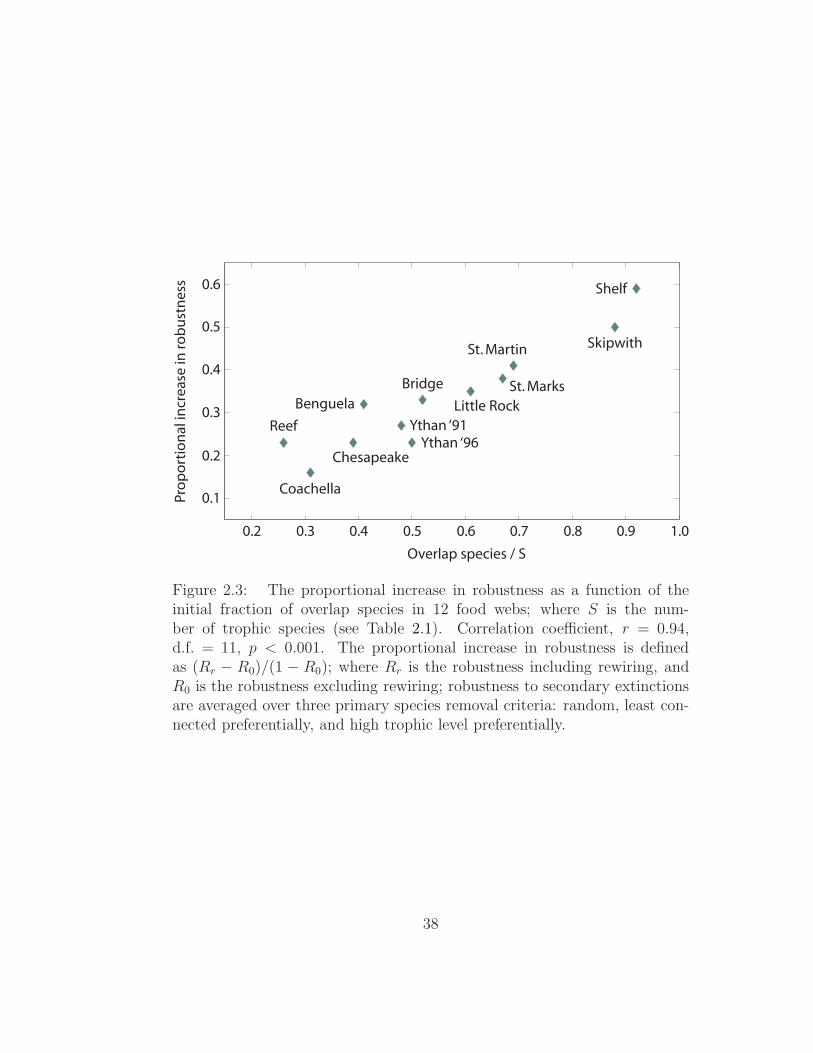
Figure 2.3: The proportional increase in robustness as a function of theinitial fraction of overlap species in 12 food webs; where S is the num-ber of trophic species (see Table 2.1). Correlation coefficient, r = 0.94,d.f. = 11, p < 0.001. The proportional increase in robustness is definedas (Rr − R0)/(1 − R0); where Rr is the robustness including rewiring, andR0 is the robustness excluding rewiring; robustness to secondary extinctionsare averaged over three primary species removal criteria: random, least con-nected preferentially, and high trophic level preferentially.
38

or connectance (r = 0.18, d.f. = 11, n.s.). However, we found a significant,
strong positive correlation between the proportional increase in robustness
and the initial fraction of overlap species in the food web (r = 0.94, d.f. = 11,
p < 0.001; Figure 2.3). We found that the initial fraction of overlap species is
approximately conserved in our removal simulations until there are very few
species remaining (data not shown). Thus, the fraction of overlap species in
general, not only the initial fraction, is a good indicator of the proportional
increase in robustness that can be expected in food webs when considering
structural dynamics compared to static topologies: the larger the fraction
of overlap species, the higher the proportional increase in robustness. This
positive correlation between the proportional increase in robustness and the
initial fraction of overlap species is observed even when each removal cri-
terion is considered individually: random, r = 0.91, d.f. = 11, p < 0.001;
least connected, r = 0.78, d.f. = 11, p = 0.003; high trophic level, r = 0.49,
d.f. = 11, n.s. Some highly-connected species, such as small pelagic fish and
invertebrates, are the particular target of human exploitation, and so results
for removing the most connected species preferentially are also of interest
(Dunne et al. 2004). Including this scenario in the criteria-averaged pro-
portional increase in robustness does not alter our results substantially: the
correlation with the initial fraction of overlap species is r = 0.90, d.f. = 11,
p < 0.001; and for the removal criterion individually, r = 0.79, d.f. = 11,
p = 0.002.
In Figure 2.2, the cumulative secondary extinction plots for the 12 food
webs are ordered by increasing initial fraction of overlap species, P . There
is no significant correlation between P and S (r = 0.13, d.f. = 11, n.s.), or
39

P and C (r = 0.04, d.f. = 11, n.s.). For example, the Coachella and Skipwith
food webs have very similar values for S and C (S = 29, 25; C = 0.31, 0.32; re-
spectively), but have very different values for P (P = 0.31, 0.88, respectively);
this leads to very different values for the proportional increase in robustness
(PIR = 0.16, 0.5, respectively), despite the food webs having similar ‘global’
structural characteristics. This suggests that the explicit topology of a food
web is important to determining its structural dynamics and robustness.
2.4 Discussion
Investigations of the structural robustness of empirical food webs increasingly
suggest that topological details greatly influence their simulated vulnerabil-
ity to secondary extinctions. Initial studies found that food webs are more
robust to random primary removal of species than to selective removal of
species with the most trophic links (Dunne et al. 2002). Food webs were
consistently more robust to our three ecologically plausible removal criteria
compared to removal of the most connected species preferentially (both or-
dered and probabilistic, data not shown), in agreement with a previous study
(Srinivasan et al. 2007). Attempts to find maximally destructive removal se-
quences suggest that the position of a species in the food web, rather than
its number of connections per se, is the main determinant of its impact on
extinction cascades (Allesina & Pascual 2009). Various structural indices
have been considered in attempts to identify functionally important species
in ecological networks (Jordan et al. 2008). One such measure, the trophic
overlap, uses the overlap of weighted trophic interaction data to quantify
the uniqueness of species’ interaction patterns (Jordan et al. 2009). How
40

these structural indices relate to properties of the overlap graph and overlap
species merits further investigation.
As acknowledged in earlier topological studies (Dunne et al. 2002), failure
to include a mechanism for predator-prey rewiring in simulations may result
in overestimates of the number of secondary extinctions following the removal
of individual species. We show that including rewiring in the topological ap-
proach consistently increases the robustness of food webs to primary species
removal. This finding is in many respects unsurprising: any model that re-
duces the loss of trophic links would be expected to increase the persistence
of the food web. However, how this additional robustness, generated by the
dynamic adaptation of trophic interactions, varies systematically with dif-
ferent properties of the food web is not obvious a priori. The proportional
increase in robustness was uncorrelated with the traditional food web met-
rics, species richness (S) and connectance (C), and was instead most highly
correlated with the initial fraction of overlap species (P ). This result was
robust to alternative definitions of trophic level and to non-random meth-
ods for selecting a new predator from the set of available potential predators
(data not shown). Within our predator-prey rewiring model, overlap species
are systematically defined: they are species in a food web’s rewiring graph
that have out-degree > 0 (see Figure 2.1). This definition means that overlap
species indicate the presence of potential predators in the food web. There
is no reason to suggest that overlap species should be such a good indica-
tor of the proportional increase in robustness when advancing from static to
dynamic food-web topologies. Knowledge of the initial fraction of overlap
species in a food web is insufficient for quantifying the precise number of
41

potential predators, nor the (maximum) number of trophic links that may
be retained due to rewiring; P also gives no indication of where those links
are located within the topological and trophic structure of the food web,
details especially pertinent given the cascading nature of secondary extinc-
tions. Furthermore, we find that another property derived from the overlap
graph—the connectance of the overlap graph—has no significant correlation
with the proportional increase in robustness (r = 0.34, d.f. = 11, n.s.; data
not shown). Thus, the fraction of overlap species appears to encapsulate, in
a very succinct way, the relevant structural features that ultimately influence
the proportional increase in robustness of empirical food webs.
So, how are we to understand overlap species? The introduction of struc-
tural dynamics to topological models of food web robustness highlights the
role of compensatory mechanisms in reducing secondary species extinctions
following environmental perturbations. Our identification of overlap species
represents an intriguing avenue for exploring how those compensatory mech-
anisms are related to the properties of individual species and the composite
roles they play within ecosystems. Understanding interaction patterns from
a biological perspective often requires a combination of phylogenetic infor-
mation and information on species’ ecological traits (Ives & Godfray 2006).
Increasingly detailed and comprehensive food-web data is becoming available
(Jacob 2005). These data make it feasible to compare species characteristics
(such as body-size, taxonomic identity, and geographical range) and commu-
nity and ecosystem characteristics (such as biomass and abundance) between
overlap and non-overlap species. Such additional information may also be
incorporated into decisions regarding the plausibility of trophic rewirings.
42

Phylogenetically related species tend to have similar biological characteris-
tics (Freckleton et al. 2002), and a phylogenetic approach has been used to
investigate constraints on trophic structure (Bersier & Kehrli 2008), patterns
of consumer-resource association (Ives & Godfray 2006), and coextinctions
in mutualistic networks (Rezende et al. 2007). A phylogenetic consideration
of overlap species would provide additional information on the relationship
between species’ characteristics and structural dynamics. Furthermore, ag-
gregation into trophic species is likely to underestimate the number of “real”
overlap species in a food web. These will be distributed non-randomly in
the food web, since trophic species contain more real species at lower trophic
levels (Williams & Martinez 2000). This will be an important consideration
for the identification of overlap species in the field.
In our predator-prey rewiring model, trophic adaptation (rewiring) re-
sults from changes in prey abundance brought about by species removal.
Three other factors can directly alter diet compositions and feeding rates:
changes in “habitat factors” such as temperature, water clarity, and soil
acidity; changes in predator feeding rates and search tactics; and changes
in predator abundance and competition. In our current model, if a trophic
rewiring is possible then it is established, but in reality competition among
predators for a prey species may prevent some rewirings from being realised.
This could be incorporated into the model by prescribing a probability for
the rewiring. Greater competition between predators would imply a smaller
probability of rewiring, and the overall effect would be a reduction in food-
web robustness relative to that observed in the current model.
Extinctions resulting from the loss of prey species represent the most pre-
43

dictable subset of secondary losses. Our structural approach may be consid-
ered a baseline that corresponds to the best-case scenario in which the min-
imum impact to the food web is taken into account. Although the predator-
prey rewiring model improves the evaluation of secondary extinctions, our
framework still underestimates the potential for cascading extinctions due
to strong non-trophic and indirect effects (Strauss 1991). In particular, the
robustness of food webs to preferentially removing species at high trophic
level may be altered significantly if the regulatory effects of top predators
are taken into account. Another important source of additional secondary
extinctions will be related to the bioenergetic or population dynamics of
species. Other forms of trophic adaptation have been shown to cause an in-
crease in food web persistence and stability. A population dynamic model on
static food-web topologies demonstrates that foraging adaptation may shift
the complexity-stability relationship of food webs from negative to positive
(Brose et al. 2003; Kondoh 2003, 2006; but see Garcia-Domingo & Saldana
2007). Despite much success on small, illustrative, food webs, the analysis
of removal effects using nonlinear differential equations remains challenging
for large ecological networks, requiring parameterisation of species interac-
tions with values that are often empirically unavailable (but see Borrvall &
Ebenman 2006; Brose et al. 2005). Nevertheless, there exists the prospect
of combining such bioenergetic and population dynamic models with a dy-
namic structure of trophic interactions. In a model of paleocommunity re-
sponse to species extinction, it was found that if consumers are permitted to
compensate for the loss of trophic resources by increasing the intensities of
their remaining biotic interactions, top-down secondary extinctions emerge
44

(Roopnarine 2006). Whether the effect of topological predator-prey rewiring,
which may mitigate the increase in intensity described above, would reduce
top-down secondary extinctions has not been considered. This is an exam-
ple where the combination of population and structural dynamics would be
necessary to assess fully the impact of species removal from a food web.
We have considered the implications of structural dynamics on the robust-
ness of empirical food webs. It would be instructive to apply the predator-
prey rewiring model to synthetic food webs generated by, for example, the
niche model. This would allow a comprehensive analysis of how structural
dynamics affect robustness as food web size and connectance is varied. Mod-
els that allow the contiguity of prey consumption to be varied (Williams &
Martinez 2008) provide a way of investigating the relationship between feed-
ing intervality and the ability of food webs to rewire. Such a study would also
be relevant to the analogous issue of nestedness and robustness in mutualistic
networks (Bascompte & Jordano 2007).
This study uses binary food webs that indicate the presence of a trophic
interaction but provide no information on the frequency of the interaction
or the rate of biomass flow through the interaction. The increasing avail-
ability of quantitative, weighted, trophic interaction data presents an op-
portunity for improving the realism of food-web robustness studies. Com-
pared to binary food webs, quantitative food webs more accurately describe
the structure and strength of trophic interactions and hence better inform
the sensitivity of species to environmental perturbations (Ings et al. 2009).
Future models should incorporate weighted information when determining
the rewiring of trophic interactions and when simulating the magnitude of
45

species loss.
In conclusion, our study underlines the importance of compensatory mech-
anisms that may buffer ecosystems against perturbations, and highlights par-
ticular species that are expected to facilitate those mechanisms. The consid-
eration of structural dynamics also enhances our understanding of the basic
robustness provided by food-web topologies. Differences in what could be
termed “structural plasticity” between empirical food webs, and the role of
overlap species in conferring structural robustness, has potential implications
for ecosystem conservation and management. Finally, the general method
for implementing structural dynamics that we have presented is amenable
to other approaches that seek to employ realistic food web structure and
dynamics.
Acknowledgements
We thank J. Dunne, C. Godfray, S. Saavedra, and three anonymous reviewers
for helpful comments on the manuscript.
References
Agrawal, A.A., Kobayashi, C. & Thaler, J. (1999). Influence of prey avail-
ability and induced host-plant resistance omnivory by western flower thrips.
Ecology, 80, 518–523.
Allesina, S. & Pascual, M. (2009). Googling food webs: can an eigenvec-
tor measure species’ importance for coextinctions? PLoS. Comp. Biol., 5,
e1000494.
46

Bascompte, J. & Jordano, P. (2007). Plant-animal mutualistic networks: the
architecture of biodiversity. Annu. Rev. Ecol. Evol. Syst., 38, 567–593.
Berlow, E.L., Dunne, J.A., Martinez, N.D., Stark, P.B., Williams, R.J. &
Brose, U. (2009). Simple prediction of interaction strengths in complex food
webs. Proc. Natl. Acad. Sci. USA, 106, 187–191.
Bersier, L.-F. & Kehrli, P. (2008). The signature of phylogenetic constraints
on food-web structure. Ecol. Complexity, 5, 132–139.
Borrvall, C. & Ebenman, B. (2006). Early onset of secondary extinctions in
ecological communities following the loss of top predators. Ecol. Lett., 9,
435–442.
Briand, F. & Cohen, J.E. (1984). Community food webs have scale-invariant
structure. Nature, 307, 264–266.
Brook, B.W., Sodhi, N.S. & Ng. P.K.L. (2003). Catastrophic extinctions
follow deforestation in Singapore. Nature, 424, 420–423.
Brose, U., Williams, R.J. & Martinez, N.D. (2003). Comment on ‘Foraging
adaptation and the relationship between food-web complexity and stability’.
Science, 301, 918a–918b.
Brose, U., Berlow, E.L. & Martinez, N.D. (2005). Scaling up keystone effects
from simple to complex ecological networks. Ecol. Lett., 8, 1317–1325.
Cohen, J.E. (1978). Food Webs and Niche Space. Princeton University Press,
Princeton, NJ.
47

Coll, M., Lotze, H.K. & Romanuk, T.N. (2008). Structural degradation in
Mediterranean sea food webs: testing ecological hypotheses using stochastic
and mass-balance modelling. Ecosystems, 11, 939–960.
Cousins, S.H. (1985). The trophic continuum in marine ecosystems: Struc-
ture and equations for a predictive model. Can. J. Fish. Aquat. Sci., 213,
76–93.
Dobson, A., Lodge, D., Alder, J., Cumming, G.S., Keymer, J., McGlade, J.,
et al. (2006). Habitat loss, trophic collapse, and the decline of ecosystem
services. Ecology, 87, 1915–1924.
Dunne, J.A., Williams, R.J. & Martinez, N.D. (2002). Network structure
and biodiversity loss in food webs: robustness increases with connectance.
Ecol. Lett., 5, 558–567.
Dunne, J.A., Williams, R.J. & Martinez, N.D. (2004). Network structure
and robustness of marine food webs. Mar. Ecol. Prog. Ser., 273, 291–302.
Dunne, J.A. & Williams, R.J. (2009). Cascading extinctions and community
collapse in model food webs. Phil. Trans. R. Soc. B, 364, 1711–1723.
Ebenman, B., Law, R. & Borvall, C. (2004). Community viability analysis:
the response of ecological communities to species loss. Ecology, 85, 2591–
2600.
Fath, B.D., Scharler, U.M., Ulanowicz, R.E. & Hannon, B. (2007). Ecological
network analysis: network construction. Ecol. Model., 208, 49–55.
48

Freckleton, R., Harvey, P. & Pagel, M. (2002). Phylogenetic analysis and
comparative data: a test and review of evidence. Am. Nat., 160, 712–26.
Garcia-Domingo, J.L. & Saldana, J. (2007). Food-web complexity emerging
from ecological dynamics on adaptive networks. J. Theor. Biol., 247, 819–
826.
Gentleman, W., Leising, A., Frost, B., Strom, S. & Murray, J. (2003). Func-
tional responses for zooplankton feeding on multiple resources: a review of
assumptions and biological dynamics. Deep Sea Res. II, 50, 2847–2875.
Hutchinson, G.E. (1957). Concluding remarks. Cold Spring Harb. Symp.
Quant. Biol., 22, 415–427.
Ings, T.C., Montoya, J.M., Bascompte, J., Bluthgen, N., Brown, L., Dor-
mann, C.F., et al. (2009). Ecological networks—beyond food webs. J.
Anim. Ecol., 78, 253–269.
Ives, A.R. & Godfray, H.C.J. (2006). Phylogenetic analysis of trophic asso-
ciations. Am. Nat., 168, E1–E14.
Jacob, U. (2005). Trophic Dynamics of Antarctic Shelf Ecosystems—Food
Webs and Energy Flow Budgets. University of Bremen, Germany, Thesis,
125 pp.
Jordan, F., Okey, T.A., Bauer, B. & Libralato, S. (2008). Identifying im-
portant species: linking structure and function in ecological networks. Ecol.
Model., 216, 75–80.
49

Jordan, F., Liu, W.-C. & Mike, A. (2009). Trophic field overlap: a new
approach to quantifying keystone species. Ecol. Model., 220, 2899–2907.
Kondoh, M. (2003). Foraging adaptation and the relationship between food-
web complexity and stability. Science, 299, 1388–1391.
Kondoh, M. (2006). Does foraging adaptation create the positive complexity-
stability relationship in realistic food-web structure? J. Theor. Biol., 238,
646–651.
Levine, S. (1980). Several measures of trophic structure applicable to com-
plex food webs. J. Theor. Biol., 83, 195–207.
Martinez, N.D. (1991). Artifacts or attributes? Effects of resolution on the
Little Rock Lake food web. Ecol. Monogr., 61, 367–392.
Martinez, N.D., Hawkins, B.A., Dawah, H.A. & Feifarek, B.P. (1999). Effects
of sampling effort on characterization of food-web structure. Ecology, 80,
1044–1055.
Pascual, M. & Dunne, J.A. (2006). Ecological Networks: Linking Structure
to Dynamics in Food Webs. Oxford University Press, USA.
Pastorok, R.A. (1980). The effects of predator hunger and food abundance
on prey selection by Chaoborus larvae. Limnol. Oceanogr., 25, 910–921.
Petchey, O.L., Beckerman, A.P., Riede, J.O. & Warren, P.H. (2008). Size,
foraging and food web structure. Proc. Natl. Acad. Sci. USA, 105, 4191–
4196.
50

Pimm, S.L. (1991). The Balance of Nature. The University of Chicago Press,
Chicago, IL, pp. 240–241.
Raffaelli, D. (2004). How extinction patterns affect ecosystems. Science,
306, 1141–1142.
Rezende. E.L., Lavabre, J.E., Guimaraes, P.R, Jordano, P. & Bascompte, J.
(2007). Non-random coextinctions in phylogenetically structured mutualistic
networks. Nature, 448, 925–929.
Roopnarine, P.D. (2006). Extinction cascades and catastrophe in ancient
food webs. Paleobiology, 32, 1–19.
Roopnarine, P.D., Angielczyk, K.D., Wang, S.C. & Hertog, R. (2007). Trophic
network models explain instability of Early Triassic terrestrial communities.
Proc. R. Soc. B, 271, 2077-2086.
Saavedra, S., Reed-Tsochas, F. & Uzzi, B. (2008). Asymmetric disassembly
and robustness in declining networks. Proc. Natl. Acad. Sci. USA, 105,
16 466–16 471.
Shin, Y.-J., Shannon, L.J. & Cury, P.M. (2004). Simulations of fishing effects
on the southern Benguela fish community using an individual-based model:
learning from a comparison with ECOSIM. Afr. J. Mar. Sci., 26, 95–114.
Srinivasan, U.T., Dunne, J.A., Harte, J., & Martinez, N.D. (2007). Response
of complex food webs to realistic extinction sequences. Ecology, 88, 671–682.
Strauss, S.Y. (1991). Indirect effects in community ecology: their definition,
51

study and importance. Trends Ecol. Evol., 6, 206–210.
Thompson, R.M. & Townsend, C.R. (2005). Energy availability, spatial het-
erogeneity and ecosystem size predict food-web structure in streams. Oikos,
108, 137–148.
Williams, R.J. & Martinez, N.D. (2000). Simple rules yield complex food
webs. Nature, 404, 180–183.
Williams, R.J. & Martinez, N.D. (2004). Limits to trophic levels and om-
nivory in complex food webs: theory and data. Am. Nat., 163, 458–468.
Williams, R.J. & Martinez, N.D. (2008). Success and its limits among struc-
tural models of complex food webs. J. Anim. Ecol., 77, 512–519.
Woodward, G., Ebenman, B., Emmerson, M., Montoya, J.M., Olesen, J.M.,
Valido, A., et al. (2005). Body size in ecological networks. Trends Ecol.
Evol., 20, 402–409.
52

Chapter 3
Active reallocation of food-web
interactions under
environmental change
Human-induced habitat modification is the primary driver of worldwide changes
in the diversity and composition of species (Millennium Ecosystem Assess-
ment 2005). However, it is less clear how environmental change affects the
patterns of interactions among species (Tylianakis et al. 2008). Although
the structure of ecological communities (Memmott et al. 1994; Muller et al.
1999) is known to vary across gradients of habitat modification (Tscharntke et
al. 1998; Klein et al. 2006; Tylianakis et al. 2007; Albrecht et al. 2007), the
processes responsible for these changes are unknown. Here we show that vari-
ability in consumer functional response among habitats lead to interaction
distributions that cannot be explained purely on the basis of resource avail-
ability. We apply a simple model of consumer feeding to data on insect hosts
and their natural enemies from four regions. The model accurately recreates
observed changes in quantitative food-web structure following habitat mod-
ification. The model highlights two processes responsible for changes to the
53

distribution of interactions: altered selection within a consumer’s existing re-
source set, and the initiation of novel trophic interactions. In environments
where communities are more impacted by habitat modification, interaction
patterns increasingly depart from density-dependent resource selection. Our
findings are consistent with improved consumer foraging efficiency in simpli-
fied environments, where increased resource selectivity can lead to greater
than expected specialisation, while increased resource encounters can also
lead to greater than expected generalisation. Understanding how variation
in trophic specialisation is generated will improve forecasts of the community-
level impact of environmental change and its implications for ecosystem func-
tioning.
3.1 Introduction
A central goal in ecology is to explain and predict the structure of species
interaction networks (Memmott 1999; Lewis et al. 2002; Montoya et al.
2006). Environmental change can lead to the disappearance of species from
ecosystems and cause alterations to the abundance of those species that per-
sist (Foley et al. 2005). Consequently, understanding how anthropogenic
changes affect the dynamics and function of ecological networks is an im-
portant theoretical challenge, but is also likely to have significant practical
consequences since humans rely on the ecosystem services associated with
species interactions such as pollination, seed dispersal, and biological con-
trol (Costanza et al. 1997; Losey & Vaughan 2006). Theoretical studies
exploring changes in community composition have typically assumed that
food-web topology remains unchanged even as species are removed, although
54

recent work has proposed mechanisms that allow for structural adaptation
(Kondoh 2003; Kaiser-Bunbury et al. 2010; Staniczenko et al. 2010). Ad-
vances in field methods that quantify functionally-important variations in the
magnitude or frequency of interactions (Muller et al. 1999) have generated
highly-detailed food webs that not only provide a more robust description of
static community structure (Banasek-Richter et al. 2004), but also enable
more accurate insights into dynamic and indirect interactions among species
(Morris et al. 2004; Laliberte & Tylianakis 2010). This increasing availabil-
ity of rich, community-level, data requires a parallel advance in theoretical
models to explain the mechanisms underpinning quantitative, rather than
binary (interaction presence-absence), food webs.
Diets of species are largely constrained by their phylogenetic history and
morphology (Ives & Godfray 2006). However, the composition of a con-
sumer’s diet can alter depending on resource availability and quality in dif-
ferent environments (Stang et al. 2009). A useful initial null hypothesis
that avoids assuming specific behavioural processes is that interactions are
primarily determined by resource species density (Vazquez et al. 2007). In
the simplest case, we assume a linear response between consumer interac-
tion frequency and resource density, with the explicit form of the relation-
ship remaining independent of environment. We call this constant functional
response density-dependent reallocation (i.e., interactions are allocated pas-
sively in modified environments, entirely according to changes in resource
density). However, consumer functional response is unlikely to remain con-
stant in modified habitats, due to effects such as different preferences for
resource species and altered foraging efficiency (Pulliam 1974). We call such
55

flexible functional response active reallocation.
Our simple model of active reallocation quantifies and characterises this
dynamic process, and provides significantly better agreement with empiri-
cal data compared to density-dependent reallocation. It clarifies the role
of novel trophic interactions—also known as switches (Murdoch 1969)—and
provides a base model that can help identify more specific ecological mech-
anisms that lead to altered trophic-breadth in different environments. The
model allows consumer selectivity to increase or decrease, so that the cor-
responding distribution of interactions becomes, respectively, more specific
(over-specialisation) or more general (over-generalisation) than would be ex-
pected from density-dependent reallocation.
3.2 Materials and Methods
The information contained in food webs can be summarised in various ways.
Quantitative, weighted, equivalents of binary food-web statistics have been
developed (Bersier et al. 2002) and used extensively. The weighted con-
nectance (Cq) quantifies the amount of potential interactions that are re-
alised in the food web; the interaction diversity (Iq) quantifies the evenness
of the interactions between species; the generality (Gq) quantifies the average
number of resource species weighted by consumer abundance; and the vul-
nerability (Vq) quantifies the average number of consumer species weighted
by resource abundance (see Appendix 3.5.1). This set of metrics provide
consumer-centric, resource-centric and complete food-web summaries of in-
teractions and we used them to assess the structure of food webs across
different gradients of habitat modification in Germany, Ecuador, Indonesia
56

and Switzerland.
These food webs focus on a subset of interactions involving insects at
two trophic levels: parasitoid species (consumers) and their host species
(resources). Similar methods were used to collect food-web data from the
different regions presented here, facilitating comparison. Pooling of replicate
webs within regions was necessary to maximise resolution on the webs and
minimise the possibility of artefacts due to low sampling effort (Tylianakis
et al. 2010). Patterns of parasitoid-host interactions have been shown previ-
ously to differ between forested and unforested habitats (including no to few
individual trees), and more complex compared to more simple environments
(Tylianakis et al. 2007; Laliberte & Tylianakis 2010). Therefore, we assem-
bled quantitative bipartite webs representative of less-open (hereafter com-
plex) and more-open (hereafter simple) environments in each region (Table
3.1, Figure 3.1). These categorisations were based on replicate web metadata
such as ground-level light intensity and plant species richness. There are clear
differences in the distribution of interaction frequencies among environments
and among regions (Table 3.2).
We used the difference in the Shannon evenness index (Krebs 1989) of
host species between webs (∆, Table 3.1) as a measure of the community
impact generated by habitat modification. The Shannon evenness for each
region was normalised by the maximum value it could take to get a measure
in the range [0,1]:
E =−
∑Ni=1 pilog2pi
log2N, (3.1)
where the numerator is the Shannon entropy for N host species, pi is the
57

Region Hosts Paras Complex food web Simple food web ∆ R S Switches
Indonesiaa 11 25 Agroforest, 12 highly Agroforest, 12 less -0.078 1.225 0.05 26 (53)forested replicates forested replicates
Germanyb 26 9 Orchard meadow Field margin strip -0.087 1 1.6 13 (55)Ecuadorc 19 8 Forest, managed and Pasture, rice 0.145 0.975 1.3 16 (45)
abandoned coffee agroforestSwitzerlandd 20 16 Restored meadow Intensively-managed 0.169 2.775 0.15 17 (59)
ecological compensation meadow 25m, 50m andarea (ECA) 100m from ECA
Table 3.1: Food-web descriptions and active reallocation model parameters. Complex and simple food webs areobtained by pooling replicate webs from representative environments in each region. Regions are ordered by thedifference in Shannon evenness index of hosts between webs (∆): larger values suggest increased within-regioncommunity impact due to modification; negative values imply increasing homogenisation in the distribution of hostspecies, with positive values implying increasing heterogeneity. R and S are community-level parameters used inthe active reallocation model. Switches are given relative to the total number of host-parasitoid interactions.
aKlein et al. 2006bStudy 3 in Tscharntke et al. 1998cTylianakis et al. 2007dAlbrecht et al. 2007
58

Region Complex web Simple web Model Null 1 Null 2
Weighted ConnectanceEcuador 0.179 0.068 0.068 0.062 0.056Germany 0.093 0.119 0.119 0.124 0.091Indonesia 0.103 0.131 0.119 0.112 0.099Switzerland 0.100 0.078 0.077 0.086 0.095
Interaction DiversityEcuador 3.82 1.79 1.77 1.42 1.13Germany 4.13 4.01 3.95 4.41 3.92
Indonesia 3.84 4.46 4.33 4.18 3.46Switzerland 4.52 4.03 3.91 4.09 3.84
GeneralityEcuador 8.04 2.10 2.11 2.07 1.99Germany 4.06 6.34 6.35 6.32 4.16Indonesia 1.92 2.69 2.44 2.73 1.64Switzerland 4.64 2.58 2.66 3.46 3.32
VulnerabilityEcuador 1.59 1.55 1.56 1.26 1.06Germany 2.09 1.51 1.53 1.87 1.83Indonesia 5.52 6.76 6.12 5.32 5.48Switzerland 2.58 3.00 2.91 2.73 2.39
Table 3.2: Empirical metric values and model results. See Table 3.1 for adescription of food webs and active reallocation model parameters. Null 1corresponds to the density-dependent reallocation model; Null 2 is as Null1 but does not include switches. Entries in bolded-italics indicate valueswithin 5% of the empirical, simple environment, metric.
59

1 2 3 4 5 6 7 8 9 10 11 12 13 14 15 16
A B C D E F G H I J K L M N O P Q R S T
1 2 3 4 5 6 7 8 9 10 1112 13 14 15 16
A B C D E F G H I J K L M N O P Q R S T
Figure 3.1: Quantitative parasitoid-host food webs in complex (left) andsimple environments (right) for the Switzerland data. For each web, lowerbars represent host (bee and wasp) density and upper bars represent par-asitoid density, drawn at different scales. Linkage width indicates the fre-quency of each trophic interaction. Interactions are classified as switches(novel interactions) if they appear in the simple but not complex environ-ment (highlighted in green).
proportional density for host species i, and the denominator is the maximum
possible evenness of the distribution. We compare the environments of com-
plex and simple webs using ∆ = Ecomplex −Esimple. ∆ close to zero indicates
little change in host distribution, implying little impact due to modification
between complex and simple environments; larger values suggest increased
impact. Negative values imply increasing homogenisation in the distribution
of host species, with positive values implying increasing heterogeneity. This
analysis leads to the following ordering from least-to-most severely altered
region: Indonesia, Germany, Ecuador, and Switzerland (Table 3.1).
We model quantitative food-web structure in simple environments using
data from complex environments. We begin by assuming that each interac-
tion between host i and parasitoid j in the complex food web follows a linear
functional response
yij = mijxi , (3.2)
60

where mij is the observed per-capita attack rate (i.e., the empirical number
of parasitism events divided by the host density). To assess whether the
assumption of linear functional response is reasonable, we fit Type I (lin-
ear) and Type II (saturating) functional forms to complex web interactions
where more than three replicate web interactions contribute to a pooled web
interaction. For the Type II functional response, we performed a non-linear
least-squares fit with a Michaelis-Menten form
yij =vijxi
Kij + xi
, (3.3)
where vij is the saturation interaction strength, and Kij is the rate constant.
We assigned a classification—linear or saturating—as the form giving the
lowest mean square error following the least-squares procedure (assuming the
saturating form has biologically-reasonable parameters, i.e., the rate constant
should not be negative). In our complex web data, we found that the majority
(72%) of interactions permitting classification were better fit by a linear
rather than saturating functional form. A Type III (sigmoidal) response
was not considered here because the limited number of data points for each
pooled web interaction would make distinguishing between Type II and Type
III forms very difficult. The majority of interactions (73% across Indonesia,
Ecuador and Switzerland) in each pooled web were observed in only one of
the contributing replicate webs. For these interactions, we can only assume
the most parsimonious possibility of a linear response between interaction
frequency and resource density. Germany did not have a sufficient number
of replicate webs for this analysis.
With density-dependent reallocation, by definition, the set of m-coefficients
61

is independent of the environment. Consequently, we can use Equation 3.2
(parameterised from the complex environment) to model the interaction dis-
tribution for each parasitoid species in a simple environment (e.g., after habi-
tat modification), given a new empirical distribution of host species. We
compare this density-dependent deterministic model to empirical data from
the simple environment by running stochastic simulations of parasitoid-host
interactions that incorporate two sources of uncertainty: i) error arising from
differences in observed per-capita attack rates among replicate webs; and ii)
error arising from requiring integer numbers for interaction events.
We quantified variation in the per-capita attack rate (the number of par-
asitism events divided by the host density, mij in Equation 3.2) between
replicate webs using linear least-squares regression. Where more than three
replicate web interactions contributed to a pooled interaction, we recorded
the standard deviation of the residuals and the pooled number of para-
sitism events (pooled interaction frequency). Since we are conducting a
least-squares minimisation, residuals are approximately normally distributed
(mean zero) with their standard deviation representing the error on the true
value of a pooled interaction. Compiling all interactions, we fit a linear rela-
tionship between pooled interaction frequency, J , and the expected error in
that value: σJ = a+bJ , where a and b are constants from a linear regression.
We used this relationship to incorporate per-capita attack-rate uncertainty
into simulations of species interactions in simplified environments. For a
given deterministic prediction for the frequency of an interaction, the er-
ror on that value is drawn from a normal distribution with mean zero and
standard deviation σJ .
62

Simulations provided an expected frequency-weighted interaction gener-
ality for each parasitoid species, with an associated standard deviation, which
was compared to empirical data using the z-score. The diversity of interac-
tion inflows to a consumer k is,
Hk = −r
∑
i=1
bik
b•klog2
bik
b•k, (3.4)
where bik is the interaction contribution from resource i and b•k is the total
interaction frequency into k, for a total of r resource species. The number of
resource species a consumer has (weighted according to their use frequency) is
then nk = 2Hk . The empirical value for nk can be compared to the interaction
distribution generated by density-dependent reallocation (Null model 1, see
below) using the z-score
zk =〈nk〉 − n∗
k
σnk
, (3.5)
where n∗
k is the empirical value, 〈nk〉 is the average value of an ensemble of
model randomisations and σnkis the standard deviation of the same quan-
tity. Values of zk > 0 indicate over-specialisation and zk < 0 indicate over-
generalisation.
The active reallocation model is deterministic and, as with density-dependent
reallocation, begins by assuming that interactions follow a linear functional
response (see Appendix 3.5.2). However, the set of m-coefficients for a para-
sitoid species can be altered between environments by two community-level
parameters, R (resource-based changes) and S (switch-specific changes). The
parameters take positive values and adjust the dispersion of m-coefficients for
each parasitoid species: R, S > 1 “stretches” consumer interaction distribu-
tions (m-coefficients become more different), thereby promoting preference
63

of some hosts over others; whereas R, S < 1 “compresses” consumer interac-
tion distributions (m-coefficients become more similar), thereby homogenis-
ing host preference. The model permits two additional modes of consumer
behaviour compared to density-dependent reallocation: i) consumer inter-
action frequencies can change in a non-linear way following changes in re-
source density (through R); and ii) switches—interactions that are absent
in the complex web but present in the simple web—are afforded a separate
role to existing interactions in determining quantitative food-web structure
(through S). We set parameter values giving closest agreement with the em-
pirical data (deterministic model, Table 3.1) and run stochastic simulations
as with density-dependent reallocation.
We compare the reallocation model to two null models. Null model 1
corresponds to density-dependent reallocation and assumes that changes in
interaction frequency (including switches) are solely determined by changes
in resource density. Null model 2 is as Null model 1 but does not include
switches; it assumes that the maximum possible set of interactions in the
simple food web remains the same as in the complex food web.
The closeness of a model quantitative food-web metric, Q∗, to the empir-
ical value, Q, is
δQ =
∣
∣
∣
∣
∣
Q∗ − Q
Q
∣
∣
∣
∣
∣
, (3.6)
values closer to 0 indicate better agreement with the empirical value. Close-
ness to empirical data is measured by assessing all four metrics jointly for
each simulation run, and we use the largest value of δQ as our measure.
However, we find similar qualitative results if the average of the individual
64

metric closeness values is used rather than taking the maximum value for the
closeness.
3.3 Results
In simple environments, empirical data displayed significant deviation from
density-dependent reallocation with a clear community trend (Figure 3.2).
In Indonesia we primarily observed over-generalisation of parasitoid inter-
actions, while in Germany, Ecuador and Switzerland we primarily observed
over-specialisation. Generalist parasitoid species (those with a broad host
range) tended to display greater over-specialisation (Pearson correlation be-
tween positive z-score and weighted interaction generality: r = 0.51, d.f.
= 18, p = 0.02; Figure 3.3). Thus, in simplified environments, more gen-
eralist parasitoids (as measured in the complex environments) tended to
over-specialise to a greater degree than less-generalist parasitoids. However,
there was no significant relationship between the absolute z-score for over-
generalisation (interactions with a negative z-score) and parasitoid interac-
tion generality (Pearson correlation: r = −0.21, d.f. = 17, p = 0.39).
Of 58 parasitoid species across the 4 regions, 19 were specialists with
interactions to only one host, and were excluded from this analysis. We
observed over-specialisation (positive z-score) in 20 parasitoid species (8 with
a z-score > 1.96, individual test significance p < 0.05) and over-generalisation
(negative z-score) in 19 parasitoid species (4 with a z-score < -1.96, p < 0.05,
all in the Indonesia data set).
Following Moran (2003), we can assess how likely it would be to obtain
the observed number of statistically significant—individual test—incidences
65

Indonesia Germany Ecuador Switzerland−8
−6
−4
−2
0
2
4
6
8
10
z−sc
ore
Figure 3.2: Empirical parasitoid generality in simple environments com-pared to a density-dependent reallocation model for four regions. Density-dependent reallocation assumes constant, linear, parasitism functional re-sponse between complex and simple environments. Each point representsa parasitoid species, with 10,000 simulations per parasitoid for each region.A z-score > 0 indicates over-specialisation, a z-score < 0 indicates over-generalisation; values exceeding ±1.96 have significance p < 0.05 (horizontaldashed lines). Parasitoids with only one interaction have a z-score = 0 byconstruction and are omitted.
66

1 2 3 4 5 6 7 8 90
1
2
3
4
5
6
7
8
9
Parasitoid interaction generality
z−sc
ore
Figure 3.3: The z-score for over-specialisation is positively correlated withfrequency-weighted parasitoid interaction generality. (Pearson correlation,r = 0.51, d.f. = 18, p = 0.02). If the data point with a very high z-score (≈ 9) is removed, then the Pearson correlation is r = 0.42, d.f. = 17,p = 0.07.
67

of over-specialisation and over-generalisation within regions by chance. The
probability of X individual tests being statistically significant (at the p <
0.05 level) out of Y tests can be calculated using a Bernoulli process (see
Moran 2003 for details). In Indonesia we observed 4 significant individual
tests out of 11, giving a probability of 0.001 that this result would occur
by chance; in Germany the probability is 0.0054 (3 out of 8 significant); in
Ecuador the probability is 0.28 (1 out of 8 significant); and in Switzerland
the probability is 0.002 (4 out of 12 significant).
A more conservative assessment of the significance of our results can be
obtained by applying sequential Bonferroni (single-tailed significance, see
Moran 2003 for a description). Sequential Bonferroni increases the level at
which an individual test can be considered significant based on the number
of tests performed. It provides a complementary assessment to the Bernoulli
method, which does not alter the significance level between individual and
multiple hypothesis testing. Using sequential Bonferroni, we strongly reject
the null hypothesis (meaning that the z-scores can be considered significant)
for two parasitoids in Indonesia, two parasitoids in Germany, one parasitoid
in Ecuador, and one parasitoid in Switzerland. Thus, density-dependent
reallocation was insufficient to fully explain empirical data.
The active reallocation model is deterministic and has two community-
level parameters: R (resource-based changes) and S (switch-specific changes).
We set parameter values giving closest agreement to the empirical data. In
the parameter spaces of Ecuador, Germany and Indonesia (Figures 3.4–3.6),
the values of R and S that provide the best agreement with the empirical
data (lowest closeness values) are restricted to relatively small ranges. How-
68

S
R
0 0.25 0.5 0.75 1 1.25 1.5 1.75 2
0
0.5
1
1.5
2
2.5
3
3.5
4
4.5
5 0
0.2
0.4
0.6
0.8
1
Figure 3.4: Active reallocation model parameter space for Ecuador. Close-ness (scale on right-hand-side) to empirical data is measured by assessing allfour food-web metrics jointly; values closer to 0 indicate better agreementwith empirical data. Best-fit parameter values R = 0.975, S = 1.3.
ever, in the Switzerland parameter space (Figure 3.7), the closeness remains
essentially the same for the range of S-values considered. This indicates that
S does not significantly contribute to altering the distribution of consumer-
resource interactions in the simple environment. The best-fit value, S =
0.15, was used in stochastic simulations, but results are similar if values of
0 < S < 2 are used.
The active reallocation model provided good agreement with empirical
data, and significantly out-performed two null models (Figure 3.8 and Ta-
ble 3.2): i) density-dependent reallocation (Null model 1); and ii) density-
dependent reallocation excluding switches (Null model 2). The success of the
model emphasises that consumer selectivity can change substantially follow-
ing habitat modification. With regions ordered by changes in the Shannon
69

S
R
0 0.25 0.5 0.75 1 1.25 1.5 1.75 2
0
0.5
1
1.5
2
2.5
3
3.5
4
4.5
5 0
0.2
0.4
0.6
0.8
1
Figure 3.5: Active reallocation model parameter space for Germany. Close-ness (scale on right-hand-side) to empirical data is measured by assessing allfour food-web metrics jointly; values closer to 0 indicate better agreementwith empirical data. Best-fit parameter values R = 1, S = 1.6.
S
R
0 0.25 0.5 0.75 1 1.25 1.5 1.75 2
0
0.5
1
1.5
2
2.5
3
3.5
4
4.5
5 0
0.2
0.4
0.6
0.8
1
Figure 3.6: Active reallocation model parameter space for Indonesia. Close-ness (scale on right-hand-side) to empirical data is measured by assessing allfour food-web metrics jointly; values closer to 0 indicate better agreementwith empirical data. Best-fit parameter values R = 1.225, S = 0.05.
70

S
R
0 0.25 0.5 0.75 1 1.25 1.5 1.75 2
0
0.5
1
1.5
2
2.5
3
3.5
4
4.5
5 0
0.2
0.4
0.6
0.8
1
Figure 3.7: Active reallocation model parameter space for Switzerland.Closeness (scale on right-hand-side) to empirical data is measured by assess-ing all four food-web metrics jointly; values closer to 0 indicate better agree-ment with empirical data. Best-fit parameter values R = 2.775, S = 0.15.
evenness of hosts, we find that as communities become more impacted, the
relative performance of the active reallocation model compared to Null model
1 increases (Figure 3.8). This result is consistent with increasingly simplified
environments permitting more efficient foraging (Gols et al. 2005; Laliberte
& Tylianakis 2010), such that parasitoids can be more selective in the hosts
they parasitise.
3.4 Discussion
We further assess the effect of habitat modification on resource selection by
considering the parameter values obtained for each region (Table 3.1). In
Switzerland, habitat simplification and homogenisation may have enabled
particular—presumably preferred—hosts to be located more easily by par-
71

Indonesia Germany Ecuador Switzerland0
0.1
0.2
0.3
0.4
0.5
Clo
sene
ss
Figure 3.8: Increasing impact of within-region habitat modification (left-to-right) leads to greater separation between the active reallocation (circles,mean ± s.d.) and density-dependent reallocation (squares) models. Density-dependent reallocation excluding switches (triangles) performs significantlyworse in all regions. Closeness is defined as the percentage difference be-tween model and data for the worst-performing food-web metric of the set{Cq, Iq, Gq, Vq} and lower values indicate better agreement with empiricaldata. The same trend is observed if the average of the individual metriccloseness values is used rather than taking the maximum value for the close-ness. Data are shown for 10,000 simulations per model for each region.Regions are ordered by the impact of habitat modification, which is given bychanges in the Shannon evenness index of hosts (∆, values in Table 3.1).
72

asitoids, driving over-specialisation within existing interactions (R > 1; S
not significant, see Figure 3.7). In Ecuador and Germany, switches drove
over-specialisation and some of those interactions were to preferred hosts
(R ∼ 1; S > 1); in Indonesia, switches drove over-generalisation but those
interactions were treated homogenously (R ∼ 1; S ∼ 0). We suggest the fol-
lowing explanation for this difference. The habitat modification in Germany,
Ecuador and Switzerland can, independent of changes in host diversity, be
considered more severe than in Indonesia (where all replicate webs are from
the same agroforest compared to different habitat classes in the other three
regions). In less-severe simple habitats, parasitoids can locate a broader
range of preferred hosts compared to a reduced set of host species in more-
severe habitats. In Indonesia, over-generalisation is expected if conversion
into more simple environments primarily increases the chance of parasitoids
coming into contact with hosts. This interpretation is also consistent with
differences in the functional response of switches between regions.
We assumed a linear functional form for the relationship between inter-
action frequency (parasitism) and host density. The success of the active
reallocation model compared to the density-dependent reallocation model
indicates that parasitoid preference for hosts can change substantially fol-
lowing habitat modification. We suggested that this result is consistent with
increasingly simplified environments permitting more efficient foraging (Gols
et al. 2005; Laliberte & Tylianakis 2010), such that parasitoids can be more
selective in the hosts they parasitise. This behaviour is consistent with re-
sults observed for the parasitoid species Ichneumonidae sp.3 in Indonesia, and
Melittobia acasta in both Ecuador and Switzerland. Melittobia is a very gen-
73

eralist parasitoid species, which affords it greater flexibility in selecting from
available hosts compared to more inherently specialist parasitoid species.
The model showed that switches could play significantly different roles
between regions and that neglecting switches all together (Null model 2)
produced very poor agreement with empirical data (see Figure 3.8). We
examined switches more closely by comparing the set of functional responses
suggested by the simple environment data to those suggested by the complex
environment data. We observed different functional responses for switches
in Ecuador and Switzerland compared with Indonesia (as before, Germany
does not have a sufficient number of replicate webs for this analysis).
In Ecuador and Switzerland, the data suggest that switches are consis-
tent with the low- to mid-density regime of a Type III (sigmoidal) functional
response; that is, there is essentially no parasitism at low host densities, fol-
lowed by increasing rates of parasitism as host density increases. This con-
firms a very natural expectation of how the functional response of switches
should differ from existing interactions. Thus, the linear approximation—
drawn from data comprising complex environments only—underestimates
the magnitude of the functional response. This lends credence to increas-
ing the relative importance of switches compared to existing interactions in
the active reallocation model (we add 1 to the relative density change for
switches to ensure that they are always positive, see Appendix 3.5.2). In
Ecuador, switches are observed to drive over-specialisation in the parasitoid
species Coelioxys sp. and Chrysis sp.; switches are treated no differently from
existing interactions in Switzerland.
In Indonesia, the functional response of switches in the simple environ-
74

ment is again consistent with the low-density to mid-density regime of a
Type III functional response. However, if host densities from the complex
environment are included when assessing the functional response, a negative
response is suggested (increasing host density leads to fewer interactions).
This is because no host-parasitoid interactions (of the subset of switches)
were observed in the complex environments despite greater host density com-
pared with the simple environments. In the less-severe habitat of Indonesia,
simplified environments primarily increase the chance of parasitoids com-
ing into contact with hosts—parasitoids can thus locate a greater variety of
(preferred) hosts. In this case, the more efficient foraging permitted by sim-
plified habitats can lead to switches driving over-generalisation, as observed
in the parasitoid species Chrysis smaragdula, Stilbum chrysocephalum, and
Tachinidae sp.1 and sp.2.
Pure density-dependent resource selection, whilst providing an informa-
tive qualitative assessment, cannot account for all changes in quantitative
food-web structure following habitat modification. Changes in consumer
behaviour (illustrated by changes in functional response) between habitats
must also be considered. In simplified environments, novel trophic interac-
tions were formed and feeding preferences were observed to adjust to new
host assemblages. The active reallocation model does not specify underlying
behavioural mechanisms beyond altered consumer preference and provides
substantial motivation for incorporating species’ behaviour into food web re-
search. Indeed, our results are consistent with increased parasitoid foraging
efficiency in simplified environments. The model accurately generates quan-
titative interaction frequencies in non-size-structured food webs (i.e., where
75

resource use is not limited by consumer body size) and represents a significant
advance towards the important goal of modelling realistic consumer feeding
(Ings et al. 2009). Food-web structure is dynamic and influenced both by
environmental factors, such as resource distribution and availability, and by
species-level factors such as behaviour and resource preference. Understand-
ing the mechanisms underlying altered trophic-breadth and selective species
interactions will help with the planning of habitat restoration projects and in
assessing their efficacy. Adaptive functional response—active reallocation—
needs to be taken into account when developing forecasts of the effects of
human-induced disturbances on community structure and composition.
Acknowledgements
We thank S. Allesina, C. Godfray and S. Saavedra for comments on an earlier
version of the manuscript.
References
Albrecht, M., Duelli, P., Schmid, B. & Muller, C.B. (2007). Interaction diver-
sity within quantified insect food webs in restored and adjacent intensively
managed meadows. J. Anim. Ecol., 76, 1015–1025).
Banasek-Richter, C., Cattin, M.F. & Bersier, L.F. (2004). Sampling effects
and the robustness of quantitative and qualitative food-web descriptors. J.
Theor. Biol., 226, 23–32.
Bersier, L.F., Banasek-Richter, C. & Cattin, M.F. (2002). Quantitative de-
scriptors of food-web matrices. Ecology, 83, 2394–2407.
76
Costanza, R. et al. (1997). The value of the world’s ecosystem services and
natural capital. Nature, 387, 253–260.
Foley, J.A. et al. (2005). Global consequences of land use. Science, 309,
570–574.
Gols, R. et al. (2005). Reduced foraging efficiency of a parasitoid under habi-
tat complexity: implications for population stability and species coexistence.
J. Anim. Ecol. USA, 74, 1059–1068.
Ings, T.C. et al. (2009). Ecological networks—beyond food webs. J. Anim.
Ecol., 78, 253–269.
Ives, A.R. & Godfray, H.C.J. (2006). Phylogenetic analysis of trophic asso-
ciations. Am. Nat., 168, E1–E14.
Kaiser-Bunbury, C.N., Muff, S., Memmott, J., Muller C.B. & Caflisch, A.
(2010). The robustness of pollination networks to the loss of species and in-
teractions: a quantitative approach incorporating pollinator behaviour. Ecol.
Lett., 13, 442–452.
Klein, A.M., Steffan-Dewenter, I. & Tscharntke, T. (2006). Rain forest pro-
motes trophic interactions and diversity of trap-nesting Hymenoptera in ad-
jacent agroforestry. J. Anim. Ecol., 75, 315–323.
Kondoh, M. (2003). Foraging adaptation and the relationship between food-
web complexity and stability. Science, 299, 1388–1391.
Krebs, C. (1989). Ecological Methodology Second Edition. Benjamin Cum-
77

mings, CA, pp444–445.
Laliberte, E. & Tylianakis, J.M. (2010). Deforestation homogenizes tropical
parasitoid-host networks. Ecology, 91, 1740–1747.
Lewis, O.T. et al. (2002). Structure of a diverse tropical forest insect-
parasitoid community. J. Anim. Ecol., 71, 855–873.
Losey, J.E. & Vaughan, M. (2006). The economic value of ecological services
provided by insects. Bioscience, 56, 311–323.
Memmott, J., Godfray, H.C.J. & Gauld, I.D. (1994). The structure of a
tropical host-parasitoid community. J. Anim. Ecol., 63, 521–540.
Memmott, J. (1999). The structure of a plant-pollinator food web. Ecol.
Lett., 2, 276–280.
Millennium Ecosystem Assessment (2005). Ecosystems and Human Well-
Being: Current State and Trends. Island Press, Washington, DC.
Montoya, J.M., Pimm, S.L. & Sole, R.V. (2006). Ecological networks and
their fragility. Nature, 442, 259–264.
Moran, M.D. (2003). Arguments fo rejecting the sequential Bonferroni in
ecological studies. Oikos, 100, 403–405.
Morris, R.J., Lewis, O.T. & Godfray, H.C.J. (2004). Experimental evidence
for apparent competition in a tropical forest food web. Nature, 428, 310–313.
Muller, C.B., Adriaanse, I.C.T., Belshaw, R. & Godfray, H.C.J. (1999). The
78

structure of an aphid-parasitoid community. J. Anim. Ecol., 68, 346–370.
Murdoch, W.W. (1969). Switching in general predators: experiments on prey
specificity and stability of prey populations. Ecol. Monograph., 39, 335–342.
Pulliam, H.R. (1974). On the theory of optimal diets. Am. Nat., 108, 59–74.
Stang, M., Klinkhamer, P.G.L., Waser, N.M., Stang, I. & van der Meijden,
E. (2009). Size-specific interaction patterns and size matching in a plant-
pollinator interaction web. Ann. Bot., 103, 1459–1469.
Staniczenko, P.P.A., Lewis, O.T., Jones, N.S. & Reed-Tsochas, F. (2010).
Structural dynamics and robustness of food webs. Ecol. Lett., 13, 891–899.
Tscharntke, T., Gathmann, A. & Steffan-Dewenter, I. (1998). Bioindication
using trap-nesting bees and wasps and their natural enemies: community
structure and interactions. J. Anim. Ecol., 35, 708–719.
Tylianakis, J.M., Tscharntke, T. & Lewis, O. T. (2007). Habitat modification
alters the structure of tropical host-parasitoid food webs. Nature, 445, 202–
205.
Tylianakis, J.M., Didham, R.K., Bascompte, J. & Wardle, D.A. (2008).
Global change and species interactions in terrestrial ecosystems. Ecol. Lett.,
11, 1351–1363.
Tylianakis, J.M., Laliberte, E., Nielsen, A. & Bascompte, J. (2010). Conser-
vation of species interaction networks. Biol. Conserv., 143, 2270–2279.
79

Vazquez, D.P. et al. (2007). Species abundance and asymmetric interaction
strength in ecological networks. Oikos, 116, 1120–1127.
3.5 Appendix
This appendix contains a description of the quantitative food-web metrics
used in this study and a fuller description of the active reallocation model.
3.5.1 Quantitative food-web metrics
Quantitative, weighted, equivalents of binary food-web statistics have been
developed and used extensively (Bersier et al. 2002). Here, we use four
quantitative metrics, weighted connectance (Cq), interaction diversity (Iq),
generality (Gq) and vulnerability (Vq), to assess the structure of food webs
across gradients of habitat modification.
The diversity of inflows, HN , for a parasitoid species k is
HN,k = −r
∑
i=1
bik
b•klog2
bik
b•k, (3.7)
where r is the total number of host species and b•k represents the total number
of interactions of parasitoid k across all hosts. The diversity of outflows, HP ,
for a host species k is
HP,k = −s
∑
j=1
bkj
bk•
log2bkj
bk•
, (3.8)
where s is the total number of parasitoid species and bk• represents the total
number of interactions of host k with all parasitoids. The reciprocals of HN,k
and HP,k are
nN,k = 2HN,k ; nP,k = 2HP,k , (3.9)
80

where nN,k = 0 if b•k = 0 and nP,k = 0 if bk• = 0. We refer to nN,k as the
weighted interaction generality for a parasitoid species k, it represents the
average number of host species interacted with by that parasitoid.
The weighted food-web generality is
Gq =s
∑
k=1
b•kb••
nN,k , (3.10)
where b•• is the total number of interactions in the food web.
The weighted food-web vulnerability is
Vq =r
∑
k=1
bk•
b••nP,k . (3.11)
The weighted version of the food-web connectance is
Cq =Gq + Vq
2(r + s). (3.12)
The weighted food-web interaction diversity is
Iq = −s
∑
k=1
b•kb••
log2b•kb••
. (3.13)
3.5.2 Active reallocation model
The model generates the interaction distribution for a set of consumers in
a simple environment given a known quantitative food web from a more
complex environment and change in resource (host) density. To account
for potential sampling differences between complex and simple food webs,
switches are allocated a minimal interaction of 1 in the complex food web.
Given an interaction matrix Aij, we find a transformation, Tij , that gives
the equivalent matrix for a simple environment A∗
ij = Aij × (1 + Tij). The
transformation matrix can be decomposed into vector contributions, aj , from
81

each of n consumers: Tij = (a1, a2, . . . , an). There are five steps involved in
obtaining Tij.
• Step 1. The consumer contribution begins as the proportional difference
in resource density (both parasitised and unparasitised hosts) between en-
vironments; the vector has mean mj . Novel interactions are constrained
to be positive by adding 1 to each entry of aj that constitutes a switch.
• Step 2. The subset of switches, a′
j , is modified using the parameter, S,
such that a′
j → (a′
j)S. Values of S > 1 represent increased preference for
particular hosts, S < 1 represent reduced preference.
• Step 3. The consumer contribution is adjusted according to the mean
abundance change: aj → (aj − mj)/mj.
• Step 4. The adjusted vector is modified using the parameter, R, such that
aj → (aj)R. The meaning of R > 1 and R < 1 is the same as for S.
• Step 5. The modified consumer contribution is readjusted by the mean:
aj → mj(aj + 1).
The consumer interaction distribution is pj = (aj+min(aj))/∑
j(aj+min(aj)),
and is normalised to 1. The total distribution in the simple environment,
Pij = (p1, p2, . . . , pn), is deterministic. Consumer densities in the simple en-
vironment are given by A∗
ij and stochastic simulations using Pij are used to
obtain model food webs that can be compared with empirical data. Null
model 1: Density-dependent reallocation is modelled by setting R = S = 1
and neglecting the positive constraint on switches in Step 1. Null model 2:
As Null model 1 but switches are not included in the model.
82

Chapter 4
Spatial contagion of fluctuations
in social systems
Mechanisms describing the propagation of fluctuations in social and economic
systems are not well characterized. By analyzing the number of venture cap-
ital firms registered in 509 cities of the United States of America between
1981 and 2003, we identified patterns in the spatial-temporal distribution
of fluctuations in the number of registered venture capital firms (population
fluctuations) in 9 regions. Despite large differences in geographical size, city
topology and venture capital firm density, we found that fluctuation dynamics
were consistent with spatial contagion. In all regions, fluctuations were more
likely to occur in cities that were in close spatial proximity to cities that dis-
played fluctuations during the preceding year. We developed a simple model
of contagion that was consistent with the empirical data. Simulations sug-
gested that population fluctuations caused fluctuations in nearby cities with
a strength that decayed exponentially with distance. The influence of cities
was additive: the more surrounding cities that demonstrated fluctuations in
the preceding year, the more likely a city would experience a population fluc-
83

tuation in the following year. Furthermore, the transmission of fluctuations
took place on a minimally connected city network that contained a largest
connected component. This study has identified and quantified higher-order
patterns of economic agent mobility in regions of high venture capital activ-
ity. Our results and methods are relevant to understanding the propagation
of fluctuations in a broad range of spatially-embedded systems.
4.1 Introduction
Spatial patterns characterizing economic activities (Fujihita et al. 2001) and
technological innovations (Bettencourt et al. 2007, 2010) exhibit marked in-
homogeneities, which can be explained by transport or other infrastructure
costs and spill-over effects. For instance, manufacturing industries across US
states have been shown to exhibit significant levels of geographic concentra-
tion (Krugman 1991), and high-tech regions in particular are characterized by
strong spatial clustering (Breschi & Malerba 2005; Saxenian 1994). Key fac-
tors believed to drive the co-location of firms in high-tech industries include
access to highly skilled labor markets and access to private equity finance
in the form of venture capital firms (VCFs) (Stuart & Sorenson 2003a,b;
Ferrary & Granovetter 2009). Proximity to potential target firms makes it
easier for a VCF to monitor its investments, and the widespread practice of
syndicated investing—to share knowledge and spread risk—generates direct
interactions between different VCFs that can also impact location decisions.
Typically, more than one VCF will invest in a given target firm, especially
when there are multiple funding rounds. The resulting syndication network
of VCFs serves as a conduit for information about current investments and
84

future deals (Bygrave 1987, 1988; Sorenson & Stuart 2001; Hochberg et al.
2007), may restrict entry into local venture capital markets (Hochberg et al.
2010), and often builds on repeated interactions between trusted partners
(Kogut et al. 2007). Hence, geographic concentrations of VCFs and the
target firms in which they invest can be expected to follow related patterns,
where both spatial proximity and network effects play a role. From the per-
spective of spatial dynamics and network growth, this would suggest that
a significant effect is agglomeration and increasing spatial concentration of
VCF activity over time (Fleming et al. 2007; Powell et al. 2005).
In many social and economic systems, it is possible to observe the effects
of contagion and spatial diffusion processes (Strang & Soule 1998; Dodds
& Watts 2004). Prominent examples include the diffusion of innovations
(Griliches 1957; Coleman et al. 1957; Rogers 2003), the spatial diffusion
of trade union movements (Hedstrom 1994), the outbreak of strikes (Biggs
2005), and the spread of obesity (Christakis & Fowler 2007). Recent findings
also suggest that many human activities, like the writing and sending of
messages in online communities, exhibit large fluctuations that appear to
follow simple scaling laws (Rybski et al. 2009). Such behavior applies to
speculative bubbles in financial markets (Shiller 2000), the popularity of
online content (Szabo & Hubermann 2010), and the spread of innovations in
online environments (Onnela & Reed-Tsochas 2010). For systems that are
spatially embedded, this raises the question of whether temporal fluctuations
in social and economic activities exhibit spatial contagion, and to what extent
the spread of fluctuations differs from the spread of average activity patterns.
We addressed this question in a specific context, by tracking the num-
85

ber of VCFs in 509 US cities between 1981 and 2003. Of the 50 US states
(976 cities had at least 1 registered VCF), 8 states had sufficient numbers
of cities and VCFs for analysis—the other states were unsuitable because
the majority of their cities contained only 1 VCF throughout the 23-year
period. The suitable states were divided into 9 geographical regions for com-
parison: California North, California South, Connecticut, Massachusetts,
New Jersey, New York, Pennsylvania, Texas, and Virginia. We studied
the spatial-temporal dynamics of fluctuations in the number of registered
VCFs (population fluctuations) between cities in each region. By consider-
ing fluctuations, we attempted to identify patterns of contagion that may be
masked by heavy-tailed distributions of VCFs that can arise from density-
driven agglomeration and spatial concentration effects. Such an approach
also mitigates the influence of exogenous factors—such as economic cycles,
and changes in legislation and borrowing rates—enabling higher-order effects
to be emphasized. We found that fluctuation dynamics in all regions were
consistent with a simple model of spatial contagion.
4.2 Model and methods
We analyzed the effect of spatial proximity on fluctuations in cities separated
by a range of distances. Our method allowed patterns of fluctuations to be
distinguished independently of spatial layout, and is applicable to any sys-
tem of non-uniformly distributed objects capable of displaying fluctuations.
From registered VCF data, we obtained a binary matrix indicating which
cities displayed population fluctuations during each year. A fluctuation was
defined as having registered numbers of VCFs 1 standard deviation above
86

the 5-year moving average for that city; this threshold was chosen because
it represents a significant deviation from the long-term average whilst still
retaining sufficient information to conduct quantitative analysis. The 5-year
moving average approximates a typical business cycle (Kitchin 1923). For
each fluctuation, we counted the number of fluctuations during the preced-
ing year at cities within an inter-city influence range, δ km, from the focal
city. We obtained an average value for the number of preceding fluctuations
for all cities and over the entire time period: n. The variation of n with
inter-city influence range, nδ, characterized the spatial-temporal dynamics of
fluctuations within the system.
To test for patterns in fluctuation dynamics in the empirical data, we
compared nδ with samples generated by two null models. Null model 1 as-
sumed no spatial preference regarding which cities displayed fluctuations:
each city had an equal probability of producing one of the observed fluc-
tuations in a each year. Null model 2 tested for temporal ordering in the
identity of cities displaying fluctuations: the probability of a city producing
one of the observed fluctuations in a year was proportional to its empirically
observed rate, independent of other cities. It accounted for the observation
that some cities produced more fluctuations than others, but assumed no
temporal ordering as to when fluctuations occurred. For both null models,
the number of fluctuations at each year was fixed to the empirically observed
value. We quantified differences between the empirical data and null models
using a z-score measure.
Empirical nδ was compared to the two null models using a z-score mea-
sure: zδ = (nδ − 〈n′
δ〉)/σn′
δ, where 〈n′
δ〉 is the average from a null-model
87
ensemble and σn′
δis the standard deviation of the same quantity. zδ for the
spatial contagion model was obtained by replacing nδ with the average value
from model realizations.
We devised a spatial contagion model of fluctuations to account for the
empirical data. Fluctuations in a city are assumed to be produced by a
modified Poisson process with firing rate λ:
f(k; λ) =λke−λ
k!, (4.1)
where k is the number of fluctuations, the probability of which is given by the
above function. The firing rate for an individual city, i, can be decomposed
into three terms:
λi = λresting + λself + λexcitation; (4.2)
where λresting is the unconditional rate of a fluctuation occurring, λself is the
rate of a fluctuation occurring given a fluctuation in the focal city during
the preceding year, and λexcitation is the rate of a fluctuation occurring given
fluctuations in spatially proximate cities during the preceding year.
In practice, the model determines which cities produce fluctuations based
on their proximity to cities displaying fluctuations during the preceding year.
The probability of a city, i, producing fluctuations during year t + 1 is
Pi,t+1 ∝ 1 + CHi[y] +∑
j(t)
Ae−xij/ρ, (4.3)
where the summation runs over all cities. Hi[y] is the Heaviside function and
equals 1 if city i displayed a fluctuation during year t, and equals 0 otherwise;
xij is the distance between cities i and j and the summation runs over all
88

cities that displayed fluctuations during year t. The constant term ensures
that there is a finite probability of a city producing a fluctuation (λresting).
Parameter C represents the propensity for cities to produce runs of fluctu-
ations (λself). Parameter A represents the strength of inter-city influence
and ρ is the characteristic distance of influence; the exponential term deter-
mines the increased probability of fluctuations arising from proximity effects
(λexcitation). The probability is additive: the more cities in close proximity
that displayed fluctuations during the preceding year, the more likely a city
is to produce a fluctuation during the subsequent year. The model explic-
itly incorporates contagion: fluctuations can appear from multiple sources
and can be transmitted between cities, with increased probability to those in
close proximity. As with the null models, the number of fluctuations at each
year was fixed to the empirically observed value.
We recorded parameter values (C∗, A∗, ρ∗) giving greatest similarity to
empirical nδ. Similarity was defined as the Euclidean distance between model
and empirical nδ’s. The Euclidean distance is drs = [(lr − ls) · (lr − ls)]1/2,
where lr and ls are vectors representing two nδ’s. Lower values for the Eu-
clidean distance indicated greater similarity between vectors. Using these
best-fit parameters, we calculated a value for the critical inter-city influence
distance, δ∗, which represents the effective range of contagion. This is de-
fined as the distance where the model inter-city influence term,∑
j(t) Ae−xij/ρ
in Equation (4.3), is equal to 0.1: δ∗ = ρ∗lnA∗
0.1. The value of 0.1 is small
relative to the other terms, and setting it to be a constant aids comparison
between states. Model parameters for the 9 regions are given in Table 4.1.
The model reduces to null model 1 with C = 0 and for A, ρ → 0,∞.
89

State Cities Max δ (km) VCFs in 1981 VCFs in 2003 C∗ A∗ ρ∗ (km) δ∗ (km)
California North 73 350 52 518 8 1.4 11 29California South 84 510 32 137 4 2.2 3 9Connecticut 38 160 26 62 3 3 3 10Massachusetts 62 300 48 185 6 0.8 8 17New Jersey 74 180 12 53 4 2.6 2 7New York 72 620 101 286 5 1 1 2Pennsylvania 53 480 15 68 7 2 3 9Texas 30 1500 27 126 0.5 8.2 24 106Virginia 23 390 5 56 14 3.4 20 71
Table 4.1: Results for 9 US regions.
90

100
101
102
103
10410
0
101
102
VCF density
Fre
quen
cy
Figure 4.1: Histogram of VCF density for all 509 cities in the dataset forthe period 1981 to 2003. The VCF density was the cumulative number ofregistered VCFs in each city. The distribution of VCF density has a heavy-tail: there were many cities with very few VCFs and some cities with a verylarge number of VCFs.
4.3 Results
The VCF dataset comprised data on the annual number of registered VCFs
in 509 cities in 8 US states for the period 1981 to 2003; and the latitude and
longitude coordinates of each city. We required a US state to have at least
5 cities with an average of 1 VCF registered in the city over the 23-year period
to be included in the dataset. Cities must have had at least 1 VCF registered
during the 23-year period to be included in the dataset. The number of VCFs
increased from 318 to 1491 over the 23-year period. The distribution of VCF
density was heavy-tailed (Figure 4.1). That is, there were many cities with
very few VCFs and some cities with a very large number of VCFs.
Cities with greater numbers of registered VCFs were more likely to display
population fluctuations (Figure 4.2). Over the 23-year period, we found
91

0 1 2 3 4 5 6 7 8 90
2
4
6
8
10
12
ln (VCFs)
Flu
ctua
tions
Figure 4.2: Population fluctuations in a city were positively correlated withthe number of registered VCFs. For each city, we plot the number of fluc-tuations sampled annually between 1981 and 2003 against the cumulativenumber of registered VCFs over the 23-year period. Regression analysis issignificant: R = 0.79, d.f. = 508, p < 0.0001. Thus, cities with greater num-bers of registered VCFs were more likely to display population fluctuations.
significant positive correlation between the number of fluctuations and the
number of registered VCFs in a city (R = 0.79, d.f. = 508, p < 0.0001). This
finding can be interpreted as a density-driven process: VCFs locate in cities
with high VCF concentration; it follows that more VCF-dense cities are then
more likely to experience population fluctuations. However, it remains to
be shown whether fluctuations appeared independently or whether they may
have been transmitted between cities.
We analyzed the pattern of fluctuations separately for the 9 regions. De-
spite large variations in geographical size, city topology and VCF density
(Table 4.1), the VCF data showed significant deviation from both null mod-
els (Figure 4.3; figures for the other 7 regions are provided in the Appendix).
For all regions, we observed an increased probability of runs of fluctuations
92

within cities (significant z-score at δ = 0). For δ > 0, the deviation was most
pronounced at small δ and gradually decreased with increasing δ. Devia-
tion from null model 1 indicated that fluctuations were localized to distinct
spatial scales. Deviation from null model 2 indicated that fluctuations were
temporally coupled between cities in close proximity.
The spatial contagion model provided a good fit to the empirical data.
The central assumption of the model is an inter-city influence function that
decays exponentially with distance and acts additively. This simple assump-
tion accounted for almost all deviation of empirical data from the null models
(measured using the z-score, Figure 4.3). Values for the critical inter-city in-
fluence distance, δ∗, may be explained by the spatial topology of cities in
each region. Cities are linked in a hypothetical influence network if they are
separated by less than distance δ. We tracked the proportion of cities and
links involved in the network as δ is varied (Figure 4.4). The model-derived
value of δ∗ represents a topology of minimally-connected cities with a largest
connected component (Figure 4.5). Thus, fluctuations were typically trans-
mitted between neighboring cities, and there was an indirect propagation
route between almost all cities in the network.
4.4 Discussion
All 9 regions demonstrated significant deviation from two null models and our
simple model, which explicitly incorporates contagion dynamics, provided a
good fit to the empirical data. The model highlighted the importance of runs
and propagation in fluctuation dynamics. The parameter C represents the
increased probability of runs of fluctuations beyond the strength of inter-city
93

0 50 100 150 200 250 300 350−2
0
2
4
6
8California North
δ (km)
z−sc
ore
0 10 20 30 40 50 60−2
0
2
4
6
8
10
δ (km)
z−sc
ore
0 50 100 150 200 250 300−2
0
2
4
6Massachusetts
δ (km)
z−sc
ore
0 10 20 30 40 50 60−2
0
2
4
6
8
δ (km)
z−sc
ore
Figure 4.3: Fluctuation patterns in California North and Massachusetts state. Empirical data (bars) and model(circles, mean ± std.) compared to two null models (top panels: null model 1; bottom panels: null model 2);contagion was identified as significant z-scores at restricted inter-city influence distances, δ; z-score > 1.96 representsignificance level p < 0.05. We observed an increased probability of runs of fluctuations within cities (significantz-score at δ = 0) with both null models. Deviation from null model 1 indicated that fluctuations were localized todistinct spatial scales. Deviation from null model 2 indicated that fluctuations were temporally coupled betweencities in close proximity. Model and null-model simulations represent 1000 realizations.
94

0 50 100 150 200 250 300 350 4000
0.2
0.4
0.6
0.8
1
California North
δ (km)
Fra
ctio
n o
f ci
tie
s o
r lin
ks
0 50 100 150 200 250 300 3500
0.2
0.4
0.6
0.8
1
Massachusetts
δ (km)
Fra
ctio
n o
f ci
tie
s o
r lin
ks
Figure 4.4: City influence network composition for California North andMassachusetts state. Cities are linked in a hypothetical influence network ifthey are separated by less than distance δ. The figure plots the proportionof cities (solid line) and links (dashed line) involved in the influence networkas δ is varied. The model-derived critical inter-city influence distance, δ∗,represents a particular topology of the network (Fig. 4.5).
influence (set by parameter A) at δ = 0. Thus, if we ignore the cumulative
effect of influence, fluctuations were more likely to re-occur in cities than
be transmitted to neighboring cities. This increase in probability ranged
from 1.1 times inter-city strength for Texas to 8.5 times for Massachusetts
(calculated as (C∗+A∗)/A∗, Table 4.1). Propagation of fluctuations was well
described by an additive, exponentially-decaying, influence function. Values
for the critical inter-city influence distance (δ∗ = ρ∗lnA∗
0.1) ranged from 2 km
for New York to 106 km for Texas. The range of values can be accounted for
by typical inter-city distances in each region (see Figure 4.4). However, when
comparing regions, δ∗ was found to correspond to similar influence network
topologies: minimally connected cities and a largest connected component
(see Figure 4.5). Figures for the other 7 regions are provided in the Appendix.
The spatial contagion model was not based on any mechanism particular
to the venture capital industry. However, features underlying the model can
95

−3.5 −3 −2.5 −2 −1.5 −1 −0.5 00
0.5
1
1.5
2
x−coordinate
y−co
ordi
nate
Massachusetts
−2 −1.5 −1 −0.5 00
0.5
1
1.5
2
2.5
3
3.5
x−coordinate
y−co
odrd
inat
e
California North
Figure 4.5: Influence network topology at the critical inter-city influence distance for California North and Mas-sachusetts state. Cities are linked if they are separated by less than distance δ∗ (see Model & methods); contagionof fluctuations was especially likely between linked cities. Normalized spatial latitude and longitude coordinates;California North, δ∗ = 29 km; Massachusetts, δ∗ = 17 km. Fluctuations propagated on a network topology ofminimally connected cities containing a largest connected component.
96

direct us towards processes that may give rise to the contagion of population
fluctuations. The geographic concentration of VCFs are strongly tied to the
location of businesses in which they invest. In turn, co-location of target
businesses is driven by reduced infrastructure costs, access to skilled labor
markets, and availability of private equity finance in the form of VCFs them-
selves. Consequently, VCFs can be though of as consumers whose location
is largely determined by resource availability, both tangible and intellectual,
and amplified by an intrinsic positive feedback cycle. This provides some
explanation for the strong, density-driven, spatial clustering of VCFs. But
what of fluctuations? We suggest that rapidly increasing resource availabil-
ity and quality in a city attracts VCFs, leading to population fluctuations
(see Figure 4.2). This influx can exceed local capacity and, through a spill-
over effect, cause subsequent fluctuations in nearby cities; or, in less extreme
cases, simply make neighboring cities a newly attractive prospect for locating.
Resources may spread to neighboring cities and the cycle continues.
We have studied fluctuations in the numbers of VCFs registered in cities.
In order to fully characterize the dynamics of VCFs, we should analyze fluc-
tuations in other measures of venture capital activity. For example, amounts
of funding raised by VCFs registered in each city, the number and value of
deals they make, and head count. It has been shown that firm size using two
measures—the number of employees and receipts—follows particular scaling
laws (Axtell 2001). It would be interesting to see if there are fluctuation
patterns in other measures of VCF activity.
In the introduction we suggested that proximity to target firms makes it
easier for VCFs to monitor its investments. Thus, human mobility may di-
97

rectly influence the dependence of VCF dynamics on spatial distance. State-
wide road and rail infrastructure may determine viable locations for VCFs
(and their target firms). It would be interesting to see whether spatial dis-
tance is still relevant if the entire US venture capital industry is treated as
a whole. Larger-scale transportation networks—such as air transportation—
may inform a more appropriate measure of “distance”. Indeed, the structure
of the global air transportation network could not be explained solely by
geographical constraints, and geopolitical factors had to be taken into ac-
count (Guimera et al. 2005). Separation of mobility scales has been noted
before (Brockmann et al. 2006): using marked dollar bills as a proxy, it was
shown that human movement was dominated by short distance travel with
long-range jumps.
The dynamics of spatially-embedded systems is relevant for understand-
ing the spread of disease, the efficient design of power and water distribution
networks, and the growth of cities (Barthelemy 2010). Fluctuations in the
long-term behavior of system components often have functionally important
interpretations (e.g., local power outages). Characterizing the spread of fluc-
tuations will aid with predicting system evolution and may inform system-
specific responses to extreme events.
References
Axtell, R.L. (2001). Zipf Distribution of US firm sizes. Science, 293, 1818–
1820.
Barthelemy, M. (2010). Spatial networks. arXiv:1010.0302v2.
98

Bettencourt, L.M.A., Lobo, J., Helbing, D., Kuhnert, C. & West, G.B.
(2007). Growth, innovation, scaling, and the pace of life in cities. Proc.
Natl. Acad. Sci. USA, 104, 7301–7306.
Bettencourt, L.M.A., Lobo, J., Strumsky, D. & West, G.B. (2010). Urban
scaling and its deviations: Revealing the structure of wealth, innovation and
crime across cities. PLoS ONE, 5:e13541.
Biggs, M. (2005). Strikes as forest fires: Chicago and Paris in the late nine-
teenth century. Am. J. Sociol., 110, 1684–1714.
Breschi, S. & Malerba, F. (2005). Clusters, Networks, and Innovation. Ox-
ford University Press, Oxford, UK.
Brockmann, D., Hufnagel, L. & Geisel, T. (2006). The scaling laws of human
travel. Nature, 439, 462–465.
Bygrave, W.D. (1987). Syndicated investments by venture capital firms: A
networking perspective. J. Bus. Venturing, 2, 139–154.
Bygrave, W.D. (1988). The structure of the investment networks of venture
capital firms. J. Bus. Venturing, 3, 137–157.
Coleman, J., Katz, E. & Menzel, H. (1957). The diffusion of an innovation
among physicians. Sociometry, 20, 253–270.
Christakis, N.A. & Fowler, J.H. (2007). The spread of obesity in a large
social network over 32 years. N. Engl. Med., 357, 370–379.
99

Dodds, P.S. & Watts, D.J. (2004). Universal behaviour in a generalised
model of contagion. Phys. Rev. Lett., 92:218701.
Ferrary, M. & Granovetter, M. (2009). The role of venture capital firms in
Silicon Valley’s complex innovation network. Econ. Soc., 38, 326–359.
Fleming, L., King, C. & Juda, A.I. (2007). Small worlds and regional inno-
vation. Org. Sci., 18, 938–954.
Fujihita, M., Krugman, P. & Venables, A.J. (2001). The Spatial Economy.
MIT University Press, Cambridge, MA.
Griliches, Z. (1957). Hybrid corn: An exploration in the economics of tech-
nological change. Econometrica, 25, 501–522.
Guimera, R., Mossa, S., Turtschi, A. & Amaral, L.A.N. (2005). The world-
wide air transportation network: Anomalous centrality, community struc-
ture, and cities’ global roles. Proc. Natl. Acad. Sci. USA, 102, 7794–7799.
Hedstrom, P. (1994). Contagious collectives: On the spatial diffusion of
Swedish trade unions. Am. J. Sociol., 99, 1157–1179.
Hochberg, Y.A., Ljungqvist, A. & Lu, Y. (2007). Whom you know matters:
Venture capital networks and investment performance. J. Financ., 62, 251–
301.
Hochberg, Y.A., Ljungqvist, A. & Lu, Y. (2010). Networking as a barrier to
entry and the competitive supply of venture capital. J. Financ., 65, 829–859.
100

Kitchen, J. (1923). Cycles and trends in economic factors. Rev. Econ. Stat.,
5, 10–16.
Kogut, B., Urso, P. & Walker, G. (2007). Emergent properties of a new
financial market: American venture capital syndication, 1960-2005. Manage.
Sci. 53, 1181–1198.
Krugman, P. (1991). Geography and Trade. MIT University Press, Cam-
bridge, MA.
Onnela, J.-P., Reed-Tsochas, F.P. (2010). Spontaneous emergence of social
influence in online systems. Proc. Natl. Acad. Sci. USA, 107, 18375–18380.
Powell, W.W., White, D.R., Koput, K.W. & Owen-Smith, J. (2005). Net-
work dynamics and field evolution: The growth of interorganizational collab-
oration in the life sciences. Am. J. Sociol., 110, 1132–1205.
Rogers, E.M. (2003). Diffusion of Innovations. Free Press, New York, NY.
Rybski, D., Buldyrev, S.V., Havlin, S., Liljeros, F. & Makse, H.A. (2009).
Scaling laws of human interaction activity. Proc. Natl. Acad. Sci. USA,
106, 12640–12645.
Saxenian, A. (1994). Regional Advantage: Culture and Competition in Sili-
con Valley and Route 128. Harvard University Press, Cambridge, MA.
Shiller, R.J. (2000). Irrational Exuberance. Princeton University Press,
Princeton, NJ.
101

Sorenson, O. & Stuart, T.E. (2001). Syndication networks and the spatial
distribution of venture capital investments. Am. J. Sociol., 106, 1546–1588.
Strang, D. & Soule, S.A. (1998). Diffusion in organisations and social move-
ment: From hybrid corn to poison pills. Annu. Rev. Sociol., 24, 265–290.
Stuart, T.E. & Sorenson, O. (2003a). The geography of opportunity: Spatial
heterogeneity in founding rates and the performance of biotechnology firms.
Res. Pol., 32, 229–253.
Stuart, T.E. & Sorenson, O. (2003b). Liquidity events and the geographic
distribution of entrepreneurial activity. Admin. Sci. Quart., 48, 175–201.
Szabo, G. & Hubermann, B.A. (2010). Predicting the popularity of online
content. Commun. ACM, 53, 80–88.
4.5 Appendix
This appendix contains a description of the empirical data written by the
data collector, and results for the 7 regions not shown in the main text.
4.5.1 Empirical data
The data used in this analysis were collected by my collaborator (Robert T.
Plant of the School of Business Administration, University of Miami) who
provided the following description of how the raw data were collected.
The term Venture Capital Firm (VCF) has no absolute definition. The
National Venture Capital Association states: “Venture capitalists are pro-
fessional investors who specialize in funding and building young, innovative
102

enterprises. Venture capitalists are long-term investors who take a hands-on
approach with all of their investments and actively work with entrepreneurial
management teams in order to build great companies.” However, the in-
vestment profile of many other firms often includes venture capital invest-
ments. Examples include Private Equity Funds, Corporate Venture Capital
Funds, University Venture Capital Funds, Investment Banks, and Commer-
cial Banks.
The data in this study covers 1981-2003 and was collected from the
“Guide to Venture Capital Source” first published in 1970-71 by Capital
Publishing Corporation and edited by Stanley M. Rubel. In 1981 the fifth
edition was edited by Stanley E. Pratt and Jane Morris. From 1984 the ref-
erence book became known within the industry as “Pratt’s Guide to Venture
Capital Sources” (PGVCS) and was edited by Pratt and Morris until 1990
when Morris alone edited the book published by Venture Economics, a divi-
sion of Securities Data Publishing. From 1991 the book has been edited by
a variety of editors. In 1998, Securities Data Publishing became a Division
of Thompson Financial Services.
The data contained in PGVCS was collected by the editors from a variety
of sources. The primary source used by the publisher since 1973 has been the
National Venture Capital Association (NVCA) the premier trade association
that represents the U.S. venture capital industry. Other sources include the
national Association of Investment Companies (NAIC); The National Asso-
ciation of Small Business Investment Companies (NASBIC); Mid-Atlantic
Venture Association (MAVA); and the Western Association of Venture Cap-
italists (WAVC).
103

The data in the guide cannot be guaranteed to be complete for a number
of reasons. There may be companies who did not become members of an
association or may have requested that their information be omitted from
the guide. A third factor affecting the inclusion of a VCF stems from the
maturity and number of venture funds held by a firm. VCFs raise capital
for a specific fund and then invest that fund, typically raising and investing
multiple funds simultaneously. Firms in fund raising mode may have decided
not to have their information placed in the guide and not solicit inquiries for
capital when it was unavailable. An additional subtlety is that VCFs can
form as a partnership. They raise capital and then during the investment
period, which may last five or more years, partners may leave, moving on to
another location, in effect dividing the partnership. Eventually the remaining
partners may fold the firm as they either cannot raise further capital or do
not wish to continue the partnership.
4.5.2 Results for 7 additional regions
The following figures show patterns of fluctuations similar to those presented
in the main text—for California North and Massachusetts—for 7 additional
regions: California South, Connecticut, New Jersey, New York, Pennsylvania,
Texas, and Virginia.
California North contains cities with longitude coordinate west of -120◦
and latitude coordinate north of 36◦; and California South as cities with
longitude coordinate east of -120◦ and latitude coordinate south of 36◦. We
separated the US state of California into northern and southern regions for
the following reason: there are high concentrations of cities in northern and
104

southern California separated by a distance of roughly 500 km with very few
cities with registered VCFs in between, and the target businesses for VCFs
in northern California are dominated by high-tech firms (Silicon Valley).
Treating California as a whole, we were still able to identify spatial contagion
of fluctuations, but the distance scales and model parameters resulted from
the composite behavior of contagion in California North and California South
as separate systems.
105

0 100 200 300 400 500-2
0
2
4
6
δ (km)
z-sc
ore
0 100 200 300 400 5000
0.2
0.4
0.6
0.8
1
δ (km)
Fra
ctio
n o
f ci
ties
or links
-4 -3 -2 -1 00
1
2
3
4
x-coordinate
y-c
oord
inate
0 10 20 30 40 50 60-2
0
2
4
6
8
10
12
δ (km)
z-sc
ore
Figure 4.6: Fluctuation patterns in California South (cities in Californiawith coordinates east of longitude -120◦ and south of latitude 36◦). Empiricaldata (bars) and model (circles, mean ± std.) compared to two null models.Deviation from null model 1 (top-left panel) indicates that fluctuations werelocalized to distinct spatial scales. Deviation from null model 2 (bottom-leftpanel) indicates that fluctuations were temporally coupled between citiesin close proximity. Cities are linked in a hypothetical influence network ifthey are separated by less than distance δ. In the top-right panel, we plotthe proportion of cities (solid line) and links (dashed line) involved in thenetwork as δ is varied. In the bottom-right panel, we show the influencenetwork where cities are linked if they are separated by less than the criticalinter-city influence distance (here, δ∗ = 9 km).
106

0 20 40 60 80 100 120 140 160-2
0
2
4
6
δ (km)
z-sc
ore
0 20 40 60 80 100 120 140 1600
0.2
0.4
0.6
0.8
1
δ (km)
Fra
ctio
n o
f ci
ties
or links
-2 -1.5 -1 -0.5 00
0.2
0.4
0.6
0.8
1
x-coordinate
y-c
oord
inate
0 5 10 15 20 25 30 35 40-2
0
2
4
6
8
10
δ (km)
z-sc
ore
Figure 4.7: Fluctuation patterns in Connecticut. Empirical data (bars)and model (circles, mean ± std.) compared to two null models. Deviationfrom null model 1 (top-left panel) indicates that fluctuations were localizedto distinct spatial scales. Deviation from null model 2 (bottom-left panel)indicates that fluctuations were temporally coupled between cities in closeproximity. Cities are linked in a hypothetical influence network if they areseparated by less than distance δ. In the top-right panel, we plot the propor-tion of cities (solid line) and links (dashed line) involved in the network as δ isvaried. In the bottom-right panel, we show the influence network where citiesare linked if they are separated by less than the critical inter-city influencedistance (here, δ∗ = 10 km).
107

0 50 100 1500
0.2
0.4
0.6
0.8
1
δ (km)
Fra
ctio
n o
f ci
ties
or links
0 50 100 150-2
0
2
4
6
δ (km)
z-sc
ore
-1.2 -1 -0.8 -0.6 -0.4 -0.2 00
0.5
1
1.5
2
x-coordinate
y-c
oord
inate
0 10 20 30 40 50 60-2
0
2
4
6
8
10
δ (km)
z-sc
ore
Figure 4.8: Fluctuation patterns in New Jersey. Empirical data (bars) andmodel (circles, mean ± std.) compared to two null models. Deviation fromnull model 1 (top-left panel) indicates that fluctuations were localized to dis-tinct spatial scales. Deviation from null model 2 (bottom-left panel) indicatesthat fluctuations were temporally coupled between cities in close proximity.Cities are linked in a hypothetical influence network if they are separatedby less than distance δ. In the top-right panel, we plot the proportion ofcities (solid line) and links (dashed line) involved in the network as δ is var-ied. In the bottom-right panel, we show the influence network where citiesare linked if they are separated by less than the critical inter-city influencedistance (here, δ∗ = 7 km).
108

0 100 200 300 400 500 600-2
0
2
4
6
8
δ (km)
z-sc
ore
0 100 200 300 400 500 6000
0.2
0.4
0.6
0.8
1
δ (km)
Fra
ctio
n o
f ci
ties
or links
-8 -7 -6 -5 -4 -3 -2 -1 00
0.5
1
1.5
2
2.5
3
x-coordinate
y-c
oord
inate
0 10 20 30 40 50 60-2
0
2
4
6
8
10
δ (km)
z-sc
ore
Figure 4.9: Fluctuation patterns in New York State. Empirical data (bars)and model (circles, mean ± std.) compared to two null models. Deviationfrom null model 1 (top-left panel) indicates that fluctuations were localizedto distinct spatial scales. Deviation from null model 2 (bottom-left panel)indicates that fluctuations were temporally coupled between cities in closeproximity. Cities are linked in a hypothetical influence network if they areseparated by less than distance δ. In the top-right panel, we plot the propor-tion of cities (solid line) and links (dashed line) involved in the network asδ is varied. In the bottom-right panel, we show the influence network wherecities are linked if they are separated by less than the critical inter-city in-fluence distance (here, δ∗ = 2 km; many links are obscured by overlappingcity-symbols).
109

0 100 200 300 400 500-2
0
2
4
6
δ (km)
z-sc
ore
0 100 200 300 400 5000
0.2
0.4
0.6
0.8
1
δ (km)
Fra
ctio
n o
f ci
tie
s o
r lin
ks
-6 -5 -4 -3 -2 -1 00
0.5
1
1.5
2
2.5
x-coordinate
y-co
ord
ina
te
0 10 20 30 40 50 60-2
0
2
4
6
8
10
δ (km)
z-sc
ore
Figure 4.10: Fluctuation patterns in Pennsylvania. Empirical data (bars)and model (circles, mean ± std.) compared to two null models. Deviationfrom null model 1 (top-left panel) indicates that fluctuations were localizedto distinct spatial scales. Deviation from null model 2 (bottom-left panel)indicates that fluctuations were temporally coupled between cities in closeproximity. Cities are linked in a hypothetical influence network if they areseparated by less than distance δ. In the top-right panel, we plot the propor-tion of cities (solid line) and links (dashed line) involved in the network asδ is varied. In the bottom-right panel, we show the influence network wherecities are linked if they are separated by less than the critical inter-city in-fluence distance (here, δ∗ = 9 km; many links are obscured by overlappingcity-symbols).
110

0 500 1000 1500
0
2
4
6
8
δ (km)
z-sc
ore
0 500 1000 15000
0.2
0.4
0.6
0.8
1
δ (km)
Fra
ctio
n o
f ci
ties
or links
-30 -25 -20 -150
2
4
6
8
10
12
14
x-coordinate
y-c
oord
inate
0 100 200 300 400 500-2
0
2
4
6
8
δ (km)
z-sc
ore
Figure 4.11: Fluctuation patterns in Texas. Empirical data (bars) andmodel (circles, mean ± std.) compared to two null models. Deviation fromnull model 1 (top-left panel) indicates that fluctuations were localized to dis-tinct spatial scales. Deviation from null model 2 (bottom-left panel) indicatesthat fluctuations were temporally coupled between cities in close proximity.Cities are linked in a hypothetical influence network if they are separatedby less than distance δ. In the top-right panel, we plot the proportion ofcities (solid line) and links (dashed line) involved in the network as δ is var-ied. In the bottom-right panel, we show the influence network where citiesare linked if they are separated by less than the critical inter-city influencedistance (here, δ∗ = 106 km).
111

0 50 100 150 200 250 300 350 400-1
0
1
2
3
4
5
δ (km)
z-sc
ore
0 50 100 150 200 250 300 350 4000
0.2
0.4
0.6
0.8
1
δ (km)
Fra
ctio
n o
f ci
ties
or links
-5 -4 -3 -2 -1 00
0.5
1
1.5
2
2.5
x-coordinate
y-c
oord
inate
0 10 20 30 40 50 60-1
0
1
2
3
4
5
6
δ (km)
z-sc
ore
Figure 4.12: Fluctuation patterns in Virginia. Empirical data (bars) andmodel (circles, mean ± std.) compared to two null models. Deviation fromnull model 1 (top-left panel) indicates that fluctuations were localized to dis-tinct spatial scales. Deviation from null model 2 (bottom-left panel) indicatesthat fluctuations were temporally coupled between cities in close proximity.Cities are linked in a hypothetical influence network if they are separatedby less than distance δ. In the top-right panel, we plot the proportion ofcities (solid line) and links (dashed line) involved in the network as δ is var-ied. In the bottom-right panel, we show the influence network where citiesare linked if they are separated by less than the critical inter-city influencedistance (here, δ∗ = 71 km).
112

Chapter 5
Rapidly detecting disorder in
rhythmic biological signals
We consider the use of a running measure of power spectrum disorder to
distinguish between the normal sinus rhythm of the heart and two forms of
cardiac arrhythmia: atrial fibrillation and atrial flutter. This spectral entropy
measure is motivated by characteristic differences in the power spectra of beat
timings during the three rhythms. We plot patient data derived from ten-
beat windows on a “disorder map” and identify rhythm-defining ranges in the
level and variance of spectral entropy values. Employing the spectral entropy
within an automatic arrhythmia detection algorithm enables the classification
of periods of atrial fibrillation from the time series of patients’ beats. When
the algorithm is set to identify abnormal rhythms within 6 s it agrees with
85.7% of the annotations of professional rhythm assessors; for a response time
of 30 s this becomes 89.5%, and with 60 s it is 90.3%. The algorithm provides
a rapid way to detect atrial fibrillation, demonstrating usable response times
as low as 6 s. Measures of disorder in the frequency domain have practical
significance in a range of biological signals: the techniques described in this
113

paper have potential application for the rapid identification of disorder in
other rhythmic signals.
5.1 Introduction
Cardiovascular diseases are a group of disorders of the heart and blood vessels
and are the largest cause of death globally (World Health Organization 2007).
An arrhythmia is a disturbance in the normal rhythm of the heart and can be
caused by a range of cardiovascular diseases. In particular, atrial fibrillation
is a common arrhythmia affecting 0.4% of the population and 5%–10% of
those over 60 years old (Kannel et al. 1982; Cairns & Connolly 1991); it
can lead to a very high (up to 15-fold) risk of stroke (Bennett 2002). Heart
arrhythmias are thus a clinically significant domain in which to apply tools
investigating the dynamics of complex biological systems (Wessel et al. 2007).
Since the pioneering work of Akselrod et al. (1981) on spectral aspects of
heart rate variability, such approaches have tended to focus on frequencies
lower than the breathing rate. By contrast, we develop a spectral entropy
measure to investigate heart rhythms at higher frequencies, similar to the
heart rate itself, that can be meaningfully applied to short segments of data.
Conventional physiological measures of disorder, such as approximate en-
tropy (ApEn) and sample entropy (SampEn), typically consider long time
series as a whole and require many data points to give useful results (Grass-
berger & Procaccia 1983; Pincus 1991; Richman & Moorman 2000). With
current implant technology and the increasing availability of portable elec-
trocardiogram (ECG) devices (Bai et al. 1999; Anlike et al. 2004), a rapid
approach to fibrillation detection is both possible and sought after. Though
114

numerous papers propose rapid methods for detecting atrial fibrillation us-
ing the ECG (Xu et al. 2002, 2007; Isa et al. 2007), less work has been
done using only the time series of beats or intervals between beats (RR in-
tervals). In one study, Tateno and Glass use a statistical method comparing
standard density histograms of ∆RR intervals (Tateno & Glass 2000, 2001).
The method requires around 100 intervals to detect a change in behavior and
thus may not be a tool suitable for rapid response.
Measures of disorder in the frequency domain have practical significance
in a range of biological signals. The irregularity of electroencephalography
(EEG) measurements in brain activity, quantified using the entropy of the
power spectrum, has been suggested to investigate localized desynchroniza-
tion during some mental and motor tasks (Inouye et al. 1991; Rosso 2007).
Thus, the techniques described here have potential application for the rapid
identification of disorder in other rhythmic signals.
In this paper we present a technique for quickly quantifying disorder in
high frequency event series: the spectral entropy is a measure of disorder
applied to the power spectrum of periods of time series data. By plotting pa-
tient data on a disorder map, we observe distinct thresholds in the level and
variance of spectral entropy values that distinguish normal sinus rhythm from
two arrhythmias: atrial fibrillation and atrial flutter. We use these thresh-
olds in an algorithm designed to automatically detect the presence of atrial
fibrillation in patient data. When the algorithm is set to identify abnormal
rhythms within 6 s it agrees with 85.7% of the annotations of professional
rhythm assessors; for a response time of 30 s this becomes 89.5%, and with
60 s it is 90.3%. The algorithm provides a rapid way to detect fibrillation,
115

demonstrating usable response times as low as 6 s and may complement other
detection techniques.
The structure of the paper is as follows. Section 5.2 introduces the data
analysis and methods employed in the arrhythmia detection algorithm, in-
cluding a description of the spectral entropy and disorder map in the context
of cardiac data. The algorithm itself is presented in Section 5.3, along with
results for a range of detection response times. In Section 5.4, we discuss
the results of the algorithm and sources of error, and compare our method
to other fibrillation detection techniques. An outline of further work is pre-
sented in Section 5.5, with a summary of our conclusions closing the paper
in Section 5.6.
5.2 Data Analysis
After explaining how we symbolize cardiac data in Section 5.2.1, the spectral
entropy measure is introduced (Section 5.2.2) and appropriate parameters
for cardiac data are selected (Section 5.2.3). We then show how the various
rhythms of the heart can be identified by their position on a disorder map
defined by the level and variance of spectral entropy values (Section 5.2.4).
Data were obtained from the MIT-BIH atrial fibrillation database (afdb),
which is part of the physionet resource (Goldberger et al. 2000). This
database contains 299 episodes of atrial fibrillation and 13 episodes of atrial
flutter across 25 subjects (henceforth referred to as “patients”), where each
patient’s Holter tape is sampled at 250 Hz for 10 h. The onset and end of
atrial fibrillation and flutter were annotated by trained observers as part of
the database. The timing of each QRS complex (denoting contraction of the
116
ventricles and hence a single, “normal”, beat of the heart) had previously
been determined by an automatic detector (Laguna et al. 1997).
5.2.1 Symbolizing cardiac data
We convert event data into a binary string, a form appropriate for use in the
spectral entropy measure. The beat data is an event series: a sequence of
pairs denoting the time of a beat event and its type. We categorize normal
beats as N and discretize time into short intervals of length τ (for future
reference, symbols are collected with summarizing descriptions in Table 5.1).
Each interval is categorized as Ø or N depending on whether it contains
no recorded event or a normal beat, respectively. This yields a symbolic
string of the form ...ØØØNØØNØNØØØN.... This symbolic string can
be mapped to a binary sequence (N → 1, Ø → 0). This procedure is shown
schematically in Figure 5.1. Naturally, this categorization can be extended
to more than two states and applied to other systems. For example, ectopic
beats (premature ventricular contractions) could be represented by V to
yield a symbolic string drawn from the set {Ø,N,V }. An additional map
could then be used to extract a binary string representing the dynamics of
ectopic beats.
5.2.2 Spectral entropy
We now present a physiological motivation for using a measure of disorder
in the context of cardiac dynamics, followed by a description of the spectral
entropy measure. Following Bennett (2002), atrial fibrillation is character-
ized by the physiological process of concealed conduction in which the initial
117

Window Symbol Definition Typical value Overlap Typical value
Spectral entropy α Lτ 6 s a 1.5 sVariance β Ma = MLτ/4 6 s, 30 s, 60 s b 1.5 s
Modal smoothing γ 2β + b = (2M + 1)Lτ/4 12 s, 60 s, 120 s c 1.5 s
Table 5.1: Summary of arrhythmia detection algorithm window and overlap symbols. A full description of thespectral entropy and variance windows is given in the Data Analysis section, Section 5.2, of the text; the modalsmoothing window is described in the Algorithm section, Section 5.3. Cardiac data in the MIT-BIH atrial fibrillationdatabase is sampled at intervals of τ = 30 ms. The number of intervals contained in the spectral entropy window,L, is chosen for each patient such that the spectral entropy window is expected to contain ten beats. In the variancewindow, M represents the number of spectral entropy values used in finding the variance; for response times 6 s, 30s, 60 s, we consider M equal to 4, 20, 40, respectively. Specifying τ , L and M fixes the remaining parameters. Wedefine overlap parameter a = α/4. For simplicity, we set c = b = a.
118

time
5) ALGORITHM OUTPUT
3) SPECTRAL ENTROPY SERIES
4) PREDICTION SERIES
1) EVENT DATA
2) BINARY SERIES
... 0 0 0 0 1 0 0 0 0 1 0 0 0 0 0 1 0 0 0 0 1 0 0 1 0 0 1 0 0 1 0 0 1 0 1 0 1 0 0 1 0 1 0 1 0 0 ...
... 0.77 0.75 0.78 0.80 0.82 0.88 0.89 0.90 0.89 0.87 0.88 ...
... N N N N AF AF AF AF AF N AF ...
... N’ N’ N’ N’ N’ N’ N’ AF’ AF’ AF’ AF’ ...
Spectral entropy window:
Variance window:
Modal smoothing window:
a
... ...N N N N N N N N N N
Discretize with sampling interval, ; Mapping to binary: 1, 0τ N Ø
b
c
α
β
γ
Figure 5.1: Schematic of cardiac data analysis and the automatic arrhyth-mia detection algorithm. A full description of the data analysis (stages 1-3)is given in the Data Analysis section, Section 5.2, of the text; the remain-ing steps (stages 4-5) are described in the Algorithm section, Section 5.3.MIT-BIH atrial fibrillation database event data (stage 1) are discretized atsampling interval τ , then mapped to give a binary series representing the dy-namics of regular beats N (stage 2). A sequence of spectral entropy windows,of length α, is applied with overlap parameter a to obtain a series of spectralentropy values (stage 3). Variance windows, of length β with overlap param-eter b, are applied to obtain a series of variance values. Threshold conditionsin the level and variance of spectral entropy values allows for the classifica-tion of periods of atrial fibrillation (AF) and other rhythms (N), typicallynormal sinus rhythm (stage 4). Finally, the most frequent prediction in eachmodal smoothing window, of length γ with overlap parameter c, is identified{AF′, N′} to obtain the final algorithm output (stage 5). For definitions andtypical values for algorithm parameters, see Table 5.1.
119
regular electrical impulses from the atria (upper chamber of the heart) are
conducted intermittently by the atrioventricular node to the ventricles (lower
chamber of the heart). This process is responsible for the irregular ventricular
rhythm that is observed. Atrial flutter has similar causes to atrial fibrilla-
tion but is less common; incidences of flutter can degenerate into periods of
fibrillation. Commonly, alternate electrical waves are conducted to the ven-
tricles, maintaining the initial regular impulses originating from the atria.
This results in a rhythm with pronounced regularity. Normal sinus rhythm
can be characterized by a slightly less regular beating pattern occurring at
a slower rate compared to atrial flutter. Example electrocardiograms for the
three rhythms are shown in the boxed-out areas of Figure 5.3, below.
Given these physiological phenomena, the spectral entropy can be used
as a natural measure of disorder, enabling one to distinguish between these
three rhythms of the heart. Presented with a possibly very short period of
heart activity one can create a length-L, duration-Lτ , binary string. One
then obtains the corresponding power spectrum of this period of heart ac-
tivity using the discrete Fourier transform (Cooley & Tukey 1965). Given a
(discrete) power spectrum with the ith frequency having power Ci, one can
define the “probability” of having power at this frequency as
pi =Ci
∑
i Ci. (5.1)
When employing the discrete Fourier transform, the summation runs from
i = 1 to i = L2. One can then find the entropy of this probability distribution
[with i having the same summation limits as in Equation (5.1)]:
H =∑
i
−pi log2 pi. (5.2)
120
Breaking the time series into many such blocks of duration Lτ , each with
its own spectral entropy, thus returns a time series of spectral entropies.
Note that this measure is not cardiac specific and can be applied to any
event series. For example, a sine wave having period an integer fraction of
Lτ will be represented in Fourier space by a delta function (for Lτ → ∞)
centered at its fundamental frequency; this gives the minimal value for the
spectral entropy of zero. Other similar frequency profiles, with power located
at very specific frequencies, will lead to correspondingly low values for the
spectral entropy. By contrast, a true white noise signal will have power at
all frequencies, leading to a flat power spectrum. This case results in the
maximum value for the spectral entropy:
Hmax = log2
(
L
2
)
. (5.3)
As will be discussed in the following section, H can be normalized by Hmax
to give spectral entropy values in the range [0,1].
Note that analytical tools relying on various interbeat intervals have been
devised in the past (e.g., Tateno & Glass 2000, 2001; Schulte-Frohlinde et al.
2002; Lerma et al. 2007). Here, we demonstrate how our measure relates to
those studies. Any series of events can be represented by
f(t) =∑
k
δ(t − tk), (5.4)
where tk is the time when an event (beat) occurs. The corresponding power
spectrum is, then,
P (ω) ∝∑
k,k′
cos(ω | tk − tk′ |). (5.5)
121

The spectral entropy is, by definition,
Hcont =∫
dω p(ω) log p(ω), (5.6)
where p(ω) = P (ω)/∫
dω′P (ω′). We therefore see that Equation (5.6) de-
pends on all of the intervals between any two events [c.f. Equation (5.5)].
This is in contrast to studies on the distribution of beat-next-beat intervals
in Schulte-Frohlinde et al. 2002. We believe that this generalization enriches
the structure captured in the short-time segments and thus allows for the
shortening of the detection response time in our arrhythmia detection algo-
rithm. We finally note that since the spectral entropy depends only on the
shape of the power spectrum, it is relatively insensitive to small, global, shifts
in the spectrum of the signal.
5.2.3 Parameter selection
We now introduce parameters for the spectral entropy measure and select
values appropriate for cardiac data. The sampling interval acts like a low
pass-filter on the data since all details at frequencies above 1/(2τ) Hz, the
upper frequency limit, are discarded (de Boer et al. 1984). The sampling
interval must be sufficiently small such that no useful high-frequency compo-
nents are lost. We choose a sampling interval τ = 30 ms, since processes like
the heart beat interval, breathing and blood pressure fluctuations occur at
much lower frequencies. The upper frequency limit in the power spectrum is
consistent with the inclusion of all dominant and subsidiary frequency peaks
present during atrial fibrillation (Ng & Goldberger 2007).
We call the duration over which the power spectrum is found, and hence
a single spectral entropy value is obtained, the spectral entropy window: α =
122

Lτ (L is the number of sampling intervals required). With our value for τ , the
shortest spectral entropy window giving sufficient resolution in the frequency
domain for cardiac data is found for L around 200, α ∼ 6 s. This value for α
is equivalent to approximately ten beats on average over the entire afdb. It
is consistent with previous work on animal hearts looking at the minimum
window length required to determine values for the dominant frequencies
present during atrial fibrillation (Everett et al. 2001). To take into account
the heterogeneity of patients’ resting heart rates (HRs), we fix τ and use an L
value for each patient such that there are on average 10 beats in each spectral
entropy window. Thus, α = L(HR)τ = α(HR). All subsequent parameters
that are determined by L will similarly be a function of the average heart rate;
we will henceforth drop the HR notation for clarity, with the dependence
on average heart rate understood implicitly. Patients with higher average
heart rate require smaller L, and therefore have a shorter spectral entropy
window. By invoking individual values for L, the maximum spectral entropy
for each patient is constrained to a particular value: Hmax [c.f. Equation
(5.3)]. To make spectral entropy values comparable, we normalize the basic
spectral entropy values for each patient [Equation (5.2)] by their theoretically
maximal spectral entropy value. The spectral entropy can thus take values in
the range [0,1]. In choosing L near its minimally usable value, we necessarily
have a small number of beats compared to the window length α. In such
cases, a window shape having a low value for the equivalent noise bandwidth
(ENBW) is preferable (Harris 1978; Nuttall 1981). The ENBW is a measure
of the noise associated with a particular window shape: it is defined as the
width of a fictitious rectangular filter such that power in that rectangular
123

band is equal to the actual power of the signal. The condition for low ENBW
is satisfied by the rectangular window. To maximize the available data, a
sequence of overlapping rectangular windows separated by a time a is used.
This results in a series of spectral entropy values also separated by a. We
follow the convention of using adjacent window overlap of 75% (Harris 1978),
leading to a window separation time: a = Lτ/4. This gives a typical value
for a of 1.5 s. A summary of window and overlap parameters is presented in
Table 5.1.
Figure 5.2 illustrates the spectral entropy measure applied to patient
08378 from the afdb. We identify three distinct levels in the spectral entropy
value corresponding to the three rhythms of the heart assessed in the anno-
tations. Beating with a relatively regular pattern, which can be associated
with normal sinus rhythm, sets a baseline for the spectral entropy. The ir-
regularity associated with fibrillation causes an increase in the value, with
the pronounced regularity of flutter identifiable as a decrease in the spectral
entropy. We note that power spectrum profiles in frequency space should
remain qualitatively similar for a given rhythm type, regardless of the un-
derlying heart rate. For example, periodic signals can be characterized by
peaks at constituent frequencies, independent of the beat production rate;
similarly, highly disordered signals can be consistently identifiable by their
flat power spectra. This confers a significant advantage over methods relying
solely on the heart rate. We find considering only the instantaneous heart
rate and its derivatives to be insufficient in consistently distinguishing be-
tween sinus rhythm, fibrillation and flutter; this point is addressed further in
the Discussion section (Section 5.4.1).
124

0 0.5 1 1.5 2 2.5 3 3.5x 10
4
0.6
0.7
0.8
0.9
Spe
ctra
l Ent
ropy
Time (s)
Spectral EntropyAnnotationPredictionAF
NAFLAFN
AFL
Figure 5.2: Spectral entropy time series (top), professional rhythm annota-tion (middle), and arrhythmia detection algorithm prediction (bottom) forpatient 08378 from the MIT-BIH atrial fibrillation database. Event data issampled at 30-ms intervals approximately 200 times such that there are onaverage ten beats per spectral entropy window. Each window, of length 6 sfor a typical patient, contributes one value of the spectral entropy; windowshave a typical overlap of 1.5 s. For the rhythm annotation and algorithmprediction: AF denotes atrial fibrillation, AFL denotes atrial flutter, andN represents all other rhythms. The algorithm prediction (primed symbolsomitted for clarity) demonstrates good agreement with professional annota-tions; shown for a response time of 30 s, thresholds: Γfib = 0.84, Γfl = 0.70and Φfib = 0.018.
125

5.2.4 Cardiac disorder map
Having identified differences in the level of the spectral entropy measure cor-
responding to different rhythms of the heart, we suggest that there should
be a similar distinction in the variance of a series of spectral entropy values.
We propose that the fibrillating state may represent an upper limit to the
spectral entropy measure; once this state is reached, variations in the mea-
sure’s value are unlikely until a new rhythm is established. By contrast, the
beating pattern of normal sinus rhythm is not as disordered as possible and
can therefore show variation in the spectral entropy values taken. Inspecting
the data, one frequently observes transitions between periods of very regular
and more irregular (though still clearly sinus) beating. Thus, normal sinus
rhythm will naturally explore more of the spectral entropy value range than
atrial fibrillation, which is consistently irregular in character (including some
dominant frequencies, see Ng & Goldberger 2007). Furthermore, in defin-
ing the spectral entropy window to be constant for a given patient, some
dependence on the heart rate is retained, despite accounting for each pa-
tient’s average heart rate. This dependence can cause additional harmonics
to appear in the power spectrum, increasing the variation of spectral en-
tropy values explored during normal sinus rhythm. Last, windows straddling
transitional periods of the heart rate will also demonstrate atypical power
spectra, further compounding the increase in the variance when comparing
normal sinus rhythm to atrial fibrillation. We do not conjecture on (and do
not observe) a characteristic difference in the variance of spectral entropy
values for atrial flutter, relying on the spectral entropy level to distinguish
126

0 0.02 0.04 0.06 0.08 0.1 0.12 0.14
0.65
0.7
0.75
0.8
0.85
0.9
Standard Deviation
Sp
ect
ral E
ntr
op
y L
ev
el
N (other rhythm)
AF (atrial fibrillation)
AFL (atrial flutter)
00.050.1
Normalized Freq.
0
0.05
0.1
0.15
No
rma
lize
d F
req
.
Grid intervals: 0.2 sec, 0.5 mV
Normal sinus rhythm
Atrial fibrillation
Atrial flutter
Figure 5.3: Cardiac disorder map for all 25 patients in the MIT-BIH atrialfibrillation database (afdb). Boxed-out area: example electrocardiograms fornormal sinus rhythm, atrial fibrillation and atrial flutter, taken from patient04936. Spectral entropy values are obtained from windows of event data ex-pected to contain ten beats; data is sampled at 30-ms intervals. For a typicalpatient, each spectral entropy window is around 6 s in length and has anoverlap with adjacent windows of 1.5 s. For each point on the disorder map,the standard deviation and average spectral entropy level is calculated fromM adjacent spectral entropy values: we call this the variance window, β.Here, we have M equal to 20 and so β has a typical length of 30 s; β repre-sents the response time of the algorithm. Normalized frequency histogramsare disorder map projections onto the relevant axes. Rhythm assessments,{N, AF, AFL}, are provided in the afdb. Atrial fibrillation is situated in theupper left of the disorder map, consistent with having a high value for thespectral entropy and a low value for the variance. Atrial flutter has a loweraverage value for the spectral entropy, as expected. Fibrillation thresholdsfor the arrhythmia detection algorithm are set at Γfib = 0.84 for the spectralentropy level and Φfib = 0.018 for the standard deviation, as indicated onthe disorder map.
127

the arrhythmia from fibrillation and normal sinus rhythm.
In theory, the spectral entropy can take values in the range [0,1]. Possible
variances in sequences of spectral entropy values then lie in the range [0,14].
These two ranges determine the two-dimensional cardiac disorder map. In
practice, we plot the standard deviation rather the variance for clarity, and
so rhythm thresholds are given in terms of the standard deviation. Due to
finite time and windowing considerations, the spectral entropy is restricted
to a subset of values within its possible range. We attempt to find limits
in the values that the spectral entropy can take by applying the measure to
synthetic event series: a periodic series with constant inter-beat interval, and
a random series drawn from a Poisson probability distribution with a mean
firing rate. For a heart rate range of 50 beats per minute (bpm) to 200 bpm
in 1-bpm increments we obtain 150 synthetic time series for the periodic and
Poisson cases, respectively. The average spectral entropy value over the 150
time series in the periodic case is 0.67±0.04; the average value in the Poisson
case is 0.90±0.01. By assuming the maximum variance to occur in a rhythm
that randomly changes between the periodic and Poisson cases with equal
probability, an approximate upper bound for the standard deviation can be
calculated: using the two average spectral entropy values in the definition of
the standard deviation, we find the upper bound to be approximately 0.115.
Figure 5.3 illustrates the cardiac disorder map for all 25 patients com-
prising the afdb. The standard deviation is calculated from M adjacent
spectral entropy values (separated by a), corresponding to a duration of
β = Ma = MLτ/4; we call β the variance window. In this case, we have
M equal to 20 and so β has a length of 30 s for a typical patient. We will
128

see in the following section that β sets the response time of the arrhythmia
detection algorithm. The smallest useable number for M is 4, corresponding
to the rapid response case where β is typically 6 s. We have M equal to
40 for the case where β is typically 60 s. In Figure 5.3, each value of the
standard deviation is plotted against the average value of the spectral en-
tropy within the variance window, and is colored according to the rhythm
assessment provided in the annotations. As with spectral entropy windows,
variance windows have an overlap, b. For simplicity, we set b = a, giving a
typical value of 1.5 s. Note that b can take any integer multiple of a, though
doing so does not alter the results substantially.
One observes atrial fibrillation to be situated in the upper left of the
disorder map, consistent with having a high value for the spectral entropy
and a low value for the variance. Atrial flutter has a lower average value for
the spectral entropy, as expected. For the given case with β typically 30 s,
we determine fibrillation to exhibit spectral entropy levels above Γfib = 0.84,
with flutter present below Γfl = 0.70. A standard deviation threshold can
be inferred at around Φfib = 0.018, with the majority of fibrillating points
falling below that value. Although beyond the expository purpose of this
paper, we note that these approximate thresholds can be further optimized
using, for example, discriminant analysis (McLachlan 1992). Disorder maps
for the three detection response times (6 s, 30 s, 60 s) are qualitatively
similar; increasing the length of the variance window improves the separation
of rhythms in the disorder map at a cost of requiring more data per point.
From these observations, we hypothesize threshold values in the spectral
entropy level and variance that distinguish the two arrhythmias from normal
129

sinus rhythm. In the following section, thresholds drawn from the disorder
map are used in an arrhythmia detection algorithm.
5.3 Algorithm
In this section, we present a description of the automatic arrhythmia detec-
tion algorithm (Section 5.3.1), followed by results for a range of detection
response times (Section 5.3.2).
5.3.1 Arrhythmia detection algorithm
The arrhythmia detection algorithm uses thresholds in the level and variance
of spectral entropy values observed in the cardiac disorder map to automati-
cally detect and label rhythms in patient event series data. The afdb contains
significantly fewer periods of atrial flutter compared to atrial fibrillation and
normal sinus rhythm (periods of flutter total 1.27 h, whereas periods of fibril-
lation total 91.59 h), the typical length of periods of flutter is of the order tens
of seconds. Of the eight patients annotated as having flutter, only patients
04936 and 08378 have periods of flutter long enough (i.e., > β) for analysis by
the algorithm. For this reason we do not include here the flutter prediction
method of the algorithm, although extensions including flutter follow a sim-
ilar principle and are simple in practice to implement. Other studies using
the afdb (e.g., Tateno & Glass 2000, 2001) restrict themselves to methods
differentiating only between fibrillation and normal sinus rhythm. Additional
comments on the practicality of detecting atrial flutter and selected results
for flutter will be given in the Discussion section (Section 5.4.1).
The five stages of the algorithm are shown in Figure 5.1. The first three
130

stages have been covered in depth as part of the Data Analysis section, but
we include a brief summary here for completeness. We first obtain a binary
string representing the dynamics of the heart for a given patient by discretiz-
ing the physionet data every τ = 30 ms (stage 1 to stage 2). In stage 3, the
spectral entropy measure is applied for windows of duration α = Lτ , with
L chosen for each patient such that there are on average ten beats within
the spectral entropy window, giving α as 6 s for a typical patient. Using an
overlap parameter a (typically 1.5 s), leads to a series of spectral entropy
values separated in time by this amount. Given no prior knowledge of the
provided rhythm assessments, we calculate the standard deviation and aver-
age magnitude of M spectral entropy values in variance windows of length
β = Ma preceding a given time point. We use the example case of M equal
to 20 (giving β as 30 s for a typical patient). The level and standard devia-
tion thresholds for atrial fibrillation are set consistent with values obtained
from the cardiac disorder map, for this case we determine Γfib = 0.84 and
Φfib = 0.018. Stage 4 generates preliminary predictions for the rhythm state
of the heart: we denote as fibrillating (AF) instances where the spectral en-
tropy level is greater than Γfib and the standard deviation is less than Φfib,
with all other combinations considered to be normal sinus rhythm (N)1. Set-
ting the overlap of variance windows such that b = a, we obtain a string of
rhythm predictions drawn from the set {AF, N} and separated in time by b.
Finally, in stage 5 we apply a rudimentary smoothing procedure to the
initial string of rhythm predictions. For a particular prediction, we consider
1More correctly, we mean nonfibrillating, but we find the overwhelming majorityrhythm to be normal sinus rhythm.
131

a preceding period γ = 2β + b = (2M + 1)Lτ/4, leading in this example to
a typical length for γ of 61.5 s. We find the modal prediction: the predic-
tion {AF, N} occurring most frequently in γ, labeling the modal prediction
{AF′, N′}. We call γ the modal smoothing window. In this form, we under-
stand the windows β and γ as setting the response time of the algorithm:
β is defined in terms of the number of preceding spectral entropy values re-
quired for a given prediction; for γ to register a change in rhythm, over half of
the predictions must suggest the new rhythm. The response time is then γ2,
which is approximately equal to β. We have the modal smoothing windows
overlapping with parameter c = b = a. This results in a final time series of
predictions and constitutes the output of the arrhythmia detection algorithm
for a given patient. An example of the algorithm output for patient 08378
(including a threshold for atrial flutter) is shown in Figure 5.2.
We apply the above steps, comprising the three data windows (α, β, γ),
to each patient in the afdb. Specifying τ , L and M fixes the remaining pa-
rameters, their exact magnitude determined by L. A summary of windowing
symbols can be found in Table 5.1. Values for the atrial fibrillation threshold
parameters (Γfib and Φfib) are kept the same for each patient for a given
response time. The results obtained from the algorithm are described in the
following section.
5.3.2 Algorithm results
We now present the results of the cardiac arrhythmia detection algorithm
for atrial fibrillation. The following window parameters were used: τ is set
to 30 ms, L is chosen such that α is expected to contain 10 beats, and M
132

is set to 20, windows have overlap parameters c = b = a = α4
(for typ-
ical patients in the afdb, α ∼ 6s, β ∼ 30s, γ ∼ 61.5s, and a ∼ 1.5s).
Threshold values for fibrillation are set at Γfib = 0.84 for the spectral en-
tropy level and Φfib = 0.018 for the standard deviation. Each prediction
produced by the algorithm (denoted by a primed symbol) is compared with
the rhythm assessment documented in the database and can be classified into
one of four categories (Hulley & Cumming 1988): true positive (TP), AF is
classified as AF′; true negative (TN), non-AF is classified as non-AF′; false
negative (FN), AF is classified as non-AF′; false positive (FP), non-AF is
classified as AF′. Percentages of these quantities for each patient and for the
entire afdb are given in Table 5.2. Overall, we obtain a predictive capabil-
ity (assessed using the percentage of predictions agreeing with the provided
annotations) of 89.5%. The sensitivity and specificity metrics are defined by
TP/(TP+FN) and TN/(TN+FP), respectively. The predictive value of a
positive test (PV+) and the predictive value of a negative test (PV−) are de-
fined by TP/(TP+FP) and TN/(TN+FN), respectively. These, and results
for other values of β are given in Table 5.3.
In repeating the algorithm with different values for the variance window,
shorter β represents a quicker response time. We obtain for each β a new dis-
order map to determine the relevant threshold values. For the rapid response
case, β typically 6 s, we alter the fibrillating thresholds in the arrhythmia
detection algorithm to be Γfib = 0.855 and Φfib = 0.016; we find a predictive
capability of 85.7%. With β typically 60 s, the fibrillating thresholds become
Γfib = 0.84 and Φfib = 0.019; the predictive capability is 90.3%.
133

Patient TP (%) TN (%) FN (%) FP (%)
00735 0.8 85.0 0.0 14.203665 29.8 30.4 37.8 2.004015 0.5 92.4 0.2 6.904043 8.9 76.5 13.1 1.504048 0.4 98.8 0.7 0.104126 3.3 78.3 0.6 17.804746 53.6 43.8 0.8 1.804908 7.0 88.2 1.6 3.204936 43.1 19.0 36.3 1.605091 0.0 85.6 0.2 14.205121 56.9 30.5 8.4 4.205621 0.9 94.9 0.4 3.806426 92.7 1.9 3.1 2.306453 0.4 97.7 0.7 1.206995 42.8 47.1 3.0 7.107162 100.0 0.0 0.0 0.007859 83.1 0.0 16.9 0.007879 53.3 38.1 8.5 0.107910 13.5 85.7 0.5 0.308215 80.0 19.7 0.3 0.008219 18.3 59.8 3.8 18.108378 20.0 77.3 2.4 0.308405 68.9 28.4 2.7 0.008434 3.8 91.6 0.2 4.408455 65.6 31.5 2.9 0.0
Total 36.1 53.4 6.5 4.0
True: 89.5% False: 10.5%
Table 5.2: Results of the arrhythmia detection algorithm using data in theMIT-BIH atrial fibrillation database. For the parameters used, see Algorithmresults section (Section 5.3.2). Algorithm predictions (primed symbols) arecompared to annotated rhythm assessments. TP, AF is classified as AF′;TN, non-AF is classified as non-AF′; FN, AF is classified as non-AF′; FP,non-AF is classified as AF′.
134

M β True (%) Sens. (%) Spec. (%) PV+ (%) PV− (%)
4 6s 85.7 82.1 88.4 83.9 87.020 30s 89.5 84.8 92.9 89.8 89.240 60s 90.3 83.6 95.2 92.8 88.7
Table 5.3: Summary of results for variance windows of different lengths.Length is set by parameter M = 4, 20, 40, giving durations for typicalpatients: β ∼ 6s, 30s, 60s, respectively. Shorter β indicates a quickerresponse time. Metrics defined as, sensitivity, TP/(TP+FN); specificity,TN/(TN+FP); PV+, TP/(TP+FP); PV−, TN/(TN+FN).
5.4 Discussion
We begin with an exposition of the results presented in the previous section
and the effects of different parameter values on the output of the arrhythmia
detection algorithm. This is followed by a discussion, with reference to the
electrocardiograms provided as part of the afdb, of disagreements between
the provided rhythm annotations, measures relying solely on the heart rate,
and the predictions of our algorithm (Section 5.4.1). Having shown that some
of the annotations may be unreliable, we comment on situations where the
algorithm may still present incorrect predictions (Section 5.4.2). The bene-
fits of the spectral entropy measure compared to other fibrillation detection
methods is then given (Section 5.4.3). We close the section with a discussion
of the systematic windowing errors present in our procedure (Section 5.4.4).
Instances of atrial fibrillation constitute approximately 40% of the afdb.
If we consider a null-model where we constantly predict normal sinus rhythm,
we would expect a predictive capability of around 60%. In Table 5.3, we ob-
serve an improvement in the predictive capability of the detection algorithm
when the length of the variance window, β, is increased from 6 s (85.7%)
135

to 60 s (90.3%) for a typical patient. The choice of shorter β improves the
response time of the algorithm by requiring less data per prediction; values
for β less than 6 s do not incorporate enough data to give meaningful results.
Increasing β beyond 30 s improves the predictive capability very little. This
suggests that additional factors, independent of the specific parameters cho-
sen here, need to be considered. Results in Table 5.2 for the case β typically
30 s indicates an overall predictive capability of 89.5%. For individual pa-
tients, the predictive capability ranges from 60.2% (patient 03665) to 100%
(patient 07162). To explain this variation, we investigate the form of patient
ECGs during periods of disagreement between annotation and prediction.
Examples of the ECGs referred to in Sections 5.4.1 and 5.4.2 are included in
Appendix 5.1.
5.4.1 Disagreements with annotations
Rhythm assessments have been questioned before (Tateno & Glass 2000,
2001); here, we give explicit examples where we believe the ECGs to sug-
gest a rhythm different from that given by the annotation. We observe in
the ECGs of patients 08219 and 08434 periods of atrial fibrillation that we
believe to have been missed in the annotations but are correctly identified
by our detection algorithm.2 Cases such as these serve to negatively impact
the results of the algorithm unfairly; however, we note that such instances
comprise a small proportion of the afdb. Atrial flutter may have been misan-
notated in patients 04936 and 08219;3 in particular, two considerable periods
2For AF annotated as N in patient 08219, see time 11 880 s; for patient 08434, see time9504 s in Appendix 5.1.
3For AFL annotated as N in patient 04936, see time 7347 s; for patient 08219, see time10 090 s in Appendix 5.1.
136

of flutter may have been annotated incorrectly in patient 04936. This un-
reliability of rhythm assessment, compounded with the limited number of
periods of atrial flutter in the database, prevents us from drawing meaning-
ful quantitative conclusions regarding the success of the detection algorithm
in identifying flutter. Despite this, we believe that the spectral entropy is in
principle still capable of identifying flutter (see Figure 5.2). Returning to the
two patients with significant periods of flutter, we run the algorithm with the
inclusion of a threshold for atrial flutter motivated by each patient’s individ-
ual disorder map: Γfl (other parameters as per the Algorithm results section
with M = 20). For patient 08378 with Γfl = 0.70, we find 86.3% agreement
with the annotations for flutter; for patient 04936 with Γfl = 0.81, we find
66.9% agreement, bearing in mind the points raised above.
Consideration of ECGs demonstrates the inability of measures relying
solely on the heart rate and its derivatives to consistently distinguish between
fibrillation, flutter and other rhythms. Atrial fibrillation is characteristically
associated with an elevated heart rate (100–200 bpm) (Bennett 2002); atrial
flutter exhibits an even higher heart rate (>150 bpm) with a sharp transition
from normal sinus rhythm. This expected behavior, whilst found to hold
qualitatively for the majority of patients, fails during large periods for patient
06453 and is completely reversed for patient 08215.4 The resting heart rate is
also found to differ dramatically between patients in the afdb. The spectral
entropy, being less susceptible to variations in the heart rate, is better suited
to form the basis of a detection algorithm compared to a measure relying
4For patient 06453, see, for example, time 521 s; for patient 08215, compare times4234 s and 30 000 s to the instantaneous HR.
137

solely on heart rate (for discussions on nonstationarities in heart rate time
series, see Bernaola-Galvan et al. 2001; Cammarota & Rogora 2005).
5.4.2 Other rhythms
The unreliability of parts of the annotations still does not account for all
false predictions produced by the detection algorithm. We suggest the pres-
ence of other rhythms within the afdb to be an additional factor that needs
to be considered. Table 5.3 shows the sensitivity metric to be consistently
lower for all values of β, suggesting a bias towards false negatives (FNs occur
when AF is classified as non-AF′). FNs total 6.5% for β typically 30 s in
Table 5.2, and comprise 36.3% of predictions for patient 04936. Given our
requirement in the detection algorithm for periods that are classed as AF to
satisfy both a spectral entropy level and variance condition, FNs are most
likely to arise when one threshold condition fails to be met. Cases where
the variance threshold is not satisfied may be associated with the physiologi-
cal phenomena of fib-flutter and paroxysmal atrial fibrillation, and would be
located right of the standard deviation threshold on the disorder map (Fig-
ure 5.3). Fib-flutter corresponds to periods where the rhythm transitions in
quick succession between atrial fibrillation and flutter (Horvath et al. 2000),
with paroxysmal fibrillation describing periods where atrial fibrillation stops
and starts with high frequency. Such behavior naturally causes the variance
to increase and one might question whether it is still appropriate to classify
those periods as standard atrial fibrillation. We identify in the ECG of pa-
tient 04936 periods of fib-flutter which likely accounts for the high proportion
138

of FN results;5 by inspecting the patient’s disorder map, we indeed observe
points annotated as atrial fibrillation with uncharacteristically high standard
deviation, signifying that fib-flutter would be a more accurate rhythm clas-
sification. Cases where the spectral entropy level threshold is not met can
occur when QRS complexes indicative of atrial fibrillation appear with un-
usually regular rhythm; such behavior would lie below the level threshold on
the disorder map. Owing to the small number of beats contained within each
window, such occurrences inevitably arise; the process of modal smoothing
lessens the impact of this phenomenon in the arrhythmia detection algorithm.
False positives (FPs occur when non-AF is classified as AF′), which com-
prise 4.0% of the afdb for β typically 30 s, may also have a physiological ex-
planation. During sinus arrhythmia, there are alternating periods of slowing
and increasing node firing rate, while still retaining QRS complexes indicative
of normal sinus rhythm. These alternating periods increase the irregularity
of beats within the spectral entropy window. If the variance threshold is also
satisfied, sinus arrhythmia may be incorrectly classified as AF′ by the ar-
rhythmia detection algorithm. Sinus arrest occurs when the sinoatrial node
fails to fire and results in behavior that is similar in principle to sinus ar-
rhythmia; these two conditions are likely responsible for the high proportion
of FPs (14.2%) that are observed in patient 05091.6
5For examples of fib-flutter in patient 04936, see times 17 785 s and 18 440 s in Ap-pendix 5.1.
6For an example of sinus arrest in patient 05091, see time 6714 s in Appendix 5.1.
139

5.4.3 Comparison to other methods
Vikman et al. (1999, 2005) showed that decreased ApEn values of heart beat
fluctuations have been found to precede (at timescales of the order an hour)
spontaneous episodes of atrial fibrillation in patients without structural heart
disease. We stress that the algorithm presented here is not intended to predict
in advance occurrences of fibrillation; rather, it is designed to detect the onset
of fibrillation as quickly as possible using only interbeat intervals. Tateno
and Glass (2000, 2001) present an atrial fibrillation detection method that is
statistical in principle and based upon an observed difference in the standard
density histograms of ∆RR intervals (the difference in successive interbeat
intervals). A series of reference standard density histograms characteristic
of atrial fibrillation (as assessed in the annotations) are first obtained from
the afdb. Their detection algorithm is re-run on the afdb by taking 100
interbeat intervals and comparing them to the reference histograms, where
appropriate predictions can then be made. The reference histograms rely on
the correctness of the annotations in order to determine fibrillation, whereas
the thresholds in our algorithm are only weakly dependent on the data set
under consideration. Figure 5.3 is an empirical observation, in future analyses
we would like to use fibrillation thresholds derived from a data set separate
from the one under consideration.
Sarkar et al. (2008) have developed a detector of atrial fibrillation and
tachycardia that uses a Lorentz plot of ∆RR intervals to differentiate between
rhythms. The detector is shown to perform better for episodes of fibrillation
greater than 3 min and has a minimum response time of 2 min. By contrast,
140

our method is applicable to short sections of data, enabling quicker response
times to be used. We see our algorithm complementing other detection tech-
niques, with the potential for an implementation that combines more than
one method. Combining methods becomes increasingly relevant when run-
ning algorithms on data sets containing a variety of arrhythmias. As noted
by Tateno and Glass (2000, 20010), other arrhythmias often show irregular
RR intervals, and previous studies have found difficulty in detecting atrial
fibrillation based solely on RR intervals (Pinciroli & Castelli 1986; Slocum
et al. 1987; Murgatroyd et al. 1995; Andresen & Bruggemann 1998).
5.4.4 Systematic error
There are two intrinsic sources of error in the spectral entropy measure re-
lated to the phenomenon of spectral leakage: that due to the “picket-fence
effect” (where frequencies in the power spectrum fall between discrete bins,
see Salvatore & Trotta 1988) and that due to finite window effects (where, for
a given frequency, an integer number of periods does not fall into the spectral
entropy window, see Harris 1978; Nuttall 1981). We attempt to quantify this
error by applying the measure (with parameters as per the Data Analysis
section) to synthetic event series: a periodic series with constant interbeat
interval. For a heart rate range of 50–200 bpm in 1-bpm increments we
obtain 150 synthetic time series. We find the average error in the spectral
entropy over the 150 time series to be 0.02. The average standard deviation
value (with variance windows having M equal to 20 spectral entropy values)
over the 150 time series is 0.011± 0.009; the average error on these standard
deviation values due to windowing is 0.0002.
141

The presence of some form of error associated with finite windows is un-
avoidable. We have attempted to minimize such errors by choosing parame-
ters that achieve a balance between usability and error magnitude. There is
still scope for fine-tuning parameters—in particular, trying a variety of win-
dow shapes to further reduce the affect of spectral leakage. However, we find
the general results to be robust to a range of window parameters, implying
any practical effect of windowing errors to be minimal when compared to the
other issues discussed in this section.
5.5 Further Work
Additional directions for this work include refining and extending our cardiac
study with a view to clinical implementation. Furthermore, we suggest that
rhythmic signals arising from other biological systems may have application
for the techniques described in this paper. An investigation of the optimal
windowing parameter set would be instructive since our findings suggest the
existence of physiological thresholds in the spectral entropy level and vari-
ance that are applicable to a variety of patients. As noted at the end of
Section 5.4.3, one challenge would be to investigate and improve the util-
ity of the measure (alone or combining methods) when applied to patients
that demonstrate a mix of different pathologies and arrhythmias. Adjusting
the spectral entropy window to covary with instantaneous heart rate so that
α always contains ten beats exactly would further reduce issues related to
variations in the heart rate. Extending the algorithm to include other dimen-
sions in the disorder map (e.g., heart rate) will likely improve the accuracy
of results and may increase the number of arrhythmias the spectral entropy
142

can distinguish between.
An accurate automatic detector of atrial fibrillation would be clinically
useful in monitoring for relapse of fibrillation in patients and in assessing the
efficacy of antiarrhythmic drugs (Israel 2004). An implementation integrated
with an ambulatory ECG or heart rate monitor would be useful in improving
the understanding of arrhythmias on time scales longer than that available
using conventional ECG analysis techniques alone.
Measures of disorder in the frequency domain have practical significance
in a range of biological signals. For example, the regularity of the back-
ground electroencephalography (EEG is the measurement of electrical activ-
ity produced by the brain as recorded from electrodes placed on the scalp)
alters with developmental and psychophysiological factors: some mental or
motor tasks cause localized desynchronization; in addition, the background
becomes more irregular in some neurological and psychiatric disorders (see
Inouye et al. 1991; Rosso 2007 and references therein). The spectral entropy
method and the concept of the disorder map described in this paper are not
cardiac specific: it would be instructive to adapt these ideas to other rhyth-
mic signals where a rapid detection of arrhythmia would be informative.
5.6 Conclusion
In this paper we have presented an automatic arrhythmia detection algorithm
that is able to rapidly detect the presence of atrial fibrillation using only the
time series of patients’ beats. The algorithm employs a general technique
for quickly quantifying disorder in high-frequency event series: the spectral
entropy is a measure of disorder applied to the power spectrum of periods of
143

time series data. The physiologically motivated use of the spectral entropy
is shown to distinguish atrial fibrillation and flutter from other rhythms. For
a given set of parameters, we are able to determine from a disorder map
two threshold conditions (based on the level and variance of spectral entropy
values) that enable the detection of fibrillation in a variety of patients. We
apply the algorithm to the MIT-BIH atrial fibrillation database of 25 pa-
tients. When the algorithm is set to identify abnormal rhythms within 6 s
it agrees with 85.7% of the annotations of professional rhythm assessors; for
a response time of 30 s this becomes 89.5%, and with 60 s it is 90.3%. The
algorithm provides a rapid way to detect fibrillation, demonstrating usable
response times as low as 6 s and may complement other detection techniques.
There also exists the potential for our spectral entropy and disorder map im-
plementations to be adapted for the rapid identification of disorder in other
rhythmic signals.
144

References
Akselrod, S., Gordon, D., Ubel, F.A., Shannon, D.C., Barger, A.C. & Cohen,
R.J. (1981). Power spectrum analysis of heart rate fluctuation: a quantitative
probe of beat-to-beat cardiovascular control. Science, 213, 220–222.
Andresen, D. & Bruggemann, T. (1998). Heart rate variability preceding
onset of atrial fibrillation. J. Cardiovasc. Elecgfophysiol. Suppl., 9, S26–S29.
Anliker, U. et al. (2004). AMON: a wearable multiparameter medical mon-
itoring and alert system. IEEE Trans. Inf. Technol. Biomed., 8, 415–427.
Bai, J. et al. (1999). A portable ECG and blood pressure telemonitoring
system. IEEE Eng. Med. Biol. Mag., 18, 63–70.
Bennett, D.H. (2002). Cardiac Arrhythmias, 6th ed. Arnold, London, UK.
Bernaola-Galvan, P., Ivanov, P.Ch., Amaral, L.A.N. & Stanley, H.E. (2001).
Scale invariance in the nonstationarity of human heart rate. Phys. Rev.
Lett., 87, 168105.
Cairns, J.A. & Connolly, S.J. (1991). Nonrheumatic atrial fibrillation. Risk
of stroke and role of antithrombotic therapy. Circulation, 84, 469–481.
Cammarota, C. & Rogora, E. (2005). Independence and symbolic indepen-
dence of nonstationary heartbeat series during atrial fibrillation. Physica A,
353, 323–335.
Cooley, J.W. & Tukey, J.W. (1965). An algorithm for the machine calculation
145
of complex fourier series. Math. Comput., 19, 297–301.
De Boer, R.W., Karemaker, J.M. & Strackee, J. (1984). Comparing spectra
of a series of point events particularly for heart rate variability data. IEEE
Trans. Biomed. Eng., 31, 384–387.
Everett, T.H., Kok, L.-C., Vaughn, R.H., Moorman, J.R. & Haines, D.E.
(2001). Frequency domain algorithm for quantifying atrial fibrillation orga-
nization to increase defibrillation efficacy. IEEE Trans. Biomed. Eng., 48,
969–978.
Goldberger, A.L. et al. (2000). PhysioBank, PhysioToolkit, and PhysioNet:
components of a new research resource for complex physiologic signals. Cir-
culation, 101, 215–220.
Grassberger, P. & Procaccia, I. (1983). Estimation of the Kolmogorov en-
tropy from a chaotic signal. Phys. Rev. A, 28, 2591–2593.
Harris, F.J. (1987). On the use of windows for harmonic analysis with the
discrete fourier transform. Proc. IEEE, 66, 51–83.
Horvath, G., Goldberger, J.J. & Kadish, A.H. (2000). Simultaneous occur-
rence of atrial fibrillation and atrial flutter. J. Cardiovasc. Electrophysiol.,
11, 849–858.
Hulley, S. & Cumming, S. eds. (1988). Designing Clinical Research. Williams
& Wilkins, Baltimore, USA.
Inouye, T., Shinosaki, K., Sakamoto, H., Toi, S., Ukai, S., Iyama, A., Kat-
146

suda. Y. & Hirano. M. (1991). Quantification of EEG irregularity by use of
the entropy of the power spectrum. Electroencephalogr. Clin. Neurophysiol.,
79, 204–210.
Isa, R., Villacastın, J., Moreno, J., Perez-Castellano, N., Salinas, J., Doblado,
M., Morales, R. & Macaya, C. (2007). Differentiating between atrial flutter
and atrial fibrillation using right atrial bipolar endocardial signals. Rev. Esp.
Cardiol., 60, 104–109.
Israel, C.W., Gronefeld, G., Ehrlich, J.R., Li, Y.-G. & Hohnloser, S.H.
(2004). Long-term risk of recurrent atrial fibrillation as documented by an
implantable monitoring device. J. Am. Coll. Cardiol., 43, 47–52.
Kannel, W.B., Abbott, R.D., Savage, D.D. & McNamara, P.M. (1982). Epi-
demiologic features of chronic atrial fibrillation: the Framingham study. N.
Engl. J. Med., 306, 1018–1022.
Laguna, P. Mark, R.G., Goldberg, A. & Moody, G.B. (1997). A database
for evaluation of algorithms for measurement of QT and other waveform
intervals in the ECG. Comput. Cardiol., 24, 673–676.
Lerma, C., Lee, C.F., Glass, L. & Goldberger, A.L. (2007). The rule of
bigeminy revisited: analysis in sudden cardiac death syndrome. J. Electro-
cardiol., 40, 78–88.
McLachlan, G.J. (1992). Discriminant Analysis and Statistical Pattern Recog-
nition. Wiley, New York, USA.
147

Murgatroyd, F.D., Xie, B., Copie, X., Blankoff, I., Camm, A.J. & Malik,
M. (1995). Identification of atrial fibrillation episodes in ambulatory electro-
cardiographic recordings: validation of a method for obtaining labeled R-R
interval files. Pacing Clin. Electrophysiol.. 18, 1315-1320.
Ng, J. & Goldberger, J.J. (2007). Understanding and interpreting dominant
frequency analysis of AF electrograms. J. Cardiovasc. Electrophysiol., 18,
680–685.
Nuttall, A. (1981). Some windows with very good sidelobe behavior. IEEE
Trans. Acoust., Speech, Signal Process., 29, 84–91.
Pinciroli, F. & Castelli, A. (1986). Pre-clinical experimentation of a quanti-
tative synthesis of the local variability in the original R-R interval sequence
in the presence of arrhythmias. Automedica, 6, 295–317.
Pincus, S.M. (1991). Approximate entropy as a measure of system complex-
ity. Proc. Natl. Acad. Sci. USA, 88, 2297–2301.
Richman, J.S. & Moorman, J.R. (2000). Physiological time-series analy-
sis using approximate entropy and sample entropy. Am. J. Physiol., 278,
H2039–H2049.
Rosso, O.A. (2007). Entropy changes in brain function. Int. J. Psychophys-
iol., 64, 75–80.
Salvatore, L. & Trotta, A. (1988). Flat-top windows for PWM waveform
processing via DFT. Proc. IEEE, 135, 346–361.
148

Sarkar, S., Ritscher, D. & Mehra, R. (2008). A detector for a chronic im-
plantable atrial tachyarrhythmia monitor. IEEE Trans. Biomed. Eng., 55,
1219–1224.
Schulte-Frohlinde, V., Ashkenazy, Y., Goldberger, A.L., Ivanov, P.Ch., Costa,
M., Morley-Davies, A., Stanley, H.E. & Glass, L. (2002). Complex patterns
of abnormal heartbeats. Phys. Rev. E., 66, 031901.
Slocum, J., Sahakian, A. & Swiryn, S. (1987). Computer detection of atrial
fibrillation on the surface electrocardiogram. Comput. Cardiol., 13, 253–254.
Tateno, K. & Glass, L. (2000). A method for detection of atrial fibrillation
using RR intervals. Comput. Cardiol., 27, 391–394.
Tateno, K. & Glass, L. (2001). Automatic detection of atrial fibrillation using
the coefficient of variation and density histograms of RR and δRR intervals.
Med. Biold. Eng. Comput., 39, 664–671.
Vikman, A., Makikallio, T.H., Yli-Mayry, S., Pikkujamsa, S., Koivisto, A.-
M., Reinikainen, P., Airaksinen, K.E.J. & Huikuri, H.V. (1999). Altered
complexity and correlation properties of R-R interval dynamics before the
spontaneous onset of paroxysmal atrial fibrillation. Circulation, 100, 2079–
2084.
Vikman, A., Lindgren, K., Makikallio, T.H., Yli-Mayry, S., Airaksinen, K.E.J.
& Huikuri, H.V. (2005). Heart rate turbulence after atrial premature beats
before spontaneous onset of atrial fibrillation. J. Am. Coll. Cardiol., 45,
278–284.
149

Wessel, N., Malberg, H., Bauernschmitt, R. & Kurths, J. (2007). Nonlinear
methods of cardiovascular physics and their clinical applicability. Int. J.
Bifurcation Chaos Appl. Sci. Eng., 17, 3325–3371.
World Health Organization (2007). Fact sheet No. 317.
www.who.int/mediacentre/factsheets/fs317/en/.
Xu, W., Tse, H.-F., Chan, F.H.Y, Fung, P.C.W., Lee, K.L.-F. & Lau, C.-P.
(2002). New bayesian discriminator for detection of atrial tachyarrhythmias.
Circulation, 105, 1472–1479.
Xu, W., Chang, C., Hung, Y.S., Kwan, S.K. & Chin Wan Fung, P. (2007).
Order statistics correlation coefficient as a novel association measurement
with applications to biosignal analysis. IEEE Trans. Signal Process, 55,
5552–5563.
150

5.7 Appendix
This appendix contains images of the electrocardiograms referred to in Sec-
tions 5.4.1 and 5.4.2. They represent examples where we believe the anno-
tations provided as part of the MIT-BIH atrial fibrillation database to be
incorrect, and where rhythms other than atrial fibrillation and atrial flutter
are present in patient electrocardiograms.
The following figures were obtained using the Chart-O-Matic facility on
the physionet website (Goldberger et al. 2000) for patients comprising the
MIT-BIH atrial fibrillation database (afdb). We give selected example elec-
trocardiograms (ECGs) to illustrate the point under consideration and stress
that there are additional times that could have been used for demonstrative
purposes. The rhythm assessments to which we are comparing are provided
as annotations included as part of the afdb. For other examples of ECGs
corresponding to the rhythms given here, see Bennett 2002.
5.7.1 Disagreements with annotations
Rhythm assessments have been questioned before (Tateno & Glass 2000,
2001); here we give explicit examples from the afdb where we believe the
ECG suggests a rhythm different from that given by the annotation. The
figures and ideas in this section pertain to Section 5.4.1 of the main text.
Instances where atrial fibrillation has been missed in annotations
We observe in Patients 08219 (Figure 5.4) and 08434 (Figure 5.5) periods of
atrial fibrillation that we believe to have been missed in the annotations but
are correctly identified by our detection algorithm. Cases such as these serve
151

Figure 5.4: ECG for Patient 08219, starting at 11 880 s for a 10 s duration.This period is denoted as being neither atrial fibrillation or atrial flutterin the provided annotation, while we believe the ECG to suggest that thepatient is experiencing atrial fibrillation.
Figure 5.5: ECG for Patient 08434, starting at 9504 s for a 10 s duration.This period is denoted as being neither atrial fibrillation or atrial flutterin the provided annotation, while we believe the ECG to suggest that thepatient is experiencing atrial fibrillation.
to negatively impact the results of the algorithm unfairly; however, we note
that such instances comprise a small proportion of the afdb.
Instances where atrial flutter has been missed in annotations
Atrial flutter may have been misannotated in Patients 04936 (Figure 5.6) and
08219 (Figure 5.7). This unreliability of rhythm assessment, compounded
with the limited number of periods of atrial flutter in the database, prevents
us from drawing meaningful quantitative conclusions regarding the success
of the detection algorithm in identifying flutter. Despite this, we believe that
the spectral entropy is in principle still capable of identifying flutter.
152

Figure 5.6: ECG for Patient 04936, starting at 7347 s for a 10 s duration.This period is denoted as being neither atrial fibrillation or atrial flutterin the provided annotation, while we believe the ECG to suggest that thepatient is experiencing atrial flutter.
Figure 5.7: ECG for Patient 08219, starting at 10 090 s for a 10 s duration.This period is denoted as being neither atrial fibrillation or atrial flutterin the provided annotation, while we believe the ECG to suggest that thepatient is experiencing atrial flutter.
153

Figure 5.8: ECG for Patient 04936, starting at 17 785 s for a 10 s duration.This period is denoted as being atrial fibrillation in the provided annotation,while we believe the ECG to suggest that the patient is experiencing fib-flutter.
5.7.2 Other rhythms
The unreliability of parts of the annotations still does not account for all false
predictions produced by the detection algorithm. We suggest the presence
of other rhythms within the afdb to be an additional factor that needs to be
considered. The figures and ideas in this section pertain to Section 5.4.2 of
the main text.
Instances of fib-flutter
Fib-flutter denotes periods where the rhythm transitions in quick succession
between atrial fibrillation and flutter (Horvath et al. 2000). Such behavior
naturally causes the variance to increase (thereby exceeding the standard
deviation threshold in the algorithm for classification as atrial fibrillation)
and one might question whether it is still appropriate to classify those periods
as standard atrial fibrillation. We identify in the ECG of Patient 04936
periods of fib-flutter which likely accounts for the high proportion of false
negative results (Figures 5.8 and 5.9).
154

Figure 5.9: ECG for Patient 04936, starting at 18 440 s for a 10 s duration.This period is denoted as being atrial fibrillation in the provided annotation,while we believe the ECG to suggest that the patient is experiencing fib-flutter.
Figure 5.10: ECG for Patient 05091, starting at 6714 s for a 10 s duration.This period is denoted as being neither atrial fibrillation or atrial flutterin the provided annotation, while we believe the ECG to suggest that thepatient is experiencing sinus arrest.
Instances of sinus arrest
Sinus arrest occurs when the sinoatrial node fails to fire, resulting in increased
irregularity of the heart rhythm, whilst still retaining QRS complexes indica-
tive of normal sinus rhythm; this condition (along with sinus arrhythmia) is
likely responsible for the high proportion of false positives seen in Patient
05091 (Figure 5.10).
155

Conclusion
The natural world makes no distinction between scientific disciplines. In-
creasingly, answers to scientific questions lie at the intersection of tradi-
tional disciplines. This thesis has applied techniques developed in physics
and mathematics to problems in ecology and medicine.
I have shown how simple methods of time series analysis can enable rapid
detection of cardiac arrhythmia; how ecosystems may respond and adapt to
the loss of species; how species can modify their feeding interactions in man-
modified environments; and how spatial landscape can affect the spread of
fluctuations of venture capital firm populations.
Moving forward, my current research is motivated by one fundamental
question: What does a food web represent?
Practically, we must ask: (i) What ecological mechanisms underlie food-
web structure? and (ii) How does food-web structure change through time?
What ecological mechanisms underlie food-web structure? How does
individual-level species behaviour lead to observed food-web structure (Stouf-
fer 2010)? How does behaviour underlie differences (or similarities) among
distinct food-web types (Thebault & Fontaine 2010)? Can we combine
these distinct food-web types to understand complete patterns of interactions
within ecological communities (Lafferty et al. 2008)? How do environmental
156

factors affect species interactions (Laliberte & Tylianakis 2010)?
Exciting work has begun to address these questions. Answers to these
questions will lead to new questions. Progress relies on the exchange of ideas,
many of which will originate in fields other than ecology.
How does food-web structure change through time? What assembly
mechanisms lead to observed food-web structure (Piechnik et al. 2008)? Are
current, static, models consistent with empirical data on food-web assem-
bly (Albrecht et al. 2010)? What role do invasive species play in food-web
dynamics (Lopezaraiza-Mikel et al. 2007)?
Experiment and theory are advancing. Ecological data are improving and
more sophisticated methods of analysis are developing. We are increasingly
achieving that fundamental goal of ecology—a central tenet shared by the
physical sciences—prediction.
References
Albrecht, M., Riesen, M. & Schmid, B. (2010). Plant-pollinator network
assembly along the chronosequence of a glacier foreland. Oikos, 19, 1610–
1624.
Lafferty, K.D. et al. (2008). Parasites in food webs: the ultimate missing
links. Ecol. Lett., 11, 533–546.
Laliberte, E. & Tylianakis, J.M. (2010). Deforestation homogenizes tropical
parasitoid-host networks. Ecology, 91, 1740–1747.
157

Lopezaraiza-Mikel, M.E., Hayes, R.B., Whalley, M.R. & Memmott, J. (2007).
The impact of an alien plant on a native plant-pollinator network: an exper-
imental approach. Ecol. Lett., 10, 539–550.
Piechnik, D.A., Lawler, S.P. & Martinez, N.D. (2008). Food-web assembly
during a classic biogeographic study: species “trophic breadth” corresponds
to colonization order. Oikos, 117, 665–674.
Stouffer, D.B. (2010). Scaling from individuals to networks in food webs.
Func. Ecol., 24, 44–51.
Thebault, E. & Fontaine, C. (2010). Stability of ecological communities and
the architecture of mutualistic and trophic networks. Science, 329, 853–856.
158