Structure and Uncertainty in Discrete Choice Models - University of

P1: XXX

mpg020 October 6, 2003 8:46

Political Analysis (2003) 11:316–344DOI: 10.1093/pan/mpg020

Structure and Uncertaintyin Discrete Choice Models

Curtis S. SignorinoDepartment of Political Science, 303 Harkness Hall,

University of Rochester, Rochester, NY 14627e-mail: [email protected]

Social scientists are often confronted with theories in which one or more actors makechoices over a discrete set of options. In this article, I generalize a broad class of sta-tistical discrete choice models, with both well-known and new nonstrategic and strategicspecial cases. I demonstrate how to derive statistical models from theoretical discretechoice models and, in doing so, I address the statistical implications of three sources ofuncertainty: agent error, private information about payoffs, and regressor error. For strate-gic and some nonstrategic choice models, the three types of uncertainty produce differentstatistical models. In these cases, misspecifying the type of uncertainty leads to biasedand inconsistent estimates, and to incorrect inferences based on estimated probabilities.

1 Introduction

Social scientists are often confronted with theories where one or more actors—be theyindividuals, firms, parties, or states—make choices over discrete sets of actions (or options)leading to a discrete set of outcomes. Economics has been the source of many of theearliest discrete choice models, such as those of transportation choices, housing location,and decisions concerning market entry. In American politics, scholars have constructedmodels to explain why individuals vote for particular parties or candidates, why senatorsvote for particular bills, and of the choices made by the President and Congress in their oftencompetitive relationship. Comparative research on parliamentary governments includessimilar voting and coalition formation models. Finally, the international relations literatureis replete with models attempting to explain why nations choose to attack each other,choose to support their allies in times of crisis, and choose to become allies in the firstplace.

Over the last 30 years, the most common method of statistically analyzing discretecategorical data has been to use one variant or another of logit or probit. Usually, the

Author’s note: Research support from the National Science Foundation (grants # SES-9817947 and SES-0213771)and from the Peter D. Watson Center for Conflict and Cooperation is gratefully acknowledged. My thanks to JohnAldrich, Jim Alt, Neal Beck, Bruce Bueno de Mesquita, John Duggan, Mark Fey, Erik Gartzke, Paul Huth, JeffRitter, Renee Smith, Ahmer Tarar, Michael Ward, and Dave Weimer for a number of helpful suggestions. Thisarticle has also benefited from presentations at the California Institute of Technology, Ohio State University, theStanford Graduate School of Business, and the Binghamton–Cornell–Illinois Workshop on International Conflict.

Political Analysis, Vol. 11 No. 4, C© Society for Political Methodology 2003; all rights reserved.

316

P1: XXX

mpg020 October 6, 2003 8:46

Structure and Uncertainty 317

“appropriate” model is determined by whether the dependent variable takes on more thantwo values and whether those values have an explicit ordering. Most of these statisticaldiscrete choice models can be derived from assumptions of utility maximization, where theactor’s utilities over outcomes include a random element with a known distribution (see,e.g., McFadden 1974a, 1974b, 1976; Hausman and Wise 1978; Alvarez and Nagler 1998).The randomness in the utility is often attributed to one of two sources: (1) regressor erroror (2) “bounded rationality” due to misperception or implementation error.

Experimental game theory has recently given rise to statistical equilibrium solutionconcepts for extensive form games (see, e.g., Chen et al. 1996; McKelvey and Palfrey1996, 1998; Zauner 1996). These are also based on random utility assumptions, exceptthat the sources of error do not overlap exactly with the statistical literature: (1) incom-plete information due to outcome payoff disturbances or, again (2) bounded rationality.These statistical equilibrium models have only been applied in situations where the payoffsare held constant and the variance terms estimated—for example, using data from exper-iments. Unfortunately, for most social scientific research, we are not at liberty to conductexperiments—for example, by creating new economies, holding elections, starting wars, oroverthrowing governments. Instead, we often must test our theories and estimate the effectsof substantive variables using available field data.

The role of structural assumptions in statistical inference has been extensively studied ineconomics. In political science, and in the context of strategic models in particular, Signorino(1999) and Smith (1999) have noted that statistical models of nonstrategic choice are oftenemployed in testing explicitly strategic theories or in analyzing data assumed to have beengenerated by strategic behavior. Signorino and Yilmaz (2003) formally characterize this“strategic” specification error.

An area that has been given relatively little attention is the source of uncertainty inthese models, whether it is theoretically or econometrically motivated, and how that uncer-tainty interacts with the structural assumptions to produce different probability models. Theprimary purpose of this article is to examine how and when three sources of uncertainty—regressor error, private information, and agent error—affect our models and inferences. Indoing so, I will demonstrate how to derive such statistical models from theoretical firstprinciples. Moreover, in examining the role of structure and uncertainty in discrete choicemodels, we will also see that the nonstrategic and strategic choice models are all specialcases of a general class of models.

The details of deriving the models can at times be somewhat complex. However, thebasic “recipe” for doing so is straightforward. Therefore, before jumping into the models,I will begin in the next section by providing an overview of this simple process.

Following that, I generalize a class of statistical discrete choice models that can bespecified in extensive form. The statistical model developed here is specified as a generaldiscrete choice model with utility maximizing actors and at least one source of uncertainty:agent error, private information about outcome payoffs, or regressor error. The generalmodel has a number of well-known and new statistical models as special cases. Followingthat I provide examples of nonstrategic and strategic probit choice models.

In the course of deriving these statistical discrete choice models, we will also exam-ine how the choice structure and error assumptions interact to produce (or not produce)different statistical models for estimation. The observational equivalence of two modelsis of particular importance for correct inference and for comparative model testing. Ob-servational equivalence may allow for more latitude in model specification, but it negatescomparative model testing. On the other hand, observational nonequivalence allows for com-parative model testing, but makes model specification all the more important for correct

P1: XXX

mpg020 October 6, 2003 8:46

318 Curtis S. Signorino

inferences. As we will see in Section 5, making a seemingly minor misspecification such asthe type of uncertainty can at times lead to biased parameter estimates and, hence, incorrectinferences.

2 On “Theoretical” and “Statistical” Models

Let us assume that we, as social scientists, are interested in theory testing and in makingcorrect inferences based on our structural models. There are many ways we might test atheory using statistical analysis. If we have access to all the necessary data, we might test atheory in its entirety. On the other hand, many times we have access to data only for specificactions or outcomes in a theory, and a partial test is all that can be accomplished. Regardless,for our inferences to be valid, we need a statistical model that accurately represents the theorybeing tested. Doing this for the entire theory ensures it holds for any partial test, so I willhenceforth consider only the former. The question then becomes: How can we derive astatistical model from our theoretical model?

I frame the question this way specifically to highlight the ways in which we employtwo types of models—theoretical models and statistical models—in our research. By “the-oretical” model, I refer to a model that results from theory construction. Although thesemay take different shapes and forms, from a choice-theoretic perspective a theoretical modelwould identify the actor or actors, their sequence of choices, their options at decision nodes,the information available to them, and their incentives for choosing particular actions oroutcomes.1 By “statistical” model, I refer to a model that guarantees positive probabilityover all outcomes—for example, there is some random component in the model that inducesa probability distribution over the outcomes. In political science, we most often use thesein statistical regression analysis.

Theoretical and statistical models are certainly not mutually exclusive. They are simplytwo ways of characterizing a given model. For example, suppose we wanted to modelmajor power war occurrence. A game-theoretic model of war with perfect and completeinformation would be a theoretical but not statistical model. In contrast, logit models of warwhere the regressors were randomly selected or selected via stepwise regression only toimprove fit would be examples of statistical but not necessarily theoretical models. Finally,a game-theoretic model of war that employed a statistical equilibrium solution concept—such as the logit quantal response equilibrium of McKelvey and Palfrey (1998)—would fallin the category of both theoretical and statistical.

The discussion of theoretical and statistical models helps illuminate the question posedat the beginning of this section: how to translate a theory into a statistical model. In short,if the theory is also statistical, then the translation is done. If the theory is deterministic,then some source of uncertainty (i.e., a random variable) must be added to produce astatistical version of it. In general, for discrete or continuous dependent variables, onederives a statistical model from a theoretical model using the same general steps: (1) specifythe theoretical choice model, (2) add a random component (i.e., source of uncertainty) ifnone exists, (3) derive the probability model associated with one’s dependent variable,and (4) construct a likelihood equation based on that probability model. To help clarifythese steps, I will briefly discuss the choice model, sources of uncertainty, and likelihoodequation.

1Hereafter, I will not differentiate between “theoretical model,” “theory,” or “model,” when it is clear that thelatter refers to a theoretical model.

P1: XXX

mpg020 October 6, 2003 8:46


2

1

U1(Y1)

U1(Y3)

U2(Y3)

U1(Y4)

U2(Y4)

a1 a2

a3 a4

U1(a1)+α11 U1(a2)+α12

U2(a3)+α23 U2(a4)+α24

p1 p2

p3 p4

2

1

U1(Y1)

U1(Y3)

U2(Y3)

U1(Y4)

U2(Y4)

p1 p2

p3 p4

2

1

U1(Y1) +π11

U1(Y3) +π13

U2(Y3) +π23

U1(Y4) +π14

U2(Y4) +π24

a1 a2

a3 a4

p1 p2

p3 p4

2

1

U1(Y1) +ε11

U1(Y3) +ε13

U2(Y3) +ε23

U1(Y4) +ε14

U2(Y4) +ε24

a1 a2

a3 a4

(a) No Uncertainty Subgame Perfection

(c) Private Information about Payoffs (d) Regressor Error

(b) Agent Error−−

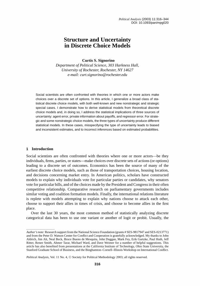
Fig. 1 Four strategic discrete choice models. All of these discrete choice models share the same choicestructure and the same observed utilities, Um(Yk). The only difference is in the source of uncertainty.In (a), there is no uncertainty. In (b), agent error αmj enters through actions at information sets. In (c),each player has private information πmk concerning his or her outcome payoffs. And, in (d), the playersperfectly observe each other’s payoffs, but the analyst does not, resulting in regressor error εmk .

2.1 Choice Model

The choice model identifies not only the set of players, their sequence of moves, their options,and their incentives, but also the rule players use to choose among options. Take Fig. 1aas an example. Here, players 1 and 2 each make one of two choices. Player 1 must choosebetween actions a1 and a2. If a1 is chosen, then outcome Y1 results. If a2 is chosen, thenplayer 2 chooses between actions a3 and a4, resulting in outcomes Y3 and Y4, respectively.

A player’s “true” utility for an action or outcome will often consist of an observablecomponent, related to the explanatory variables, and an unobservable component, relatedto the type of uncertainty. Player m’s true utility for outcome Yk will be written as U ∗

m(Yk).The true utility for an action a j takes the same form: U ∗

m(a j ). We will most often specifythe observable utility component as a linear function of regressors and their associatedparameters, Um(Yk) = Xmkβmk , though this need not always be the case.2 In Fig. 1a, thereis no source of uncertainty, so the true outcome utilities are simply U ∗

m(Yk) = Um(Yk).

2For a given data set, there is an implicit observation index i associated with utilities and error terms. For notationalsimplicity, I will tend to suppress it.

P1: XXX

mpg020 October 6, 2003 8:46


Finally, we need to identify how players choose among different options. In general,we will assume that players choose actions that maximize their expected utility. Formallyspecifying the choice structure and choice rule precisely relates the dependent variable—whether it is an action or outcome in the model—to the explanatory variables, which enterthrough the utilities. With these, we can then identify when actions or outcomes will bechosen (or should be chosen if our model is correct). For example, in Fig. 1a, player 2 willchoose a3 if U ∗

2 (a3) > U ∗2 (a4), and will choose a4 otherwise. Player 1 will choose a1 if

U ∗1 (a1) > U ∗

1 (a2), and will choose a2 otherwise. We can also deduce which outcome resultsin equilibrium:

y =

Y1 if U ∗2 (Y4) > U ∗

2 (Y3) and U ∗1 (Y4) < U ∗

1 (Y1), or

if U ∗2 (Y3) > U ∗

2 (Y4) and U ∗1 (Y3) < U ∗

1 (Y1)

Y3 if U ∗2 (Y3) > U ∗

2 (Y4) and U ∗1 (Y3) > U ∗

1 (Y1)

Y4 if U ∗2 (Y4) > U ∗

2 (Y3) and U ∗1 (Y4) > U ∗

1 (Y1)

. (1)

In words, Y1 will result in two situations: (1) if player 2 prefers Y4 to Y3 but player 1 prefersY1 to Y4, or (2) if player 2 prefers Y3 to Y4 but player 1 prefers Y1 to Y3. Similarly, Y3 willbe the outcome if player 2 prefers Y3 to Y4 and player 1 prefers Y3 to Y1.

With data for the explanatory variables Xmk , we could use the above choice equationsto predict the actions or outcomes that would be chosen. It is important to note that byassuming no uncertainty in the model, we are assuming that the players are perfectly ratio-nal, have complete information, and that we as analysts perfectly observe what comprisestheir utilities. The action and outcome probabilities in Fig. 1a will be degenerate—eitherzero or one—and will correspond to the subgame perfect equilibrium.3 Although this isnot a statistical model, a comparison could be made of the subgame perfect equilibriumpredictions y versus the observed outcomes y.

2.2 Sources of Uncertainty

To conduct statistical analysis, we require a probability model that puts positive probabilityover all outcomes. The random component enters as an assumption about (1) the informationavailable to the analyst concerning the players’ utilities, (2) the information available toeach player concerning the other’s utilities, or (3) both. The first point underscores a majordifference between our undertaking and that of traditional game theorists: game theoristsare omniscient with respect to their models—they know (and specify) each of the players’utilities when they solve for the equilibria. The poor empirical analyst is not so fortunate.We may assume an underlying game-theoretic model. However, we must allow for the factthat we cannot know the players’ true utilities.

In this article, I consider three sources of uncertainty: agent error, private informationabout outcome payoffs, and regressor error.

2.2.1 Agent Error

One source of uncertainty sometimes appealed to in the random utility literature is the“black box” of bounded rationality. It is assumed that players sometimes misperceive each

3Throughout this article, I will assume ties in utilities over outcomes do not occur. In general, the assumption doesnot need to be made on any grounds. In a few cases, it is made for mathematical and pedagogical convenience.

P1: XXX

mpg020 October 6, 2003 8:46


other’s utilities or that they err in implementing their actions.4 Consider Fig. 1b. Agent erroris assumed to enter the model via choices or actions at information sets (i.e., at decisionpoints), rather than through the outcome utilities. Let player m’s true utility for action a j

be U ∗m(a j ) = Um(a j ) + αmj , where αmj represents the error associated with player m’s

action a j . This error term is assumed to be private information to m, so player m knowsher true utility U ∗

m(a j ), but the analyst and other players know only the observable utilitycomponent Um(a j ) and the distribution of αmj . Player m knows that everyone else knows thedistribution of αmj , and so on. Each player’s equilibrium choice probabilities are, therefore,based on her expected utilities, which take into account the fact that everyone else maymake mistakes. Note that this form of uncertainty is purely theoretical—we are making anassumption about what players in the game know about each other’s incentives or actions.Hence, if we assume this as part of our theory, our theoretical model is then a statisticalmodel from the start.

2.2.2 Private Information About Outcome Payoffs

Another theoretical source of uncertainty would be to assume that the players have privateinformation concerning their own outcome payoffs. Figure 1c graphically depicts this typeof uncertainty. Let player m’s true utility for outcome Yk be U ∗

m(Yk) = Um(Yk) + πmk ,where πmk represents the component of player m’s true utility that is private informationto m.5 We assume that player m knows his or her true utility U ∗

m(Yk), but the analyst andother players observe only Um(Yk) and know only the distribution of πmk . Another way ofthinking about this is that the players know m’s average outcome payoff, but realize thatit varies around that average according to some distribution. As in the case of agent error,player m knows that everyone else knows the distribution of πmk , and so on. Each player’sequilibrium choice probabilities are, therefore, based on his or her expected utilities, whichtake into account the uncertainty concerning outcome payoffs. This form of uncertainty isalso purely theoretical and results in a theoretical model that is also statistical.

2.2.3 Regressor Error

The last form of uncertainty pertains not to the players but solely to the analyst. In this case,all of the players perfectly observe each other’s utilities, but the analyst cannot perfectlymodel their utilities with the explanatory variables available. The error term here is similarto that in traditional regression models, where the disturbance is assumed to representintrinsic randomness, omitted variables, or measurement error, but without any of the usualdeleterious consequences. Consider Fig. 1d. Let player m’s true utility for outcome Yk beU ∗

m(Yk) = Um(Yk)+εmk , where εmk represents the component of player m’s true utility thatthe analyst fails to capture with the regressors used to specify Um(Yk). All players observethe true utility U ∗

m(Yk) for every other player. However, the analyst knows (or assumes)only the distribution of εmk . In this case, the underlying theoretical model in Fig. 1d is notstatistical: it is a traditional game of complete information. What translates the theoreticalmodel into a statistical model is an assumption of uncertainty on the analyst’s part.

To recap, agent error αmj and private information πmk are components of our theoreticalmodel: the former allows for nonrational behavior or “accidents,” whereas the latter allows

4Opening the bounded rationality black box is beyond the scope of this article. Instead, I will take the stated formof it as a given and examine the resulting statistical models.

5Because of the notation, πmk is sometimes also referred to as a “payoff disturbance.”

P1: XXX

mpg020 October 6, 2003 8:46


for rational behavior and incomplete information. In contrast, the regressor errorεmk is due tothe analyst’s inability to specify the utilities perfectly. Additionally, the errors are associatedwith different elements of the model and they differ in whether the analyst versus the playerscan observe them. For example, εmk and πmk are associated with outcome payoffs, whileαmj is associated with actions at information sets; πmk and αmj are private information toplayer m, while εmk is unobservable only by the analyst. Finally, we do not have to assumethat only a single source of uncertainty is present. For example, we might theorize that theplayers have private information and, at the same time, suspect that we as analysts have notperfectly specified the “observable” utilities with our regressors. Therefore, a model withboth πmk and εmk terms might be appropriate. For simplicity, however, I will focus on singlesources of uncertainty and the different probability models they produce.

2.3 Likelihood Equation

Given a choice model, a source of uncertainty, and an appropriate distribution for therandom components, we can derive probabilities for the actions and outcomes in the model.Much of Section 4 will be spent doing exactly this for different probit choice models, so Iwill postpone details on deriving the probabilities. For now, I simply note that the choicemodel in combination with an appropriately specified source of uncertainty is enough toguarantee positive probabilities over all outcomes—exactly what we need for statisticalanalysis. The logic behind this can be seen by considering Fig. 1d, where the uncertaintyis due to regressor error. We previously saw that Y4 is the outcome when U ∗

2 (Y4) > U ∗2 (Y3)

and U ∗1 (Y4) > U ∗

1 (Y1). Substituting for the true utilities, an equivalent statement is that Y4

occurs when U2(Y4) + ε24 > U2(Y3) + ε23 and U1(Y4) + ε14 > U1(Y1) + ε11. As analysts,we do not observe the εmk , so we cannot say with certainty whether the condition is satisfiedor not. All we can do is state the probability that Y4 will occur:

pY4 = Pr[U2(Y4) + ε24 > U2(Y3) + ε23, U1(Y4) + ε14 > U1(Y1) + ε11].

Given an appropriately specified εmk , we can derive the probability that Y4 occurs. TheUm(Yk) are functions of our explanatory variables, for example, Xmkβmk . Therefore, theoutcome probability relates the dependent variable to the explanatory variables and incor-porates the structure of the choice model. Probabilities for the other outcomes, Y1 and Y3,are derived in a similar manner, as are the probabilities for the actions available to eachplayer. In Fig. 1b–1d, the probability of action a j is denoted as p j .

With these action and outcome probabilities, we can construct a likelihood function forour dependent variable. Assume the probabilities have been derived for one of the models inFig. 1b–1d. Consider the situation where our dependent variable represents which outcomeoccurred. Let δk = 1 if outcome Yk occurred in the current observation, and zero otherwise.Then the likelihood function is

L =N∏

pδ1Y1

pδ3Y3

pδ4Y4

. (2)

The outcome probabilities are functions of the explanatory variables and effects parameters.Therefore, the maximum likelihood estimates can be found by maximizing Eq. (2) withrespect to the parameters—and standard statistical tests (e.g., t or likelihood ratio) can beconducted.

If our dependent variable instead consists of actions taken by a player, then we wouldconstruct a similar likelihood function, but with the corresponding action probabilities.

P1: XXX

mpg020 October 6, 2003 8:46


For example, for a dependent variable denoting whether a1 or a2 occurred, the likelihoodfunction would be

L =N∏

pδa11 p

δa22 , (3)

where δa j = 1 if action a j was chosen, and zero otherwise. The reader familiar with tra-ditional binomial and multinomial choice models will note that Eqs. (2) and (3) share thesame general form as in multinomial logit and probit. However, the probabilities pYk and p j

incorporate the choice structure of our theory, which may differ from nonstrategic binomialand multinomial choice structures.

3 A General Class of Statistical Discrete Choice Models

The class of models in this section generalizes those statistical discrete choice models inextensive form that allow for agent error, private information about payoffs, and regressorerror. Although it is based on a general specification of an extensive form game, it does notrequire that the model be strategic. In words, we first need to define the choice tree, thenassign players, information sets, actions, and outcomes to the nodes of that tree, then assignutilities to the actions and outcomes, then specify the distribution of the errors associatedwith utilities over actions and outcomes, and, finally, specify the rule players use to makedecisions. The notation can be dense at times. However, the core ideas are exactly the sameas those just outlined. Concrete examples of these will be given in Section 4.

3.1 Choice Tree

The discrete choice tree is specified as a set of nodes with an asymmetric precedencerelation defined over the nodes. Let Q be the set of all nodes, with q0 the initial node. Let≺ be an asymmetric precedence relation, such that q ≺ q ′ if node q immediately precedesnode q ′, and q ′ � q if node q ′ immediately follows q. For a node q, define the set of itsimmediate successor nodes as S(q) = {q ′ | q ≺ q ′} and define a terminal node qt as onewhere S(qt ) = ∅. Define the set of terminal nodes as Qt . A path P(qt ) from the initialnode q0 to a terminal node qt is a sequence of nodes (q0, . . . , qt ) that connects q0 to qt

such that for each nonterminal node in the sequence, the following node is its immediatesuccessor. All paths are assumed to be countably finite. This rules out games such as aninfinitely repeated prisoner’s dilemma.

3.2 Information Sets

Let M be the set of players. Define the information set containing node q and assigned toplayer m as ιm(q). Define the set of information sets assigned to player m as Im and the set ofall information sets as I = ⋃

m Im . As all information sets considered here are singletons,it will sometimes be less notationally cumbersome to refer to an information set simply bythe single node assigned to it.

3.3 Actions and Outcomes

Let a(q) be the label for the action (or option) required to reach q from its predecessor, letA(q) = {a(q ′) | q ′ ∈ S(q)} be the set of all actions available at q for the player assignedto q , and let A = ⋃

q A(q) be the set of all actions in the game. Define g : Qt → Y as thefunction that maps terminal nodes Qt to outcomes Y . Outcomes are simply labels assigned

P1: XXX

mpg020 October 6, 2003 8:46


to terminal nodes. Although different paths must by definition lead to different terminalnodes, they can result in the same outcome. For example, in a crisis model, there may bemultiple paths to war.

3.4 Utilities and “Error” Terms

Utilities are defined similarly to those of traditional random utility models and statisticalequilibrium models.6 However, here we will specify in detail the types of uncertainty thatcan enter into the model. Although the utilities and error terms may vary over observationsin a data set, I will continue to suppress the observation index to reduce notation.

For terminal node qtj mapped to outcome Yk , we can alternatively speak of m’s true

utility U ∗m(Yk) for outcome Yk or of m’s true utility U ∗

m[a(qtj )] for the action a(qt

j ) leadingto the outcome Yk assigned to node qt

j . Let player m’s true utility U ∗m(Yk) of outcome Yk be

U ∗m(Yk) = Um(Yk) + εmk + πmk . (4)

Here, Um(Yk) is the observable component of m’s utility for outcome Yk—for example,as a function of explanatory variables Xmk and effects parameters βmk . It is assumed thatthe analyst and all players observe Um(Yk). εmk is the portion of the true utility that isnot captured by the regressors. We assume each player observes the εmk of every otherplayer, but the analyst cannot observe εmk (otherwise he or she would have included it inthe regressors). πmk is the portion of m’s true utility that is private to m. Neither the analystnor the other players observe player m’s πmk .

For nonterminal node q j , let player m’s true utility U ∗m[a(q j )] for choosing action a(q j )

be defined as

U ∗m[a(q j )] = Um[a(q j )] + αmj , (5)

where Um[a(q j )] is m’s expected utility for reaching node q j and αmj represents agent errorassociated with action a(q j ). Again, αmj is assumed known only by player m.

3.5 Distribution of Errors

Let εm be the vector of m’s regressor error terms and let ε = (ε1, . . . , ε#M ) be the vector ofevery players’ regressor errors.7 Similarly, let πm be the vector of m’s payoff disturbancesover each of her utilities and let π = (π1, . . . , π#M ) be the vector of every players’ payoffdisturbances. Finally, let αm be the vector of player m’s agent errors over each of his or heractions and let α = (α1, . . . ,α#M ) be the vector of every agent’s errors. For mathematicalconvenience, let ε, π, and α be distributed according to the same continuous joint densityfunction f (·). Denote the combined error vector as � = (ε, π, α).

3.6 Agent Utility Maximization

A multiagent representation is assumed.8 A player is represented by an “agent” at eachinformation set who shares the player’s payoff function but makes decisions independently

6For random utility models, see McFadden 1974a, 1974b, 1976; Hausman and Wise 1978. For statistical equi-librium models, see McKelvey and Palfrey 1996, 1998; Chen et al. 1996; Zauner 1996.

7The notation #S is used to denote the number of elements in the set S.8This is also referred to as “agent normal form” or “agent strategic form.”

P1: XXX

mpg020 October 6, 2003 8:46


of the other agents. At each information set ιmj (q), the agent for player m chooses theaction a(q ′) that maximizes her utility from that node in the tree: U ∗

m[a(q ′)] > U ∗m[a(q ′′)]

∀a(q ′′) = a(q ′) ∈ A(q). Consequently, an equilibrium strategy must be in the interest ofevery agent, even off the equilibrium path.

3.7 Statistical Discrete Choice Model

Given the above, the tuple (Q, ≺, M, I, A, Y, U, �) defines a statistical discrete choicemodel with well-defined choice probabilities over each action and, hence, over each out-come.

Define the probability of outcome Yk as

pYk = Pr[Yk]

=∑

{qt |g(qt )=Yk }Pr[P(qt )]. (6)

If only one terminal node qt is assigned to a particular outcome Yk , then Eq. (6) is pYk =Pr[P(qt )], the joint probability of realizing each of the actions on the path P(qt ). If the sameoutcome is assigned to multiple terminal nodes, then Eq. (6) is the sum of the probabilitiesof realizing each of those paths leading to the different terminal nodes {qt | g(qt ) = Yk}mapped to the same outcome.

Assume now that we have N observations of a dependent variable y that takes on thevalues yi ∈ Y . Define j ∈ Y and let the dummies yi, j take on the value

yi, j ={

1 if j = yi

0 otherwise.

In other words, yi, j is a dummy that indicates whether outcome j occurred or not in ob-servation i . Assuming that the utilities are specified in terms of explanatory variables (e.g.,Umki (Yk) = Xmkiβmk), then we can denote the probability of Yk occurring in observa-tion i as pYk i and estimate the parameters βmk by maximizing the multinomial likelihoodfunction

L =N∏

i=1

∏j∈Y

pyi, j

j i (7)

with respect to the βmk . Again, Eq. (7) should not be interpreted as representing a multino-mial logit or probit model. Rather, the data vector y has a multinomial distribution. Whetherthe model implied by the tuple (Q, ≺, M, I, A, Y, U, �) is multinomial logit or probit, bi-nomial logit or probit, a sequential model, a strategic model—or something else entirelydifferent—will depend on the elements of the tuple. I now turn to these special cases.

3.8 Special Cases

The general model has a number of well-known, as well as new, special cases, depending onwhat we substitute for the elements of the tuple (Q, ≺, M, I, A, Y, U, �). Table 1 displaysa number of these special cases, which are defined based on the number of players #M ,the number of information sets #I , the number of terminal nodes #Qt , the number of

P1: XXX

mpg020 October 6, 2003 8:46


Table 1 Special cases of the general statistical discrete choice modeldefined by the tuple (Q, ≺, M, I, A, Y, U, �).

Special casesPlayers

M

Infosets

I

Terminalnodes

QtOutcomes

Y � ∼ TlEV � ∼ N(0, �)

Nonstrategic

1 1 2 2 Binomial Binomiallogit probit

1 1 ≥2 #Qt Multinomial Multinomiallogit probit

Nested logita

1 >1 >#I >1 Sequential Sequentiallogit probit

1 or 2 2 3 3 Heckmanselection

Strategic

>1 ≥#M >#I >1 Logit Probit

Note. The general model includes a number of well-known, as well as new, statisticalmodels, depending on what we substitute for the elements of the tuple. The specialcases in the table are defined based on the number of players #M , the number ofinformation sets #I , the number of terminal nodes #Qt , the number of outcomes #Y ,and whether the errors have type 1 extreme value or normal distributions. Withinthe class of strategic models are further special cases that depend on which sourcesof uncertainty are present: agent error, private information, regressor error, or somecombination of the three.a� ∼ GEV.

outcomes #Y , and whether the errors � = (ε, π, α) have type 1 extreme value or normaldistributions.

For example, the main difference between nonstrategic and strategic models is that theformer usually have only a single decision maker (#M = 1), while the latter have multipleplayers (#M > 1). Within the nonstrategic models, the main source of differentiation is thenumber of terminal nodes and the number of information sets. Binomial logit/probit hasonly one information set and is a special case of multinomial logit. These are differentiatedfrom sequential logit/probit, which have multiple information sets. Heckman-type selectionmodels may have either one or two players. Although not shown in Table 1, as we will see inSection 4, different sequential models also arise depending on our assumptions concerningwhether a player’s agents have private information concerning their disturbances relativeto other agents of the same player (more on this later).

With the strategic models, we assume there are multiple players, at least one informationset for each player, and more terminal nodes than information sets. This last assumptionensures that we have at least a binary decision by each player. There are a number ofexisting and new special cases within the “strategic” class. For example, the logit quan-tal response equilibrium (QRE) of McKelvey and Palfrey (1998) is the special case withagent errors that are independently distributed type 1 extreme value. A statistical equilib-rium model with independently normally distributed agent errors would be equivalent to aprobit version of the QRE. Signorino (2002) analyzes a model with normally distributedagent errors that are correlated between two players, synthesizing aspects of traditional

P1: XXX

mpg020 October 6, 2003 8:46


Heckman selection models and QRE-based strategic models. The statistical equilibriummodel in Zauner (1996) involves normally distributed payoff perturbations.9 With the ex-ception of Signorino (1999, 2002) and Signorino and Yilmaz (2003), none of these havebeen developed for use in regression analysis. Finally, these are just a few of the specialcases of the general model. Any number of other models are possible, depending on theassumptions concerning which types of uncertainty are present, the observability of thedisturbances by the analyst and players, and the distribution and covariance structure of thedisturbances.

4 Examples: Probit Choice Models

The models generalized in Section 3 are illustrated using three examples: (1) nonstrategicnonsequential choice models, (2) nonstrategic sequential choice models, and (3) strategicchoice models. Although the first has been addressed in detail elsewhere under the rubric of“discrete choice” (see McFadden 1974a, 1974b, 1976; Hausman and Wise 1978; Maddala1983; Pudney 1989) and the second has also received some (albeit much less) attention,all three are useful for demonstrating not only how one would apply the general modelto specific applications, but also how the choice and outcome probabilities relate to thecharacteristics of the tuple (Q, ≺, M, I, A, Y, U, �). In fact, the three models provide anice progression concerning those characteristics.

Throughout this section, I will assume that errors are normally distributed. Therefore,the discrete choice models examined here will be nonstrategic and strategic probit models.For a given discrete choice model, I show how it relates to the general model and how toderive the choice probabilities.

4.1 Nonstrategic Nonsequential Choice

The simplest nontrivial discrete choice model is that depicted in Fig. 2a, where a single de-cision maker (labeled 1) must choose between #Y = 2 outcomes. Examples might includewhether a state votes for a United Nations resolution, whether a citizen votes Democrator Republican, or whether a commuter takes the bus to work or drives. The tree is definedby the set of nodes Q = {q0, q1, q2} and the precedence relation among them: q0 ≺ q1

and q0 ≺ q2. The terminal nodes Qt = {q1, q2} are mapped to outcomes Y = {Y1, Y2}.There is only a single information set ι1(q0). The action required to reach node q j isdenoted by a j . The observation index i will be suppressed unless it is required to high-light that the dependent variable, explanatory variables, utilities, or probabilities vary overobservations.

The theoretical story for regressor error ε and payoff disturbances π is identical here.What usually differentiates them is that ε is observed by all players, while π is privateinformation. As there is only one decision maker, both represent part of a perfectly rationaldecision maker’s utility that is unobserved by the analyst. The story for agent error α isslightly different in that α is assumed to arise because of misperception or implementationerror on the decision maker’s part. Nevertheless, regardless of the underlying theoreticalstory for the uncertainty, the resulting statistical models estimated will be identical, as thechoice structure in Fig. 2a contains only a single information set.

9Zauner (1996) develops a two-sided incomplete information model with normally distributed payoff disturbancesfor the analysis of experimental data from the centipede game, but where payoffs are fixed and only the varianceis estimated.

P1: XXX

mpg020 October 6, 2003 8:46


0

1 2

p1 p2

1

a1 a2

U1*(Y1) U1

*(Y2)

0

1

p1 p2

1

2

3 4

p3 p4

1

a1 a2

a3 a4U1*(Y1)

U1*(Y3) U1

*(Y4)

0

1

p1 p2

1

2

3 4

p3 p4

2

a1 a2

a3 a4U1*(Y1)

U1*(Y3)

U2*(Y3)

U1*(Y4)

U2*(Y4)

(a) Nonstrategic Nonsequential Choice

(c) Strategic Choice

(b) Nonstrategic Sequential Choice

Fig. 2 Discrete choice examples. Parts (a) and (b) are nonstrategic choice models, consisting of asingle decision maker. Parts (b) and (c) are sequential choice models. Part (c) is a strategic choicemodel, where player 1 must condition his or her choice on what he or she expects player 2 will do.Options are denoted by a j , choice probabilities as p j , outcomes as Yk , and player m’s utility foroutcome Yk as U ∗

m(Yk).

To see this, consider that the utilities in each case areRegressor error:

U ∗1 (Yk) = U1(Yk) + εk (8)

Private information about outcome payoffs:

U ∗1 (Yk) = U1(Yk) + πk (9)

Agent error:

U ∗1 (ak) = U1(ak) + αk

= U1(Yk) + αk . (10)

A utility-maximizing decision maker will choose Y1 if U ∗1 (Y1) > U ∗

1 (Y2). Assuming thedisturbances are normally distributed with mean zero and covariance structure � = [ σ2

1σ12 σ2

2],

P1: XXX

mpg020 October 6, 2003 8:46


then in the regressor error case,

pY1 = Pr[U ∗1 (Y1) > U ∗

1 (Y2)]

= Pr[U1(Y1) + ε1 > U1(Y2) + ε2]

= Pr[ε2 − ε1 < U1(Y1) − U1(Y2)]

= �

U1(Y1) − U1(Y2)√

σ21 + σ2

2 − 2σ12

(11)

where �(x) is the standard normal distribution. The probability that the decision maker willchoose option Y2 is simply pY2 = 1 − pY1 .

It is easy to see that the probabilities will be exactly the same (under the same conditions)for the agent error and private information models. Hence, given the same structural andcovariance assumptions, the three forms of uncertainty lead to observationally equivalentstatistical models.

4.2 Nonstrategic Sequential Choice

This section serves as a bridge between the nonstrategic models and the strategic mod-els. On the one hand, the sequential models presented in this section are all nonstrate-gic and, as we will see, at times reduce to nonsequential models. On the other hand, thesequence of decisions, observability of error terms, and calculations of expected utilityenter into the sequential models’ choice probabilities in much the same way as they dofor the strategic models. Depending on the assumptions, the choice probabilities in thissection tend to be similar either to those of the previous section or to those of the nextsection.

Figure 2b displays a situation where a single decision maker (labeled 1) makes sequentialchoices over actions leading to #Y = 3 outcomes. First, he or she must choose betweenaction a1 and a2. If a2 is chosen, then he or she must choose between a3 and a4. The treeis defined by the set of nodes Q = {q0, q1, q2, q3, q4} and the precedence relation amongthem: q0 ≺ q1, q0 ≺ q2, q2 ≺ q3, and q2 ≺ q4. The terminal nodes Qt = {q1, q3, q4} aremapped to outcomes Y = {Y1, Y3, Y4}. There are two information sets: ι1(q0) and ι1(q2).The action required to reach node q j is denoted by a j . Decision maker 1 has utilities U ∗

1 (Y1),U ∗

1 (Y3), and U ∗1 (Y4) for the three outcomes.


In this case, the decision maker is perfectly rational and perfectly observes the utilities, butthe analyst does not observe part of the variation in the utility. Hence, U ∗

1 (Yk) = U1(Yk)+εk .To calculate pYk , we must first determine the conditions for Yk to be realized. Given theabove assumptions, the following identifies the conditions for each of the outcomes tooccur:

y =

Y1 if U ∗1 (Y1) > U ∗

1 (Y3) and U ∗1 (Y1) > U ∗

1 (Y4)

Y3 if U ∗1 (Y3) > U ∗

1 (Y4) and U ∗1 (Y3) > U ∗

1 (Y1)

Y4 if U ∗1 (Y4) > U ∗

1 (Y3) and U ∗1 (Y4) > U ∗

1 (Y1)

. (12)

P1: XXX

mpg020 October 6, 2003 8:46


As we do not perfectly observe the true utilities, we can only make probabilistic statementsconcerning the outcomes. So, for example, the probability pY1 of Y1 occurring in observationi is

pY1 = Pr[U1(Y1) + ε1 > U1(Y3) + ε3, U1(Y1) + ε1 > U1(Y4) + ε4]. (13)

Assuming that (ε1, ε3, ε4) ∼ N (0, �ε), with

�ε =σ2

ε1

σε13 σ2ε3

σε14 σε34 σ2ε4

(14)

and letting η31 = ε3 − ε1 and η41 = ε4 − ε1, then Eq. (13) can be rewritten as

pY1 = Pr[η31 < U1(Y1) − U1(Y3), η41 < U1(Y1) − U1(Y4)]

=∫ U1(Y1)−U1(Y3)

−∞

∫ U1(Y1)−U1(Y4)

−∞φ(η31, η41) dη41 dη31 (15)

where φ(η31, η41) is the bivariate normal density with mean zero and variance

�η =[

σ2ε1

+ σ2ε3

− 2σε13

σ2ε1

− σε13 − σε14 + σε34 σ2ε1

+ σ2ε4

− 2σε14

]. (16)

The reader will notice that this is equivalent to the traditional multinomial probit probabilityof choosing outcome Y1 from the set Y = {Y1, Y3, Y4}—that is, where there is only asingle information set and three outcomes (see, e.g., Hausman and Wise 1978; Alvarez andNagler 1998). The probabilities of choosing Y3 and Y4 yield similar multinomial probitprobabilities. Therefore, with a single perfectly rational decision maker and only regressorerror, the sequence of choices are irrelevant, and the statistical model is observationallyequivalent to a nonstrategic nonsequential model with the same number of options and thesame covariance structure.


In Section 4.1, we saw that with only a single information set, payoff disturbances yieldednot only the same statistical model as with regressor error, but also the same underlyingstory: they represent variation in outcome utilities that the decision maker observes, but theanalyst does not. With multiple information sets, that may or may not be the case, dependingon our assumption of whether payoff disturbances are observable by all “agents” of the sameplayer.

In the typical multiagent model (see Myerson 1991, p. 61; Osborne and Rubinstein1994, p. 250), each player is represented at each information set by a different agent, whohas the same preferences as the player and makes a decision for the player. In the currentcontext, the usual multiagent representation would assume that every agent of a given playerobserves the disturbances of the other agents of the same player, as they all share the samepreferences.

P1: XXX

mpg020 October 6, 2003 8:46


A variation on this is to assume that the error terms are private information for eachindividual agent of the player. In other words, each agent of the player observes her owndisturbance, but does not observe the error terms of the other agents.10 Why might we dothis, given that there is really only a single decision maker? Simply put, decision makersmay not know what their true payoffs are “down the road,” or, in the agent error models,what errors they might make in future decisions. It may make more sense then to assumethat a player perceives her outcome payoff differently at different points in the game orthat the agent error associated with actions at an information set is observable only by theagent at that information set. Under these assumptions, an agent must form an expectedutility for an action that leads to another information set, even when that information set isassigned to the same player the agent represents. Examples of both the standard multiagentrepresentation and this variation are given in the following.

In the case where the decision maker’s agents observe each other’s payoff disturbances,the problem is identical to one of regressor error: the decision maker is perfectly rational, theonly uncertainty is on the analyst’s part, and the uncertainty is with respect to the outcomeutilities. The sequence of choices is irrelevant. If we assume that the payoff disturbances arenormally distributed, then the resulting choice probabilities are the same multinomial probitprobabilities we derived in the regressor error case. Both are observationally equivalent witha nonstrategic nonsequential model with any type of error, assuming the same outcomes,utilities over outcomes, and distribution of errors.

This is not the case when the payoff disturbances are private information to each agent ofa player. In fact, this situation is equivalent to a game with multiple players, who all share thesame observable utility components Um(Yk), but have different payoff disturbances πmk .11

The probability that player 1 chooses outcome Y4 is the probability Pr[P(q4)] that the pathP(q4) is realized, which is the joint probability of the decisions along it being realized.Denote by p j the probability that action a j is chosen at the parent information set of a j .If we assume that the payoff disturbances are independent of each other, then the jointprobability is just the product of the two individual choice probabilities p2 and p4.12 Tocalculate the choice probabilities, we will work up the tree, as decisions made at informationsets earlier in the tree are based on expected utilities that require choice probabilities foractions later in the tree.

As we do not observe the payoff disturbances, the probability p4 that the agent at infor-mation set ι1(q2) chooses a4 is

p4 = �

U1(Y4) − U1(Y3)√

σ2π3

+ σ2π4

. (17)

The probability p2 that the agent at information set ι1(q0) chooses a2 must be written in termsof her expected utility for choosing action a2, which is U ∗

1 (a2) = p3U ∗1 (Y3) + p4U ∗

1 (Y4).

10Although not expressed in exactly the same way as presented here, nonstrategic “decentralized” sequentialchoice models share this feature (see, e.g., Pudney 1989, pp. 122–130).

11Technically, we should let the true outcome utility of player m’s agent n at information set ιm (qn) be denoted byU∗

1n(Yk ) = U1(Yk ) + π1n k . Because this notation is cumbersome, I will not index agents of players. However,

the reader should keep in mind that the true utilities and error terms are implicitly indexed this way under theassumption of multiple agents with private errors.

12I will hereafter assume that errors are independently distributed; hence, all covariances are zero. This is madepurely to simplify the math. However, it does have other implications that we will return to later.

P1: XXX

mpg020 October 6, 2003 8:46


The agent’s probability of choosing a2 is then

p2 = Pr[U ∗1 (a2) > U ∗

1 (a1)]

= Pr[p3U ∗1 (Y3) + p4U ∗

1 (Y4) > U ∗1 (Y1)]

= Pr [p3 [U1(Y3) + π3] + p4 [U1(Y4) + π4] > U1(Y1) + π1]

= �

p3U1(Y3) + p4U1(Y4) − U1(Y1)√

p23σ

2π3

+ p24σ

2π4

+ σ2π1

. (18)

Choice probabilities p3 and p1 are, of course, 1 − p4 and p1 = 1 − p2, respectively.Because the error terms are assumed independent, the outcome probabilities simplify to

pY1 = p1 (19)pY3 = p2 p3 (20)pY4 = p2 p4. (21)

These are clearly not the multinomial probit probabilities we saw in the regressor error case.The probability of Y1 here is

pY1 = �

U1(Y1) − [p3U1(Y3) + p4U1(Y4)]√

p23σ

2π3

+ p24σ

2π4

+ σ2π1

. (22)

In contrast to the multinomial probit’s joint comparison of U1(Y1) against both U1(Y3) andU1(Y4), here the sequential choice is reflected in the numerator of Eq. (22) by the com-parison of U1(Y1) to a weighting of U1(Y3) and U1(Y4), where the weighting is based onthe probability that the respective outcomes will be selected. This is directly a result ofthe agent at information set i1(q0) having to form an expected utility concerning actiona2 because of her uncertainty concerning her decision at i1(q2). Second, notice that whilethe multinomial probit probabilities have a constant variance in their denominators, herethe variance in the denominator contains probabilities (e.g., p3 and p4) that will vary overthe observations (as they are functions of utilities that are themselves functions of explana-tory variables that will vary over observations).

4.2.3 Agent Error

I consider only the case where agent error over actions at a particular information set isprivate information to the agent at that information set. The derivation of the outcomeprobabilities proceeds similarly to those in the model with private payoff disturbances.

As we do not observe the agent error, the probability p4 that the agent at information setι1(q2) chooses a4 is

p4 = �

U1(Y4) − U1(Y3)√

σ2α3

+ σ2α4

. (23)

The probability p2 that the agent at information set ι1(q0) chooses a2 must be written interms of her expected utility for choosing action a2. Since the error term comes in through

P1: XXX

mpg020 October 6, 2003 8:46


actions rather than outcomes, the expected utility is slightly different than with the payoffdisturbances model:

U ∗1 (a2) = U1(a2) + α2

= [p3U1(a3) + p4U1(a4)] + α2. (24)


p2 = Pr[U ∗1 (a2) > U ∗

1 (a1)]

= Pr[p3U1(a3) + p4U1(a4) + α2 > U1(a1) + α1]

= Pr [p3U1(Y3) + p4U1(Y4) + α2 > U1(Y1) + α1]

= �

p3U1(Y3) + p4U1(Y4) − U1(Y1)√

σ2α1

+ σ2α2

. (25)

The outcome probabilities take the same general form as Eqs. (19)–(21), but substitutingthe agent error versions of the p j action probabilities.

As with private payoff disturbances, these are clearly not multinomial probit probabilities.Here, the probability of Y1 occurring is

pY1 = �

U1(Y1) − [p3U1(Y3) + p4U1(Y4)]√

σ2α1

+ σ2α2

. (26)

This is somewhat similar to the corresponding probability in the (agent–private) payoffdisturbance case. However, there the outcome probabilities contained variance terms thatvaried over observations, whereas here the variance terms [in the denominator of Eq. (26)]are constant across observations.

The import of this section has been to show that the type of uncertainty specified by thetheoretical model can matter in the resulting statistical model. Although the nonstrategicnonsequential choice models produced observationally equivalent statistical models, thesequencing of decisions and the assumptions concerning uncertainty resulted in a numberof different statistical models here. As we will see, the same holds true for the strategicmodels, to which we now turn.

4.3 Strategic Choice

The new element introduced in this section is that there are now not just multiple agents ofa single decision maker, but multiple decision makers, each of whom must condition theirbehavior on the expected behavior of the others. The probabilities are therefore consideredequilibrium choice probabilities. We have actually already seen one simple example of this.A nonstrategic sequential choice model, where disturbances are assumed private informationto each agent, can be viewed as a strategic model where each agent is a different decisionmaker but all decision makers share the same observed outcome utilities Um(Yk). Thenonstrategic choice probabilities in the former are the equilibrium choice probabilities ofthe latter.

Figure 2c, which displays a strategic discrete choice model in extensive form, will beused as the referent example throughout this section. Here, we have two decision makers

P1: XXX

mpg020 October 6, 2003 8:46


(labeled 1 and 2) who make choices in turn. Player 1 must choose between action a1 and a2.If a2 is chosen, then player 2 must choose between a3 and a4. The tree is defined by the set ofnodes Q = {q0, q1, q2, q3, q4} and the precedence relation among them: q0 ≺ q1, q0 ≺ q2,q2 ≺ q3, and q2 ≺ q4. The terminal nodes Qt = {q1, q3, q4} are mapped to outcomesY = {Y1, Y3, Y4}. There are two information sets: ι1(q0) and ι2(q2). The action required toreach node q j is denoted by a j . Decision maker m has utility U ∗

m(Yk) for outcome Yk .


Again, we assume that both players are perfectly rational and view each other’s payoffsperfectly, but we (the analysts) do not observe part of the variation in the utility. Hence,U ∗

m(Yk) = Um(Yk) + εmk . As in the sequential model, to calculate pYk , we ask ourselves:What are the conditions for Yk to be realized? With perfectly rational players, who have com-plete information about each other’s utilities and make decisions at singleton informationsets, that question is equivalent to asking when Yk will be the subgame perfect equilibrium(SPE) outcome in Fig. 2c.

Without any constraints on the preferences over outcomes, a general specification of theSPE conditions can be quite tedious for more complicated models. However, for the modelin Fig. 2c, the conditions are not terribly cumbersome. The SPE is

y =

Y1 if U ∗2 (Y3) > U ∗

2 (Y4) and U ∗1 (Y1) > U ∗

1 (Y3) or

if U ∗2 (Y4) > U ∗

2 (Y3) and U ∗1 (Y1) > U ∗

1 (Y4)

Y3 if U ∗2 (Y3) > U ∗

2 (Y4) and U ∗1 (Y3) > U ∗

1 (Y1)

Y4 if U ∗2 (Y4) > U ∗

2 (Y3) and U ∗1 (Y4) > U ∗

1 (Y1)

. (27)

As we do not perfectly observe the true utilities, we can only make probabilistic statementsconcerning the outcomes. So, for example, the probability of Y1 occurring is

pY1 = Pr[U ∗2 (Y3) > U ∗

2 (Y4), U ∗1 (Y1) > U ∗

1 (Y3)]

+ Pr[U ∗2 (Y4) > U ∗

2 (Y3), U ∗1 (Y1) > U ∗

1 (Y4)]

= Pr[U2(Y3) + ε23 > U2(Y4) + ε24, U1(Y1) + ε11 > U1(Y3) + ε13]

+ Pr[U2(Y4) + ε24 > U2(Y3) + ε23, U1(Y1) + ε11 > U1(Y4) + ε14]. (28)

Denote the variance of εi j as σ2εi j

and the covariance of εi j with εik as σεi jk . If we letηi jk = εi j − εik , then we can rewrite Eq. (28) as

pY1 = Pr[η243 < U2(Y3) − U2(Y4), η131 < U1(Y1) − U1(Y3)]

+ Pr[η234 < U2(Y4) − U2(Y3), η141 < U1(Y1) − U1(Y4)]

=∫ U2(Y3)−U2(Y4)

−∞

∫ U1(Y1)−U1(Y3)

−∞φ(η243, η131) dη131 dη243

+∫ U2(Y4)−U2(Y3)

−∞

∫ U1(Y1)−U1(Y4)

−∞φ(η234, η141) dη141 dη233. (29)

Both terms in Eq. (29) require integration over standardized bivariate normal densities.Given modern computing, this is not difficult. However, if we assume that the disturbances

P1: XXX

mpg020 October 6, 2003 8:46


are independent of each other, then the equation further simplifies to

pY1 = �

U2(Y3) − U2(Y4)√

σ2ε23

+ σ2ε24

�

U1(Y1) − U1(Y3)√

σ2ε11

+ σ2ε13

+ �

U2(Y4) − U2(Y3)√

σ2ε24

+ σ2ε23

�

U1(Y1) − U1(Y4)√

σ2ε11

+ σ2ε14

. (30)

Carrying out the same steps to calculate pY3 and pY4 gives

pY3 = �

U2(Y3) − U2(Y4)√

σ2ε23

+ σ2ε24

�

U1(Y3) − U1(Y1)√

σ2ε13

+ σ2ε11

(31)

pY4 = �

U2(Y4) − U2(Y3)√

σ2ε23

+ σ2ε24

�

U1(Y4) − U1(Y1)√

σ2ε14

+ σ2ε11

. (32)

Examining Eqs. (30)–(32), a number of issues are immediately apparent. First, com-paring the above equations to the similar nonstrategic sequential choice Eqs. (12)–(15),we see that the strategic probability model is not a multinomial probit model, as in thenonsequential case with regressor error, even when we assume the disturbances are inde-pendent. Eqs. (30)–(32) reflect the observable utilities of two players, not one. In particular,the equilibrium conditions for outcome Y1 are quite different in the two models, leading todifferent probability models. Therefore, if the data-generating process is the game shownin Fig. 2c and if the players have perfect and complete information, then employing any ofthe nonstrategic models will result in specification error.

Second, it was relatively easy to specify the equilibrium conditions and derive the prob-ability model for the game shown in Fig. 2c. However, this becomes increasingly difficultas the complexity of the game increases. In fact, one does not need to add many moreinformation sets for the specification to become much more involved.

Third, and related, the complexity of the underlying game will affect the dimensionalityof the integration required for the equilibrium probabilities. In Fig. 2c, each player makesonly a single decision. The sequence of choices results in bivariate normal densities, andthe independence assumption allows us to write the equilibrium probabilities in terms ofunivariate normal cdf’s. However, even if we assume the εmk disturbances are independent,more complex games (e.g., with more information sets) will result in probability modelswith multivariate normal densities of higher dimension, which could be computationallyintensive. This is an issue not just of the number of choices at information sets (e.g., asin multinomial probit), but also of the depth of the game tree—specifically, the number oftimes a player makes decisions down a particular path.


We now assume that a decision maker m’s outcome utilities are private information: theanalyst and other players know (or assume) only the distribution of m’s outcome payoffs.Additionally, for the payoff disturbance and agent error models, we will continue to assume

P1: XXX

mpg020 October 6, 2003 8:46


the multiagent representation discussed in Section 4.2, where disturbances are private in-formation to each individual agent, and where the disturbances are independent of eachother.

To derive the choice probabilities, we will work “up the tree.” The choice probabilitiesin the strategic model are derived in a similar manner to those in the nonstrategic sequentialmodel. The probability of action a4 is

p4 = �

U2(Y4) − U2(Y3)√

σ2π24

+ σ2π24

. (33)

Because player 1 is uncertain about player 2’s payoffs, she must assess the probabilitythat player 2 will choose a3 versus a4, and then use that probability in her expected utilitycalculations for her own options. The probability p2 that player 1 chooses a2 is

p2 = Pr[U ∗1 (a2) > U ∗

1 (a1)]

= Pr[p3U ∗1 (Y3) + p4U ∗

1 (Y4) > U ∗1 (Y1)]

= �

p3U1(Y3) + p4U1(Y4) − U1(Y1)√

p23σ

2π13

+ p24σ

2π14

+ σ2π11

. (34)

Because of the independence assumption, the outcome probabilities are the product of theaction probabilities along their paths: pY1 = p1, pY3 = p2 p3, and pY4 = p2 p4.

Notice that the structure of the model can be seen in (1) the expected utility comparison inthe numerator of Equation 34, and (2) the form of the outcome probabilities. Additionally, theequilibrium probabilities above are very similar to the nonstrategic sequential probabilitiesunder the assumption of independent agents. The difference between the two is that theequilibrium probabilities here are a function of two players’ preferences, which the analystwill likely specify with different sets of regressors.

4.3.3 Agent Error

We now assume that players are boundedly rational. As in the previous case, to determinethe strategic probit equilibrium outcome probabilities, we will proceed by first deriving theequilibrium action probabilities.

The probability p4 that player 2 chooses action a4 is

p4 = Pr[U2(Y4) + α24 > U2(Y3) + α23]

= �

U2(Y4) − U2(Y3)√

σ2α23

+ σ2α24

. (35)

The probability p2 that player 1 chooses a2 must be written in terms of her expected utilityfor choosing action a2. As the error term comes in through actions rather than outcomes,the expected utility is slightly different than with the payoff disturbances model:

U ∗1 (a12) = U1(a12) + α12

= [p3U1(a3) + p4U1(a4)] + α12. (36)

P1: XXX

mpg020 October 6, 2003 8:46



p2 = Pr[U ∗1 (a2) > U ∗

1 (a1)]

= Pr[p3U1(a3) + p4U1(a4) + α2 > U1(a1) + α1]

= �

p3U1(Y3) + p4U1(Y4) − U1(Y1)√

σ2α1

+ σ2α2

. (37)

The equilibrium outcome probabilities are, again, the product of the action probabilitiesalong their paths.

A few observations are in order. First, each of the three strategic models examined hereresults in a different probability model. Hence, they are not observationally equivalent. Theagent error and private payoff models are similar in structure. Their numerators are identical,reflecting the difference in the observed components of the expected utilities. The agenterror and private payoff models differ only in the variance terms in the denominators of theprobabilities. The variance term in the agent error model’s denominator is constant acrossobservations. Moreover, if we assume constant variance (say, σ2) across disturbances, thena choice earlier in the game has the same amount of uncertainty as a choice later in thegame, and the variance will be the same for each observation: here,

√2σ2.

In contrast, in a model with private information over payoffs, the variance term is afunction of the action probabilities, and will therefore vary over observations. Additionally,for a given observation, the uncertainty in the private information model varies according towhere a player is in the choice tree. An interesting aspect of this model is that the minimumpossible uncertainty is less for choices made earlier in the game.13 For example, considerEqs. (33) and (34). Assuming constant variance σ2 across disturbances, the denominatorof Eq. (33) becomes

√2σ2, while the denominator of Eq. (34) is

√σ2(p2

3 + p24 + 1). The

latter will be less than the former for all values of p3 = (1 − p4), except zero and one, inwhich case the two are equal.

It bears reiterating that each of the probability models examined here differ from theirnonstrategic sequential counterparts because of the incorporation of multiple players’ util-ities and expected utility calculations. Therefore, the use of nonstrategic models to analyzedata generated by strategic behavior will result in specification error.

Finally, so far the models have been expressed solely in terms of the players’ utilities.However, to use these models for regression analysis, the utilities will need to be specified interms of regressors. There is no set rule as to which regressors should be used to populate theutilities—that should be guided by theory. Moreover, as with nonstrategic discrete choicemodels, the analyst should pay close attention to model identification when populating thestrategic models with constants and regressors.

5 The Type of Uncertainty Matters. . . To a Degree

We saw in the last section that the theoretical source of uncertainty sometimes generatesdifferent statistical models—specifically in the agent form of the nonstrategic sequential

13Using a centipede game with payoff disturbances, Zauner (1996, p. 15) makes the observation that the uncertaintyassociated with choices is higher earlier in the game than later. However, this appears to be driven by the structureand payoffs of the centipede game. In general, we can only say that the minimum possible uncertainty is lessearlier in the choice tree.

P1: XXX

mpg020 October 6, 2003 8:46


Fig. 3 Differences in equilibrium probabilities. The figure displays Pr[Y4] for the private payoffmodel (solid line), agent error model (dashed line), and regressor error model (dotted line) as afunction of σ2. The far left represents almost complete uncertainty. The far right converges on thesubgame perfect equilibrium of the complete information game.

models and in all strategic models. One implication is that, in some circumstances, we shouldbe able to formulate tests to differentiate between the types of uncertainty. It also implies,however, that misspecifying the source of uncertainty may lead to incorrect inferences. Inthis section, I provide some (limited) sense of the extent to which the sources of uncertaintyproduce different probability models and affect our inferences.

One obvious question is: How much will the agent error and payoff disturbance prob-abilities differ, given the same observed utilities Um(Yk)? Under certain conditions, theywill not differ at all. All three strategic probit models have the same limiting conditions.For simplicity, let us continue to assume that the variance is constant across disturbances.As the variance σ2 of the error terms approaches zero, the choice probabilities approachthe complete information SPE. As σ2 approaches infinity, the observed utilities offer noinformation to distinguish which actions are more likely, and the action probabilities atinformation sets become uniformly distributed.

Where the models differ is in the choice probabilities between these limiting conditions.Although it remains that for the given model the choice probabilities tend to be relativelyclose—especially among the agent error and private information models—the differencesin probabilities may at times be large, and will depend on the complexity of the model, onthe payoffs, and on the “signal to noise” ratio of the regressors and disturbances.

Consider Fig. 3, which displays the probability of Y4 based on the private payoff model(solid line), agent error model (dashed line), and regressor error model (dotted line), eachas a function of the inverse of the disturbance variance.14 For illustration, the observableutilities were assumed to be U1(Y1) = 0, U1(Y3) = −10, U1(Y4) = 1, U2(Y3) = 0, andU2(Y4) = 0.5. The far left and right of the graph correspond to the limiting conditionsmentioned previously. On the far left, the observable utilities are negligible relative to thedisturbances. Therefore, probabilities are uniformly distributed over the actions, resultingin a limiting probability of 0.25. On the far right, the uncertainty is vanishingly small, andthe probabilities converge on the SPE of the game with perfect and complete information.

14That ratio is logged for easier interpretation of the graph.

P1: XXX

mpg020 October 6, 2003 8:46


In between, we see that the payoff and agent error models tend to have similar prob-abilities. However, depending on σ2, they can differ significantly from the model withregressor error. For example, when ln(1/σ2) = 0, Fig. 3 shows that the private payoffmodel’s Pr[Y4] is almost zero, whereas the regressor error model’s probability is about 0.5.Between ln(1/σ2) = −2.3 and ln(1/σ2) = 2.3, the model with regressor error deviatesfrom the private payoff probability by anywhere from 0.2 to 0.85.

The reason for the deviation is fairly intuitive. The model with regressor error takesthe theoretical model as fixed and incorporates uncertainty only into the statistical (oreconometric) model—the disturbances are the parts of the true utilities that we do not capturewith our regressors. Therefore, the regressor error model’s probability varies monotonicallyfrom the state of complete ignorance of the true utilities (the far left side of the graph) tocomplete certainty about the utilities (the far right).

In contrast, the private payoff and agent error models incorporate uncertainty into boththe econometric and theoretical aspects of the model. When there is complete certainty (asin the far right of the graph), both the analyst and player 1 know that player 2 will chooseoption a4 (refer to the utilities above). Given that, player 1 will choose option a2. However,with even a little uncertainty concerning the payoffs (or actions, as in the agent error model),player 1’s expected utility calculation heavily leans in favor of option a1. This is because theobservable component of player 2’s utilities are relatively close, and player 1’s utility for Y3 ismuch worse than for Y1. Hence, there is a nonmonotonic relationship between Pr(Y4) and σ2.

The model in Fig. 2c is rather simple. Under most circumstances, the private payoff andagent error probabilities should be relatively close in this model. However, that is not to saythat private payoff and agent error models will always yield virtually identical probabilities.It is fairly easy to construct models where there is more room for divergence, and the reasonfor the divergence is, again, fairly intuitive. As they share the same numerator, the onlyway in which corresponding action probabilities can differ is in the denominator. Thedenominator of the agent error action probabilities is the same, regardless of observationor the information set in the model, assuming disturbances are independent and identicallydistributed. However, for a given information set, the denominator of the action probabilitiesin the private payoff model will be a more complicated function of the action probabilities(1) the closer it is to the root node, (2) the deeper the game tree (in terms of sequences ofmoves), and (3) the wider the tree (in terms of number of options at information sets).15

Therefore, for the private payoff versus agent error models, although the theoretical sourceof the uncertainty may not make much difference in “smaller” or “simpler” choice trees, itwill be important for more complex choice structures.

5.1 Bias and Inconsistency

To assess the effect on our inferences of incorrectly modeling the uncertainty, I conducteda series of Monte Carlo simulations. For the data-generating process, I employed the gamein Fig. 2c with the following assumptions:

• The utilities are specified as

U1(Y1) = 0, U1(Y3) = β13 X13, U1(Y4) = β14 X14,

U2(Y3) = 0, U2(Y4) = β24 X24.16

15A more detailed example is available upon request from the author.16U1(Y1) and U2(Y3) are normalized to zero only for simplicity. The conclusions would not change were we to

specify them differently.

P1: XXX

mpg020 October 6, 2003 8:46


• β13 = β14 = β24 = 1.

• The uncertainty is due to private information concerning payoffs, where the distur-bances are normally distributed with mean zero and variance V (π).

• The regressors are each uniformaly distributed with mean zero and variance V (X ).

In each iteration of the Monte Carlo simulation, a sample of 2000 observations wasgenerated using the behavioral assumptions of the private payoff model. For a given sample,the private payoff model, the agent error model, and the regressor error model were eachestimated, and the estimates were saved. This was repeated 2500 times.

It seems likely that the specification error will depend in part on the extent to whichthe disturbance “matters” relative to the observable component of the utility. In that regard,Monte Carlo analyses were conducted as detailed above for the following signal-to-noiseratios V (X )/V (π) ∈ { 1

10 , 13 , 1, 3, 5, 7, 10, 13, 15}.17 So, for example, V (X )/V (π) = 1

10denotes a Monte Carlo experiment where the variance of the disturbance is 10 timesthat of the regressors, representing generally greater uncertainty. Similarly, an experi-ment with V (X )/V (π) = 10 denotes a Monte Carlo experiment where the varianceof the regressors are 10 times that of the disturbances, representing generally greatercertainty.

Figures 4a and 4b display the estimated mean squared error of the estimators of β14 andβ24, respectively, as a function of V (X )/V (π).18 The solid line represents the private payoffmodel, the dashed line represents the agent error model, and the dotted line represents theregressor error model. As Fig. 4a shows, the private payoff estimators have the smallestestimated mean squared error for β14. This is not surprising, as the private payoff model

was used to generate the data. The figure shows that MSE(β14) decreases as V (X )/V (π)increases. Not surprisingly as well, the agent error model closely mirrors the private payoffresults, albeit with a slightly higher MSE in every case.

Somewhat more surprising is the MSE for the regressor error model (the dotted line).As Fig. 4a displays, the MSE initially falls as V (X )/V (π) increases, until V (X )/V (π)is somewhere around 2 or 3, at which point it begins increasing in V (X )/V (π). Thisappears to be due to two dynamics. Recall that MSE(β) = V (β) + Bias(β)2. Although notshown here, the results of the Monte Carlo analysis indicate that the bias decreases untilabout V (X )/V (π) = 3 and then starts increasing.19 As V (X )/V (π) increases, the varianceaccounts for a smaller portion of the MSE than does the bias. However, there is also a smallupturn in the variance at around V (X )/V (π) = 7. Aside from that, it is unclear why we seethis particular nonmonotonic dynamic in Fig. 4a. My conjecture is that there is an “optimal”positive amount of uncertainty in estimating strategic models. Too much certainty (e.g., toohigh a V (X )/V (π)) produces probabilities too close to zero and one, which in turn produceill-behaved log-likelihood functions and perhaps computer precision problems, making itdifficult for statistical computer programs to converge on a maximum.

Similar results are seen in Fig. 4b. The MSE for the private payoff model is negligible,except for the lowest V (X )/V (π). The agent error model mirrors that. And, we see a similarnonmonotonic relationship in the MSE for the model with regressor error.

All of these results strongly suggest that misspecifying the source of uncertainty re-sults in biased and inconsistent estimates when the estimated model is observationally

17Perhaps “systematic versus stochastic ratio” would be a more accurate term.18The results for β13 are essentially the same as those for β14.19Results available upon request from the author.

P1: XXX

mpg020 October 6, 2003 8:46


Fig. 4 Measures of deviation from the true model. In each of the graphs, the private payoff modelis assumed to be the data-generating process. Parts (a) and (b) show the estimated mean square errorof β14 and β24, respectively, for the three estimated models. Parts (c) and (d) provide a sense ofhow far off on average and in the worst case, respectively, each model will be in estimating outcomeprobabilities. The solid line denotes the private payoff model, the dashed line denotes the agent errormodel, and the dotted line denotes the regressor error model.

nonequivalent with the data generating process. Although the MSEs in Figs. 4a and 4b arefairly small, we would expect the MSEs to increase as the complexity of the data-generatingprocess increases, as the probabilities will diverge as the complexity increases.

5.2 A Broader Comparison of the Estimated Probability Models

Although the signs of parameter estimates are readily interpretable in some discrete choicemodels, they are not in others. In most cases, to determine the effect of a regressor, re-searchers interpret the effect of a variable on an outcome probability of interest. It wouldbe nice if we had some measure, like MSE, with which we could assess the extent to whichone model broadly diverged from another model in their estimated probabilities.

To do this, I employ the same technique as in Signorino (2002). First, consider a gridof points over the space of our regressors X13, X14, and X24. For any given range of theregressors, suppose we constructed a grid with 50 points along each dimension. That wouldresult in a total of 50 × 50 = 125, 000 points, evenly distributed across the regressor space.Now consider the private payoff data-generating process and suppose we calculated the

P1: XXX

mpg020 October 6, 2003 8:46


outcome probabilities for each point in that grid. Associated with each point in the grid arethree probabilities: (Pr[Y1], Pr[Y3], Pr[Y4]). We can treat that triple as a point in a simplex.Now, we can do the same thing with one of our estimated models, say the agent error model.For each point in the regressor grid, we would have the probability triple for the “true” modeland the estimated probability triple from the agent error model. To determine how closethose points are to each other, I simply take the Euclidean distance between them in thesimplex.20 For each point in the regressor grid, we then have a measure of the “distance”between the two models. We can summarize the distance of the two models (i.e., the truemodel and the estimated model) in a number of ways.

Figures 4c and 4d provide some sense of how far “apart” the three estimated models arefrom the data-generating process. As before, the solid line denotes the estimated privatepayoff model, the dashed line denotes the estimated agent error model, and the dotted linedenotes the estimated regressor error model. Figure 4c displays the average distance acrossthe regressor grid for each of the three models, and as a function of V (X )/V (π). As one cansee, the private payoff and agent error models are extremely close on average to the data-generating process in terms of their estimated probabilities. The average distance betweenthe data-generating process and the estimated regressor error model is generally about 0.1.

Perhaps more striking are the results of Fig. 4d, which shows the maximum distancebetween the estimated model and the data-generating process. Interestingly, the agent errormodel’s maximum distance is fairly small. On the other hand, the maximum distance forthe regressor error model grows with V (X )/V (π), and is quite large for all but the verysmallest V (X )/V (π).21 For more complex games, one would expect the mean distance toincrease for the agent error and regressor error models. Moreover, one would expect themaximum distance to increase, or at least not decrease.

The import of this section then is that the type of uncertainty matters in terms of ourstatistical inferences, at least in strategic models. The reader should not conclude from this,however, that the private payoff model is always preferred. Those results were due to thefact that the private payoff model was also the data-generating process. If the data wereinstead generated by a game of perfect and complete information, where we as analystssimply did not correctly account for all variation in utilities via our regressors, then theprivate payoff statistical model would have produced incorrect inferences. The point to takefrom this section is that assuming the wrong type of uncertainty can lead to biased andinconsistent parameter estimates and estimated probabilities that are far off the mark.

6 Concluding Remarks

My objectives in this article have been to (1) examine how three plausible sources ofuncertainty interact with structural assumptions to produce different statistical models andpossibly affect our inferences, (2) demonstrate how to derive such statistical models fromtheoretical first principles, and (3) generalize a broad class of statistical discrete choicemodels.

As we have seen, nonstrategic sequential choice models with complete information re-duce to multinomial choice with a single information set and are observationally equivalentto the nonsequential models. Assuming agent errors or payoff disturbances are private

20The farthest two points can be from each other in the simplex is if one is at one corner of the simplex and theother is at another corner, resulting in a distance of

√(2) ≈ 1.414.

21Indeed, the maximum distance is small for extremely small V (X )/V (π) only because that reflects almostcomplete uncertainty, which has the same limit for all three models.

P1: XXX

mpg020 October 6, 2003 8:46


information to a player’s agents can lead to different statistical models that are observation-ally nonequivalent. These latter models have many similarities to the strategic models andcan actually be thought of as strategic, where agents are different players but with the sameobserved outcome payoffs.

Strategic choice results in more complicated models, as the choice probabilities reflect notjust the utilities of a single decision maker, but the utilities of multiple decision makers whomust condition their behavior on the expected behavior of each other, producing equilibriumchoice probabilities. In this case, misspecifying the type of uncertainty leads to biased andinconsistent estimates.

As I have demonstrated, constructing a strategic discrete choice model is not difficult.From a practical perspective, however, some of the probit-based examples examined hereare subject to the same constraint as multinomial probit: integration of higher dimensionnormal densities. Depending on the depth of the choice tree, the strategic probit modelwith regressor error may be computationally impractical. In fact, any of the probit-basedmodels may be computationally impractical if the number of choices at any informationset becomes too large. Nevertheless, most social science strategic models tend to limit thenumber of choices available at information sets, so the strategic probit models presentedhere should be widely applicable. Moreover, logit versions of the strategic models are alsoderivable (e.g., LQRE in McKelvey and Palfrey 1998; see also Signorino 1999).

Much, of course, remains to be done. First, the different variance terms in the strategicprobit models—and the fact that one varies over observations while the other is constant—suggest that a specification test can be developed for the different models. A more generalstrategic probit model that combines agent error and payoff perturbations is easy to deriveand may be useful in that respect.22 However, combining the regressor error assumptionwith either of the other two types of uncertainty is much more complicated, as it requiresdifferentiating the information available to the players versus the analyst.

Second, as I alluded to earlier, the assumption that disturbances are independent of eachother, in combination with the multiagent representation and agent-level private information,is not innocuous. It greatly simplifies deriving the choice probabilities, but at a price: playerscannot update in the model. Under these assumptions, a player’s agent knows nothing aboutthat player’s other agents’ disturbances (at subsequent information sets) beyond what theopposing player knows. The agent’s choice is not based in any way on those disturbances,other than knowledge of their distribution. Therefore, the opposing player cannot learn fromthat agent’s choice anything about subsequent agents’ disturbances.

Again, there may be situations where this is theoretically justified. With payoff distur-bances, we might assume that players are not completely certain what their utilities willbe at later decisions, but have a pretty good idea what they are likely to be on average.The assumption is perhaps better justified in the case of agent error: players are unlikelyto foresee their own misperceptions or mistakes at future decision points—otherwise theycould correct for them ahead of time. These assumptions have the virtue of making themath tractable. On the other hand, they create a different—and much more limited—type of incomplete information game than those typically analyzed in the mainstreamgame theory literature. The assumption of independent, private disturbances could be re-laxed. The price for doing so is a more complicated model.23 Whether the complication is

22A combined payoff disturbance and agent error strategic probit model for Fig. 2c is identical to those inSection 4.3, except that the denominators include the variance terms of both error models.

23For one example, see Signorino (2002).

P1: XXX

mpg020 October 6, 2003 8:46


warranted, of course, is an (interesting) empirical question, but it is also a topic for anotherarticle.

References

Alvarez, R. Michael, and Jonathan Nagler. 1998. “When Politics and Models Collide: Estimating Models ofMultiparty Elections.” American Journal of Political Science. 42:55–96.

Chen, Hsiao Chi, James W. Friedman, and Jacques-Francois Thisse. 1997. “Boundedly Rational Nash Equilibrium:A Probabilistic Choice Approach.” Games and Economic Behavior 18:32–54.

Hausman, Jerry A., and David A. Wise. 1978. “A Conditional Probit Model for Qualitative Choice.” Econometrica46:403–426.

Maddala, G. S. 1983. Limited-Dependent and Qualitative Variables in Econometrics. Cambridge: CambridgeUniversity Press.

McFadden, D. 1974a. “Conditional Logit Analysis of Qualitative Choice Behavior.” In Frontiers in Econometrics,ed. P. Zarambka. New York: Academic Press, pp. 105–142.

McFadden, D. 1974b. “The Measurement of Urban Travel Demand.” Journal of Public Economics 3:303–328.McFadden, D. 1976. “Quantal Choice Analysis: A Survey.” Annals of Economic and Social Measurement 5:363–

390.McKelvey, Richard, and Tom Palfrey. 1996. “A Statistical Theory of Equilibrium in Games.” The Japanese

Economic Review 47(2):186–209.McKelvey, Richard, and Tom Palfrey. 1998. “Quantal Response Equilibria for Extensive Form Games.” Experi-

mental Economics 1:9–41.Myerson, Rober B. 1991. Game Theory: Analysis of Conflict. Cambridge, MA: Harvard University Press.Osborne, Martin J., and Ariel Rubinstein. 1994. A Course in Game Theory. Cambridge, MA: MIT Press.Pudney, Stephen. 1989. Modelling Individual Choice: The Econometrics of Corners, Kinks, and Holes. Oxford:

Basil Blackwell.Signorino, Curtis S. 1999. “Strategic Interaction and the Statistical Analysis of International Conflict.” American

Political Science Review 93:279–297.Signorino, Curtis S. 2002. “Strategy and Selection in International Relations.” International Interactions 28:93–

115.Signorino, Curtis S., and Kuzey Yilmaz. 2003. “Strategic Misspecification in Regression Models.”

American Journal of Political Science 47:551–566.Smith, Alastair. 1999. “Testing Theories of Strategic Choice: The Example of Crisis Escalation.” American Journal

of Political Science 42:1254–1283.Zauner, Klaus G. 1996. “A Payoff Uncertainty Explanation of Results in Experimental Centipede Games.” The

University of New South Wales, Australian Graduate School of Management. Working Paper 96-030.

Structure and Uncertainty in Discrete Choice Models - University of

Documents

Transcript of Structure and Uncertainty in Discrete Choice Models - University of