
STRUCTURAL VOLATILITY AUSTRALIAN ELECTRICITY MARKET
151
STRUCTURAL VOLATILITY & AUSTRALIAN ELECTRICITY MARKET Ghazaleh Mohammadian Thesis submitted for the degree of Doctor of Philosophy (Mathematics) School of Computer Science, Engineering and Mathematics Faculty of Science and Engineering Flinders University December 2015
Transcript of STRUCTURAL VOLATILITY AUSTRALIAN ELECTRICITY MARKET

STRUCTURAL VOLATILITY
&
AUSTRALIAN ELECTRICITY MARKET
Ghazaleh Mohammadian
Thesis submitted for the degree of
Doctor of Philosophy (Mathematics)
School of Computer Science, Engineering and Mathematics
Faculty of Science and Engineering
Flinders University
December 2015

To my parents
For unconditionally providing their love, support, guidance and
encouragement.

i
CONTENTS
TABLE OF CONTENTS ............................................................................................................ I
LIST OF FIGURES ................................................................................................................. IV
LIST OF TABLES ................................................................................................................... VI
SUMMARY ............................................................................................................................ VIII
DECLARATION ....................................................................................................................... X
ACKNOWLEDGEMENTS ...................................................................................................... XI
1 INTRODUCTION ................................................................................................................. 1
1.1 NATIONAL ELECTRICITY MARKET ................................................................................. 2
1.1.1 Main responsibilities of NEM ................................................................................ 4
1.2 ELECTRICITY GENERATION IN NEM ............................................................................. 4
1.2.1 Generation technologies in NEM ......................................................................... 6
1.2.2 Climate change policies ....................................................................................... 9
1.2.3 Ownership arrangement in electricity generation .............................................. 10
1.2.4 Regulation and deregulation .............................................................................. 11
1.3 REGULATORY ARRANGEMENTS ................................................................................. 13
1.3.1 National electricity law and rules ........................................................................ 13
1.3.2 Australian Energy Market Commission (AEMC) ................................................ 14
1.3.3 Australian Energy Regulator (AER) ................................................................... 14
1.3.4 Australian Competition and Consumer Commission (ACCC)............................ 14
1.3.5 National Electricity Market Management Company (NEMMCO) ....................... 14
1.3.6 Australian Energy Market Operator (AEMO) ..................................................... 14

ii
1.4 ELECTRICITY NETWORK ............................................................................................ 15
1.4.2 Ancillary services ............................................................................................... 17
1.5 ELECTRICITY SUPPLY AND DEMAND IN NEM .............................................................. 18
1.5.1 Demand .............................................................................................................. 18
1.5.2 Submitting offers to supply ................................................................................. 21
1.5.3 Supply and demand balance ............................................................................. 21
1.6 SPOT MARKET ......................................................................................................... 24
1.6.1 Setting the spot price ......................................................................................... 26
1.6.2 Trends in the electricity spot price ..................................................................... 28
1.7 FINANCIAL RISK MANAGEMENT IN NEM ..................................................................... 29
1.8 THE RETAIL ELECTRICITY MARKET ............................................................................ 30
1.8.1 Retail price ......................................................................................................... 31
1.9 COMPETITION IN NEM .............................................................................................. 32
2 PRICE VOLATILITY AND MARKET POWER IN ELECTRICITY MARKET .................... 34
2.1 INDICES AND MODELS OF DETECTING MARKET POWER .............................................. 36
2.1.1 Structural indices ................................................................................................ 36
2.1.2 Behavioural Indices ............................................................................................ 40
2.1.3 Other indices ...................................................................................................... 42
2.2 PRICE VOLATILITY IN THE AUSTRALIAN ELECTRICITY MARKET ..................................... 43
2.2.1 Spot price volatility in South Australia ................................................................ 45
2.3 STRUCTURAL VOLATILITY .......................................................................................... 49
2.3 ALLEVIATING MARKET POWER.................................................................................... 50
3 STATISTICAL APPROACH ............................................................................................... 51
3.1 CORRELATION OF ELECTRICITY DEMAND AND PRICE .................................................. 52
3.2 STRATEGIC BIDDING STRUCTURE IN THE AUSTRALIAN ELECTRICITY MARKET .............. 54
3.3 DISTANCE MEASURES .............................................................................................. 56
3.4 CLUSTERING ANALYSIS ............................................................................................. 60
3.4.1 Ward’s minimum variance method ..................................................................... 63
3.5 BIMODAL BIDDING BEHAVIOUR BY GENERATORS ......................................................... 66
3.6 LOTTERY MODEL ...................................................................................................... 70
3.7 AUCTION & BID TO COVER RATIO ............................................................................... 76
3.8 RISK TO CONSUMERS ............................................................................................... 79
4 PARAMETRIC OPTIMISATION PROBLEMS AND MARKET POWER .......................... 83
4.1 DISPATCH PROBLEM IN GENERIC FORM ..................................................................... 84
4.2 SIMPLIFIED DISPATCH PROBLEM ............................................................................... 87
4.3 COMBINED MODEL .................................................................................................... 87
4.3.1 Three generators examples ............................................................................... 90
4.3.2 South Australian size examples ......................................................................... 93
4.4 DEPARTURES FROM BEHAVIOURAL ASSUMPTIONS ...................................................... 94

iii
4.4.1 Extreme antagonistic and altruistic scenarios .................................................... 95
4.4.2 Illustrative examples ........................................................................................... 97
4.4.3 South Australian size examples ......................................................................... 99
5 DISINCENTIVES TO STRATEGIC BIDDING ................................................................. 106
5.1 BACKGROUND ........................................................................................................ 107
5.2 AUMANN-SHAPLEY INSPIRED PRICING MECHANISM .................................................... 108
5.2.1 Average price based on (AP1): ........................................................................ 111
5.2.2 Average price based on (AP2). ........................................................................ 112
5.2.3 Average price based on observed distribution of demand............................... 115
5.3 EXTENSION TO MULTI-REGIONAL MEAN VALUE PRICING ............................................. 118
6 CONCLUSION AND FUTURE WORK ............................................................................ 120
APPENDIX ........................................................................................................................... 125
BIBLIOGRAPHY.................................................................................................................. 131

iv
LIST OF FIGURES
FIGURE 1.1. TRANSPORT OF ELECTRICITY ................................................................................... 2
FIGURE 1.2 ELECTRICITY CONSUMPTION BY SECTOR .................................................................... 3
FIGURE 1.3. LARGE GENERATORS IN NEM .................................................................................. 5
FIGURE 1.4. GENERATION BY FUEL TYPE IN NEM, 2010 ............................................................... 7
FIGURE 1.5. TOTAL MONTHLY SOUTH AUSTRALIAN WIND GENERATION. ......................................... 8
FIGURE 1.6. MARKET SHARES IN ELECTRICITY GENERATION CAPACITY BY REGION, 2013 ............. 11
FIGURE 1.7 INTERCONNECTORS IN NEM ................................................................................... 16
FIGURE 1.8. VICTORIA – SOUTH AUSTRALIA ELECTRICITY INTERCONNECTORS ............................. 17
FIGURE 1.9. MAJOR PROPOSED GENERATION INVESTMENT ......................................................... 23
FIGURE 1.10. BID OFFERED, MARCH 31TH 2008 AT 17:30 .......................................................... 25
FIGURE 1.11. NEM ELECTRICITY GRID ...................................................................................... 27
FIGURE 1.12. AN ELECTRICITY HEDGE CONTRACT ..................................................................... 30
FIGURE 1.13. QUARTERLY SPOT ELECTRICITY PRICES ................................................................ 32
FIGURE 2.1 HHI IN NEM DURING 2008-09 TO 2012-13. ............................................................ 37
FIGURE 2.2. RSI-1 INDEX AT TIMES OF PEAK DEMAND ................................................................ 39
FIGURE 2.3. AVERAGE ANNUAL CAPACITY UTILISATION, AGL ENERGY, SOUTH AUSTRALIA ........... 42
FIGURE 2.4. ELECTRICITY DEMAND AND SPOT PRICE AT JANUARY 2010. ..................................... 45
FIGURE 3.1 CORRELATION OF ELECTRICITY DEMAND AND SPOT PRICE AT EACH DAY. ................... 53
FIGURE 3.2. VOLUME AND ELECTRICITY PRICE OFFERED IN A LOW SPOT PRICE PERIOD................. 55
FIGURE 3.3. VOLUME AND ELECTRICITY PRICE OFFERED IN A LOW SPOT PRICE PERIOD................. 55
FIGURE 3.4. VOLUME AND ELECTRICITY PRICE OFFERED IN A HIGH SPOT PRICE PERIOD. ............... 56
FIGURE 3.5. DISTANCE VALUES, FOR GENERATOR G18 IN JANUARY 8TH 2010. ............................ 58
FIGURE 3.6. DISTANCE VALUES, FOR FIRST CLASS OF GENERATORS ........................................... 59
FIGURE 3.7. DISTANCE VALUES, FOR SECOND CLASS OF GENERATORS ....................................... 60

v
FIGURE 3.8. DISTANCE VALUES, FOR THE THIRD CLASS OF GENERATORS. ................................... 60
FIGURE 3.9. WARD’S CLUSTERS IN A HIGH SPOT PRICE TRADING INTERVAL. ................................. 64
FIGURE 3.10. WARD’S CLUSTERS IN A LOW SPOT PRICE TRADING INTERVAL ................................. 66
FIGURE 3.11. AVERAGE ASKED PRICE BY GENERATORS, LOW AND HIGH SPOT PRICE PERIOD ........ 67
FIGURE 3.12. STANDARD DEVIATION OF ASKED PRICE BY GENERATOR ........................................ 68
FIGURE 3.13. SKEWNESS OF DISTRIBUTION OF VOLUME OFFERED ............................................... 69
FIGURE 3.14. BIMODALITY COEFFICIENT AT LOW AND HIGH SPOT PRICE PERIODS. ........................ 70
FIGURE 3.15. AVERAGE OF INCOME AT JAN 8TH 2010. ............................................................... 73
FIGURE 3.16. STANDARD DEVIATION OF INCOME AT JAN 8TH 2010. ............................................ 74
FIGURE 3.17. COEFFICIENT OF VARIATION. ................................................................................ 74
FIGURE 3.18 INCOME FOR GENERATORS IN HIGH AND LOW SPOT PRICE TRADING INTERVALS ........ 80
FIGURE 3.19. PROBABILITY DENSITY OF LOSS IN A TRADING INTERVAL. ........................................ 81
FIGURE 3.20. VAR AND CVAR OF LOSS IN A TRADING INTERVAL. ................................................ 81
FIGURE 5.1. ELECTRICITY DEMAND IN JANUARY 8TH 2010. ........................................................ 110
FIGURE 5.2. SHADOW PRICES, LOW DEMAND TRADING INTERVAL .............................................. 111
FIGURE 5.3. SHADOW PRICES, HIGH DEMAND TRADING INTERVAL............................................. 112
FIGURE 5.4. SHADOW PRICES, LOW DEMAND TRADING INTERVAL .............................................. 113
FIGURE 5.5. SHADOW PRICES, HIGH DEMAND TRADING INTERVAL. ............................................ 114
FIGURE 5.6. SHADOW PRICES, UNIFORM BIDDING STRATEGY. ................................................... 115
FIGURE 5.7. PROBABILITY DENSITY FUNCTION, LOW DEMAND TRADING INTERVAL. ...................... 117
FIGURE 5.8. PROBABILITY DENSITY FUNCTION, HIGH DEMAND TRADING INTERVAL. ..................... 118

vi
LIST OF TABLES
TABLE 1.1 TYPE OF GENERATORS IN NEM .................................................................................. 6
TABLE 1.2. GENERATION PLANTS SHUT DOWN SINCE 2012. ....................................................... 10
TABLE 1.3. ENERGY RETAILERS- SMALL CUSTOMER MARKET, OCTOBER 2013. ........................... 31
TABLE 1.4. COMPOSITION OF RESIDENTIAL ELECTRICITY BILLS IN THE REGIONS OF NEM .............. 32
TABLE 2.1. PERCENTAGE OF TRADING INTERVALS, PIVOTAL LARGE GENERATORS, 2012-13 ......... 38
TABLE 2.2. AVERAGE CAPACITY NOT DISPATCHED ...................................................................... 41
TABLE 2.3. AVERAGE OF SPOT PRICES PER YEAR SOURCE AEMO ACCESSED 23.09.2014 .......... 44
TABLE 2.4. HISTORY OF PRICE SPIKES IN SOUTH AUSTRALIA ...................................................... 47
TABLE 3.1 TRADING INTERVAL CATEGORIES BASED ON THE LEVEL OF SOT PRICE. ........................ 53
TABLE 3.2. THE BID STACK OFFERED BY GENERATOR 𝐺18 ON JANUARY 8TH AT 15:30. ................ 57
TABLE 3.3. THE DISTRIBUTION OF PROPORTION OF VOLUME OFFERED, JANUARY 8TH AT 15:30 . .. 57
TABLE 3.4. THE DISTRIBUTION OF PROPORTION OF VOLUME OFFERED, INDIFFERENT GENERATOR . 58
TABLE 3.5. BID STACK OFFERED BY GENERATORG ON 8 /1/2010 AT 10:00AM AND 4:30PM. ........ 61
TABLE 3.6. THE CHANGE IN THE BID STACK OFFERED BY GENERATORG. ....................................... 61
TABLE 3.7. CHANGES IN THE BID STACKS OFFERED BY GENERATORS. 8/1/2010 4:30PM. ............ 62
TABLE 3.8. THE CHANGE IN BIDDING BEHAVIOUR ON A HIGH SPOT PRICE TRADING INTERVAL. ........ 64
TABLE 3.9. THE CHANGE IN BIDDING BEHAVIOUR ON A HIGH SPOT PRICE TRADING INTERVAL. ........ 65
TABLE 3.10. PRICE AND VOLUME OFFERED BY GENERATOR G18 AT A HIGH SPOT PRICE PERIOD. ... 67
TABLE 3.11. PROPORTIONS OF VOLUME OFFERED AT A HIGH SPOT PRICE PERIOD. ....................... 67
TABLE 3.12. BID OFFERED BY A GENERATOR AT 15:30PM OF JAN 8TH 2010. ............................... 71
TABLE 3.13. EXPECTED INCOME BASED ON THE BID STACK OFFERED AT 15:30PM ........................ 73

vii
TABLE 3.14. OPTIMAL BIDS CORRESPONDING TO A RANGE OF M VALUES ..................................... 76
TABLE 3.15 PROBABILITY MASS DISTRIBUTION OF SPOT PRICES UNDER THE LOTTERY MODEL ....... 76
TABLE 3.16 BID STACK OFFERED BY G1 .................................................................................... 77
TABLE 3.17 BID STACK OFFERED BY G2 .................................................................................... 77
TABLE 3.18. BID TO COVER RATIO ON JANUARY 8TH 2010 IN SOUTH AUSTRALIA. .......................... 78
TABLE 3.19. INCOME FOR GENERATORS, LOSS FOR CONSUMERS, AT JANUARY 2009. .................. 79
TABLE 4.1. THREE GENERATORS BID STACK ............................................................................... 90
TABLE 4.2. GENERATORS BID STACKS AND SHADOW PRICES. (PDLPL) ........................................ 93
TABLE 4.3 GENERATORS BID STACKS AND SHADOW PRICES. (PDLPU) ......................................... 93
TABLE 4.4. INSTABILITY GAP IN SHADOW PRICES. ....................................................................... 94
TABLE 4.5. THREE GENERATORS BID STACK ............................................................................... 97
TABLE 4.6. OPTIMAL VOLUME TO BE OFFERED AND BOUGHT, LOW DEMAND PERIOD ...................... 97
TABLE 4.7. OPTIMAL VOLUME TO BE OFFERED AND BOUGHT, HIGH DEMAND PERIOD. .................... 99
TABLE 4.8 COMPARISON OF OPTIMAL BIDS IN MIN/MAX PROBLEMS ............................................... 99
TABLE 4.9. PRICES OFFERED IN SOUTH AUSTRALIA ON JANUARY 8TH 2010. ............................... 101
TABLE 4.10. VOLUMES TO BE OFFERED, LOW SPOT PRICE TRADING INTERVAL. ........................... 103
TABLE 4.11. AGGREGATED VOLUMES TO BE OFFERED, LOW SPOT PRICE TRADING INTERVAL. ..... 104
TABLE 4.12. AGGREGATED VOLUMES TO BE OFFERED, HIGH SPOT PRICE TRADING INTERVAL. ..... 104
TABLE 4.13. AGGREGATED VOLUMES TO BE OFFERED, LOW SPOT PRICE TRADING INTERVAL. ..... 105
TABLE 4.14. AGGREGATED VOLUMES TO BE OFFERED, HIGH SPOT PRICE TRADING INTERVAL. ..... 105
TABLE 4.15. AGGREGATED VOLUMES TO BE OFFERED, HIGH SPOT PRICE TRADING INTERVAL. ..... 105
TABLE 5.1. UNIFORMLY DISTRIBUTED VOLUME BID STACK OFFERED BY GENERATOR G. ............... 114

viii
SUMMARY
Australian electricity market has accepted deregulation since the early 1990’s. The
aims of deregulation of electricity supply included promoting market competition and
ensuring reliable supply of electricity at stable prices to consumers. However, it has
been observed that spot price for electricity can be volatile and occasionally spikes to
extremely high levels. This thesis examines the latter phenomenon with the help of
quantitative techniques of operations research and statistics. Closer examination
shows that bidding behaviour of generators is affecting the price volatility in Australian
electricity market especially in high demand periods. In particular, our analyses
suggest that some of the observed volatility may be due to the underlying structure of
the currently used optimisation model’s design that does not exclude the possibility of
generators being able to exercise market power. We also propose a novel pricing
mechanism designed to discourage strategic bidding.
In the preliminary analysis we discuss the history of price volatility and possible
exercise of market power in Australia as mentioned in the literature. According to
Australian Energy Regulator the significant increase in the number of price spikes
occurred in South Australia during the years 2008-11 where “disorderly bidding
strategies” by generators were addressed as one of the underlying reasons for this
high electricity price fluctuations.
Exploratory analysis of data from South Australian electricity market identified and
exhibited a number of phenomena which contribute to the high cost of electricity
supply to consumers and volatility in spot prices. It identified certain characteristic
bidding behaviours of generators during the periods when spot price spikes occurred.

ix
For this reason, the bidding behaviour by generators was investigated in detail. Our
analysis showed that, observed bid structures exhibit bimodal form in higher demand
trading intervals.
In particular, we considered the potential consequences of the fact that generators
can influence some parameters of the dispatch linear program that is used to
determine shadow prices of demands which, in turn, determine the spot price.
Indirectly, this influence opens the possibility of them being able to impact the
marginal prices of electricity in each state and hence also the spot prices. Indeed,
due to the non-uniqueness of solutions to linear programs, a phenomenon that we
call “instability gap” may arise whereby some optimal shadow prices favour the
generators and some favour consumers.
We also considered changes to the electricity pricing mechanism aimed at creating
disincentives to strategic bidding. We proposed a Mean-Value approach to determine
the spot-price that is inspired by the famous concept of Aumann-Shapley Prices. We
demonstrated that this approach has the potential for discouraging strategic bidding
and for reducing the ultimate spot price for electricity. Furthermore, we showed how
generators would benefit – under a mean value pricing scheme - by offering a
uniformly distributed bid stack.
Finally, we showed that the mean value pricing mechanism proposed above can be
easily generalised to the whole network in NEM which consists of 5 interconnected
regions.

x
DECLARATION
I certify that this thesis does not incorporate without acknowledgment any material
previously submitted for a degree or diploma in any university; and that to the best of
my knowledge and belief it does not contain any material previously published or
written by another person except where due reference is made in the text.
Signed
Date 20/04/2016

xi
ACKNOWLEDGMENT
I would like to express my deepest and sincere gratitude to my principal supervisor
Professor Jerzy Filar for the continuous support, patience, motivation, and especially,
for being there for me in difficult times. His guidance helped me in all the time of
research and writing of this thesis. He has taught me more than I ever imagined
possible in the past years.
Also, I would like to thank my associate supervisor, Associate Professor Alan Branford
for his insightful comments and encouragement.
I am also grateful to Professor John Boland who provided me an opportunity to join
his team, and who gave me access to a range of research facilities. Without his
valuable support it would not be possible to conduct this research. I also would like to
acknowledge two ARC funded research grants (DP0666632 and DP0877707) held
by Professor Boland and Professor Filar for providing financial support during the
initial stages of this project.
I want to offer my heartfelt thanks to Dr. Elsa Tamrat-Filar for her kindness, support,
and encouragement over the last years.
I would like to thank my former colleague Dr. Asef Nazari for the stimulating
discussions and for providing me invaluable feedbacks.
I thank all my friends at Flinders University. In particular, I am grateful to Pouya,
Asghar and Amelia for all the fun we have had in the last four years. I wish to thank
my friends, Shahrzad, Leila and Naghmeh. They were always supporting me and

xii
encouraging me with their best wishes. I also wish to thank all my friends in Adelaide,
Hengameh, Ilia, Naghmeh, Sara, Zohreh and Neda for their care and making life
easier and joyful.
Last but not least, I would like to offer my heartiest thanks to my family. My parents
for being tireless in their patience, support, and encouragement over my entire
lifetime. My lovely brother, Saeed. Without his patience and loving cooperation it
would not have been possible for me to devote all this time to complete this work. My
sweet brother, Sina, who was always supporting me spiritually and encouraging me
with his kind wishes. My lovely son, Arvin, for his sweet smile and love he shared with
me and to my husband, Ali, who stood by me through the good times and bad. I am
so very fortunate to be a part of such a terrific family.

Chapter 1. Introduction
1
1. CHAPTER 1. INTRODUCTION
Electricity is a secondary form of energy which is converted from other sources of
energy such as coal, natural gas and oil0F
1. It is produced from the flow of electrons in
the electrical wiring, called “Conductors”, which are generally produced from copper
and aluminium.
Electricity has two notable characteristics. First, it is not easily storable so demand
and supply for electricity need to be matched instantaneously. Second, as each unit
of electricity is not distinguishable from the other, it is not possible to determine the
generator that produced each unit. These special characteristics of this product make
it well suited to be traded through a pool.
The consumption of electricity includes heating, lighting, air conditioning and their
uses in in power machines. The rate at which electricity converts to other forms of
energy such as heat or light is measured through a unit called wattage or “watt”. One
megawatt (𝑀𝑊) equals to one million watts (𝑊) and one gigawatt (𝐺𝑊) equals to
one thousand megawatts (𝑀𝑊). For instance, a kettle uses 2400 watts to produce
boiling hot water. One watt (𝑊) is equal to one joule (𝐽) of work per second (𝑆); 𝑊 =
𝐽𝑆⁄ .One megawatt hour (𝑀𝑊ℎ) is the energy required to power ten thousand 100 𝑊
light globes for one hour. A 100 megawatt will thus power one million 100 𝑊 light
globes simultaneously.
1 Solar energy and wind power are other sources of renewable energy which are becoming increasingly more important.

Chapter 1. Introduction
2
In Australian electricity market, more than the 90% of the electricity is produced from
the chemical energy released from burning fossil fuels such as coal, gas and oil. In
this process, the chemical energy is used to heat water and produce steam which is
conducted through turbines that power a generator (AEMO, 2010).
Although the transmission of electricity occurs instantaneously, a specific sequence
of events takes place to ensure the delivery of the required electricity. As Figure 1.1
shows, initially a transformer increases the voltage of electricity produced at power
plants and efficiently transforms electricity through the transmission lines. Before
electricity reaches consumers’ end, a substation transformer converts the high
voltage electricity to the low one and now it is ready for distribution to the power outlets
through distribution lines.
Figure 1.1. Transport of electricity (Source: AEMO, 2010)
1.1 NATIONAL ELECTRICITY MARKET National Electricity Market (NEM) in Australia began to operate in December 1998.
With the new restructuring, eastern states of Australia planned to form National
Electricity Market (NEM). These states included New South Wales, Australian Capital
Territory, Victoria, Queensland and South Australia. When the Basslink
interconnector was completed, Tasmania also joined NEM on the 2 April 2006.
Joining NEM is still not possible for the state of Western Australia and also the
Northern Territory due to large geographic distances in these regions, rendering
connecting with these states not economically efficient. Hence NEM works as a
wholesale electricity market which consists of five interconnectors regions (Australia
Bureau of Statistics: Year Book Australia, 2000).

Chapter 1. Introduction
3
It should be noted that, NEM spans distances of about 4500 kilometres which is one
of the longest alternating current systems in the world: from Queensland to Tasmania,
and west to Adelaide and Port Augusta. NEM’s turnover was about $12.2 billion in
2012-13 for the total energy generated of 199TWh which was about 2.5 percent lower
than the previous year (AER, 2013).
NEM involves both wholesale generation that is transported via high voltage
transmission lines to electricity distributors, and also delivery of electricity to the end
users (i.e. businesses and households). NEM’s infrastructure is partly owned by the
government and partly owned by the private sector. In each state, the electricity
supply industry had to be privatised. The generators also needed to be linked to
generating system in other states via interconnectors (Outhred, 2004).
In principle, NEM has six participants, in terms of the role they play, in the wholesale
electricity market. These are generators, Distribution Network Service Providers
(DNSP), market consumers, Transmission Network Service Providers (TNSP),
Market Network Service Providers (MNSP), and traders. It should be noted that by
market consumers we mean both electricity retailers and end user consumers.
Figure1.2 shows the electricity consumption by main industry sectors.
Figure1.2 Electricity consumption by sector, (Source: AEMO, 2010)
Electricity supply industry includes three divisions of generation transmission and
distribution of electricity to end users. As electricity is not easily storable, the electricity
supply industry needs to operate dynamically. On the other hand, it is the electricity
supply obligation to match the electricity supply and consumption in an instantaneous
manner to prevent outages and also to ensure that electricity supply is operating at a
reliable and safe frequency and voltage for end users such as industries and house
hold appliance.
Transport and Storage 1%
Mining 9.4%
Manufacturing 9.1%
Aluminium Smelting 11%
Metals 18.3%
Agriculture 0.8%
Residental 27.7%
Commercial 22.8%

Chapter 1. Introduction
4
1.1.1 Main responsibilities of NEM
The reforms in the electricity market in Australia are believed to be successful
especially in the state of Victoria where they saved the government from a high level
of debt (Quiggin, 2004). One of the primary goals of the reforms was to establish a
wholesale electricity market where generators were able to bid and sell their
productions to end users and retailers. In this market, all the electricity sold by
generators in NEM is cleared through a spot market settled half hourly.
The spot market includes a pool where the bids from all generators are aggregated
and then scheduled to meet demand. Here, by pool we mean a financial settlement
system where sellers, generators, are paid for the portion of electricity they sell and
buyers, retailers will pay for the amount of electricity they buy from the pool. In other
words, by pool we do not mean a physical location but a set of procedures based on
a sophisticated information technology system.
The wholesale electricity market is managed by the Australian Energy Market
Operator (AEMO, 2010) based on the provisions of National Electricity Law and
Statutory Rules (the Rules). The market uses this system to inform generators on how
much energy to produce at each five minutes to match the production level to
consumer requirements. One of the intended advantages of this mechanism is that
generators were to be encouraged to be more competitive and minimise the price
they bid in order to win higher share from the total electricity load. This keeps an extra
capacity ready for the emergencies (AEMO, 2010).
It should be noted that in order to minimise the risk of significant fluctuations in the
electricity price, hedge contracts are designed to cover majority of the transactions
among generators, retailers and large consumers. These contracts can be both, one
way or two way contracts to minimise the risk for both buyers and sellers in the market.
These contracts are mentioned again in Section1.8.
1.2 ELECTRICITY GENERATION IN NEM
A generator converts sources of energy to electricity mainly by burning fuel to make
steam which turn a turbine. Generators are grouped into four categories based on
their duties in NEM (NEMMCO, 2005).
(i) Market generators: the whole production of these generators is sold in spot
market by NEMMCO.

Chapter 1. Introduction
5
(ii) Non market generators: they sell their production directly to a retailer or a
customer outside the spot market.
Figure1.3. Large generators in NEM, Source AER, 2013.

Chapter 1. Introduction
6
(iii) Scheduled generators: generators with the capacity of more than 30
megawatts (MW).
(iv) Non-scheduled generators: generators with the capacity of less than 30
megawatts (MW).
In Australia, the main fuels used in the electricity generation process are fossil fuels
such as coal and gas. Other technologies used to produce electricity in Australia are
relying on hydro and renewable energies such as water, sun and wind technologies.
Figure1.3 shows the large generators in NEM and the source of energy they use
(AER, 2013).
1.2.1 Generation technologies in NEM
The demand for electricity can be reasonably volatile throughout the year. Depending
on the time of the day and the season, the demand can significantly fluctuate. As a
result, different type of generators, based on their fuel type, would be appropriate for
different trading interval. Table 1.1 show all type of generators, based on the fuel they
use, with their special characteristics in NEM.
Table 1.1. Type of generators in NEM (Source: AEMO, 2010)
Characteristic
Type
Gas and Coal - fired
Boilers Gas Turbine Water (Hydro)
Renewable (Wind/Solar)
Time to fire-up generator from cold
8-48 hours 20 minutes 1 minute Dependant on prevailing weather
Degree of operator control over energy source
High High medium low
Use of non-renewable sources
High High nil nil
Production of greenhouse gasses
High Medium-high nil nil
Other characteristics
Medium-low operating cost
Medium-high operating cost
Low fuel cost with plentiful water supply; production severely affected by drought
Suitable for remote and stand-alone applications; Batteries may be used to store power
In 2010, shares of electricity generation by fuel type in Australia were as shown in
Figure1.4. In the following the use of these generators are described in more details.

Chapter 1. Introduction
7
Figure 1.4. Generation by fuel type in NEM, 2010, (Source: AEMO, 2010).
1.2.2.1 Coal generators
In general, the main sources of energy used in NEM are fossil fuels. Specifically, in
New South Wales, Queensland and Victoria, coal is used to produce electricity.
Whereas in South Australia the electricity production stations mainly use gas and wind
power. Although coal generators have high start-up and shut down costs, they are
very suitable for the base load as they can work continuously with relatively lower
operating cost (AER, 2013).
1.2.1.2 Gas generators
For some peak periods, generators which can start up quicker are needed. Gas
generators are suitable in these situations although they have relatively high operating
costs. In South Australia, electricity generation is mainly relying on gas powered
generators (AER, 2013).
1.2.1.3 Hydroelectric generators
These generators are becoming more popular especially with the introduction of a
carbon pricing scheme and also the increase in rainfall in certain areas in 2012-13.
Tasmania is the region which uses hydroelectric generators more than other regions
in NEM. However, Queensland, Victoria and New South Wales also use this type of
generation technology (AER, 2013).
1.2.1.4 Renewable energy based generators
Other energy sources for electricity production are the so-called renewable energies
that have been developing in the Australian electricity market especially in the last
Oil and other 0.2%
Wind 1.5%
Hydro 5%
Natural Gas 12.2%
Brown Coal 24.8%
Black Coal 56.3%

Chapter 1. Introduction
8
decade. Wind generators are registered as semi-scheduled and connected to the
network for the electricity production. Generators which use wind and solar energy to
produce electricity can only be reliable when the weather conditions are appropriate.
One limitation of this source of energy’s production is that it cannot increase with the
demand as wind is intermittent. Therefore wind generators are semi-scheduled to the
network as they cannot be scheduled in the usual way. Nevertheless, the market has
been designed in a way that allows the wind generators to participate in the market
as the other base-load generators (AER, 2013).
Figure 1.5. Total monthly South Australian wind generation. Source: AEMO, 2012a.
South Australia has the highest percentage contribution to peak demand in NEM. In
South Australia this type of generation is used more frequently and in some periods it
has accounted for up to 65 percent of the total generation in the state. The contribution
of wind generation units has resulted in decreasing spot price in the periods of high
wind. (AEMO, 2012a). Figure 1.5 shows total monthly South Australian wind
generation.

Chapter 1. Introduction
9
1.2.2 Climate change policies
One of the main objectives of climate change policies driven by the government is to
transfer the reliance of industries, especially electricity industry, on coal fired
generation in favour of the ones with lower carbon energy sources. At the moment
around 35 percent of the greenhouse gas emission in Australia is related to the
electricity industry. For this purpose, Renewable Energy Target (RET) was introduced
by Australian government in 2001 and revised in 2007 and 2011. The main objective
in this scheme is to achieve a share of 20 percent for renewable energy in the
electricity production by the year 2020. The RET scheme includes large scale scheme
such as installation of wind farms with the target of generating 41000 GWH electricity
by 2020.
Furthermore, RET includes small scale RET scheme such as rooftop solar PV
installations. The use of rooftop solar generation especially in the last five years,
created an opportunity for households to sell the electricity generated from their
rooftop installations to the distributors or retailers. This is facilitated through a
reduction in their electricity bill. Electricity generation from rooftops increased from
1500 MW in 2011-12 to 2300 MW in 2012-13. The government has committed to
review the RET scheme in 2014.
The climate change policies have considerable effect on the electricity generation in
Australia. The introduction of carbon pricing 1F
2 in 2012 led to some coal generators
retiring. This resulted in 2300 MW of electricity reduction in the grid. In general, the
black and brown coal generation were most popular until the years 2008-2009 and
then the usage of these types of fuels has declined and shifted to other type of
electricity generation. Table 1.2 shows generation plants shut down since 2012 (AER,
2013).
The carbon pricing plan also stimulated the hydro generation so that in 2012-13, 9
percent of the total supply in NEM belonged to the hydro generation. Gas power plants
started to develop, especially in the last decade. The investment in wind generation
2 The Australian labor government introduced the carbon pricing plan in 1 July 2012 as part of
its Clean Energy Future Plan. It aims to reduce carbon and other greenhouse emission to at
least 5 percent below 2000 level by 2020 (AER, 2013). In 2014, this tax has been repealed by
the current liberal government.

Chapter 1. Introduction
10
has also increased since the introduction of RET scheme in 2007 (AER, 2013). The
trend in falling demand and also the overall changes in the generation shifts, resulted
in total fall of 7 percent in emissions from the electricity generation sector in 2012-
2013 (AEMO, 2013a).
Table 1.2. Generation plants shut down since 2012 (Source: AER, 2013).
Business Power Station
Technology Capacity (MW)
Period Affected
Queensland
Stanwell Tarong (2 units)
Coal fired 700 October 2012 to at least October 2014
RATCH Australia
Collinsville Coal fired 190 From December 2012 until viable
New South Wales
Delta Electricity
Munmorah Coal fired 600 Retired July 2012
Victoria
Energy Brix Morwell unit 3
Coal fired 70 From July 2012 until viable
Energy Brix Morwell unit 2
Coal fired 25 Not run since July 2012; only operates when unit 1 is under maintenance
South Australia
Alinta Energy
Northern Coal fired 540 April to September each year from 2012
Alinta Energy
Playford Coal fired 200 From March 2012 until viable
1.2.3 Ownership arrangement in electricity generation
The ownership arrangements in electricity market, either private or government
owned, varies in different regions. Most of the generation capacity in Victoria and
South Australia belongs to the private sector. For Queensland and New South Wales
and also Tasmania, government still controls most of the capacity generation in these
states (AER, 2013).
Figure1.6 shows the generators and entities which control the dispatch. The main
private businesses are AGL Energy, Origin energy, EnergyAustralia (formerly
Truenergy), International Power and InterGen. On the other hand, government owns
Macquarie Generation, Delta generation, Stanwell, CS Energy and Snowy Hydro. The
Hydro Tasmania is also a state owned entity.

Chapter 1. Introduction
11
Figure1.6. Market shares in electricity generation capacity by region, 2013 (AER, 2013).
1.2.4 Regulation and deregulation
In this section, we continue to introduce Australian electricity supply industry and
briefly examine how it was restructured from a regulated monopoly to the deregulated
market. As mentioned earlier, the National Electricity Market (NEM) began to operate
as a wholesale electricity market in early 1990s. One of the main objectives of forming
this market was to prevent generators from exercising any market power by promoting
competition among generators. Establishing this market would also benefit the
consumers through more choices of suppliers and higher efficiency and reliability in
the network. In the following we highlight some main changes which happened before
and after deregulation in the electricity supply in Australia (NEMMCO, 2005).
1.2.4.1 Before deregulation
The electricity supply industry was mainly managed by the state governments before
the deregulation. They had to supply electricity to the costumers and were obliged to
provide electricity in a safe and technical reliable manner and to ensure that the end

Chapter 1. Introduction
12
user could consume electricity at the minimum of possible price. As the electricity
suppliers were publically owned monopolies, the authorities did not have to compete
with the private suppliers in the states but they were trying to minimise their costs in
order to compete with other providers of energy supply such as gas and oil.
In order to minimise their cost, they also needed to encourage the efficient energy use
in the production, such as reusing the heat in the production process and preventing
it from being wasted. This would also result in reducing any damage to the
environment.
Power stations of various types, before and after deregulation, were also used in
different situations. Hydroelectric power stations were used more frequently before
the deregulation as they have low operating cost and the starting up process is
relatively quick. Therefore, the use of these stations increased during the peak load
periods and were mostly used in New South Wales and Victoria. Gas turbine stations
were mainly used in the state of Queensland and South Australia in the peak load
hours as there were no hydroelectric power station in these states and they operate
with natural gas. Finally, coal power stations are mostly used for the base load as
they are able to operate at a very low cost. More information about the electricity
industry restructuring is provided in Saddler (1981), Joskow (2000), Quiggin, (2001)
and Borenstein (2000).
1.2.4.2 After deregulation
Electricity market in Australia used to be regulated as a "Natural Monopoly" 2F
3 before
the deregulation in 1990s. The presence of natural monopoly situation in the market
gives a large supplier in an industry a cost advantage over other suppliers in the
market. Australian electricity market was one of such examples before the
deregulation where state government used to control the supply of electricity to the
market. In this regulation, the state government’s main concern was to manage the
market in favour of community and to keep the electricity industry as a reliable and a
sustainable source of energy. As the capital cost of the electricity production was quite
substantial, it was more economically efficient for the state governments to manage
3 Joskow (2000) defines the natural monopoly as an industry where it is more economical in terms of costs to supply the output within a single firm rather than multiple firms. This tends to be the case in industries where economies of scale are large in relation to the size of the market. As the capital costs is high in these industries, it creates barriers for others to enter the market.

Chapter 1. Introduction
13
the market entirely (Saddler, 1981). However, these state owned electricity markets
resulted in significant employment and investment costs. This provided the main
motivation for the economic reform in the electricity market.
Generally, regulatory reforms in the electricity market were started by separating the
three functions of generation, transmission and distribution in the market. The reform
in the electricity market was mainly implemented in the generation sector in which,
with the new restructuring, promoted competition in electricity. Later, more advanced
concepts to stimulate competition among generators were introduced. In particular,
setting electricity price through spot market was brought in (NEMMCO, 2005).
With the aid of deregulation, the pricing mechanism was supposed to become
transparent of the underlying costs of electricity production which intended to result in
reducing the cost to end users. There is a broad literature available in this area
including Steiner (2000), Saddler (1981), Joskow (2008).
1.3 REGULATORY ARRANGEMENTS
In this section we provide information about the influential regulatory committees and
rules which monitor the wholesale electricity market in Australia. We also briefly
introduce the Australian energy market operator (AEMO, 2010) which is the primal
manager of the wholesale electricity market in Australia.
1.3.1 National electricity law and rules
Previously, National Electricity Code (NEC) used to prepare the rules to manage NEM
and it was driven by the deregulation plans of the government for the electricity supply
industry. National Electricity Code was the regulation appointed by government with
the aid of electricity supply industry and electricity users. It aimed to monitor the
market rules, network connections, access and pricing for the network, market
operations and the power system’s security in NEM. NEC was related to all the
regulations which are needed to ensure there is a fair access for all the stakeholders
in the electricity network. It also monitored that all the technical requirements in the
electricity supply needed to meet the required standards.
In June 2005 NEC was replaced by the National Electricity Laws and Rules. One of
the important actions of the National Electricity Laws and Rules was to replace
NEMMCO by AEMO in 2009. The fundamental responsibilities of the National
Electricity Laws and Rules is to set the actions for the market operation, network

Chapter 1. Introduction
14
connection and access, power system security and national transmission (AEMO,
2010).
1.3.2 Australian Energy Market Commission (AEMC)
The primary role of Australian energy market commission is to ensure the power
system remains secure and reliable by setting certain standards and guidelines.
AEMC provides advice on the safety, security and reliability of the national electricity
system monitors. It also reviews the reliability standards and mentions reliability
settings which are needed to reach this standard for the National Electricity Market,
every four years. The settings are included the market price cap, the cumulative price
threshold, and the market floor price (AEMC website, Accessed 2/7/2014).
1.3.3 Australian energy Regulator (AER)
Established to regulate electricity and gas transmission and distribution in the future.
Basically, since 2005 the responsibility for market regulation for NEM rests with the
Australian Energy Market Commission (AEMC) and the Australian Energy Regulator
(AER). AEMC manages the process of any possible changes in the existing rules and
provides reviews on the operation of the Rules for the Ministerial Council on Energy.
AER is responsible for the monitoring the implementation of the Rules and is also
responsible for economic regulation of electricity transmission (AEMO, 2010).
1.3.4 Australian Competition and Consumer Commission (ACCC)
If any changes are to be made in NEC, ACCC needs to control them. The other
responsibility of the ACCC is to manage the regulation regarding the transmission
network in the Australian electricity supply (AEMO, 2010).
1.3.5 National Electricity Market Management Company (NEMMCO)
NEMMCOs main objectives were to control and manage NEM, monitor any changes
to market operations and constantly, check the market efficiency. It began to operate
in 1996 and was responsible to manage the spot market and instantaneously balance
the demand and price through the pool. In 2009, NEMMCO was replaced by
Australian Energy Market Operator (AEMO, 2010).
1.3.6 Australian Energy Market Operator (AEMO)
As mentioned above, the Australian Energy Market Operator (AEMO) was created by
the Council of Australian Government (COAG) to manage NEM and gas markets from
1 July 2009. The National electricity law and rules were modified to replace NEMMCO

Chapter 1. Introduction
15
with AEMO as the operator of national electricity market (AEMO, 2010).
The main roles of AEMO are in the areas of Electricity Market (power system and
market operator), gas market operator, national transmission planner, transmission
services and energy market development. Members of AEMO are from both
government, 60%, and industry, 40%. The government members are from
Queensland, New South Wales, Victorian, South Australian and Tasmanian state
governments, the Commonwealth and the Australian Capital Territory (AEMO, 2010).
Primary functions of the AEMO are to operate the power system and to manage the
market. Some of the key responsibilities of AEMO are as follows:
(i) Manage an effective structure for the operation of NEM.
(ii) Develop market and improve market efficiency.
(iii) Monitor security and reliability of NEM.
(iv) Coordinate planning of the interconnected power system.
(v) Monitoring the demand and supply and balance the generation level to meet
the demand.
(vi) Encourage generators to increase the generation capacity during shortfalls.
(vii) Cover the operating cost by the bills paid by the consumers. Ensure supply
reserve for the unexpected circumstances.
(viii) National transmission planning for the electricity transmission network.
(ix) Electricity emergency management.
(x) Provide the electricity statement of opportunity.
(xi) Prepare the facilities to encourage the Full Retail Competition.
AEMO manages the system from two centres located in different. Both centres have
the same operating system and any part of NEM is manageable from either centre.
The benefit of having these parallel systems is that in case of emergencies, such as
natural disasters, AEMO has the opportunity to control the system from either centre.
This increases the flexibility to respond rapidly to critical events (AEMO, 2010).
1.4 ELECTRICITY NETWORK
As mentioned earlier, NSW, Queensland, Victoria, South Australia and Tasmania are
the five interconnected electrical regions in NEM. High voltage electricity is
transmitted between these regions by the interconnectors. When the demand is so
high in one region that the local generation cannot satisfy it, or in the situations when

Chapter 1. Introduction
16
the spot price in one region is low enough to be economical for electricity to be
transferred to other regions, interconnectors are used to import the needed electricity.
However, the interconnectors have some technical constraints that limit the amount
of electricity transferred each time.
In general, the interconnectors can be divided into two categories of regulated and
unregulated interconnectors.
1.4.1.1 Regulated interconnectors:
There is a regulatory test designed by ACCC and interconnectors which pass this test
become regulated interconnectors. The benefit here is that these interconnectors
receive a fixed annual income which is determined by ACCC and is collected as part
of the network charges. For instance, Murraylink is a regulated interconnector
between Victoria and South Australia. In general, regulated interconnectors are
transferring electricity supply between all the regions in NEM except Tasmania
(AEMO, 2010).
1.4.1.2 Unregulated interconnectors:
As these interconnectors have not passed the ACCC exam, they do not receive the
annual revenue. Instead, these interconnectors make money by buying electricity in
a lower price region and selling it to higher price regions. At the moment, the Basslink
is an unregulated interconnector which operates between Victoria and Tasmania.
Figure1.7 shows the interconnectors in NEM.
Figure1.7 Interconnectors in NEM, (Source: AEMO, 2010).

Chapter 1. Introduction
17
1.4.1.3 Import and export via Victoria – South Australia interconnectors
As Figure 1.7 above shows, South Australia and Victoria are connected using two
interconnectors, Murraylink and Heywood interconnectors with nominal rating of 200
MW and 460 MW 3F
4 . Murraylink interconnector allows electricity to flow between South
Australia and north-west Victoria. Heywood interconnector connects south-west of
Victoria to South Australia (South Australian electricity report, 2014).
Figure 1.8 shows the yearly import and export of electricity between South Australia
and Victoria in the years 2004 to 2014. Prior to 2006-07 imports from Victoria
dominated export. However, due to factors such as increased wind generation in
South Australia, drought condition and expensive interstate supply this trend reversed
from 2006-07.
Figure 1.8. Victoria – South Australia electricity imports and exports via interconnectors. (Source: South Australian electricity report, 2014).
1.4.2 Ancillary services
Ancillary services are the services that keep the power system, safe, secure and
reliable. They consist of standards for voltage, frequency, system re-start processes
and network loading. For this purpose, Frequency Control Ancillary Services (FCAS)
market was designed in September 2001, where providers compete and bid their
services in the market. These services mainly control the frequency by raising or
lowering it in the normal range of 49.9 to 50.1 Hertz.
Network Control Ancillary services (NCAS) are also designed to control the voltage at
4 Many factors can limit the interconnector flow to less than the nominal rating such as thermal limitations and voltage limitations. More information about the constraint affecting the flow though interconnector between South Australia and Victoria is available in (AEMO, 2013e).

Chapter 1. Introduction
18
different points of the network as well as to monitor the power flow of network
elements to remain according to standards. In the occurrence of critical events such
as a major supply disruption, System Restart Ancillary Services (SRAS) are required
to restart the electrical system safely (AEMO, 2010).
1.5 ELECTRICITY SUPPLY AND DEMAND IN NEM
As mentioned earlier, one of the primary roles of AEMO is to manage NEM and ensure
that electricity demand and supply are instantaneously matched at five minute
intervals. In this section, more details of the demand and supply characteristics in
Australia are provided and, at the end, the procedures in which supply and demand
are balanced are discussed.
1.5.1 Demand
One of the main responsibilities of AEMO is to operate NEM so as to forecast the
demand for different regions. In a typical business day in Australia the level of load
can reach some 25,000 megawatts. Many factors affect the level of demand through
the year including temperature, population and industrial and commercial needs in a
region. Demand for electricity, the so-called “load” is highly correlated with the
temperature. It is on a low level during the night, from midnight to 7 am, and gradually
increases until it reaches to the peak generally from 7am to 9am and also from 4pm
to 7pm (AEMO, 2010).
The wholesale electricity market has been designed so that there is enough electricity
generated even in the extreme conditions to ensure that the demand can be satisfied.
The fluctuation in the electricity load varies due to a variety of reasons such as
economic activities, type of the consumers (e.g., residential consumer, industrial
consumer, etc.), and more importantly the temperature which results in increasing air
conditioning usage in hot summer days or cold winter days (NEMMCO, 2005).
Nevertheless, satisfying the demand is facilitated by the fact that most of the peak
demand periods due to temperature extremes do not occur simultaneously in all
regions. Therefore, the power system can manage these critical conditions by sharing
the supply through interconnectors between the regions.
For some states such as Victoria and South Australia extreme temperatures occur
mostly in summer time which is manageable mainly with two specific actions. First,
some generators have been assigned to specifically aid the network for the peak

Chapter 1. Introduction
19
periods (also called peak generators). Second, when the spot price reaches a certain
level, part of the consumers voluntarily disconnect from the network temporarily. This
may help prevent the spot price from increasing too much (AEMO, 2010).
1.5.1.1 Forecasting demand
Forecasting electricity demand is one of the most critical tasks that AEMO needs to
do every day. AEMO uses many forecast processes to ensure that electricity supply
and demand are balanced all the time. With the aid of forecast procedures, in case of
any emergencies such as shortfalls, the generators will be informed quickly and will
try to increase their capacity in order to satisfy the demand entirely. This enables
AEMO to schedule a reliable timetable of generation and balance the demand and
supply with the minimum possible cost.
(i) Pre-dispatch forecasting:
Pre-dispatch forecasting includes the estimation of the upcoming day demand and
also the amount of available capacity of generation from generators. This will help the
system to monitor whether the demand and supply will be satisfied in the next day.
Basically, on a day before the supply is needed, all generators are required to submit
their maximum available capacity to the market. This will help AEMO to determine
and publish any potential of shortfall against demand.
(ii) Project Assessment and System Adequacy (PASA)
AEMO also uses more long term viewing forecast processes to ensure whether the
available generation capacity of generators is adequate to satisfy demand in the long
term. These processes include, seven-day forecast and also a two-year forecast
which are called, short-term and medium-term forecasts of Projected Assessment of
System Adequacy (PASA), respectively. These forecasts are updated on a 2-hourly
basis from 4:00am for the short-term PASA and on 2:00pm every Tuesday for the
medium term PASA.
(iii) Electricity Statement of Opportunity (SOO)
Electricity Statement of Opportunities (SOO) is a 10-year forecast published by AEMO
each year. It considers the future generation and demand side capacity and also the
distribution of electricity in the future. It also contains information regarding ancillary
service needs and minimum reserve level.

Chapter 1. Introduction
20
NEM covers about 9.3 million residential and business customers. The maximum
historical winter demand occurred in 2008 with 34,422 MW and the maximum
historical summer demand occurred in 2009 with 35,551 MW of electricity
consumption (AEMO, 2013c). During the years 2008-2009 the demand rose at a
higher rate than the average as a result of very hot summer days and increase in the
usage of air-conditioning by consumers. The usage of air conditioning in households
increased from 58 percent in 2005 to 73 percent in 2011 (AER, 2013a).
These significant increases in maximum demand led to the investment in energy
network over the past decade. However, the maximum demand exhibited a flattening
trend since 2009. For instance, January 2013 was the hottest summer month on
record but the corresponding maximum demand was below the historical level
(AEMO, 2013c).
Since 2009, market demand has had a decreasing trend by an annual average of 1.1
per cent. The reduction in electricity demand has number of causes including;
(i) As electricity price was high for a period around the years 2008-2009,
consumers started a decreasing trend in their usage to respond to the
high electricity cost (AEMO, 2013b).
(ii) Part of this reduction is related to the decrease in energy demand in the
large industrial sectors which occurred since 2007-2008 (AEMO, 2013b).
This decreasing trend has continued in the years 2013-14. Some
industries as Kurri Kurri aluminium smelter have closed and also there
has been a reduction in the level of demand in the Wonthaggi
desalination plant in Victoria in 2013-14.
(iii) Part of the demand reduction through the grid is related to the rise in the
usage of solar generation by consumers. In 2013-14 the photovoltaic
generation increase by 58 percent to 2700 GWh which was about 1.3
percent of the total electricity consumption (AEMO, 2013c).
However, AEMO has estimated in the National forecasting report (2013f) that the
electricity demand will grow annually by around 1.3 percent over the next decade.
Moderation in electricity price growth, increasing trend in the population and
development in the liquefied natural gas in projects in Queensland are number of the
reasons outlined for this forecasted trend (AEMO, 2013c).

Chapter 1. Introduction
21
1.5.2 Submitting bid stacks to supply
Generators who are willing to participate in the electricity production need to submit
the amount of electricity and the price offers to the pool. There are three types of bids
which they need to submit:
(i) Daily bids: to be submitted before 12:30 PM on the day before supply is
needed. These are an indication of the pre dispatch forecasts.
(ii) Re-bids: Generators have the flexibility to submit these bids up to 5 minute
before the dispatch commences. They can change them by increasing or
decreasing the volume offered at the same prices they have offered before. In
other words they have the flexibility to change the volume of electricity they
offered but not the prices.
(iii) Default bids: these bids are the base operating levels for generators and are
used when no daily bids have been submitted (AEMO, 2010).
1.5.3 Supply and demand balance
AEMO manages the following procedures to ensure reliable supply to the consumers
and also protect the power system from any potential risk (AEMO, 2010).
1.5.3.1 Security of supply
The main responsibility of AEMO as NEM operator is to ensure that the power system
is secure. In other words, AEMO needs to monitor the electricity supply and prevent
damage and overload in the power system. AEMO has the authority to direct
generators into production to protect the security and reliability of the power system.
1.5.3.2 Power system reliability
Reliability standards are determined by AEMC Reliability Plan which set the expected
amount of energy not being delivered to the consumers. Based on this, AEMO
determines the extra amount of generation capacity needed for each trading interval.
Currently, the reliability standard is set at maximum of 0.002 percent of unserved
consumers per financial year. This percentage is equivalent to a maximum of a seven
minute outage of electricity in a given year. To ensure this percentage is not breached
in the market a number of strategies have been put in place by AEMO and AEMC
Reliability Panel (AER, 2013a):
(i) AEMO publishes demand forecast to inform generators to manage the extra
capacity needed.

Chapter 1. Introduction
22
(ii) AEMO has the power to direct generators to provide additional capacity in
order to supply the whole demand across the grid.
(iii) AEMO can also enter into contracts with generators to make sure that the
extra capacity is sufficient to meet the demand.
(iv) AEMC Reliability Panel set market price cap which has increased from
$12,900/MWh to $13,100/MWh on 1 July 2013 to promote further investment
in generation capacity. Market price floor is also set at -$1000/MWh.
(v) AEMC Reliability Panel also determines a price threshold to protect consumer
from very high prices. Based on the threshold set on 1 July 2013, if the
cumulative spot price over seven days exceeds $197,100/MWh then an
administered price cap of $300/MWh will be substituted (AER, 2013a).
Let us figure out how this threshold work in terms of the average of spot price at each
trading interval. Recall that 48 trading interval exist within each day and consequently
7 × 48 = 336 trading intervals in 7 days. Therefore the $197,100/MWh as a threshold
for the maximum cumulative spot price is equivalent to the average of
$197100 ÷ 336 = $586.6,
for each trading interval in a week. In other words, even if the spot price reaches to
$586/MWh for all of the trading intervals within a week, then the maximum threshold
has not breached yet. This means that generators have the opportunity to offer the
cap price of $13100/MWh for up to 15 out of 336 trading intervals
$197,100 ÷ $13,100 = 15.04,
in each week (and offer a very low price at the rest of trading intervals) to avoid
breaching the maximum threshold which is set by AEMC.
Historically the reliability standard has only been breached twice in 2009 in the states
of Victoria and South Australia and reached to 0.004 percent and 0.0032 percent
respectively (AER, 2013a).
1.5.3.3 Supply reserve
The supply reserve is the minimum reserve level which is required to ensure that the
reliability standards across NEM are satisfied. There is a list provided in the Electricity
Statement of Opportunities by AEMO which specifies the minimum reserve level
required for different NEM regions.

Chapter 1. Introduction
23
1.5.3.4 Demand side participation
Demand side participation is a deliberate action taken by customers to prevent
significant increases in the spot price. For instance, for some peak periods, market
customers reduce or withdraw their consumption from the market. They return to the
normal consumption levels when the peak passes and the spot price falls under the
desired threshold. Another strategy is called load shifting and arranges a settlement
to shift the load partly to the off-peak periods. For example, some hot water
arrangement can be deliberately shifted to the periods of time when the demand is
relatively low. In general, large consumers have higher flexibility to manage their
demand in the spot market (AEMO, 2010).
1.5.3.5 Generation investment
As mentioned earlier, the Australian electricity market has experienced high volatility
in the spot price since deregulation. To overcome this problem one of the mitigating
strategies was to invest more in the generation sector. Basically, the peak electricity
prices and also the price signals in the derivative markets encourage new investment
in NEM.
Since 1999 when NEM started to operate, new investments in the generation capacity
added about 13850 MW of registered generation capacity, until 2013. New
investments also have been made in the out of the grid generation such as rooftop
PV installation. Moreover, out of 2000 MW of capacity added to the generation
capacity over the three years to 2013, 50 percent was in wing generation as a result
of RET scheme (AER, 2013a).
Figure 1.9. Major proposed generation investment by June 2012 (Source: AER, 2013a).

Chapter 1. Introduction
24
Although few new generation projects have been developed so far, AEMO has listed
about 30,000 MW of proposed capacity in NEM where 6000 MW of new generation
capacity is planned to be done before 2018-19. Figure 1.9 shows the cumulative
proposed generation investment by June 2012. It includes 740 MW of solar generation
investment in the three regions of NEM (New South Wales, Victoria and South
Australia), 350 MW generation investment by wave technology in Victoria and
Tasmania, and also 550 MW of Geothermal generation investment in South Australia
(AER, 2013a).
1.5.3.6 Load shedding
The last action that would AEMO take to protect system security and reliability is to
shed the load for some regions in order to balance the demand with the level of
production. In this action, AEMO disconnects the supply of electricity to consumers of
some specific regions in NEM to ensure that there is no risk to the security of the
entire power system.
1.6 SPOT MARKET
National electricity market works through a pool where all generators submit their
offers of volume and price for producing electricity. Generators submit these bids as
pairs of price and quantity elements stating the amount of electricity they are willing
to produce at the specific price to contribute the pool. A generator can bid at 10
different price levels and this bid stack should be submitted a day ahead. Generators
have the opportunity to rebid and change the volume offered at each price band but
they cannot change the prices offered.
The prices that generators offer depend on many factors including the type of fuel
they use. Coal generators have a very high start-up cost therefore they need to ensure
that they run constantly to be able to afford the high start-up costs. For this purpose
they may be even willing to offer a certain volume of electricity at negative price
bands4F
5. Conversely, gas generators have high operating costs and are willing to be
dispatched to only when the prices are high enough (AER, 2013a).
Based on generators bids, by considering the objective of minimising the cost to
consumers and other transmission constraints in each region, the dispatch will be
scheduled. AEMO dispatches as many generator as needed to satisfy the demand at
5 The market price floor is -$1000/MWh.

Chapter 1. Introduction
25
every five minute interval.
The National Electricity Law and Rules has set a maximum and minimum prices that
generator can offer to the market. These prices are reviewed every two years by the
Reliability Panel5 F
6. The prices can vary between the market price floor and market
price cap of set by AEMC6F
7 .
(i) Market Price Cap: The maximum price that generators can offer is called
“Market Price Cap” and is set to $13,100/MWh by the Rules.
(ii) Market Floor Price: The minimum price that generators can offer is called
“Market Floor Price” and is set to -$1,000/MWh by the Rules (AEMO, 2010).
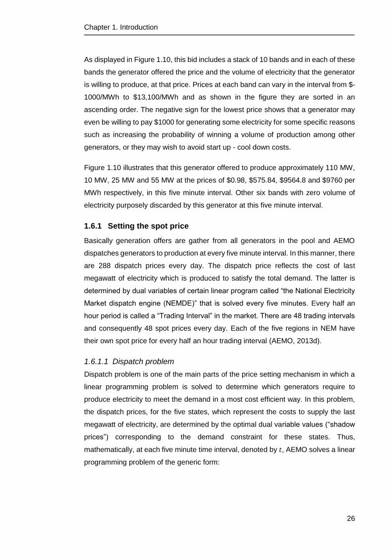
Figure 1.10 shows a generic bid stack structure by a typical South Australian
generator in a five minute interval. Basically, the structure of bids in Australian
electricity market has been designed in a way that allows generators to offer volume
and price of electricity production in a stack of 10 bands. As an example, the figure
below shows a bid offered by a generator in South Australia at a five minute interval
of 17:30 to 17:35pm on 31st March 2008.
Figure 1.10. Bid offered, March 31th 2008 at 17:30 (AEMO Website, accessed 2/8/2012).
6 The Reliability Panel was established by the AEMC under the National Electricity Law and
Rules. This panel regulates standards to ensure the power system remains secure and
reliable. (Source, AEMC website, Accessed 2/7/2014)
7 Australian Energy Market Commission.
0
20
40
60
80
100
120
140
-976 0.98 96.62 141.52 292.8 575.84 976 9174.4 9564.8 9760
Price
Volume (MWh)
Chapter 1. Introduction
26
As displayed in Figure 1.10, this bid includes a stack of 10 bands and in each of these
bands the generator offered the price and the volume of electricity that the generator
is willing to produce, at that price. Prices at each band can vary in the interval from $-
1000/MWh to $13,100/MWh and as shown in the figure they are sorted in an
ascending order. The negative sign for the lowest price shows that a generator may
even be willing to pay $1000 for generating some electricity for some specific reasons
such as increasing the probability of winning a volume of production among other
generators, or they may wish to avoid start up - cool down costs.
Figure 1.10 illustrates that this generator offered to produce approximately 110 MW,
10 MW, 25 MW and 55 MW at the prices of $0.98, $575.84, $9564.8 and $9760 per
MWh respectively, in this five minute interval. Other six bands with zero volume of
electricity purposely discarded by this generator at this five minute interval.
1.6.1 Setting the spot price
Basically generation offers are gather from all generators in the pool and AEMO
dispatches generators to production at every five minute interval. In this manner, there
are 288 dispatch prices every day. The dispatch price reflects the cost of last
megawatt of electricity which is produced to satisfy the total demand. The latter is
determined by dual variables of certain linear program called “the National Electricity
Market dispatch engine (NEMDE)” that is solved every five minutes. Every half an
hour period is called a “Trading Interval” in the market. There are 48 trading intervals
and consequently 48 spot prices every day. Each of the five regions in NEM have
their own spot price for every half an hour trading interval (AEMO, 2013d).
1.6.1.1 Dispatch problem
Dispatch problem is one of the main parts of the price setting mechanism in which a
linear programming problem is solved to determine which generators require to
produce electricity to meet the demand in a most cost efficient way. In this problem,
the dispatch prices, for the five states, which represent the costs to supply the last
megawatt of electricity, are determined by the optimal dual variable values (“shadow
prices”) corresponding to the demand constraint for these states. Thus,
mathematically, at each five minute time interval, denoted by 𝑡, AEMO solves a linear
programming problem of the generic form:

Chapter 1. Introduction
27
min 𝑐(𝑡)𝑇𝑥
𝐴𝑥 ≥ 𝑏(𝑡) (𝐿𝑃(𝑡))
𝑥 ≥ 0.
The input data needed to construct (𝐿𝑃(𝑡)) include generator’s bid stacks,
transmission network capacity and cost and many other parameters. The objective is
to minimize the cost involving energy cost, ancillary service cost, transmission
network cost and some security penalties to avoid overflow on the lines (Conticini,
2010).
Figure 1.11 shows NEM electricity grid which includes 5 interconnected regions.
In (𝐿𝑃(𝑡)), 𝑏(𝑡) includes demands in period t and there is a separate demand
constraint for each region and the dispatch prices are the optimal dual variables
y𝑗(𝑡), 𝑗 = 1,2, … ,5 corresponding to the five demand constraints.
Figure 1.11. NEM electricity grid.
1.6.1.2 Spot price
Thus for each five minute interval t, an optimal solution of (𝐿𝑃(𝑡)), determines five
dispatch prices y𝑗(𝑡)for the five states. In this way 288 dispatch prices are determined
every day, for each state. Next, AEMO switches to the coarser, thirty minute, trading
intervals denoted by . In each state, the spot price y𝑗() for the trading interval is
the average of six (five minute) dispatch prices in a half an hour trading interval,
namely

Chapter 1. Introduction
28
y𝑗() =1
6[y𝑗(𝑡1) + y𝑗(𝑡2) + ⋯ + y(𝑡6)]. (1.1)
The above is the price according to which all generators in the state j are going to be
paid equally no matter what price they have offered in their biding stacks.
Remark 1.1 It essential to emphasize that all generators selected to produce
electricity in the state 𝑗 during the trading interval will be paid at the spot price y()
per MW for every megawatt they produce during that trading interval, irrespective of
the prices comprising their original bid stacks.
1.6.2 Trends in the electricity spot price
As mentioned by AER (2012), during the years 2006-2010, most of the regions
experienced peak electricity price. Many factors contributed to the high volatility in
electricity price. For instance, drought was one of the reasons that limited the
production of hydro plants due to shortage of water which resulted in problems in
electricity production. Also as mentioned in AER (2013c) report evidence of exercising
market power by generators has been observed, specifically by AGL in South
Australia, which had a considerable effect on the price volatility between the years
2008-2010.
Since then, electricity demand has had a decreasing trend and with the aid of
renewable energy generation in the grid, the spot price had also a decreasing trend
until 2012. During the years 2012-13, the decreasing trend in the spot price changed
its direction again and the market experienced high spot prices. The average spot
prices increased to $70/MWh, $61/MWh, $74/MWh, $56/MWh, $49/MWh for the for
the regions of Queensland, Victoria, South Australia, New South Wales and Tasmania
in 2012-13. In general, the electricity price across NEM, by around $31/MWh (AER,
2013a).
One of the main reasons for the increasing spot price during 2012-13 was thought to
be the impact of carbon pricing scheme introduced on 1 July 2012 which sets $23 per
tonne of emission. However, the carbon price was not the only reason contributing to
raising the prices. As mentioned by AER (2013c), in the two states of Queensland
(August-October 2012) and South Australia (April-May 2013) which had the largest
increase in electricity prices, some opportunistic bidding behaviour by generators has
been noticed.

Chapter 1. Introduction
29
Indeed, the dependence of the spot price on the generators’ bids in the pool may be
one of the main reasons for electricity price fluctuations. Although this mechanism
was created to balance the demand and supply with the minimum possible cost,
research shows that there has been times of the year when some generators were
able to exercise their market power. There is a broad literature in this area ((Brennan
and Melanie (1998), Wolfram (1999) and etc.). This has contributed to the high
electricity price volatility in the Australian electricity market particularly in the recent
decade. The spot price could be highly volatile and in some trading intervals it even
has reached to the previous maximum cap price of $10000/MWh7F
8. In Chapter 2 more
literature in this area will be mentioned.
1.7 FINANCIAL RISK MANAGEMENT IN NEM
The fact that electricity price in the wholesale electricity market in Australia is
dependent on the generators bids contributes to the price volatility in some trading
intervals of the year. In addition, the limitation in the expansion of interconnectors in
Australia also made the transmission of electricity a difficult task. Therefore,
transmitting electricity can depend mostly on the local generations. Furthermore,
other factors such as seasonal effects on rising demand is also contributing to
fluctuation in the electricity price at specific times of the year. All these factors can
lead to variation in the financial risk in the wholesale electricity market. This led to
designing the appropriate financial contracts to hedge the risk of the electricity price
volatilities for the stakeholder.
The hedge contracts are generally set between generators and consumers. These
contracts reduce the risk of price volatility by locking the price in the financial contracts
and are independent of the rules in the market and do not mean to balance the supply
and demand. In hedge contracts, a strike price is set in these contracts for the
electricity traded on the spot market. This enables parties to exchange money based
on the agreed strike price for the specific amount of electricity.
Figure 1.12 shows an example of a hedge contract on the electricity in the financial
market. This contract is between seller of the contract and the buyer, and the strike
price is set to $40/MWh. As illustrated in the figure, when the spot price is lower than
$40/MWh, the buyers of the contract pays the seller, the difference between the
agreed strike price and spot price. In reverse, sellers are required to pay the difference
8 After July 2013 the price cap increased to $13,100/MWh

Chapter 1. Introduction
30
to buyers when the spot price goes beyond the strike price. Many appropriate hedge
contracts are designed in the financial market to deal with this volatility in the electricity
price. For instance, in Sydney Future Exchange, future and option electricity contracts
has been traded for the New South Wales electricity market (AEMO, 2010).
Figure 1.12. An electricity hedge contract (Source: AEMO July 2010).
1.8 THE RETAIL ELECTRICITY MARKET
The retailers in the electricity market are the parties which buy electricity from the pool
(wholesale electricity market) and sell to the customers 8F
9. The main role of retailer in
the wholesale electricity market is to buy electricity from the pool and with providing
the transportation services, sell it to the consumers. Table 1.3 shows a number of
retailers in Australia which supply electricity to the consumers in October 2013.
As Table 1.3 shows retails are not necessarily active in all the regions. Three privately
owned retailers of AGL, Origin Energy and Energy Australia are the major suppliers
in south and eastern parts of NEM. They cover about 77 percent of electricity supply
to the consumers in their regions at 30 June 2013 (AER, 2013a).
9 It should be mentioned that there are some consumers who directly buy electricity from the pool without the aid of retailers.
0
20
40
60
80
100
120
140
160
180
4:00 5:00 7:00 8:00 9:00 13:00 15:00 17:00 19:00 21:00 22:00 0:00
Spot
Price($
)
Time
Buyer pays seller differenecebetween agreed strike price andspot price
Seller pays buyerdifferenecebetween agreedstrike price andspot price
Strike price
Spotprice

Chapter 1. Introduction
31
Table 1.3. Energy retailers- small customer market, October 2013 (AER, 2013a).
Retailer Ownership QLD NSW VIC SA TAS ACT
ActewAGL Retail ACT government and AGL Energy
AGL Energy AGL Energy
Alinta Energy Alinta Energy
Aurora Energy Tasmanian Government
Australian Power and Gas
AGL Energy
BlueNRG Blue Energy
Click Energy Click energy
Diamond Energy Diamond Energy
Dodo Power and Gas
M2 Telecommunication Group
EnergyAustralia CLP Group
Ergon Energy Queensland Government
Lumo energy Infratil
Momentum Energy Hydro Tasmania (Tasmanian government)
Neighbourhood Energy
Alinta Energy
Origin Energy Origin Energy
People Energy People Energy
Powerdirect AGL Energy
Powershop Meridian Energy
Qenergy Qenergy
Red Energy Snowy Hydro
Sanctuary Energy Living Choice Australia/Sanctuary Life
Simply Energy International Power
1.8.1 Retail price
In general, the energy bills that consumers pay consist of various costs such as cost
of whole sale energy, transmission and distribution network costs and also retail cost.
Table 1.4 shows the share of these costs in each region in a typical electricity retail
bill for a residential consumer.
As shown in Table 1.4, the highest portion of electricity cost is related to the
transmission and distribution of electricity through network. Carbon costs are
introduced in July 2012. South Australia and Tasmania had the lowest percentage in
carbon price as they have significant renewable generation. Green costs are related
to schemes supporting renewable generation development, low emission generation
and also supporting energy efficiency (AER, 2013b).
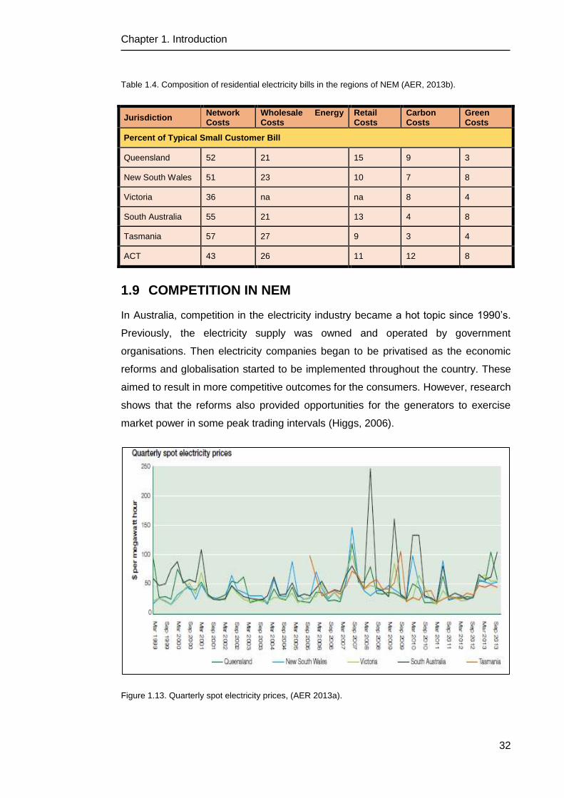
Chapter 1. Introduction
32
Table 1.4. Composition of residential electricity bills in the regions of NEM (AER, 2013b).
1.9 COMPETITION IN NEM
In Australia, competition in the electricity industry became a hot topic since 1990’s.
Previously, the electricity supply was owned and operated by government
organisations. Then electricity companies began to be privatised as the economic
reforms and globalisation started to be implemented throughout the country. These
aimed to result in more competitive outcomes for the consumers. However, research
shows that the reforms also provided opportunities for the generators to exercise
market power in some peak trading intervals (Higgs, 2006).
Figure 1.13. Quarterly spot electricity prices, (AER 2013a).
Jurisdiction Network Costs
Wholesale Energy Costs
Retail Costs
Carbon Costs
Green Costs
Percent of Typical Small Customer Bill
Queensland 52 21 15 9 3
New South Wales 51 23 10 7 8
Victoria 36 na na 8 4
South Australia 55 21 13 4 8
Tasmania 57 27 9 3 4
ACT 43 26 11 12 8

Chapter 1. Introduction
33
Figure 1.13 shows the quarterly base spot electricity price since deregulation. As
shown in Figure1.14, electricity spot price has experienced high fluctuations since
the deregulation in 1990s.
The volatility in the spot price was very high in the state of South Australia during the
years 2008-2010. AER (2013a) has directly mentioned that there exists evidence of
exercising market power in the recent years:
“In April 2013 the AEMC found potential for substantial market power to exist or be
exercised in future in NEM, particularly in South Australia. It recommended the
Standing Council on Energy and Resources (SCER) consider conferring on the AER
powers to monitor the market for that possibility. In May 2013 the SCER agreed to
task officials with further work around the need for changes to the National Electricity
Law before the SCER considers its policy position” (AER, 2013a, p33).
It should be mentioned that, Australia is not the only country that has experienced
exercising market power in the restructured electricity market. There is some evidence
that such phenomena have also occurred in other countries such as USA and UK.
This issue will be discussed further in Chapter 2.

34
2. CHAPTER 2. PRICE VOLATILITY
AND MARKET POWER IN
ELECTRICITY MARKET
To encourage the competitiveness among producers the reforms in the electricity
market designed in many countries around the world such as Australia. Although, the
primary aim of the deregulation was to encourage market competition and to eliminate
monopolistic market power, there is evidence that market power has been exercised
within generation business in the electricity markets. There are various published
papers that address price volatility and possible market power abuses all around the
world.
Borenstein et al. (2000) addressed the potential for market power in California’s
wholesale electricity market after deregulation. Joskow and Kahn (2002) also
provided evidence of generators exercising market power which was a result of
withholding capacity offered to the market in California during 2000 and 2001.
David and Wen (2001) brought evidence of the market power in the electricity supply
markets during the late 1990s. They highlight the fact that, despite accepting the
deregulation in electricity markets, some generators are still able to exercise market
power in peak period of demand. Mount (1999) also focuses on high price rises in UK
electricity market as a result of two leading generators exercising market power in the
1990s.

Chapter 2. Price Volatility and Market Power in Electricity Market
35
Brennan and Melanie (1998) examined the potential market power by strategic pricing
behaviour by generators in Australian electricity market. They provided evidence of
non-competitive bidding behaviour by some large generators mainly in the high
demand periods. Hu et al (2005) believe that large generators had the ability to push
the price higher by withholding their generation capacity in the Australian National
Electricity Market. There also have been other shifts in electricity prices in the
restructured electricity markets examined by Wolak (2000) and Mount (1999).
Most definitions of market power emphasise the fact that the exercise of market power
needs to be profitable. However, further investigations need to be carried out to
analyse whether this profitability occurred intentionally or by accident. In other words,
high prices are not necessarily an indication of generators exercising market power,
rather they can be a result of a shortage of supply in a competitive market. Therefore,
further investigation needs to be done to examine the actual exercise of market power
in the electricity markets.
Besides it should be mentioned that, exercising market power may not be the only
reason for the price volatility in the electricity markets. Recall that, electricity has a
specific characteristics which need to be considered while assessing the
competitiveness among generators in the market. These characteristics include, high
volatility in the electricity demand during the day, the lack of flexibility to response to
the sudden increase in the electricity demand, difficulty in electricity storage and the
essential need to balance the electricity demand and supply instantaneously through
time. These features contributed to the cost of electricity production being highly
volatile even within a short period of time such as a day (ABARE 2002).
As understanding of the volatility process is critically important to distributors,
generators and market regulators allowing them to better manage their financial risk,
in this chapter we aim to examine some mechanisms by which generators could
exercise market power9F
10. Section 2.1 describes techniques which were used by
economists to identify the possibility of exercising market power by generators.
Moreover, the history of price volatility in Australia and also discussion of exercising
of market power by generators in the literature are provided in Section 2.1 and 2.2.
We focus on the state of South Australia which had the highest spot price fluctuations
since the deregulation was introduced.
10 It is important to note that it is not within the scope of this thesis to determine whether or not Australian generators have exercised market power but only to demonstrate that such possibilities exist in the market.

Chapter 2. Price Volatility and Market Power in Electricity Market
36
2.1 INDICES AND MODELS OF DETECTING MARKET POWER
Market power is defined as the ability to change the price from the competitive levels.
There have been number of measures and tools identified by economist to detect the
exercise of market power in different industries. Apparently, some of these measures
would be suitable for specific industries and some may not be suitable to be used in
the electricity market (Stoft, 2002).
Generally, the detection of market power includes two forms of “Potential” for market
power or actual “Exercise” of market power. Monitoring the potential for exercising
market power is as important as detecting the actual exercise of market power for
market monitors as it is considered as a useful procedure for prevention of any
exercise of market power (Twomey, P. et al, 2005).
Detecting market power in electricity markets is not easy (Baker, J., 1992, Twomey,
P. et al, 2005 and Blumsack, 2003). On the other hand, electricity market has some
characteristics which facilitate the detection of the market power. For instance, it is
possible to estimate the cost of production more precisely in electricity market than in
many other industries.
Various measures are available to detect potential for market power and actual
exercise of market power by generators. Here we briefly provide an introduction to
some of these measure which have been used to monitor the market power in
industries such as electricity market.
2.1.1 Market power indices
Traditional industrial organisation theory defines some industrial indices which have
been also applied in the electricity markets to measure the potential for exercising
market power. In this section some of these measures and their application are
outlined.
2.1.1.1 Market share
The motivation behind this index is that the more concentrated a market, the more
likely is the ability of its participants to exercise market power. The market share
concentration ratio is the percentage of market share of 𝑛 largest companies in the
industry.
In order to calculate this index many features need to me be measured first such as
identifying the product in the market and the competitors in the market. Also a
“significant market share” threshold needs to be defined in a way that any market

Chapter 2. Price Volatility and Market Power in Electricity Market
37
share above this threshold would be considered as a sign of potential for market
power (Twomey, P. et al, 2005).
Basically, market share provides information about the ratio of the capacity which is
controlled by one or number of generators. In the electricity market with this
specification, the exercising of market power by generators is more likely. As an
example, Australian Energy Regulator indicates the relatively strong market positions
held by AGL Energy in South Australia, Macquarie Generation in New South Wales,
and the state-owned generators CS Energy and Stanwell in Queensland in the recent
years (AER, 2013a).
2.1.1.2 Herfindahl-Hirschman Index (HHI)
The Herfindahl-Hirschman Index (HHI) determines the size of the firm as the sum of
squared of percentages of market shares of all firms in the market.
𝐻𝐻𝐼 = 𝑆12 + 𝑆2
2 + ⋯ + 𝑆𝑛2,
where 𝑆𝑖2 is the percentage market share of company 𝑖. The benefit of using 𝐻𝐻𝐼 is
that it also considers the size of other participants in the market. Obviously, a
company with market share of 20% where other competitors have small percentage
of share has a different market power compared to the situation where that company
is the second or third largest player in a highly concentrated market. (Calkins, 1983)
Figure 2.1 HHI in NEM during 2008-09 to 2012-13 (AER, 2013a).
When a market includes a large number of firms, 𝐻𝐻𝐼 can even approach zero but in
a monopoly situation it reaches (100%)2 or 10,000. High value of 𝐻𝐻𝐼 shows a less
competitive situation in the market. Figure 2.1 shows the 𝐻𝐻𝐼 in NEM regions from
2008 to 2013. As shown in Figure 2.1 the state of SA had the highest 𝐻𝐻𝐼 during
2008-2009.

Chapter 2. Price Volatility and Market Power in Electricity Market
38
2.1.1.3 Pivotal Supplier Indicator (PSI)
Pivotal supplier index considers not only the supply but also the demand conditions
in the market to measure the potential for market power. It measures whether a certain
generator has a crucial (or pivotal) role in meeting demand.
Basically the generator is called pivotal if the capacity of that generator is greater than
the “surplus supply”10F
11. Pivotal supplier indicator is defined as a binary indicator which
is set to one or zero where the generator (supplier) is pivotal or not pivotal at point in
a time, respectively. It is called Pivotal supplier index which helps to determine the
percentage of time when a supplier was pivotal. Bushnell et al (1999) found that the
largest supplier in the region of Wisconsin/Upper Michigan was a pivotal supplier for
55% of the hours in a year.
AER (2013a, pp.51-57) lists the percentages of time when the largest generator in the
market became pivotal in 2012-13 across NEM regions in Table 2.1. As shown in
Table 2.1, state of South Australia has the highest potential to exercise market power
during 2012-13.
Table 2.1. Percentage of trading intervals when large generators were pivotal in 2012-13
QLD NSW VIC SA
17 18 20 29
2.1.1.4 Residual Supply Index (RSI)
The Pivotal supplier Index mentioned above, has been criticised specially on the
implementation of this index. These criticism include the application of this index to
address exercise of market power just for peak hours, the lack of coordination among
generators and etc (see Vassilopolous 2003). Therefore, the Residual Supply Index
developed to address these criticism which is similar to PSI but it is not measured by
the binary basis rather a continuous scale.
The Residual Supply Index (RSI) measures the extent to which one or more generator
can be “Pivotal” in the market. A generator 𝑔 is called pivotal in a trading interval if
demand in that trading interval exceeds the capacity of all other generators in the
market. Note that this notion of “pivotal” need not be the same as that described in
section 2.1.1.3. It measures the supply capacity remaining in the market after
subtracting company 𝑔’s capacity of supply.
11 The surplus supply is the difference between total supply and demand.

Chapter 2. Price Volatility and Market Power in Electricity Market
39
𝑅𝑆𝐼𝑔 =𝑇𝑜𝑡𝑎𝑙 𝐶𝑎𝑝𝑎𝑐𝑖𝑡𝑦 − 𝐶𝑜𝑚𝑝𝑎𝑛𝑦 𝑔′𝑠 𝑅𝑒𝑙𝑒𝑣𝑎𝑛𝑡 𝐶𝑎𝑝𝑎𝑐𝑖𝑡𝑦
𝑇𝑜𝑡𝑎𝑙 𝐷𝑒𝑚𝑎𝑛𝑑,
where, total capacity includes both regional supply and also supply imports. Relevant
capacity for a company 𝑔 shows the company’s capacity minus all the contract
obligations of that company. Value of 𝑅𝑆𝐼𝑔 shows how company 𝑔 has influence on
the market to meet the demand. An 𝑅𝑆𝐼𝑔 value less than a 100 percent shows that
the company is a pivotal player in the market. Sheffrin (2002) believes that RSI must
be more that 110 percent for 95 percent of the hours in a year.
Figure 2.2. RSI-1 index at times of peak demand, AER (2013a).
AER provides evidence of potential market power by largest generator in the state of
SA during 2008 using RSI-1. This index measures the ratio of demand that can be
met by all but the largest generator in a region. If RSI-1 is less than 100 percent then
the largest generator becomes pivotal and indicates a less competitive market.
Figure 2.2 shows the RSI-1 index at times of peak demand since 2008 in NEM. As
shown in Figure 2.2 SA had the highest potential to exercise the market power by the
largest generator. In South Australia, AGL is the largest generator and offers around
34 percent of the total capacity in the state11F
12.
According to AER (2013a), since 2012 some of thermal generators as Alinta has
decided to withdraw capacity from market. As it is reflected in Figure 2.2, this
12 International Power with 21 percent of the total capacity, Alinta with 12 percent and Origin
Energy with 12 percent are other large firms is South Australia.

Chapter 2. Price Volatility and Market Power in Electricity Market
40
increased the pivotality of AGL, as the largest generators in South Australia, to meet
demand during peak trading intervals.
2.1.1.5 Residual demand analysis
To find the residual demand curve corresponding to a company 𝑔 , one should
subtract all of supply offers by the other participants in the market from the demand
curve. The elasticity12F
13 of this curve is an indicator of company 𝑔’s incentive to exercise
the market power. In a competitive market, a company has no power to raise the price
by capacity withholding and has a very high elastic residual demand curve. High
elasticity shows that, this company has the power to not to be disadvantaged by
charging high prices (Baker & Bresnahan, 1992). As an example, Wolak (2003) shows
the incentive for five large electricity supplier to exercise the market power in
California 1998-2000.
2.1.2 Behavioural indices
The other indicators to measure the competitiveness in the market are behavioural
indicators. These indicators examine the relationship between generators bidding
behaviour and the spot price outcomes. The following are some of the main
behavioural indices defined by economists.
2.1.2.1 Bid-Cost margins
Comparing company’s bid prices and marginal cost would also be an indication of
exercising market power. In a competitive market, it is expected that generators bid
at a level close to their marginal cost. If a company frequently bids at much higher
prices than the marginal cost, then this may be an indication of exercising market
power by that company. The following indices, Lerner Index and Price-Cost Margin
Index, measure whether the market power exists. In this sense:
𝐿𝐼 = (𝑃 − 𝑀𝐶)/𝑃,
𝑃𝐶𝑀𝐼 = (𝑃 − 𝑀𝐶)/𝑀𝐶,
where 𝑃 and 𝑀𝐶 show the price and marginal cost respectively. In a perfectly
competitive market, the value of these indices would be zero. However, estimating
the marginal cost of a company is not always an easy task which is one of the main
difficulties in determining the accurate value of these indices. There is some evidence
13 Elasticity is a measure used in economics to show the sensitivity of the change in quantity demanded of a good or service to a change in its price, ceteris paribus ( More information available at Samuelson, 2001).

Chapter 2. Price Volatility and Market Power in Electricity Market
41
of companies exercising market power in California 2000-2001, as well as in England
and Wales in 1990-1991 (Twomey, P. et al, 2005).
2.1.2.2 Withholding analysis
Withholding analysis is the basic measure to detect any withholding capacity in the
electricity market. Two types of withholding are examined in this measure: economic
withholding and physical withholding. Economic withholding refers to the situation
where output is bid by generators at over the competitive bid price. In physical
withholding the output is not bid to the market at all. Both of these capacity
withholdings would reduce the supply in the market (Twomey, P. et al, 2005). Table
2.2 shows the average capacity withheld by large generators in NEM during 2008-
2010 and 2011-2013 periods when the spot price rose above $300 per MWh13F
14.
Table 2.2. Average capacity not dispatched when spot price exceeds $300/𝑀𝑊ℎ, AER (2013a).
Generator
Capacity Not Dispatched (MWh)
July 2008-December 2010 January 2011- June 2013
CS Energy (QLD) 543 826
Macquarie Generation (NSW)
243 41
International Power (VIC) 260 177
AGL Energy (SA) 328 250
Figure 2.3 also shows the relationship between capacity withholding and price rise
during 2008-2013 in South Australia. As shown in the Figure 2.3 AGL which is the
largest generator in SA and offers around 34% of the total capacity, tends to withhold
part of its capacity when the price is relatively low.
For example, as shown by the dark green line, the spot price was in the range of $0-
$25 in years 2008-09. AGL offered only some 30% of its total capacity to the market.
The fact that for three, out of five, of these curves the slope is negative for higher
values of spot price should be noted, as it raises questions as to why capacity was
withheld at times of increasing spot price.
14 This price is sufficient to cover the marginal cost of majority of plants in NEM (AER 2013a).

Chapter 2. Price Volatility and Market Power in Electricity Market
42
Figure 2.3. Average annual capacity utilisation, AGL Energy, South Australia, AER (2013a).
2.1.3 Other indices
2.1.3.1 Simulation models
In this form of market power analysis, some aspects of market are simulated with
sophisticated modelling techniques to make a benchmark for the comparison of the
market outcomes if the generators behaved differently. The two popular models in
this area are as follows.
(i) Competitive benchmark analysis
In this form of analysis a hypothetical competitive market is simulated. This provides
a benchmark to compare the actual price with a hypothetical price if all generators
behaved differently. For this purpose, the generation technologies data are collected
to estimate the supply curve which ultimately will result in estimating the marginal cost
of production. However achieving this goal is not an easy task and determining a
proper comparative benchmark has been always a controversial task (Twomey, P. et
al, 2005).
(ii) Oligopoly simulation models
Oligopoly simulation models provide a game theoretic framework to estimate the
market price within a specified market design and structure. These models are more
powerful than any other indices as they consider many factors to examine the exercise
of market power. These factors include, demand elasticity, supply curve,
concentration, forward contracting and transmission constraints. One of the most
powerful models in this area is Cournot competition model which identifies the market
equilibrium based on the generators level of output (Twomey, P. et al, 2005).

Chapter 2. Price Volatility and Market Power in Electricity Market
43
2.1.3.2 Net revenue benchmark analysis
Net revenue benchmark is another measure to analyse the existence of market
power. Although high net revenue is not necessarily an indication of market power,
many researchers consider abnormal profits as a useful measure for monitoring
market power in electricity markets (Twomey, P. et al, 2005).
2.2 PRICE VOLATILITY IN THE AUSTRALIAN ELECTRICITY MARKET
The current Australian Electricity Market was designed to operate in a competitive
national market using private industry. However, evidence shows that the volatility in
the electricity spot price has been one of the electricity market features since the
deregulation (Quiggin 2001). The main reasons which can lead to price volatility
recorded in the literature are:
(i) When a generation station falls over and its capacity will be removed from the
pool.
(ii) Extreme temperature conditions which directly affects the demand. For
instance, in the cold winter days or hot summer days the consumption of air-
conditioning rises and increases the load significantly. In this situation
generally generators bid at higher price levels as they claim they need to
generate more to meet the demand.
(iii) Any fault in the network may increase the prices as sections of the grid may
be unable to work properly (IEA, 2001).
Basically, considerable fluctuations in the electricity price in the Australian electricity
market occurred during the years 2008-2010 when the electricity price reached to the
maximum of $10,000/MWh for a number of trading intervals. During 2009-10, there
were 95 trading intervals which had a corresponding spot price greater than
$5000/MWh in the market. Thereafter, as a result of some changes in the market
conditions, the number of extreme electricity spot price declined. The reduction in
energy use by consumers was one of the main reasons as it caused surplus in the
installed capacity in the most of the regions.
Although the number of price spikes has decreased since 2010, there has been more
trading intervals with the corresponding spot price greater than $200/MWh. In 2012-
13, there were 704 such trading intervals compared to only 99 in the year 2011-12.
This has happened mainly in the states of Queensland and South Australia. Moreover,
during summer 2013, Queensland experienced 116 instances of prices above
$300/MWh and 16 spot prices above $1000/MWh. One of the main reasons was the

Chapter 2. Price Volatility and Market Power in Electricity Market
44
12 percent lower capacity offered by the generators during summer time comparing
to the same quarter in 2012 (AER, 2013a).
Disorderly bidding by generators was thought to be one of the underlying reasons
including the price spikes. Such disorderly bidding is not limited to the central
Queensland. Other regions in NEM have experienced these forms of behaviour by
generators. “Disorderly Bidding” has been defined by AER (2013b) as a bidding
strategy which is in contrary to the underlying cost structure and/or technical
limitations of generation plant.
“ In particular, generators tried to maintain output levels and receive high spot prices
by rebidding capacity from high to low (or negative) prices.” (AER, 2013b, p.40).
Table 2.3 shows the average of spot prices since the deregulation in the 4 regions of
NEM. As highlighted with the arrows in Table 2.3, the average of spot price seem to
experience significant increase in specific years. For instance, the average of spot
price increase from around $30/MWh to more than $50/Mwh from the year 2005-06
to 2006-07 in all of the 4 regions. This significant increase in the average of spot price
also occurred from 2011-12 and lasted to 2013-14 in these regions of NEM.
Table 2.3. Average of spot prices per year, (AEMO accessed 23.09.2014).
Year NSW QLD SA VIC
1999-2000 28.27 44.11 59.27 26.35
2000-2001 37.69 41.33 56.39 44.57
2001-2002 34.76 35.34 31.61 30.97
2002-2003 32.91 37.79 30.11 27.56
2003-2004 32.37 28.18 34.86 25.38
2004-2005 39.33 28.96 36.07 27.62
2005-2006 37.24 28.12 37.76 32.47
2006-2007 58.72 52.14 51.61 54.8
2007-2008 41.66 52.34 73.5 46.79
2008-2009 38.85 34 50.98 41.82
2009-2010 44.19 33.3 55.31 36.28
2010-2011 36.74 30.97 32.58 27.09
2011-2012 29.67 29.07 30.28 27.28
2012-2013 55.1 67.02 69.75 57.44
2013-2014 52.26 58.42 61.71 51.49
2014-2015 39.88 31.63 46.42 37.39

Chapter 2. Price Volatility and Market Power in Electricity Market
45
The rise in the average of spot price is even more substantial in South Australia. As
shown in Table 2.3, the increase in the average of spot price in South Australia started
from 2005-06 where it increased from about $37/MWh to about $51/MWh in 2006-07.
This increasing trend continued to the year 2009-10. Between these years the
average of spot price per year even reached to a considerable high price of $73/MWh
in 2007-08.
Furthermore, similar increasing trend occurred during the years 2011-12 to 2013-14
in South Australia. As mentioned by AER (2013b, P38), the significant increase in the
average of spot prices was often unrelated to the demand. In South Australia, even
minor increases in the demand led to spikes in the electricity price as a result of
significant decrease in the capacity offered by generators. Section 2.2.1 provides
more detail about the history of price volatility in South Australia.
2.2.1 Spot price volatility in South Australia
Since the deregulation in 1990’s, exercising market power has been reported in some
periods of time in various regions of NEM. As mentioned above, one of the states
which had experienced high electricity price volatility particularly in the higher demand
periods is South Australia. For this reason, in this thesis, our focus is mainly on the
variation in the spot prices and its underlying causes, in South Australia.
Figure 2.4. Electricity demand and spot price at January 2010.
During the years 2008-2010, South Australia has also experienced price spikes in
high demand periods similar to the other regions of NEM. The supply-demand
condition is often claimed to be the tightest in South Australia since the blackout in
summer 2009. Figure 2.4 shows the spot price and demand at half hour intervals for
all 1488 trading intervals within the month of January 2010 in the state of South
Australia.
Jan 8th, 4pm
0
1000
2000
3000
4000
5000
6000
7000
8000
9000
10000
0
1000
2000
3000
4000
5000
6000
7000
8000
9000
10000
Dem
an
d (
MW
)
Sp
ot
Pri
ce (
$/M
Wh
)
Trading Interval

Chapter 2. Price Volatility and Market Power in Electricity Market
46
As Figure 2.4 illustrates, spot prices which are shown by the red curve exhibit higher
fluctuations than demand which is depicted by the blue curve. As seen in the figure,
most of the time spot price varies over a range of $100 per MWh but it also
approaches the very high price of $10,000 in some trading intervals. For instance, the
spot price for the interval of January 8th at 4:00pm reached to almost $10,00014F
15 for
the state of SA. This happened even though the demand did not have an exceptionally
high increase during that period.
Furthermore, South Australia experienced high price volatility especially in April-June
2013. The lack of generation capacity was the main reason resulting in these
fluctuations. The reduction in the generation capacity offered was mainly done by
three major generators, “Alinta”, “International Power” and “AGL Energy”. Alinta
offlined both Northern power station units and International Power reduced the
capacity offered by Pelican Point power station to the half of the maximum available.
AGL energy offered around 225MW less capacity at Torrens Island and also offered
higher prices for the remaining capacity (AER, 2013a).
In general, the generators in South Australia offered 700MW lower capacity during
April-June 2013 compared to the same period in 2012. This led to 212 spot prices
above $200/MWh, which included 19 spot prices above $1500/MWh. It should be
mentioned that, during the corresponding period in 2012, there were no trading
intervals with spot prices above $200/MWh. The average of spot price in April-June
2013 was about $106/MWh which was almost twice that of other regions in NEM.
While high spot price in South Australia during April-June 2013 led to import electricity
from Victoria, the lack of available capacity was the key factor which led to the tight
condition to meet the demand (AER, 2013a).
Table 2.4 provides more information about the history of price volatility in South
Australia. As Table 2.4 illustrates besides the significant increase in the electricity
prices, disorderly bidding by generators led to negative prices in some trading
intervals15F
16. Table 2.4 also illustrates that during the years 2008-2010 there were 59,
77 and 44 trading intervals, respectively, which had the corresponding spot price
reaching to above $1000/MWh16F
17. Also the average of spot price reached its peak
during these years. It should be mentioned that, during 2007 to 2011, the increase in
15 It should be mentioned that, $10,000 was the market price cap before 30 June 2010 and that it was increased to $12,500 per MWh thereafter. 16 More information is available in AER (2013b), State of the energy market 2012, pp.16-17 and 46-47. 17 In Chapter 3 the categories of spot price will be introduced. Based on the categories of spot prices we call these trading intervals as “High” spot price periods.

Chapter 2. Price Volatility and Market Power in Electricity Market
47
the average annual spot price in South Australia was more than 50% higher compared
to the other regions of NEM (AEMO, 2010).
Table 2.4. History of price spikes in South Australia.
Year 2006 2007 2008 2009 2010 2011 2012 2013
Number of trading interval with the corresponding spot price greater than $1000/MWh
33 21 59 77 44 22 13 75
Price
Min -160.37 -888.78 -1000.00 -663.17 -996.70 -996.70 -995.70 -289.43
Max 7758.08 7813.10 9999.72 9999.92 9999.92 12199.53 4140.15 10627.00
Mean 38.68 57.50 66.38 60.47 40.28 37.41 44.21 71.68
Variance 17046.96 15033.01 272637.96 253996.36 114977.87 76116.29 5393.01 27712.24
𝐶𝑣 3.38 2.13 7.87 8.33 8.42 7.38 1.66 2.32
Demand
Min 767.54 784.15 847.36 834.21 814.70 853.99 868.62 728.59
Max 2873.03 2854.13 3079.82 3331.12 3120.89 3385.42 2939.39 2991.27
Mean 1494.98 1524.12 1527.40 1538.42 1547.25 1494.64 1477.40 1426.57
Variance 85509.34 102893.12 101064.42 125910.03 106537.83 86109.79 83056.06 91027.32
𝐶𝑣 0.20 0.21 0.21 0.23 0.21 0.20 0.20 0.21
Additionally, the variance of spot price demonstrates the high fluctuation in the
electricity price that the market experienced in these years. To measure the dispersion
of demand-price distribution in these years “Coefficient of Variation”,𝐶𝑣 of the spot
price, is reported in the seventh row of Table 2.4.
𝐶𝑣 =𝜎
𝜇
Comparing these measures in the spot price rows and the corresponding ones in the
demand rows in Table 2.4 indicates that the variation in the spot price was significantly
higher than the variation in the demand, specifically, during the years 2008-2010. We
provide more information to support the latter in Chapter 3.
This highlights the fact that the increase in electricity demand did not seem to be the
main underlying reason for the significant rise in the spot price during these years.
Instead, it seems that the price spikes in the electricity price during this period are
more related to the exercise of market power by generators than the shortage in the
generation capacity.
Energy Users Association of Australia has published a report in November 2012 which
directly addressed some concerns about possible exercise of market power by
generators during the years 2008-2011.

Chapter 2. Price Volatility and Market Power in Electricity Market
48
The high spot prices mainly happened during January-February when the
temperatures peaked. During that period, evidence of generators exercising market
power has been observed in the high demand periods where generators tried to
influence the spot price output by either strategic form of bidding behaviour or
withholding the generation capacity in high demand periods in recent years
(Mountain, 2012).
In a competitive market, if the prices are higher than the production costs, generators
should have enough incentive to increase their capacity to benefit the market
situation. However, there are indications that in some trading intervals in high demand
periods, generators tried to either withhold their generation capacity available to the
market or offer it in very high price bands. In 2008, a generation capacity of around
667 MW at Torrens Island Power Station was not available to the market in some
trading intervals. Same behaviour was seen by other generators in 2009-11 which
made the spot price reach the market price cap of $10,000/MWh at the time (CME,
2012).
It should be mentioned that, withholding capacity was not the only reason to shift the
prices to the peak levels. It has been observed that, there has been sufficient
generation capacity even during high demand periods. Further, in Chapter 3 we
examine forms of strategic bidding by generators and the corresponding risk imposed
on the end users by high spot prices.
2.2.1.1 Impact of exercise of market power on consumers
Generally, the degree of impact of spot price spikes on consumers depends on the
types of consumers in the market. For non-household consumers, these effects are
depending on other hedge contracts in the financial market and for household
consumers they depend on the standing contracts 17F
18 with AGL which are determined
by the Electricity Supply Commission of South Australia. Nonetheless, indirectly,
increases in spot prices will, ultimately, be passed on to consumers.
The price of hedge contracts in the financial market is also showing the same trend
as spot price over the period of 2007-11 in South Australia. Overall, higher spot prices
have resulted in higher future contracts prices and in this way generators have
18 The standing contract is the retail electricity contract that AGL SA must offer to all South Australian
small customers which is set by Electricity Supply Commission of South Australia. (ESCOSA, http://www.escosa.sa.gov.au/projects/177/1-july-2012-electricity-standing-contract-price-adjustment.aspx Accessed 23.08.2014).

Chapter 2. Price Volatility and Market Power in Electricity Market
49
benefited over the period of 2008-11 even when the spot prices reached the market
price cap of $10,000/MWh (AER, 2013a).
For household consumers in South Australia, the Essential Services Commission of
South Australia calculates the market price cap that AGL can charge residential or
small consumers. However, AEMC report has shown that this price is higher in South
Australia comparing to other regions of NEM (AEMC, 2011).
Overall, the significant increase in the number of price spikes in South Australia during
the year 2008-11 did not happen in other regions of NEM. This raises the questions:
(i) Does the very high Market Price Cap in NEM, recently increased to
$13,100/MWh, provides an incentive for generators to exercise market
power?
(ii) Is the flexibility of generators to shift the volume of generation offered to
different price bands as quickly as in five minute intervals, providing them
an opportunity to exercise the market power?
(iii) Does the market needs any change in the system design in Market Price
Cap or mandatory minimum volume to be offered at each price bands to
address the market power concerns?
2.3 STRUCTURAL VOLATILITY
As discussed above, volatility in the spot price for electricity is very high. Furthermore,
there are many factors that may be contributing to this high volatility. These range
from stochasticity of demands and weather conditions, through supply of renewable
energy (e.g., wind, solar), to financial management strategies such as hedging.
However, in this thesis we examine in some detail the impact of generators’ bidding
strategies on the volatility of spot prices, in the context of the mechanism by which
these prices are derived (see Section 1.6). We refer to this form of volatility as
“structural volatility” because it stems from the design of NEM and its regulations.
We feel that structural volatility deserves close scrutiny because the latter design is,
in principle, controllable and hence may be altered if changes were deemed to be
desirable. By contrast, volatility due to natural phenomena such as heat waves, or
cold spells cannot be significantly altered. Of course, the latter can still be understood
and its impact mitigated typically with the help of accurate forecasts, but this is not an
objective of the present study.

Chapter 2. Price Volatility and Market Power in Electricity Market
50
2.4 ALLEVIATING MARKET POWER
Some economists believe that as a result of special characteristics of electricity
markets, these markets are susceptible to the exercise of market power (Baker, J.,
1992, Twomey, P. et al, 2005 and Blumsack., 2003). First, as electricity is not easily
storable, the production is needed to match the demand instantaneously and this
makes the electricity supply to be relatively inelastic. Second, most of the electricity
consumers are not exposed to real time prices. Therefore, only the demand from very
large consumers is elastic to the real time prices. The inelasticity of electricity supply
and demand provides an opportunity for generators to exercise their market power
specifically in the high demand periods.
To alleviate the market power by generators, economists suggest a number of
solutions. These solutions include, “Structural solutions”, “Regulatory solutions” and
“Market rules solutions”. Structural solutions include encouraging the dominant
generators to divest their assets. At the same time, new competitors need to be
encouraged to enter the market by reducing or removing barriers to entry.
Regulatory solutions include imposing constraints to control the price such as market
price cap. Another regulatory solution would be setting the rule by which the dominant
generators are required to provide a certain amount of capacity to the network in the
long term.
Market rules solutions are the regulations which might be considered harsher such as
setting caps on unit specific bidding or asking for a specific information from
generators which would be very difficult to acquire (Twomey, P. et al, 2005).

Chapter 3. Statistical Approach
51
3. CHAPTER 3. STATISTICAL
APPROACH
As mentioned in Chapter 1, the wholesale electricity market is managed through a
spot market which consists of a pool where electricity supply and demand are
matched instantaneously. In this market, generators’ offers for electricity production
are designed to be submitted to the pool in a stack of 10 bands at every five minute
interval. This bid stack includes the volume and price of electricity they are willing to
generate and it needs to satisfy certain regulatory restrictions for floor and cap price
at each band. As mentioned by AEMO (2010a), the price offered at each band should
not be less than $-1000 and not more than $13,100 per MWh, respectively18F
19.
Combination of all these offers by generators determine, albeit indirectly, the marginal
price of generation and consequently the electricity spot price at each half an hour
interval. Recall that, AEMO collects all the bids offered by generators, then solves an
LP problem (Chapter 1, Section 1.6), which determines the generators who are
required to produce at each five minute interval, considering two main objectives of
meeting prevailing demand and minimising cost of production. The result of this
dispatch process is called a “Dispatch Price”. Thereafter, the spot price is determined
as the average of six dispatch prices in every half an hour trading interval (see
equation (1.1.)). This is the price that generators receive for the amount of electricity
they contributed and also the price that, ultimately, consumers need to cover.
19 Recall that this upper bound was increased from $10,000/MWh in 2010.

Chapter 3. Statistical Approach
52
In subsequent sections we investigate the effects of the different bidding behaviours
on both generators and end users as the two main constituencies in this market. We
aim to highlight the fact that the bid stacks offered by generators may increase the
income to generators and eventually impose the risk of higher cost to the end users
in the Australian electricity market 19F
20.
In Section 3.1 we differentiate the trading intervals using a spot price frame with two
different colours: high and low. Then we discuss the correlation of demands and spot
prices during selected periods of time in South Australia.
Section 3.2 is dedicated to introducing forms of strategic bidding behaviour by
generators. Further in Sections 3.3 - 3.4 we investigate how generators form specific
groups/clusters in which they follow the same pattern in changing the bid stack offered
to the pool, especially in the higher spot price trading intervals. In Section 3.5 we
examine the strength of the competition among generators and investigate whether
the electricity auction is running strong or weak in different trading intervals. Results
show that in the high spot price trading intervals the competition among generators
was weak and hence such auction underperformed.
In Section 3.6 we show that the competition among generators can be considered as
a lottery model. Then the choice of offering price and volume of electricity production
would be a tool for designing this lottery at each trading interval.
In Section 3.7 we examine the bid to cover ratio in the Australian electricity market.
We compute this ratio by the value of money claimed from the electricity pool by
generators divided by the value paid to the generators by AEMO.
Section 3.8 discusses the risk of loss to end users as an outcome of the lottery
designed by generators using risk measures such as Value at Risk and Conditional
Value at risk of loss.
3.1 CORRELATION OF ELECTRICITY DEMAND AND PRICE
This section discusses the correlation of demands and spot prices during selected
periods of time in South Australia. For simplicity, a spot price frame has been
designed using two different colours. Colours “Green” and “Red” are dedicated to the
trading intervals of “low” and “high” spot price periods and they are recognized using
20 Results of this chapter are published in a paper entitled ‘Australian Electricity Market and Price Volatility’ that appeared in the Annals of Operations Research (see Boland, J., et al (2011)).

Chapter 3. Statistical Approach
53
the two chosen ranges of $-1,000/MWh to $1,000/MWh and $1000 to $13,100. From
now on, we call these categories as Low, “L”, and High, “H”, spot price periods
respectively. Table 3.1 shows these categories of trading intervals by range of spot
price and the corresponding colour20F
21.
Table 3.1. Trading interval categories based on the level of sot price.
Low Spot Price Trading Interval $-1000/MWh < Spot Price < $1000/MWh
High Spot Price Trading Interval $1000/MWh < Spot Price < $12500/MWh
Based on the this trading interval categories, each point in Figure 3.1 shows the
correlation of demand and price in the two mentioned categories of spot price periods.
It should be mentioned that each point in this figure, corresponds to the correlation of
electricity price and demand in a day, using 48 trading interval data points available
in that certain day.
The colours are assigned based on the category of highest spot price occurring in that
specific day. For instance, as there exist at least one trading interval in the day of Jan
8th when the spot price exceeded $1000 per MWh we show the whole day of Jan 8th
by a red colour. By assigning a red or green colour we do not necessarily mean that
the spot prices corresponding to all trading intervals of the day are in the categories
of H and L (Table 3.1). These colours show that within the days with say red colour,
there exists at least one trading interval in which spot price was in the interval (1000,
13100).
Figure 3.1. Correlation of electricity demand and spot price at each day.
21 In this research project this category of trading interval is used to recognize the range of spot price in the different trading intervals.
Jan. 8th
0
0.1
0.2
0.3
0.4
0.5
0.6
0.7
0.8
0.9
1

Chapter 3. Statistical Approach
54
From Figure 3.1 we observe that demand and electricity spot price seem to be highly
correlated in the days with no spot price spikes. However, correlation of electricity
demand and price falls significantly on days where we happen to have spike(s) in the
day (e.g. see the red diamonds in Figure 3.1).
This highlights the fact that this significant rise in spot prices may be due to other
important underlying reasons than merely demand fluctuation. In other words, the
demand does not seem to be the main underlying cause of the sharp increases in the
electricity price in these periods of time. Apparently, there exist other factors that
affect these price spikes in relatively high demand periods. However, what we plan to
highlight most is the behaviour of generators in different periods of time which we
believe may increase consumers’ risk of loss.
3.2 STRATEGIC BIDDING STRUCTURE IN THE AUSTRALIAN ELECTRICITY MARKET
In this section we examine a form of characteristic bidding structure by generators.
Our study of generators’ bid stacks within the two categories of trading intervals of L
and H, indicates that there exist characteristic behaviours among generators in some
specific trading intervals. Below we illustrate some of these characteristic bidding
behaviours of generators in the two category of trading intervals mentioned in Table
3.1.
For simplicity, we chose one generator as a representative practitioner of this sort of
behaviour among many generators in South Australia. Figures 3.2 - 3.4 show bidding
strategy of a gas turbine generator in South Australia in low and high spot price trading
intervals during the summer of 2010.
Figure 3.2 displays a bidding strategy of this generator in a low spot price period. As
shown, a preferred choice of production for this generator is to offer the price and
volume only in the very high price, $9760 per MW, band. This strategy by the
generator may be based on the high cost of production in this trading interval or it may
also show that this generator has low interest to participate in the competition against
other generators in such a low demand period. As expected, competition among all
generators during this trading interval resulted in a low spot price of about $100 per
MW.

Chapter 3. Statistical Approach
55
Figure 3.2. Volume and electricity price offered by a generator in a low spot price period.
Figure 3.3 shows the bid offered by this generator in a trading interval in which the
overall outcome of competition also resulted in low spot price. At this point, this
generator seems to be somewhat more interested in competing with others and tries
to offer a small part of total capacity in two lower price bands. This could increase the
chance of winning a small part of the volume of production in this trading interval
which results in a moderately higher income as a result of a higher spot price of about
$340 per MWh.
Figure 3.3. Volume and electricity price offered by a generator in a low spot price period.
As we approach the very high spot price periods, illustrated in Figure 3.4, the interest
of generators in participating in the electricity production seems to increase. This can
be observed by considering three aspects of behaviour by the generator. Figure 3.4
illustrates that, this generator assigns significant ratio of total capacity of its
production, to a very low price, $-976 per MW, band and keeps a small fraction of
total capacity at a very high price, $9760, band.
0
50
100
150
200
250
Vo
lum
e
Price
0
50
100
150
200
250
Vo
lum
e
Price

Chapter 3. Statistical Approach
56
Figure 3.4. Volume and electricity price offered by a generator in a high spot price period.
This bimodal distribution in the volume of production in 10 bands may reflect the fact
that, during some specific trading intervals (e.g. when demand is likely to be high
because of hot conditions), this generator may be anticipating almost a guaranteed
high spot price that will result, almost certainly, if sufficient number of other generators
submit similarly structured bids.
This raises the following interesting question. Why does this generator feel confident
enough to offer the kind of bid that is shown in Figure 3.4 despite the fact that it could
be easily undercut by other generators offering enough electricity at prices lower than
$9,760 per MWh? Is it because, for whatever reason, the generator feels that
sufficiently many competitors will submit similar bimodal bids structured so that the
sum total of the low price bars will not be sufficient to cover the demand? If so, all
these generators could be rather safely betting on the spot price being set, at least,
at their high price bars.
However, this form of shifting volume to other price bands by this generator is just one
form of the bidding behaviour by generators in the high spot price periods. In the
following sections, we investigate whether groups of generators behave in similar
patterns of strategic bidding as we approach high spot price periods.
3.3 DISTANCE MEASURES
In this section we aim to investigate the fluctuations in the volume offered in various
price bands. Mathematically, a typical bidding strategy, 𝒗𝑔, of the generator g is a set
of pairs 𝒗𝑔 = (𝑣𝑖𝑔
, 𝑐𝑖𝑔
)|𝑖 = 1,2, … ,10, where 𝑣𝑖𝑔 is the MW volume of production at
price $𝑐𝑖𝑔 in the 𝑖𝑡ℎ band, for 𝑖 = 1,2, … ,10.
0
50
100
150
200
250
Vo
lum
e
Price

Chapter 3. Statistical Approach
57
In accordance with regulation 𝑐𝑖𝑔
∈ [−1000,13100] and 𝑣𝑖𝑔
∈ [0, 𝑔] for 𝑖 = 1,2, … ,10,
where 𝑔 is the maximum capacity the generator 𝑔 can produce. In practice, it has
been observed that, for a generator 𝑔, 𝑐𝑖𝑔’s are the same for all trading intervals.
Hence we simplify the notation for a bidding strategy to 𝒗𝑔 = 𝑣𝑖𝑔
|𝑖 = 1,2, … ,10, as
𝑐𝑖𝑔’s are assumed to be known.
Based on the bid stack offered by generator 𝑔 at each band, the proportion of volume
that is offered at the price band 𝑖 by generator 𝑔 is
𝑞𝑖𝑔 =
𝑣𝑖𝑔
∑ 𝑣𝑖𝑔10
𝑖=1
; 𝑓𝑜𝑟 𝑖 = 1,2, … ,10. (3.1)
In other words, 𝑞𝑖𝑔 shows the proportion of MW of electricity at the band price 𝑖 of
their bid stack.
Table 3.2. Bid stack offered by generator 𝐺18 on January 8th at 15:30.
Band 1 2 3 4 5 6 7 8 9 10
𝑣𝑖𝑔
40 0 0 0 0 0 0 0 0 15
Table 3.2 shows the bid stack offered by generator 𝐺18 on January 8th at 15:30. Then
the distribution of proportions of the volume offered at each price band is as shown in
Table 3.3.
Table 3.3. Distribution of proportion of volume offered by 𝐺18 on January 8th at 15:30 .
Band 1 2 3 4 5 6 7 8 9 10
𝑞𝑖𝑔 0.73 0 0 0 0 0 0 0 0 0.27
As Table 3.3 shows the proportion of MW of electricity that generator 𝐺18 offers at
the price band 1 in this trading interval, is approximately 73%. In other words, for this
trading interval, generator 𝐺18 is interested to offer 73% of the total capacity at the
price band 1. Generator 𝐺18 is not interested to offer any portion of volume at the
price bands 2 to 9 but he offers the remaining 27% of the total capacity at the band
price 10.
It should be noted that, the behaviour of generators in offering bid stacks change
through time and so does the distribution of portions of volume offered at each price
band. Hence, we use distance measure techniques to compare observed behaviour
of a generator with a hypothetical situation where the generator offers equal portions
of volume at each price band uniformly. We call this hypothetical generator an
‘indifferent’ generator.

Chapter 3. Statistical Approach
58
Table 3.4. Distribution of proportion of volume offered by an indifferent generator.
Band 1 2 3 4 5 6 7 8 9 10
𝑖𝑔
0.1 0.1 0.1 0.1 0.1 0.1 0.1 0.1 0.1 0.1
Table 3.4 shows the distribution of proportions of a MW of electricity expected to be
offered at each price band by an indifferent generator. In this situation the distribution
of proportions of volume offered at each price band is uniform.
Considering Table 3.4, we examine how generators’ interest in offering production at
different price bands may change in different trading intervals. For this
purpose 𝐷(𝑞𝑔, 𝑔), measures the distance between the distributions of proportions,
𝑞𝑔 and 𝑔, at each trading interval. Here 𝑔 refers to the uniform distribution.
The distance, 𝐷(𝑞𝑔, 𝑔), between the two distributions, at each trading interval is
calculated by21F
22
𝐷(𝑞𝑔, 𝑔) = 2 ∑(𝑞𝑖
𝑔 − 𝑖𝑔)2
𝑞𝑖𝑔 + 𝑖
𝑔
10
𝑖=1
. (3.2)
For the example shown in Table 3.3 above, the distance between the distribution of
proportions shown in Table 3.3 and the uniform distribution, shown in Table 3.4 is
𝐷(𝑞𝑔, 𝑔) = 2.71.
Figure 3.5. Distance values,𝐷(𝑞, ), for generator 𝐺18 in January 8th 2010.
Similarly, Figure 3.5 below shows these distance values for the 40 trading intervals
on January 8th 2010 in the case of generator 𝐺18. It can be seen that, this generator
changes the bid stack offered to the pool during the peak hours of the day between
22 Here we have chosen the widely used probabilistic symmetric 𝜒2 distance.
(15:30 , 2.71)
2.00
2.20
2.40
2.60
2.80
3.00
3.20
3.40
0:00 4:48 9:36 14:24 19:12 0:00 4:48
𝐷(𝑞
,𝑞)
Time
G18

Chapter 3. Statistical Approach
59
2:00PM to 7:00PM. As a result of the change in the bidding behaviour by this
generator, the distance between the distribution of proportions of volume offered at
each price band by the generator and the indifferent generator has also changed
during these hours.
As shown in Figure 3.5, this generator’s offered bid stack seems to be closer to the
bidding stack offered by the indifferent generator in the peak hours in the afternoon.
This is because 𝐺18 went from an essentially unimodal to a bimodal bid distribution
during the peak hours.
Figure 3.6. Distance values, 𝐷(𝑞, ), in January 8th 2010 for first class of generators.
Similarly, Figures 3.6 - 3.8 show the distance measure 𝐷(𝑞, ) is calculated for all the
other generators who have participated in the electricity market pool in South Australia
for the whole day of January 8th 2010. Based on the change in bidding behaviour,
Figures 3.6 - 3.8 show these generators can be grouped into three classes. As shown
in Figures 3.6 - 3.8, the generators in each class tend to change their bid stacks with
similar pattern in terms of increasing or decreasing distance from the uniform
distribution.
Figure 3.6 shows the first class who are, similar to generator 𝐺18 in Figure 3.5,
namely, they tend to offer their bid stacks more uniformly distributed as we approach
the high spot price period.
1.00
1.50
2.00
2.50
3.00
3.50
0:00 4:48 9:36 14:24 19:12 0:00 4:48
𝐷(𝑞
,𝑞)
Time
G1 G5 G6 G7 G10 G11 G12
G13 G18 G20 G22 G23 G24 G26

Chapter 3. Statistical Approach
60
Figure 3.7. Distance values, 𝐷(𝑞, ), in January 8th 2010 for second class of generators.
Figure 3.7 shows the second class of generators whose behaviour exhibits no change
in terms of our distance measure during peak hours. Finally, third class consists of
generators who tend to increase the distance of their bid stack from the uniform
distribution as we approach the high spot price period, see Figure 3.8.
Figure 3.8. Distance values, 𝐷(𝑞, ), January 8th 2010 for the third class of generators.
As Figures 3.6 - 3.8 show, the change in bidding behaviour by generators does not
seem to occur randomly. Rather, generators seem to gather in three specific classes
in which they follow similar patterns in changing their bidding behaviour.
3.4 CLUSTERING ANALYSIS
Based on the changes in bidding strategy by generators in South Australia, in this
section we aim to investigate the following questions.
(i) Do the shifts in volume offered by generators in higher spot price periods
follow special pattern?
1.00
1.50
2.00
2.50
3.00
3.50
0:00 4:48 9:36 14:24 19:12 0:00 4:48
𝐷(𝑞
,𝑞)
Time
G2 G3 G4 G8 G9
G17 G19 G25 G29 G31
1.00
1.50
2.00
2.50
3.00
3.50
0:00 4:48 9:36 14:24 19:12 0:00 4:48
𝐷(𝑞
,𝑞)
Time
G14 G15 G16 G21 G27
G28 G30 G32 G33 G34

Chapter 3. Statistical Approach
61
(ii) Are there groups/clusters of generators who tend to follow the same pattern in
the high spot price trading intervals?
For this purpose, we investigate the “change” in generators bidding behaviour when
we approach the higher spot price periods. We begin by setting a starting point, 𝑡𝑜 at
a low spot price period such as 10:00AM in a day. Then for each trading interval, the
bid stack of changes in the volume offered by a generator is calculated.
Recall that, a typical bidding strategy by generator 𝑔 simplified to 𝒗𝑔 =
𝑣𝑖𝑔
|𝑖 = 1,2, … ,10. We define the change in bid stack offered by generator 𝑔 in the
trading interval 𝑡, by
∆ 𝑣𝑔(𝑡) = ∆𝑣𝑖𝑔
(𝑡)|𝑖 = 1,2, … ,10, where ∆𝑣𝑖𝑔
(𝑡) = 𝑣𝑔𝑖(𝑡) − 𝑣𝑔
𝑖(𝑡𝑜).
As an example, suppose we aim to find the bid stack of changes in the volume offered
for generator 𝑔 on 8/1/2010 at 4:30PM. Assume that we set the starting point, 𝑡𝑜 , at
10:00AM. Suppose that generator 𝑔 has offered the following bid stacks at 10:00AM
and 4:30PM as shown in Table 3.5.
Table 3.5. Bid stack offered by generator𝑔 on 8 /1/2010 at 10:00AM and 4:30PM.
Band (𝑖) 1 2 3 4 5 6 7 8 9 10
𝑣𝑔𝑖(𝑡𝑜) 80 0 0 40 0 0 0 0 0 10
𝑣𝑔𝑖(𝑡) 50 0 0 0 0 0 0 0 0 80
Then, the change in bidding behaviour by generator 𝑔 between 10:00AM and 4:30PM
is as shown in Table 3.6. As Table 3.6 shows this generator tends to shift the
generation capacity offered in this day to the right where the higher price bands exist.
In other words, generator 𝐺 was interested to decrease the capacity offered at the
bands one and two, by 30MW and 40MW respectively, and increase the generation
capacity offered at the last price band by 70MW.
Table 3.6. The change in the bid stack offered by generator𝑔.
Band (𝑖) 1 2 3 4 5 6 7 8 9 10
∆ 𝑣𝑔𝑖(𝑡) -30 0 0 -40 0 0 0 0 0 70
Similarly, Table 3.7 shows the corresponding changes in bid stacks offered by all
other generators in South Australia in a high spot price period on 8/1/2010 4:30PM.

Chapter 3. Statistical Approach
62
Table 3.7. Changes in the bid stacks offered by generators. 8/1/2010 4:30PM.
Generator No. Difference of volume offered at each band
1 171 0 0 0 0 0 0 0 0 -171
2 0 0 0 0 0 0 0 0 0 0
3 0 0 0 0 0 0 0 0 0 0
4 0 0 0 0 0 0 0 0 0 0
5 50 0 0 0 40 0 0 0 0 -42
6 50 0 0 0 40 0 0 0 0 -42
7 50 0 0 0 40 0 0 0 0 -42
8 0 0 0 0 0 0 0 0 0 0
9 0 0 0 0 0 0 0 0 0 0
10 38 0 0 0 0 0 0 0 0 0
11 38 0 0 0 0 0 0 0 0 0
12 0 78 0 0 0 0 0 -78 0 0
13 80 0 0 0 50 0 0 0 0 -31
14 85 -60 -32 0 0 0 0 8 0 -1
15 92 -60 -32 0 0 0 0 0 0 0
16 0 0 -7 10 0 0 0 0 7 0
17 0 0 0 0 0 0 0 0 0 0
18 40 0 0 0 0 0 0 0 0 -40
19 0 0 0 0 0 0 0 0 0 0
20 20 0 0 0 0 0 0 0 0 0
21 0 0 0 0 0 0 0 0 0 0
22 0 0 0 0 0 0 0 0 0 0
23 20 0 0 0 0 0 0 0 0 0
24 120 0 0 0 0 0 0 0 0 0
25 0 0 0 0 0 0 0 0 0 0
26 60 0 0 60 0 0 0 0 0 -59
27 0 0 0 -50 -20 0 0 0 0 70
28 -30 0 0 -40 0 0 0 0 0 70
29 0 0 0 0 0 0 0 0 0 0
30 0 0 0 0 0 0 0 0 0 0
31 0 0 0 0 0 0 0 0 0 0
32 0 0 0 -95 0 0 0 -45 0 140
33 10 0 0 -100 -40 0 0 0 0 130
34 10 0 0 -100 -40 0 0 0 0 130
Sum 904 -42 -71 -315 70 0 0 -115 7 112
As Table 3.7 illustrates, generators are grouped into three different forms of behaviour
in bidding based on the shifts of volume offered in their bid stacks comparing the high
and low spot price periods. These shifts are categorised as follows.
(i) Generators who behave as indifferent generators and do not shift any volume
of electricity offered during peak and off peak periods, shown as rows with no
colour (populated by zero entries).
(ii) Generators who shift a ratio of total volume of electricity offered to more
expensive bands during peak periods and we call this behaviour as “shift to
the right” shown as orange rows (featuring positive values in the rightmost
price bands).
(iii) Generators who shift a ratio of total volume of electricity offered to the less
expensive bands during peak periods and we call this behaviour as “shift to

Chapter 3. Statistical Approach
63
the left” shown as blue rows (featuring positive values in the leftmost price
bands). Note that, for some generators such as 𝐺10 and 𝐺11 instead of shifting
the volume offered to other price bands, they simply increase the volume
offered at the first price band.
The last row of Table 3.7 shows the summation of the changes in the volume offered
at each band by all 34 generators in South Australia. Overall, the distribution of total
generation capacity offered at each band seem to have a form of bimodal distribution.
In other words, a significant portion of the total generation capacity offered by all
generators in South Australia is shifted to the first band with a very low price and a
small portion is shifted to the last band with the very high price of $10,000/MWh in
this specific trading interval. However, ultimately these shits in the volumes offered at
different price bands resulted in a very high spot price of $9,999/MWh in that trading
interval.
3.4.1 Ward’s minimum variance method
The above classification of generators into three distinct group is based only on visual
examination of data in Table 3.7. Hence a natural question is whether a similar
classification could be obtained by standard, statistical, clustering procedure.
Next, we apply the Ward’s minimum variance method (Ward, 1963) to analyse the
groups of generators who shift the volume offered in different trading intervals. In this
method, Ward applies the ‘squared Euclidean distance’
𝑑𝑖𝑗 = 𝑑(𝑋𝑖, 𝑋𝑗) = ‖𝑋𝑖 − 𝑋𝑗‖2
(3.3)
as the objective function which needs to be minimised. To add the pairs of vectors to
the clusters, at each step the pair of vectors that results in minimum increase in total
within-cluster variance will be added to the cluster.
Using the same trading intervals as before using R software we analyse the groups
of generators who tend to change their behaviour with in similar pattern. Figure 3.9 is
the output of R software given the bid stack of changes in volumes offered at each
price band by generators on January 8th 2010 at 16:30. As Figure 3.9 shows, there
are three main groups of generators whose behaviours follow similar pattern.

Chapter 3. Statistical Approach
64
Figure 3.9. Ward’s clusters for the change in bidding behaviour in a high spot price trading interval.
Table 3.8. The change in bidding behaviour on a high spot price trading interval.
Generator No. Difference of volume offered at each band
1 171 0 0 0 0 0 0 0 0 -171
2 0 0 0 0 0 0 0 0 0 0
3 0 0 0 0 0 0 0 0 0 0
4 0 0 0 0 0 0 0 0 0 0
5 50 0 0 0 40 0 0 0 0 -42
6 50 0 0 0 40 0 0 0 0 -42
7 50 0 0 0 40 0 0 0 0 -42
8 0 0 0 0 0 0 0 0 0 0
9 0 0 0 0 0 0 0 0 0 0
10 38 0 0 0 0 0 0 0 0 0
11 38 0 0 0 0 0 0 0 0 0
12 0 78 0 0 0 0 0 -78 0 0
13 80 0 0 0 50 0 0 0 0 -31
14 85 -60 -32 0 0 0 0 8 0 -1
15 92 -60 -32 0 0 0 0 0 0 0
16 0 0 -7 10 0 0 0 0 7 0
17 0 0 0 0 0 0 0 0 0 0
18 40 0 0 0 0 0 0 0 0 -40
19 0 0 0 0 0 0 0 0 0 0
20 20 0 0 0 0 0 0 0 0 0
21 0 0 0 0 0 0 0 0 0 0
22 0 0 0 0 0 0 0 0 0 0
23 20 0 0 0 0 0 0 0 0 0
24 120 0 0 0 0 0 0 0 0 0
25 0 0 0 0 0 0 0 0 0 0
26 60 0 0 60 0 0 0 0 0 -59
27 0 0 0 -50 -20 0 0 0 0 70
28 -30 0 0 -40 0 0 0 0 0 70
29 0 0 0 0 0 0 0 0 0 0
30 0 0 0 0 0 0 0 0 0 0
31 0 0 0 0 0 0 0 0 0 0
32 0 0 0 -95 0 0 0 -45 0 140
33 10 0 0 -100 -40 0 0 0 0 130
34 10 0 0 -100 -40 0 0 0 0 130
As Table 3.8 shows, generally, the orange cluster generators tend to shift their volume
of electricity offered to the less expensive price bands in the peak periods. Generators
in the cluster with no color, seem to almost have little change in their strategy in

Chapter 3. Statistical Approach
65
offering volume in different trading intervals. Finally, the blue cluster identifies
generators who tend to shift their volume of electricity offered to the more expensive
price bands in the peak periods.
It is interesting to check whether similar changes in generators bidding behaviour also
arise during periods where the spot price has not peaked. This does not seem to be
the case. Below we illustrate this claim with data from two low price trading intervals.
Table 3.9 and Figure 3.10 show the results of clustering analysis of the change in
bidding behaviour in two low spot price periods, from 10 AM to 8 PM, with only two
main clusters identified.
Table 3.9. The change in bidding behaviour on a high spot price trading interval.
Generator No. Difference of volume offered at each band
1 0 0 0 0 0 0 0 0 0 0
2 0 0 0 0 0 0 0 0 0 0
3 0 0 0 0 0 0 0 0 0 0
4 0 0 0 0 0 0 0 0 0 0
5 0 0 0 0 0 0 0 0 0 0
6 0 0 0 0 0 0 0 0 0 0
7 0 0 0 0 0 0 0 0 0 0
8 0 0 0 0 0 0 0 0 0 0
9 0 0 0 0 0 0 0 0 0 0
10 38 0 0 0 0 0 0 0 0 0
11 38 0 0 0 0 0 0 0 0 0
12 0 -50 0 0 0 0 0 50 0 0
13 0 0 0 0 0 0 0 0 0 0
14 0 0 0 0 0 0 0 0 0 0
15 0 0 0 0 0 0 0 0 0 0
16 0 0 -5 -6 0 0 0 0 12 0
17 0 0 0 0 0 0 0 0 0 0
18 0 0 0 0 0 0 0 0 0 -0
19 0 0 0 0 0 0 0 0 0 0
20 20 0 0 0 0 0 0 0 0 0
21 -22 0 0 0 0 0 0 0 0 0
22 0 0 0 0 0 0 0 0 0 0
23 20 0 0 0 0 0 0 0 0 0
24 0 0 0 0 0 0 0 0 0 0
25 0 0 0 0 0 0 0 0 0 0
26 0 0 0 0 0 0 0 0 0 0
27 0 0 0 0 0 0 0 0 0 0
28 -30 0 50 -40 0 20 0 0 0 0
29 0 0 0 0 0 0 0 0 0 0
30 0 0 0 0 0 0 0 0 0 0
31 0 0 0 0 0 0 0 0 0 0
32 0 0 0 0 0 0 0 0 0 0
33 0 0 0 0 0 0 0 0 0 0
34 0 0 0 0 0 0 0 0 0 0
Results show that, in a lower spot price period generators within the same cluster do
not necessarily obey the same pattern. For instance, generators 𝐺11 and 𝐺12 are

Chapter 3. Statistical Approach
66
classified into the same main cluster, but 𝐺12’s bid stack includes a significant shift to
the right. Similarly, generators 𝐺12 and 𝐺28 belong to same sub-cluster despite
exhibiting some differences.
Figure 3.10. Ward’s clusters for the change in bidding behaviour. A low spot price trading interval.
The behaviour of generators in this trading interval seem to have more irregular
patterns comparing to the high spot price periods. This raises a question as to whether
generators seem to learn from their experiences that specific forms of bidding
behaviour would ultimately result in higher spot price for a trading interval.
3.5 BIMODAL BIDDING BEHAVIOUR BY GENERATORS
In Section 3.4, we observed that for some generators their stacks tended to exhibit
“bimodal distribution patterns” during the high spot price periods. In this section we
shall demonstrate this more formally with the help of the bimodality coefficient (Pfister,
et al., 2013).
Toward this goal we create a pseudo probability distribution on a “random” variable
𝐶𝑔 that is the cost per MWh of electricity offered in any given bid stack. We shall
assume that 𝐶𝑔 can only take values 𝑐1𝑔
, 𝑐2𝑔
, … , 𝑐10𝑔
corresponding to the price of the
ten bands in any bid stack. Furthermore, we assume that for generator 𝑔
Pr(𝐶𝑔 = 𝑐𝑖𝑔
) = 𝑞𝑖𝑔
=𝑣𝑖
𝑔
∑ 𝑣𝑖𝑔10
𝑖=1
; 𝑖 = 1,2, … ,10. (3.4)
That is, the expected price per MWh corresponding to a particular bid stack of
generator 𝑔 is given by
𝜇𝑔 = 𝐸(𝐶𝑔) = ∑ 𝑐𝑖𝑔
𝑞𝑖𝑔
10
𝑖=1
. (3.5)

Chapter 3. Statistical Approach
67
The index 𝜇𝑔 captures the central tendency of the price band distribution
corresponding to any given bid stack. For instance, suppose generator 𝐺18 has
offered the following price, 𝑐𝑖𝑔, and volume, 𝑣𝑖
𝑔, in a bid stack at a high spot price
period (see Table 3.10).
Table 3.10. Price and volume offered by generator 𝐺18 at a high spot price period.
Band 1 2 3 4 5 6 7 8 9 10
𝑐𝑖𝑔
-916.1 0 274.46 279.96 536.47 1374.7 4580.13 7786.48 8061.31 9160.63
𝑣𝑖𝑔
40 0 0 0 0 0 0 0 0 15
Using (3.4) the distribution of proportions of volumes offered by 𝐺18 in this trading
interval is given in Table 3.11.
Table 3.11. Proportions of volume offered by generator 𝐺18 at a high spot price period.
Band 1 2 3 4 5 6 7 8 9 10
𝑞𝑖𝑔 0.73 0 0 0 0 0 0 0 0 0.27
Table 3.11 shows generator 𝑔’s interest at each price band in terms of proportions of
volume offered at that band. In particular, Table 3.11 shows that generator 𝐺18 offers
around 73% of total capacity at the first band with the cost of 𝑐1𝑔
= $ − 916.1/MWh.
This generator is not interested to offer any volume at bands two to nine and he offers
the remaining 27% of the total capacity at the final band with the cost of 𝑐10𝑔
=
$9160.63/MWh. Based on Table 3.10 and Table 3.11 above, the average of electricity
price that generator 𝐺18 asked at this trading intervals is
𝜇𝑔 = ∑ 𝑐𝑖𝑔
𝑞𝑖𝑔10
𝑖=1 = $1804.6/𝑀𝑊ℎ.
Figure 3.11. Average asked price by generators at low and high spot price period.
-2000
0
2000
4000
6000
8000
10000
12000
G1
G2
G3
G4
G5
G6
G7
G8
G9
G1
0G
11
G1
2G
13
G1
4G
15
G1
6G
17
G1
8G
19
G2
0G
21
G2
2G
23
G2
4G
25
G2
6G
27
G2
8G
29
G3
0G
31
G3
2G
33
G3
4
Price
µ. low demand period µ. high demand period

Chapter 3. Statistical Approach
68
Figure 3.11 shows the average of price that 34 generators asked on 8th January 2010.
The green line shows these values at 4:30 am and the red lines corresponding to the
high trading interval at 16:30, which correspond to low and high spot price trading
intervals respectively.
As shown in Figure 3.11, majority of generators tend to ask for lower prices as we
approach the high demand periods. This is due to generators’ shift of volume offered
to the lower price bands in the higher demand trading intervals. There are few
generators, such as G27, G28, G32, G33 and G34, who behave in an opposite
direction and ask for higher average price per MWh. The standard deviation of the
price asked by each generator, 𝜎(𝑐𝑔), is shown in Figure 3.12.
Figure 3.12. Standard deviation of asked price by generator. A low and high spot price period.
It should be noted that, the lower values of 𝜇(𝑐𝑔) and 𝜎(𝑐𝑔) are mainly due to the
strategic bidding behaviour by most of generators in the higher demand periods. By
this form of bidding behaviour, majority of generators tend to offer higher portion of
their total capacity in the low band price as we approach high spot price period (see
Table 3.7).
Figure 3.13 shows skewness of the distribution, 𝛾𝑔, of volume offered at price bands
for all generators in SA at a low and high spot price period. As Figure 3.13 illustrates,
this value has increased significantly for the majority of generators as we approach
the high spot price period. For instance, 𝐺7’s bid stack distribution was negatively
skewed in a low spot price trading interval, 𝛾𝑔 = −0.97. However, as we approach
high spot price period, this generator changed the portion of volume offered at each
price band significantly and as a result the distribution of volumes became positively
0
1000
2000
3000
4000
5000
6000
7000
8000
9000
G1
G2
G3
G4
G5
G6
G7
G8
G9
G1
0G
11
G1
2G
13
G1
4G
15
G1
6G
17
G1
8G
19
G2
0G
21
G2
2G
23
G2
4G
25
G2
6G
27
G2
8G
29
G3
0G
31
G3
2G
33
G3
4
Sra
ndard
devia
tion
ơ. low demand period ơ. high demand period

Chapter 3. Statistical Approach
69
skewed with 𝛾𝑔 = 1.63. This indicates that, 𝐺7 has shifted a high portion of the total
capacity offered to the very low band prices.
Figure 3.13. Skewness of distribution of volume offered at different price bands at low and high spot price period.
In general, the distribution of volume in the majority of generators’ bid stack tend to
approach bimodal distribution in the higher spot price periods. To show this, the
bimodality coefficient (𝐵𝐶)
𝐵𝐶 =𝛾2 + 1
𝑘 +3(𝑛 − 1)2
(𝑛 − 2)(𝑛 − 3)
(3.6)
is calculated in a low and high spot price period for all 34 generators who participated
in the market on 8th January 2010. Here 𝛾2 is the sample skewness and 𝑘 is the
sample excess kurtosis. Values of 𝐵𝐶 greater than 5/9 may indicate a bimodal or
multimodal distribution.
The bimodality coefficient values for each of the 34 generators in low and high spot
price period are illustrated in Figure 3.14. As that shows, generators tend to offer a
more bimodal form of distribution of bid stacks offered in the higher spot price periods.
For instance, the bimodality coefficient corresponding to 𝐺27’s bid stack has
increased from 0.15 in a low spot price period to about 0.68 in a high spot price period.
-2
-1.5
-1
-0.5
0
0.5
1
1.5
2
2.5
3
3.5
G1
G2
G3
G4
G5
G6
G7
G8
G9
G1
0G
11
G1
2G
13
G1
4G
15
G1
6G
17
G1
8G
19
G2
0G
21
G2
2G
23
G2
4G
25
G2
6G
27
G2
8G
29
G3
0G
31
G3
2G
33
G3
4
Skew
ness
ɣ. low demand period ɣ. high demand period

Chapter 3. Statistical Approach
70
Figure 3.14. Bimodality coefficient at low and high spot price periods.
3.6 LOTTERY MODEL
In this section we consider generators’ bidding strategy from another perspective. In
particular, we consider whether it might be possible to view generators’ bid offers as
a betting strategy in a lottery constructed on the basis of historical data 22F
23. The lottery
approach considered in this section, could be seen as a benchmark to test the extent
to which generators are concerned about the risk of failing to win sufficient generation
volume.
Suppose the market is a genuinely competitive market, where the spot price is
essentially independent of any single generator’s own bids. In such a case, any
generator could consider their bid stack as a betting strategy in a lottery. The
probabilities of the spot price falling in any range in such a lottery could then be
estimated from historical data.
Consequently, in this section, we formally construct a lottery model – based on actual
summer 2010, South Australia data – that will enable us to calculate a set of natural
measures of risk. For the remainder of this section we shall use the following
simplifying assumption.
A1. For generators, in any given trading intervals, the product of the volume of
production won and the spot price constitutes their utility which they wish to maximise.
23 Recall that the notation used for a bidding strategy of a single generator was
𝒗𝒈 = 𝑣𝑖𝑔
|𝑖 = 1,2, … , 𝑀.
0
0.1
0.2
0.3
0.4
0.5
0.6
0.7
0.8
G1
G2
G3
G4
G5
G6
G7
G8
G9
G1
0G
11
G1
2G
13
G1
4G
15
G1
6G
17
G1
8G
19
G2
0G
21
G2
2G
23
G2
4G
25
G2
6G
27
G2
8G
29
G3
0G
31
G3
2G
33
G3
4
B.C
B.C. low demand period B.C. high demand period

Chapter 3. Statistical Approach
71
A2. For consumers, in any given trading interval, the aggregate of the above products,
across all generators actually producing electricity constitutes their cost which they
wish to minimise.
Clearly, we recognise that the actual income and profit to generators is affected by
many other factors (e.g., cost of production, fees, hedging contracts, etc.). Similarly,
cost to consumers incorporates another set of factors (e.g., physical cost of
maintaining the grid, and administrative cost of AEMO, changing prices of fuels, etc.).
Nonetheless, it is indisputable that the products of volumes and spot prices mentioned
in A1-A2 constitute a key component of both the income to generators and the cost
to consumers. As such, we use them as convenient surrogates of utility and cost,
respectively.
In what follows, we view generators’ bid offer as betting strategies in a lottery model
constructed on the basis of historical data. For instance, Table 3.12 shows price and
volume offered by a gas turbine generator at 15:30 pm of 8th January 2010. It is
possible to consider this bidding offer as a betting strategy in a lottery designed in the
following way.
Table 3.12. Bid offered by a generator at 15:30pm of Jan 8th 2010.
Band 1 2 3 4 5 6 7 8 9 10
Price -976 0.98 96.62 141.52 292.8 575.84 976 9174.4 9564.8 9760
Volume 0 165 0 0 0 0 0 0 0 55
Recall that generators put 10 prices in a stack of 10 bands and assign a volume to
each price. In this section we call these 10 intervals as “Price Interval”. Based on
historical spot price data, there is a positive probability that the final spot price,
denoted by 𝑆, for this trading interval would lie somewhere between the boundaries
of each band. In other words, each price interval has a probability of containing the
final spot price for this trading interval. That is, these probabilities are defined as
follows:
𝑝𝑖 = 𝑃𝑟(𝑐𝑖 < 𝑆 ≤ 𝑐𝑖+1); 𝑓𝑜𝑟 𝑖 = 1,2, … ,9. (3.7)
For the final band, 𝑖 = 10 this probability is defined using just lower price boundary.
𝑝10 = 𝑃𝑟(𝑐10 ≤ 𝑆). (3.8)

Chapter 3. Statistical Approach
72
Consequently, an approximation to the expected income can be derived out of this
bid structure, or lottery, designed by the generator after selecting these price intervals
and estimating the corresponding probabilities.
Of course, a generator’s income depends on which price interval contains the spot
price. For instance, if under the bid in Table 3.12, the spot price falls within the price
interval of band 1 and 2, then this generator will not be dispatched to production as it
has not assigned any volume to band 1. Suppose, however, that the spot price would
take the value of $300 per MWh, so it will lie within the interval of bands 5 and 6.
Therefore, this generator has already won all volume that it bid from the first band to
band 5. In other words, the cumulative volume of bands 1 to 5 is the volume that this
generator has won.
Overall, the income random variable denoted by 𝐼 takes the value 𝐼𝑖
𝐼𝑖 = 𝑐𝑖 × 𝑉𝑖 , (3.9)
when the spot price falls in the 𝑖𝑡ℎ price interval23F
24. In the above, 𝑐𝑖 and 𝑉𝑖 are the price
and comulative volume of bands 1,2, … , 𝑖 respectively.
Note that
𝑉𝑖 = ∑ 𝑣𝑗𝑖𝑗=1 𝑓𝑜𝑟 𝑖 = 1,2, … , 10. (3.10)
As a result, the expected income from this lottery would be equal to,
𝜇 = 𝐸(𝐼) = ∑ 𝐼𝑖𝑝𝑖10𝑖=1 . (3.11)
The standard deviation of the generator’s income is now given by,
𝜎(𝐼) = √∑ 𝑝𝑖(𝐼𝑖 − 𝜇)210𝑖=1 (3.12)
The usual coefficient of variation is now defined as 𝐶𝑣 = 𝐶𝑣(𝐼) =𝜎(𝐼)
|𝜇(𝐼)|.
A numerical example is provided in Table 3.13 which shows the bid offered by
generator 𝐺1 on Jan 8th, 2010 at 15:30 pm and the expected income out of this bid.
The risk to the income for this trading interval is then examined with the standard
deviation as defined above.
24 This is a conservative estimation of the generator’s income in this case because lower bound of the interval (𝑐𝑖 , 𝑐𝑖+1] was used instead of its mid-point.

Chapter 3. Statistical Approach
73
It is important to note that – under the assumptions of the competitive market and the
lottery model – this generator would believe that the probability mass distribution
represented by the 𝑝𝑖 row of Table 3.13 would apply in every trading interval of
interest. Consequently, only the generator’s bid stacks influence the lottery values.
Table 3.13. Expected income based on the bid stack offered by generator 𝐺1 on 8th Jan. 2010 at 15:30.
Band 1 2 3 4 5 6 7 8 9 10
𝒄𝒊 -976 0.98 96.62 141.52 292.8 575.84 976 9174.4 9564.8 9760
𝒑𝒊 0.0013 0.9698 0.0081 0.0087 0.0020 0 0.0081 0 0 0.0020
𝒗𝒊 0 165 0 0 0 0 0 0 0 55
𝑽𝒊 0 165 165 165 165 165 165 165 165 220
𝑰𝒊 0 161.7 15942.3 23350.8 48312 95013.6 161040 1513776 1578192 2147200
Figure 3.15. Average of income at Jan 8th 2010.
In view of this we considered the bid stacks this generator actually used in 48 trading
intervals on January 8, 2010. For each of these trading intervals an analogue of Table
3.13 was computed and values of the mean, standard deviation and coefficient of
variation were evaluated. In Figures 3.15-3.17 these three indices of the lottery
performance were plotted for the 48 trading intervals on that day. Figure 3.15 shows
that initially the expected income of generator 𝐺1 stays remarkably stable (at
approximately $4300 per TI) but as we approach the high spot price trading intervals
within that day, the expected income of this generator increases by more than 40%.
Similarly, we observe from Figure 3.16 that the standard deviation of the income of
this generator is correspondingly stable (at approximately $96,000 per TI) during low
spot price periods but as we approach the high spot price trading intervals within that
day, the standard deviation increases but by only a little more than 1%.
0
1000
2000
3000
4000
5000
6000
7000
Time
Expected Income to generator 𝐺1 ($/MWh)

Chapter 3. Statistical Approach
74
Figure 3.16. Standard deviation of income at Jan 8th 2010.
Hence, the generator’s change of the bidding strategy during the high spot price
periods seems to be beneficial (under the lottery model) in terms of the benefit versus
risk trade-off. In particular, if we think of the coefficient of variation as capturing some
of that trade-off, then we observe from Figure 3.17 that 𝐶𝑣 drops quite significantly
during the high spot price periods from approximately 22.3 to 15.6, or about 30%.
Figure 3.17. Coefficient of variation.
To an extent that Figure 3.17 highlights the amount of volatility, or risk, the generator
is facing relative to the amount of return from his bids. Arguably, lower values of
coefficient of variation correspond to better risk-return trade-offs for the generator.
These figures show that, statistically speaking, the generator’s bidding strategy –
during the high spot price periods - can be considered to be a well-designed lottery
for such a generator. It seems to enable the generator to earn a large income with low
risk. Of course, ultimately, the consumers pay for the generators’ successes in playing
such a lottery.
96000
96200
96400
96600
96800
97000
97200
97400
97600
S.d
Incom
e
Time
10
12
14
16
18
20
22
24
Coeff
icie
nt
of V
ariation
Time
σ/μ

Chapter 3. Statistical Approach
75
It is important to note that during the 48 trading intervals summarised in Figures 3.15-
3.17, the generator exhibited an interesting transition in his bidding pattern. In
particular, in the first 22 and last 12 trading intervals of January 8th, his bids had the
structure corresponding to Figure 3.2 and – in reality – resulted in this generator failing
to win any share of electricity generation. During only three trading intervals, from
3:30-4:30 pm, his bid structure corresponded to Figure 3.4 and resulted in this
generator supplying nearly all of his capacity at the very high spot price of
$9,999.71/MWH. In the remaining 11 trading intervals, his bid structures seemed to
be in transition between the two extremes portrayed in Figures 3.2 and 3.4 and
resulted in the generator winning some fractional parts of his capacity of 220 MW.
This raises the natural question: What is a rational basis for such a changing bidding
pattern?
Hence, we explore the possibility of answering the above question – within the
framework of the lottery model – by exploiting Markowitz-type (Markowitz 1987)
mean-variance optimization approach. In that approach, we postulate that the
generator considers dividing his total capacity of 220 MW into a “portfolio” 𝑣1, 𝑣2, … 𝑣10
of volumes of production offered in the 10 price bands. Hence, 𝜇(𝐼) and 𝜎(𝐼) now
become functions 𝜇(𝑣1, 𝑣2, … 𝑣10) and 𝜎(𝑣1, 𝑣2, … 𝑣10) of these decision variables and
the optimization problem takes the form
min 𝜎2(𝑣1, 𝑣2, … 𝑣10)
𝜇(𝑣1, 𝑣2, … 𝑣10) ≥ 𝑚
0 ≤ 𝑣𝑖 ≤ 220 ; 𝑖 = 1,2, … 10,
where 𝑚 is the acceptable lower bound on the expected income during a trading
interval and forms a parameter that can be experimented with. Interestingly, perhaps,
it turns out that low values of 𝑚 yield optimal 𝑣1, 𝑣2, … 𝑣10 values that roughly
correspond to the bid structure represented by Figure 3.2 (observed during low spot
price periods). Furthermore, as 𝑚 increases the optimal 𝑣1, 𝑣2, … 𝑣10 values begin to
exhibit a shift toward the bimodal bid structures resembling that represented by Figure
3.4 (observed during high spot price periods).
However, perhaps, surprisingly the highest realistic value of 𝑚 results in a drastically
different optimal 𝑣1, 𝑣2, … 𝑣10 values, that concentrate all (or nearly all) capacity at the
most likely, second, spot price band. These results can be observed from Table 3.14.

Chapter 3. Statistical Approach
76
From the above it may appear, at first sight, that the bimodal bid structure observed
during high spot price periods (see Figure 2.6) is a rational strategy resembling the
third data row of Table 3.14. The latter simply minimizes the variance subject to the
requirement that the mean is at least $6,500 in the trading interval.
Table 3.14. Optimal bids corresponding to a range of 𝑚 values.
𝒎 𝒗𝟏 𝒗𝟐 𝒗𝟑 𝒗𝟒 𝒗𝟓 𝒗𝟔 𝒗𝟕 𝒗𝟖 𝒗𝟗 𝒗𝟏𝟎 𝑪𝒗 𝝈
6840.00 0 220 0 0 0 0 0 0 0 0 14.35 98183.01
6800.00 0 216 0 0 0 0 0 0 0 4 14.43 98122.78
6500.00 0 190 0 0 0 0 0 0 0 30 15.03 97701.70
6000.00 0 146 0 0 0 0 0 15 15 45 16.19 97121.70
6500.00 0 190 0 0 0 0 0 0 0 30 15.03 97701.70
5000.00 0 59 0 0 0 0 0 11 11 139 19.29 96427.41
4500.00 0 15 0 0 0 0 0 0 22 183 21.40 96316.47
4399.91 0 6 0 0 0 0 0 0 0 214 21.89 96313.29
However, if the generator really believed that the lottery model were relevant to him,
he would have assumed that the probability mass distribution displayed in Table 3.15
applies to spot prices at all trading intervals.
Table 3.15. Probability mass distribution of spot prices under the lottery model.
Band 1 2 3 4 5 6 7 8 9 10
𝑐𝑖 -976.00 0.98 96.62 141.52 292.80 575.84 976.00 9174.40 9564.80 9760.00
𝑃𝑖 0.00 0.97 0.01 0.01 0.00 0.00 0.01 0.00 0.00 0.00
This reasoning leads to two, unexplained, questions:
(i) Why the generator did not use a bid structure corresponding to the first data
row of Table 3.14 (which yields a better mean and a better coefficient of
variation, in addition to being simpler)?
(ii) Why did the generator switch from one bid structure to another during the
course of the day according to the pattern discussed earlier in this section?
The two, natural, explanations are that he either had information that is not captured
by the lottery model and, therefore, did not believe that this model applies, or that he
simply acted in a naïve way as a result of not knowing how to obtain best profit.
3.7 AUCTION & BID TO COVER RATIO
The bid to cover ratio is a measure used in auctions to express the public demand for
a particular security such as shares and bonds. It compares the number of bids
received in a Treasury security auction to the number of bids accepted. It also can be
computed as the value of bids received divided by the value of bids accepted. As an

Chapter 3. Statistical Approach
77
example assume that the value of bids offered by the public for a security is $20 billion
and the treasury offers $10 billion. This result in a bid to cover ratio of 2.
Bid to cover ratio is well-known as an indicator of the public interest in bidding and
also a barometer of success of an auction. A higher ratio, above 2.0, would be an
indication of a strong or "bought" auction. On the other hand, a low ratio is an
indication of a weak auction where the bid-ask spread24F
25 is quite wide (Fabozzi &
Leibowits, 2007).
In this section we examine the bid to cover ratio in the Australian electricity market.
We compute this ratio by the value of money claimed from the electricity pool 25F
26 by
generators divided by the value paid to the generators by AEMO. Below we apply this
ratio to the Australian electricity market using an example.
First, to explain the methodology, consider a small electricity market where just two
generators bid to the pool. Suppose the bid stacks offered by these generators, G1
and G2 are as shown in Table 3.16 and Table 3.17 respectively.
Table 3.16. Bid stack offered by G1.
Band 1 2 3 4 5 6 7 8 9 10
Price -1000.8 28.79 33.8 38.8 45.81 55.81 75.83 100.85 2490.9 10007.77
Volume 30 0 0 0 0 0 0 20 70 10
Table 3.17. Bid stack offered by G2.
Band 1 2 3 4 5 6 7 8 9 10
Price -40 1 20 400 800 1000 1200 2000 5000 10000
Volume 90 0 0 0 100 0 0 0 20 30
For computing the bid to cover ratio first we need to calculate the value of money
which has been claimed from the pool for cost of production. For this purpose,
𝑀𝐵 = ∑ 𝑣𝑖𝑐𝑖
10
𝑖=1
= 752858 .
Next suppose the demand for this trading interval is 𝑑 = 130, then the corresponding
spot price for this trading interval is the price of the band at which the demand is
25 The bid–ask spread for a security is the difference between the prices quoted for an immediate sale (bid) and an immediate purchase (ask). It represents the difference between the highest price that a buyer is willing to pay (bid) for a security and the lowest price that a seller is willing to accept for it. A transaction occurs either when a buyer accepts the ask price or a seller takes the bid price. 26 In this we regard generators’ bid stacks as claims.

Chapter 3. Statistical Approach
78
satisfied and is equal to 𝑆 = 100.85/𝑀𝑊ℎ. Therefore, 𝑀𝑃, the value of money that
these generators will receive is as follows
𝑀𝑃 = 𝑆 ∗ 𝑑 = $100.85 ∗ 130 = $13110.5 .
Hence, the bid to cover ratio, 𝑅, for this trading interval is
𝑅 =𝑀𝐵
𝑀𝑃= 57.4 . (3.15)
As this ratio is much higher than 2, it shows that the assumed auction with two
generators was quite competitive and the interest of generators in bidding in this
market was high.
In the following, we demonstrate the bid to cover ratio in a more realistic situation,
with respect to AEMO. Five trading intervals, both in low and high spot price periods,
have been chosen in the state of South Australia. As shown in Table 3.18 the bid to
cover ratio for the low spot price trading interval, 4:30 AM, is equal to 559.5 which
shows a highly competitive auction in this period. However, as we approach to the
high spot price trading intervals such as 3:30PM and 4:00PM, the bid to cover ratio
decreases significantly to below one.
Table 3.18. Bid to cover ratio on January 8th 2010 in South Australia.
Trading Interval 4:30 AM 10:00 AM 3:00 PM 3:30 PM 4:00 PM
Volume Offered 4403 4117 4897 4898 4898
Demand 1231.22 2151.89 2735.65 2736.7 2793.25
Volume / Demand 3.58 1.91 1.79 1.79 1.75
Spot Price 14.2 32.04 340.77 9999.71 9999.71
$ Paid by AEMO 17,483 68,947 932,227 27,366,206 27,931,690
Bid-Cover Ratio 559.5 120.9 4.9 0.37 0.36
The ratio below one indicates that, generators are paid much higher than they have
bid to the market. This arises as all of the generators are paid equally based on the
very high spot price, $9999.71, for this trading interval. For some generators, this price
is even higher than the maximum price that they have offered in their bid stack.
Luckily, similar to all other generators, they will also benefit from the high spot price
in this trading interval.

Chapter 3. Statistical Approach
79
As the bid to cover ratios illustrate in Table 3.18, it seems that in the high spot price
trading intervals the competition among generators was not quite competitive and as
a result the auction is considered to be relatively weak. The ratio of total volume of
electricity offered by generators over the total demand in the fourth row of Table 3.18
is also an indication of lower generation capacity offered by generators in the high
spot price periods.
3.8 RISK TO CONSUMERS
In view of the preceding discussion it is now natural to consider how different bidding
strategies of generators affect the risk of loss to consumers. Consistently with the
assumptions A1-A2, we shall now consider the income for generators as a loss to
consumers. With this approach and using risk measures such as Value-at-Risk (VaR)
and conditional Value-at-Risk (CVaR) (Rockafellar and Urysaev 2000) we can
investigate the risk faced by consumers as a result of generators’ bidding strategies
in different trading intervals.
Table 3.19 shows income for generators, loss to end-users, in a month of January
2009. As in previous sections, all 1488 trading intervals in this specific month have
been divided into three categories based on spot price values. It should be mentioned
that January was chosen for investigation as there were a number of spikes in spot
price of the electricity market in that period of time.
Table 3.19. Income for generators, loss for consumers, at January 2009.
Trading Interval Number of TI
Ratio of TI Sum of Income in the Category
Ratio of Income in the Category
Low spot price 1449 0.97 926,144,523 0.38
High spot price 39 0.03 1,495,246,025 0.62
Total 1488 1 2,421,390,548 1
Table 3.19 also shows the contribution to the income for generators corresponding to
low and high spot price trading intervals. The labelled column “Ratio” is the ratio of
the income of generators in each category to the whole income. We see that about
62% of the total income of generators is a result of about 3% of the 1488 trading
intervals in January 2009. These are the intervals corresponding to the high spot price
category. This can be seen even more clearly from the pie charts in Figure 3.18.

Chapter 3. Statistical Approach
80
Figure 3.18 Income for generators in high and low spot price trading intervals, January 2009.
Since, the electricity cost during the high spot price periods is – in one form or another
– passed on to the consumers, it is natural to consider the question: what is the risk
of loss that has been imposed on consumers as result of the underlying bidding
behaviour of generators?
Before we examine the risk of loss to consumers, we briefly introduce two risk
measures, namely, “Value at Risk” and “Conditional Value at Risk”, also called
“Expected shortfall” (Hull 2008).
Value at risk is a tool for measuring risk that has been used by financial institutions
since the late 1990’s. It was initiated by J. P. Morgan in order to summarize the total
risk of a portfolio in a single index. Basically, what VaR provides is a threshold for the
loss in the portfolio in a specific time interval such that the probability that the loss
exceeds this value in that time horizon will be given by a prescribed probability value,
usually denoted by 𝛼. Thus, VaR of loss can be calculated from the probability
distribution of the loss in the interval 𝑡.
In our case, Figure 3.19 shows the estimated probability density function of loss to
consumers in a a single trading interval. Intrinsically, what Figure 3.19 displays is how
expensive electricity supply can become to consumers in just a single half hour period.
This was done on the basis of real South Australian spot price and demand data
collected over the 1,488 trading intervals in January 2009. The resulting, normalised,
histogram is approximated by the continuous curve displayed in that figure. Note, that
negative values on the horizontal axis can arise (with very small probability) as a
consequence of the initial bands in some generators’ bid stacks being negative. The
maximum cost of nearly $33.5 million observed in just a single trading interval lies so
far to the right of the origin that its inclusion would distort the display.
97%
3%
Number of TI
Green
Red
0.38, 38%
0.62, 62%
Ratio of Income
Green
Red

Chapter 3. Statistical Approach
81
Figure 3.19. Probability density of loss in a trading interval.
However, we note that consumers may pay more than $33m in a trading interval albeit
with a very low probability. Nevertheless, consumers could be legitimately concerned
about their expected loss if, even with a low probability, that loss exceeds the VaR
threshold in a trading interval. In order to answer this concern we employed the risk
measure tool, sometimes called “Expected shortfall”. What expected shortfall or
CVaR determines is the average amount of loss over the mentioned time horizon,
assuming that loss will exceed VaR (See Appendix 3.1). It has been argued that CVaR
is a better measure of risk than VaR. Indeed, CVaR is what is known as a coherent
measure of risk (Rockafellar and Uryasev 2000).
Figure 3.20. VaR and CVaR of loss in a trading interval.
0
0.05
0.1
0.15
0.2
0.25
0.3
0.35
Pro
bab
ility
Loss
2.76%, 1.23
2.76%, 18.90073171
-5
0
5
10
15
20
25
30
35
VaR
& C
VaR
($m
)
α
Var($m)
CVaR($m)

Chapter 3. Statistical Approach
82
Figure 3.20 compares the risk imposed on consumers in a trading interval based on
two risk measures of VaR and CVaR. Naturally, at every value of 𝛼 plotted on the
horizontal axis VaR is less than or equal to CVaR, with the gap between the two
indices diminishing as 𝛼 tends to 0. As Figure 3.20 shows there is a low probability,
2.7%, that end-users lose more than $1.23m in a trading interval but if they do, then
the expectation of that loss will be approximately $18.9m. If one regards 𝛼 = 2.7% as
not an insignificant level of risk, then the width of this gap is a cause for concern.
Undoubtedly, that width is the direct consequence of the infrequent trading intervals
where spot prices attain extremely high levels. The high spot price levels are clearly
a consequence of the collective bid strategies by the generators, irrespective of
whether the latter were intended to influence the spot price or not.

Chapter 4. Parametric Optimisation Problems and Market Power
83
4. CHAPTER 4. PARAMETRIC
OPTIMISATION PROBLEMS AND
MARKET POWER
In Chapters 1-3 we introduced the dispatch problem and the spot price calculation
mechanism used by AEMO to pay generators for producing electricity. We saw that
dual variables (shadow/marginal prices) of the linear program 𝐿𝑃(𝑡) directly
contributed to the spot price applied during every trading interval via the formula
y𝑗() =1
6[𝑦𝑗(𝑡1) + 𝑦𝑗(𝑡2) + ⋯ + 𝑦𝑗(𝑡6)]; 𝑗 = 1,2, … ,5, (4.1)
where 𝑦𝑗(𝑡𝑖) is the optimal value of the corresponding dual variable of 𝐿𝑃(𝑡𝑖); 𝑖 =
1,2, … ,6.
In this chapter we consider the potential consequences of the fact that generators can
influence some parameters of the linear programs 𝐿𝑃(𝑡𝑖). Indirectly, this opens the
possibility of them being able to influence the marginal prices of electricity in each
state and hence also the spot prices. We shall argue that this influence can potentially
lead to at least two undesirable consequences:
C1: Spot price volatility
C2: Opportunity for generators to exercise market power.

Chapter 4. Parametric Optimisation Problems and Market Power
84
4.1 DISPATCH PROBLEM IN GENERIC FORM
In this section, we express the dispatch problem in generic, mathematical, form. We
explain why dependence of 𝐿𝑃(𝑡𝑖) on parameters submitted by generators may cause
instability in dispatch (and hence also) spot prices. Basically, from standard theory of
linear programming (e.g. Luenberger, 1984) we know that 𝐿𝑃(𝑡𝑖) and its dual can be
written in the form
𝐿𝑃(𝑡𝑖)
min 𝑐(𝑣, 𝑡𝑖)𝑇𝑥
𝐴(𝑣)𝑥 ≥ 𝑏(𝑣, 𝑡𝑖)
𝑥 ≥ 0,
and
𝐷𝐿𝑃(𝑡𝑖)
max 𝑏(𝑣, 𝑡𝑖)𝑇𝑦
𝑦𝑇𝐴(𝑣) ≤ 𝑐(𝑣, 𝑡𝑖)𝑇
𝑦 ≥ 0,
where we now emphasize the dependence of the constraint matrix, cost function and
right hand side bounds on a vector parameters 𝑣. Of course, 𝑡𝑖 still refers to the five
minute time interval comprising a given 30 minute trading interval. In our context we
restrict 𝑣 to only those parameters which can be influenced by stakeholders:
generators, in our case. For instance 𝑣𝑏𝑔 the amount of electricity that generators 𝑔 is
willing to produce in price band 𝑏 at time 𝑡𝑖 is such a parameter. Its value comes from
the bid stack submitted by generator 𝑔.
Let 𝑋(𝑣) denote the feasible region of 𝐿𝑃(𝑡𝑖) and 𝑌(𝑣) the feasible region of 𝐷𝐿𝑃(𝑡𝑖).
It is well known (e.g. Luenberger, 1984) that strong duality theorem implies that the
set of all optimal pairs of solutions to 𝐿𝑃(𝑡𝑖) and 𝐷𝐿𝑃(𝑡𝑖) is the set
Ω(𝑣): = (𝑥, 𝑦) ∈ 𝑋(𝑣) × 𝑌(𝑣) | 𝑐(𝑣, 𝑡𝑖)𝑇𝑥 = 𝑏(𝑣, 𝑡𝑖)𝑇𝑦.
Remark 4.1 The cases when Ω(𝑣) is empty or 𝐿𝑃(𝑡𝑖) is unbounded are impossible in
realistic situations. However, the cases where Ω(𝑣) is a singleton or an infinite set
may both arise.

Chapter 4. Parametric Optimisation Problems and Market Power
85
It will be seen that there is an important distinction between the situation where Ω(𝑣)
contains multiple optimal solutions and the situation when (𝑧0, 𝑦0) is the unique pair
of optimal solutions for 𝐿𝑃(𝑡𝑖) and 𝐷𝐿𝑃(𝑡𝑖), respectively.
In particular, consider a function 𝑢(𝑣, 𝑥, 𝑦) that captures the benefit to certain
stakeholders of an optimal solution pair 𝑢(𝑥, 𝑦) ∈ Ω(𝑣). For instance, if we think of
generators in state 𝑗 as our stakeholders the simple projection function
𝑢(𝑣, 𝑥, 𝑦) = 𝑦𝑗,
where 𝑦𝑗 is the dispatch price in state 𝑗 at time 𝑡𝑖, demonstrates an example of such
a benefit function, as large value of 𝑦𝑗 benefit these generators.
Let us define an “instability gap” of dispatch prices, for fixed parameter values 𝑣, as
𝐼(𝑣): = maxΩ(𝑣)
𝑢(𝑣, 𝑥, 𝑦) − minΩ(𝑣)
𝑢(𝑣, 𝑥, 𝑦). (4.2)
Clearly, if Ω(𝑣) = (𝑥, 𝑦) that is 𝐿𝑃(𝑡𝑖) and 𝐷𝐿𝑃(𝑡𝑖) have unique optimal solutions,
then 𝐼(𝑣) = 0. However, the latter situation is not generic in applications of linear
programming. Multiple optimal solutions frequently arise. In these cases 𝐼(𝑣) > 0 is a
possibility.
Furthermore, irrespective of whether Ω(𝑣) is a singleton the fact that stakeholders can
influence 𝑣 means that, in principle, 𝑣 can be seen as a vector of variables rather than
parameters.
Hence if we let 𝑉 denote the set of all possible values of 𝑣, then we see that the
benefit function 𝑢(𝑣, 𝑥, 𝑦) could have a much bigger range than 𝐼(𝑣) when considered
over the entire domain
Ω: = (𝑣, 𝑥, 𝑦)|(𝑥, 𝑦) ∈ Ω(𝑣), 𝑣 ∈ 𝑉.
Indeed, it is natural to now define the “overall instability gap” as
𝐼: = maxΩ
𝑢(𝑣, 𝑥, 𝑦) − minΩ
𝑢(𝑣, 𝑥, 𝑦). (4.3)

Chapter 4. Parametric Optimisation Problems and Market Power
86
Proposition 4.1:
For a linear program 𝐿𝑃(𝑡𝑖) whose parameters 𝑣 are supplied by stakeholders the
instability gaps satisfy:
(i) 𝐼(𝑣) ≥ 0, with a strict inequality possible.
(ii) 𝐼 ≥ 𝐼(𝑣), for every 𝑣 ∈ 𝑉, with a strict inequality possible, even if 𝐼(𝑣) = 0
for each 𝑣.
Proof:
The inequality 𝐼(𝑣) ≥ 0 is obvious from definition and the fact that 𝐼(𝑣) > 0 is possible
when Ω(𝑣) contains multiple optimal solutions also follows naturally. In Section 4.3
we supply examples of that fact.
For the second part note that
maxΩ
𝑢(𝑣, 𝑥, 𝑦) = max𝑣
maxΩ(𝑣)
𝑢(𝑣, 𝑥, 𝑦)
and
minΩ
𝑢(𝑣, 𝑥, 𝑦) = min𝑣
minΩ(𝑣)
𝑢(𝑣, 𝑥, 𝑦).
Hence, for each 𝑣 ∈ 𝑉
𝐼(𝑣) = maxΩ(𝑣)
𝑢(𝑣, 𝑥, 𝑦) − minΩ(𝑣)
𝑢(𝑣, 𝑥, 𝑦) ≤ max𝑣
maxΩ(𝑣)
𝑢(𝑣, 𝑥, 𝑦) − min𝑣
minΩ(𝑣)
𝑢(𝑣, 𝑥, 𝑦) = 𝐼.
Of course, strict inequality is possible in the above because
max𝑣
maxΩ(𝑣)
𝑢(𝑣, 𝑥, 𝑦) > maxΩ(𝑣)
𝑢(𝑣, 𝑥, 𝑦),
is certainly possible, and similarly for the minima.
Note that even if 𝐼(𝑣) = 0 for every 𝑣 ∈ 𝑉, the instability gap 𝐼 can still be positive.
This is because the situation
𝐼 = maxΩ
𝑢(𝑣, 𝑥, 𝑦) − minΩ
𝑢(𝑣, 𝑥, 𝑦) = 𝑢(𝑣∗, 𝑥∗, 𝑦∗) − 𝑢(𝑣°, 𝑥∗, 𝑦∗) > 0,
can certainly arise.

Chapter 4. Parametric Optimisation Problems and Market Power
87
Remark 4.2 Arguably, both of the strict inequalities
𝐼 > 𝐼(𝑣) > 0, (4.4)
offer an opportunity for stakeholders controlling 𝑣 to exercise market power, albeit in
somewhat different ways. In the case of electricity generation this will be
demonstrated in the remainder of this chapter.
4.2 SIMPLIFIED DISPATCH PROBLEM
It should be mentioned that, constraints of 𝐿𝑃(𝑡𝑖) include many considerations such
as network structure, ancillary services, etc. and the exact coefficients and
dimensions of matrix 𝐴 are not publically available. For this purpose, we use a
simplified version of the dispatch problem, which we shall denote by 𝑆𝐿𝑃(𝑡𝑖), where
we only consider the demand constraints and the bid stacks offered by generators. In
this way, 𝑆𝐿𝑃(𝑡𝑖) can be written in the form
𝑆𝐿𝑃(𝑡𝑖)
min ∑ 𝑐𝑏𝑔
(𝑣, 𝑡𝑖)𝑥𝑏𝑔
𝑔,𝑏
∑ 𝑥𝑏𝑔
𝑔,𝑏 = 𝑑𝑗 (𝑡𝑖); 𝑗 ∈ 1,2, … ,5
0 ≤ 𝑥𝑏𝑔
≤ 𝑣𝑏𝑔(𝑡𝑖); 𝑔 ∈ 𝐺 𝑎𝑛𝑑 𝑏 ∈ 𝐵.
Recall that, if the optimal solution is non-unique and considering the projection
function of 𝑢(𝑣, 𝑥, 𝑦) = 𝑦𝑗, there exists a gap between shadow prices of demand in
different optimal solutions.
4.3 COMBINED MODEL
In this section, we investigate the possibility of non-uniqueness of the optimal solution
in a combined model. For simplicity, we consider the primal dispatch problem of
𝑆𝐿𝑃(𝑡𝑖) for a single state 𝑗 . Suppressing the given argument 𝑣 and 𝑡𝑖 for every five
minute time interval, the dispatch problem becomes

Chapter 4. Parametric Optimisation Problems and Market Power
88
𝑆𝐿𝑃
Min ∑ 𝑐𝑏𝑔
𝑥𝑏𝑔
𝑔,𝑏
∑ 𝑥𝑏𝑔
𝑔,𝑏 ≥ 𝑑
−𝑥𝑏𝑔
≥ −𝑣𝑏𝑔
; 𝑔 ∈ 𝐺 𝑎𝑛𝑑 𝑏 ∈ 𝐵
𝑥𝑏𝑔
≥ 0.
The dual variable corresponding to the demand constraint shows the dispatch price
for the five minute time interval. We denote this dual variable by 𝑦′ in the dual linear
problem below.
𝐷𝑆𝐿𝑃
Max [𝑦′𝑑 − ∑ 𝑦𝑏𝑔
𝑣𝑏𝑔
]
𝑔,𝑏
𝑦′−𝑦𝑏𝑔 ≤ 𝑐𝑏
𝑔; 𝑔 ∈ 𝐺 𝑎𝑛𝑑 𝑏 ∈ 𝐵
𝑦′, 𝑦𝑏𝑔
≥ 0; 𝑔 ∈ 𝐺 𝑎𝑛𝑑 𝑏 ∈ 𝐵,
where, 𝑦′ and 𝑦𝑏𝑔
𝑠 are the corresponding dual variables of the demand constraint and
the bid stack constraints, respectively.
Based on the strong duality theorem (e.g. Luenberger, 1984, P89), if the primal linear
programming problem has an optimal solution, then so does the dual problem and
also the objective function values are equal. Here we consider a combined model
(𝑃𝐷𝐿𝑃) below which consists of all of the primal and dual’s constraints and additional
constraint which forces the equality of objective functions of primal and dual problem.
𝑃𝐷𝐿𝑃
∑ 𝑥𝑏𝑔
𝑔,𝑏
≥ 𝑑
−𝑥𝑏𝑔
≥ −𝑣𝑏𝑔
; 𝑔 ∈ 𝐺 𝑎𝑛𝑑 𝑏 ∈ 𝐵
𝑦′−𝑦𝑏𝑔 ≤ 𝑐𝑏
𝑔; 𝑔 ∈ 𝐺 𝑎𝑛𝑑 𝑏 ∈ 𝐵
∑ 𝑐𝑏𝑔
𝑥𝑏𝑔
𝑔,𝑏 = 𝑦′𝑑 − ∑ 𝑦𝑏𝑔
𝑣𝑏𝑔
𝑔,𝑏
𝑥𝑏𝑔
, 𝑦′, 𝑦𝑏𝑔
≥ 0.

Chapter 4. Parametric Optimisation Problems and Market Power
89
Basically, we use the combined 𝑃𝐷𝐿𝑃 model above to find the possible set of optimal
solutions for the primal and dual linear programming problems indirectly. Any feasible
solution 𝑥𝑏𝑔
, 𝑦′, 𝑦𝑏𝑔
, which satisfies all of the constraints of 𝑃𝐷𝐿𝑃 , will supply an
optimal solution for the original primal and dual linear programming problems, in the
corresponding variables. Each optimal solution includes the shadow price which is
the optimal dual variable corresponding to the demand constraint in the primal 𝐿𝑃
problem. This variable is the basis for all the financial transactions between AEMO
and the stakeholders via equation (4.1).
Remark 4.3 Relating the combined model to Proposition 4.1 we consider the
projection function of 𝑢(𝑣, 𝑥, 𝑦) = 𝑦′ as the objective function, where 𝑦′ shows the dual
variable corresponding to the demand constraint. In this way, in case of non-
uniqueness of the optimal solution, we discover the range for 𝑦′ by minimising and
maximising objective function of 𝑢(𝑥, 𝑦, 𝑣) = 𝑦′, respectively.
To simplify we assume that dispatch price remains the same for all of the six periods
used to calculate the spot price. In this way, we refer to the first dispatch price as the
ultimate spot price for the corresponding trading interval. In the real case examples,
the values for the dispatch price for every five minute interval is not publically
available. Therefore we used the available spot price for each of the half an hour
trading interval instead.
As mentioned above, ultimately, we are interested in the minimum and maximum
value for spot price, 𝑦′. Therefore, in the following, the combined 𝑃𝐷𝐿𝑃 model is run
twice with the two different objective functions of minimising 𝑦1, 𝑃𝐷𝐿𝑃𝑙 and
maximising 𝑦1 , 𝑃𝐷𝐿𝑃𝑢.
𝑃𝐷𝐿𝑃𝑙
𝑀𝑖𝑛 𝑦′
∑ 𝑥𝑏𝑔
𝑔,𝑏
≥ 𝑑
−𝑥𝑏𝑔
≥ −𝑣𝑏𝑔
; 𝑔 ∈ 𝐺 𝑎𝑛𝑑 𝑏 ∈ 𝐵
𝑦′−𝑦𝑏𝑔 ≤ 𝑐𝑏
𝑔; 𝑔 ∈ 𝐺 𝑎𝑛𝑑 𝑏 ∈ 𝐵
∑ 𝑐𝑏𝑔
𝑥𝑏𝑔
𝑔,𝑏 = 𝑦′𝑑 − ∑ 𝑦𝑏𝑔
𝑣𝑏𝑔
𝑔,𝑏
𝑥𝑏𝑔
, 𝑦′, 𝑦𝑏𝑔
≥ 0.
𝑃𝐷𝐿𝑃𝑢
𝑀𝑎𝑥 𝑦′
∑ 𝑥𝑏𝑔
𝑔,𝑏
≥ 𝑑
−𝑥𝑏𝑔
≥ −𝑣𝑏𝑔
; 𝑔 ∈ 𝐺 𝑎𝑛𝑑 𝑏 ∈ 𝐵
𝑦′−𝑦𝑏𝑔 ≤ 𝑐𝑏
𝑔; 𝑔 ∈ 𝐺 𝑎𝑛𝑑 𝑏 ∈ 𝐵
∑ 𝑐𝑏𝑔
𝑥𝑏𝑔
𝑔,𝑏 = 𝑦′𝑑 − ∑ 𝑦𝑏𝑔
𝑣𝑏𝑔
𝑔,𝑏
𝑥𝑏𝑔
, 𝑦′, 𝑦𝑏𝑔
≥ 0.

Chapter 4. Parametric Optimisation Problems and Market Power
90
In this way, if the optimal solution is non-unique in the original 𝐿𝑃 problem, we will find
the lower, 𝑦′𝑙, and upper, 𝑦′𝑢
, boundaries of optimal shadow prices. For a fixed
demand parameter 𝑑, the difference between maximum and minimum shadow prices,
instability gap is
𝐼(𝑣) = 𝑦′𝑢− 𝑦′𝑙
,
where the dependence on 𝑑 is suppressed while this parameter is fixed. Sections
4.4.1 and 4.4.2 show examples under two different scenarios of a small electricity
market with three generators and the South Australian electricity market with 34
generators, respectively. In each section, results are compared in low and high
demand trading intervals.
4.3.1 Three generators examples
Consider, a small electricity market in which just three generators offer to produce
electricity and instead of 10 bands, they only offer the volume and price of electricity
in three bands, that is, 𝑔 ∈ 1,2,3 𝑎𝑛𝑑 𝑏 ∈ 1,2,3 as in the following table. Also
assume that, all generators have the same total capacity of 20 MW.
As Table 4.1 shows, generator G1 allocates its total capacity of 20 MW into the three
band bid stack and offers 10 MW at the price of $-5 per MWh, 10 MW at the price of
$0 and 0 MW at the price of $15 per MWh in the bands one, two and three,
respectively. Recall that, the negative sign for the price ($-5) indicates that this
generator may even be willing to pay the market to produce some electricity.
Table 4.1. Three generators bid stack.
Generators Capacity volume offered at each band Prices offered at each band
1 2 3 1 2 3
G1 20 10 10 0 -5 0 15
G2 20 7 3 10 0 10 20
G3 20 5 10 5 -2 6 14
Similarly, the last two rows of Table 4.1 give the volume and price bid stacks of
generators G2 and G3. By considering just these three generators in the market, the
primal 𝐿𝑃 and the corresponding dual problem are as follows.

Chapter 4. Parametric Optimisation Problems and Market Power
91
𝐿𝑃
𝑀𝑖𝑛 (𝑐11𝑥1
1 + 𝑐21𝑥2
1 + 𝑐31𝑥3
1 + 𝑐12𝑥1
2 + 𝑐22𝑥2
2 + 𝑐32𝑥3
2 + 𝑐13𝑥1
3 + 𝑐23𝑥2
3 + 𝑐33𝑥3
3)
𝑥11 + 𝑥2
1 + 𝑥31 + 𝑥1
2 + 𝑥22 + 𝑥3
2 + 𝑥13 + 𝑥2
3 + 𝑥33 ≥ 𝑑
𝑥11 ≤ 𝑣1
1
𝑥21 ≤ 𝑣2
1
𝑥31 ≤ 𝑣3
1
𝑥12 ≤ 𝑣1
2
𝑥22 ≤ 𝑣2
2
𝑥32 ≤ 𝑣3
2
𝑥13 ≤ 𝑣1
3
𝑥23 ≤ 𝑣2
3
𝑥33 ≤ 𝑣3
3
𝑥11, 𝑥2
1, 𝑥31, 𝑥1
2, 𝑥22, 𝑥3
2, 𝑥13, 𝑥2
3, 𝑥33 ≥ 0.
𝐷𝐿𝑃
𝑀𝑎𝑥 (𝑦′𝑑 − 𝑦11𝑣1
1 − 𝑦21𝑣2
1 − 𝑦31𝑣3
1 − 𝑦12𝑣1
2 − 𝑦22𝑣2
2 − 𝑦32𝑣3
2 − 𝑦13𝑣1
3 − 𝑦23𝑣2
3
− 𝑦33𝑣3
3)
𝑦′ − 𝑦11 ≤ 𝑐1
1
𝑦′ − 𝑦21 ≤ 𝑐2
1
𝑦′ − 𝑦31 ≤ 𝑐3
1
𝑦′ − 𝑦12 ≤ 𝑐1
2
𝑦′ − 𝑦22 ≤ 𝑐2
2
𝑦′ − 𝑦32 ≤ 𝑐3
2
𝑦′ − 𝑦13 ≤ 𝑐1
3
𝑦′ − 𝑦23 ≤ 𝑐2
3
𝑦′ − 𝑦33 ≤ 𝑐3
3
𝑦′, 𝑦11, 𝑦2
1, 𝑦31, 𝑦1
2, 𝑦22, 𝑦3
2, 𝑦13, 𝑦2
3, 𝑦33 ≥ 0.

Chapter 4. Parametric Optimisation Problems and Market Power
92
Hence the combined 𝑃𝐷𝐿𝑃𝑙 and 𝑃𝐷𝐿𝑃𝑢 models are as follows.
𝑃𝐷𝐿𝑃𝑙
𝑀𝑖𝑛 𝑦′
∑ 𝑥𝑏𝑔
𝑔,𝑏 ≥ 𝑑
𝑥𝑏𝑔
≤ 𝑣𝑏𝑔
; 𝑔 ∈ 1,2,3 & 𝑏 ∈ 1,2,3
𝑦′ − 𝑦𝑏𝑔 ≤ 𝑐𝑏
𝑔; 𝑔 ∈ 1,2,3 & 𝑏 ∈ 1,2,3
∑ 𝑐𝑏𝑔
𝑥𝑏𝑔
𝑔,𝑏 = 𝑦′𝑑 − ∑ 𝑦𝑏𝑔
𝑣𝑏𝑔
𝑔,𝑏
𝑥𝑏𝑔
, 𝑦′, 𝑦𝑏𝑔
≥ 0.
𝑃𝐷𝐿𝑃𝑢
𝑀𝑎𝑥 𝑦′
∑ 𝑥𝑏𝑔
𝑔,𝑏 ≥ 𝑑
𝑥𝑏𝑔
≤ 𝑣𝑏𝑔
; 𝑔 ∈ 1,2,3 & 𝑏 ∈ 1,2,3
𝑦′ − 𝑦𝑏𝑔 ≤ 𝑐𝑏
𝑔; 𝑔 ∈ 1,2,3 & 𝑏 ∈ 1,2,3
∑ 𝑐𝑏𝑔
𝑥𝑏𝑔
𝑔,𝑏 = 𝑦′𝑑 − ∑ 𝑦𝑏𝑔
𝑣𝑏𝑔
𝑔,𝑏
𝑥𝑏𝑔
, 𝑦′, 𝑦𝑏𝑔
≥ 0.
Now for a single trading interval we illustrate the solutions of the models above
assuming the demand is equal to 42 MW. As shown in Table 4.2 and Table 4.3, by
solving the models 𝑃𝐷𝐿𝑃𝑙 and 𝑃𝐷𝐿𝑃𝑢 , we obtain different values for the optimal 𝑦′,
namely 𝑦′𝑢 and 𝑦′𝑙
.

Chapter 4. Parametric Optimisation Problems and Market Power
93
Table 4.2. Generators bid stacks and shadow prices (𝑃𝐷𝐿𝑃𝑙).
Generators Capacity 𝑣𝑏
𝑔 𝑥𝑏
𝑔∗
𝑦′𝑙 Demand
1 2 3 1 2 3
𝐺1 20 10 10 0 10 10 0
6 42 𝐺2 20 7 3 10 7 0 0
𝐺3 20 5 10 5 5 10 0
Columns 6-8 of Table 4.2 show the optimal dispatch variables, 𝑥𝑏𝑔∗
, indicating the
volumes of electricity ordered from each generator in each price band. For instance,
after the bids are submitted and the regulator solves 𝑃𝐷𝐿𝑃𝑙 , then the regulator will
buy the whole volume offered by generator 𝐺1 in the bands one, two and three, 𝑥11∗
=
10𝑀𝑊, 𝑥21∗
= 10𝑀𝑊 and 𝑥31∗
= 0𝑀𝑊. From generator 𝐺2, the regulator only buys the
whole volume of electricity offered in the first band and buys nothing from bands two
and three, 𝑥12∗
= 7𝑀𝑊, 𝑥22∗
= 0𝑀𝑊 and 𝑥32∗
= 0𝑀𝑊, and finally the regulator will buy
just the volumes of electricity offered in the fisrt and second band by generator 𝐺3,
𝑥13∗
= 5𝑀𝑊, 𝑥23∗
= 10𝑀𝑊 and 𝑥33∗
= 0𝑀𝑊.
Table 4.3. Generators bid stacks and shadow prices (𝑃𝐷𝐿𝑃𝑢).
Generators Capacity 𝑣𝑏
𝑔 𝑥𝑏
𝑔∗
𝑦′𝑢 Demand
1 2 3 1 2 3
𝐺1 20 10 10 0 10 10 0
10 42 𝐺2 20 7 3 10 7 0 0
𝐺3 20 5 10 5 5 10 0
Similarly, after the bids are submitted and the regulator solves (𝑃𝐷𝐿𝑃𝑢), the optimal
dispatch variables, 𝑥𝑏𝑔∗
, are 𝑥11∗
= 10𝑀𝑊, 𝑥21∗
= 10𝑀𝑊 and 𝑥31∗
= 0𝑀𝑊. 𝑥12∗
= 7𝑀𝑊,
𝑥22∗
= 0𝑀𝑊 and 𝑥32∗
= 0𝑀𝑊, 𝑥13∗
= 5𝑀𝑊, 𝑥23∗
= 10𝑀𝑊 and 𝑥∗ = 0𝑀𝑊 (See Table
4.2). Results from Table 4.2 and Table 4.3 show that the instability gap exists and is
equal to,
𝐼 = 𝑦′𝑢− 𝑦′𝑙
= 10 − 6 = 4.
Remark 4.4 At first sight it may appear surprising that the values of 𝑥𝑏𝑔∗
are the same
in Table 4.2 and 4.3. However, we note that the corresponding optimal solutions differ
in the 𝑦𝑏𝑔∗
variable and also in 𝑦′∗.
4.3.2 South Australian size examples
In this section we investigate whether the instability gap can also arise in more realistic
size situations. For this purpose, we consider the state of South Australia which at
certain times, in 2010 had 34 generators participating in the pool. Using 𝑃𝐷𝐿𝑃𝑙 and

Chapter 4. Parametric Optimisation Problems and Market Power
94
𝑃𝐷𝐿𝑃𝑢 models and the bidding strategies of these generators during a high spot price
trading interval, we determine the instability gap which is shown in Table 4.4.
As Table 4.4 demonstrates, the optimal value of 𝑦′, or the shadow price, possesses
a wide instability gap and the width of this gap is increasing as the demand increases..
Table 4.4. Instability gap in shadow prices.
Min Shadow Price Max Shadow Price Instability Gap Demand
0 19.7 19.7 2877
108 287.63 179.63 3360
551.25 1454 902.75 3665
1454 3740 2286 3739
3740 9000.1 5260.1
3754
Note that in practice, the generated electricity must be higher that the forecasted
demand for each trading interval. This is due to electrical resistance and the heating
of conductors in the network. Therefore, more electricity must be generated to allow
for this loss during transportation. AEMO considers a loss factor to ensure the delivery
of adequate supply to meet prevailing demand and maintain the power system in
balance. For more details see (AEMO, 2012b and AEMO, 2015).
4.4 DEPARTURES FROM BEHAVIOURAL ASSUMPTIONS
The results above show that not only the value for the shadow price is non-unique,
but also that it could lie in a wide interval. Therefore a question arises as to why would
consumers pay a considerably higher price, particularly in the high demand periods,
if optimal solutions to 𝐿𝑃(𝑡) exist with lower shadow prices?
Clearly, the current market is based on a behavioural assumption concerning the
generators’ bidding strategies. Namely, that their desire to compete against one
another would, somehow, lead to the optimal solution of 𝐿𝑃 with the lowest value,
namely, 𝑦′ = 𝑦′𝑙. However, there is no formal mechanism in the market design to
prevent an optimal solution with the highest possible value, namely, 𝑦′ = 𝑦′𝑢.
Hence it is worthwhile to consider what alternative behavioural assumptions about the
generators may lead to, in terms of shadow price, and whether some of the observed
bidding behaviour is in concordance with one, or more, of these alternative
assumptions.

Chapter 4. Parametric Optimisation Problems and Market Power
95
Recall that, the price that AEMO is going to pay to all generators is the same and is
equal to the spot price. Therefore, the bidding behaviour among generators is
complex and related not only to winning as much volume of electricity as possible but,
perhaps, also to influencing the spot price.
In view of the above, the volumes offered at different price bands can be regarded not
as parameters but as variables with the potential to steer the spot price in a favourable
direction. Consequently, in the remainder of this section we introduce two nonlinear
programs which treat volumes in bid stack as decision variables under two extreme
behavioural assumptions: antagonism and altruism.
Remark 4.5 We alert the reader that the “trivial” solutions under these assumptions
are obvious but totally unrealistic. On one hand, under the antagonistic assumption,
all generators might demand $10,000/𝑀𝑊ℎ for every unit of electricity. However, that
would trigger a reaction from AEMO and accusations of blatant non-competitive
behaviour. On the other hand, offering to produce all electricity at zero or
unrealistically low price would lead to bankruptcies.
Interestingly, however, the nonlinear programs we formulated also contain many local
minima and maxima and the form of the bid stacks corresponding to the latter, at
times, resembles what is actually observed in the market. This raises the question of
whether the generators are, implicitly, acting as such local maximisers.
4.4.1 Extreme antagonistic and altruistic scenarios
Here we consider the extreme antagonistic scenarios described below.
Arguably, generators could be viewed as an “aggregated agent” interested in
maximising the spot price. To the “aggregated generator”, 𝐿𝑃(𝑡) may be viewed
merely as a reactive pricing mechanism that AEMO’s regulations are committed to
follow, no matter what bids they supply. Thus, the “aggregated generator” could,
theoretically, view their problem as the combined non-linear optimisation
model 𝑁𝑃𝐷𝑢, stated below. Under this behavioural assumption, the aggregated
generator solves 𝑁𝑃𝐷𝑢 to obtain an optimal solution (𝑥𝑏𝑔∗
, 𝑦′∗, 𝑦𝑏
𝑔∗, 𝑣𝑏
𝑔∗) which
maximises the shadow price and consequently their profit. Then each individual
generator 𝑔 uses the 𝑣𝑏𝑔∗
, 𝑏 ∈ 𝐵 values to supply their bid stack to AEMO.

Chapter 4. Parametric Optimisation Problems and Market Power
96
𝑁𝑃𝐷𝑢
𝑀𝑎𝑥 𝑦′
∑ 𝑥𝑏𝑔
𝑔,𝑏 ≥ 𝑑;
𝑥𝑏𝑔
≤ 𝑣𝑏𝑔
; 𝑔 ∈ 𝐺 𝑎𝑛𝑑 𝑏 ∈ 𝐵
𝑦′ − 𝑦𝑏𝑔 ≤ 𝑐𝑏
𝑔; 𝑔 ∈ 𝐺 𝑎𝑛𝑑 𝑏 ∈ 𝐵
∑ 𝑐𝑏𝑔
𝑥𝑏𝑔
𝑔,𝑏 = 𝑦′𝑑 − ∑ 𝑦𝑏𝑔
𝑣𝑏𝑔
𝑔,𝑏 ; (∗)
∑ 𝑣𝑏𝑔
𝑏 = 𝐶𝑎𝑝𝑔; 𝑔 ∈ 𝐺 (∗∗)
𝑥𝑏𝑔
, 𝑦′, 𝑦𝑏𝑔
, 𝑣𝑏𝑔
≥ 0.
In 𝑁𝑃𝐷𝑢 model, 𝑣𝑏𝑔
′𝑠 become decision variables from the aggregated generators’
perspective. This means that the constraint (∗) in 𝑁𝑃𝐷𝑢 is now nonlinear in the
decision variables 𝑦𝑏𝑔 and 𝑣𝑏
𝑔. Moreover, the constraint (∗∗) is included in the (𝑁𝑃𝐷𝑢)
model to make sure the summation of volumes offered at each band by a particular
generator, ∑ 𝑣𝑏𝑔
𝑏 , is exactly equal to that generator’s maximum available capacity.
𝑁𝑃𝐷𝑙
𝑀𝑖𝑛 𝑦′
∑ 𝑥𝑏𝑔
𝑔,𝑏 ≥ 𝑑;
𝑥𝑏𝑔
≤ 𝑣𝑏𝑔
; 𝑔 ∈ 𝐺 𝑎𝑛𝑑 𝑏 ∈ 𝐵
𝑦′ − 𝑦𝑏𝑔 ≤ 𝑐𝑏
𝑔; 𝑔 ∈ 𝐺 𝑎𝑛𝑑 𝑏 ∈ 𝐵
∑ 𝑐𝑏𝑔
𝑥𝑏𝑔
𝑔,𝑏 = 𝑦′𝑑 − ∑ 𝑦𝑏𝑔
𝑣𝑏𝑔
𝑔,𝑏 ;
∑ 𝑣𝑏𝑔
𝑏 = 𝐶𝑎𝑝𝑔; 𝑔 ∈ 𝐺
𝑥𝑏𝑔
, 𝑦′, 𝑦𝑏𝑔
, 𝑣𝑏𝑔
≥ 0.
Similarly, AEMO could be viewed as an “agent” interested in minimising the spot price
on behalf of the consumers. Therefore, AEMO would prefer generators to offer their
bid stacks in a way that minimises the cost to consumers. Hence, from AEMO’s

Chapter 4. Parametric Optimisation Problems and Market Power
97
perspective, the optimal bid stacks that minimise the cost to consumers are the results
of the non-linear programming problem, 𝑁𝑃𝐷𝑙.
Results in Section 4.4.2 and Section 4.4.3 show that difference in the allocation of bid
stacks would result in considerable instability gap in the shadow price.
4.4.2 Illustrative examples
Similarly to Section 4.3.1 assume, a small market consisting of three generators who
offer their available capacity and band prices as in Table 4.5. Both 𝑁𝑃𝐷𝑙 and 𝑁𝑃𝐷𝑢
models are solved in a low and a high demand period. We note that the solutions
obtained may be only local (rather than global) optima.
Table 4.5. Three generators bid stack.
Generators Capacity
Prices offered at each band
1 2 3
G1 20 -5 0 15
G2 20 0 10 20
G3 20 -2 6 14
4.4.2.1 Low demand period
Assume the price bands offered by the generators are fixed as in Table 4.5 above
and all generators have the maximum available capacity of 20 MW. If in a particular
trading interval, the demand is 22 MW then AEMO would prefer the bid stacks to look
as in columns 3-5 in Table 4.6 to minimise the cost for consumers.
Table 4.6. Optimal volume to be offered and bought in the minimisation and maximisation problems in a low demand period.
Generators Capacity
𝑁𝑃𝐷𝑙 𝑁𝑃𝐷𝑢
Demand 𝑣𝑏𝑔∗
𝑥𝑏𝑔∗
𝑣𝑏𝑔∗
𝑥𝑏𝑔∗
1 2 3 1 2 3 1 2 3 1 2 3
G1 20 1.19 0.81 18.00 1.19 0.81 0.00 2.00 0.00 18.00 2.00 0.00 0.00
22 G2 20 0.00 20.00 0.00 0.00 0.00 0.00 0.00 20.00 0.00 0.00 0.00 0.00
G3 20 0.00 20.00 0.00 0.00 20.00 0.00 0.17 19.83 0.00 0.17 19.83 0.00
𝑦′ 6 10
Assuming the price bands are as in Table 4.5 above, generator G1 needs to offer
𝑣11∗
= 1.19 MW at the price of 𝑐11 = $ − 5 , 𝑣2
1∗= 0.81 MW at the price 𝑐2
1 = $0 and
𝑣31∗
= 18 MW at the price 𝑐31 = $15. Similarly, the optimum bid stack offered by
generator G2 to minimise AEMO’s cost would be 𝑣12∗
= 0 MW at the price 𝑐12 = $0 ,
𝑣22∗
= 20 MW at the price 𝑐22 = $10 and 𝑣3
2∗= 0 MW at the price 𝑐3
2 = $20. Similarly,
generator G3 needs to offer 𝑣13∗
= 0 MW at the price 𝑐13 = $ − 2 , 𝑣2
3∗= 20 MW at the
price 𝑐23 = $6 and 𝑣3
3∗= 0 MW at the price 𝑐3
3 = $14 to minimise AEMO’s cost.

Chapter 4. Parametric Optimisation Problems and Market Power
98
Then, as shown in columns 6-8 of Table 4.6, AEMO would gather all these bid stacks
offered and will buy all volume offered by generator G1 in the first two bands so 𝑥11∗
=
1.19 , 𝑥21∗
= 0.81 MW and 𝑥31∗
= 0. AEMO buys nothing from generator G2 so, 𝑥12∗
=
0 MW, 𝑥22∗
= 0 MW and 𝑥32∗
= 0 MW. AEMO also buys 20 MW from the second band
of bid stack offered by generator G3, namely, 𝑥13∗
= 0 MW , 𝑥23∗
= 20 MW and 𝑥33∗
= 0
MW.
Next the 𝑁𝑃𝐷𝑢 solutions are obtained. Similarly to the above, the corresponding 𝑣𝑏𝑔∗
and 𝑥𝑏𝑔∗
variables for the maximising problem are as shown in columns 9-14 in Table
4.6. Note that the allocation of optimum bid stacks in Table 4.6 accompany the
shadow prices of 𝑦′𝑙= 6 and 𝑦′𝑢
= 10 for the minimising and maximising problems
respectively, which indicates that the instability gap exists and is equal to
𝐼𝐺 = 𝑦′𝑢− 𝑦′𝑙
≥ 10 − 6 = 4 > 0.
Note that the first inequality in the above is due to the fact that the solution algorithm
used is not guaranteed to find global optima. However, these inequalities demonstrate
that a sizable instability gap exists.
Comparing the results from the 𝑁𝑃𝐷𝑙 nd 𝑁𝑃𝐷𝑢 problems in Table 4.6 above reveals
two notable differences;
(i) The values of 𝑣𝑏𝑔∗
show some shifts in the portion of volume offered at each
band. For instance, to maximise the profit, generators G1 and G3 need to
change the allocation of their total capacity (20 𝑀𝑊) and shift more volume to
be offered in the less expensive bands.
(ii) These shifts increased the value of shadow price, since the instability gap of
four occurs, which will result in a higher profit for generators.
It should be noted that, results in Table 4.6 may correspond to only local minima and
maxima. Indeed, the multiplicity of local optima can lead to solutions that show little
or no difference in either the shadow price variables 𝑦′ or in the 𝑣𝑏𝑔∗
values. However,
the results above indicate that shifts in the bid stacks variables 𝑣𝑏𝑔 can result in
significant shifts in the shadow price variable 𝑦′.
4.4.2.2 High demand period
Consider the demand increased to 𝑑 = 42 (out of total capacity of 40). Then Table 4.7
shows the optimum bid stacks to be offered in order to optimise AEMO and the

Chapter 4. Parametric Optimisation Problems and Market Power
99
aggregated generator’s utility function, respectively. Results demonstrate that even
very small shifts in the volumes offered by the generators in various bands may result
in significant change in the shadow price variable 𝑦′.
Table 4.7. Optimal volume to be offered and bought in the minimisation and maximisation problems in a high demand period.
Generators Capacity
𝑁𝑃𝐷𝑙 𝑁𝑃𝐷𝑢 Demand 𝑣𝑏
𝑔∗ 𝑥𝑏
𝑔∗ 𝑣𝑏
𝑔∗ 𝑥𝑏
𝑔∗
1 2 3 1 2 3 1 2 3 1 2 3
G1 20 20.00 0.00 0.00 20.00 0.00 0.00 17.14 2.86 0.00 17.14 2.86 0.00
42 G2 20 1.00 1.00 18.00 1.00 1.00 0.00 0.01 1.99 18.00 0.01 1.99 0.00
G3 20 15.49 0.00 4.51 15.49 0.00 4.51 17.78 0.00 2.22 17.78 0.00 2.22
𝑦′ 14 20
Similarly to the low demand period we observe that:
(i) The instability gap shows that the optimum shadow price in 𝑁𝑃𝐷𝑢 is
greater than that in 𝑁𝑃𝐷𝑙. Furthermore,
𝐼𝐺 = 𝑦′𝑢− 𝑦′𝑙
≥ 20 − 14 = 6.
(ii) The behaviour of generators in offering the optimum bidding behaviour is
different in the 𝑁𝑃𝐷𝑙 and 𝑁𝑃𝐷𝑢 models. Generators G1 and G2 need to
shift small portions of their total capacity to the more expensive band to
gain more profit in the 𝑁𝑃𝐷𝑢 model. Generator G3 three behaves in an
opposite direction and shifts more volume to the less expensive bands
(See Table 4.8).
Table 4.8. Comparison of optimal bids in min/max problems.
Generators Capacity
𝑁𝑃𝐷𝑙 𝑁𝑃𝐷𝑢
𝑣𝑏𝑔∗
𝑣𝑏𝑔∗
1 2 3 1 2 3
G1 20 16.14 3.86 0 2.03 16.78 1.19
G2 20 16 0 4 0 0 20
G3 20 0 0 20 11.13 0.64 8.23
4.4.3 South Australian size examples
For this section, we used the data related to the particular day, the 8th of January
2010, in South Australia. On that day, there were 34 generators who participated in
the pool in South Australia. This means that now the number of variables in both 𝑁𝑃𝐷𝑙
and 𝑁𝑃𝐷𝑢 models is 1021. As a result, finding even a local optimum for these models
is a time consuming task. Both 𝑁𝑃𝐷𝑙 and 𝑁𝑃𝐷𝑢 models were coded and run using
MATLAB but the running times were prohibitive.

Chapter 4. Parametric Optimisation Problems and Market Power
100
In order to improve the process speed we tried to transfer the nonlinearity of the
constraints to the objective function and hence used the penalty method. That is, we
included a variable 𝑤 in the model where, ∑ 𝑦𝑏𝑔
𝑣𝑏𝑔
𝑔,𝑏 = 𝑤. Then the minimisation 𝑁𝑃𝐷𝑙
model, changes to the 𝑁𝑃𝐷𝑙 model, where 𝑀 is the penalty cost introduced in the
objective function and assumed to have a suitably large value.
𝑁𝑃𝐷𝑙
𝑀𝑖𝑛 𝑦′ + 𝑀 (𝑤 − ∑ 𝑦𝑏𝑔
𝑣𝑏𝑔
𝑔,𝑏
)
2
∑ 𝑥𝑏𝑔
𝑔,𝑏 ≥ 𝑑;
𝑥𝑏𝑔
≤ 𝑣𝑏𝑔
; 𝑔 ∈ 𝐺 𝑎𝑛𝑑 𝑏 ∈ 𝐵
𝑦′ − 𝑦𝑏𝑔 ≤ 𝑐𝑏
𝑔; 𝑔 ∈ 𝐺 𝑎𝑛𝑑 𝑏 ∈ 𝐵
− ∑ 𝑐𝑏𝑔
𝑥𝑏𝑔
𝑔,𝑏 + 𝑦′𝑑 = 𝑤; (∗)
∑ 𝑣𝑏𝑔
𝑏
= 𝐶𝑎𝑝𝑔; 𝑔 ∈ 𝐺
𝑥𝑏𝑔
, 𝑦′, 𝑦𝑏𝑔
, 𝑣𝑏𝑔
≥ 0.
In the 𝑁𝑃𝐷𝑙 model, the nonlinearity only exists in the objective function, as deviations
from satisfying the only non-linear constraint in 𝑁𝑃𝐷𝑙 model are now penalized in the
objective function. Similarly the 𝑁𝑃𝐷𝑢 model would convert to the 𝑁𝑃𝐷𝑢 model below,
where 𝑀 is the penalty cost, as before.
𝑁𝑃𝐷𝑢
𝑀𝑎𝑥 𝑦′ − 𝑀 (𝑤 − ∑ 𝑦𝑏𝑔
𝑣𝑏𝑔
𝑔,𝑏
)
2
∑ 𝑥𝑏𝑔
𝑔,𝑏 ≥ 𝑑;
𝑥𝑏𝑔
≤ 𝑣𝑏𝑔
; 𝑔 ∈ 𝐺 𝑎𝑛𝑑 𝑏 ∈ 𝐵
𝑦′ − 𝑦𝑏𝑔 ≤ 𝑐𝑏
𝑔; 𝑔 ∈ 𝐺 𝑎𝑛𝑑 𝑏 ∈ 𝐵
− ∑ 𝑐𝑏𝑔
𝑥𝑏𝑔
𝑔,𝑏 + 𝑦′𝑑 = 𝑤; (∗)
∑ 𝑣𝑏𝑔
𝑏
= 𝐶𝑎𝑝𝑔; 𝑔 ∈ 𝐺
𝑥𝑏𝑔
, 𝑦′, 𝑦𝑏𝑔
, 𝑣𝑏𝑔
≥ 0.

Chapter 4. Parametric Optimisation Problems and Market Power
101
These models were coded and run using MATLAB software and this time it took less
than an hour to find a local optimum solution. Thus the speed of the process was
significantly enhanced.
Remark 4.6 As we run both 𝑁𝑃𝐷𝑙 and 𝑁𝑃𝐷𝑢 models, we realize that many local
optima exist for these problems. Therefore, in this section, we do not necessarily
intend to find the global minimum or maximum 𝑦′ in the 𝑁𝑃𝐷𝑙 and 𝑁𝑃𝐷𝑢 models.
Rather, we try to investigate which forms of bid stacks would benefit generators or
consumers in different circumstances such as during low or high spot price trading
intervals.
Table 4.9. Prices offered by the 34 generators in South Australia on January 8th 2010.
Generator Price offered at each band
1 2 3 4 5 6 7 8 9 10
G1 -976 1 97 142 293 576 976 9174 9565 9760
G2 -958 0 97 240 288 431 8623 9533 9580 9581
G3 -958 0 97 240 288 431 8623 9533 9580 9581
G4 -962 -605 -505 -405 -305 -205 -105 -55 0 9619
G5 -1006 0 70 100 301 503 1510 5031 8855 10062
G6 -1006 0 70 100 301 504 1510 5031 8855 10062
G7 -1006 0 70 100 301 503 1510 5031 8855 10062
G8 -975 -89 -39 0 39 73 98 976 8784 9750
G9 -949 -99 -75 -25 0 80 99 199 497 8948
G10 -1011 0 30 50 70 149 300 2000 9100 9980
G11 -1011 0 30 50 70 149 300 2000 9100 9980
G12 -989 -311 -5 0 5 25 100 299 976 9891
G13 -969 0 67 96 290 485 1454 4844 8526 9689
G14 -965 0 11 24 35 48 75 108 258 3740
G15 -965 0 11 24 35 48 75 108 258 3740
G16 -1000 0 20 30 56 75 101 301 9500 9980
G17 -967 0 18 27 37 65 99 146 265 9402
G18 -916 0 274 280 536 1375 4580 7786 8061 9161
G19 -1000 -5 13 20 30 36 299 1500 4999 9998
G20 -1000 0 55 75 150 200 300 1000 9000 9960
G21 -1000 0 55 75 150 200 300 1000 9000 9960
G22 -1000 0 55 75 150 200 300 1000 9000 9960
G23 -1000 0 55 75 150 200 300 1000 9000 9960
G24 -1000 0 55 75 150 200 300 1000 9000 9960
G25 -40 1 2 4 8 16 32 64 128 256
G26 -942 0 282 288 551 1413 4707 8002 8285 9415
G27 -1001 29 34 39 46 56 76 101 401 10008
G28 -1001 29 34 39 46 56 76 101 401 10008
G29 -1001 29 34 39 46 56 76 101 401 10008
G30 -1001 29 34 39 46 56 76 101 401 10008
G31 -1001 29 34 39 46 56 76 101 401 10008
G32 -1001 29 34 39 46 56 76 101 401 10008
G33 -1001 29 34 39 46 56 76 101 401 10008
G34 -1001 29 34 39 46 56 76 101 401 10008

Chapter 4. Parametric Optimisation Problems and Market Power
102
Hereafter using 𝑁𝑃𝐷𝑙 and 𝑁𝑃𝐷𝑢 models we intend to answer the following questions.
(i) Assuming the price of the bands are fixed all the time 26F
27, as in Table 4.9
below, what would be the optimum bidding stacks offered by the 34
generators to minimise the cost to consumers at this trading interval?
(ii) How would this behaviour change if they intend to maximise the shadow
price for this trading interval?
(iii) How would bid stacks change if demand is related to a low or high spot
price trading interval?
To answer questions (i) and (ii) above we need to determine the perspective from
which we look at the 𝑁𝑃𝐷 problem. In other words by solving the 𝑁𝑃𝐷𝑙 problem we
are intrinsically, trying to find the optimum bid stacks associated with each generator
that results in the best outcome for consumers and, albeit indirectly, the minimum
shadow price. On the other hand, if we deal with the 𝑁𝑃𝐷 problem from generators’
point of view, we basically need to solve 𝑁𝑃𝐷𝑢 and find the optimum bid stacks that
result in the “highest” shadow price, for that trading interval, in favour of generators.
Recall that, because of penalties resulting from repeated occurrence of maximum
allowed price, in practice, generators could be searching for a local maximum. See
Section 1.5.3 for more discussion.
4.4.3.1 Consumers’ point of view
As we mentioned earlier, to achieve the best outcome in favour of consumers we
need to solve 𝑁𝑃𝐷𝑙 to find the optimum bid stacks associated with each generator
which result in the minimum 𝑦′. In the following the 𝑁𝑃𝐷𝑙 model is solved using
MATLAB for January 8th 2010 in both low and high spot price trading interval.
(i) Consider a low spot price trading interval where demand is 𝑑 = 1295𝑀𝑊.
Then by solving 𝑁𝑃𝐷𝑙 the optimum bid stacks associated with each generators
are as shown in Table 4.10. These bid stacks offered by generators resulted
in the minimum 𝑦′ = $19.69/𝑀𝑊ℎ .
In order to reach a better understanding of how, in general, generators shape
their bid stack, we show the aggregated bid stacks in Table 4.11. In that table,
the optimum volume offered by all generators is displayed at each price band,
to achieve a local minimum shadow price in favour of consumers. In other
27 Recall from discussion in Section 3.3 that, in practice, it was observed that generators do not change prices of the ten bands and merely adjust the volumes offered in each band.

Chapter 4. Parametric Optimisation Problems and Market Power
103
words, if we consider AEMO as a representative for consumers then,
considering the low demand value for this trading interval, AEMO prefers the
aggregated bid stack to look as shown in Table 4.11.
Table 4.10. Volumes to be offered by the 34 generators in South Australia on January 8th 2010, low spot price trading interval.
Generator
Volume at each band
1 2 3 4 5 6 7 8 9 10
G1 0.00 0.00 0.00 0.02 0.00 0.01 0.00 0.03 0.01 219.93
G2 0.00 29.98 0.00 0.00 0.00 0.00 0.00 0.00 0.00 0.00
G3 0.00 19.96 0.00 0.00 0.00 0.00 0.00 0.00 0.00 0.02
G4 0.00 0.00 0.00 0.00 0.00 0.00 0.00 0.00 57.00 0.00
G5 0.00 104.80 0.02 0.02 0.02 0.04 0.04 0.04 0.01 0.01
G6 0.00 104.86 0.03 0.03 0.00 0.00 0.03 0.01 0.02 0.02
G7 0.00 104.67 0.03 0.02 0.15 0.02 0.03 0.05 0.01 0.01
G8 0.00 0.00 0.00 94.92 0.02 0.01 0.01 0.01 0.02 0.02
G9 0.00 0.00 0.00 0.00 70.99 0.00 0.01 0.00 0.00 0.00
G10 0.00 0.17 0.01 0.00 0.01 0.01 0.00 0.09 87.66 0.05
G11 0.00 0.06 0.01 0.01 0.00 0.00 0.00 0.19 87.70 0.02
G12 0.00 0.00 0.00 143.71 0.01 2.94 1.56 2.21 7.89 0.68
G13 0.00 0.00 0.00 26.84 145.49 31.59 0.00 0.05 0.01 0.00
G14 0.00 105.12 0.01 0.01 0.01 0.02 0.01 50.11 0.01 124.71
G15 0.00 106.57 0.03 0.03 0.03 0.00 0.00 0.00 0.01 173.32
G16 0.00 0.00 0.00 68.02 0.00 0.00 0.00 0.00 161.96 0.00
G17 0.00 109.40 0.00 0.01 0.01 0.02 8.61 0.07 0.01 133.86
G18 0.00 54.95 0.00 0.00 0.00 0.00 0.00 0.01 0.00 0.01
G19 0.00 60.32 0.00 116.78 5.40 148.89 0.01 0.06 45.11 133.41
G20 0.00 0.03 0.00 0.00 0.00 0.00 0.00 0.00 44.91 0.04
G21 0.00 0.02 0.00 0.00 0.00 0.00 0.00 0.00 46.94 0.02
G22 0.00 0.02 0.00 0.00 0.00 0.00 0.00 0.00 44.93 0.03
G23 0.00 0.03 0.00 0.00 0.00 0.00 0.00 0.00 44.93 0.03
G24 0.00 0.01 0.00 0.00 0.01 0.01 0.01 0.01 242.73 5.22
G25 0.00 0.02 0.02 0.00 21.60 12.64 16.41 14.68 15.50 18.13
G26 0.00 92.36 0.01 37.53 0.07 0.01 0.02 0.00 0.00 0.01
G27 0.00 0.00 0.00 0.00 0.00 0.00 0.00 0.00 0.00 130.00
G28 0.00 0.00 0.00 0.00 0.00 0.00 0.00 0.00 17.83 112.17
G29 0.00 9.15 0.01 18.98 84.52 14.80 2.54 0.00 0.00 0.00
G30 0.00 0.00 0.00 91.73 38.27 0.00 0.00 0.00 0.00 0.00
G31 0.00 39.52 0.00 0.00 170.47 0.00 0.00 0.00 0.00 0.00
G32 0.00 0.00 0.00 0.00 0.00 0.00 0.00 0.00 0.00 210.00
G33 0.00 0.00 0.00 0.00 0.00 0.00 0.00 0.00 0.00 210.00
G34 0.00 0.00 0.00 0.00 0.00 0.00 0.00 0.00 0.00 210.00
As Table 4.11 shows, in order to achieve a local minimum value for 𝑦′ in this
trading interval, for consumers sake, AEMO would hope that the aggregated
bid stack offered by all generators were relatively evenly distributed. This form
of bidding strategy by generators in this low demand period would result in a
low spot price which benefits consumers.

Chapter 4. Parametric Optimisation Problems and Market Power
104
Table 4.11. Aggregated volumes to be offered by the 34 generators in South Australia on January 8 th 2010, low spot price trading interval.
Volume 𝑣1 𝑣2 𝑣3 𝑣4 𝑣5 𝑣6 𝑣7 𝑣8 𝑣9 𝑣10
Sum 0.00 942.01 0.2 598.7 537.1 211.0 29.3 67.66 905.20 1681.72
𝑦′ $19.69/MWh
Next, we consider a number of alternate scenarios. For simplicity, we provide only
the aggregated bid stacks in the other trading intervals. The details of volumes offered
by each generator corresponding to each aggregated bid stack are shown in Appendix
4.1.
(ii) Now suppose that, demand increases to 𝑑 = 2793𝑀𝑊 . Consequently, to
minimise the cost for consumers, the aggregated generator needs to offer
higher proportion of the total capacity in lower prices.
Table 4.12. Aggregated volumes to be offered by the 34 generators in South Australia on January 8 th 2010, high spot price trading interval.
Volume 𝑣1 𝑣2 𝑣3 𝑣4 𝑣5 𝑣6 𝑣7 𝑣8 𝑣9 𝑣10
Sum 79.50 3094.2 352 519.70 244.80 145.6 122.6 4.91 63.88 345.6
𝑦′ $0.01/MWh
For instance, in a lower demand period, generators needed to offer about
942𝑀𝑊 in the second band in order to reach the minimum shadow price.
However, the total offer at the second band price now needs to increase to
3094𝑀𝑊 so that we could achieve a low shadow price of $0.01/𝑀𝑊ℎ in favour
of consumers (See Table 4.12).
4.4.3.2 Generators’ point of view
Now consider the 𝑁𝑃𝐷 problem from generators’ point of view. For generators,
logically, the best outcome from the 𝑁𝑃𝐷 problem would be the maximum shadow
price. Therefore they would search for the optimum bid stacks offered that will, at least
locally, maximise their own profit at each trading interval. Below we consider three
different scenarios for generators.
(i) Suppose that demand corresponds to a low spot price period and is equal to
𝑑 = 1295𝑀𝑊. Then by solving 𝑁𝑃𝐷𝑢 the optimum bid stacks that the
aggregated generator needs to offer is as shown in Table 4.13. These bid
stacks offered by generators resulted in the locally maximum shadow price of
𝑦′ = $3740/𝑀𝑊ℎ. As Table 4.13 shows, in this low demand period, to reach
that high shadow price, generators simply need to offer substantial portion of
production at the higher price bands.

Chapter 4. Parametric Optimisation Problems and Market Power
105
Table 4.13. Aggregated volumes to be offered by the 34 generators in South Australia on January 8th 2010, low spot price trading interval.
Volume 𝑣1 𝑣2 𝑣3 𝑣4 𝑣5 𝑣6 𝑣7 𝑣8 𝑣9 𝑣10
Sum 123.4 232.4 95.5 0 92 240.3 125.8 182.6 587.7 3012.5
𝑦′ $3740/MWh
As demand increases, generators find more opportunities to offer strategically
to maximise their own profit. In the following we provide two forms of bidding
behaviour which both result in a very high shadow price in this trading interval.
(ii) Considering the demand increased to 𝑑 = 2793𝑀𝑊, Table 4.14 shows that
generators are able to maximise their profit, by maximising shadow price, if
they again offer a large portion in the high price bands. As shown in Table
4.14, these generators need to offer 2497 MW in the highest price band, band
10, to be able to achieve a high spot price for this trading interval. This form of
bidding behaviour results in the shadow price of 𝑦′ = $9581/𝑀𝑊ℎ.
Table 4.14. Aggregated volumes to be offered by the 34 generators in South Australia on January 8 th 2010, high spot price trading interval.
Volume 𝑣1 𝑣2 𝑣3 𝑣4 𝑣5 𝑣6 𝑣7 𝑣8 𝑣9 𝑣10
Sum 99 662 71 0 69 171 105 159 570 2497
𝑦′ $9581/MWh
However, in high demand periods, a more subtle “bimodal” bidding behaviour
has been observed in practice (see also Section 3.2). Interestingly, that
behaviour also corresponds to some local maxima of 𝑁𝑃𝐷𝑢 .
Table 4.15. Aggregated volumes to be offered by the 34 generators in South Australia on January 8th 2010, high spot price trading interval.
Volume 𝑣1 𝑣2 𝑣3 𝑣4 𝑣5 𝑣6 𝑣7 𝑣8 𝑣9 𝑣10
Sum 54 2457 60 607 98 20 53 64 175 1369
𝑦′ $9000/MWh
For instance, when demand was increased to 𝑑 = 3510𝑀𝑊 , MATLAB solver
generated a solution that yielded a shadow price 𝑦′ = $9000/𝑀𝑊ℎ and the
aggregated bidding behaviour given in Table 4.15. Note the high volumes
offered both in the low price band 2 and in the high price band 10.

Chapter 5. Disincentives to Strategic Bidding
106
5. CHAPTER 5. DISINCENTIVES TO
STRATEGIC BIDDING
In the preceding chapters we have demonstrated that AEMO’s current method of
arriving at electricity spot price does not contain a mechanism to prevent generators
from strategic bidding that may result in spot price spikes. Indeed, bimodal bid stack
structures have been observed during times when spot price attained (or approached)
the highest permissible level (see Section 3.2).
If public consensus were reached that such extreme oscillations in spot price are
undesirable, then AEMO may wish to consider changes to its pricing mechanism
aimed at creating disincentives to strategic bidding. Furthermore, it may be desirable
to consider structurally “minimal changes” in the sense that the bulk of the existing
mechanism remains in place. Arguably, these might be considered least disruptive
to the ongoing operations.
Consequently, in this last technical chapter of the thesis we propose a new approach
to create disincentives to strategic bidding. This mean-value approach is inspired by
the famous concept of Aumann-Shapley Prices (e.g., see Tauman 1982) to determine
the spot price. We shall demonstrate that this approach has the potential for
discouraging strategic bidding and for reducing the ultimate spot price for electricity.

Chapter 5. Disincentives to Strategic Bidding
107
5.1 BACKGROUND
Since the Aumann-Shapley pricing schemes have their roots in research in
Economics and Game Theory, for the sake of completeness, we briefly review some
relevant literature addressing the potential problems with achieving truly competitive
behaviour in the electricity market.
Since 1980’s traditional state monopoly paradigm of power industry has changed in
order to increase competition. However there is still doubt about the degree of genuine
competitiveness in electricity markets. Some researchers believe that deregulation in
electricity markets changed these markets to some kind of oligopoly markets
(Borenstein and Bushnell 2000).
Literature discusses some possible reasons behind this. The latter included factors
such as limited number of producers, barriers to entry as a consequence of large
investment size, transmission constraints that make it hard for consumers to reach
many generators and finally transmission losses that discourage end-users from
purchasing their electricity from suppliers far away (David and Wen 2001).
The above factors create a situation where a small number of generators serve a
specific geographic area. These generators may also be able to maximize their own
profit by some specific behaviour in bidding which we call “Strategic Bidding”.
Essentially, the performance of market is measured by the economic notion called
“Social Welfare”. Social welfare is a combination of the cost of a commodity and the
benefit of that commodity to the society. Real markets always operate at a lower than
maximum levels of social welfare. The difference in social welfare between a perfect
market and a real market is a measure of the inefficiency in the real market (David
and Wen 2000).
In a perfect electricity market, any power supplier would be a price taker.
Microeconomic theory stipulates that the optimal bidding strategy for a supplier is to
simply bid the marginal cost. When a generator bids other than marginal cost (in an
effort to exploit imperfections in the market to increase profit) this behaviour is called
strategic bidding (David and Wen 2000).
If for a number of generators their profit grows as a result of their strategic bidding or
by any means other than lowering their costs, then they are exercising market power.
In David and Wen (2001) the authors claim that there are essentially only three ways
by which generators could possibly exercise market power.

Chapter 5. Disincentives to Strategic Bidding
108
The first way for increasing profit for generators is the estimation of marginal cost of
production, where generators can increase their profit by offering a price just a little
bit less than the marginal cost of production. Second way is through estimation of the
bidding behaviour of other generators in the market. Most of the methods until 2000
for estimating bidding strategies of other parties include techniques such as statistics,
probability analysis and fuzzy sets. The third way is by using Game Theory to analyse
the behaviour of generators (Exelby 1993, Ferrero et al 1997, Green et al 1992, Von
Neumann and Morgenstern 1944, Jones 1980).
5.2 AUMANN-SHAPLEY INSPIRED PRICING MECHANISM
In the economics literature there is a well developed theory of pricing mechanisms of
commodities that stems from the seminal work of Aumann and Shapley (1974). Billera
et al. (1978) were the first to introduce the AS prices as an application of the theory
of values of nonatomic games developed by Aumann and Shapley (1974). They
proposed equitable telephone billing rates that share the cost of service.
That theory has evolved to supply pricing mechanisms that satisfy desirable
properties. Indeed, in many situations, a closed form formula is available that supplies
the unique price mechanism with prescribed properties. We refer the reader to a
comprehensive survey of this field by Tauman (1988). Somewhat loosely, we shall
call these pricing mechanisms, Aumann-Shapley prices.
In the case of a single commodity, assume that 𝐹(𝛼) is a differentiable cost function,
where 𝛼 ≠ 0 is a specific production level of that commodity. Let 𝐴𝐶(𝐹, 𝛼) = 𝐹(𝛼)𝛼⁄
be the average cost pricing rule for the single product case and consider four
properties of 𝐴𝐶(𝐹, 𝛼)
(i) Cost sharing: 𝛼𝐴𝐶(𝐹, 𝛼) = 𝐹(𝛼) for each 𝛼 > 0.
(ii) Additivity: 𝐴𝐶(𝐹 + 𝐺, 𝛼) = 𝐴𝐶(𝐹, 𝛼) + 𝐴𝐶(𝐺, 𝛼).
(iii) Rescaling: If 𝐺(𝑥) = 𝐹(𝜔𝑥), then 𝐴𝐶(𝐺, 𝛼) = 𝜔𝐴𝐶(𝐹, 𝜔𝛼).
(iv) Continuity: 𝐴𝐶(. , 𝛼) is continuous with respect to the 𝐶1 norm. (i.e., if 𝐹𝑛 →
𝐹 in the 𝐶1 norm on [0, 𝛼] then 𝐴𝐶(𝐹𝑛, 𝛼) → 𝐴𝐶(𝐹, 𝛼) as 𝑛 → ∞.
Based on Mirman and Tauman’s theorem (1982), the Aumann-Shapley price
mechanism that satisfies all these properties is given by the formula
𝑃(𝐹, 𝛼) = ∫𝜕𝐹
𝜕𝑥(𝑡𝛼)𝑑𝑡,
1
0
(𝐴𝑆)

Chapter 5. Disincentives to Strategic Bidding
109
where 𝐹(𝑥) is the cost of producing 𝑥 units of the commodity and 𝜕𝐹
𝜕𝑥 is the marginal
cost of producing one additional unit.
We observe certain, important, similarities and differences between an Aumann-
Shapley pricing mechanism and AEMO’s pricing of electricity in Australian electricity
market. In particular, recall the simplified dispatch linear programming problem 𝐿𝑃(𝑑),
for a single state, where 𝑑 is the demand for electricity.
𝐿𝑃(𝑑)
Min ∑ 𝑐𝑏𝑔
𝑥𝑏𝑔
𝑔,𝑏
∑ 𝑥𝑏𝑔
𝑔,𝑏 ≥ 𝑑
−𝑥𝑏𝑔
≥ −𝑣𝑏𝑔
; 𝑔 ∈ 𝐺 𝑎𝑛𝑑 𝑏 ∈ 𝐵
𝑥𝑏𝑔
≥ 0.
This program uses generators’ bids and determines the shadow price 𝑦′(𝑑) for
different values of 𝑑. Note that 𝑦′(𝑑) can be regarded as the marginal cost of
supplying 𝑑 𝑀𝑊 of electricity in the time interval in question.
However, it should be noted that when generators submit their bid stacks into 𝐿𝑃(𝑑),
they do not know the value of the demand d which is a realisation of the demand
random variable 𝐷. Hence, it is not automatically clear why they should be paid the
shadow price of 𝑦′(𝑑) for all the electricity they generate during that period. To some
extent the current AEMO pricing mechanism acknowledges this by calculating the
spot price for a half an hour long period as the average of six consecutive shadow
prices (see Section 1.6.1.2). On the other hand, the latter seems like an ad hoc
resolution to the problem that researchers working on the Aumann-Shapley price
mechanisms had investigated since 1980’s.
Consequently, in this section we propose an alternative pricing mechanism that is
similar to Aumann-Shapley pricing. The main difference arises from the fact that – in
order to keep the overall structure as similar as possible to the current AEMO
operations – we still wish to treat the shadow price 𝑦′(𝑑) as the marginal cost of
production when the demand is 𝑑 even though the latter need not be differentiable
with respect to 𝑑 (because of possible jumps of optimal bases when 𝑑 changes).

Chapter 5. Disincentives to Strategic Bidding
110
Despite the above difference, numerically, it is still possible to calculate 𝑦′(𝜇𝑑) for
values of the parameter 𝜇 ranging from 0 to 1 and to numerically approximate
𝐴𝑃1(𝑑) = ∫ 𝑦′(𝜇𝑑)𝑑𝜇,1
0
(𝐴𝑃1)
where 𝐴𝑃1(𝑑) denotes average (or mean value) marginal price per unit of electricity
generated.
The next issue concerns the value of the demand 𝑑 that should be used in the
equation (𝐴𝑃1). As indicated above, in a given time period on a given day of the week
(in a particular season of the year) the demand 𝐷 is a random variable whose
distribution and realistic minimal and maximal values 𝑑𝑙 and 𝑑𝑢 can be accurately
estimated. Hence we shall argue that a natural choice for the average marginal price
is either (𝐴𝑃1), or
𝐴𝑃2(𝑑) =1
𝜇𝑢 − 𝜇𝑙∫ 𝑦′(𝜇𝑑)𝑑𝜇,
𝜇𝑢
𝜇𝑙
(𝐴𝑃2)
where 𝜇𝑢 and 𝜇𝑙 are chosen so that 𝑑𝑢 = 𝜇𝑢𝑑 and 𝑑𝑙 = 𝜇𝑙𝑑, respectively. While (𝐴𝑃1)
is closer to Aumann-Shapley mechanism in the sense that it considers marginal costs
for all possible outputs, in the case of electricity production outputs below 𝑑𝑙 are so
unlikely that it seems unreasonable to consider them and hence (𝐴𝑃2) may be
preferable. Illustrations below demonstrate that in likely applications 𝐴𝑃2(𝑑) > 𝐴𝑃1(𝑑),
making (𝐴𝑃2) preferable for generators. However, both mechanisms tend to yield
much lower prices than the currently used 𝑦′(𝑑), during periods of high demand.
Figure 5.1. Electricity demand in January 8th 2010.
4:30:00 AM, …
5:00:00 PM, 2816.39
0
500
1000
1500
2000
2500
3000
Dem
and
Time

Chapter 5. Disincentives to Strategic Bidding
111
In the following we determine the electricity price using two approaches of 𝐴𝑃1 and
(𝐴𝑃2). Figure 5.1 shows the variation in the electricity demand on the 8th January
2010. As shown in Figure 5.1 the minimum and maximum demand for electricity occur
at the 4:30 AM where 𝑑𝑙 = 1259.48𝑀𝑊, and at 5:00 PM where 𝑑𝑢 = 2818.68𝑀𝑊,
respectively.
5.2.1 Average price based on (𝑨𝑷𝟏):
Here, we apply (𝐴𝑃1) to find the electricity price in two selected low and high demand
trading intervals of 10:00 AM and 4:30 PM in January 8th 2010. All itegrals in the
remainder of this chapter are evaluated numerically.
(i) Consider the selected trading interval of 10:00 AM in January 8th 2010. We
let 𝜇 vary in the interval of 0 ≤ 𝜇 ≤ 1, and using generators bid stacks offered
in 𝐿𝑃(𝑑) model we determine 𝑦′(𝜇𝑑) in this trading interval. Figure 5.2 shows
the shadow prices 𝑦′(𝜇𝑑) for different values of 𝜇. As shown in the Figure, the
actual demand for the trading interval 10:00 AM, 𝑑 = 2151.89, corresponds to
𝜇 = 1 where the shadow price is 𝑦′(𝑑) = $38.80/MWh.
Figure 5.2. Shadow prices corresponding to different values of μ. Low demand trading interval.
Then 𝐴𝑃1(𝑑) price for electricity in this trading interval is determined by,
𝐴𝑃1(𝑑) = ∫ 𝑦′(𝜇𝑑)𝑑𝜇,1
0
≈ $3.75/𝑀𝑊ℎ,
which is significantly lower than $38.80/MWh mentioned above. It will be seen
that this difference is narrowed when 𝐴𝑃2(𝑑) is used instead of 𝐴𝑃1(𝑑).
(1, 38.8)
0
5
10
15
20
25
30
35
40
0.00 0.20 0.40 0.60 0.80 1.00
μ
𝑦′ (𝜇𝑑 )

Chapter 5. Disincentives to Strategic Bidding
112
(ii) Similarly, we apply (𝐴𝑃1) approach to find the electricity price in a high demand
trading interval of 4:30 PM, where 𝑑 = 2793.33𝑀𝑊28. Figure 5.3 shows the
shadow prices 𝑦′(𝜇𝑑) for different values of 𝜇.
As shown in the Figure 5.3, 𝑦′(𝜇𝑑) = 0 corresponding to the 𝜇 < 0.93, that is
𝑑 < 2605𝑀𝑊. As described in Sections 3.2 and 3.5 the distribution of volumes
offered is positively skewed. Therefore, the majority of total electricity
production offered by generators are in very low price bands. This results in
an even lower price average (𝐴𝑃1), for electricity in this trading interval,
namely
𝐴𝑃1(𝑑) = ∫ 𝑦′(𝜇𝑑)𝑑𝜇,1
0
≈ $1.77/𝑀𝑊ℎ.
Figure 5.3. Shadow prices corresponding to different values of μ. High demand trading interval.
Note that the shadow price determined by 𝐿𝑃(𝑑) model with the demand value 𝑑 =
2793 for this trading interval was again $38.80/MWh.
5.2.2 Average price based on (𝑨𝑷𝟐).
Next, we consider the situation where capture demands that can change from the
minimum to the maximum possible demand in the summer 2010 at the corresponding
trading interval. As before, we calculate the (𝐴𝑃2) price for two selected low and high
demand trading intervals of 10:00 AM and 4:30 PM on January 8th 2010 .
28 It should be mentioned that, an extra 10% of MW s added to the demand in this high demand trading interval to overcome the possible loss in network (see (AEMO, 2012b) and (AEMO, 2013a) for more information).
(0.91,0)
(1,38.8)
0
5
10
15
20
25
30
35
40
-0.1 0.1 0.3 0.5 0.7 0.9 1.1
μ
𝑦′ (𝜇𝑑)

Chapter 5. Disincentives to Strategic Bidding
113
Here we let 𝜇 vary within the interval of 𝜇𝑙 ≤ 𝜇 ≤ 𝜇𝑢 where 𝜇𝑙 =𝑑𝑙
𝑑 and 𝜇𝑢 =
𝑑𝑢
𝑑, and
determine the values of 𝑦′(𝜇𝑑) for 𝜇𝜖[𝜇𝑙 , 𝜇𝑢].
(i) Figure 5.4 shows 𝑦′(𝜇𝑑) for the corresponding 𝜇 values for the trading interval
of 10:00 AM on January 8th 2010. Here we selected data set of all 10𝐴𝑀
trading intervals within summer 2010. The minimum and maximum demand
level corresponding to the trading intervals within this data set are 𝑑𝑙 = 1091.2
and 𝑑𝑢 = 2861.16 respectively. Therefore, 𝜇 varies in the interval of
0.56 ≤ 𝜇 ≤ 1.3.
Figure 5.4. Shadow prices corresponding to different values of μ. Low demand trading interval.
Then 𝐴𝑃2(𝑑) price for electricity in this trading interval is determined by,
𝐴𝑃2(𝑑) =1
𝜇𝑢 − 𝜇𝑙∫ 𝑦′(𝜇𝑑)𝑑𝜇
𝜇𝑢
𝜇𝑙
≈ $19.47/𝑀𝑊ℎ.
(ii) Similarly to the above, to find the electricity price for a high demand period at
4:30 PM where 𝑑 = 2793.33. The minimum and maximum demand level
corresponding to the trading intervals within this data set are 𝑑𝑙 = 1150 and
𝑑𝑢 = 3150 respectively. Based on 𝐴𝑃2 approach, we let the 𝜇 vary in the
interval of 𝜇𝑙 ≤ 𝜇 ≤ 𝜇𝑢, where 𝜇𝑙 =𝑑𝑙
𝑑= 0.40 and 𝜇𝑢 =
𝑑𝑢
𝑑= 1.13, and find the
𝑦′(𝜇𝑑). Figure 5.5 shows 𝑦′(𝜇𝑑) for the corresponding 𝜇 values.
0
20
40
60
80
100
120
0.00 0.20 0.40 0.60 0.80 1.00 1.20 1.40
μ
𝑦′ (𝜇𝑑)

Chapter 5. Disincentives to Strategic Bidding
114
Figure 5.5. Shadow prices corresponding to different values of μ. High demand trading interval.
Then 𝐴𝑃2(𝑑) price for electricity in this trading interval is determined by,
𝐴𝑃2(𝑑) =1
𝜇𝑢 − 𝜇𝑙∫ 𝑦′(𝜇𝑑)𝑑𝜇
𝜇𝑢
𝜇𝑙
≈ $15.70/𝑀𝑊ℎ.
Note that the lower average price of $15.70/𝑀𝑊ℎ is caused by the fact that
comparing to the lower demand trading interval above, a higher proportion of
the generators’ bids had the bimodal structure (see Section 3.2). That
structure ensures that when 𝜇 ≤ 0.91 the low (essentially zero) marginal price
of electricity is sufficient to meet the demand. As Figure 5.5 confirms, the area
under the graph of 𝑦′(𝜇𝑑) is small. Nonetheless, this phenomenon is positive
in the sense that the use of 𝐴𝑃2(𝑑) would tend to discourage generators from
submitting such bimodal bids.
Next, we show how generators would benefit by offering a uniformly distributed bid
stack. Assume that in the above trading interval, a high demand trading interval, all
generators offer 10% of their total capacity equally at each band. This means that,
Generator 𝐺 with the capacity of 220 𝑀𝑊 should offer the bid stack shown in Table
5.1 to the market.
Table 5.1. Uniformly distributed volume bid stack offered by generator g.
Band 1 2 3 4 5 6 7 8 9 10
Volume 22 22 22 22 22 22 22 22 22 22
(0.91, 0)
0
50
100
150
200
250
300
0.00 0.20 0.40 0.60 0.80 1.00 1.20
μ
𝑦′ (𝜇𝑑)

Chapter 5. Disincentives to Strategic Bidding
115
Then, similarly to the above, 𝑦′(𝜇𝑑) for the corresponding 𝜇 values are as shown in
Figure 5.6.
Figure 5.6. Shadow prices corresponding to different values of μ. Uniform bidding strategy.
In this way, 𝐴𝑃2(𝑑) price for electricity in this trading interval is determined by,
𝐴𝑃2(𝑑) =1
𝜇𝑢 − 𝜇𝑙∫ 𝑦′(𝜇𝑑)𝑑𝜇
𝜇𝑢
𝜇𝑙
≈ $59.91/𝑀𝑊ℎ.
Note that the average price of $59.91/𝑀𝑊ℎ is significantly higher than $15.70 above,
which was a result of bimodal bidding behaviour. In other words, the uniform bidding
strategy will result in moderate increase/decrease in 𝑦′(𝜇𝑑), for the corresponding 𝜇
values, which could benefit all the stakeholders in the market.
5.2.3 Average price based on observed distribution of demand.
We observe that formulae 𝐴𝑃1(𝑑) and 𝐴𝑃2(𝑑) represent mean values of 𝑦′(𝜇𝑑) with
respect to the Lebesgue measure (uniform distribution) on the 𝜇-intervals [0,1] and
[𝜇𝑙 , 𝜇𝑢], respectively.
However, in view of the availability of extensive data on historical demands, it is
possible to accurately estimate the empirical distribution function 𝐹𝐷(𝑑) ≔ 𝑃(𝐷 ≤ 𝑑)
in a period of interest. The latter is in one-to-one correspondence with 𝐹𝑀(𝜇) ≔ 𝑃(𝑀 ≤
𝜇), where 𝑀 is the random variable taking values in [𝜇𝑙 , 𝜇𝑢], corresponding to the
demands in the interval [𝑑𝑙 , 𝑑𝑢], as described earlier.
0
50
100
150
200
250
300
0.00 0.20 0.40 0.60 0.80 1.00 1.20
𝑦′ (𝜇𝑑)

Chapter 5. Disincentives to Strategic Bidding
116
Hence it is reasonable to propose a third version of the mean-value Aumann-Shapley
like pricing formula
𝐴𝑃3(𝑑) = ∫ 𝑦′(𝜇𝑑)𝑑𝐹𝑀(𝜇),𝜇𝑢
𝜇𝑙
(𝐴𝑃3)
where, 𝑑𝐹𝑀(𝜇) is the measure induced by the empirical distribution of 𝑀.
In practice, [𝜇𝑙 , 𝜇𝑢] can be subdivided into 𝑛 small sub-intervals 𝐽𝑘 with mid-points
𝜇𝑘 , 𝑘 = 1,2, … , 𝑛.
Then, if we set for each 𝑘, 𝑝(𝜇𝑘) ≈ 𝐹𝑀 (𝜇𝑘 +𝜀
2) − 𝐹𝑀 (𝜇𝑘 −
𝜀
2), where 𝜀 is the width of
the interval 𝐽𝑘, we see that approximately
𝐴𝑃3(𝑑) ≈ ∑ 𝑦′(𝜇𝑘𝑑)𝑝(𝜇𝑘)
𝜇𝑘
. (𝐴𝑃3)
We calculate the (𝐴𝑃3) price for two selected low and high demand trading intervals
of 10:00 AM and 4:30 PM on January 8th 2010. For each trading interval, we let 𝜇 vary
within the interval of 𝜇𝑙 ≤ 𝜇 ≤ 𝜇𝑢 where 𝜇𝑙 =𝑑𝑙
𝑑 and 𝜇𝑢 =
𝑑𝑢
𝑑, and determine the values
of 𝑦′(𝜇𝑑) for 𝜇𝜖[𝜇𝑙 , 𝜇𝑢].
(i) Recall that Figure 5.4 shows 𝑦′(𝜇𝑑) for the corresponding 𝜇 values for the
trading interval of 10:00 AM on January 8th 2010. Note that, the actual
demand for the trading interval 10: 00 𝐴𝑀, 𝑑 = 2151.89. Here we selected data
set of all 10𝐴𝑀 trading intervals within summer 2010. The minimum and
maximum demand level corresponding to the trading intervals within this data
set are 𝑑𝑙 = 1091.2 and 𝑑𝑢 = 2861.16 respectively. Therefore, 𝜇 varies in
the interval of 0.56 ≤ 𝜇 ≤ 1.3.
Then we determine the probability density function corresponding to each 𝜇
level (see Figure 5.7).

Chapter 5. Disincentives to Strategic Bidding
117
Figure 5.7. Probability density function corresponding to different values of μ. Low demand trading interval.
Using the approximate probability density function, the electricity price for this
trading interval can be approximated by
𝐴𝑃3(𝑑) = ∫ 𝑦′(𝜇𝑑)𝑑𝐹(𝜇)𝜇𝑢
𝜇𝑙
≈ ∑ 𝑦′(𝜇𝑘𝑑)𝑝(𝜇𝑘)
𝜇𝑘
= $10.59/𝑀𝑊ℎ.
(ii) Here we find the electricity price for a high demand period at 4:30 PM,
where 𝑑 = 2793.33, based on 𝐴𝑃3 approach. Similarly to above, we selected
a data set of all 4: 30 𝑃𝑀 trading intervals within summer 2010.
We let the 𝜇 vary in the interval of 𝜇𝑙 ≤ 𝜇 ≤ 𝜇𝑢, where 𝜇𝑙 =𝑑𝑙
𝑑= 0.4 and 𝜇𝑢 =
𝑑𝑢
𝑑= 1.13, and find the 𝑦′(𝜇𝑑) (Figure 5.5 shows 𝑦′(𝜇𝑑) for the corresponding
𝜇 values).
Then we determine the approximate probability density function
corresponding to each 𝜇 level (see Figure 5.8). Using Probability density
function, the electricity price for this trading interval can be approximated by
𝐴𝑃3(𝑑) = ∫ 𝑦′(𝜇𝑑)𝑑𝐹(𝜇)𝜇𝑢
𝜇𝑙
≈ ∑ 𝑦′(𝜇𝑘𝑑)𝑝(𝜇𝑘)
𝜇𝑘
= $9.35/𝑀𝑊ℎ.
0
0.05
0.1
0.15
0.2
0.25
0.3
0.56 0.65 0.74 0.84 0.93 1.02 1.12 1.21 1.30
Approximate density function of M

Chapter 5. Disincentives to Strategic Bidding
118
Figure 5.8. Probability density function corresponding to different values of μ. High demand trading interval.
5.3 EXTENSION TO MULTI-REGIONAL MEAN VALUE PRICING
In previous sections of this chapter, the shadow price variable 𝑦′(𝑑) was treated as
the marginal price of one 𝑀𝑊ℎ of electricity at an optimal solution of 𝐿𝑃(𝑑), with a
single demand constraint in a single region model. However, AEMO’s dispatch linear
program contains five demand constraints, one for each of the five geographic
regions. In this section, we point out that the mean value pricing mechanism proposed
above can be easily generalised to the whole network in NEM which consists of 5
interconnected regions. However, because the details of the coupling of the five
regions is not accessible to us, we cannot easily construct numerical examples that
might capture, in a realistic way, the combined effect of the coupling and the mean
value pricing approach. If there were interest, in exploring the benefits of this
approach – and access to the detailed AEMO model were provided – it would be
relatively straightforward to continue to explore this approach.
Mathematically, the main difference between the multi-regional situation and Section
5.2 is that instead of dealing with 𝑑 as the demand corresponding to one single state,
we have a vector 𝒅, where 𝒅 = (𝑑1, 𝑑2, … , 𝑑5) represents the corresponding demand
values for the 5 regions in NEM. In this way, 𝐿𝑃(𝒅) is
𝑍(𝑑1,𝑑2, … , 𝑑5) ≔ min 𝐶𝑇(𝒙) (1)
𝑠. 𝑡. (𝒙, 𝒖, 𝝎) ∈ 𝓕,
0
0.05
0.1
0.15
0.2
0.41 0.48 0.55 0.63 0.70 0.77 0.84 0.91 0.98 1.06 1.13
Approximate density function of M

Chapter 5. Disincentives to Strategic Bidding
119
which includes regional demand constraints
∆𝑗(𝒙, 𝒖, 𝝎) ≥ 𝑑𝑗 , 𝑓𝑜𝑟 𝑗 = 1,2, … ,5. (2)
In the above, decision variable vectors 𝒖 and 𝝎 have entries that represent amounts
of electricity exported from region 𝑗 and, respectively, imported into region 𝑗, for each
𝑗.
In the multi-regional case we may still regard the shadow price 𝑦𝑗′(𝒅) of the
constraint (2), for 𝑗 = 1,2, … ,5, as 𝑦𝑗′(𝒅) =
𝜕
𝜕𝑑𝑗[𝑍(𝒅)]. Hence it is possible to generalise
the Aumann-Shapley like pricing schemes (𝐴𝑃1) − (𝐴𝑃3) and (𝐴𝑃3) in the natural
fashion.
In particular, in a typical period, we will have the demand 𝐷𝑗 in region 𝑗 lying in an
interval [𝑑𝑙𝑗, 𝑑𝑢
𝑗] and the corresponding scaling random variable 𝑀𝑗 taking values in
the interval [𝜇𝑙𝑗, 𝜇𝑢
𝑗], where 𝜇𝑙
𝑗=
𝑑𝑙𝑗
𝑑𝑗 and 𝜇𝑢
𝑗=
𝑑𝑢𝑗
𝑑𝑗 for 𝑗 = 1,2, … ,5. Then clearly, 𝐴𝑃2(𝑑)
can be naturally generalized.
For instance, for 𝑗 = 1 we shall have
𝐴𝑃21(𝒅) =
1
𝜇𝑢1 − 𝜇𝑙
1∫ 𝑦′1(𝜇1𝑑1, 𝑑2, 𝑑3, 𝑑4, 𝑑5)𝑑𝜇1,
𝜇𝑢1
𝜇𝑙1
and similarly for 𝑗 = 2,3, … ,5.
It is reasonable to expect that, similarly, to the single region situation the mean-value
multi-region pricing schemes will penalize bimodal bidding strategies of generators
and thereby result in reduced spot price volatility. An interesting area for future
investigations is whether more uniform bid stacks of generators (e.g., resembling
those proposed in Conticini et al (2010)) would result in overall increase or decrease
in the cost of electricity.

Chapter 6. Conclusion and Future Work
120
6. CHAPTER 6. CONCLUSION AND
FUTURE WORK
Australian electricity market has accepted deregulation since the early 1990’s. The
aims of deregulation of electricity supply included promoting market competition and
ensuring reliable supply of electricity at stable prices to consumers. However, it has
been observed that spot price for electricity can be volatile and occasionally spikes to
extremely high levels. This thesis examines the latter phenomenon with the help of
quantitative techniques of operations research and statistics.
Closer examination shows that bidding behaviour of generators is affecting the price
volatility in Australian electricity market especially in high demand periods. In
particular, our analyses suggest that some of the observed volatility may be due to
the underlying structure of the optimisation model’s design that does not exclude the
possibility of generators being able to exercise market power. We also propose a
novel pricing mechanism designed to discourage strategic bidding.
In the preliminary analysis, history of price volatility and possible exercise of market
power in Australia mentioned by literature were discussed. According to Australian
Energy Regulator the significant increase in the number of price spikes occurred in
South Australia during the years 2008-11 where “disorderly bidding strategies” by
generators were addressed as one of the underlying reasons for this high electricity
price fluctuations.

Chapter 6. Conclusion and Future Work
121
Exploratory analysis of data from South Australian electricity market identified and
exhibited a number of phenomena which, arguably, contribute to the high cost of
electricity supply to consumers and volatility in spot prices. It identified certain
characteristic bidding behaviours of generators during the periods when spot price
spikes occurred.
For this reason, the bidding behaviour by generators was investigated in more detail
in Chapter 3. We began the discussion by exhibiting distinct bidding patterns by some
generators which occurred in trading intervals corresponding to low and high
electricity spot prices. Our analysis showed that, observed bid structures exhibit
bimodal form in higher demand trading intervals. Moreover, clusters of generators
seem to behave in same patterns in offering their bidding stacks to the market in the
higher demand periods.
Consequently, characteristic bidding behaviour by generators seems to be one of the
underlying reasons for the price spikes in Australian electricity market. This is
highlighted by the fact that, a significant spot price increase in electricity market is not
necessarily a result of demand increase as the correlation between electricity demand
and spot prices on days when spot price spikes are observed were considerably low.
Moreover, to examine the effects of strategic bidding in generators’ income, we
considered the competition among generators as a lottery model. In this way, the
choice of offering price and volume of electricity production would be a tool for
designing this lottery at each trading interval. The lottery approach is seen as a
benchmark to test the extent to which generators are concerned about the risk of
failing to win sufficient generation volume. Results showed that, the generator’s
bidding strategy during the high spot price periods seems to be beneficial (under the
lottery model) in terms of the benefit versus risk trade-off.
It is now natural to consider how different bidding strategies of generators affect the
risk of loss to consumers. In other words, the high income to generators can be
considered as a loss to consumers. We used risk measures such as Value-at-Risk
(VaR) and Conditional Value-at-Risk to investigate the risk faced by consumers as a
result of generators’ bidding strategies in different trading intervals (see Section 3.8).
Since disorderly bidding by generators was highlighted to be one of the underlying
reasons including the price spikes, in the remainder of this thesis, we investigated
how the dependence of the spot price on the generators’ bids in the pool may
contribute to electricity price fluctuations.

Chapter 6. Conclusion and Future Work
122
In particular, we considered the potential consequences of the fact that generators
can influence some parameters of the dispatch linear program (𝐿𝑃) that is used to
determine shadow prices of demands which, in turn, determine the spot price.
Indirectly, this influence opens the possibility of them being able to impact the
marginal prices of electricity in each state and hence also the spot prices. Indeed,
due to the non-uniqueness of solutions to linear programs, a phenomenon that we
call “instability gap” may arise whereby some optimal shadow prices favour the
generators and some favour consumers.
Numerical results in Chapter 4 showed that, in low demand period consumers are
more likely to benefit from the designed market structure of setting the ultimate price.
However, as demand increases, generators seem to find opportunities to benefit from
higher spot price by bidding strategically in the market. In other words, the system
works more in favour of generators than consumers in higher demand periods where
generators can even reach the highest permitted price per MWh, in some trading
intervals.
We do not attribute the above, undesirable, phenomena to any intentional actions of
any stakeholders in the Australian electricity market. However, we believe that these
findings demonstrate the need to re-examine the design of the market with the dual
goal of reducing the volatility in the spot prices and the overall cost to consumers.
Therefore, AEMO may wish to consider changes to its pricing mechanism aimed at
creating disincentives to strategic bidding. For this purpose, in Chapter 5 we proposed
a Mean-Value approach to determine the spot-price that is inspired by the famous
concept of Aumann-Shapley Prices. We demonstrated that this approach has the
potential for discouraging strategic bidding and for reducing the ultimate spot price for
electricity.
We treated the shadow price as the marginal cost of production when and we
considered three approaches that use the Aumann-Shapley like mechanisms as the
basis for pricing electricity. The three approaches differ on the basis of the way that
possible values of the demand random variable are treated in order to calculate the
price at which generators are paid for the electricity they produce.
In the first of these, all possible demands between zero and the actually observed
demand are considered as equally likely. In the second approach all possible
demands between realistic lower and upper bounds (in a given trading interval) are
considered as equally likely. In the third approach, all possible demands between

Chapter 6. Conclusion and Future Work
123
realistic lower and upper bounds (in a given trading interval) are considered with
respect to an empirical probability distribution calculated for that period. In all three
cases, the mean value of marginal shadow price is taken as the “proper price” to be
paid for all the electricity produced by the generators during that period.
Numerically, it was shown that all three mean value price mechanisms tended to yield
much lower prices than the currently used shadow price, during periods of high
demand. This is caused by the fact that comparing to the lower demand trading
intervals, a higher proportion of the generators’ bids had the bimodal structure. That
structure ensures that the low marginal price of electricity is sufficient to meet the
demand. This resulted in a very low mean value price of electricity for higher demand
periods. Nonetheless, this phenomenon is positive in the sense that it would tend to
discourage generators from submitting such bimodal bids.
Furthermore, we showed how generators would benefit – under a mean value pricing
scheme - by offering a uniformly distributed bid stack. Results showed that, the
uniform bidding strategy will result in moderate increase/decrease in shadow price
which could benefit all the stakeholders in the market.
Finally, we showed that the mean value pricing mechanism proposed above can be
easily generalised to the whole network in NEM which consists of 5 interconnected
regions. It is reasonable to expect that, similarly, to the single region situation the
mean-value multi-region pricing schemes will penalize bimodal bidding strategies of
generators and thereby result in reduced spot price volatility.
Naturally, there are many issues arising from this thesis that could be investigated in
greater depth. Some of the most obvious ones include:
1. Subject to the availability of the detailed mathematical formulation, and source
code, of AEMO’s dispatch linear program; the analysis of Chapter 4 relating
to the instability gap of shadow prices should be repeated with real constraints
for the entire 5-region network;
2. Inclusion of a “consumer oriented generator” into the market should be
investigated. This new generator would play a role analogous to a central
bank which steps in to protect a country’s currency. In the electricity market,
perhaps, this could take form of AEMO incorporating all the electricity
produced by solar panels into the dispatch model and – at strategic times –
releasing it at a price below that at which home owners were paid.

Chapter 6. Conclusion and Future Work
124
Investigating alternatives to the current structure of using shadow prices from six 𝐿𝑃-
based dispatch models as a basis for determining the spot price. For instance, further
regulations on the permitted bid stacks, or new pricing mechanisms such as those
considered in Chapter 5 could be investigated. More radically, a completely new
quantitative mechanisms such as auctions could be considered.

Appendix
125
APPENDIX
Appendix 3.1. Value at Risk (VaR) and ‘Conditional Value at Risk’ (CVaR)
In financial risk management, value at risk (𝑉𝑎𝑅) is a statistical technique used to
measure the risk of loss on a specific portfolio of financial assets. It assist managers
to control the level of risk which the firm undertakes.
For this purpose, value at risk (𝑉𝑎𝑅) is used to calculate the maximum loss expected
on an investment, over a given time period and given a specified degree of
confidence. In other words, the "𝑉𝑎𝑅 question" has three elements: a level of
confidence (1 − 𝛼)%, a time period and an estimate of investment loss (Rockafellar,
2006).
Figure 3.21. Probability density function of loss to consumers.
0
0.05
0.1
0.15
0.2
0.25
0.3
0.35
Pro
bab
ility
Loss
CVaR
VaR
Maximum Loss
Probability:1-α

Appendix
126
Similarly to Section 3.8, Figure 3.21 shows the probability density function of loss to
consumers in a trading interval in January 2009. Given a confidence level 𝛼 ∈ (0,1),
the VaR of the portfolio at the confidence level 𝛼 is given by the smallest number 𝑙
such that the probability that the loss 𝐿 exceeds 𝑙 is at most (1 − 𝛼).
Mathematically, if 𝐿 is the loss of a portfolio, then 𝑉𝑎𝑅𝛼(𝐿) is
𝑉𝑎𝑅𝛼(𝐿) = inf𝑙 ∈ ℝ ∶ 𝑃(𝐿 > 𝑙) ≤ 1 − 𝛼.
A more recent approach for optimization of Conditional Value-at-Risk (𝐶𝑉𝑎𝑅) was
suggested and tested with several applications. For continuous distributions, CVaR is
defined as the expected loss exceeding Value-at Risk (VaR) (Rockafellar, 2002).
𝐶𝑉𝑎𝑅𝛼 = E(𝐿|𝐿 > 𝑉𝑎𝑅𝛼(𝐿)).
Fundamental properties of conditional value-at-risk (𝐶𝑉𝑎𝑅), as a measure of risk with
significant advantages over value-at-risk (𝑉𝑎𝑅), are derived for loss distributions in
finance that can involve discreteness. Such distributions are of particular importance
in applications because of the prevalence of models based on scenarios and finite
sampling. 𝐶𝑉𝑎𝑅 is able to quantify dangers beyond 𝑉𝑎𝑅 and moreover it is coherent.
(Krokhmal, P., et al, 2002).

Appendix
127
Appendix 4.1.
Table 4.12. Aggregated volumes to be offered by the 34 generators in South Australia on January 8 th 2010, high spot price trading interval.
v1 v2 v3 v4 v5 v6 v7 v8 v9 v10
G1 0.00 36.79 31.53 31.40 34.08 0.00 29.63 0.00 0.00 56.57
G2 0.00 30.00 0.00 0.00 0.00 0.00 0.00 0.00 0.00 0.00
G3 0.00 20.00 0.00 0.00 0.00 0.00 0.00 0.00 0.00 0.00
G4 0.00 0.00 0.00 0.00 0.00 0.00 0.00 0.00 57.00 0.00
G5 0.00 105.00 0.00 0.00 0.00 0.00 0.00 0.00 0.00 0.00
G6 0.00 105.00 0.00 0.00 0.00 0.00 0.00 0.00 0.00 0.00
G7 0.00 105.00 0.00 0.00 0.00 0.00 0.00 0.00 0.00 0.00
G8 0.00 0.00 0.00 95.00 0.00 0.00 0.00 0.00 0.00 0.00
G9 0.00 0.00 0.00 0.00 71.00 0.00 0.00 0.00 0.00 0.00
G10 0.00 80.21 0.43 1.86 2.19 3.25 0.00 0.00 0.00 0.05
G11 0.00 81.43 3.19 0.34 2.79 0.09 0.00 0.00 0.00 0.15
G12 0.00 0.00 0.00 159.00 0.00 0.00 0.00 0.00 0.00 0.00
G13 0.00 204.00 0.00 0.00 0.00 0.00 0.00 0.00 0.00 0.00
G14 0.00 280.00 0.00 0.00 0.00 0.00 0.00 0.00 0.00 0.00
G15 0.00 280.00 0.00 0.00 0.00 0.00 0.00 0.00 0.00 0.00
G16 0.00 230.00 0.00 0.00 0.00 0.00 0.00 0.00 0.00 0.00
G17 0.00 252.00 0.00 0.00 0.00 0.00 0.00 0.00 0.00 0.00
G18 0.00 55.00 0.00 0.00 0.00 0.00 0.00 0.00 0.00 0.00
G19 0.00 510.00 0.00 0.00 0.00 0.00 0.00 0.00 0.00 0.00
G20 0.00 38.55 0.10 2.64 2.14 1.29 0.15 0.13 0.00 0.00
G21 0.00 41.64 0.01 3.65 0.00 1.15 0.08 0.47 0.00 0.00
G22 0.00 40.17 0.00 0.47 1.63 1.99 0.48 0.26 0.00 0.00
G23 0.00 39.94 0.20 1.99 1.77 1.09 0.00 0.00 0.00 0.00
G24 0.00 165.61 10.12 9.89 9.15 9.94 10.19 3.96 0.00 29.14
G25 79.50 2.50 0.00 0.00 0.00 8.27 1.76 0.08 6.88 0.01
G26 0.00 130.00 0.00 0.00 0.00 0.00 0.00 0.00 0.00 0.00
G27 0.00 36.50 43.88 14.74 2.64 32.24 0.00 0.00 0.00 0.00
G28 0.00 38.61 50.57 26.39 7.98 0.02 6.43 0.00 0.00 0.00
G29 0.00 14.43 19.70 0.01 0.00 27.40 66.95 0.00 0.00 1.51
G30 0.00 35.56 42.88 12.20 0.56 31.94 6.86 0.00 0.00 0.00
G31 0.00 33.67 36.04 39.23 36.92 0.00 0.03 0.00 0.00 64.10
G32 0.00 33.46 35.65 39.44 37.25 0.00 0.00 0.00 0.00 64.19
G33 0.00 34.71 38.12 39.90 33.67 0.00 0.00 0.00 0.00 63.59
G34 0.00 34.50 39.58 41.54 1.04 27.02 0.00 0.00 0.00 66.33

Appendix
128
Table 4.13. Aggregated volumes to be offered by the 34 generators in South Australia on January 8 th 2010, low spot price trading interval.
v1 v2 v3 v4 v5 v6 v7 v8 v9 v10
G1 0 0 0 0 0 0 0 0 0 221
G2 0 30 0 0 0 0 0 0 0 0
G3 0 0 0 0 0 0 0 0 0 21
G4 0 83 0 0 0 0 0 0 0 0
G5 0 0 0 0 0 80 0 0 0 0
G6 0 0 0 0 0 80 0 0 0 0
G7 0 0 0 0 0 80 0 0 0 0
G8 0 120 0 0 0 0 0 0 0 0
G9 0 0 96 0 0 0 0 0 0 0
G10 0 0 0 0 0 0 0 0 52 0
G11 0 0 0 0 0 0 0 0 52 0
G12 0 0 0 0 0 0 0 183 0 0
G13 0 0 0 0 0 0 126 0 0 0
G14 0 0 0 0 0 0 0 0 0 295
G15 0 0 0 0 0 0 0 0 0 295
G16 0 0 0 0 0 0 0 0 221 0
G17 0 0 0 0 0 0 0 0 0 253
G18 0 0 0 0 0 0 0 0 0 57
G19 0 0 0 0 0 0 0 0 0 510
G20 0 0 0 0 0 0 0 0 27 0
G21 0 0 0 0 0 0 0 0 49 0
G22 0 0 0 0 0 0 0 0 27 0
G23 0 0 0 0 0 0 0 0 27 0
G24 0 0 0 0 0 0 0 0 130 0
G25 123 0 0 0 0 0 0 0 0 0
G26 0 0 0 0 92 0 0 0 0 0
G27 0 0 0 0 0 0 0 0 0 130
G28 0 0 0 0 0 0 0 0 0 130
G29 0 0 0 0 0 0 0 0 0 130
G30 0 0 0 0 0 0 0 0 0 130
G31 0 0 0 0 0 0 0 0 0 210
G32 0 0 0 0 0 0 0 0 0 210
G33 0 0 0 0 0 0 0 0 0 210
G34 0 0 0 0 0 0 0 0 0 210

Appendix
129
Table 4.14. Aggregated volumes to be offered by the 34 generators in South Australia on January 8 th 2010, high spot price trading interval.
v1 v2 v3 v4 v5 v6 v7 v8 v9 v10
G1 0 0 0 0 0 0 0 0 0 220
G2 0 0 0 0 0 0 0 0 0 30
G3 0 0 0 0 0 0 0 0 0 20
G4 0 57 0 0 0 0 0 0 0 0
G5 0 0 0 0 0 57 0 0 0 0
G6 0 0 0 0 0 57 0 0 0 0
G7 0 0 0 0 0 57 0 0 0 0
G8 0 95 0 0 0 0 0 0 0 0
G9 0 0 71 0 0 0 0 0 0 0
G10 0 0 0 0 0 0 0 0 50 0
G11 0 0 0 0 0 0 0 0 50 0
G12 0 0 0 0 0 0 0 159 0 0
G13 0 0 0 0 0 0 105 0 0 0
G14 0 0 0 0 0 0 0 0 0 280
G15 0 0 0 0 0 0 0 0 0 280
G16 0 0 0 0 0 0 0 0 220 0
G17 0 0 0 0 0 0 0 0 0 252
G18 0 0 0 0 0 0 0 0 0 55
G19 0 510 0 0 0 0 0 0 0 0
G20 0 0 0 0 0 0 0 0 25 0
G21 0 0 0 0 0 0 0 0 47 0
G22 0 0 0 0 0 0 0 0 25 0
G23 0 0 0 0 0 0 0 0 25 0
G24 0 0 0 0 0 0 0 0 128 0
G25 99 0 0 0 0 0 0 0 0 0
G26 0 0 0 0 69 0 0 0 0 0
G27 0 0 0 0 0 0 0 0 0 130
G28 0 0 0 0 0 0 0 0 0 130
G29 0 0 0 0 0 0 0 0 0 130
G30 0 0 0 0 0 0 0 0 0 130
G31 0 0 0 0 0 0 0 0 0 210
G32 0 0 0 0 0 0 0 0 0 210
G33 0 0 0 0 0 0 0 0 0 210
G34 0 0 0 0 0 0 0 0 0 210

Appendix
130
Table 4.15. Aggregated volumes to be offered by the 34 generators in South Australia on January 8th 2010, high spot price trading interval.
v1 v2 v3 v4 v5 v6 v7 v8 v9 v10
G1 0 12 0 0 0 0 0 0 0 207
G2 0 12 0 0 0 0 0 0 0 0
G3 0 20 0 0 0 0 0 0 0 0
G4 0 0 0 0 0 0 0 10 14 33
G5 0 105 0 0 0 0 0 0 0 0
G6 0 105 0 0 0 0 0 0 0 0
G7 0 105 0 0 0 0 0 0 0 0
G8 0 0 57 19 0 19 1 0 0 0
G9 0 0 0 0 71 0 0 0 0 0
G10 0 88 0 0 0 0 0 0 0 0
G11 0 88 0 0 0 0 0 0 0 0
G12 0 0 0 159 0 0 0 0 0 0
G13 0 204 0 0 0 0 0 0 0 0
G14 0 280 0 0 0 0 0 0 0 0
G15 0 280 0 0 0 0 0 0 0 0
G16 0 230 0 0 0 0 0 0 0 0
G17 0 144 0 0 0 0 0 0 0 108
G18 0 55 0 0 0 0 0 0 0 0
G19 0 262 0 14 26 0 49 52 45 61
G20 0 45 0 0 0 0 0 0 0 0
G21 0 47 0 0 0 0 0 0 0 0
G22 0 45 0 0 0 0 0 0 0 0
G23 0 45 0 0 0 0 0 0 0 0
G24 0 142 0 0 0 0 0 0 106 0
G25 54 12 0 0 0 0 0 0 0 32
G26 0 130 0 0 0 0 0 0 0 0
G27 0 0 0 0 0 0 0 0 0 129
G28 0 0 0 0 0 0 0 0 0 129
G29 0 0 0 112 0 0 1 0 3 14
G30 0 0 0 112 0 0 1 0 2 14
G31 0 0 0 190 0 0 1 0 4 14
G32 0 0 0 0 0 0 0 0 0 209
G33 0 0 0 0 0 0 0 0 0 209
G34 0 0 0 0 0 0 0 0 0 209

Bibliography
131
BIBLIOGRAPHY
Aumann, R.J. and Shapley, L.S., 2015. Values of non-atomic games. Princeton
University Press.
McLennan, W., 2000. Australian Bureau of Statistics (ABS) 2000 Year Book Australia.
ABS, Sydney, (82).
Short, C. and Swan, A., 2002. Competition in the Australian national electricity market.
ABARE.
Australian Energy Market Commission, Available: http://www.aemc.gov.au/about-
us/panels-committies/reliability-panel , Accessed 2/7/2014.
Australian Energy Market Commission, 2011. ‘Possible future retail electricity price
movements: 1 July 2010 to 30 June 2013’, final report. AEMC, Sydney, 45.
Australian Electricity Market Operator, 2010. ‘An introduction to Australia’s national
electricity market’. Australian Energy Market Operator. Available:
www.aemo.com.au. Accessed 12/8/2011.
Australian Electricity Market Operator, 2012a. ‘South Australian wind study report’.
Australian Energy Market Operator (AEMO), Tech. Rep.
Australian Electricity Market Operator, 2012b. ‘Treatment of Loss Factors in the
National Electricity Market’, Available: https://www.aemo.com.au/Electricity/Market-
Operations/Loss-Factors-and-Regional-Boundaries, Accessed 15/12/2012.
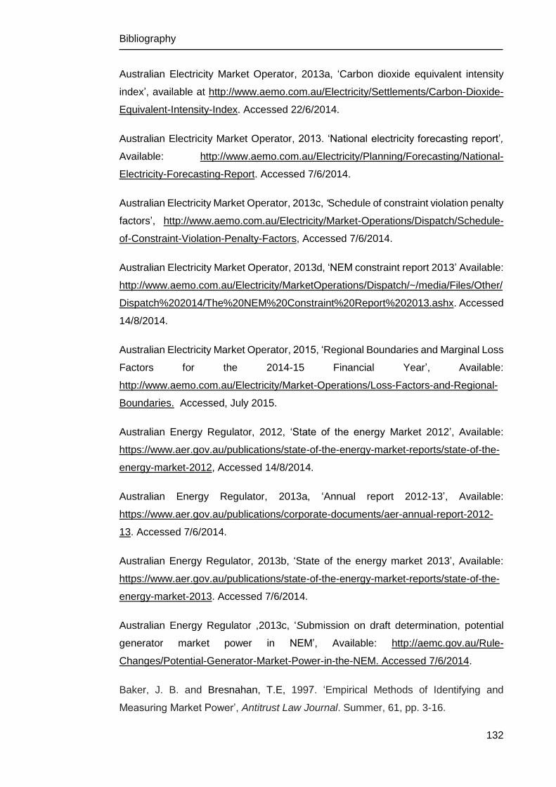
Bibliography
132
Australian Electricity Market Operator, 2013a, ‘Carbon dioxide equivalent intensity
index’, available at http://www.aemo.com.au/Electricity/Settlements/Carbon-Dioxide-
Equivalent-Intensity-Index. Accessed 22/6/2014.
Australian Electricity Market Operator, 2013. ‘National electricity forecasting report’,
Available: http://www.aemo.com.au/Electricity/Planning/Forecasting/National-
Electricity-Forecasting-Report. Accessed 7/6/2014.
Australian Electricity Market Operator, 2013c, ‘Schedule of constraint violation penalty
factors’, http://www.aemo.com.au/Electricity/Market-Operations/Dispatch/Schedule-
of-Constraint-Violation-Penalty-Factors, Accessed 7/6/2014.
Australian Electricity Market Operator, 2013d, ‘NEM constraint report 2013’ Available:
http://www.aemo.com.au/Electricity/MarketOperations/Dispatch/~/media/Files/Other/
Dispatch%202014/The%20NEM%20Constraint%20Report%202013.ashx. Accessed
14/8/2014.
Australian Electricity Market Operator, 2015, ‘Regional Boundaries and Marginal Loss
Factors for the 2014-15 Financial Year’, Available:
http://www.aemo.com.au/Electricity/Market-Operations/Loss-Factors-and-Regional-
Boundaries. Accessed, July 2015.
Australian Energy Regulator, 2012, ‘State of the energy Market 2012’, Available:
https://www.aer.gov.au/publications/state-of-the-energy-market-reports/state-of-the-
energy-market-2012, Accessed 14/8/2014.
Australian Energy Regulator, 2013a, ‘Annual report 2012-13’, Available:
https://www.aer.gov.au/publications/corporate-documents/aer-annual-report-2012-
13. Accessed 7/6/2014.
Australian Energy Regulator, 2013b, ‘State of the energy market 2013’, Available:
https://www.aer.gov.au/publications/state-of-the-energy-market-reports/state-of-the-
energy-market-2013. Accessed 7/6/2014.
Australian Energy Regulator ,2013c, ‘Submission on draft determination, potential
generator market power in NEM’, Available: http://aemc.gov.au/Rule-
Changes/Potential-Generator-Market-Power-in-the-NEM. Accessed 7/6/2014.
Baker, J. B. and Bresnahan, T.E, 1997. ‘Empirical Methods of Identifying and
Measuring Market Power’, Antitrust Law Journal. Summer, 61, pp. 3-16.

Bibliography
133
Billera, L.J., Heath, D.C. and Raanan, J., 1978. ‘Internal telephone billing rates—a
novel application of non-atomic game theory’. Operations Research, 26(6), pp.956-
965.
Blumsack, S. and Lave, L., 2003. ‘Mitigating market power in deregulated electricity
markets’, Available at http://www. andrew. cmu. edu/user/sblumsac/pivotal04.doc.
Boland, J., Filar, J.A., Mohammadian, G. and Nazari, A., 2011. ‘Australian electricity
market and price volatility’. Annals of Operations Research, pp.1-16.
Borenstein, S. and Bushnell, J., 2000. ‘Electricity restructuring: deregulation or
reregulation’. Regulation, 23, p.46.
Brennan, D. and Melanie, J., 1998. ‘Market power in the Australian power market’.
Energy Economics, 20(2), pp.121-133.
Bushnell J, Day C, Duckworth M, et al., 1999, ‘An international comparison of models
for measuring market power in electricity’. Stanford University, EMF Working Paper
17.1; Energy Modelling Forum.
Calkins, S., 1983. ‘The new merger guidelines and the Herfindahl-Hirschman Index’.
California Law Review, pp.402-429.
Conticini, C., Filar, J.A. and Ganjehlou, A.N., 2010. ‘A note on price volatility in the
Australian electricity market’. ANZIAM Journal, 51, pp.730-746.
Wen, F., 2001. ‘Market power in electricity supply’. Energy Conversion, IEEE
Transactions on, 16(4), pp.352-360.
Deza, M.M. and Deza, E., 2006. Dictionary of distances. Elsevier.
David, A. K. and Wen, F., 2000. ‘Strategic bidding in competitive electricity markets:
A Literature survey’, in Proc. Power Eng. Soc. Summer Meeting, vol. 4, Seattle, WA,
pp. 2168–2173.
Wen, F., 2001. ‘Market power in electricity supply’. IEEE Transactions on Energy
Conversion, 16(4), pp.352-360.
Exelby, M.J. and Lucas, N.J.D., 1993. ‘Competition in the UK market for electricity
generating capacity: a game theory analysis’. Energy Policy, 21(4), pp.348-354.

Bibliography
134
Fabozzi, F.J., 2007. Fixed income analysis (Vol. 6). John Wiley & Sons.
Ferrero, R.W., Shahidehpour, S.M. and Ramesh, V.C., 1997. ‘Transaction analysis in
deregulated power systems using game theory’. Power Systems, IEEE Transactions
on, 12(3), pp.1340-1347.
Green, R.J. and Newbery, D.M., 1992. ‘Competition in the British electricity spot
market’. Journal of political economy, pp.929-953.
Higgs, H., 2006. Price and volatility relationships in the Australian electricity market,
Doctoral dissertation, Queensland University of Technology.
Hu, X., Grozev, G. and Batten, D., 2005. ‘Empirical observations of bidding patterns
in Australia's National Electricity Market’. Energy Policy, 33(16), pp.2075-2086.
Hull, J.C., 2006. Options, futures, and other derivatives. Prentice Hall, New Jersey.
International Energy Agency (IEA), 2001, Energy policies of IEA countries: Australia
2001 review, Organisation for Economic Cooperation and Development, OECD
Publishing.
Jones, A.J., 1980, Game Theory: Mathematical Models of Conflict, (Chichester: Ellis
Harward Limited).
Joskow, P.L., Bohi, D.R. and Gollop, F.M., 1989. ‘Regulatory failure, regulatory
reform, and structural change in the electrical power industry’. Brookings papers on
economic activity. Microeconomics, pp.125-208.
Joskow, P. and Kahn, E., 2001. ‘A quantitative analysis of pricing behaviour in
California's wholesale electricity market during summer 2000’. In Power Engineering
Society Summer Meeting, 2001, Vol. 1, pp. 392-394.
Joskow, P.L., 2008. ‘Lessons learned from electricity market liberalization’. The
Energy Journal, 29(2), pp.9-42.
Krokhmal, P., Palmquist, J. and Uryasev, S., 2002. ‘Portfolio optimization with
conditional value-at-risk objective and constraints’. Journal of risk, 4, pp.43-68.
Luenberger, D.L., 1984. Linear and Nonlinear Programming. 2nd edition. Addison-
Wesley.

Bibliography
135
Markowitz, H.M., Todd, G.P. and Sharpe, W.F., 2000. Mean-variance analysis in
portfolio choice and capital markets (Vol. 66). John Wiley & Sons.
Mirman, L.J. and Tauman, Y., 1982. ‘Demand compatible equitable cost sharing
prices’, Mathematics of Operations Research, 7(1), pp.40-56.
Mount, T., 2001. ‘Market power and price volatility in restructured markets for
electricity’. Decision Support Systems, 30(3), pp.311-325.
Mountain, B., 2013, ‘Market power and generation from renewables: The case of wind
in the South Australian electricity market’, Econ. Energy and Environmental
Policy, vol. 2, no. 1, pp.55 -72.
National electricity Market Management company Limited, 2005, ‘Wholesale Market
Operation; Australia’s National electricity Market’, Available:
http://www.abraceel.com.br/_anexos/australiamarket-wholesalebriefing.pdf.
Accessed August 2013.
Outhred, H., 2004. ‘The Evolving Australian National Electricity Market: An
Assessment’. Power Progress: An Audit of Australia’s Electricity Reform Experiment
edited by Graeme Hodge, Valarie Sands, David Hayward and David Scott, Australian
Scholarly Publishing, Melbourne, ISBN 174097 034 9.
Pfister, R., Schwarz, K. A., Janczyk, M., Dale, R., & Freeman, J. B. 2013. ’Good things
peak in pairs: A note on the bimodality coefficient’. Frontiers in Quantitative
Psychology and Measurement, 4, 700. http://dx.doi.org/10.3389/fpsyg.2013.00700.
Quiggin, J., 2001. ‘Market-oriented reform in the Australian electricity industry’. The
Economic and Labour Relations Review, 12(1), pp.126-150.
Quiggin, J., 2004, Electricity privatisation in Victoria: Fiscal and economic impacts, in
Hodge, G., Sands. V., Hayward, D. and Scott, D., Power Progress: An Audit of
Australian reform experiment, in Australian Scholarly publishing, Melbourne, 109-123.
Rockafellar, R.T. and Uryasev, S., 2000. ‘Optimization of conditional value-at-risk’.
Journal of risk, 2, pp.21-42.
Rockafellar, R.T. and Uryasev, S., 2002. ‘Conditional value-at-risk for general loss
distributions’. Journal of banking & finance, 26(7), pp.1443-1471.

Bibliography
136
Rockafellar, R.T., Uryasev, S. and Zabarankin, M., 2006. ‘Optimality conditions in
portfolio analysis with general deviation measures’. Mathematical Programming,
108(2), pp.515-540.
Saddler, H., 1981. Energy in Australia: Politics and economics. Allen & Unwin.
Steiner, F., 2000. ‘Regulation, industry structure and performance in the electricity
supply industry’. Economics Department Working Papers no. 238. Paris: Organization
for Economic Cooperation and Development.
Samuelson, P. and Nordhaus, W., 2001. Microeconomics, McGraw-Hill, Oklahoma
City.
Sheffrin, A., 2002. ‘Predicting market power using the residual supply index’. In FERC
Market Monitoring Workshop. mimeo, Department of Market Analysis, California
ISO.
Stoft, S., 2002. ‘Power system economics’. Journal of Energy Literature, 8, pp.94-99.
Roth, A.E., 1988. The Shapley value: essays in honor of Lloyd S. Shapley. Cambridge
University Press.
Twomey, P., Green, R., Neuhoff, K. and Newbery, D., 2005. ‘A review of the
monitoring of market power: the possible roles of TSOs in monitoring for market power
issues in congested transmission systems’. MIT Center for Energy and Environmental
Policy Research.
Vassilopoulos, P., 2003. ‘Models for the identification of market power in wholesale
electricity markets’. Discussion Paper, University of Paris-Dauphine.
Von Neuman, J. and Morgenstern, O., 1944. Theory of games and economic
behavior. second ed., Princeton: Princeton University Press, 1947, 641 pp
Ward Jr, J.H., 1963. ‘Hierarchical grouping to optimize an objective function’. Journal
of the American statistical association, 58(301), pp.236-244.
Wolak, F. A. 2000. ‘Market design and price behavior in restructured electricity
markets: an international comparison’, in Takatoshi, I. and Krueger, A. O. (eds),
Deregulation and Interdependence in the Asia-Pacific Region, NBER-EASE Volume
8, NBER Books, National Bureau of Economic Research.

Bibliography
137
Wolak, F.A., 2003. ‘Measuring unilateral market power in wholesale electricity
markets: the California market, 1998-2000’. American Economic Review, pp.425-430.
Wolfram, C.D., 1999. ‘Measuring duopoly power in the British electricity spot market’.
American Economic Review, pp.805-826.