Structural Transformation and Comparative Advantage ... Kim Whang.pdf · Structural Transformation...

Structural Transformation and Comparative Advantage:

Implications for Small Open Economies

Jin-Hyuk Kim∗ Unjung Whang†

May 3, 2013

Abstract

Data from the last half century show that revealed comparative advantage in agriculture

(manufacturing) is negatively (positively) associated with the rate of decline in labor share

in agriculture. Motivated by this finding, we construct and calibrate a simple open-economy

model, where there is learning-by-doing in manufacturing and industry-supplied inputs to agri-

cultural production. We focus on the effects of comparative advantage and learning-by-doing

on structural transformation and calibrate our model to the US and the UK data to estimate key

parameters of the model. Our quantitative experiments show that holding constant other fac-

tors a small difference in a country’s comparative advantage can account for a large variation

in structural transformation for small open economies, which does not require nearly as much

differential productivity growth as in closed economy models.

JEL Classifications F43, F63, O11

Keywords: structural transformation; comparative advantage; learning-by-doing

∗Department of Economics, University of Colorado at Boulder. Email: [email protected].†Department of Economics, University of Colorado at Boulder. Email: [email protected].

1

1 Introduction

Some rich countries seem to have high productivity in agriculture than in nonagriculture (e.g.,

Australia, New Zealand, and US). Several Latin American countries (e.g., Argentina, Brazil, and

Uruguay), however, failed to achieve a high level of income during the past half-century despite

relatively high agricultural productivity, whereas some East Asian countries (e.g., Korea and Japan)

successfully transformed the economy into industrialization despite lower agricultural productivity.

To explain this pattern, economists have taken one of two approaches. Most studies consider

closed-economy models where rich countries are relatively more productive in agriculture than in

nonagriculture (e.g., Caselli 2005; Restuccia et al. 2008), whereas a smaller set of studies consider

explicitly an open-economy model where the driving force is the law of comparative advantage

(e.g., Matsuyama 1992). In this article, we refine the second stream of literature and investigate its

quantitative implications for small open economies.

A starting point for this paper is Matsuyama (1992), which suggests that the relationship be-

tween agricultural productivity and industrialization could be negative because a low agricultural

productivity implies a comparative advantage in nonagricultural sector.1 Matsuyama’s model has

been lacking solid empirical support. For instance, McMillan and Rodrik (2011) show that the

labor productivity in agricultural sector relative to nonagricultural sector exhibits a U-shaped pat-

tern as the economy develops. Specifically, they show that data from India exhibit the downward

sloping part of the curve, whereas French data shows the upward sloping part. This paper offers

a revised Matsuyama model to show that the predictions of the open-economy model are more

complicated; however, Matsuyama’s theoretical results continue to hold qualitatively, and more

importantly we show through our model calibration that the quantitative effect of comparative

advantage and learning-by-doing in open economy can be substantial.

We consider a two-sector Ricardian model similar to the one considered by Lucas (1988) and

Matsuyama (1992), where due to learning-by-doing technology the manufacturing sector’s total

1Matsuyama’s argument was based on historical evidence from Belgium and the Netherlands (Mokyr 1976) as wellas New England and the South (Field 1978; Wright 1979).

2

factor productivity (TFP) grows with its scale of production. Following Gollin et al. (2007) and

Restuccia et al. (2008), we allow agricultural sector to be modernized by using manufacturing

output as an intermediate input to its production. Different from these articles, however, we focus

on the role of comparative advantage as the driving force behind structural transformation and

growth. By showing that the model can plausibly explain the (un)successful patterns of structural

transformation in small open economies with different comparative advantages, we argue in this

paper that the open-economy view of structural transformation has a sound quantitative basis and

to more completely capture the real world can complement the dominant view discussed in the

literature that the poor countries are relatively unproductive in agriculture.

In Section 2, to motivate our study, we construct an index of revealed comparative advantage

(RCA) in agriculture as well as manufacturing, as proposed by Balassa (1965), and show that there

is a strong negative (positive) relationship between RCA in agriculture (manufacturing) and the

growth rate of decline in agriculture’s labor share in a cross-section of countries. This relationship

holds for each of the 5-year period from 1965 to 2000, for which data are available. Although this

correlation is only suggestive, it is consistent with the theoretical result in Matsuyama (1992) that

there could be a negative relationship between agricultural productivity and speed of industrializa-

tion.

In Section 3, we present our theoretical model, show conditions for industrialization to begin

in a subsistence economy, and characterize the equilibrium and the time path of a small open

economy’s structural transformation, which depends on the growth rate of world labor share in

manufacturing, the labor elasticity of output in manufacturing, and the speed of learning-by-doing

in manufacturing. In Section 4, we calibrate our model to match the US and the UK data on

agriculture’s employment share. The calibrated model, despite being simple, accounts fairly well

for the long-run growth patterns, such as the evolution of agriculture’s share of total output in the

US and the UK.

Using the 50 largest countries’ labor share data from 1961 to 2003 as a benchmark, we then

quantitatively analyze the effect of comparative advantage on structural changes. Our numerical

3

experiments show that a mere four percent initial comparative advantage in manufacturing leads to

a factor difference of three in agriculture’s employment share, and accounts for roughly 15 percent

difference in the aggregate output. Further, a five percent increase in the speed of learning-by-

doing can account for a factor difference of three in agriculture’s employment share, and about 18

percent increase in aggregate output during the sample period, while learning has little effect in a

closed economy.

This paper is related to the strand of literature that numerically investigates the effect of trade

on industrialization (e.g., Echevarria 1995; Stokey 2001; Teignier 2012). For instance, Teignier

simulates a neoclassical growth model to the structural transformation of the U.S., the U.K., and

South Korea and estimates the effect of trade on consumer welfare. The difference is that in our

model productivities evolve endogenously and we focus on the effect of comparative advantage

as well as learning in a small open economy, while in the above papers productivity growth or

technological changes are exogenous and the authors compare free trade with autarky using the

estimates of productivities.

As mentioned above, this paper aims to combine two streams of literature. One is the liter-

ature on learning-by-doing in the models of trade and growth (e.g., Krugman 1987; Boldrin and

Scheinkman 1988; Lucas 1988; Matsuyama 1992; Wong and Yip 1999), and the other is the lit-

erature on economic growth that emphasizes the role of agricultural sector (e.g., Echevarria 1997,

2008; Laitner 2000; Kongsamut et al. 2001; Gollin et al. 2004, 2007; Restuccia et al. 2008).

This paper is also related to the development literature on food problem, an observation that until

countries can reliably meet their subsistence needs, they are unable to begin the process of indus-

trialization (Schultz 1953).2

2See, also, Johnston and Mellor (1961); Fei and Ranis (1964); Chenery and Syrquin (1975); Johnston and Kilby(1975); Hayami and Ruttan (1985); and Timmer (1988). The main difference is that these articles consider closedeconomy models. We show that their main argument that an increase in agricultural productivity is essential forindustrialization to take off in the early stages of development holds in our subsistence economy (see Section 3.2) asone of two possible mechanisms.

4

2 Empirical Support

Matsuyama (1992) showed that in a small open economy agricultural productivity and industrial-

ization can be negatively related because a productive agriculture sector squeezes out the manufac-

turing sector. One could relate agriculture’s labor share with a value-added measure of (relative)

agricultural productivity to test this prediction. Such testing, however, could be imprecise. As

we will show below, relative productivity is but one factor determining a country’s comparative

advantage. For instance, if its agricultural sector uses intermediate inputs intensively and these are

available at low costs, then the country can have a comparative advantage in agriculture.

Therefore, we take an alternative approach to show the empirical correlation between compar-

ative advantage and structural transformation, where we measure a country’s comparative advan-

tage using an index of revealed comparative advantage (RCA), as proposed by Balassa (1965). The

RCA index is based on international comparisons of exports data and has been extensively used

in empirical studies in the trade literature. Specifically, a country that exports a product relatively

more intensively than the rest of the world does is defined as having a revealed comparative advan-

tage in that sector. We construct two RCA indices for agriculture and manufacturing, respectively,

using 53 countries for which export data are available in the UN Comtrade database for every

five-year between 1965 and 2000. The index is given by

RCAji =(EXP jiEXPi

)

(EXP jWEXPW

)for j = A,M ,

where j = A stands for agricultural and j = M for manufacturing sector, as defined by the SITC

framework. EXP ji is country i’s export value of sector j goods, and EXPi is country i’s total

export value. Similarly, EXP jW is the value of the world’s export in sector j, and EXPW is the

value of the world’s total export trade, where the world consists of the 53 countries in the sample.

When we match up these data with agriculture’s labor share over the same 5-year periods, the

5

sample size is reduced to 42 countries.3

Our measure of structural transformation is the (negative) growth rate of the labor share in

agriculture. To be clear, although our calibrated model economy grows due to the learning-by-

doing effect, the empirical predictions in the literature on structural transformation are formulated

in terms of labor shares. Notice that our measure is not the absolute decline in the fraction of

the labor force in agriculture, so that a decline from 0.8 of the labor force in agriculture to 0.6

is a smaller decline in terms of growth rate than one from 0.3 to 0.1. Further, the countries that

experienced large declines are not necessarily those that had large initial shares in agriculture. For

instance, in 1965, Japan and Korea had a labor share of 0.26 and 0.55, respectively, and these two

countries experienced the fastest decline in agriculture’s labor share.

Figure 1 plots the RCA index in manufacturing against the growth rate of decline in agricul-

ture’s labor share. In each subpanel, there is a clear, positive cross-sectional correlation between

the two variables, where all the slope coefficients are trivially significant at the conventional level.

As a robustness check, we plot in Figure 2 the RCA index in agriculture against the rate of decline

in agriculture’s labor share. This time there is a clear, negative correlation in each subpanel of the

figure, where the slopes are again statistically significant. While we clearly do not make any causal

interpretations, these simple correlations indicate that the law of comparative advantage may play

an important role in some countries’ structural transformation at least in the second half of the

twentieth century, when countries became more open.

[Figure 1 about here]


One might wonder if these empirical correlations may arise because the countries that experi-

ence large declines in agriculture’s labor share are countries that had large initial shares of the labor

force in agriculture, and therefore overwhelmingly poor countries. However, this is not the case in

3Data on agriculture’s labor share (as a percentage of the total labor force) come from the World Resources Institute(WRI).

6

the data. Figure 3 plots the RCA index in agriculture against per capita income and shows that there

is a strong negative relationship between the two; that is, the countries that have a low RCA index

in agriculture (hence comparative advantage in manufacturing) are not at all poor countries of the

world. As can be readily seen, several European countries as well as Japan and US are among

those in the lower right corner of the graphs. Hence, high income countries do not necessarily

have comparative advantage in agriculture as measured by RCA.


3 A Theoretical Model

3.1 Basic Structure

The economy has two sectors, agriculture and manufacturing.4 In each sector, competitive firms

produce output according to Cobb-Douglas technologies. Specifically, the agricultural sector has

two types of technologies for producing output—traditional and modern. The traditional agricul-

tural technology produces output using land and labor while the modern technology uses inter-

mediate inputs, such as chemical fertilizers and harvesting equipment, that are produced in the

manufacturing sector (see, e.g., Gollin et al. 2007). That is, agricultural production using the

traditional technology is given by

Y at = AF (L,Na

t ) = AL1−α(Nat )α,

where L is land (normalized to one) and Na is the fraction of total labor employed in the agricul-

tural sector. A represents country-specific agricultural TFP parameter that is affected by several

factors such as government policy, institution, and climate. We assume thatA is constant over time

4We abstract from non-tradable service sectors. Yi and Zhang (2011) analyze structural change in an open economymodel with three sectors, where the manufacturing employment share exhibits a hump-shaped pattern as a countrydevelops (see also Buera and Kaboski 2009; and Moro 2012).

7

so that the increase in agricultural productivity is driven by the intermediate input use (see, e.g.,

Restuccia et al. 2008 for the correlation between intermediate inputs and agricultural productivity).

As we will show below, it is necessary for the economy to start using modern agricultural

technology in order to begin industrialization process in our model. Hence, for the most part of

this paper, we will consider the modern agricultural technology, where we substitute land with

intermediate input, Xt, so output is given by

Y at = AF (Xt, N

at ) = AX1−α

t (Nat )α.

Following Lucas (1988) and Matsuyama (1992), for the sake of simplicity, we assume that the

manufacturing sector produces output using only labor. Although it would be more realistic to

incorporate capital accumulation, this assumption has proved to be useful in analyzing structural

transformation and findings relatively robust to capital accumulation (see, e.g., Restuccia et al.

2008; Alvarez-Cuadrado and Poschke 2011).

The production function in the manufacturing sector is given by

Y mt = MtF (K,Nm

t ) = MtK1−β(Nm

t )β ,

where K is capital (normalized to one), Mt represents knowledge capital, which is predetermined

but endogenous. Knowledge capitalMt (or total factor productivity in manufacturing) accumulates

as a by-product of manufacturing. Specifically, we assume that Mt = δY mt , so that Mt/Mt =

δ(Nmt )β , where δ is the (country-specific) parameter that reflects the speed of learning-by-doing.5

The learning process is exogenous to individual firms, so that each firm treats Mt as given when

making production decisions.

We assume that one unit of manufacturing output is required to produce 1/θ units of X . Under

competitive factor and output markets, θ is the price of intermediate inputs relative to manufactured

5For instance, the speed of learning-by-doing can be influenced by government policies on human capital invest-ment that impact worker’s learning on the job site.

8

goods (see, e.g., Restuccia et al. 2008). Hence, the representative farmer’s and the firm’s profit

maximization problems are given by

maxXt,Na

t

ptAX1−αt (Na

t )α − θXt − wa,tNat ,

and

maxNmt

Mt(Nmt )β − wm,tNm

t ,

respectively, where pt is the price of agricultural goods relative to manufactured goods (which

is the numeraire good in this paper), θ is the price of intermediate goods, and wa,t (wm,t) is the

agricultural (manufacturing) wage rate. Using the optimality condition, we have

wm,t = βMt(Nmt )β−1 (1)

wa,t = αAptX1−αt (Na

t )α−1 (2)

θ = (1− α)AptX−αt (Na

t )α. (3)

On the demand side, there is an infinitely-lived representative consumer, who inelastically

supply one unit of labor in each period. Labor is perfectly mobile across sectors within a country

(but immobile across countries), and factor market clearing condition ensuresNat +Nm

t = 1. Thus,

we will often denote Nmt = Nt and Na

t = 1−Nt in the following.

To incorporate the basic mechanism of structural change, we assume a functional form for

preferences of the Stone-Geary variety, where the income elasticity of demand for agricultural

goods is less than unity.6 Specifically, the representative consumer’s per-period utility is given by

U(cat , cmt ) =

cat if cat ≤ c

φ log(cat − c) + log cmt + c if cat > c,

6The observation that the slope of the Engel curve for agricultural goods is less than unity is a well-establishedempirical regularity both in cross sections of countries and in time-series data (see, e.g., Bils and Klenow 1998;Kongsamut et al. 2001).

9

where cat and cmt denote the consumption of agricultural and manufactured goods at time t, c > 0 is

a subsistence level of food consumption, and φ ∈ (0, 1) is a relative weight on food consumption.7

There is no storage, so intertemporal consumption smoothing is not possible. Thus, the represen-

tative consumer maximizes the discounted sum of utility,∑∞

t=0 ξtU(cat , c

mt ), subject to the usual

budget constraint, where ξ ∈ (0, 1) is the discount factor.

The optimality condition for the representative consumer is straightforward. When cat ≤ c,

individuals only consume food. When cat > c, the representative consumer first allocates income I

to meet the subsistence consumption of food, and then the remaining to both goods, so that

cat = c+φ

pt(1 + φ)(I − ptc)

cmt =1

1 + φ(I − ptc).

Hence, assuming that the consumer has enough income to purchase more than c unit of food,

the optimality condition is given by

cat = c+φ

ptcmt . (4)

3.2 Subsistence Economy

In this subsection, we briefly discuss how a country starts the development process in our model.

There are two possibilities for allocating labor in the subsistence economy. One possibility is

that farmers produce agricultural output using the traditional technology. Since consumers derive

no utility from consuming manufactured goods in this state, there is no labor allocation in the

manufacturing sector. The other possibility is that farmers produce agricultural goods using the

modern technology, in which case there will be some labor allocation in the manufacturing sector;

however, all manufactured goods will be used as intermediate inputs to agricultural production in

a closed economy.

7As is common in this literature, we ignore the problem that the instantaneous utility is lowered when cat increasesfrom c to a slightly higher number.

10

Hence, a subsistence economy will optimally adopt the modern technology if and only if the

consumer’s lifetime utility from using the modern agricultural technology is greater than that from

using the traditional technology. This holds if

M0 ≥(β(1− α) + α

β(1− α)

)β (β(1− α) + α

α

) α1−α

, (5)

the derivation of which is relegated to the Appendix.8

The above condition implies that if the initial value of manufacturing productivity, M0, is

sufficiently large, then even though a country’s initial agricultural productivity is relatively low,

labor force will flow out of agriculture before agricultural productivity rises above the subsistence

level. To be precise, the labor allocation during this gestation period will be constant, Nmt /N

at =

(β − βα)/α, while food consumption level increases gradually as Mt grows over time. Once

consumption reaches the subsistence level, consumers begin to consume manufactured goods and

additional labor will flow out of agriculture into manufacturing sector.9

If the above inequality is not satisfied, then labor would be entirely devoted to the traditional

agricultural sector, and we need an exogenous increase in either agricultural productivity or man-

ufacturing productivity to jump-start industrialization. In particular, as in the conventional ar-

guments, whenever the increase in agricultural productivity pushes the economy above the sub-

sistence level, structural transformation will begin. However, in light of the empirical evidence

suggested above, early manufacturing productivity seems to play an important role in explaining

relatively recent development experiences of some small open economies.

8This makes the conservative assumption that the learning-by-doing parameter δ is sufficiently small, so that thelifetime utility from using the modern agricultural technology will not go to infinity. If δ is large enough to satisfy

ξ

(1 + δ

(β(1−α)

β(1−α)+α

)β)1−α

≥ 1, then this suffices to use the modern agricultural technology under subsistence

conditions.9This argument seems consistent with the finding by Alvarez-Cuadrado and Poschke (2011) that productivity

improvements in the nonagricultural sector were the main driver of structural change before 1960.

11

3.3 Closed Economy

Here we characterize the equilibrium path after a country begins structural transformation moving

beyond the subsistence level. Agricultural production uses the modern technology, so the repre-

sentative consumer consumes both agricultural and manufactured goods. Since the economy is

closed, the following market clearing conditions hold.

cat = Y at = AX1−α

t (1−Nt)α

cmt = Y mt − θXt = MtN

βt − θXt.

Combining these with equation (4) yields

AX1−αt (1−Nt)

α = c+φ

pt

(MtN

βt − θXt

). (6)

The no-arbitrage condition in the competitive labor market holds in each period (i.e., wm,t =

wa,t for all t), so that

βMt(Nt)β−1 = αAptX

1−αt (1−Nt)

α−1. (7)

Equations (3), (6), and (7) may now be solved for the three unknowns {Xt, pt, Nt}. From (3)

and (7), we have

pt =1

A

(1− αθ

)α−1(β

α

)αMα

t N(β−1)αt (8)

Xt =

(1− αθ

)(β

α

)MtN

β−1t (1−Nt). (9)

Substituting (6) with (8) and (9) yields

(1−Nt)N(β−1)(1−α)t

(β

α

)1−α

(1+φ(1−α))−φ(β

α

)−αN

(β−1)(1−α)+1t =

c

A

(1− αθ

)α−1Mα−1

t .

(10)

Notice that the left-hand side of equation (10) is strictly decreasing in Nt, and the right-hand

12

side is a positive number. Further, the left-hand side tends to infinity as Nt approaches zero,

and it is negative at Nt = 1. Since Mt on the right-hand side grows over time at a rate δNβt ,

equation (10) has a unique solution in Nt ∈ (0, 1), which depends on the parameters of the model,

{A, c, θ, α, β, φ}, and Mt.

Since Mt/Mt = (Mt+1 −Mt)/Mt = δNβt , it follows that Mt = M0

∏tτ=1(1 + δNβ

τ−1) for

t ≥ 1. Therefore, the labor share in manufacturing in each period t after industrialization can be

written as

Nt = v [Mt(M0, δ, β);A, c, θ, α, β, φ] .

The function v exhibits standard features that explain a country’s structural transformation.

For instance, holding other factors constant, a higher initial manufacturing productivity, M0, pulls

the labor force from the agricultural sector. A higher agricultural productivity, A, increases the

labor share in manufacturing as well because it substitutes for the labor demand in agriculture.

Relatedly, the labor’s share in manufacturing is negatively related to θ, the efficiency parameter or

the conversion ratio of manufacturing output to intermediate inputs, and c, the subsistence level of

food consumption. A technological progress in the intermediate-input production, through lower

θ, can push labor into the manufacturing sector.

It is also true that a country with more efficient learning technology, δ, can experience more

rapid industrialization in which labor flows out of agriculture to manufacturing sector. However, as

we will show in our calibration, the quantitative effect of learning-by-doing is limited in a closed

economy whereas a relatively small difference in δ can lead to a large difference in a country’s

structural transformation in an open economy setting. Even if we assume that knowledge spillovers

across countries occur over time (Lucas 2009), so the country that starts industrialization later

tends to have a higher value of δ, our analysis below suggests that the convergence effect may be

attenuated by comparative advantage in agriculture.

13

3.4 Open Economy

Consider a small open economy (called home), which is the country described above, while the

rest of the world has the same preferences and production functions as home and its variables are

labeled by an asterisk (∗). The two countries only differ by agricultural productivity, A, initial

knowledge capital in manufacturing, M0, and the intermediate input price, θ. The home country

takes prices as given, and this means that the technology to transform intermediate inputs to agri-

cultural output is the same at home and in the rest of the world. Labor is immobile across countries,

and we assume that learning-by-doing effects do not spill over across countries.

Suppose that these countries are allowed to trade with each other. In the absence of interna-

tional capital market, the world economy evolves just as we described in the previous subsection.

Consumers maximize their instantaneous utility, and firms in each sector maximize profit in the

competitive factor and output markets. Characterizing the equilibrium quantities, however, is un-

necessary for this section’s purpose. Instead, we focus on the equilibrium path of structural trans-

formation in terms of labor share in agriculture. Denoting the world (relative) prices of agricultural

goods and intermediate inputs as p∗t and θ∗, respectively, the following first-order conditions hold.

βM∗t (N∗t )β−1 = αA∗p∗tX

∗1−αt (1−N∗t )α−1 (11)

θ∗ = (1− α)A∗p∗tX∗−αt (1−N∗t )α. (12)

Given the properties of the production functions, trading partners will not completely special-

ize. Under the assumption of free trade (which we discuss below), the home country’s labor share

in manufacturing is determined by the two equations above together with (3) and (7). Specifically,

combining (11) and (7) yields

Mt

AX1−αt

Nβ−1t

(1−Nt)α−1=

M∗t

A∗X∗1−αt

N∗β−1t

(1−N∗t )α−1. (13)

14

From (12) and (3), we have

Xt

X∗t=

(A

A∗

) 1α(

1−Nt

1−N∗t

). (14)

Finally, combining (13) and (14) yields

(Nt

N∗t

)β−1=

(A

A∗

) 1α M∗

t

Mt

. (15)

Suppose at time t the home country opens up to trade. Our measure of comparative advantage

is the ratio of Hicks-neutral TFP in the two sectors, which is based on the gross output production

model. That is, the intermediate input is not explicitly separated from TFP parameters. Given that

the intermediate input prices are equalized in our simple model, the standard definition of compar-

ative advantage applies as long as input conversion technologies are the same across countries (see,

e.g., Jones 1961). Therefore, the home country has a comparative advantage in manufacturing if

and only ifMt

AX1−αt

>M∗

t

A∗X∗1−αt

.

From equation (13), we conclude that

Nt T N∗t if and only ifMt

AX1−αt

TM∗

t

A∗X∗1−αt

.

That is, the labor’s share in manufacturing sector must be greater for the home country than

that for the rest of the world, so that the home country can have a comparative advantage in manu-

factured goods. Notice that the comparative advantage term is influenced by the intermediate input

use as well as relative productivity as we discussed in the previous section.

From the free trading equilibrium condition (15), we find the time path of the labor share in the

15

home country by differentiating (15) with respect to time.

Nt

Nt

=N∗tN∗t

+1

1− β

(Mt

Mt

− M∗t

M∗t

)(16)

=N∗tN∗t

+δ

1− β(Nβ

t −N∗βt ).

Thus, in a small open economy, the growth rate of labor share in manufacturing sector depends

on the growth rate of the world’s labor share in manufacturing and comparative (dis)advantage

in manufacturing. The labor share in manufacturing in the home country will increase at a faster

rate than that in the rest of the world if its initial labor share in manufacturing is larger than that

in the world (i.e., Nt > N∗t ), hence, a comparative advantage in manufacturing. The effect of

comparative advantage depends on the speed of learning-by-doing, δ, and the labor elasticity of

output in manufacturing, β, (which are assumed to be identical across countries). In particular, if

δ and β are sufficiently large, then the country that has a comparative advantage in agriculture can

experience de-industrialization (i.e., Nt/Nt < 0) as put forth by Matsuyama (1992).

Another difference from the closed economy models such as the one analyzed by Restuccia

et al. (2008) is that in this paper export-oriented policies have no implication for small open

economies’ structural transformation. Specifically, the home country’s time path of the labor share

in manufacturing (i.e., equation (16) above) is unaffected by import tariffs (or export subsidies) on

manufactured goods. That is, suppose the domestic price of manufactured goods (the numeraire

good) increases from 1 to 1 + τ , where τ represents the tax. Then the relative domestic prices of

agricultural and intermediate goods will decrease to pt/(1 + τ) and θ/(1 + τ), respectively, so that

in equilibrium pt = p∗t (1 + τ) and θ = θ∗(1 + τ) hold. It can be easily shown that the differential

equation (16) remains the same as long as the tax is held constant across time.

The logic behind this result is that the optimal allocation of labor in a small open economy is

completely determined by the world prices, which small open economies take as given. Hence,

our model supports the view that the export-oriented government policies did not contribute much

16

to the development experience of the Asian tigers (i.e., Hong Kong, Singapore, South Korea, and

Taiwan). More importantly, the model predicts path dependence in economic development. That

is, if whether industrialization begins depends on the level of initial manufacturing productivity

relative to that of the rest of the world (which determines the comparative advantage), then as more

countries become industrialized, it may become increasingly harder for the remaining agricultural

economies to satisfy this initial condition for successful structural changes to take place.

4 Numerical Experiments

4.1 Closed Economy

The length of a time period is set to one year. To focus on the effect of comparative advantage on

industrialization, we normalize the values of A, M0, θ, and c to one, which means that if the agri-

cultural sector uses the traditional technology it will produce exactly the subsistence needs of the

population, and hence industrialization can begin.10 The parameter φ determines the expenditure

share as well as the long-run share of employment in agriculture. Following Gollin et al. (2004),

we set φ = 0.003. Next, we choose the value of 1 − α to match the intermediate-input-to-output

ratio in agriculture. The data from the U.S. Department of Commerce’s (1975) Historical Statistics

suggest that this ratio is 0.39, so we set α = 0.61. Accounting for intangible capital investment,

we set the labor share parameter β in manufacturing equal to 0.5.11

Next, we estimate the value of δ such that the model matches the evolution of agriculture’s

employment share as accurately as possible. That is, given the data on employment shares, we

calculate annual time series by cubic interpolation, and then choose the value of δ that minimizes

the sum of squares of the distance between the data and the model’s prediction during the time

10Different values of the subsistence level of consumption would have implicaitons for different starting date ofstructural transformation, the quantitative implication of which in this paper is straightforward and hence omitted. Seealso Gollin et al. (2007) for implications of agricultural productivity on the onset of industrialization.

11Corrado et al. (2009) estimate that the average investment in intangible capital was around 15% of the outputduring 2000-2003. Gollin et al. (2007) also set the (physical and intangible) capital share paramter equal to 0.5, whichis higher than the conventional one-third level.

17

period when the labor’s share in agriculture decreases from 70 to 20 percent. Admittedly, this may

appear to be somewhat arbitrary, but it reflects a balance between power consideration and a desire

to focus on the rapid industrialization period. Thus, δ = arg min∑

t∈{t:0.2≤St≤0.7}[St−Nat ]2, where

St is the labor share data and Nat is the value generated by the model. The employment as well as

output share data are taken from Kuznets (1966) and International Historical Statistics (Mitchell

1992, 1993).12

First, we calibrate the model to UK data on labor’s share in agriculture. The parameter δ is

estimated to be 0.050. By construction, the calibrated model matches the data very well. Figure

4 plots the time-series data on agriculture’s labor share from 1775 to 1995 together with the time

path predicted by the model. Given the parametrization chosen, the calibration implies that the first

year in which labor started flowing out of agriculture is approximately 1700, which is in line with

Gollin et al.’s (2007) estimate. The model performs fairly well in replicating the long-run pattern

of agriculture’s share of output even though the model was not calibrated to match this dimension.

Figure 5 shows the output share of agriculture over time. Despite its parsimonious structure, the

model appears to provide a good description of agriculture’s share of labor and output in the UK

data.



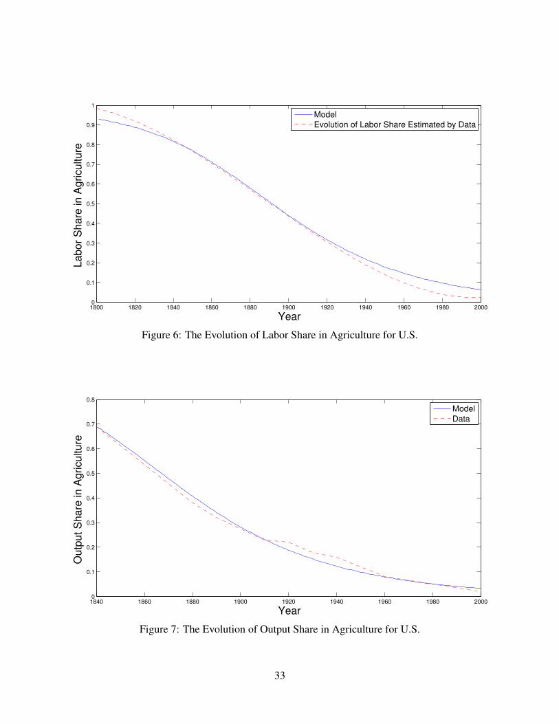
We also calibrated the model to US data on labor’s share in agriculture. Following the same

procedure as above, the parameter δ is estimated to be 0.062, which is greater than the δ in the

U.K. Figure 6 plots the time-series labor share in agriculture in the U.S. from 1800 to 2000 and the

model’s prediction. The model predicts that the transition during which labor share in agriculture

drops from 70 to 20 percent in the U.S. occurs between approximately 1860 and 1940, while the

same structural change occurred in the calibrated UK economy between 1765 to 1878. Hence,

12In the data, manufacturing sector includes mining, public utilities, transportation, and communications. Servicesare not included in calculation.

18

the model can explain the fact that the US economy experienced structural changes in a shorter

time period than the UK economy did. Figure 7 plots the agriculture’s output share in the US

data and the time path from the calibration. The model captures important aspects of structural

transformation reasonably well.



4.2 Open Economy

We now use the model to examine the implications for small open economies, where we focus

on the effect of comparative advantage and learning-by-doing. In what follows, we aggregate

the 50 largest countries’ labor share data over the period 1961-2003 and use it as representing

the world economy. Each country’s labor share data is taken from the World Resources Institute

(WRI). During this period, the agriculture’s labor share of the world economy decreased from 60

to 42 percent. Given the world’s labor share in agriculture, the equilibrium path of a small open

economy’s labor share in agriculture is determined by equation (16) above. Figure 8 displays a

series of numerical experiments where the home country differs from the rest of the world only

by the initial value of manufacturing labor share. In what follows, we set δ∗ = 0.055 and M∗0 =

M0 = 4.13


Figure 8 shows that comparative advantage alone can explain a large variation in the secular de-

cline in agriculture’s labor share. That is, holding constant other parameter values across countries,

a small (in the range of one to four percent) difference in a country’s initial comparative advantage

leads to a dramatically different time trend of agriculture’s labor share for a small open economy.13The world’s learning-by-doing parameter value is taken between the above two estimates for the US and the

UK. The initial manufacturing productivity in 1960 for both home and the world reflects the equilibrium path of thebenchmark closed economy, so that M∗0 is the implied productivity when the agriculture’s labor share is 0.6.

19

Specifically, if a country has an initial, four percent comparative advantage in manufacturing rela-

tive to the world, then its employment share in agriculture will fall from 0.60 to 0.13 between 1961

and 2003. In contrast, a county with the same small comparative disadvantage in manufacturing

can experience slowdown or even deindustrialization.

The simulation results seem to accord well with the actual data. In Figure 9, we plot the actual

time path of the countries whose labor share in agriculture in 1961 is close to 0.6, the initial value

of the simulated open economy above. These comprise 20 countries with agriculture’s labor share

between 0.55 and 0.65 in 1961. Figure 9 shows that the time path of structural transformation

varies widely by countries, which can be at least partially accounted for by the simulated open

economy in Figure 8. Given the empirical correlation presented in Section 2, this demonstrates

that the forces of comparative advantage can plausibly explain the experience of some late-starting

countries in the second half of the twentieth century.


Given our characterization of structural transformation by equation (16), one might think that

the data can also be explained by assuming differential TFP growth. It is partly true that different

learning-by-doing parameters can generate similar patterns as explained by comparative advantage.

However, the differential rate of learning (hence productivity growth) needed to explain the same

amount of variation in closed-economy models would be much higher than that required in small

open economies. To show this, suppose that the home country’s initial labor share in manufacturing

is the same as that of the rest of the world (i.e., N0 = N∗0 ), but its learning technology is different

from the world’s. In this case the equilibrium path of the home country’s labor share in agriculture

is still defined by equation (16), where the new differential equation is now given by

Nt

Nt

=N∗tN∗t

+1

1− β(δNβ

t − δ∗N∗βt ) (17)

20

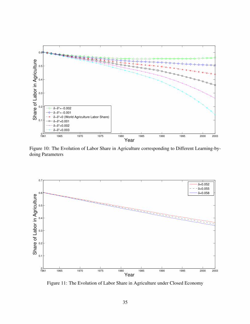
Figure 10 shows that a small (around five percent) increase in the speed of learning-by-doing

can explain just as much variation in secular decline of agriculture’s employment share in the ab-

sence of any initial comparative advantage in manufacturing. However, when we simulate a closed

economy model where parameter values are the same as those used for the world economy ex-

cept that δ is varied, learning-by-doing (hence productivity differential alone) could not generate

a meaningful variation. Figure 11 shows the time path of this simulated closed economy, where

a once-and-for-all increase in δ from 0.055 to 0.058 makes only a minor difference to the agri-

culture’s share of employment, whereas in Figure 10 the same change leads to a factor difference

of three in 40 years. Therefore, the above results cannot be explained away by differential TFP

growth.



Figure 12 and Figure 13 show the total output or GDP of the home country (i.e., p∗tYat −

θ∗Xt + Y mt ) for the respective scenarios considered above. The model predicts that the small

open economy’s output increases almost fivefold between 1961 and 2003, with an average annual

growth rate of four percent. This seems to be consistent with the development experience of the

Newly Industrialized Economies. Further, starting with the same initial conditions, a relatively

small difference in comparative advantage or learning technology can account for up to 15 percent

difference in total output variation by the end of the 40-year period. This suggests that structural

transformation has a modest but economically significant effect on growth.14



14These figures seem consistent with McMillan and Rodrik (2011)’s finding that holding constant sectoral produc-tivity levels in poor countries counterfactual reallocation of labor that matches the pattern observed in the rich countriescan account for as much as one fifth of the productivity gap.

21

Finally, Figure 14 and Figure 15 display the value-added per worker in manufacturing relative

to agriculture in the small open economy. Figure 14 shows that a comparative advantage in manu-

facturing has an initial, level effect on the relative productivity; however, it has little growth effect

over time. On the other hand, Figure 15 shows that an increase in learning-by-doing parameter has

some growth effect on relative productivity; however, the magnitude of this growth effect is much

smaller than the effect of comparative advantage. This relatively small variation is also consistent

with the observation that the relative productivity has been stable over time for developed countries

like the US and UK (see, e.g., Gollin et al. 2004).



5 Conclusion

The literature has uncovered some of the most important mechanisms of structural transformation

in a closed economy, such as an income elasticity of the demand for agricultural goods less than

one and faster total factor productivity growth in agriculture relative to other sectors of the econ-

omy. Our results partly confirm this conventional wisdom, but we argue that these mechanisms

may not completely capture structural transformation and lock-in in an increasingly globalized

economy. In particular, after the onset of industrialization comparative advantage seems to be an

important consideration, which we supported by showing that our simple calibrated open economy

can generate a plausible time path of labor share in agriculture.

Our quantitative analysis suggests that countries with relatively productive manufacturing sec-

tors move rapidly to specialize in manufacturing, while those with comparative advantage in agri-

culture will experience little structural transformation. We believe that these account well for the

growth miracles in the four East Asian tigers and the lock-in of several currently middle-income

countries in Latin America and Southeast Asia. Our small open economy model is not at odds with

22

(but rather complement) the development experience of the currently rich countries as this paper

does not intend to explain the early industrialization before the 20th century, when closed economy

models may do a better job of explaining structural transformation.

References

[1] Alvarez-Cuadrado, F., Poschke, M., 2011. Structural change out of agriculture: labor push

versus labor pull. American Economic Journal: Macroeconomics 3(3): 127–158.

[2] Balassa, B., 1965. Trade liberalisation and “revealed” comparative advantage. Manchester

School 33(2): 99–123.

[3] Bils, M., Klenow, P.J., 1998. Using consumer theory to test competing business cycle models.

Journal of Political Economy 106(2): 233–261.

[4] Boldrin, M., Scheinkman, J.A., 1988. Learning by doing, international trade and growth: a

note. In: Anderson P., et al. (Eds.), The Economy as an Evolving Complex System. Addison

Wesley, New York.

[5] Buera, F.J., Kaboski, J.P., 2009. Can traditional theories of structural change fit the data?

Journal of the European Economic Association 7: 469–477.

[6] Caselli, F., 2005. Accounting for cross-country income differences. Handbook of Economic

Growth 1A: 679–741.

[7] Chenery, H., Syrquin, M., 1975. Patterns of Development: 1950-1970. Oxford University

Press, London.

[8] Corrado, C., Hulten, C., Sichel, D., 2009. Intangible capital and U.S. economic growth. Re-

view of Income and Wealth 55: 661–685.

23

[9] Echevarria, C., 1995. Agricultural development vs. industrialization: Effects of trade. Cana-

dian Journal of Economics 28(3): 631–647.

[10] ———, 1997. Changes in sectoral composition associated with economic growth. Interna-

tional Economic Review 38(2): 431–452.

[11] ———, 2008. International trade and the sectoral composition of production. Review of

Economic Dynamics 11(1): 192–206.

[12] Fei, J.C.H., Ranis, G., 1964. Development of the Labour Surplus Economy: Theory and

Policy. Richard D. Irwin for the Economic Growth Center, Yale University.

[13] Field, A.J., 1978. Sectoral shift in Antebellum Massachusetts: A reconsideration. Explo-

rations in Economic History 15(2): 146–171.

[14] Gollin, D., Parente, S.L., Rogerson, R., 2004. Farmwork, homework and international pro-

ductivity differences. Review of Economic Dynamics 7(4): 827–850.

[15] ———, ———, ———, 2007. The food problem and the evolution of international income

levels. Journal of Monetary Economics 54: 1230–1255.

[16] Hayami, Y., Ruttan, V.W., 1985. Agricultural Development: An International Perspective.

Johns Hopkins University Press, Baltimore.

[17] Johnston, B.F., Mellor, J.W., 1961. The role of agriculture in economic development. Ameri-

can Economic Review 51(4): 566–593.

[18] Johnston, B.F., Kilby, P., 1975. Agriculture and Structural Transformation: Economic Strate-

gies in Late-Developing Countries. Oxford University Press, London.

[19] Jones, R.W., 1961. Comparative advantage and the theory of tariffs: A multi-country, multi-

commodity model. Review of Economic Studies 28(3): 161–175.

24

[20] Kongsamut, P., Rebelo, S., Xie, D., 2001. Beyond balanced growth. Review of Economic

Studies 68(4): 869–882.

[21] Krugman, P., 1987. The narrow moving band, the Dutch disease, and the competitive con-

sequences of Mrs. Thatcher: Notes on trade in the presence of dynamic scale economies.

Journal of Development Economics 27(1–2): 41–55.

[22] Kuznets, S., 1966. Modern Economic Growth. Yale University Press, New Haven.

[23] Laitner, J., 2000. Structural change and economic growth. Review of Economic Studies 67(3):

545–561.

[24] Lucas, R.E., 1988. On the mechanics of economic development. Journal of Monetary Eco-

nomics 22(1): 3–42.

[25] ———, 2009. Trade and the diffusion of the Industrial Revolution. American Economic

Journal: Macroeconomics 1(1): 1–25.

[26] Matsuyama, K., 1992. Agricultural productivity, comparative advantage, and economic

growth. Journal of Economic Theory 58(2): 317–334.

[27] McMillan, M.S., Rodrik, D., 2011. Globalization, structural change and productivity growth.

NBER Working Paper No. 17143.

[28] Mitchell, B.R., 1992. International Historical Statistics: Europe 1750–1988. Stockton Press,

New York.

[29] Mitchell, B.R., 1993. International Historical Statistics: The Americas 1750–1988. Stockton

Press, New York.

[30] Mokyr, J., 1976. Industrialization in the Low Countries, 1795–1850. Yale University Press,

New Haven.

25

[31] Moro, A., 2012. The structural transformation between manufacturing and services and the

decline in the US GDP volatility. Review of Economic Dynamics 15(3): 402–415.

[32] Restuccia, D., Yang, D.T., Zhu, X., 2008. Agriculture and aggregate productivity: A quanti-

tative cross-country analysis. Journal of Monetary Economics 55: 234–250.

[33] Schultz, T.W., 1953. The Economic Organization of Agriculture. McGraw-Hill, New York.

[34] Stokey, N.L., 2001. A quantitative model of the British industrial revolution, 1780–1850.

Carnegie-Rochester Conference Series on Public Policy 55(1): 55–109.

[35] Teignier, M., 2012. The role of trade in structural transformation. Mimeo.

[36] Timmer, C.P., 1988. The agricultural transformation. In: Chenery, H., Srinivasan, T.N. (Eds.),

Handbook of Development Economics, vol. 1. Elsevier, Amsterdam, pp. 275–331.

[37] U.S. Department of Commerce, 1975. Historical Statistics of the United States: Colonial

Times to 1970. Bureau of the Census, Washington D.C.

[38] Wong, K., Yip, C.K., 1999. Industrialization, economic growth, and international trade. Re-

view of International Economics 7(3): 522–540.

[39] Wright, G., 1979. Cheap labor and Southern textiles before 1880. Journal of Economic His-

tory 39(3): 655–680.

[40] Yi, K.-M., Zhang, J., 2011. Structural change in an open economy. Mimeo.

26

6 Appendix

Condition (5), which is sufficient to start industrialization, is derived from comparing the lifetime

utility from consuming agricultural goods using only the traditional technology with that from

consuming agricultural goods using the modern technology where all manufactured goods are

used as intermediate inputs. This gives a sufficient condition because if the modern technology

is used in agriculture, then there will be some finite time at which the consumer starts consuming

manufactured goods and achieve a higher level of utility.

In the former case, since all labor is allocated to agricultural sector (i.e., Nt = 0 for all t),

agricultural output is Y at = A(1 − Nt)

α = A. The lifetime utility is thus U =∑∞

t=0 ξtcat =∑∞

t=0 ξtA = A/(1 − ξ). In the latter case, agricultural output is Y a

t = AX1−αt (1 − Nt)

α =

A(MtNβt )1−α(1−Nt)

α. The first welfare theorem, that competitive equilibrium is efficient, implies

that the consumer’s lifetime utility is maximized with respect to labor allocation. Hence, the

maximization problem, max∑∞

t=0 ξtA(MtN

βt )1−α(1−Nt)

α, yields optimal labor allocation in the

manufacturing sector,

Nt =β(1− α)

β(1− α) + α.

Notice that Mt/Mt = (Mt+1 −Mt)/Mt = δNβt . Rearranging yields

Mt+1 = Mt

(1 + δ

(β(1− α)

β(1− α) + α

)β).

Therefore, the lifetime utility is

U = A

(β(1− α)

β(1− α) + α

)β(1−α)(α

β(1− α) + α

)α ∞∑t=0

ξtM1−αt

= A

(β(1− α)

β(1− α) + α

)β(1−α)(α

β(1− α) + α

)αM1−α

0

∞∑t=0

ξt

[(1 + δ

(β(1− α)

β(1− α) + α

)β)t]1−α.

If ξ(

1 + δ(

β(1−α)β(1−α)+α

)β)1−α

≥ 1, then the lifetime utility explodes to infinity.

27

If ξ(

1 + δ(

β(1−α)β(1−α)+α

)β)1−α

< 1, then the lifetime utility is

U =A(

β(1−α)β(1−α)+α

)β(1−α) (α

β(1−α)+α

)αM1−α

0

1− ξ(

1 + δ(

β(1−α)β(1−α)+α

)β)1−α .

Therefore, the lifetime utility using the modern technology is greater than not using it if and

only if (β(1−α)

β(1−α)+α

)β(1−α) (α

β(1−α)+α

)αM1−α

0

1− ξ(

1 + δ(

β(1−α)β(1−α)+α

)β)1−α >1

1− ξ.

Since 1 + δ(

β(1−α)β(1−α)+α

)β> 1, a sufficient condition for the above inequality to hold is

(β(1− α)

β(1− α) + α

)β(1−α)(α

β(1− α) + α

)αM1−α

0 ≥ 1.

Rearranging yields condition (5).

28

ARG

AUS

AUT

BRA

CAN

CHE

CHL

COLCRI

DEU

DNK

ECU

EGY

ESP

FIN

FRA

GBR

GRCGTM

HND

HUN

IRL

ISR

ITA

JPN

KOR

MEX

MYSNIC

NLDNOR

NZLPANPERPHL

PRT

PRY

SLV

SWE

THATUR

USA

ARG

AUS

AUT

BRA

CAN

CHE

CHL

COL

CRI

DEU

DNK

ECU

EGY

ESP

FIN

FRA

GBR

GRC

GTM

HND

HUN

IRL

ISR

ITAJPN

KOR

MEX

MYSNIC

NLD

NOR

NZLPANPER

PHL

PRT

PRY

SLV

SWE

THATUR

USA

ARGAUS

AUT

BRA

CAN

CHE

CHL

COL CRI

DEU

DNK

ECU

EGY

ESPFINFRA

GBR

GRC

GTM

HND

HUN

IRL

ISR

ITAJPN

KOR

MEX

MYSNIC

NLD

NOR

NZLPANPER

PHL

PRT

PRY

SLV

SWE

THA

TUR

USA

ARGAUS

AUT

BRA

CAN

CHE

CHLCOL

CRI

DEU

DNK

ECU

EGY

ESPFINFRA

GBR

GRC

GTM

HND

HUN

IRL

ISRITAJPN

KOR

MEX

MYS

NIC

NLD

NOR

NZL

PAN

PER

PHL

PRT

PRY

SLV

SWE

THATUR

USA

ARGAUS

AUT

BRA

CAN

CHE

CHL COLCRI

DEU

DNK

ECU

EGY

ESPFINFRA

GBR

GRC

GTM

HND

HUNIRL

ISRITA

JPNKOR

MEX

MYS

NIC

NLD

NOR

NZL

PAN

PER

PHL

PRT

PRY

SLV

SWE

THA

TUR

USA

ARG

AUS

AUT

BRA

CAN

CHE

CHL

COL

CRI

DEU

DNK

ECU

EGY

ESPFIN

FRA

GBR

GRC

GTM

HND

HUNIRL

ISRITA

JPNKOR

MEXMYS

NIC

NLDNOR

NZLPAN

PER

PHL

PRT

PRY

SLV

SWE

THATUR

USA

ARG

AUS

AUT

BRA

CAN

CHE

CHL

COL

CRI

DEU

DNK

ECU

EGY

ESPFIN

FRAGBR

GRC

GTM

HND

HUNIRL

ISRITAJPNKOR

MEXMYS

NIC

NLDNOR

NZL

PAN

PER

PHL

PRT

PRY

SLV

SWE

THATURUSA

0.5

11

.50

.51

1.5

0 .2 .4

0 .2 .4 0 .2 .4 0 .2 .4

1965−1970 1970−1975 1975−1980 1980−1985

1985−1990 1990−1995 1995−2000

Re

ve

ale

d C

A in

Ma

nu

factu

rin

g

Growth Rate of Labor Share in Manufacturing

Figure 1: Relationship between RCA in Manufacturing and Growth Rate of Manufacturing Labor Share

29

ARGAUS

AUT

BRA

CAN

CHE

CHL

COLCRI

DEU

DNK

ECU

EGY

ESP

FIN

FRAGBR

GRCGTMHND

HUN

IRL

ISR

ITAJPN

KOR

MEXMYSNIC

NLDNOR

NZLPANPERPHL

PRT

PRYSLV

SWE

THATUR

USA

ARG

AUS

AUT

BRA

CAN

CHE

CHL

COLCRI

DEU

DNK

ECU

EGY

ESPFINFRA

GBR

GRC

GTM

HND

HUN

IRL

ISR

ITAJPN

KOR

MEX

MYSNIC

NLDNOR

NZLPANPER

PHL

PRT

PRY

SLV

SWE

THATUR

USA

ARGAUS

AUT

BRA

CAN

CHE

CHL

COL CRI

DEU

DNK

ECU

EGY

ESPFINFRA

GBR

GRC

GTM

HND

HUN

IRL

ISR

ITAJPN

KOR

MEX

MYSNIC

NLD

NOR

NZLPANPER

PHL

PRT

PRY

SLV

SWE

THATUR

USA

ARGAUS

AUT

BRA

CAN

CHE

CHLCOL

CRI

DEU

DNK

ECU

EGY

ESPFINFRA

GBR

GRC

GTM

HND

HUN

IRL

ISRITAJPN

KOR

MEX

MYS

NIC

NLDNOR

NZL

PAN

PER

PHL

PRT

PRY

SLV

SWE

THATUR

USA

ARGAUS

AUT

BRA

CAN

CHE

CHLCOLCRI

DEU

DNK

ECU

EGY

ESPFINFRA

GBR

GRC

GTM

HND

HUNIRL

ISRITA

JPNKOR

MEX

MYS

NIC

NLD

NOR

NZL

PAN

PER

PHL

PRT

PRY

SLV

SWE

THA

TUR

USA

ARG

AUS

AUT

BRA

CAN

CHE

CHL

COL

CRI

DEU

DNK

ECU

EGY

ESPFIN

FRA

GBR

GRC

GTM

HND

HUNIRL

ISRITA

JPNKOR

MEX

MYS

NIC

NLD

NOR

NZLPAN

PER

PHL

PRT

PRY

SLV

SWE

THA

TUR

USA

ARG

AUS

AUT

BRA

CAN

CHE

CHL

COL

CRI

DEU

DNK

ECU

EGY

ESP

FINFRA

GBR

GRC

GTM

HND

HUNIRL

ISRITA

JPNKOR

MEX

MYS

NIC

NLDNOR

NZL

PAN

PER

PHL

PRT

PRY

SLV

SWE

THATUR

USA

02

46

02

46

0 .2 .4

0 .2 .4 0 .2 .4 0 .2 .4

1965−1970 1970−1975 1975−1980 1980−1985

1985−1990 1990−1995 1995−2000

Re

ve

ale

d C

A in

Ag

ricu

ltu

re

Growth Rate of Labor Share in Manufacturing

Figure 2: Relationship between RCA in Agriculture and Growth Rate of Manufacturing Labor Share

30

ARGAUS

AUT

BRA

CAN

CHE

CHL

COLCRI

DNK

ECU

EGY

ESP

FIN

FRAGBR

GRCGTMHND

IRL

ISR

ITAJPN

KOR

MEXMYS NIC

NLDNOR

NZLPAN PERPHL

PRT

PRYSLV

SWE

THA TUR

USA

ARG

AUS

AUT

BRA

CAN

CHE

CHL

COLCRI

DEU

DNK

ECU

EGY

ESPFIN

FRAGBR

GRC

GTM

HND

HUN

IRL

ISR

ITAJPN

KOR

MEX

MYSNIC

NLDNOR

NZLPAN PER

PHL

PRT

PRY

SLV

SWE

THA TUR

USA

ARG AUS

AUT

BRA

CAN

CHE

CHL

COL CRI

DEU

DNK

ECU

EGY

ESPFINFRA

GBR

GRC

GTM

HND

HUN

IRL

ISR

ITAJPN

KOR

MEX

MYSNIC

NLD

NOR

NZLPAN PER

PHL

PRT

PRY

SLV

SWE

THATUR

USA

ARGAUS

AUT

BRA

CAN

CHE

CHLCOL

CRI

DEU

DNK

ECU

EGY

ESPFINFRA

GBR

GRC

GTM

HND

HUN

IRL

ISRITAJPN

KOR

MEX

MYS

NIC

NLDNOR

NZL

PAN

PER

PHL

PRT

PRY

SLV

SWE

THA TUR

USA

ARGAUS

AUT

BRA

CAN

CHE

CHLCOLCRI

DEU

DNK

ECU

EGY

ESPFINFRA

GBR

GRC

GTM

HND

HUNIRL

ISRITAJPN

KOR

MEX

MYS

NIC

NLD

NOR

NZL

PAN

PER

PHL

PRT

PRY

SLV

SWE

THA

TUR

USA

ARG

AUS

AUT

BRA

CAN

CHE

CHL

COL

CRI

DEU

DNK

ECU

EGY

ESPFINFRA

GBR

GRC

GTM

HND

HUNIRL

ISRITA

JPNKOR

MEX

MYS

NIC

NLD

NOR

NZLPAN

PER

PHL

PRT

PRY

SLV

SWE

THA

TUR

USA

ARG

AUS

AUT

BRA

CAN

CHE

CHL

COL

CRI

DEU

DNK

ECU

EGY

ESP

FINFRA

GBR

GRC

GTM

HND

HUNIRL

ISRITA

JPNKOR

MEX

MYS

NIC

NLDNOR

NZL

PAN

PER

PHL

PRT

PRY

SLV

SWE

THATUR

USA

02

46

02

46

7 8 9 10 11

7 8 9 10 11 7 8 9 10 11 7 8 9 10 11

1965 1970 1975 1980

1985 1990 1995

Re

ve

ale

d C

A in

Ag

ricu

ltu

re

Log(PPP GDP per capita)

Figure 3: Relationship between RCA in Agriculture and Log of PPP GDP per capita

31

1775 1795 1815 1835 1855 1875 1895 1915 1935 1955 1975 19950

0.1

0.2

0.3

0.4

0.5

0.6

0.7

La

bo

r S

ha

re in

Ag

ricu

ltu

re

Year

Model

Evolution of Labor Share Estimated by Data

Figure 4: The Evolution of Labor Share in Agriculture for U.K.

1775 1795 1815 1835 1855 1875 1895 1915 1935 1955 1975 19950

0.1

0.2

0.3

0.4

0.5

0.6

Ou

tpu

t S

ha

re in

Ag

ricu

ltu

re

Year

Model

Data

Figure 5: The Evolution of Output Share in Agriculture for U.K.

32

1800 1820 1840 1860 1880 1900 1920 1940 1960 1980 20000

0.1

0.2

0.3

0.4

0.5

0.6

0.7

0.8

0.9

1

La

bo

r S

ha

re in

Ag

ricu

ltu

re

Year

Model

Evolution of Labor Share Estimated by Data

Figure 6: The Evolution of Labor Share in Agriculture for U.S.

1840 1860 1880 1900 1920 1940 1960 1980 20000

0.1

0.2

0.3

0.4

0.5

0.6

0.7

0.8

Ou

tpu

t S

ha

re in

Ag

ricu

ltu

re

Year

Model

Data

Figure 7: The Evolution of Output Share in Agriculture for U.S.

33

1961 1965 1970 1975 1980 1985 1990 1995 2000 20030

0.1

0.2

0.3

0.4

0.5

0.6

0.7

0.8

Year

Sh

are

of

La

bo

r in

Ag

ricu

ltu

re

Comparative disadvantage in manufacture by 4%


Evolution of world labor share in agriculture

Comparative advantage in manufacture by 2%



Figure 8: The Evolution of Labor Share in Agriculture corresponding to Comparative Advantage

BGR

BOL

BRADOM

ECU

GHA

IRN

IRQKOR

LKA

MEX

MYSNIC

PHL

PRK

PRY

ROU

SLVSYR

TUN

0.2

.4.6

La

bo

r S

ha

re in

Ag

ricu

ltu

re

1960 1970 1980 1990 2000

year

Figure 9: The Evolution of Labor Share in Agriculture across Countries

34

1961 1965 1970 1975 1980 1985 1990 1995 2000 20030

0.1

0.2

0.3

0.4

0.5

0.6

Year

Sh

are

of

La

bo

r in

Ag

ricu

ltu

re

δ−δ*=−0.002

δ−δ*=−0.001

δ−δ*=0 (World Agriculture Labor Share)

δ−δ*=0.001

δ−δ*=0.002

δ−δ*=0.003

Figure 10: The Evolution of Labor Share in Agriculture corresponding to Different Learning-by-doing Parameters

1961 1965 1970 1975 1980 1985 1990 1995 2000 20030

0.1

0.2

0.3

0.4

0.5

0.6

0.7

Year

Sh

are

of

La

bo

r in

Ag

ricu

ltu

re

δ=0.052�

δ=0.055

δ=0.058

Figure 11: The Evolution of Labor Share in Agriculture under Closed Economy

35

1961 1965 1970 1975 1980 1985 1990 1995 2000 20034

6

8

10

12

14

16

18

20

22

24

Year

To

tal O

utp

ut



Evolution of world output in agriculture




Figure 12: The Evolution of Total Output (GDP) corresponding to Comparative Advantage

1961 1965 1970 1975 1980 1985 1990 1995 2000 20034

6

8

10

12

14

16

18

20

22

24

Year

To

tal O

utp

ut

δ−δ*=−0.002

δ−δ*=−0.001

δ−δ*=0 (World Total Output)

δ−δ*=0.001

δ−δ*=0.002

δ−δ*=0.003

Figure 13: The Evolution of Total Output (GDP) corresponding to Different Learning-by-doingParameters

36

1961 1965 1970 1975 1980 1985 1990 1995 2000 20030.4

0.42

0.44

0.46

0.48

0.5

0.52

0.54

0.56

0.58

Year

Ra

tio

of

Va

lue

Ad

de

d p

er

Wo

rke

r (A

gri /

Ma

nu

)



Ratio of world value added per worker




Figure 14: The Evolution of Value Added per worker corresponding to Comparative Advantage

1961 1965 1970 1975 1980 1985 1990 1995 2000 20030.495

0.496

0.497

0.498

0.499

0.5

0.501

0.502

0.503

0.504

0.505

Year

Ratio

of

Valu

e A

dded p

er

Work

er

(Agri /

Manu)

δ−δ*=−0.002

δ−δ*=−0.001

δ−δ*=0 (Ratio of world value added per worker)

δ−δ*=0.001

δ−δ*=0.002

δ−δ*=0.003

Figure 15: The Evolution of Value Added per worker corresponding to Different Learning-by-doing Parameters

37

Structural Transformation and Comparative Advantage ... Kim Whang.pdf · Structural Transformation...

Documents

Transcript of Structural Transformation and Comparative Advantage ... Kim Whang.pdf · Structural Transformation...