26TH INTERNATIONAL CONGRESS OF THE AERONAUTICAL SCIENCES

1

Abstract Updating the finite element model using measured data is a challenging problem in the area of structural dynamics. The model updating process requires not only satisfactory correlations between analytical and experimental results, but also the retention of dynamic properties of structures. Accurate rigid body dynamics are important for flight control system design and aeroelastic trim analysis. Minimizing the difference between analytical and experimental results is a type of optimization problem. In this research, a multidisciplinary design, analysis, and optimization [MDAO] tool is introduced to optimize the objective function and constraints such that the mass properties, the natural frequencies, and the mode shapes are matched to the target data as well as the mass matrix being orthogonalized. Nomenclature CG center of gravity F original objective function FE finite element GVT ground vibration test gi inequality constraints hj equality constraints IXX computed x moment of inertia about the

center of gravity IXXG target x moment of inertia about the

center of gravity IYY computed y moment of inertia about the

center of gravity IYYG target y moment of inertia about the

center of gravity

IZZ computed z moment of inertia about the center of gravity

IZZG target z moment of inertia about the center of gravity

Ji objective functions (optimization problem statement number i = 1, 2, … , 13)

K stiffness matrix K orthonormalized stiffness matrix L new objective function M mass matrix M orthonormalized mass matrix MAC modal assurance criteria MDAO multidisciplinary design, analysis, and

optimization m number of equality constraints n number of modes q number of inequality constraints T transformation matrix W Computed total mass WG Target total mass X x-coordinate of the computed center of

gravity X design variables vector XG x-coordinate of target center of gravity YG y-coordinate of target center of gravity Y y-coordinate of the computed center of

gravity Z z-coordinate of the computed center of

gravity ZG z-coordinate of target center of gravity ε small tolerance value for inequality

constraints λ Lagrange multiplier Φ computed eigen-matrix ΦG target eigen-matrix

STRUCTURAL MODEL TUNING CAPABILITY IN AN OBJECT-ORIENTED MULTIDISCIPLINARY DESIGN,

ANALYSIS, AND OPTIMIZATION TOOL

Shun-fat Lung and Chan-gi Pak NASA Dryden Flight Research Center

Keywords: finite element model tuning, ground vibration test data, MDAO, measured mass

properties, optimization

https://ntrs.nasa.gov/search.jsp?R=20080041519 2018-08-30T01:22:26+00:00Z

Shun-fat Lung and Chan-gi Pak

2

Ω j j-th computed frequency Ω jG j-th target frequency

1 Introduction One of the top-level challenges of

multidisciplinary design, analysis, and optimization [MDAO] tool development for modern aircraft is synergistic design, analysis, simulation, and testing. This challenge puts a clear emphasis on synchronizing all phases of experimental testing (ground and flight), analytical model updating, high- and low-fidelity simulations for model validation, and complementary design. Compatible information flow between these procedures will result in a coherent feedback process for data-to-modeling-to-design continuity using systematic and competent vertically integrated design tools and ensure that the unique benefits of data gained from flight research are integrated into the vehicle development process.

One of the basic inputs into aeroservoelastic analysis is the underlying structural dynamics model, usually a finite element [FE] model. Generally created during aircraft development by the builders, the accuracy and fidelity of this with respect to the actual modal frequencies and shapes is critical. Models are often inaccurate, due to many factors such as joint stiffness, free play, unmodeled structural elements, or non-linear structural behavior. Thus, flight-test missions often require ‘tuning’ of the original FE model, for aeroservoelastic envelope clearance, to match experimentally observed structural characteristics.

Accurate modeling of rigid body dynamics is important for flight control system design and aeroelastic trim analysis. In general, structural dynamics FE models for production aircraft need to be correlated to measured data to ensure the accuracy of the numerical models. Small modeling errors in the FE model will cause errors in the calculated structural flexibility and mass, thus propagating into unpredictable errors in the calculated aeroelastic and aeroservoelastic responses. If measured mode shapes will be associated with an FE model of the structure, they should be adjusted to reduce the structural

dynamic modeling errors in the flutter analysis, thus also improving confidence of flight safety.

The primary objective of the current study is to add model tuning capabilities in an MDAO tool. This model tuning technique is essentially based on a non-linear optimization problem, with the variables to be minimized being the differences between the model and the experimental values, including the dynamics variables and the static loading deflections, the total mass, and center of gravity [CG] of the test article.

Model tuning is a common method to improve the correlation between analytical and experimental modal data, and many techniques have been proposed [1, 2]. These techniques can be divided into two categories: direct methods (adjust the mass and stiffness matrices directly) and parametric methods (correct the models by changing the structural parameters). The direct methods correct mass and stiffness matrices without taking into account the physical characteristics of the structures and may not be appropriate for use in model updating processes. In this paper, the updating method used in the optimization process is the parametric method. In the optimization process, structural parameters are selected as design variables: structural sizing information (thickness, cross-sectional area, area moment of inertia, torsional constant, etc.); point properties (lumped mass, spring constants, etc.); and materials properties (density, Young's modulus, etc.). Objective function and constraint equations include mass properties, mass matrix orthogonality, frequencies, and mode shapes. The use of these equations minimizes the difference between analytical results and target data.

2 Optimization Background Discrepancies between ground vibration

test [GVT] data and numerical results are common. Discrepancies in frequencies and mode shapes are minimized using a series of optimization procedures [3]. Recently, the National Aeronautics and Space Administration [NASA] Dryden Flight Research Center [DFRC] began developing an MDAO tool [4]. This MDAO tool is object-oriented: users can either use the built-in pre- and post-processor to

3

STRUCTURAL MODEL TUNING CAPABILITY IN AN OBJECT-ORIENTED MULTIDISCIPLINARY DESIGN, ANALYSIS, AND

OPTIMIZATION TOOL

convert design variables to structural parameters and generate objective functions, or easily plug in their own analyzer for the optimization analysis. The heart of this tool is the central executive module. Users will utilize this module to select input files, solution modules, and output files; and monitor the status of current jobs. There are two optimization algorithms adopted in this MDAO tool: the traditional gradient-based algorithm [5], and the genetic algorithm [6]. Gradient-based algorithms work well for continuous design variable problems, whereas genetic algorithms can handle continuous as well as discrete design variable problems easily. When there are multiple local minima, genetic algorithms are able to find the global optimum results, whereas gradient-based methods may converge to a locally minimum value. In this research work, the genetic algorithm is used for the solution of the optimization problem.

The genetic algorithm is directly applicable only to unconstrained optimization; it is necessary to use some additional methods to solve the constrained optimization problem. The most popular approach is to add penalty functions in proportion to the magnitude of constraint violation to the objective function [7]. The general form of the penalty function is

( ) ( )XhXgXFXLj

m

j

qji

q

i

i !!=

+

=

++=11

)()( ""

where ( )XL indicates the new objective function to be optimized, ( )XF is the original objective function, ( )Xg

i is the inequality

constraint, ( )Xhj is the equality constraint, λi

are the Lagrange multipliers, X is the design variables vector, and q and m are the number of inequality and equality constraints, respectively.

Matching the mass properties, the mass matrix orthogonality, and the natural frequencies and mode shapes to target value at the same time is a multiple objective functions problem. The easy way to minimize multiple objective functions is to convert the problem into one with only a single objective function and optimize in the usual fashion, however, this is time-consuming. One of the solution methods

for a multi-objective optimization problem is to minimize one objective while constraining the remaining objectives to be less than given target values. This method is employed in this paper, since our main goal is to match the frequencies and mode shapes while minimizing the error in the rigid body dynamics and mass properties.

2.1 Mass Properties The difference in the analytical and target

values of the total mass, the CG, and the mass moment of inertias at the CG location are minimized to have the identical rigid body dynamics.

22

1 /)(GG

WWWJ !=

J2= (X ! X

G)2/X

G

2

J3= (Y ! Y

G)2/Y

G

2

J4= (Z ! Z

G)2/Z

G

2

J5 = (IXX ! IXXG )2/ IXXG

2

J6= (I

YY! I

YYG)2/ I

YYG

2

J7= (I

ZZ! I

ZZG)2/ I

ZZG

2

J8= (I

XY! I

XYG)2/ I

XYG

2

J9= (I

YZ! I

YZG)2/ I

YZG

2

J10= (I

ZX! I

ZXG)2/ I

ZXG

2

2.2 Mass Matrix The off-diagonal terms of the

orthonormalized mass matrix are reduced to improve the mass orthogonality:

( )2

,1,1

11 !"==

=n

jiji

ijMJ

where n is the number of modes to be matched and M is defined as

Shun-fat Lung and Chan-gi Pak

4

M = !G

TTTMT!

G

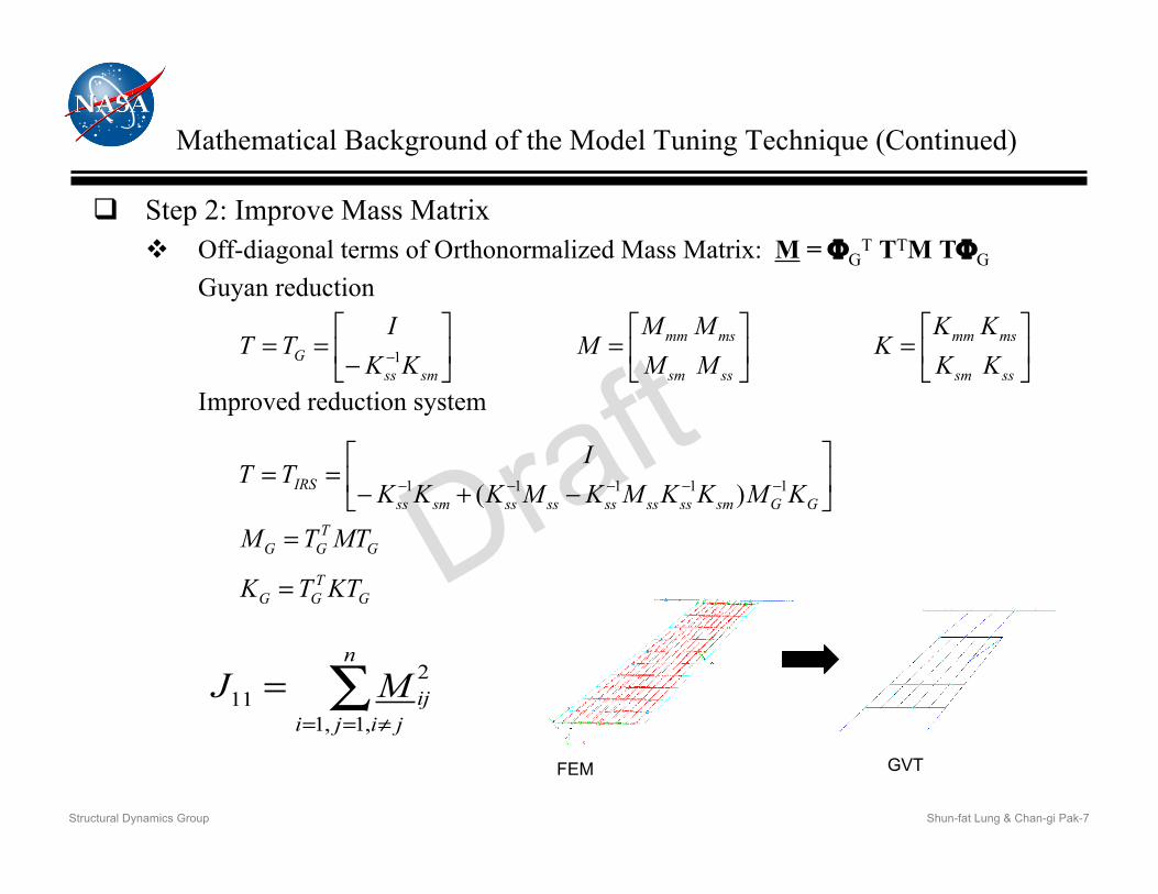
In the above equation the mass matrix, M, is calculated from the FE model, while the target eigen-matrix G! is measured from the GVT. The eigen-matrix G! remains constant during the optimization procedure. A transformation matrix T in the above equation is based on Guyan reduction [8] or improved reduction system [9]. This reduction is required due to the limited number of available sensor locations.

2.3 Frequencies and Mode Shapes Two different types of error norm can be

used. In the first option, the objective function considered combines an index which identifies normalized errors from the GVT and computed frequencies with another index which defines the total error associated with the off-diagonal terms of the orthonormalized stiffness matrix.

J12=

!i" !

iG

!i

#

$%&

'(i=1

n

)2

J13= K

ij( )i=1, j=1,i! j

n

"2

The matrix K are obtained from the following matrix products,

K = !

G

TTTKT!

G

where the stiffness matrix, K, is calculated from the FE model.

In the second option, the error norm combines the same index used above (which defines the normalized error in the GVT and computed frequencies) with another index which defines the total error between the GVT and computed mode shapes at given sensor points.

J12=

!i" !

iG

!i

#

$%&

'(i=1

n

)2

J13= !i " !iG( )

i=1, j=1,i# j

n

$2

In this research, the second optimization option is employed since the definition of the objective function is much simpler than in the first option. Any errors in both the modal frequencies and the mode shapes are minimized by including an index for each of these in the objective function. For this optimization, a small number of sensor locations can be used at which errors between the GVT and computed mode shapes are obtained. Any one of J1 thru J13 can be used as the objective function with the others treated as constraints. This gives the flexibility to achieve the particular optimization goal while maintaining the other properties at as close to the target value as possible. The optimization problem statement can be written as

Minimize: Ji Such that: Jk ! εk , for k = 1 thru 13 and k ! i

where εk is a small value which can be adjusted according to the tolerance of each constraint condition.

3 Applications

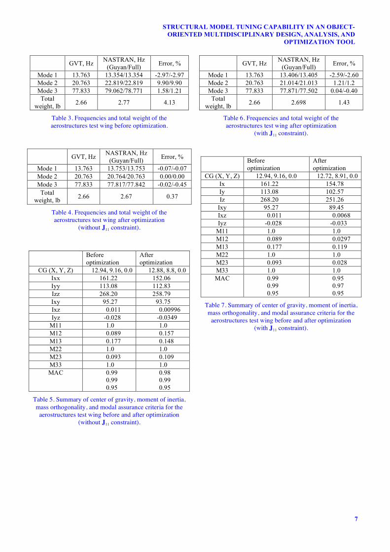
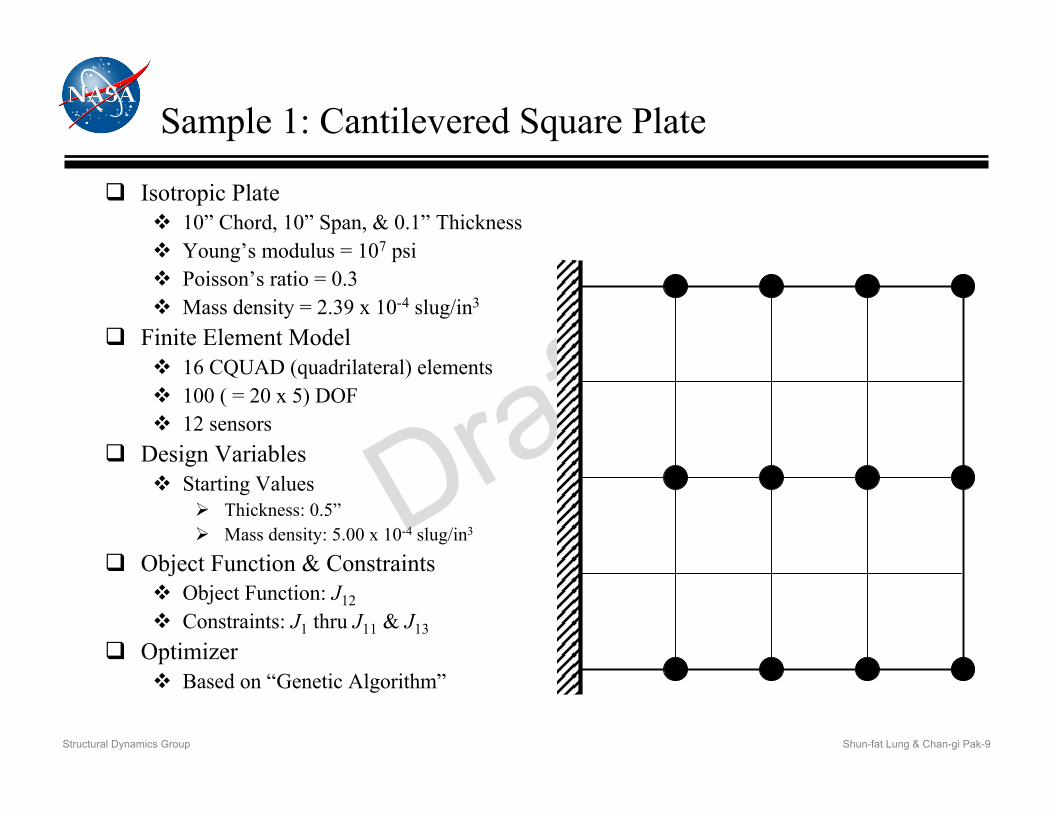
3.1 Square Cantilever Plate A cantilever plate shown in Fig. 1 is used

to demonstrate how to set up design variables, the objective function, and the constraints for the optimization process. The target configuration of the plate is 10 in. by 10 in. and 0.1 in. thick, containing 16 quadrilateral elements and 100 (20 × 5) degrees of freedom [DOFs]. Only 12 DOFs as shown in Fig.1 are used to simulate sensor output. The modulus of elasticity and Poisson’s ratio are 1.0 × 107 psi and 0.3, respectively. The mass density is 2.39 × 10-4 slug/in3.

The FE analysis results based on the target configuration are used as target values. The optimization process starts by selecting thickness and mass density to be the design variables. Total mass, CG, moment of inertia, and mass orthogonality are selected as constrained equations. Frequencies and mode shape errors are selected as the objective

5

STRUCTURAL MODEL TUNING CAPABILITY IN AN OBJECT-ORIENTED MULTIDISCIPLINARY DESIGN, ANALYSIS, AND

OPTIMIZATION TOOL

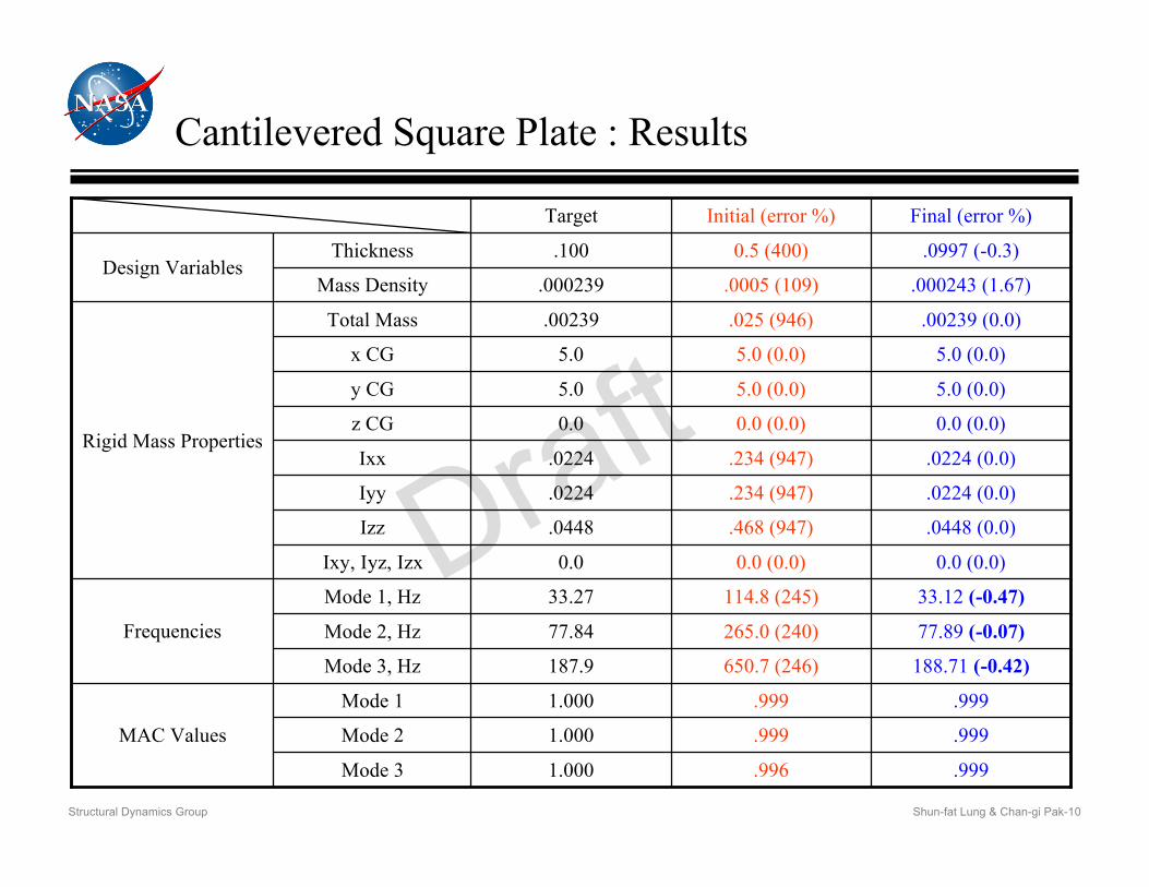
function. Initial design variables of 0.5 in. thick and a mass density of 5.0 × 10-4 slug/in3 are modeled such that a discrepancy between the two models is generated. Twenty populations and 100 generations are used for the genetic algorithm. Mass properties, modal characteristics, and design variables before and after optimizations are given in Tables 1 and 2. The thickness and mass density have converged to the target values and the frequencies and mode shapes have minimal errors. The optimization history of the objective function is shown in Fig. 2.

3.2 Aerostructures Test Wing A second example is an experiment known

as the aerostructures test wing [ATW] which was designed by NASA DFRC to research aeroelastic instabilities. Specifically, this experiment was used to study an instability known as flutter. Flight flutter testing is the process of determining a flight envelope within which an aircraft will not experience flutter. Flight flutter testing is very dangerous and expensive because predictions of the instability are often unreliable due to uncertainties in the structural dynamic and aerodynamic models.

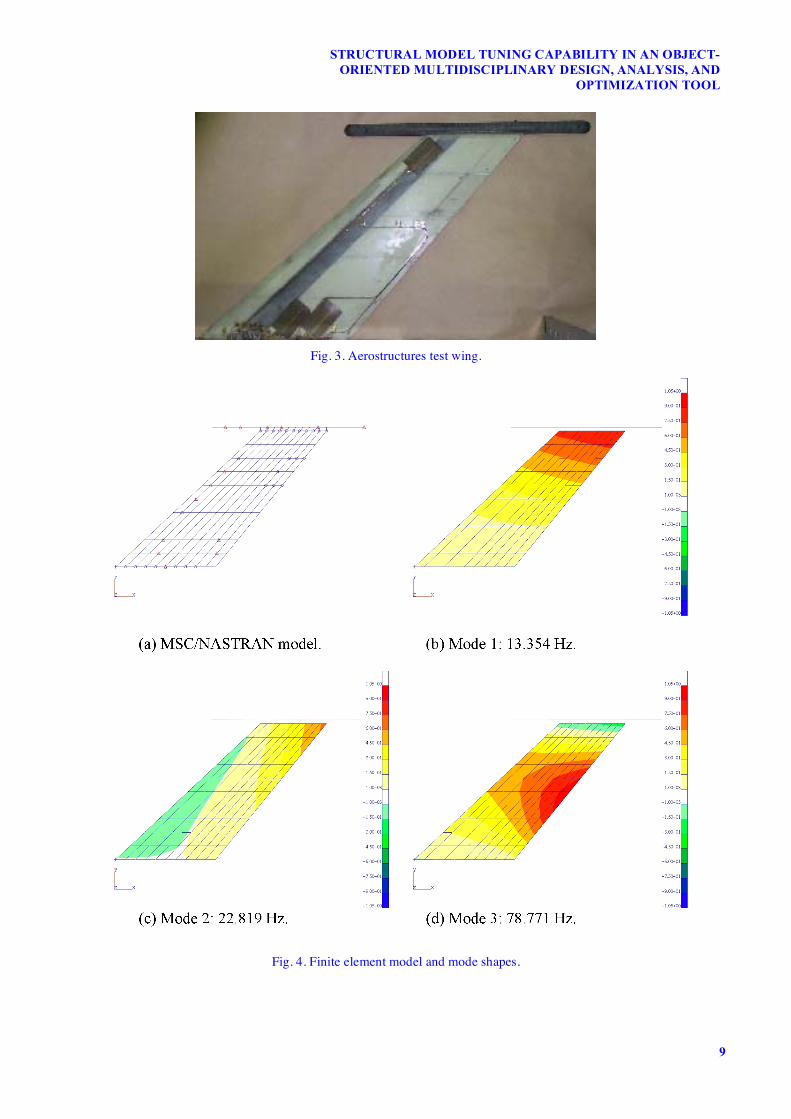
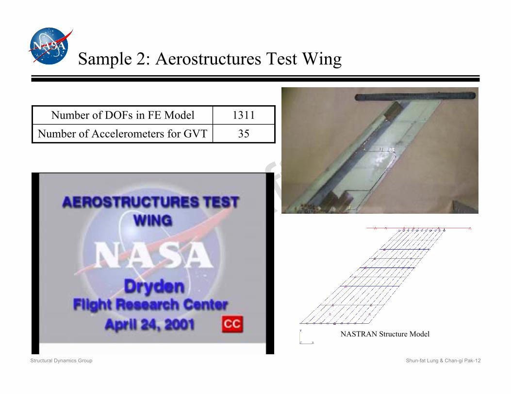
The ATW was a small-scale airplane wing comprised of an airfoil and wing tip boom as shown in Fig. 3. This wing was formulated based on a NACA-65A004 airfoil shape with a 3.28 aspect ratio. The wing had a span of 18 in. with root chord length of 13.2 in. and tip chord length of 8.7 in. The total area of this wing was 197 in2. The wing tip boom was a 1-in. diameter hollow tube of 21.5 in. length. The total weight of the wing was 2.66 lb.

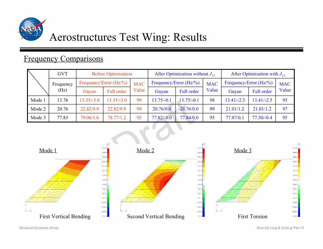
Ground vibration tests have been performed to determine the dynamic modal characteristics of the ATW [10]. It is shown in Table 3 that the first bending and torsion modes were at 13.76 and 20.76 Hz, respectively. Corresponding frequencies and mode shapes computed using MSC/NASTRAN (MSC.Software Corporation, Santa Ana, California, USA) [11] are also listed in Table 3 and given in Fig. 4, respectively.

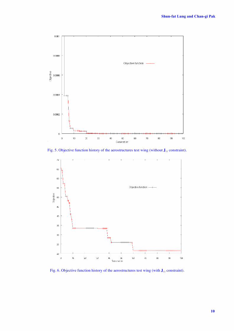
The FE model has been tuned to match the experimental data, but still the frequency error of 9.9% is observed for the second mode. This amount of frequency error violates the 3% limit for the primary modes described in military specifications [12, 13]. The 4% error in the total weight is also listed in Table 3. Therefore, the FE model needs to be further updated for a more reliable flutter analysis. The original FE model used rigid body elements to connect the wing tip to the boom which could produce the so-called ‘idealization error.’ Therefore, we used scalar springs to replace rigid body elements so that stiffness could be adjusted in this area. Point masses and scalar springs are selected for the design variables to minimize the frequencies and total weight errors. Two runs have been performed to demonstrate the sensitivity of the optimization solution to the constraint equations: (1) J12 was used as the objective function and J1 as a constraint equation; (2) J12 was used as the objective function and J1 thru J11 and J13 as constraint equations. With 50 populations and 100 generations of genetic algorithm optimization parameters, the final frequencies and total weight for case (1) are listed in Table 4. A summary of the center of gravity, moment of inertia, mass orthogonality, and MAC for the ATW for case (1) are shown in Table 5. Table 6 shows the final frequencies and total weight for case (2); a summary of the center of gravity, moment of inertia, mass orthogonality, and MAC are shown in Table 7. The optimization histories for the objective function of case (1) and case (2) are shown in Figs. 5 and 6 respectively. In case (1), there is a great reduction in the total weight and frequency errors but no improvement for the mass orthogonality. In case (2), total mass, mass orthogonality and frequencies are improved but not as much in case (1).

4 Conclusions Simple and efficient model tuning

capabilities based on a non-linear optimization problem are successfully integrated with the multidisciplinary design, analysis, and optimization [MDAO] tool developed at the NASA Dryden Flight Research Center. Instead of modifying the stiffness and mass matrices

Shun-fat Lung and Chan-gi Pak

6

directly, we updated the structural parameters such that the mass properties, mass matrix, frequencies, and mode shapes were matched to the target data, maintaining some similarity with the actual structure. The computer program has been coded in such a way that each J1 thru J13 can be used as a constraint or objective function. When Ji is selected as the objective function, all or part of the Jk ( k ! i ) can be selected as a set of constraints. This gives the flexibility to achieve a particular optimization goal.

Two examples were used to demonstrate the application of this model updating process. These examples showed that the number of constraint equations that is adequate to be used in the optimization process depends on the complexity of the model. For a simple model, the number of constraint equations may not have much effect on the solution, but for a complex model this effect could be significant. In either case, the approach investigated in this work proved to be a robust method of improving the accuracy of structural dynamics finite element models.

References [1] Friswell M and Mottershead J. Finite element model

updating in structural dynamics. Kluwer Academic Publishers, 1995.

[2] Mottershead J and Friswell M. Model updating in structural dynamics: a survey. Journal of Sound and Vibration, Vol. 16, No. 2, pp. 347-275, 1993.

[3] Pak C. Finite element model tuning using measured mass properties and ground vibration test data. VIB-07-1204, accepted for publication by ASME Journal of Vibration and Acoustics.

[4] Pak C and Li W. Multidisciplinary design, analysis, and optimization tool development using a genetic algorithm. To be presented at the 26th Congress of the International Council of the Aeronautical Sciences (ICAS), Anchorage, Alaska, 2008.

[5] Vanderplaats G. Numerical optimization techniques for engineering design. 3rd edition. Vanderplaats Research & Development, Inc., 2001.

[6] Charbonneau P and Knapp B. A User’s Guide to PIKAIA 1.0. National Center for Atmospheric Research, 1995.

[7] Yeniay, Ö. Penalty function methods for constrained optimization with genetic algorithms. Mathematical and Computational Applications, Vol. 10, No. 1, pp. 45-56, 2005.

[8] Guyan, R. Reduction of stiffness and mass matrices. AIAA Journal, Vol. 3, No. 2, pp. 380-380, 1965.

[9] O’Callahan J. A procedure for an improved reduced system (IRS) model. Proceedings of the 7th International Modal Analysis Conference, Las Vegas, Vol. 1, pp. 17-21, 1989.

[10] Voracek D, Reaves M, Horta L and Potter S. Ground and flight test structural excitation using piezoelectric actuators. AIAA-2002-1349, 43rd AIAA/ASME/ASCE/AHS/ASC Structures, Structural Dynamics, and Materials Conference, Denver, Colorado, Apr. 22-25, 2002.

[11] Reymond M. and Miller M. MSC/NASTRAN 2005 quick reference guide: Vol. 1, MSC.Software, Santa Ana, 2005.

[12] Military Standard. Test Requirements for Launch, Upper-Stage, and Space Vehicles. MIL-STD-1540C Section 6.2.10, Sept. 15, 1994.

[13] Norton W. Structures flight test handbook. FFTC-TIH-90-001, 1990.

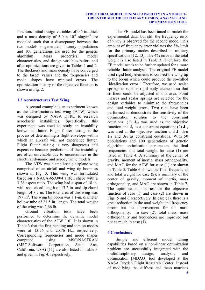
Tables

Target Initial Error, % Thickness 0.1 0.5 400.0 Mass density 0.000239 0.0005 109.2 Total mass 0.00239 0.025 946.0

CG 5.0, 5.0, 0.0 5.0, 5.0, 0.0 0 Ixx Iyy Izz

Ixy, Iyz, Izx

0.0224 0.0224 0.0448

0.0, 0.0, 0.0

0.234 0.234 0.468

0.0, 0.0, 0.0

944.6

Mode 1, Hz 33.27 114.84 245.2 Mode 2, Hz 77.84 265.00 240.4 Mode 3, Hz 187.91 650.70 246.3

Modal assurance

criteria

0.999 0.999 0.996

Table 1. Errors between the target and the initial configuration of the cantilever plate.

Target Final Error, %

Thickness 0.1 0.0977 -2.3 Mass density 0.000239 0.000236 -1.2 Total mass 0.00239 0.00231 -3.3

CG 5.0, 5.0, 0.0 5.0, 5.0, 0.0 0 Ixx Iyy Izz

Ixy, Iyz, Izx

0.0224 0.0224 0.0448

0.0, 0.0, 0.0

0.02162 0.02162 0.04320

0.0, 0.0, 0.0

-3.5

Mode 1, Hz 33.27 32.74 -1.6 Mode 2, Hz 77.84 77.01 -1.1 Mode 3, Hz 187.91 186.54 -0.7

Modal assurance

criteria

0.999 0.999 0.999

Table 2. Errors between the target and the final configuration of the cantilever plate.

7

STRUCTURAL MODEL TUNING CAPABILITY IN AN OBJECT-ORIENTED MULTIDISCIPLINARY DESIGN, ANALYSIS, AND

OPTIMIZATION TOOL

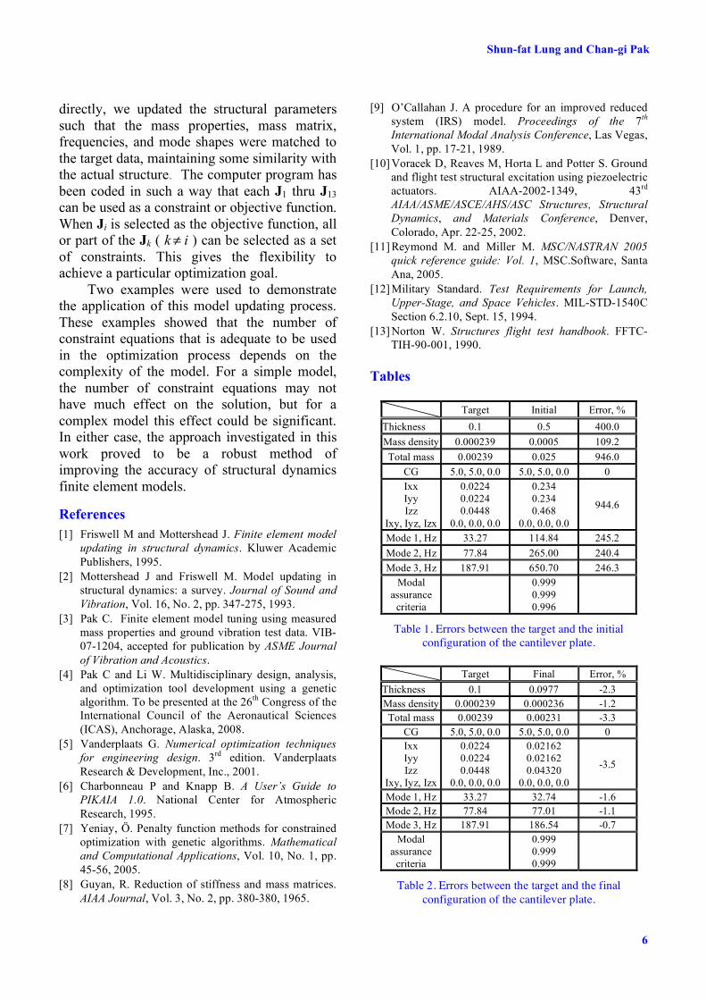
GVT, Hz NASTRAN, Hz (Guyan/Full) Error, %

Mode 1 13.763 13.354/13.354 -2.97/-2.97 Mode 2 20.763 22.819/22.819 9.90/9.90 Mode 3 77.833 79.062/78.771 1.58/1.21 Total

weight, lb 2.66 2.77 4.13

Table 3. Frequencies and total weight of the aerostructures test wing before optimization.

GVT, Hz NASTRAN, Hz (Guyan/Full) Error, %

Mode 1 13.763 13.753/13.753 -0.07/-0.07 Mode 2 20.763 20.764/20.763 0.00/0.00 Mode 3 77.833 77.817/77.842 -0.02/-0.45

Total weight, lb 2.66 2.67 0.37

Table 4. Frequencies and total weight of the aerostructures test wing after optimization

(without J11 constraint).

Before optimization

After optimization

CG (X, Y, Z) 12.94, 9.16, 0.0 12.88, 8.8, 0.0 Ixx 161.22 152.06 Iyy 113.08 112.83 Izz 268.20 258.79 Ixy 95.27 93.75 Ixz 0.011 0.00996 Iyz -0.028 -0.0349

M11 1.0 1.0 M12 0.089 0.157 M13 0.177 0.148 M22 1.0 1.0 M23 0.093 0.109 M33 1.0 1.0 MAC 0.99

0.99 0.95

0.98 0.99 0.95

Table 5. Summary of center of gravity, moment of inertia, mass orthogonality, and modal assurance criteria for the

aerostructures test wing before and after optimization (without J11 constraint).

GVT, Hz NASTRAN, Hz (Guyan/Full) Error, %

Mode 1 13.763 13.406/13.405 -2.59/-2.60 Mode 2 20.763 21.014/21.013 1.21/1.2 Mode 3 77.833 77.871/77.502 0.04/-0.40

Total weight, lb 2.66 2.698 1.43

Table 6. Frequencies and total weight of the aerostructures test wing after optimization

(with J11 constraint).

Before optimization

After optimization

CG (X, Y, Z) 12.94, 9.16, 0.0 12.72, 8.91, 0.0 Ix 161.22 154.78 Iy 113.08 102.57 Iz 268.20 251.26

Ixy 95.27 89.45 Ixz 0.011 0.0068 Iyz -0.028 -0.033

M11 1.0 1.0 M12 0.089 0.0297 M13 0.177 0.119 M22 1.0 1.0 M23 0.093 0.028 M33 1.0 1.0 MAC 0.99

0.99 0.95

0.95 0.97 0.95

Table 7. Summary of center of gravity, moment of inertia, mass orthogonality, and modal assurance criteria for the

aerostructures test wing before and after optimization (with J11 constraint).

Shun-fat Lung and Chan-gi Pak

8

Figures

Fig. 1. Cantilever plate.

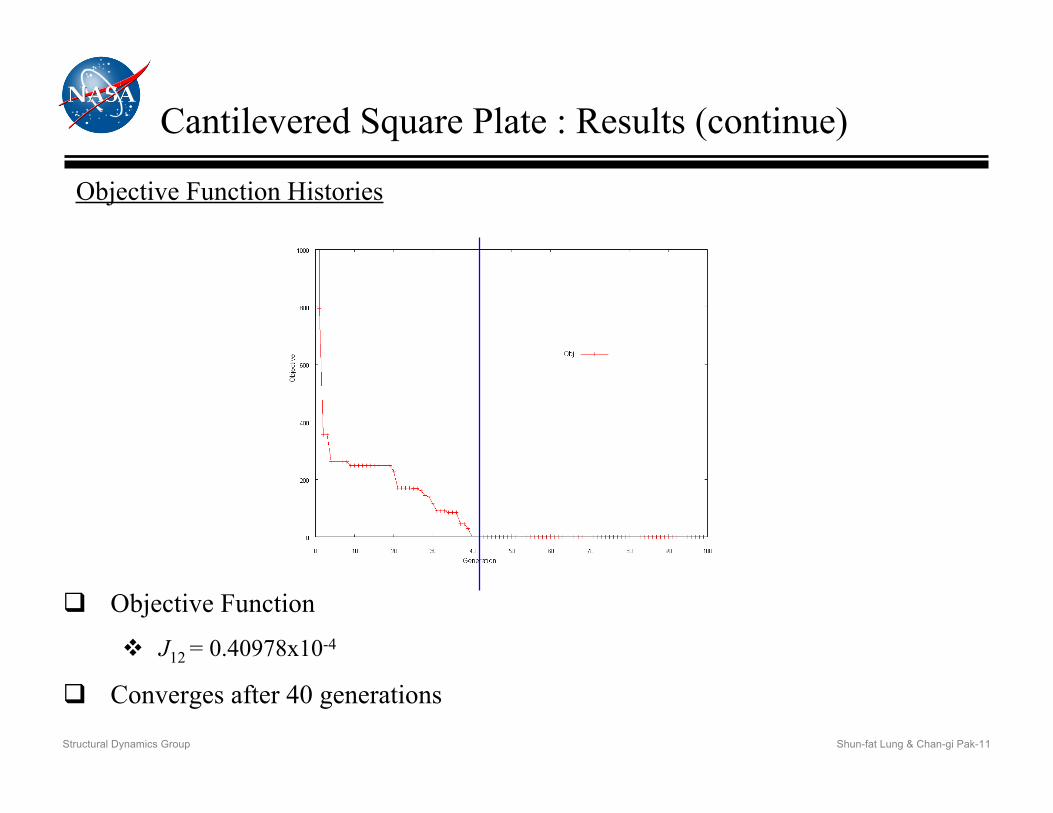
Fig. 2. Objective function history of the cantilever plate.

9

STRUCTURAL MODEL TUNING CAPABILITY IN AN OBJECT-ORIENTED MULTIDISCIPLINARY DESIGN, ANALYSIS, AND

OPTIMIZATION TOOL

Fig. 3. Aerostructures test wing.

Fig. 4. Finite element model and mode shapes.

Shun-fat Lung and Chan-gi Pak

10

Fig. 5. Objective function history of the aerostructures test wing (without J11 constraint).

Fig. 6. Objective function history of the aerostructures test wing (with J11 constraint).

11

STRUCTURAL MODEL TUNING CAPABILITY IN AN OBJECT-ORIENTED MULTIDISCIPLINARY DESIGN, ANALYSIS, AND

OPTIMIZATION TOOL

Copyright Statement The authors confirm that they, and/or their company or institution, hold copyright on all of the original material included in their paper. They also confirm they have obtained permission, from the copyright holder of any third party material included in their paper, to publish it as part of their paper. The authors grant full permission for the publication and distribution of their paper as part of the ICAS2008 proceedings or as individual off-prints from the proceedings.

Shun-fat Lung & Chan-gi Pak-1Structural Dynamics Group

Draft

Structural Model Tuning CapabilityStructural Model Tuning Capabilityin an Object-Oriented Multidisciplinaryin an Object-Oriented Multidisciplinary

Design, Analysis, and Optimization ToolDesign, Analysis, and Optimization Tool

Shun-fat Lung, Ph.D.* and Chan-gi Pak, Ph.D.**

Structural Dynamics GroupAerostructures Branch (Code RS)

NASA Dryden Flight Research Center

*: Presenter**: Group Leader

Shun-fat Lung & Chan-gi Pak-2Structural Dynamics Group

Draft

Objectives

To develop a simple and efficient in-house code forupdating finite element model using experimentaltest data

Be part of the MDAO tool development at NASADryden Flight Research Center

Support flight test by providing accurate flutterprediction based on reliable mass and stiffnessmatrices

Shun-fat Lung & Chan-gi Pak-3Structural Dynamics Group

Draft

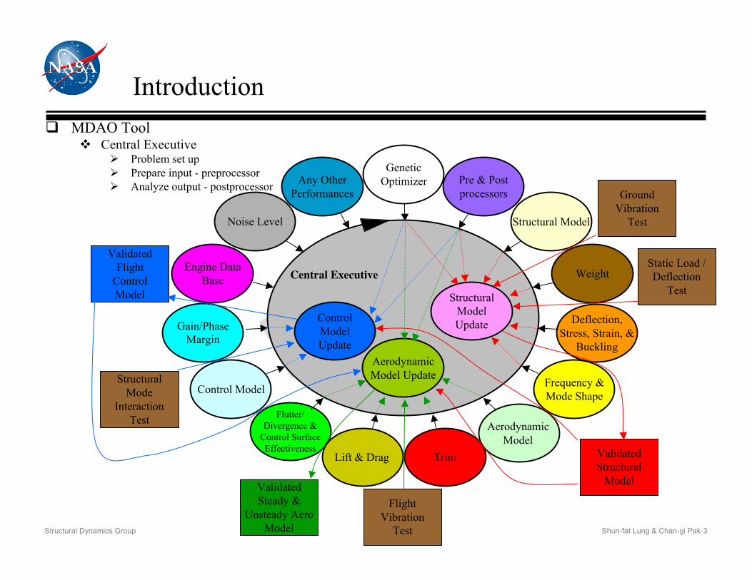
Introduction

Engine DataBase

Gain/PhaseMargin

Flutter/Divergence &

Control SurfaceEffectiveness

Frequency &Mode Shape

Deflection,Stress, Strain, &

Buckling

Weight

Pre & Postprocessors

Structural Model

AerodynamicModel

Trim

GeneticOptimizer

Control Model

Any OtherPerformances

Lift & Drag

Central Executive

Noise Level

StructuralModelUpdate

AerodynamicModel Update

ControlModelUpdate

Static Load /Deflection

Test

GroundVibration

Test

ValidatedStructural

Model

StructuralMode

InteractionTest

ValidatedFlight

ControlModel

ValidatedSteady &

Unsteady AeroModel

FlightVibration

Test

MDAO Tool Central Executive

Problem set up Prepare input - preprocessor Analyze output - postprocessor

Shun-fat Lung & Chan-gi Pak-4Structural Dynamics Group

Draft

Introduction (Cont.)

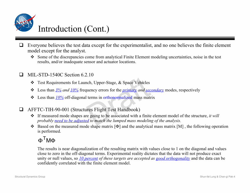
Everyone believes the test data except for the experimentalist, and no one believes the finite elementmodel except for the analyst. Some of the discrepancies come from analytical Finite Element modeling uncertainties, noise in the test

results, and/or inadequate sensor and actuator locations.

MIL-STD-1540C Section 6.2.10 Test Requirements for Launch, Upper-Stage, & Space Vehicles

Less than 3% and 10% frequency errors for the primary and secondary modes, respectively

Less than 10% off-diagonal terms in orthonormalized mass matrix

AFFTC-TIH-90-001 (Structures Flight Test Handbook) If measured mode shapes are going to be associated with a finite element model of the structure, it will

probably need to be adjusted to match the lumped mass modeling of the analysis. Based on the measured mode shape matrix [Φ] and the analytical mass matrix [M] , the following operation

is performed.

The results is near diagonalization of the resulting matrix with values close to 1 on the diagonal and valuesclose to zero in the off-diagonal terms. Experimental reality dictates that the data will not produce exactunity or null values, so 10 percent of these targets are accepted as good orthogonality and the data can beconfidently correlated with the finite element model.

!! MT

Shun-fat Lung & Chan-gi Pak-5Structural Dynamics Group

Draft

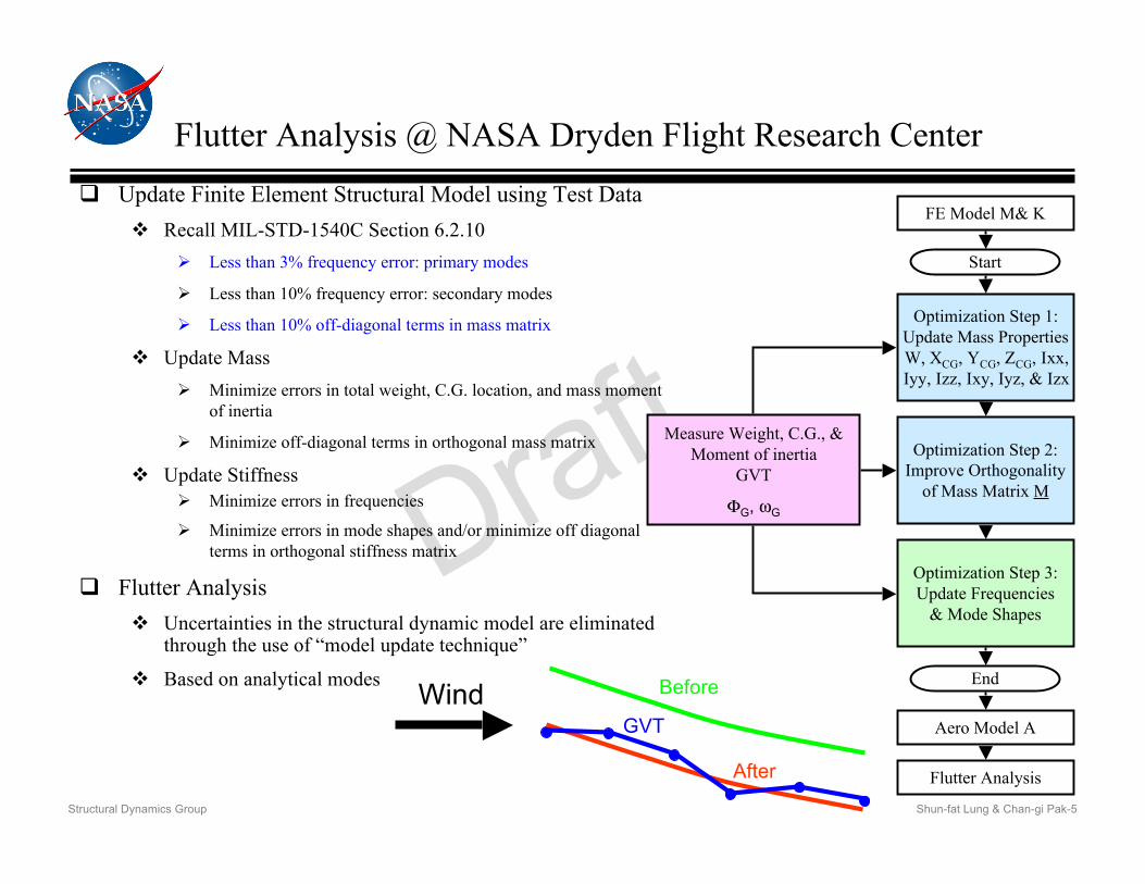
Flutter Analysis @ NASA Dryden Flight Research Center Update Finite Element Structural Model using Test Data

Recall MIL-STD-1540C Section 6.2.10 Less than 3% frequency error: primary modes

Less than 10% frequency error: secondary modes

Less than 10% off-diagonal terms in mass matrix

Update Mass Minimize errors in total weight, C.G. location, and mass moment

of inertia

Minimize off-diagonal terms in orthogonal mass matrix

Update Stiffness Minimize errors in frequencies

Minimize errors in mode shapes and/or minimize off diagonalterms in orthogonal stiffness matrix

Flutter Analysis Uncertainties in the structural dynamic model are eliminated

through the use of “model update technique”

Based on analytical modes

Measure Weight, C.G., &Moment of inertia

GVT

ΦG, ωG

WindGVT

Before

After

Optimization Step 1:Update Mass PropertiesW, XCG, YCG, ZCG, Ixx,Iyy, Izz, Ixy, Iyz, & Izx

End

Optimization Step 2:Improve Orthogonality

of Mass Matrix M

Optimization Step 3:Update Frequencies

& Mode Shapes

Start

Aero Model A

Flutter Analysis

FE Model M& K

Shun-fat Lung & Chan-gi Pak-6Structural Dynamics Group

Draft

Mathematical Background of the Model Tuning Technique

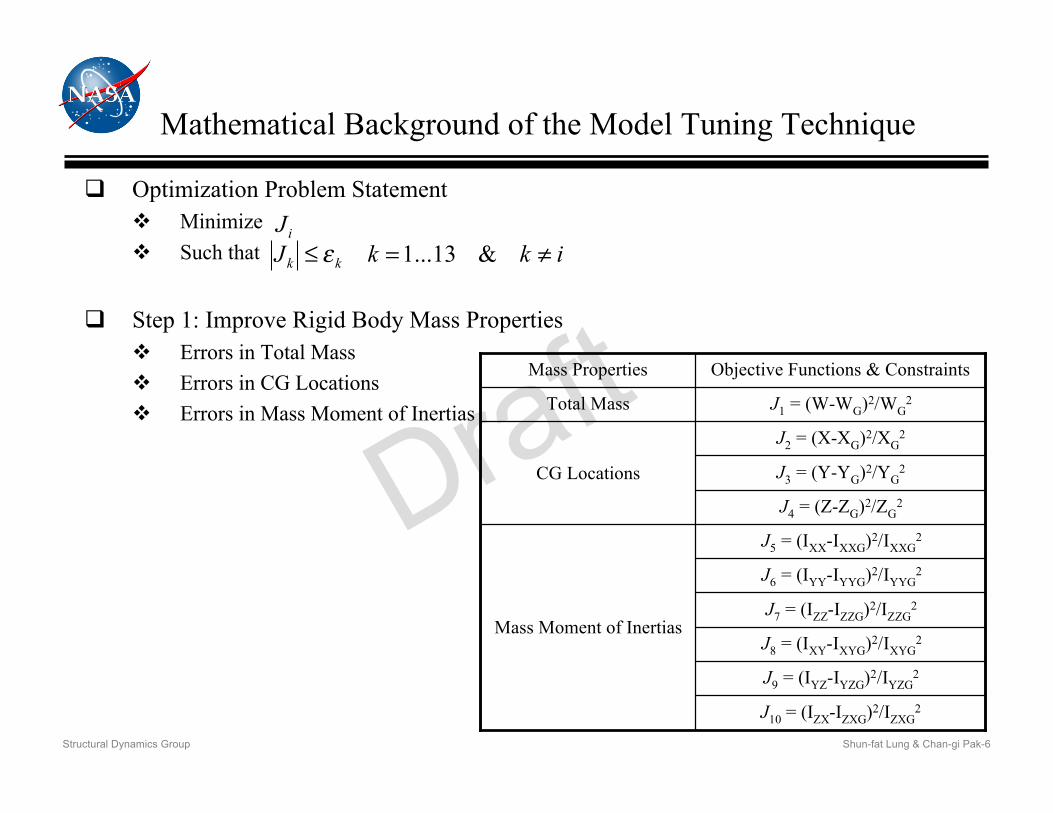
Optimization Problem Statement Minimize Such that

Step 1: Improve Rigid Body Mass Properties Errors in Total Mass Errors in CG Locations Errors in Mass Moment of Inertias

J10 = (IZX-IZXG)2/IZXG2

J9 = (IYZ-IYZG)2/IYZG2

J8 = (IXY-IXYG)2/IXYG2

J7 = (IZZ-IZZG)2/IZZG2

J6 = (IYY-IYYG)2/IYYG2

J5 = (IXX-IXXG)2/IXXG2

Mass Moment of Inertias

J4 = (Z-ZG)2/ZG2

J3 = (Y-YG)2/YG2

J2 = (X-XG)2/XG2

CG Locations

J1 = (W-WG)2/WG2Total Mass

Objective Functions & ConstraintsMass Properties

ikkJkk

!=" &13...1#

iJ

Shun-fat Lung & Chan-gi Pak-7Structural Dynamics Group

Draft

Mathematical Background of the Model Tuning Technique (Continued)

Step 2: Improve Mass Matrix Off-diagonal terms of Orthonormalized Mass Matrix: M = ΦG

T TTM TΦG

Guyan reduction

Improved reduction system

!"==

=

n

jiji

ijMJ,1,1

2

11

!"

#$%

&

'==

'smss

GKK

ITT

1

!"

#$%

&

'+'==

'''''GGsmsssssssssssmss

IRSKMKKMKMKKK

ITT

11111 )(

!"

#$%

&=

ss

ms

sm

mm

M

M

M

MM !

"

#$%

&=

ss

ms

sm

mm

K

K

K

KK

G

T

GGMTTM =

G

T

GGKTTK =

FEM GVT

Shun-fat Lung & Chan-gi Pak-8Structural Dynamics Group

Draft

Mathematical Background of the Model Tuning Technique (Continued)

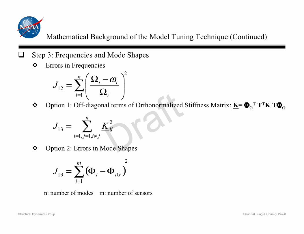
Step 3: Frequencies and Mode Shapes Errors in Frequencies

Option 1: Off-diagonal terms of Orthonormalized Stiffness Matrix: K= ΦGT TTK TΦG

Option 2: Errors in Mode Shapes

n: number of modes m: number of sensors

!=

""#

$%%&

'()(

=

n

i i

iiJ

1

2

12

*

( )2

1

13 !=

"#"=m

i

iGiJ

!"==

=

n

jiji

ijKJ,1,1

2

13

Shun-fat Lung & Chan-gi Pak-9Structural Dynamics Group

Draft

Sample 1: Cantilevered Square Plate

Isotropic Plate 10” Chord, 10” Span, & 0.1” Thickness Young’s modulus = 107 psi Poisson’s ratio = 0.3 Mass density = 2.39 x 10-4 slug/in3

Finite Element Model 16 CQUAD (quadrilateral) elements 100 ( = 20 x 5) DOF 12 sensors

Design Variables Starting Values

Thickness: 0.5” Mass density: 5.00 x 10-4 slug/in3

Object Function & Constraints Object Function: J12 Constraints: J1 thru J11 & J13

Optimizer Based on “Genetic Algorithm”

Shun-fat Lung & Chan-gi Pak-10Structural Dynamics Group

Draft

Cantilevered Square Plate : Results

.999.9961.000Mode 3

.999.9991.000Mode 2

.999.9991.000Mode 1

MAC Values

Frequencies

Rigid Mass Properties

Design Variables

0.0 (0.0)0.0 (0.0)0.0z CG

5.0 (0.0)5.0 (0.0)5.0y CG

188.71 (-0.42)650.7 (246)187.9Mode 3, Hz

77.89 (-0.07)265.0 (240)77.84Mode 2, Hz

33.12 (-0.47)114.8 (245)33.27Mode 1, Hz

0.0 (0.0)0.0 (0.0)0.0Ixy, Iyz, Izx

.0448 (0.0).468 (947).0448Izz

.0224 (0.0).234 (947).0224Iyy

.0224 (0.0).234 (947).0224Ixx

5.0 (0.0)5.0 (0.0)5.0x CG

.00239 (0.0).025 (946).00239Total Mass

.000243 (1.67).0005 (109).000239Mass Density

.0997 (-0.3)0.5 (400).100Thickness

Final (error %)Initial (error %)Target

Shun-fat Lung & Chan-gi Pak-11Structural Dynamics Group

Draft

Cantilevered Square Plate : Results (continue)

Objective Function

J12 = 0.40978x10-4

Converges after 40 generations

Objective Function Histories

Shun-fat Lung & Chan-gi Pak-12Structural Dynamics Group

Draft35Number of Accelerometers for GVT

1311Number of DOFs in FE Model

Sample 2: Aerostructures Test Wing

NASTRAN Structure Model

Shun-fat Lung & Chan-gi Pak-13Structural Dynamics Group

Draft 77.87/0.1

21.01/1.2

13.41/-2.5

Guyan

Frequency/Error (Hz/%)

After Optimization with J11

77.50/-0.4

21.01/1.2

13.41/-2.5

Full order

95

99

98

MACValue

78.77/1.2

22.82/9.9

13.35/-3.0

Full order Full orderGuyanGuyan

77.83

20.76

13.76

Frequency(Hz)

GVT

95

99

99

MACValue

9577.84/0.077.82/-0.079.06/1.6Mode 3

9720.76/0.020.76/0.022.82/9.9Mode 2

9513.75/-0.113.75/-0.113.35/-3.0Mode 1

MACValue

Frequency/Error (Hz/%)Frequency/Error (Hz/%)

After Optimization without J11Before Optimization

Aerostructures Test Wing: Results

Mode 3Mode 1 Mode 2

First TorsionFirst Vertical Bending Second Vertical Bending

Frequency Comparisons

Shun-fat Lung & Chan-gi Pak-14Structural Dynamics Group

Draft

Aerostructures Test Wing: Results (continue)

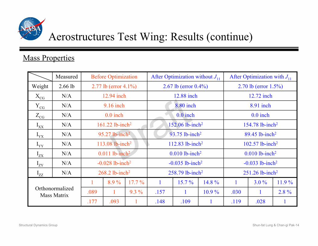
Mass Properties

.119

.030

1

251.26 lb-inch2

-0.033 lb-inch2

0.010 lb-inch2

102.57 lb-inch2

89.45 lb-inch2

154.78 lb-inch2

0.0 inch

8.91 inch

12.72 inch

2.70 lb (error 1.5%)

After Optimization with J11

.148

.157

1

258.79 lb-inch2

-0.035 lb-inch2

0.010 lb-inch2

112.83 lb-inch2

93.75 lb-inch2

152.06 lb-inch2

0.0 inch

8.80 inch

12.88 inch

2.67 lb (error 0.4%)

After Optimization without J11

.177

.089

1

268.2 lb-inch2

-0.028 lb-inch2

0.011 lb-inch2

113.08 lb-inch2

95.27 lb-inch2

161.22 lb-inch2

0.0 inch

9.16 inch

12.94 inch

2.77 lb (error 4.1%)

Before Optimization

N/A

N/A

N/A

N/A

N/A

N/A

N/A

N/A

N/A

2.66 lb

Measured

1.0281.1091.093

2.8 %110.9 %19.3 %1

11.9 %3.0 %14.8 %15.7 %17.7 %8.9 %Orthonormalized

Mass Matrix

IZZ

IZY

IZX

IYY

IYX

IXX

ZCG

YCG

XCG

Weight

Shun-fat Lung & Chan-gi Pak-15Structural Dynamics Group

Draft

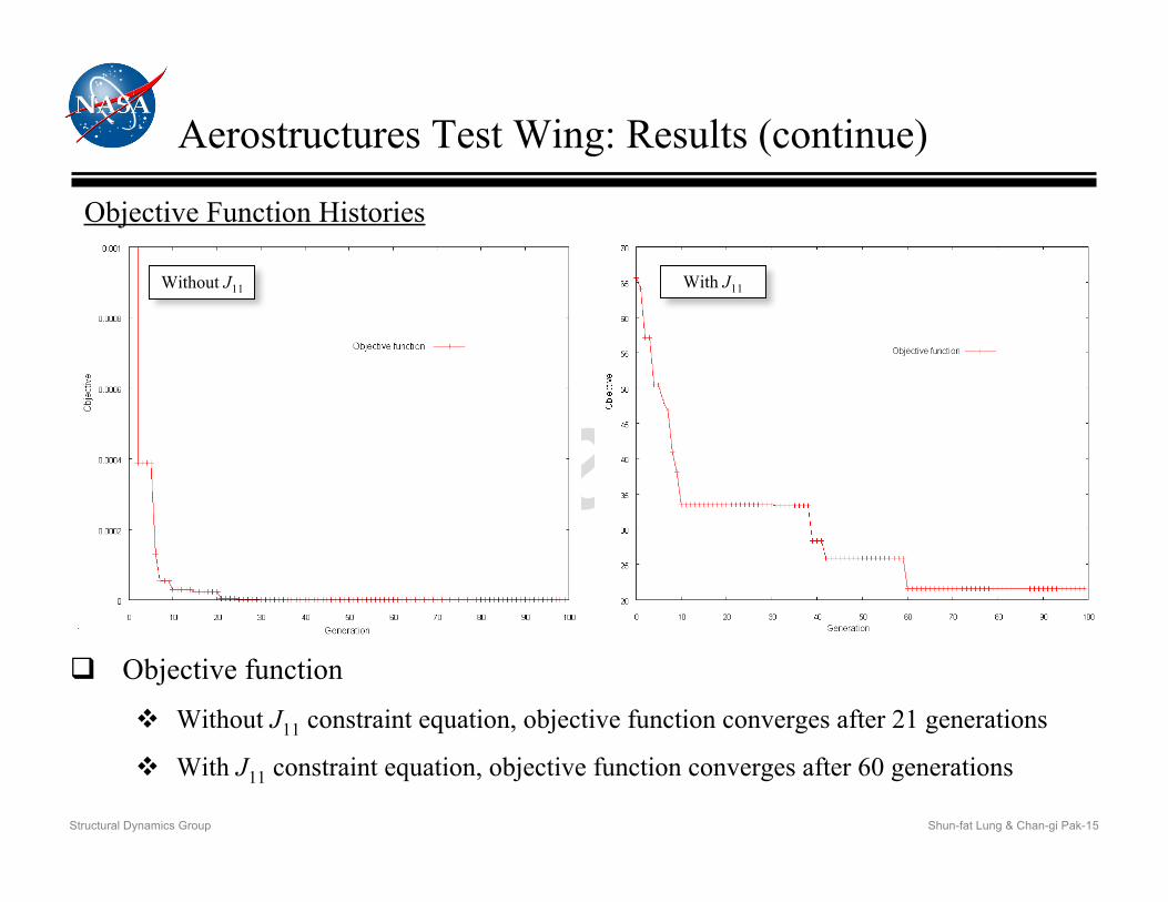
Aerostructures Test Wing: Results (continue)

Objective Function Histories

Without J11 With J11

Objective function

Without J11 constraint equation, objective function converges after 21 generations

With J11 constraint equation, objective function converges after 60 generations

Shun-fat Lung & Chan-gi Pak-16Structural Dynamics Group

Draft

Conclusions

Simple and efficient model tuning capabilities based on optimization problem aresuccessfully integrated with the MDAO tool developed at NASA Dryden Flight ResearchCenter. Structural properties are matched to the measured target data.

Mass properties, Orthonormalized mass & stiffness matrices, Frequencies, & mode shapes

Performance Indices: J1 through J13

If Ji is selected as objective function, then

All or part of Jk (k!i) can be selected as constraints.

Two examples are used to demonstrate the application of this model tuning process. Cantilever plate – Idealized problem

Use J12 as objective function

Use J1 thru J11, J13 as constraint equations

Aerostructures Test Wing – Practical problem Based on available experimental data

Use J12 as objective function

Use J1 and J13 as constraint equations.

Use J1, J11 and J13 as constraint equations

Shun-fat Lung & Chan-gi Pak-17Structural Dynamics Group

Draft

Questions ?