Structural Health Monitoring for Life Extension of Railway Bridges: Strategies and

Outcomes

Pradipta BANERJI* and Sanjay CHIKERMANE* * Department of Civil Engineering, Indian Institute of Technology Roorkee,

pbanerji.iitb@gmail.com

Abstract. Here the experience gained by the author and his co-researchers, in an association with the Indian Railways for over a decade, on the use of structural health monitoring strategies for establishing the current condition of steel railway bridges and an estimation of the remaining life of those bridges, is presented. Even in the case of bridges where the material used is either masonry or concrete, for which remaining life estimation is still a topic of research, it is shown that life extension can be done in a rational manner, based on the structural health monitoring outcomes and an estimation of future loading on the bridge. The various types of bridges encountered in this study account for approximately 99% of the more than 125,000 major bridges existing on the Indian Railway network. Only a few of the typical bridges will be detailed. The instrumentation and monitoring strategies adopted depend on the client’s requirement for the bridge, the form of the various bridge components, and a response and sensitivity analysis of preliminary numerical models that account for most of the significant behaviour expected of the bridge under the loading that it is currently being subjected. In some complicated cases, two preliminary numerical models with different basic assumptions have been considered. In almost all cases, the instrumentation scheme includes the requirement of estimation of current loads. Various outcomes have been studied too. These, of course depend on the type of the bridge, but also depend on the visual inspection of the state of bridge components during the monitoring program and the client’s requirements. Novel model updating and load estimation algorithms developed during the project are presented. These ensure that the current condition of the different bridge components can be estimated. The current condition of the bridge components, the current loads running on the bridge and the axle load spectrum and a projected traffic model are all important to study life extension of bridges, especially railway bridges. For steel bridges, the remaining life of the bridge and its components can be estimated conservatively based on established fatigue rules. For masonry and concrete bridges, the current condition of the bridge and current state of the material should be estimated, and then checks for future loads and their effects on the bridge and material can be done. The updated numerical models being subjected to future loads with design checks as per client’s specifications can be used as a rational basis for life extension of these bridges that are not made of steel. Damage detection algorithms developed during the project are also discussed, as they also have a large role to play in providing a rational basis for life extension. All of these points are illustrated using specific bridge examples.

Civil Structural Health Monitoring Workshop (CSHM-4) - Keynote 2

Licence: http://creativecommons.org/licenses/by-nd/3.0

1. Introduction

The problem of establishing the current condition of railway bridges and estimation of their remaining service life is a topic of current research. Subsequently, there have been significant issues related to the use of structures, mostly again bridges, beyond their design life, which has made structural health monitoring used specifically for current condition and remaining life assessment almost imperative as a bridge management tool (Yanev, 1998). Design life prediction of newly constructed bridges is obviously equally important (Li, et al, 2001 & Chan et al, 2001). For steel bridges that the estimation of remaining service life is usually done using a combination of measured stress histories, Miner’s rule (Miner, 1979), and railway codal fatigue curves (Chaminda, et al 2007). Even in the case of bridges where the material used is either masonry or concrete, for which remaining life estimation is still a topic of research, it is shown that life extension can be done in a rational manner, based on the structural health monitoring outcomes and an estimation of future loading on the bridge. (Banerji & Chikermane, 2011)

There are more than 125,000 major bridges – not considering culverts and minor bridges – on the Indian Railway network. A significantly large number of these are over 50 years old and some of them are close to being a century old. The trains plying these routes have been subject to several increases in the axle loads over this period and are now running loads far in excess of the standards existing during the construction and design of these bridges. In just recent times, over the last decade or so, the allowable axle loads were increased from 20.32 Tons axle load to 22.32 Tons and then to 22.82 Tons. It is now proposed that this loading is increased to 25 Tons axle loads, signifying an increase in loads of almost 25% in the last decade. This increase in axle loads permitted is also accompanied by a significant increase in the number of trains resulting in rapid increase in the total volume of traffic, computed in gross million tons, over the last decade (Banerji & Chikermane, 2011). In response to this increase of loading, Indian Railways launched an initiative to monitor and assess the condition of the bridges for suitability to this increased loading standards.

In this keynote paper, the experience gained by the author and his co-researchers, in this association with the Indian Railways for over a decade, on the use of structural health monitoring strategies for establishing the current condition of railway bridges of varying types is presented. The association with Indian Railways over this entire period generated a total work volume comprising more than 30 bridges of various span lengths – ranging from 6 meter span masonry arch bridges to 47.24 meter span open web steel girders. Various types of bridges including steel plate girders, open-web steel girders of both through and under-slung forms, composite RC slab-steel girders, pre-stressed concrete box girders and stone masonry arches were studied in this period. The substructures encountered were also of varying types – stone and brick masonry gravity piers, mass concrete piers, RC piers of various shapes and hollow steel piers with mass concrete infill. It is estimated that the various types of bridges in this study account for approximately 99% of the major bridge stock of the Indian Railway network.

Instrumentation and monitoring strategies were, almost in all cases, fine-tuned to incorporate the client’s needs and requirements, the form of bridge components and a detailed response and sensitivity analysis using preliminary numerical models – in some cases where structures were complicated, two preliminary models were used – to account for most of the significant behavior patterns expected from the bridge under the currently subjected service loading. In almost all of the cases considered, estimation of dynamic augment, longitudinal load estimations and estimation of current service loads plying on the track were client requisites.

The outcomes and responses were also variable, depending upon similar parameters as listed above. One significant additional parameter for the outcome was the visual inspection of the state of bridge components prior to the monitoring program. Novel model updating and load estimation algorithms were developed in the course of the study as a response to the requirements. Using these algorithms, the current condition of the bridge components was accurately and efficiently estimated. Damage detection algorithms were also developed during this study. These have a vital role to play in a rational basis for life extension of old structures. Specific bridge examples have been used in this work to illustrate the points discussed above.

2. Overview Of Bridges Studied

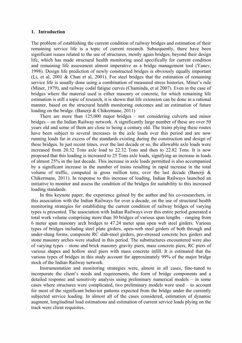
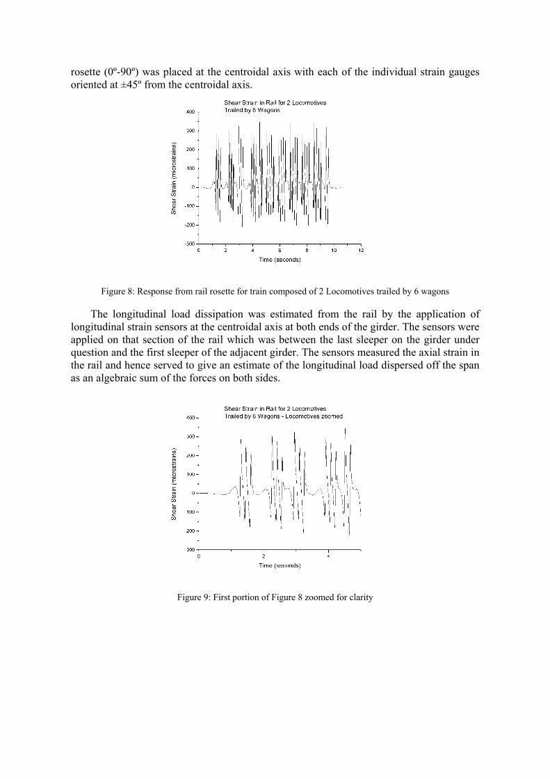
Large spectrums of bridges were considered for monitoring and analysis. These included open-web girders, plate girders, masonry arches, composite girders and pre-stressed concrete girders. The type distribution of the bridges studied is shown in Figure 1 and the span distribution in Figure 2. Except for the two multi-span masonry arches, all other bridges were simply supported and hence one or two spans could be considered as being representative of the entire bridge. For the present study, for all the bridges under consideration, only one span was instrumented and monitored. The results and findings for that span were then considered as being representative for the entire bridge. The simply supported bridges under consideration had various types of bearings ranging from rocker-roller bearings for open-web and composite girders, sliding and centralized bearings for the plate girders and elastomeric bearings for the pre-stressed concrete girders. Some of the representative bridges are shown in Figures 3 – 7. In this paper further, the results and analysis will be shown for some representative open-web girders, plate girders and masonry arches. The analysis and results for the composite girders and pre-stressed concrete girders are not considered in the scope of this paper.

Figure 1: Distribution of Bridges by Type

Figure 2: Distribution of Bridges by Span

Figure 3: Photograph of a typical 48 meter span open web through girder

Figure 4: Photograph of a typical 32 meter span Plate Girder

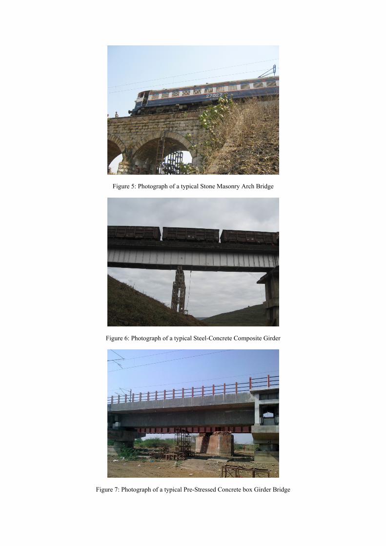
Figure 5: Photograph of a typical Stone Masonry Arch Bridge

Figure 6: Photograph of a typical Steel-Concrete Composite Girder

Figure 7: Photograph of a typical Pre-Stressed Concrete box Girder Bridge

3. Representative Instrumentation Schemes

There were several defined objectives defined by the Railway authorities for the work initiated. Some of the major objectives are listed below

1. To create a realistic numerical model of the bridge which accurately represents current conditions to enable simulations of different loading and operational conditions

2. To estimate the loads running on the girders and to arrive at a rational estimate of remaining service life of these girders

3. To estimate the longitudinal forces transmitted to the girders due to service conditions and to validate the structures for these loads

4. To estimate the effects of dynamic augment on the bridge components with a view to possibly restricting speeds on certain critical bridges

The instrumentation scheme was generated to address the defined objectives, and critical locations were identified which would give sufficient and clear information. For most of the structures, a preliminary analysis model is used to estimate the significant structural actions expected in a bridge. The instrumentation scheme is designed to either validate these actions or to generate a set of reference data against which the analysis model needs to be tuned to create a representative numerical model of the bridge, thus addressing the first of the listed objectives.

Representative instrumentation schemes for some different bridge types are described here. The displacement sensors used are linear potentiometers, the strain sensors are electrical resistance strain gauges of different gauge lengths – 5 mm gauge length for application on steel surfaces and 120 mm gauge length for application on concrete or masonry – which are bonded to the surface using the prescribed adhesives and the accelerometers used are of piezo-electric type. The data is collected using a dedicated data acquisition system which is capable of sampling the data at the necessary rate for civil engineering applications. The maximum sampling rate (including multiplexing) is in excess of 3200 Hz. For most of the current application the sampling is kept at 200 Hz, which has a Nyquist frequency of 100 Hz and is adequate for civil engineering applications.

3.1. Rail Instrumentation

The objectives of the rail instrumentation was three-fold – one was to estimate the dynamic augment due to speed of train movement at the rail level, second was to estimate the dissipation of the longitudinal forces through the rail-track system and the third was to generate the necessary information needed of the spatial distribution of the loads and the exact measured speed of travel. The third objective is critical for the estimation of loads, the results of which are not being presented in this paper as they have been submitted for publication elsewhere.

The rail track in almost all the bridges instrumented comprised a sleeper system of either pre-stressed concrete sleepers or steel channel sleepers at a spacing of about 0.6 meters on which the rail was placed. The dynamic impact was estimated by first identifying a location which would give a response due to each axle without any “smearing” of information from other axles. It was noted that the minimum distance between train axles was about 1.7 meters, which is significantly longer than the sleeper spacing, making the location of the rail between sleepers ideal for estimation of shear strains. It was found that these shear strains measured gave the presence of each axle clearly as a well-defined peak without any “smearing” of data from other axles as is shown in Figures 8 and 9. A strain

rosette (0º-90º) was placed at the centroidal axis with each of the individual strain gauges oriented at ±45º from the centroidal axis.

Figure 8: Response from rail rosette for train composed of 2 Locomotives trailed by 6 wagons

The longitudinal load dissipation was estimated from the rail by the application of longitudinal strain sensors at the centroidal axis at both ends of the girder. The sensors were applied on that section of the rail which was between the last sleeper on the girder under question and the first sleeper of the adjacent girder. The sensors measured the axial strain in the rail and hence served to give an estimate of the longitudinal load dispersed off the span as an algebraic sum of the forces on both sides.

Figure 9: First portion of Figure 8 zoomed for clarity

3.2. Super-Structure Instrumentation

3.2.1. Open-web girders

Vertical displacement at center of span is one of the most robust parameters and this is modeled in all open-web girders. In open-web girders, the significant strain actions are expected to be axial strains, and the instrumentation scheme reflects this. The instrumentation scheme, for open-web girders, is also designed to estimate the bending strains in members, which though being an order of magnitude lower than the axial strains, are expected to be more sensitive to local system changes and can be used as damage sensitive parameters. The instrumentation scheme incorporates a redundancy as corresponding members on both girders are instrumented. The bearing movements give an estimate of the degree of fixity in the bearing and are used for updating the numerical model boundary conditions. The accelerometers placed at middle and quarter spans are used to estimate the dynamic parameters of the model. The instrumentation scheme for a typical open-web girder is shown in figure 10. In addition to the scheme showed – for the main truss members – the cross girder and the stringer beams are identified as fatigue sensitive members from the preliminary analysis. This is due to their behavior pattern which essentially undergoes a loading-unloading cycle for each axle as against the main girder members which do this pattern for a full train. A fully loaded goods train plying this route has about 250 axles and hence the number of stress cycles for the floor members can be significantly higher than for the main truss members. These members are thus monitored to estimate their fatigue suitability.

For open web girders, the out of balance horizontal force at the first portal end-raker – bottom chord connection, gives a measure of the horizontal force transmitted through the super-structure. These members are shown in Figure 10 as L0-U1 & L0-L1 on the upstream side and L0’-U1’ & L0’-L1’ on the downstream side.

Figure 10: Instrumentation Scheme for Typical Open-web Through Girder

3.2.2. Plate Girder

Vertical displacement at center of span is monitored for all plate girders as well. In open-web girders, the significant strain actions are expected to be longitudinal strains at the extremities of the flanges at the center of span and the shear strain in the webs close to the end of span, and the instrumentation scheme reflects this. The instrumentation scheme incorporates a redundancy as corresponding locations on both girders are instrumented. The bearing movements give an estimate of the degree of fixity in the bearing and are used for updating the numerical model boundary conditions. The accelerometers placed at middle and quarter spans are used to estimate the dynamic parameters of the model. The instrumentation scheme for a typical plate girder is shown in figure 11.

Figure 11: Instrumentation Scheme for Typical Plate Girder

3.2.3. Masonry Arch

Figure 12: Instrumentation Scheme for Stone Masonry Arch (Banerji & Chikermane, 2012)

In stone Masonry Arches, the approach followed is that in addition to the displacements conventionally monitored by most researchers, the approach followed is to monitor the strain on the voussoir blocks as well. The displacements and the strains in the masonry arch are monitored as per the instrumentation scheme, shown in Figure 12, given by the authors (Banerji & Chikermane, 2012). It is shown here that if the modeling ideology is also changed from the conventional smeared model to a combination discrete-finite element model, there is excellent agreement between the monitored results and the predicted results from the updated numerical model.

3.3. Bearings

The two types of bearings commonly found in Indian Railway bridges were rocker bearings and sliding bearings (Figure 13 and Figure 14). For rocker bearings, the ribs in the main span direction were strain-gauged as it was estimated after a preliminary analysis that this parameter showed a significant effect of the horizontal force coming on the bearing. To avoid boundary effects, these sensors were placed at the slant mid-point as shown in Figure 13.

For sliding bearings, the first plate on which the girder rested was considered as being in uniform shear and a rosette was applied on this, as shown in Figure 14, to estimate the shear strain and hence the force. When sliding bearings are used in a bridge, they are typically used on both ends and the longitudinal force estimated is the algebraic addition of the forces estimated on both ends.

Figure 13: Rocker Bearings with applied strain gauges

3.4. Sub-Structure

The sub-structure was also instrumented at the base (just above the ground level) to estimate the strains in the piers and abutments. The piers were strain-gauged on three faces, the face just below the span, the face opposite to the span and one of the side faces. The side face being on the neutral bending axis for in-plane bending of the pier, correspond to the axial strain, while the faces in direction of the span would give combined effects due to axial and bending actions. From these strains, estimate of the longitudinal loads are worked out at the sub-structure levels.

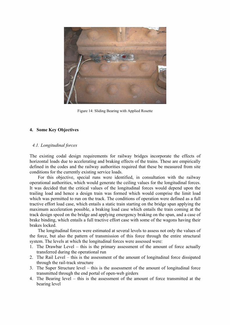
Figure 14: Sliding Bearing with Applied Rosette

4. Some Key Objectives

4.1. Longitudinal forces

The existing codal design requirements for railway bridges incorporate the effects of horizontal loads due to accelerating and braking effects of the trains. These are empirically defined in the codes and the railway authorities required that these be measured from site conditions for the currently existing service loads.

For this objective, special runs were identified, in consultation with the railway operational authorities, which would generate the ceiling values for the longitudinal forces. It was decided that the critical values of the longitudinal forces would depend upon the trailing load and hence a design train was formed which would comprise the limit load which was permitted to run on the track. The conditions of operation were defined as a full tractive effort load case, which entails a static train starting on the bridge span applying the maximum acceleration possible, a braking load case which entails the train coming at the track design speed on the bridge and applying emergency braking on the span, and a case of brake binding, which entails a full tractive effort case with some of the wagons having their brakes locked.

The longitudinal forces were estimated at several levels to assess not only the values of the force, but also the pattern of transmission of this force through the entire structural system. The levels at which the longitudinal forces were assessed were: 1. The Drawbar Level – this is the primary assessment of the amount of force actually

transferred during the operational run 2. The Rail Level – this is the assessment of the amount of longitudinal force dissipated

through the rail-track structure 3. The Super Structure level – this is the assessment of the amount of longitudinal force

transmitted through the end portal of open-web girders 4. The Bearing level – this is the assessment of the amount of force transmitted at the

bearing level

4.2. Dynamic Augment

The current codal design requirements specify a significant augmentation of loads to account for the expected increase in response due to speed effects. Current practices are also to impose speed restrictions on girders which are found to be border-line in order to lower the effects of augmentation. It was required to estimate these effects on different bridge components as part of the overall project scope.

This was addressed by defining a specific train as described above and running it on the span at different speeds up to and including the design track speed of the bridge section. The augments were then computed based upon the peak values of responses seen at each sensor location. At the rail level, the rail giving a well-defined peak for each axle, the value of the augment was worked out for each individual axle and the overall augment for the speed worked out as an average of these values.

4.3. Other Objectives influencing instrumentation schemes

The load estimation objective was addressed in the instrumentation scheme by using, other than the critical locations giving significant response values, by application of place-holder sensors which gave an accurate representation of the axles of the train – thus enabling an accurate estimation of both the spatial representation of the loads and the speed of the train. The graphs of these sensors are shown in Figure 8 & 9. The placing of these sensors at a pre-defined distance apart enabled an accurate computation of the velocity based upon the time lag between each peak. This value was computed for each axle and signified the entry velocity of the train on the span. Similarly the spatial configuration of the axles was also estimated. This gave an accurate estimation of the train for computing the loads. The complete load estimation procedure has been submitted elsewhere for publication and hence its details are not being mentioned here.

5. Modeling Strategies

Numerical modeling strategies were customized based upon the type of bridge being modeled. A combination of finite and discrete element techniques were used for the different types of bridges based upon an engineering expectation of their behavior patterns. For steel bridges, the material model is taken as a linear isotropic model with Young’s modulus and Poisson’s ratio based upon testing of actual samples from the bridges considered. A short description of the modeling strategies used for the different types of bridges is described here.

5.1. Open-Web Girders

Although the Indian railway codes design open web girders as pure trusses, the behavior of the bridge showed that there were some amounts of bending strains coming on the main girder members due to train loads. Although the elements were seen to be predominantly axial, for increased accuracy in modeling, the elements were modeled as beam elements with the connection between members being modeled based upon site conditions. The bottom and top chords, since they are actually continuous members were modeled as such, and the other chords were connected to these using rotational springs, the stiffness of which could be changed during the model updating procedure to converge the response values. The members were meshed using 20 elements per member to capture the in-plane and out-

of-plane bending modes for these members. The boundary conditions for these members were modeled as being a pin on one end – the rocker end – and a roller with a longitudinal fixity on the other end to model a non-ideal roller condition. The fixity in the numerical model took the form of a linear spring element which was updated to reflect the site measured recording. Physical offsets as exist based upon site geometric conditions were modeled.

5.2. Plate Girders

There were two different modeling strategies adopted for the plate girder bridges. In the first strategy, the bridge was modeled as a beam with the necessary offsets at the ends. In this procedure, the cross bracings and diagonal bracings were not modeled, but their effect was considered by assuming that they give sufficient lateral stability and hence a single beam was modeled. The loads were assumed to be perfectly balanced laterally and half the axle load was modeled as a moving load on the beam. The boundary conditions were modeled using linear spring elements and adjusting their stiffness to get a corroborating fit with the site measured boundary conditions. A representative model using this ideology is shown in Figure 15.

Figure 15: Schematic Representation of a beam model for plate girders

Another modeling ideology adopted for these girders was using shell elements with appropriate thickness as measured from site conditions. The bracings and stiffeners were modeled as beam elements overlaid on the shell, sharing the same nodes at connection points. The interface between the beams and shells was considered as a perfect connection. The boundary conditions on both ends were modeled as a roller connection with an additional longitudinal fixity in the form of a spring to account for fixities as would exist on site. These were updated based upon site data recordings. A representative model is shown in Figure 16.

Figure 16: Finite element representation of a shell-beam model for plate girders

5.3. Masonry Arch

The exact methodology of modeling the masonry arch is presented in Banerji & Chikermane (2012). The modeling ideology considered is a plane strain approach. The stone voussoirs are modeled using a linear isotropic material as they are not expected to undergo any non-linearity in the stress ranges they are subject to. The mortar is modeled as a non-linear spring element with a very small tensile lift off value – necessary for convergence – which, however, resists shear up to a pre-defined limit after which a snap-through failure can occur. The fill is modeled as a Drucker-Prager element and the heterogeneity of fill is considered as it is expected to have different densities at different locations. The fill-masonry interface is modeled using a series of contact elements which resist sliding. The numerical model of the arch is shown in Figure 17 & 18. Geometrically the arch is modeled exactly as exists in site conditions based upon individual voussoir measurements. The material parameters are modeled as variables which are updated using a multiple-pass updating procedure as described in Banerji & Chikermane (2012) within ranges based upon an engineering judgment.

Figure 17: Finite-Discrete element model of arch bridge (Banerji & Chikermane, 2012)

Figure 18: Blown up model of arch bridge for clarity (Banerji & Chikermane, 2012)

6. Analysis Of Outcomes

Post instrumentation, for most of the bridges under consideration, a “design train” was formed on site. This train comprised a configuration of locomotives followed by a set of wagons having known pre-measured axle loads. The rear of the train was again comprised of a configuration of locomotives to enable smooth running in both directions. This train hence comprised a known set of loads imposed upon the girder. The overall set of runs done comprised all the possible extreme load based events that the bridge could be subject to including traction and braking runs. There were also several constant velocity runs done on the girder with velocities varying from crawling speed to the track design speed for the track section in which the girder fell. Based upon this reference data, it was attempted to first create a representative numerical model that represented the performance and behavior of the actual girder under question, and then use this model to generate several simulated load conditions on the girder corresponding to the proposed change in load conditions and spectrum.

6.1. Model updating for steel girders

The model updating for steel open-web girders is done in three stages. Each of these stages gives certain incremental information about the condition of the girder. This is possible because over the spectrum of steel girders analyzed it is generally seen that the response parameters can be divided into three disjoint non-intersecting sets. These comprise firstly the global major response parameters like the vertical displacements and axial strains in the main truss members of an open web girder bridge which primarily depend upon the gross member cross sectional properties, the material model and boundary conditions. Some examples of the updating of boundary conditions are shown in Figures 19 – 20 and the convergence of axial strains in Figures 21 – 22.

Secondly the primary bending strains which fundamentally depend upon the joint connectivity between members as shown in Figures 23 – 24, and finally the out-of-plane strains and the local frequencies where the member behaves as a part of a sub-structure within the entire global structure which depend upon the out-of-plane connectivity properties. Details of this last set are not given as they are pending publication. A sensitivity analysis establishes the primary disjoint nature of these three parameter sets. The three different updating levels are used for making different conclusions of the condition of the structure.

The primary updating serves to give the overall condition of the girder and creates a model which accurately estimates the major response parameters. This model can be used for most of the simulation approaches as the major design parameters comprise the primary responses. The secondary updating generates models which are used for more accurate analysis processes such as load estimations and other inverse problems. This is because inverse problems are very sensitive to the small fluctuations induced due to non-convergence of the secondary response parameters. The tertiary updating is needed for damage detection as global parameters are virtually insensitive to the kind of damage expected in bridges of this nature.

Figure 19: Comparisons for Vertical Displacement at Centre Span – Underslung Girder

Figure 20: Comparisons for Bearing Displacement – Underslung Girder

Figure 21: Comparisons for Top Chord Axial Strain at Centre Span – Underslung Girder

Figure 22: Comparisons for Top Chord Axial Strain at Rocker End – Underslung Girder

Figure 23: Comparisons for Top Chord bending Strain at Centre Span – Underslung Girder

Figure 24: Comparisons for Top Chord Bending strain at Rocker end – Underslung Girder

6.2. Dynamic Parameter Estimation

The dynamic parameters were extracted from the converged numerical model and compared with the parameters from the raw data to validate convergence. Several algorithms such as Peak picking, frequency domain decomposition, eigenvalue realization algorithm and stochastic subspace algorithms were used to extract dynamic parameters from raw data (Banerji & Chikermane 2009a & 2009b).

The estimation algorithms were fundamentally divided into frequency domain methods and time domain methods. Frequency domain methods work by fundamentally identifying the frequency directly, whereas time domain methods first estimate the system matrices and then estimate the frequency through decomposition of the system matrices. Most frequency domain methods are variants of the classical peak picking method, the results of which are shown in Figure 25. The compiled results are shown in Table 1.

Figure 25: Typical Frequency Spectrum

Table 1: Compiled results for Frequency Estimation

Mode

Peak Picking

(Hz)

Frequency Domain

Decomposition

(Hz)

ERA (Hz)

Stochastic Subspace

(Hz)

Averaged Values (Hz)

Converged Numerical Model (Hz)

1 4.29 3.52 3.83 4.58 4.06 4.20

6.49 6.64 6.57

2 7.23 7.42 7.11 7.94 7.43 7.64

3 9.82 9.77 9.96 9.71 9.82 10.46

4 14.55 14.45 13.38 14.55 14.23 14.92

5 - 15.63 14.91 15.31 15.28 15.91

From table 1 it can be seen that there is a fairly good convergence with the converged numerical model and the site estimated dynamic parameters.

6.3. Sufficiency of Steel Girders

The converged numerical model is used for doing simulation studies for identifying adequacy of the girder for the imposed loads. The railway loading standards comprise both

a set of equivalent uniformly distributed loads (EUDL’s) and a representative train comprising axle loads. The peak responses are taken as the higher of any set at each location of interest. The sufficiency check for open-web girders is shown in Table 2 and for plate girders in Table 3.

As can be seen in Table 2, the under-slung girder considered, although just sufficient for the loading standard corresponding to 25 Ton axle loads, fails for most of the members for the Heavy mineral loading standard corresponding to 30 Tons axle loads if the full rated value of augment is considered. However, when augment is ignored, the girder is safe for both loading standards.

Table 2: Adequacy checks – some members in typical open-web under-slung girder of span 31.92 meters

Loading Standard

Units

(A)

Self Weight

(B)

Live Load w/o CDA

(C)

Total

(A+B)

(D)

Live Load with CDA

(E)

Total

A+D

Allowable Response Location

HML mm -5.1

-29.4 -34.5 -40 -45.1 -53.2

Vertical Displacement - centre span 25 Ton -24.7 -29.8 -33.6 -38.7

HML Kg/cm2 160

910 1070 1239 1399 1220

Bottom Chord – Centre Span 25 Ton 764 924 1040 1200

HML Kg/cm2 -117

-742 -859 -982 -1099 -1460

Top Chord – Centre span 25 Ton -624 -741 -824 -941

HML Kg/cm2 140

890 1030 1211 1351 1200 End Raker

25 Ton 735 875 1000 1140

HML Kg/cm2 -150

-1020 -1170 -1410 -1560 -1380 First diagonal

25 Ton -854 -1004 -1181 -1331

HML Kg/cm2 -30

-410 -440 -736 -766 -680 Vertical Post

25 Ton -336 -366 -603 -633

Table 3: Adequacy checks for some critical members in a typical plate girder of span 24.4 meters

Loading Standard

Units

(A)

Self Weight

(B)

Live Load w/o CDA

(C)

Total

(A+B)

(D)

Live Load with CDA

(E)

Total

A+D

Allowable Response Location

HML mm -5.7

-27.8 -33.5 -38.9 -44.6 -40.6

Vertical Displacement - centre span 25 Ton -22.2 -27.9 -31.1 -36.8

HML Kg/cm2 158

784 942 1098 1256 1540

Bottom Flange – Centre Span 25 Ton 624 782 874 1032

HML Kg/cm2 -170

-829 -999 -1161 -1331 -1540

Top Flange – Centre span 25 Ton -661 -831 -925 -1095

HML Kg/cm2 -84

-465 -549 -651 -735 -940

Web Shear – End span 25 Ton -371 -455 -520 -604

As can be seen from table 3, the girder is safe for all loading conditions including

augment values for stresses, however, the girder fails for HML loading in servicability conditions when augment is considered.

Although a similar adequacy analysis was done for the sub-structure, the results of these cannot be discussed in this paper due to the existance of a non-disclosure clause with the concerned authorities.

6.4. Condition assessment of Masonry arch bridges

The approach considered in the current work for masonry arches is different from that followed for steel girders (Banerji & Chikermane, 2012). The material modeling has an extremely important role to play in the numerical representation of masonry. Masonry is known to be a brittle material and hence homogenous representation of masonry would be inappropriate. The basic material parameters considered for the modeling purposes are the elastic modulus of stone, fill and mortar. A best fit convergence is then done with the measured site responses using a novel model updating procedure, which converts a multi-parameter optimization problem into several two parameter subsets. A fairly detailed study of the responses and convergence is done elsewhere (Banerji & Chikermane 2012).

In addition to displacement responses, which have been historically measured for masonry arches, the current work also converges the strain values at critical locations. Strain convergence, being a higher order response than displacement, increases reliability of the numerical model as it generates this higher order convergence as well.

Based upon the converged parameter values and a visual scrutiny of the structure, first the degree of material degradation is inferred and depending upon this the condition of the structure is estimated. Studies undertaken on a 75 year old heritage masonry arch bridge also show that the structure is still robust and safe for the increased loading patterns and spectrum it is subjected to today and can function adequately without any changes or retrofits as per Table 4.

Table 4: Sufficiency of Masonry Arch Bridge (Banerji & Chikermane 2012)

Loading standard

Units A

Self Weight

B

Live Load with Design

CDA

C

Total A+B

D

Live Load with Total

CDA

E

Total A+D

Allowable Response location and

type

25 Ton mm

0.09 -0.59 -0.50 -0.67 -0.58 -1.25

Crown displacement

HML 0.09 -0.66 -0.57 -0.76 -0.66

25 Ton

kg/cm2

-8.5 -6.0 -14.5 -6.8 -15.4

-26.4/2.64

Crown Longitudinal stress HML -8.5 -6.8 -15.3 -7.8 -16.3

25 Ton 1.1 -9.0 -7.9 -10.5 -9.4 Abutment Longitudinal Stress HML 1.1 -9.7 -8.6 -11.2 -10.2

25 Ton 1.1 -9.0 -7.9 -10.5 -9.4 Pier Longitudinal Stress HML 1.1 -9.7 -8.6 -11.2 -10.2

The maximum value of tensile stress occurs in the empty condition for only self

weight, where at both the abutment and pier springing points, a tensile stress of 1.1 kg/cm2

develops. This is much lower than the allowable values of 2.64 kg/cm2 and hence the girder is safe. The highest compressive stresses are also well within the allowable limits. This illustrates the known stability of stone masonry arches as a heritage bridge built at a time when the plying axle loads was lower than 17 tons, is seen to be safe for loads almost double those. Even at this limit, the values are not approaching the limits of allowability and significantly higher loads could also possibly be applied on the girder. Hence it was recommended that the girder be used without any change or retrofit for the envisaged loadings.

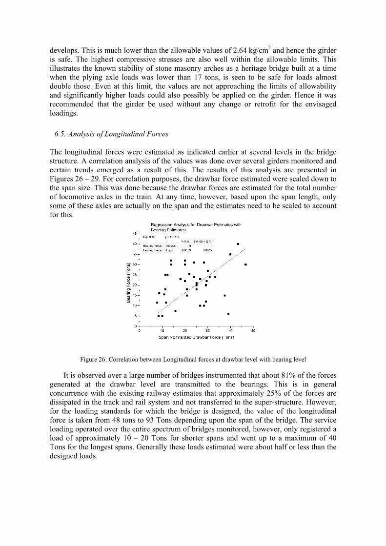
6.5. Analysis of Longitudinal Forces

The longitudinal forces were estimated as indicated earlier at several levels in the bridge structure. A correlation analysis of the values was done over several girders monitored and certain trends emerged as a result of this. The results of this analysis are presented in Figures 26 – 29. For correlation purposes, the drawbar force estimated were scaled down to the span size. This was done because the drawbar forces are estimated for the total number of locomotive axles in the train. At any time, however, based upon the span length, only some of these axles are actually on the span and the estimates need to be scaled to account for this.

Figure 26: Correlation between Longitudinal forces at drawbar level with bearing level

It is observed over a large number of bridges instrumented that about 81% of the forces generated at the drawbar level are transmitted to the bearings. This is in general concurrence with the existing railway estimates that approximately 25% of the forces are dissipated in the track and rail system and not transferred to the super-structure. However, for the loading standards for which the bridge is designed, the value of the longitudinal force is taken from 48 tons to 93 Tons depending upon the span of the bridge. The service loading operated over the entire spectrum of bridges monitored, however, only registered a load of approximately 10 – 20 Tons for shorter spans and went up to a maximum of 40 Tons for the longest spans. Generally these loads estimated were about half or less than the designed loads.

Figure 27: Correlation between Longitudinal forces at Super-Structure level with bearing level

From an analysis of the correlation of forces between the rocker bearings on an open-

web girder with the out-of-balance horizontal forces at the end portal at the rocker end as seen in Figure 27, it is seen that about 82% of the force coming on the bearing is transferred through the truss action of the open web girder. The remainder is possibly transferred through a complex series of actions including the shear forces in the members and the floor system.

Figure 28: Correlation between Longitudinal forces at Sub-Structure level with Rocker bearings

Figure 29: Correlation between Longitudinal forces at Sub-Structure level with Sliding bearings

The analysis of the forces transferred in the sub-structure as correlated with the

bearings are given in Figure 28 and Figure 29. From here it is seen that in a bridge having a rocker bearing, almost the entire force as is measured on the rocker bearing is transferred to the pier. This makes engineering sense as it is expected that most of the horizontal force would be transferred at the rocker with significantly lower interaction due to roller end fixities. As the pier has a rocker on one side and a corresponding roller on the other, it can be inferred that the coloring of the data due to the effect of the lower is fairly small (less than 10%). However, in the case of sliding bearings, the force is expected to be equally transferred at both ends and hence the correlation between the bearing force (assuming algebraic addition at both ends) and the pier shows that the pier actually attracts only about 50 – 60% of the total forces on the span. Piers are hence expected to be more critically loaded in spans having rocker bearings than in spans having sliding bearings.

This is an important conclusion, as it is seen that the horizontal load is only marginally due to the actual longitudinal loads applied. Significant amounts of horizontal loads are generated due to fixities in the bearings – as predicted from the converged numerical models, which although generally conservative for super-structure design, can be detrimental for the sub-structures.

6.6. Computation of Dynamic Augment

The Indian Railway bridge code prescribes that the railway bridges should be designed for dynamic effects which are due to the speed of movement of the train on the bridge. The codal provision for this is in the form of a quasi-static augmentation of the live load by a factor which is dependent upon the span of the girder and its corresponding length of influence line. The length of the influence line is termed as the loaded length and the augment factor is defined as:-

8 0.15

6CDA coefficient of dynamic augment

L

(1)

For a bridge of span 12.2 meters, this works out to an additional augment of 0.59 or an

additional 59% of live load. This reduces to a value of 30% for a 47.24 meter girder, but still is significantly high.

For each bridge under consideration, a train comprising the same set of loads was operated at speeds ranging from a crawling speed – simulating a quasi-static load condition – to the limit of the track design speed for the bridge under consideration. This varied from 65 kmph to 95 kmph for the bridges studied. Under all the conditions of operation, there was no significant increase in the measured stresses attributable to the speeds of operation in the super-structure. The results for the analysis are given in Tables 5 and 6. The results in these tables correspond to a design train of 2 locomotives leading followed by 55 wagons and 2 locomotives bringing up the rear adding up to a total of 244 axles on a 18.3 meters span plate girder.

Table 5: Analysis of Augment at Rail level

Maximum Minimum Mean Value Standard

Deviation

Codal Value for

Span and Speed

Slow Speed Run 16% -3% 6% 3% 7.67%

Design Speed Run 43% -3% 17% 5% 24.9%

Table 6: Analysis of Augment at Super-Structure locations

Crawling speed

Slow speed

Augment for slow speed

Fast speed

Augment for fast speed

Vertical Displacement at Center of Span (U/S)- -8.8 -9.0 2.3% -9.4 6.8%

Vertical Displacement at Center of Span (D/S) - -9.5 -9.5 0.0% -10.2 7.4%

Strain at Top Flange Center Span (U/S)- -115.0 -116.0 0.9% -123.0 7.0%

Strain at Bottom Flange Center Span (U/S)- 124.0 129.0 4.0% 133.0 7.3%

Strain at Top Flange Center Span (D/S)- -129.0 -131.0 1.6% -135.0 4.7%

Strain at Bottom Flange Center Span (D/S)- 123.0 128.0 4.1% 132.0 7.3%

Shear Strain at End Plate Pier (U/S)- -247.0 -246.0 -0.4% -247.0 0.0%

Shear Strain at End Plate Pier (D/S)- -255.0 -246.0 -3.5% -220.0 -13.7%

Shear Strain at End Plate Abutment (U/S)- 237.0 224.0 -5.5% 217.0 -8.4%

Shear Strain at End Plate Abutment (D/S)- 245.0 241.0 -1.6% 260.0 6.1%

As seen in Table 5, the maximum value of augment seen in the rail is as high as 43%,

although the mean values, though low, seem to generally agree with the codal requirements. These values are not isolated and similar trends are seen in other bridges instrumented. The

average values of augment measured for design speed runs are in the region of 15% - 30% for different bridges and the values of augment in the rail go up to as high as 70%. From Table 6, it is seen that the highest value of augment measured is just about 7.4%, while the average value of augment for slow speed is 0.2% while for fast speed the average value measured is 2.4%. In both cases, they are significantly lower than the codal predictions of 7.67 % and 24.9 % respectively.

It was thus inferred that the dynamic augment, although present in the rail, is dissipated due to the flexible connections between rail, sleepers, ballast, etc. and the super structure does not actually experience the supposed increase in responses due to these loads.

It was hence concluded, that although the track design speed has significant implications for the rail and track structure, the bridge super-structure and other componenets are relatively unaffected by this quantity. However, the flip side of this analysis was that since the girders were designed for this supposed augment values which actually didn’t transpire, they were sufficient for the periodic increases of loads imposed upon them. Many of the bridges were built as per a loading standard comprising an axle load of 17 Tons and the current axle loads plying these girders are 22.8 Tons – which is an increase of 34% – without any significant signs of distress.

7. Conclusions

The methods and techniques outlined above have been performed on a large number of bridges, as has been described in this paper. Consistent results have been obtained over the entire set of application making these robust techniques for evaluation of bridge structures. Significant and valuable information can be inferred from these applications, which can help enhance the infrastructure by estimating rational and appropriate mantainence strategies. It is also seen that naïve estimates need to be fine-tuned as they may be over conservative in some cases, while being inadequate in some others. The cost of this type of error can be very significant while dealing with sensitive infrastructure systems.

Some significant insights generated from the applications were:

1. It is possible to design structural health monitoring strategies that can deliver the outcomes that the client requires, while providing an effective bridge stock management tool.

2. The dynamic impacts which are still being used for load augmentation on bridges were found to be insignificant for the super-structure. They, however, were found to be present in the rail. So, although the super-structure is not adversely affected by the effects of design speeds within the current limits, the rail comes under significant stresses due to this aspect.

3. The longitudinal forces were seen to be significantly lower than the design values – to the tune of about 50%. However, there were seen to be significant values of horizontal forces generated due to fixities at the bearing level. These fixities, although reducing the stresses in the super-structure, increase the demand from the piers and abutments in some cases.

4. Some of the assumptions for design of railway girders are overly conservative – typically the longitudinal load and the dynamic augment values – however, the fixity effects may lead, in certain cases, to non-conservative estimation of service loads.

Acknowledgements

The authors gratefully acknowledge the permission given by Indian Railways to monitor the bridges presented in this study. The authors also acknowledge the efforts of everyone at InI Consulting, Mumbai, in assistance to monitor the bridge and collecting all the data used in this study. The help given and active participation by the Railway staff and all the employees of InI consulting has been invaluable in the successful completion of this study.

References

[1] Banerji, P., & Chikermane, S. (2009a). Structural Parameter Estimation of Two Bridges from Site Data using an Eigen Value Realization Algorithm, 4th International Conference on Structural Health Monitoring on Intelligent Infrastructure (SHMII-4), Zurich. [2] Banerji, P., & Chikermane, S. (2009b). Structural Parameter Estimation of Two Bridges from Site Data using Kalman Filters and Stochastic Subspace Algorithm, IV ECCOMAS Thematic Conference on smart structures and materials (smart’09), Porto [3] Banerji, P., & Chikermane, S. (2011). Structural Health Monitoring of a Steel Railway Bridge for Increased Axle Loads. Structural Engineering International 21(2), 210 – 216. [4] Banerji, P., & Chikermane, S. (2012). Condition assessment of a heritage arch bridge using a novel model updation technique. Journal of Civil Structural Health Monitoring 2(1), 1 – 16. [5] Chaminda, S. S., Ogha, M., Dissanayake, R., & Taniwaki, K. (2007). Different approaches for remaining fatigue life estimation of critical members in railway bridges. International Journal of Steel Structures KSSC 7 263 – 276. [6] Chan, T. H., Li, Z. X., & Ko, J. M. (2001). Analysis and Life Prediction of Bridges with Structural Health Monitoring Data- Part II: Application. International Journal of Fatigue 23(1) 55 – 64. [7] Li, Z. X., Chan, T. H., & Ko, J. M. (2001). ). Fatigue Analysis and Life Prediction of Bridges with Structural Health Monitoring Data- Part I: Methodology and strategy. International Journal of Fatigue 23(1) 45 – 53. [8] Miner. (1945). Cumulative Damage in Fatigue. Journal of Applied Mechanics, ASME, 12(3) A159 – A164. [9] Yanev, B. (1998). The Management of Bridges in New York City. Engineering Structures 20(11) 1020 – 1026.