Structural Estimation of a Flexible Translog Gravity Model
44
Structural Estimation of a Flexible Translog Gravity Model Shawn W. Tan * The World Bank December 2013 Abstract Arkolakis, Costinot and Rodriguez-Clare (2012) show that many quantitative trade models that summarize trade responses via a single elasticity have the same welfare implications. I develop a flexible approach to estimating trade responses using a translog expenditure function, and find welfare results that differ starkly from conventional trade models. In my model, trade responses can vary bilaterally, and the link between own- and cross-price elasticities of trade to trade cost is broken. I structurally estimate the parameters and conduct counterfactual analyses. Welfare responses are larger and more heterogeneous than those implied by the formula in Arkolakis et al. Keywords : Gravity model, Translog expenditure function, Structural estimation, Gains from trade. * Email: [email protected]. I am grateful to Russell Hillberry for his guidance and support. I also thank Andrew Clarke, Ed Balistreri, Chris Edmond, Simon Loertscher, Phillip McCalman, and seminar participants at the University of Melbourne microeconometrics seminar, the 2012 Australasian Trade Workshop, the 2012 Asia Pacific Trade Seminar, and the 2012 Econometric Society Australian Meeting for their helpful comments and suggestions. The findings, interpretations, and conclusions expressed in this article are entirely those of the author. They do not necessarily represent the views of the World Bank, its Executive Directors, or the countries they represent.
Transcript of Structural Estimation of a Flexible Translog Gravity Model

Structural Estimation of a Flexible Translog
Gravity Model
Shawn W. Tan∗
The World Bank
December 2013
Abstract
Arkolakis, Costinot and Rodriguez-Clare (2012) show that manyquantitative trade models that summarize trade responses via a singleelasticity have the same welfare implications. I develop a flexibleapproach to estimating trade responses using a translog expenditurefunction, and find welfare results that differ starkly from conventionaltrade models. In my model, trade responses can vary bilaterally, andthe link between own- and cross-price elasticities of trade to tradecost is broken. I structurally estimate the parameters and conductcounterfactual analyses. Welfare responses are larger and more heterogeneousthan those implied by the formula in Arkolakis et al.
Keywords: Gravity model, Translog expenditure function, Structuralestimation, Gains from trade.
∗Email: [email protected]. I am grateful to Russell Hillberry for his guidance andsupport. I also thank Andrew Clarke, Ed Balistreri, Chris Edmond, Simon Loertscher, PhillipMcCalman, and seminar participants at the University of Melbourne microeconometricsseminar, the 2012 Australasian Trade Workshop, the 2012 Asia Pacific Trade Seminar, andthe 2012 Econometric Society Australian Meeting for their helpful comments and suggestions.The findings, interpretations, and conclusions expressed in this article are entirely those ofthe author. They do not necessarily represent the views of the World Bank, its ExecutiveDirectors, or the countries they represent.

A central question in international economics is how best to measure the
gains from trade. A workhorse empirical tool to measure welfare gains in
international trade is the empirical gravity model of trade. A wide variety of
theoretical models provide microeconomic foundations for the gravity model
and interpret the bilateral trade pattern1. Despite many different motivations
for trade, recent work by Arkolakis, Costinot and Rodriguez-Clare (2012) has
shown that a broad class of quantitative trade models have equivalent macro-
level implications for the welfare gains from trade2. Among other common
features, all these models summarize trade responses via a single elasticity.
This elasticity also summarizes both the own- and cross-price responses of
trade to changes in trade costs3.
The use of a single parameter to summarize trade responses is an assumption
of convenience, not necessity. A single parameter simplifies theoretical derivations
and provides applied researchers with a parsimonious framework for estimating
trade responses. But trade responses to geographic frictions can vary across
importers and exporters, suggesting that a more flexible approach to estimation
may be preferable. I develop a flexible approach that allows trade responses
to vary bilaterally. This approach also breaks the link between own- and
cross-price elasticities of trade to trade costs. As a result, the welfare responses
differ from other quantitative trade models.
The flexible approach augments a standard gravity model with a more1Examples include Anderson (1979) and Krugman (1980) to more recent works by
Anderson and Van Wincoop (2003), Eaton and Kortum (2002), and Melitz (2003).2Arkolakis et al. (2012) restrict their analysis to trade models that satisfy three macro-level
restrictions: trade is balanced, profits are a constant share of GDP, and the import demandsystem is CES.
3The own-price elasticity of trade is the elasticity of imports with respect to variable tradecosts as it characterizes the response of import demand to its own price. The cross-priceelasticity of trade is the substitution elasticity between goods as it describes the response ofimport demand to the price of other goods.
1

flexible demand system, by representing the expenditure function with a
translog form. In general, the translog form does not impose any a priori
restrictions on elasticities. Novy (2013) derives and estimates a gravity model
that uses the translog form, but he does so in a context that leaves many
strengths of the translog form unexploited. In order to estimate the gravity
equation using ordinary least squares (OLS), Novy restricts the translog form
so as to generate a single structural parameter that can be recovered from the
data. While own- and cross-price effects differ in his framework, they do so by
a constant multiple — the substitution matrix contains a single value along
the diagonal and a single value off the diagonal. Arkolakis et al. (2010) show
that the translog form, with the parsimony achieved under the same estimating
restrictions Novy imposes and an assumption of a Pareto distribution of firm
productivity, implies the same welfare implications as other gravity models.
In contrast, my work follows the Diewert and Wales (1988) approach to
fitting a semi-flexible version of the translog form. This approach offers sufficient
flexibility to generate a rich substitution matrix. The restrictive substitution
pattern imposed elsewhere in the literature is a permitted special case but
importantly is not imposed at the outset. Indeed my empirical results suggest
that a richer substitution matrix than is assumed in the simpler models is an
important feature of the data. An added bonus of my approach is that both
the theory and the estimating model allow zero trade flows, and these zeroes
can be directly included in the estimation4.
The estimation technique involves the solution of a mathematical program
with equilibrium constraints (MPEC) as proposed by Judd and Su (2012).4Anderson and van Wincoop (2004), Haveman and Hummels (2004), and Helpman, Melitz
and Rubinstein (2008) have highlighted the prevalence of zeroes in bilateral trade flows andsuggested theoretical interpretations for them.
2

This structural estimation approach has the benefit of ensuring full theoretic
consistency5. Some papers have applied the MPEC approach to estimate
general equilibrium models of bilateral trade (Balistreri and Hillberry, 2007;
Balistreri, Hillberry and Rutherford, 2011), but those papers estimate trade
models with a single elasticity. I extend these methods to estimate a translog
gravity model.
I estimate the model on international flows between OECD and BRICS
countries from the UN COMTRADE. My empirical results suggest a rich
substitution pattern in the bilateral trade data. Given this rich substitution
pattern, the theoretical link between a given trade shock and welfare that is
the basis of Arkolakis et al. (2012) no longer holds. I conduct theory-consistent
counterfactual exercises and examine the welfare loss from more restricted
trade by (i) raising the import barriers of each OECD and BRICS country, and
(ii) increasing the trade barriers of China.
Not surprisingly, all countries lose from more restricted trade but the welfare
losses are larger and more heterogeneous than implied by the welfare result
in Arkolakis et al. (2012). Their formula, henceforth called the ACR formula,
establishes a linear relationship between a country’s expenditure on its home
goods and the own-price elasticity of imports. When elasticities are allowed
to vary in the translog model, this relationship no longer holds. The intuition
for the different results is that the translog form requires larger implied trade
costs to account for missing trade because trade responses of the large bilateral
flows are smaller than in the CES case.
Compared to the calculations using the ACR formula, the counterfactual5It also allows a straightforward and transparent link between the estimating model and
the counterfactual model. See Balistreri and Hillberry (2008) for a discussion of this issue inthe context of the Anderson and Van Wincoop (2003) gravity model.
3

welfare calculations have a higher average welfare losses and are more heterogeneous
than implied by the formula. When trade barriers are increased by 50 percent
for each country at a time, the average welfare loss across the countries is 26
percent according to the counterfactual calculations, and 2.6 percent according
to the formula calculations. The range of welfare losses is 4.7 to 32.9 percent
in the counterfactual calculations, and only 2.1 to 3.0 percent in the formula
calculations. When China retreats from the world market, the average welfare
loss for the rest of the world is 0.6 percent according to the counterfactual
calculations, and 0.06 percent according to the formula calculations. The range
of welfare losses is 0.02 to 1.52 percent in the counterfactual calculations, and
only 0.05 to 0.07 in the formula calculations.
The key distinction of the translog model is that trade responses are
not summarized by a single elasticity parameter: trade responses can vary
bilaterally. Despite different motivations for trade in many trade models, a
single structural parameter is often used to govern the responsiveness of trade
to changes in trade costs for a parsimonious framework in estimation6. But
it is unrealistic to assume that every country has the same trade responses,
regardless of country size and distance to market. Changes in trade costs will
affect relative prices, causing consumers to substitute between goods. A single
elasticity implies that changes to the demands for these goods will be the same.
The remainder of the paper is organized as follows. Section 2 provides a
motivation for relaxing the assumption of a single trade response in the gravity
model. The flexible approach is developed in Section 3, and compared to Novy6Anderson (1979) and Bergstrand (1985) assume an Armington product differentiation
based on country of origin to derive their gravity equations. Subsequent studies introducedmore complex production structures to the gravity model: monopolistic competition(Bergstrand, 1989); Heckscher-Ohlin (Deardorff, 1998); a multi-product and multi-countryRicardian model based on Dornbusch, Fischer and Samuelson (1977) (Eaton and Kortum,2002); and heterogeneous firms (Melitz, 2003 and Helpman, Melitz and Rubinstein, 2008).
4

Table 1: Estimates of Distance Elasticities
Dependent variable: ln xij (1) (2) (3) (4) (5)ln distij -0.531 -1.235 -0.681 -2.422 -2.715
(0.05) (0.03) (0.33) (0.32) (0.53)Constant 17.58 25.17 20.45 35.87 38.67
(0.39) (0.37) (2.95) (2.88) (4.74)Fixed Effects? No Yes Yes Yes YesImporter Interaction terms? No No Yes No YesExporter Interaction Terms? No No No Yes YesF-test∗ - - 0.00 0.00 0.00R2 0.069 0.901 0.916 0.920 0.934N 1482 1482 1482 1482 1482
Notes: Dependent variable is ln xij , the log of bilateral shipment between OECD and BRICScountries. Column (2) to (5) includes origin and destination fixed effects. Interaction termsare bilateral distance interacted with importer and exporter dummy variables. Standarderrors are in parentheses. All coefficients are significant at the five percent level. ∗P-value forjoint test of significance of distance interaction terms. Details on data is provided in theappendix.
(2013). Section 4 describes the structural estimation method and identification
strategy. Section 5 estimates the model and explores the effects of higher trade
restrictions with two counterfactual analyses. Section 6 concludes.
2 Motivation
In order to illustrate variability in trade responses, I regress the log of shipments
on bilateral distances in a fixed effects model. The specification is a simple
gravity equation where the trade costs is represented with just bilateral
distances. In order to capture the possibility of different elasticities for each
importer, I interact distance with importer dummy variables in the gravity
equation. The same data is used as in Section 5 and the data is described in
the appendix.
The regression results, presented in Table 1, show that each importer has a
5

different trade response. The inclusion of the distance and importer dummy
interaction terms in column (3) does not change the standard relationship that
exists between bilateral shipments, distances and home consumption. An F-test
on the joint significance of the interaction terms rejects the null hypothesis,
indicating that at least one importer has a different distance coefficient.
The distance coefficients do not, however, directly inform us whether there
are different own-price elasticities. From the theoretical models, the distance
coefficient is identified as a product of two parameters: the distance elasticity
of trade costs and the own-price elasticity of imports. But if we assume that
each importer has the same distance elasticity, we can attribute the different
distance coefficients to different own-price elasticities of imports.
Column (4) of Table 1 shows that elasticities can also differ for each exporter.
The F-test on the joint significance of the exporter interaction terms also fails
to reject the null hypothesis. Column (5) presents the results when the distance
terms are interacted with both exporter and importer dummy variables. These
interaction terms are jointly significant. That the elasticities can differ by
exporter should not surprise the reader since supply can also react differently
to changes in trade costs. While allowing for the elasticities to vary on the
demand and supply side will enrich the trade model, it can complicate the
analysis. We will focus on a model that allows the elasticities of importers to
vary and examine how the model differs from the standard trade model.
3 An Armington Trade Model with Translog Preferences
3.1 Theory
The theory is motivated via Armington preferences as in Anderson (1979): the
model assumes Armington preferences over the goods differentiated by origin
(Armington, 1969). Let there be n = 1, ..., N countries, and each country is
6

endowed with an amount of a good that is differentiated by country of origin.
Each country consumes N number of goods, including its own, but consumption
depends on prices, and prices depend on iceberg trade costs. The point of
the exercise is to minimally adjust the canonical Anderson and Van Wincoop
(2003) framework to illustrate the implications of flexible parameterization of
the representative consumers’ preferences7. The exercise also allows us to use
the Arkolakis et al. (2012) framework to understand welfare implications of
less restrictive assumptions about demand side behavior8.
The representative consumer’s utility maximization problem generates an
import demand and is expressed as its dual, the unit expenditure function. I
represent the unit expenditure function with a translog functional form, which is
a second-order approximation with respect to prices of an arbitrary expenditure
function (Diewert, 1976). Flexible functional forms, like the translog form,
do not impose any restrictions but are still consistent with the assumptions
inherent in the approximated functions.
The translog expenditure function is defined as:
lnEj = ξ +N∑n=1
αn ln pnj + 12
N∑n=1
N∑k=1
βnk ln pnj ln pkj (1)
7One could posit other theories of bilateral trade (Eaton and Kortum (2002); Melitz(2003) and Chaney (2008)) but my purpose is to work from the Anderson and Van Wincoopframework.
8Arkolakis et al. (2012) and Feenstra (2010) demonstrate that the single elasticityparameter models have similar welfare implications, regardless of whether the gains aredemand-side (consumer) or supply side (producer) gains. ? also show that there can bedifferent aggregate welfare results with different supply side assumptions, while still adoptinga CES demand side structure. I introduced flexibility on the demand side to illustrate thebenefits of parameter flexibility and examine the changes to welfare levels when trade costschange.
7

with these restrictions
N∑n=1
αn = 1,N∑k=1
βnk = 0, βnk = βkn ∀n, k = 1, ..., N (2)
imposed to fulfill homogeneity and symmetry conditions, where n, k indexes
the goods. The parameters in the translog function are analogous to those in
the CES unit expenditure function9. The αn parameters are the preference
weights for country n’s goods, and the βnk parameters inform us about the
substitutability between goods n and k.
The destination price pnj = pnτnj is the trade-cost inclusive price of good
n in country j, where pn is the free-on-board (f.o.b.) price of good n, and
τnj is the costs of trading the goods between countries n and j. Trade cost is
assumed to be an iceberg cost where τnj is the amount of good required to ship
one unit of the good from n to j, i.e. τnj > 1, ∀n 6= j, otherwise τjj = 1.
Expenditure functions are concave in prices and this property is achieved in
the translog expenditure function if the Hessian matrix is negative semidefinite,
i.e. the second order partial derivatives with respect to prices ∇pnjpkjEj are
negative semidefinite. The concavity property is maintained in the translog
expenditure function by imposing the restrictions from Diewert and Wales
(1988) in the estimation, which will be discussed in Section 410.
Applying Shephard’s Lemma to equation (1), the import share equation
9The CES expenditure function is defined as Ej =[∑N
n (θpnj)1−σ] 1
1−σ .10It is a common issue that the curvature conditions of theoretical functions are not satisfied
by the unrestricted translog function. I use the restrictions in Diewert and Wales (1988)because it maintains the flexibility of translog function, while achieving global concavityin prices. There are two alternative methods to impose concavity on the translog form.Restrictions can be placed on the translog function to impose global concavity but this mightremove the flexibility of the form (Diewert and Wales, 1987). Conversely, restrictions can beplaced at a single observation, which maintains the flexibility of the translog function butonly imposes concavity locally (Ryan and Wales, 2000).
8
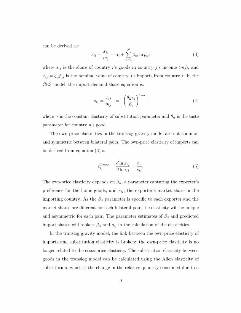
can be derived as:
sij = xijmj
= αi +N∑n=1
βin ln pnj (3)
where sij is the share of country i’s goods in country j’s income (mj), and
xij = qij pij is the nominal value of country j’s imports from country i. In the
CES model, the import demand share equation is:
sij = xijmj
=(θipijEj
)1−σ
, (4)
where σ is the constant elasticity of substitution parameter and θn is the taste
parameter for country n’s good.
The own-price elasticities in the translog gravity model are not common
and symmetric between bilateral pairs. The own-price elasticity of imports can
be derived from equation (3) as:
εTransij = d ln xijd ln τij
= βiisij. (5)
The own-price elasticity depends on βii, a parameter capturing the exporter’s
preference for the home goods, and sij, the exporter’s market share in the
importing country. As the βii parameter is specific to each exporter and the
market shares are different for each bilateral pair, the elasticity will be unique
and asymmetric for each pair. The parameter estimates of βii and predicted
import shares will replace βii and sij in the calculation of the elasticities.
In the translog gravity model, the link between the own-price elasticity of
imports and substitution elasticity is broken: the own-price elasticity is no
longer related to the cross-price elasticity. The substitution elasticity between
goods in the translog model can be calculated using the Allen elasticity of
substitution, which is the change in the relative quantity consumed due to a
9

one percent change in the relative prices. From Berndt (1991), The formula
for the Allen elasticity between goods i and j:
σij = βij + sijsjjsijsjj
∀i, j and i 6= j, (6)
while the own elasticity of substitution (i.e. with its own prices) equals:
σii = βii + s2ii − siis2ii
. (7)
A positive elasticity indicates that the goods are substitutes where an increase
in the price of good i will increase the demand for good j. Given empirical
estimates of βij and fitted sij, the elasticities can be easily calculated.
The elasticities in the translog model are different from those in Novy (2013).
While Novy has a model with differentiated product varieties, he uses a measure
of extensive margin to simplify the estimation. The own-price elasticity of
imports in his model is:
εNovyij = d ln sijd ln τij
= −γgisij
, (8)
where gi is a measure of the extensive margins of the exporting country, and
γ is a parameter from the restrictions Novy places on the translog function.
The measures of extensive margins are taken from data so Novy essentially
estimates a single parameter in his gravity estimation 11.11It may not be suitable to use this measure of extensive margins given that it implicitly
assumes each country is exporting the entire product range to every country. Whereasthe numerator in equation (5) is an estimated parameter that varies with exporters, thenumerator in Novy’s own-price elasticity varies only by the extensive margin. Moreover,Novy develops his model assuming monopolistic competition. In a model with Armingtongoods, the extensive margin measure will be absent in equation (8) and variation in theelasticities will depend solely on the import share values.
10

The own-price elasticity of imports derived in this paper gives a nuanced
description of trade responses. It captures the tension between how much
of a good is consumed at home and how much of it is consumed in foreign
markets. The βii parameter summarizes an exporter’s preference for its home
good, which determines how much it exports. The market share (sij) describes
the consumption share of the good in the importing country. The own-price
elasticity of imports also captures the effects of distance and country size on
trade flows through the market share parameter. If the exporter is near the
destination market, the short distance will lessen trade costs and keep the
destination prices low. Similarly, if the exporter is a large country, it can sell
the good at a low f.o.b. price because a substantial home market can produce
economies of scale. Although scale economies are absent in the model, they are
present in the data and the model may pick up this feature in the estimation.
Lastly, if the importing country is small, an exporter is more likely to capture
a sizable market share. In these three cases, the exporter’s market shares will
be large, indicating that these trade flows will be relatively inelastic.
For example, Australia is a large and relatively open country that exports
about 75 percent of its production of goods. It can command a large market
share in the New Zealand market because it is close-by and a small market.
New Zealand is also remote and lacks access to other low costs suppliers.
Therefore, New Zealand’s demand for Australian imports will be relatively
inelastic. Conversely, Australia will only capture a small percent of the U.S.
market because of the distance and sheer size of that market. The U.S. demand
for Australian imports will then be relatively elastic12. In the CES model, by12The Armington assumption classifies the bundle of goods from a country as the national
good so another way to interpret the inelastic U.S. demand for Australian imports is thatwithin the American bundle of goods, there is one good that is highly substitutable with theAustralian good.
11

contrast, the demand for Australian imports by New Zealand and the U.S. will
be the same: the import demands of these two countries will react in the same
fashion to an increase in trade costs and imports from Australia will decrease
by the same proportion.
The own-price elasticity of imports also captures aspects of market competition.
An exporter that is a large seller in a market will face less competition and
have a more inelastic demand in that market. Conversely, for an exporter that
is a small seller, the competition is higher and there is a more elastic demand
for its goods. Relative to an exporter with a small market share, an increase
in trade costs will have a smaller impact on an exporter with the larger market
presence because it can pass on the higher trade costs to the consumers13.
3.2 Model’s Implications
In many empirical gravity models of trade, Arkolakis et al. (2012) show that
changes in welfare levels can be captured with just two statistics: the change
in the expenditure on home goods and the own-price elasticity of imports. The
ACR formula summarizes the welfare effects of a change in trade costs:
Wj = 1−(λjjλ
′jj
)1/ε
, (9)
where λjj and λ′jj are a country’s expenditure on home goods before and after
changes in trade costs, and ε is the elasticity of imports with respect to trade
costs (or own-price elasticity of imports). In the CES model, εCES = 1− σ so
there is a linear relationship between the welfare effects of a change in trade13Edmond, Midrigan and Xu (2012) examine this insight with a richer model that includes
firm activities. They derive an elasticity of imports with respect to trade costs that dependson the import shares in an industry and the reallocation of expenditure between industries.They use firm level data to estimate the varying elasticities, while I will be estimating theelasticities from aggregate trade data.
12

costs and changes in openness(λjj
λ′jj
).
In fact, the result in Arkolakis et al. (2012) is more general: one does
not need to know the origin of the shock, whether it is a change in the trade
costs with one trade partner or a proportional change across all partners, the
formula summarizes the welfare effects of that shock14. These two variables
are sufficient for welfare analysis in these models because openness reflects the
change in traded goods and the elasticity is the change in the quantities due to
changes in prices (Imbs and Mèjean, 2011).
For the ACR formula to hold, the trade model must have an important
macro-level restriction — it must produce a CES import demand system. Such
an import demand system means that the bilateral imports are only affected
by changes to trade costs on that bilateral link, i.e. d lnxij
d ln τij= 1−σ. This import
demand system implies that the elasticity of bilateral imports with respect to
trade costs on another bilateral link (for example, countries k and j) is zero,
i.e. d lnxij
d ln τkj= 0 where i 6= k.
The welfare formula in Arkolakis et al. (2012) does not apply in my translog
gravity model. In this model, trade between countries i and j is affected by
trade costs between countries k and j. The model is more flexible than the CES
import demand system, which can be easily shown by taking the derivative of
the import demand:
εTransik = d ln xijd ln τkj
= βiksij≥ 0. (10)
As trade costs increase along the k-j link, country j can substitute away from
the goods of country k and increase its imports from country i.14The effects of a change in trade costs with one partner versus a proportional change
across all partners are different. With a change in trade costs with one partner, there will bea trade diversion effect, while there will not be one with the proportional change in tradecosts. The formula applies in both cases because it captures the diversion of trade towardsthe country’s home good.
13

The flexible import demand system is key to why this translog gravity model
has a different welfare implication from Arkolakis et al. (2012). Other gravity
models have incorporated a translog demand system but they still generate
the Arkolakis et al. (2012) welfare result because these models produce a CES
import demand system. Arkolakis et al. (2010) show that the ACR formula
can summarize welfare changes in a model with translog form and firm-level
varieties. They can obtain this result because they apply restrictions in Feenstra
(2003) on the translog form, which impose additional structure creating a CES-
like preferences15. Novy (2013) also has a translog gravity model with the
Feenstra (2003) restrictions. Even though Novy does not examine if the ACR
formula applies to his model, a simple check of the gravity equation shows
that his restricted translog model conforms to a CES import demand system16.
Thus, the Arkolakis et al. (2012) welfare result applies in Novy (2013): the
model has the same welfare implications as other quantitative trade models.
Without a CES import demand system, there is no equivalent statistic or
formula, like the ACR formula, that can summarize changes in welfare levels
in the translog model. Welfare calculations have to done using counterfactual
analyses. We can, however, expect that the welfare changes due to changes in
trade costs in the translog model to be heterogeneous compared to the CES
model. Heterogeneity in the changes of welfare levels is evident: importers in
the translog model have varying own-price elasticities so the changes in welfare
levels will not exhibit a clear linear relationship with a country’s consumption15The restrictions are on the substitution matrix of the expenditure function: a matrix
of the cross partial derivatives of the expenditure function with respect to the prices oftwo goods. The matrix is composed of all βnk parameters. The restrictions in Feenstra(2003) impose one value for the off-diagonal and one value for the diagonal elements. Thesubstitution matrix for a CES expenditure function will have σ on the off-diagonal andzeroes on the diagonal.
16See equation 7 in Novy (2013).
14

of its home goods.
We can also expect that the welfare changes to be larger in the translog
model. The magnitude of the welfare level changes depends largely on how the
changes in the trade costs affect the expenditure function. The CES expenditure
function only captures the direct effect of a change in trade costs on the price
of the affected goods. In contrast, the translog expenditure function contains
additional variables — the third variable on the RHS of equation (1) — that
capture the indirect, or substitution, effects of a change in trade costs. As
βnk ≥ 0 (∀n 6= k), any change in trade costs will be amplified in the translog
expenditure function since the direct and substitution effects move in the same
direction. With the same income levels, an increase in trade costs causes a
larger increase in the translog expenditure function, which results in larger
welfare losses compared to the CES model.
4 Estimating Framework
4.1 Structural Estimation
The estimation method depends on how the structure is imposed in the model.
Anderson and Van Wincoop (2003) show that the general equilibrium structure,
specifically the market clearance conditions, is important in the trade model,
and excluding the structure can create omitted variable bias in the estimation.
On the other hand, applying the market clearance conditions to the model
complicates the estimation because the new terms in the import demand
introduces non-linearity in the model17.
Several methods are used to deal with this issue, with fixed effects and non-17When the market clearance conditions are applied, multilateral resistance terms are
included into the import demand equation (Anderson and Van Wincoop, 2003). Thesemultilateral resistance terms capture the effects of relative prices in the model but alsointroduces non-linearity in the estimation as the terms are a function of each other and tradecosts.
15

linear estimation being the two most common18. With fixed effects methods,
the non-linear terms are captured with fixed effects. With non-linear estimation
methods, the non-linear terms, together with the gravity equation, are estimated
jointly as a system of equations.
Alternatively, the market clearance conditions can be applied directly as
constraints in the estimation. Balistreri and Hillberry (2007) develop a method
to do this and estimate a CES gravity model with Armington assumptions.
This method is essentially the MPEC approach discussed in Judd and Su
(2012). The MPEC approach guarantees full theoretic consistency of the fitted
values and the estimated parameters19. Although the empirical procedure is
conceptually similar to the non-linear least squares approach of Anderson and
Van Wincoop (2003), it presents an advantage when conducting counterfactual
analyses. The constraints define an operational general equilibrium that allows
for a simple transition from the estimation to the counterfactual analyses, which
is discussed later. It has also been used to estimate a model with monopolistic
competition and heterogeneous firms (Balistreri et al., 2011).
The estimating strategy in Balistreri and Hillberry (2007) is to minimize
the squared differences between the observed (zij) and fitted (zij) trade values:
min∑i
∑j
[zij − zij]2 , (11)
subject to the constraints implied in the model20. These constraints include a18There is a empirical method developed by Baier and Bergstrand (2009) that uses a
first-order Taylor-series expansion of the multilateral resistance terms to estimate the systemof gravity equations.
19The MPEC is used to solve a Walrasian general equilibrium here and in Balistreri andHillberry (2007), whereas the focus of MPEC estimation following Judd and Su (2012), hasbeen on partial equilibria, and more typically Nash equilibria.
20The structural estimation approach is set out in the appendix of Balistreri and Hillberry(2007).
16

market clearance condition where a country’s income is spent on all imports;
an income equation that relates real and nominal income; a unit expenditure
function that measures the cost of living; and a utility equation that describes
utility levels. While the market clearance conditions impose model structure
on estimation, the income equation, unit expenditure function, and utility
equation insure full theoretical consistency of the fitted general equilibrium.
Full consistency in estimation is important for subsequent counterfactual
analysis (Balistreri and Hillberry, 2008).
I adapt this estimation framework to the translog model. First, the fitted
values of the import share are defined according to the derived import share
demand in equation (3). Second, the translog unit expenditure function in
equation (1) is used. Third, the market clearance condition is modified to use
the fitted import share values. The constraints are:
yi = pimi ∀i, (12)
mi =∑j
sijmj ∀i, (13)
lnEj = ξ +N∑n=1
αn ln pnj + 12
N∑n=1
N∑k=1
βnk ln pnj ln pkj ∀j, (14)
UiEi = yi ∀i. (15)
Equation (12) defines the income of a country where yi and mi are the nominal
and real income of the country i. Equation (13) defines clearance in the goods
market. Equation (14) is the unit expenditure function, and equation (15)
defines the utility of country i where Ui is the utility level.
In addition, certain assumptions and normalizations in the model are made
to estimate the parameters. Following Balistreri and Hillberry (2007), the
GE model is normalized such that the choice of endowment units equal the
17

observed nominal income:
yi = mi ∀i, (16)
pi = 1 ∀i. (17)
The constant term in the unit expenditure function (ξ) is assumed to equal
one21. The homogeneity and symmetry restrictions from equation (2) are also
imposed in the estimation. To ensure that monotonicity conditions are met,
further restrictions are placed on the predicted import shares such that it is
between zero and one, and the shares in each importing country sums to one:
0 ≤ sij ≤ 1 ∀i, j (18)N∑j
sij = 1. (19)
As the import shares sum to one, an import share equation is dropped, otherwise
the variance-covariance matrix is singular. Choice variables in the estimation
are the coefficients in the import share equation (αn and βnk) and the general
equilibrium variables (Ui, pi, Ei and yi). The non-linear estimation is solved in
the GAMS software using the CONOPT algorithm.
For purposes of comparison, I also estimate a CES gravity equation with
the same method. The logarithm of the import shares are used, and the fitted
value in the minimization problem (11) is defined by taking the log of import21The ξ parameter is a common scalar across all countries and will shift the expenditure
functions in the same way. Assuming that ξ = 1 reduces the number of parameters to beestimated in the system and does not have any implications on the results. This is alsoconsistent with how a CES unit expenditure function will be expressed. Drawing an analogywith the CES unit expenditure function, the αn parameters are analogous to the weights inthe CES function; the βnk substitution parameters to the elasticity of substitution; and thatmeans that ξ in equation (1) is the scalar in the CES function, which equals one.
18

demand in equation (4):
ln sij = lnmj + (1− σ) [ln θi + ln pi + ln τij − lnPj] . (20)
Changes are made to the expenditure function and market clearance conditions
to reflect those in the CES model22. The importer income coefficient is also
restricted to one to be consistent with theory. The CES specification estimates
the values of σ and θi, conditional on the trade cost specification.
A key difference between the translog and CES formulations, and the
advantage of using the translog model, is the possibility of having zeroes in
the dependent variable. With the CES specification, the dependent variable
(sij) is in logarithm form and zeroes complicate the estimation and inference.
There are many strategies used in the literature to deal with zeroes: exclude
them from the estimation or add a small value to the zeroes. Alternatively, one
could use the pseudo-Poisson maximum likelihood approach set out by Santos
Silva and Tenreyro (2006) but they do not provide a theoretical reason for the
existence of zeroes in the data. With the translog model, zero trade flows are
possible in the theory because countries do not consume that particular good
and we can include the zeroes in the estimation23.
Trade costs are assumed to be a multiplicative function of distance and
home consumption: τij = distρij exp (δ)1−homeij where distij is the distance
between country i and country j; ρ is the distance elasticity of trade cost;
homeij is a dummy variable capturing home consumption where homeij = 1 if
the country is consuming home goods; and exp (δ) is the ad valorem tax for
22The CES expenditure function is defined as Ej =[∑N
n (θpnj)1−σ] 1
1−σ and the marketclearance conditions are mi =
∑j xij ∀i.
23It is also possible to assume a Poisson distribution for the error term in the estimationbut it is not done here.
19

crossing national borders.
Structural estimation of this sort facilitates counterfactual analysis in a
straightforward manner. The model used in counterfactual analysis is that
which appears in the constraints. Equations (12) to (15) impose constraints on
the estimation method to create an operational GE model. In the estimation
stage, income and prices are fixed and variables in the model are estimated. In
the counterfactual stage, the structural parameters are locked in while income
and prices are freed up for the counterfactual analysis. Changes are made
to trade costs in the general equilibrium model to reflect the counterfactual
scenarios, and the new equilibrium is solved. The percentage changes to income,
prices and utility are calculated by comparing the changes from the baseline
trade equilibrium to the counterfactual equilibrium levels.
Standard errors are calculated using bootstrapping techniques for all the
variables in the estimation. The uncertainty in our variable estimates is also
carried into the counterfactual calculations so bootstrapped standard errors
are also calculated for the counterfactual analyses24. For each iteration, a new
bootstrap sample is drawn with replacement from the original sample. The
process is repeated 1,000 times.
4.2 Identification Strategy
Estimation of gravity models in international trade is usually concerned with
identifying a single parameter — the elasticity of imports with respect to trade
costs. The single parameter models sometimes require additional assumptions
to be made in the theoretical model.
While the translog form allows us to move away from estimating a single
elasticity parameter, there is a challenge of separately identifying the variables24In the trade literature, standard errors are usually not calculated for the counterfactual
analyses but it should be.
20

in the trade cost specification and the import demand equation. This challenge
is common in the estimation of CES models and is not unique to the translog
model. When the trade cost specification is substituted into the import demand
equation, the unknown variables in trade costs (ρ and δ) interact with those in
the import demand equation: (1− σ) in the CES specification and βnk in the
translog specification.
Since there is not enough information in the data to separately identify the
parameters, a value for one parameter can be chosen to help with identification25.
Anderson and Van Wincoop (2003) assume a value for σ in their post-estimation
calculations. Balistreri and Hillberry (2007) impose the value σ = 5 pre-
estimation, but this is without consequence to the estimation. Since the
translog model does not contain the σ parameter, it is more sensible to impose
a ρ value in our estimation. I impose ρ = 0.267 in estimation, which is a
direct estimate of the distance elasticity of trade cost from freight costs data
(Hummels, 2001). The value is also used in Novy (2013).
In the translog expenditure function, the own-price elasticity of imports is
no longer restricted to be a single structural parameter. This flexibility, however,
complicates the estimation process. Estimating the full translog specification
with the parameter restrictions to ensure homogeneity and symmetry is
equivalent to estimating N(N+1)2 + N + 1 parameters: one δ parameter, N
an parameters, and N(N+1)2 βnk parameters, where N is the total number of
national goods in the model26. The degrees of freedom and the efficiency of
parameter estimates are greatly reduced compared to the CES specification.
Novy (2013) applies the restrictions in Feenstra (2003) to reduce the25By imposing a structural parameter in the estimation, we are mixing calibration and
estimation methods.26If there are 50 goods in the sample, the 2500 observations are used to estimate 1326
parameters.
21

parameters in the substitution matrix, an N ×N matrix of the βnk parameters.
The restrictions in Feenstra (2003) severely restrict the βnk parameters in the
substitution matrix to depend on a single parameter (γ) and the total number
of goods (G):
βNovynk = γ
G, ∀n 6= k (21)
βNovynn = − γG
(G− 1) . (22)
Thus, the substitution matrix will only possess two values: one along the
diagonal using equation (22) and one off the diagonal using equation (21).
These restrictions place an a priori assumption on the substitutability of the
goods: the same off-diagonal elements presupposes that each good is the same
substitute to every other good. This assumption is similar to a CES assumption.
It would be better to allow the data to inform us about the substitutability of
the goods. By using the extensive margin (G) in the restrictions, Novy also
implicitly assumes that each country exports the same number of goods to
every trade partner.
These restrictions help achieve parsimony in the model, but it is overly
restrictive and essentially returns us to a single parameter model. In his model,
Novy is estimating the value of γ. Although Novy starts with a model of
monopolistic competition, the restrictions simplify the model in such a way
that aggregate trade flows can be used27.
An alternative set of restrictions developed by Diewert and Wales (1988) is a
better approach to reduce the number of parameters in the substitution matrix.
These restrictions create a semi-flexible functional form, which is suited to deal
with large numbers of goods in translog specification. The form maintains some27A fixed effects model is estimated with aggregate trade flows between 28 OECD countries.
22

degree of flexibility while still being consistent with the concavity assumptions
required for the expenditure function.
Diewert andWales (1988) decompose the substitution matrix, B ≡ [βnk]N×N ,
into the product of a lower triangular matrix and its transpose:
B = −DDT (23)
where D is a lower triangular matrix of rank r ≤ N − 1 chosen by the
econometrician. They prove that the D matrix exists, and the semi-flexible
functional form can approximate a differentiable function up to the second
order. Relative to the fully flexible translog form, the number of parameters
to be estimated is greatly reduced. For example, choosing a rank one lower
triangular matrix reduces D to an N × 1 vector, and if N = 50, only 101
parameters need to be estimated instead of 1326 parameters in the fully flexible
translog form. The restrictions also constrain the substitution matrix to be a
negative semidefinite matrix, which ensures that the expenditure function is
concave in prices.
The semi-flexible functional form has been successfully used to estimate
translog demand systems with many goods. Kohli (1994) demonstrates that
the cost of using the semi-flexible functional form is small while the benefits
of increased efficiency are large. He does not find large differences in the
elasticities calculated with a low rank matrix compared to a higher rank matrix.
Neary (2004) uses this approach to estimate a Quadratic Almost Ideal Demand
and an Almost Ideal Demand systems. He begins his estimation with a rank
one matrix and uses the results as the starting value for the rank two matrix.
Neary continues this process to estimate the full rank substitution matrix.
While that is an innovative way to apply the Diewert and Wales approach,
23

Neary (2004) estimated the elasticities for eleven goods. His approach will be
difficult to implement given the large number of goods considered in this paper.
Instead, I use a rank one decomposition developed by Kee et al. (2008).
They apply the Diewert and Wales approach to estimate the import demand
equations for 4,900 goods. They reparameterize the substitution matrix by
imposing these constraints:
βnk = γbnbk, ∀n 6= k (24)
βnn = −γbn∑n6=k
bk, (25)
where γ, bn, and bk are constants. The reparameterization reduces the translog
function to be flexible of degree one. The constraints also satisfy the symmetry
constraints: βnk = βkn, and the homogeneity constraints: ∑k 6=n βnk + βnn = 0.
5 Rising International Trade Restrictiveness
5.1 Estimation Results
The estimation model covers 39 countries consisting of 34 OECD countries
and five BRICS countries in 200628. The BRICS countries are included in the
sample to make it a more representative data set. This sample expands the
subset of OECD countries examined in Eaton and Kortum (2002) and Novy
(2013). The 39 countries make up about 90 percent of the world’s GDP in
2006. The data sources are discussed in the appendix.
Before discussing the results, there is a matter in the construction of the28The 34 OECD countries are Australia, Austria, Belgium, Canada, Chile, Czech Republic,
Denmark, Estonia, Finland, France, Germany, Greece, Hungary, Iceland, Ireland, Israel,Italy, Japan, South Korea, Luxembourg, Mexico, Netherlands, New Zealand, Norway, Poland,Portugal, Slovak Republic, Slovenia, Spain, Switzerland, Turkey, United Kingdom, andUnited States. The five BRICS countries are Brazil, Russian Federation, India, China, andSouth Africa. The countries and their alpha-3 codes are listed in Table 2.
24

import share variables, which is the ratio of imports from country i (xij) and
expenditure of country j (mj). A country’s expenditure, measured as the value
of total imports, usually equals its income. There is, however, a discrepancy
between the expenditure and income of a country because, for example, of the
presence of non-traded service sectors or, in this case, an incomplete set of
import partners. The discrepancy between expenditure and income figures is
an issue in any estimation of the gravity model, but it becomes more important
here29. In the translog estimation, the import shares equal one and that allows
us to drop a share equation but that is not possible if income is larger than
expenditure. The solution taken in this paper is to create an artificial measure
of expenditure by aggregating a country’s import values (including its own
trade flows) and treating that as the country’s expenditure.
The translog estimates of αn and βnn are presented in Table 2. The αnparameters, which are common for all countries, inform us about the importance
of a country’s goods in the expenditure function. It is no surprise that the large
manufacturing countries have the largest weight: the U.S. (14 percent), Japan
(9 percent), China (8 percent), India (5 percent), and Germany (5 percent). βnnis presented for each importer and these are used to construct the elasticities.
Estimates for the own-price elasticities and the border taxes are presented
in Table 3. Conditional on the value of the distance elasticity of trade cost
(ρ = 0.267), the own-price elasticity from the CES model and the average
own-price elasticity from the translog model are similar in magnitude. The
CES estimate for the own-price elasticity is (1− σ) = −4.44 while the average
own-price elasticity from the translog model is −4.68. The CES elasticity of29Anderson and Van Wincoop (2003) face this issue in their estimation, but they did
not impose an aggregation constraint. The MPEC method requires consistency with allthe conditions of the model, including aggregation conditions, so I need to take a stand ondomestic trade flows.
25

Table2:
Parameter
Estim
ates
Cou
ntry
Cod
eα
nβ
nn
Cou
ntry
Cod
eα
nβ
nn
Cou
ntry
Cod
eα
nβ
nn
Australia
AUS
0.037
-0.05
5Greece
GRC
0.009
-0.02
7Norway
NOR
0.008
-0.03
1
(0.00
3)(0.00
7)(0.00
1)(0.00
5)(0.00
1)(0.00
6)
Austria
AUT
0.011
-0.03
7Hun
gary
HUN
0.006
-0.01
9Polan
dPOL
0.012
-0.04
2
(0.00
1)(0.00
5)(0.00
1)(0.00
3)(0.00
1)(0.00
6)
Belgium
BEL
0.017
-0.06
1Icelan
dISL
0.001
-0.00
5Portugal
PRT
0.009
-0.03
0
(0.00
2)(0.00
9)(0.00
0)(0.00
1)(0.00
1)(0.00
6)
Brazil
BRA
0.046
-0.08
6India
IND
0.052
-0.11
7Russia
RUS
0.028
-0.08
5
(0.00
4)(0.01
3)(0.00
2)(0.01
2)(0.00
2)(0.01
8)
Can
ada
CAN
0.044
-0.01
0Irelan
dIR
L0.0
06-0.02
6Slovak
Rep
SVK
0.003
-0.01
1
(0.00
2)(0.01
7)(0.00
1)(0.00
5)(0.00
0)(0.00
2)
Chile
CHL
0.009
-0.01
5Israel
ISR
0.006
-0.01
6Slovenia
SVN
0.002
-0.00
6
(0.00
1)(0.00
3)(0.00
1)(0.00
3)(0.00
0)(0.00
1)
China
CHN
0.079
-0.13
2Italy
ITA
0.039
-0.12
3So
uthAfrica
ZAF
0.019
-0.03
6
(0.00
3)(0.02
2)(0.00
1)(0.02
1)(0.00
3)(0.00
8)
Czech
Rep
CZE
0.007
-0.02
3Ja
pan
JPN
0.089
-0.16
3Sp
ain
ESP
0.036
-0.12
4
(0.00
1)(0.00
3)(0.00
5)(0.02
2)(0.00
1)(0.02
4)
Denmark
DNK
0.008
-0.02
8Korea
KOR
0.035
-0.06
9Sw
eden
SWE
0.013
-0.04
7
(0.00
1)(0.00
4)(0.00
1)(0.00
8)(0.00
1)(0.00
8)
Eston
iaEST
0.001
-0.00
4Lu
xembo
urg
LUX
0.001
-0.00
4Sw
itzerlan
dCHE
0.009
-0.03
3
(0.00
0)(0.00
1)(0.00
0)(0.00
1)(0.00
1)(0.00
6)
Finland
FIN
0.009
-0.03
1Mexico
MEX
0.041
-0.07
7Tu
rkey
TUR
0.021
-0.06
1
(0.00
1)(0.00
6)(0.00
2)(0.01
1)(0.00
2)(0.01
0)
Fran
ceFRA
0.038
-0.13
1Netherlan
dsNLD
0.018
-0.06
7UnitedKingd
omGBR
0.039
-0.14
7
(0.00
1)(0.02
3)(0.00
2)(0.00
9)(0.00
2)(0.03
1)
German
yDEU
0.049
-0.16
6New
Zealan
dNZL
0.007
-0.00
9UnitedStates
USA
0.141
-0.25
4
(0.00
3)(0.03
4)(0.00
1)(0.00
1)(0.01
8)(0.05
5)
Notes:Boo
tstrap
pedstan
dard
errors
arein
parentheses.
Allcoeffi
cients
aresign
ificant
atthefiv
epe
rcentlevel.
Cod
esarealph
a-3
coun
trycodes.
26
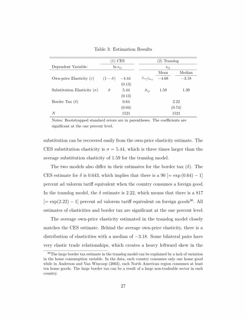
Table 3: Estimation Results
(1) CES (2) TranslogDependent Variable: ln sij sij
Mean MedianOwn-price Elasticity (ε) (1− σ) −4.44 βnn/snj −4.68 −3.18
(0.13)Substitution Elasticity (σ) σ 5.44 σij 1.59 1.39
(0.13)Border Tax (δ) 0.64 2.22
(0.04) (0.74)N 1521 1521
Notes: Bootstrapped standard errors are in parentheses. The coefficients aresignificant at the one percent level.
substitution can be recovered easily from the own-price elasticity estimate. The
CES substitution elasticity is σ = 5.44, which is three times larger than the
average substitution elasticity of 1.59 for the translog model.
The two models also differ in their estimates for the border tax (δ). The
CES estimate for δ is 0.643, which implies that there is a 90 [= exp (0.64)− 1]
percent ad valorem tariff equivalent when the country consumes a foreign good.
In the translog model, the δ estimate is 2.22, which means that there is a 817
[= exp(2.22)− 1] percent ad valorem tariff equivalent on foreign goods30. All
estimates of elasticities and border tax are significant at the one percent level.
The average own-price elasticity estimated in the translog model closely
matches the CES estimate. Behind the average own-price elasticity, there is a
distribution of elasticities with a median of −3.18. Some bilateral pairs have
very elastic trade relationships, which creates a heavy leftward skew in the30The large border tax estimate in the translog model can be explained by a lack of variation
in the home consumption variable. In the data, each country consumes only one home goodwhile in Anderson and Van Wincoop (2003), each North American region consumes at leastten home goods. The large border tax can be a result of a large non-tradeable sector in eachcountry.
27

distribution31. There are fifteen pairs (or the top one percent) with elasticities
smaller than -28, with the most elastic pair being the Spain-U.S. with an
elasticity of -167. These pairs have exporters trading with large countries (the
U.S., Japan, and United Kingdom), resulting in small market shares and elastic
import demands.
Substitution elasticities are calculated for all country pairs with positive
predicted import shares using βij and sij . The average and median substitution
elasticities are 1.59 and 1.39 respectively. Positive elasticities indicate that
both goods in each bilateral pair are substitutes, a result that is consistent with
the Armington assumption. Most of the country pairs have elasticities below
10, with over 90 percent having elasticities below 2, and only four country
pairs have an elasticity above 1032. This implies that most pairs, despite being
substitutes as assumed in the Armington model, are not strong substitutes.
It is informative to examine the bilateral elasticities of a large country, say
China, to better understand its relationship with its trading partners. Figure 1
plots the own-price elasticities of China’s import demand against the predicted
import share, or the market share each country has, in China.
The own-price elasticity can be related to country size. China is more likely
to have an inelastic demand for a good from a large country, like the U.S.
(USA), Canada (CAN) and Germany (DEU). With the Armington assumption,
each good can be considered to be a composite national good. Large countries
that have a broad manufacturing base will have composite national goods that
are less substitutable compared to the Chinese good33.31See Figure A.1 in the appendix for the distribution of the bilateral own-price elasticities.32See Figure A.2 in the appendix for the distribution of the Allen elasticities.33Another argument for the inelastic demand for goods from large countries is these
countries can achieve scale economies and sell their good at a lower f.o.b. price compared tosmaller countries, thus capturing a larger market shares. This argument is plausible but I donot make it here because the model does not contain scale economies.
28

Figure 1: Bilateral Own-Price Elasticities of China’s Imports
AUS
AUTBELBRA
CAN
CHE CHLCZE
DEU
DNKESP
ESTFIN
FRAGBRGRCHUN
IND
IRLISLISR
ITA
JPN
KOR
LUX
MEX
NLD NOR NZLPOLPRT
RUS
SVKSVNSWE
TUR
USA
ZAF
0.0
5.1
.15
Pre
dict
ed Im
port
Sha
res
−20 −15 −10 −5 0China’s Own−Price Elasticities
Note: Countries are identified by their alpha−3 country codes.
Notes: The bilateral own-price elasticities of China’s imports are plotted against the predictedimport shares in China. Import goods are identified by their alpha-three country codes.
The cost of trading with China also plays a part. Goods from regional
countries like Japan (JPN), Korea (KOR), India (IND), and Australia (AUS)
incur less trade costs and can be sold at a lower price in China. Even China
has a relatively inelastic demand for goods from New Zealand, a small country,
because of it relative proximity. Thus, neighboring countries can capture bigger
market shares, and face relatively inelastic demand.
5.2 Counterfactual Analysis 1: Rising Protectionism
The first counterfactual analysis imagines a scenario where each country
becomes more protectionist. Higher trade barriers are represented in the
model by increasing the cost of trading with country j by 50 percent, i.e
τ ,ij = τij × 1.5 ∀i 6= j. The welfare effects of protectionism are examined
for each country while the other countries remain at status quo. In both
counterfactual analyses, the f.o.b. output from the U.S. is arbitrarily chosen as
29
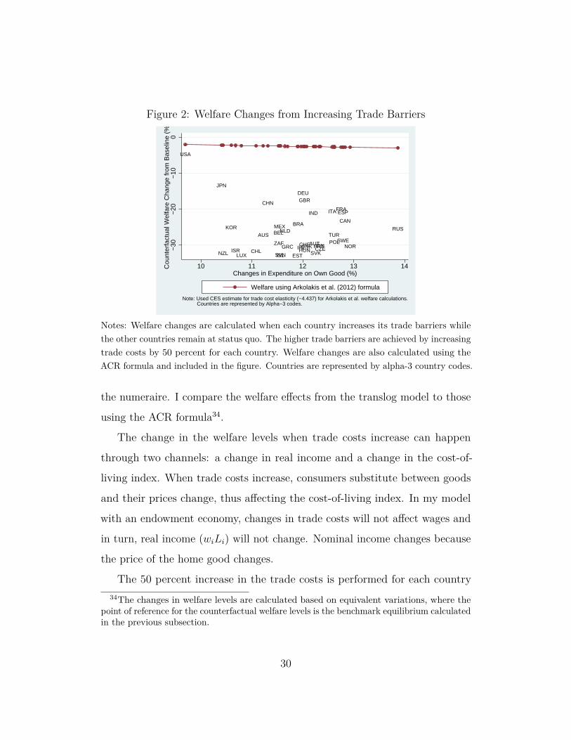
Figure 2: Welfare Changes from Increasing Trade Barriers
USA
JPN
NZL
KOR
ISRLUX
CHL
AUS
CHN
BEL
ZAF
MEX
ISLSVN
NLD
GRC
EST
BRA
IRL
DEUGBR
HUNCHEDNK
IND
AUT
SVKPRTFINCZE
ITA
TURPOL
FRAESP
SWE
CAN
NOR
RUS
−30
−20
−10
0C
ount
erfa
ctua
l Wel
fare
Cha
nge
from
Bas
elin
e (%
)
10 11 12 13 14Changes in Expenditure on Own Good (%)
Welfare using Arkolakis et al. (2012) formula
Note: Used CES estimate for trade cost elasticity (−4.437) for Arkolakis et al. welfare calculations. Countries are represented by Alpha−3 codes.
Notes: Welfare changes are calculated when each country increases its trade barriers whilethe other countries remain at status quo. The higher trade barriers are achieved by increasingtrade costs by 50 percent for each country. Welfare changes are also calculated using theACR formula and included in the figure. Countries are represented by alpha-3 country codes.
the numeraire. I compare the welfare effects from the translog model to those
using the ACR formula34.
The change in the welfare levels when trade costs increase can happen
through two channels: a change in real income and a change in the cost-of-
living index. When trade costs increase, consumers substitute between goods
and their prices change, thus affecting the cost-of-living index. In my model
with an endowment economy, changes in trade costs will not affect wages and
in turn, real income (wiLi) will not change. Nominal income changes because
the price of the home good changes.
The 50 percent increase in the trade costs is performed for each country34The changes in welfare levels are calculated based on equivalent variations, where the
point of reference for the counterfactual welfare levels is the benchmark equilibrium calculatedin the previous subsection.
30

separately, while keeping the other countries at status quo. The changes to
welfare levels are plotted in Figure 2 for brevity but all the counterfactual
results, together with the changes to the cost of living and income, are presented
in Table A.1 in the appendix. The changes to the welfare levels are significant
at the one percent level. A rise in protectionism has a varied impact on the
welfare of countries: welfare losses range from a small 4.8 percent decrease in
welfare for the U.S. to a large 32.8 percent decrease for Iceland. The variation
in the welfare losses can be explained by the expenditure on the home goods,
which recalls the welfare result in Arkolakis et al. (2012). The home good
expenditure is influenced by the size of the country and its weight in the
expenditure function.
Country size is negatively related to the welfare loss from higher trade
barriers. Small countries like Estonia, Iceland, Luxembourg, Slovak Republic,
and Slovenia suffer the largest welfare losses, while large countries like China,
Germany, Japan, the United Kingdom, and the U.S. suffer the smallest welfare
losses. This is because country size is indicative of whether the country needs
to continue importing even after increasing its barriers. When imports become
more expensive, consumers substitute to their home goods. But small countries
are less likely to have suitable substitutes to the imports, and are more likely
to continue to consume imports. The expensive imports will push up the
cost-of-living index and decrease the welfare levels of the country.
Conversely, welfare losses are mitigated by the importance of a country’s
good in the expenditure function, which is determined by αn. We can see
in Table 2 that the U.S. has the largest weight, followed by Japan, then
China. A large weight means that the good has a large demand compared to
other goods. When the importing country increases its trade barriers, local
consumers substitute to the home good, which pushes up the price of the
31

home goods. If the country has a large weight, other countries will continue
demanding this good despite the higher price, further driving up the prices.
The higher domestic prices increase nominal income, and this will dampen the
welfare losses from higher trade barriers. For example, Japan experience a large
increase of 3.47 percent in nominal income but a small welfare loss of 13.41
percent. In contrast, Estonia has a small weight in the expenditure function,
and subsequently a smaller increase in nominal income and the largest decrease
in welfare levels.
The changes in the welfare levels are plotted against the changes in the
expenditure on home goods in Figure 2. We can see that changes in welfare
levels and expenditure on home good are not linearly related. As a comparison,
welfare changes are calculated according to the ACR formula using the CES
estimate of the own-price elasticity, and represented by the line in Figure 235.
The counterfactual welfare calculations are heterogeneous and do not exhibit
any linear relationship with changes to home good expenditure. These welfare
calculations contrast sharply with those calculated with the ACR formula,
which exhibit little variation and have a strict linear relationship with changes
in home good expenditure.
The range of the welfare losses also differ vastly between the counterfactual
calculations and the ACR formula. While home good expenditure increased
between 10 to 14 percent, the variation in welfare calculations from the formula
is small: the average welfare loss is 2.6 percent with a minimum loss of 2.1
percent and a maximum loss of 3.0 percent. In contrast, the counterfactual
welfare losses are larger and more heterogeneous: the average welfare loss in the
translog model is 27 percent with a minimum loss of 4.75 and a maximum loss35Since the ACR formula summarizes the welfare changes in Novy (2013), these welfare
calculations can also be thought of as counterfactual calculations in that model.
32

of 33 percent. Compared to the translog model, the welfare losses according
to the ACR formula are eight times smaller for China, France, India, and the
U.K., and ten times smaller for Australia, Brazil, Canada and Russia.
The large difference in welfare losses between the CES and translog models is
due to the varied trade responses through the bilateral substitution elasticities
in the translog model36. In the CES model, an increase in the price of a
good causes the consumer to substitute away from that good and spread
the extra income evenly across all other goods. In the translog model, the
varying substitution elasticities mean that the consumer will not spread the
extra income evenly. On average, the substitution elasticities in the translog
model are smaller in magnitude, i.e. the bilateral trade relationships are
relatively more inelastic, compared to the CES model. The inelastic trade
relationships ensure that the country continues to import certain goods even
after the increase in import barriers. As a result, the country’s costs of living
is higher, and welfare levels lower. The importer-specific trade elasticities in
the translog model also creates the heterogeneous welfare losses. Without a
constant elasticity of substitution, welfare changes in the translog model cannot
be summarized by one sufficient statistic.
5.3 Counterfactual Analysis 2: Behind the Great Wall
For the second counterfactual analysis, I propose a scenario where China is
removed from the world trade system. China’s participation in the world
markets has reshaped international trade and more importantly, has raised36This result is supported by Ossa (2012) who finds that the welfare effects in trade models
are amplified if industry dimensions of trade flows are taken into account. He finds thatcertain imports are more important to an economy and losing access to them will mean alarger welfare loss. This is analogous to the translog model where certain trade flows aremore important to a country and when trade barriers are increased, the welfare losses willbe higher.
33

the income and welfare of its citizens and its trading partners. The effects
of China’s participation were amplified by China’s accession into the World
Trade Organization (WTO). It is therefore revealing to examine the effects of
removing China from world markets.
China’s autarkic state is achieved by increasing the bilateral distance of
China and the world by 100 times (i.e. dist′i,China = disti,China × 100 ∀i 6=
China and dist′China,j = distChina,j × 100 ∀j 6= China)37. Any trade with
China will occur at a high cost.
As expected China suffers the most when it stops trading; its welfare level
drops by 61 percent38. China has to produce its own goods when it stops trading
with the world. Chinese consumers will decrease their demand for expensive
imports and substitute to the home good. Thus, China’s consumption of its
own goods increases by 69 percent, which puts an upward pressure on domestic
prices and increases the cost of living. The large increase in the cost of living
is a major reason why China experiences such a large welfare loss. Clearly it is
not in China’s interest to retreat from the world.
Welfare levels will fall for all countries when a major manufacturing country
like China retreats from the world trading system. China’s trade partners
suffer a welfare loss of around 0.5 percent, with China’s regional trade partners
(Australia, Japan, Korea, India and New Zealand) experiencing a larger drop
in their welfare levels of around 1-2 percent. The changes to welfare levels of
China’s trade partners are plotted in Figure 3. These welfare losses are small
and they indicate that even though countries might suffer welfare loss from
not trading with China, the consequences are not catastrophic.37The usual approach of setting the bilateral distance with China to infinity is not taken
because this causes infeasibility in the model.38Table A.2 in the appendix contains the changes to the welfare levels and China’s imports
from its partners.
34

Figure 3: Welfare Losses when China stops Trading
AUS
AUT
BEL
BRA CAN
CHE
CHL
CZE
DEU
DNK
ESP
EST FIN
FRAGBR
GRCHUN
IND
IRL
ISLISR
ITA
JPN
KOR
LUX
MEX
NLD
NOR
NZL
POLPRT
RUS
SVKSVNSWE
TUR
USA
ZAF
−2
−1.
5−
1−
.50
Cou
nter
fact
ual W
elfa
re C
hang
e fr
om B
asel
ine
(%)
.22 .24 .26 .28 .3 .32Changes in Expenditure on Own Good (%)
Welfare using Arkolakis et al. (2012) formula
Note: Used CES estimate for trade cost elasticity (−4.437) for Arkolakis et al. welfare calculations. Countries are represented by Alpha−3 codes. China’s welfare level is excluded.
Notes: Welfare changes are calculated for all countries, except China, when China stopstrading with the world. This is achieved by increasing the cost of importing from andexporting to China by 100 times. Welfare changes are also calculated using the ACR formulaand included in the figure. Countries are represented by their alpha-3 country codes.
The responses of China’s trade partners to the higher trade barriers are
captured by their respective own-price elasticity, as shown in Figure 1. Iceland,
Ireland, Portugal, Spain, and United Kingdom, at the bottom left corner of the
figure, have the most elastic trade relationships with China. These countries
suffered the largest decrease of more than 300 percent in their trade with China.
Conversely, countries at the right of the figure like Australia, Korea, Japan and
New Zealand have relatively inelastic trade relationships and China did not
decrease its imports from these countries compared to other countries. As the
counterfactual simulation does not put China fully into autarky, China still
trades with some countries, which suggests that the goods from these countries
are not as substitutable as the other goods.
Welfare losses are also calculated with the ACR formula using the CES
35

elasticity estimate. Aside from China, the welfare losses from the counterfactual
analysis and the welfare formula are plotted in Figure 3 against the changes in
the expenditure on home goods. The welfare calculations from the counterfactual
analysis are more heterogeneous than those from the ACR formula. They also
do not display a clear linear relationship with changes in the expenditure on
home goods. It is noteworthy that the ACR welfare calculations underestimate
the welfare losses, which may trivialize the withdrawal of China from the
trading system.
6 Conclusion
The gravity model has been instrumental in helping us measure the size of
the gains from trade. But the theoretical models that motivate the gravity
model are single parameter models that might not be realistic in capturing
trade responses. This paper adopts a different approach by augmenting a
standard gravity model with the more flexible translog expenditure function.
It breaks the link between the own-price and cross-price elasticities, while also
giving us a unique elasticity for each bilateral pair. I apply the translog gravity
model to international trade flows among OECD and BRICS countries. The
average own-price elasticity is similar to the estimate in the CES model, but
the average substitution elasticity is lower than the CES estimate.
I estimate the model using an MPEC approach that imposes theory
consistent general equilibrium restrictions on the estimation. The model,
once calibrated via structural estimation, is used in two counterfactual analyses.
First, trade barriers for each country are raised. Every country experiences a
welfare loss when it raises its trade barriers, but the welfare loss ranges from
four to 30 percent. Countries with large manufacturing bases and weights in
the expenditure function suffer smaller welfare losses. Second, China is removed
36

from the trading system and it suffers the largest welfare loss. Even though
China is an important player in the global trading system, its removal from
the trading system decreases the welfare of most countries by only one percent.
In these counterfactual simulations, the welfare changes do not have a
linear relationship with changes in a country’s openness as implied by the
ACR formula; the welfare changes are larger and heterogeneous. The ACR
formula applies to a class of models that summarize trade responses via a single
parameter. Once we allow elasticities to vary across importers, which are more
representative of the data, the formula is no longer a good measure of welfare.
This paper complements the work by Melitz and Ottaviano (2008), Feenstra
and Weinstein (2010), and Novy (2013) in the search for an alternative to the
CES preferences. Once we move away from a single parameter model, we can
produce richer results that are a closer match to the stylized facts. This paper
adopted a more flexible demand system with a simple Armington assumption
on the supply side. Future work can enrich the flexible demand system with
richer supply-side details in the trade model.
ReferencesAnderson, James E., “A Theoretical Foundation for the Gravity Equation,” American
Economic Review, 1979, 69, 106–116.
and Eric Van Wincoop, “Gravity with Gravitas: A Solution to the Border Puzzle,”American Economic Review, 2003, 93 (1), 170–192.
and Eric van Wincoop, “Trade Costs,” Journal of Economic Literature, 2004, 42 (3),6911–751.
Arkolakis, Costas, Arnaud Costinot, and Andrés Rodriguez-Clare, “Gains fromTrade Under Monopolistic Competition: A Simple Example with Translog ExpenditureFunctions and Pareto Distributions of Firm-level Productivity,” Mimeo. MIT, 2010.
, , and , “New Trade Models, Same Old Gains?,” American Economic Review, 2012,102, 94–130.
37

Armington, Paul S., “A Theory of Demand for Products Differentiated by Place ofProduction,” International Monetary Fund Staff Papers, 1969, 16, 159–178.
Baier, Scott L. and Jeffrey H. Bergstrand, “Bonus Vetus OLS: A Simple Method forApproximating International Trade-cost Effects Using the Gravity Equation,” Journal ofInternational Economics, 2009, 77, 77–85.
Balistreri, Edward J. and Russell H. Hillberry, “Structural Estimation and the BorderPuzzle,” Journal of International Economics, 2007, 72, 451–463.
and , “The Gravity Model: An Illustration of Structural Estimation as Calibration,”Economic Inquiry, 2008, pp. 511–527.
, , and Thomas F. Rutherford, “Structural Estimation and Solution of InternationalTrade Models with Heterogeneous Firms,” Journal of International Economics, 2011, 83,95–108.
Bergstrand, Jeffrey H., “The Gravity Equation in International Trade: SomeMicroeconomic Foundations and Empirical Evidence,” Review of Economics and Statistics,1985, 67, 474–481.
, “The Generalized Gravity Equation, Monopolistic Competition, and Factor-proportionsTheory in International Trade,” Review of Economics and Statistics, 1989, 71, 143–153.
Berndt, Ernst R., The Practice of Econometrics: Classic and Contemporary, Addison-Wesley, 1991.
Chaney, Thomas, “Distorted gravity: the intensive and extensive margins of internationaltrade,” The American Economic Review, 2008, 98 (4), 1707–1721.
Deardorff, Alan V., Determinants of Bilateral Trade: Does Gravity Work in a NeoclassicalWorld?, Chicago, Il: University of Chicago Press,
Diewert, W. E. and T. J. Wales, “Flexible Function Forms and the Global CurvatureConditions,” Econometrica, 1987, 55, 43–68.
Diewert, W. Erwin, “Exact and Superlative Index Numbers,” Journal of Econometrics,1976, 4, 115–45.
Diewert, W.E. and T.J. Wales, “A Normalized Quadratic Semiflexible Functional Form,”Journal of Econometrics, 1988, 37 (3), 327–342.
38

Dornbusch, R., S. Fischer, and P. A. Samuelson, “Comparative Advantage, Trade,and Payments in a Ricardian Model with a Continuum of Goods,” American EconomicReview, 1977, 67, 823–839.
Eaton, Jonathan and Samuel Kortum, “Technology, Geography, and Trade,”Econometrica, 2002, 70 (5), 1741–1779.
Edmond, Chris, Virgiliu Midrigan, and Daniel Yi Xu, “Competition, Markups, andthe Gains from International Trade,” NBER Working Paper, 2012, No. 5515.
Feenstra, Robert C., “A Homothetic Utility Function for Monopolistic CompetitionModels, Without Constant Price Elasticity,” Economics Letters, 2003, 78, 79–86.
, “Measuring the Gains from Trade under Monopolistic Competition,” Canadian Journalof Economics, 2010, 43, 1–28.
and David E. Weinstein, “Globalization, Markups, and the U.S. Price Level,” NBERWorking Paper, 2010, No. 15749.
Haveman, Jon and David Hummels, “Alternative Hypotheses and the Volume of Trade:The Gravity Equation and the Extent of Specialization,” Canadian Journal Of Economics,2004, 37, 199–218.
Helpman, Elhanan, Marc J. Melitz, and Yona Rubinstein, “Estimating Trade Flows:Trading Partners and Trading Volumes,” Quarterly Journal of Economics, 2008, 123 (2),441–487.
Hummels, David, “Toward a Geography of Trade Costs,” Mimeo. Purdue University, 2001.
Imbs, Jean and Isabelle Mèjean, “Trade Elasticities,” Mimeo. Paris School of Economics,2011.
Judd, Kenneth L. and Che-Lin Su, “Constrained Optimization Approaches toEstimation of Structural Models,” Econometrica, 2012, 80, 2213—-2230.
Kee, Hiau Looi, Alessandro Nicita, and Marcelo Olarreaga, “Import DemandElasticities and Trade Distortion,” Review of Economics and Statistics, 2008, 90, 666–682.
Kohli, Ulrich, “Canadian Imports and Exports by Origin and Destination: A Semi-flexibleApproach,” Canadian Journal of Economics, 1994, 27, 580–603.
39

Krugman, Paul, “Scale Economies, Product Differentiation, and the Pattern of Trade,”American Economic Review, 1980, 70, 950–959.
Melitz, Marc J., “The Impact of Trade on Intra-industry Reallocations and AggregateIndustry Productivity,” Econometrica, 2003, 71 (6), 1695–1725.
and Gianmarco P. Ottaviano, “Market Size, Trade and Productivity,” Review ofEconomic Studies, 2008, 75, 295–316.
Neary, J.P., “Rationalizing the Penn World Table: True Multilateral Indices forInternational Comparisons of Real Income,” American Economic Review, 2004, pp. 1411–1428.
Novy, Dennis, “International Trade and Monopolistic Competition Without CES:Estimating Translog Gravity,” Journal of International Economics, 2013, 89, 271–282.
Ossa, Ralph, “Why Trade Matters After All,” NBER Working Paper, 2012, No. 18113.
Ryan, David L. and Terence J. Wales, “Imposing Local Concavity in the Translog andGeneralized Leontief Cost Functions,” Economics Letters, 2000, 67, 253–260.
Santos Silva, J. M. C. and Silvana Tenreyro, “The Log of Gravity,” Review ofEconomics and Statistics, 2006, 88 (4), 641–658.
Data Appendix
Nominal GDP: World Bank’s World Development Indicators (WDI).
Distances: CEPII gravity data set. Distances are measured as the population
weighted average of distance of the largest cities between countries. Distances are
normalized by the shortest distance pair (Luxembourg-Luxembourg).
Home Consumption: = 1 if importing country consumes its own good.
Aggregate Bilateral Trade: values reported to the UN COMTRADE system.
Import flows are used but if missing, they are supplemented with export flows
reported by sending country. A country’s own trade flow, not reported in the data, is
assumed to be the difference between its GDP and the total exports to all countries
in UN COMTRADE. The service component of home consumption is removed using
the ratio of service in the GDP, taken from the World Development Indicators.
40
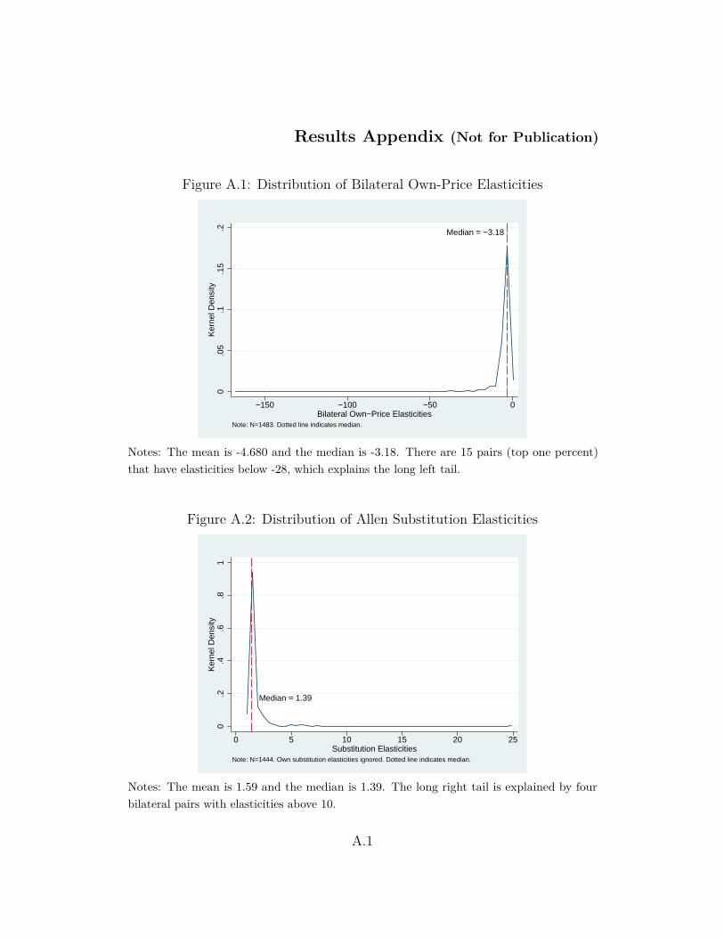
Results Appendix (Not for Publication)
Figure A.1: Distribution of Bilateral Own-Price Elasticities
Median = −3.18
0.0
5.1
.15
.2K
erne
l Den
sity
−150 −100 −50 0Bilateral Own−Price Elasticities
Note: N=1483. Dotted line indicates median.
Notes: The mean is -4.680 and the median is -3.18. There are 15 pairs (top one percent)that have elasticities below -28, which explains the long left tail.
Figure A.2: Distribution of Allen Substitution Elasticities
Median = 1.39
0.2
.4.6
.81
Ker
nel D
ensi
ty
0 5 10 15 20 25Substitution Elasticities
Note: N=1444. Own substitution elasticities ignored. Dotted line indicates median.
Notes: The mean is 1.59 and the median is 1.39. The long right tail is explained by fourbilateral pairs with elasticities above 10.
A.1

TableA.1:Rising
Protectio
nism
:Cha
nges
toWelfare,Incom
ean
dCostof
Living
Percentag
eCha
nge(%
)PercentageCha
nge(%
)PercentageCha
nge(%
)
Cou
ntry
Welfare
Costof
Living
Nom
inal
Income
Cou
ntry
Welfare
Costof
Living
Nom
inal
Income
Cou
ntry
Welfare
Costof
Living
Nom
inal
Income
Australia
-27.17
37.30
0.66
Greece
-30.44
44.12
0.25
Norway
-30.33
43.91
0.26
(1.25)
(2.32)
(0.30)
(0.54)
(1.12)
(0.12)
(0.62)
(1.27)
(0.13)
Austria
-29.55
42.55
0.43
Hun
gary
-31.40
46.07
0.20
Polan
d-29.15
41.79
0.46
(0.65)
(1.31)
(0.22)
(0.35)
(0.74)
(0.20)
(0.73)
(1.45)
(0.23)
Belgium
-26.55
37.29
0.83
Icelan
d-32.83
48.91
0.02
Portugal
-30.33
43.87
0.23
(1.02)
(1.91)
(0.83)
(0.09)
(0.20)
(0.01)
(0.55)
(1.13)
(0.00)
Brazil
-24.12
32.93
0.86
India
-21.07
28.06
1.08
Russia
-25.46
35.13
0.73
(2.04)
(3.54)
(0.00)
(1.96)
(3.27)
(0.00)
(1.55)
(2.79)
(0.36)
Can
ada
-23.26
32.15
1.41
Irelan
d-30.66
44.53
0.22
Slovak
Rep
-32.19
47.65
0.12
(2.65)
(4.65)
(0.71)
(0.45)
(0.94)
(0.11)
(0.21)
(0.46)
(0.12)
Chile
-31.68
46.58
0.14
Israel
-31.47
46.11
0.13
Slovenia
-32.71
48.70
0.06
(0.41)
(0.88)
(0.07)
(0.39)
(0.82)
(0.00)
(0.11)
(0.25)
(0.06)
China
-18.30
25.79
2.77
Italy
-20.64
28.27
1.79
SouthAfrica
-29.47
42.14
0.24
(2.51)
(3.85)
(0.00)
(1.73)
(2.79)
(0.90)
(1.14)
(2.28)
(0.12)
Czech
Rep
-31.03
45.37
0.26
Japa
n-13.41
19.49
3.47
Spain
-20.87
28.15
1.40
(0.41)
(0.86)
(0.26)
(2.02)
(2.80)
(0.00)
(1.60)
(2.60)
(0.70)
Denmark
-30.39
44.08
0.30
Korea
-25.08
34.77
0.97
Sweden
-28.70
40.89
0.45
(0.53)
(1.09)
(0.15)
(1.48)
(2.65)
(0.48)
(0.85)
(1.67)
(0.00)
Eston
ia-32.92
49.12
0.03
Luxembo
urg
-32.82
48.94
0.05
Switzerlan
d-29.83
43.08
0.40
(0.09)
(0.19)
(0.02)
(0.09)
(0.19)
(0.00)
(0.77)
(1.58)
(0.20)
Finland
-30.19
43.61
0.25
Mexico
-24.81
34.55
1.17
Turkey
-27.16
38.10
0.59
(0.63)
(1.29)
(0.25)
(1.77)
(3.18)
(0.58)
(1.13)
(2.14)
(0.30)
Fran
ce-20.01
27.51
2.00
Netherlan
ds-26.03
36.42
0.91
UnitedKingd
om-17.52
24.02
2.29
(1.91)
(3.07)
(4.99)
(1.08)
(1.99)
(0.45)
(1.92)
(2.94)
(1.15)
German
y-15.52
22.30
3.32
New
Zealan
d-32.23
47.71
0.11
UnitedStates
-4.75
15.98
(1.04)
(1.53)
(9.96)
(0.24)
(0.52)
(0.05)
(0.98)
(1.20)
Notes:Percentag
echan
gesarecalculated
asx′ x−
1wherex
′istheou
tcom
ewhentrad
ecost,τ
ij∀i6=j,
increasesby
150%
,and
xistheba
selin
ean
dthis
isdo
neforeach
coun
try.
Costof
livingis
measuredas
thepriceof
oneun
itof
welfare.U.S.f.o.b.ou
tput
isthenu
meraire
sothechan
geto
itsou
tput
is
zero.Boo
tstrap
pedstan
dard
errors
arein
parenthe
ses.
Allcoun
terfactual
resultsforchan
gesto
welfare
levels
andcost-of-livingaresign
ificant
attheon
e
percentlevel.Mostcoun
terfactual
resultsforreal
incomechan
gesaresign
ificant
atthefiv
epe
rcentlevel,except
forCzech
Repub
lic,E
ston
ia,F
inland
,
Fran
ce,G
erman
y,Hun
gary,S
lovakRepub
lican
dSo
lvenia.
A.2

TableA.2:Cha
nges
toWelfare
andIm
ports:
China
Behind
aGreat
Wall
Percentag
eCha
nge(%
)PercentageCha
nge(%
)PercentageCha
nge(%
)
Cou
ntry
Welfare
China
’sIm
ports
Cou
ntry
Welfare
China
’sIm
ports
Cou
ntry
Welfare
China
’sIm
ports
China
-60.79
68.62
Greece
-0.59
-73.51
Norway
-0.51
-113.93
(0.082
)(0.147
)(0.0006)
(0.177)
(0.0007)
(0.365)
Australia
-1.27
-25.37
Hun
gary
-0.47
-83.92
Polan
d-0.43
-84.58
(0.000
8)(0.072
)(0.0007)
(0.220)
(0.0007)
(0.223)
Austria
-0.36
-94.50
Icelan
d-0.68
-270.22
Portugal
-0.45
-214.47
(0.001
)(0.265
)(0.001)
(1.379)
(0.0007)
(0.928)
Belgium
-0.18
-141.68
India
-1.17
-28.56
Russia
-0.81
-48.53
(0.001
)(0.529
)(0.0008)
(0.064)
(0.0008)
(0.102)
Brazil
-0.57
-83.73
Irelan
d-0.40
-221.28
Slovak
Rep
-0.47
-84.78
(0.001
)(0.699
)(0.0008)
(1.004)
(0.0007)
(0.225)
Can
ada
-0.59
-66.58
Israel
-0.81
-56.10
Slovenia
-0.43
-95.51
(0.001
)(0.405
)(0.0005)
(0.123)
(0.0008)
(0.275)
Chile
-0.78
-63.35
Italy
-0.21
-104.49
SouthAfrica
-0.93
-51.46
(0.000
7)(0.370
)(0.001)
(0.305)
(0.0007)
(0.218)
Czech
Rep
-0.39
-93.87
Japa
n-1.52
-17.04
Spain
-0.22
-202.42
(0.000
8)(0.270
)(0.002)
(0.041)
(0.001)
(0.809)
Denmark
-0.40
-107
.69
Korea
-2.00
-14.55
Sweden
-0.48
-94.91
(0.000
8)(0.333
)(0.002)
(0.033)
(0.0007)
(0.272)
Eston
ia-0.67
-75.04
Luxembo
urg
-0.31
-131.63
Switzerlan
d-0.29
-123.04
(0.000
5)(0.183
)(0.0009)
(0.468)
(0.0009)
(0.457)
Finland
-0.64
-77.19
Mexico
-0.67
-51.75
Turkey
-0.63
-60.60
(0.000
6)(0.192
)(0.001)
(0.260)
(0.0007)
(0.133)
Fran
ce-0.10
-152
.36
Netherlan
ds-0.18
-136.35
UnitedKingd
om-0.07
-188.32
(0.001
)(0.569
)(0.001)
(0.485)
(0.001)
(0.888)
German
y-0.02
-113
.31
New
Zealan
d-1.29
-26.41
UnitedStates
-0.25
-51.39
(0.001
)(0.406
)(0.0007)
(0.077)
(0.002)
(0.283)
Notes:Percentag
echan
gesarecalculated
asx′ x−
1wherex
′is
theou
tcom
ewhendistan
cebe
tweenChina
anditstrad
ingpa
rtners,dist i
,Ch
inaan
d
dist C
hin
a,j
wherei,j6=China,increases
by10
000%
,and
xis
theba
selin
e.U.S.f.o.b.ou
tput
isthenu
meraire
sothechan
geto
itsou
tput
iszero.
Boo
tstrap
pedstan
dard
errors
arein
parentheses.
Allcoun
terfactual
resultsaresign
ificant
attheon
epe
rcentlevel,except
thewelfare
chan
gesforFran
ce,
German
y,Italy,
Netherlan
ds,the
U.K
.and
theU.S.
A.3