Structural Estimates of the U.S. Sacrifice Ratio

Stephen G. Cecchetti and Robert W. RichResearch and Market Analysis Group

Federal Reserve Bank of New York

March 15, 1999

We are grateful to Paul Bennett, Jordi Gali, Edward Green, Jim Kahn, Ken Kuttner, Rick Mishkinand Simon Potter for helpful comments and discussions. We would also like to thank Jordi Galiand Ken Kuttner for their assistance with programs used in performing the computations. Theviews expressed in this paper are those of the authors and do not necessarily reflect the position ofthe Federal Reserve Bank of New York or the Federal Reserve System. The authors are solelyresponsible for any remaining errors.

Structural Estimates of the U.S. Sacrifice Ratioby

Stephen G. Cecchetti and Robert W. Rich(JEL E52, C32)

Abstract -- This paper investigates the statistical properties of the U.S. sacrifice ratio -- thecumulative output loss arising from a permanent reduction in inflation. We derive estimates of thesacrifice ratio from three structural VAR models and then conduct Monte Carlo simulations toanalyze their sampling distribution. While the point estimates of the sacrifice ratio confirm theresults reported in earlier studies, we find that the estimates are very imprecise and that the degreeof imprecision increases with the complexity of the model used. That is, increases in the numberof structural shocks widen our confidence intervals. We conclude that the estimates provide avery unreliable guide for assessing the output cost of a disinflation policy.

KEY WORDS: Disinflation; Identification; Vector Autoregression; Structural shocks.

Stephen G. Cecchetti Robert W. RichDirector of Research Domestic Research FunctionFederal Reserve Bank of New York Federal Reserve Bank of New York33 Liberty Street 33 Liberty StreetNew York, NY 10045-0001 New York, NY 10045-0001(212) 720-8629 (212) 720-8100

See Barro (1996) and the collected articles in Feldstein (1999).1

As Filardo (1998) notes, the sacrifice ratio likely understates the true cost of disinflation2

because it neglects any personal costs borne by unemployed workers and their families.

1

I. Introduction

The successful conduct of monetary policy requires policymakers both to specify a set of

objectives for the performance of the economy and to understand the effects of policies designed

to attain these goals. Stabilizing prices, one of the dual goals of U.S. monetary policy, is no

different. It is generally agreed that permanently low levels of inflation create long-run benefits

for society, increasing the level and possibly the trend growth rate of real output. There is also a1

strong belief that engineering inflation reductions involve short-term costs associated with a

corresponding loss in output. Policymakers’ decisions on the timing and extent of inflation

reduction depend on a balancing of the costs and benefits of moving to a new, lower level of

inflation, which in the end requires estimates of the size of each.

The purpose of our work is to investigate the size of one aspect of this: the output cost of

disinflationary policy, usually referred to as the sacrifice ratio. The sacrifice ratio is the

cumulative loss in output, measured as a percent of one-year’s GDP, associated with a one

percentage point permanent reduction in inflation.2

While the sacrifice ratio is a key consideration for policymakers, estimating its size is a

difficult exercise, as it requires the identification of changes in the stance of monetary policy and

an evaluation of their impact on the path of output and inflation. Neither one of these

determinations is straightforward, as it is difficult to gauge the timing and extent of shifts in policy

as well as to separate the movements in output and inflation into those that were caused by policy

2

and those that were not. Finally, even if an estimate of the sacrifice ratio can be constructed, it is

critical for policymakers to know something about the precision of the estimate. It is one thing to

say that our best guess is that reducing inflation one percentage point entails a loss of 3

percentage points of GDP. But it is entirely another to go on and say that the output loss could

be anywhere from 0 to 5 or 10 percentage points of GDP.

This paper focuses on the U.S. sacrifice ratio and investigates a number of issues

associated with its construction and behavior. We examine quarterly data over the period 1959-97

and use structural vector autoregressions (SVARs) to identify shifts in monetary policy and

analyze their impact on output and inflation. Within this framework, we consider models of

increasing complexity, beginning with Cecchetti’s (1994) two-variable system, then considering

Shapiro and Watson’s (1988) three-variable system, and finally examining Gali’s (1994) four-

variable system. In each of these models, we derive estimates of the sacrifice ratio under a

different set of identifying restrictions for the structural shocks. To assess the reliability of the

sacrifice ratio estimates, we undertake a series of simulation exercises -- Monte Carlo experiments

-- that allow us to construct confidence intervals.

Our analysis generates estimates of the sacrifice ratio that vary substantially across the

models, ranging from just over 1 to nearly 10. That is, we estimate that for inflation to fall one

percentage point, somewhere between 1 and 10 percent of one year’s GDP must be sacrificed.

While the point estimates are broadly consistent with the results of previous studies, the analysis

also suggests that the sacrifice ratio is very imprecisely estimated. For example, a 90 percent

confidence interval covers zero for the point estimate in each model. Further, the sacrifice ratio

estimates display greater imprecision as the models allow for additional structural shocks. While

3

the simplest two-variable system indicates that the true value of the sacrifice ratio lies in the

interval between -0.4 and +3.2, the four-variable system suggests that the true value is somewhere

between -49 and +68. We do not take these latter estimates too literally, as the values seem

extremely implausible given our reading of the recent history. Nevertheless, they serve as a

caution to policymakers in that the point estimates would seem to provide a very unreliable guide

for gauging the output cost of a disinflation policy.

II. The Sacrifice Ratio

It is generally believed that attempts on the part of a monetary authority to lower the

inflation rate will lead to a period of increased unemployment and reduced output. The reason

why disinflationary episodes have this affect on real economic activity is because inflation displays

a great deal of persistence or inertia. That is, price inflation (measured by indices such as the

consumer price index) tends to move slowly over time, exhibiting very different behavior from

things like stock or commodity prices. Thus, the adjustment process during a disinflation requires

the monetary authority to slow aggregate demand growth, creating a period of temporary slack in

the economy that will lower the inflation rate only eventually.

A number of explanations have been offered for inflation’s slow adjustment and the

absence of costless disinflations. Fuhrer (1995) provides an overview of this discussion and

focuses on three possibilities. First, inflation persistence may arise from the overlap and non-

synchronization of wage and price contracts in the economy. Wages and prices adjust at different

times, and to each other, and so once one starts to rise, the other does too. Stopping the process

takes time. Second, people’s inflation expectations may adjust slowly over time, being based on a

See Okun (1978), Gordon and King (1982), Taylor (1983), Sargent (1983), Schelde-3

Andersen (1992) and Ball (1994).

4

sort of adaptive mechanism. Because decisions about wages and prices depend on expectations of

future changes, slow adaptation is self-fulfilling, creating inertia. And third, if people do not

believe that the monetary authority is truly committed to reducing inflation, then inflation will not

fall as rapidly. That is, the credibility of the policymaker is important in determining the dynamics

of inflation, with less credibility leading to more persistence.

The view that reductions in inflation are accompanied by a period of decreased output

(relative to trend) has generated considerable debate among economists on how to lessen the

costs of disinflation. Some discussions have focused on the speed of disinflation and whether the

monetary authority should adopt a gradualist approach or subject the economy to a “cold turkey”

remedy. Other discussions have focused on identifying the sources of inflation persistence and3

analyzing their implications for the pursuit of cost-reducing strategies.

While these theoretical discussions raise a number of important issues, the design and

implementation of disinflation policies clearly require agreement about the quantitative impact of

monetary policy on output and inflation. Measurement of the sacrifice ratio is a prerequisite to any

study attempting to evaluate its key determinants or the impact of alternative policies on the cost

of disinflation.

With this practical issue in mind, a number of authors have estimated sacrifice ratios for

the U.S. using a variety of techniques. Okun (1978) examines a family of Phillips curve models

and derives estimates that range from 6 to 18 percent of a year’s GNP, with a mean of 10 percent.

Gordon and King (1982) use traditional and vector autoregression (VAR) models to obtain

5

estimates of the sacrifice ratio that range from 0 to 8. Mankiw (1991) examines the 1982-85

Volcker disinflation and uses Okun’s law to arrive at a “back-of-the-envelope” estimate of 2.8.

More recently, Ball (1994) examines movements in trend output and trend inflation over various

disinflation episodes and obtains estimates that vary from 1.8 to 3.3.

While the estimates calculated by Ball (1994) and Mankiw (1991) are roughly the same

order of magnitude, suggesting that a consensus may exist about the size of the sacrifice ratio,

there are several remaining issues. First, prior studies do not, in our view, adequately control for

the impact of nonmonetary factors on the behavior of output and inflation. Consider the plots of

the quarterly growth rate of real GDP and the consumer price index (CPI) displayed in Figure 1.

While some of the movements in output and inflation over the post-World War II period are

surely attributable to monetary policy actions, it is unreasonable on either theoretical grounds or

from visual inspection to believe they all are. Thus, computing a meaningful estimate of the

sacrifice ratio requires more than simply calculating a measure of the association between output

and inflation during arbitrarily selected episodes. Rather, it depends critically on isolating which

movements are the result of monetary influences.

Secondly, previous studies such as Gordon and King (1982) fail to account for the policy

process. Some of the actions undertaken by a monetary authority are intended to accommodate or

offset shocks to the economy. However, the analysis of Gordon and King does not allow the

movements in a policy variable to be separated into those associated with a shift in policy and

those reflecting a systematic (or endogenous) response to the state of the economy. This type of

decomposition, which is necessary to assess the effects of monetary policy on the economy,

requires the specification and estimation of a structural economic model.

This discussion abstracts from other considerations such as Ball’s identification of4

disinflation episodes or the construction of his measures of trend output and trend inflation.

Cecchetti (1994) refers to the increase in output from a higher inflation rate as the5

“benefit ratio”. If monetary policy has symmetric effects on output an inflation, then the benefitratio and sacrifice ratio would simply be mirror images of each other.

Filardo’s results associate the moderate growth regime with a Phillips curve whose slope6

is essentially zero. Filardo does not report an estimate for the sacrifice ratio for this regimebecause the within-regime value would approach infinity.

6

Another important issue concerns the periods selected for the empirical analysis. Studies

such as Ball (1994) focus solely on specific disinflationary episodes -- periods when

contractionary monetary policy are thought to have resulted in the reduction in both inflation and

output. However, it is not obvious that estimates of the sacrifice ratio should exclude a priori

episodes in which inflation and output are both increasing. Such an approach would only be

justified if there were an accepted asymmetry in the impact of monetary policy on output and

prices. In the absence of such evidence, economic expansions would contain episodes in which4

output and inflation increased as a result of expansionary monetary policy. Such episodes would

then be as informative about the sacrifice ratio as a disinflation.5

Filardo (1998) is an exception, as he presents evidence that the sacrifice ratio for the U.S.

varies across three regimes corresponding to periods of weak, moderate and strong output

growth. Using a measure of the sacrifice ratio similar to that used in this study, Filardo derives

sacrifice ratio estimates of 5.0 in the weak growth regime and 2.1 in the strong growth regime.6

While the findings of Filardo offer new and interesting insights into the output cost of

disinflation, his study, along with previous work, is silent on the accuracy of the estimates.

Specifically, there has been no serious attempt to characterize the statistical precision of sacrifice

7

ratio measures. Estimation of economic relationships and magnitudes inherently involves some

uncertainty and it is extremely important to quantify their reliability. For example, policymakers

may be reluctant to undertake certain policy actions unless they can attach a high degree of

confidence to the predicted outcomes.

Characterizing the precision of sacrifice ratio estimates is a primary goal of our analysis.

We do this by studying the properties of three structural vector autoregression (SVAR) models.

We now turn to a discussion of the SVAR estimation methodology and a description of the

models that we use to construct sacrifice ratio estimates.

III. Structural Vector Autoregressions and Monetary Policy Shocks

The structural vector autoregression (SVAR) approach that we adopt here remains a

popular technique for analyzing the effects of monetary policy on output and prices. A SVAR can

be viewed as a dynamic simultaneous equations model with identifying restrictions based on

economic theory. In particular, the SVAR relates the observed movements in a variable to a set of

structural shocks -- innovations that are fundamental in the sense that they have an economic

interpretation. In the formulation of their identification assumptions, the models we employ appeal

to economic theories which then allow us to interpret one of the structural innovations as a

monetary policy shock. For this reason, we find the SVAR methodology attractive in evaluating

monetary policy’s impact on output and inflation, and giving us a measure of the sacrifice ratio.

The SVAR approach decomposes monetary policy into a systematic and a random

component. The systematic component can be thought of as a reaction function and describes the

historical response of the monetary authority to movements in a set of key economic variables.

(1 L)yt �yt Mn

i1

bi11�yti � b0

12�%t � Mn

i1

bi12�%ti � �

yt

(1 L)%t �%t b021�yt � M

n

i1

bi21�yti � M

n

i1

bi22�%ti � �

%

t

yt %t

�t [�yt ,�%t ]�

(�yt ) (�%t ) �t

E[�t��

t] 6

This point underscores the importance of differentiating between changes in monetary7

policy that reflect a systematic (or endogenous) response to the state of the economy and a shift inthe stance of policy. Specifically, our evaluation of the sacrifice ratio corresponds to a ‘pure’monetary tightening and does not arise as a consequence of (or as a response to) other shocks.

The SVAR approach is not without its limitations. The estimated effects of shocks can8

vary substantially as a result of slight changes in identifying restrictions. Thus, it may be quiteimportant to consider a set of models when drawing inferences based upon the SVAR approach.

The model includes the change (or first difference) of inflation which allows shocks to9

have a permanent effect on the level of inflation. The differencing of the inflation series is alsorequired to account for its nonstationary behavior over the sample period. We later discuss theresults of unit root tests for inflation and output.

8

(1)

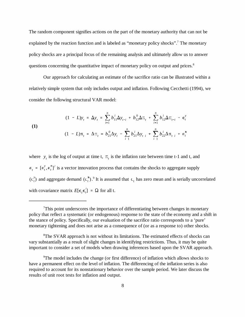
The random component signifies actions on the part of the monetary authority that can not be

explained by the reaction function and is labeled as “monetary policy shocks”. The monetary7

policy shocks are a principal focus of the remaining analysis and ultimately allow us to answer

questions concerning the quantitative impact of monetary policy on output and prices.8

Our approach for calculating an estimate of the sacrifice ratio can be illustrated within a

relatively simple system that only includes output and inflation. Following Cecchetti (1994), we

consider the following structural VAR model:

where is the log of output at time t, is the inflation rate between time t-1 and t, and

is a vector innovation process that contains the shocks to aggregate supply

and aggregate demand . It is assumed that has zero mean and is serially uncorrelated9

with covariance matrix for all t.

(1 L)yt A11(L)�yti � A12(L)�%ti M

�

i0

ai11�

yti � M

�

i0

ai12�

%

ti

(1 L)%t A21(L)�yti � A22(L)�%ti M

�

i0

ai21�

yti � M

�

i0

ai22�

%

ti

S�%(-)

M-

j0

0yt�j

0�%

t

0%t�-

0�%

t

(M0

i0

ai12) � (M

1

i0

ai12) � . . . � (M

-

i0

ai12)

(M-

i0

ai22)

(M-

i0M

i

j0

ai12)

(M-

i0

ai22)

.

Aij(L)

A22(L)

A21(L)

9

(2)

(3)

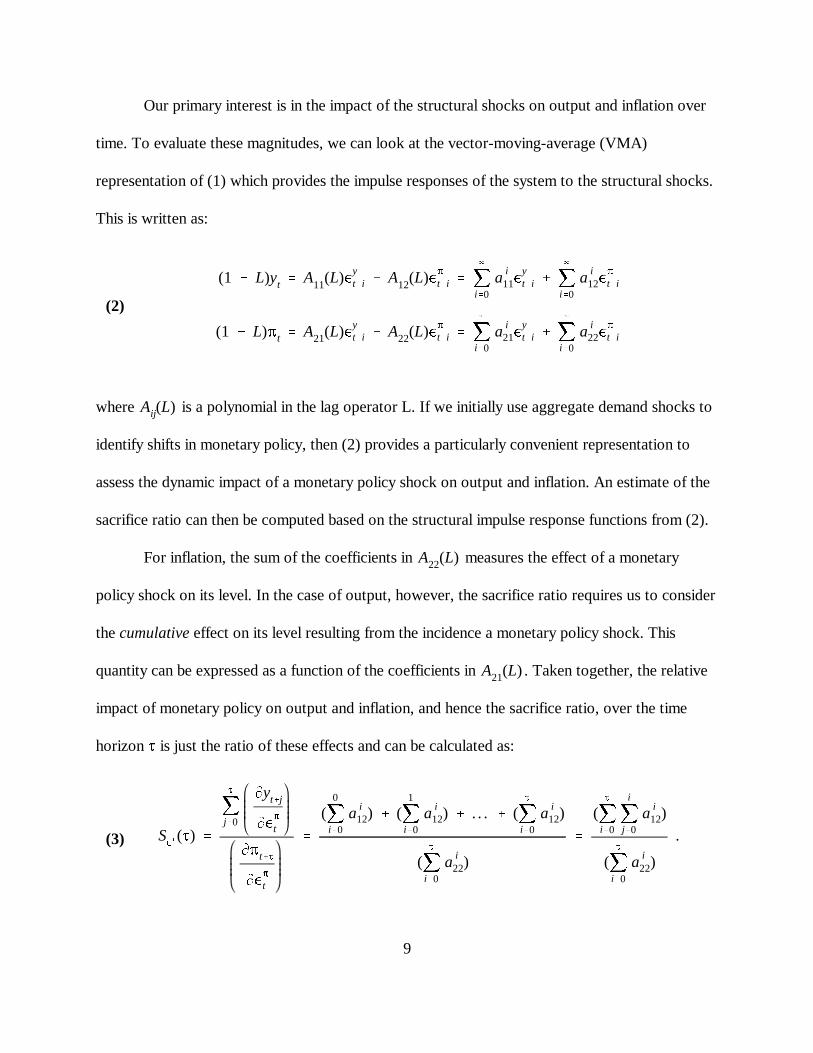
Our primary interest is in the impact of the structural shocks on output and inflation over

time. To evaluate these magnitudes, we can look at the vector-moving-average (VMA)

representation of (1) which provides the impulse responses of the system to the structural shocks.

This is written as:

where is a polynomial in the lag operator L. If we initially use aggregate demand shocks to

identify shifts in monetary policy, then (2) provides a particularly convenient representation to

assess the dynamic impact of a monetary policy shock on output and inflation. An estimate of the

sacrifice ratio can then be computed based on the structural impulse response functions from (2).

For inflation, the sum of the coefficients in measures the effect of a monetary

policy shock on its level. In the case of output, however, the sacrifice ratio requires us to consider

the cumulative effect on its level resulting from the incidence a monetary policy shock. This

quantity can be expressed as a function of the coefficients in . Taken together, the relative

impact of monetary policy on output and inflation, and hence the sacrifice ratio, over the time

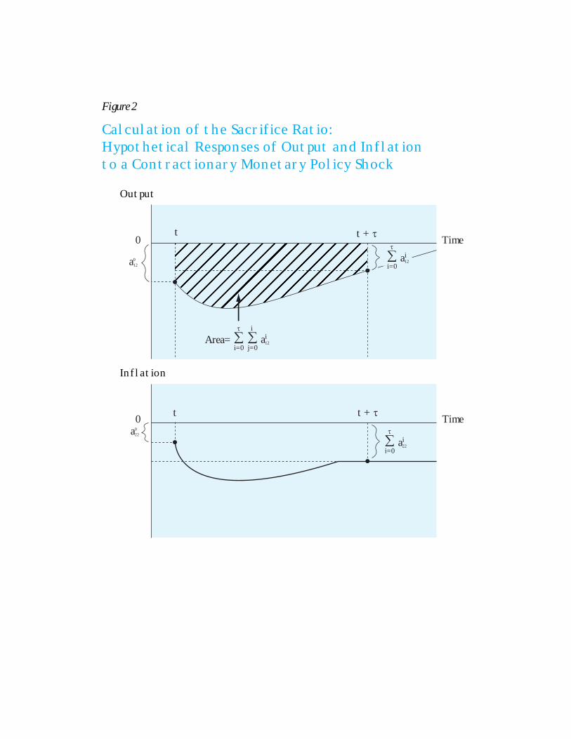
horizon - is just the ratio of these effects and can be calculated as:

6

A12(1) M�

i0

ai12 0

The numerator of the sacrifice ratio in equation (3) is calculated as the sum of the10

changes in output. A more accurate measure would take into account the timing of the outputlosses by incorporating a real interest rate and accumulating the sum of discounted changes inoutput.

The Technical Appendix provides further details on the identification of SVAR models.11

10

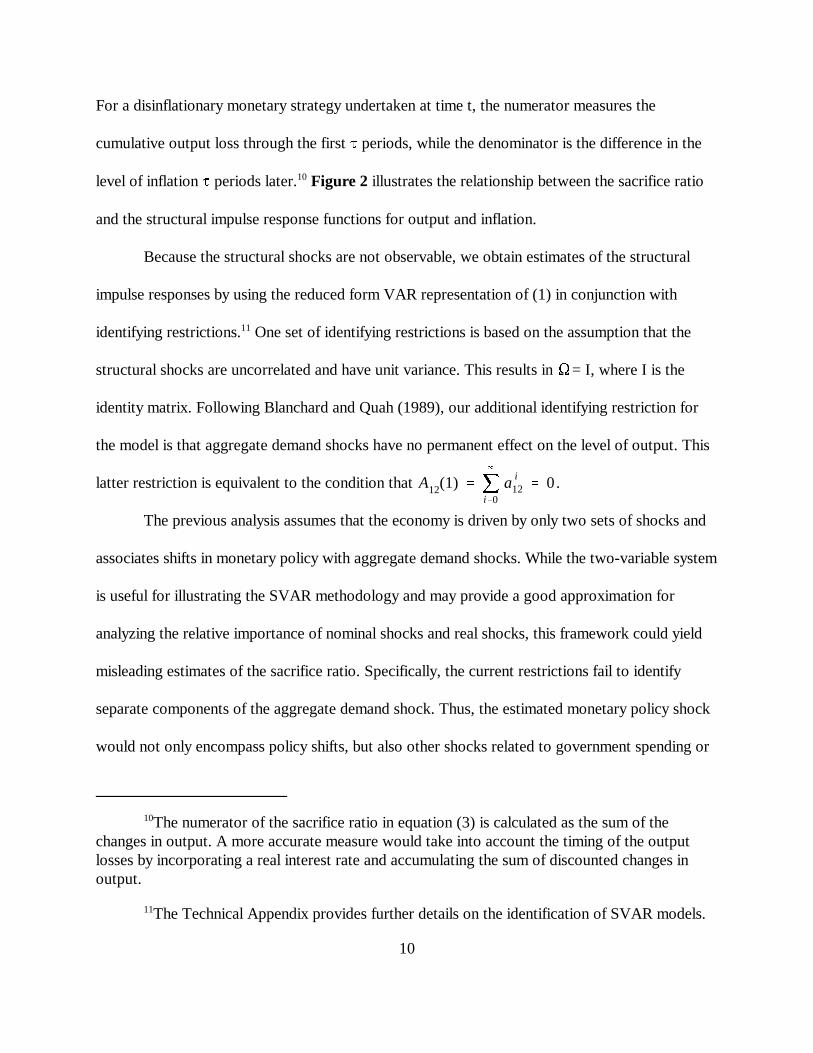
For a disinflationary monetary strategy undertaken at time t, the numerator measures the

cumulative output loss through the first - periods, while the denominator is the difference in the

level of inflation - periods later. Figure 2 illustrates the relationship between the sacrifice ratio10

and the structural impulse response functions for output and inflation.

Because the structural shocks are not observable, we obtain estimates of the structural

impulse responses by using the reduced form VAR representation of (1) in conjunction with

identifying restrictions. One set of identifying restrictions is based on the assumption that the 11

structural shocks are uncorrelated and have unit variance. This results in = I, where I is the

identity matrix. Following Blanchard and Quah (1989), our additional identifying restriction for

the model is that aggregate demand shocks have no permanent effect on the level of output. This

latter restriction is equivalent to the condition that .

The previous analysis assumes that the economy is driven by only two sets of shocks and

associates shifts in monetary policy with aggregate demand shocks. While the two-variable system

is useful for illustrating the SVAR methodology and may provide a good approximation for

analyzing the relative importance of nominal shocks and real shocks, this framework could yield

misleading estimates of the sacrifice ratio. Specifically, the current restrictions fail to identify

separate components of the aggregate demand shock. Thus, the estimated monetary policy shock

would not only encompass policy shifts, but also other shocks related to government spending or

�yt

�%t

(i t%t)

A(L)

�yt

�LMt

�ISt

i t (i t %t)

�yt

�LMt �

ISt

a012 0

While we refer to this as the “Shapiro-Watson model”, our model actually differs from12

theirs in two small ways. First, Shapiro and Watson decompose aggregate supply innovations into a technology shock and a labor supply shock. Second, they also include oil prices as an

11

(4)

shifts in consumption or investment functions.

To provide a more detailed analysis, we also derive estimates of the sacrifice ratio from

models developed by Shapiro and Watson (1988) and Gali (1992). These models allow us to

decompose the aggregate demand shock into individual components and therefore can be used to

judge the sensitivity of the results to alternative measures of the monetary policy shock.

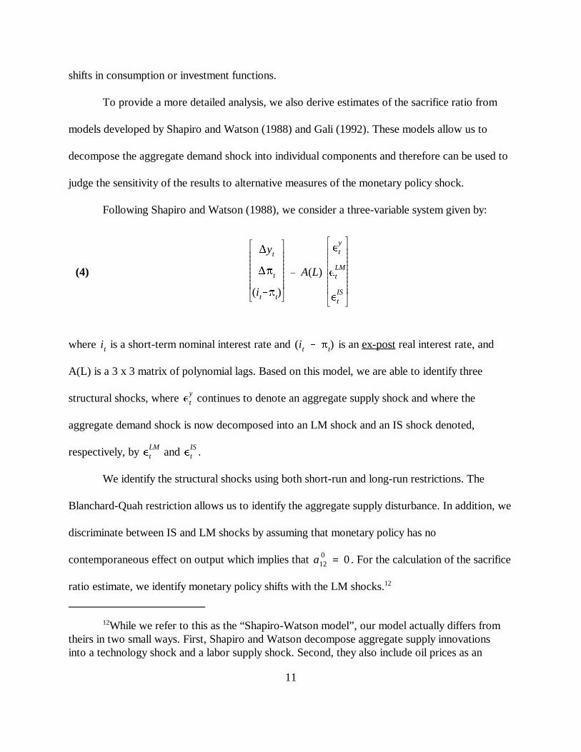
Following Shapiro and Watson (1988), we consider a three-variable system given by:

where is a short-term nominal interest rate and is an ex-post real interest rate, and

A(L) is a 3 x 3 matrix of polynomial lags. Based on this model, we are able to identify three

structural shocks, where continues to denote an aggregate supply shock and where the

aggregate demand shock is now decomposed into an LM shock and an IS shock denoted,

respectively, by and .

We identify the structural shocks using both short-run and long-run restrictions. The

Blanchard-Quah restriction allows us to identify the aggregate supply disturbance. In addition, we

discriminate between IS and LM shocks by assuming that monetary policy has no

contemporaneous effect on output which implies that . For the calculation of the sacrifice

ratio estimate, we identify monetary policy shifts with the LM shocks.12

�it (i t %t)

�yt

�i t

(i t%t)

(�mt%t)

A(L)

�yt

�MSt

�MDt

�ISt

mt (�mt %t)

�MSt , �MD

t �ISt

a012 a0

13 0

b023 � b0

24 0

exogenous regressor in their SVAR system.

Although the inflation rate does not appear as an individual variable in the Gali (1992)13

model, we can recover its impulse response function from the estimated impulse responsefunctions for and

12

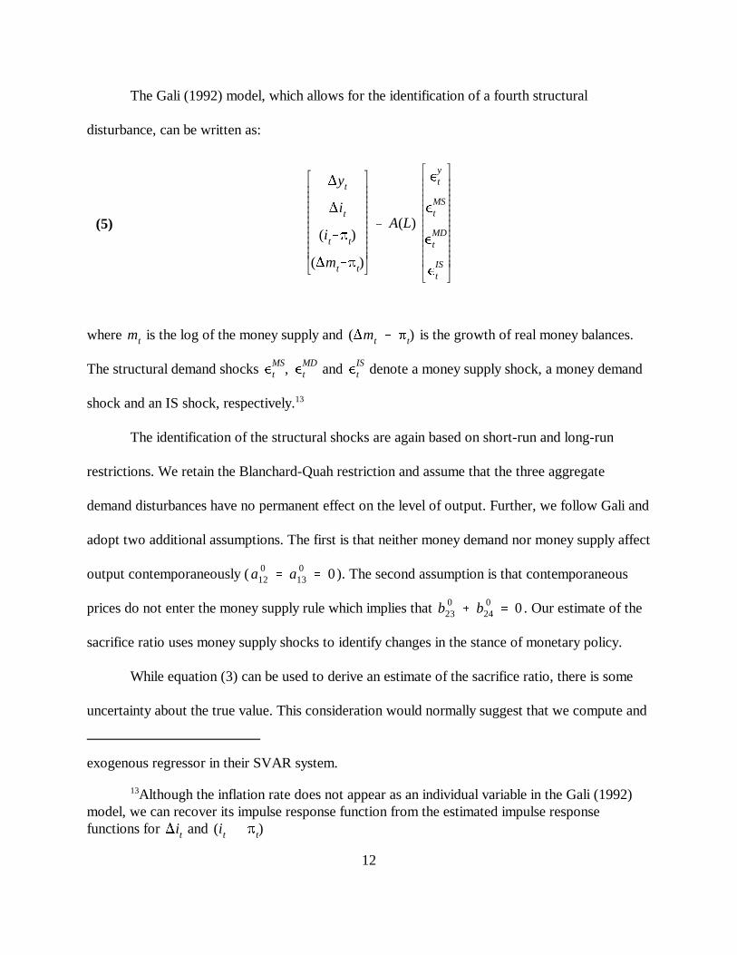
(5)

The Gali (1992) model, which allows for the identification of a fourth structural

disturbance, can be written as:

where is the log of the money supply and is the growth of real money balances.

The structural demand shocks and denote a money supply shock, a money demand

shock and an IS shock, respectively. 13

The identification of the structural shocks are again based on short-run and long-run

restrictions. We retain the Blanchard-Quah restriction and assume that the three aggregate

demand disturbances have no permanent effect on the level of output. Further, we follow Gali and

adopt two additional assumptions. The first is that neither money demand nor money supply affect

output contemporaneously ( ). The second assumption is that contemporaneous

prices do not enter the money supply rule which implies that . Our estimate of the

sacrifice ratio uses money supply shocks to identify changes in the stance of monetary policy.

While equation (3) can be used to derive an estimate of the sacrifice ratio, there is some

uncertainty about the true value. This consideration would normally suggest that we compute and

µt

S�%(-)

ai12 ai

22

� { µ1, µ2, . . . µT}

�

{ µ1, µ2, . . . µT}

The Delta method would require an estimate of the variance-covariance matrix of the14

parameters in (2) as well as the calculation of the first-derivatives of the function [equation (3)]with respect to the estimated parameter vector. However, obtaining estimates of the variance-covariance matrix of the impulse response functions is an extremely difficult task. While there aremethods that allow for such a calculation in the case of the two-variable system, the three- andfour-variable systems are too complex for these methods to be feasible. Therefore, we adopt aconsiderably easier and more tractable approach for assessing the precision of the sacrifice ratioestimates. In addition, consistency of the estimates produced by the Delta method relies on theassumption of normality which is a condition that is likely violated in the sample.

The estimated residuals denote the (n x 1) vector of innovations to the reduced form15

VAR at time t.

13

report a standard error to determine the imprecision attached to the estimate. In the case of the

sacrifice ratio, however, the calculation of a standard error is difficult, as is a function of

the parameters in the structural VMA ( the ’s and ’s). Moreover, while the application of

the Delta method might appear to offer a solution to this problem, this technique would be

computationally demanding because of complexities associated with the nature of the impulse

response functions in equation (2).14

As an alternative approach for gauging the reliability of the sacrifice ratio estimates, we

employ Monte Carlo methods. In using these techniques, our goal is to approximate the exact

sampling distribution of the estimator of the sacrifice ratio in equation (3). The approximation is

derived using a bootstrap method and involves a large number of replications. The procedure can

be briefly described as follows.

Let � denote the vector of parameters that constitute the reduced form VAR model and

let and denote, respectively, the estimated parameter vector and residuals of

the reduced form VAR using the observed set of data. The estimated parameter vector along15

with the estimated residuals can be used to generate a full sample of artificial

{ µ1, µ2, . . . µT}

S�%(-) S

�%(-) [S

�%(-) S

�%(-)]

��

1

S1(��

1) S�%(-)

S2(��

2)

S1(��

1) , S2(��

2) ,á , SN(��

N) S�%(-)

Si(�i)

S�%(-) S

�%(-)

S�%(-)

The individual observations for an artificial sample are generated by randomly drawing a16

single realization from and adding the realization to the estimated equations inthe reduced form VAR based on the historical data. The full sample of artificial data is thenconstructed by repeating this process T times, where it is assumed that the sampling of theestimated innovations takes place with replacement. Because of the presence of lagged terms inthe VAR system, the presample values of the variables are set equal to those actually observed inthe data.

14

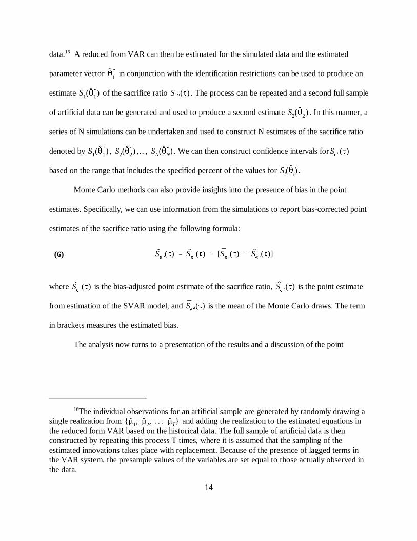
(6)

data. A reduced from VAR can then be estimated for the simulated data and the estimated16

parameter vector in conjunction with the identification restrictions can be used to produce an

estimate of the sacrifice ratio . The process can be repeated and a second full sample

of artificial data can be generated and used to produce a second estimate . In this manner, a

series of N simulations can be undertaken and used to construct N estimates of the sacrifice ratio

denoted by . We can then construct confidence intervals for

based on the range that includes the specified percent of the values for .

Monte Carlo methods can also provide insights into the presence of bias in the point

estimates. Specifically, we can use information from the simulations to report bias-corrected point

estimates of the sacrifice ratio using the following formula:

where is the bias-adjusted point estimate of the sacrifice ratio, is the point estimate

from estimation of the SVAR model, and is the mean of the Monte Carlo draws. The term

in brackets measures the estimated bias.

The analysis now turns to a presentation of the results and a discussion of the point

We restrict our attention to nonrecursive structural VAR models in this study. This17

consideration is principally based on the observation that small recursive systems can produceanomalous responses on the part of variables to a monetary policy shock. The usual practice forresolving this outcome is to include additional variables. However, this approach would limit ourability to study systems characterized by a small number of structural shocks and to analyze thesensitivity of the results to various decompositions of the aggregate demand shock.

15

estimates and their associated confidence intervals.17

IV. Empirical Results

We construct estimates of the sacrifice ratio from the three structural VAR models using

quarterly data over the sample period 1959:Q1-1997:Q4. Output is measured by real GDP and

inflation by the percentage change in the consumer price index (CPI). The short-term interest rate

represents the yield on three-month Treasury bills and the monetary aggregate is measured by M1.

The Data Appendix describes the data in further detail.

Estimation of the sacrifice ratio also requires the selection of horizons for the long-run

restriction on aggregate demand shocks and to calculate the dynamic response of output and

inflation to monetary policy shocks. Following Cecchetti (1994), we assume that aggregate

demand shocks completely die out after twenty years and compute estimates of the sacrifice ratio

based on the response of output and inflation occurring five years after a shift in monetary policy.

That is, we truncate the structural VMA representations at eighty quarters and set - equal to

twenty quarters.

It is also worth noting that preliminary analysis of the data provided support for the model

specifications. In particular, we examined the stationarity properties of the various series in order

to determine the appropriate differencing of the data. The results from the application of Dickey-

Fuller (1979) unit root tests provided evidence that the ex post real interest rate and the growth

The presence of a unit root in the output process allows the long-run restriction on the 18

effects of aggregate demand shocks to be well-defined and meaningful. As previously discussed,the presence of a unit root in the inflation process allows for permanent shifts in its level.

The lag length of the reduced form VAR was set equal to eight for the Cecchetti model19

and equal to four for the Shapiro-Watson and Gali models. The estimates of the sacrifice ratio arebased on a different transformation of the data for output and prices. Output growth is measuredat a quarterly rate in percentage terms, while inflation is measured at an annual rate in percentageterms.

Ball (1994) and Schelde-Andersen (1992) obtain estimates of 1.8 and 1.4, respectively.20

16

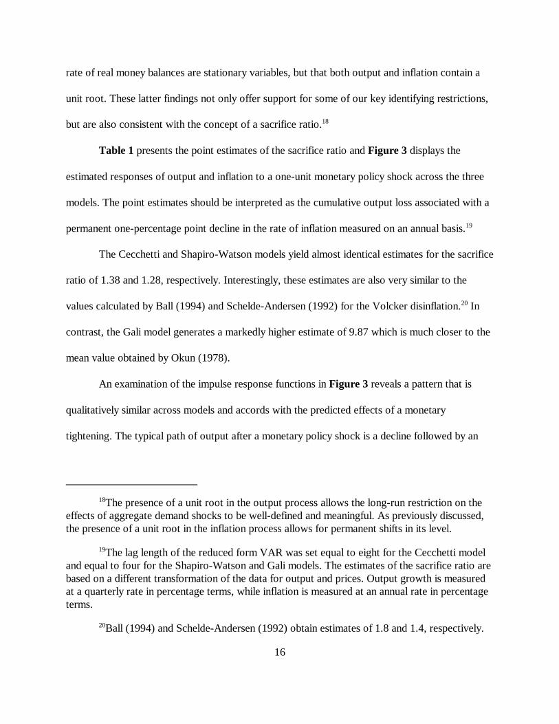
rate of real money balances are stationary variables, but that both output and inflation contain a

unit root. These latter findings not only offer support for some of our key identifying restrictions,

but are also consistent with the concept of a sacrifice ratio.18

Table 1 presents the point estimates of the sacrifice ratio and Figure 3 displays the

estimated responses of output and inflation to a one-unit monetary policy shock across the three

models. The point estimates should be interpreted as the cumulative output loss associated with a

permanent one-percentage point decline in the rate of inflation measured on an annual basis. 19

The Cecchetti and Shapiro-Watson models yield almost identical estimates for the sacrifice

ratio of 1.38 and 1.28, respectively. Interestingly, these estimates are also very similar to the

values calculated by Ball (1994) and Schelde-Andersen (1992) for the Volcker disinflation. In20

contrast, the Gali model generates a markedly higher estimate of 9.87 which is much closer to the

mean value obtained by Okun (1978).

An examination of the impulse response functions in Figure 3 reveals a pattern that is

qualitatively similar across models and accords with the predicted effects of a monetary

tightening. The typical path of output after a monetary policy shock is a decline followed by an

The nature of the identification restrictions in the Shapiro-Watson and Gali models21

precludes a contemporaneous response of output to the monetary policy shock.

For purposes of presentation, the frequency density functions only include the22

observations falling in the 2.5%-97.5% fractile range.

17

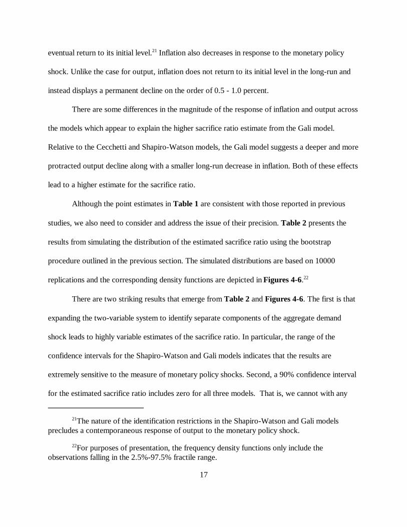
eventual return to its initial level. Inflation also decreases in response to the monetary policy21

shock. Unlike the case for output, inflation does not return to its initial level in the long-run and

instead displays a permanent decline on the order of 0.5 - 1.0 percent.

There are some differences in the magnitude of the response of inflation and output across

the models which appear to explain the higher sacrifice ratio estimate from the Gali model.

Relative to the Cecchetti and Shapiro-Watson models, the Gali model suggests a deeper and more

protracted output decline along with a smaller long-run decrease in inflation. Both of these effects

lead to a higher estimate for the sacrifice ratio.

Although the point estimates in Table 1 are consistent with those reported in previous

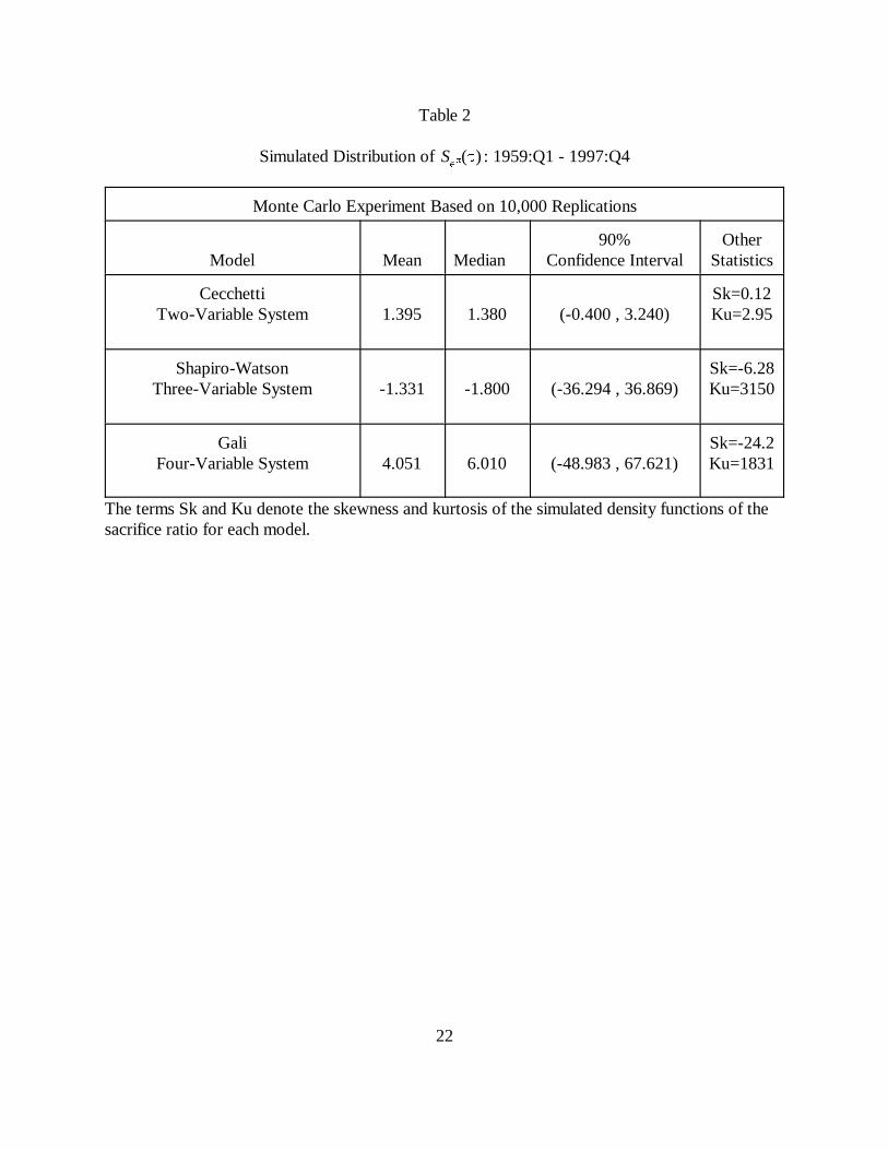
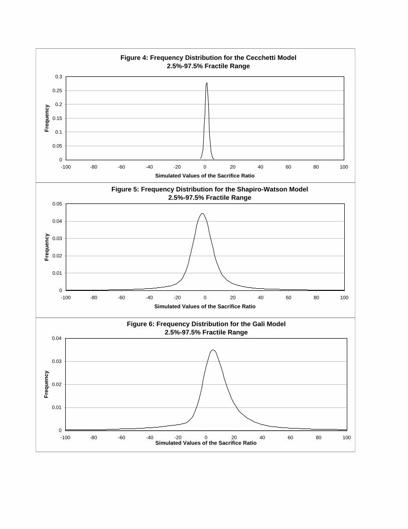
studies, we also need to consider and address the issue of their precision. Table 2 presents the

results from simulating the distribution of the estimated sacrifice ratio using the bootstrap

procedure outlined in the previous section. The simulated distributions are based on 10000

replications and the corresponding density functions are depicted in Figures 4-6.22

There are two striking results that emerge from Table 2 and Figures 4-6. The first is that

expanding the two-variable system to identify separate components of the aggregate demand

shock leads to highly variable estimates of the sacrifice ratio. In particular, the range of the

confidence intervals for the Shapiro-Watson and Gali models indicates that the results are

extremely sensitive to the measure of monetary policy shocks. Second, a 90% confidence interval

for the estimated sacrifice ratio includes zero for all three models. That is, we cannot with any

S�%(-)

The bias-corrected point estimates of the sacrifice ratio for the Shapiro-Watson and Gali23

models are 3.885 and 15.691, respectively.

18

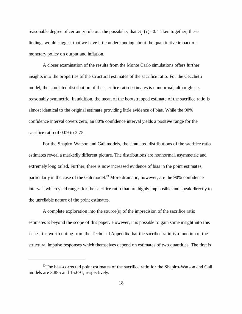
reasonable degree of certainty rule out the possibility that =0. Taken together, these

findings would suggest that we have little understanding about the quantitative impact of

monetary policy on output and inflation.

A closer examination of the results from the Monte Carlo simulations offers further

insights into the properties of the structural estimates of the sacrifice ratio. For the Cecchetti

model, the simulated distribution of the sacrifice ratio estimates is nonnormal, although it is

reasonably symmetric. In addition, the mean of the bootstrapped estimate of the sacrifice ratio is

almost identical to the original estimate providing little evidence of bias. While the 90%

confidence interval covers zero, an 80% confidence interval yields a positive range for the

sacrifice ratio of 0.09 to 2.75.

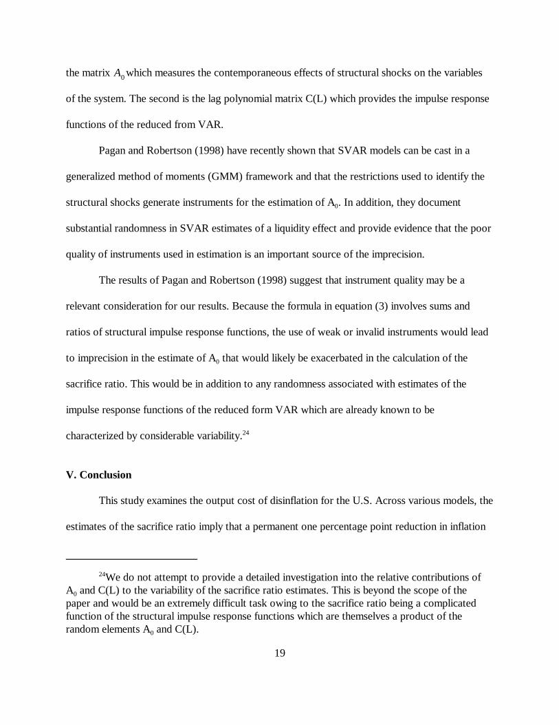
For the Shapiro-Watson and Gali models, the simulated distributions of the sacrifice ratio

estimates reveal a markedly different picture. The distributions are nonnormal, asymmetric and

extremely long tailed. Further, there is now increased evidence of bias in the point estimates,

particularly in the case of the Gali model. More dramatic, however, are the 90% confidence23

intervals which yield ranges for the sacrifice ratio that are highly implausible and speak directly to

the unreliable nature of the point estimates.

A complete exploration into the source(s) of the imprecision of the sacrifice ratio

estimates is beyond the scope of this paper. However, it is possible to gain some insight into this

issue. It is worth noting from the Technical Appendix that the sacrifice ratio is a function of the

structural impulse responses which themselves depend on estimates of two quantities. The first is

A0

We do not attempt to provide a detailed investigation into the relative contributions of24

A and C(L) to the variability of the sacrifice ratio estimates. This is beyond the scope of the0

paper and would be an extremely difficult task owing to the sacrifice ratio being a complicatedfunction of the structural impulse response functions which are themselves a product of therandom elements A and C(L).0

19

the matrix which measures the contemporaneous effects of structural shocks on the variables

of the system. The second is the lag polynomial matrix C(L) which provides the impulse response

functions of the reduced from VAR.

Pagan and Robertson (1998) have recently shown that SVAR models can be cast in a

generalized method of moments (GMM) framework and that the restrictions used to identify the

structural shocks generate instruments for the estimation of A . In addition, they document0

substantial randomness in SVAR estimates of a liquidity effect and provide evidence that the poor

quality of instruments used in estimation is an important source of the imprecision.

The results of Pagan and Robertson (1998) suggest that instrument quality may be a

relevant consideration for our results. Because the formula in equation (3) involves sums and

ratios of structural impulse response functions, the use of weak or invalid instruments would lead

to imprecision in the estimate of A that would likely be exacerbated in the calculation of the0

sacrifice ratio. This would be in addition to any randomness associated with estimates of the

impulse response functions of the reduced form VAR which are already known to be

characterized by considerable variability.24

V. Conclusion

This study examines the output cost of disinflation for the U.S. Across various models, the

estimates of the sacrifice ratio imply that a permanent one percentage point reduction in inflation

This includes both nonrecursive and recursive structural VAR models. It is also25

important to note that the imprecision of the sacrifice ratio estimates in the Shapiro-Watson modelis not due to a reduction in the degrees of freedom. Because of different lag lengths, the degreesof freedom in the Cecchetti and Shapiro-Watson models are approximately equal.

Alternative identification schemes are unlikely to change this outcome. Unlike standard 26

situations which allow for the application of instrumental variables procedures, the instrument set available for the estimation of SVAR models is very restricted. This lack of valid instruments mayimpose severe restrictions on the nature of the structural shocks that can be identified.

20

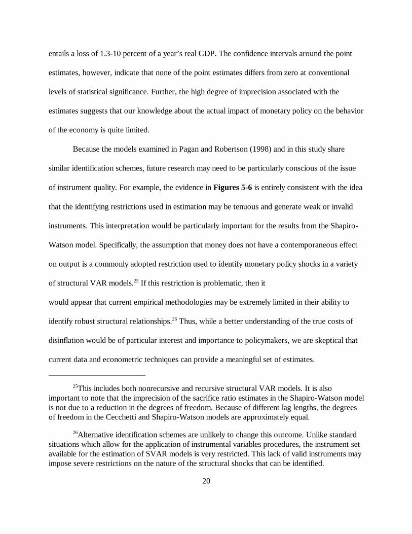
entails a loss of 1.3-10 percent of a year’s real GDP. The confidence intervals around the point

estimates, however, indicate that none of the point estimates differs from zero at conventional

levels of statistical significance. Further, the high degree of imprecision associated with the

estimates suggests that our knowledge about the actual impact of monetary policy on the behavior

of the economy is quite limited.

Because the models examined in Pagan and Robertson (1998) and in this study share

similar identification schemes, future research may need to be particularly conscious of the issue

of instrument quality. For example, the evidence in Figures 5-6 is entirely consistent with the idea

that the identifying restrictions used in estimation may be tenuous and generate weak or invalid

instruments. This interpretation would be particularly important for the results from the Shapiro-

Watson model. Specifically, the assumption that money does not have a contemporaneous effect

on output is a commonly adopted restriction used to identify monetary policy shocks in a variety

of structural VAR models. If this restriction is problematic, then it 25

would appear that current empirical methodologies may be extremely limited in their ability to

identify robust structural relationships. Thus, while a better understanding of the true costs of26

disinflation would be of particular interest and importance to policymakers, we are skeptical that

current data and econometric techniques can provide a meaningful set of estimates.

S�%(-)

21

Table 1

Estimated Sacrifice Ratio for the United States: 1959:Q1 - 1997:Q4

Cumulative 5-Year Output Loss as a Percentage of Real GDP

Model

CecchettiTwo-Variable System 1.376

Shapiro-WatsonThree-Variable System 1.277

GaliFour-Variable System 9.871

S�%(-)

22

Table 2

Simulated Distribution of : 1959:Q1 - 1997:Q4

Monte Carlo Experiment Based on 10,000 Replications

Model Mean Median Confidence Interval Statistics90% Other

Cecchetti Sk=0.12Two-Variable System 1.395 1.380 (-0.400 , 3.240) Ku=2.95

Shapiro-Watson Sk=-6.28Three-Variable System -1.331 -1.800 (-36.294 , 36.869) Ku=3150

Gali Sk=-24.2Four-Variable System 4.051 6.010 (-48.983 , 67.621) Ku=1831

The terms Sk and Ku denote the skewness and kurtosis of the simulated density functions of thesacrifice ratio for each model.

Xt D1Xt1 D2Xt2 . . . DkXtk D(L)Xt µt , E[µ tµ�

t ] ( ~ t

Xt µt � C1µt1 � C2µt2 � . . . C(L)µt

B0Xt B1Xt1 � B2Xt2 � . . . � BkXtk � �t, E[�t��

t ] 6 ~ t

Xt A0�t � A1�t1 � . . . A(L)�t

E[(A0�)(A0�)� ] A06A �

0 ( E[(µ)(µ� )]

Xt

µt

23

(A.1)

(A.2)

(A.3)

(A.4)

(A.5)

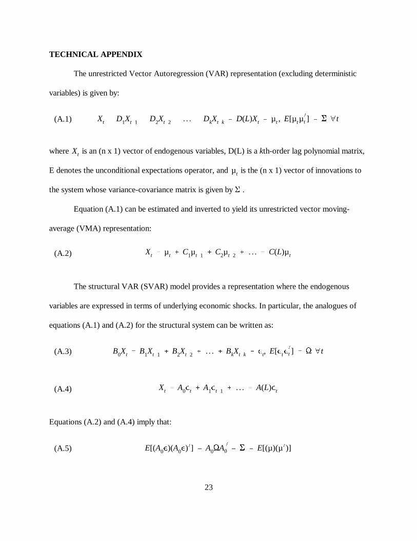
TECHNICAL APPENDIX

The unrestricted Vector Autoregression (VAR) representation (excluding deterministic

variables) is given by:

where is an (n x 1) vector of endogenous variables, D(L) is a kth-order lag polynomial matrix,

E denotes the unconditional expectations operator, and is the (n x 1) vector of innovations to

the system whose variance-covariance matrix is given by ( .

Equation (A.1) can be estimated and inverted to yield its unrestricted vector moving-

average (VMA) representation:

The structural VAR (SVAR) model provides a representation where the endogenous

variables are expressed in terms of underlying economic shocks. In particular, the analogues of

equations (A.1) and (A.2) for the structural system can be written as:

Equations (A.2) and (A.4) imply that:

A(L) C(L)A0.

A0 A0

n2

A0

A0

24

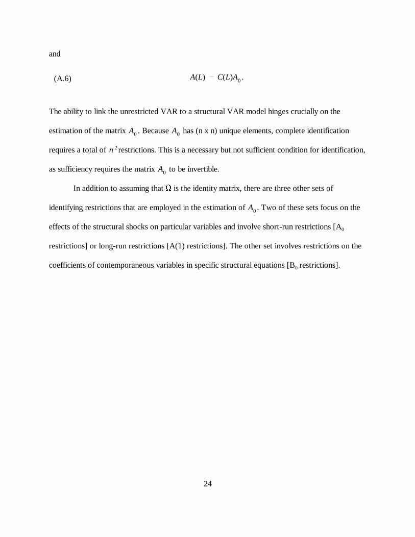
(A.6)

and

The ability to link the unrestricted VAR to a structural VAR model hinges crucially on the

estimation of the matrix . Because has (n x n) unique elements, complete identification

requires a total of restrictions. This is a necessary but not sufficient condition for identification,

as sufficiency requires the matrix to be invertible.

In addition to assuming that 6 is the identity matrix, there are three other sets of

identifying restrictions that are employed in the estimation of . Two of these sets focus on the

effects of the structural shocks on particular variables and involve short-run restrictions [A 0

restrictions] or long-run restrictions [A(1) restrictions]. The other set involves restrictions on the

coefficients of contemporaneous variables in specific structural equations [B restrictions].0

25

DATA APPENDIX

This Appendix discusses the data used in the estimation. All data are quarterly. The estimates are

conducted over the sample period 1959:Q1-1997:Q4.

Output:

The output series GDPH is measured as real gross domestic product in chain-weighted 1992

dollars.

Prices:

The price data are a quarterly average of the monthly consumer price series PCU for all urban

consumers.

Interest Rates:

The interest rate data are a quarterly average of the monthly series FTBS3 which represent the

yield on three-month Treasury bills.

Money Stock:

The data on the money stock are for M1 and are a quarterly average of the series FM1. The

measures of M1 prior to 1959 are taken from the Federal Reserve Bulletin.

26

References

Ball, Laurence M. 1994. “What determines the sacrifice ratio?” In Monetary Policy, ed. N.Gregory Mankiw. Chicago: University of Chicago Press.

Barro, Robert J. 1996. “Inflation and Growth.” Federal Reserve Bank of St. Louis. EconomicReview (May/June).

Blanchard, Olivier J. and Danny Quah. 1989. “The dynamic effects of aggregate demand andsupply disturbances.” American Economic Review 79 (September): 655-73.

Cecchetti, Stephen G. 1994. “Comment.” In Monetary Policy, ed. N. Gregory Mankiw. Chicago:University of Chicago Press.

Dickey, David A. and Wayne A. Fuller. 1981. “Likelihood ratio statistics for autoregressive timeseries with a unit root.” Econometrica 49 (November): 1057-72.

Feldstein, Martin S. 1999. ed. The Costs and Benefits of Achieving Price Stability. Chicago:University of Chicago Press, forthcoming.

Filardo, Andrew J. 1998. “New evidence on the output cost of fighting inflation.” Federal ReserveBank of Kansas City. Economic Review (Third Quarter).

Fuhrer, Jeffrey C. 1995. “The persistence of inflation and the cost of disinflation.” FederalReserve Bank of Boston. New England Economic Review (January/February).

Gali, Jordi. 1992. “How well does the IS-LM model fit postwar U.S. data?” Quarterly Journal ofEconomics 107 (May): 709-38.

Gordon, Robert J., and Stephen R. King. 1982. “The output cost of disinflation in traditional andvector autoregressive models.” Bookings Papers on Economic Activity 1:205-42.

Mankiw, N. Gregory. 1991. Macroeconomics. New York: Worth Publishers. Okun, Arthur M. 1978. “Efficient disinflationary policies.” American Economic Review 68 (May):348-52.

Pagan Adrian R. and John C. Robertson. 1998. “Structural models of the liquidity effect.” Reviewof Economics and Statistics 80 (May): 202-17. Sargent, Thomas J. 1983. “Stopping moderate inflations: The methods of Poincare and Thatcher.”In Inflation, debt, and indexation, eds. Rudiger Dornbusch and Mario H. Simonsen. Cambridge:M.I.T. Press.

27

Schelde-Andersen, Palle. 1992. “OECD country experiences with disinflation.” In Inflation,disinflation, and monetary policy, ed. Adrian Blundell-Wignell. Reserve Bank of Australia:Ambassador Press.

Shapiro, Matthew D. and Mark W. Watson. 1988. “Sources of business cycle fluctuations.” InNBER Macroeconomics Annual, eds. Olivier J. Blanchard and Stanley Fischer. Cambridge:M.I.T. Press.

Taylor, John B. 1983. “Union wage settlements during a disinflation.” American EconomicReview 73 (December): 981-93.

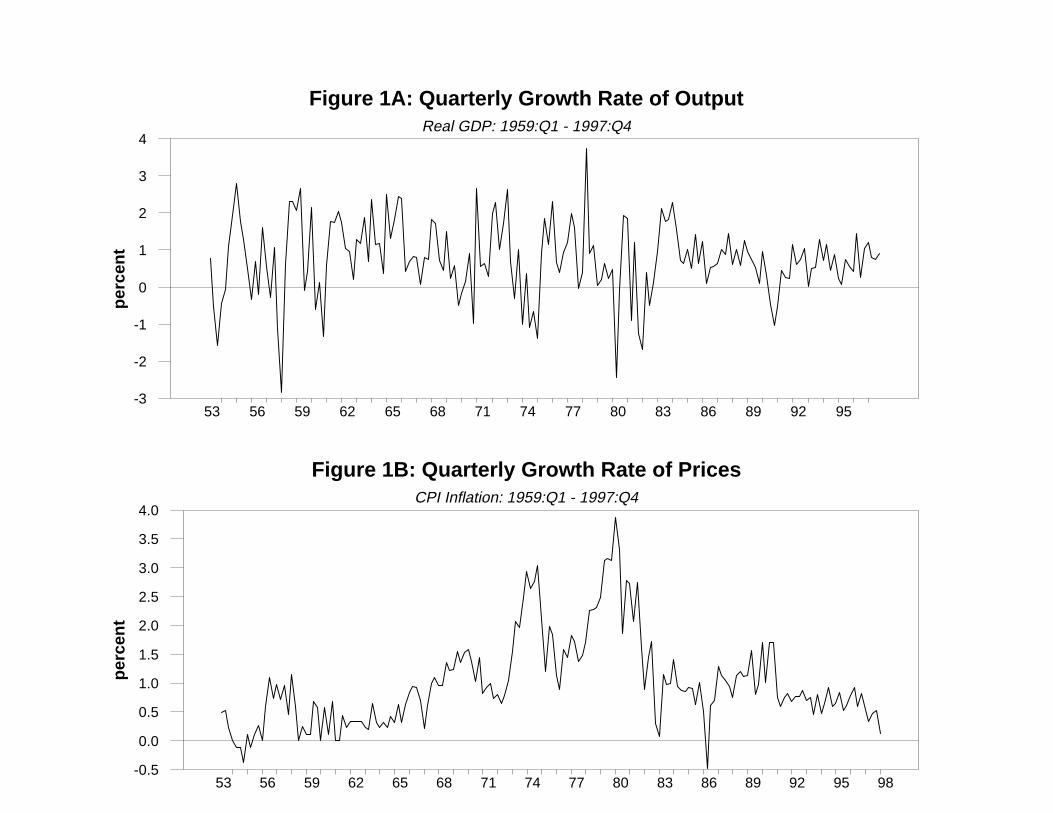
Figure 1A: Quarterly Growth Rate of OutputReal GDP: 1959:Q1 - 1997:Q4

perc

ent

53 56 59 62 65 68 71 74 77 80 83 86 89 92 95-3

-2

-1

0

1

2

3

4

Figure 1B: Quarterly Growth Rate of PricesCPI Inflation: 1959:Q1 - 1997:Q4

perc

ent

53 56 59 62 65 68 71 74 77 80 83 86 89 92 95 98-0.5

0.0

0.5

1.0

1.5

2.0

2.5

3.0

3.5

4.0

����� ���� �� �������� �� ��� ��

Calculation of the Sacrifice Ratio:Hypothetical Responses of Output and Inflationto a Contractionary Monetary Policy Shock

Figure 2

Output

Inflation

0

0

t t +

t + Time

Time

t

Area=i=0 j=0

i

a12i

a120

a220

i=0a12

i

i=0a22

i

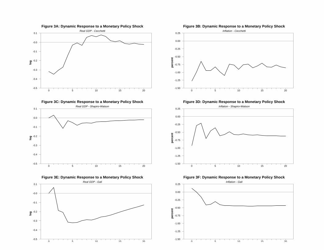
Figure 3A: Dynamic Response to a Monetary Policy ShockReal GDP - Cecchetti

log

0 5 10 15 20-0.5

-0.4

-0.3

-0.2

-0.1

-0.0

0.1

Figure 3C: Dynamic Response to a Monetary Policy ShockReal GDP - Shapiro-Watson

log

0 5 10 15 20-0.5

-0.4

-0.3

-0.2

-0.1

-0.0

0.1

Figure 3E: Dynamic Response to a Monetary Policy ShockReal GDP - Gali

log

0 5 10 15 20-0.5

-0.4

-0.3

-0.2

-0.1

-0.0

0.1

Figure 3B: Dynamic Response to a Monetary Policy ShockInflation - Cecchetti

perc

ent

0 5 10 15 20-1.50

-1.25

-1.00

-0.75

-0.50

-0.25

0.00

0.25

Figure 3D: Dynamic Response to a Monetary Policy ShockInflation - Shapiro-Watson

perc

ent

0 5 10 15 20-1.50

-1.25

-1.00

-0.75

-0.50

-0.25

0.00

0.25

Figure 3F: Dynamic Response to a Monetary Policy ShockInflation - Gali

perc

ent

0 5 10 15 20-1.50

-1.25

-1.00

-0.75

-0.50

-0.25

0.00

0.25

0

0.05

0.1

0.15

0.2

0.25

0.3

-100 -80 -60 -40 -20 0 20 40 60 80 100

Simulated Values of the Sacrifice Ratio

Fre

qu

ency

0

0.01

0.02

0.03

0.04

0.05

-100 -80 -60 -40 -20 0 20 40 60 80 100

Simulated Values of the Sacrifice Ratio

Fre

qu

ency

0

0.01

0.02

0.03

0.04

-100 -80 -60 -40 -20 0 20 40 60 80 100Simulated Values of the Sacrifice Ratio

Fre

qu

ency

Figure 4: Frequency Distribution for the Cecchetti Model2.5%-97.5% Fractile Range

Figure 5: Frequency Distribution for the Shapiro-Watson Model2.5%-97.5% Fractile Range

Figure 6: Frequency Distribution for the Gali Model2.5%-97.5% Fractile Range