
STEEL BUILDINGS IN EUROPE Single-Storey Steel Buildings Part 8
Structural Design Optimization of Steel Buildings
Using GS-USA© Frame3D
by
Yogesh Unde
A Thesis Presented in Partial Fulfillment
of the Requirements for the Degree
Master of Science
Approved November 2016 by the
Graduate Supervisory Committee:
Subramaniam Rajan, Chair
Narayanan Neithalath
Barzin Mobasher
ARIZONA STATE UNIVERSITY
December 2016

i
ABSTRACT
Tall building developments are spreading across the globe at an ever-increasing rate
(www.ctbuh.org). In 1982, the number of ‘tall buildings’ in North America was merely
1,701. This number rose to 26,053, in 2006. The global number of buildings, 200m or
more in height, has risen from 286 to 602 in the last decade alone. This dissertation
concentrates on design optimization of such, about-to-be modular, structures by
implementing AISC 2010 design requirements. Along with a discussion on and
classification of lateral load resisting systems, a few design optimization cases are also
being studied. The design optimization results of full scale three dimensional buildings
subject to multiple design criteria including stress, serviceability and dynamic response
are discussed. The tool being used for optimization is GS-USA Frame3D© (henceforth
referred to as Frame3D). Types of analyses being verified against a strong baseline of
Abaqus 6.11-1, are stress analysis, modal analysis and buckling analysis.
The provisions in AISC 2010 allows us to bypass the limit state of flexural buckling in
compression checks with a satisfactory buckling analysis. This grants us relief from the
long and tedious effective length factor computations. Besides all the AISC design
checks, an empirical equation to check beams with high shear and flexure is also being
enforced.
In this study, we present the details of a tool that can be useful in design optimization -
finite element modeling, translating AISC 2010 design code requirements into
components of the FE and design optimization models. A comparative study of designs
based on AISC 2010 and fixed allowable stresses, (regardless of the shape of cross
section) is also being carried out.

ii
ACKNOWLEDGMENTS
I consider myself very fortunate for the opportunity of working under my advisor,
Dr. Subramaniam Rajan. He did not only teach me the work, but he also taught me how
to work. I have learnt a lot from his approach towards problem solving and fundamental
thinking. This thesis experience has given me invaluable assets. I would like to express
my sincere gratitude for his guidance, supervision and encouragement throughout my
Masters program. I would also like to extend my gratitude towards Dr. Neithalath and Dr.
Mobasher for reviewing my research work.
I dedicate this work to my parents Lata and late Vinod Unde. In addition, I would
like to thank my brother Amrut Unde, whom I always look up to, and for supporting me
throughout my education.
I would also like to thank Bilal Khaled and Dr. Canio Hoffarth for all the
discussions and assistance. I would like to acknowledge all my colleagues at ASU,
friends and family for their direct and indirect support.
iii
TABLE OF CONTENTS
Page
LIST OF TABLES ............................................................................................................. vi
LIST OF FIGURES .......................................................................................................... vii
CHAPTER
1 INTRODUCTION ...................................................................................................... 1
1.1 Brief History ....................................................................................................... 1
1.2 Structural Systems and Classification ................................................................. 4
1.3 Literature Review................................................................................................ 9
1.3.1 Sizing and Shape Optimization ....................................................................... 9
1.3.2 Braced Frames .............................................................................................. 10
1.3.3 Genetic Algorithm ........................................................................................ 11
1.3.4 Method of Feasible Directions ...................................................................... 13
1.4 Research Objectives .......................................................................................... 15
2 TYPES OF ANALYSES AND STEEL STRUCTURES ......................................... 16
2.1 Finite Element Analysis – Static, Modal and Buckling .................................... 16
2.2 Buckling Analysis ............................................................................................. 17
2.3 Types of Steel Buildings and Design Codes ..................................................... 19
3 AISC 2010 DESIGN CHECKS ................................................................................ 20
3.1 Limit States and Design Requirements ............................................................. 20

iv
CHAPTER Page
3.1.1 Design of Members for Tension ................................................................... 20
3.1.2 Buckling Analysis and Compression Checks ............................................... 21
3.1.3 Modified Design Procedure .......................................................................... 23
3.1.4 Design of Members for Flexure .................................................................... 26
3.1.5 Design of Members for Shear ....................................................................... 35
3.1.6 Design of Members for Combined Effects ................................................... 37
3.2 Implemented Algorithms .................................................................................. 39
4 DESIGN OPTIMIZATION PROBLEM FORMULATION .................................... 52
4.1 Objective Function, Design Variables and Constraints in general ................... 52
4.2 Types of Design Variables ................................................................................ 53
4.3 Regression Analysis .......................................................................................... 54
4.4 Optimization Solution Techniques ................................................................... 57
4.5 Design Optimization Problem Formulation - MWD ........................................ 58
5 VALIDATION OF FEA (with ABAQUS) ............................................................... 63
5.1 Static Analysis .................................................................................................. 64
5.2 Modal Analysis ................................................................................................. 69
5.3 Redundancy of Nonlinear Geometric Analysis ................................................ 71
6 DESIGN OPTIMIZATION CASE STUDIES.......................................................... 72
6.1 Finite Element Model ....................................................................................... 72

v
CHAPTER Page
6.1.1 Building Layout ............................................................................................ 74
6.2 Nomenclature and Bracing Systems ................................................................. 77
6.3 Material Properties and Loads .......................................................................... 79
6.4 Numerical Results ............................................................................................. 82
6.4.1 General Model Information .......................................................................... 82
6.4.2 Design Properties .......................................................................................... 83
6.4.3 Weight Performance ..................................................................................... 85
7 CONCLUSIONS....................................................................................................... 89
REFERENCES ................................................................................................................. 92
APPENDIX
A DESIGN WIND LOADS ...................................................................................... 93
B AISC W SHAPES IN SELECTED TABLE ......................................................... 96
C COLUMN MOMENT OF INERTIA REQUIREMENTS .................................. 102

vi
LIST OF TABLES
Table Page
1.1 Tall Buildings in Region (Reported In Emporis) .................................................... 3
1.2 Interior Structures ................................................................................................... 7
1.3 Exterior Structures .................................................................................................. 8
4.1 C/S Properties As A Function Of Area ................................................................. 56
5.1 Nodal Displacements – LC1 ................................................................................. 65
5.2 Nodal Displacements – LC4 ................................................................................. 65
5.3 Nodal Reactions – LC1 ......................................................................................... 66
5.4 Nodal Reactions – LC4 ......................................................................................... 66
5.5 Beam Forces And Moments – LC1 ...................................................................... 67
5.6 Beam Forces And Moments – LC4 ...................................................................... 68
5.7 Lowest Frequencies .............................................................................................. 69
5.8 Highest Fundamental Periods ............................................................................... 69
5.9 Modal Eigenvalues................................................................................................ 70
6.1 General Model Information .................................................................................. 76
6.2 Material Properties ................................................................................................ 79
6.3 Dead and Live Load Intensities ............................................................................ 80
6.4 Point Mass Calculations ........................................................................................ 81
6.5 General Design Related Information .................................................................... 82
6.6 Controlling Factors and Design Properties ........................................................... 84
6.7 Weight Performance From Optimization Results ................................................. 87

vii
LIST OF FIGURES
Figure Page
1.1 Classification of Tall Buildings by Dr. Falzur Khan .............................................. 4
1.2 Interior Structures Classified by Ali and Moon ...................................................... 5
1.3 Exterior structures Classified by Ali and Moon ..................................................... 6
1.4 Braced Tube and Diagrid Structures of Various Heights, Aspect Ratios and
Optimal Angles (Kyoung Sun Moon, 2008) ......................................................... 10
1.5 Diagrid Structures with Various Diagonal Angles ............................................... 10
1.6 Flow in a Simple Optimization Algorithm ........................................................... 14
4.1 Regression Analysis : Area vs Izz .......................................................................... 55
5.1 Models for Validation of Frame3D....................................................................... 63
6.1 Space Beam Element Description ......................................................................... 72
6.2 Flowchart of the Design Process........................................................................... 73
6.3 Typical Building Plan ........................................................................................... 74
6.4 Typical Elevation of an Interior Frame ................................................................. 75
6.5 Types of Bracing Systems (Typical) for Exterior Frames .................................... 76
6.6 Highest Period vs Building Height ....................................................................... 85
6.7 Normalized Weight vs Building Height ............................................................... 88

viii
LIST OF SYMBOLS
Ae effective net area Mrx bending moment in major axis
Ag gross c/s area of member Mry bending moment in minor axis
Aw area of web Myc yield moment in compression flange
Cb lateral-torsional buckling
modification factor Nmax maximum axial force
Cw warping constant Pc available axial strength
d overall depth of the section Pn allowable axial strength
E Young’s modulus Pr required axial strength
Fcr critical stress Q net reduction factor for slender
elements
Fe elastic buckling stress Qa net reduction factor for web
ft flange thickness Qs net reduction factor for flange
fw flange width Rpc web plastification factor
Fu specified minimum tensile
strength Rpg bending strength reduction factor
Fy yield stress of steel rt effective radius of gyration for lateral-
torsional buckling
G shear modulus of steel rxx radius of gyration @ x-axis
h web height less the fillets ryy radius of gyration @ y-axis
h0 distance between flange
centroids Sx elastic section modulus @ x-axis
Ix moment of inertia @ x-axis Sxc elastic section modulus referred to
compression flange
Iy moment of inertia @ y-axis Sy elastic section modulus @ y-axis
J torsional constant U shear lag factor
K1 effective length factor at start
node Vmax maximum shear force
K2 effective length factor at end
node Vn allowable flexural strength
Kv web plate shear buckling
coefficient wh web height
Kz length factor for torsional
buckling wt web thickness
L length of the element Zx input vector
Mcx available flexural strength in
major axis Xd plastic section modulus @ x-axis
Mcy available flexural strength in
minor axis λpw
limiting slenderness for a compact
web
ix
Mmax maximum bending moment λrw limiting slenderness for a non-
compact web
Mp plastic moment capacity

1
1 INTRODUCTION
1.1 Brief History
Structural engineering dates back to 2700 B.C. when the step pyramid for Pharaoh
Djoser was built by Imhotep, the first engineer in history known by name. Pyramids were
the most common major structures built by ancient civilizations because the structural
form of a pyramid is inherently stable and can be almost infinitely scaled (as opposed to
most other structural forms, which cannot be linearly increased in size, in proportion to
increased loads).
Throughout ancient and medieval history most architectural design and
construction was carried out by artisans, such as stone masons and carpenters, rising to
the role of master builder. No theory of structures existed, and understanding of how
structures stood up was extremely limited, and based almost entirely on empirical
evidence of 'what had worked before'. Knowledge was retained by guilds and seldom
supplanted by advances. Structures were repetitive, and increases in scale were
incremental. [1]
Ironically, no record exists of the first calculations of the strength of structural
members or the behavior of structural material, but the profession of structural engineer
only really took shape with the industrial revolution and the re-invention of concrete. The
physical sciences underlying structural engineering began to be understood in the
renaissance (period in Europe, from the 14th to 17th century) and have since developed
into computer-based applications pioneered in the 1970s. [2]
Dr. Fazlur Rahman Khan was a structural engineer and architect who initiated
important structural systems for skyscrapers. ASCE gave him a title of “The father of

2
tubular designs for high-rises”. His innovation was the idea of the ‘tube’ structural system
for tall buildings, including the ‘framed tube’, ‘trussed tube’ and ‘bundled tube’
variations. Most buildings over 40-storeys, constructed since the 1960s, now use a tube
design derived from Khan's structural engineering principles. His first building to employ
the tube structure was Chestnut De-Witt apartment building in 1963. [3]
Tube structures are very stiff and have numerous significant advantages over
other framing systems. They not only make the buildings structurally stronger and more
efficient, they significantly reduce the usage of materials while simultaneously allowing
buildings to reach even greater heights. The reduction of material makes the buildings
economically much more efficient and reduces environmental issues as it results in the
least carbon emission impact on the environment. Tubular systems allow greater interior
space and further enable buildings to take on various shapes, offering unprecedented
freedom to architects. [4]
Following table shows a brief account of past developments in tall buildings.
Significance of need to optimize the use of material and carbon footprint is evident from
the numbers.

3
Region Number of
countries
1982 2006
Percent Buildings Percent Buildings
North America 4 48.9 1,701 23.9 26,053
Europe 35 21.3 742 23.7 25,809
Asia 35 20.2 702 32.2 35,016
South America 13 5.2 181 16.6 18,129
Africa 41 1.3 47 1 1,078
Total 3,373 106,085
Table 1.1 Tall buildings in region (reported in Emporis)

4
1.2 Structural Systems and Classification
In 1969, Fazlur Khan classified structural systems for tall buildings relating to
their heights with considerations for efficiency in the form of “Heights for Structural
Systems” diagrams. Later, he upgraded these diagrams by way of modifications (Khan,
1972, 1973). He developed these schemes for both steel and concrete.
Figure 1.1 Classification of tall buildings by Dr. Falzur Khan
(above: steel, below: concrete)
In 2007, Ali and Moon [5] presented a new classification – interior and exterior
structures which encompasses most representative tall building structural systems today.

5
The classification is performed for both primary structures and subsequently auxiliary
damping systems. Recognizing the importance of the premium for heights for tall
buildings, the classification of structural systems is based on lateral load-resisting
capabilities.
Figure 1.2 Interior Structures classified by Ali and Moon

6
Figure.1.3 Exterior structures classified by Ali and Moon
A detailed categorization, advantages, disadvantages, efficient height limits, etc.
is illustrated for both type of structures in tables below (Tables 1.2.1 for interior
structures and 1.2.3 for exterior structures).

7
Table 1.2 Interior structures

8
Table 1.3 Exterior structures

9
1.3 Literature Review
1.3.1 Sizing and Shape Optimization
Due to the complex nature of a modern tall building consisting of thousands of
structural members, the traditional trial-and-error design method is generally highly
iterative and very time-consuming. Chan et. al. [11] presented an automatic resizing
technique for the optimal design of tall steel building frameworks. Specifically, a
computer-based method was developed for the minimum weight design of lateral load-
resisting steel frameworks subject to multiple inter-story drift and member strength and
sizing constraints in accordance with building code and fabrication requirements. The
most economical standard steel sections to use for the structural members are
automatically selected from commercially available standard section databases. The
design optimization problem was first formulated and expressed in an explicit form and
was then solved by a rigorously derived optimality criteria algorithm. A full-scale 50-
story three-dimensional asymmetrical building framework example was presented to
illustrate the effectiveness, efficiency, and practicality of the automatic resizing
technique. The efficiency of the iterative resizing technique presented, was influenced by
the number of constraints and is only weakly dependent on the number of variables. The
method provides an effective strategy for the optimal design of tall buildings involving
many sizing variables and comparatively fewer drift constraints. An interesting finding is
that the optimal design of an asymmetric building framework corresponds to a state in
which there is little or almost no building torsion.

10
1.3.2 Braced Frames
Moon [10] discussed stiffness-based design methodologies for tall building
structures with an emphasis on systems with diagonals such as braced tubes and diagrid
structures. Guidelines for determination of bending and shear deformations for optimal
design, which uses the least amount of structural material to meet the stiffness
requirements were presented. The impact of different geometric configurations of the
structural members on the material saving economic design is also discussed and
recommendations for optimal geometries are made.
Figure 1.5 Diagrid structures with various diagonal angles
As seen in figures 1.3.2 and 1.3.3, structures of various heights and varying
diagrid angles were studied. It was observed that braced framed tube systems performed
Figure 1.4 Braced tube and Diagrid structures of various heights, aspect ratios and
optimal angles (Kyoung Sun Moon, 2008)

11
best at a diagonal angle nearing 47°. It was also observed with diagrid systems that 63° is
near the optimal angle for up to 50 story structures and 69° for structures for and above
60 storeys.
1.3.3 Genetic Algorithm
GA is basically a Direct Search technique, which does not require derivatives.
Hence GA has the advantage of being able not only to solve problems where the
derivatives are discontinuous but also to find the global minimum. This advantage is
offset by an increase in computational requirement – usually the function values are
required at a very large number of locations in the design space. The advantage of using
GA is that it can handle various types of design variables, including DDV, CDV and
Boolean variables. As a result, around 95 percent of structural design optimization work
is carried out by implementing GA.
GA is a search strategy based on the rules of natural genetic evolution. Even
before the traits of genetic systems were used in solving optimization problems,
biologists have used computers to perform simulations of genetic system by the early
1950s. The application of GAs for adaptive systems was first proposed by John Holland
(University of Michigan) in 1962.
Because of their discrete nature, GAs lend themselves well to the process of
automating the design of skeletal structures. GAs do not require gradient or derivative
information. For this reason alone, they have been applied y researchers to solve discrete,
non-differentiable, combinatory and global optimization engineering problems, such as
transient optimization of gas pipeline, topology design of general elastic mechanical
systems, time scheduling, circuit layout design, composite panel design, pipe network

12
optimization and so on and so forth. GAs are recognized as different from traditional
gradient based optimization techniques in the following four major ways [Goldberg,
1989]:
1. GAs work with coding of the design variables and parameters in the problem,
rather than the actual parameters themselves.
2. GAs make use of population type search. Many different design points are
evaluated during each iteration instead of sequentially moving from one point to
the next
3. GAs need only a fitness or objective function value. No derivatives or gradients
are necessary.
4. GAs use probabilistic transition rules to find new design points for exploration
rather than using deterministic rules based on gradient information to find these
new points.

13
1.3.4 Method of Feasible Directions
The numerical Gradient-based techniques are particularly useful when designing
with continuous design variables and continuous and differentiable objective and
constraint values. In particular, the Method of Feasible Directions (MFD) [Rajan et al.,
2006] is used in this study. Typical problems with about 25-50 design variables can be
solved in about 10-15 iterations involving less than a hundred function evaluations and
about 10-15 gradient evaluations. The active set strategy is used in order to make the
storage space and computations efficient.
Although there are many variations of optimization techniques in existence, the
basic structure is that shown in figure 1.3.3.1. [6]

14
Figure 1.6 Flow in a simple optimization algorithm

15
1.4 Research Objectives
Most of the structural optimization research is carried out considering the strength
based, deflection and drift constraints as design requirements. This work concentrates on
structural design optimization of interior and exterior planar frames of ten, twenty, forty
and sixty storey buildings. Since it is unconventional to provide bracings in internal
frames, the interior frames are necessarily assumed to be ‘rigid’ type structures. For
exterior frames, six different types of bracing systems are being designed and optimized
for all four buildings. All models are being optimized with AISC 2010 constraints as well
as strength based constraints (as separate finite element models) for comparison purposes.
Also, lateral deflection, inter-story drift and Euler buckling constraints are being enforced
in all models.
An algorithm has been developed from AISC 2010 specifications manual for I-
sections and implemented in GS-USA Frame3D program. The structural analysis and
design optimization of the building models is accomplished by using the Frame3D
program.

16
2 TYPES OF ANALYSES AND STEEL STRUCTURES
2.1 Finite Element Analysis – Static, Modal and Buckling
The Finite Element Method (FEM) has evolved over a long time. The basic
building blocks and ideas originated in the 1940s. With the advancement of technology
and computers in 1950s, the ideas were converted into matrix form, making it possible
for a practical implementation. [6]
The finite element method is a computer-aided mathematical technique for
obtaining approximate numerical solutions to the abstract equations of calculus that
predict the response of physical systems subjected to external influences. [7]
Various types of finite element analyses can be applied to pose a single problem,
usually a function evaluation, and sometimes to compute constraints. In civil engineering
structural analysis, three sets of algebraic equations and/or Eigenvalue problems are
solved as follows.
,e d d d lc d lc K D = F (2.1.1)
,e d d d d d d d d d d K Φ = Λ M Φ (2.1.2)
, ,B
e d d d lc g d d d lc K D K D (2.1.3)
where ,e d dK , d dM and ,g d dK are the elastic structure stiffness matrix, mass
matrix and geometric stiffness matrix respectively. Also, ‘d’ is the effective number of
degrees-of-freedom in the finite element model, ‘lc’ is the number of load cases, ‘ B ’ is
the buckling load factor for the lowest mode. Equations (2.1.2) and (2.1.3) are typically
solved in smaller subspaces as ,ˆ ˆ
e q q q q q q q q q q K Φ = Λ M Φ and
17
, ,ˆ ˆB
e q q g q qq lc q lc K D K D , since only the lowest few ‘q’ Eigen-pairs are of
interest. Detailed explanation on buckling analysis follows.
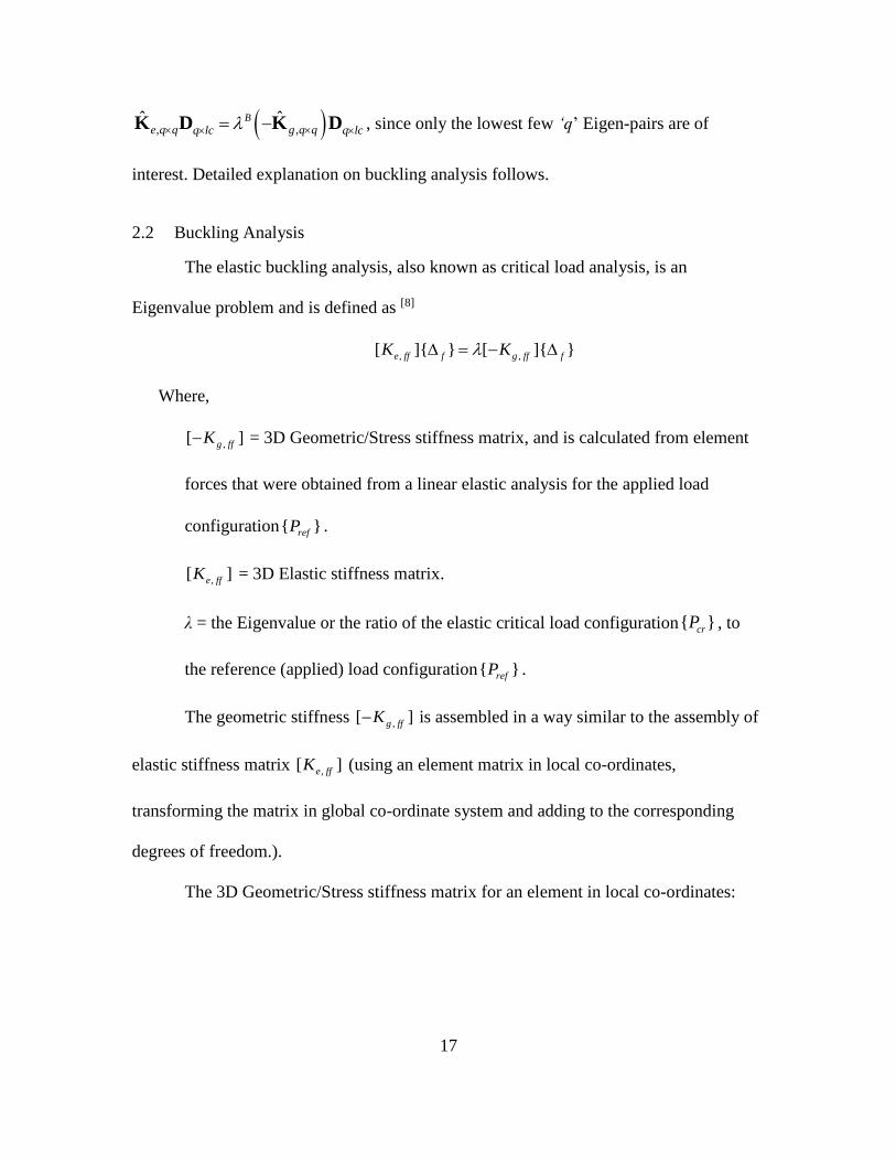
2.2 Buckling Analysis
The elastic buckling analysis, also known as critical load analysis, is an
Eigenvalue problem and is defined as [8]
, ,[ ]{ } [ ]{ }e ff f g ff fK K
Where,
,[ ]g ffK = 3D Geometric/Stress stiffness matrix, and is calculated from element
forces that were obtained from a linear elastic analysis for the applied load
configuration{ }refP .
,[ ]e ffK = 3D Elastic stiffness matrix.
λ = the Eigenvalue or the ratio of the elastic critical load configuration{ }crP , to
the reference (applied) load configuration{ }refP .
The geometric stiffness ,[ ]g ffK is assembled in a way similar to the assembly of
elastic stiffness matrix ,[ ]e ffK (using an element matrix in local co-ordinates,
transforming the matrix in global co-ordinate system and adding to the corresponding
degrees of freedom.).
The 3D Geometric/Stress stiffness matrix for an element in local co-ordinates:

18
2 2
2 2
2
2
2
1 0 0 0 0 0 1 0 0 0 0 0
1.2 0 0 0 0 1.2 0 0 010 10
1.2 0 0 0 0 1.2 0 010 10
0 0 0 0 0 0 0
20 0 0 0 0
15 10 30
20 0 0 0
15 10 30[ ]
1 0 0 0 0 0
1.2 0 0 010
1.2 0 010
. 0 0
20
15
2
15
xg
L L
L L
J J
A A
L L L
L L L
FK
L
L
L
JSYM
A
L
L
Where,
Fx2 = axial force in the element (negative if compressive and positive if
tensile) as a result of linear elastic analysis for the applied loads.
L = Length of the element.
J = Torsional constant.
Jacobi method has been implemented to solve the EVP and obtain the first few
Eigenvalues. Therefore, it can be said that, if the first and lowest Eigenvalue is less than

19
1, i.e. { }
1{ }
cr
ref
P
P , the structure has undergone buckling for the applied load configuration
and vice-versa.
2.3 Types of Steel Buildings and Design Codes
This dissertation concentrates on design optimization of planar frames of tall steel
buildings, up to sixty storeys. Since it is not a general practice to provide bracing
elements (topology optimization) in interior frames of an office building, two different
sets of models are being created, namely, interior and exterior frames. Interior frames are
being designed for sizing and shape optimization, whereas exterior frames are being
optimized in three areas viz., sizing, shape and topology.
Although, many literatures have established optimum framing systems for
exterior structures (figure 1.2.3) as a function of the height, the width is seldom a
parameter for optimum designs. For this reason, exterior frames will be optimized
topologically using (i) belt trusses, (ii) diagrid systems. and (iii) exo-skeleton types of
bracing systems. Regardless of what has been previously established, optimum topology
systems will be defined for a particular width and varying heights.
All the steel structures are being designed by implementing AISC 2010
specifications. To carry out a comparative study, all frames designed in accordance with
AISC 2010 specifications, are also being designed for strength based constraints
(Equation B3-1, AISC 2005). This will also give us confidence in the newly developed
technique.

20
3 AISC 2010 DESIGN CHECKS
3.1 Limit States and Design Requirements
3.1.1 Design of members for tension
1. Slenderness limitations.
The slenderness ratio L/r preferably should not exceed 300. Where r is minimum
of rxx and ryy.
2. Tensile strength.
The allowable tensile strength, Pn/Ωt, of tension members shall be the lower value
obtained according to the limit states of tensile yielding in the gross section and
tensile rupture in the net section.
1. For tensile yielding in the gross section
Pn = Fy Ag (D2-1 AISC 2010)
Ωt = 1.67 and Ag = gross area of the section
2. For tensile rupture in the net section
Pn = Fu Ae
Ωt = 2.0 and Ae = effective net area = 0.8 Ag U (D2-2 AISC 2010)
Note: Assuming 20% of area for bolt holes.
U = shear lag factor (maximum of U1 and U2)
U1 = 2 fw ft / Ag, (D-3 AISC 2010)
If fw ≥ 2/3 d: U2 = 0.9, else U2 = 0.85 (Table D3.1 Case 7)

21
3.1.2 Buckling Analysis and Compression Checks
According to Chapter E in AISC 2010 construction manual, the nominal
compressive strength, Pn, shall be the lowest value obtained based on the applicable limit
states of flexural buckling, torsional buckling and flexural-torsional buckling.
In the case of flexural buckling, the elastic buckling stress is determined
according to equation E3-4, as specified in Appendix 7, section 7.2.3(b), or through an
elastic buckling analysis, as applicable.
2
2e
EF
KL
r
(E3-4 AISC 2010)
This conventional method of arriving at the elastic buckling stress, known as
effective length method, needs the determination of accurate ‘K’ factors by tedious hand
procedures and approximate ‘charts’ provided in the manual. Furthermore, these charts
are based on assumptions of idealized conditions, which seldom exist in real structures.
These assumptions are as follows:
1. Behavior is purely elastic.
2. All members have constant cross section.
3. All joints are rigid.
4. For columns in frames with sidesway inhibited, rotations at opposite ends of
the restraining beams are equal in magnitude and opposite in direction,
producing single curvature bending.
5. For columns in frames with sidesway uninhibited, rotations at opposite ends
of the restraining beams are equal in magnitude and direction, producing
reverse curvature bending.

22
6. The stiffness parameter 𝐿√𝑃/𝐸𝐼 of all columns is equal.
7. Joint restraint is distributed to the column above and below the joint in
proportion to EI/L for the two columns.
8. All columns buckle simultaneously.
9. No significant axial compression force exists in the girders.
Keeping in mind these assumptions, adjustments are often required for
(i) Columns with different end conditions.
(ii) Girders with different end conditions.
(iii) Girders with significant axial loads.
(iv) Column inelasticity.
AISC 2010 does not account for the rotational stiffness provided by non-
orthogonal members in a structure. Even after implementing all the above stated
conditions in an analysis software, it is very difficult to extract the K values from the
‘alignment charts’ provided in the manual (Fig. C-A-7.1 and Fig. C-A-7.2). In order to
avoid these complications and tedious procedures, it is only wise to get the buckling
strength of the structure via elastic buckling analysis.
In other words, we can design the structure in such a manner that the lowest
Eigenvalue is greater than 1. This implies that the applied loads are not enough for any
element in the structure to buckle.
Hence, if the lowest Eigenvalue is greater than 1, it is no longer necessary to
check for the limit state of flexural buckling (elastic and/or inelastic buckling) in
compression checks. AISC Commentary section 1.3 - 16.1–473 defines the required axial

23
compressive strengths of all members whose flexural stiffness are considered to
contribute to lateral stability of the structure, should satisfy the limitation:
0.75r yP P
Where,
Pr = required axial compressive strength under LRFD or ASD load
combinations, kips.
y y gP F A , the axial yield strength, kips.
3.1.3 Modified design procedure
The nominal compressive strength, Pn, shall be the lowest value obtained based on
the applicable limit states of flexural buckling, torsional buckling, and flexural-torsional
buckling.
The allowable compressive strength = Pn / Ωc
Where,
Ωc = 1.67 (Allowable strength design) and
Pn is the nominal compressive strength.
a. Limit state of flexural buckling – for members without slender elements
n cr gP F A (E3-1 AISC 2010)
0.75cr yF F
b. Limit state of torsional and flexural – torsional buckling – without slender
elements
The critical stress Fcr shall be determined as follows:

24
i. When 2.25y
e
F
F : 0.658
y
e
F
F
cr yF F
(E7-2 AISC 2010)
ii. When 2.25y
e
F
F : 0.877cr eF F (E7-3 AISC 2010)
Torsional or flexural – torsional buckling stress, Fe, is determined as
2
2
1we
x yz
ECF GJ
I IK L
(E4-4 AISC 2010)
G = Shear modulus of steel
J = Torsional constant
Kz = Effective length factor for torsional buckling
Note: Assuming Kz = 1.0 (AISC pg. 16.1-296)
Cw = Warping constant:
2
0
4
y
w
I hC
h0 = distance between flange centroids
Pn shall be calculated as per section ‘a’ above.
c. Members with slender elements
The critical stress Fcr shall be minimum of:
i. 0.75cr yF QF
ii. When 2.25y
e
QF
F : 0.658
y
e
F
F
cr yF Q F
(E7-2 AISC 2010)
iii. When 2.25y
e
QF
F : 0.877cr eF F (E7-3 AISC 2010)
Where,

25
Fe = elastic buckling stress calculated from E4-4
Q = net reduction factor accounting for all slender compression elements
= QsQa
For sections composed of only slender flange elements, Qa = 1.
For sections composed of only slender web, Qs = 1.
Net reduction factor calculations
1. Slender flange elements, Qs
a. When 0.562
w
t y
f E
f F : Qs = 1.0
b. When 0.56 1.032
w
y t y
fE E
F f F : 1.415 0.74
2
yws
t
FfQ
f E
c. When 1.032
w
t y
f E
f F :
2
0.69
2
s
wy
t
EQ
fF
f
2. Slender web elements, Qa
ea
g
AQ
A
where,
Ae = summation of effective areas of the cross section based on the
reduced effective width be
be is determined as follows
when 1.492
w
t y
f E
f F ,
0.341.92 1
/ 2 2
we t
cr w t cr
fE Eb f
F f f F
with Fcr is calculated based on Q = 1.0

26
3.1.4 Design of members for flexure
The allowable flexural strength = Mn / Ωb
Where Ωb = 1.67 (Allowable strength design) and Mn is the nominal flexural
strength.
Cb, The lateral-torsional buckling modification factor for non-uniform moment
diagrams when both ends of segments are braced is given by:
max
max
12.5
2.5 3 4 3b
A B C
MC
M M M M
(F1-1 AISC 2010)
Where,
Mmax = absolute value of maximum moment in the unbraced segment
MA = absolute value of moment at quarter point of the unbraced segment
MB = absolute value of moment at center-line of the unbraced segment
MC = absolute value of moment at three-quarter point of the unbraced segment
For cantilevers or overhangs, where the free end is unbraced, Cb = 1.0
For equal end moments of opposite signs, Cb = 1.0
1. Major axis bending
1. Compact I-shaped members
Mn shall be lower value obtained according to the limit states of yielding
(plastic moment) and lateral-torsional buckling.
1. Limit state of yielding
n p y xM M F Z (F2-1 AISC 2010)
Where,
27
Fy = specified minimum yield stress of the type of steel being used
Zx = plastic section modulus about the x-axis.
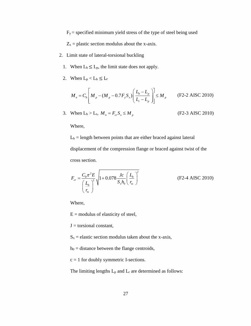
2. Limit state of lateral-torsional buckling
1. When Lb ≤ Lp, the limit state does not apply.
2. When Lp < Lb ≤ Lr
( 0.7 )b p
n b p p y x p
r p
L LM C M M F S M
L L
(F2-2 AISC 2010)
3. When Lb > Lr, n cr x pM F S M (F2-3 AISC 2010)
Where,
Lb = length between points that are either braced against lateral
displacement of the compression flange or braced against twist of the
cross section.
22
2
0
1 0.078b bcr
x tsb
ts
C E LJcF
S h rL
r
(F2-4 AISC 2010)
Where,
E = modulus of elasticity of steel,
J = torsional constant,
Sx = elastic section modulus taken about the x-axis,
h0 = distance between the flange centroids,
c = 1 for doubly symmetric I-sections.
The limiting lengths Lp and Lr are determined as follows:

28
1.76p y
y
EL r
F (F2-5 AISC 2010)
2 2
0 0
0.71.95 6.76
0.7
y
r ts
y x x
FE Jc JcL r
F S h S h E
(F2-6 AISC 2010)
Where, 2 y w
ts
x
I Cr
S (F2-7 AISC 2010)
2. I-shaped members with compact webs and non-compact or slender flanges
Mn shall be lower value obtained according to the limit states of lateral-
torsional buckling and compression flange local buckling.
1. For limit state of lateral-torsional buckling, same provisions as compact I
sections shall apply.
2. Limit state of compression flange local buckling
1. For sections with non-compact flanges
( 0.7 )pf
n p p y x p
rf pf
M M M F S M
2. For sections with slender flanges
2
0.9 c xn
EK SM
where,
λ = fw / 2ft,
0.38pf
y
E
F (limiting slenderness for compact flange)
rf
y
E
F (limiting slenderness for non-compact flange)

29
40.35 0.76
/c
t
Kh w
where,
h = web height less the fillet radii
3. I-shaped members with non-compact webs
Mn shall be lowest value obtained according to the limit states of
compression flange yielding, lateral-torsional buckling and compression
flange local buckling.
1. Compression flange yielding
n pc yc pc y xcM R M R F S
where,
Myc = yield moment in compression flange
2. Lateral-torsional buckling
1. When Lb ≤ Lp, the limit state of lateral-torsional buckling does not
apply.
2. When Lp < Lb ≤ Lr,
0.7b p
n b pc yc pc yc y xc pc yc
r p
L LM C R M R M F S R M
L L
3. When Lb > Lr, n cr xc pc ycM F S R M
where, yc y xcM F S
22
2
0
1 0.078b bcr
xc tb
t
C E LJF
S h rL
r

30
For / 0.23yc yI I : J = 0
Where,
Iyc = moment of inertia of the compression flange about the y-axis
The limiting laterally unbraced length for the limit state of yielding is
given by: 1.1p t
y
EL r
F
The limiting unbraced length for the limit state of inelastic lateral-
torsional buckling is given by:
2 2
0 0
0.71.95 6.76
0.7
y
r t
y xc xc
FE J JL r
F S h S h E
The web plastification factor, Rpc is given by
1. When Iyc / Iy > 0.23
i. When pw : Rpc = Mp / Myc
ii. When pw : 1p p pw p
pc
yc yc rw pw yc
M M MR
M M M
2. When Iyc / Iy ≤ 0.23: Rpc = 1.0
Where,
Mp = Fy Zx ≤ 1.6 Fy Sxc
Sxc = elastic section modulus referred to compression flange (AISC
2010 pg. 16.1-311)
c
t
h
W

31
λpw = the limiting slenderness for a compact web
λrw = the limiting slenderness for a non-compact web
hc = twice the distance from the centroid to the inside face of the
compression flange less the fillet or corner radius.
The effective radius of gyration for lateral-torsional buckling, rt, is
given by2
0
0
126
wt
w h
fr
h a W
d h d
, where c tw
w t
h Wa
f f
3. Compression flange local buckling
1. For sections with compact flanges, the limit state of local buckling does
not apply.
2. Sections with non-compact flanges,
0.7pf
n pc yc pc yc y xc
rf pf
M R M R M F S
3. For sections with slender flanges,
2
0.9 c xcn
Ek SM
where all parameters are as defined earlier.
4. I-shaped members with slender webs
Mn shall be lowest value obtained according to the limit states of
compression flange yielding, lateral-torsional buckling and compression
flange local buckling.

32
1. Compression flange yielding
n pg y xcM R F S
2. Lateral torsional buckling
Mn = Rpg Fcr Sxc
1. When Lb ≤ Lp, the limit state of lateral-torsional buckling does not
apply.
2. When Lp < Lb ≤ Lr, (0.3 )b p
cr b y y y
r p
L LF C F F F
L L
3. When Lb > Lr, 2
2
bcr y
b
t
C EF F
L
r
Where,
1.1p t
y
EL r
F ,
0.7r t
y
EL r
F ,
Rpg = bending strength reduction factor:
1 5.7 1.01200 300
w cpg
w t y
a h ER
a W F
,
10c tw
w t
h Wa
f f ,
2
0
0
126
wt
w h
fr
h a W
d h d

33
3. Compression flange local buckling
Mn = Rpg Fcr Sxc
1. For sections with compact flanges, the limit state of compression flange
local buckling does not apply.
2. For sections with non-compact flanges
(0.3 )pf
cr y y
rf pf
F F F
3. For sections with slender flanges
2
0.9 ccr
EkF
Where,
40.35 0.76
/c
t
Kh w
,
2
w
t
f
f

34
2. Minor axis bending
Mn shall be lower value obtained according to the limit states of yielding
(plastic moment) and flange local buckling.
1. Yielding
= 1.6 n p y y y yM M F Z F S
2. Flange local buckling
1. For sections with compact flanges, the limit state of flange local buckling
does not apply.
2. For sections with non-compact flanges
( 0.7 )pf
n p p y y
rf pf
M M M F S
3. For sections with slender flanges
n cr yM F S
Where,
2
0.69cr
EF
λ = fw / 2ft
Sy = elastic section modulus taken about the y-axis.

35
3.1.5 Design of members for shear
The allowable flexural strength = Vn / Ωv
Where Ωv = 1.67 (Allowable strength design)
and Vn is the nominal shear strength.
1. Shear strength – major axis
The nominal shear strength Vn, of unstiffened or stiffened webs according to the
limit state of shear yielding and shear buckling is
0.6n y w vV F A C (G2-1 AISC 2010)
Where,
Aw = area of web, overall depth times the web thickness, d wt,
h = the clear distance between flanges less the fillet or corner radii,
wt = thickness of web.
For Cv,
a. If 2.24t y
h E
w F , Ωv = 1.50 and Cv = 1.0.
b. Else,
i. When 1.10 v
t y
h EK
w F , Cv = 1.0
ii. When 1.10 1.37v v
y t y
E h EK K
F w F ,
1.10 v
y
v
t
EK
FC
h
w
(G2-4 AISC 2010)

36
iii. When 1.37 v
t y
h EK
w F ,
2
1.51 vv
y
t
K EC
hF
w
(G2-5 AISC 2010)
The web plate shear buckling coefficient, Kv, for webs without transverse
stiffeners and with 260t
h
w , Kv = 5.
2. Shear strength – minor axis (G7 AISC 2010)
For doubly symmetric shapes loaded in the weak axis without torsion, the
nominal shear strength, Vn, for each shear resisting element shall be determined
using equation G2-1 and section G2-1(b) with 2 , / / , 1.2w f f w f vA b t h t b t k ,
and b = half of the full-flange width, bf in. (mm).
Note: For all ASTM A6 W shapes, when 50yF ksi (345 MPa), Cv = 1.0

37
3.1.6 Design of members for combined effects
1. Members subjected to flexure and compression.
The interaction of flexure and compression shall be limited by:
a. When 0.2r
c
P
P ,
81.0
9
ryrxr
c cx cy
MMP
P M M
(H1-1a AISC 2010)
b. When 0.2r
c
P
P ,
81.0
2 9
ryrxr
c cx cy
MMP
P M M
(H1-1b AISC 2010)
Where,
Pr = Required axial strength using ASD load combinations,
Pc = Available axial strength = Pn / Ωc,
Mr = Required flexural strength,
Mc = Available flexural strength = Mn / Ωb,
x: Subscript relating symbol to strong axis bending and shear,
y: Subscript relating symbol to weak axis bending and shear.
2. Members subjected to flexure and tension
The interaction of tension and flexure, constrained to bend about a geometric
axis (x and/or y) shall be limited by equations H1-1a and H1-1b.
Where,
Pc = Available axial strength, = Pn / Ωt
Allowable tensile strength Pn / Ωt shall be the lower value obtained according
to the limit states of tensile yielding in the gross section and tensile rupture in
the net section.

38
1. For tensile yielding in the gross section
Pn = Fy Ag and Ωt = 1.67
2. For tensile rupture in the net section
Pn = Fu Ae and Ωt = 2.00
Where,
Ae = effective net area,
Ag = gross area of the member,
Fy = specified minimum yield stress,
Fu = specified minimum tensile strength.
Cb in equation F1-1 may be multiplied by 1 r
ey
P
P
for axial tension that acts
concurrently with flexure. Where
2
2
y
ey
b
EIP
L
and α = 1.6
3. Members subjected to high flexure and high shear
When a beam element is subjected to relatively large shear and bending moment
at the same location, the beam cannot provide its full capacity either in shear or in
moment. As a result, an empirical interaction equation is used to check the
adequacy of the beam. Vc = Available shear strength = Vn / Ω
If 0.6 c u cV V V , and if 0.75 c u cM M M with Ω = 1.67, beams must satisfy
the following interaction equations. [9]
1. 0.625 1.375ux ux
cx cx
M V
M V
2. 0.625 1.375uy uy
cy cy
M V
M V

39
3.2 Implemented algorithms
3.2.1a Design checks for tensile force
1. Get the length, rxx and ryy of the member;
r = minimum of rxx and ryy
2. If L/ r < 300: check (1) = OK,
else: check (1) = slender element.
3. Get the axial force Pa, Fy and Ag of the member.
4. Tensile strength in yielding: 1 /1.67n y gP F A
5. Get the element properties vector dX
6. Total depth of section, d = wh + 2 ft
7. Shear lag factor:
U1 = 2 fw ft / Ag
If fw ≥ 2/3 d: U2 = 0.85,
else U2 = 0.9
8. U = maximum of U1 and U2
9. Effective net area Ae = 0.8Ag U (Assuming 20% bolt holes)
10. Tensile strength in rupture: 2 0.5n u eP F A
11. Pn = minimum of Pn1 and Pn2
12. Return Pa / Pn:
40
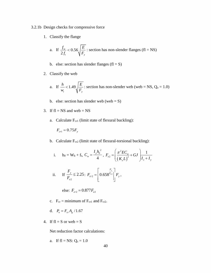
3.2.1b Design checks for compressive force
1. Classify the flange
a. If 0.562
w
t y
f E
f F : section has non-slender flanges (fl = NS)
b. else: section has slender flanges (fl = S)
2. Classify the web
a. If 1.49t y
h E
w F : section has non-slender web (web = NS, Qa = 1.0)
b. else: section has slender web (web = S)
3. If fl = NS and web = NS
a. Calculate Fcr1 (limit state of flexural buckling):
1 0.75cr yF F
b. Calculate Fcr2 (limit state of flexural-torsional buckling):
i. h0 = Wh + ft,
2
0
4
y
w
I hC ,
2
2 2
1we
x yz
ECF GJ
I IK L
ii. If 2
2.25y
e
F
F : 2
2 0.658
y
e
F
F
cr yF F
,
else: 2 20.877cr eF F
c. Fcr = minimum of Fcr1 and Fcr2.
d. /1.67n cr gP F A
4. If fl = S or web = S
Net reduction factor calculations:
a. If fl = NS: Qs = 1.0

41
b. If 0.56 1.032
w
y t y
fE E
F f F : 1.415 0.74
2
yws
t
FfQ
f E
c. else if 1.032
w
t y
f E
f F :
2
0.69
2
s
wy
t
EQ
fF
f
d. If 1.492
w
t y
f E
f F :
i. 1 0.75cr yF F
ii. 0 h th W f ,
2
0
4
y
w
I hC ,
2
2 2
1we
x yz
ECF GJ
I IK L
iii. If 2
2.25y
e
F
F : 2
2 0.658
y
e
F
F
cr yF F
,
else: 2 20.877cr eF F
e. Fcr = minimum of Fcr1 and Fcr2.
f. 0.34
1.92 1/ 2
e t
cr w t cr
E Eb f b
F f f F
, ( ) (4 )e h t e tA W W b f
g. ea
g
AQ
A , s aQ Q Q
h. check:
i. 1 0.75cr yF QF
ii. 0 h th W f ,
2
0
4
y
w
I hC ,
2
2 2
1we
x yz
ECF GJ
I IK L

42
iii. If2
2.25y
e
F
F : 2
2 0.658
y
e
F
F
cr yF Q F
,
else: 2 20.877cr eF F
i. Fcr = minimum of Fcr1 and Fcr2.
j. /1.67n cr gP F A
k. Pn = minimum of Pn(3), Pn(4)
5. Return Pa / Pn:

43
3.2.2a Design checks for shear force (major axis)
1. If 2.24t y
h E
w F : Ωv = 1.50 and Cv = 1.0,
else: Ωv = 1.67
2. Kv = 5.0
3. If 1.10 v
t y
h EK
w F : Cv = 1.0
4. Else if 1.10 1.37v v
y t y
E h EK K
F w F :
1.10 v
y
v
t
EK
FC
h
w
5. Else if 1.37 v
t y
h EK
w F :
2
1.51 vv
y
t
K EC
hF
w
6. Vn = 0.6 Fy Aw Cv / Ωv
7. Return (Va / Vn)

44
3.2.2b Design checks for shear force (minor axis)
1. If 2.242
w
t y
f E
f F : Ωv = 1.50 and Cv = 1.0,
else: Ωv = 1.67
2. Kv = 1.2, 2 ww tA f f
3. If 1.102
wv
t y
f EK
f F : Cv = 1.0
4. Else if 1.10 1.372
wv v
y t y
fE EK K
F f F :
1.10
2
v
y
vw
t
EK
FC
f
f
5. Else if 1.372
wv
t y
f EK
f F :
2
1.51
2
vv
wy
t
K EC
fF
f
6. Vn = 0.6 Fy Aw Cv / Ωv
7. Return (Va / Vn)

45
3.2.3a Design checks for flexure (major axis)
1. Classify the flange
a. If 0.382
w
t y
f E
f F : section has compact flanges (fl = C)
b. If 0.382
w
y t y
fE E
F f F : section has non-compact flanges (fl = NC)
c. If 2
w
t y
f E
f F : section has slender flanges (fl = S)
2. Classify the web
a. If 3.76t y
h E
w F : section has compact web (web = C)
b. If 3.76 5.7y t y
E h E
F w F : section has non-compact web (web = NC)
c. If 5.7t y
h E
w F : section has slender web (web = S)
3. If check is being carried out for flexure and tension:
2
max
2
max
1.6 12.51
2.5 3 4 3
r bb
y A B C
P L MC
EI M M M M
else: max
max
12.5
2.5 3 4 3b
A B C
MC
M M M M
4. If section is compact (web = C and fl = C):
a. Yielding: Mn1 = Mp = Fy Zx
b. L-T buckling: 1.76p y
y
EL r
F , Lb = L, h0 = Wh + ft

46
i. If Lb < Lp: Mn2 = Mn1
ii. 2 y w
ts
x
I Cr
S ,
2 2
0 0
0.71.95 6.76
0.7
y
r ts
y x x
FE J JL r
F S h S h E
iii. If Lp < Lb ≤ Lr: 2 ( 0.7 )b p
n b p p y x p
r p
L LM C M M F S M
L L
iv. If Lb > Lr:
22
2
0
1 0.078b bcr
x tsb
ts
C E LJF
S h rL
r
,
Mn2 = Fcr Sx
c. Mn = minimum of Mn1 and Mn2
5. If fl = NC or fl = S and web = C
a. For lateral torsional buckling, obtain Mn1 from 4.b
b. Compression flange local buckling:
i. λ = fw / 2ft, 0.38pf
y
E
F ,
rf
y
E
F
ii. If fl = NC: 2 ( 0.7 )
pf
n p p y x p
rf pf
M M M F S M
iii. If fl = S: 4
0.35 0.76/
c
t
Kh w
, 2 2
0.9 c xn
EK SM
c. Mn = minimum of Mn1 and Mn2
6. If web = NC
a. Iyc = Moment of inertia of the compression flange @ y-axis = ft fw3 / 12
b. hc = h, Sxc = Sxt = Ix / (Wh/2 + ft)

47
c. Mp = Fy Zx ≤ 1.6 Fy Sxc, Myc = Fy Sxc, 3.76pw
y
E
F , c
t
h
W
d. If Iyc / Iy > 0.23
i. If pw : Rpc = Mp / Myc
ii. If pw : 5.7rw
y
E
F , 1
p p pw p
pc
yc yc rw pw yc
M M MR
M M M
e. If Iyc / Iy ≤ 0.23: Rpc = 1, J = 0
f. Compression flange yielding: Mn1 = Rpc Myc
g. L-T buckling: Lb = L, c tw
w t
h Wa
f f , h0 = Wh + ft ,
2
0
0
126
wt
w h
fr
h a W
d h d
,
1.1p t
y
EL r
F ,
2 2
0 0
0.71.95 6.76
0.7
y
r t
y xc xc
FE J JL r
F S h S h E
i. If Lb ≤ Lp: Mn2 = Mn1
ii. If Lp < Lb ≤ Lr:
2 0.7b p
n b pc yc pc yc y xc pc yc
r p
L LM C R M R M F S R M
L L
iii. If Lb > Lr:
22
2
0
1 0.078b bcr
xc tb
t
C E LJF
S h rL
r
, Mn2 = Fcr Sxc ≤ Rpc Myc
h. Compression flange local buckling
i. If fl = C: Mn3 = Mn2

48
ii. If fl = NC: 3 0.7pf
n pc yc pc yc y xc
rf pf
M R M R M F S
iii. If fl = S: 4
/c
h t
kW W
, 2
w
t
f
f , 3 2
0.9 c xcn
Ek SM
i. Mn = minimum of Mn1, Mn2 and Mn3
7. If web = S
a. hc = Wh, Sxc = Sxt = Ix / (Wh/2 + ft)
b. 10c tw
w t
h Wa
f f , 1 5.7 1.0
1200 300
w cpg
w t y
a h ER
a W F
c. Compression flange yielding: 1n pg y xcM R F S
d. L-T buckling: Lb = L, 2
0
0
126
wt
w h
fr
h a W
d h d
1.1p t
y
EL r
F ,
0.7r t
y
EL r
F
i. If Lb ≤ Lp: Mn2 = Mn1
ii. If Lp < Lb ≤ Lr: (0.3 )b p
cr b y y y
r p
L LF C F F F
L L
iii. If Lb > Lr: 2
2
bcr y
b
t
C EF F
L
r
iv. Mn2 = Rpg Fcr Sxc
e. Compression flange local buckling
i. If fl = C: Mn3 = Mn2

49
ii. If fl = NC: λ = fw / 2ft, 0.38pf
y
E
F ,
rf
y
E
F
(0.3 )pf
cr y y
rf pf
F F F
iii. If fl = S: 4
0.35 0.76/
c
t
Kh w
, 2
w
t
f
f ,
2
0.9 ccr
EkF
iv. If fl = NC or S: Mn3 = Rpg Fcr Sxc
f. Mn = minimum of Mn1, Mn2 and Mn3
8. Mn = Mn / 1.67
9. Return Ma / Mn

50
3.2.3b Design checks for flexure (minor axis)
1. Classify the flange
a. If 0.382
w
t y
f E
f F : section has compact flanges (fl = C)
b. If 0.382
w
y t y
fE E
F f F : section has non-compact flanges (fl = NC)
c. If 2
w
t y
f E
f F : section has slender flanges (fl = S)
2. Sy = elastic section modulus @y-axis
3. Yielding: 1 1.6 n p y y y yM M F Z F S
4. Flange local buckling: / 2w tf f
a. If fl = C: Mn2 = Mn1
b. If fl = NC: 0.38pf
y
E
F ,
rf
y
E
F
2 ( 0.7 )pf
n p p y y
rf pf
M M M F S
c. If fl = S: 2
0.69cr
EF
, 2n cr yM F S
5. Mn = minimum of Mn1 and Mn2
6. Mn = Mn / 1.67
7. Return Ma / Mn

51
3.2.4 Design Checks for Combined Effect of Axial Force and Bending Moment
1. Pr = axial force acting on the element.
2. Mrx = bending moment acting about x-axis.
3. Mry = bending moment acting about y-axis.
4. Depending on the nature of Pr, implement algorithm 4.3.1 to get the axial
strength capacity Pc
5. Implement algorithm 4.3.3a to get moment capacity of the beam about x-axis,
Mnx Mcx = Mnx
6. Implement algorithm 4.3.3b to get moment capacity of the beam about y-axis,
Mny Mcy = Mny
7. If 0.2r
c
P
P :
Return8
9
ryrxr
c cx cy
MMP
P M M
8. If 0.2r
c
P
P :
Return2
ryrxr
c cx cy
MMP
P M M

52
4 DESIGN OPTIMIZATION PROBLEM FORMULATION
4.1 Objective Function, Design Variables and Constraints in general
In general, design optimization problems posed in mathematical programming
format are usually of the following form. [6]
Find nRx
To minimize ( )f x
Subject to ( ) 0ig x i = 1, 2, … l (4.1.1)
( ) 0jh x j = 1, 2, … m (4.1.2)
L U
k k kx x x k = 1, 2, … n (4.1.3)
In the above equations, x represents the vector of design variables. The notation
nRx indicates that the design variables are real-valued and that there are n variables,
1 2, , nx x x . The function ( )f x is the objective function and is either directly or
indirectly the function of n design variables.
Performance requirements, manufacturing requirements, and/or permissible range
of values for certain design variables can be specified through constraints. The
constraints ( )ig x are inequality constraints and ( )jh x are equality constraints.
Constraints described in equation 4.1.3 are typical lower-upper bound constraints, usually
referred to as bound constraints. A problem posed in the above form is called as
constrained minimization problem.
53
4.2 Types of design variables
The types of design variables being used are discrete design variables, continuous
design variables and Boolean variables.
Discrete design variables (DDV) are the type of variables that are available in
‘discrete’ or predefined sets of values. For example, standard hot-rolled steel sections
defined in AISC 2010 manual, certain allowable locations of nodes in a structure,
available types of material for a construction project.
Continuous design variables (CDV) vary continuously over the predefined range.
Dimensions of a plate girder or a concrete beam, location of nodes in a structure are a few
examples of CDV’s.
Boolean variables (BV) also known as zero-one design variables. These variables
can either have a value 0 or 1. These variables are implemented generally to specify the
presence (value of 1) or absence (value of 0) of an element in a structure.
Types of constraints
There are two types of constraints, namely, equality and inequality constraints.
Equality constraints are used to define relationships between two or more design
variables using the ‘equality’ operator. For example, we can define the symmetry
requirements of a structure by enforcing constraint(s) for node locations.
Inequality constraints are used to express relationship between two or more
design variables using either a ‘greater than’, ‘less than’, ‘greater than or equal to’ or
‘less than or equal to’ operators. For example, we can implement the requirements of
stresses in elements to be less than or equal to a certain value, limit maximum deflections
of node(s), so on and so forth.

54
In general, structural engineering problems have a single objective function.
Either minimize the weight or volume of the structure, cost of the project, or minimize
the deflection.
Using the different types of variables, constraint functions and objective
functions, it is possible to pose various types of mathematical programming problems.
Most engineering problems that require constraints be satisfied are defined as Nonlinear
Programming (NLP) problem. Usually, the vector x is defined with multiple
aforementioned types of design variables.
The objective is to find a set of values for vector x such that the objective
function has, generally , the lowest possible value without violating the constraints.
4.3 Regression Analysis
The variables in a design optimization problem are the element sizing variables and
topological variables. If only sizing optimization is considered in a particular case, then the
topology is presumed to be fixed. Element sizing variables vary the cross-sectional properties
of structural elements. They can be continuous, or discrete. In practical structural design,
steel structures use standard AISC sections which are discrete variables or built–up sections
which are continuous variables.
Structural design optimization using discrete design variables is found to be time
expensive. This is essentially due to the discontinuities among the various properties of
element cross-sections. Even well-established methods which work with DDVs like
Genetic algorithm (GA) and Differential evolution (DE) take a lot of time to arrive at a
well performing design. Whereas, Method of Feasible Direction (MFD) algorithm
performs much faster as compared to GA or DE. To quantify this, GA or DE takes ~20

55
minutes to optimize a 10 storied planar frame and MFD does the same job within a
minute. The only issue with MFD is that it cannot work with DDV type of variables.
Hence, to be able to use MFD for optimization purposes, we define ‘user-defined
general cross sections’ with all parameters necessary for the design process as a function
of c/s area.
In AISC design checks, Izz values are of most importance since most of the limit
states are a function of Izz. All available 273 cross-sections in AISC database were
examined for relationships between the cross sectional area and various parameters, most
importantly Izz. It was found that there were sections with lower Izz values for a given
area. 84 out of 273 such sections were not selected to establish the relationships.
Following graphs illustrate the Izz distribution throughout the selected database and the
curve fitting through these values.
Figure 4.1 Regression analysis : Area vs Izz
The relationships and R2 values obtained from this exercise for various
parameters required for the design process are as follows.

56
Parameter Function R2
Izz 14.01A2.07 - 7.361A2.179 0.972
Szz 4.576A1.216 0.9827
Iyy 1.261A1.492 0.9422
Syy 0.4183A1.287 0.9675
J 0.0002963A2.757 0.9959
SFzz 0.1942A - 0.001206 0.9833
SFyy 0.3767A - 0.1297 0.9789
TF 0.009332A1.887 0.9958
Table 4.1 C/S properties as a function of Area
After arriving at an optimal design, the area of a general section design variable
can be used to select appropriate AISC cross sections for all the elements such that the
area of the AISC section is larger than the user defined section.
57
4.4 Optimization Solution Techniques
When there are multiple types of variables present in the design optimization
problem, the problem is solved in stages. First, the problem is treated as a sizing optimal
design problem. Only sizing parameters are treated as the design variables. Of course, in
doing this, it is required to assume certain values for the shaping and topology variables.
These assumed values need to be the designers call, and are usually based on experience.
Once we arrive at the optimal design based on sizing variables, the problem is
treated as a combined sizing and shape optimal design problem. Meaning, the shape
parameters are added to the design vector. The upper and lower bounds of shape optimal
design variables are adjusted so that, more or less, these values lie in the center of the
bounds. Now, as number of design variables increase, it is necessary to increase the
population size. We start with the solution from feasible-optimal size design and arrive at
feasible-optimal size and shape design.
Similarly, and finally, we treat the design problem as a combined sizing, shape
and topology design optimization problem. Again, we start with the sizing and shape
design parameters obtained in previous step. The bounds of design variables are
readjusted so as their values lie in the center. On arriving at an optimal design from this
procedure, the values of variables are rechecked to see if bound confinement is in effect.
Meaning, if the values are close to lower or upper bounds. If so, the bounds are adjusted
again, and the problem is rerun. In Frame3D, for a design to be feasible, all the constraint
values evaluated, need to be less than or equal to zero.

58
4.5 Design optimization problem formulation - MWD
The objective function in all the cases is to minimize the weight of the structure.
This type of a problem is referred to as Minimum Weight Design problem. All the
structures are being designed with two different types of constraints, strength based
constraints and AISC 2010 constraints.
MWD problem with strength based constraints
Find ,cdv ddvx x x
To minimize 1
n
i i i
i
W A L
x
Subject to , ,
max,
t c t c
i a i = 1, 2, … l (4.3.1)
max,i a i = 1, 2, … l (4.3.2)
max
T
i aD D i = 1, 2, … m (4.3.3)
1j j
ij aj
D DD
h
j = 1, 2, … m (4.3.4)
B B
a (4.3.5)
( ) ( ) ( )ddv ddv ddv L U
k k kx x x k = 1, 2, … n (4.3.6)
( ) ( ) ( )cdv cdv cdv L U
k k kx x x k = 1, 2, … n (4.3.7)
where W is the total weight of structure, i is the weight density of material, iL is
the length and iA is the cross-sectional area of member i. Equations (4.3.1) and (4.3.2)
are used to impose stress constraints where max,
t
i , max,
c
i , max,i are the maximum
tensile, compressive and shear stress, and the subscript a denotes the allowable value.

59
Equation (4.3.3) defines the constraints imposed on the maximum lateral drift max
T
iD in
longitudinal and transverse directions of the building. Equation (4.3.4) defines the inter-
story drift constraints for the structure where jD and
1jD are the drifts of
thj and ( 1)thj
story respectively and jh is the height of
thj story. Buckling constraints are imposed via
Equation (4.3.5) in the form of overall buckling of the structure where B is the lowest
Eigenvalue from the buckling Eigenvalue problem and B
a is the allowable value. Eqn.
(4.3.6) is used to denote discrete design variables (selected from a predetermined table of
cross-sectional shapes) and Equation (4.3.7) is used to denote continuous design variables
as explained earlier.
Stress Constraints
Strength based design requirements are imposed where the requirement is that the
allowable strength of each structural component equals or exceeds the required strength.
As per AISC Specification (2005), the allowable tensile/compressive stress for gross steel
cross section is 0.6 yf and the allowable shear stress for gross steel cross section is 0.4 yf
where yf is the yield strength of the steel material. In the finite element analysis, the
magnitude of the maximum beam element stresses is computed conservatively as follows
(x-y-z denote the longitudinal axis and the two transverse directions, respectively) at the
two ends and at the quarter-points of each beam finite element.
Normal stress
max max ,0y zt x
y z
M MN
A S S
(15)

60
max min ,0y zc x
y z
M MN
A S S
(16)
Shear stress
y yy
y y
V Q
I t
z zz
z y
V Q
I t
xT
J
T
T (17)
max max ,y T z T (18)
where , , , , , , , , ,y z y z y z y z JA S S Q Q t t I I T are the cross-sectional properties and dimensions,
i.e. area, section moduli, first moments of the area, widths resisting shear, moments of
inertia and torsional constant, respectively, , ,x y zN V V are the normal and shear forces in
the element’s local x, y, z directions, and , ,x y zT M M are the torsional and bending
moments in the element’s local x, y, z directions.
Displacement Constraints
Two types of displacement constraints are imposed – Equations (4.3.3) and
(4.3.4). First, the displacements in the two transverse directions are limited to 1/600 to
1/400 of the total building height [ASCE, 1998]. Second, the inter-story drift is another
serviceability criterion for design requirements is taken to be less than 1/500 of the story
height [Ng and Lam, 2005].
Buckling Constraints
In addition of the strength requirements imposed via stress constraints, in
performance based designs, structural instability must be prevented. Buckling behavior of
the structure is determined by solving the Eigenvalue problem described in section 2.2,

61
where B is the lowest buckling load factor that needs to be greater than 1 to prevent
buckling under the action of the applied loads, i.e. for all load cases.
62
MWD problem with AISC 2010 constraints
Find ,cdv ddvx x x
To minimize 1
n
i i i
i
W A L
x
Subject to 0j
iAISC i = 1, 2, … l, j = 1, 2, … 8 (4.3.8)
max
T
i aD D i = 1, 2, … m (4.3.9)
1j j
ij aj
D DD
h
j = 1, 2, … m (4.3.10)
B B
a (4.3.11)
( ) ( ) ( )ddv ddv ddv L U
k k kx x x k = 1, 2, … n (4.3.12)
( ) ( ) ( )cdv cdv cdv L U
k k kx x x k = 1, 2, … n (4.3.13)
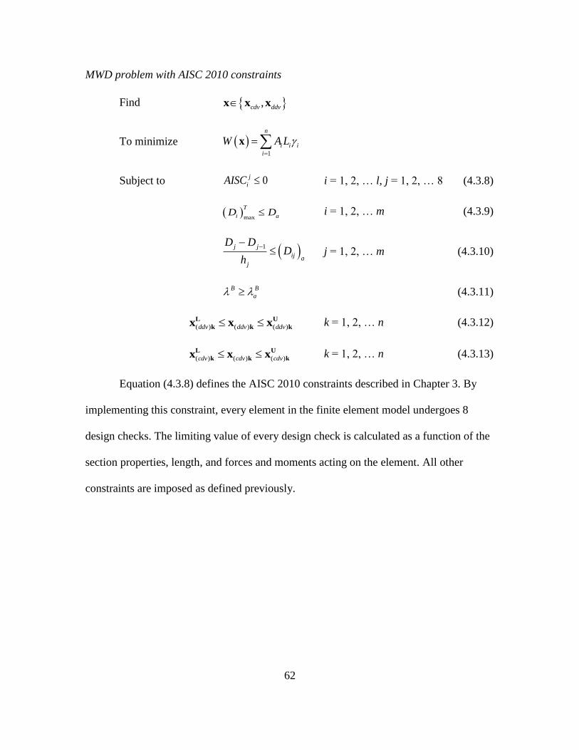
Equation (4.3.8) defines the AISC 2010 constraints described in Chapter 3. By
implementing this constraint, every element in the finite element model undergoes 8
design checks. The limiting value of every design check is calculated as a function of the
section properties, length, and forces and moments acting on the element. All other
constraints are imposed as defined previously.

63
5 VALIDATION OF FEA (with ABAQUS)
Before we proceed to case studies for studying the techniques discussed earlier in
this dissertation, it is necessary to validate Frame3D results. For this purpose, results
from Frame3D of a few models are compared with those from Abaqus. Types of analyses
being verified include stress (static) analysis and modal (frequency) analysis. Responses
from the following planar and 3D models are compared using Frame3D (V 2.83) and
Abaqus (6.11-1).
40S-PL_Bay1 40S-PL_DG 40S-PL_FT 40S-PL_Pyramid
Figure 5.1 Models for validation of Frame3D

64
5.1 Static Analysis
Since it is not feasible to include results for all nodes and elements from all the
models, results in the form of highest values of nodal displacements (which occur at the
topmost point in a structure), nodal reactions at two nodes, and randomly selected
elements for beam element forces & moments are being observed. Results from load
cases (i) dead load + live load (LC1) and (ii) dead, live + 0.6 wind loads (LC4) are being
compared. Following tables illustrate the observations.

65
Displacement comparison - Load case 1 - Dead load + Live load
Model Name Node
Abaqus Frame3D
X-Disp Z-Disp Y-Rot X-Disp Z-Disp Y-Rot
in in rad in in rad
40S-PL-DV+CV-
D+L+W_AISC_Bay1
41-7 -7.96E-02 -3.35 -2.21E-03 -7.96E-02 -3.35 -2.20E-03
41-1 7.96E-02 -3.35 2.21E-03 7.96E-02 -3.35 2.20E-03
40S-PL-DV+CV-
D+L+W_AISC_DG
41-7 1.99E-02 -3.10 1.72E-03 1.99E-02 -3.10 1.72E-03
41-1 -1.93E-02 -3.10 -1.72E-03 -1.93E-02 -3.10 -1.72E-03
40S-PL-DV+CV-
D+L+W_AISC_FT
41-7 2.23E-02 -3.21 3.74E-03 -2.23E-02 -3.21 -3.73E-03
41-1 -2.23E-02 -3.21 -3.74E-03 2.23E-02 -3.21 3.73E-03
40S-PL-DV+CV-
D+L+W_AISC_Pyr
41-7 3.76E-02 -3.15 8.26E-04 -3.76E-02 -3.15 -8.26E-04
41-1 -3.75E-02 -3.15 -8.26E-04 3.76E-02 -3.15 8.26E-04
Table 5.1 Nodal displacements – LC1
Displacement comparison - Load case 2 - Dead load + 0.6 wind load
Model Name Node
Abaqus Frame3D
X-Disp Z-Disp Y-Rot X-Disp Z-Disp Y-Rot
in in rad in in rad
40S-PL-DV+CV-
D+L+W_AISC_Bay1
41-7 1.02E+01 -2.33 1.65E-04 1.01E+01 -2.33 1.65E-04
41-1 1.02E+01 -1.30 2.48E-03 1.02E+01 -1.30 2.48E-03
40S-PL-DV+CV-
D+L+W_AISC_DG
41-7 4.10E+00 -2.08 -3.53E-04 4.10E+00 -2.08 -3.50E-04
41-1 4.12E+00 -1.29 1.43E-03 4.12E+00 -1.29 1.43E-03
40S-PL-DV+CV-
D+L+W_AISC_FT
41-7 4.69E+00 -1.29 2.99E-03 4.69E+00 -1.29 2.98E-03
41-1 4.67E+00 -2.23 -1.33E-03 4.67E+00 -2.23 -1.33E-03
40S-PL-DV+CV-
D+L+W_AISC_Pyr
41-7 8.39E+00 -2.18 2.62E-04 8.38E+00 -2.18 2.62E-04
41-1 8.43E+00 -1.24 1.13E-03 8.42E+00 -1.24 1.13E-03
Table 5.2 Nodal displacements – LC4

66
Table 5.3 Nodal reactions – LC1
Table 5.4 Nodal reactions – LC4
Reaction comparison - Load case 1 - Dead load + live load
Model Name Node
Abaqus Frame3D
X-Force Z-Force Y-Mom X-Force Z-Force Y-Mom
lb lb lb-in lb lb lb-in
40S-PL-
AISC_Bay1
1 9.09E+03 1.89E+06 7.48E+05 9.10E+03 1.89E+06 7.50E+05
2 -1.58E+04 2.25E+06 2.03E+05 -1.58E+04 2.25E+06 2.03E+05
40S-PL-
AISC_DG
1 1.52E+03 1.84E+06 1.28E+06 1.53E+03 1.84E+06 1.28E+06
2 4.11E+04 2.40E+06 9.29E+05 4.11E+04 2.40E+06 9.32E+05
40S-PL-
AISC_FT
1 1.88E+05 2.10E+06 2.03E+05 1.88E+05 2.10E+06 9.18E+04
2 -3.51E+02 2.19E+06 1.29E+04 -3.49E+02 2.19E+06 1.31E+04
40S-PL-
AISC_Pyr
1 2.08E+04 1.83E+06 2.20E+06 2.08E+04 1.83E+06 2.20E+06
2 -4.80E+04 2.25E+06 3.53E+05 -4.80E+04 2.25E+06 3.53E+05
Reaction comparison - Load case 4 - Dead load + 0.6 wind load
Model Name Node
Abaqus Frame3D
X-Force Z-Force Y-Mom X-Force Z-Force Y-Mom
lb lb lb-in lb lb lb-in
40S-PL-
AISC_Bay1
1 -2.49E+04 4.22E+05 -4.30E+06 -2.49E+04 4.22E+05 -4.31E+06
2 -5.73E+04 1.32E+06 -5.05E+06 -5.73E+04 1.32E+06 -5.06E+06
40S-PL-
AISC_DG
1 -1.07E+04 5.75E+05 -2.66E+06 -1.08E+04 5.75E+05 -2.66E+06
2 -5.26E+04 1.07E+06 -2.87E+06 -5.26E+04 1.07E+06 -2.88E+06
40S-PL-
AISC_FT
1 -5.58E+03 6.31E+05 -2.05E+06 -5.42E+03 6.31E+05 -2.06E+06
2 -1.00E+04 1.06E+06 -2.02E+06 -1.00E+04 1.06E+06 -2.02E+06
40S-PL-
AISC_Pyr
1 -6.86E+02 2.68E+05 -2.11E+06 -6.74E+02 2.69E+05 -2.11E+06
2 -8.27E+04 1.43E+06 -4.69E+06 -8.27E+04 1.43E+06 -4.70E+06

67
Axial force and moment - Load case 1 - Dead load + live load
Model
Name Element Node
Abaqus Frame3D
Axial Z-Moment Axial Z-
Moment
lb lb-in lb lb-in
40S-
PL_AISC_
Bay1
1C-1 7 -1.89E+06 7.48E+05 1.89E+06 7.50E+05
84 -1.89E+06 -9.97E+05 -1.89E+06 9.97E+05
1C-7 1 -1.89E+06 -7.48E+05 1.89E+06 -7.50E+05
78 -1.89E+06 9.97E+05 -1.89E+06 -9.97E+05
40S-
PL_AISC_
DG
1C-1 7 -1.84E+06 1.28E+06 1.84E+06 1.28E+06
84 -1.84E+06 9.92E+05 -1.84E+06 -9.92E+05
1C-7 1 -1.84E+06 -1.28E+06 1.84E+06 -1.28E+06
78 -1.84E+06 -9.91E+05 -1.84E+06 9.92E+05
40S-
PL_AISC_
FT
1C-1 7 -1.89E+06 5.41E+05 1.89E+06 5.42E+05
84 -1.89E+06 -8.16E+05 -1.89E+06 8.16E+05
1C-7 1 -1.89E+06 -5.41E+05 1.89E+06 -5.42E+05
78 -1.89E+06 8.16E+05 -1.89E+06 -8.16E+05
40S-
PL_AISC_
Pyramid
1C-1 7 -1.83E+06 -2.20E+06 1.83E+06 2.20E+06
84 -1.82E+06 1.79E+06 -1.82E+06 1.80E+06
1C-7 1 -1.83E+06 2.20E+06 1.83E+06 -2.20E+06
78 -1.82E+06 -1.79E+06 -1.82E+06 -1.80E+06
Table 5.5 Beam forces and moments – LC1

68
Axial force and moment - Load case 2 - Dead load + 0.6 wind load
Model
Name Element Node
Abaqus Frame3D
Axial Z-Moment Axial Z-
Moment
lb lb-in lb lb-in
40S-
PL_AISC_
Bay1
1C-1 7 -4.22E+05 4.24E+06 4.22E+05 -4.31E+06
84 -4.16E+05 -1.67E+05 -4.16E+05 -1.00E+05
1C-7 1 -1.67E+06 5.04E+06 1.67E+06 -5.11E+06
78 -1.67E+06 -1.24E+06 -1.67E+06 -1.17E+06
40S-
PL_AISC_
DG
1C-1 7 -5.75E+05 2.60E+06 5.75E+05 -2.66E+06
84 -5.69E+05 9.01E+05 -5.69E+05 9.64E+05
1C-7 1 -1.46E+06 3.98E+06 1.46E+06 -4.05E+06
78 -1.46E+06 2.03E+06 -1.46E+06 2.09E+06
40S-
PL_AISC_
FT
1C-1 7 -6.28E+05 1.55E+06 6.27E+05 -1.62E+06
84 -6.22E+05 8.74E+05 -6.22E+05 9.38E+05
1C-7 1 -1.48E+06 2.12E+06 1.48E+06 -2.19E+06
78 -1.48E+06 1.06E+04 -1.48E+06 7.38E+04
40S-
PL_AISC_
Pyramid
1C-1 7 -2.68E+05 2.05E+06 2.69E+05 -2.11E+06
84 -2.62E+05 2.29E+06 -2.63E+05 2.35E+06
1C-7 1 -1.75E+06 4.45E+06 1.75E+06 -4.52E+06
78 -1.75E+06 3.42E+05 -1.75E+06 4.06E+05
Table 5.6 Beam forces and moments – LC4
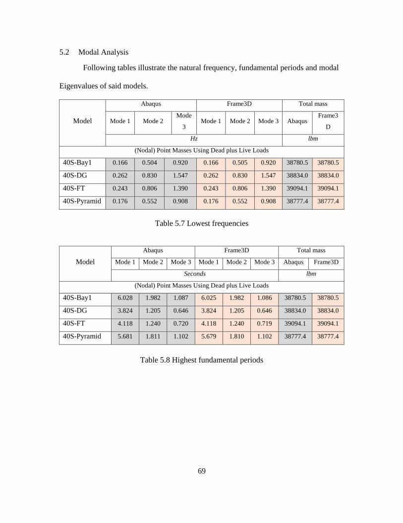
69
5.2 Modal Analysis
Following tables illustrate the natural frequency, fundamental periods and modal
Eigenvalues of said models.
Model
Abaqus Frame3D Total mass
Mode 1 Mode 2 Mode
3 Mode 1 Mode 2 Mode 3 Abaqus
Frame3
D
Hz lbm
(Nodal) Point Masses Using Dead plus Live Loads
40S-Bay1 0.166 0.504 0.920 0.166 0.505 0.920 38780.5 38780.5
40S-DG 0.262 0.830 1.547 0.262 0.830 1.547 38834.0 38834.0
40S-FT 0.243 0.806 1.390 0.243 0.806 1.390 39094.1 39094.1
40S-Pyramid 0.176 0.552 0.908 0.176 0.552 0.908 38777.4 38777.4
Table 5.7 Lowest frequencies
Model
Abaqus Frame3D Total mass
Mode 1 Mode 2 Mode 3 Mode 1 Mode 2 Mode 3 Abaqus Frame3D
Seconds lbm
(Nodal) Point Masses Using Dead plus Live Loads
40S-Bay1 6.028 1.982 1.087 6.025 1.982 1.086 38780.5 38780.5
40S-DG 3.824 1.205 0.646 3.824 1.205 0.646 38834.0 38834.0
40S-FT 4.118 1.240 0.720 4.118 1.240 0.719 39094.1 39094.1
40S-Pyramid 5.681 1.811 1.102 5.679 1.810 1.102 38777.4 38777.4
Table 5.8 Highest fundamental periods

70
Model
Abaqus Frame3D
Modal Eigenvalues
1 2 3 1 2 3
(Nodal) Point Masses Using Dead plus Live Loads
40S-Bay1 1.086 10.045 33.419 1.087 10.054 33.448
40S-DG 2.700 27.188 94.496 2.700 27.187 94.498
40S-FT 2.328 25.668 76.237 2.328 25.671 76.281
40S-Pyramid 1.223 12.041 32.514 1.224 12.047 32.529
Table 5.9 Modal Eigenvalues
It is observed that all the three types of analyses results are in close agreement
with Abaqus results. Highest variation in any type of results is observed to be less than
1%.

71
5.3 Redundancy of Nonlinear Geometric Analysis
All the models being analyzed and/or designed in this dissertation, with strength
based constraints and with AISC 2010 constraints, stresses in all elements are within the
elastic limit of the material. Since the inelastic behavior of the material is not being
considered it is not required to perform a nonlinear geometric analysis. Moreover, since
all the displacements are within the specified limits, this also adds to unnecessity of
nonlinear geometry.

72
6 DESIGN OPTIMIZATION CASE STUDIES
6.1 Finite Element Model
All design models are constructed using a three dimensional, two node beam
element formulation with six independent degrees of freedom (three translations and
three rotations) at each end node of the element. All beams, columns and bracings are
modelled using this type of element. Frame3D uses a 3rd node to define the orientation of
the cross section of the said beam element. Following figures show the degrees of
freedom in local coordinate system in a typical beam element and usage of a 3rd node to
define orientation. All structures are being modelled in US customary units [Units – lb,
lbm, in, psi].
Figure 6.1 Space beam element description and
orientation using a 3rd node

73
Frame3D computer program is employed so as to carry out static analysis,
Eigenvalue buckling analysis, modal analysis and optimal design (using stated analyses)
of interior and exterior planar frames of a square-in-plan building, utilizing only beam
elements. A basic flowchart of the design process implemented in the Frame3D program,
is shown below.
Figure 6.2 Flowchart of the design process
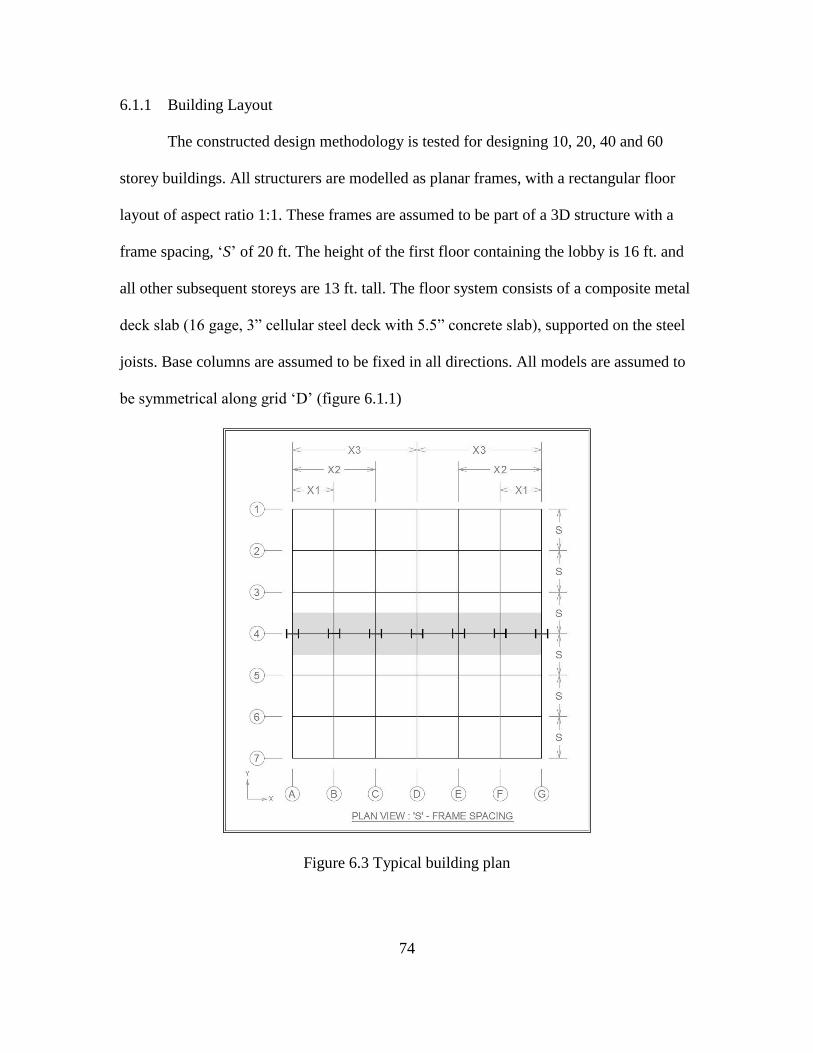
74
6.1.1 Building Layout
The constructed design methodology is tested for designing 10, 20, 40 and 60
storey buildings. All structurers are modelled as planar frames, with a rectangular floor
layout of aspect ratio 1:1. These frames are assumed to be part of a 3D structure with a
frame spacing, ‘S’ of 20 ft. The height of the first floor containing the lobby is 16 ft. and
all other subsequent storeys are 13 ft. tall. The floor system consists of a composite metal
deck slab (16 gage, 3” cellular steel deck with 5.5” concrete slab), supported on the steel
joists. Base columns are assumed to be fixed in all directions. All models are assumed to
be symmetrical along grid ‘D’ (figure 6.1.1)
Figure 6.3 Typical building plan

75
As it was observed in both interior and exterior cases, the extreme end columns
were controlling the design and the interior columns were not being utilized fully. To put
it in other words, extreme end columns could be designed differently (using a different
design variable). But this resulted in increase in the number of design variables and hence
increase in the required design duration. Observing that there was already a heavier
design available for a lower storey interior column, the exterior columns were modelled
same as the interior columns of a group below. Only the columns of bottommost two
storeys were typical throughout the floor. This idea is illustrated in figure 6.1.2.
Figure 6.4 Typical elevation of an interior frame
(2010 – AISC constraints, SB – strength based design)
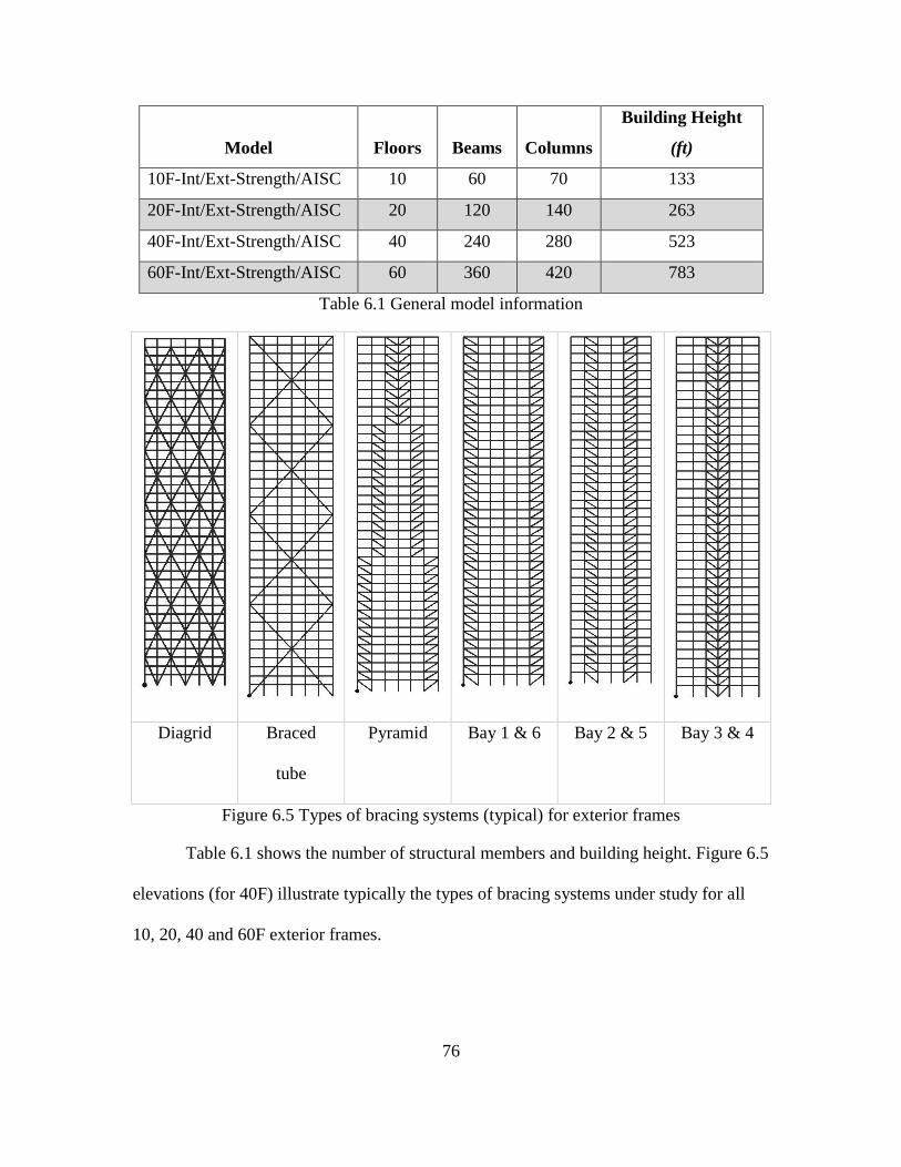
76
Model Floors Beams Columns
Building Height
(ft)
10F-Int/Ext-Strength/AISC 10 60 70 133
20F-Int/Ext-Strength/AISC 20 120 140 263
40F-Int/Ext-Strength/AISC 40 240 280 523
60F-Int/Ext-Strength/AISC 60 360 420 783
Table 6.1 General model information
Diagrid Braced
tube
Pyramid Bay 1 & 6 Bay 2 & 5 Bay 3 & 4
Figure 6.5 Types of bracing systems (typical) for exterior frames
Table 6.1 shows the number of structural members and building height. Figure 6.5
elevations (for 40F) illustrate typically the types of bracing systems under study for all
10, 20, 40 and 60F exterior frames.

77
6.2 Nomenclature and bracing systems
As mentioned earlier, interior and exterior planar frames of four models are being
designed. For every two storeys, there is one column design variable. For example,
element property tag for columns of 3rd and 4th storey will be ‘c3_4’. For beam elements,
the grouping is done bay-wise. There are 6 symmetrical bays present in all models, this
results in 3 bay groups. In the cases of 10F, 20F and 40F models, one variable for one
bay and three stories is being defined and that in 60F models, one variable per bay and 4
stories. For example, in a 20F model, there are 5 groups storey-wise and 3 groups bay-
wise. ‘b2_5’ implies that this variable is defined for second bay, storey-wise 5th group.
All these variables are of discrete type.
As seen in figure 6.1.3, there are two shape variables in a model, namely X1 and
X2. These are continuous design variables, which represent the spans of the bays. X1 is
allowed to vary from 192 to 288 in and X2 from 432 to 528 in. Initially, these variables
are given a value of 240 and 480 in, respectively. As it is a common practice for
outermost bays to be wider than the internal bays, a constraint defining this property is
also being implemented.
As far as bracing systems for exterior frames are concerned, 6 different types are
being studied, namely, Diagrid, Framed Tube, Pyramid type bracing, bay 1 & 6 full, bay
2 & 5 full and bay 3 & 4 all stories braced. Kyoung Sun Moon [10] carried out a study on
Diagrids and Framed Tube bracing system. It was observed that optimum angles for
structures up to 50 stories for diagrid elements is 63° from horizontal and that for
structures higher that 50 stories, was found to be 69°. This was achieved by creating
diagrid elements for every 3 stories in the case of 10, 20 and 40 storied models and in the

78
case of 60 storey, for every 4 stories. It should be noted that since performance of diagrid
systems is a function of the angle formed by diagrids, shape optimization was not
performed on these systems. They also observed that for framed tube, the optimum angle
was 47°. This was achieved by defining the elements for every 5 stories. For pyramid
type system, the building was necessarily divided in three parts. The bottom third has
bracing elements in the outermost bays, middle third of the height has the bracing
elements in intermediate bays and top third in the central two bays. This was done by
observing the bending moment throughout the height of the structure.
All beam and column elements are named in a self-explanatory fashion, storey
number – beam or column tag – Bay number, e.g. 1-C1, 6-B5 etc. Similarly, the bracing
elements are named as, storey number – bracing tag – positive or negative slope – bay
number. For example, a bracing element in second bay of fifth storey with a positive
slope will have a tag ‘5-x1-2’ and that for a negative sloped element in the same bay is
‘5-x2-2’. Similarly, in diagrid and framed tube systems, level-wise groups are created and
elements are differentiated by ‘closing’ or ‘opening’ elements.

79
6.3 Material Properties and Loads
Materials
The steel columns, beams and bracings of the building are assumed to be of grade
A992/A992M. The floor slabs, although not modelled, are assumed to be of high strength
reinforced concrete. Table 6.3 summarizes the material properties.
Material Structural
element Material Property Value
Steel, Grade
A992
Columns &
Beams
Mass density 500 lb/ft3
Elastic Modulus 29,009,200 psi
Yield stress 50 x 103 psi
Poisson's ratio 0.3
Concrete Floor slabs
Mass density 150 lb/ft3
Elastic Modulus 5.8 x 10⁶ psi
Yield stress 580.184 psi
Poisson's ratio 0.15
Table 6.2 Material properties
Loads
The dead loads on the structure include self-weight of the concrete in floor slabs,
self-weight of floor decks and floor finish loads. Assuming the building is for office use,
the live loads are in accordance with the specifications provided in Table 4-1 of ASCE-7-
10, ‘Minimum Design Loads for Buildings and Other Structures’. The table requires the
loads to be a minimum of 50 psf. All the FE models have been designed for 70 psf. Wind
loading is in accordance with the specifications provided in Chicago Building Code,
Division 16, Table 13-52-310, Minimum Design Wind Pressures. For detailed
interpolation and graphical representation of the said wind loads, please refer Appendix
A. Following table shows the intensities of loading in a typical model.

80
Type Description Intensity
psf
DL
Selfweight of concrete 48.30
Selfweight of floor deck 4.10
Floor finish 21.00
Total (Dead) 73.40
LL ASCE 7-10 - minimum 50 psf 70.00
Total (Dead + live) 143.40
Table 6.3 Dead and live load intensities
Therefore, for a frame span ‘S’ of 20 ft,
UDL intensity on all beams = 143.40 psf. x 20 ft / 12 in
= 239 lb/in
Load combinations
All models are designed for four static Allowable Stress Design (ASD) load
combinations as specified in ASCE 7-10. Following are the load combinations.
1. LC 1 – Dead load + live load
2. LC 2 – Dead load + 0.6 wind load
3. LC 3 – Dead load + 0.75 live load + 0.75(0.6 wind load)
4. LC 4 – 0.6 Dead load + 0.6 wind load
All above load cases are also checked for buckling analysis as described in
section 2.2. Along with above mentioned load cases, one load case of modal analysis is
also being carried out.
For modal analysis, point masses are added for gravity loads (DL+LL) on every
node. The intensity of the gravity loads from Table 6.3.2 is 143.4 psf ~1 psi. Therefore,
the point mass on a particular node is the tributary area covered by that node. Now, since
the tributary area is a function of the nodal coordinates, the point masses are defined as a

81
function of coordinates. Following table shows the point mass calculations. ‘S’ is the
span between frames (240”) and X1, X2, X3 and X4 are nodal x coordinates at the right
end of bay 1, bay 2, bay 3 and bay 4 respectively.
Node Point mass
lbm
1 S (X1) / (2 x 386.4)
2 S (X2) / (2 x 386.4)
3 S (X3 - X1) / (2 x 386.4)
4 S (X4 - X2) / (2 x 386.4)
5 S (X3 - X1) / (2 x 386.4)
6 S (X2) / (2 x 386.4)
7 S (X1) / (2 x 386.4)
Table 6.4 Point mass calculations

82
6.4 Numerical results
6.4.1 General model information
All structures are designed for AISC 2010 constraints as well as for fixed
allowable stresses (strength based design). The general model and design related
information is shown in the following table. As described in chapter 4, all frame models
are designed to minimize the weight as the objective function.
Model
Design Variables
(CDV, DDV
(Beam, Col.,
Bracing))
Number
of
Constra
-ints
Best
performing
model
Pop.
Size
Time
for 100
FE (s)
10F-Int-SBD 0, 17 (12, 5, 0) 2218 Sizing 170 1.8
20F-Int-SBD 2, 25 (15, 10, 0) 5819 Sizing + Shape 270 3.8
40F-Int-SBD 2, 62 (42, 20, 0) 8698 Sizing + Shape 640 7.6
60F-Int-SBD 0, 75 (45, 30, 0) 13016 Sizing + Shape 750 11.8
10F-Int-AISC 2, 17 (12, 5, 0) 4819 Sizing + Shape 190 2.1
20F-Int-AISC 2, 25 (15, 10, 0) 9579 Sizing + Shape 270 4.1
40F-Int-AISC 2, 62 (42, 20, 0) 19099 Sizing + Shape 640 8.6
60F-Int-AISC 2, 75 (45, 30, 0) 28618 Sizing + Shape 770 13.6
10F-Ext-SBD 2, 19 (12, 5, 2) 2266 Framed Tube 210 1.8
20F-Ext-SBD 0, 31 (15, 10, 6) 4811 Diagrid 310 3.9
40F-Ext-SBD 2, 70 (42, 20, 8) 8888 Framed Tube 720 8.0
60F-Ext-SBD 0, 95 (45, 30, 20) 14459 Diagrid 950 12.5
10F-Ext-AISC 2, 19 (12, 5, 2) 5459 Pyramid 210 2.3
20F-Ext-AISC 0, 31 (15, 10, 6) 10859 Pyramid 310 4.7
40F-Ext-AISC 2, 70 (42, 20, 8) 21659 Pyramid 720 9.6
60F-Ext-AISC 2, 105 (45, 30, 30) 32459 Diagrid 1070 15.9
Table 6.5 General design related information
The design variables are of two types, viz., CDV and DDV. The first number
denotes the number of CDVs and second denoted DDVs. The parenthesis shows the
breakdown of DDVs – number of beam DDVs, number of column DDVs and number of
bracing DDVs.

83
Although, design process was carried out for all previously described exterior
frames, results are being discussed only for the ‘best performing’ models. The
performance is quantified solely based on the resultant weight of the frame. It is observed
with AISC constraints that exterior frames with pyramid type of bracing system performs
better than all up to 40F models. And with 60F model, diagrid resulted in lowest weight.
This is necessarily due to shorter length of the bracing members as compared to diagrid
and framed tube systems.
As it should be, the time required per function evaluation (FE) grows
exponentially with a linear increase in building. The population size is 10 times the
number of design variables.
6.4.2 Design properties
As seen in table 6.6, for most of the planar frames, LC3 – D + 0.75L + 0.45W is
the controlling load case. Meaning, one of the variables is being utilized most in this
particular load case. Although LC3 seems to be controlling, LC2 – D + 0.6L results in
most of variables reaching high utilization as the story height increases and the wind load
becomes dominant. Typically, wind load is observed to be rather dormant in 10F and 20F
structures. This is due to low intensity of WL for lower heights. Please refer Appendix A
for the overall intensities of wind loads according to Chicago Building Code. For these
models, LC1 – D + L results in high utilization of most variables.

84
Model Design Controlled By
Smallest
Buckling
Factor
Highest
Period
(s)
Max.
Lateral
Disp
(in)
10F-Int-SBD Comp. 1-C5 (D+0.75L +0.45W) 14.6 2.8 2.5
20F-Int-SBD Tens. 9-B5 (D+0.75L +0.45W) 11.7 4.2 6.0
40F-Int-SBD Disp. 41-1 (D+0.6W) 16.0 5.4 12.5
60F-Int-SBD Comp. 15-C6 (D+0.75L +0.45W) 21.7 6.0 18.6
10F-Int-AISC Comp. + Bend. 10-B1 (D+L) 15.4 2.6 2.1
20F-Int-AISC Disp. 21-1 (D + 0.6W) 9.8 3.8 6.3
40F-Int-AISC Comp. + Bend. 3-C4 (D+L) 14.5 5.4 12.1
60F-Int-AISC Comp. + Bend. 29-C7 (D+0.75L +0.45W) 23.9 6.1 17.7
10F-Ext-SBD Tens. 5-B5 (D+L) 28.0 1.4 0.7
20F-Ext-SBD Comp. 5-C3 (D+L) 17.7 2.2 2.4
40F-Ext-SBD Comp. 7XC2 (D+0.75L+0.45W) 23.7 4.5 8.5
60F-Ext-SBD Comp. 7XO5 (D+0.75L+0.45W) 22.3 4.9 17.9
10F-Ext-AISC Tens. + Bend. 7-B3 (D+L) 29.3 1.5 0.8
20F-Ext-AISC Comp. + Bend. 7-C2 (D+L) 21.3 2.5 2.5
40F-Ext-AISC Comp. + Bend. 14-C6 (D+0.75L+0.45W) 15.2 4.6 10.8
60F-Ext-AISC Tens. + Bend. 45-B4 (D+L) 28.5 5.0 12.5
Table 6.6 Controlling factors and design properties
It is observed in the AISC models that columns are being utilized fully but beam
elements are not. As seen in table 6.6, combined effect of compression and bending is the
limit state for which, most of the models are designed. The primary function of the beam
elements shifts from just carrying the loads to providing the complementary moment of
inertia to provide rotational stiffness to the column elements, as the building height
increases. This is necessarily to increase the degree of fixity for columns, which results in
increased buckling strength and allows for the columns to be designed in the limit state of
yielding. Unnecessary to mention, limit state of yielding results in higher load carrying
capacity as compared to any other limit states in compression design (refer section 3.1.2).

85
As stated in section 3.1.2, the structure needs to designed in such a manner that
the lowest Eigenvalue should be greater than 1 in order to bypass the limit state of
flexural buckling. The buckling analyses carried out on the designed structures satisfy
this criterion by a huge margin.
Figure 6.6 Highest period vs building height
In both, internal ‘rigid’ frames and external braced frames, it is observed that
highest natural period of the frames appear to be converging. Bracing systems help to
enhance the modal performance of the frames. Also, SB internal frames perform almost
hand in hand with AISC internal frames. This is also true for external frames. The best
performing model in the case if strength based external frames for 40F models is Framed
Tube, whereas in the case of AISC based 40F, Pyramid type bracings perform better. As
far as modal performance is concerned, Diagrid and Framed tube systems outperformed
1.0
2.0
3.0
4.0
5.0
6.0
7.0
0 100 200 300 400 500 600 700 800
Na
tura
l Per
iod
(s)
Height (ft)
Highest Period vs Building Height
SB Int. Norm. Highest Period
AISC Int. Norm. Highest Period
SB Ext. Norm. Highest Period
AISC Ext. Norm. Highest Period

86
any other type. On an average, Diagrid and Framed tube systems provide 30-40% lower
highest periods as compared to the next best Pyramid systems.
6.4.3 Weight performance
In both internal and external models and in both SB and AISC based designs,
beam weight contribution towards the entire structures weight gradually decreases as the
height of the building increases. For 10F models, the beam weight contribution ranges
from 40-50%, and that reduces to 12-20% in the case of 60F models.
In general, columns are designed heavier with the AISC constraints as compared
to strength based models. This is due to allowable compressive stresses in SB designs are
30 ksi, and that with AISC constraints works out to be 22.5 ksi. It should be noted that
this allowable value varies as a function of length of the member, section dimensions etc.
in accordance with AISC limit states. As a result, the weight contribution of beams is
lower in most cases of AISC based designs.
The normalized weight (weight per designed unit area) is computed by assuming
a square building with 14 frames as
, , , , .
2
2 45 5 5 4 4
7 7
(36 )
Int Int Beam Int Col Ext Beam Ext Col Brac
N
Stories
W W W W W W
WN S
(6.5)
Where, WInt is the weight of the interior frame, WExt is the weight of the exterior
frame and NStories is the number of stories in the structure. It should be noted that the
weight is calculated center-to-center without accounting for connections.

87
In the normalized weight calculations, only the weight of structural steel elements
(beams, columns and bracing members) are included. Following table illustrate weight
performance from the optimization results.
Model
Beam
weight
(ton)
Column
weight
(ton)
Bracing
weight
(ton)
Total
weight
(ton)
Beam
weight
(%)
Normalized
weight (psf)
10F-Int-SBD 25.1 24.1 - 49.2 51.0
Calculated
for
combined
internal +
external
frames
20F-Int-SBD 53.0 83.1 - 136.1 38.9
40F-Int-SBD 176.5 355.3 - 531.8 33.2
60F-Int-SBD 481.6 808.5 - 1290.1 37.3
10F-Int-AISC 25.6 29.7 - 55.3 46.3
20F-Int-AISC 59.2 97.5 - 156.7 37.8
40F-Int-AISC 192.7 391.7 - 584.4 33.0
60F-Int-AISC 459.1 884.5 - 1343.6 34.2
10F-Ext-SBD 21.5 22.4 2.9 46.8 45.9 7.2
20F-Ext-SBD 48.5 68.9 14.4 134.6 36.0 9.4
40F-Ext-SBD 130.7 304.8 18.4 453.8 28.8 16.7
60F-Ext-SBD 196.7 749.4 94.1 1040.1 18.9 26.9
10F-Ext-AISC 20.1 27.9 2.6 50.6 39.7 7.7
20F-Ext-AISC 45.4 99.2 8 152.6 29.8 10.3
40F-Ext-AISC 128.3 347.1 23.1 498.4 25.7 18.2
60F-Ext-AISC 122.9 804.6 146 1073.4 11.4 27.3
Table 6.7 Weight performance from optimization results
As mentioned by Ali and Moon[5], there is a premium for height for taller
structures due to lateral loads. As a result, total structural material consumption increases
exponentially with a linear increase of height. This effect can be clearly seen from table
6.7 and figure 6.7.

88
Figure 6.7 Normalized weight vs Building height
In figure 6.7, it can be seen that despite the fact that the bracing systems varies
throughout the SB models, the plots for normalized weights of SB and AISC based
models are parallel. The exponential nature of the plots can be clearly seen in these plots.
As a general observation and according to the allowable stress value calculations, AISC
based designs are, on an average, 7% heavier as compared to strength based designs.
A regression analysis was carried out on both the curves. Curve for models with
strength based constraints follow the equation
Nw [SB] = 5.71 e1.988E-03 (Height)
And curve for models with AISC constraints follow the equation
Nw [AISC] = 6.501 e1.85E-03 (Height)
Where, Nw is in psf and Height is in ft.
1.0
6.0
11.0
16.0
21.0
26.0
31.0
0 100 200 300 400 500 600 700 800
No
rma
lized
Wei
gh
t (p
sf)
Height (ft)
Normalized weight vs Building Height
SBDAISCD

89
7 CONCLUSIONS
This thesis presents a design methodology in accordance with AISC Steel
Construction Manual 2010 Specifications. An algorithm has been developed for I-
sections and implemented in GS-USA Frame3D program.
One of the most tedious tasks in these design checks is to compute the ‘K’ factors
for compression members in the limit state of flexural buckling. One of the provisions to
bypass these calculations for every compression member in a finite element model is
described in section E3 and Appendix 7, Section 7.2.3(b). This provision needs a
satisfactory side-sway buckling analysis in order to bypass these calculations. This
provision has been developed in the algorithm and implemented in Frame3D program.
This work also concentrates on structural design optimization of interior and
exterior planar frames of ten, twenty, forty and sixty storey buildings. For exterior
frames, six different types of bracing systems are designed and optimized for all four
buildings. All models are optimized with AISC 2010 constraints as well as strength based
constraints (as separate finite element models) for comparison purposes. Also, lateral
deflection, inter-story drift and Euler buckling constraints are enforced in all models.
A database of 189 selective W shapes was extracted out of all 273 AISC standard
sections. These sections have a higher moment of inertia to c/s area ratio as compared to
the rest 84 discarded sections. In order to be able to use gradient-based optimization
technique of MFD, a satisfactory regression analysis was performed to obtain the
relationships between c/s area and general properties of the section. Following are the key
features of the optimization results –
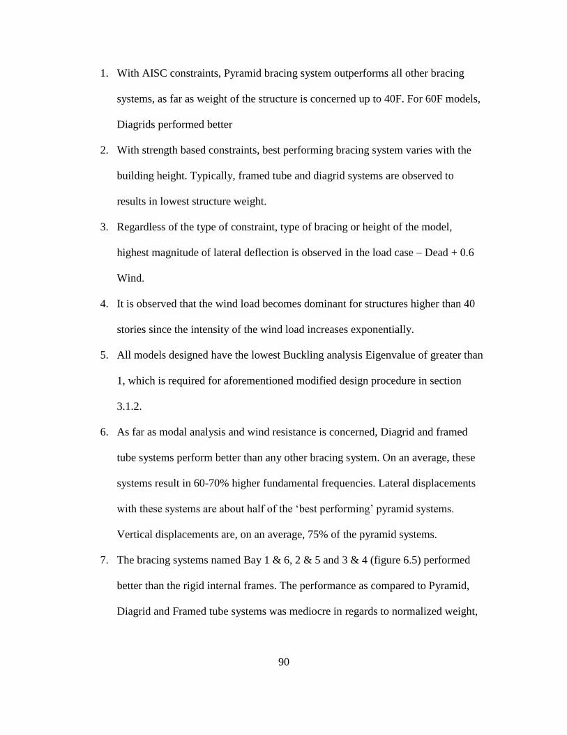
90
1. With AISC constraints, Pyramid bracing system outperforms all other bracing
systems, as far as weight of the structure is concerned up to 40F. For 60F models,
Diagrids performed better
2. With strength based constraints, best performing bracing system varies with the
building height. Typically, framed tube and diagrid systems are observed to
results in lowest structure weight.
3. Regardless of the type of constraint, type of bracing or height of the model,
highest magnitude of lateral deflection is observed in the load case – Dead + 0.6
Wind.
4. It is observed that the wind load becomes dominant for structures higher than 40
stories since the intensity of the wind load increases exponentially.
5. All models designed have the lowest Buckling analysis Eigenvalue of greater than
1, which is required for aforementioned modified design procedure in section
3.1.2.
6. As far as modal analysis and wind resistance is concerned, Diagrid and framed
tube systems perform better than any other bracing system. On an average, these
systems result in 60-70% higher fundamental frequencies. Lateral displacements
with these systems are about half of the ‘best performing’ pyramid systems.
Vertical displacements are, on an average, 75% of the pyramid systems.
7. The bracing systems named Bay 1 & 6, 2 & 5 and 3 & 4 (figure 6.5) performed
better than the rigid internal frames. The performance as compared to Pyramid,
Diagrid and Framed tube systems was mediocre in regards to normalized weight,

91
lateral and vertical deflections, highest period and Buckling Eigenvalues for all
the four exterior frame model heights.
8. It is observed that there is a gradual decrease in the beam weight contribution as
the height of the structure increases. It drops from 40-50% in 10F models to
around 12% in 60F models.
9. Columns in the models with AISC constraints require heavier sections as
compared to strength based design models. Also, in almost all the models, the
column elements have a higher utility ratio as compared to beam utility ratio.
10. The AISC constraint based models are designed 10% heavier (normalized steel
consumption) on an average as compared to strength based models.
11. As established by Dr. Fazlur Khan, there exists a ‘premium for height’. The
normalized structural steel consumption increases exponentially with a linear
increase in height of the structure.
92
REFERENCES
[1] Victor E. Saouma, "lecture notes in structural engineering", University of Colorado,
2007.
[2] "ETABS receives ‘Top Seismic Product of the 20th Century’ Award", Press release.
Structure magazine, 2006.
[3] Baker, William F., "Structural Innovation", Tall buildings and urban habitat: cities in
the third millennium, New York: Spon Press. pp. 481–493. ISBN 0-415-23241-4, 2001.
[4] Bayley, Stephen, "Burj Dubai: The new pinnacle of vanity", Telegraph (London),
2010.
[5] Ali and Moon, “Structural developments in tall buildings: Current trends and future
prospects”, Architectural Science Review, Vol. 50.3, pp 205-223, 2007.
[6] S. D. Rajan, “Introduction to Structural Analysis and Design”, Wiley, 2013.
[7] David S. Burnett, “Finite Element Analysis: From Concepts to Applications”,
Addison-Wesley, 1988.
[8] William McGuire, Richard H. Gallagher and Ronald D. Ziemian, “Matrix Structural
Analysis, Second Edition”, Section 12.8, pp 360.
[9] Jack C. McCormac, “Structural Steel Design, Second Edition”, Section 18-9 Flexure-
shear interaction, pp. 605.
[10] Kyoung Sun Moon, “Material-Saving Design Strategies for Tall Building
Structures”, CTBUH 2008 8th World Congress, Dubai, 2008.
[11] C. M. Chan, D. E. Grierson and N. Sherbourne, “Automatic Optimal Design of Tall
Steel Building Frameworks”.
93
APPENDIX A
DESIGN WIND LOADS DERIVED FROM CHICAGO BUILDING CODE, DIV. 16,
TABLE 13-52-310

94
Storey
Height Wind Pressure
Storey
Height Wind Pressure
(ft) Nodal
load (psf)
Nodal
load (lb) (ft)
Nodal
load (psf)
Nodal
load (lb)
1 16 20.00 33.33 31 406 25.18 41.97
2 29 20.00 33.33 32 419 25.57 42.62
3 42 20.00 33.33 33 432 25.96 43.27
4 55 20.00 33.33 34 445 26.35 43.92
5 68 20.00 33.33 35 458 26.74 44.57
6 81 20.00 33.33 36 471 27.13 45.22
7 94 20.00 33.33 37 484 27.52 45.87
8 107 20.00 33.33 38 497 27.91 46.52
9 120 20.00 33.33 39 510 28.30 47.17
10 133 20.00 33.33 40 523 28.69 47.82
11 146 20.00 33.33 41 536 29.08 48.47
12 159 20.00 33.33 42 549 29.47 49.12
13 172 20.00 33.33 43 562 29.86 49.77
14 185 20.00 33.33 44 575 30.25 50.42
15 198 20.00 33.33 45 588 30.64 51.07
16 211 20.11 33.52 46 601 31.02 51.70
17 224 20.24 33.73 47 614 31.28 52.13
18 237 20.37 33.95 48 627 31.54 52.57
19 250 20.50 34.17 49 640 31.80 53.00
20 263 20.63 34.38 50 653 32.06 53.43
21 276 20.76 34.60 51 666 32.32 53.87
22 289 20.89 34.82 52 679 32.58 54.30
23 302 21.08 35.13 53 692 32.84 54.73
24 315 21.60 36.00 54 705 33.15 55.25
25 328 22.12 36.87 55 718 33.54 55.90
26 341 22.64 37.73 56 731 33.93 56.55
27 354 23.16 38.60 57 744 34.32 57.20
28 367 23.68 39.47 58 757 34.71 57.85
29 380 24.20 40.33 59 770 35.10 58.50
30 393 24.72 41.20 60 783 35.49 59.15

95
0
50
100
150
200
250
300
350
400
450
500
550
600
650
700
750
800
15 20 25 30 35 40
Bu
idin
g h
eigh
t (f
t)
Wind load intensity (psf)
Wind Load Intensity vs. Building Height

96
APPENDIX B
AISC WIDE FLANGE SECTIONS SELECTED IN THE DDV TABLE

97
Symbol Property description
Line Line number in the DDV table
Property Cross section tag for wide flange section
Area Cross sectional area
Iz Moment of inertia about local z axis
Iy Moment of inertia about y axis
J Torsional constant
0.833*Cross sectional area
Sz Section modulus about the local z axis
Sy Section modulus about the local y axis
SFz “Shear factor” for computing shear stress (shear force acting in the local z
direction)
SFy “Shear factor” for computing shear stress (shear force acting in the local y
direction)
TF “Torsional factor” for computing the shear stress due to torsional moment
Line Property Area Iz Iy J Sz Sy SFz SFy TF
1 WF 6x8.5 2.52 14.9 1.99 0.03 5.1 1.01 0.5 0.91 0.15
2 WF 6x9 2.68 16.4 2.2 0.04 5.56 1.11 0.55 0.92 0.18
3 WF 8x10 2.96 30.8 2.09 0.04 7.81 1.06 0.52 1.22 0.18
4 WF 10x12 3.54 53.8 2.18 0.05 10.9 1.1 0.53 1.67 0.23
5 WF 6x12 3.55 22.1 2.99 0.09 7.31 1.5 0.72 1.25 0.31
6 WF 4x13 3.83 11.3 3.86 0.15 5.46 1.9 0.91 1.02 0.42
7 WF 8x13 3.84 39.6 2.73 0.09 9.91 1.37 0.65 1.64 0.31
8 WF 12x14 4.16 88.6 2.36 0.07 14.9 1.19 0.56 2.09 0.29
9 WF 10x15 4.41 68.9 2.89 0.1 13.8 1.45 0.68 2.03 0.37
10 WF 6x15 4.43 29.1 9.32 0.1 9.72 3.11 1.02 1.26 0.37
11 WF 8x15 4.44 48 3.41 0.14 11.8 1.7 0.81 1.77 0.42
12 WF 5x16 4.71 21.4 7.51 0.19 8.55 3 1.19 1.08 0.52
13 WF 12x16 4.71 103 2.82 0.1 17.1 1.41 0.66 2.31 0.38
14 WF 6x16 4.74 32.1 4.43 0.22 10.2 2.2 1.06 1.45 0.57
15 WF 10x17 4.99 81.9 3.56 0.16 16.2 1.78 0.84 2.15 0.48
16 WF 8x18 5.26 61.9 7.97 0.17 15.2 3.04 1.13 1.7 0.52
17 WF 12x19 5.57 130 3.76 0.18 21.3 1.88 0.89 2.5 0.55
18 WF 10x19 5.62 96.3 4.29 0.23 18.8 2.14 1.02 2.28 0.62
19 WF 8x21 6.16 75.3 9.77 0.28 18.2 3.71 1.38 1.87 0.73
20 WF 12x22 6.48 156 4.66 0.29 25.4 2.31 1.09 2.81 0.75
21 WF 10x22 6.49 118 11.4 0.24 23.2 3.97 1.35 2.2 0.69
22 WF 14x22 6.49 199 7 0.21 29 2.8 1.08 2.85 0.61
23 WF 10x26 7.61 144 14.1 0.4 27.9 4.89 1.66 2.43 0.97
24 WF 12x26 7.65 204 17.3 0.3 33.4 5.34 1.61 2.56 0.83
25 WF 16x26 7.68 301 9.59 0.26 38.4 3.49 1.21 3.48 0.76
26 WF 14x26 7.69 245 8.91 0.36 35.3 3.55 1.35 3.18 0.88
27 WF 12x30 8.79 238 20.3 0.46 38.6 6.24 1.87 2.91 1.11
28 WF 10x30 8.84 170 16.7 0.62 32.4 5.75 1.93 2.81 1.31
29 WF 14x30 8.85 291 19.6 0.38 42 5.82 1.69 3.4 0.99

98
Line Property Area Iz Iy J Sz Sy SFz SFy TF
30 WF 16x31 9.13 375 12.4 0.46 47.2 4.49 1.56 3.88 1.1
31 WF 10x33 9.71 171 36.6 0.58 35 9.2 2.28 2.62 1.26
32 WF 14x34 10 340 23.3 0.57 48.6 6.91 1.99 3.6 1.3
33 WF 12x35 10.3 285 24.5 0.74 45.6 7.47 2.23 3.37 1.54
34 WF 18x35 10.3 510 15.3 0.51 57.6 5.12 1.62 4.68 1.24
35 WF 16x36 10.6 448 24.5 0.55 56.5 7 1.95 4.18 1.31
36 WF 14x38 11.2 385 26.7 0.8 54.6 7.88 2.27 3.94 1.63
37 WF 10x39 11.5 209 45 0.98 42.1 11.3 2.78 2.87 1.81
38 WF 12x40 11.7 307 44.1 0.91 51.5 11 2.71 3.25 1.75
39 WF 16x40 11.8 518 28.9 0.79 64.7 8.25 2.29 4.39 1.67
40 WF 18x40 11.8 612 19.1 0.81 68.4 6.35 2.02 4.99 1.68
41 WF 14x43 12.6 428 45.2 1.05 62.6 11.3 2.78 3.84 1.91
42 WF 21x44 13 843 20.7 0.77 81.6 6.37 1.84 6.31 1.7
43 WF 12x45 13.1 348 50 1.26 57.7 12.4 3.04 3.68 2.21
44 WF 10x45 13.3 248 53.4 1.51 49.1 13.3 3.28 3.21 2.44
45 WF 16x45 13.3 586 32.8 1.11 72.7 9.34 2.57 4.98 2.11
46 WF 18x46 13.5 712 22.5 1.22 78.8 7.43 2.34 5.71 2.23
47 WF 14x48 14.1 484 51.4 1.45 70.2 12.8 3.13 4.3 2.4
48 WF 21x48 14.1 959 38.7 0.8 93 9.52 2.24 6.41 1.83
49 WF 10x49 14.4 272 93.4 1.39 54.6 18.7 3.7 3.11 2.45
50 WF 12x50 14.6 391 56.3 1.71 64.2 13.9 3.39 4.09 2.73
51 WF 16x50 14.7 659 37.2 1.52 81 10.5 2.88 5.49 2.62
52 WF 18x50 14.7 800 40.1 1.24 88.9 10.7 2.76 5.69 2.36
53 WF 21x50 14.7 984 24.9 1.14 94.5 7.64 2.2 6.94 2.22
54 WF 12x53 15.6 425 95.8 1.58 70.6 19.2 3.79 3.83 2.66
55 WF 14x53 15.6 541 57.7 1.94 77.8 14.3 3.48 4.71 2.94
56 WF 10x54 15.8 303 103 1.82 60 20.6 4.08 3.42 2.95
57 WF 18x55 16.2 890 44.9 1.66 98.3 11.9 3.06 6.28 2.88
58 WF 21x55 16.2 1140 48.4 1.24 110 11.8 2.76 6.92 2.44
59 WF 24x55 16.2 1350 29.1 1.18 114 8.3 2.21 8.07 2.39
60 WF 21x57 16.7 1170 30.6 1.77 111 9.35 2.69 7.47 2.97
61 WF 16x57 16.8 758 43.1 2.22 92.2 12.1 3.28 6.27 3.39
62 WF 12x58 17 475 107 2.1 78 21.4 4.23 4.04 3.23
63 WF 18x60 17.6 984 50.1 2.17 108 13.3 3.38 6.73 3.44
64 WF 10x60 17.7 341 116 2.48 66.7 23 4.5 3.89 3.67
65 WF 14x61 17.9 640 107 2.19 92.1 21.5 4.22 4.78 3.39
66 WF 24x62 18.2 1550 34.5 1.71 131 9.8 2.6 8.86 3.06
67 WF 21x62 18.3 1330 57.5 1.83 127 14 3.26 7.47 3.16
68 WF 12x65 19.1 533 174 2.18 87.9 29.1 4.79 4.38 3.51
69 WF 18x65 19.1 1070 54.8 2.73 117 14.4 3.66 7.26 4.04
70 WF 16x67 19.6 954 119 2.39 117 23.2 4.5 5.88 3.82
71 WF 10x68 19.9 394 134 3.56 75.7 26.4 5.19 4.4 4.7
72 WF 14x68 20 722 121 3.01 103 24.2 4.77 5.35 4.22
73 WF 21x68 20 1480 64.7 2.45 140 15.7 3.64 8.08 3.85
74 WF 24x68 20.1 1830 70.4 1.87 154 15.7 3.36 8.73 3.37
75 WF 18x71 20.9 1170 60.3 3.49 127 15.8 3.96 8 4.79
76 WF 12x72 21.1 597 195 2.93 97.4 32.4 5.36 4.82 4.31

99
Line Property Area Iz Iy J Sz Sy SFz SFy TF
77 WF 21x73 21.5 1600 70.6 3.02 151 17 3.94 8.57 4.44
78 WF 14x74 21.8 795 134 3.87 112 26.6 5.17 5.76 5.05
79 WF 18x76 22.3 1330 152 2.83 146 27.6 4.93 7.01 4.45
80 WF 24x76 22.4 2100 82.5 2.68 176 18.4 3.93 9.34 4.27
81 WF 16x77 22.6 1110 138 3.57 134 26.9 5.1 6.79 5.05
82 WF 10x77 22.7 455 154 5.11 85.9 30.1 5.84 4.99 6.06
83 WF 12x79 23.2 662 216 3.84 107 35.8 5.84 5.28 5.22
84 WF 14x82 24 881 148 5.07 123 29.3 5.7 6.59 6.09
85 WF 21x83 24.4 1830 81.4 4.34 171 19.5 4.46 9.73 5.7
86 WF 24x84 24.7 2370 94.4 3.7 196 20.9 4.46 10.04 5.28
87 WF 27x84 24.7 2850 106 2.81 213 21.2 4.07 10.88 4.57
88 WF 18x86 25.3 1530 175 4.1 166 31.6 5.57 7.95 5.74
89 WF 12x87 25.6 740 241 5.1 118 39.7 6.51 5.87 6.33
90 WF 16x89 26.2 1300 163 5.45 155 31.4 5.9 7.82 6.77
91 WF 30x90 26.3 3610 115 2.84 245 22.1 4.06 12.24 4.71
92 WF 14x90 26.5 999 362 4.06 143 49.9 6.83 5.7 5.73
93 WF 21x93 27.3 2070 92.9 6.03 192 22.1 4.99 11 7.17
94 WF 27x94 27.6 3270 124 4.03 243 24.8 4.76 11.7 5.79
95 WF 24x94 27.7 2700 109 5.26 222 24 5.09 11.06 6.7
96 WF 18x97 28.5 1750 201 5.86 188 36.1 6.38 8.95 7.29
97 WF 30x99 29 3990 128 3.77 269 24.5 4.41 13.44 5.76
98 WF 16x100 29.4 1490 186 7.73 175 35.7 6.72 8.84 8.55
99 WF 21x101 29.8 2420 248 5.21 227 40.3 6.43 9.61 6.96
100 WF 27x102 30 3620 139 5.28 267 27.8 5.34 12.37 6.92
101 WF 24x103 30.3 3000 119 7.07 245 26.5 5.63 11.9 8.13
102 WF 24x104 30.7 3100 259 4.72 258 40.7 6.18 10.76 6.75
103 WF 18x106 31.1 1910 220 7.48 204 39.4 6.85 9.85 8.66
104 WF 30x108 31.7 4470 146 4.99 299 27.9 5.04 14.3 6.92
105 WF 21x111 32.6 2670 274 6.83 249 44.5 7.08 10.66 8.36
106 WF 27x114 33.6 4080 159 7.33 299 31.5 5.97 13.68 8.68
107 WF 30x116 34.2 4930 164 6.43 329 31.3 5.68 14.92 8.16
108 WF 24x117 34.4 3540 297 6.72 291 46.5 7.08 11.97 8.53
109 WF 33x118 34.7 5900 187 5.3 359 32.6 5.39 15.85 7.44
110 WF 18x119 35.1 2190 253 10.6 231 44.9 7.72 10.97 11.03
111 WF 21x122 35.9 2960 305 8.98 273 49.2 7.75 11.62 10.11
112 WF 30x124 36.5 5360 181 7.99 355 34.4 6.27 15.55 9.39
113 WF 27x129 37.8 4760 184 11.1 345 36.8 7.06 14.89 11.35
114 WF 18x130 38.3 2460 278 14.5 256 49.9 8.65 11.32 13.46
115 WF 33x130 38.3 6710 218 7.37 406 37.9 6.3 16.92 9.22
116 WF 24x131 38.6 4020 340 9.5 329 53 7.97 13.2 10.8
117 WF 21x132 38.8 3220 333 11.3 295 53.5 8.44 12.65 11.86
118 WF 30x132 38.8 5770 196 9.72 380 37.2 6.78 16.47 10.69
119 WF 36x135 39.9 7800 225 7 439 37.7 5.93 18.59 9.17
120 WF 33x141 41.5 7450 246 9.7 448 42.7 7.12 17.82 11.01
121 WF 24x146 43 4580 391 13.4 371 60.5 9.16 14.37 13.54
122 WF 21x147 43.2 3630 376 15.4 329 60.1 9.36 14.06 14.64
123 WF 27x146 43.2 5660 443 11.3 414 63.5 8.83 14.93 12.1

100
Line Property Area Iz Iy J Sz Sy SFz SFy TF
124 WF 30x148 43.6 6680 227 14.5 436 43.3 7.87 17.5 13.9
125 WF 40x149 43.8 9800 229 9.36 513 38.8 6.19 21.43 10.36
126 WF 36x150 44.3 9040 270 10.1 504 45.1 7.15 19.65 11.62
127 WF 33x152 44.9 8160 273 12.4 487 47.2 7.77 18.67 13.05
128 WF 36x160 47 9760 295 12.4 542 49.1 7.81 20.61 13.25
129 WF 27x161 47.6 6310 497 15.1 458 70.9 9.88 16.4 14.74
130 WF 24x162 47.8 5170 443 18.5 414 68.4 10.21 15.61 16.84
131 WF 40x167 49.3 11600 283 14 600 47.9 7.71 22.39 13.64
132 WF 33x169 49.5 9290 310 17.7 549 53.9 8.98 20.02 16.29
133 WF 36x170 50 10500 320 15.1 581 53.2 8.47 21.64 15.09
134 WF 30x173 50.9 8230 598 15.6 541 79.8 10.37 17.92 15.64
135 WF 24x176 51.7 5680 479 23.9 450 74.3 11.2 16.79 19.92
136 WF 27x178 52.5 7020 555 20.1 505 78.8 10.86 18.06 17.97
137 WF 40x183 53.3 13200 331 19.3 675 56 9.09 22.79 16.65
138 WF 36x182 53.6 11300 347 18.5 623 57.6 9.01 23.07 17.39
139 WF 30x191 56.1 9200 673 21 600 89.5 11.65 19.52 19.12
140 WF 36x194 57 12100 375 22.2 664 61.9 9.72 24.42 19.68
141 WF 27x194 57.1 7860 619 27.1 559 88.1 12.3 18.92 21.78
142 WF 40x199 58.8 14900 695 18.3 770 88.2 10.82 22.7 17.36
143 WF 33x201 59.1 11600 749 20.8 686 95.2 11.82 21.71 19.39
144 WF 36x210 61.9 13200 411 28 719 67.5 10.44 26.53 23.16
145 WF 40x211 62.1 15500 390 30.4 786 66.1 10.65 26.21 22.98
146 WF 30x211 62.3 10300 757 28.4 665 100 12.92 21.45 23.46
147 WF 40x215 63.5 16700 803 24.8 859 101 12.55 22.96 21
148 WF 33x221 65.3 12900 840 27.8 759 106 13.07 23.52 23.79
149 WF 44x230 67.8 20800 796 24.9 971 101 12.34 27 22.68
150 WF 36x232 68 15000 468 39.6 809 77.2 12.11 28.19 28.85
151 WF 36x231 68.2 15600 940 28.7 854 114 13.43 24.91 24.25
152 WF 40x235 69.1 17400 444 41.3 875 74.6 11.87 29.06 28.56
153 WF 33x241 71.1 14200 933 36.2 831 118 14.32 25.22 28.31
154 WF 36x247 72.5 16700 1010 34.7 913 123 14.41 26.23 27.59
155 WF 40x249 73.5 19600 926 38.1 993 118 14.42 26.66 28.36
156 WF 36x256 75.3 16800 528 52.9 895 86.5 13.38 31.34 35.3
157 WF 36x262 77.2 17900 1090 41.6 972 132 15.36 27.57 31.29
158 WF 44x262 77.2 24100 923 37.3 1110 117 14.29 30.01 29.84
159 WF 33x263 77.4 15900 1040 48.7 919 131 16.17 26.84 34.27
160 WF 40x264 77.4 19400 493 56.1 971 82.6 13.03 33.61 35.5
161 WF 40x277 81.5 21900 1040 51.5 1100 132 16.15 29.59 35.05
162 WF 40x278 82.3 20500 521 65 1020 87.1 13.47 35.84 39.78
163 WF 36x282 82.9 19600 1200 52.7 1050 144 16.9 29.37 36.55
164 WF 44x290 85.4 27000 1040 50.9 1240 132 16.05 33.3 36.78
165 WF 33x291 85.6 17700 1160 65.1 1020 146 17.77 29.67 41.88
166 WF 40x294 86.2 21900 562 76.6 1080 93.5 14.54 37.3 44.21
167 WF 40x297 87.3 23200 1090 61.2 1170 138 16.82 33.08 39.68
168 WF 36x302 89 21100 1300 64.3 1130 156 18.06 31.36 42.03
169 WF 33x318 93.7 19500 1290 84.4 1110 161 19.47 32.09 50.11
170 WF 40x324 95.3 25600 1220 79.4 1280 153 18.56 35.57 47.52

101
Line Property Area Iz Iy J Sz Sy SFz SFy TF
171 WF 40x327 95.9 24500 640 103 1200 105 16.17 41.58 54.55
172 WF 36x330 96.9 23300 1420 84.3 1240 171 19.92 34.06 50.31
173 WF 40x331 97.7 24700 644 105 1210 106 15.94 42.68 56.09
174 WF 44x335 98.5 31100 1200 74.7 1410 150 18.12 39.79 48.14
175 WF 33x354 104 22000 1460 115 1240 181 21.68 36.1 61.91
176 WF 36x361 106 25700 1570 109 1350 188 21.69 37.59 60.03
177 WF 40x362 106 28900 1380 109 1420 173 20.64 40.07 59.23
178 WF 40x372 110 29600 1420 116 1460 177 20.94 41.4 62.4
179 WF 33x387 114 24300 1620 148 1350 200 23.7 39.33 73.99
180 WF 36x395 116 28500 1750 142 1490 208 23.83 41.13 72.17
181 WF 40x392 116 29900 803 172 1440 130 19.08 50.08 78.76
182 WF 40x397 117 32000 1540 142 1560 191 22.68 43.79 71.2
183 WF 40x431 127 34800 1690 177 1690 208 24.46 48.15 83.46
184 WF 36x441 130 32100 1990 194 1650 235 26.37 45.81 89.95
185 WF 36x487 143 36000 2250 258 1830 263 29.35 51.18 109.34
186 WF 40x503 148 41600 2040 277 1980 249 28.66 55.81 114.39
187 WF 36x529 156 39600 2490 327 1990 289 32.03 55.17 128.98
188 WF 40x593 174 50400 2520 445 2340 302 33.94 65.79 158.63
189 WF 36x652 192 50600 3230 593 2460 367 39.34 68.51 195.63

102
APPENDIX C
COLUMN MOMENT OF INERTIA REQUIREMENTS FOR BEST PERFORMING
EXTERIOR STRUCTURES

103
C 9-10 32.1 204
C 7-8 375 385
C 5-6 586 425
C 3-4 228 1170
C 1-2 1830 1530
Izz (in4
) Izz (in4
)
Column
SBD
Braced Tube
AISCD
Pyramid
C 19-20 61.9 144
C 17-18 375 428
C 15-16 248 341
C 13-14 1140 1330
C 11-12 795 1300
C 9-10 2370 4470
C 7-8 740 2960
C 5-6 2070 7450
C 3-4 2420 5170
C 1-2 4080 7020
Diagrid PyramidColumn
SBD AISCD
Izz (in4
) Izz (in4
)
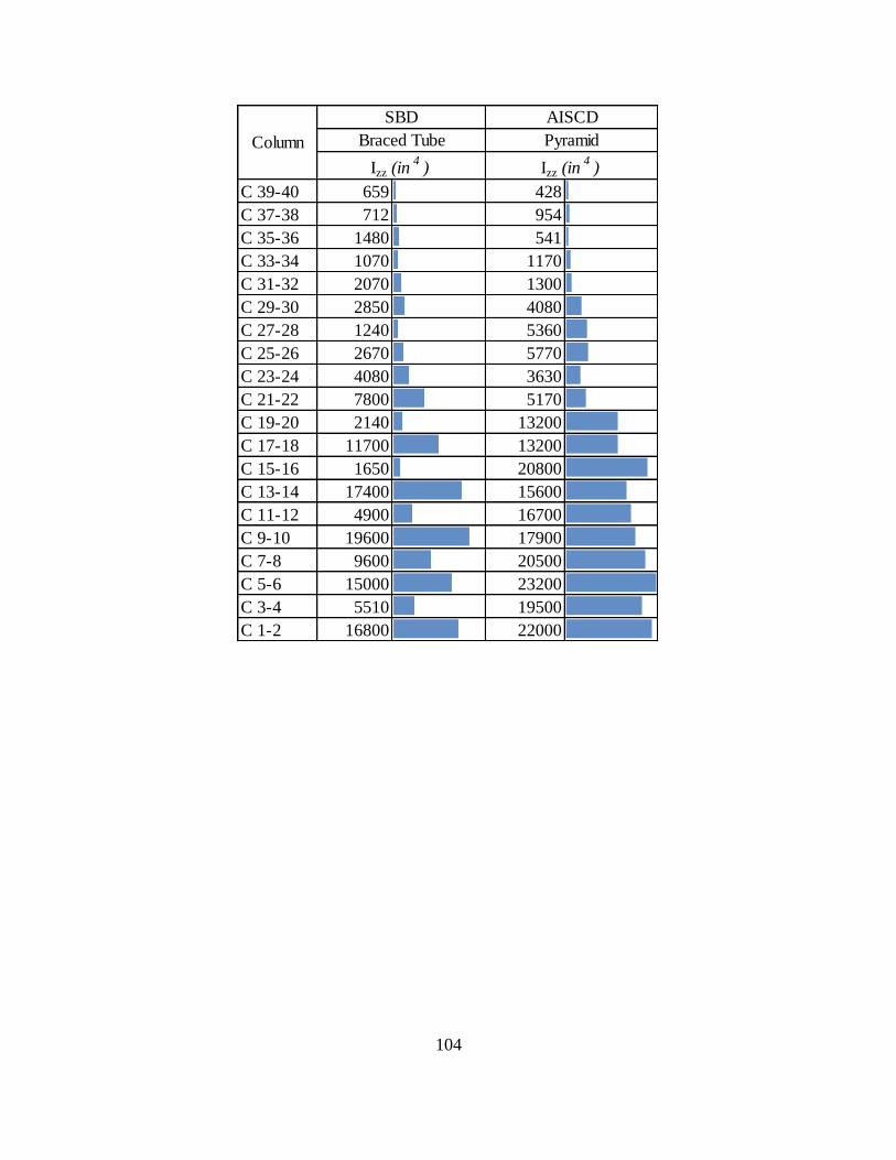
104
C 39-40 659 428
C 37-38 712 954
C 35-36 1480 541
C 33-34 1070 1170
C 31-32 2070 1300
C 29-30 2850 4080
C 27-28 1240 5360
C 25-26 2670 5770
C 23-24 4080 3630
C 21-22 7800 5170
C 19-20 2140 13200
C 17-18 11700 13200
C 15-16 1650 20800
C 13-14 17400 15600
C 11-12 4900 16700
C 9-10 19600 17900
C 7-8 9600 20500
C 5-6 15000 23200
C 3-4 5510 19500
C 1-2 16800 22000
Braced Tube PyramidColumn
SBD AISCD
Izz (in4
) Izz (in4
)

105
C 59-60 307 156
C 57-58 1070 238
C 55-56 2850 959
C 53-54 2070 890
C 51-52 1490 1110
C 49-50 2670 2070
C 47-48 1430 3000
C 45-46 5770 5900
C 43-44 16700 10500
C 41-42 11700 8160
C 39-40 15500 7020
C 37-38 13200 20800
C 35-36 10800 13200
C 33-34 16700 16700
C 31-32 19400 21900
C 29-30 19600 21900
C 27-28 16200 21900
C 25-26 13100 19500
C 23-24 4060 25600
C 21-22 29900 22000
C 19-20 28900 32000
C 17-18 16200 24300
C 15-16 14600 32000
C 13-14 6000 41600
C 11-12 24500 32100
C 9-10 16200 36000
C 7-8 6600 50400
C 5-6 6000 41600
C 3-4 32000 39600
C 1-2 36000 50600
Diagrid DiagridColumn
SBD AISCD
Izz (in4
) Izz (in4
)