Stromingsberekeningen voor het ontwerp van stoomkraakreactoren
324
Transcript of Stromingsberekeningen voor het ontwerp van stoomkraakreactoren


Stromingsberekeningen voor het ontwerp van stoomkraakreactoren
Computational Fluid Dynamics-Based Design of Steam Cracking Reactors
Carl Schietekat
Promotoren: prof. dr. ir. K. Van Geem, prof. dr. ir. G. B. MarinProefschrift ingediend tot het behalen van de graad van Doctor in de Ingenieurswetenschappen: Chemische Technologie
Vakgroep Chemische Proceskunde en Technische ChemieVoorzitter: prof. dr. ir. G. B. MarinFaculteit Ingenieurswetenschappen en ArchitectuurAcademiejaar 2014 - 2015

ISBN 978-90-8578-810-2NUR 952Wettelijk depot: D/2015/10.500/54

Stromingsberekeningen voor het ontwerp van stoomkraakreactoren Computational Fluid Dynamics-based Design of Steam Cracking Reactors
Carl Schietekat
Promotoren: prof. dr. ir. Kevin M. Van Geem en prof. dr. ir. Guy B. Marin Proefschrift ingediend tot het behalen van de graad van Doctor in de Ingenieurswetenschappen: Chemische Technologie
Vakgroep Chemische Proceskunde en Technische Chemie Voorzitter: prof. dr. ir. Guy B. Marin Faculteit Ingenieurswetenschappen en Architectuur Academiejaar 2014 – 2015

Referentie: ... ISBN-nummer: The author and the promotors give the authorization to consult and to copy parts of this work for
personal use only. Every other use is subject to the copyright laws. Permission to reproduce any
material contained in this work should be obtained from the author.

Promotoren:
prof. dr. ir. Guy B. Marin
Laboratorium voor Chemische Technologie
Vakgroep Chemische Proceskunde en Technische Chemie
Universiteit Gent
prof. dr. ir. Kevin M. Van Geem
Laboratorium voor Chemische Technologie
Vakgroep Chemische Proceskunde en Technische Chemie
Universiteit Gent
Decaan: Prof. dr. ir. Rik Van de Walle
Rector: Prof. dr. Anne De Paepe
De auteur genoot tijdens de onderzoeksactiviteiten de financiële steun van een aspirant mandaat van het Fonds voor Wetenschappelijk Onderzoek (FWO).

EXAMENCOMMISSIE
Leescommissie
Prof. dr. ir. Kevin Van Geem [promotor]
Laboratorium voor Chemische Technologie
Vakgroep Chemische proceskunde en Chemische Technologie
Faculteit Ingenieurswetenschappen en Architectuur
Universiteit Gent
Prof. dr. ir. Joris Degroote
Mechanica van Stroming, Warmte en Verbranding
Faculteit Ingenieurswetenschappen en Architectuur
Universiteit Gent
Prof. dr. ir. Rodney O. Fox
Chemical and Biological Engineering Department
College of Engineering
Iowa State University
Dr. ir. David Brown
Refining & Chemicals
Process & Project Feasibility Division
Refining & Base Chemicals Process Department
Total Research & Technology Feluy

Andere leden
Prof. dr. ir. Guy B. Marin [promotor]
Laboratorium voor Chemische Technologie
Vakgroep Chemische Proceskunde en Technische Chemie
Universiteit Gent
Prof. dr. Marie-Françoise Reyniers
Laboratorium voor Chemische Technologie
Vakgroep Chemische Proceskunde en Technische Chemie
Universiteit Gent
Prof. dr. ir. Geraldine Heynderickx
Laboratorium voor Chemische Technologie
Vakgroep Chemische Proceskunde en Technische Chemie
Universiteit Gent
Prof. dr. ir. Luc Taerwe [voorzitter]
Vakgroep Bouwkundige Constructies
Universiteit Gent

Voor mijn ouders en broer

Acknowledgements
Vooreerst wil ik mijn promotoren, prof. dr. ir. Guy B. Marin en prof. dr. ir. Kevin M. Van Geem
bedanken voor de kansen die ze me geboden hebben tijdens dit doctoraat. Ook wens ik jullie te
bedanken voor de constructieve revisies van mijn artikels en doctoraatsthesis. Zonder jullie hulp
en advies was dit werk nooit tot stand gekomen.
Many thanks go out to prof. Fox and his colleagues, prof. Alberto Passalacqua and dr. Bo Kong,
for giving me the opportunity to work 2 months at Iowa State University. Thanks for sharing your
expertise in Computational Fluid Dynamics and helping me take my first steps in OpenFOAM®.
Thanks also go out to prof. Qian for hosting me at the East China University of Science and
Technology. For the resulting fruitful collaboration on the modeling of steam cracking furnaces, I
thank dr. Hu and Yu.
During my research, I had the opportunity to participate in several collaborations with companies.
Specifically, I wish to thank dr. Marco van Goethem for the collaboration on the Swirl Flow
Tube® technology and dr. Larry Kool for the project on the YieldUp® coating. I wish you all the
best with the further development and commercialization of these technologies.
Veel dank gaat ook uit naar mijn masterproefstudenten; David Van Cauwenberghe, Pieter
Verhees en Pieter Reyniers voor hun rechtstreekse en onrechtstreekse bijdragen tot dit werk.
Sommigen hebben zich zelfs na hun masterproef nog blijvend ingezet voor dit werk, waarvoor
zeer veel dank!
Het experimentele luik van dit werk zou onmogelijk geweest zijn zonder de expertise en hulp van
Michaël Lottin, Hans Heene, Erwin Turtelboom, Bert Depuydt en Brecht Vervust. Georges
Verenghen wil ik bedanken voor het onderhouden van de servers en de hulp bij alle computer-

technische problemen. Vele berekeningen van dit werk werden uitgevoerd op de High
Performance Cluster van de Universiteit Gent. Bedankt aan het HPC team o.l.v. van dr. Ewald
Pauwels voor de uitstekende ondersteuning.
Het is aangenaam werken op een plaats waar je omringd wordt door fijne collega’s. Ik wil dan
ook de vele collega’s met wie ik gedurende deze 4,5 jaar de dag doorbracht bedanken voor de
fijne momenten, in het bijzonder diegenen met wie ik het bureau deelde; Steven, Nick, Thomas,
Ruben en recenter Pieter en Ismaël. Next, I would like to thank the TREE group colleagues and
respective girlfriends that over the last years have become a group of friends that I hold dearly:
David, Natália, Andres, Marko, Ruben DB, Pieter V, Ruben VDV, Nenad, Yu, Barbara, Silke
and Roshanak. Also many thanks go out to the other colleagues for the talks and laughs during
the coffee breaks, the weekend fun and the sunny barbeques: Gonzalo, Maria, Panos, Marita,
Daria, Pieter D, Gilles, Maarten, Kenneth, Bart, Borre, Ezgi and many, many others.
Bedankt ook aan mijn vrienden en familie voor het voorzien van de nodige afleiding in de
weekends en vakanties: Joos, Bieke, Mieke, Philippe, Stijn, Evie, Jeroen, Grazzi, Tinne, Stefaan,
Vanessa, Pieter en Thomas. Mijn broer wil ik bedanken om me 3 jaar lang te tolereren als
huisgenoot, mijn geklaag over divergerende simulaties en verstopte reactoren te aanhoren en om
me steeds te steunen. Bedankt ook om me -samen met Laure- gedurende de laatste, hectische
maanden van 2014 vaak te voorzien van een gezond avondmaal. Tenslotte wil ik mijn ouders
bedanken om me in alles te steunen en om steeds in mij te geloven.
Carl Schietekat
Gent 2015

Contents I
Contents
Notation ........................................................................................................................................ VII
Samenvatting ................................................................................................................................ XV
Summary ...................................................................................................................................... XX
Glossary .................................................................................................................................... XXIV
Chapter 1: Introduction and outline ................................................................................................. 1
1.1 Introduction ....................................................................................................................... 1
1.2 Steam cracking process ..................................................................................................... 5
1.3 Coke formation and mitigation .......................................................................................... 9
1.4 Fundamental modeling approach ..................................................................................... 13
Reaction network ...................................................................................................... 14 1.4.1
Reactor model .......................................................................................................... 16 1.4.2
1.5 Outline ............................................................................................................................. 19
References .................................................................................................................................. 22
Chapter 2: Swirl Flow Tube reactor technology: experimental and computational fluid dynamics
study ............................................................................................................................................... 29
Abstract ....................................................................................................................................... 30
2.1 Introduction ..................................................................................................................... 30

II Contents
2.2 Experimental set-up and procedure ................................................................................. 34
2.3 Numerical simulation procedure ..................................................................................... 37
Mathematical model ................................................................................................. 37 2.3.1
Grid generation ......................................................................................................... 39 2.3.2
Boundary conditions ................................................................................................ 40 2.3.3
Numerical solution ................................................................................................... 40 2.3.4
2.4 Results and discussion ..................................................................................................... 41
Experimental results ................................................................................................. 41 2.4.1
Simulation results ..................................................................................................... 45 2.4.2
2.5 Conclusions ..................................................................................................................... 55
References .................................................................................................................................. 56
Chapter 3: Computational Fluid Dynamics-based design of finned steam cracking reactors........ 59
Abstract ....................................................................................................................................... 60
3.1 Introduction ..................................................................................................................... 61
3.2 CFD model setup ............................................................................................................. 67
Governing equations ................................................................................................ 67 3.2.1
Turbulence modeling ................................................................................................ 68 3.2.2
Boundary conditions ................................................................................................ 69 3.2.3
Chemistry model ...................................................................................................... 69 3.2.4

Contents III
Numerical model ...................................................................................................... 70 3.2.5
Computational grid ................................................................................................... 71 3.2.6
3.3 CFD model validation ..................................................................................................... 72
3.4 Parametric study .............................................................................................................. 74
Fin height .................................................................................................................. 76 3.4.1
Helix angle ............................................................................................................... 79 3.4.2
Number of fins ......................................................................................................... 80 3.4.3
Geometry optimization ............................................................................................. 82 3.4.4
3.5 Reactive simulations of an industrial propane cracker .................................................... 84
Process conditions and reactor configurations ......................................................... 84 3.5.1
Results and discussion .............................................................................................. 86 3.5.2
3.6 Conclusions ................................................................................................................... 101
References ................................................................................................................................ 102
Chapter 4: Computational Fluid Dynamics simulations with detailed chemistry: Application of
Pseudo-Steady State Approximation ............................................................................................ 107
Abstract ..................................................................................................................................... 108
4.1 Introduction ................................................................................................................... 109
4.2 Numerical models .......................................................................................................... 114
Governing equations .............................................................................................. 114 4.2.1

IV Contents
Calculation rate of production term ....................................................................... 121 4.2.2
4.3 Results and discussion ................................................................................................... 127
One-dimensional vs. three-dimensional reactor model .......................................... 127 4.3.1
Validation and speedup .......................................................................................... 131 4.3.2
Simulation of an industrial propane-cracking reactor ............................................ 135 4.3.3
4.4 Conclusions ................................................................................................................... 153
References ................................................................................................................................ 155
Chapter 5: The importance of turbulence-chemistry interaction for CFD simulations ................ 161
5.1 Introduction ................................................................................................................... 162
5.2 Model equations ............................................................................................................ 164
Conservation equations .......................................................................................... 164 5.2.1
Species rate of formation ........................................................................................ 168 5.2.2
5.3 Solution procedure ......................................................................................................... 169
Conservation equations .......................................................................................... 169 5.3.1
Turbulence-chemistry interaction .......................................................................... 170 5.3.2
Dynamic zoning method ........................................................................................ 174 5.3.3
5.4 Results and discussion ................................................................................................... 176
Dynamic zoning method ........................................................................................ 176 5.4.1
Impact of turbulence-chemistry interaction ........................................................... 187 5.4.2

Contents V
Simulation of an industrial steam cracking reactor ................................................ 194 5.4.3
5.5 Conclusions ................................................................................................................... 199
References ................................................................................................................................ 201
Chapter 6: Catalytic coating for reduced coke formation ............................................................ 205
Abstract ..................................................................................................................................... 206
6.1 Introduction ................................................................................................................... 206
6.2 Experimental section ..................................................................................................... 211
Coating ................................................................................................................... 211 6.2.1
Jet stirred reactor .................................................................................................... 211 6.2.2
Experimental procedures and conditions in the jet stirred reactor ......................... 212 6.2.3
Pilot plant setup ...................................................................................................... 213 6.2.4
Experimental procedures and conditions in the pilot plant setup ........................... 215 6.2.5
6.3 Experimental results and discussion .............................................................................. 219
Jet stirred reactor .................................................................................................... 219 6.3.1
Pilot plant setup ...................................................................................................... 231 6.3.2
6.4 Simulation of an industrial ethane steam cracking unit ................................................. 235
Furnace and reactor model ..................................................................................... 235 6.4.1
Description of the industrial unit ............................................................................ 239 6.4.2
Simulation results ................................................................................................... 244 6.4.3
VI Contents
6.5 Conclusions ................................................................................................................... 249
References ................................................................................................................................ 250
Chapter 7: Conclusions and perspectives ..................................................................................... 255
7.1 Conclusions ................................................................................................................... 255
7.2 Perspectives ................................................................................................................... 258
References ................................................................................................................................ 264
Appendix A: Validation reduced kinetic models ..................................................................... 265
A.1 Propane kinetic model of Chapter 3 .............................................................................. 265
A.2 Propane kinetic model of Chapter 4 .............................................................................. 269
A.3 Butane kinetic model of Chapter 5 ................................................................................ 272
References ................................................................................................................................ 274
Appendix B: Grid independence .............................................................................................. 275
Appendix C: Averaging procedures ......................................................................................... 277

Notation VII
Notation
Roman symbols
A pre-exponential factor in (modified) Arrhenius
equation [s,mol,m³]
b temperature exponent in modified Arrhenius equation [-]
Ci- molecules with i or less carbon atoms [-]
Ci+ molecules with i or more carbon atoms [-]
�� concentration of species j [mol/m³]
�� mass specific heat capacity at constant pressure [J/kg/K]
�� molar specific heat capacity at constant pressure [J/mol/K]
d a feature representing the thermochemical state in a
grid cell [variable]
D diffusion coefficient [m²/s]
e fin height [m]
�� activation energy [J/mol/K]
surface roughness [m]
F molar flow rate [mol/s]
�� Fanning friction factor [-]
h specific enthalpy [J/mol]
Gauss-Hermite orthogonal polynomial of ith order [-]

VIII Notation
� alternative Gauss-Hermite orthonormnal polynomial
of ith order [-]
∆ reaction enthalpy of reaction i [J/mol]
I turbulence intensity [-]
� diffusional flux of species j [mol/m²/s]
�� Boltzmann constant, 1.3806 10-23 [m²/kg/s²/K]
� reaction rate coefficient of reaction i [mol/m³/s]
l turbulence length scale [m]
L length [m]
MM molecular mass [kg/mol]
N Gaussian quadrature order [-]
nreac number of reactions [-]
nspec number of species [-]
Nu Nusselt number [-]
OD maximum tube inner diameter of a finned tube, i.e.
between opposite fin valleys [m]
Pr Prandtl number [-]
q heat flux [W/m²]
Q heat [W]
r radial coordinate [m]
�� bend radius [m]
� reaction rate of reaction i [mol/m³/s]

Notation IX
�� rate of production of species j [mol/m³/s]
Re Reynolds number [-]
�� strain rate tensor [s-1]
�� any additional energy source, e.g. by radiation [W/m³]
�� heat of reaction [W/m³]
�� any additional momentum source, e.g. gravitational [kg/m²/s]
Sc Schmidt number [-]
t minimum wall thickness [m]
T temperature [K]
U global heat transfer coefficient [W/m²/K]
w fin width [m]
y distance to the wall [m]
z axial distance [m]
� specific total energy [J/kg]
���� probability density function of temperature [-]
� universal gas constant, 8.314 [J/mol/K]
� turbulent kinetic energy [m²/s²]
� pressure [Pa]
time [s]
! velocity vector [m/s]
" Gaussian quadrature weight of order i [-]
# Gaussian quadrature abscissa of order i [-]

X Notation
#� molar fraction of species j [-]
$ mass fraction of species i [-]
Greek Symbols
%� stoichiometric coefficient of species j in reaction i [-]
% correction factor on friction coefficient or Nusselt number [-]
& thermal conductivity [J/m²/s]
' density [kg/m³]
() mass flow rate [kg/s]
*+ stress tensor [Pa]
, turbulent kinetic energy dissipation rate [m²/s³]
, threshold value for the variable i [variable]
,-. Lennard-Jones well depth [m²/kg/s²]
,/ Temperature variance dissipation [K²/s]
0 Nekrasov additional resistance coefficient for bends [-]
1-. Lennard-Jones distance at which the intermolecular potential
between the two particles is zero
[m]
1/2 Temperature variance [K²]
3 azimuthal coordinate [rad]
4 viscosity [kg/m/s]

Notation XI
5 specific turbulence dissipation rate =
6
7.79: [1/s]
Ω cross-sectional area [m²]
Sub- and superscripts
< mean
+ dimensionless
avg mixing cup average
c consumption
center at the centerline
CFD raw result from CFD simulation
corr calculated from a correlation
eff effective, i.e. sum of laminar and turbulent contributions
eq equivalent
exp calculated from experimental results
ext external
f fluid mixture
h heated
i reaction i
inlet inlet
int internal, inner
j species j

XII Notation
l laminar
LJ Lennard-Jones
max maximum
outlet outlet
p production
rms root mean square
s solid
sim simulated value, after correction for tube roughness
t turbulent
T temperature
y based on the distance to the wall

Notation XIII
Acronyms
BFW Boiler Feed Water
CFL Courant-Friedrichs-Lewy number
CIP Coil Inlet Pressure, i.e. the process gas pressure at the inlet of the reactor, just
upstream the radiation section, just downstream the critical venturi nozzle
COP Coil Outlet Pressure, i.e. the process gas pressure at the outlet of the reactor, just
upstream the adiabatic volume
COT Coil Outlet Temperature, i.e. the process gas temperature at the outlet of the
reactor, just upstream the adiabatic volume
CPU Central processing unit, i.e. the electronic circuitry that carries out the
instructions of a computer program by performing the basic arithmetic, logical,
control and input/output (I/O) operations.
CSP Computational Singular Perturbation
CSTR Continuously Stirred Tank Reactor
DMDS DiMethyl DiSulfide
DNS Direct Numerical Simulation
DRG Directed Relation Graph
DS Dilution Steam
EOR End-Of-Run
ILDM Intrinsic Lower Dimensional Manifold
LES Large Eddy Simulation

XIV Notation
LMTD Log Mean Temperature Difference
LPG Liquefied Petroleum Gas
P/E Propene-to-Ethene ratio, a cracking severity index
PAH PolyAromatic Hydrocarbons
PE Partial Equilibrium
PFO Pyrolysis Fuel Oil
PGC Process Gas Compressor
PSS Pseudo-Steady State
PSSA Pseudo-Steady State Assumption
pygas pyrolysis gasoline
QUICK Quadratic Upstream Interpolation for Convective Kinematics
SIMPLE Semi-Implicit Method for Pressure-Linked Equations
SOR Start-Of-Run
SST Shear-Stress Transport
TLE Transfer-Line Exchanger, i.e. the heat exchanger of a steam cracking furnace
downstream the adiabatic volume
TMT external skin Tube Metal Temperature
tpy metric tons per year, i.e. 1000 kg per year

Samenvatting XV
Samenvatting
Stoomkraken van koolwaterstoffen is een petrochemisch proces dat een groot deel van de
basischemicaliën van de chemische industrie produceert, met name olefinen en aromaten.
Conventionele voedingen voor het proces zijn derivaten van aardgas en aardolie zoals lichte
gassen (ethaan, propaan, butaan), nafta’s en gasolies. Deze voedingen worden verwarmd tot 820-
890 °C in tubulaire reactoren die in grote ovens hangen. Deze hoge temperaturen initiëren de
thermochemische omzetting naar de producten van het proces, namelijk olefinen (etheen en
propeen) en aromaten (benzeen, tolueen, xyleen en styreen) en verschillende bijproducten. De
huidige globale productiecapaciteit is meer dan 150 miljoen ton etheen per jaar. Verwachtingen
zijn dat deze over de komende jaren zal stijgen, gedreven door nieuwe installaties en
uitbreidingen in China, het Midden-Oosten en de Verenigde Staten.
Ongewenste reacties zorgen voor de vorming van een cokeslaag op de binnenwand van de reactor.
Deze groeiende cokeslaag heeft twee negatieve gevolgen. Ten eerste, stijgt de drukval over de
reactor waardoor de selectiviteit naar het belangrijkste product etheen daalt. Ten tweede, stijgt de
temperatuur van het reactormateriaal gedurende de afzetting van de cokeslaag doordat cokes
sterk isolerende eigenschappen heeft. Wanneer de drukval over de reactor of de temperatuur van
het reactormateriaal vooraf gedefinieerde waarden overstijgt, wordt de oven uit dienst genomen
om de cokeslaag van de reactoren af te branden met een lucht/stoom mengsel. De duur van één
zo’n productiecyclus wordt de runlengte van de oven genoemd en is uiteraard sterk afhankelijk
van de procescondities zoals temperatuur en voeding. De cyclische operatie tussen kraken en
ontkolen van de ovens heeft een negatieve invloed op de beschikbaarheid en rendabiliteit van
kraakeenheden. Om deze reden, hebben vele onderzoeksprogramma’s geleid tot de ontwikkeling
XVI Samenvatting
van een uitgebreid gamma aan technologieën om de vorming van cokes te reduceren. Twee
technologieën werden in dit werk onderzocht, namelijk driedimensionale reactorgeometrieën en
een katalytische coating.
Bij de driedimensionale reactorgeometrieën, wordt de geometrie van de binnenwand van de
reactor aangepast om een hogere convectieve warmteoverdracht te verkrijgen en/of om de
warmte uitwisselende oppervlakte te vergroten. Door de betere warmteoverdracht, is de
temperatuur van het reactormateriaal lager en is de runlengte langer. De aanpassingen van de
reactorgeometrie zorgen echter voor een verhoogde drukval die de selectiviteit naar de gewenste
producten beïnvloedt. Kwantificatie van dit effect aan de hand van industriële of pilootplant
resultaten is om verschillende redenen onnauwkeurig. Daarom was het hoofddoel van dit werk de
ontwikkeling en toepassing van numerieke simulatiecodes om het effect van deze
driedimensionale reactortechnologieën op product selectiviteiten en cokesvormingssnelheid te
kwantificeren.
In hoofdstuk 2, wordt een recent ontwikkelde driedimensionale reactor technologie genaamd
Swirl Flow Tube® onderzocht op basis van experimenten en simulaties. De dwarsdoorsnede van
een Swirl Flow Tube® is nog steeds schijfvormig zoals deze van een conventionele rechte
reactorbuis, maar de middellijn volgt een helicoïdaal pad in plaats van een rechte lijn om een
betere menging te verkrijgen. De experimentele resultaten tonen aan dat de globale
warmteoverdrachtscoëfficiënt 1.2 tot 1.5 keer hoger is in vergelijking met een rechte buis. De
ongewenste drukval is beperkt tot 1.4 tot 2.2 keer die van een rechte buis. Een numeriek
stromingsmodel werd gebruikt om de experimenten te simuleren en toonde een goede
overeenkomst met de experimentele resultaten. Het model geeft aan dat de verhoogde

Samenvatting XVII
warmteoverdracht en drukval te verklaren zijn door een hogere schuifspanning. De resultaten
bevestigen het potentieel van de applicatie van de SFT® technologie in stoomkraakreactoren.
De kwantificatie van het effect van de verhoogde warmteoverdracht en drukval op product
opbrengsten en cokesvorming vereist het implementeren van een gasfase reactie model en een
cokesmodel in het stromingsmodel. In hoofdstuk 3 worden dergelijke driedimensionale
stromingssimulaties besproken voor de evaluatie van gevinde reactorbuizen. Het wordt
aangetoond dat voor een bepaald industrieel reactorontwerp de maximale temperatuur van het
reactormateriaal met 50 K verlaagd kan worden wanneer optimale geometrische parameters voor
de vinnen gebruikt worden. Hierdoor daalt de cokesvormingssnelheid met 50 %. De drukval
over de reactor stijgt echter met ongeveer 50 % en resulteert in kleine, maar significante
veranderingen in de selectiviteiten van de lichte olefinen.
Het gebruik van gedetailleerde chemie in stromingssimulaties geeft aanleiding tot zeer lange
simulatietijden. Daarom werd in hoofdstuk 4 een methode ontwikkeld om gedetailleerde,
fundamentele reactiemodellen te gebruiken in stromingssimulaties door toepassing van de
pseudo-stationaire toestandshypothese (PSSH). Naargelang de grootte van het reactiemodel, werd
een reductie van de simulatietijd met een factor van 7 tot 54 verkregen. Een industriële reactor
werd gesimuleerd voor zowel een standaard, rechte buis als voor een geoptimaliseerde gevinde
buis. Vergelijking van de resultaten van het 3D model met een meer gebruikelijk 1D reactor
model toonde aan dat een significante fout gemaakt wordt in het 1D model door de verhoogde
reactiesnelheden in de laminaire film aan de binnenwand van de reactor te verwaarlozen. Daarom
werd het 1D model uitgebreid om rekening te houden met deze laminaire film.
Het hierboven vermelde onderzoek werd uitgevoerd met behulp van het commerciële programma
FLUENT®. Aangezien er geen toegang tot de broncode van dit programma beschikbaar is, zijn de

XVIII Samenvatting
mogelijkheden van de gebruiker om de code aan te passen naar de specifieke noden van het
beschouwde probleem beperkt. Verder, is parallellisatie van de simulaties over vele honderden
CPU’s moeilijk doordat per CPU een licentie nodig is. Daarom werd in hoofdstuk 5 een code
ontwikkeld voor de driedimensionale simulatie van stoomkraakreactoren op basis van het gratis,
open source pakket OpenFOAM®. Het effect van turbulente temperatuurschommelingen op de
reactiesnelheden werd gekwantificeerd door het gebruik van een waarschijnlijkheidsdichtheid
voor de temperatuur. Het effect of de opbrengst van de verschillende producten is bij
gebruikelijke procescondities beperkt tot 0.1 wt%. Om de simulatietijd verder te beperken, werd
een dynamische zoningsmethode geïmplementeerd. Tenslotte, werd de code succesvol
aangewend voor de simulatie van een industriële reactor voor het kraken van butaan.
Zoals eerder vermeld, werd naast driedimensionale reactoren, ook een katalytische coating
bestudeerd. Bij deze technologie wordt een katalysator als een coating op de binnenwand van de
reactor aangebracht. Deze katalysator zet cokes om tot koolstofoxides en waterstof door reactie
met de verdunningsstoom tijdens het kraken van de voeding. Op deze manier wordt minder cokes
afgezet in de reactor en wordt de runlengte verlengd. In hoofstuk 6, werd een dergelijke
katalytische coating, genaamd YieldUp® experimenteel getest en werd de opschaling naar een
industriële eenheid gemaakt met numerieke simulaties. Drie verschillende formulaties van de
coating werden getest in een jet-geroerde reactor en vertoonden alle een verlaagde
cokesvormingssnelheid over meerdere kraken/ontkolen cycli in vergelijking met een referentie
reactormateriaal. De meest performante formulatie werd verder getest in een pilootplant. De
totale cokesvorming werd met 76 % verminderd door toepassing van de coating. Opschaling van
de coating naar een industriële ethaankraker werd gesimuleerd met gekoppelde oven-reactor
simulaties. Toepassing van de coating resulteerde in een verlenging van de runlengte met meer

Samenvatting XIX
dan 400 % en een verhoging van de ongewenste CO en CO2 opbrengsten tot 216 ppmw en 344
ppmw. Deze relatief hoge CO2 opbrengst is een potentieel probleem voor de downstream
eenheden.

XX Summary
Summary
Steam cracking of hydrocarbons is a petrochemical process that provides the bulk share of base
chemicals for the chemical industry, i.e. olefins and aromatics. The hydrocarboneous feedstocks
conventionally used in the process, originate from natural gas and crude oil and range from light
gasses such as ethane, propane and butane to liquids such as naphthas and gas oils. These
feedstocks are heated to 820-890 °C in tubular reactors suspended in large fired furnaces. These
high temperatures initiate the thermochemical conversion to the process products, i.e. olefins
(mainly ethene and propene) and aromatics (mainly benzene, toluene, xylenes and styrene).
Current global production capacity of ethene is over 150 million metric tons per year and is
projected to grow over the next years with main additions in China, the Middle East and the
United States.
Undesired side reactions result in the formation of a coke layer on the reactor tube inner wall.
This growing layer has two negative effects. Firstly, the reactor pressure drop increases which
results in a loss of selectivity to ethene, the process’ main product. Secondly, as coke is highly
insulating, the reactor tube metal temperature increases over time during the growth of the coke
layer. When the reactor pressure drop or the tube metal temperatures are higher than predefined
maximum values, the furnace is take out of service and the coke layer is burned off using an
air/steam mixture. The duration of one cracking cycle is referred to as the furnace run length.
This cyclic operation of cracking/decoking of the furnaces has a negative influence on the cracker
economics. Therefore, many research efforts have led to the development of technologies to
mitigate the formation of coke. The two technologies investigated in this work, are three-
dimensional reactor technologies and a catalytic coating.

Summary XXI
In three-dimensional reactor technologies, the reactor tube inner geometry is altered from the
conventional bare, straight tube to a more complex geometry to enhance convective heat transfer
and/or increase heat transfer area. By the increased heat transfer, the tube metal temperature is
lowered and the run length is increased. As these geometrical modifications result in an increased
pressure drop compared to conventional bare tubes, the selectivity towards light olefins is
affected. It is difficult to quantify the selectivity effect experimentally in an industrial or pilot
plant. Hence, the main goal of this work was to develop and use numerical simulation tools to
quantify the impact of three dimensional reactor technologies on product selectivities and coking
rate.
In Chapter 2, a recently developed three-dimensional reactor technology called Swirl Flow Tube®
(SFT®) is evaluated experimentally and numerically. The cross section of the SFT® remains
circular like a conventional, straight tube but the centerline follows a helicoidal path providing
enhanced mixing. The experimental results show that the heat transfer coefficient increases with
a factor of 1.2 to 1.5 compared to a straight tube. The undesired pressure drop increase factor is
only 1.4 to 2.2 which is moderate compared to other technologies. A computational fluid
dynamic (CFD) model was adopted that showed satisfactory agreement to the experimental
results. The increased heat transfer and pressure drop can be attributed to a higher wall shear
stress. The results show the potential for the application of the SFT® technology in steam
cracking reactor designs.
The effect of the increased heat transfer and pressure drop on product yields and coke formation
can be accounted for by implementing a gas-phase reaction model and a coking model. In
Chapter 3, such three-dimensional CFD simulations are discussed for the evaluation of finned
reactor tubes. It was shown that the reactor tube metal temperatures can be reduced by up to 50 K
XXII Summary
when applying optimal fin parameters compared to the equivalent bare tubes and that coking
rates are reduced by up to 50 %. However, the increased friction and inner surface area lead to a
pressure drop increase of about 50 % which causes small but significant shifts in light olefin
selectivity.
Implementation of detailed chemistry in computational fluid dynamics results in very high
simulation times. Therefore, in Chapter 4 a methodology is developed to use detailed single-event
microkinetic reaction networks by on the fly application of the pseudo-steady state assumption
(PSSA). Depending on the reaction network size, a speedup factor from 7 to 54 was obtained
compared to standard routines. An industrial propane cracking reactor was simulated using both a
conventional bare reactor and a helicoidally finned reactor. Comparison of the simulation results
using the developed 3D model and a more conventionally used 1D reactor model shows that a
significant error is made by neglecting the increased reaction rates in the laminar film near the
reactor inner wall. Therefore the 1D plug flow reactor model was extended to account for the
non-uniform radial temperature profile which resulted in a closer agreement between the 1D and
3D model.
All previously discussed work was performed using the commercial CFD package FLUENT®. As
there is no access to the source code, the possibilities to adjust the code to the specific needs of
simulating a steam cracking reactor are limited. Furthermore, massive parallelization of a
simulation over hundreds or thousands of CPU’s is very expensive because of license limitations.
Hence, in Chapter 5, a code was developed for the three-dimensional simulation of steam
cracking reactors based on the free, open source CFD software package OpenFOAM®. The effect
of turbulent temperature fluctuations on the reaction rates was quantified by a probability density
function for temperature. The effect on product yields under typical steam cracking conditions

Summary XXIII
was seen to be limited to about 0.1 wt%. To further reduce the computational time, a dynamic
zoning method was implemented besides the application of PSSA. Finally, the code was
successfully applied for the simulation of an industrial butane cracking reactor.
As mentioned previously, a catalytic coating to reduce coke formation was also studied in this
work. This technology comprises the coating of the reactor inner wall with a catalyst that
converts coke to carbon oxides and hydrogen by reaction with the dilution steam. In Chapter 6, a
catalytic coating called YieldUp® was tested experimentally and the scale up to an industrial unit
was simulated. Three different formulations of the coating were tested in a jet-stirred reactor
setup and showed reduced coking rates over multiple coking/decoking cycles compared to a
reference alloy. The best coating was further tested in a pilot plant. The overall coke formation
was reduced by 76 % compared to a reference alloy reactor. Scale-up was assessed by simulating
an industrial ethane cracking reactor. Application of the coating resulted in a simulated increase
of the reactor runlength by a factor of five while the CO and CO2 yields were limited to 216
ppmw and 344 ppmw respectively. This relatively high CO2 yield can be higher than the
specifications of downstream units depending on the design of the caustic tower.

XXIV Glossary
Glossary
µ-radical A radical for which bimolecular reactions can be neglected.
µ-radical hypothesis The hypothesis that radicals with more than 5 carbon atoms are
µ-radicals
3D reactor technology A reactor technology that enhances heat transfer by geometrical
modifications to the traditional straight, bare tube used as tubular
reactors.
Ab initio Latin term for “from first principles”. It refers to the fact that the
results are obtained by applying the established laws of nature
without assumptions, special models or experimental input. Ab
initio methods determine the energy of a molecule or transition
state by solving the Schrödinger equation.
Arrhenius activation energy The coefficient Ea describing the temperature dependency of the
rate coefficient k = A exp (−Ea/RT) with A the temperature
independent pre-exponential factor.
Arrhenius pre-exponential factor
See Arrhenius activation energy.
Catalytic coking mechanism Mechanism that explains the formation of coke by action of a
catalyst (typically Fe or Ni) during steam cracking processes.
COILSIM1D Fundamental model for the simulation of steam cracking units
developed at the Laboratory for Chemical Technology of Ghent
University.

Glossary XXV
Coke Solid carbonaceous residue that deposits inside the reactor and
downstream equipment.
Computational fluid dynamics A branch of fluid mechanics that uses numerical methods and
algorithms to solve and analyze problems that involve fluid
flows.
Condensation coking mechanism
Mechanism that explains the formation of coke when heavy
polynuclear aromatics condense either directly on the wall or in
the bulk gas phase and subsequently collect on the wall.
CRACKSIM Single-event microkinetic model developed at the Laboratory for
Chemical Technology describing the gas-phase reactions during
steam cracking of hydrocarbons.
Energy dispersive X-ray analysis
Analytical technique that determines the elemental chemical
composition of a sample by aiming a beam of high energy
electrons to it and then quantifying the X-ray spectra emitted by
the sample.
Enthalpy The enthalpy H is a thermodynamic quantity and is calculated
from the internal energy U as H = U + pV, with p the pressure
and V the volume of the system
Entropy The entropy S is a thermodynamic property that is related to the
disorder of the system. A system with a larger number of states
that can be occupied, will therefore have a higher entropy.
Feedstock reconstruction Deriving the detailed composition of a complex feedstock (or in

XXVI Glossary
fact any other mixture) from limited macroscopic information.
Gas phase heterogeneous coking mechanism
Mechanism that explains the formation of coke due to the
interaction of precursors in the gas phase with active sites in the
surface of previously deposited coke.
Gas phase homogeneous coking mechanism
See condensation coking mechanism.
Group additivity method Technique that allows to predict properties from molecular
structures. For example, within Benson’s group additivity method
a property can be written as a sum of contributions arising from
its constituent groups.
Jet stirred reactor Type of ideal continuously stirred tank reactor where ideal
mixing is achieved by introduction of the feedstock to the reactor
via jets.
Lumping Grouping of species which are generally isomers or homologous
species with similar reactivity in order to reduce the total number
of species in a kinetic model.
one-dimensional reactor simulation
A reactor simulation using a model with one independent
variable, e.g. a batch reactor or a plug flow reactor (PFR) model.
Pseudo-steady state approximation
An approximation made that the rate of production and
consumption of a species are equal. Can be applied to multiple
species in a reaction mechanism.
Pyrolysis The uncatalyzed decomposition of organic components resulting
from exposure to high temperature, in the absence of molecular

Glossary XXVII
oxygen.
Radical coking mechanism See gas phase heterogeneous coking mechanism.
Reaction family A class of reactions that are characterized by the same pattern of
electron rearrangement steps.
Reaction path degeneracy The number of energetically equivalent paths that reactants can
follow to be converted into products.
Run length Time of operation between two decoke operations.
Scanning electron microscope Type of electron microscope that produces images of a sample by
scanning it with a focused beam of electrons.
Shale gas Natural gas trapped in shale formations.
Single-event microkinetic model
A kinetic model that consists of elementary reactions and
accounts for all energetically equivalent reaction paths, i.e.
single-events, to determine each reaction rate.
Single-event pre-exponential factor
The pre-exponential factor excluding the number of single-events
of the reaction.
Steam cracking A petrochemical process in which saturated hydrocarbons are
converted into small unsaturated hydrocarbons by exposure to
high temperature in the presence of steam.
Swirl flow A whirling or eddying flow of fluid.
Turbulence model A model to predict the effects of turbulence. The continuity
equations are often simplified by averaging, but models are
needed to represent the scales of the flow that are not resolved.

XXVIII Glossary
Wall shear stress Component of stress coplanar with the wall. It is the product of
the viscosity and the derivative of axial speed to radial
coordinate.
zero-dimensional reactor simulation
A reactor simulation using a model without any independent
variable, e.g. a continuously stirred tank reactor (CSTR) model.
β-radical A radical that undergoes both mono- and bimolecular reactions.
Chapter 1: Introduction and outline 1
Chapter 1: Introduction and outline
1.1 Introduction Global energy consumption has dramatically increased over the last 15 years with China being
the main culprit as shown in Figure 1-1. The energy demand is projected to grow by 37% to
2040, an average annual growth rate of 1.1% per year. The slowdown in growth compared to
previous decades is mainly due to energy efficiency gains and governmental changes in favor of
less energy-intensive activities. China will still have the largest share in the energy demand
growth until mid-2020’s, when its population levels off and its economic growth will slow down.
At that time, India, Southeast Asia, the Middle East and parts of Africa and Latin America are
projected to take over as the leading regions for energy demand [1]. Crude oil, natural gas and
coal are currently the main resources for energy with oil providing about 33 % of the world’s
energy usage.
The world oil supply will increase by 14 million barrels/day to 104 million barrels/day in 2040 as
shown in Figure 1-2. While oil production in the United States, Brazil, Canada and the Middle
East will grow, the rest of the world will face a net reduction in oil production. Indeed, by mid-
2020, the non-OPEC oil supply will start to fall back and the world reliance on major resource-
holding countries in the Middle East will increase [1]. Crude oil is mostly used for transportation
purposes with gasoline, diesel and jet fuel making up more than three-quarters of current oil
usage. Only about 10% of global oil production is used for the production of chemicals. The main

2 Chapter 1: Introduction and outline
petroleum cuts used for chemicals production are petroleum gasses and naphtha, a petroleum cut
with a boiling range between 300 and 470 K.
Figure 1-1: Global energy demand [GWh] as a function of time: - China; - -OECD; - Rest
of world [1].
Figure 1-2: Cumulative oil production growth [mb/day] as a function of time: - United States; -
Canada; - Brazil; - Middle East; - Other producers [1].

Chapter 1: Introduction and outline 3
All major regions, except Europe, will contribute to a more than 50% rise in natural gas output to
2040 [1]. Currently the third largest energy contributor, natural gas, will be the world’s fastest
growing major energy source through 2040 and is expected to surpass coal as second most
important energy source. The share of unconventional gas will increase from 17% to 31% in the
total natural gas output. Purified natural gas is mainly used for electricity production, residential
heating and as an industrial fuel. Natural gas liquids, e.g. ethane, propane and butanes, and gas
condensates obtained during natural gas treatment, are often used for the production of base
chemicals. With the rise of new technologies such as hydraulic fracking, the production of natural
gas trapped in shale formations, i.e. shale gas, has boomed over recent years. As shale gas can
contain more than 20 mol% of C2+ molecules, it is expected to increase natural gas liquids
production by more than 40 % [2].
Although the fraction of natural gas and oil consumption used for the production of chemicals
and materials is relatively small compared to the fraction used for transportation, heating and
electricity production, the economic importance is significant due to the higher added value of
chemicals compared to fuels and electricity. Most of these high-value chemicals and materials are
derived from a limited number of base chemicals. These main base chemicals comprise
hydrogen, olefins such as ethene, propene and 1,3-butadiene, and aromatics such as benzene,
toluene and xylenes, supplemented with some heteroatom-containing chemicals such as
ammonia, chlorine and sulfuric acid. The bulk of the olefins production and a large part of the
aromatics production proceeds through the steam cracking process with ethene being the main
product of the process. Ethene is the raw material used in the manufacture of poly(ethene),
oxirane, 1,2-dichloroethane, poly(ethene terephthalate), poly(1-chloroethene) and polystyrene as
well as fibers and other organic chemicals. Figure 1-3A shows the global ethene production,
4 Chapter 1: Introduction and outline
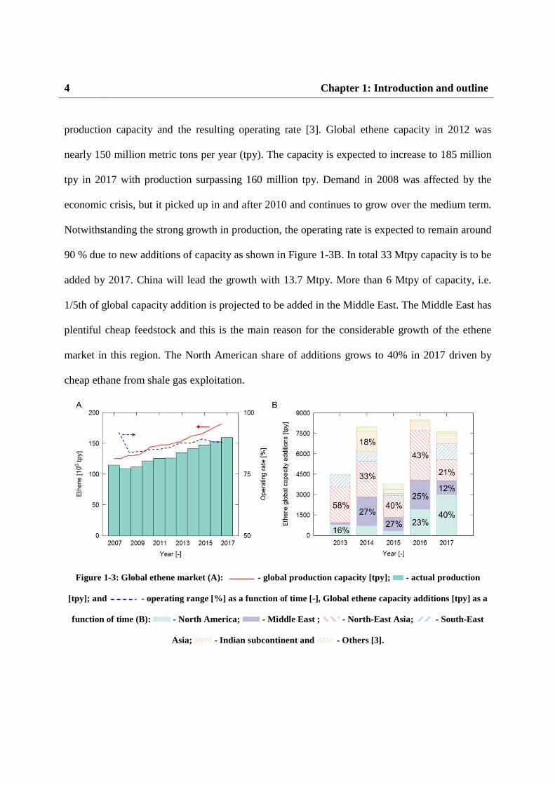
production capacity and the resulting operating rate [3]. Global ethene capacity in 2012 was
nearly 150 million metric tons per year (tpy). The capacity is expected to increase to 185 million
tpy in 2017 with production surpassing 160 million tpy. Demand in 2008 was affected by the
economic crisis, but it picked up in and after 2010 and continues to grow over the medium term.
Notwithstanding the strong growth in production, the operating rate is expected to remain around
90 % due to new additions of capacity as shown in Figure 1-3B. In total 33 Mtpy capacity is to be
added by 2017. China will lead the growth with 13.7 Mtpy. More than 6 Mtpy of capacity, i.e.
1/5th of global capacity addition is projected to be added in the Middle East. The Middle East has
plentiful cheap feedstock and this is the main reason for the considerable growth of the ethene
market in this region. The North American share of additions grows to 40% in 2017 driven by
cheap ethane from shale gas exploitation.
Figure 1-3: Global ethene market (A): - global production capacity [tpy]; - actual production
[tpy]; and - operating range [%] as a function of time [-], Global ethene capacity additions [tpy] as a
function of time (B): - North America; - Middle East ; - North-East Asia; - South-East
Asia; - Indian subcontinent and - Others [3].

Chapter 1: Introduction and outline 5
1.2 Steam cracking process A wide variety of feedstocks is used in the steam cracking process, ranging from light gasses
such as ethane, propane and butane, to liquids such as naphtha’s, gas oils, vacuum gas oils and
recently even crude oils [4]. A steam cracking unit can be roughly divided into a hot and a cold
section [5]. The most important units of the hot section are the cracking furnaces with a
convection section and a radiation section as depicted in Figure 1-4. The convection section
contains several heat exchanger banks where the feedstock and dilution steam are vaporized
and/or heated using the flue gas of the furnace. Furthermore, extra high pressure superheated
steam is produced from boiler feed water (BFW) using the hot flue gas. In the radiation section
the hydrocarbons are heated rapidly and cracked in tubular reactors. Several reactors are
suspended in a single furnace. The flow rate is uniformly distributed over the reactors via
venturi’s in the choked flow regime. Typical reactor lengths and diameters vary from 10 to 100 m
and 30 to 150 mm respectively. Reactor designs range from single-tube, short length, small
diameter reactors with many in one furnace, such as the Millisecond reactor designs; to longer,
larger diameter reactors. Longer reactors consist of multiple straight tubes connected with return
bends, often with the tubes swaged to larger diameters towards the end of the reactor. Split coils
are also popular where multiple, parallel tubes in the first passes of the reactor combine to larger
diameter outlet tubes. The heat is supplied by burners positioned in the furnace floor and/or
sidewalls. Typical coil-outlet-temperatures (COT) range from 750-890 °C depending on the
feedstock, the reactor design and the desired cracking severity. Given the high temperatures, the
reactors are made out of heat-resistant, high-Cr-Ni-alloy steels. Downstream the reactors, the
effluent is generally quenched in two steps in order to avoid subsequent reactions of the products:

6 Chapter 1: Introduction and outline
a first indirect quench with boiling water in the so-called transfer line heat exchanger(s) (TLE)
generates high pressure steam and a second direct quench with quench oil separates the heavy
from the light part of the effluent. The light hydrocarbons are compressed and the heavy
hydrocarbons are sent to a distillation column more downstream in the process. After
compression and drying, the light hydrocarbons are sent to a series of fractionators and reactors
that purify the light gases into the various plant products. Typically the following products are
obtained; fuel gas, i.e. hydrogen and methane, ethene, propene, a C4-cut with high 1,3-butadiene
content, mixed C5’s, pyrolysis gasoline (pygas) rich in aromatics, and pyrolysis fuel oil (PFO).
Ethane and propane can be recycled for cracking in a dedicated recycle furnace or used as fuels.
Depending on the feedstock and the integration with other petrochemical units, the C4-cut can be
further refined for butadiene, n-butenes, isobutene or mixtures thereof. Otherwise the C4-cut is
hydrogenated and recycled for cracking or sold directly. The pygas can be refined for aromatics
and/or hydrotreated and sent to the gasoline pool.

Chapter 1: Introduction and outline 7
Figure 1-4: Schematic drawing of a cracking furnace.
The main factors that determine the product spectrum are the feedstock, the cracking severity,
residence time, steam to oil ratio (dilution) and pressure. The heavier the feedstock and the higher
its aromatics content, the lower the ethene yield. Hence, ethane has the highest ultimate ethene
yield of all feeds, i.e. around 82 wt% at 65 % ethane once-through conversion. The cracking
severity is quantified by the conversion for light feedstocks like ethane, propane and butane and
by the propene-over-ethene ratio (P/E) for naphtha and heavier feedstocks cracking. For ethane
cracking, lower conversion results in higher ethene selectivity. However, an operational limit is
set by the flow rate in the ethane recycle, resulting in typical ethane conversions of 60-70 %. For

8 Chapter 1: Introduction and outline
naphtha cracking, the ethene yield increases with increasing severity at relevant process
conditions. An economical limit is set here by the decreasing propene yield at higher severity
resulting in typical P/E-values between 0.40 and 0.65. Plehiers and Froment [6] showed that
lower residence times require higher temperatures to obtain the desired cracking severity. At
these high temperatures, high-activation energy reactions, such as C-C and C-H β-scissions are
favored, resulting in high light olefins selectivity and low aromatics selectivity. Selectivity to
light olefins is favored by low hydrocarbon partial pressure as olefins-forming reactions are often
monomolecular while olefins-consuming reactions are mostly bimolecular. Therefore the reactor
pressure should be minimized and steam dilution maximized. A lower limit of the coil-outlet-
pressure (COP) is set by the suction pressure of the downstream process gas compressor (PGC)
which is above atmospheric pressure. The operating point of the compressor and the pressure
drop from the reactor outlet to the compressor results in typical COP’s of 0.15-0.23 MPa abs. For
the steam dilution a balance needs to be found between better ethene selectivity at high dilution
and lower energy consumption at lower dilution. Furthermore, a lower limit on steam dilution is
set by coke formation as further discussed in section 1.3 and by vaporization of the hydrocarbons
in the convection section in the case of heavy feed cracking. Indeed part of the vaporization of
the feedstock is accomplished by mixing the hot dilution steam with the partly vaporized
feedstock. These considerations have resulted in typical steam dilutions of 0.25-0.4 for ethane
and 0.35-0.60 for naphthas.

Chapter 1: Introduction and outline 9
1.3 Coke formation and mitigation Since the 1930’s it is well known that the cracking of hydrocarbons at elevated temperature,
proceeds mainly through a radical reaction mechanism [7, 8]. These gas-phase cracking reactions
are accompanied by the formation of a carbonaceous layer on the reactor inner wall [9]. This so-
called coke layer exhibits a number of negative effects on the steam cracking process’ economics
[10]. Firstly, the growing coke layer reduces the cross-sectional flow area of the reactor resulting
in higher pressure drop over time. As stated previously, a higher pressure has a detrimental effect
on the selectivity to ethene. Furthermore, coke is highly insulating and adds a growing extra
conductive resistance to the heat transfer from the furnace to the process gas. To maintain the
cracking severity, the fuel flow rate to the furnace burners is increased over time. Consequently,
the external tube metal temperature (TMT) increases over time. When the TMT reaches the
maximum allowable value or when the venturi pressure ratio (VPR) reaches a maximum
permitted value (typically 0.9), production is halted, the furnace is taken off-line and the coke
layer is burned off the reactors’ inner walls using a steam-air mixture. After ca. 20 h the decoking
of the reactors is finished and the TLEs can be decoked. Total decoking time of both reactors and
TLEs typically requires 36 h [5]. Obviously, these periodic production interruptions have a
negative effect on the process economics. Furthermore, the reactor material deteriorates with
successive coking-decoking cycles by tube corrosion, carburization and erosion [11-14].
Therefore the reactor coils need to be replaced every 4 to 10 years. Given the negative impact of
coking on the process economics, a fundamental understanding of coke formation and the
dependency of coke formation on process conditions is important for plant design and
optimization. The coke deposited in steam cracking reactors is formed via three different

10 Chapter 1: Introduction and outline
mechanisms: the catalytic, the heterogeneous non-catalytic and the homogeneous non-catalytic
coke formation mechanism.
When the gas-phase hydrocarbons are in direct contact with the reactor alloy, coke is formed
through a catalytic mechanism with the alloy providing catalytic active sites [15-18]. Evidently,
the reactor surface composition greatly influences the rate of coke formation during this catalytic
coke formation [14, 19]. Typical alloy elements that catalyze coke formation are nickel and iron,
while copper has a very low catalytic activity towards coke formation [20, 21]. In this
mechanism, a hydrocarbon molecule chemisorbs on the active site and dehydrogenates to form -
CH3, -CH2 and -CH groups on the surface together with gas-phase hydrogen [17]. The carbon
atoms left on the metal site dissolve in and diffuse through the metal particle. When the carbon
atoms exert a pressure on the metal particle higher than the tensile strength of the metal, the
particle gets lifted from the surface and carbon precipitates at the rear end of the particle. As
more carbon atoms dissolve, diffuse and precipitate, a carbon stem, so-called whisker or filament,
is formed with the metal particle at the top. During precipitation, structural deficiencies can occur
in the whiskers on which gas-phase radicals and molecules can react. This results in lateral
growth of the whiskers and interweaving of whiskers. Finally, the metal particle at the tip of the
whisker is encapsulated by coke stopping further catalytic growth of the filament.
Whereas catalytic coke formation decreases over time due to encapsulation of the active sites, the
heterogeneous, non-catalytic mechanism proceeds throughout the entire run of the reactors. As
such, the run length of industrial reactors is mainly determined by heterogeneous, non-catalytic
coke formation [22]. In this mechanism, gas-phase species react with the coke layer itself through
a radical mechanism. Wauters and Marin [10] suggested that the mechanism can be reduced to
five families of reversible elementary reactions: hydrogen abstraction from the coke layer by a

Chapter 1: Introduction and outline 11
gas-phase radical, substitution reaction of a gas-phase radical on the coke layer, radical addition
of a gas-phase radical to a surface olefinic bond, addition of a gas-phase olefinic bond to a
surface radical and cyclization of a surface radical. In theory all gas-phase radicals and molecules
can react with the coke layer, but given their respective reactivity caused by their reactive groups
and their concentration, a limited number of components, i.e. the coke precursors, dictate coke
formation.
In the third mechanism, i.e. the homogeneous, non-catalytic coke formation, small droplets
prevalent in the process gas impinge on the reactor inner wall. These droplets can rebound, splash
or stick [23]. The droplets consist of polyaromatic hydrocarbons (PAH) either present in the feed
or formed through secondary condensation reactions [24]. The PAHs form tar droplets in the gas
phase through condensation and nucleation. When the droplets stick to the wall, they
dehydrogenate to form coke due to the higher temperature of the inner wall. Although this
mechanism is very relevant for coke formation in the TLEs and in the convection section, its
importance in the reactors is believed to be limited to heavy feed cracking [24].
Because of the many adverse effects of coke formation on the profitability of steam cracking
units, the large scale of the process and low profit margins, many technologies to reduce coke
formation have been developed and installed commercially over the last decades. These
technologies can be roughly divided into three groups: feed additives, surface technologies and
three-dimensional (3D) reactor technologies. The first category of feed additives is one of the
most widely applied techniques to reduce coke formation. For some additives a combination of
pretreatment and continuous addition is applied, while for others only continuous addition is
beneficial. Sulfur-containing compounds are the most widely studied group of additives [25-32].
The role of sulfur additives on diminishing carbon monoxide formation is well established, but

12 Chapter 1: Introduction and outline
their effect on coke formation is debated [25]. Besides sulfur-containing additives, components
with phosphor [33-35] and silicon [26, 36] have also been investigated.
The category of surface technologies comprises high performance alloys and coatings. Steam
cracking reactors are typically made out of heat-resistant Ni-Cr alloys resisting catalytic coke
formation by the formation of a chromia oxide layer at the surface [14, 37]. Often aluminum and
manganese are added to enhance the coking resistance of the alloys by forming a protective
alumina or a manganese chromite (MnCr2O4) spinel layer respectively [37, 38]. Alternatively, a
thin layer of a coating can be deposited on the reactor base alloy surface. A distinction can be
made between barrier coatings [12, 39-45] that passivate the inner wall, and catalytic coatings
[46-49] that convert coke to carbon oxides and hydrogen by reaction with dilution steam. A
barrier coating passivates the base alloy by covering the catalytically active sites and prevents
catalytic coke formation. However, non-catalytic coke formation is still possible. In contrast,
recently developed catalytic coatings eliminate catalytic coke formation by covering the active
sites and convert non-catalytically formed coke to carbon oxides and hydrogen by reaction with
steam. Hence, a positive catalytic activity is added besides the elimination of the negative
catalytic activity of the base alloy. In Chapter 6, the performance of a new catalytic coating,
called YieldUp®, was assessed experimentally and numerically.
In the last category of three-dimensional reactor technologies, the reactor tube inner geometry is
altered from the conventional bare, straight tube to a more complex geometry to enhance
convective heat transfer and/or increase heat transfer area. For example, finned tubes [50, 51],
ribbed [52] or partially ribbed [53] tubes and swirl flow tubes [54] have been investigated to
enhance heat transfer to reduce the tube metal temperature. As all these technologies lead to an
increased pressure drop compared to conventional bare tubes, the selectivity towards light olefins

Chapter 1: Introduction and outline 13
is probably reduced [55]. The beneficial effect on coking rates and run lengths by these
technologies is well established. However, the quantification of the effect on product selectivity
is still a challenge. Indeed, measurement of the selectivity loss in an industrial unit is difficult as
differences of the order of 0.1 wt% are to be expected which are within the uncertainty of the
measurement. Furthermore, for a fair comparison, two similar furnaces, one with and one without
a 3D technology, cracking the same feedstock at the same severity, at identical time on stream,
should be compared which is impossible to achieve. Quantification of the selectivity loss in pilot
plant experiments is also questionable due to the difference in tube diameter and attainable
Reynolds numbers between a pilot plant and an industrial unit. Hence, in the present work three-
dimensional reactor models with detailed reaction mechanisms are developed and used to
quantify the impact of the geometry on product selectivities and coking rate.
1.4 Fundamental modeling approach Chemical process simulation tools are used for the design, development, analysis and
optimization of chemical processes. The simulated processes range from unit operations such as
distillation, extraction and filtration, to chemical reactors and combinations of both such as
reactive distillation columns. Often a purpose-built flow sheet like program with several sub-
models that represent the different interconnected units of the chemical plant is used. Whereas
general, non-fundamental models that are tuned to a limited experimental database will only give
reliable results when applied within the scope of their experimental database, truly fundamental
models accounting for the elementary physical and chemical processes can be applied to a wider
range of process conditions and geometries. Once developed, these models enable the design and
optimization of chemical units without the need for extensive time-consuming and expensive lab-

14 Chapter 1: Introduction and outline
scale and pilot experiments. The main goal of a fundamental chemical reactor model is to relate
the feedstock properties with the product properties for given reactor specifications and process
conditions. At a fundamental level, this requires the combination of a reaction network and a
reactor model. Furthermore adequate numerical solvers are needed to solve the resulting set of
algebraic and/or (partial) differential equations. As the dominant reaction families dictating the
chemistry in steam cracking reactors have been well-known for many years, fundamental process
simulation tools for the simulation of steam cracking reactors have been used extensively since
the pioneering work of Dente et al. [56] in the late seventies. The present work further improves
the fundamental modeling of steam cracking reactors by the development of a dedicated three-
dimensional reactor model.
Reaction network 1.4.1
As mentioned above, the main part of the steam cracking chemistry proceeds through a free-
radical mechanism. This results in a vast number of species and reactions, with modern reaction
mechanisms having hundreds of species and thousands of reactions [57]. Fortunately, the
occurring reactions can be grouped into a limited number of elementary reaction families.
Methods to describe these reaction families together with systematic methods to calculate the
necessary kinetic and thermodynamic parameters, have been implemented in a number of
software codes such as NETGEN [58-60], RMG [61-65], GENESYS [66], REACTION [67-69]
and RING [70, 71]. These programs allow the automatic generation of reaction networks for the
thermochemical conversion of a multitude of species. The size of these reaction networks is
limited by rate- and/or rule-based criteria. However, the size of these reaction networks - both in
number of species as in number of reactions - increases exponentially with the carbon number of

Chapter 1: Introduction and outline 15
the feedstock molecule [57]. The computational time associated with these large kinetic networks
prohibits reactor simulations within a manageable time frame, certainly when multidimensional
reactor models are used [72, 73]. Besides the large size, fundamental reaction mechanisms also
show dramatic differences in time scales associated with species and reactions resulting in severe
stiffness when implemented in a reactor model. These differences originate from highly reactive
radical species and fast reversible reactions in partial equilibrium. The above two characteristics,
i.e. large size and stiffness, often force the application of reduction methods to limit
computational time without sacrificing too much of the comprehensiveness of the complex
reaction network. These reduction methods include among others, horizontal and vertical
lumping [74, 75], pseudo-steady-state assumption (PSSA) [76-78], partial equilibrium
assumption (PE) [79, 80], intrinsic lower dimensional manifold (ILDM) [81], computational
singular perturbation (CSP) [82] and directed relation graph (DRG) [83]. Reduction methods can
be applied a priori, a posteriori or on the fly. A-priori application, limits the reaction network size
during reaction network generation. For example the software code PRIM [84-87] applies the
pseudo-steady-state approximation to all µ-radicals, i.e. radicals for which bimolecular reactions
can be neglected, that appear in the primary decomposition schemes. The µ-radicals’
concentrations are determined by solving the resulting algebraic equations and substituted in the
continuity equations of the non-PSS species. This reduces both the number of differential
equations and the stiffness of the system as the short time-scales introduced by the fast reacting
µ-radicals are removed. A posteriori application of reduction techniques results in a so-called
skeletal mechanism; a number of species and/or reactions are removed from the reaction
mechanism in-between the reaction mechanism generation and the actual reactor simulation.
Methods representative for this approach include sensitivity analysis, direct relational graph and
16 Chapter 1: Introduction and outline
chemical time scale analysis-based methods such as PSSA, PE and ILDM [73]. When the
chemistry of the reaction network is not well-known, these methods require the comprehensive
model to be used in a test set of simple zero-dimensional and/or one-dimensional simulations to
derive some of the networks’ characteristics to perform the reduction. This does not only add
additional computational burden but also limits the applicability range of the network when it is
reduced too severely. On the fly reduction of the reaction network circumvents these problems by
generating a new network and/or reducing the network dynamically during the reactor simulation
[88-90]. The resulting reaction networks are tailored to a very specific problem, e.g. describing
the chemistry at a certain time step and at a certain position in the reactor. As the resulting
networks are much smaller than the skeletal mechanisms obtained by a-priori reduction, the
number of governing equations and the time needed to solve them is lower. Nonetheless, a certain
- often significant - computational overhead is associated with on the fly application of network
generation and/or reduction.
Reactor model 1.4.2
Modeling a steam cracking reactor includes all the phenomena occurring in the reactor, i.e.
reaction, transfer of heat, mass and momentum [91]. The reactor model is based on the governing
equations describing these phenomena: the reaction rate equations, the continuity, energy and
momentum equations. Derivation of these equations is based on expressing a conservation law in
an infinitesimal part of the reactor and has been elaborated in many transport-related books, e.g.
Bird et al. [92]. The continuity equation for a chemical species � in a flowing fluid is:
����� � � ∙ ���� �� ∙ �� � �� , ∀� 1, ����� (1.1)

Chapter 1: Introduction and outline 17
with �� the concentration of species � , � the velocity vector, �� the laminar and turbulent
diffusional flux of species � vector [molj/m2/s1] and �� the net rate of production of species �.��
is calculated as ∑ ����� !"#$�%& with ��� the stoichiometric coefficient of species � in reaction ' and
�� the reaction rate of reaction ' determined by the used reaction network.
The global continuity equation can be derived by summation of all ����� species continuity
equations multiplied by the respective species molecular mass:
�(�� � � ∙ )(�* 0 (1.2)
with ( the mixture density [kg/m³]. By similarly expressing conservation of momentum and
energy, the momentum equations, also known as Navier-Stokes equations, and the energy
conservation equation are derived respectively:
�)(�*�� � � ∙ )(��* ��� � � ∙ ),-* � ./ (1.3)
�)(0*�� � � ∙ �)(0 � �*� � ∙ 12"33�T � 5 ℎ� �� 78"$
� � ),- ∙ �*9 � :; (1.4)
with ,- the stress tensor [Pa], 0 the specific total energy [J/kgf], 2"33 the effective thermal
conductivity [W/mK] including both laminar and turbulent contributions, ℎ� the specific enthalpy
of species � [J/mol], ./ any extra momentum source terms [kg/m²s²], e.g. by gravitational force
and :; any extra energy source terms [J/m³s], e.g. by radiation. In the energy equation, the
specific total energy is calculated as 0 ℎ � 8< � |�|>? with the sensible enthalpy of the ideal gas
mixture calculated as ℎ ∑ @�ℎ� 78"$�%& and ℎ� A �8,�)B*CBDDEFG .

18 Chapter 1: Introduction and outline
The fundamental equations (1.1) - (1-4) can be solved by CFD. However, they are often
simplified by neglecting some terms or by integration over some spatial direction(s) as the above-
mentioned form is too time-consuming for routine design and optimization. The large length-
over-diameter ratio of steam cracking reactors makes that the concentration gradients in radial
and azimuthal direction are typically not modeled, resulting in a one-dimensional reactor model.
Furthermore, assumption of dominance of convective over diffusive transport due to the high
Reynolds numbers in steam crackers, yields the plug flow model [91]. Software programs using a
plug flow reactor model are commercially available [56, 93] and are routinely used for the
optimization and design of steam cracking reactors. Nonetheless, the one-dimensional modeling
of steam cracking reactors shows several shortcomings. Firstly, the heat flux from the furnace to
the reactors induces a non-uniform radial temperature profile. This introduces non-uniform radial
concentration profiles and an error in the rate of production calculation in a one-dimensional
model as the cross-sectional mixing-cup averaged rate of production is not equal to the rate of
production calculated with the cross-sectional mixing-cup averaged temperature and
concentrations, i.e. �H)B, I*JJJJJJJJJJ ≠ ��)BJ, I�* . Secondly, coke formation occurs at the coke-gas
interface where temperature is higher than in the gas phase. In one-dimensional models, this
interface temperature is calculated using a laminar film model based on a Nusselt number
obtained via a correlation [94]. The effect on coke formation of different concentrations at the
coke-gas interface compared to the bulk is not accounted for. Thirdly, a shortcoming of the one-
dimensional plug flow model is the inability of including azimuthal non-uniformities in heat flux
and temperature due to shadow effects in the furnace which result in azimuthally non-uniform
coking rates [95, 96]. Finally, the one-dimensional flow pattern is not able to accurately model
Chapter 1: Introduction and outline 19
the effect of three-dimensional reactor geometries and return bends. Considering these
shortcomings, several authors have used two-dimensional [97, 98] and three-dimensional [50, 51,
99, 100] reactor models for the simulation of steam cracking reactors. Most of these studies used
severely reduced, often global reaction networks, which results are often biased. In the present
work, a three-dimensional reactor model tailored to the simulation of steam cracking reactors is
developed based on the free and open-source software package OpenFOAM® [101, 102].
1.5 Outline This thesis is a compilation of published journal papers and manuscripts that have been submitted
or are to be submitted for publication in the near future. Every chapter has a short introduction
describing the relevant context.
In Chapter 2, the potential of a new three-dimensional reactor technology, called Swirl Flow
Tube®, is assessed. A comprehensive experimental dataset has been acquired on a newly built test
set-up covering a wide range of Reynolds numbers (30,000 – 120,000) and different swirl flow
tube designs. A computational fluid dynamics model was adopted that is able to capture the main
flow properties of the Swirl Flow Tube®. The experimental and simulation results confirm the
potential for the application of the SFT technology in steam cracking furnaces because of the
lower average wall temperatures and the resulting reduction of coke formation in the reactor coil.
In Chapter 3, reactive CFD simulations of steam cracking reactors are performed accounting for
the detailed free-radical gas-phase chemistry. The application of finned tubes as steam cracking
reactors is studied. A non-reactive parametric study was used to optimize the fin parameters by
finding a balance between the desired increase in heat transfer and the unwanted increase in
pressure drop. An industrial reactor was simulated using four different reactors. Application of a

20 Chapter 1: Introduction and outline
finned reactor resulted in a drastic decrease of coking rate at the cost of a loss in ethene
selectivity.
As the implementation of large reaction mechanisms in CFD simulations requires long CPU
times, the reaction mechanism used in Chapter 3 consisted only of 26 species. Therefore, in
Chapter 4, a methodology was developed to use detailed single-event microkinetic models in
CFD simulations by on the fly application of the pseudo-steady state assumption on the reactive
intermediates. This allowed the implementation of large reaction mechanisms and hence the
accurate quantification of the effect of a three-dimensional reactor technology on the product
selectivities. Furthermore, comparison of the results when using a 1D reactor model or a 3D
reactor model showed that a 1D reactor model does not correctly simulate the effect of a 3D
reactor model on product yields.
The CFD simulations discussed in Chapter 2 to 4 were performed using the commercial CFD
package FLUENT®. Commercial CFD packages have two disadvantages. First, the source code is
not accessible which limits the users’ possibilities to tailor the code to the problem at hand.
Second, the number of CPU’s used for parallelization of a simulation is limited by license
requirements as typically every extra CPU requires an extra license. Therefore, in Chapter 5, a
code for the three-dimensional simulation of steam cracking reactors based on the free and open-
source CFD package OpenFOAM® is developed. Besides the methodology of applying PSSA
discussed in Chapter 4, a dynamic zoning method was implemented to further reduce the required
computational time. Also, two extra continuity equations can be solved to include the effect of
turbulence-chemistry interaction on the reaction rates.
Chapter 6 discusses a catalytic coating to reduce coke formation, called YieldUp®. As the coating
catalytically converts coke to carbon oxides by reaction with dilution steam, it reduces the coke

Chapter 1: Introduction and outline 21
formation by all of the three mechanisms discussed in paragraph 1.3. Different coating
formulations were tested in a jet-stirred reactor setup and the best performing formulation was
further tested in a pilot plant setup. The coating reduced the coke formation by about 75% and
remained constant over several coking/decoking cycles. Based on the experimental results, the
scale-up to an industrial steam cracking unit was simulated by coupled furnace-reactor
simulations.
Finally in Chapter 7, the general conclusions are presented and perspectives for future research
are proposed.

22 Chapter 1: Introduction and outline
References [1] International Energy Agency, World Energy Outlook 2014, 2014. [2] J. Foster, Can shale gas save the naphtha crackers?, Platts, 2013. [3] Asia Pacific Region will Continue to Dominate the Ethylene Market, Chemical Engineering World, Jasubhai Media, Mumbai, India, 2013. [4] F. Tan, S.L. Peng, Exxon starts world's 1st crude-cracking petrochemical unit, Reuters, Singapore, 2014. [5] H. Zimmermann, R. Walzl, Ethylene, in: Ullmann's Encyclopedia of Industrial Chemistry, Wiley-VCH Verlag GmbH & Co. KGaA, 2000. [6] P.M. Plehiers, G.F. Froment, Reversed split coil improves ethylene yields, Oil & Gas Journal, 85 (1987) 41-&. [7] F.O. Rice, K.F. Herzfeld, The Thermal Decomposition of Organic Compounds from the Standpoint of Free Radicals. VI. The Mechanism of Some Chain Reactions, Journal of the American Chemical Society, 56 (1934) 284-289. [8] F.O. Rice, The Thermal Decomposition of Organic Compounds from the Standpoint of Free Radicals. I. Saturated Hydrocarbons, Journal of the American Chemical Society, 53 (1931) 1959-1972. [9] M.J. Bennett, J.B. Price, A physical and chemical examination of an ethylene steam cracker coke and of the underlying pyrolysis tube, J Mater Sci, 16 (1981) 170-188. [10] S. Wauters, G.B. Marin, Kinetic Modeling of Coke Formation during Steam Cracking, Industrial & Engineering Chemistry Research, 41 (2002) 2379-2391. [11] Y. Nishiyama, N. Otsuka, Degradation of Surface Oxide Scale on Fe-Ni-Cr-Si Alloys upon Cyclic Coking and Decoking Procedures in a Simulated Ethylene Pyrolysis Gas Environment, Corrosion, 61 (2005) 84-93. [12] W. Zychlinski, K.A. Wynns, B. Ganser, Characterization of material samples for coking behavior of HP40 material both coated and uncoated using naphtha and ethane feedstock, Materials and Corrosion-Werkstoffe Und Korrosion, 53 (2002) 30-36. [13] G. Zimmermann, W. Zychlinski, H.M. Woerde, P. van den Oosterkamp, Absolute Rates of Coke Formation: A Relative Measure for the Assessment of the Chemical Behavior of High-Temperature Steels of Different Sources, Industrial & Engineering Chemistry Research, 37 (1998) 4302-4305. [14] A.E. Munoz Gandarillas, K.M. Van Geem, M.-F. Reyniers, G.B. Marin, Influence of the Reactor Material Composition on Coke Formation during Ethane Steam Cracking, Industrial & Engineering Chemistry Research, 53 (2014) 6358-6371. [15] J. Rostrup-Nielsen, D.L. Trimm, Mechanisms of carbon formation on nickel-containing catalysts, Journal of Catalysis, 48 (1977) 155-165. [16] R.T.K. Baker, D.J.C. Yates, J.A. Dumesic, Filamentous Carbon Formation over Iron Surfaces, in: Coke Formation on Metal Surfaces, American Chemical Society, 1983, pp. 1-21. [17] J.W. Snoeck, G.F. Froment, M. Fowles, Filamentous Carbon Formation and Gasification: Thermodynamics, Driving Force, Nucleation, and Steady-State Growth, Journal of Catalysis, 169 (1997) 240-249.

Chapter 1: Introduction and outline 23
[18] T.V. Reshetenko, L.B. Avdeeva, Z.R. Ismagilov, V.V. Pushkarev, S.V. Cherepanova, A.L. Chuvilin, V.A. Likholobov, Catalytic filamentous carbon: Structural and textural properties, Carbon, 41 (2003) 1605-1615. [19] A.E. Muñoz Gandarillas, K.M. Van Geem, M.-F. Reyniers, G.B. Marin, Coking Resistance of Specialized Coil Materials during Steam Cracking of Sulfur-Free Naphtha, Industrial & Engineering Chemistry Research, 53 (2014) 13644-13655. [20] P. Geurts, A. Vanderavoird, Hartree-Fock-Slater-LCAO studies of the acetythylene-transition metal interaction. 2. Chemisorption on Fe and Cu - Cluster-models, Surface Science, 103 (1981) 416-430. [21] P. Geurts, A. Vanderavoird, Hartree-Fock-Slater-LCAO studies of the acetythylene-transition metal interaction. 2. Chemisorption on Ni surfaces - Cluster-models, Surface Science, 102 (1981) 185-206. [22] G. Reyniers, Cokesvorming bij het thermisch kraken van koolwaterstoffen, Ghent university, 1991. [23] A.V. Mahulkar, G.J. Heynderickx, G.B. Marin, Simulation of the coking phenomenon in the superheater of a steam cracker, Chemical Engineering Science, 110 (2014) 31-43. [24] K.M. Van Geem, I. Dhuyvetter, S. Prokopiev, M.F. Reyniers, D. Viennet, G.B. Marin, Coke Formation in the Transfer Line Exchanger during Steam Cracking of Hydrocarbons, Industrial & Engineering Chemistry Research, 48 (2009) 10343-10358. [25] J. Wang, M.-F. Reyniers, G.B. Marin, Influence of dimethyl disulfide on coke formation during steam cracking of hydrocarbons, Industrial & Engineering Chemistry Research, 46 (2007) 4134-4148. [26] J. Wang, M.-F. Reyniers, K.M. Van Geem, G.B. Marin, Influence of silicon and silicon/sulfur-containing additives on coke formation during steam cracking of hydrocarbons, Industrial & Engineering Chemistry Research, 47 (2008) 1468-1482. [27] M. Reyniers, G.F. Froment, Influence of metal-surface and sulfur addition on coke deposition in the thermal cracking of hydrocarbons, Industrial & Engineering Chemistry Research, 34 (1995) 773-785. [28] I. Dhuyvetter, M.F. Reyniers, G.F. Froment, G.B. Marin, D. Viennet, The influence of dimethyl disulfide on naphtha steam cracking, Industrial & Engineering Chemistry Research, 40 (2001) 4353-4362. [29] M. Bajus, J. Baxa, Coke formation during the pyrolysis of hydrocarbons in the presence of sulfur-compounds, Collection of Czechoslovak Chemical Communications, 50 (1985) 2903-2909. [30] M. Bajus, J. Baxa, P.A. Leclercq, J.A. Rijks, Steam cracking of hydrocarbons: 6. Effect of dibenzyl sulfide and dibenzyl disulfide on reaction-kinetics and coking, Industrial & Engineering Chemistry Product Research and Development, 22 (1983) 335-343. [31] M. Bajus, V. Vesely, Pyrolysis of hydrocarbons in the presence of elemental sulfur, Collection of Czechoslovak Chemical Communications, 45 (1980) 238-254. [32] M. Bajus, V. Vesely, J. Baxa, P.A. Leclercq, J.A. Rijks, Steam cracking of hydrocarbons: 5. Effect of thiophene on reaction-kinetics and coking, Industrial & Engineering Chemistry Product Research and Development, 20 (1981) 741-745. [33] J.D. Wang, M.F. Reyniers, G.B. Marin, The influence of phosphorus containing compounds on steam cracking of n-hexane, Journal of Analytical and Applied Pyrolysis, 77 (2006) 133-148.

24 Chapter 1: Introduction and outline
[34] S. Vaish, D. Kunzru, Triphenyl phosphite as a coke inhibitor during naphtha pyrolysis, Industrial & Engineering Chemistry Research, 28 (1989) 1293-1299. [35] K.K. Ghosh, D. Kunzru, Reduction of coke formation during naphtha pyrolysis using triethyl phosphite, Industrial & Engineering Chemistry Research, 27 (1988) 559-565. [36] D.E. Brown, J.T.K. Clark, A.I. Foster, J.J. McCarroll, M.L. Sims, Inhibition of coke formation in ethylene steam cracking, Acs Symposium Series, 202 (1982) 23-43. [37] G. Verdier, F. Carpentier, Consider new materials for ethylene furnace applications, Hydrocarbon Processing, 90 (2011) 61-62. [38] J. Yan, Y. Gao, F. Yang, Y. Bai, Y. Liu, C. Yao, S. Hou, G. Liu, Cyclic carburizing behaviour of Al modified high Si-containing HP40 alloy, Corrosion Science, 67 (2013) 161-168. [39] B. Ganser, K.A. Wynns, A. Kurlekar, Operational experience with diffusion coatings on steam cracker tubes, Materials and Corrosion, 50 (1999) 700-705. [40] L. Benum, Achieving longer furnace runs at NOVA Chemicals, 2002 AIChE Spring Meeting, New Orleans, LA, 2002. [41] M. Györffy, L. Benum, L. Sakamoto, Increased run length and furnace performance with Kubota and NOVA Chemicals’ ANK 400 anticoking technology; data from current installations as well as technologyimprovements for higher thermal stability and decoking robustness, 2006 AIChE National Meeting, Orlando, FL, 2006. [42] M. Bergeron, E. Maharajh, T. McCall, A low coking environment for pyrolysis furnace - CoatAlloy, 11th Annual Ethylene Producers' Conference, Houston, TX, 1999. [43] T. Redmond, A. Bailey, Y. Chen, G. Fisher, R. Miller, Performance of Coatalloy coating systems in ethylene pyrolysis furnaces using different feedstocks, 12th Annual Ethylene Producers' Conference, Atlanta, GA, 2000. [44] S. Petrone, R. Mandyam, A. Wysiekierski, Surface alloyed high temperature alloys, S.E.P. Corp., (1997). [45] S. Petrone, R. Manyam, A. Wysiekierski, K. Tzatzov, Y. Chen, A "carbon-like" coating to improved coking resistance in pyrolysis furnaces, 10th Annual Ethylene Producers' Conference, New Orleans, LA, 1998. [46] S. Petrone, Y. Chen, R. Deuis, L. Benum, R. Saunders, C. Wong, Catalyzed-assisted manufacture of olefins (CAMOL): Realizing novel operational benefits from furnace coil surfaces, 20th Ethylene Producers' Conference, New Orleans, LA, 2008. [47] S. Petrone, R. Deuis, P. Unwin, Catalyzed-assisted manufactur of olefins (CAMOL): Year-(4) update on commercial furnace installations, 22th Ethylene Producers's Conference San Antonio, TX, 2010. [48] S. Rech, Catalyzed-Assisted Manufacture of Olefins (CAMOL™): Updated for Use in Naphtha Service, http://www.basf-qtech.com/, 2013. [49] SK-Corporation, Coke Inhibition Technologies - Commercial Experience: F. SK Corporation - PY-COAT, 13th Ethylene Producers' Conference, Houston, TX, 2001. [50] J.J. De Saegher, T. Detemmerman, G.F. Froment, Three dimensional simulation of high severity internally finned cracking coils for olefins production, Revue De L'Institut Français Du Pétrole, 51 (1996) 245-260. [51] T. Detemmerman, F. Froment, Three dimensional coupled simulation of furnaces and reactor tubes for the thermal cracking of hydrocarbons, Revue De L'Institut Français Du Pétrole, 53 (1998) 181-194.

Chapter 1: Introduction and outline 25
[52] T. Torigoe, K. Hamada, M. Furuta, M. Sakashita, K. Otsubo, M. Tomita, Mixing element radiant tube (MERT) improves cracking furnace performance, 11th Ethylene Producers' Conference, Houston, TX, 1999. [53] M. Györffy, M. Hineno, K. Hashimoto, S.-H. Park, M.-S. You, MERT performance and technology update, 21st Ethylene Producers' Conference, Tampa, FL, 2009. [54] C.M. Schietekat, M.W.M. van Goethem, K.M. Van Geem, G.B. Marin, Swirl flow tube reactor technology: An experimental and computational fluid dynamics study, Chemical Engineering Journal, 238 (2014) 56-65. [55] C.M. Schietekat, D.J. Van Cauwenberge, K.M. Van Geem, G.B. Marin, Computational fluid dynamics-based design of finned steam cracking reactors, AIChE Journal, 60 (2014) 794-808. [56] M. Dente, E. Ranzi, A.G. Goossens, Detailed prediction of olefin yields from hydrocarbon pyrolysis through a fundamental simulation model (SPYRO), Computers & Chemical Engineering, 3 (1979) 61-75. [57] T. Lu, C.K. Law, Toward accommodating realistic fuel chemistry in large-scale computations, Progress in Energy and Combustion Science, 35 (2009) 192-215. [58] L.J. Broadbelt, S.M. Stark, M.T. Klein, Computer-generated pyrolysis modeling - On the fly generation of species, reactions and rates, Industrial & Engineering Chemistry Research, 33 (1994) 790-799. [59] L.J. Broadbelt, S.M. Stark, M.T. Klein, Computer generated reaction modelling: Decomposition and encoding algorithms for determining species uniqueness, Computers & Chemical Engineering, 20 (1996) 113-129. [60] L.J. Broadbelt, S.M. Stark, M.T. Klein, Computer-generated pyrolysis modeling: on- the-fly generation of species, reactions and rates, Industrial & Engineering Chemistry Research, 33 (1994) 790-799. [61] W.H. Green, J.W. Allen, R.W. Ashcraft, G.J. Beran, C.F. Goldsmith, M.R. Harper, A. Jalan, G.R. Magoon, D.M. Matheu, S. Petway, S. Raman, S. Sharma, K.M. Van Geem, J. Song, J. Wen, R.H. West, A. Wong, H.-W. Wong, P.E. Yelvington, Y. J., RMG - Reaction Mechanism Generator v3.3, 2011. [62] M.R. Harper, K.M. Van Geem, S.P. Pyl, G.B. Marin, W.H. Green, Comprehensive reaction mechanism for n-butanol pyrolysis and combustion, Combustion and Flame, 158 (2011) 16-41. [63] D.M. Matheu, T.A. Lada, W.H. Green, A.M. Dean, J.M. Grenda, Rate-based screening of pressure-dependent reaction networks, Computer Physics Communications, 138 (2001) 237-249. [64] R.G. Susnow, A.M. Dean, W.H. Green, P. Peczak, L.J. Broadbelt, Rate-based construction of kinetic models for complex systems, J. Phys. Chem. A, 101 (1997) 3731-3740. [65] K.M. Van Geem, M.F. Reyniers, G.B. Marin, J. Song, W.H. Green, D.M. Matheu, Automatic reaction network generation using RMG for steam cracking of n-hexane, AIChE Journal, 52 (2006) 718-730. [66] N.M. Vandewiele, K.M. Van Geem, M.F. Reyniers, G.B. Marin, Genesys: Kinetic model construction using chemo-informatics, Chemical Engineering Journal, 207 (2012) 526-538. [67] E.S. Blurock, Reaction - System For Modeleling Chemical Reactions, Journal of Chemical Information and Computer Sciences, 35 (1995) 607-616. [68] E.S. Blurock, Detailed mechanism generation. 1. Generalized reactive properties as reaction class substructures, Journal of Chemical Information and Computer Sciences, 44 (2004) 1336-1347.

26 Chapter 1: Introduction and outline
[69] E.S. Blurock, Detailed mechanism generation. 2. Aldehydes, ketones, and olefins, Journal of Chemical Information and Computer Sciences, 44 (2004) 1348-1357. [70] S. Rangarajan, A. Bhan, P. Daoutidis, Language-oriented rule-based reaction network generation and analysis: Description of RING, Computers & Chemical Engineering, 45 (2012) 114-123. [71] S. Rangarajan, A. Bhan, P. Daoutidis, Language-oriented rule-based reaction network generation and analysis: Applications of RING, Computers & Chemical Engineering, 46 (2012) 141-152. [72] L. Liang, J.G. Stevens, S. Raman, J.T. Farrell, The use of dynamic adaptive chemistry in combustion simulation of gasoline surrogate fuels, Combustion and Flame, 156 (2009) 1493-1502. [73] L. Tosatto, B.A.V. Bennett, M.D. Smooke, A transport-flux-based directed relation graph method for the spatially inhomogeneous instantaneous reduction of chemical kinetic mechanisms, Combustion and Flame, 158 (2011) 820-835. [74] E. Ranzi, M. Dente, A. Goldaniga, G. Bozzano, T. Faravelli, Lumping procedures in detailed kinetic modeling of gasification, pyrolysis, partial oxidation and combustion of hydrocarbon mixtures, Progress in Energy and Combustion Science, 27 (2001) 99-139. [75] M. Dente, G. Bozzano, T. Faravelli, A. Marongiu, S. Pierucci, E. Ranzi, Kinetic Modelling of Pyrolysis Processes in Gas and Condensed Phase, in: G.B. Marin (Ed.) Advances in Chemical Engineering, Academic Press, 2007, pp. 51-166. [76] T. Turanyi, A.S. Tomlin, M.J. Pilling, On the error of the quasi-steady-state approximation, Journal of Physical Chemistry, 97 (1993) 163-172. [77] T. Turanyi, J. Toth, Classics revisited - comments to an article of Frank Kamenetskii on the quasi-steady-state approximation, Acta Chimica Hungarica-Models in Chemistry, 129 (1992) 903-907. [78] M. Bodenstein, Eine Theorie der photochemischen Reaktionsgeschwindigkeiten, Zeitschrift für Physikalische Chemie, 85 (1913) 329-397. [79] J.Y. Chen, A general procedure for constructing reduced reaction-mechanisms with given independent relations, Combustion Science and Technology, 57 (1988) 89-94. [80] N. Peters, F.A. Williams, The asymptotic structure of stoichiometric methane air flames, Combustion and Flame, 68 (1987) 185-207. [81] U. Maas, S.B. Pope, Simpifying chemical-kinetics - intrinsic low-dimensional manifolds in composition space, Combustion and Flame, 88 (1992) 239-264. [82] T.F. Lu, Y.G. Ju, C.K. Law, Complex CSP for chemistry reduction and analysis, Combustion and Flame, 126 (2001) 1445-1455. [83] T. Lu, C.K. Law, On the applicability of directed relation graphs to the reduction of reaction mechanisms, Combustion and Flame, 146 (2006) 472-483. [84] P.J. Clymans, G.F. Froment, Computer-generation of reaction paths and rate-equations in the thermal-cracking of normal and branched paraffins, Computers & Chemical Engineering, 8 (1984) 137-142. [85] L.P. Hillewaert, J.L. Dierickx, G.F. Froment, Computer-Generation of Reaction Schemes and Rate-Equations for Thermal Cracking, AIChE Journal, 34 (1988) 17-24. [86] K.M. Van Geem, M.F. Reyniers, G.B. Marin, Challenges of modeling steam cracking of heavy feedstocks, Oil & Gas Science and Technology-Revue De L Institut Francais Du Petrole, 63 (2008) 79-94.

Chapter 1: Introduction and outline 27
[87] T. Dijkmans, S.P. Pyl, M.-F. Reyniers, R. Abhari, K.M. Van Geem, G.B. Marin, Production of bio-ethene and propene: alternatives for bulk chemicals and polymers, Green Chemistry, 15 (2013) 3064-3076. [88] S.L. Zhang, L.J. Broadbelt, I.P. Androulakis, M.G. Ierapetritout, Reactive Flow Simulation Based on the Integration of Automated Mechanism Generation and On the fly Reduction, Energy & Fuels, 28 (2014) 4801-4811. [89] K.Y. He, I.P. Androulakis, M.G. Ierapetritou, Numerical Investigation of Homogeneous Charge Compression Ignition (HCCI) Combustion with Detailed Chemical Kinetics Using On the fly Reduction, Energy & Fuels, 25 (2011) 3369-3376. [90] S.L. Zhang, I.P. Androulakis, M.G. Ierapetritou, A hybrid kinetic mechanism reduction scheme based on the on the fly reduction and quasi-steady-state approximation, Chemical Engineering Science, 93 (2013) 150-162. [91] G.F. Froment, K.B. Bischoff, Chemical reactor analysis and design, 2nd edition ed., Wiley, 1990. [92] R.B. Bird, W.E. Stewart, E.N. Lightfoot, Transport Phenomena, 2nd edition ed., John Wiley & Sons, New York, 2006. [93] K.M. Van Geem, G.B. Marin, Computer aided design and optimization of olefin production plants, Computer Aided Process Engineering, 20th European symposium, Ischia, Italy, 2010. [94] K.M. Van Geem, Single Event Microkinetic Model for Steam Cracking of Hydrocarbons, Chemische Proceskunde en Technische Chemie, Ugent, 2005-2006. [95] G.J. Heynderickx, G.F. Froment, Simulation and comparison of the run length of an ethane cracking furnace with reactor tubes of circular and elliptical cross sections, Industrial & Engineering Chemistry Research, 37 (1998) 914-922. [96] G.J. Heynderickx, G.G. Cornelis, G.F. Froment, Circumferential tube skin temperature profiles in thermal cracking coils, AIChE Journal, 38 (1992) 1905-1912. [97] K.M. Sundaram, G.F. Froment, Two dimensional model for the simulation of tubular reactors for thermal cracking, Chemical Engineering Science, 35 (1980) 364-371. [98] K.M. Van Geem, G.J. Heynderickx, G.B. Marin, Effect of radial temperature profiles on yields in steam cracking, AIChE Journal, 50 (2004) 173-183. [99] G.H. Hu, H.G. Wang, F. Qian, Y. Zhang, J.L. Li, K.M. Van Geem, G.B. Marin, Comprehensive CFD Simulation of Product Yields and Coking Rates for a Floor- and Wall-Fired Naphtha Cracking Furnace, Industrial & Engineering Chemistry Research, 50 (2011) 13672-13685. [100] X. Lan, J. Gao, C. Xu, H. Zhang, Numerical simulation of transfer and reaction processes in ethylene furnaces, Chemical Engineering Research & Design, 85 (2007) 1565-1579. [101] OpenFOAM - The Open Source CFD Toolbox - User's Guide, OpenCFD Ltd, United Kingdom. [102] OpenFOAM - The Open Source CFD Toolbox - Programmer's Guide, OpenCFD Ltd, United Kingdom.

28 Chapter 1: Introduction and outline

Chapter 2: Swirl Flow Tube reactor technology: experimental and computational fluid dynamics study
29
Chapter 2:
Swirl Flow Tube reactor technology:
experimental and computational fluid
dynamics study
This chapter has been published as: C.M. Schietekat, M.W.M. van Goethem, K.M. Van Geem, G.B. Marin, Swirl Flow Tube reactor technology: An experimental and computational fluid dynamics study, Chemical Engineering Journal, 238 (2014) 56-65.

30 Chapter 2:
Swirl Flow Tube reactor technology: experimental and computational fluid dynamics study
Abstract A novel reactor technology for steam cracking reactors, called Swirl Flow Tube® (SFT®), has
been evaluated experimentally and computationally. A comprehensive experimental dataset has
been acquired on a newly built test set-up covering a wide range of Reynolds numbers (30,000 –
120,000) and different Swirl Flow Tube® designs. The Swirl Flow Tubes® result in an increase of
heat transfer by a factor of 1.2 to 1.5 compared to a straight tube. The increased heat transfer is
accompanied by an increased pressure drop by a factor 1.4 to 2.2 compared to a straight tube
depending on Reynolds number and geometry. A computational fluid dynamics model was
adopted that is able to capture the main flow properties of the Swirl Flow Tube® and this model
allows to attribute the increased heat transfer and pressure drop to a higher wall shear stress. The
experimental and simulation results confirm the great potential for the application of the SFT®
technology in steam cracking furnaces because of the lower average wall temperatures and the
resulting reduction of coke formation in the reactor coil.
2.1 Introduction Steam cracking of hydrocarbons is the main industrial process for the production of almost all
important base chemicals [1, 2]. In this process classically tubular reactors suspended in large
gas-fired furnaces are adopted. Two side reactions detrimentally influence the process operation
and profit margins, i.e. carbon oxide formation and coke deposition on the inner wall of the
cracking coils and the transfer line heat exchangers [3-5]. Accumulation of coke on the reactor
wall on the one hand reduces the cross-sectional flow area of the tubes, resulting in an increased
pressure drop over the reactor coil. On the other hand the coke layer inhibits heat transfer from

Chapter 2: Swirl Flow Tube reactor technology: experimental and computational fluid dynamics study
31
the tube to the process gas, and hence is responsible for the rising tube wall temperatures [6]. If
the reactor pressure drop is too high or the external tube skin temperature exceeds the
metallurgical allowable temperature, operation is halted and the coke layer is burned off with a
steam/air mixture. On the mechanical side, carburization can lead to deterioration and/or damage
to the tube material. In short, coke formation affects the steam cracker’s economics in 3 ways:
increased energy consumption, loss of furnace availability because of decoking/mechanical
failure and a decrease in ethene selectivity due to an increased pressure drop [7].
A lot of effort has been spent in the past 30 years to find appropriate methods to suppress coke
formation [3, 8-18]. These technologies can be roughly divided in three categories: the use of
additives [5, 13, 14], metal surface technologies [19, 20] and three-dimensional (3D) reactor
technologies for enhanced heat transfer [21-25]. In the last category, three-dimensional reactor
designs are used to enhance heat transfer [21], resulting in lower wall temperatures and coking
rates. Designs can be divided into two classes based on the physical reason of increased heat
transfer, i.e. increased internal surface area or enhanced mixing. Examples of designs belonging
to this first class are finned tubes, which have been intensively studied and have been installed
industrially [21, 22]. As shown in Brown et al. [25] the ratio of heat transfer improvement of a
straight finned tube is linearly dependent on the surface increase. This work focusses on the
second class of reactor designs, that achieves enhanced heat transfer by increasing mixing of the
process gas.
Enhanced mixing leads to a more effective and homogeneous heating of the process gas. As
shown from two-dimensional [26] and three-dimensional simulations [21, 27], large radial

32 Chapter 2:
Swirl Flow Tube reactor technology: experimental and computational fluid dynamics study
concentration and temperature gradients exist in industrial crackers and better mixing could
reduce these gradients leading to lower coking rates. Moreover, the more uniform radial
temperature profile limits under- and over- cracking. One of the most applied examples is the
Mixing Element Radiant Tube® (MERT®) patented by Kubota [23, 28] and claiming an increase
of the heat transfer coefficient by 20-50 % compared to a straight tube [23]. This increase is
explained by increased fluid mixing and break down of the thermal boundary layer on the tube
internal surface by the mixing element. Progressively, the design of this element has been
optimized to reduce pressure drop, first through the use of the Slit-MERT® product and
nowadays with X-MERT® design. For an increase of heat transfer by a factor of 1.4 compared to
a straight tube, the increase in pressure drop is reduced from 3.0 for the original MERT® to 2.4
and 2.1 for the Slit-MERT® and X-MERT® respectively.
A second approach has been developed by the Lummus Technology division in cooperation with
Sinopec. Their Intensified Heat Transfer Technology (IHT) is based on the use of radiant coil
inserts at certain locations in the tube [24]. The coil inserts have a twisted (100-360°) baffle
integrated within their inner surface and have the same diameter and metallurgy as the radiant
coil. By strategic placement, these inserts create turbulence in the process fluid, thus reducing the
boundary layer and improving mixing and heat transfer while limiting the added pressure drop as
much as possible. The pressure drop increases by a factor of 1.15 to 1.20 compared to a straight
tube. A CFD analysis confirmed the beneficial effect on the heat transfer and uniformity of the
temperature profile while only simulating a friction increase of 15 %. The helicoidal effect of the
insert on the flow tends to fade away with distance, allowing careful evaluation of the optimum
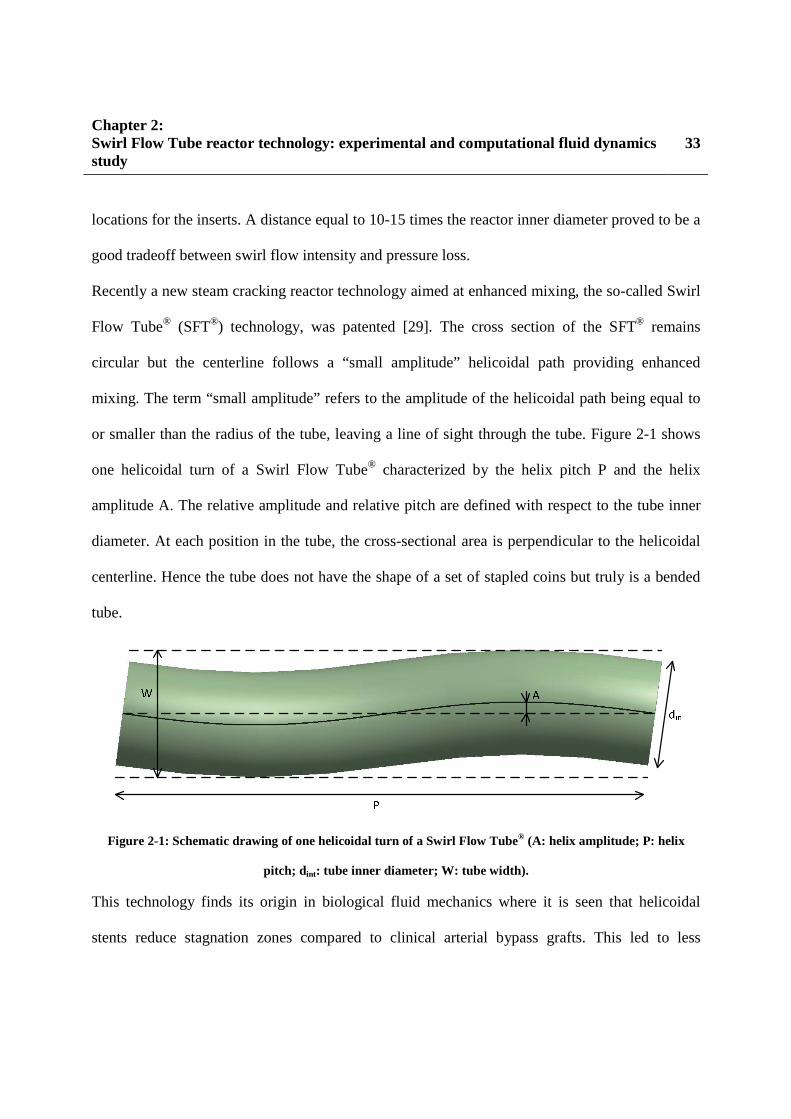
Chapter 2: Swirl Flow Tube reactor technology: experimental and computational fluid dynamics study
33
locations for the inserts. A distance equal to 10-15 times the reactor inner diameter proved to be a
good tradeoff between swirl flow intensity and pressure loss.
Recently a new steam cracking reactor technology aimed at enhanced mixing, the so-called Swirl
Flow Tube® (SFT®) technology, was patented [29]. The cross section of the SFT® remains
circular but the centerline follows a “small amplitude” helicoidal path providing enhanced
mixing. The term “small amplitude” refers to the amplitude of the helicoidal path being equal to
or smaller than the radius of the tube, leaving a line of sight through the tube. Figure 2-1 shows
one helicoidal turn of a Swirl Flow Tube® characterized by the helix pitch P and the helix
amplitude A. The relative amplitude and relative pitch are defined with respect to the tube inner
diameter. At each position in the tube, the cross-sectional area is perpendicular to the helicoidal
centerline. Hence the tube does not have the shape of a set of stapled coins but truly is a bended
tube.
Figure 2-1: Schematic drawing of one helicoidal turn of a Swirl Flow Tube® (A: helix amplitude; P: helix
pitch; d int: tube inner diameter; W: tube width).
This technology finds its origin in biological fluid mechanics where it is seen that helicoidal
stents reduce stagnation zones compared to clinical arterial bypass grafts. This led to less
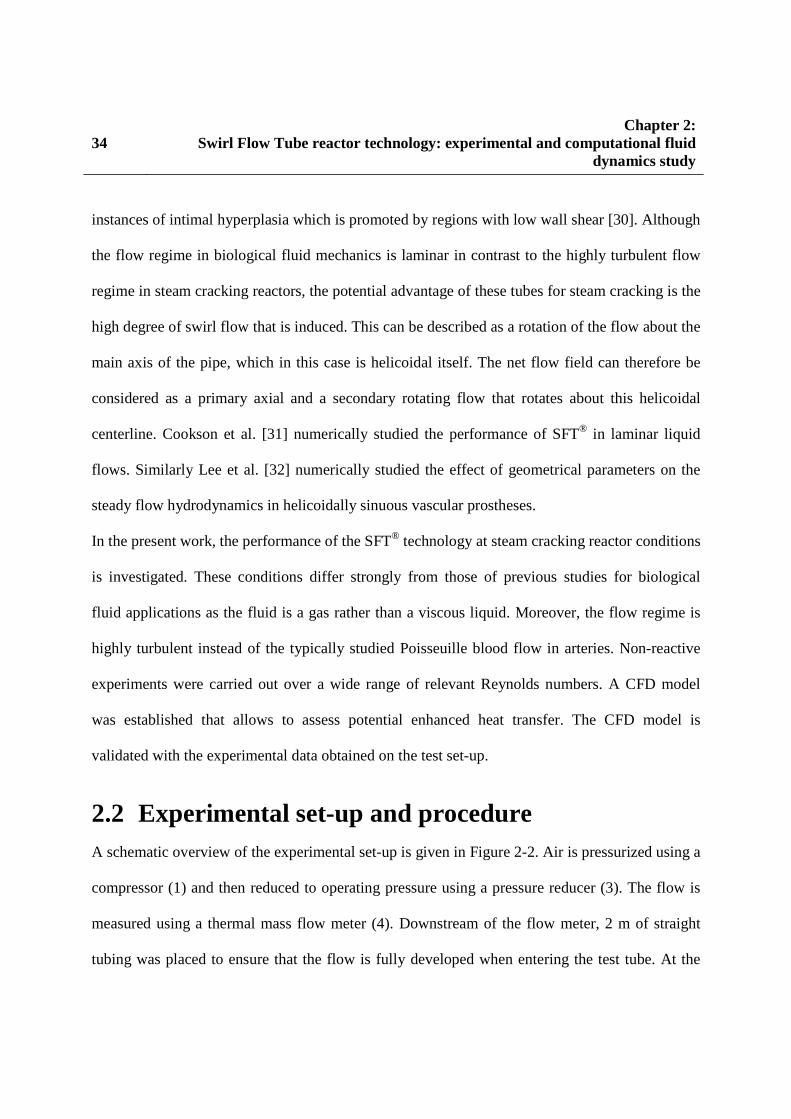
34 Chapter 2:
Swirl Flow Tube reactor technology: experimental and computational fluid dynamics study
instances of intimal hyperplasia which is promoted by regions with low wall shear [30]. Although
the flow regime in biological fluid mechanics is laminar in contrast to the highly turbulent flow
regime in steam cracking reactors, the potential advantage of these tubes for steam cracking is the
high degree of swirl flow that is induced. This can be described as a rotation of the flow about the
main axis of the pipe, which in this case is helicoidal itself. The net flow field can therefore be
considered as a primary axial and a secondary rotating flow that rotates about this helicoidal
centerline. Cookson et al. [31] numerically studied the performance of SFT® in laminar liquid
flows. Similarly Lee et al. [32] numerically studied the effect of geometrical parameters on the
steady flow hydrodynamics in helicoidally sinuous vascular prostheses.
In the present work, the performance of the SFT® technology at steam cracking reactor conditions
is investigated. These conditions differ strongly from those of previous studies for biological
fluid applications as the fluid is a gas rather than a viscous liquid. Moreover, the flow regime is
highly turbulent instead of the typically studied Poisseuille blood flow in arteries. Non-reactive
experiments were carried out over a wide range of relevant Reynolds numbers. A CFD model
was established that allows to assess potential enhanced heat transfer. The CFD model is
validated with the experimental data obtained on the test set-up.
2.2 Experimental set-up and procedure A schematic overview of the experimental set-up is given in Figure 2-2. Air is pressurized using a
compressor (1) and then reduced to operating pressure using a pressure reducer (3). The flow is
measured using a thermal mass flow meter (4). Downstream of the flow meter, 2 m of straight
tubing was placed to ensure that the flow is fully developed when entering the test tube. At the

Chapter 2: Swirl Flow Tube reactor technology: experimental and computational fluid dynamics study
35
inlet of the test tube, the temperature and pressure were measured using a PT100 Resistive
Temperature Device (6) and a water manometer (5). The test tube was 4 m long and had an
internal and external diameter of 28 · 10-3 and 32 · 10-3 m respectively.
Figure 2-2: Schematic of the experimental set-up for evaluation of heat transfer enhancement (1: compressor,
2: valve, 3: pressure reducer, 4: flow meter, 5: manometer, 6: thermocouple, 7: shell and tube heat exchanger,
8: static mixer, 9: thermocouple).
Three test tubes were used: a straight tube (Straight), a mild Swirl Flow Tube® (SFT-M) and a
high Swirl Flow Tube® (SFT-H). The geometry definitions of the tubes are given in Table 1.
Table 1: Geometry definitions of adopted test tubes.
STRAIGHT SFT-M SFT-H
Inside diameter [m] 0.028 0.028 0.028
Outside diameter [m] 0.032 0.032 0.032
Relative amplitude [-] - 0.2179 0.2964
Relative pitch [-] - 10.22 7.78
Absolute amplitude [m] - 0.0061 0.0083
Absolute pitch [m] - 0.2862 0.2178
Helix angle [°] - 7.63 13.47

36 Chapter 2:
Swirl Flow Tube reactor technology: experimental and computational fluid dynamics study
Two sets of experiments were performed; 14 pressure-drop experiments and 14 heat-transfer
experiments. The inlet Reynolds number was varied between 30,000 and 120,000. During the
pressure-drop experiments the test tube was operated adiabatically as no heating was applied and
all tubing was insulated. For the heat-transfer experiments, a shell and tube heat exchanger
configuration was applied by placing a steam jacket (7) around the test tube, keeping the test tube
outer wall temperature at 373.15 K. Only the last 2 m of the test tube were heated to avoid
asymptotic heating while the first 2 m were insulated. At the test tube outlet the temperature was
again measured using a PT100 thermocouple (9). A static mixer was placed just before this
thermocouple to ensure measurement of the mixing cup temperature. To compare the
performance of different test tubes the classical approach based on characteristic numbers is used
in line with previous works [33, 34].
For the pressure-drop experiments, the experimental data are compared in terms of Reynolds
number and Fanning friction factor. The pressure drop along a straight tube can be estimated with
the Darcy-Weisbach equation as denoted in the following equation:
�� = 4�� ��� �|��|� = 4�� ���12 ���� �� 1� (2.1)
Hence the pressure drop along the test tube as measured experimentally can be used to determine
the Fanning friction factor, according to;
�� = �����2� � ����� (2.2)

Chapter 2: Swirl Flow Tube reactor technology: experimental and computational fluid dynamics study
37
For the heat-transfer experiments, the experimental data are compared in terms of Reynolds and
Nusselt numbers. The amount of energy transferred to the air equals:
Q = ��������� !� " � !�# (2.3)
This amount of energy can also be estimated in heat-transfer terms as:
Q = $���%&�'�( (2.4)
Where for the calculation of the LMTD, it is assumed that the wall temperature is uniformly
equal to 373.15 K as a steam jacket is placed around the test tube.
The Nusselt number is defined by the following equation:
)� = &��* (2.5)
By combination of equation (2.3), (2.4),(2.5) and (2.7), the Nusselt number can be expressed as:
)� = ���+����� !� " � !�#$*�%�'�( (2.6)
All fluid properties like density, viscosity, thermal conductivity and specific heat are calculated
as the average of their values at the measured inlet and the outlet temperature.
2.3 Numerical simulation procedure
Mathematical model 2.3.1
For all simulations the steady-state condition has been considered. The 3D turbulent flow field in
the test tube is based on the solution of the RANS equations in compressible formulation. The
steady-state governing equations for continuity, momentum and energy respectively, are the
following:

38 Chapter 2:
Swirl Flow Tube reactor technology: experimental and computational fluid dynamics study
∇ ∙ ��./# = 0 (2.7)
∇ ∙ ��././# = "∇� + ∇ ∙ 2 (2.8)
∇ ∙ 4./��5 + �#6 = ∇ ∙ 7*!��∇� " 8ℎ :< = (2.9)
Equation (2.8) is closed using the Reynolds Stress Model (RSM). The superior performance of
this model compared to isotropic eddy-viscosity models is well known for flows with highly
anisotropic Reynolds stresses as is the case of swirling flow [35, 36]. In this study also, a better
agreement to experimental data was found using RSM compared to the more standard k-ε
models. To avoid initial divergence of the simulations, the standard k-ε turbulence model was
first used for 1000 iterations after which was switched to the RSM model.
To properly resolve the viscosity affected near-wall region, a two-layer model was adopted. This
model has been shown suitable for swirling flow [34, 37]. In this model, the domain is subdivided
into a viscosity-affected region and a fully turbulent region by evaluation of a wall-distance-
based turbulent Reynolds number, Rey defined as:
>?@ = �A√CD (2.10)
where y is the distance between the cell center and the nearest wall cell.
In the fully turbulent region (Rey>200) the RSM equations are used. In the viscosity affected
region (Rey<200), the one-equation model of Wolfshtein [38] is adopted. Continuity between the
two regions is provided by the blending equation of Jongen [39].

Chapter 2: Swirl Flow Tube reactor technology: experimental and computational fluid dynamics study
39
Grid generation 2.3.2
Figure 2-3 shows the grid of the test tube cross section. The mesh was generated using Gambit
2.4.6. The thickness of wall-adjacent cells equals 10 µm to ensure a y+ around 1-2 for all
simulations as necessary for the Wolfshtein model. This cross-sectional grid was then extruded
along the test tube centerline, i.e. a line for the straight tube and a helix for the Swirl Flow
Tubes®. Important to note is that the cross-sectional area is perpendicular to the centerline inside
the tube as is the case for the experimentally tested Swirl Flow Tubes®. Hence, the tube does not
have the shape of stapled coins but truly is a bended tube. Mesh independence tests showed that a
cell size of 0.8 mm in both axial as tangential direction was necessary. For all test tubes this
resulted in more than 15 million cells.
Figure 2-3: Cross-sectional grid mesh of the computational domain.

40 Chapter 2:
Swirl Flow Tube reactor technology: experimental and computational fluid dynamics study
Boundary conditions 2.3.3
In the experimental set-up a developing tube is placed upstream of the test tube leading to fully
developed flow at the inlet. Therefore a straight tube of 1 m is placed before the test tube in the
simulation grid to avoid entrance effects and to assure fully developed flow. For the air inlet
boundary the total mass flow rate is specified. As the outlet flow leaves to the atmosphere, a
pressure outlet condition equal to 101325 Pa is specified at the outlet boundary. All walls are
assumed to be smooth and a no-slip condition was adopted. An isotropic, uniform distribution for
the inlet and outlet boundary condition variables was assumed. The Reynolds stresses at the inlet
were assumed to be uniform and isotropic and calculated from the following empirical
correlations [34] for turbulence intensity and turbulence length scale for fully developed flow:
E = 0.16>?HIJ (2.11)
K = 0.07�� (2.12)
with dint the tube inner diameter.
Numerical solution 2.3.4
The governing equations were solved numerically using the commercial CFD code FLUENT
13.0 which is based on the finite volume method. The SIMPLE scheme was used for pressure-
velocity coupling. The QUICK scheme was used for the spatial discretization of all variables. As
no convergence issues were experienced default relaxation factors were adopted. Convergence
was judged by monitoring residuals, inlet pressure and outlet temperature. The residual
convergence criterion was set to 10-6 for all equations, only the energy equation criterion was set

Chapter 2: Swirl Flow Tube reactor technology: experimental and computational fluid dynamics study
41
lower to 10-9. Furthermore the inlet pressure and outlet temperature were monitored and they
were seen to change less than 1 Pa and 0.05 K respectively over the last 50 iterations for all
simulations.
2.4 Results and discussion
Experimental results 2.4.1
Pressure-drop experiments
Figure 2-4 shows the experimental Fanning friction factors for all three test tubes and the
correlation proposed by Chen et al. [40] for straight tubes with the tube surface roughness 5M set
equal to 0:
��N�OO�5M, ��, >?# = 0.331369KS T0.269796�� " 2.1911KS U0.353895 U 5M��X + 5.8506>?Y.JZJIX>? [
�
(2.13)
Comparing the Swirl Flow Tubes® with the straight tube for Reynolds numbers of 35,000 to
110,000 an increase in Fanning friction factor compared to Straight by a factor of about 2.2 to
1.4 and of 2.5 to 1.8 is observed for SFT-M and SFT-H respectively.

42 Chapter 2:
Swirl Flow Tube reactor technology: experimental and computational fluid dynamics study
Figure 2-4: Fanning friction factor as a function of inlet Reynolds number for pressure-drop experiments:
experimental values: - Straight; - SFT-M; - SFT-H, Chen correlation by Eq. (2.13): - Ea = 0
m; - Ea = 13.4 µm).
The experimental values for the straight tube are underpredicted by the correlation when
assuming a tube surface roughness equal to 0. This is caused by the experimental tube not being
ideally smooth. As all CFD simulations are performed for smooth tubes, a correction factor needs
to be applied for comparison with experimental Fanning friction factors. As the tube roughness is
unknown, the tube roughness in equation (2.13) is calibrated to the experimental data for the
straight tubes using the following equation:
2 4 6 8 10 12 14
x 104
0
0.002
0.004
0.006
0.008
0.01
0.012
0.014
0.016
Reynolds number [-]
Fan
ning
fric
tion
fact
or [
-]
StraightSFT-MSFT-HChen 0µmChen 13.4µm

Chapter 2: Swirl Flow Tube reactor technology: experimental and computational fluid dynamics study
43
min_` 87��,!a� " ��,N�OO�5M, ��, >?#��,!a� =�b
cI (2.14)
By solving equation (2.14), an absolute roughness of 13.4 µm is found. This roughness is
assumed to be the roughness of all test tubes and is in line with the typical roughness of fresh
steel tubes [41]. Hence, all Fanning friction factors calculated from CFD simulations are
multiplied with the following correction factor for comparison with experimental Fanning friction
factors:
d���, >?# = ��N�OO�13.4 ∙ 10He, ��, >?#��N�OO�0, �� , >?# (2.15)
��f� = ��ghi ∙ d���, >?# (2.16)
Based on the pressure-drop experiments the SFT-M tube has higher potential for steam cracking
applications because of the reduced pressure drop compared to the SFT-H tube. Higher pressures
affect light olefin selectivity [42], and hence, strongly influence the steam cracking economics.
Heat-transfer experiments
Figure 2-5 shows the experimental Nusselt numbers for all three test tubes and the correlation
proposed by Gnielinski et al. [43] for straight tubes:
)� = �j/8#�>? " 1000#lm1 + 12.7�j/8#I/��lm�/n " 1# (2.17)
where j = �1.82Kop�>?# " 1.64#H�.
Comparing the Swirl Flow Tubes® with the straight tube for Reynolds numbers from 30,000 to
110,000 an increase in Nusselt number compared to Straight by a factor of 1.26 to 1.22 and from

44 Chapter 2:
Swirl Flow Tube reactor technology: experimental and computational fluid dynamics study
1.49 to 1.45 is observed for SFT-M and SFT-H respectively. The better heat transfer for the SFT-
H tube will result in lower wall temperatures in steam cracking reactors, and hence, in line with
the coking model of Plehiers and Froment [44], this can result in lower coking rates if the
concentrations of coke precursors are identical. Taking into account these considerations the
SFT-H tube would be preferred to the SFT-M tube for steam cracking purposes if reduced coke
formation is taken as sole criterion.
Furthermore it is seen that the Gnielinski correlation overpredicts the experimentally obtained
values for the straight tube. However the agreement provides sufficient accuracy for the scope of
this work.
Figure 2-5: Global Nusselt number as a function of inlet Reynolds number for heat-transfer experiments:
experimental values: - Straight; - -SFT-M; - SFT-H, lines: - Gnielinski correlation by Eq.
(2.17).

Chapter 2: Swirl Flow Tube reactor technology: experimental and computational fluid dynamics study
45
Simulation results 2.4.2
Pressure drop
Figure 2-6 shows a comparison between experimental and simulated Fanning friction factors for
all 14 pressure-drop experiments. In general the agreement is good with average relative
deviations equal to 2.5, 4.4 and 2.4 % for the straight, SFT-M and SFT-H test tube respectively.
For the straight tube the largest deviations are obtained at the lowest and highest Reynolds
numbers which is in agreement with the deviations of the Chen correlation to the experimental
results as shown in Figure 2-4.
Figure 2-7A and B show the velocity magnitude in a cross section at different axial positions
along test tube SFT-M at an inlet Reynolds number of 21,740 and 115,270 respectively. As the
centrifugal force acts on the fluid, the position of maximum velocity magnitude shifts closer to
the tube wall as can be seen in Figure 2-7A. After 6 pitches the velocity field breaks up into two
vortices creating a C-shaped region of high velocity while a local minimum is created close to the
tube wall where the two vortices touch and leave the tube inner wall as described by Cookson et
al. for laminar flow [31]. Comparing the velocity fields in the cross section after 6 and 12 pitches,
it is observed that the shape of the velocity field in a cross-section no longer changes as fully-
developed turbulent flow is established. Comparing Figure 2-7A and B the shape of the velocity
magnitude continues to change so no fully developed flow is yet established at the highest
adopted Reynolds number.

46 Chapter 2:
Swirl Flow Tube reactor technology: experimental and computational fluid dynamics study
Figure 2-6: Fanning friction factor as a function of Reynolds number for pressure-drop experiments;
experimental values: - Straight; - SFT-M; - SFT-H and simulated values: - Straight; -
SFT-M; - SFT-H.
Figure 2-7: Velocity (m/s) field at an inlet Reynolds number of (A) 21·103 (B) 115·103 at different axial
positions along test tube SFT-M (from left to right: after 0, 3, 6, 9 and 12 pitches).
2 4 6 8 10 12 14
x 104
0
0.005
0.01
0.015
Reynolds number [-]
Fan
nin
g fr
ictio
n fa
ctor
[-]
Straight expSFT-M expSFT-H expStraight simSFT-M simSFT-H sim

Chapter 2: Swirl Flow Tube reactor technology: experimental and computational fluid dynamics study
47
Figure 2-8 shows the wall shear stress in a cross section at four axial positions along the
azimuthal coordinate of the cross section. The changing velocity field has a profound effect on
the wall shear stress. After 3 pitches, the wall shear stress profile has a rather broad maximum
corresponding to the broad velocity maximum close to the wall seen in the second cross section
of Figure 2-7A. However, after 6 pitches a narrow minimum in the wall shear stress profile is
simulated. This minimum corresponds to the local velocity minimum seen in the cross sections of
Figure 2-7A.
Figure 2-8: Wall shear stress as a function of azimuthal coordinate at an inlet Reynolds number of 21·103 at
different axial positions along test tube SFT-M; after 3 (A), 6 (B), 9 (C) and 12 (D) pitches.
-3 -2 -1 0 1 2 30
0.2
0.4
0.6
0.8
1
Azimuthal coordinate [rad]
Wal
l she
ar s
tress
[Pa
]
-3 -2 -1 0 1 2 30
0.2
0.4
0.6
0.8
1
Azimuthal coordinate [rad]
Wal
l she
ar s
tress
[Pa
]
-3 -2 -1 0 1 2 30
0.2
0.4
0.6
0.8
1
Azimuthal coordinate [rad]
Wal
l she
ar s
tress
[Pa
]
-3 -2 -1 0 1 2 30
0.2
0.4
0.6
0.8
1
Azimuthal coordinate [rad]
Wal
l she
ar s
tress
[Pa]

48 Chapter 2:
Swirl Flow Tube reactor technology: experimental and computational fluid dynamics study
Heat transfer
Figure 2-9 shows a comparison between experimental and simulated Nusselt numbers for all 14
heat-transfer experiments. A general overprediction is simulated with average relative deviations
equal to 13.4, 9.4 and 8.1 % for the Straight, SFT-M and SFT-H test tube respectively. As the
simulated results for the straight tube are in good agreement with the Gnielinski correlation and
the relative errors for the SFT-M and SFT-H are lower than for the straight tube, the simulated
results are considered to provide sufficient accuracy.
Figure 2-9: Nusselt number as a function of Reynolds number for heat-transfer experiments; experimental
values; - Straight; - SFT-M; - SFT-H and simulated values: - Straight; - SFT-M;
- SFT-H.
Figure 2-10A and B show the temperature of the air at several axial positions for an inlet
Reynolds number of 23·103 and 113·103 respectively. Comparing with Figure 2-7, a high
0 2 4 6 8 10 12
x 104
0
50
100
150
200
250
300
Reynolds number [-]
Nu
sse
lt n
um
be
r [-
]
Straight expSFT-M expSFT-H expStraight simSFT-M simSFT-H sim

Chapter 2: Swirl Flow Tube reactor technology: experimental and computational fluid dynamics study
49
similarity between the temperature and velocity field can be noted. First the minimum in
temperature is shifted towards the tube wall as is the velocity magnitude maximum in Figure 2-7.
After several helices as the velocity profile breaks up into two vortices, the temperature profile
shows a C-shaped region of low temperature corresponding to the C-shaped region of high
velocity in Figure 2-7. A region of higher temperature is created close to the tube wall
corresponding to the low velocity regions seen in Figure 2-7. Comparing the low and high inlet
Reynolds number simulations in Figure 2-10, a faster development of the C-shaped region is
noted.
Figure 2-10: Temperature (K) at an inlet Reynolds number of (A) 23·103 (B) 111·103 at different axial
positions along test tube SFT-M (from left to right: 0, 0.5, 1, 1.5 and 2 m).

50 Chapter 2:
Swirl Flow Tube reactor technology: experimental and computational fluid dynamics study
Figure 2-11 and Figure 2-12 show respectively the heat flux profile and the wall shear stress at
the tube inner wall at several axial positions for the straight and SFT-M test tube. Comparing the
wall shear stress and the heat flux profile shapes, large similarity is again seen. At positions with
high wall shear stress, high heat fluxes are located due to the gas scouring the tube inner wall,
reducing the boundary layer thickness. At the positions where the narrow minimum in wall shear
stress occurs a similar minimum in heat flux is located. Comparing the profiles for both the wall
shear stress and the heat flux for the Straight and the SFT-M test tube, it is seen that the minima
for the SFT-M test tube are lower than the uniform value simulated for the straight tube, however
the main part of the SFT-M profiles is higher than their counterpart in the Straight test tube. This
results in higher average values for the SFT-M as also shown on Figure 2-11. The higher heat
transfer and higher pressure drop for the SFT® can thus be attributed to the higher average wall
shear stress due to the higher velocities close to the tube wall. Further downstream the tube, the
heat flux values of the Straight tube get closer to the SFT-M values as the air temperature in the
SFT-M is higher downstream due to better heat transfer resulting in a lower driving force for heat
transfer as the wall temperature is uniform along the tube.
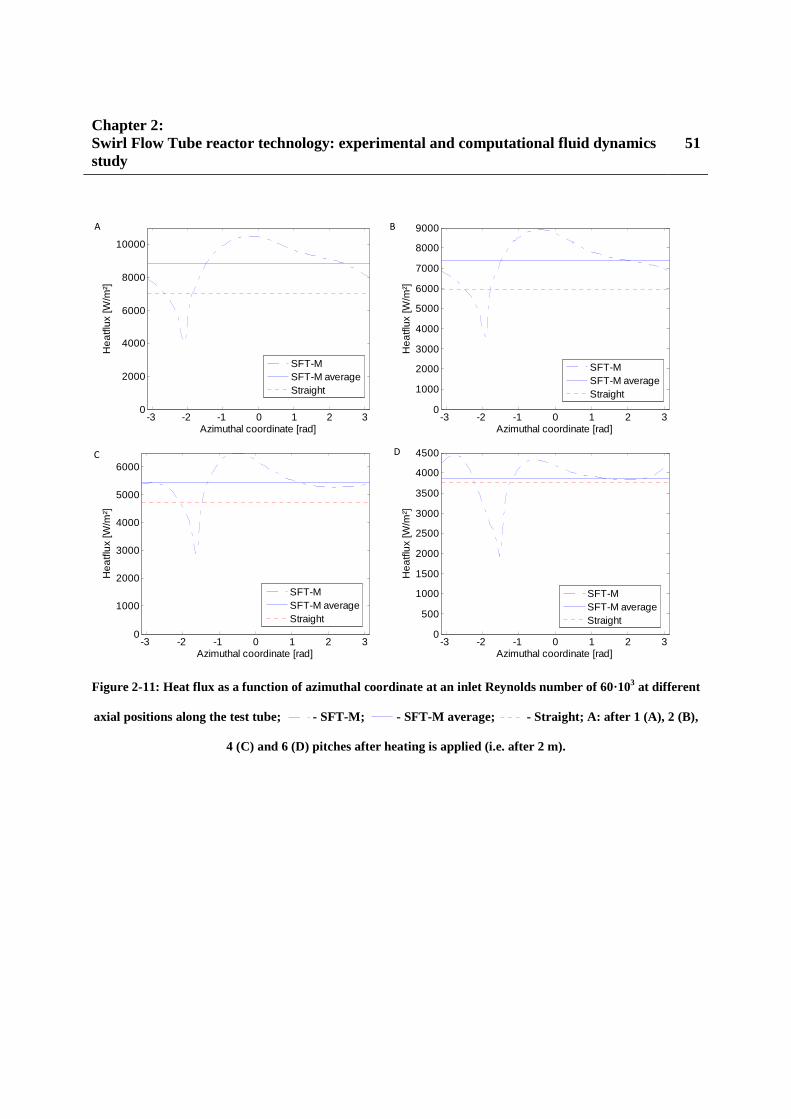
Chapter 2: Swirl Flow Tube reactor technology: experimental and computational fluid dynamics study
51
Figure 2-11: Heat flux as a function of azimuthal coordinate at an inlet Reynolds number of 60·103 at different
axial positions along the test tube; - SFT-M; - SFT-M average; - Straight; A: after 1 (A), 2 (B),
4 (C) and 6 (D) pitches after heating is applied (i.e. after 2 m).
-3 -2 -1 0 1 2 30
2000
4000
6000
8000
10000
Azimuthal coordinate [rad]
He
atfl
ux [W
/m²]
SFT-MSFT-M averageStraight
-3 -2 -1 0 1 2 30
1000
2000
3000
4000
5000
6000
7000
8000
9000
Azimuthal coordinate [rad]
He
atfl
ux [W
/m²]
SFT-MSFT-M averageStraight
-3 -2 -1 0 1 2 30
500
1000
1500
2000
2500
3000
3500
4000
4500
Azimuthal coordinate [rad]
He
atfl
ux
[W/m
²]
SFT-MSFT-M averageStraight
-3 -2 -1 0 1 2 30
1000
2000
3000
4000
5000
6000
Azimuthal coordinate [rad]
He
atfl
ux
[W/m
²]
SFT-MSFT-M averageStraight
A
C
B
D
52 Chapter 2:
Swirl Flow Tube reactor technology: experimental and computational fluid dynamics study
Figure 2-12: Wall shear stress in a cross section at an inlet Reynolds number of 60·103 at different axial
positions along the test tube; ; - SFT-M; - SFT-M average; - Straight; after 1 (A), 2 (B), 4 (C)
and 6 (D) pitches after heating is applied (i.e. after 2 m).
-3 -2 -1 0 1 2 30
1
2
3
4
5
6
7
8
Azimuthal coordinate [rad]
Wa
ll S
he
ar
Str
ess
[Pa
]
SFT-MSFT-M averageStraight
-3 -2 -1 0 1 2 30
1
2
3
4
5
6
7
Azimuthal coordinate [rad]
Wa
ll S
hea
r S
tre
ss [P
a]
SFT-MSFT-M averageStraight
-3 -2 -1 0 1 2 30
1
2
3
4
5
6
Azimuthal coordinate [rad]W
all
Sh
ear
Str
ess
[Pa
]
SFT-MSFT-M averageStraight
-3 -2 -1 0 1 2 30
1
2
3
4
5
6
Azimuthal coordinate [rad]
Wa
ll S
hea
r S
tre
ss [P
a]
SFT-MSFT-M averageStraight
A
C
B
D

Chapter 2: Swirl Flow Tube reactor technology: experimental and computational fluid dynamics study
53
To assess the uniformity in a cross section, a weighed temperature variance is calculated from the
discrete temperatures from the computational surfaces at the tube cross section:
q∑ ��,4� " �Mst6�ucI ��,����Mst
(2.18)
with ��, the mass flow rate leaving the local surface i, ��,��� the total mass flow rate, � the
local gas temperature and �Mst the mixing cup temperature of the cross section. This coefficient
is shown in Figure 2-13 as a function of the axial length for the Straight, SFT-M and SFT-H test
tube at an inlet Reynolds number of 60·103. As seen from this figure, the temperature variance is
lower for the SFT® test tubes so a more uniform temperature profile is obtained by adopting a
SFT®. The SFT-H tube shows the best results at the expense of a higher pressure drop as
mentioned before. The more uniform temperature can be attributed to the stronger in-plane
mixing by the swirl flow induced by the SFT® and the higher heat transfer rate.

54 Chapter 2:
Swirl Flow Tube reactor technology: experimental and computational fluid dynamics study
Figure 2-13: Mixing cup weighted temperature variance as a function of the axial coordinate for the heat-
transfer experiments: - Straight; - SFT-M; - SFT-H.
These considerations are interesting for non-reactive flow, but are even more relevant in the case
of reactive flow in steam crackers. As a greater temperature uniformity goes coupled with greater
species concentration uniformity, a more uniform profile will provide lower coking rates and
more controlled cracking, i.e. less under- and overcracking [21]. However, the area of high
temperature close to the wall can induce a local high coke formation. Hence, the coke thickness
will not grow uniform in a cross-section. Obviously, incorporation of detailed chemistry
drastically increases computational cost [45-48]. Implementing chemical gas-phase reactions and
a coking model in the 3D flow model is discussed in Chapter 3, 4 and 5 of this thesis.
2 2.2 2.4 2.6 2.8 3 3.2 3.4 3.6 3.8 40.005
0.01
0.015
0.02
0.025
0.03
0.035
0.04
Axial coordinate [m]
Co
effi
cie
nt o
f Va
riatio
n [-
]
StraightSFT-MSFT-H

Chapter 2: Swirl Flow Tube reactor technology: experimental and computational fluid dynamics study
55
2.5 Conclusions A novel reactor design for steam cracking reactors, called Swirl Flow Tube® has been evaluated
experimentally in a newly constructed test set-up. Three test tubes were used: a straight tube, a
mild Swirl Flow Tube® (SFT-M) and a high Swirl Flow Tube® (SFT-H). For Re numbers in the
range of 30,000 – 120,000, the SFT-M tube has a lower pressure drop compared to the SFT-H
tube. However, the latter results in an increase of heat transfer by 20 % compared to the SFT-M
tube and up to 50 % compared to the straight tube. The results prove that indeed for swirl flow
reactors higher heat transfer rates can be obtained compared to conventional straight tubes at the
cost of a higher pressure drop. This is a factor 1.4 to 2.2 higher depending on Reynolds number
and geometry.
A CFD model was adopted that is able to capture the main flow properties of the SFT®. Mesh
independence tests showed that a cell size of 0.8 mm in both axial as tangential direction was
necessary, resulting in meshes of more than 15 million cells. The increased heat transfer and
pressure drop result from a higher wall shear stress. A narrow area of low velocity and high
temperature close to the tube wall is simulated. The effect of the latter on coke formation on the
reactor wall in processes like steam cracking can be accounted for by implementing a gas-phase
reaction model and a coking model. This is discussed further in Chapter 3, 4 and 5 of this thesis.

56 Chapter 2:
Swirl Flow Tube reactor technology: experimental and computational fluid dynamics study
References [1] T. Ren, B. Daniëls, M.K. Patel, K. Blok, Petrochemicals from oil, natural gas, coal and biomass: Production costs in 2030–2050, Resources, Conservation and Recycling, 53 (2009) 653-663. [2] T. Ren, M.K. Patel, K. Blok, Steam cracking and methane to olefins: Energy use, CO2 emissions and production costs, Energy, 33 (2008) 817-833. [3] S. Wauters, G.B. Marin, Kinetic Modeling of Coke Formation during Steam Cracking, Industrial & Engineering Chemistry Research, 41 (2002) 2379-2391. [4] K.M. Van Geem, R. Zajdlik, M.F. Reyniers, G.B. Marin, Dimensional analysis for scaling up and down steam cracking coils, Chemical Engineering Journal, 134 (2007) 3-10. [5] J. Wang, M.-F. Reyniers, K.M. Van Geem, G.B. Marin, Influence of silicon and silicon/sulfur-containing additives on coke formation during steam cracking of hydrocarbons, Industrial & Engineering Chemistry Research, 47 (2008) 1468-1482. [6] H. Zimmermann, R. Walzl, Ethylene, in: Ullmann's Encyclopedia of Industrial Chemistry, Wiley-VCH Verlag GmbH & Co. KGaA, 2000. [7] E. Ranzi, M. Dente, S. Pierucci, S. Barendregt, P. Cronin, Coking simulation aids on-stream time, Oil & Gas Journal, 83 (1985) 49-52. [8] R.E. Lobnig, H.J. Grabke, Mechanisms of simultaneous sulfidation and oxidation of Fe-Cr and Fe-Cr-Ni-alloys and of the failure of protective chromia scales, Corrosion Science, 30 (1990) 1045-1071. [9] M. Bajus, J. Baxa, Coke formation during the pyrolysis of hydrocarbons in the presence of sulfur-compounds, Collection of Czechoslovak Chemical Communications, 50 (1985) 2903-2909. [10] W. Anon, New additive retards coke formation in ethylene furnace tubes, Oil & Gas Journal, 92 (1994) 73-75. [11] K.K. Ghosh, D. Kunzru, Sodium-silicate as a coke inhibitor during naphtha pyrolysis, Canadian Journal of Chemical Engineering, 70 (1992) 394-397. [12] A.G. Goossens, M. Dente, E. Ranzi, Improve steam cracker operation, Hydrocarbon Processing, 57 (1978) 227-236. [13] P. Das, S. Prasad, D. Kunzru, Organophosphorus compounds as coke inhibitors during naphtha pyrolysis - effect of benzyl diethyl phosphite and triphenylphosphine sulfide, Industrial & Engineering Chemistry Research, 31 (1992) 2251-2255. [14] S. Vaish, D. Kunzru, Triphenyl phosphite as a coke inhibitor during naphtha pyrolysis, Industrial & Engineering Chemistry Research, 28 (1989) 1293-1299. [15] H.M. Woerde, S. Barendregt, F. Humblot, C. Brun, Mitigate coke formation, Hydrocarbon Processing, 81 (2002) 45-50. [16] I. Dhuyvetter, M.-F. Reyniers, G.F. Froment, G.B. Marin, D. Viennet, The influence of dimethyl disulfide on naphtha steam cracking, Industrial & Engineering Chemistry Research, 40 (2001) 4353-4362.

Chapter 2: Swirl Flow Tube reactor technology: experimental and computational fluid dynamics study
57
[17] M.-F. Reyniers, G.F. Froment, Influence of metal-surface and sulfur addition on coke deposition in the thermal-cracking of hydrocarbons, Industrial & Engineering Chemistry Research, 34 (1995) 773-785. [18] D.E. Brown, J.T.K. Clark, A.I. Foster, J.J. McCarroll, M.L. Sims, Inhibition of coke formation in ethylene steam cracking, Acs Symposium Series, 202 (1982) 23-43. [19] P. Broutin, F. Ropital, M.-F. Reyniers, G.F. Froment, Anticoking coatings for high temperature petrochemical reactors, Oil & Gas Science and Technology - Revue D'Institut Français du Pétrole Energies Nouvelles, 54 (1999) 375-385. [20] S.B. Parks, C.M. Schillmoller, Use alloys to improve ethylene production, Hydrocarbon Processing, 75 (1996) 53-&. [21] J.J. De Saegher, T. Detemmerman, G.F. Froment, Three dimensional simulation of high severity internally finned cracking coils for olefins production, Revue De L'Institut Français Du Pétrole, 51 (1996) 245-260. [22] T. Detemmerman, G.F. Froment, Three dimensional coupled simulation of furnaces and reactor tubes for the thermal cracking of hydrocarbons, Revue De L'Institut Français Du Pétrole, 53 (1998) 181-194. [23] M. Györffy, M. Hineno, H. Kunihude, P. Seong-Hoan, Y. Min-Soo, MERT performance and technology update, AIChE Spring Meeting: Ethylene producers meeting, Tampa Bay, US, 2009, pp. 7. [24] A. Carrillo, Intensified Heat Transfer technology - CFD analysis to explain how and why IHT increases runlength in commercial furnaces, AIChE Spring Meeting 2010: Ethylene producers meeting, San Antonio, TX, 2010. [25] D.J. Brown, Internally finned radiant coils: a valuable tool for improving ethylene plant economics, 6th EMEA Petrochemicals Technology Conference, London, U.K., 2004. [26] K.M. Van Geem, G.J. Heynderickx, G.B. Marin, Effect of radial temperature profiles on yields in steam cracking, AIChE Journal, 50 (2004) 173-183. [27] G.H. Hu, H.G. Wang, F. Qian, Y. Zhang, J.L. Li, K.M. Van Geem, G.B. Marin, Comprehensive CFD Simulation of Product Yields and Coking Rates for a Floor- and Wall-Fired Naphtha Cracking Furnace, Industrial & Engineering Chemistry Research, 50 (2011) 13672-13685. [28] T. Torigoe, K. Hamada, M. Furuta, M. Sakashita, K. Otsubo, M. Tomita, Mixing element radiant tube (MERT) improves cracking furnace performance, 11th Ethylene Producers' Conference, Houston, TX, 1999. [29] C.G. Caro, P.L. Birch, W. Tallis, Olefin production furnace with a helical tube, T. S.A.S., European Patent Source, (2010). [30] C.G. Caro, N.J. Cheshire, N. Watkins, Preliminary comparative study of small amplitude helical and conventional ePTFE arteriovenous shunts in pigs, J. R. Soc. Interface, 2 (2005) 261-266. [31] A.N. Cookson, D.J. Doorly, S.J. Sherwin, Mixing Through Stirring of Steady Flow in Small Amplitude Helical Tubes, Annals of Biomedical Engineering, 37 (2009) 710-721. [32] K.E. Lee, J.S. Lee, J.Y. Yoo, A numerical study on steady flow in helically sinuous vascular prostheses, Medical Engineering & Physics, 33 (2011) 38-46.

58 Chapter 2:
Swirl Flow Tube reactor technology: experimental and computational fluid dynamics study
[33] J.V. Albano, K.M. Sundaram, M.J. Maddock, Applications of Extended Surfaces in Pyrolysis Coils, Energy Progress, 8 (1988) 160-168. [34] M. Ahmadvand, A.F. Najafi, S. Shahidinejad, An experimental study and CFD analysis towards heat transfer and fluid flow characteristics of decaying swirl pipe flow generated by axial vanes, Meccanica, 45 (2010) 111-129. [35] A.M. Jawarneh, G.H. Vatistas, Reynolds stress model in the prediction of confined turbulent swirling flows, Journal of Fluids Engineering-Transactions of the Asme, 128 (2006) 1377-1382. [36] S.L. Yang, Y.K. Siow, B.D. Peschke, R.R. Tacina, Numerical study of nonreacting gas turbine combustor swirl flow using Reynolds stress model, J. Eng. Gas. Turbines Power-Trans. ASME, 125 (2003) 804-811. [37] A.F. Najafi, M.H. Saidi, M.S. Sadeghipour, M. Souhar, Numerical analysis of turbulent swirling decay pipe flow, International Communications in Heat and Mass Transfer, 32 (2005) 627-638. [38] M. Wolfshtein, The velocity and temperature distribution in one-dimensional flow with turbulence augmentation and pressure gradient, International Journal of Heat and Mass Transfer, 12 (1969) 301-318. [39] T. Jongen, Simulation and modeling of turbulent incompressible fluid flows, EPFL, 1998. [40] N.H. Chen, An explicit equation for friction factor in pipe, Ind. Eng. Chem. Fundam., 18 (1979) 296-297297. [41] D.W. Green, R.H. Perry, Perry's chemical engineers' handbook 8th edition, 2007. [42] K.M. Van Geem, M.F. Reyniers, G.B. Marin, Two severity indices for scale-up of steam cracking coils, Industrial & Engineering Chemistry Research, 44 (2005) 3402-3411. [43] V. Gnielinski, New equations for heat and mass-transfer in turbulent pipe and channel flow, International Chemical Engineering, 16 (1976) 359-368. [44] P.M. Plehiers, G.F. Froment, Firebox simulation of olefin units, Chemical Engineering Communications, 80 (1989) 81-99. [45] W.J. Pitz, C.J. Mueller, Recent progress in the development of diesel surrogate fuels, Progress in Energy and Combustion Science, 37 (2011) 330-350. [46] T. Lu, C.K. Law, Toward accommodating realistic fuel chemistry in large-scale computations, Progress in Energy and Combustion Science, 35 (2009) 192-215. [47] K.Y. He, M.G. Ierapetritou, I.P. Androulakis, Integration of On-The-Fly Kinetic Reduction with Multidimensional CFD, AIChE Journal, 56 (2010) 1305-1314. [48] L. Liang, J.G. Stevens, J.T. Farrell, A dynamic adaptive chemistry scheme for reactive flow computations, Proceedings of the Combustion Institute, 32 (2009) 527-534.

Chapter 3: Computational Fluid Dynamics-based design of finned steam cracking reactors
59
Chapter 3:
Computational Fluid Dynamics-based design
of finned steam cracking reactors
This chapter has been published as: C.M. Schietekat, D.J. Van Cauwenberge, K.M. Van Geem, G.B. Marin, Computational fluid dynamics-based design of finned steam cracking reactors, AIChE Journal, 60 (2014) 794-808

60 Chapter 3: Computational Fluid Dynamics-based design of finned steam cracking reactors
Abstract The use of one-dimensional reactor models to simulate industrial steam cracking reactors has
been one of the main limiting factors for the development of new reactor designs and the
evaluation of existing three-dimensional (3D) reactor configurations. Therefore a three-
dimensional computational fluid dynamics approach is proposed in which the detailed free-
radical chemistry is accounted for. As a demonstration case the application of longitudinally and
helicoidally finned tubes as steam cracking reactors was investigated under industrially relevant
conditions. After experimental validation of the modeling approach, a comprehensive parametric
study allowed to identify optimal values of the fin parameters, i.e. fin height, number of fins and
helix angle to maximize heat transfer. Reactive simulations of an industrial Millisecond propane
cracker were performed for four distinct finned reactors using a reaction network of 26 species
and 203 elementary reactions. The start-of-run external tube metal temperatures could be reduced
by up to 50 K compared to conventionally applied bare tubular reactors when applying optimal
fin parameters. Implementation of a validated coking model for light feedstocks showed that
coking rates are reduced up to 50 %. However, the increased friction and inner surface area lead
to pressure drops higher by a factor from 1.22 to 1.66 causing minor but significant shifts in light
olefin selectivity. For the optimized helicoidally finned reactor the ethene selectivity dropped,
while propene and 1,3-butadiene selectivity increased with a similar amount.
Keywords: steam cracking, CFD, olefins, coke formation, finned reactor, enhanced heat transfer

Chapter 3: Computational Fluid Dynamics-based design of finned steam cracking reactors
61
3.1 Introduction Steam cracking of hydrocarbons is the predominant commercial process for producing many
platform chemicals such as light olefins (i.e. ethene, propene and butadiene) and aromatics (i.e.
benzene, toluene and xylenes). These platform chemicals are the building blocks for most
polymers and the starting molecules for the production of many additives, solvents and other
high-value chemicals. The process is one of the most energy-intensive processes in the chemical
industry using about 8 % of the industry’s primary energy consumption [1]. This is mainly
associated with the energy consumed in the separation section, in which temperatures lower than
160 K can be encountered [2]. However, also in the furnace considerable energy efficiency
improvements are possible. Per ton high value chemicals approximately 1 ton of CO2 is produced
and depending on the cracker’s design and feedstock 10 – 15 GJ energy is consumed [1, 3]. A
major factor for the process energy efficiency is the formation of coke on the inner wall of the
tubular cracking reactors. This carbonaceous coke layer reduces the cross-sectional area and leads
to an increasing reactor pressure drop over time. The latter promotes bimolecular reactions over
monomolecular reactions, typically associated with a loss in olefin selectivity [4]. Moreover, this
coke layer is highly insulating, increasing the conductive resistance for heat transfer from the
furnace to the process gas. To maintain the same cracking severity, this increased heat transfer
resistance is compensated by increasing the fuel input to the furnace burners. This leads to higher
external tube metal temperatures (TMT). Eventually, either metallurgical constraints of the
reactor alloy or an excessive pressure drop over the reactor will force the operators to cease
production and decoke the reactors. Typically this will require production to be halted for 36-48
hours, having a considerable adverse effect on the economics of the process.

62 Chapter 3: Computational Fluid Dynamics-based design of finned steam cracking reactors
In light of this energetic and economic drawback, many efforts have been made towards the
development of technologies to reduce coke formation. These technologies can be divided into
three groups: additives, surface technologies and three-dimensional reactor configurations for
heat transfer enhancement. As additives mainly sulfur-containing components [5, 6] are used.
While a general consensus exists on the beneficial effect for the suppression of CO production,
the reported effect on coke formation is contradictory [5, 7]. For metal surface technologies, low-
coking alloys [8, 9] and (catalytic) coatings [10-15] are typically studied.
In this chapter, the focus is on the third group, i.e. the application of three-dimensional reactor
configurations. By means of improved heat transfer, lower temperatures at the coke-gas interface
and thus lower coking rates are obtained compared to conventional tubular reactors.
Alternatively, the reactor throughput and the furnace fuel flow rate could be increased while
maintaining the tube skin temperature. One such three-dimensional reactor configuration is the
use of longitudinal or helicoidal fins on the reactor tube inner surface, allowing improved heat
transfer mainly because of an increased internal surface area.
Although the literature on this topic for heat exchanger applications is extensive [16-18], the
characteristics of the flow inside finned tubes are still not well understood due to the limited
availability of accurate experimental data [18]. Water flow visualization studies indicate the
existence of different regimes, depending on the angle between the fins and the tube axis [17, 19].
For helix angles smaller than 30° and for relatively tall and few fins, a rotational pattern
dominates as the flow follows the space in between the fins and swirling flow, i.e. a large
azimuthal velocity component, is established. However, when using larger helix angles the flow
is seen to be prone to coring, i.e. the main portion of the flow is constrained to the core of the

Chapter 3: Computational Fluid Dynamics-based design of finned steam cracking reactors
63
tube. A number of correlations for the Nusselt numbers and friction factors of these tubes have
already been proposed, but none of these are valid over the entire range of fin dimensions and
Reynolds numbers [18].
While in heat exchangers a wide variety of fin shapes is used, the fins typically applied in
pyrolysis reactors are rounded fins with a smooth concave-convex structure in order to avoid
flow separation and possible local hot spots for coke formation. Figure 3-1 shows the cross
section of the adopted tubes. The geometric parameters are the tube outer diameter, the maximum
inner diameter, the fin height e, the minimum metal thickness t and the fin width w. The
curvature of the fins is determined by two touching circles as shown in dashed lines in Figure
3-1. Only four parameters can be chosen independently. Typically the tube outer and maximum
inner diameter, the fin height and the number of fins are chosen. In longitudinally finned tubes,
the cross section is extruded along the tube centerline, i.e. the fins are parallel to the tube
centerline. In helicoidally finned tubes, the fins are extruded along a helix. Hence, for
helicoidally finned tubes an additional geometric parameter can be chosen, i.e. the helix angle.
This helix angle corresponds to the angle between the helicoidal fins and the tube centerline.

64 Chapter 3:
Computational Fluid Dynamics-based design of finned steam cracking reactors
Figure 3-1: Part of the cross section of a finned tube (OD: outer diameter, D: inner diameter, w: fin width, e:
fin height, t: minimum metal thickness).
A study by Brown on these geometries indicated that the heat transfer improvement for
longitudinally finned tubes follows a linear relationship with the surface area increase [20].
Albano et al. compared a longitudinally and helicoidally finned tube by performing air flow
experiments through a heated tube [21]. The Colburn j-factors for the longitudinally and
helicoidally finned tubes were found to be respectively 20 % and 40 % lower than for bare tubes.
However, this loss was offset by a 44 % increase in internal surface area compared to an
equivalent bare tube, i.e. a bare tube with the same cross-sectional surface area. The better
performance of the longitudinally finned compared to the helicoidally finned tubes was attributed
to a greater tendency of the air to bypass the fins in the latter. Pressure drops were measured to be
higher for the helicoidally finned tubes compared to longitudinally finned tubes. The latter was
confirmed by the simulation results obtained by De Saegher et al. [22] for an industrial propane

Chapter 3: Computational Fluid Dynamics-based design of finned steam cracking reactors
65
cracking reactor. In contrast to Albano et al. [21], these authors simulated a higher heat transfer
coefficient for the helicoidally finned tube compared to the corresponding longitudinally finned
tube. This was attributed to more intense mixing and reduced radial temperature gradients in the
helicoidally finned tubes. The accuracy of the results of De Saegher et al. [22] can be debated
because of the adopted coarse computational grid and the first-order discretization schemes that
were used due to much lower computational capabilities. A recent patent by Higuchi et al. [23]
covers a slightly different geometry where the fins cover only part of the tube perimeter with bare
spaces in-between. Based on CFD simulations of air flow, favorable ranges for the fin
dimensions were determined. The optimal helix angle was found to be around 25-30°, while the
optimal fin height-to-diameter ratio was determined to be between 0.1 and 0.2. Increasing the fin
height-to-width ratio was found to be favorable as more intense heating was achieved. An upper
limit of 0.7 was determined based on the limitations of the fin welding process and practical
implications for e.g. plugging of the reactor during decoking operation by spalled coke. Wolpert
et al. [24] also recently proposed helicoidally finned tubes with a lower fin height than the
aforementioned references. The authors state that this allows the generation of swirling flow in
the immediate vicinity of the fins and that this swirling flow spreads to the tube core.
The above clearly shows that in order to properly assess the full potential of finned reactors, the
influence of each of the geometric parameters needs to be investigated systematically. To the
authors’ knowledge, this has not been done before. More importantly the availability of a reliable
simulation model for 3D reactor geometries in which the free-radical gas-phase chemistry is
accounted for next to coke formation and fluid dynamics would open the door for a more rapid
evaluation of new and existing 3D reactor designs. Although many efforts have been made

66 Chapter 3: Computational Fluid Dynamics-based design of finned steam cracking reactors
towards the accurate CFD simulation of the fire-side of steam cracking units [25-34], the
literature on CFD simulations of the reactor-side is limited [22, 30, 32, 34]. Besides the work of
De Saegher et al. [22], all aforementioned references use highly simplified global reaction
networks. Only detailed free-radical reaction networks capture the essential chemistry to allow a
trustworthy prediction of the effect of reactor configuration on product yields. As mentioned
before the simulations of De Saegher et al. [22] were performed on a coarse computational grid
and adopted first-order discretization schemes. To the authors’ knowledge, no grid-independent
simulations of steam cracking reactors with higher-order discretization schemes and a free-radical
reaction network have been published. Therefore in this work the Reynolds-Averaged Navier-
Stokes (RANS) approach is combined with such a detailed single-event microkinetic model. The
first step is the validation of the CFD model using available experimental data. Secondly, the
potential of the application of internally finned tubes in steam crackers is assessed by performing
a comprehensive non-reactive parametric CFD study providing guidelines for optimal design.
Finally, optimal designs are evaluated in an industrial propane cracking Millisecond furnace. The
effect of the selected 3D reactor geometries on product selectivities and coking tendency is
evaluated. The results are validated with industrial data from a Millisecond furnace operated
under similar conditions.

Chapter 3: Computational Fluid Dynamics-based design of finned steam cracking reactors 67
3.2 CFD model setup
Governing equations 3.2.1
For a steady-state three-dimensional simulation of compressible reactive gas flow, the governing
equations are the following:
• Global continuity equation
� ∙ ����� � 0 (3.1)
• Navier-Stokes equations
� ∙ ������� � �� � � ∙ � (3.2)
• Energy equation
� ∙ ������ � ��� � � ∙ ������� ��� ���� � �� (3.3)
• Species transport equations
� ∙ ��� !� � � ∙ �" � #! , ∀' � 1, )*�+, (3.4)
In these equations �" is the diffusion flux of species ', including contributions from both the
laminar and turbulent diffusivity as well as the thermal (Soret) diffusivity. �� is the heat of
reaction, ! the concentration of species ', #! the net rate of production of species ' and )*�+,
the number of species. The performed simulations showed that in future work the laminar and
thermal diffusivity do not need to be explicitly accounted for because the turbulent diffusion is
always at least two orders of magnitude greater than the sum of both.
68 Chapter 3:
Computational Fluid Dynamics-based design of finned steam cracking reactors
Turbulence modeling 3.2.2
The flow properties are Reynolds-decomposed to a steady mean value and a fluctuating turbulent
contribution. This generates an additional stress tensor, characterizing the transfer of momentum
by turbulence, the so-called Reynolds stresses: ''ji
tij uuρτ −= . Closure for these additional
unknowns was provided by use of the Boussinesq approximation, expressing the Reynolds
stresses in terms of the mean velocities. If the transport of momentum is assumed to be a
diffusive process, an eddy viscosity can be introduced, analog to the molecular viscosity. One of
the most widely applied models for determining this eddy viscosity is the standard k-ε model,
where two additional transport equations are solved for the turbulent kinetic energy k and the
energy dissipation rate ε respectively. For swirling flow, results can be further improved by use
of the k-ε RNG model as an extra source term is introduced to the dissipation equation in regions
with large strain rate. Although at the basis of some very successful models, the Boussinesq
approximation assumes isotropic eddy viscosity. Abandoning this concept, the Reynolds stress
model (RSM) solves 6 additional transport equations for each of the components of the
symmetric Reynolds stress tensor, along with an equation for the energy dissipation rate. Given
the strong coupling between these 7 additional partial differential equations, this makes
computation much more expensive. As the RSM can model flow characteristics resulting from
anisotropy of the Reynolds stresses, more accurate results are to be expected in highly swirling
flows.
In the present work, the k-ε RNG model was used for the bare tubes and for the tubes with
longitudinal fins. For the more complex, swirling flow inside the helicoidally finned tubes the k-ε

Chapter 3: Computational Fluid Dynamics-based design of finned steam cracking reactors 69
RNG model was used for initial convergence. In a second step RSM was used because it gave a
better agreement with the experimental validation data discussed in section 3.4.
Boundary conditions 3.2.3
At the tube inlet, the temperature, mass flow rate, turbulence parameters k and ε and the
composition of the process gas were imposed. The turbulence parameters were calculated for a
turbulence intensity of 8 % and a characteristic length scale of 10 % of the tube hydraulic
diameter. At the outlet of the tube, a constant pressure boundary condition was set. All other
variables were extrapolated from the integration field. The no-slip boundary condition was set at
the tube inner walls. In order to apply this condition for highly turbulent flow, FLUENT’s
enhanced wall treatment was used to “bridge” the solution variables in the near-wall cells. This
model combines a two-layer model with enhanced wall functions by blending linear and
logarithmic laws-of-the-wall. Validity of the use of a two-layer model was ensured by placing
computational cells within the viscous sub-layer, with the near-wall cells satisfying the y+<1
condition. The energy equation was solved by imposing either a temperature or a heat flux profile
to the tube outer walls.
Chemistry model 3.2.4
Steam cracking of hydrocarbons mainly proceeds through a free-radical mechanism, which is
characterized by a vast number of species and reactions [35-38]. The incorporation of such
detailed chemical networks is computationally expensive [39]. Hence, to limit computational
cost, a network specifically geared at propane cracking was used by reducing the full single-event
microkinetic CRACKSIM model [40-42] to its relevant core for propane cracking. The final

70 Chapter 3:
Computational Fluid Dynamics-based design of finned steam cracking reactors
network consisted of 203 reactions between 26 species, of which 13 radical species. Validation of
the reduced network by comparison to the full network is provided in Appendix A.
The RMG Transport estimator was used for predicting the Lennard-Jones characteristic length
and energy parameters [43]. These were then applied in FLUENT’s kinetic theory method for
calculation of thermal conductivity and viscosity for each individual species [44, 45]. Diffusion
coefficients were quantified on this basis as well by using a modification of the Chapman-Enskog
formula [46]. Finally, thermal diffusion was taken into account by using an empirical
composition-dependent form of the Soret diffusion coefficient [47]. Properties of the multi-
component mixture were calculated by ideal gas mixing laws.
Numerical model 3.2.5
The commercial CFD code ANSYS FLUENT 13.0 was adopted to solve the governing equations.
This general-purpose CFD package uses the finite-volume method. Discretization of all equations
was achieved using the Quadratic Upstream Interpolation for Convective Kinetics (QUICK)
scheme, combining the strengths of both upwind and central differencing schemes by using a
three-point upstream quadratic interpolation. Although an unbounded scheme, it was selected
based on the reported improved accuracy for rotating and swirling flows compared to the second-
order up-wind scheme [48]. It can be proven that the scheme is third order accurate [48, 49]. The
residual convergence criterion was set to 10-6 for all equations, only the energy and species
equations were set lower to 10-9. Furthermore the inlet pressure, outlet temperature and species
concentrations were monitored. The inlet pressure and outlet temperature were seen to change
less than 1 Pa and 0.05 K respectively over the last 50 iterations for all simulations. The relative

Chapter 3: Computational Fluid Dynamics-based design of finned steam cracking reactors 71
change over the last 50 iterations of all species concentrations were seen to change less than
0.1%.
Computational grid 3.2.6
The computational grid was constructed from a 2D triangular mesh which was extruded along the
axial coordinate. For the helicoidally finned tubes a twist vector was applied to obtain the correct
helix angle. By symmetry considerations, the computational domain can be limited to one fin of
the tube to reduce computational time. Periodic boundary conditions are applied to allow flow
through the azimuthal boundaries in case of swirling flow. A fine boundary layer near the tube
inner wall is added to ensure computational cells in the viscous sub-layer having a y+ < 1 as
required by the enhanced wall treatment model. Grid independence for the tubes adopted by
Albano et al. [50] was achieved at a mesh density of approximately 5.105 and 3.105 cells/meter
for the fluid and metal volume respectively as shown in Appendix B. Grid sizes in wall units [51]
for grid independence were seen to be -./012 ∆45, ∆65, ∆758 � 950, 0.8 50, 333> . These
values were used as upper limits for all grids. These grids used in the reactive simulations were
further refined based on the temperature gradient of the converged solution. The results of this
grid refinement are also shown in Appendix B. No significant change in the results is seen by the
grid refinement. The grid independent mesh for the tubes adopted by Albano et al. [50] is shown
in Figure 3-2.

72 Chapter 3: Computational Fluid Dynamics-based design of finned steam cracking reactors
Figure 3-2: Grid independent mesh of a cross section of the tubes adopted by Albano et al. [50].
3.3 CFD model validation The CFD model was validated by comparison with the experimental results obtained by Albano
et al. [50]. By means of an experimental setup capable of measuring pressure drop and
temperature along the axial coordinate, Albano et al. evaluated the heating performance of a
longitudinally and a helicoidally finned tube. In their experimental setup, air flows through a
steam-heated finned tube containing four thermocouples to measure the air temperature in the
center of the tube at different axial positions. As the air is being released to the atmosphere, the
pressure at which the inlet diaphragm pump is operating indicates the pressure drop over the tube.
For the exact dimensions of the tubes, reference is made to the original paper of Albano et al.
[50].

Chapter 3: Computational Fluid Dynamics-based design of finned steam cracking reactors
73
The experiments with a longitudinally and a helicoidally finned tube were performed at air mass
flow rates of 0.107 and 0.103 kg/s respectively, which correspond to an inlet Reynolds number of
approximately 230 103. It is important to stress that the experiments did not involve a sufficiently
long inlet section to avoid entrance effects. In the performed CFD simulations a small inlet
section of 0.2 m length was included as the exact dimensions of the experimental inlet section are
unknown. Furthermore, the temperatures measured on the outside of the tube were flawed due to
steam condensation, leaving only the inner wall temperatures as reliable data. Hence, in the CFD
simulations the inner wall temperature profile was imposed without taking conduction through
the metal into account. The latter implies that the temperatures in the peaks and valleys were
assumed to be equal, whereas in reality they differed by 1-2 K. Air was treated as an ideal gas
with viscosity, specific heat capacity and thermal conductivity following a piecewise-linear
temperature dependence. The simulation results for pressure and temperature are compared to
experimental data in Figure 3-3 for the longitudinally and helicoidally finned tube.
Pressure drops were simulated accurately with relative errors of 3.2 % and 4.9 % for the
longitudinally and helicoidally finned tube respectively. Temperatures were underpredicted for
both tubes but it can be seen that the major difference lies in the entrance region. As the
experimental setup did not include a sufficiently long adiabatic inlet section, the deviations near
the inlet can be explained by the development of turbulent phenomena. Nevertheless, relative
errors for the heat transfer were limited to 4.6 % and 7.6 %, which can be considered satisfactory
given the experimental errors and the use of an azimuthally uniform internal wall temperature
profile in the simulations.

74 Chapter 3: Computational Fluid Dynamics-based design of finned steam cracking reactors
Figure 3-3: Pressure [kPa] (left) and temperature [K] (right) as a function of axial position [m] in the
longitudinally finned tube (top) at Re = 233 103 and the helicoidally finned tube (bottom) at Re = 224 103: -
experimental process gas values of Albano et al. [50]; - simulated process gas values; - set wall
temperature.
3.4 Parametric study The validated CFD model was used to study the effect of the fin parameters on heat transfer and
pressure drop through non-reactive air flow simulations. The dimensions studied are close to the
typical ranges of patent and scientific literature [50, 52]. However, the ranges studied in this work are
broader than those discussed in previous studies [50, 52]. The fins are distributed over the entire tube
inner perimeter, i.e. there are no locations without fins. The computational domain consisted of a 2
m long inlet section and a 4 m long test tube. The inlet section was an adiabatic tube and was

Chapter 3: Computational Fluid Dynamics-based design of finned steam cracking reactors
75
used to provide fully developed flow at the test tube inlet. Both pressure-drop and temperature
simulations were performed. In the former the entire tube was simulated adiabatically, while in
the latter the outer wall temperature was set to 373.15 K for the last 2 m of the test tube. The air
inlet temperature was set to 300 K. This study was carried out at two flow rates (59.7 · 10-3 kg/s
and 86.3 · 10-3 kg/s), which corresponds to an inlet Reynolds number of 90 · 103 and 130 · 103
respectively based on the equivalent diameter of the finned tubes, i.e. the diameter of a bare tube
with the same cross-sectional surface area, adopted by Albano et al. [50]. The outlet pressure was
set to 101325 Pa as in the experiments performed by Albano et al. [50]. In the following, results
are given for the lowest inlet Reynolds number unless stated differently.
Heat transfer was quantified by calculating a heat transfer coefficient based on the internal
surface area of a bare tube with the same equivalent inner diameter. This heat transfer coefficient
was calculated based on the inlet and outlet temperatures, from which the amount of energy
absorbed by the air can be calculated as follows:
Q � @A,B��CDE ��F� (3.5)
This same amount of absorbed energy can also be estimated in heat transfer terms as:
Q � GH�IJ�KJL�M (3.6)
By combination of equation (3.5) and (3.6), the global heat transfer coefficient based on the
internal surface area of an equivalent bare tube can be expressed as:
K � @A,B��CDE ��F�GH�IJ�JL�M (3.7)
All fluid properties like density, viscosity, thermal conductivity and specific heat are evaluated at
the average of their values at the simulated mixing cup inlet and outlet temperature.

76 Chapter 3:
Computational Fluid Dynamics-based design of finned steam cracking reactors
Fin height 3.4.1
The influence of the fin height on the pressure drop and the heat transfer coefficient was
quantified by altering the fin height-to-diameter ratio of the tube, e/D, between 0, i.e. a bare tube,
and 0.196. Eight fins were adopted in all simulations. For the helicoidally finned tubes, a helix
angle of 15.88° was used. The mass flow rate and the cross-sectional flow area were kept
constant, i.e. preserving space-time if the gas density at the inlet is constant. It was chosen to
keep the minimum metal thickness t fixed to a value of 7.0 · 10-3 m. This is industrial practice to
assure structural stability of the reactors. This method allows a bare tube with the same
equivalent inner diameter to be used as a base case for all finned tubes. The concept is visualized
in Figure 3-4 where the prevalent velocity (A) and temperature (B) at the tube outlet are plotted
for helicoidally finned tubes with different fin height. The dimensions of the depicted tubes are
summarized in Table 3-1.
Table 3-1: Dimensions of helicoidally finned tubes used in fin height study.
Tube ID F1 F2 F3 F4 F5 F6 F7 F8 Bare Inner diameter D [10-3 m] 39.0 36.8 36.0 35.3 34.6 33.9 33.2 32.6 31.6 Fin height e [10-3 m] 7.6 5.4 4.6 3.9 3.2 2.5 1.8 1.2 - e/D [-] 0.195 0.147 0.128 0.110 0.092 0.074 0.054 0.037 - Number of fins [-] 8 8 8 8 8 8 8 8 0 Wetted perimeter ratio [-] 1.81 1.44 1.33 1.24 1.16 1.10 1.06 1.02 1.00

Chapter 3: Computational Fluid Dynamics-based design of finned steam cracking reactors 77
Figure 3-4: Velocity [m/s] (A) and temperature [K] (B) at the outlet of helicoidally finned tubes with different
fin height; clockwise starting at top: F1, F2, F3, F4, F5, F6, F8 and bare, viz. Table 3-1.
Figure 3-5 shows the heat transfer coefficient and the pressure drop normalized to the
corresponding value of a bare tube as a function of the wetted perimeter. Both types of finned
tubes offer substantial improvements in heat transfer. For the longitudinal fins the heat transfer
improvements can be assigned solely to the increase in internal surface area as a linear
relationship is observed between the heat transfer ratio and the wetted perimeter. However, this is
not the case for the helicoidally finned tubes.
0 50 100 m/s 326 349 371 K

78 Chapter 3: Computational Fluid Dynamics-based design of finned steam cracking reactors
Figure 3-5: Pressure drop ratio [-] (left) and heat transfer ratio [-] (right) at Re = 9 · 104 as a function of
wetted perimeter ratio [-]: - longitudinally finned; - helicoidally finned.
An enhanced cross-sectional mixing can explain the local bump in the heat transfer coefficient
seen in Figure 3-5. In order to quantify this cross-sectional mixing, a dimensionless mixing cup
temperature variance in a cross section, ΘT is introduced:
ΘO �P∑R@A,���� �STU�2V@A,ECE�STU (1)
In this equation ϕm,i represents the mass flow rate through the face i, T� the temperature of face i and TSTU the mixing cup temperature over all faces of the cross section. Lower values of ΘO
correspond to a more uniform temperature distribution in the cross section. Figure 3-6 shows this
dimensionless mixing cup averaged temperature variance. For all longitudinally finned tubes a
lower uniformity is obtained than for the bare tube. For helicoidally finned tubes, a more uniform
cross-sectional temperature profile is obtained at low e/D ratios. Hence, better cross-mixing is
established leading to a higher heat transfer coefficient at low e/D ratios. However, the lowest

Chapter 3: Computational Fluid Dynamics-based design of finned steam cracking reactors 79
e/D ratios also offer the smallest increase in internal surface area. The combination of these two
opposing effects explains the non-linear behavior of the heat transfer coefficient as a function of
the wetted perimeter ratio for helicoidally finned tubes and that an optimal ratio of fin height-to-
diameter exists. The performed simulations for the helicoidal fins indicate this value to be around
0.12. Tubes with an e/D higher than 0.12 will offer additional heating improvements but at the
cost of a higher pressure drop.
Figure 3-6: Dimensionless mixing cup averaged temperature variance [-], viz. equation (1) as a function of
wetted perimeter ratio [-]: - longitudinally finned; - helicoidally finned; bare - .
Helix angle 3.4.2
Helix angles ranging from 0°, i.e. longitudinal fins to 48° were studied. Two different fin height-
to-diameter ratios of 0.037 and 0.147 were studied. Eight fins were adopted in all simulations.
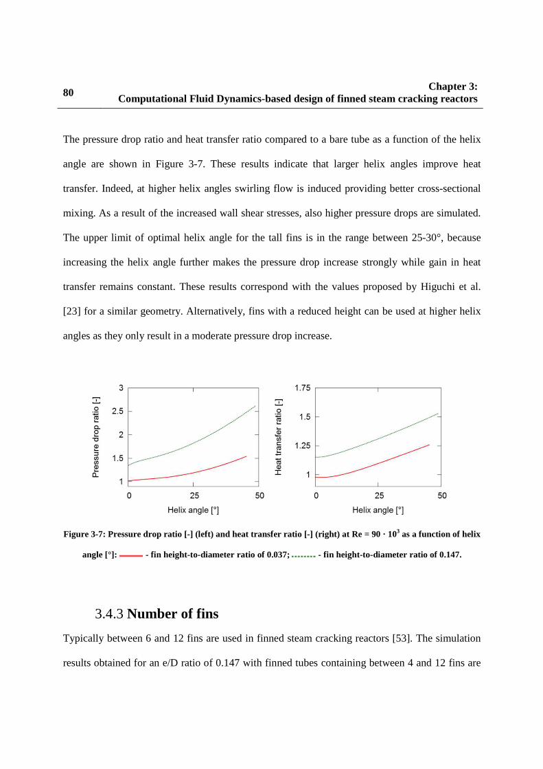
80 Chapter 3:
Computational Fluid Dynamics-based design of finned steam cracking reactors
The pressure drop ratio and heat transfer ratio compared to a bare tube as a function of the helix
angle are shown in Figure 3-7. These results indicate that larger helix angles improve heat
transfer. Indeed, at higher helix angles swirling flow is induced providing better cross-sectional
mixing. As a result of the increased wall shear stresses, also higher pressure drops are simulated.
The upper limit of optimal helix angle for the tall fins is in the range between 25-30°, because
increasing the helix angle further makes the pressure drop increase strongly while gain in heat
transfer remains constant. These results correspond with the values proposed by Higuchi et al.
[23] for a similar geometry. Alternatively, fins with a reduced height can be used at higher helix
angles as they only result in a moderate pressure drop increase.
Figure 3-7: Pressure drop ratio [-] (left) and heat transfer ratio [-] (right) at Re = 90 · 103 as a function of helix
angle [°]: - fin height-to-diameter ratio of 0.037; - fin height-to-diameter ratio of 0.147.
Number of fins 3.4.3
Typically between 6 and 12 fins are used in finned steam cracking reactors [53]. The simulation
results obtained for an e/D ratio of 0.147 with finned tubes containing between 4 and 12 fins are

Chapter 3: Computational Fluid Dynamics-based design of finned steam cracking reactors
81
shown in Figure 3-8. The tubes with 4, 6, 8, 10 and 12 fins have a wetted perimeter ratio of 1.11,
1.26, 1.44, 1.78 and 1.90 respectively. For the helicoidally finned tubes, the helix angle was again
15.88°. A linear relation between the number of fins and pressure drop is observed for both the
longitudinally finned and helicoidally finned tubes. However, the heat transfer ratio increases
only up to 8 to 10 fins. For tubes with more than 10 fins, it was seen that the flow inside the fin
valley gets isolated from the tube center leading to lower velocities. As soon as flow isolation
inside the fin occurs, an additional heat transfer resistance emerges due to the narrow passing
from the fin valley to the tube center. The simulations illustrate that the optimal number of fins
depends strongly on the chosen fin height, which in this case results in an optimal value of 8 to
10 fins. For fins with a small fin height-to-diameter ratio a higher number of fins can be adopted.
Figure 3-8: Pressure drop ratio [-] (left) and heat transfer ratio [-] (right) at Re = 90 103 as a function of
number of fins [-]: - longitudinally finned; - helicoidally finned.

82 Chapter 3:
Computational Fluid Dynamics-based design of finned steam cracking reactors
Geometry optimization 3.4.4
The parametric study assessed the performance of finned tubes for non-reactive air flow in terms
of pressure drop and heat transfer. It allows formulating several guidelines towards optimal steam
cracking reactor design. Ideally low pressure drops are combined with a high radial temperature
uniformity, giving rise to high light olefin selectivity and a reduced coking tendency [54]. Hence,
based on the results of the preceding parametric study, a design with a small fin height seems
potentially attractive because this allows to take maximal advantage of the lower pressure drops
these fins induce. In combination with a large value for the helix angle, this could lead to a large
increase in heat transfer by swirling flow for a low pressure drop increase. In any case, a clear
trade-off between heat transfer enhancement and additional pressure drop needs to be made. This
becomes clear from Figure 3-9, in which all simulation data points acquired throughout the
parametric study are plotted. The relationship between the relative heat transfer and relative
pressure drop is highly linear, but it is not obvious to assess the effect on product selectivities and
run length based on these data. Translating these guidelines to optimal fin height and number of
fins has allowed defining two optimal geometries that should significantly outperform the
previously studied tubes. The dimensions of these optimized designs are summarized in Table
3-2.

Chapter 3: Computational Fluid Dynamics-based design of finned steam cracking reactors
83
Table 3-2: Dimensions of optimal tube geometries.
Tube ID O1 O2 Inner diameter [10-3 m] 35.34 31.32 Fin height [10-3 m] 3.89 1.15 Number of fins [-] 10 24 Helix angle [°] 28.7 44.1 Wetted perimeter ratio [-] 1.367 1.212 U ratio [-] for inlet Reynolds number of 90 · 103/ 130 · 103 1.31 / 1.33 1.53 / 1.43 Pressure drop ratio [-] for inlet Reynolds number of 90 · 103 / 130 · 103 1.48 / 1.56 1.99 / 1.83
Geometry “O1” has fins with an e/D ratio of 0.11. The helix angle and number of fins were
chosen at the optimal values found in the parametric study for the taller fins, i.e. 8 to 10 fins and a
helix angle between 25° and 30°. For geometry “O2”, 24 small fins are combined with a high
helix angle. Both optimized geometries were found to offer increased heating characteristics as
seen in Figure 3-9. Mainly at the highest Reynolds number a better performance is simulated, i.e.
for a given pressure drop the heat transfer is higher.
Figure 3-9: Heat transfer ratio [-] as a function of pressure drop ratio [-] at Re = 90 · 103 (left) and 130 · 103
(right) for longitudinally finned; , helicoidally finned; and optimized geometries; .
84 Chapter 3:
Computational Fluid Dynamics-based design of finned steam cracking reactors
For application in steam cracking reactors, it can be concluded that the optimal geometry will be
largely dependent on the process conditions, i.e. mainly the Reynolds number. Furthermore a
trade-off between improved heat transfer and increased pressure drop must be made, which
depends on the applied feedstock as changes in product selectivity due to the higher pressure drop
will differ for different feedstocks [54]. Hence, non-reactive experiments and simulations can
offer guidelines for design, but reactive CFD simulations are necessary to assess the actual effect
on product yields and coking.
3.5 Reactive simulations of an industrial propane cracker
Reactive simulations of one of the reactors in an industrial Millisecond furnace were performed
to assess the effect of finned reactors on product yields and coking tendency. Millisecond
furnaces operate at very high severity and a residence time of approximately 0.1 seconds.
Millisecond furnaces are designed to achieve maximum ethene yield resulting in high operating
temperatures and very short run lengths, sometimes as short as one week.
Process conditions and reactor configurations 3.5.1
A 100 % pure propane feedstock was adopted. The hydrocarbon and steam flow rate were set to
0.03292 kg/s and 0.01075 kg/s respectively, resulting in a steam dilution 0.33. The reactor inlet
temperature was equal to 903.7 K while the reactor outlet pressure, i.e. just upstream the transfer
line exchanger, was set to be 170 kPa, i.e. the industrially applied value.

Chapter 3: Computational Fluid Dynamics-based design of finned steam cracking reactors
85
A coupled three-dimensional furnace-reactor simulation requires several iterations between the
reactor and furnace simulations and is at present difficult due to too high computational cost and
is considered outside of the scope of this work. Therefore a heat flux profile was set as boundary
condition on the outer wall of the reactor. This heat flux profile was taken from a furnace
simulation where the boundary condition applied to the outer wall of the reactor tubes was the
industrially measured outer wall temperature profile. The adopted models in the furnace
simulation were similar to those of Hu et al. [55].
Four different reactor configurations were simulated. Their dimensions are summarized in Table
3-3. First, a bare tube (Bare) was simulated as a reference case. Second, an industrially applied
helicoidally finned reactor (Helix) was considered. The fin dimensions of this reactor are close to
those of the optimized geometry “O1”, viz. Table 3-2, of the parametric study. Third, the same
fin parameters were applied in simulating a reactor with longitudinal fins (Straight). Finally, a
tube with significantly smaller fins was simulated (SmallFins) corresponding to the optimized
geometry “O2”.
Table 3-3: Reactor dimensions.
Reactor ID Bare Helix Straight SmallFins Reactor length [m] 10.556 10.556 10.556 10.556 Adiabatic inlet section [m] 0.444 0.444 0.444 0.444 Maximum inner diameter [10-3 m] 30.2 34.8 34.8 31.3 Number of fins [-] - 8 8 24 Helix angle [°] - 15.7 - 33.1 Outer diameter [10-3 m] 43.7 48.3 48.3 44.8 Metal thickness [10-3 m] 6.75 6.75 6.75 6.75 Fin height [10-3 m] - 4.8 4.8 1.15 Cross-sectional surface area [10-6 m²] 715.7 715.7 715.7 715.7 Cross-sectional perimeter [m] 0.0948 0.1315 0.1315 0.1150

86 Chapter 3:
Computational Fluid Dynamics-based design of finned steam cracking reactors
Results and discussion 3.5.2
The computational grid was constructed by extruding a 2D mesh of 1/8th of the cross section
applying the required twist vector for the helicoidally finned reactors. The grid size in wall units
was maintained at the values used throughout the parametric study which were confirmed to
provide grid-independent results, see Appendix B. This led to computational grids consisting of 6
to 11 million cells.
Computation was performed on 32-core Dell C6145 computing nodes with AMD Magny-Cours
Opteron 6136 processors and an Infiniband Double QDR communications link. Total CPU time
amounted to around 25000 hours per simulation, i.e. about one month of clock time. In the
following, many averaged variables are reported. The equations used to calculate the different
averages are given in Appendix C.
Figure 3-10 A and B show the mixing cup temperature and pressure as a function of the axial
position for the four reactor configurations. Little differences between the process gas
temperature profiles are simulated as the same heat input, reactor volume and mass flow rate are
adopted. However, the pressure drop varies drastically with SmallFins showing the highest
pressure drop. This higher pressure drop results in a higher inlet density yielding small
differences in residence time, calculated here as reactor volume divided by volumetric inlet flow
rate, as shown in Table 3-4.

Chapter 3: Computational Fluid Dynamics-based design of finned steam cracking reactors
87
Figure 3-10: Process gas temperature [K] (A) and pressure [kPa] (B) mixing cup averaged over a cross section
as a function of axial position [m]: - Bare; - Helix; - Straight ; -
SmallFins.

88 Chapter 3: Computational Fluid Dynamics-based design of finned steam cracking reactors
Figure 3-11 shows the azimuthally area-averaged external tube metal temperature as a function of
the axial position. The maximum external tube metal temperature occurs at around 3.5 m
corresponding to the maximum of the heat flux to the reactor. For the Bare reactor, the maximum
temperature is 1334 K, which is close to the maximum allowable TMT of 1363 K. This is caused
by the high cracking severity, i.e. the coil-outlet-temperature (COT) is above 1190 K. The
maximum TMT is 29, 26 and 51 K lower than the Bare reactor for Helix, Straight and SmallFins
respectively. For Millisecond furnaces the maximum tube metal temperature is typically the
limiting factor for the run length. Hence, decreasing this temperature by adopting finned tubes
will significantly increase the reactor run length.
Figure 3-11: Azimuthally area-averaged external tube metal temperature [K] as a function of axial position
[m]: - Bare; - Helix; - Straight; - SmallFins.

Chapter 3: Computational Fluid Dynamics-based design of finned steam cracking reactors
89
Table 3-4 summarizes the most important process conditions, product yields and selectivities. For
validation, data of an industrial bare tube Millisecond reactor running with a crude propane
feedstock, i.e. 95 % pure propane or higher, under similar, but not identical conditions have been
added. Considering the accuracy of the industrial yield measurements, the purity of the feed and
accounting for the fact that the industrial data are for a slightly lower cracking severity, the
agreement between the simulated Bare reactor and the industrial data is reasonable. Comparing
the four simulation cases some small differences in COT are observed. These can be attributed to
different reaction rates due to different pressure and temperature fields in the reactors. The coil-
inlet-pressure (CIP) increases drastically with a factor 1.22 and 1.39 for the Straight and Helix
reactor respectively. As expected from the parametric study, the SmallFins reactor shows the
highest pressure drop. The propane conversion is slightly higher for Helix and SmallFins, which
can be attributed to a higher space time due to the higher pressure drop. To limit the effect of
differences in propane conversion, comparison should be made on the basis of selectivities
expressed as product yield divided by propane conversion. As bimolecular reactions are favored
over monomolecular reactions at higher pressure, the selectivity to light olefins produced by
monomolecular beta scissions is reduced at higher reactor pressure. This effect can be clearly
seen in Table 3-4, where the ethene selectivity decreases monotonically with increasing pressure
drop ratio. The effect is limited as ethene selectivity only decreases by 0.56 wt%. However, given
the large scale of the steam cracking process, this difference is economically significant. The
selectivity to methane and 1,3-butadiene is increased as these are formed by a series of
bimolecular reaction steps.

90 Chapter 3:
Computational Fluid Dynamics-based design of finned steam cracking reactors
Surprisingly the SmallFins reactor has the highest propene selectivity although the conversion in
this reactor is higher than in all other reactors. Typically the propene yield decreases with
increasing conversion [56]. A rate of production analysis of the reaction mechanism reveals that
propene is primarily formed by C-H beta scissions of the 2-propyl radical while the addition
reaction of the hydrogen radical to propene results in the 1-propyl radical that further decomposes
to ethene and methyl:
(R1)
(R2)
As reported by Van Geem et al. [54] radial temperature gradients strongly affect the radical
concentrations and seem to be very likely responsible for the higher propene selectivity. To
further assess the effect of conversion on selectivities, a second simulation for the Bare reactor
configuration was performed at the same propane conversion of the SmallFins reactor. To this
end, the total heat input to the reactor was increased with 0.8 %. The results of this simulation are
summarized under Bare HighFlux in Table 3-4. Comparing these results with the SmallFins
simulation, it is clear that the reduced ethene selectivity for the SmallFins reactor is completely
balanced by the increased selectivity to propene and 1,3-butadiene as the total selectivity to
valuable light olefins is almost identical. Hence, application of optimal fin parameters does not
necessarily result in a loss of the total olefin selectivity and can be economically more attractive
for example during periods where propene and 1,3-butadiene are more valuable than ethene.

Chapter 3: Computational Fluid Dynamics-based design of finned steam cracking reactors
91
Table 3-4: Reactor conditions, product yields and selectivities for the four reactor configurations.
Bare Straight Helix SmallFins Bare HighFlux
Bare Industrial &
Coil-outlet-temperature [K] 1190.9 1191.2 1193.5 1192.7 1192.8 - Pressure drop [kPa] 29.13 35.68 40.49 48.42 28.92 - Pressure drop ratio [-] 1.00 1.22 1.39 1.66 0.99 - Propane conversion [-] 84.55 84.74 85.42 85.16 85.20 - P/E ratio [wt%/wt%] 0.476 0.471 0.471 0.485 0.467 0.50 Residence time [s] 0.149 0.154 0.157 0.163 0.149 -
Product Yields [wt%] H2 1.52 1.51 1.51 1.49 1.53 - CH4 18.75 19.03 19.22 19.25 18.88 19 C2H2 1.03 1.05 1.06 0.98 1.08 - C2H4 38.31 38.39 38.58 38.11 38.67 36 C2H6 3.65 3.59 3.58 3.46 3.69 3.5 C3H4 1.20 1.24 1.26 1.22 1.25 - C3H6 18.24 18.08 18.17 18.47 18.05 18 C3H8 15.45 15.26 14.58 14.84 14.80 17 1,3-C4H6 1.23 1.23 1.43 1.53 1.44 1.5 1-C4H8 0.54 0.53 0.54 0.56 0.54 - 2-C4H8 0.02 0.02 0.03 0.03 0.03 - n-C4H10 0.02 0.02 0.02 0.02 0.02 -
Valuable light olefins* 57.78 57.70 58.18 58.11 58.15 55
Product Selectivity [-] H2 1.80 1.78 1.77 1.75 1.80 - CH4 22.18 22.46 22.50 22.61 22.15 - C2H2 1.21 1.24 1.24 1.15 1.27 - C2H4 45.31 45.31 45.16 44.75 45.38 - C2H6 4.31 4.24 4.19 4.07 4.33 - C3H4 1.42 1.47 1.48 1.43 1.47 - C3H6 21.57 21.34 21.27 21.69 21.18 - 1,3-C4H6 1.46 1.45 1.67 1.79 1.69 - 1-C4H8 0.64 0.62 0.63 0.65 0.63 - 2-C4H8 0.03 0.03 0.03 0.03 0.03 - n-C4H10 0.02 0.02 0.02 0.02 0.02 -
Valuable light olefins* 68.34 68.10 68.10 68.24 68.25 - *Valuable light olefins is the sum of ethene, propene and 1,3-butadiene. & Detailed feed composition not available.

92 Chapter 3: Computational Fluid Dynamics-based design of finned steam cracking reactors
Figure 3-12 A shows the azimuthally mixing cup averaged process gas temperature as a function
of the radial position at an axial position of 10.5 m, i.e. near the reactor outlet. As the reactor
inner radii vary, the radial position is normalized. The Bare reactor has a temperature difference
between centerline and innerwall equal to 95.6 K. This value is in the same range as reported
previously by Van Geem et al. [54] using a 2D model and De Saegher et al. [53] using a 3D
model, although for different reactors and/or feedstocks. The temperature difference in
comparison with Bare is 13.3, 6.9 and 21.4 K lower for the Helix, Straight and SmallFins
respectively. Because of the lower inner wall temperatures, the finned reactors will yield lower
coking rates. The small maximum seen at 0.013 m for Helix and at 0.014 m for SmallFins is a
result of a zone with higher temperature in the wake of the fins as was also seen in Figure 3-4.
Figure 3-12 B shows the mixing cup propane yield as a function of the radial position at an axial
position of 10.5 m. The profiles are normalized to their respective value at the reactor centerline
to limit the effect of small differences in conversion. A relative difference of up to 10 % is
simulated between the center of the reactor and the reactor inner wall for the Bare reactor.
Surprisingly a larger difference of 18 % is observed for the Straight reactor. This is attributed to
the larger reactor maximum inner diameter compared to the Bare reactor and the absence of
enhanced mixing from swirling flow. The better mixing in the Helix reactor reduces the non-
uniformity although still not making up completely for the larger reactor inner diameter
compared to the Bare reactor. The SmallFins reactor benefits both from better mixing and a lower
tube diameter compared to Helix and Straight, yielding the most uniform profile. Figure 3-12 C
shows the mixing cup hydrogen radical yield as a function of radial position at an axial position
of 10.5 m. Again the values are normalized to their respective value at the reactor centerline to

Chapter 3: Computational Fluid Dynamics-based design of finned steam cracking reactors
93
limit the effect of small differences in conversion. Comparing these profiles with Figure 3-12 B,
it is clear that the hydrogen radical yield shows a much steeper profile close to the reactor wall
than the propane yield. This comparison holds for all radicals and molecules. The formation of
radicals through C-C and C-H scissions has a high activation energy, whereas the activation
energy of radical-consuming recombinations is close to zero. Hence, the formation of radicals is
favored at high temperatures. The ranking of radical uniformity between the reactors is therefore
equal to the ranking of temperature uniformity with Bare being the worst and Smallfins
performing best. Taking into account reactions R1 and R2 as determining the propene selectivity,
a higher hydrogen concentration near the wall will result in lower propene selectivity as reaction
R2 is favored over R1. Higher radial temperature uniformity results in a reduction of propene
consuming reactions, leading to a higher propene selectivity.

94 Chapter 3: Computational Fluid Dynamics-based design of finned steam cracking reactors
Figure 3-12: Azimuthally mixing cup averaged process gas temperature [K] (A), normalized propane yield
[wt%/wt%] (B) and normalized hydrogen radical yield [wt%/wt%] (C) as a function of radial position at an
axial position of 10.5 m: - Bare; - Helix; - Straight; - SmallFins.

Chapter 3: Computational Fluid Dynamics-based design of finned steam cracking reactors
95
As discussed in Chapter 1, coke formation during steam cracking of hydrocarbons is a complex
process. Three distinct mechanisms have been proposed [57]. First, there is a catalytic phase in
which the properties of the reactor alloy are important. Afterwards, a heterogeneous, non-
catalytic mechanism dominates. Coke can also be formed through a homogeneous non-catalytic
mechanism in which high-molecular polyaromatics condense, collide with the coke surface and
get incorporated in the coke layer. In steam cracking reactors, most coke is formed through the
heterogeneous, non-catalytic mechanism. The modeling of the coke formation is therefore
focused on this mechanism [58]. In this mechanism, radical active sites are formed on the coke
layer by abstraction reactions by gas-phase radicals followed by additions of gas phase olefins,
terminations by radicals, cyclizations and dehydrogenation [59]. Hence, the coking rate is
determined by the temperature and both molecular and radical gas-phase concentrations near the
gas-coke interface. As the time-scale for coke formation is much smaller than for gas-phase
reactions, a discrete approximation can be adopted. This means that coke formation can be
assumed constant in a certain time interval, typically 24 to 48 hours is sufficient [60, 61]. From
the performed simulations, the coking rate at start-of-run conditions, can thus be calculated in a
post-processing step from the species concentrations and inner wall temperature.
The semi-empirical coking model of Plehiers was used [60]. The parameters in this model were
fitted to experimental data using a one-dimensional plug flow reactor model and it has shown to
give reasonable agreement with both pilot and industrial coking rates [60]. The coking model of
Plehiers considers only ethene and propene as coke precursors. Given the typical species
concentrations in a propane cracker, these are indeed the main molecules adding to the active

96 Chapter 3: Computational Fluid Dynamics-based design of finned steam cracking reactors
radical sites on the coke layer. As the model kinetic parameters were fitted to experimental data
using a 1D model, the mixing cup ethene and propene concentrations are used. However, the
kinetic parameter estimation was performed for the coke-gas interface temperature. Hence, the
inner wall temperature is used here, rather than the mixing cup gas temperature.
Figure 3-13 shows the azimuthally area-averaged coking rate as a function of axial position for
the four reactor configurations. All profiles show two high values; the first around 6 m and the
second at the reactor outlet. This shape can be explained by considering the three contributions to
the coking rate, i.e. the inner wall temperature, the ethene concentration and the propene
concentration. The inner wall temperature shows a similar profile as the outer wall temperature
profile shown in Figure 3-11 having a maximum around an axial position of 4 m.
Figure 3-13: Azimuthally area-averaged coking rate [10-5 kg/m²/s] as a function of axial position [m]:
- Bare; - Helix; - Straight; - SmallFins.

Chapter 3: Computational Fluid Dynamics-based design of finned steam cracking reactors
97
The ethene and propene concentrations are depicted in Figure 3-14 A and B respectively. The
reactors with the highest pressure drop obviously show the highest concentrations due to a higher
gas density. The ethene concentration increases monotonically along the reactor. The propene
concentration has a maximum at 6 m. Hence, the maximum in coking rate at 6 m is a result of the
temperature and propene concentration maximum. The high value at the outlet results from the
high ethene concentration. Comparing SmallFins to Bare, coking rates are lowered by 48 % and
27 % at 6 m and 10 m respectively. Hence, run length can be extended greatly by application of
finned tubes as a given reduction in the coking rate results in a more than proportional increase of
the run length as shown by Wang et al. [62].

98 Chapter 3: Computational Fluid Dynamics-based design of finned steam cracking reactors
Figure 3-14: Ethene (A) and propene (B) concentration [mol/m³] mixing cup averaged over a cross section as a
function of axial position [m]: - Bare; - Helix; - Straight; - SmallFins.

Chapter 3: Computational Fluid Dynamics-based design of finned steam cracking reactors
99
Figure 3-15 A shows the coking rate as a function of the relative fin arc length. This relative fin
arc length is defined as the running arc length from one fin top to the next divided by the total arc
length of one fin. This normalization is necessary as the total fin arc length differs between
SmallFins on one side and Helix and Straight on the other. The shape is a direct result of the non-
uniform temperature at the reactor inner wall shown in Figure 3-15 B. The average inner wall
temperature is 17.2, 16.8 and 18.5 K lower than the temperature of the Bare reactor for the Helix,
Straight and SmallFins reactor respectively. The difference between minimum and maximum
temperature is about 15 K for Helix and Straight, whereas it is only 6 K for SmallFins. At a
relative fin arc length of 0.11, Helix shows a small bump. This is again caused by the higher
temperature in the wake of the fin also seen in Figure 3-4. The higher inner wall temperature in
the fin valley and resulting higher coke formation will lead to a reduction of the fin height by
coke filling up the fin valleys. This will be most pronounced for the Helix and Straight reactor as
coke in the fin valley grows about 30 % faster compared to the coke at the fin top. The more
uniform temperature profile for SmallFins results in a more uniform growth of the coke layer.
Here the difference in coking rate between fin top and valley is only 10%. Hence it is expected
that the increased heat transfer due to the finned structure will persist longer for SmallFins. The
large non-uniformity of the coking rate shows that azimuthally averaging the coking rate for run
length predictions of finned reactors as typically done for bare reactors in 1D and 2D reactor
models can severely bias the results. For future work it is therefore advised to take the non-
uniform buildup of coke over time into account in order to make realistic run length predictions.

100 Chapter 3: Computational Fluid Dynamics-based design of finned steam cracking reactors
Figure 3-15: Coking rate [10-5 kg/m²/s] (A) and inner wall temperature [K] (B) as a function of the relative fin
arc length (0: top; 0.5: valley; 1.0: top) at an axial position of 10.5 m: - Bare; - Helix;
- Straight; - SmallFins.

Chapter 3: Computational Fluid Dynamics-based design of finned steam cracking reactors
101
3.6 Conclusions A three-dimensional reactor model was used for the simulation of internally finned steam
cracking reactor tubes. The model agreed well with the experimental validation data of Albano et
al. [50] obtained with air. A parametric study optimizing the fin parameters, i.e. fin height, helix
angle and number of fins, to maximize heat transfer revealed that the application of small fins
with a large helix angle leads to an overall increase in heat transfer for a similar pressure drop.
Two optimized designs outperformed all other tube geometries of the parametric study regarding
heat transfer. These optimized designs were compared with conventionally used bare reactor
tubes for an industrial Millisecond furnace. The reactive simulations with a detailed free-radical
reaction mechanism of 203 reactions and 26 species showed that helicoidally finned tubes
performed better in comparison to longitudinally finned tubes. Mainly the configuration with 24
small fins and a high helix angle outperformed all other configurations in terms of heat transfer.
The corresponding coking rates were found to be 30-50 % lower than for the bare tube depending
on the fin parameters, which will lead to improved run lengths. However, the large non-
uniformity of the coking rates in the azimuthal coordinate could lead to local buildup of coke
over time and could affect the performance. The calculated pressure drop for the finned
geometries is significantly higher, especially for the helicoidally finned reactors. It was seen that
this can reduce the relative ethene selectivity by more than 1 %, while it increases selectivity to
propene and 1,3-butadiene. An economic trade-off for a specific unit, evaluating the effect of
longer run length and shift in light olefin selectivity, should determine the final decision of
application of finned reactors. The presented CFD simulations can provide data for such
evaluations.

102 Chapter 3: Computational Fluid Dynamics-based design of finned steam cracking reactors
References [1] T. Ren, M. Patel, K. Blok, Olefins from conventional and heavy feedstocks: Energy use in steam cracking and alternative processes, Energy, 31 (2006) 425-451. [2] K.M. Van Geem, G.B. Marin, N. Hedebouin, J. Grootjans, Energy efficiency of the cold train of an ethylene cracker, Oil Gas-Eur. Mag., 34 (2008) 95-99. [3] T. Ren, M.K. Patel, K. Blok, Steam cracking and methane to olefins: Energy use, CO2 emissions and production costs, Energy, 33 (2008) 817-833. [4] K.M. Van Geem, M.F. Reyniers, G.B. Marin, Two severity indices for scale-up of steam cracking coils, Industrial & Engineering Chemistry Research, 44 (2005) 3402-3411. [5] J. Wang, M.-F. Reyniers, G.B. Marin, Influence of dimethyl disulfide on coke formation during steam cracking of hydrocarbons, Industrial & Engineering Chemistry Research, 46 (2007) 4134-4148. [6] J. Wang, M.-F. Reyniers, K.M. Van Geem, G.B. Marin, Influence of silicon and silicon/sulfur-containing additives on coke formation during steam cracking of hydrocarbons, Industrial & Engineering Chemistry Research, 47 (2008) 1468-1482. [7] M.-F. Reyniers, G.F. Froment, Influence of metal-surface and sulfur addition on coke deposition in the thermal-cracking of hydrocarbons, Industrial & Engineering Chemistry Research, 34 (1995) 773-785. [8] S.B. Parks, C.M. Schillmoller, Use alloys to improve ethylene production, Hydrocarbon Processing, 75 (1996) 53-&. [9] P. Broutin, F. Ropital, M.-F. Reyniers, G.F. Froment, Anticoking coatings for high temperature petrochemical reactors, Oil & Gas Science and Technology - Revue D'Institut Français du Pétrole Energies Nouvelles, 54 (1999) 375-385. [10] T. Redmond, M.P. Bergeron, Tests demonstrate anticoking capability of new coating, Oil & Gas Journal, 97 (1999) 39-42. [11] S. Petrone, Y. Chen, R. Deuis, L. Benum, D. Gent, R. Saunders, C. Wong, Catalyzed-assisted Manufacture of Olefins (CAMOL): Realizing Novel Operational Benefits from Furnace Coil Surfaces, AIChE 2008 Spring National Meeting, New Orleans, Louisiana, 2008. [12] S. Petrone, R. Deuis, F. Kong, Y. Chen, Catalytic surfaces and coatings for the manufacture of petrochemicals, B. Corporation, (2013). [13] S. Petrone, R. Mandyam, A. Wysiekierski, Surface alloyed high temperature alloys, S.E.P. Corp., (1997). [14] S. Petrone, R. Manyam, A. Wysiekierski, K. Tzatzov, Y. Chen, A "carbon-like" coating to improved coking resistance in pyrolysis furnaces, 10th Annual Ethylene Producers' Conference, New Orleans, LA, 1998. [15] A. Ganser, K.A. Wynns, A. Kurlekar, Operational experience with diffusion coatings on steam cracker tubes, Materials and Corrosion-Werkstoffe Und Korrosion, 50 (1999) 700-705. [16] T.S. Ravigururajan, A.E. Bergles, Development and verification of general correlations for pressure drop and heat transfer in single-phase turbulent flow in enhanced tubes, Experimental Thermal and Fluid Science, 13 (1996) 55-70.

Chapter 3: Computational Fluid Dynamics-based design of finned steam cracking reactors
103
[17] M.K. Jensen, A. Vlakancic, Experimental investigation of turbulent heat transfer and fluid flow in internally finned tubes, International Journal of Heat and Mass Transfer, 42 (1999) 1343-1351. [18] G.J. Zdaniuk, L.M. Chamra, P.J. Mago, Experimental determination of heat transfer and friction in helically-finned tubes, Experimental Thermal and Fluid Science, 32 (2008) 15. [19] T.S. Ravigururajan, A.E. Bergles, Visualization of Flow Phenomena Near Enhanced Surfaces, Journal of Heat Transfer, 116 (1994) 54-57. [20] D.J. Brown, Internally finned radiant coils: a valuable tool for improving ethylene plant economics, 6th EMEA Petrochemicals Technology Conference, London, U.K., 2004. [21] J.V. Albano, K.M. Sundaram, M.J. Maddock, Applications of Extended Surfaces in Pyrolysis Coils, Energy Progress, 8 (1988) 160-168. [22] J.J. De Saegher, T. Detemmerman, G.F. Froment, Three dimensional simulation of high severity internally finned cracking coils for olefins production, Revue De L'Institut Français Du Pétrole, 51 (1996) 245-260. [23] J. Higuchi, K. Hamaogi, Metal Tube for Pyrolysis Reaction, (2009). [24] P. Wolpert, B. Ganser, D. Jakobi, R. Kirchheiner, Process and finned tube for the thermal cracking of hydrocarbons, US 2005/0131263 (2005) 18. [25] G.D. Stefanidis, B. Merci, G.J. Heynderickx, G.B. Marin, CFD simulations of steam cracking furnaces using detailed combustion mechanisms, Computers & Chemical Engineering, 30 (2006) 635-649. [26] G.D. Stefanidis, B. Merci, G.J. Heynderickx, G.B. Marin, Gray/nongray gas radiation modeling in steam cracker CFD calculations, Aiche Journal, 53 (2007) 1658-1669. [27] G.D. Stefanidis, K.M. Van Geem, G.J. Heynderickx, G.B. Marin, Evaluation of high-emissivity coatings in steam cracking furnaces using a non-grey gas radiation model, Chemical Engineering Journal 137 (2008) 411-421. [28] A. Habibi, B. Merci, G.J. Heynderickx, Impact of radiation models in CFD simulations of steam cracking furnaces, Computers & Chemical Engineering, 31 (2007) 1389-1406. [29] A. Habibi, B. Merci, G.J. Heynderickx, Multiscale modeling of turbulent combustion and NOx emission in steam crackers, Aiche Journal, 53 (2007) 2384-2398. [30] G. Hu, H. Wang, F. Qian, Numerical simulation on flow, combustion and heat transfer of ethylene cracking furnaces, Chemical Engineering Science, 66 (2011) 1600-1611. [31] G. Hu, H. Wang, F. Qian, K.M. Van Geem, C.M. Schietekat, G.B. Marin, Coupled simulation of an industrial naphtha cracking furnace equipped with long-flame and radiation burners, Computers & Chemical Engineering, 38 (2012) 24-34. [32] G.H. Hu, H.G. Wang, F. Qian, Y. Zhang, J.L. Li, K.M. Van Geem, G.B. Marin, Comprehensive CFD Simulation of Product Yields and Coking Rates for a Floor- and Wall-Fired Naphtha Cracking Furnace, Industrial & Engineering Chemistry Research, 50 (2011) 13672-13685. [33] Q. Tang, M. Denison, B. Adams, D. Brown, Towards comprehensive computational fluid dynamics modeling of pyrolysis furnaces with next generation low-NO(x) burners using finite-rate chemistry, Proceedings of the Combustion Institute, 32 (2009) 2649-2657. [34] X. Lan, J. Gao, C. Xu, H. Zhang, Numerical simulation of transfer and reaction processes in ethylene furnaces, Chemical Engineering Research & Design, 85 (2007) 1565-1579.

104 Chapter 3: Computational Fluid Dynamics-based design of finned steam cracking reactors
[35] M.K. Sabbe, K.M. Van Geem, M.-F. Reyniers, G.B. Marin, First Principle-Based Simulation of Ethane Steam Cracking, Aiche Journal, 57 (2011) 482-496. [36] W. Sun, M. Saeys, Construction of an Ab Initio Kinetic Model for Industrial Ethane Pyrolysis, Aiche Journal, 57 (2011) 2458-2471. [37] K.M. Van Geem, M.F. Reyniers, G.B. Marin, J. Song, W.H. Green, D.M. Matheu, Automatic reaction network generation using RMG for steam cracking of n-hexane, AIChE Journal, 52 (2006) 718-730. [38] E. Ranzi, A. Frassoldati, S. Granata, T. Faravelli, Wide-range kinetic modeling study of the pyrolysis, partial oxidation, and combustion of heavy n-alkanes, Industrial & Engineering Chemistry Research, 44 (2005) 5170-5183. [39] W.J. Pitz, C.J. Mueller, Recent progress in the development of diesel surrogate fuels, Progress in Energy and Combustion Science, 37 (2011) 330-350. [40] P.J. Clymans, G.F. Froment, Computer-generation of reaction paths and rate-equations in the thermal cracking of normal and branched paraffins, Computers & Chemical Engineering, 8 (1984) 137-142. [41] K.M. Van Geem, D. Hudebine, M.-F. Reyniers, F. Wahl, J.J. Verstraete, G.B. Marin, Molecular reconstruction of naphtha steam cracking feedstocks based on commercial indices, Computers & Chemical Engineering, 31 (2007) 1020-1034. [42] K.M. Van Geem, R. Zajdlik, M.-F. Reyniers, G.B. Marin, Dimensional analysis for scaling up and down steam cracking coils, Chemical Engineering Journal, 134 (2007) 3-10. [43] J.E. Jones, On the Determination of Molecular Fields. I. From the Variation of the Viscosity of a Gas with Temperature, Proceedings of the Royal Society of London. Series A, 106 (1924) 441-462. [44] R.B. Bird, W.E. Stewart, E.N. Lightfoot, Transport Phenomena, Wiley, 2006. [45] E.W. Lemmon, R.T. Jacobsen, Viscosity and Thermal Conductivity Equations for Nitrogen, Oxygen, Argon, and Air, International Journal of Thermophysics, 25 (2004) 21-69. [46] H.A. McGee, Molecular Engineering, McGraw-Hill, New York, 1991. [47] K.K.Y. Kuo, Principles of Combustion, Wiley-Interscience, New York, 2005. [48] B.P. Leonard, Order of accuracy of QUICK and related convection-diffusion schemes, Applied Mathematical Modelling, 19 (1995) 640-653. [49] B. Andersson, R. Andersson, L. Hakansson, M. Mortensen, R. Sudiyo, B. van Wachem, Computational Fluid Dynamics for Engineers, 7th ed., Cambridge University Press, 2012. [50] J.V. Albano, K.M. Sundaram, M.J. Maddock, Applications of extended surfaces in pyrolysis coils, Energy Progress, 8 (1988) 9. [51] T. Von Kármán, Mechanical similitude and turbulence, National Advisory Committee for Aeronautics, Washington D.C., 1931. [52] P. Wolpert, B. Ganser, D. Jakobi, R. Kirchheiner, Process and finned tube for the thermal cracking of hydrocarbons, (2005). [53] J.J. De Saegher, T. Detemmerman, G.F. Froment, Three dimensional simulation of high severity internally finned cracking coils for olefins production, Oil & Gas Science and Technology - Revue de l'Institut Francais du Petrole, 51 (1996) 245-260. [54] K.M. Van Geem, G.J. Heynderickx, G.B. Marin, Effect of radial temperature profiles on yields in steam cracking, AIChE Journal, 50 (2004) 173-183.

Chapter 3: Computational Fluid Dynamics-based design of finned steam cracking reactors
105
[55] G. Hu, H. Wang, Q. Feng, K.M. Van Geem, C.M. Schietekat, G.B. Marin, Coupled simulation of an industrial naphtha cracking furnace equipped with long-flame and radiation burners, Computers & Chemical Engineering, 38 (2012) 24-34. [56] G.F. Froment, Kinetics and reactor design in the thermal-cracking for olefins production, Chemical Engineering Science, 47 (1992) 2163-2177. [57] S. Wauters, G.B. Marin, Kinetic Modeling of Coke Formation during Steam Cracking, Industrial & Engineering Chemistry Research, 41 (2002) 2379-2391. [58] S. Wauters, G.B. Marin, Computer generation of a network of elementary steps for coke formation during the thermal cracking of hydrocarbons, Chemical Engineering Journal, 82 (2001) 267-279. [59] G.C. Reyniers, G.F. Froment, F.D. Kopinke, G. Zimmermann, Coke Formation in the Thermal Cracking of Hydrocarbons. 4. Modeling of Coke Formation in Naphtha Cracking, Industrial & Engineering Chemistry Research, 33 (1994) 2584-2590. [60] P.M. Plehiers, G.C. Reyniers, G.F. Froment, Simulation of the run length of an ethane cracking furnace, Industrial & Engineering Chemistry Research, 29 (1990) 636-641. [61] G.J. Heynderickx, G.F. Froment, Simulation and comparison of the run length of an ethane cracking furnace with reactor tubes of circular and elliptical cross sections, Industrial & Engineering Chemistry Research, 37 (1998) 914-922. [62] J.D. Wang, M.F. Reyniers, K.M. Van Geem, G.B. Marin, Influence of silicon and silicon/sulfur-containing additives on coke formation during steam cracking of hydrocarbons, Industrial & Engineering Chemistry Research, 47 (2008).

106 Chapter 3: Computational Fluid Dynamics-based design of finned steam cracking reactors
Chapter 4: Computational Fluid Dynamics simulations with detailed chemistry: Application of Pseudo-Steady State Approximation
107
Chapter 4:
Computational Fluid Dynamics simulations
with detailed chemistry: Application of
Pseudo-Steady State Approximation
This chapter has been submitted to Chemical Engineering Science Journal: Carl M. Schietekat, Kevin M. Van Geem, Guy B. Marin, Computational Fluid Dynamics simulations with detailed chemistry: Application of Pseudo-Steady State Approximation, submitted
108 Chapter 4:
Computational Fluid Dynamics simulations with detailed chemistry: Application of Pseudo-Steady State Approximation
Abstract Using detailed kinetic models in computational fluid dynamics (CFD) simulations is extremely
challenging because of the large number of species that are nowadays considered in these models
and the stiffness of the associated set of differential equations. A simplified 1D model does not
capture the required detail that reactor engineers need and leads to substantial differences
compared to the reference 3D simulations as is illustrated for propane steam cracking. A
methodology was developed to use detailed single-event microkinetic models in CFD simulations
of steam cracking reactors by on the fly application of the pseudo-steady state assumption on the
radicals. Depending on the reaction network size, a speedup factor from 7 to 54 was obtained
compared to the standard FLUENT routines. The yields of molecules matched those from the
standard routines well. For the concentration of the radicals near the reactor inner wall, there is an
average relative error of around 10 %. The methodology was then applied to the simulation of an
industrial propane cracking reactor. A conventional bare reactor and a helicoidally finned reactor
were compared. The adopted reaction network contained 85 species, of which 41 were radicals
and 44 were molecules. By application of the finned reactor, the maximum external tube
temperature is reduced by 44 K. The ethene selectivity is reduced by 0.17 % while propene and
1,3-butadiene selectivity increased by 0.08 and 0.03 % respectively. The benzene selectivity is
0.05 wt% higher in the helicoidally finned reactor because of the higher pressure drop.
Keywords: Computational fluid dynamics, detailed chemistry, pseudo-steady state
approximation, steam cracking, ethene, enhanced heat transfer

Chapter 4: Computational Fluid Dynamics simulations with detailed chemistry: Application of Pseudo-Steady State Approximation
109
4.1 Introduction Accurate simulation of reactive fluid flow requires first principles models for both the chemistry
and the fluid flow. For the former only comprehensive kinetic models consisting of elementary
reaction steps will yield accurate results over a wide range of conditions. In the field of
combustion, oxidation and pyrolysis, the fundamental modeling of gas-phase chemistry has
thrived over the last two decades driven by an improved knowledge of the reaction families, the
availability of rate coefficients [1] and the automation of kinetic model generation through
computer codes [2-10]. This increase in modeling accuracy is accompanied by a steep increase in
the size of kinetic models, with state of the art combustion and pyrolysis kinetic models easily
containing several hundred species and thousands of reactions [11-14] to account for all reaction
pathways and the intermediate species. Figure 4-1 displays the size of selected kinetic models for
thermal decomposition, oxidation and combustion processes over the last two decades. It is clear
that the number of species and reactions of the reaction networks has increased drastically.

110 Chapter 4:
Computational Fluid Dynamics simulations with detailed chemistry: Application of Pseudo-Steady State Approximation
Figure 4-1: Number of reactions [-] as a function of number of species [-] of selected reaction networks for
oxidation, pyrolysis and combustion (after Lu and Law [15]) over the last two decades.
Notwithstanding the developments in accurate chemistry modeling, the implementation of these
detailed kinetic models in computational fluid dynamics (CFD) simulations remains a daunting
task because of two specific characteristics of these kinetic models. First, the simulation time
increases drastically with increasing size of the kinetic model as each species adds an extra
continuity equation to the system to be integrated. Second, these kinetic models show a large
spread in time scales associated with species and reactions [16]. This spread originates from the
distinct difference in reactivity of radical and molecular species and from reactions in partial
equilibrium. These two characteristics of the kinetic models, large size and stiffness, render
multidimensional CFD simulations very CPU time-intensive and often beyond the capabilities of

Chapter 4: Computational Fluid Dynamics simulations with detailed chemistry: Application of Pseudo-Steady State Approximation
111
computers available in most research centers [17]. This has resulted in two main categories of
reactive flow simulations [17]. On the one hand, one-dimensional models using detailed kinetic
models are often used for the assessment of the accuracy of (automatically generated) kinetic
models and for the simulation of lab-scale setups or even for industrial reactors if simplification
of the fluid flow to one dimension is possible. On the other hand, advanced engineering tools
relying on CFD methods used for the design of industrially relevant geometries usually model the
chemistry rather approximately by a few reactions [18, 19]. Merging these two categories, i.e.
unification of detailed kinetic models and CFD simulations, would allow the more accurate
design and optimization of reactive flows. This challenge has been widely recognized in the
combustion engineering community [20] and several methods for reducing the computational
cost associated with detailed kinetic models have been proposed. These can be roughly divided
into three categories: kinetic model reduction methods, storage/retrieval-based methods and
adaptive chemistry methods. Model reduction decreases the number of reactions and/or species or
reduces the number of independent variables by application of e.g. the pseudo-steady state
assumption (PSSA) [21-25], partial equilibrium (PE) [26, 27], vertical and horizontal lumping
[28, 29], intrinsic low dimensional manifold (ILDM) [30], directed relation graph (DRG) [31]
and computational singular perturbation (CSP) [32]. Storage/retrieval methods are based on
tabulation strategies for the species rate of formation. In-situ adaptive tabulation (ISAT) [33] and
Piecewise reusable implementation of solution mapping (PRISM) [34] are two examples with the
former using Taylor series and the latter using polynomial regression to obtain rates of formation
based on tabulated points. Finally, adaptive chemistry methods use several reduced kinetic
models, each valid for a subset of space of the simulation [35-39]. As the kinetic models are

112 Chapter 4:
Computational Fluid Dynamics simulations with detailed chemistry: Application of Pseudo-Steady State Approximation
tailored to a more narrow range of thermochemical conditions, they are smaller and a significant
speedup can be obtained.
For the steam cracking of hydrocarbons, there is an interest in shifting from conventional one-
dimensional plug flow modeling towards more fundamental, multidimensional reactive flow
modeling. First, the heat flux from the furnace to the reactors causes a radial gradient in the
process gas temperature and this radial temperature profile produces radial concentration profiles.
In the plug flow reactor model the rate of formation of a species is calculated using the cross-
sectional mixing cup temperature and concentrations. This value is not equal to the mixing cup
average rate of formation, i.e. �������, �� ≠ ��,����, � . Hence, depending on the
magnitude of the radial gradient, an error in the predicted product yields is made. In addition
coke is formed on the inside of the reactor. The rate of coke formation depends -among other
variables- largely on the inner wall temperature and on the gas-phase concentrations near the
inner wall. In a one-dimensional reactor model, the inner wall temperature is obtained via
correlations for the Nusselt number for fully developed, turbulent pipe flow such as the
Gnielinski correlation [40]. These correlations target at non-reactive flows and application to
endothermic reactive flows results in an overprediction of the difference between the inner wall
and the mixing cup process gas temperature as shown by Sundaram and Froment [41]. Also the
mixing cup species concentrations are typically used in the calculation of the coking rate even
though it has been shown that the near-wall concentrations differ significantly from the mixing
cup concentrations, most certainly for radicals [42, 43]. Secondly, the plug flow reactor model
fails to account for azimuthal non-uniformities in the heat flux profile to the reactors, e.g. because

Chapter 4: Computational Fluid Dynamics simulations with detailed chemistry: Application of Pseudo-Steady State Approximation
113
of shadow effects in the furnace. Heynderickx and Froment [44] showed that these azimuthal heat
flux non-uniformities can cause an azimuthal variation of 50 K in temperature and a 100 %
azimuthal variation in coking rate, but did not quantify the effect on the product yields. Finally,
the plug flow reactor model fails to account for the complex flow pattern caused by emerging
three-dimensional reactor technologies [43, 45, 46] and return bends [19]. Reckoning these
shortcomings, several authors have simulated steam cracking reactors with two-dimensional [42,
47-49] and three-dimensional reactor models [19, 43, 50-52]. In most of these studies, a severely
reduced kinetic model was used because of extremely large simulation times and difficulties in
achieving a converged solution with a detailed kinetic model.
In the present work, steam cracking reactors are simulated using detailed kinetic models. To limit
computational time, the pseudo-steady state assumption is applied to the radicals both a-priori
and on the fly. First, the three-dimensional simulation results are compared to one-dimensional
plug flow results. To this end, the one-dimensional simulation program COILSIM1D was
extended to account for radial non-uniformities in temperature and radical concentrations. After
an overview of the 3D model, the methodology is validated and the speedup in CPU time is
quantified. Next, the application of an optimized finned reactor technology in an industrial steam
cracking unit is simulated and the effect of the reactor geometry on product yields in analyzed.

114 Chapter 4:
Computational Fluid Dynamics simulations with detailed chemistry: Application of Pseudo-Steady State Approximation
4.2 Numerical models
Governing equations 4.2.1
4.2.1.1 One-dimensional reactor model
Instead of performing CPU-intensive simulations with a three-dimensional reactor model, plug
flow reactor models are more routinely used to simulate steam cracking reactors. The common
method to account for the effect of three-dimensional reactor technologies on product yields and
maximum external tube metal temperatures is by multiplication of the friction factor and Nusselt
number by a factor derived from non-reactive experiments or simulations as e.g. reported by
Albano et al. [53] and Schietekat et al. [45]. COILSIM1D is such a 1D reactor model for steam
cracking reactors incorporating a single-event microkinetic model of more than 700 species [13].
The governing equations of COILSIM1D are:
����� � ���4 ���,� (4.1)
����� � �2����� ! "�#$%&'� ! &' �'�� (4.2)
(��)*+,-�./
����� � ���� 0�� ! ���� �4 ( #��123�./ ��∆5�� (4.3)
with �� � 6��3711 , �3711 calculated from the Colebrook equation [54] and 6� a user-supplied
correction factor to account for the increased pressure drop by application of a three-dimensional
reactor technology. For the simulations in paragraph 4.3.3, 6� was set to unity for the Bare tube

Chapter 4: Computational Fluid Dynamics simulations with detailed chemistry: Application of Pseudo-Steady State Approximation
115
while for the SmallFins tube 6� was set to 1.99. These values were obtained from the non-
reactive flow simulations of Chapter 3 [43].
COILSIM1D was extended to account for the influence of the radial temperature and β-radical
concentration profiles on product yields and heat transfer by calculating the mixing cup rate of
formation ���,� in equation (4.1) over the cross-sectional area at each axial grid point zi during
numerical integration of the ordinary differential equations (4.1), (4.2) and (4.3). The well-known
power law velocity profile for fully developed pipe flow proposed by Prandtl [55] is assumed:
'�#� � '89 :1 � 2#��� <//� (4.4)
where n is typically taken to be 7 resulting in the one-seventh law. From heat-momentum
similarity, the following radial temperature distribution is assumed:
�#� � �� ! �32� 21 � �� � :1 � 2#��� <//� (4.5)
Figure 4-2 shows a flow sheet of the adopted calculation procedure. At the first point of the axial
grid, i.e. i=0 in Figure 4-2, the average temperature �� is the reactor inlet temperature supplied
by the user and the inner wall temperature is calculated using the heat flux at this axial position:
0�� � ℎ��� � �� (4.6)
with 0�� the heat flux per inner wall surface area, ℎ � 6?ℎ3711, 6? a user-supplied correction
factor and ℎ3711 calculated from the Gnielinski correlation [40]. For the simulations in paragraph
4.3.3, 6? was set to unity for the Bare tube while for the SmallFins tube 6? was set to 1.53. These
values were obtained from the non-reactive flow simulations of Chapter 3

116 Chapter 4:
Computational Fluid Dynamics simulations with detailed chemistry: Application of Pseudo-Steady State Approximation
@' � ��8 ��B � 1000�D#1 ! 12.7 :��8</ �G HD#� IG � 1J (4.7)
Next, 32� 21 is calculated by calculating the mixing cup temperature from equation (4.5) and
setting it equal to the value of the reactor inlet temperature:
�� � K L8�#��#��MNOK L8�#��MNO (4.8)
Hence, the radial temperature profile of equation (4.5) is defined. From this profile, the mixing
cup rates of formation ���,� are calculated:
���,� � K &�#�'�#������#�, �#� �#PQRS�O K &�#�'�#��#PQRS�O (4.9)
By substitution of the ideal gas law and neglecting the radial variation of pressure and molecular
mass, equation (4.9) becomes:
���,� � K '�#������#�, �#� �#� �#PQRS�O K '�#��#� �#PQRS�O (4.10)
With this ���,�, the plug flow equations (4.1), (4.2) and (4.3) are integrated over ∆zi, the axial
length of the axial grid point zi. Hence, updated values for � and �� are available. From
equation (4.6), �� is updated. If the difference between the old and the updated value of �� is
smaller than the threshold value εT, set to 0.01%, convergence is reached in this axial grid point
and the simulation is proceeded to the next axial grid point. The converged �� and �� are used

Chapter 4: Computational Fluid Dynamics simulations with detailed chemistry: Application of Pseudo-Steady State Approximation
117
as initial guess for the next grid point. This procedure is repeated until the end of the reactor is
reached, i.e. zi = L.
Figure 4-2: Flow sheet of calculation procedure in COILSIM1D to account for radial profiles.

118 Chapter 4:
Computational Fluid Dynamics simulations with detailed chemistry: Application of Pseudo-Steady State Approximation
Three types of simulations were performed. First without taking into account any radial variation,
referred to as ‘1D’. Second, taking into account the radial temperature profile, referred to as ‘1D
T’, without accounting for radial variation in the species concentrations:
���,� � K '�#�����, �#� �#� �#PQRS�O K '�#��#� �#PQRS�O (4.11)
Finally, by taking into account both the radial temperature profile and the radial β-radials
concentration profile. The radial variation of the concentration of the molecules is neglected in all
simulations as it has been shown in Chapter 3 to be much smaller than the radial variation of the
β-radicals concentration [42, 43]. The β-radicals concentrations as a function of radial coordinate
are obtained by solving the algebraic equations resulting from application of the PSSA to the β-
radicals as a function of the radial coordinate:
��T+3 ��U, �V�#�, �#� � �T+� ��U, �V�#�, �#� (4.12)
Hence, equation (4.9) becomes:
���,� � K '�#��� H�U, �V�#�, �#�J�#� �#PQRS�O K '�#��#� �#PQRS�O (4.13)
4.2.1.2 Three-dimensional reactor model
The steady-state governing equations of a compressible, reactive, single-phase, fluid flow are
summarized in Table 4-1.

Chapter 4: Computational Fluid Dynamics simulations with detailed chemistry: Application of Pseudo-Steady State Approximation
119
Table 4-1: Continuity equations.
Total mass balance ∇ ∙ �&YZ� � 0 (4.14)
Navier-Stokes equations ∇ ∙ �&YZYZ� � �∇� ! ∇ ∙ [\ (4.15)
Process gas region energy equation ∇ ∙ �YZ�&] ! �� � ∇ ∙ ^_�,2��∇ �(ℎ� `b� c ! d? (4.16)
Reactor metal region energy equation
∇ ∙ �_e∇� � 0 (4.17)
Species continuity equation ∇ ∙ �YZ)� � �∇ ∙ `b ! �� , ∀h � 1, ij�B) � 1 (4.18)
In the gas-phase energy equation, ] � ℎ � *k ! |YZ|m� with the sensible enthalpy of the ideal gas
mixture calculated as ℎ � ∑ o�ℎ��e*23�./ and ℎ� � K pq���rrstu with p*,� defined as a temperature
polynomial with coefficients for the different species estimated with RMG’s
ThermoDataEstimator [5]. The effective conductivity of the process gas _�,2�� is the sum of the
laminar and turbulent thermal conductivity _�,2�� � _�,v ! _�, with _�,v calculated from kinetic
theory and _�, � 3wxSq1S with D# � 0.85 . `b is the diffusion flux of species h , including
contributions from both the laminar and turbulent diffusivity, i.e. b � � /zz+ H&{�,8 ! |S}3SJ ∇p� with d) � 0.7. Turbulent diffusion overwhelms laminar and thermal or Soret diffusion in steam
cracking reactors [43]. Hence, laminar diffusion is modeled rather approximate using kinetic
theory and Soret diffusion is neglected. The final term d? in the gas-phase energy equation is the
heat of reaction. For the metal tube, an energy equation is solved to account for conductive heat
transfer. The metal thermal conductivity _e is modeled as a temperature polynomial. �� is the rate

120 Chapter 4:
Computational Fluid Dynamics simulations with detailed chemistry: Application of Pseudo-Steady State Approximation
of formation of species h and ij�B) is the number of species. The k-ε RNG model was used for
the bare tubes while the Reynolds Stress Model was used for the helicoidally finned tube as it
showed better agreement to experimental data in Chapter 3 [43].
An adiabatic entrance zone with a length of 1.5 m was added upstream all reactors to ensure fully
developed velocity and turbulence parameters profiles at the reactor inlet. At the inlet boundary,
the process gas temperature, mass flow rate, turbulence parameters k and ε and the composition
of the process gas were imposed. The turbulence parameters were calculated for a turbulence
intensity of 8 % and a characteristic length scale of 10 % of the tube hydraulic diameter. At the
reactor outlet, a constant pressure boundary condition was set. The no-slip boundary condition
was set at the tube inner walls. The enhanced wall treatment was used to “bridge” the solution
variables in the near-wall cells. This model combines a two-layer model with enhanced wall
functions by blending linear and logarithmic laws-of-the-wall. Similar grids as in our previous
work were used, ensuring that the near-wall cells are within the viscous sub-layer, satisfying the
y+<1 condition [43]. A heat flux profile was applied to the reactor outer walls. The commercial
CFD code ANSYS FLUENT 13.0 was adopted to solve the governing equations.

Chapter 4: Computational Fluid Dynamics simulations with detailed chemistry: Application of Pseudo-Steady State Approximation
121
Calculation rate of production term 4.2.2
The calculation routine for the rate of production terms �� in the species continuity equations
(4.18) was tailored to steam cracking kinetics and implemented in a user-defined function (UDF).
4.2.2.1 Single-event microkinetic model
The adopted single-event microkinetic model was generated using the same methodology as
applied by Dijkmans et al. [56]. As the details of the methodology have been explained
previously [13, 56-58], only a brief summary of the key aspects is given here. The reaction
network consists of two parts: the β-network and the µ-network. The β-network contains the
reactions between molecules with less than 6 carbon atoms and radicals that can undergo only
bimolecular reactions or both mono- and bimolecular reactions, i.e. so-called β and βµ-radicals
respectively. The adopted β-network was obtained by reducing the β-network of Dijkmans et al.
[56] to the species relevant for propane cracking, the feedstock studied in this chapter. This
resulted in a β-network of 758 elementary reversible reactions between 42 molecules and 41
radicals. The β-network is appended with the µ-network, which is a collection of independent
sub-networks. In total, 31 sub-networks were included to account for the formation of aromatics.
In 15 sub-networks, a β(µ)-radical adds to an olefin to produce a C6+ radical. These radicals are
assumed to only undergo monomolecular reactions, i.e. the so-called µ-radical hypothesis.
Unsaturated µ-radicals can undergo ring closure reactions to form cyclic (di-)olefins. These
cyclic species can subsequently dehydrogenate to form aromatics via hydrogen abstractions, β-
scissions and C-H scissions which is described by the remaining 16 sub-networks. During

122 Chapter 4:
Computational Fluid Dynamics simulations with detailed chemistry: Application of Pseudo-Steady State Approximation
generation of a µ-network, the pseudo-steady state assumption is applied on the µ-radicals. In
combination with the µ-radical hypothesis, this results in a set of algebraic equations that can be
solved analytically to the µ-radicals’ concentrations. Hence, the concentration of each µ-radical
can be expressed as a function of the concentration of the starting species of the µ-network.
Substitution of these concentrations in the rate of formation terms makes the latter only
dependent on the concentrations of molecules and β(µ)-radicals. This not only reduces the
number of species continuity equations to be solved, but also greatly reduces the stiffness of the
set of differential equations. Consequently, the complete network contains 85 species, of which
41 radicals and 44 molecules. Validation of the reduced kinetic model for propane cracking was
performed by comparison to the full network of Dijkmans et al. [56] and is available in Appendix
A.
The thermodynamic data of the C4- molecules and β(µ)-radicals were derived from first principles
CBS-QB3 calculations of Sabbe et al. [59, 60]. Thermodynamic data of the µ-molecules was
estimated using RMG’s ThermoDataEstimator.
The Arrhenius parameters necessary to calculate the reaction rate coefficients are calculated
using a group additivity framework that is an extension of Benson’s group additivity [61-63]. The
reference parameters and group additive values used by Dijkmans et al. [56] were also adopted
here. Most are based on first principles calculations and none were fitted to experimental data. To
avoid time-consuming calculation of the reverse reaction rate coefficient by expressing
thermodynamic consistency during the fluid dynamics simulation, the reversible β-reactions were
split into two irreversible reactions by a-priori performing an linear regression of the reverse

Chapter 4: Computational Fluid Dynamics simulations with detailed chemistry: Application of Pseudo-Steady State Approximation
123
Arrhenius parameters to the values expressed by thermodynamic consistency in the relevant
temperature range, i.e. between 700 and 1300 K.
4.2.2.2 Pseudo-steady state assumption for β(µ)-radicals
Elimination of the µ-radicals by expressing the PSSA during network generation, greatly reduces
the number of species continuity equations and the system stiffness. However, the difference in
time scales between molecules and β-radicals is so large that significant stiffness still remains in
the system. This requires very strong under relaxation of the continuity equations of the β-
radicals to avoid divergence, making the simulation of industrial reactors computationally
impossible. Therefore the PSSA is applied to the β-radicals also. As the rate of formation of these
β-radicals contains terms that are second order in the PSS species, a-priori analytic calculation of
the β-radicals concentration as done for the µ-radicals is impossible. Lu and Law [64] developed
a method to obtain analytic solutions even when second order terms in the PSS species
concentrations are present. The nonlinear algebraic equations are first linearized and then
analytically solved with a directed graph. A good agreement was seen for the ignition delay time.
This methodology was not applied here as the nonlinear terms in the PSS equations are strongly
influenced by the higher pressure drop induced by three-dimensional reactor technologies and
contribute more than 10 % to the rate of consumption for some PSS species, such as methyl and
allyl radicals. Hence, to accurately model the effect of the reactor geometry on product yields,
accounting for these terms is necessary. Hence, the concentration of the β-radical ~� is calculated
numerically on the fly, i.e. during the flow simulations by expressing the rate for consumption
�T+3 to be equal to the rate of production �T+* :

124 Chapter 4:
Computational Fluid Dynamics simulations with detailed chemistry: Application of Pseudo-Steady State Approximation
��T+3 ��U, �V � �T+* ��U, �V (4.19)
Solving equation (4.19) numerically to �V can be unstable [64] while a robust solution method is
required as divergence of this algebraic solver would terminate the time-consuming flow
simulation. A tailored algebraic solver was used here that updates the concentration of the β-
radical j in iteration step n+1 via:
pT+��/ � pT+����T+*�T+3 � , i � 1. . i��o (4.20)
The concentration will increase if ��T+* � > ��T+3 � and decrease if the opposite holds. Convergence
is reached when ��T+* � � ��T+3 �, i.e. equation (4.19) expressing the PSSA for β-radical j holds. The
recursive relation is used until the relative change in concentration drops below a certain user-
specified threshold value ε for all PSS species or the maximum number of solver iteration steps
i��o is surpassed:
max∀� ��pT+��/ � pT+�pT+� �� < ��#i � i��o
A value of 1 % for the threshold value ε and 100 for the maximum number of iterations i��o
was found to be sufficient. In the first iteration steps of the flow solver, i��o is the limiting
factor. However, after several flow iterations, the PSS species concentration profiles change only
slightly and as the PSS concentrations of the previous iteration are taken as an initial guess for
pT+ , convergence is reached rapidly. Applying the PSSA to the β-radicals further reduces the
number of continuity equations to be integrated. As shown by Ren and Pope, the reactive system
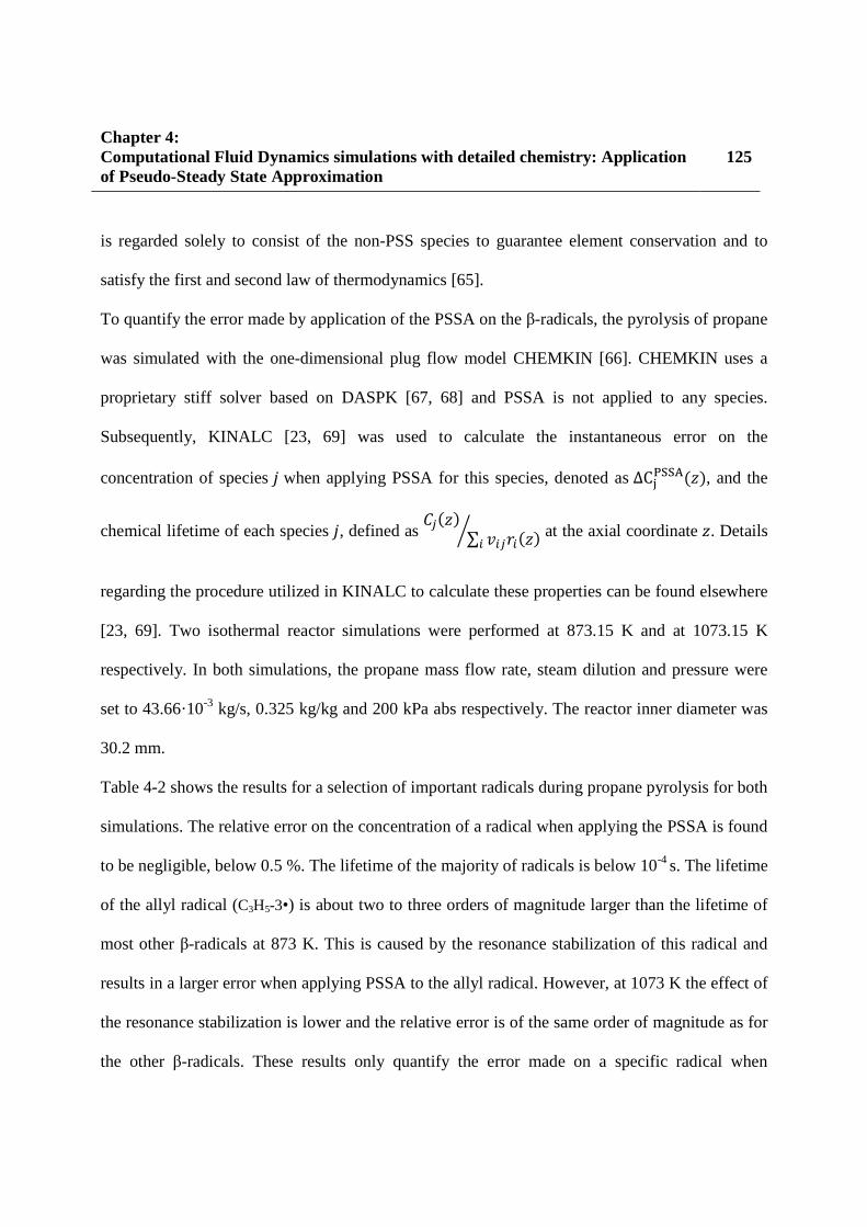
Chapter 4: Computational Fluid Dynamics simulations with detailed chemistry: Application of Pseudo-Steady State Approximation
125
is regarded solely to consist of the non-PSS species to guarantee element conservation and to
satisfy the first and second law of thermodynamics [65].
To quantify the error made by application of the PSSA on the β-radicals, the pyrolysis of propane
was simulated with the one-dimensional plug flow model CHEMKIN [66]. CHEMKIN uses a
proprietary stiff solver based on DASPK [67, 68] and PSSA is not applied to any species.
Subsequently, KINALC [23, 69] was used to calculate the instantaneous error on the
concentration of species h when applying PSSA for this species, denoted as ∆C��������, and the
chemical lifetime of each species h, defined as p���� ∑ ���#������ at the axial coordinate �. Details
regarding the procedure utilized in KINALC to calculate these properties can be found elsewhere
[23, 69]. Two isothermal reactor simulations were performed at 873.15 K and at 1073.15 K
respectively. In both simulations, the propane mass flow rate, steam dilution and pressure were
set to 43.66·10-3 kg/s, 0.325 kg/kg and 200 kPa abs respectively. The reactor inner diameter was
30.2 mm.
Table 4-2 shows the results for a selection of important radicals during propane pyrolysis for both
simulations. The relative error on the concentration of a radical when applying the PSSA is found
to be negligible, below 0.5 %. The lifetime of the majority of radicals is below 10-4 s. The lifetime
of the allyl radical (C3H5-3•) is about two to three orders of magnitude larger than the lifetime of
most other β-radicals at 873 K. This is caused by the resonance stabilization of this radical and
results in a larger error when applying PSSA to the allyl radical. However, at 1073 K the effect of
the resonance stabilization is lower and the relative error is of the same order of magnitude as for
the other β-radicals. These results only quantify the error made on a specific radical when
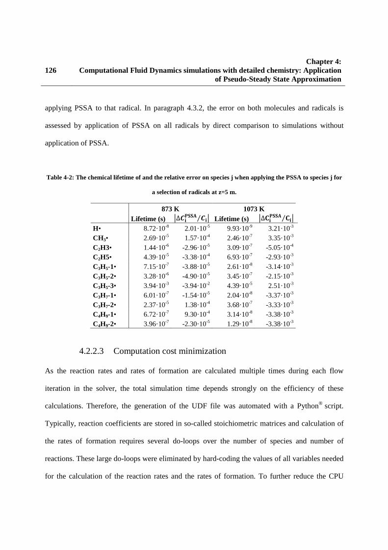
126 Chapter 4:
Computational Fluid Dynamics simulations with detailed chemistry: Application of Pseudo-Steady State Approximation
applying PSSA to that radical. In paragraph 4.3.2, the error on both molecules and radicals is
assessed by application of PSSA on all radicals by direct comparison to simulations without
application of PSSA.
Table 4-2: The chemical lifetime of and the relative error on species j when applying the PSSA to species j for
a selection of radicals at z=5 m.
873 K 1073 K
Lifetime (s) �∆������ ��⁄ � Lifetime (s) �∆������ ��⁄ � H• 8.72·10-8 2.01·10-5 9.93·10-9 3.21·10-3 CH3• 2.69·10-5 1.57·10-4 2.46·10-7 3.35·10-3 C2H3• 1.44·10-6 -2.96·10-5 3.09·10-7 -5.05·10-4 C2H5• 4.39·10-5 -3.38·10-4 6.93·10-7 -2.93·10-3 C3H5-1• 7.15·10-7 -3.88·10-5 2.61·10-8 -3.14·10-3 C3H5-2• 3.28·10-6 -4.90·10-5 3.45·10-7 -2.15·10-3 C3H5-3• 3.94·10-3 -3.94·10-2 4.39·10-5 2.51·10-3 C3H7-1• 6.01·10-7 -1.54·10-5 2.04·10-8 -3.37·10-3 C3H7-2• 2.37·10-5 1.38·10-4 3.68·10-7 -3.33·10-3 C4H9-1• 6.72·10-7 9.30·10-4 3.14·10-8 -3.38·10-3 C4H9-2• 3.96·10-7 -2.30·10-5 1.29·10-8 -3.38·10-3
4.2.2.3 Computation cost minimization
As the reaction rates and rates of formation are calculated multiple times during each flow
iteration in the solver, the total simulation time depends strongly on the efficiency of these
calculations. Therefore, the generation of the UDF file was automated with a Python® script.
Typically, reaction coefficients are stored in so-called stoichiometric matrices and calculation of
the rates of formation requires several do-loops over the number of species and number of
reactions. These large do-loops were eliminated by hard-coding the values of all variables needed
for the calculation of the reaction rates and the rates of formation. To further reduce the CPU

Chapter 4: Computational Fluid Dynamics simulations with detailed chemistry: Application of Pseudo-Steady State Approximation
127
time the calculations are processed using Maple®’s CodeGeneration package to generate an
optimal calculation procedure for the rates. This package detects common subexpressions,
calculates them once and stores them for subsequent use. An obvious example is to only calculate
the denominator 1/(RT) once and to store its value instead of calculating it again for every
reaction rate coefficient.
4.3 Results and discussion
One-dimensional vs. three-dimensional reactor model 4.3.1
In this section, the 3D simulation results of Chapter 3 [43] are compared to one-dimensional plug
flow simulation results to study the necessity of using a three-dimensional reactor model for
steam cracking reactors. As the PSSA was not applied in these 3D simulations, the plug flow
reactor model CHEMKIN was used [66]. The two reactor configurations referred to as Bare and
SmallFins reactor are discussed here. For both reactors, two one-dimensional simulations were
performed. In the first type of 1D simulations, referred to with ‘T’, the mixing cup temperature
profile from the corresponding 3D simulation is imposed. These simulations correspond to the
theoretical case where one would have perfect correlations for the friction and Nusselt numbers
resulting in perfect temperature and pressure profiles. In the second type of 1D simulation,
referred to with ‘Q’, the heat flux profile was applied to the reactor inner wall and scaled to
obtain the same conversion as in the corresponding 3D simulation. Both type of simulations use
the mixing cup pressure profile from the 3D simulations. Table 4-3 compares the 3D and the 1D
results and shows that in the 1D simulations with the imposed temperature profile, the conversion
is lower than in the corresponding 3D simulations. The difference is 2.57 wt% and 1.65 wt% for

128 Chapter 4:
Computational Fluid Dynamics simulations with detailed chemistry: Application of Pseudo-Steady State Approximation
the Bare and SmallFins reactor respectively. The higher conversion in the 3D simulations is
explained by accounting for the high temperature film near the reactor inner wall. As this high
temperature zone is less distinct in the SmallFins reactor, the agreement between the 1D and 3D
simulations is better. By matching the conversion, the total heat input is overpredicted by 1.07
and 2.59 % in the 1D simulations. This shows that when a coupled furnace-reactor simulation
[70, 71] is performed where the fuel flow rate to the furnace burners is adjusted to match a
desired cracking severity, e.g. conversion, the simulated fuel flow rate will be overestimated by
adopting a one-dimensional reactor model. Furthermore, the effect of the SmallFins reactor on
product selectivities compared to the Bare reactor is not well captured by the 1D simulations. For
ethene, the 1D simulations show a decrease in selectivity of 0.1 wt% while the 3D simulations
show a much larger decrease of 0.6 wt%. In contrast to the increase of 0.1 wt% in propene
selectivity simulated with the 3D model, a decrease of 0.2 wt% is seen from the 1D simulations.
Finally, the increase of 1,3-butadiene selectivity is underestimated; 0.1 wt% with the 1D
compared to 0.3 wt% with the 3D model. Although these differences are small, they are
significant to the economics of an industrial cracker. Hence, an accurate prediction of the effect
of a 3D reactor technology on product yields based on a 3D reactor model is necessary upon
evaluation of the installation of such a technology. Nonetheless, only detailed single-event
microkinetic models guarantee the desired accuracy. As stated above, the implementation of
these models in CFD simulations calls for CPU-time reducing methods such as the PSSA applied
here.

Chapter 4: Computational Fluid Dynamics simulations with detailed chemistry: Application of Pseudo-Steady State Approximation
129
Table 4-3: Comparison simulation results of three-dimensional simulations of Chapter 3 [43] and one-dimensional plug flow simulations with the 3D
mixing cup temperature and pressure profile (T,p) and with the 3D mixing cup pressure profile and heat flux profile scaled to the same conversion.
Bare_3D Bare_1D T, p Bare_1D Q, p SmallFins SmallFins_1D T, p SmallFins_1D Q, p
Coil-outlet-temperature [K] 1190.9 1190.9 1192.6 1192.7 1192.7 1192.6
Pressure drop [kPa] 29.13 29.13 29.13 48.42 48.42 48.42
Propane conversion [-] 84.55 81.99 84.55 85.16 83.50 85.16
Product Yields [wt%]
H2 1.52 1.43 1.47 1.49 1.44 1.47 CH4 18.75 18.13 18.90 19.25 18.69 19.21 C2H2 1.03 0.78 0.92 0.98 0.84 0.93 C2H4 38.31 35.89 37.45 38.11 36.66 37.66 C2H6 3.65 3.21 3.34 3.46 3.28 3.35 C3H4 (PD) 1.20 1.01 1.16 1.22 1.08 1.19 C3H6 18.24 19.01 18.56 18.47 18.85 18.52 C3H8 15.45 18.01 15.45 14.84 16.50 14.84 1,3-C4H6 1.23 1.79 2.06 1.53 1.95 2.14 1-C4H8 0.54 0.62 0.59 0.56 0.61 0.59 2-C4H8 0.02 0.04 0.04 0.03 0.04 0.04 n-C4H10 0.02 0.02 0.02 0.02 0.02 0.02 Product Selectivity [wt%] H2 1.80 1.75 1.74 1.75 1.73 1.72 CH4 22.18 22.11 22.35 22.61 22.38 22.56 C2H2 1.21 0.96 1.09 1.15 1.00 1.09 C2H4 45.31 43.78 44.29 44.75 43.90 44.23 C2H6 4.31 3.92 3.95 4.07 3.92 3.94 C3H4 (PD) 1.42 1.23 1.37 1.43 1.30 1.39

130 Chapter 4:
Computational Fluid Dynamics simulations with detailed chemistry: Application of Pseudo-Steady State Approximation
C3H6 21.57 23.19 21.95 21.69 22.57 21.75 C3H8 1.46 2.19 2.43 1.79 2.33 2.51 1,3-C4H6 0.64 0.76 0.70 0.65 0.73 0.69 1-C4H8 0.03 0.04 0.04 0.03 0.05 0.05 2-C4H8 0.02 0.02 0.02 0.02 0.02 0.02 Valuable olefinsa 68.34 69.15 68.67 68.24 68.81 68.49
a Valuable light olefins is defined as the sum of ethene, propene and 1,3-butadiene.

Chapter 4: Computational Fluid Dynamics simulations with detailed chemistry: Application of Pseudo-Steady State Approximation
131
Validation and speedup 4.3.2
To validate the application of the PSSA on the β-radicals and to quantify the obtained speedup,
three cases with different β-networks were studied. For all cases, a simulation was performed
with the developed UDF and with the standard FLUENT routines for calculating the rates of
formation. Simulations were performed for a bare tube on a 2D grid of 280,000 cells. An external
tube wall temperature profile was imposed on the reactor outer wall. The simulated reactor had a
length of 10 m, an internal diameter of 0.032 m and a wall thickness of 6 mm. The mass flow rate
was set to 0.01 kg/s and the inlet temperature to 873.15 K. The details of the used reaction
networks and the obtained speedup factor by application of the developed UDF compared to the
standard FLUENT routines are shown in Table 4-4.
Table 4-4: Specifications of the reaction networks and the obtained speedup factor in the 3D validation
simulations.
Feedstock Nr molecules Nr radicals Nr reactions Speedup factor Ethane 6 3 9 7.4 Butane 8 6 57 51.8
Propane 13 11 100 54.2
The speedup factor is seen to increase with the network size up to a speedup factor around 50.
The reason for the large speedup factor is threefold. Firstly, less continuity equations are to be
solved by application of PSSA on the radicals. Secondly, the calculation of the reaction rates and
rates of formation is optimized. Finally, the stiffness of the system is reduced. To avoid
divergence without application of PSSA, under-relaxation factors of 0.001 on the continuity

132 Chapter 4:
Computational Fluid Dynamics simulations with detailed chemistry: Application of Pseudo-Steady State Approximation
equations of the radicals were necessary. By application of PSSA, the under-relaxation factors of
all species continuity equations can be set to 0.9.
Figure 4-3 shows the mixing cup yields of the most abundant molecules as a function of the axial
coordinate in the Butane case. A good agreement between the PSSA and non-PSSA cases is seen
for all molecules. Figure 4-4 shows the mixing cup yields of several radicals as a function of the
axial coordinate in the Butane case. Some differences are seen here. Most notably, the radicals
that can be formed directly from the feedstock molecule butane have a non-zero value at the
reactor inlet which is most clearly seen for the methyl and ethyl radical. In general a small
underestimation is seen towards the end of the reactor as most clearly seen for the methyl radical.
Nonetheless the agreement is satisfactory.
Figure 4-3: Yields of molecules and butane conversion as a function of axial coordinate [m] in 3D validation
simulation ‘Butane’: symbols without PSSA; - butane conversion; - propene; - methane; - ethene;
- hydrogen; - ethane; full lines with PSSA.

Chapter 4: Computational Fluid Dynamics simulations with detailed chemistry: Application of Pseudo-Steady State Approximation
133
Figure 4-4: Yields of radicals as a function of axial coordinate [m] in 3D validation simulation ‘Butane’; -
methyl; - ethyl; - 1-butyl; - 2-butyl; - hydrogen radical; - allyl; full lines with PSSA.
As the species concentrations vary significantly from the reactor centerline to the reactor inner
wall [43] and as the concentrations near the wall are important for an accurate calculation of the
coke formation rate when using a fundamental coke formation model [42, 72, 73], the
concentrations in the Butane case as a function of radial coordinate at an axial position of 9.5 m
are compared in Figure 4-5 and Figure 4-6 for molecules and radicals respectively. When
applying PSSA on the β-radicals, the conversion near the reactor inner wall at an axial coordinate
of 9.5 m is 0.27 wt% higher than in the non-PSSA case. Consequently, the yield of the different
products is also slightly higher. A good agreement between the PSSA and non-PSSA case is seen
for the radical concentrations at the center of the reactor. Near the reactor inner wall, the radical
concentrations are overpredicted by applying the PSSA. The average relative error is about 10 %.
For the most important radical coke precursors, i.e. hydrogen, methyl and ethyl, the relative error
is 9, 15 and 9 % respectively. In the fundamental coking model of Wauters and Marin [72, 73],
an increase of the concentration of these radicals by 90 %, resulted in an increase of the coking

134 Chapter 4:
Computational Fluid Dynamics simulations with detailed chemistry: Application of Pseudo-Steady State Approximation
rate by about 640, 165 and 10 % respectively. Hence, it is clear that the error made on the radical
concentrations near the wall by application of PSSA is small but can have a significant influence
on the simulated coking rates.
Figure 4-5: Yields of molecules and butane conversion as a function of radial coordinate [·10-3 m] at an axial
position of 9.5 m in 3D validation simulation ‘Butane’: symbols without PSSA; - butane conversion; -
propene; - methane; - ethene; - hydrogen; - ethane; full lines with PSSA.
Figure 4-6: Yields of radicals as a function of radial coordinate [·10-3 m] at an axial position of 9.5 m in 3D
validation simulation ‘Butane’: symbols without PSSA; - methyl; - ethyl; - 1-butyl; - 2-butyl; -
hydrogen radical; - allyl; full lines with PSSA.

Chapter 4: Computational Fluid Dynamics simulations with detailed chemistry: Application of Pseudo-Steady State Approximation
135
Simulation of an industrial propane-cracking reactor 4.3.3
An industrial propane cracking reactor was simulated. The reactor is of the Millisecond type, i.e.
a straight tube with rather small length and diameter compared to other reactor designs. The
reactor length is 10.55 m and the tube cross-sectional flow area is 715.72 mm². A pure propane
feedstock is assumed. The dilution is 0.325 and the inlet temperature is 903.7 K. The outlet
pressure is 205.7 kPa abs. A heat flux profile as a function of axial coordinate is applied to the
reactor outer wall. The total heat input is 102.7 kW per reactor. A conventional bare reactor
(Bare) is compared to the optimized finned reactor ‘SmallFins’ of Chapter 3. The reactor details
are given in Chapter 3. As in Chapter 3, the cross-sectional flow area, reactor length, flow rate
and heat input are the same for the two simulations [43].
4.3.3.1 Discussion of three-dimensional simulation results
Figure 4-7 shows the external and internal tube metal temperature as a function of axial
coordinate. Maximum values occur where the heat flux to the reactor is maximal. The maximum
external tube temperature is 44 K lower in the SmallFins case compared to the Bare case.
Obviously, this will result in a significant increase of the run length. Table 4-5 shows the 3D
simulation results in the columns denoted with ‘Bare 3D’ and ‘SmallFins 3D’.

136 Chapter 4:
Computational Fluid Dynamics simulations with detailed chemistry: Application of Pseudo-Steady State Approximation
Figure 4-7: External and internal wall temperature [K] as a function of axial coordinate [m] in the 3D
simulations of the industrial propane-cracking reactor: - Bare external wall temperature; -
Bare internal wall temperature: - SmallFins external wall temperature; - SmallFins internal
wall temperature.
Figure 4-8 shows the azimuthally averaged mixing cup process gas temperature as a function of
the radial coordinate at an axial coordinate of 10.5 m for the two reactors. The temperature
difference between center and inner wall is 91 K for the Bare reactor. This is reduced to 65 K by
application of the SmallFins reactor. A small bump is seen at a radial coordinate of 15 mm for the
SmallFins reactor which can be attributed to the higher temperature in the wake of the fins [43].

Chapter 4: Computational Fluid Dynamics simulations with detailed chemistry: Application of Pseudo-Steady State Approximation
137
Figure 4-8: Azimuthally averaged mixing cup process gas temperature [K] as a function of the radial
coordinate at an axial coordinate of 10.5 m in the 3D simulations of the industrial propane-cracking reactor:
- Bare; - SmallFins.
Two phenomena influence the product selectivities in the SmallFins reactor compared to the Bare
reactor: the larger reactor pressure drop and the more uniform cross-sectional temperature profile.
Depending on the reaction path through which a certain product is formed, the former or the latter
might have a decisive influence. The less uniform cross-sectional temperature profile in the Bare
reactor will enhance the rate of reactions with a high activation energy. On the other hand, the
higher reactor pressure drop in the SmallFins will favor bimolecular over monomolecular
reactions.
For the same heat input, the conversion is 0.44 wt% higher in the SmallFins reactor than in the
Bare reactor. The mixing cup averaged propane conversion as a function of axial coordinate is

138 Chapter 4:
Computational Fluid Dynamics simulations with detailed chemistry: Application of Pseudo-Steady State Approximation
shown in Figure 4-9. The conversion initially increases faster in the Bare reactor as the induction
period for heating of the process gas is shorter. Indeed, the high temperature zone near the reactor
inner wall already induces C-C scissions more upstream resulting in the formation of radicals to
start reactions as shown in the insert of Figure 4-9. Further downstream the reactor, the mixing
cup averaged temperature profile of the two reactors is very similar and the higher pressure in the
SmallFins reactor results in higher reaction rates explaining the higher conversion in the
SmallFins reactor.
Figure 4-9: Mixing cup averaged propane conversion [%] as a function of axial coordinate [m] in the 3D
simulations of the industrial propane-cracking reactor: - Bare; - SmallFins.
As seen from Table 4-5, the selectivity towards methane is higher in the SmallFins reactor.
Methane is mainly formed by hydrogen abstractions on propane by the methyl radical. Van Geem

Chapter 4: Computational Fluid Dynamics simulations with detailed chemistry: Application of Pseudo-Steady State Approximation
139
et al. [42] simulated a higher methane yield using a two-dimensional simulation model compared
to a one-dimensional simulation model during cracking of ethane. This was attributed to the
higher concentration of the methyl radical because of the high temperature zone near the reactor
inner wall in the 2D model. Following this reasoning, a higher methane selectivity would be
expected in the Bare reactor. During cracking of ethane, the methyl radical is formed by C-C
scission of ethane, which has a high activation energy, i.e. about 377 kJ/mol [74]. However,
during cracking of propane, methyl is mainly formed by β-scission of the 1-propyl radical. This
reaction has a much lower activation energy (137 kJ/mol) and hence, a negligible difference in
mixing cup average concentration of the methyl radical is simulated. As formation of methane
from methyl mainly proceeds via bimolecular abstraction, the higher pressure drop in the
SmallFins reactor causes the higher methane selectivity.
Ea
= 377 kJ/mol (R4.1)
Ea = 137 kJ/mol (R4.2)

140 Chapter 4:
Computational Fluid Dynamics simulations with detailed chemistry: Application of Pseudo-Steady State Approximation
Table 4-5: Comparison simulation results for Bare and SmallFins reactor using a 3D model and the one-dimensional models 1D, 1D T and 1D T, β.
Bare 3D Bare 1D Bare 1D T Bare 1D T, β SmallFins 3D SmallFins 1D SmallFins 1D T SmallFins 1D T, β
Coil-outlet-temperature [K] 1168 1170 1169 1166 1167 1171 1170 1169
Heat input [kW] 102.7 104.3 103.2 103.1 102.7 104.0 103.4 103.2
Pressure drop [kPa] 23.0 25.5 25.5 25.6 45.6 45.1 45.0 45.6
P/E ratio [wt%/wt%] 0.70 0.73 0.73 0.73 0.71 0.72 0.72 0.72
Propane conversion [-] 75.1 75.1 75.1 75.1 75.6 75.6 75.6 75.6
Product Yields [wt%]
C4- 93.52 93.72 93.72 93.68 93.50 93.59 93.62 93.58
[C5+-Benzene[ 2.68 2.62 2.62 2.63 2.69 2.64 2.64 2.64
[Benzene-Naphthalene] 3.80 3.66 3.66 3.69 3.80 3.77 3.74 3.78
H2 2.05 2.04 2.04 2.04 2.05 2.04 2.03 2.05
CH4 15.00 15.10 15.10 15.10 15.22 15.32 15.32 15.32
C2H2 0.71 0.65 0.65 0.66 0.69 0.66 0.65 0.67
C2H4 27.26 26.86 26.86 26.89 27.29 27.10 27.10 27.12
C2H6 1.19 1.12 1.12 1.13 1.17 1.16 1.17 1.14
C3H4 0.82 0.79 0.79 0.80 0.80 0.79 0.78 0.80
C3H6 19.13 19.72 19.72 19.68 19.30 19.61 19.61 19.58
C3H8 24.85 24.91 24.91 24.87 24.41 24.38 24.41 24.39
1,3-C4H6 1.42 1.39 1.39 1.38 1.45 1.40 1.41 1.39
1-C4H8 0.89 0.94 0.94 0.93 0.93 0.93 0.94 0.93
2-C4H8 0.12 0.13 0.13 0.13 0.13 0.13 0.13 0.13
i-C4H8 0.06 0.07 0.07 0.07 0.07 0.07 0.07 0.07
n-C4H10 0.01 0.01 0.01 0.01 0.01 0.01 0.01 0.01
1,3-Cyclopentadiene 1.64 1.58 1.58 1.59 1.61 1.59 1.58 1.60
Me-1,3-Cyclopentadiene 0.36 0.35 0.35 0.35 0.36 0.35 0.34 0.34

Chapter 4: Computational Fluid Dynamics simulations with detailed chemistry: Application of Pseudo-Steady State Approximation
141
Benzene 2.43 2.46 2.46 2.48 2.48 2.53 2.51 2.54
Toluene 0.41 0.35 0.35 0.35 0.39 0.36 0.36 0.36
Styrene 0.10 0.08 0.08 0.08 0.10 0.08 0.08 0.09
Naphthalene 0.85 0.77 0.77 0.77 0.84 0.80 0.79 0.80
Product Selectivity [wt%]
C4- 91.37 91.64 91.64 91.59 91.52 91.56 91.51 91.37
[C5+-Benzene[ 3.57 3.49 3.50 3.50 3.50 3.49 3.49 3.57
[Benzene-Naphthalene] 5.06 4.91 4.98 4.95 4.98 4.95 5.00 5.06
H2 2.73 2.71 2.71 2.72 2.71 2.70 2.69 2.70
CH4 19.96 20.11 20.11 20.10 20.14 20.26 20.26 20.26
C2H2 0.94 0.87 0.87 0.88 0.91 0.87 0.86 0.89
C2H4 36.27 35.76 35.76 35.79 36.10 35.83 35.86 35.86
C2H6 1.58 1.49 1.49 1.50 1.55 1.53 1.54 1.51
C3H4 1.09 1.05 1.05 1.06 1.06 1.04 1.04 1.06
C3H6 25.45 26.26 26.26 26.20 25.53 25.93 25.94 25.90
1,3-C4H6 1.88 1.85 1.85 1.83 1.91 1.85 1.86 1.83
1-C4H8 1.19 1.25 1.25 1.24 1.23 1.23 1.24 1.23
2-C4H8 0.16 0.17 0.17 0.17 0.17 0.17 0.17 0.17
i-C4H8 0.09 0.09 0.09 0.09 0.09 0.09 0.09 0.09
n-C4H10 0.01 0.01 0.01 0.01 0.01 0.01 0.01 0.01
1,3-Cyclopentadiene 2.18 2.10 2.10 2.11 2.13 2.11 2.09 2.12
Me-1,3-Cyclopentadiene 0.48 0.46 0.46 0.46 0.48 0.46 0.46 0.45
Benzene 3.24 3.27 3.27 3.30 3.28 3.34 3.32 3.36
Toluene 0.55 0.46 0.46 0.47 0.52 0.47 0.47 0.48
Styrene 0.14 0.11 0.11 0.11 0.13 0.11 0.11 0.11
Naphthalene 1.13 1.02 1.02 1.03 1.11 1.05 1.05 1.05

142 Chapter 4:
Computational Fluid Dynamics simulations with detailed chemistry: Application of Pseudo-Steady State Approximation
The selectivity towards ethane is lower in the SmallFins reactor than in the Bare reactor. Ethane
is mainly formed by hydrogen abstraction by the ethyl radical and by recombination of two
methyl radicals. Figure 4-10 shows the rate of formation of ethane by these two contributions.
The methyl recombination is bimolecular and hence is favored at higher pressure. The
concentration of the ethyl radical in the Bare reactor is higher than in the SmallFins reactors
because of the high temperature zone near the reactor inner wall. Ethyl radicals are mainly
formed via C-C scission of propane having a high activation energy, i.e. about 370 kJ/mol [74].
As the lion’s share of the ethane formation goes through ethyl radicals as shown in Figure 4-10,
the higher ethane formation via the ethyl radical in the Bare reactor compensates the high
pressure effect on the bimolecular recombination reaction in the SmallFins reactor.
(R4.3)
(R4.4)

Chapter 4: Computational Fluid Dynamics simulations with detailed chemistry: Application of Pseudo-Steady State Approximation
143
Figure 4-10: Rate of formation [mol/m³/s] of ethane as a function of axial coordinate [m]: - by ethyl
hydrogen abstraction; - by methyl-methyl recombination.
A lower ethene selectivity is simulated by application of the SmallFins reactor compared to the
Bare reactor. Ethene is mainly formed by the β-scission of the 1-propyl radical. This 1-propyl
radical is formed by hydrogen addition to propene. As shown in Figure 4-11, the hydrogen
radical yield is higher in the Bare than in the SmallFins reactor. This higher hydrogen radical
yield results in a higher rate of formation of 1-propyl and subsequently a higher ethene
production. As this pathway consumes propene, it also explains the higher propene selectivity in
the SmallFins reactor.

144 Chapter 4:
Computational Fluid Dynamics simulations with detailed chemistry: Application of Pseudo-Steady State Approximation
Figure 4-11: Hydrogen radical yield [10-7 wt%] as a function of axial coordinate [m] in the 3D simulations of
the industrial propane-cracking reactor: - Bare; - SmallFins.
A slightly higher selectivity towards 1,3-butadiene, 1-butene and 2-butene is simulated. Figure
4-12 shows a scheme of the most important reactions leading to the formation of these
components.
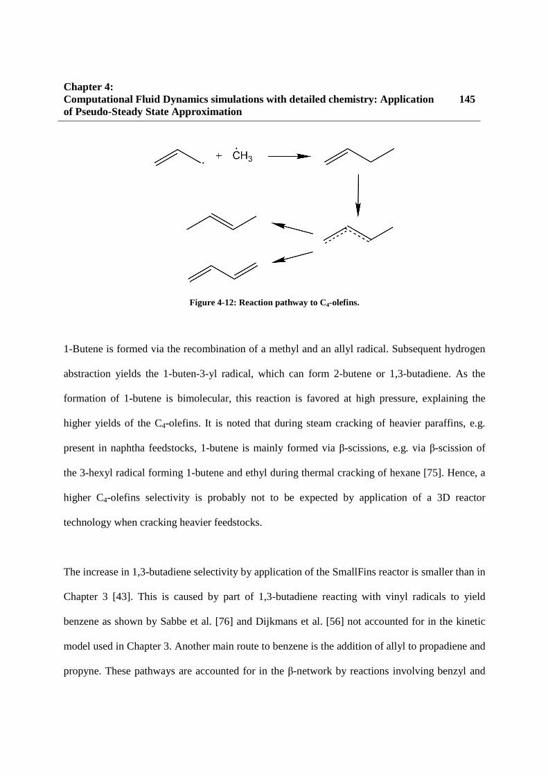
Chapter 4: Computational Fluid Dynamics simulations with detailed chemistry: Application of Pseudo-Steady State Approximation
145
Figure 4-12: Reaction pathway to C4-olefins.
1-Butene is formed via the recombination of a methyl and an allyl radical. Subsequent hydrogen
abstraction yields the 1-buten-3-yl radical, which can form 2-butene or 1,3-butadiene. As the
formation of 1-butene is bimolecular, this reaction is favored at high pressure, explaining the
higher yields of the C4-olefins. It is noted that during steam cracking of heavier paraffins, e.g.
present in naphtha feedstocks, 1-butene is mainly formed via β-scissions, e.g. via β-scission of
the 3-hexyl radical forming 1-butene and ethyl during thermal cracking of hexane [75]. Hence, a
higher C4-olefins selectivity is probably not to be expected by application of a 3D reactor
technology when cracking heavier feedstocks.
The increase in 1,3-butadiene selectivity by application of the SmallFins reactor is smaller than in
Chapter 3 [43]. This is caused by part of 1,3-butadiene reacting with vinyl radicals to yield
benzene as shown by Sabbe et al. [76] and Dijkmans et al. [56] not accounted for in the kinetic
model used in Chapter 3. Another main route to benzene is the addition of allyl to propadiene and
propyne. These pathways are accounted for in the β-network by reactions involving benzyl and

146 Chapter 4:
Computational Fluid Dynamics simulations with detailed chemistry: Application of Pseudo-Steady State Approximation
cyclopentadienyl radicals taken from the high temperature combustion kinetic model developed
by the CRECK modeling group [77]. As both these routes involve a bimolecular first reaction,
they are favored at higher pressure, i.e. in the SmallFins reactor. Based on these considerations
solely, a much higher increase in benzene selectivity would be expected in the SmallFins reactor.
However, both routes to benzene involve typical high-temperature species, i.e. vinyl and propyne
or propadiene respectively. Vinyl is formed by hydrogen abstraction from ethene, mainly by
methyl and hydrogen radicals which are hydrogen abstractions with high activation energies
(84.4 and 72.1 kJ/mol respectively). Propyne and propadiene are formed by a hydrogen
abstraction from propene to form propen-2-yl and a subsequent β-scission. Like the formation of
vinyl, the formation of propen-2-yl has a high activation energy. These considerations make that
the vinyl, propyne and propadiene yields are higher in the Bare reactor as shown in Figure 4-13.
Figure 4-13: Mixing cup average yield of vinyl radical [10-4 wt%] (A), propyne [10-4 wt%] (B) and propadiene
[10-4 wt%] (A) as a function of axial coordinate [m] in the 3D simulations of the industrial propane-cracking
reactor: - Bare; - SmallFins.

Chapter 4: Computational Fluid Dynamics simulations with detailed chemistry: Application of Pseudo-Steady State Approximation
147
Hence, the rate of formation of benzene in the SmallFins reactor in comparison to the Bare
reactor, is a balance between an increase caused by a higher pressure and a decrease caused by a
greater cross-sectional temperature uniformity. This statement is corroborated by Figure 4-14,
showing the benzene rate of formation as a function of radial coordinate at an axial coordinate of
7 m. In the reactor center, a higher rate of formation is seen in the SmallFins reactor caused by
the higher pressure. However, near the reactor inner wall, the rate of formation is lower caused by
the lower temperature. For the here adopted reactor designs, feedstock and process conditions,
the balance tips slightly in favor of the increase caused by the higher pressure. However, for other
designs, conditions and/or feedstocks, the opposite might hold, showing the need for these highly
detailed three-dimensional simulations upon evaluation of the application of a 3D reactor design
in a specific cracker.
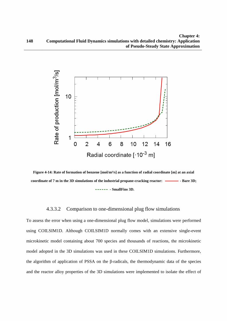
148 Chapter 4:
Computational Fluid Dynamics simulations with detailed chemistry: Application of Pseudo-Steady State Approximation
Figure 4-14: Rate of formation of benzene [mol/m³/s] as a function of radial coordinate [m] at an axial
coordinate of 7 m in the 3D simulations of the industrial propane-cracking reactor: - Bare 3D;
- SmallFins 3D.
4.3.3.2 Comparison to one-dimensional plug flow simulations
To assess the error when using a one-dimensional plug flow model, simulations were performed
using COILSIM1D. Although COILSIM1D normally comes with an extensive single-event
microkinetic model containing about 700 species and thousands of reactions, the microkinetic
model adopted in the 3D simulations was used in these COILSIM1D simulations. Furthermore,
the algorithm of application of PSSA on the β-radicals, the thermodynamic data of the species
and the reactor alloy properties of the 3D simulations were implemented to isolate the effect of

Chapter 4: Computational Fluid Dynamics simulations with detailed chemistry: Application of Pseudo-Steady State Approximation
149
the adopted reactor model on the simulation results. For the simulations of the Bare tube, 6� and
6? were set to unity, while for the SmallFins tube, 6� and 6? were set to 1.98 and 1.52
respectively, values obtained from the non-reactive flow simulations of Chapter 3.
Table 4-5 compares the 1D simulation results with the 3D simulation results of the two reactors
discussed above. For the two reactor designs, three 1D simulations were performed; without
radial profiles (1D), with a radial temperature profile (1D T) and with a radial temperature and β-
radicals profile (1D T, β). In all 1D simulations, the heat flux profile to the reactors was scaled to
obtain the same propane conversion as in the corresponding 3D simulation. In the 1D model
without radial profiles, the heat input necessary for the desired conversion is 1.5 % and 1.2 %
higher for the Bare and SmallFins reactor respectively. These errors are small but are significant
when considering that a similar error on the fuel flow rate to the furnace will be simulated when
performing coupled furnace-reactor simulations. When accounting for the radial temperature
profile, these differences decrease to 0.45 % and 0.66 % for the Bare and SmallFins reactor
respectively. Accounting for the radial non-uniformity of the β-radicals further reduces the
differences to 0.37 % and 0.49 %. The COT in the 1D simulations is higher than in the 3D
simulations. Taking into account radial profiles results in a closer agreement between the 1D and
3D simulated COT’s. The pressure drop in the Bare reactor is slightly overpredicted in the 1D
model compared to the 3D results. For the SmallFins reactor, a good agreement is obtained. This
shows that using a correction factor obtained from non-reactive CFD simulations can give
accurate pressure drop predictions for reactive 1D simulations. However, it should be noted that

150 Chapter 4:
Computational Fluid Dynamics simulations with detailed chemistry: Application of Pseudo-Steady State Approximation
the Reynolds number of the non-reactive simulation and this reactor simulation is the same which
is obviously important to obtain a correct scaling factor.
Figure 4-15A and B compare the external tube wall temperature (TMT) in the 3D and the 1D
simulations for the Bare and the SmallFins reactor respectively. For the Bare reactor, the
maximum tube metal temperature is overpredicted by 26 K using the 1D model without radial
profiles. As shown by Sundaram and Froment [41], the temperature difference between the inner
wall temperature and the mixing cup process gas temperature is indeed larger when using a
correlation for the Nusselt number derived for non-reactive flow than when accounting for the
endothermic reactions. Consequently, a good agreement is seen between 1D and 3D TMT’s
towards the end of the reactor where the endothermic heat of reaction is lower. Furthermore, axial
conduction in the tube metal is not accounted for in the 1D model, which flattens out the TMT
profile in the 3D simulations, reducing the TMT maximum. Taking into account the effect of
only the radial temperature and also β-radicals concentration profile reduces the overprediction of
the maximum TMT to 20 and 13 K respectively. Similar considerations as made for the Bare
reactor can be made for the SmallFins reactor, with a maximum TMT difference compared to the
3D simulation equal to 20, 18 and 14 K for 1D, 1D T and 1D T, β respectively.

Chapter 4: Computational Fluid Dynamics simulations with detailed chemistry: Application of Pseudo-Steady State Approximation
151
Figure 4-15: External tube metal temperature [K] for the Bare (A) and SmallFins (B) reactor: - Bare
3D; - Bare 1D; - Bare 1D T; - Bare 1D T, β.
Figure 4-16 shows the propane conversion for the three-dimensional and the one-dimensional
simulations of the Bare reactor. Without accounting for radial profiles, the induction length for
reaction to start is longer compared to the 3D simulation. When accounting for radial temperature
and β-radical concentrations in the 1D simulations, the agreement with the 3D conversion profile
at the start of the reactor is better as seen from the insert in Figure 4-16.
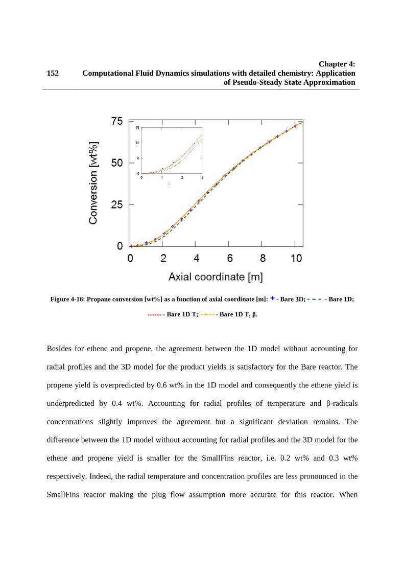
152 Chapter 4:
Computational Fluid Dynamics simulations with detailed chemistry: Application of Pseudo-Steady State Approximation
Figure 4-16: Propane conversion [wt%] as a function of axial coordinate [m]: - Bare 3D; - Bare 1D;
- Bare 1D T; - Bare 1D T, β.
Besides for ethene and propene, the agreement between the 1D model without accounting for
radial profiles and the 3D model for the product yields is satisfactory for the Bare reactor. The
propene yield is overpredicted by 0.6 wt% in the 1D model and consequently the ethene yield is
underpredicted by 0.4 wt%. Accounting for radial profiles of temperature and β-radicals
concentrations slightly improves the agreement but a significant deviation remains. The
difference between the 1D model without accounting for radial profiles and the 3D model for the
ethene and propene yield is smaller for the SmallFins reactor, i.e. 0.2 wt% and 0.3 wt%
respectively. Indeed, the radial temperature and concentration profiles are less pronounced in the
SmallFins reactor making the plug flow assumption more accurate for this reactor. When

Chapter 4: Computational Fluid Dynamics simulations with detailed chemistry: Application of Pseudo-Steady State Approximation
153
analyzing the effect of the reactor geometry on the product selectivities, it is seen that only for
some products the right trends are predicted by the 1D model, even when radial profiles of
temperature and β-radicals are accounted for. The increase in methane, propene and benzene
selectivity by application of the SmallFins reactor is well captured. On the contrary, the decrease
in ethene selectivity and the small increase in C4-(di)olefins selectivity is not captured by the 1D
T,β model.
4.4 Conclusions A methodology was developed to adopt detailed kinetic models in computational fluid dynamics
simulations of steam cracking reactors. Eventually 3D simulations should become the industrial
standard for design because comparison to 1D plug flow reactor simulations shows that a small
but significant error is made by neglecting the increased reaction rates in the film near the reactor
inner wall. Significant speedup in the 3D simulations was achieved by a combination of three
techniques. Firstly, the application of the µ-radical hypothesis and PSSA on µ-radicals during
network generation reduces the number of and the stiffness of the species continuity equations.
Secondly, on the fly application of the PSSA on the β(µ)-radicals further reduces the number of
continuity equations and the stiffness of the system. Finally, Maple®’s CodeGeneration package
was used to generate an optimal calculation procedure for the reaction rates and the rates of
formation. Depending on the kinetic model’s size, a speedup factor from 7.4 to 54.2 was obtained
compared to the standard FLUENT routines. A good agreement was seen for the species yields
compared to the conventional 3D simulations. The deviations are the largest for the radicals
weight fraction near the reactor inner wall with an average relative error of 10 %, which could be
154 Chapter 4:
Computational Fluid Dynamics simulations with detailed chemistry: Application of Pseudo-Steady State Approximation
significant for example when fundamental coking models are considered. Application to a
propane-cracking conventional bare reactor and a helicoidally finned reactor shows that
considering a kinetic model of 85 species, the finned reactor outperforms the bare reactor if only
coke formation is considered as the maximum tube temperature was reduced by 44 K. However,
the ethene selectivity is reduced by 0.17 % while propene and 1,3-butadiene selectivity increased
by 0.08 and 0.03 % respectively. Reaction path analysis on the detailed kinetic model reveals that
the change in ethene and propene selectivity are correlated as less propene is converted to ethene
in the SmallFins reactor because of the lower hydrogen radical concentration. The increase in
1,3-butadiene is caused by the higher pressure drop as the first step in 1,3-butadiene formation is
the bimolecular recombination of methyl and allyl. Also the benzene selectivity is 0.05 wt%
higher in the SmallFins reactor because of the higher pressure drop. Accounting for radial
temperature and radicals concentration profiles in a 1D model, improves the agreement between
the 1D and 3D simulated heat input, tube metal temperature and coil-outlet temperature.
However, the effect of a 3D reactor technology on product selectivities is not well captured by a
1D model. Accounting for radial temperature and radicals concentration profiles only results in a
marginal improvement. This illustrates the need for 3D reactor simulations upon economic
evaluation of a 3D reactor technology, where the trade-off between the run length improvement
and the change in products selectivity is key.

Chapter 4: Computational Fluid Dynamics simulations with detailed chemistry: Application of Pseudo-Steady State Approximation
155
References [1] R. Vinu, L.J. Broadbelt, Unraveling Reaction Pathways and Specifying Reaction Kinetics for Complex Systems, in: J.M. Prausnitz (Ed.) Annual Review of Chemical and Biomolecular Engineering, Vol 3, 2012, pp. 29-54. [2] E. Ranzi, T. Faravelli, P. Gaffuri, A. Sogaro, Low-temperature combustion: Automatic generation of primary oxidation reactions and lumping procedures, Combustion and Flame, 102 (1995) 179-192. [3] G.M. Côme, V. Warth, P.A. Glaude, R. Fournet, F. Battin-Leclerc, G. Scacchi, Computer-aided design of gas-phase oxidation mechanisms—Application to the modeling of n-heptane and iso-octane oxidation, Symposium (International) on Combustion, 26 (1996) 755-762. [4] L.J. Broadbelt, S.M. Stark, M.T. Klein, Computer-generated pyrolysis modeling - On the fly generation of species, reactions and rates, Industrial & Engineering Chemistry Research, 33 (1994) 790-799. [5] W.H. Green, J.W. Allen, R.W. Ashcraft, G.J. Beran, C.F. Goldsmith, M.R. Harper, A. Jalan, G.R. Magoon, D.M. Matheu, S. Petway, S. Raman, S. Sharma, K.M. Van Geem, J. Song, J. Wen, R.H. West, A. Wong, H.-W. Wong, P.E. Yelvington, Y. J., RMG - Reaction Mechanism Generator v3.3, 2011. [6] N.M. Vandewiele, K.M. Van Geem, M.F. Reyniers, G.B. Marin, Genesys: Kinetic model construction using chemo-informatics, Chemical Engineering Journal, 207 (2012) 526-538. [7] E.S. Blurock, Detailed mechanism generation. 1. Generalized reactive properties as reaction class substructures, Journal of Chemical Information and Computer Sciences, 44 (2004) 1336-1347. [8] E.S. Blurock, Detailed mechanism generation. 2. Aldehydes, ketones, and olefins, Journal of Chemical Information and Computer Sciences, 44 (2004) 1348-1357. [9] S. Rangarajan, A. Bhan, P. Daoutidis, Language-oriented rule-based reaction network generation and analysis: Description of RING, Computers & Chemical Engineering, 45 (2012) 114-123. [10] S. Rangarajan, A. Bhan, P. Daoutidis, Language-oriented rule-based reaction network generation and analysis: Applications of RING, Computers & Chemical Engineering, 46 (2012) 141-152. [11] O. Herbinet, W.J. Pitz, C.K. Westbrook, Detailed chemical kinetic oxidation mechanism for a biodiesel surrogate, Combustion and Flame, 154 (2008) 507-528. [12] P.A. Glaude, O. Herbinet, S. Bax, J. Biet, V. Warth, F. Battin-Leclerc, Modeling of the oxidation of methyl esters-Validation for methyl hexanoate, methyl heptanoate, and methyl decanoate in a jet-stirred reactor, Combustion and Flame, 157 (2010) 2035-2050. [13] K.M. Van Geem, M.F. Reyniers, G.B. Marin, Challenges of modeling steam cracking of heavy feedstocks, Oil & Gas Science and Technology-Revue De L Institut Francais Du Petrole, 63 (2008) 79-94. [14] M.W.M. van Goethem, F.I. Kleinendorst, C. van Leeuwen, N. van Velzen, Equation-based SPYRO® model and solver for the simulation of the steam cracking process, Computers & Chemical Engineering, 25 (2001) 905-911.

156 Chapter 4:
Computational Fluid Dynamics simulations with detailed chemistry: Application of Pseudo-Steady State Approximation
[15] T. Lu, C.K. Law, Toward accommodating realistic fuel chemistry in large-scale computations, Progress in Energy and Combustion Science, 35 (2009) 192-215. [16] T. Dijkmans, C.M. Schietekat, K.M. Van Geem, G.B. Marin, GPU based simulation of reactive mixtures with detailed chemistry in combination with tabulation and an analytical Jacobian, Computers & Chemical Engineering, 71 (2014) 521-531. [17] L. Tosatto, B.A.V. Bennett, M.D. Smooke, A transport-flux-based directed relation graph method for the spatially inhomogeneous instantaneous reduction of chemical kinetic mechanisms, Combustion and Flame, 158 (2011) 820-835. [18] M. Boileau, G. Staffelbach, B. Cuenot, T. Poinsot, C. Berat, LES of an ignition sequence in a gas turbine engine, Combustion and Flame, 154 (2008) 2-22. [19] G. Hu, H. Wang, F. Qian, Y. Zhang, J. Li, K.M. Van Geem, G.B. Marin, Comprehensive CFD Simulation of Product Yields and Coking Rates for a Floor- and Wall-Fired Naphtha Cracking Furnace, Industrial & Engineering Chemistry Research, 50 (2011) 13672-13685. [20] L. Liang, J.G. Stevens, J.T. Farrell, A Dynamic Multi-Zone Partitioning Scheme for Solving Detailed Chemical Kinetics in Reactive Flow Computations, Combustion Science and Technology, 181 (2009) 1345-1371. [21] M. Bodenstein, Eine Theorie der photochemischen Reaktionsgeschwindigkeiten, Zeitschrift für Physikalische Chemie, 85 (1913) 329-397. [22] D.A. Frank-Kamenetskii, Conditions for the applicability of the Bodenstein method in chemical kinetics, Zhurnal Fizicheskoy Himii, 14 (1940). [23] T. Turanyi, A.S. Tomlin, M.J. Pilling, On the error of the quasi-steady-state approximation, Journal of Physical Chemistry, 97 (1993) 163-172. [24] T. Kovács, I.G. Zsély, Á. Kramarics, T. Turányi, Kinetic analysis of mechanisms of complex pyrolytic reactions, Journal of Analytical and Applied Pyrolysis, 79 (2007) 252-258. [25] D.L. Chapman, L.K. Underhill, The interaction of chlorine and hydrogen. The influence of mass., Journal of the Chemical Society, Transactions, 103 (1913) 496-508. [26] J.Y. Chen, A general procedure for constructing reduced reaction-mechanisms with given independent relations, Combustion Science and Technology, 57 (1988) 89-94. [27] N. Peters, F.A. Williams, The asymptotic structure of stoichiometric methane air flames, Combustion and Flame, 68 (1987) 185-207. [28] E. Ranzi, M. Dente, A. Goldaniga, G. Bozzano, T. Faravelli, Lumping procedures in detailed kinetic modeling of gasification, pyrolysis, partial oxidation and combustion of hydrocarbon mixtures, Progress in Energy and Combustion Science, 27 (2001) 99-139. [29] M. Dente, G. Bozzano, T. Faravelli, A. Marongiu, S. Pierucci, E. Ranzi, Kinetic Modelling of Pyrolysis Processes in Gas and Condensed Phase, in: G.B. Marin (Ed.) Advances in Chemical Engineering, Academic Press, 2007, pp. 51-166. [30] U. Maas, S.B. Pope, Simplifying chemical-kinetics: Intrinsic low-dimensional manifolds in composition space, Combustion and Flame, 88 (1992) 239-264. [31] T. Lu, C.K. Law, On the applicability of directed relation graphs to the reduction of reaction mechanisms, Combustion and Flame, 146 (2006) 472-483. [32] T.F. Lu, Y.G. Ju, C.K. Law, Complex CSP for chemistry reduction and analysis, Combustion and Flame, 126 (2001) 1445-1455.

Chapter 4: Computational Fluid Dynamics simulations with detailed chemistry: Application of Pseudo-Steady State Approximation
157
[33] S.B. Pope, Computationally efficient implementation of combustion chemistry using in situ adaptive tabulation, Combustion Theory and Modelling, 1 (1997) 41-63. [34] S.R. Tonse, N.W. Moriarty, N.J. Brown, M. Frenklach, PRISM: Piecewise reusable implementation of solution mapping. an economical strategy for chemical kinetics, Isr. J. Chem., 39 (1999) 97-106. [35] D.A. Schwer, P.S. Lu, W.H. Green, An adaptive chemistry approach to modeling complex kinetics in reacting flows, Combustion and Flame, 133 (2003) 451-465. [36] I. Banerjee, M.G. Ierapetritou, An adaptive reduction scheme to model reactive flow, Combustion and Flame, 144 (2006) 619-633. [37] M. Valorani, F. Creta, D.A. Goussis, J.C. Lee, H.N. Najm, An automatic procedure for the simplification of chemical kinetic mechanisms based on CSP, Combustion and Flame, 146 (2006) 29-51. [38] L. Liang, J.G. Stevens, S. Raman, J.T. Farrell, The use of dynamic adaptive chemistry in combustion simulation of gasoline surrogate fuels, Combustion and Flame, 156 (2009) 1493-1502. [39] K.Y. He, M.G. Ierapetritou, I.P. Androulakis, Integration of On-The-Fly Kinetic Reduction with Multidimensional CFD, AIChE Journal, 56 (2010) 1305-1314. [40] V. Gnielinski, New equations for heat and mass-transfer in turbulent pipe and channel flow, International Chemical Engineering, 16 (1976) 359-368. [41] K.M. Sundaram, G.F. Froment, A comparison of simulation models for empty tubular reactors, Chemical Engineering Science, 34 (1979) 117-124. [42] K.M. Van Geem, G.J. Heynderickx, G.B. Marin, Effect of radial temperature profiles on yields in steam cracking, AIChE Journal, 50 (2004) 173-183. [43] C.M. Schietekat, D.J. Van Cauwenberge, K.M. Van Geem, G.B. Marin, Computational fluid dynamics-based design of finned steam cracking reactors, AIChE Journal, 60 (2014) 794-808. [44] G.J. Heynderickx, G.G. Cornelis, G.F. Froment, Circumferential tube skin temperature profiles in thermal cracking coils, AIChE Journal, 38 (1992) 1905-1912. [45] C.M. Schietekat, M.W.M. van Goethem, K.M. Van Geem, G.B. Marin, Swirl flow tube reactor technology: An experimental and computational fluid dynamics study, Chemical Engineering Journal, 238 (2014) 56-65. [46] M.W.M. van Goethem, E. Jelsma, Numerical and experimental study of enhanced heat transfer and pressure drop for high temperature applications, Chemical Engineering Research & Design, 92 (2014) 663-671. [47] K.M. Sundaram, G.F. Froment, Two dimensional model for the simulation of tubular reactors for thermal cracking, Chemical Engineering Science, 35 (1980) 364-371. [48] J.C. Fagley, Simulation of transport in laminar, tubular reactors and application to ethane pyrolysis, Industrial & Engineering Chemistry Research, 31 (1992) 58-69. [49] L.J. Velenyi, Y. Song, J.C. Fagley, Carbon deposition in ethane pyrolysis reactors, Industrial & Engineering Chemistry Research, 30 (1991) 1708-1712. [50] J.J. De Saegher, T. Detemmerman, G.F. Froment, Three dimensional simulation of high severity internally finned cracking coils for olefins production, Revue De L'Institut Français Du Pétrole, 51 (1996) 245-260.

158 Chapter 4:
Computational Fluid Dynamics simulations with detailed chemistry: Application of Pseudo-Steady State Approximation
[51] T. Detemmerman, G.F. Froment, Three dimensional coupled simulation of furnaces and reactor tubes for the thermal cracking of hydrocarbons, Revue De L'Institut Français Du Pétrole, 53 (1998) 181-194. [52] X. Lan, J. Gao, C. Xu, H. Zhang, Numerical simulation of transfer and reaction processes in ethylene furnaces, Chemical Engineering Research & Design, 85 (2007) 1565-1579. [53] J.V. Albano, K.M. Sundaram, M.J. Maddock, Applications of Extended Surfaces in Pyrolysis Coils, Energy Progress, 8 (1988) 160-168. [54] C.F. Colebrook, Turbulent flow in pipes, with particular reference to the transition region between smooth and rough pipe laws, Journal of the Institution of Civil Engineers, 11 (1939). [55] L. Prandtl, The mechanics of viscous fluids, Aerodynamics Theory, 3 (1935). [56] T. Dijkmans, S.P. Pyl, M.-F. Reyniers, R. Abhari, K.M. Van Geem, G.B. Marin, Production of bio-ethene and propene: alternatives for bulk chemicals and polymers, Green Chemistry, 15 (2013) 3064-3076. [57] P.J. Clymans, G.F. Froment, Computer-generation of reaction paths and rate-equations in the thermal-cracking of normal and branched paraffins, Computers & Chemical Engineering, 8 (1984) 137-142. [58] L.P. Hillewaert, J.L. Dierickx, G.F. Froment, Computer-Generation of Reaction Schemes and Rate-Equations for Thermal Cracking, AIChE Journal, 34 (1988) 17-24. [59] M.K. Sabbe, F. De Vleeschouwer, M.F. Reyniers, M. Waroquier, G.B. Marin, First Principles Based Group Additive Values for the Gas Phase Standard Entropy and Heat Capacity of Hydrocarbons and Hydrocarbon Radicals, J. Phys. Chem. A, 112 (2008) 12235-12251. [60] M.K. Sabbe, M. Saeys, M.F. Reyniers, G.B. Marin, V. Van Speybroeck, M. Waroquier, Group additive values for the gas phase standard enthalpy of formation of hydrocarbons and hydrocarbon radicals, J. Phys. Chem. A, 109 (2005) 7466-7480. [61] M.K. Sabbe, M.F. Reyniers, V. Van Speybroeck, M. Waroquier, G.B. Marin, Carbon-centered radical addition and beta-scission reactions: Modeling of activation energies and pre-exponential factors, ChemPhysChem, 9 (2008) 124-140. [62] M.K. Sabbe, M.F. Reyniers, M. Waroquier, G.B. Marin, Hydrogen Radical Additions to Unsaturated Hydrocarbons and the Reverse beta-Scission Reactions: Modeling of Activation Energies and Pre-Exponential Factors, ChemPhysChem, 11 (2010) 195-210. [63] M.K. Sabbe, A.G. Vandeputte, M.F. Reyniers, M. Waroquier, G.B. Marin, Modeling the influence of resonance stabilization on the kinetics of hydrogen abstractions, PCCP, 12 (2010) 1278-1298. [64] Lu, C.K. Law, Systematic Approach To Obtain Analytic Solutions of Quasi Steady State Species in Reduced Mechanisms, The Journal of Physical Chemistry A, 110 (2006) 13202-13208. [65] Z.Y. Ren, S.B. Pope, Entropy production and element conservation in the quasi-steady-state approximation, Combustion and Flame, 137 (2004) 251-254. [66] R.J. Kee, F.M. Rupley, J.A. Miller, M.E. Coltrin, J.F. Grcar, E. Meeks, H.K. Moffat, G. Lutz, A.E. Dixon-Lewis, M.D. Smooke, J. Warnatz, G.H. Evans, R.S. Larson, R.E. Mitchell, L.R. Petzhold, W.C. Reynolds, M. Caracotsios, W.E. Stewart, P. Glarborg, C. Wang, O. Adigun, W.G. Houf, C.P. Chou, S.F. Miller, P. Ho, D.J. Young, CHEMKIN Release 4.1.1, Reaction Design, Inc., San Diego, CA, USA, 2007.

Chapter 4: Computational Fluid Dynamics simulations with detailed chemistry: Application of Pseudo-Steady State Approximation
159
[67] S. Li, L. Petzold, Design of New DASPK for Sensitivity Analysis, UCSB Technical report., (1999). [68] L. Shengtai, P. Linda, Design of new Daspk for Sensitivity Analysis, University of California at Santa Barbara, 1999. [69] T. Kovacs, I.G. Zsely, A. Kramarics, T. Turanyi, Kinetic analysis of mechanisms of complex pyrolytic reactions, Journal of Analytical and Applied Pyrolysis, 79 (2007) 252-258. [70] P.M. Plehiers, G.C. Reyniers, G.F. Froment, Simulation of the run length of an ethane cracking furnace, Industrial & Engineering Chemistry Research, 29 (1990) 636-641. [71] G.J. Heynderickx, G.F. Froment, Simulation and comparison of the run length of an ethane cracking furnace with reactor tubes of circular and elliptical cross sections, Industrial & Engineering Chemistry Research, 37 (1998) 914-922. [72] S. Wauters, G.B. Marin, Kinetic Modeling of Coke Formation during Steam Cracking, Industrial & Engineering Chemistry Research, 41 (2002) 2379-2391. [73] S. Wauters, G.B. Marin, Computer generation of a network of elementary steps for coke formation during the thermal cracking of hydrocarbons, Chemical Engineering Journal, 82 (2001) 267-279. [74] Y.-R. Luo, Handbook of bond dissociation energies in organic compounds, CRC Press, Boca Raton, Florida, 2003. [75] K.M. Van Geem, M.F. Reyniers, G.B. Marin, J. Song, W.H. Green, D.M. Matheu, Automatic reaction network generation using RMG for steam cracking of n-hexane, AIChE Journal, 52 (2006) 718-730. [76] M.K. Sabbe, K.M. Van Geem, M.-F. Reyniers, G.B. Marin, First principle-based simulation of ethane steam cracking, AIChE Journal, 57 (2011) 482-496. [77] C. Cavallotti, D. Polino, A. Frassoldati, E. Ranzi, Analysis of Some Reaction Pathways Active during Cyclopentadiene Pyrolysis, The Journal of Physical Chemistry A, 116 (2012) 3313-3324.

160 Chapter 4:
Computational Fluid Dynamics simulations with detailed chemistry: Application of Pseudo-Steady State Approximation

Chapter 5: The importance of turbulence-chemistry interaction for CFD simulations
161
Chapter 5:
The importance of turbulence-chemistry
interaction for CFD simulations

162 Chapter 5: The importance of turbulence-chemistry interaction for CFD simulations
5.1 Introduction Modeling finite-rate chemistry in turbulent reactive flows presents a challenge because of the
large span in length and time scales. In Large Eddy Simulations (LES) or Direct Numerical
Simulations (DNS), the largest or all turbulent time scales are explicitly resolved, implying that
local fluctuations and their effect on reaction rates are explicitly accounted for. Although
requiring stringent computational resources, LES turbulence models have been successfully
applied to reactive flows and this mainly in combustion research [1-6]. The present work focuses
on steam cracking of hydrocarbons, i.e. pyrolysis, and although pyrolysis reactions are inherently
a part of kinetic models for combustion, the simulation requirements for combustion and steam
cracking are quite different. Indeed, as often the main objectives of a CFD simulation of a
combustion process are the prediction of heat release, flame temperature and flame stability,
reduced kinetic models and/or mixture fraction approaches are typically sufficient. The main
exception is the simulation of ��� formation during combustion which requires a detailed kinetic
model. However, ��� formation is mostly calculated in a post-processing step, decoupling the
flow dynamics from the ��� chemistry calculation [7]. On the contrary, one of the paramount
objectives of any simulation of a steam cracking reactor, whether with a plug flow reactor model
or using a CFD model, is the accurate simulation of product yields. Whereas typically
combustion proceeds to full conversion to steam and carbon dioxide, steam cracking reactors are
operated at a partial conversion to maximize the production of valuable light olefins. These two
observations mean that the minimum size of the kinetic models necessary for steam cracking
reactor simulations is larger than that required for typical combustion simulations. Secondly, the
Reynolds number in industrial steam cracking reactors ranges from 80,000 to more than 200,000

Chapter 5: The importance of turbulence-chemistry interaction for CFD simulations
163
[8]. The grid requirements for wall-resolved LES scale to the power of 1.8 with the Reynolds
number [9, 10], currently limiting LES to Reynolds numbers of approximately 100,000. The
combination of the large kinetic model and the large grid size renders a spatial LES of an
industrial steam cracking reactor computationally very demanding. Therefore Reynolds Averaged
turbulence models are used in this work. However, neglect of the turbulent fluctuations by using
the mean temperature and concentrations for the calculation of reaction rates can induce an error:
�� ≠ ���,� �� (5.1)
and this mainly due to the highly nonlinear dependence of the reaction rate coefficient on
temperature in the Arrhenius equation:
��� ≠ ���� = ������,���� (5.2)
The effect of turbulent fluctuations on the reaction rates can be accounted for in RANS
simulations by scalar-variance transport equations for temperature and species concentrations. As
the temperature dependence (exponential) is stronger than the concentration dependence (first or
second order in pyrolysis kinetic models), only the effect of temperature fluctuations is accounted
for here. Scalar-variance transport equations have been used for several applications. One of the
most important being the simulation of turbulent premixed flames [11-13]. In order to reduce the
computational load in this application, a chemistry model based on elementary reactions is
eliminated. Instead, a so-called reaction progress variable is introduced which is defined in such a
way that it spans the interval between unburned and fully burned fuel by increasing
monotonically from zero to one. Transport equations for the progress variable mean and variance
are solved and the species concentrations are reconstructed in a post-processing step based on a
predefined probability density function (PDF) of the reaction progress variable. Scalar-variance

164 Chapter 5: The importance of turbulence-chemistry interaction for CFD simulations
transport equations have also been used to predict ��� formation in turbulent combustion [7]. In
a post-processing step, the formation rate of ��� is calculated based on the temperature mean
and variance and mean species concentrations.
In this work, a code for the three-dimensional simulation of steam cracking reactors based on the
free and open source CFD package OpenFOAM® was developed [14, 15]. The effect of turbulent
temperature fluctuations on the reaction rates can be accounted for by solving a temperature
variance transport equation. It should be noted that in contrast to non-premixed combustion, the
reactants in steam cracking reactors are (pre)mixed. Hence, the effect of finite-rate mixing by e.g.
the Eddy Dissipation Concept [16] or the Eddy Breakup Model [17] is not accounted for here.
Pseudo-steady state is applied to the radicals as discussed in Chapter 4 to limit the computational
cost while maintaining the chemical detail. To further reduce the computational cost, the code
also incorporates a dynamic zoning method. In the rest of the chapter, the model equations are
summarized and the solution procedures are discussed. Next, the importance of turbulence-
chemistry interaction in steam cracking reactors is assessed and an industrial reactor is simulated.
5.2 Model equations
Conservation equations 5.2.1
Steam cracking reactors are gas-phase flow tubular reactors made out of high Cr-Ni-alloy steels.
To account for the conductive heat transfer in the reactor metal, next to the process gas region,
also the solid metal region is modeled. The process is non-isothermal and non-isobaric and hence
the solution of both the momentum and the energy equation is required for the process gas. The
process gas can be considered as an ideal gas mixture. In the reactor metal region, only the

Chapter 5: The importance of turbulence-chemistry interaction for CFD simulations
165
conductive heat transfer equation is solved. The governing steady-state conservation equations
are summarized in Table 5-1. Turbulence can be taken into account using any of the available
standard RANS turbulence models of OpenFOAM® or new user-implemented turbulence models.
Table 5-1: Conservation equations.
Process gas region
Global mass ∇ ∙ ���� = 0 (5.3)
Momentum ∇ ∙ ������ = −∇� + ∇ ∙ !" (5.4)
Energy ∇ ∙ #��� $ℎ + 12 |��|)*+ = ∇ ∙ #,-,.--�/0 ∇ℎ+ + 23 (5.5)
Species ∇ ∙ 4��567 = −∇ ∙ 48.--,6∇567 + 96 , ∀; = 1, <=��/ − 1 (5.6)
Reactor metal region
Energy ∇ ∙ �,>∇ = 0 (5.7)
In the Navier-Stokes equations, the laminar viscosity of the ideal gas mixture is calculated from
the species laminar viscosity using an ideal mixing law. The species laminar viscosities ?@,6 are
calculated from kinetic theory using the species Lennard-Jones well depth ABC and DBC, i.e. the
distance at which the intermolecular potential between the two particles is zero; ?@,6 = E FFG�HIJ,GK LM�G∗O
with Ω�∗ = 1.16145∗�U.VWXYW + 0.52487��U.YY\)�∗ + 2.16178��).W\YXY�∗ and ∗ = ]^�_IJ,G .
Most values for ABC and DBC are taken from literature [18], with the remaining estimated using
RMG’s TransportDataEstimator [19]. In the energy equation (5.5), a,baacde is the thermal diffusivity

166 Chapter 5: The importance of turbulence-chemistry interaction for CFD simulations
containing contributions of laminar and turbulent diffusion, i.e. ,-,.-- = ,-,@ + ,-,f. The laminar
conductivity coefficient ,-,@ is calculated from kinetic theory, i.e. ,-,@,6 = ?@,6 M/0,6 + gW9O. The
turbulent conductivity coefficient ,-,f is calculated from the turbulent viscosity, i.e. ,-,f = hijki with l�f = 0.85 . The heat of reaction 23 is calculated from the species heat of formation:
23 = ∑ 96Δ-,6ℎo>0.d6pV . The species continuity equations (5.6) are solved for <=��/ − 1 species
with the concentration of the last species calculated from the global mass balance (5.3). Steam is
chosen as the last component because it is present in the entire reactor in a considerable
concentration because in the process it is added as a diluent. Furthermore, steam is considered to
be inert in the here adopted reaction mechanisms and hence the uniformity of the steam mass
fraction over the reactor acts as a double check for convergence and mass conservation of the
simulation. The effective diffusion coefficient 8.--,6 in the species continuity equations has a
laminar and a turbulent contribution; 8.--,6 = 8@,6 + 8f,6. The laminar coefficient is neglected as
its contribution is minor in comparison to the turbulent contribution which is calculated from the
turbulent viscosity, i.e. 8f,6 = hiqdi with 2/f = 0.7 [20].
To account for the effect of local turbulent fluctuations on the reaction rates a temperature
probability density function is used as explained in 5.3.2. The temperature variance is obtained by
solving the scalar variance equation (5.8). The derivation of this equation is shown in Fox [21]
and relies on the eddy diffusivity concept of Kolmogorov’s theory for the unclosed terms. The
laminar transport contribution in the first term in the right-hand side of equation (5.8) is neglected
because of the high Reynolds numbers.

Chapter 5: The importance of turbulence-chemistry interaction for CFD simulations
167
∇ ∙ ����D�) = ∇ ∙ M� ?f0.85∇D�)O + 2 ?f2/f �∇� ) − A� (5.8)
There are two distinct ways of obtaining the temperature variance dissipation A� . In fully
developed flow at high Reynolds numbers, the algebraic ‘equilibrium’ model, i.e. equation (5.8),
can be used [21]. The parameter 5V is typically set to 2.0 based on the experimental work of
Beguier et al [22].
A� = 5V A� D�) (5.9)
For non-fully developed flow, the effect of turbulence anisotropy and mean shear stress can be
accounted for by modeling an extra transport equation for the temperature variance dissipation
(5.10).
∇����A� = ∇ ∙ $� ?f2/f ∇A�* − 5)� A�D�) − 5\�) 5h�?f A� + 5W �5h�2/f �∇� ) + 5g?f �� rstr (5.10)
The terms with the model parameters 5) and 5\ are the respective dissipation terms due to scalar
and mechanical destruction of fluctuations. The terms with the model parameters 5W and 5g are
the respective production terms due to scalar gradients and velocity gradients. Many sets of
values have been proposed for the model parameters 5), 5\, 5W and 5g. An extensive overview is
given by Sanders and Gokalp [23]. The model parameter 5h is part of the turbulence model and
equal to 0.09 in most k-ε turbulence models. The source term rstr is the strain rate tensor defined
as:
2�6 = 12#uv��uw6 + uv�6uw� + (5.11)
Based on user-input, turbulence-chemistry interaction can or cannot be taken into account. If
turbulence-chemistry is accounted for, the ‘equilibrium’ closure model, i.e. equation (5.9), or one

168 Chapter 5: The importance of turbulence-chemistry interaction for CFD simulations
of the fifteen sets of implemented parameter values for equation (5.10) can be used. To assure
convergence, iterations are performed until the final residuals of all equations are below 10�Vg and below 10�VX for the gas region energy equation. Furthermore, the outlet mixing cup
temperature and species concentrations are monitored to be constant during the final 100
iterations.
Species rate of formation 5.2.2
As discussed in Chapter 1 thermal cracking of hydrocarbons proceeds mainly through a radical
mechanism [24-26]. The adopted kinetic models in this work are single-event microkinetic
models that only take into account elementary reactions. The kinetic models were derived from
the model of Van de Vijver et al. [27] by removing species known to be unimportant during
cracking of the considered feedstock molecule. The validity of the reduced network is shown in
Appendix A by comparing one-dimensional plug flow simulation results obtained with the
reduced and the full model to pilot plant data. Thermodynamic data of most molecules and
radicals was derived from first principles CBS-QB3 calculations of Sabbe et al. [28, 29]. Missing
data was estimated using RMG’s ThermoDataEstimator [19]. To avoid time-consuming
calculation of reverse reaction rates, reversible reactions are decoupled into two irreversible
reactions with the Arrhenius parameters of the reverse reaction calculated prior to the simulation
via regression to the values expressed by thermodynamic consistency over the relevant
temperature range from 700 to 1300 K.
A probability density function (PDF) is used to calculate the average reaction rate coefficients to
account for turbulence-chemistry interaction:

Chapter 5: The importance of turbulence-chemistry interaction for CFD simulations
169
��� = x ��� l� yzU (5.12)
with ��� the mean reaction rate coefficient used for the calculation of the reaction rate �� =���∏ |�,656}�,Go>0.d6pV . A predefined Gaussian probability function distribution for temperature is
assumed:
l� = 1�2~D�) V) �
������ K)H�K (5.13)
With � the mean temperature obtained by solving the energy equation (5.5) and D�) the
temperature variance. The temperature variance transport equation (5.8) is solved to obtain a
value for D�) in each grid cell.
5.3 Solution procedure
Conservation equations 5.3.1
OpenFOAM® applies the finite-volume method on collocated grids and adopts Gaussian
integration. A segregated solver was used to solve the conservation equations given in Table 5-1.
The Semi-Implicit Method for Pressure-Linked Equations (SIMPLE) algorithm was used to solve
the Navier-Stokes equations. The mesh orthogonality was high enough in all simulations, not to
require any non-orthogonal correctors. A 2nd order central differencing spatial discretization
scheme was used, with a limiter for the species mass fractions to be non-negative and below or
equal to unity. As turbulence model, the shear-stress transport (SST) k-ω model was used to
calculate the eddy viscosity [30]. Using detailed kinetic models renders the species conservation
equations highly stiff because of the large difference in time scales associated with species and
reactions as discussed in Chapter 1. To tackle this issue, the pseudo-steady state assumption

170 Chapter 5: The importance of turbulence-chemistry interaction for CFD simulations
(PSSA) is applied on the radicals on-the fly using a numerical algebraic solver. Besides reducing
the stiffness of the species conservation equations, also the number of species conservation
equations is reduced as the concentrations of the PSS species is calculated in the algebraic solver
based on the concentrations of the non-PSS species. A more elaborate discussion on the adopted
algorithm using FLUENT® was given in Chapter 4.
Turbulence-chemistry interaction 5.3.2
When turbulence-chemistry interaction is accounted for, the integral in equation (5.12) has to be
integrated in each cell at every iteration. Combination of equation (5.12) and (5.13) gives the
following expression for the mean reaction rate coefficient:
��� = ���� = �2~D�) �V/)x �� exp $−��,�9* exp #−� − � )
2D�) +yz�z (5.14)
A linear transformation of to the normalized variable w is performed. The resulting expression
for the mean reaction rate coefficient is given below.
w = − ��2D�) V/) (5.15)
��� = ~�V/)x �� exp #− ��,�9��2D�) V/)w + � + exp�−w) ywz�z (5.16)

Chapter 5: The importance of turbulence-chemistry interaction for CFD simulations
171
The right-hand side of this expression can be rewritten as:
~�V/)x exp�−w) ��� exp #− ��,�9��2D�) V/)w + � +� ywz�z
= ~�V/)x ��w ��w ywz�z
(5.17)
with ��w = exp�−w) and ��w = �� exp #− ��,��M4)H�K7�/K����O+
In order to easily carry out the integral in (5.17) numerically, Gaussian quadrature is adopted. A
Gaussian quadrature rule is an approximation of the integral of a function as a weighted sum of
function values at specified points within the domain of integration. These specific points w6 at
which the function is evaluated are called the abscissae, the weighting factors �6 are called the
weights. The number of function evaluations � is called the quadrature order. Hence, the main
equation of Gaussian quadrature is:
x ��w ��w yw ≈�� ��6 �4w67
�6pV
(5.18)
The concept is to project the function ��w on an orthonormal set of functions. Based on the
weight function in equation (5.17) being exp�−w) , the Gauss-Hermite polynomials are suited as
a basis for the Gaussian quadrature. The recurrence relation for the Gauss-Hermite orthogonal
polynomials is:
�U = 1 (5.19)
�V = 2w (5.20)
�6�V = 2w�6 − 2;�6�V (5.21)

172 Chapter 5: The importance of turbulence-chemistry interaction for CFD simulations
In order to use the orthogonal set of Gauss-Hermite polynomials in Gaussian quadrature,
normalization of the set of orthogonal equations is necessary. However, for higher orders,
overflow of the variables can occur. Therefore, the following alternative set of recurrence relation
and weights can be used which allow a direct generation of an orthonormal set of polynomials.
���V = 0 (5.22)
��U = 1~V/W (5.23)
��6�V = w $ 2; + 1*V/)��6 − $ ;; + 1*
V/) ��6�V (5.24)
�6 = 2����� 4w67�) (5.25)
��6� = �2; V/)��6�V (5.26)
The roots of the Gauss-Hermite polynomials ��6 can be found using Newton’s method in case
adequate initial estimates are available. However, a more efficient method than finding the roots
of the polynomial function of order � with Newton methods is often preferred. Based on the
results of Wilf [31], roots of a set of orthonormal polynomials can be found based on the matrix
representation of the recurrence relation via the Golub-Welsch algorithm [32]. The recurrence
relation (5.24) is rewritten and transformed to matrix form.
w��6 = $; + 12 *V/) ��6�V + $;2*V/)��6�V (5.27)
w������ ��U��V⋮����)����V������ = (5.28)

Chapter 5: The importance of turbulence-chemistry interaction for CFD simulations
173
����� 0 �1 2⁄ V/)�1 2⁄ V/) 0⋮�2 2⁄ V/)
�2 2⁄ V/)⋮ ⋱ ⋮0 ⋮��� − 1 2⁄ V/)��� − 1 2⁄ V/) 0 ����������� ��U��V⋮����)����V��
���� + �� 2⁄ V/)
����� 0000�����
���
The � × �-matrix for the set of Gauss-Hermite polynomials is thus defined by the following
expression for 0 ≤ ¡ < �. All the other elements of the matrix are equal to 0.
£�,��V = £��V,� = $¡ + 12 *V/) (5.29)
The eigenvalues of the matrix are the abscissae w6. The weight �6 associated with w6 is the square
root of the first element of the eigenvector corresponding to w6 multiplied with the integral of the
weight function over the full integration domain:
x ��w yw�� = x exp�−w) ywz
�z = ~V/) (5.30)
The eigensolver distributed by Passalacqua [33] based on the EISPACK package [34] is used to
calculate the eigenvalues and eigenvectors of the � × �-matrix of equation (5.28). The set of
abscissae and weights for the integration of equation (5.17) are now available to calculate the
mean reaction rate:
��� ≅ ~�V) ��6 �� exp #− ��,�94�2D�) V/)w6 + �7+�6pV
(5.31)
As calculation of the abscissae and weights is independent from the adopted reaction network, it
is performed prior to the simulation. A quadrature order of 7 was seen to give satisfactory results.
The on-the-fly integration of equation (5.12) thus breaks down to the inner product of the 7
pre-calculated weights and the reaction rate evaluated at the 7 abscissae, i.e. temperatures.

174 Chapter 5: The importance of turbulence-chemistry interaction for CFD simulations
Dynamic zoning method 5.3.3
The second term on the right-hand side of the temperature variance conservation equation (5.8) is
the production term caused by the temperature gradient. In steam cracking reactors, this gradient
is largest near the inner wall. Furthermore, three-dimensional reactor technologies aiming at
enhanced heat transfer, induce flow fluctuations and turbulence via the wall. Hence, an accurate
description of the near-wall region using a low-Reynolds formulation of the turbulence model is
desirable. This requires a first-cell dimensionless wall distance y+ below unity, yielding a
first-cell thickness in the µm range. Given the large length of steam cracking reactors, i.e. from
10 to 100 m, this results in grids containing tens of millions of cells. Calculation of the reaction
rates and rates of formation accounts for the largest share in CPU time. Hence, significant speed-
up would be realized if the chemistry calculations would not require such a fine grid. To evaluate
this, a dynamic zoning partitioning scheme based on the work of Liang et al. [35] was tested. The
latter comprises three steps: grouping of “thermodynamically similar” cells into zones,
calculation of the reaction rates and rates of formation based on the zonal averages and mapping
of the zonal averaged solution back to the individual cells. For combustion applications, several
advanced algorithms [35, 36] have been proposed for grouping of cells because of the strongly
varying conditions during combustion, e.g. from highly stratified to near-homogeneous. This
implies that for certain outliers, e.g. cells where ignition starts, the algorithm must assure that the
accuracy is maintained which results in a significant CPU overhead. In the case of pyrolysis and
steam cracking, the thermodynamic state is much more uniform over the grid than in combustion
applications because of the endothermic nature of the pyrolysis reactions. Therefore, a simple,
fast, uniform zoning method can be applied. When neglecting turbulence-chemistry interaction,

Chapter 5: The importance of turbulence-chemistry interaction for CFD simulations
175
the thermodynamic state that determines the rates of formation in cell � is ¥�], ��¦§ . Hence,
strictly speaking grouping of cells should be performed by comparison of all species
concentrations and temperature. This is inapplicable for two reasons: the CPU time associated
with comparison of all these variables would be too high and it is difficult to define appropriate
criteria for similarity for each species individually as one should know the expected concentration
span of each species in the reactor [37]. However as an approximation, the thermodynamic state
can be simply thought of as being determined by a limited number of so-called features y [35],
e.g. the temperature �] and the conversion of a feedstock component. Figure 5-1 shows the rate
of formation for ethene as a function of temperature and butane conversion for all cells in the
simulation of a butane cracking reactor. Indeed, the rate of formation for ethene is a smooth
function of mean temperature and butane conversion and grouping of cells can be performed
based on these two features. In each iteration step, the minimum and maximum values of the
selected featuresy are determined. Next, based on user-supplied thresholds on each featureA¨,
the cells are uniformly grouped into zones as shown in Figure 5-1. Based on the zonal averages,
the rates of formation and the heat of reaction are calculated for each zone [35]. Finally, the rates
of formation and heat of reaction in each cell necessary for solving equations (5.5) and (5.6) are
set equal to the values of their associated zone.

176 Chapter 5: The importance of turbulence-chemistry interaction for CFD simulations
Figure 5-1: Rate of formation of ethene as a function of n-butane conversion and temperature in a butane
cracking reactor.
5.4 Results and discussion
Dynamic zoning method 5.4.1
The dynamic zoning method was evaluated for the simulation of a butane cracking reactor. The
goal of these simulations is to select appropriate features y for the zoning algorithm and to find
user-specified thresholds A¨ for the features that balance accuracy against performance in terms
of CPU time. The reactor has a length of 10.55 m, an inner diameter of 30.2 mm and a wall
thickness of 6.75 mm. The reactor is modeled on a two-dimensional grid of 174,000 cells. The
inlet temperature is 893 K and the steam dilution is 0.30 kg/kg. A pure n-butane feedstock was
assumed. The coil outlet pressure was set to 233.15 kPa abs. The adopted single-event
microkinetic network has 11 molecules and 9 radicals. A heat flux profile was applied to the
reactor external wall. No turbulence-chemistry interaction was taken into account in these test

Chapter 5: The importance of turbulence-chemistry interaction for CFD simulations
177
cases. All simulations were performed on one Dual Intel Xeon CPU E5-2670 octo-core processor
(16 logical cores via Intel® Hyper-Threading Technology).
As stated above the rate of formation of a species in a cell � is determined by the thermochemical
state ¥�], ��¦§ in that cell. Hence, an obvious choice for a first feature is the mean temperature �. As a second feature, the butane conversion © is first evaluated to represent the concentrations
vector ��¦. The effect of the user-specified thresholds A�� and Aª on the simulation results was
assessed in a parametric study. The effect of A�� was evaluated by testing three values: 1, 5 and 10
K, while the effect of Aª was tested at four values: 1, 5, 10 and 100 wt%. Setting Aª to 100 wt%
results in no zoning based on the conversion and hence using only one feature, i.e. A�� . A
simulation without zoning, calculating the rates of formation in each cell individually, was also
performed and is referred to as ‘fully resolved’. This parametric study thus comprises 3 ∙ 4 + 1 =13 simulations.
Figure 5-2A and B show the mixing cup process gas temperature as a function of axial coordinate
for the simulations with A�� = 5¬ and Aª = 5�% respectively. Figure 5A shows that excellent
agreement is obtained for the simulations with A�� = 5¬ and Aª at 1, 5 or 10 wt%. Zoning based
solely on temperature, i.e. Aª = 100�% results in a large deviation from the fully resolved
simulation. This holds for all simulations performed at Aª = 100�%, regardless of the value of
A�� . As all temperature profiles in Figure 5-2B match the fully resolved data almost exactly, A�� can be set to high values without losing too much accuracy. Figure 5-3A and B show the
simulated outlet conversion and ethene yield respectively as a function of Aª for different A�� . The
error on conversion and consequently on the ethene yield compared to the fully resolved
simulation is seen to increase with increasing Aª. However, the effect of A�� is rather small.

178 Chapter 5: The importance of turbulence-chemistry interaction for CFD simulations
Figure 5-2: Mixing cup temperature as a function of axial coordinate [m] for ¯°� = ±² (A): - fully
resolved, - ³ = ´µ¶%, - ³ = ±µ¶%, - ³ = ´·µ¶%, - ³ = ´··µ¶% and for
¯³ = ±µ¶% (B): - fully resolved, - °� = ´² , - °� = ±², - °� = ´·².
Figure 5-3: Outlet conversion (A) and ethene yield (B) as a function of ³: - fully resolved, - °� = ´²,
- °� = ±², - °� = ´·².
The CPU time consumed by calculation of the reaction rates and rates of formation (chemistry
time) and the overhead of the zoning algorithm (zoning time) are shown in Figure 5-4. The
Chapter 5: The importance of turbulence-chemistry interaction for CFD simulations
179
zoning overhead includes the transfer of the cell data from all logical cores to one logical core,
calculation of the number of zones, distribution of the cells over the different zones and
calculation of the zonal averages. The ‘chemistry time’ includes the calculation of the reaction
rates and rates of formation based on these zonal averages. The CPU time used for zoning and
chemistry calculations in the simulation with Aª = 1�% and A�� = 1¬ is 2.39 times higher than
in the fully resolved case. For all other simulations, a speedup factor ranging from 1.1 to 120 is
obtained. The simulation with Aª = 5�% and A�� = 10¬ which shows excellent agreement to
the fully resolved simulation as shown in Figure 5-2 and Figure 5-3 has a speedup factor of 8.5.
A significant zoning overhead is seen for all simulations, which is largely associated with
collection of the data from the different logical cores on one logical core for division of the cells
in zones and calculation of the zonal averages. Figure 5-5 shows the total CPU time of the
different simulations. Comparison to Figure 5-4 shows that an almost constant time of about 0.4
s/iteration is associated with solving the continuity equations. The number of iterations to reach
convergence was around 200,000 and was negligibly influenced by zoning. The total CPU time
of the simulation with Aª = 5�% and A�� = 10¬ is about 2.7 times shorter than for the fully
resolved simulation.

180 Chapter 5: The importance of turbulence-chemistry interaction for CFD simulations
Figure 5-4: CPU time/iteration [s] for all simulations in the parametric study using °� and ³: - chemistry
time and - zoning time.
Figure 5-5: Total CPU time/iteration [s] for all simulations in the parametric study using °� and ³.

Chapter 5: The importance of turbulence-chemistry interaction for CFD simulations
181
From the previous, conversion seems a good feature to be used during the zoning algorithm.
However, when conversion reaches 100 % in the reactor, all zones with a conversion of 100 %
will be grouped into a single zone, although the cracking severity in these cells can strongly vary.
Indeed, secondary reactions, e.g. converting light olefins to aromatics, proceed when the
feedstock molecules are fully converted. Hence, the cell concentration vectors and the correct
species rates of formation will differ significantly within this zone. To resolve this problem, the
methane weight fraction was evaluated as second zoning feature instead of conversion. To
remove the effect of dilution on the zoning feature threshold, the dry methane weight fraction is
used, i.e. normalized using the total hydrocarbon weight fraction. The dry methane weight
fraction increases monotonically with cracking severity and has been proposed previously as a
cracking severity index [38].
Figure 5-6A and B show the simulated outlet conversion and ethene yield respectively as a
function of A¹º»¼ . Similar to the trends from the parametric study using conversion, the error on
conversion and consequently on the ethene yield compared to the fully resolved simulation is
seen to be largely determined by A¹º»¼ . For a given set of values for the thresholds on T and © or
½¾¿¼, the error when using ½¾¿¼ is larger as less zones are present. Indeed, the methane weight
fraction ranges from 0 to about 20 wt%, whereas the conversion ranges from 0 to almost 100
wt%. Hence, about 5 times more zones are made when using conversion instead of ½¾¿¼ .
Appropriate values for A�� and A¹º»¼ are 10 K and 5 wt% respectively. Figure 5-7 shows the CPU
time consumed by calculation of the reaction rates and rates of formation (chemistry time) and
the overhead of the zoning algorithm (zoning time). Indeed as less zones are made, the CPU

182 Chapter 5: The importance of turbulence-chemistry interaction for CFD simulations
times are lower compared to those of the parametric study using conversion. The speed-up factor
for the simulation using A¹º»¼ = 5�% and A�� = 10¬ is 36.
Figure 5-6: Outlet conversion (A) and ethene yield (B) as a function of À�Á : - ¯°� = ´² , -
¯°� = ±², - °� = ´·².
As stated previously, gathering all cell data distributed over the different logical cores in the
parallel simulations contributes largely to the zoning overhead time. As cells with a similar
thermochemical state ¥�] , ��¦§ are also geometrically close to one another, zoning can
alternatively be performed logical core-wise, i.e. on each logical core the cells are grouped into
zones based on the user-specified feature thresholds without inter-logical core communication.
Figure 5-8 illustrates the difference between global zoning, i.e. over all cells of the grid and per
logical core zoning.

Chapter 5: The importance of turbulence-chemistry interaction for CFD simulations
183
Figure 5-7: CPU time/iteration [s] for all simulations in the parametric study using °� and À�Á : -
chemistry time and - zoning time.
Figure 5-8: Schematic illustration of global zoning (left) and zoning per logical core (right).

184 Chapter 5: The importance of turbulence-chemistry interaction for CFD simulations
Zoning per logical core was tested for the parametric study using the methane weight fraction.
Figure 5-9A and B show the simulated outlet conversion and ethene yield respectively as a
function of A¹º»¼ . As zoning is performed per logical core, the number of zones is higher
compared to the previous parametric studies. Hence, the agreement to the fully resolved
simulation data is much better than in the previous parametric studies. For all simulations, the
difference to the outlet conversion in the fully resolved simulation is below 0.04 wt%. As before,
the error on conversion and consequently on the ethene yield compared to the fully resolved
simulation is seen to increase with increasing A¹º»¼while the effect of A�� is rather small.
Figure 5-9: Outlet conversion (A) and ethene yield (B) as a function of À�ÁÂwith zoning per logical core:
- ¯°� = ´² , - °� = ±², - °� = ´·².
Figure 5-10 shows the CPU time consumed by chemistry calculation and by zoning for the 12
cases. Note that the fully resolved simulation is not included in this figure and that the scale is
different than in Figure 5-4 and Figure 5-7. Compared to the fully resolved simulation, a speedup
factor from 50 to 190 is obtained for the chemistry calculations. A much higher speedup factor is
obtained compared to zoning over the entire grid. The reason is two-fold. First, the time-
Chapter 5: The importance of turbulence-chemistry interaction for CFD simulations
185
consuming gathering of the data spread over the different logical cores is avoided. Second,
calculation of the zonal averages is faster as each zone has less cells. Little CPU time reduction is
seen by increasing A¹º»¼above 5 wt% for a set A�� . This is a result of the zoning being performed
per logical core. As 16 logical cores are used and the maximum methane weight fraction is
around 20 wt%, the average methane weight fraction range per logical core is around 1.25 wt%.
Hence, zoning with a threshold A¹º»¼ above 5 wt% results in almost no increase in the number of
zones. Figure 5-11 shows the total CPU time per iteration. It is seen that when zoning per logical
core the CPU time is reduced to about 0.4 s/iteration, i.e. the CPU time associated with solving
the continuity equations. By zoning per logical core, the contribution of the chemistry calculation
and the zoning overhead is negligible. Summarizing, zoning per logical core has a higher
accuracy and a better performance compared to zoning over the entire grid and is therefore
recommended. Finally, it should be noted that as steady-state simulations are performed here, the
feature threshold values can be changed along the run time of the simulation. At the start of a
simulation, high feature threshold values can be applied, i.e. A�� = 10¬ and A¹º»¼ = 100wt%.
This results in fast iterations that still guarantee a solution close to the fully resolved solution.
Afterwards, the feature threshold values can be refined to A�� = 1¬ and A¹º»¼ = 1wt% to move
closer to the fully resolved solution. Ultimately, zoning can be disabled to obtain the fully
resolved solution. This way not too much CPU time associated with the fully resolved method is
spent when the simulations is still far from the converged solution.

186 Chapter 5: The importance of turbulence-chemistry interaction for CFD simulations
Figure 5-10: CPU time/iteration [s] for all simulations in the parametric study using ° and À�Á with zoning
per logical core: - chemistry time and - zoning time.
Figure 5-11: Total CPU time/iteration [s] for all simulations in the parametric study using °� and À�ÁÂ.

Chapter 5: The importance of turbulence-chemistry interaction for CFD simulations
187
Impact of turbulence-chemistry interaction 5.4.2
5.4.2.1 Validation to DNS data
To validate the use of a temperature variance conservation equation, comparison is made to the
DNS data of Redjem-Saad et al. [39] of turbulent pipe flow. Similar to the work of Redjem-Saad,
the flow is modeled incompressible in this simulation and temperature is treated as a passive
scalar. Following the methodology of Patankar et al. [40], streamwise periodic boundary
conditions are applied. By application of a uniform heat flux to the tube wall, the fluctuating
components of pressure and temperature can be isolated from the mean streamwise gradient. For
more details on the applied methodology, reference is made to Van Cauwenberge et al. [41].
Figure 5-12 compares the results of the mean velocity (A) and temperature (B) and the root-
mean-square temperature (C) as a function of the dimensionless wall distance. Good agreement is
seen for the mean variables, although both mean velocity and temperature are slightly
overpredicted near the tube center. The root-mean-square temperature is underpredicted near the
wall. At Å� ≈ 5, the root-mean-square temperature increases drastically and overpredicts the
DNS data for Å� Æ 10. This behavior can be explained by the mean temperature gradient being
underpredicted by the RANS simulation below a � of 5 and an overprediction more towards the
center of the tube. Subsequently the source term 2 hiqdi �∇� ) in equation (5.8) results in the
underprediction/overprediction at low/high Å�. The location of the kÇ>� maximum at Å� = 17 is
well predicted. However, the maximum value is overpredicted. Hence, the effect of
turbulence-chemistry interaction on product yields with the RANS model will be overestimated.
In other words, if a negligible influence on product yields is simulated here, the real effect of

188 Chapter 5: The importance of turbulence-chemistry interaction for CFD simulations
turbulence-chemistry will certainly be negligible. The difference between using the algebraic
equilibrium model (5.9) or solving an extra continuity equation of the temperature variance
dissipation (5.10) is small. Using different sets of parameters for the temperature variance
dissipation continuity equation showed a negligible difference as exemplified in Figure 5-12
when using the parameters of Newman et al. [42] and Elghobashi and Launder [43].
Figure 5-12: Dimensionless mean velocity u+ (A); dimensionless mean velocity T+ and dimensionless root-
mean-square temperature as a function of dimensionless wall distance y+: - DNS Redjem-Saad et al. [39];
- u+ = y+; - law of the wall; - RANS ° from equation (5.9); - RANS ° from
equation (5.10), parameters from [42]; - RANS ° from equation (5.10), parameters from [43].

Chapter 5: The importance of turbulence-chemistry interaction for CFD simulations
189
5.4.2.2 Turbulence-chemistry interaction
Two cases are studied to assess the importance of turbulence-chemistry interaction referred to as
‘fixedT’ and ‘fixedQ’. Both are for a butane cracking reactor of 10.55 m long and with an
internal diameter of 30.2 mm and a wall thickness of 6.75 mm. An entrance zone of 1.5 m was
placed upstream the reactor inlet to ensure fully developed flow at the reactor inlet. The feedstock
is pure butane and steam is added at a dilution of 0.30 kg/kg. The coil outlet pressure was set to
233.15 kPa abs. The two cases differ in the energy boundary conditions. In fixedT, the
temperature profile shown in Figure 5-13A was applied to the reactor inner wall, while in fixedQ
the heat flux profile shown in Figure 5-13B was used. In the former, only the process gas is
modeled while in the latter, both the fluid and the reactor metal tube are modeled. The inlet
temperature is 800 K and 923 K in the fixedT and fixedQ case respectively. The first case was set
up to test the importance of turbulence-chemistry interaction under extreme conditions and does
not correspond to a realistic operation of a tubular pyrolysis reactor. As seen from Figure 5-13A,
the reactor inner wall makes a step change at the start of the reactor which induces a large source
term in the temperature variance equation as a large radial temperature gradient exists at the
reactor inlet. The second case corresponds to a set of more realistic operating conditions of an
industrial cracker. A small single-event-microkinetic network containing 8 molecules and 7
radicals was used.

190 Chapter 5: The importance of turbulence-chemistry interaction for CFD simulations
Figure 5-13: Energy boundary condition on wall: (A) Inner wall temperature [K] for case fixedT, (B) heat flux
[kW/m²] for case fixedQ as function of axial coordinate [m].
Figure 5-14A and B show the temperature standard deviation D� as a function of the axial
coordinate for the fixedT and fixedQ case respectively. The temperature standard deviation
makes a sharp jump at an axial coordinate of 1.5 m i.e. where the imposed inner wall temperature
suddenly increases from 800 K to 1290 K. This creates a large source term 2 hiqdi �∇� ) in
equation (5.8). More downstream, the temperature standard deviation decreases as the
temperature difference between center and inner wall decreases as shown in Figure 5-15A and as
the temperature variance dissipation A� increases. Similar trends are seen for the fixedQ case, but
less pronounced. The maximum temperature standard deviation is only around 15 K for this case
compared to 35 K for the fixedT case. Moreover the increase and decrease are slower as the
temperature gradient is smaller and changes more slowly as shown in Figure 5-15A and B.
Hence, the importance of turbulence-chemistry interaction depends largely on the existing radial
temperature gradient in the reactor which in turn is determined by the reactor diameter,

Chapter 5: The importance of turbulence-chemistry interaction for CFD simulations
191
convective heat transfer coefficient and heat flux. The effect of turbulence-chemistry interaction
on the radial temperature profile is negligible as seen from Figure 5-15A and B. The species rates
of formation are slightly affected, having a small effect on the product yields as discussed further.
However, the change in the species rates of formation is too small to influence the heat of
reaction to the extent of having a significant influence on the mean temperature.
Figure 5-14: Temperature standard deviation [K] as a function of axial coordinate [m] for fixedT (A) and
fixedQ (B).

192 Chapter 5: The importance of turbulence-chemistry interaction for CFD simulations
Figure 5-15: Mean temperature [K] as a function of radial coordinate [m] for fixedT (A) and fixedQ (B):
- without turbulence-chemistry interaction at 2 m; - with turbulence-chemistry interaction at
2 m; - without turbulence-chemistry interaction at 5 m; - with turbulence-chemistry
interaction at 5 m; - without turbulence-chemistry interaction at 10 m; - with turbulence-
chemistry interaction at 10 m.
Table 5-2 summarizes the results of the two cases, with and without accounting for
turbulence-chemistry interaction. Note that only the results obtained with the algebraic
equilibrium model (5.9) are shown. Negligible differences were obtained when the extra transport
equation for the temperature variance dissipation (5.10) was solved. The conversion in the fixedT
case is nearly 100 % showing the extreme cracking severity of this case. Accounting for
turbulence-chemistry interaction results in a slightly higher cracking severity, i.e. the conversion
increases and the P/E ratio decreases. The effect on most product yields is negligible in the
fixedT case, except for ethene and propene. The ethene and propene yield are 0.13 wt% higher
and 0.11 wt% lower respectively when accounting for turbulence-chemistry interaction. The
conversion in the fixedQ case is 88.7 % without turbulence-chemistry interaction and is 0.2 %

Chapter 5: The importance of turbulence-chemistry interaction for CFD simulations
193
higher when turbulence-chemistry interaction is considered. Taking turbulence-chemistry
interaction into account results in a small but significant change for the ethene and propene yield,
i.e. the ethene yield increases by 0.18 wt% while the propene yield decreases by 0.07 wt%.
Summarizing, the effect of turbulence-chemistry interaction on conversion and product yields is
small in all cases but results in a change in ethene and propene yields that is of the same order of
magnitude as the effect of a three-dimensional reactor technology on these yields as shown in
Chapter 3 and 4.
Table 5-2: Coil outlet temperature, P/E ratio, conversion and product yields for fixedT and fixedQ case.
Case fixedT fixedQ Turbulence-chemistry Without With Without With COT [K] 1235.1 1235.1 1141.9 1141.9 P/E ratio [wt%/wt%] 0.193 0.191 0.904 0.897 Butane conversion [-] 99.82 99.84 88.74 88.93
Product Yields [wt%]
H2 1.40 1.39 0.66 0.66 CH4 12.07 12.14 14.60 14.61 C2H6 7.58 7.54 7.20 7.24 C3H8 0.87 0.85 2.14 2.17 C2H4 65.32 65.45 33.69 33.87 C3H6 12.58 12.47 30.45 30.38
Product Selectivities [wt%]
H2 1.40 1.40 0.75 0.75 CH4 12.09 12.16 16.45 16.43 C2H6 7.60 7.55 8.12 8.14 C3H8 0.87 0.85 2.41 2.44 C2H4 65.44 65.56 37.96 38.08 C3H6 12.61 12.49 34.31 34.16

194 Chapter 5: The importance of turbulence-chemistry interaction for CFD simulations
Simulation of an industrial steam cracking reactor 5.4.3
An industrial-size butane-cracking U-coil reactor was simulated. A U-coil reactor has two passes
referred to as the inlet and outlet leg respectively. These are connected by a return bend and a
joint where the diameter gradually expands from the inlet diameter to the outlet diameter. Figure
5-16 A, B and C show a front, side and top view of the lower part of the reactor, i.e. focusing on
the return bend. The first part of the return bend is a S-bend moving the reactor outside the plane
defined by the inlet and outlet leg. Downstream, a U-bend connects the S-bend to the outlet leg.
The most upstream part of the outlet leg is a joint where the diameter gradually expands.
Upstream of the depicted part of the inlet leg, an 8 m straight tube is located, yielding a total
length of the inlet leg of 9.15 m. To ensure fully developed flow at the reactor inlet, 1.5 m extra
straight tube is placed upstream the inlet leg. The total outlet leg length is 10.2 m. The butane
feed was modeled as pure n-butane. The coil inlet temperature and coil outlet pressure were set to
853 K and 243.18 kPa abs respectively. The butane mass flow rate and dilution are 0.4215 kg/s
and 0.30 kg/kg respectively. The adopted single-event microkinetic model contains 149 reactions
between 11 molecules and 9 radicals and was obtained by reducing the butane pyrolysis network
of Van de Vijver et al. [27] to its main species. The validity of the reduced network was
confirmed by comparison to pilot plant data as shown in Appendix A. The adopted mesh is a
structured butterfly grid created using Pointwise®. The number of cells in the process gas fluid
and reactor metal solid region is 20.03·106 and 2.55·106 respectively. An axial heat flux profile
was applied to the reactor outer wall. The reactor geometry details, process conditions and
product yields are summarized in Table 5-3.
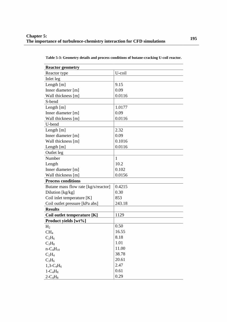
Chapter 5: The importance of turbulence-chemistry interaction for CFD simulations
195
Table 5-3: Geometry details and process conditions of butane-cracking U-coil reactor.
Reactor geometry Reactor type U-coil Inlet leg Length [m] 9.15 Inner diameter [m] 0.09 Wall thickness [m] 0.0116 S-bend Length [m] 1.0177 Inner diameter [m] 0.09 Wall thickness [m] 0.0116 U-bend Length [m] 2.32 Inner diameter [m] 0.09 Wall thickness [m] 0.1016 Length [m] 0.0116 Outlet leg Number 1 Length 10.2 Inner diameter [m] 0.102 Wall thickness [m] 0.0156 Process conditions Butane mass flow rate [kg/s/reactor] 0.4215 Dilution [kg/kg] 0.30 Coil inlet temperature [K] 853 Coil outlet pressure [kPa abs] 243.18 Results Coil outlet temperature [K] 1129 Product yields [wt%] H2 0.50 CH4 16.55 C2H6 8.18 C3H8 1.01 n-C4H10 11.00 C2H4 38.78 C3H6 20.61 1,3-C4H6 2.47 1-C4H8 0.61 2-C4H8 0.29

196 Chapter 5: The importance of turbulence-chemistry interaction for CFD simulations
Figure 5-16: Front view (A), side view (B) and top view (C) of the simulated U-coil.
Figure 5-17 shows the velocity magnitude and the in-plane velocity vectors for six cross sections
in the return bend. The cross sections are labeled from a to f. Note that the in-plane velocity
vectors are not scaled to their magnitude and hence only give the direction of the occurring
secondary flow. Cross section a is located in the straight inlet leg and a fully developed turbulent

Chapter 5: The importance of turbulence-chemistry interaction for CFD simulations
197
flow field is simulated consequently. As the flow enters the S-bend, a low velocity zone is
created near the inner curve of the bend and two counter-rotating vortices prevail. By
introduction to the U-bend, the low-velocity region shifts to the inner curve of the U-coil bend
from c to d. Downstream the U-bend, the two counter-rotating vortices and the dead zone remain
for some length as shown in e and f. The velocity in e and f is also lower compared to the other
cross sections as the inner diameter has enlarged and hence the cross-sectional area is larger. The
effect of these flow patterns have a straightforward effect on temperature and conversion: low
near-wall velocity results in low heat transfer and subsequently in high temperature and high
conversion.
Figure 5-17: Velocity magnitude [m/s] in the six cross sections in the return bend and the location of the cross
sections.
The near-wall low velocity in a U-bend prevails at the inner curve [44-46]. As the U-bend is not
in the plane defined by the inner and outer leg, denoted ‘p1’ in Figure 5-16 C, but rather in the

198 Chapter 5: The importance of turbulence-chemistry interaction for CFD simulations
plane ‘p2’, the near-wall low velocity zone in the outlet leg is not directed towards the inlet leg
but is directed towards the start of the U-bend. Hence, it is in a location receiving a high radiative
heat flux from the furnace walls and burners. Having this zone directed towards the inlet leg
would be beneficial as this is the so-called ‘shadow zone’ receiving less heat flux [47, 48]. Figure
5-18 A, B and C show the velocity, temperature and n-butane yield in plane ‘p1’ shown in Figure
5-16 C in the outlet leg. As shown previously the velocity in the U-bend is higher near the outer
curve of the bend. This results in a low velocity zone near the inner curve of the outlet tube that
remains up to about 3 m in the outer leg. This results in a high temperature near the inner curve of
the outlet leg as shown in Figure 5-18 B. Consequently the n-butane weight fraction in a cross
section of the outlet leg is highly non-uniform.

Chapter 5: The importance of turbulence-chemistry interaction for CFD simulations
199
Figure 5-18: Velocity [m/s] (A), mean temperature [K] (B) and n-butane [wt%] (C) in plane ‘p2’ in the outlet
leg, viz. Figure 5-16 C.
5.5 Conclusions The importance of turbulence-chemistry interaction during steam cracking was assessed. To this
end a code for the three-dimensional simulation of steam cracking reactors based on the free and
open source CFD package OpenFOAM® was developed. The code incorporates the algorithm to
apply the pseudo-steady state assumption to radicals discussed in Chapter 4 and a dynamic
zoning method to speed up the chemistry calculations. The dynamic zoning method can best be
applied per logical core and results in a speed up of the chemistry calculations by a factor of 190
while maintaining a similar accuracy as calculating the chemistry in every cell individually. This

200 Chapter 5: The importance of turbulence-chemistry interaction for CFD simulations
reduction makes the contribution of the chemistry calculations negligible compared to the time
consumed by solving the continuity equations. The effect of turbulent temperature fluctuations is
accounted for by solving an extra continuity equation for temperature variance. Temperature
variance dissipation can be modeled with an algebraic equilibrium model or by solving an extra
continuity equation. Comparison of this approach to DNS data for non-reactive, turbulent pipe
flow showed that the root-mean-square temperature is underpredicted near the wall and
overpredicted in the tube center. Simulation of reactive flow indicated that neglecting the
turbulence-chemistry interaction results in an error on the ethene and propene yields around 0.1-
0.2 wt%. Finally the code was used to simulate butane cracking in an industrial-size U-coil
reactor. Secondary flow patterns in the U-bend were visualized and showed a high temperature,
high conversion zone in the outlet leg near the inner curve of the U-bend which is impossible to
detect with one-dimensional simulations. These detailed simulation results show that this code
can be used for the design and optimization of reactor geometries.

Chapter 5: The importance of turbulence-chemistry interaction for CFD simulations
201
References [1] M. Boileau, G. Staffelbach, B. Cuenot, T. Poinsot, C. Berat, LES of an ignition sequence in a gas turbine engine, Combustion and Flame, 154 (2008) 2-22. [2] L. Esclapez, E. Riber, B. Cuenot, Ignition probability of a partially premixed burner using LES, Proceedings of the Combustion Institute, 35 (2015) 3133-3141. [3] L. Hakim, A. Ruiz, T. Schmitt, M. Boileau, G. Staffelbach, S. Ducruix, B. Cuenot, S. Candel, Large eddy simulations of multiple transcritical coaxial flames submitted to a high-frequency transverse acoustic modulation, Proceedings of the Combustion Institute, 35 (2015) 1461-1468. [4] G. Hannebique, P. Sierra, E. Riber, B. Cuenot, Large Eddy Simulation of Reactive Two-Phase Flow in an Aeronautical Multipoint Burner, Flow Turbulence and Combustion, 90 (2013) 449-469. [5] A. Irannejad, A. Banaeizadeh, F. Jaberi, Large eddy simulation of turbulent spray combustion, Combustion and Flame, 162 (2015) 431-450. [6] W.P. Jones, A.J. Marquis, F. Wang, Large eddy simulation of a premixed propane turbulent bluff body flame using the Eulerian stochastic field method, Fuel, 140 (2015) 514-525. [7] A. Cuoci, A. Frassoldati, A. Stagni, T. Faravelli, E. Ranzi, G. Buzzi-Ferraris, Numerical Modeling of NOx Formation in Turbulent Flames Using a Kinetic Post-processing Technique, Energy & Fuels, 27 (2013) 1104-1122. [8] H. Zimmermann, R. Walzl, Ethylene, in: Ullmann's Encyclopedia of Industrial Chemistry, Wiley-VCH Verlag GmbH & Co. KGaA, 2000. [9] D.R. Chapman, Computational aerodynamics development and outlook, American Institute of Aeronautics and Astronautics Journal, 17 (1979) 1293-1313. [10] H. Choi, P. Moin, Grid-point requirements for large eddy simulation: Chapman's estimates revisited, Physics of Fluids, 24 (2012). [11] J.W. Rogerson, N. Swaminathan, M. Tanahashi, N. Shiwaku, Analysis of progress variable variance equations using DNS data, Third European Combustion Meeting, Chania, Crete, 2007. [12] N. Chakraborty, N. Swaminathan, Effects of Lewis Number on Scalar Variance Transport in Premixed Flames, Flow Turbulence Combust, 87 (2011) 261-292. [13] Y. Pei, E. Hawkes, S. Kook, A Comprehensive Study of Effects of Mixing and Chemical Kinetic Models on Predictions of n-heptane Jet Ignitions with the PDF Method, Flow Turbulence Combust, 91 (2013) 249-280. [14] OpenFOAM - The Open Source CFD Toolbox - User's Guide, OpenCFD Ltd, United Kingdom. [15] OpenFOAM - The Open Source CFD Toolbox - Programmer's Guide, OpenCFD Ltd, United Kingdom. [16] I.R. Gran, B.F. Magnussen, A Numerical Study of a Bluff-Body Stabilized Diffusion Flame. Part 2. Influence of Combustion Modeling And Finite-Rate Chemistry, Combustion Science and Technology, 119 (1996) 191-217. [17] B.F. Magnussen, B.H. Hjertager, On mathematical modeling of turbulent combustion with special emphasis on soot formation and combustion, International Symposium on Combustion, 16 (1977) 719-729. [18] P.J.M. Reid R.C., Poling B.R., Properties of gases and liquids, McGraw-Hill, 1979.

202 Chapter 5: The importance of turbulence-chemistry interaction for CFD simulations
[19] W.H. Green, J.W. Allen, R.W. Ashcraft, G.J. Beran, C.F. Goldsmith, M.R. Harper, A. Jalan, G.R. Magoon, D.M. Matheu, S. Petway, S. Raman, S. Sharma, K.M. Van Geem, J. Song, J. Wen, R.H. West, A. Wong, H.-W. Wong, P.E. Yelvington, Y. J., RMG - Reaction Mechanism Generator v3.3, 2011. [20] C.M. Schietekat, D.J. Van Cauwenberge, K.M. Van Geem, G.B. Marin, Computational fluid dynamics-based design of finned steam cracking reactors, AIChE Journal, 60 (2014) 794-808. [21] R.O. Fox, Computational Models for Turbulent Reacting Flows, Cambridge University Press, Camebridge, UK, 2003. [22] C. Béguier, I. Dekeyser, B.E. Launder, Ratio of scalar and velocity dissipation time scales in shear flow turbulence, Physics of Fluids, 21 (1978) 307-310. [23] J.P.H. Sanders, I. Gokalp, Scalar dissipation rate modelling in variable density turbulent axisymmetric jets and diffusion flames, Physics of Fluids, 10 (1998) 938-948. [24] A. Kossiakoff, F.O. Rice, Thermal Decomposition of Hydrocarbons, Resonance Stabilization and Isomerization of Free Radicals, Journal of the American Chemical Society, 65 (1943) 590-595. [25] F.O. Rice, The Thermal Decomposition of Organic Compounds from the Standpoint of Free Radicals. I. Saturated Hydrocarbons, Journal of the American Chemical Society, 53 (1931) 1959-1972. [26] F.O. Rice, K.F. Herzfeld, The Thermal Decomposition of Organic Compounds from the Standpoint of Free Radicals. VI. The Mechanism of Some Chain Reactions, Journal of the American Chemical Society, 56 (1934) 284-289. [27] R. Van de Vijver, N.M. Vandewiele, P.L. Bhoorasingh, B.L. Slakman, F. Seyedzadeh Khanshan, H.-H. Carstensen, M.-F. Reyniers, G.B. Marin, R.H. West, K.M. Van Geem, Automatic mechanism and kinetic model generation for gas-phase and solution-phase processes: a perspective on best practices, recent advances, and future challenges, International Journal of Chemical Kinetics, submitted (2014). [28] M.K. Sabbe, F. De Vleeschouwer, M.F. Reyniers, M. Waroquier, G.B. Marin, First Principles Based Group Additive Values for the Gas Phase Standard Entropy and Heat Capacity of Hydrocarbons and Hydrocarbon Radicals, J. Phys. Chem. A, 112 (2008) 12235-12251. [29] M.K. Sabbe, M. Saeys, M.F. Reyniers, G.B. Marin, V. Van Speybroeck, M. Waroquier, Group additive values for the gas phase standard enthalpy of formation of hydrocarbons and hydrocarbon radicals, J. Phys. Chem. A, 109 (2005) 7466-7480. [30] F.R. Menter, Two-equation eddy-viscosity turbulence models for engineering applications, Aiaa J., 32 (1994) 1598-1605. [31] H.S. Wilf, Mathematics for the physical sciences, Wiley, 1962. [32] G.H. Golub, J.H. Welsch, Calculation of Gauss quadrature rules, Mathematics of Computation, 23 (1969) 221-&. [33] A. Passalacqua, eigenSolver, 2012. [34] B.S. Garbow, EISPACK — A package of matrix eigensystem routines, Computer Physics Communications, 7 (1974) 179-184. [35] L. Liang, J.G. Stevens, J.T. Farrell, A Dynamic Multi-Zone Partitioning Scheme for Solving Detailed Chemical Kinetics in Reactive Flow Computations, Combustion Science and Technology, 181 (2009) 1345-1371.

Chapter 5: The importance of turbulence-chemistry interaction for CFD simulations
203
[36] F. Perini, High-dimensional, unsupervised cell clustering for computationally efficient engine simulations with detailed combustion chemistry, Fuel, 106 (2013) 344-356. [37] Y. Shi, R.P. Hessel, R.D. Reitz, An adaptive multi-grid chemistry (AMC) model for efficient simulation of HCCI and DI engine combustion, Combustion Theory and Modelling, 13 (2009) 83-104. [38] K.M. Van Geem, M.F. Reyniers, G.B. Marin, Two severity indices for scale-up of steam cracking coils, Industrial & Engineering Chemistry Research, 44 (2005) 3402-3411. [39] L. Redjem-Saad, M. Ould-Rouiss, G. Lauriat, Direct numerical simulation of turbulent heat transfer in pipe flows: Effect of Prandtl number, International Journal of Heat and Fluid Flow, 28 (2007) 847-861. [40] S.V. Patankar, C.H. Liu, E.M. Sparrow, Fully developed flow and heat-transfer in ducts having streamwise-periodic variations of cross-sectional area, Journal of Heat Transfer-Transactions of the Asme, 99 (1977) 180-186. [41] D.J. Van Cauwenberge, C.M. Schietekat, J. Floré, K.M. Van Geem, G.B. Marin, CFD-based design of 3D pyrolysis reactors: RANS vs. LES, Chemical Engineering Journal, accepted (2015). [42] G.R. Newman, B.E. Launder, J.L. Lumley, Modeling the behavior of homogeneous scalar turbulence, Journal of Fluid Mechanics, 111 (1981) 217-232. [43] S.E. Elghobashi, B.E. Launder, Turbulent time scales and the dissipation rate of temperature variance in the thermal mixing layer, Physics of Fluids, 26 (1983) 2415-2419. [44] S.V. Patankar, V.S. Pratap, D.B. Spalding, Prediction of turbulent-flow in curved pipes, Journal of Fluid Mechanics, 67 (1975) 583-595. [45] K. Sudo, M. Sumida, H. Hibara, Experimental investigation on turbulent flow through a circular-sectioned 180 degrees bend, Exp. Fluids, 28 (2000) 51-57. [46] H. Sugiyama, D. Hitomi, Numerical analysis of developing turbulent flow in a 180° bend tube by an algebraic Reynolds stress model, International Journal for Numerical Methods in Fluids, 47 (2005) 1431-1449. [47] G.J. Heynderickx, G.G. Cornelis, G.F. Froment, Circumferential tube skin temperature profiles in thermal cracking coils, AIChE Journal, 38 (1992) 1905-1912. [48] G.J. Heynderickx, G.F. Froment, Simulation and comparison of the run length of an ethane cracking furnace with reactor tubes of circular and elliptical cross sections, Industrial & Engineering Chemistry Research, 37 (1998) 914-922.

204 Chapter 5: The importance of turbulence-chemistry interaction for CFD simulations

Chapter 6: Catalytic coating for reduced coke formation
205
Chapter 6:
Catalytic coating for reduced coke
formation
This chapter has been submitted to Industrial & Engineering Chemistry Research: Carl M. Schietekat, Stamatis Sarris, Larry B. Kool, Wenqing Peng, Patrick Lucas, Kevin M. Van Geem, Guy B. Marin, Catalytic Coating for Reduced Coke Formation in Steam Cracking reactors, submitted

206 Chapter 6: Catalytic coating for reduced coke formation
Abstract A novel catalytic coating that converts coke to carbon oxides by reaction with steam was
developed. Several coating formulations were tested in a jet stirred reactor setup and the best
performing formulation was further evaluated in a pilot plant setup. Application of the coating
during steam cracking of ethane at industrially relevant conditions resulted in a reduction of the
asymptotic coking rate by 76 %. The coating activity remained constant over several
coking/decoking cycles. Scanning electron microscope and energy diffractive X-ray analyses
showed good adhesion of the coating to the base alloy even after several coking/decoking cycles.
Coupled furnace-reactor run length simulations of an industrial ethane cracking unit were
performed and resulted in an increase of the run length by a factor of six. However, the simulated
CO2 yield is higher than the design value of a typical caustic tower.
6.1 Introduction Coke formation on the inner wall of the tubular reactors of steam cracking units has a negative
impact on the economics of the steam cracking process. As coke is formed, the cross-sectional
area of the reactor is reduced, resulting in a higher pressure drop over the reactor. This higher
pressure drop results in a change in product selectivities as bimolecular reactions – often leading
to the formation of aromatics – are favored over monomolecular reactions. Furthermore, the
highly insulative coke layer hampers the heat transfer from the furnace to the reactors. To operate
at a constant cracking severity over time, the fuel flow rate to the furnace burners has to be
increased to compensate for this extra conductive heat transfer resistance. Consequently the
reactor tube metal temperature rises over time. When the maximum tube metal temperature

Chapter 6: Catalytic coating for reduced coke formation
207
(TMT) reaches the metallurgically maximum allowable temperature, typically 1360-1380 K, or
the reactor pressure drop exceeds a predefined maximum value, operation is halted for about 48
hours and the reactors are decoked using steam or - more commonly - a steam/air mixture. As
this decoking operation limits the yearly production capacity and has high operating costs, many
technologies to reduce coke formation have been developed and installed commercially over the
last decades. These technologies can be roughly divided into three groups: three-dimensional
(3D) reactor technologies, feed additives and surface technologies. In 3D reactor technologies,
the reactor tube geometry is altered from the conventional bare, straight tube to a more complex
geometry to enhance convective heat transfer and/or increase heat transfer area. For example
finned tubes [1-3], ribbed [4] or partially ribbed [5] tubes and swirl flow tubes [3] have been
investigated. All these technologies lead to an increased pressure drop compared to conventional
bare tubes and hence affect the ethene selectivity [6]. The second category is one of the most
widely applied techniques to reduce coke formation. For some additives a combination of
pretreatment and continuous addition is applied, while for others only continuous addition is
beneficial. Sulfur-containing compounds are the most commonly applied group of additives [7-
15]. The role of sulfur additives on diminishing carbon monoxide formation is well established,
but their effect on coke formation is debated [16]. Besides sulfur-containing additives,
components with phosphorus [16-18] and silicon [7, 19] have also been investigated. The present
work belongs to the third category of surface technologies such as high performance alloys and
coatings. Steam cracking reactors are typically made out of heat-resistant Fe-Ni-Cr alloys which
resist coke formation by an oxide layer of chromia [20, 21]. Often aluminum and manganese are
added to enhance the coking resistance of the alloys by forming a protective alumina or a

208 Chapter 6: Catalytic coating for reduced coke formation
manganese chromite (MnCr2O4) spinel layer respectively [20, 21]. Alternatively, a thin layer of a
coating can be deposited on the reactor base alloy surface. Distinction can be made between
barrier coatings that passivate the inner wall and catalytic coatings [22] that convert coke to
carbon oxides. A barrier coating pacifies the base alloy by covering the catalytically active sites,
eliminating catalytic coke formation. However, the non-catalytic coke formation through a free-
radical mechanism is not prevented. In contrast, catalytic coatings eliminate the base alloy
catalytic coke formation by covering the original active sites and provide catalytic sites for
converting radically formed coke to carbon oxides and hydrogen by reaction with steam via
gasification reactions. Hence, a positive catalytic activity is added besides the elimination of the
negative catalytic activity of the base alloy.
Several authors have investigated the application of barrier coatings in steam cracking reactors.
Zychlinski et al. [23] tested the performance of the AlcroPlex® coating in an electrobalance setup.
AlcroPlex® is an Al/Si barrier coating that is applied in a two-step chemical vapor deposition
process. This coating decreases the total coke deposition up to 90 % when cracking ethane and up
to 80 % when cracking naphtha compared to a reference HP 40 material. Ganser et al. [24]
described the application of AlcroPlex® in an industrial ethane cracker. The run length of the
furnace was doubled from 30 days to more than 60 days after installation of coated tubes. In
addition, lower CO formation was measured and decoking operation was accomplished in less
than half the normal time. After one year of installation, metallurgical analyses were performed
on the coated reactor tubes. No carburization of the tubes was seen and the coating seemed
essentially unchanged.

Chapter 6: Catalytic coating for reduced coke formation
209
NOVA Chemicals and Kubota have developed a technology - commercialized as ANK 400 - to
reduce both catalytically and radically formed coke [25, 26]. The heat resistant base alloy is
separated from the process gas with a micron-sized inert manganese chromium oxide ANK 400
spinel. Application of fresh ANK 400 tubes in two ethane cracking furnaces resulted in an
increase of the run length from 33 to more than 400 days. Subsequent runs had a duration of
around 175 days. Westaim Surface Engineered Products developed another barrier coating, called
CoatAlloy [27-29]. CoatAlloy consists of an engineered surface, an enrichment pool and
diffusion barriers coated on the bulk alloy. In the original patent [30], the intermediary diffusion
barrier is an aluminum-containing coating deposited directly onto the bulk alloy substrate prior to
deposition of the enrichment pool. The enrichment pool is a MCrAlX material in which M is
nickel, cobalt, iron or a mixture thereof and X is yttrium, hafnium, zirconium, lanthanum or a
combination thereof. This enrichment pool and the bulk alloy are heat-treated to metallurgically
bond the coating and to form a multiphasic microstructure. The overlay coating is then
aluminized by depositing a layer of aluminum and oxidizing the resulting coating to form an
alumina surface layer. Between 1995 and 2001 several improvements have been made to the
technology resulting in an increased operating limit from 1293 K (Original CoatAlloyTM) to 1333
K (CoatAlloyTM - 1060) and 1373 K (CoatAlloyTM - 1100) [29]. By 2001, CoatAlloy coatings
were installed in 25 furnaces globally and typically resulted in a decrease in coking rate by about
90 % [29].
Besides the inert barrier coatings, several catalytic coatings have also been developed. The so-
called Catalyzed-Assisted Manufacture of Olefins (CAMOL) coating was developed by

210 Chapter 6: Catalytic coating for reduced coke formation
Quantiam Technologies and NOVA Chemicals from 2001 to 2008 and is since 2011
commercialized by BASF Qtech [22, 31]. Two families of coatings have been developed; one
manganese and one tungsten based [32]. As such two products are commercially available: the
Low-Catalytic Gasifier (LCG) and the High-Catalytic Gasifier (HCG) [33]. The LCG can be used
for ethane-propane cracking, while the HCG coating targets at heavier feedstocks cracking such
as naphthas. The coatings have been installed in an industrial naphtha cracking furnace. After
three years in operation, it was found that modified start up procedures are required in order to
reactivate the catalytic sites [33]. A small amount of HCG was coated on the reactors’ outlet
tubes. Before application of the coating, the furnace was typically limited by high outlet TMT’s.
However, with the help of this small amount of HCG, the furnace became pressure drop limited
instead [33]. This shows that only a small amount of HCG can gasify a significant amount of
coke. A sample taken from a reactor after 14 months of service showed minor damage to the
coating which could be repaired after an oxidation procedure [33].
SK-corporation developed a method of on-line coating the reactor inner walls with a catalytic
film, called PY-COAT [34]. The method comprises three steps of vapor depositing: a solution of
a metal alkoxide and a chromic compound to form a buffer layer on the inner walls; a metal
alkoxide as a barrier on the buffer layer and finally an alkali metal/alkaline earth metal compound
alone or mixed with metal alkoxides as a decoking layer on the barrier. Application in a
Millisecond naphtha cracking furnace more than doubled the run length.
In the following, a new catalytic coating, called YieldUp, is presented. The coating is based upon
a family of ceramic catalysts having doped perovskite structures that are capable of converting
coke to carbon oxides and hydrogen. The performance of different formulations of this coating

Chapter 6: Catalytic coating for reduced coke formation 211
was probed in a jet stirred reactor (JSR) setup. The optimal coating formulation was further tested
in a pilot plant setup. Finally, the application of the coating when scaling the JSR and pilot plant
data to an industrial ethane cracker w as simulated.
6.2 Experimental section
Coating 6.2.1
YieldUp consists of an engineered synthetic ceramic [35, 36]. When exposed to high temperature
steam, water molecules are chemisorbed and deprotonated, resulting in the formation of highly
reactive oxygen atoms that react with deposited coke to carbon oxides. A family of YieldUp
catalyst materials has been developed that provides a wide range of anti-coking activities as
described below. The ceramic coating was applied to the JSR coupons by forming an aqueous
slurry of catalyst microparticles and other additives and dip-coating the coupons, followed by a
high-temperature sintering step. The same slurry formulation was used to coat the inner surface
of the reactor tubes used in the pilot plant experiments. A typical coating thickness ranges from
20 to 50 µm.
Jet stirred reactor 6.2.2
As the jet stirred reactor setup has been extensively described by Muñoz Gandarillas et al. [20,
21], only a brief description is given here. The setup consists out of three parts: a feed section, a
reactor section and an analysis section. The feed section controls the mass flow rates of gases and
water by thermal mass flow controllers, vaporizes water to steam in an evaporator, mixes the
steam with the hydrocarbon feedstock and heats the mixture to the reactor inlet temperature of
903 K. The reaction section is a jet stirred reactor made out of quartz. Inside the reactor, a small,
212 Chapter 6: Catalytic coating for reduced coke formation
flat coupon is suspended from an electrobalance. The coupon mass is tracked over time and
increases as coke deposits on the coupon. In the analysis section, the reactor effluent is first
quenched to prevent further cracking. Afterwards, the reactor effluent composition is measured
with two gas chromatographs (GC) using nitrogen as internal standard: a refinery gas analyzer
dedicated to the analysis of components with less than 5 carbon atoms and a TRACETM Ultra GC
detecting hydrocarbons ranging from methane to naphthalene.
Experimental procedures and conditions in the jet stirred 6.2.3reactor
Similar operating procedures and conditions were used as described by Muñoz Gandarillas et al.
[20] and hence, only a brief description is given here. The experiments consisted of three cycles
of a 6 h cracking step and a decoking step and one cycle of a 12 h pre-oxidation step and a 2 h
cracking step. Afterwards, the coupons were removed for Scanning electron microscope (SEM)
and energy dispersive X-ray (EDX) analyses. Before the first cycle, a pre-oxidation step is
performed. In the pre-oxidation step, the coupon is oxidized in the reactor to have a surface state
similar to the start-of-run surface state of an industrial reactor. First, the reactor temperature is
raised from room temperature to 1023 K under a constant 6.7 · 10-3 Nl s-1 nitrogen flow.
Afterwards, the feed is switched to air to oxidize the coupon. No presulfidation of the coupon
was performed. After 12 h of oxidation, the feed is switched back to nitrogen and the reactor
temperature is increased to 1283 K. During heating, 11.0 · 10-6 kg s-1 of a water/dimethyl
disulfide (DMDS) solution and 0.0275 Nl s-1 ethane are send to the evaporators and vented in
order to get a steady evaporation and mixing. DMDS was dissolved in water to have a continuous
addition of 50 · 10-6 kg DMDS/kg ethane which is common practice in industrial crackers to limit

Chapter 6: Catalytic coating for reduced coke formation 213
the formation of carbon oxides. Once the set reactor temperature is reached, the cracking mixture
is sent to the reactor. The reactor temperature is controlled throughout the cracking runs at 1159
K, a value that is reached 5 min after introduction of the cracking mixture in the reactor. After the
6 or 2 h of cracking, the reactor temperature is set to 1173 K and the flow rate of ethane and
steam is set to zero, leaving only nitrogen to purge the reactor. Once this temperature is reached,
the reactor is cooled down to 1023 K with a steam flow rate of 6.7 · 10-6 kg s-1. Once that
temperature is reached, a mixture of air (8.3 · 10-3 Nl/s) and nitrogen (8.3 · 10-3 Nl/s) is fed to the
reactor. During the decoking step, the reactor is heated to 1173 K using a heating ramp of 300
K/h. As soon as the reactor reaches 1173 K, the air flow is maintained, but the nitrogen flow is
switched off to mimic industrial decoking practice. These conditions are kept for 15 minutes and
then the feed to the reactor is switched back to nitrogen (6.7·10-3 Nl/s) only. In the fourth cycle,
i.e. after 2 h of cracking, the coupon was not decoked, but removed from the reactor for analysis
after cooling down the reactor to room temperature with a nitrogen flow rate of 6.7·10-3 Nl/s.
Pilot plant setup 6.2.4
A schematic representation of the pilot plant is shown in Figure 6-1. Since the main parts of this
unit, the analytical equipment and the calibration procedure have been described previously by
Wang et al. [8], Dhuyvetter et al. [10] Van Geem et al. [37], Pyl et al. [38, 39] and Dijkmans et
al. [40] , only a short description is given here. Similar to the JSR setup, the pilot plant setup has
three main sections; the feed section, the reaction section and the analysis section. In the feed
section, the flow rate of the different feedstocks to the reactor is controlled by CORI-FLOW®
pumps. Ethane, air and nitrogen are fed directly from the gas bottle, while demineralized water is
fed from an intermediate storage vessel. The reactor is mounted in a furnace of about 4 m long,

214 Chapter 6: Catalytic coating for reduced coke formation
0.7 m wide and 2.6 m high. The furnace is wall fired with ninety premixed gas burners
distributed over the two side walls. The furnace is divided into seven separate cells by means of
brick walls inside the furnace. The seven cells can be fired independently to set a temperature
profile along the reactor axial coordinate. Twenty thermocouples and eight manometers along the
reactor measure the temperature and pressure of the process gas. The reaction section of the
reactor tube, i.e. where the process gas temperature is above 823 K, is about 12 m long and has an
internal diameter of 9 mm. Just downstream the furnace, a sample is taken for the on-line C5+
analysis. Next, the effluent is cooled in a double pipe heat exchanger using oil as coolant. The
condensate and tars are removed from the oil cooler effluent with a knock-out vessel and a
cyclone. A fraction of the gaseous effluent of the cyclone is withdrawn for on-line C4- analysis,
while the rest is sent directly to the flare. Nitrogen is added before the C4- analysis to be used as
internal standard. The reactor outlet pressure is regulated by a control valve. As steam is not
measured on any gas chromatograph and as it cannot be considered an inert because of the high
carbon oxides and hydrogen yields, normalization was performed based on the carbon balance
instead of the total mass balance.

Chapter 6: Catalytic coating for reduced coke formation 215
Figure 6-1: Schematic overview [37] of the pilot plant setup indicating the process gas temperature (○),
reactor outer wall temperature (●) and process gas pressure (P) measurements (1: Mass flow controllers, 2:
demineralized water reservoir, 3: gas bottles, 4: sampling oven at 300°C, 5: heated transfer lines at 300°C, 6:
oil cooled heat exchanger, 7: water cooled condenser, 8: cyclone, 9: nitrogen internal standard addition, 10:
outlet pressure control valve, 11: water cooled heat exchanger, 12: gypsum dryer).
Experimental procedures and conditions in the pilot plant 6.2.5setup
The experiments carried out in the pilot plant consisted of the same three main steps as the JSR
experiments; pre-oxidation, cracking and decoking. The process conditions of all three step are
summarized in Table 6-1. Prior to a cracking experiment, the reactor was pre-oxidized with a
steam/air mixture. After 2 hours of pre-oxidation, nitrogen is fed to the reactor and the desired
cracking temperature profile is set. Once the temperature profile is reached, the flow rates of
steam, ethane and nitrogen are set. Upon the introduction of hydrocarbons, the process gas

216 Chapter 6: Catalytic coating for reduced coke formation
temperature decreases by about 20 K due to the endothermic cracking reactions. After about 20
minutes the set temperature profile is again reached. In the experiments where continuous DMDS
addition was applied, the DMDS was added in the water feed barrel to provide the desired
concentration. The tubing connecting the water barrel to the reactor was treated with Restek’s
Sulfinert® coating to avoid adsorption of DMDS on the tubing inner walls. After 6 hours of
cracking, the flow rate of the cracking mixture is set to zero, nitrogen is fed to the reactor and the
temperatures of cell 4 to 7 are set to 1023 K. Once this new temperature profile is reached, a
steam/air mixture is used to decoke the reactor. During decoking, the CO and CO2 concentrations
in the reactor effluent are continuously measured by means of an infrared meter. From these
values and the measured effluent flow rate, the coke burned from the reactor wall is determined.
When the molar CO2 concentration of the effluent drops below 1 mol %, the temperatures of cell
4 to 7 are increased to 1073 K. When the concentration of CO2 in the effluent is lower than 0.1
mol %, the nitrogen flow is stopped and only air is used. Furthermore, a filter is installed in the
condensers after the reactor, where entrained coke is collected. After each experiment, this
collected coke is dried and weighed. The reported coke values are the sum of burned and
entrained coke. In total six pilot plant experiments were performed, referred to as INC, YieldUp,
NO S, PRES, DIL1 and DIL2. In the INC experiment an uncoated Incoloy 800HT reactor was
used. In all other experiments, the inner wall of the reactor was coated with YieldUp1 from cell 3
to 7 as indicated by the red, dashed line in Figure 6-1. Although the same temperature profile
shown in Table 6-1 was used in all experiments, the mass flow rates were altered to study the
effect of dilution and DMDS addition on the coating performance. The process conditions of all
experiments are summarized in Table 6-3. INC and YieldUp serve as the reference cases using an
Chapter 6: Catalytic coating for reduced coke formation
217
uncoated and coated reactor respectively. In these experiments, ethane was cracked at a flow rate
of 8.333·10-4 kg/s, a steam dilution of 0.385 kg steam/kg ethane and a continuous sulfur addition
of 50·10-6 kg DMDS/kg ethane. In experiment NO S, the effect of DMDS addition was tested by
not adding any DMDS. It is noted that this experiment was performed first not to influence the
results by the memory effect of sulfur on the coil from previous experiments as reported by Tong
et al. [41]. In experiment PRES, the effect of DMDS presulfiding was assessed. Presulfiding was
performed after pre-oxidation using a 750·10-6 kg DMDS/kg water mixture at a flow rate of
1.111·10-3 kg/s for 1 hour. In DIL1, the effect of lower steam partial pressure was investigated.
The steam mass flow rate was halved to 0.161·10-3 kg/s and nitrogen was added to provide the
same molar dilution. In DIL2, the effect of lower total dilution was investigated by reducing the
dilution to 0.1925 kg steam/kg ethane. To maintain the same total molar inlet flow rate, the
ethane and steam flow rate were scaled to 1.036·10-3 and 0.199·10-3 kg/s respectively.

218 Chapter 6: Catalytic coating for reduced coke formation
Table 6-1: Process conditions of the pre-oxidation, pre-sulfidation, cracking and decoking step during a pilot plant experiment.
Pre-oxidation Pre-sulfidation Cracking Decoking
Pre-start Start Pre-start Start* Pre-start Start CO2<1vol% CO2<0.1vol%
Mass flow rate [g/s]
Steam 0.278 1.111 1.111 0.0 0.321 0.280 0.280 0.280 0.0
Air 0.278 0.0 0.0 0.0 0.0 0.0 0.230 0.230 0.230
Ethane 0.0 0.0 0.0 0.0 0.833 0.0 0.0 0.0 0.0
Nitrogen 0.0 0.0 0.0 0.833 0.0 0.230 0.0 0.0 0.0
Dimethyl disulfide 0.0 0.0 8.333·10-4 0.0 4.165·10-5 0.0 0.0 0.0 0.0
Temperature profile [K]
COT cell 1 773 773 773 773 773 773 773
COT cell 2 823 773 823 823 823 823 823
COT cell 3 1073 903 1023 1023 1023 1023 1023
COT cell 4 1073 1023 1063 1073 1073 1123 1123
COT cell 5 1073 1093 1093 1073 1073 1123 1123
COT cell 6 1073 1133 1113 1073 1073 1123 1123
COT cell 7 1073 1143 1128 1073 1073 1123 1123
*Flow rates of YieldUp and INC experiment, for other experiments see Table 6-3.

Chapter 6: Catalytic coating for reduced coke formation 219
6.3 Experimental results and discussion
Jet stirred reactor 6.3.1
6.3.1.1 Product yields and coking rates
The effect of applying the YieldUp catalytic coating on product yields and coke formation was
assessed in the JSR setup. To this end three coupons coated with a different YieldUp formulation
were tested and compared to a reference Incoloy 800HT coupon. The process conditions, product
yields and coking results are shown in Table 6-2. The conversion of ethane amounted to about 70
wt% and the yields of ethene and propene were about 50.5 wt% and 0.78 wt% respectively. The
yields of hydrogen and carbon oxides increased by application of the YieldUp1 formulation. The
yields of other components are not influenced by the coating as differences are within the
experimental error. The amount of coke deposited on the coupon was significantly decreased in
all cycles by application of all coating formulations compared to the reference Incoloy 800HT
alloy. For the first cycle coke reductions of 87, 74 and 73 % were obtained compared to the
Incoloy 800HT alloy for the YieldUp1, YieldUp2 and YieldUp3 formulation respectively. The
lower amount of deposited coke results in higher carbon oxides and hydrogen yields in the
YieldUp1 experiment as part of the coke formed on the coating is gasified. This holds to a lesser
extent for YieldUp2 and YieldUp3 as for these coating formulations less coke if gasified.

220 Chapter 6: Catalytic coating for reduced coke formation
Table 6-2: Process conditions, product yields and coking results of ethane cracking in the JSR.
Coupons Incoloy 800HT YieldUp1 YieldUp2 YieldUp3
Temperature [K] 1159 1159 1159 1159 Ethane flow rate [kg/s] 3.63 · 10-6 3.63 · 10-6 3.63 · 10-6 3.63 · 10-6 Steam flow rate [kg/s] 11.0 · 10-6 11.0 · 10-6 11.0 · 10-6 11.0 · 10-6 Dilution [kg/kg] 0.33 0.33 0.33 0.33 Conversion [wt%] 69.34 70.33 69.44 69.47
Mass of coke [10-6 kg / 6h]
1st cycle 39.0 5.0 10.0 10.2 2nd cycle 42.5 6.5 12.0 11.3 3rd cycle 45.0 9.0 17.2 12.6
Rc,init. [10-6 kg /s/m²]
1st cycle 22.4 2.0 5.3 5.8
2nd cycle 19.2 2.3 7.2 5.80
3rd cycle 19.1 2.4 10.2 7.70
4th cycle 19.10 4.1 5.3 5.20
Rc,asym. [10-6 kg/s/m²]
1st cycle 4.0 0.9 1.0 1.1
2nd cycle 6.1 1.2 1.9 1.5
3rd cycle 7.0 1.7 2.2 1.8
Product Yields [wt% dry]*
H2 4.28 4.37 4.22 4.21
CO 0.05 0.93 0.07 0.06
CO2 0.02 0.19 0.02 0.02
CH4 7.06 7.12 7.18 7.1
C2H6 30.66 29.67 30.56 30.53
C2H4 50.53 50.64 50.67 50.53
C3H8 0.11 0.11 0.12 0.11
C3H6 0.75 0.78 0.81 0.80
C2H2 1.28 1.41 1.41 1.46
1,3-C4H6 1.11 1.13 1.03 1.03
Benzene 2.42 2.37 2.34 2.33 * Product yields averaged over all cycles. Asymptotic carbon oxides and hydrogen yields reported.

Chapter 6: Catalytic coating for reduced coke formation
221
The total amount of coke deposited in these 6 hours experiments depends on the respective
contribution of the initial, catalytic coke formation rate and the asymptotic, free-radical coke
formation rate. However, in industrial units the run length is almost solely determined by the
asymptotic coke formation rate. The initial and asymptotic coking rates are depicted in Figure
6-2A and B respectively. The initial coking rate is calculated as the average coking rate between
minute 15 and 30 of the cracking experiment. The first 15 min are excluded because the mass
signal has to stabilize after the introduction of the cracking mixture in the reactor. The asymptotic
coke formation rate is calculated as the average coking rate over the last cracking hour, when the
rate stays constant over time. As the fourth cracking run only lasted 2 h, no asymptotic coking
rate is reported for this cycle. The initial coking rates of all YieldUp formulations are
significantly lower than for the reference Incoloy 800HT alloy. YieldUp1 performs best, while
YieldUp2 and YieldUp3 show a similar initial coking rate. The initial coking rates of the coated
coupons remain more or less stable over subsequent cycles, besides a small increase in the third
cycle for YieldUp2 and YieldUp3. Also in the asymptotic regime, application of any of the tested
YieldUp formulations is seen to reduce the coking rate. Again the YieldUp1 formulation has the
best performance, showing a reduction of the asymptotic coking rate by 73, 75 and 74 %
compared to the reference coupon for the 1st, 2nd and 3rd cycle respectively. This stable reduction
in coking rate over multiple cycles shows that the coating retains its catalytic activity over
different coking/decoking cycles.

222 Chapter 6: Catalytic coating for reduced coke formation
Figure 6-2: Initial coking rate [10-6 kg/m²/s] (A) and asymptotic coking rate [10-6 kg/m²/s] (B) as a function of
coking cycle [-]: - Incoloy 800HT; - YieldUp1; - YieldUp2; - YieldUp3.

Chapter 6: Catalytic coating for reduced coke formation
223
6.3.1.2 SEM and EDX analyses
Scanning electron microscope (SEM) analysis of the top surface and cross-sectional energy
dispersive X-ray (EDX) line scans and element mappings have been performed on the coked
coupons after the 4th coking cycle. All analyses were performed as described by Muñoz
Gandarillas et al.[20].
A top view of the coked YieldUp1, YieldUp2 and YieldUp3 coupon after the fourth cycle of
ethane cracking is shown in Figure 6-3A, B and C respectively. Multiple cracks are seen in the
surface of the YieldUp1 coupon. This coupon had the least amount of coke deposited after 2
hours of cracking. Hence, the surface morphology of the coked sample retains many
characteristics of the catalytic coating underneath because of the low coke deposition. The
surface of the YieldUp2 coupon looks distinctly different with a clear coke layer covering the
coating. The YieldUp3 surface shows characteristics of both YieldUp1 and YieldUp2. The
amount of coke deposited is also intermediary between the two other coatings. The surface
exhibits some cracks in the coke layer, fewer in number, but larger than in the YieldUp1 sample.

224 Chapter 6: Catalytic coating for reduced coke formation
Figure 6-3: SEM images of coked surface after the fourth cracking cycle: 750×, 10 kV of: YieldUp1 (A),
YieldUp2 (B) and YieldUp3 (C).
Cross-sectional cuts were made of all three coked, coated coupons and investigated with SEM,
EDX line scans and elemental mappings. The cross-sectional SEM images of the three coupons
are shown in Figure 6-4. Five segments can be distinguished in all three coupons; the bulk alloy,
an oxide layer, the catalytic coating, the coke layer and the resin embedment used during the
analysis. The oxide layer was partly present before dip-coating the coupons, but also stems from
the sintering step in the manufacturing process. This step aims at increasing the adhesion of the
coating to the alloy by allowing atoms to diffuse between the layers at high temperature.

Chapter 6: Catalytic coating for reduced coke formation
225
Figure 6-4: Cross sections of coked coupons of YieldUp1 (A), YieldUp2 (B) and YieldUp3 (C), arrows indicate
path of EDX line scan analyses.
From Figure 6-4, the thickness and structure of the different layers can be analyzed. The
YieldUp1 coating is approximately 15 µm thick and is very porous. This high surface area
explains its superior activity compared to the two other coating formulations. The thickness of the
oxide layer varies between 2 and 8 µm. The coke layer thickness is below 1 µm. No clear voids
are seen in-between the coating, the oxide layer and the base alloy. This indicates the good
adhesion between the different layers after several coking/decoking cycles and even after the
thermal stresses from cooling down the coupon to room temperature. The YieldUp2 coating is 30
µm thick. The coating is less porous than YieldUp1, which can explain the lower coke
gasification activity. Again the different layers are still well attached showing the stable adhesion
of the coating on the bulk alloy. The oxide layer of YieldUp2 is significantly thinner, only about
2-4 µm. The thickness of the catalytic layer of YieldUp3 is about 25 µm. Some dense particles
can be seen in this layer surrounded by a more porous phase. Two large cracks are seen in the
catalytic layer. The left crack almost reaches the oxide layer and spalling of the coating seems
imminent after more cycles. As the YieldUp3 formulation was made using a different method

226 Chapter 6: Catalytic coating for reduced coke formation
than YieldUp1 and YieldUp2, this method seems inferior concerning coating adhesion. The oxide
layer is similar to the layer on YieldUp2, i.e. about 2-4 µm thick.
The arrows in Figure 6-4 indicate the path of the EDX line scans. The line scan results are shown
in Figure 6-5, Figure 6-6 and Figure 6-7 for YieldUp1, YieldUp2 and YieldUp3 respectively. The
line scans clearly show the coating elements, i.e. barium, cerium, zirconium and oxygen, in the
coating layer. The oxide layer shows some typical features of an high-alloyed centrifugal cast Ni-
Cr-Fe alloy: a high presence of chromium, manganese and oxygen indicating a MnCr2O4-spinel,
the presence of Si, indicating SiO2 and an overall low presence of iron and nickel. The oxide
layer also contains elements of the coating which assures a good adhesion between the coating
and the oxide layer. The presence of sulfur was assessed because of the continuous addition of
DMDS during cracking, but the sulfur content was found to be negligible and is therefore not
shown. In all coupons, negligible presence of nickel and iron is found in the catalytic coating,
showing that the oxide layer works as an efficient diffusion barrier for these elements.

Chapter 6: Catalytic coating for reduced coke formation
227
Figure 6-5: EDX line scan analysis of coked YieldUp1 coupon at 15 kV: coating elements (top): - O;
- Ba; - Ce; - Zr; and base alloy elements (bottom): - O; - Cr; -
Mn; - Si; - Ni; - Fe.

228 Chapter 6: Catalytic coating for reduced coke formation
Figure 6-6: EDX line scan analysis of coked YieldUp2 coupon at 15 kV: coating elements (top): - O;
- Ba; - Ce; - Zr; and base alloy elements (bottom): - O; - Cr; -
Mn; - Si; - Ni; -Fe.

Chapter 6: Catalytic coating for reduced coke formation
229
Figure 6-7: EDX line scan analysis of coked YieldUp3 coupon at 15 kV: coating elements (top): - O;
- Ba; - Ce; - Zr; and base alloy elements (bottom): - O; - Cr; -
Mn; - Si; - Ni; - Fe.
The elemental mappings of all three coupons are shown in Figure 6-8. The element mappings of
YieldUp1 in Figure 6-8 show that barium, cerium and oxygen are uniformly distributed over the
coating, while agglomerates of high zirconium concentration exist. Some carbon is present in the
coating pores showing that the entire surface area of the coating is used for coke gasification. The

230 Chapter 6: Catalytic coating for reduced coke formation
oxygen and chromium mappings show that the oxide layer covers the base alloy fully. The oxide
layer acts as a good diffusion barrier as no iron and nickel are detected above the oxide layer. In
the YieldUp2 formulation, more zirconium was used as also seen in the elemental mappings.
Both barium and zirconium are quite uniformly dispersed over the layer, while local spots with
high cerium concentration exist. The presence of carbon is lower due to the lower porosity of the
coating compared to YieldUp1. Although the oxide layer is much thinner than the YieldUp1
coating, it fully covers the base alloy and prevents nickel and iron from diffusing upwards. From
the zirconium mapping, it is seen that the dense phase of the YieldUp3 coating mainly consists of
zirconium and lacks cerium. Again the cracks and pores are filled with carbon. The oxide layer is
less continuous than with YieldUp1 and YieldUp2 as some interruptions of low oxygen content
exist. Nonetheless, low iron and nickel presence is detected above the oxide layer.

Chapter 6: Catalytic coating for reduced coke formation 231
Figure 6-8: Element mappings of cross sections of coked coupons of YieldUp1 (top), YieldUp2 (middle) and
YieldUp3 (bottom).
Pilot plant setup 6.3.2
As YieldUp1 showed the best coking resistance and a good adhesion to the base alloy during the
JSR experiments, this formulation was further tested in a pilot plant setup for steam cracking. As
depicted in Figure 6-1, the YieldUp1 coating was applied on the reactor inner wall from cell 3 to
cell 7. Six experiments were performed evaluating the effect of sulfur addition and dilution on
coking rate and product yields. The results of the pilot experiments are summarized in Table 6-3.

232 Chapter 6: Catalytic coating for reduced coke formation
Table 6-3: Summary of coke and yield data of pilot plant ethane experiments.
Experiment INC YieldUp1 NO S PRES DIL1 DIL2
Process conditions
Reactor Incoloy YieldUp1 YieldUp1 YieldUp1 YieldUp1 YieldUp1
Feed [10-3 kg/s] 0.833 0.833 0.833 0.833 0.833 1.036
H2O flow rate [10-3 kg/s] 0.321 0.321 0.321 0.321 0.161 0.199
N2 flow rate [10-3 kg/s] 0.000 0.000 0.000 0.000 0.249 0.000
S addition [10-6 kg S/ kg ethane] 50 50 0 50 50 50
H2O/HC ratio [10-3 kg/s] 0.385 0.385 0.385 0.385 0.193 0.193
(H2O+N2)/ethane ratio [kg/kg] 0.385 0.385 0.385 0.385 0.492 0.193
(H2O+N2)/ethane ratio [mol/mol] 0.642 0.642 0.642 0.642 0.642 0.321
COT [K] 1128.15 1128.15 1128.15 1128.15 1128.15 1128.15
COP [bar abs] 1.7 1.7 1.7 1.7 1.7 1.7
Yields*
∑C4- [wt%] 98.9 102.4 104.7 102.6 101.2 100.8
Ethene selectivity [wt%/wt%] 80.3 80.0 78.2 79.7 79.8 80.1
Ethane conversion [wt%] 63.9 63.2 63.9 64.0 63.4 61.5
H2 4.20 4.54 4.88 4.52 4.24 4.04
CH4 3.72 3.48 3.65 3.58 3.67 3.59
C2H6 36.10 36.79 36.13 35.98 36.62 38.50
C2H4 51.33 50.57 49.97 51.03 50.55 49.26
1,3-C4H6 1.40 1.31 1.20 1.33 1.41 1.38
CO 0.01 1.75 3.72 2.03 1.65 0.99
CO2 0.02 2.19 3.61 2.44 1.02 0.98
Net coke deposited [g coke/6h] 18.5 4.4 2.1 3.3 3.9 6.1
Gasified coke [g C/6h] 1.8 242.4 464.3 276.9 177.5 154.8
% C to coke and COx [%] 0.02 3.37 6.45 3.85 2.46 1.73
* Average over 9-13 effluent analyses per experiment. Asymptotic carbon oxides and hydrogen yields reported.

Chapter 6: Catalytic coating for reduced coke formation
233
Comparing experiment INC and YieldUp1, it is seen that the amount of coke deposited was
reduced 76 % by application of the YieldUp1 coating compared to the Incoloy 800HT reactor.
This value corresponds well to the measured decrease of the asymptotic coking rate during the
JSR experiments. Consequently, the effluent contained more hydrogen, CO and CO2 than during
the INC experiment as more coke was gasified. The increase in hydrogen and carbon oxide yields
by application of the YieldUp1 coating is much higher in the pilot plant experiments than in the
JSR experiments due to the higher surface-to-volume ratio of the pilot plant reactor: 5.1 m-1 and
444.4 m-1 for the JSR and pilot reactor respectively. Taking into account the small difference in
conversion between the INC and YieldUp1 experiment and the experimental errors, the yield of
other components is not significantly influenced by the coating. From the carbon oxides yields,
the amount of coke gasified by the coating can be calculated. As seen from Table 6-3, 1.8 g of
coke is gasified in the INC reference experiment, while 242.4 g of coke is gasified in the
YieldUp1 experiment. Hence, 0.02 and 3.37 % of all carbon fed to the reactor is converted to
coke or carbon oxides in the INC and YieldUp1 experiment respectively. This consideration
shows that the coating gasifies more than the amount of coke that is normally formed on a
reference alloy. This could be caused by the high surface roughness of the coating resulting in a
higher coke deposition rate or the coating converting gaseous hydrocarbons to carbon oxides. It is
clear that this coating formulation is too active and that more research is needed into tuning the
coating activity.
The absence of continuous DMDS addition was evaluated in experiment NO S. The influence on
hydrocarbon species yields is minor. The increase in CO and CO2 yield is much more apparent;

234 Chapter 6: Catalytic coating for reduced coke formation
CO increases from 1.8 to 3.7 wt% and CO2 from 2.2 to 3.6 wt% compared to experiment
YieldUp1. Hence, continuous DMDS addition can mitigate CO and CO2 production when the
coating is applied. In agreement with previous works [8, 9], the coking rate decreased without the
addition of DMDS. Presulfidization of the coil with a steam/DMDS solution prior to the
continuous DMDS addition was evaluated in experiment PRES. Presulfidization before
continuous DMDS addition shows a coke tendency that is slightly higher than to solely
continuous DMDS addition, resulting in lower carbon oxides yields. Finally, the effect of
lowering the dilution was evaluated in two experiments: DIL1 and DIL2. In experiment DIL1 the
steam mass flow rate was halved and nitrogen was added to remain at the same total molar flow
rate to cancel out the effect of reduced hydrocarbon partial pressure on the product yields. As
DMDS was continuously added, comparison is made to the YieldUp1 experiment. The yields of
CO and CO2 were lower; CO dropped from 1.8 to 1.7 wt% and CO2 from 2.4 to 1.0 wt%. The
low dilution experiment DIL1 shows a coking rate similar to YieldUp1. Hence, it seems enough
water is present to convert coke to carbon oxides as in experiment YieldUp1. In experiment DIL2
the steam dilution was also halved to 0.1925 g steam/g ethane. However, no nitrogen was added
in this experiment. To maintain a similar conversion, the flow rates of ethane and steam were
scaled to have the same molar flow rate as in experiment YieldUp1. Lower ethane conversion
and resulting lower olefin yields were measured. The CO and CO2 yields decreased to 0.99 and
0.98 wt% respectively. In experiment DIL2 a higher coking rate was measured compared to
YieldUp1. Higher coke formation is expected due to higher hydrocarbons partial pressure and the
coating converting less coke to CO and CO2 due to the lower steam partial pressure. However,
comparing with the INC experiment, a decrease in coking rate by 67 % is still obtained while

Chapter 6: Catalytic coating for reduced coke formation 235
increasing the ethane throughput by 24 %. This experiment shows that besides obtaining longer
run lengths, also higher production capacity can be obtained by application of the coating.
6.4 Simulation of an industrial ethane steam cracking unit
Furnace and reactor model 6.4.1
The reactor simulations were performed using the in-house developed COILSIM1D program.
This program applies the plug flow assumption and solves the resulting one-dimensional
continuity, momentum and energy equations. As COILSIM1D has been described in detail by
Van Geem et al. [42] and Pyl et al. [38], only the modifications made to model the effect of the
coating on product yields and coking rate are discussed here.
As by application of the coating the hydrogen and carbon oxides yields are strongly influenced,
the effect of coking and gasification reactions on the product yields is explicitly modeled. The net
amount of coke deposited depends on two terms; coke formation and subsequent coke
gasification. Coke formation is modeled using the coke model of Plehiers [43] which uses ethene
and propene as coke precursors. Gasification was modeled using the following reactions:
� � ��� → �� � ��
� � 2��� → ��� � 2�� Two sets of Arrhenius parameters for the gas-solid reactions were used to model the coated and
the uncoated reactor respectively. For the uncoated reactor case, the original model parameters of
the model of Plehiers were used. The activation energy of the gasification reactions was taken

236 Chapter 6: Catalytic coating for reduced coke formation
from Bennet and Price [44] while the pre-exponential factors were fitted to the carbon oxide
yields during pilot plant experiment INC. For the coated reactor case, the pre-exponential factors
of the coke-forming reactions of the Plehiers model were fitted to the coking rate of the pilot
experiment YieldUp. The pre-exponential factors can be different by application of the coating as
the surface roughness is different from the reference alloy surface roughness. The original
activation energies were used as the activation energy is independent of the reactor inner wall
material. Indeed, the asymptotic coking rate is modeled where the active sites are radical sites of
the coke layer. The activation energies of the gasification reactions were determined from a
thermo gravimetric analysis based on the results of Wang et al. [35]. The obtained activation
energy for gasification on the coating is 196.343 kJ/mol which is as expected significantly lower
than the value of 238.290 kJ/mol reported by Bennet and Price [44] without catalytic activity.
The reactions and kinetics for the coke gasification are rather global and approximate. Further
improvement of the simulation results is possible by implementation of a single-event
microkinetic model. This was considered outside the scope of this work as it requires additional
experiments to elucidate the occurring elementary reactions and to quantify the accompanying
kinetic and thermodynamic parameters.
By including gas-solid reactions, the right-hand side of the transport equation of species � has
two terms describing the gas-phase and gas-solid reactions respectively:
�٠= � � ��,���,�
��������� � � � � � �!,��",!�����#
!�� � (6.1)
with � the surface area of the coke layer in an axial increment :

Chapter 6: Catalytic coating for reduced coke formation
237
� = 4%&��' − 2)* %&��' − 2)*� = 4&� − 2)* (6.2)
where ) is a function of axial position and time. It is obvious from (6.1) that the influence of the
gasification reactions on the yield of carbon oxides and hydrogen decreases as the reactor
surface-to-volume ratio decreases.
For simulation of the heat transfer in the furnace, the in-house developed FURNACE code was
used which applies the method of Hottel and Sarofim [45] further improved by Vercammen and
Froment [46]. In this method the furnace enclosure is divided into a number of discrete surface
areas and volumes that are assumed to be isothermal and to have uniform radiative properties.
For each zone an energy balance is constructed and from the resulting set of equations the
unknown heat fluxes and temperatures are calculated. For an elaborate discussion reference is
made to previous works [43, 47-51].
Two coupled furnace-reactor run length simulations were performed according to the procedures
of Plehiers et al. [43] and Heynderickx et al. [51]. Figure 6-9 shows a flow sheet of the
calculation procedure of a coupled FURNACE-COILSIM1D run length simulation. As coking
reactions are much slower than the gas-phase cracking reactions, pseudo-steady state is assumed,
i.e. the run time is increased in a stepwise manner using a predefined time step. A time interval of
125 hours was seen to be sufficient for the considered furnace. Every time step a coupled
furnace-reactor simulation is performed. The insert in Figure 6-9 shows the calculation procedure
of such a coupled simulation. A coupled simulation starts with reactor simulations based on an
initial guess of the heat flux profiles. These reactor simulations return new estimates for the
external tube metal temperature profiles. With these updated boundary conditions, a furnace

238 Chapter 6: Catalytic coating for reduced coke formation
simulation is performed, returning updated heat flux profiles to the reactors. Next, the updated
heat flux profiles are used to perform new reactor simulations. This iterative approach is repeated
until convergence is reached, i.e. when all furnace zone and surface temperatures change less
than a threshold value of 1 K. During every time step the fuel flow rate is adjusted in an outer
iteration loop to match the user-specified conversion. Once the desired conversion is obtained in
time step t, the coke growth during this time step is added to the existing coke layer and a new
time step is initialized. This is repeated until the user-specified maximum allowable tube metal
temperature or maximum reactor pressure drop is exceeded in any reactor in the furnace.

Chapter 6: Catalytic coating for reduced coke formation 239
Figure 6-9: Calculation procedure of a coupled FURNACE-COILSIM1D run length simulation.
Description of the industrial unit 6.4.2
Figure 6-10 shows a top view of half of the rectangular furnace. Ethane is cracked in four
serpentine reactors of eight passes suspended side by side in the center of the furnace. The
reactors have a larger diameter in the two last passes compared to the first six. The process gas
enters the reactors at both end sides and in the middle of the furnace and flows downwards. As
the furnace is symmetrical, only the depicted half is simulated. The maximum allowable tube

240 Chapter 6: Catalytic coating for reduced coke formation
metal temperature for the reactor alloy is 1343 K. If this temperature is exceeded, production is
halted to decoke. The characteristics of the furnace, reactors and material properties are
summarized in Table 6-4. In each side wall 64 radiation burners are placed. The total fuel gas
flow rate for the 128 burners is adjusted over time to maintain the ethane conversion at 65 %. The
air excess is 2 % compared to the stoichiometric air requirement for complete combustion. The
burner cup temperature and the temperature of the flue gas entering the furnace are calculated
using the method developed by Plehiers [48]. The composition of the flue gas is derived from the
stoichiometry of the combustion reactions. The composition of the feed and the operating
conditions of the reactor are listed in Table 6-5.

Chapter 6: Catalytic coating for reduced coke formation
241
Table 6-4: Details of the simulated industrial unit.
Furnace
Length 9.304 m
Height 13.450 m
Depth 2.100 m
Thickness refractory material 0.230 m
Thickness insulation material 0.050 m
Number of burners 128 -
Reactors
Number of reactors 4 -
Type serpentine coils -
# passes 8 -
Total length 100.960 m
Internal diameter
pass 1-6 0.124 m
pass 7-8 0.136 m
External diameter
pass 1-6 0.140 m
pass 7-8 0.153 m
Tube wall thickness 0.008 m

242 Chapter 6: Catalytic coating for reduced coke formation
Table 6-5: Feedstock composition and operating conditions of the reactor coils.
Composition of the feed
Ethane 100.0 wt%
Reactor operating conditions
Total hydrocarbon flow 3.889 kg s-1
Inlet temperature 873.15 K
COP 182385 Pa abs
Steam dilution 0.35 kg steam/kg ethane
Ethane conversion 65 wt%

Chapter 6: Catalytic coating for reduced coke formation
243
Figure 6-10: Top view of half of the furnace: - burner location; - pass with downward flowing
process gas; - pass with upward flowing process gas; - refractory wall, - symmetry plane.

244 Chapter 6: Catalytic coating for reduced coke formation
Simulation results 6.4.3
The maximum external tube metal temperature as a function of runtime is shown in Figure 6-11.
The maximum allowable temperature of 1343 K is surpassed after 42 and 260 days for the
uncoated and coated case respectively. An increase in runlength by more than 525 % can be
obtained by application of the coating. Assuming 24h for a decoking operation of the furnace, 8.5
and 1.4 cracking/decoking cycles are possible within 1 year of operation. Hence, by application
of the coating 8.5 – 1.4 = 7.1 extra days of production are available per year. Moreover the lower
energy input needed on a yearly basis due to a reduction of the number of decoking operations
will influence the cracker economics beneficially.
Figure 6-11: Maximum external tube metal temperature [K] as a function of runtime [days]: -
uncoated and - coated case

Chapter 6: Catalytic coating for reduced coke formation
245
Table 6-6 summarizes the main results and process conditions at start-of-run (SOR) and end-of-
run (EOR). The carbon monoxide yield increases from 13 ppmw to 216 ppmw by application of
the coating. The carbon dioxide yield increases from 13 ppmw to 344 ppmw. This increase in
carbon oxide yields is significantly less than in the pilot plant experiments due to the lower
surface-area-to-volume ratio in industrial reactors compared to the pilot plant reactor. Typical
maximum allowable yields for downstream units are about 1000-2000 ppmw and 150-200 ppmw
for CO and CO2 respectively. Hence, the carbon dioxide yield is too high and a less active
coating should be applied to comply carbon dioxide specifications. More research is thus needed
towards elucidating the occurring elementary reactions on the coating to further tune the coating
activity.

246 Chapter 6: Catalytic coating for reduced coke formation
Table 6-6: Simulation results* for the uncoated and coated case at start-of-run (SOR) and end-of-run (EOR)
conditions.
Uncoated Coated
SOR EOR SOR EOR Coil-inlet pressure [kPa abs] 307 367 307 363 Coil-outlet-temperature [K] 1127 1131 1127 1129.88 Residence time [s] 0.67 0.69 0.67 0.72 Maximum tube temperature [K] 1235 1343 1235 1344 Maximum coke thickness [mm] 0.0 13.9 0.0 17.4 Ethane conversion [%] 65.8 65.8 65.8 65.8
Runlength [days] 42 260
Yields [wt%]
H2 3.75 3.68 3.75 3.67
CH4 5.43 6.00 5.44 6.24
CO 0.001 0.001 0.02 0.02
CO2 0.001 0.001 0.03 0.03
C2H2 0.39 0.37 0.27 0.34
C2H4 51.39 50.48 51.38 49.95
C2H6 34.22 34.21 34.17 34.22
C3H6 1.04 1.15 1.04 1.19
C3H8 0.19 0.21 0.19 0.21
1,3-C4H6 1.52 1.57 1.53 1.61
n-C4H10 0.44 0.44 0.44 0.45
Benzene 0.58 0.71 0.58 0.80 *All reactor-related results are averaged over the two reactors.
From Table 6-6, it is seen that the ethene selectivity decreases more severely over the runlength
in the coated case compared to the uncoated case. The process gas pressure as a function of
reactor axial position is shown in Figure 6-12A. The total reactor pressure drop is similar for the
coated and uncoated cases at EOR conditions. However, a larger pressure drop occurs at the end
of the reactor in the coated case. As ethene concentration is high towards the end of the reactor,

Chapter 6: Catalytic coating for reduced coke formation
247
more ethene is converted by bimolecular reactions in the coated case compared to the uncoated
case. This higher pressure drop at the end of the reactor is caused by the thicker coke layer as
evidenced by Figure 6-12B. In the coated case relatively more coke is formed towards the end of
the reactor as the coke/gas interface temperature is higher here. The activation energy of the
gasification reactions is lower than the activation energy of the coking reactions, leading to a
relatively higher net coke deposition at higher temperatures, i.e. at the end of the reactor. The
higher loss in ethene selectivity over the runlength could be solved by applying a coating activity
profile along the reactor axial position, e.g. a more active coating in the last two passes.

248 Chapter 6: Catalytic coating for reduced coke formation
Figure 6-12: Pressure [kPa abs] (A) and coke thickness [mm] (B) at end-of-run conditions as a function of
reactor axial position [m] : - uncoated and - coated case.

Chapter 6: Catalytic coating for reduced coke formation
249
6.5 Conclusions A novel catalytic coating, called YieldUp, that gasifies coke to carbon oxides by reaction with
steam, was developed for application on the inner wall of steam cracking reactors. Three coating
formulations were tested in a jet-stirred reactor setup and subsequently analyzed with SEM and
EDX. All three formulations showed drastically reduced coking rates over multiple
coking/decoking cycles compared to a reference alloy. SEM analyses of the coked coupons
showed that for two coating formulations, the coating stays well attached to the base alloy over
multiple coking/decoking cycles. The best performing formulation in terms of coking resistance
was further tested in a pilot plant setup. Coke formation was reduced by 76 % compared to the
reference alloy reactor. Experiments at lower dilution showed that an increase of throughput by
more than 24 % can be combined with a coke reduction by 67 %. Application of the coating
resulted in increased hydrogen and carbon oxide yields by gasification of coke. Further scale up
was assessed by simulation of an industrial ethane cracker. Application of the coating resulted in
an increase of the simulated run length increase by 525 % while the CO and CO2 yields are
limited to 216 ppmw and 344 ppmw respectively. These findings show that the new coating can
effectively reduce coke formation and prolong run length. The CO2 yield is higher than the
typical design value of downstream units. Hence, more research is needed towards elucidating the
reactions occurring on the coating to further tune the coating activity.

250 Chapter 6: Catalytic coating for reduced coke formation
References
[1] J.J. De Saegher, T. Detemmerman, G.F. Froment, Three dimensional simulation of high severity internally finned cracking coils for olefins production, Revue De L'Institut Français Du Pétrole, 51 (1996) 245-260. [2] T. Detemmerman, G.F. Froment, Three dimensional coupled simulation of furnaces and reactor tubes for the thermal cracking of hydrocarbons, Revue De L'Institut Français Du Pétrole, 53 (1998) 181-194. [3] C.M. Schietekat, M.W.M. van Goethem, K.M. Van Geem, G.B. Marin, Swirl flow tube reactor technology: An experimental and computational fluid dynamics study, Chemical Engineering Journal, 238 (2014) 56-65. [4] T. Torigoe, K. Hamada, M. Furuta, M. Sakashita, K. Otsubo, M. Tomita, Mixing element radiant tube (MERT) improves cracking furnace performance, 11th Ethylene Producers' Conference, Houston, TX, 1999. [5] M. Györffy, M. Hineno, K. Hashimoto, S.-H. Park, M.-S. You, MERT performance and technology update, 21st Ethylene Producers' Conference, Tampa, FL, 2009. [6] C.M. Schietekat, D.J. Van Cauwenberge, K.M. Van Geem, G.B. Marin, Computational fluid dynamics-based design of finned steam cracking reactors, AIChE Journal, 60 (2014) 794-808. [7] J. Wang, M.-F. Reyniers, K.M. Van Geem, G.B. Marin, Influence of silicon and silicon/sulfur-containing additives on coke formation during steam cracking of hydrocarbons, Industrial & Engineering Chemistry Research, 47 (2008) 1468-1482. [8] J. Wang, M.-F. Reyniers, G.B. Marin, Influence of dimethyl disulfide on coke formation during steam cracking of hydrocarbons, Industrial & Engineering Chemistry Research, 46 (2007) 4134-4148. [9] M.-F. Reyniers, G.F. Froment, Influence of metal-surface and sulfur addition on coke deposition in the thermal-cracking of hydrocarbons, Industrial & Engineering Chemistry Research, 34 (1995) 773-785. [10] I. Dhuyvetter, M.-F. Reyniers, G.F. Froment, G.B. Marin, D. Viennet, The influence of dimethyl disulfide on naphtha steam cracking, Industrial & Engineering Chemistry Research, 40 (2001) 4353-4362. [11] M. Bajus, V. Vesely, J. Baxa, P.A. Leclercq, J.A. Rijks, Steam cracking of hydrocarbons: 5. Effect of thiophene on reaction-kinetics and coking, Industrial & Engineering Chemistry Product Research and Development, 20 (1981) 741-745. [12] M. Bajus, V. Vesely, Pyrolysis of hydrocarbons in the presence of elemental sulfur, Collection of Czechoslovak Chemical Communications, 45 (1980) 238-254. [13] M. Bajus, J. Baxa, P.A. Leclercq, J.A. Rijks, Steam cracking of hydrocarbons: 6. Effect of dibenzyl sulfide and dibenzyl disulfide on reaction-kinetics and coking, Industrial & Engineering Chemistry Product Research and Development, 22 (1983) 335-343. [14] M. Bajus, J. Baxa, Coke formation during the pyrolysis of hydrocarbons in the presence of sulfur-compounds, Collection of Czechoslovak Chemical Communications, 50 (1985) 2903-2909.

Chapter 6: Catalytic coating for reduced coke formation
251
[15] D. Depeyre, C. Filcoteaux, B. Blouri, J.G. Ossebi, Pure norma-nonane steam cracking and the influence of sulfur-compounds, Industrial & Engineering Chemistry Process Design and Development, 24 (1985) 920-924. [16] J. Wang, M.-F. Reyniers, G.B. Marin, The influence of phosphorus containing compounds on steam cracking of n-hexane, Journal of Analytical and Applied Pyrolysis, 77 (2006) 133-148. [17] S. Vaish, D. Kunzru, Triphenyl phosphite as a coke inhibitor during naphtha pyrolysis, Industrial & Engineering Chemistry Research, 28 (1989) 1293-1299. [18] K.K. Ghosh, D. Kunzru, Reduction of coke formation during naphtha pyrolysis using triethyl phosphite, Industrial & Engineering Chemistry Research, 27 (1988) 559-565. [19] D.E. Brown, J.T.K. Clark, A.I. Foster, J.J. McCarroll, M.L. Sims, Inhibition of coke formation in ethylene steam cracking, Acs Symposium Series, 202 (1982) 23-43. [20] A.E. Munoz Gandarillas, K.M. Van Geem, M.-F. Reyniers, G.B. Marin, Influence of the Reactor Material Composition on Coke Formation during Ethane Steam Cracking, Industrial & Engineering Chemistry Research, 53 (2014) 6358-6371. [21] A.E. Muñoz Gandarillas, K.M. Van Geem, M.-F. Reyniers, G.B. Marin, Coking Resistance of Specialized Coil Materials during Steam Cracking of Sulfur-Free Naphtha, Industrial & Engineering Chemistry Research, 53 (2014) 13644-13655. [22] S. Petrone, Y. Chen, R. Deuis, L. Benum, R. Saunders, C. Wong, Catalyzed-assisted manufacture of olefins (CAMOL): Realizing novel operational benefits from furnace coil surfaces, 20th Ethylene Producers' Conference, New Orleans, LA, 2008. [23] W. Zychlinski, K.A. Wynns, B. Ganser, Characterization of material samples for coking behavior of HP40 material both coated and uncoated using naphtha and ethane feedstock, Materials and Corrosion-Werkstoffe Und Korrosion, 53 (2002) 30-36. [24] B. Ganser, K.A. Wynns, A. Kurlekar, Operational experience with diffusion coatings on steam cracker tubes, Materials and Corrosion, 50 (1999) 700-705. [25] L. Benum, Achieving longer furnace runs at NOVA Chemicals, 2002 AIChE Spring Meeting, New Orleans, LA, 2002. [26] M. Györffy, L. Benum, L. Sakamoto, Increased run length and furnace performance with Kubota and NOVA Chemicals’ ANK 400 anticoking technology; data from current installations as well as technologyimprovements for higher thermal stability and decoking robustness, 2006 AIChE National Meeting, Orlando, FL, 2006. [27] S. Petrone, R. Manyam, A. Wysiekierski, K. Tzatzov, Y. Chen, A "carbon-like" coating to improved coking resistance in pyrolysis furnaces, 10th Annual Ethylene Producers' Conference, New Orleans, LA, 1998. [28] M. Bergeron, E. Maharajh, T. McCall, A low coking environment for pyrolysis furnace - CoatAlloy, 11th Annual Ethylene Producers' Conference, Houston, TX, 1999. [29] T. Redmond, A. Bailey, Y. Chen, G. Fisher, R. Miller, Performance of Coatalloy coating systems in ethylene pyrolysis furnaces using different feedstocks, 12th Annual Ethylene Producers' Conference, Atlanta, GA, 2000. [30] S. Petrone, R. Mandyam, A. Wysiekierski, Surface alloyed high temperature alloys, S.E.P. Corp., (1997). [31] S. Petrone, R. Deuis, P. Unwin, Catalyzed-assisted manufactur of olefins (CAMOL): Year-(4) update on commercial furnace installations, 22th Ethylene Producers's Conference San Antonio, TX, 2010.

252 Chapter 6: Catalytic coating for reduced coke formation
[32] S. Petrone, R. Deuis, F. Kong, Y. Chen, Catalytic surfaces and coatings for the manufacture of petrochemicals, B. Corporation, (2013). [33] S. Rech, Catalyzed-Assisted Manufacture of Olefins (CAMOL™): Updated for Use in Naphtha Service, http://www.basf-qtech.com/, 2013. [34] SK-Corporation, Coke Inhibition Technologies - Commercial Experience: F. SK Corporation - PY-COAT, 13th Ethylene Producers' Conference, Houston, TX, 2001. [35] S. Wang, W. Peng, Q.D. Fu, Z., Z. Wu, C. Lin, Y. Gu, X. Zhang, L.B. Kool, Method and reactor for cracking hydrocarbon, (2011). [36] S. Wang, W. Peng, Q. Fu, Z. Deng, Z. Wu, C. Lin, Y. Gu, X. Zhang, L.B. Kool, Cracking hydrocarbons in a reactor with an inner surface comprising perovskite material to reduce the build-up of coke deposits, G.E. Company, (2011). [37] K.M. Van Geem, S.P. Pyl, M.-F. Reyniers, J. Vercammen, J. Beens, G.B. Marin, On-line analysis of complex hydrocarbon mixtures using comprehensive two-dimensional gas chromatography, Journal of Chromatography A, 1217 (2010) 6623-6633. [38] S.P. Pyl, C.M. Schietekat, M.-F. Reyniers, R. Abhari, G.B. Marin, K.M. Van Geem, Biomass to olefins: Cracking of renewable naphtha, Chemical Engineering Journal, 176 (2011) 178-187. [39] S.P. Pyl, T. Dijkmans, J.M. Antonykutty, M.F. Reyniers, A. Harlin, K.M. Van Geem, G.B. Marin, Wood-derived olefins by steam cracking of hydrodeoxygenated tall oils, Bioresource Technology, 126 (2012) 48-55. [40] T. Dijkmans, S.P. Pyl, M.-F. Reyniers, R. Abhari, K.M. Van Geem, G.B. Marin, Production of bio-ethene and propene: alternatives for bulk chemicals and polymers, Green Chemistry, 15 (2013) 3064-3076. [41] Y. Tong, M.K. Poindexter, C.T. Rowe, Inhibition of coke formation in pyrolysis furnaces, Abstracts of Papers of the American Chemical Society, 210 (1995) 92. [42] K.M. Van Geem, M.F. Reyniers, G.B. Marin, Challenges of modeling steam cracking of heavy feedstocks, Oil & Gas Science and Technology - Revue d'IFP Energies Nouvelles, 63 (2008) 79-94. [43] P.M. Plehiers, G.C. Reyniers, G.F. Froment, Simulation of the run length of an ethane cracking furnace, Industrial & Engineering Chemistry Research, 29 (1990) 636-641. [44] M.J. Bennett, J.B. Price, A physical and chemical examination of an ethylene steam cracker coke and of the underlying pyrolysis tube, J Mater Sci, 16 (1981) 170-188. [45] H.C. Hottel, A. Sarofim, Radiative Heat Transfer, McGraw-Hill, New York, 1967. [46] H.A.J. Vercammen, G.F. Froment, An improved zone method using monte-carlo techniques for the simulation of radiation in industrial furnaces, International Journal of Heat and Mass Transfer, 23 (1980) 329-337. [47] M.V.R. Rao, P.M. Plehiers, G.F. Froment, The coupled simulatoin of heat-transfer and reaction in a pyrolysis furnace, Chemical Engineering Science, 43 (1988) 1223-1229. [48] P.M. Plehiers, G.F. Froment, Firebox simulation of olefin units, Chemical Engineering Communications, 80 (1989) 81-99. [49] G.J. Heynderickx, M. Nozawa, Banded gas and nongray surface radiation models for high-emissivity coatings, AIChE Journal, 51 (2005) 2721-2736. [50] G.J. Heynderickx, M. Nozawa, High-emissivity coatings on reactor tubes and furnace walls in steam cracking furnaces, Chemical Engineering Science, 59 (2004) 5657-5662.

Chapter 6: Catalytic coating for reduced coke formation
253
[51] G.J. Heynderickx, G.F. Froment, Simulation and comparison of the run length of an ethane cracking furnace with reactor tubes of circular and elliptical cross sections, Industrial & Engineering Chemistry Research, 37 (1998) 914-922.

254 Chapter 6: Catalytic coating for reduced coke formation
Chapter 7: Conclusions and perspectives 255
Chapter 7: Conclusions and perspectives
The subject of this work was the development of tools for the simulation and design of steam
cracking reactors. More specifically, the application of computational fluid dynamics for the
design of steam cracking reactors and the evaluation of three dimensional reactor technologies to
enhance heat transfer was the main focus.
7.1 Conclusions In Chapter 2, a recent three-dimensional reactor technology for steam cracking reactors, the so-
called Swirl Flow Tube® (SFT®) reactor technology was evaluated experimentally and
numerically with computational fluid dynamics simulations. The experiments showed that
application of a SFT® results in an increase of the heat transfer coefficient by a factor of 1.2 to
1.5 compared to a straight tube. The penalty paid in the pressure drop increase is moderate
compared to other 3D technologies and only amounts to 1.4 to 2.2 depending on the Reynolds
number and the SFT® geometric parameters. A computational fluid dynamics model was adopted
that showed satisfactory agreement to the experimental results. The simulation results allow
attributing the increased heat transfer and pressure drop to a higher wall shear stress. The
experimental and simulation results confirm the potential for the application of the SFT
technology in steam cracking furnaces because of the lower average wall temperatures at the cost
of a moderate pressure drop increase. More general, these simulations show that non-reactive
CFD simulations validated with a rather simple experimental setup can be used to assess the

256 Chapter 7: Conclusions and perspectives
potential of a three-dimensional reactor technology and to study the effect of geometric
parameters on pressure drop and heat transfer.
In Chapter 3, three-dimensional CFD simulations were performed in which the detailed free-
radical chemistry was for the first time accounted for. The start-of-run external tube metal
temperatures could be reduced by up to 50 K when applying optimal fin parameters compared to
conventionally used bare tubes. Implementation of a validated coking model for light feedstocks
showed that coking rates are reduced up to 50%. However, the increased friction and inner
surface area lead to a factor 1.22 to 1.66 of pressure drop increase, causing minor but significant
shifts in light olefin selectivity. For the optimized helicoidally finned reactor the ethene
selectivity decreased, while propene and 1,3-butadiene selectivity increased with a similar
amount.
In Chapter 4, a methodology was developed to use detailed single-event microkinetic reaction
networks in computational fluid dynamics simulations of steam cracking reactors by on the fly
application of the pseudo-steady state assumption. Depending on the reaction network size, a
speedup factor from 7 to 54 was obtained compared to the standard FLUENT routines. The
methodology was applied to the simulation of an industrial propane cracking reactor comparing a
conventional bare reactor and a helicoidally finned reactor. The difference in product selectivities
are caused by a combination of the increase in cross-sectional temperature uniformity and an
increase in pressure drop. Comparison of the 3D simulation results to 1D plug flow reactor
simulation results shows that a significant error is made by neglecting the increased reaction rates
in the laminar film near the reactor inner wall. Therefore the 1D plug flow reactor model
COILSIM1D was extended to account for the non-uniform radial temperature profile. Doing so,
the heat input, COT and TMT simulated with the 1D model are closer to the corresponding
Chapter 7: Conclusions and perspectives 257
values in the 3D simulations. However, the effect of the reactor geometry on product selectivities
is only well captured for a few products by the 1D model. This consideration shows the necessity
of highly detailed 3D simulations upon evaluation of the application of a 3D reactor design for a
specific cracker.
In Chapter 5, a code was developed for the three-dimensional simulation of steam cracking
reactors based on the free, open-source CFD software package OpenFOAM®. The code
incorporates the methodology of applying PSSA to the radicals discussed in Chapter 4.
Furthermore, the effect of turbulent temperature fluctuations on the reaction rates is accounted for
by a probability density function for temperature. To this end, an extra continuity equation for the
temperature variance is solved. The effect of turbulence-chemistry interaction on product yields
under typical steam cracking conditions was seen to be limited to about 0.1 wt%. To further
reduce the computational time, a dynamic zoning method was implemented. Cells with a similar
thermochemical state are grouped into zones based on two features and the rates of formation are
calculated based on the zonal averages. These are then mapped back to the individual cells of the
grid on which the continuity equations are solved. The code was then successfully applied to the
simulation of an industrial butane cracking reactor.
In Chapter 6, a catalytic coating for reduced coke formation, called YieldUp, was tested
experimentally and the scale-up to an industrial unit was simulated. Three different formulations
of the coating were tested in a jet-stirred reactor setup and showed reduced coking rates over
multiple coking/decoking cycles compared to a reference alloy. The most coking rate-reducing
coating was further tested in a pilot plant setup. The overall coke formation was reduced by 76%
compared to a reference alloy reactor. Scale up was assessed by simulation of an industrial ethane
cracking reactor. Application of the coating resulted in a simulated increase of the reactor

258 Chapter 7: Conclusions and perspectives
runlength by 525 % while the CO and CO2 yields were 216 ppmw and 344 ppmw respectively.
This relatively high CO2 yield can be higher than the specifications of downstream units
depending on the design of the caustic tower. Hence further research towards tuning the coating
activity is necessary.
7.2 Perspectives Computational Fluid Dynamics simulations of industrial steam cracking reactors are challenging
because of the widely varying length scales. On the one hand, the size of industrial reactors is
large, i.e. the reactor lengths range from 10 to 100 m. On the other hand, wall-resolved, low-
Reynolds treatment of the near wall region is recommended for the accurate simulation of the
effect of three-dimensional technologies altering the inner surface of the reactors. This results in a
thickness of the first cell near the inner wall in the µm range. These grid requirements yield
meshes of 107-108 cells. Adopting detailed chemistry calculations on these meshes results in an
almost intractable number of algebraic equations that need to be solved. Therefore, to reduce
computational time, only simulations with Reynolds-Averaged Navier-Stokes (RANS)-based
turbulence models were performed in this work. In this approach, all turbulent length scales are
modeled with a turbulence model and only ensemble averaged flow variables are computed.
RANS models usually perform well in standard flows such as channel flows, but often fail to
correctly predict flow separations. Such flow separations are to be expected in some 3D reactor
technologies, such as the Mixing Element Radiant Tubes (MERT) patented by Kubota®. On the
contrary, Large Eddy Simulation (LES) directly calculate the largest, most energetic vortical
structures and model the smaller-scale eddies. Large Eddy Simulations undoubtedly show an
unseen potential for modeling turbulent flows and recent advances in computational power have

Chapter 7: Conclusions and perspectives 259
transformed it in an accessible tool for academics and an option available in most commercial
CFD programs. However, the application of LES to wall-bounded turbulent flows is challenging
as the ratio of turbulent length scales in the tube core to the length scales in the inner layer is very
large, requiring excessively fine grids. The grid requirements for LES scale with the Reynolds
number to the power of 1.8. Current computational capabilities limit the application of LES to
flows at a Reynolds number of 60,000-100,000. Hence, it is clear that the simulation of most
industrial reactors operating at Reynolds numbers from 100,000-200,000 is currently out of
range. To avoid the use of fine grids near the wall in high-Reynolds number LES, the near wall
flow behavior is often represented with a wall model. In that case, the no-slip boundary condition
is replaced by a wall-stress model in the first grid cell near the wall. The combination of such a
wall model does even not necessarily lead to correct mean-velocity profiles due to the so-called
log-layer mismatch [1]. As the turbulence induced by three-dimensional reactor technologies
originates from the wall, the application of wall models in LES for these reactors should be done
carefully by comparison to wall-resolved LES. Another way to limit the computational cost of
LES is by applying stream wise periodic boundary conditions and by isolating the fluctuating
components from the mean stream wise gradient [2-4]. Although this methodology shows several
limitations, e.g. the effect of return bends and manifolds present in real steam cracking reactors
cannot be taken into account, it is a perfect tool for the comparison of the pressure drop and heat
transfer increase caused by different three-dimensional reactor geometries and geometric
parameter studies. The application of stream wise periodic LES to fully developed pipe flow has
been performed in several works [2, 4]. Extension of this methodology to reactive flows is less
straightforward because the species concentrations cannot be treated easily as periodic scalars.
Hence, modifications to the non-reactive methodology are necessary to take into account the

260 Chapter 7: Conclusions and perspectives
effect of molar expansion, density decrease by temperature increase and the effect of residence
time distribution on species concentrations.
In the reactive CFD simulations of the present work, chemistry calculations were implemented by
using a segregated solver, i.e. all continuity equations, including energy and species transport
equations are solved consequently. This methodology was largely possible as the stiffness from
the system is removed by application of the pseudo-steady state assumption. However, using a
coupled method can be an attractive approach. Two main approaches have been investigated for
the solution of stiff, large systems of partial differential equations; fully coupled algorithms and
algorithms based on operator splitting methods. The main advantage of fully coupled algorithms
is that all or some, e.g. species and energy, equations are solved simultaneously and that the
interactions between these equations are taken into account together. However, the size of the
resulting matrix for the algebraic solver can pose prohibitive memory requirements when detailed
chemistry is implemented. In operator splitting, the equations are broken down in several sub-
equations modeling part of the physics involved [5]. For reactive flow, the chemical reaction
processes can be conveniently separated from the transport processes. The main advantages of
operator splitting methods is that the memory-intensive matrix operations of fully coupled
algorithms are avoided and that the best numerical method to solve each sub-equation can be
chosen. The main disadvantage is that the separate algorithms can be very complex and differ
from term to term. Moreover, to solve each sub-equation a time-marching over the so-called
operator splitting time is done. This makes that solvers based on the operator splitting method are
inherently transient solvers. Nonetheless, operator splitting can be applied to steady-state
problems by using a larger value for the operator splitting time, i.e. larger CFL number, which

Chapter 7: Conclusions and perspectives 261
does not guarantee a correct transient solution but ultimately leads to an accurate steady-state
solution. The application of operator splitting introduces an error in the solution, called the
splitting error that increases with increasing CFL number and can pertain in the steady-state
solution. Hence, the possible shorter simulation time of an operator splitting-based method will
depend on the balance between the increased convergence rate as the chemical reaction sub-
equations are typically solved coupled with an ordinary differential equation solver and the value
of the CFL number to guarantee a stable convergence towards the steady state solution. The latter
can require very small time steps caused by the high Reynolds number in steam cracking
reactors.
In the performed CFD simulations of industrial reactors, a heat flux profile that only depends on
the reactor axial coordinate was applied. However, also azimuthally or circumferentially non-
uniformities in the heat flux exist due to the existence of two sides on the cracking tubes, i.e. a
fire-side directed towards the side walls and burners and a shadow-side directed towards other
reactor tubes. Obtaining these detailed heat flux profiles requires a coupled furnace-reactor
simulation, with both the furnace and reactor simulated in 3D. The most straightforward way
seems to be the development of a furnace simulation code based on the OpenFOAM® program
also used in Chapter 5 as an appropriate solver is available, i.e. edcSimpleFOAM based on the
eddy dissipation concept (EDC) model [6, 7]. The EDC model is often used to account for
turbulence–chemistry interactions in combustion simulations. The model is based on a general
reactor concept for the calculation of the average net species production rates in turbulent
reactive flows. Combustion takes place in regions associated with the smallest turbulence
structures, the so-called fine-structures [8]. Every computational cell is considered to be

262 Chapter 7: Conclusions and perspectives
composed of a reactive space, namely the fine-structures and the surrounding fluid that is inert.
The reactive space is modeled as a Perfectly Stirred Reactor exchanging mass and energy with
the surrounding inert fluid. By coupling this furnace code with the three-dimensional reactor
solver, the effect on product yields and coking of shadow effects could for the first time be
quantified. Additionally, the performed CFD simulations of steam cracking reactors are for start-
of-run conditions, i.e. with no coke layer on the inner wall of the reactor. The effect of the
growing coke layer on the fluid dynamics can be accounted for by dynamic meshing or adaptive
mesh refinement. Indeed, the non-uniform coke formation can influence the performance of
three-dimensional reactor technologies along the runlength.
In Chapter 6, the performance of a catalytic coating to reduce coke formation was studied
experimentally and numerically. Although the coating showed a significant coke reduction
compared to a reference alloy over several cracking/decoking cycles, further research is
necessary to come to a more mature, commercial technology. First, the effect of temperature on
the coating activity should be investigated further. Indeed, in industrial crackers process
conditions are often altered depending on the feedstock. Secondly, the focus of the performed
experimental program on both the Jet-Stirred Reactor (JSR) and the pilot plant setup was on
ethane cracking and a similar experimental program should be performed with naphtha. Indeed,
for the cracking of ethane adequate coke-reducing alloys exist [9], while a similarly mature and
performing technology for naphtha cracking is still lacking. Finally, experiments dedicated at
unraveling the occurring elementary reactions on the coating should be performed. This would
allow improving the current modeling effort of the coating which can lead to further optimization

Chapter 7: Conclusions and perspectives 263
of the coating formulation and will improve the accuracy of the simulated scale-up to industrial
reactors.

264 Chapter 7: Conclusions and perspectives
References [1] P. Wu, J. Meyers, A constraint for the subgrid-scale stresses in the logarithmic region of high Reynolds number turbulent boundary layers: A solution to the log-layer mismatch problem, Physics of Fluids, 25 (2013). [2] L. Redjem-Saad, M. Ould-Rouiss, G. Lauriat, Direct numerical simulation of turbulent heat transfer in pipe flows: Effect of Prandtl number, International Journal of Heat and Fluid Flow, 28 (2007) 847-861. [3] D.J. Van Cauwenberge, C.M. Schietekat, J. Floré, K.M. Van Geem, G.B. Marin, CFD-based design of 3D pyrolysis reactors: RANS vs. LES, Chemical Engineering Journal, accepted (2015). [4] S.V. Patankar, C.H. Liu, E.M. Sparrow, Fully developed flow and heat-transfer in ducts having streamwise-periodic variations of cross-sectional area, Journal of Heat Transfer-Transactions of the Asme, 99 (1977) 180-186. [5] E. Baudrez, G.J. Heynderickx, G.B. Marin, Steady-state simulation of Fluid Catalytic Cracking riser reactors using a decoupled solution method with feedback of the cracking reactions on the flow, Chemical Engineering Research & Design, 88 (2010) 290-303. [6] E. Ghasemi, S. Soleimani, C.X. Lin, RANS simulation of methane-air burner using local extinction approach within eddy dissipation concept by OpenFOAM, International Communications in Heat and Mass Transfer, 54 (2014) 96-102. [7] B. Lilleberg, D. Christ, I.S. Ertesvag, K.E. Rian, R. Kneer, Numerical Simulation with an Extinction Database for Use with the Eddy Dissipation Concept for Turbulent Combustion, Flow Turbulence and Combustion, 91 (2013) 319-346. [8] G.D. Stefanidis, B. Merci, G.J. Heynderickx, G.B. Marin, CFD simulations of steam cracking furnaces using detailed combustion mechanisms, Computers & Chemical Engineering, 30 (2006) 635-649. [9] M. Györffy, L. Benum, L. Sakamoto, Increased run length and furnace performance with Kubota and NOVA Chemicals’ ANK 400 anticoking technology; data from current installations as well as technologyimprovements for higher thermal stability and decoking robustness, 2006 AIChE National Meeting, Orlando, FL, 2006.

Appendix A: Validation reduced kinetic models 265
Appendix A: Validation reduced kinetic
models
In the various chapters of this work, several reduced kinetic models are used. In this appendix,
validation of the applicability of these reduced models is shown by comparison to the results
obtained with their respective complete equivalents. As 3D simulations with the complete kinetic
models are impossible because of the high computational load, comparison is made through 1D
simulations using the Reaction Design’s CHEMKIN® [1] plug flow reactor model which has a
proprietary modified version of the DASPK solver [2] to numerically solve the set of stiff
ordinary differential equations.
A.1 Propane kinetic model of Chapter 3
This kinetic model was obtained by restricting the β-network of the single-event microkinetic
CRACKSIM mechanism [3] to the molecules and radicals relevant to propane cracking and all
reactions between these species. The full model contains 135 species and 1053 reactions. The
reduced model contains 13 molecules, 13 radicals and 206 reactions. A plug flow reactor
simulations was performed using the temperature and pressure profile shown in Figure A-1 which
are similar to the profiles of the three-dimensional reactor simulations.

266 Appendix A: Validation reduced kinetic models
Figure A-1: Temperature [K] (left) and pressure [kPa] (right) as a function of axial position [m].
Figure A-2 compares the yields obtained using the reduced model and the complete kinetic
model. Given the small size of the kinetic model and not tuning any kinetic or thermodynamic
parameter of the occurring reactions, a good agreement is obtained. The agreement for the most
abundant species, i.e. propane, ethene, propene and methane is good. For most species, the yield
using the reduced kinetic model is slightly higher as some components having a considerable
yield with the full model, e.g. benzene and toluene, are not accounted for in the reduced model.

Appendix A: Validation reduced kinetic models 267

268 Appendix A: Validation reduced kinetic models
Figure A-2: Yields [wt% dry] as a function of axial position [m]: - Reduced model; - Full
model.

Appendix A: Validation reduced kinetic models 269
A.2 Propane kinetic model of Chapter 4
The reduced network used in the simulations of the industrial propane cracking reactor was
obtained from the full network of Dijkmans et al. [4] by removal of all species and reactions
irrelevant for propane cracking. Important to note is than no kinetic parameters were adjusted to
improve the agreement between the reduced and the full network. To assess the validity of the
reduction for propane crackiing, 14 isothermal plug flow simulations were performed with both
the reduced and the full network at a temperature range from 873 to 1173 K covering the entire
propane conversion range.
Figure A-3 A shows that a good agreement is obtained for the conversion as a function of reactor
temperature. Also for the hydrogen, methane and ethene yield shown in Figure A-3 A, B and C
respectively, a good agreement between the reduced and the full network is seen.

270 Appendix A: Validation reduced kinetic models
Figure A-3: Conversion (A), hydrogen yield (B), methane yield (C) and ethene yield (D) [wt%] as a function of
temperature [K]: - full network, - reduced network.

Appendix A: Validation reduced kinetic models 271
Figure A-4 shows the yields of propene and C4-(di)olefins. The maximum around 1075 K is
slightly overpredicted by the reduced model but overall a satisfactory accuracy is obtained.
Figure A-4: Propene (A), 1-butene yield (B), 2-butene yield (C) and 1,3-butadiene yield (D) [wt%] as a
function of temperature [K]: - full network, - reduced network.
Figure A-5 shows the yields of 1,3-cyclopentadiene and the most abundant aromatic species, i.e.
benzene, toluene and naphthalene. The agreement for 1,3-cyclopentadiene is good. Above 1150
K, the yield of benzene is significantly underpredicted while the toluene and naphthalene yields
are overpredicted. It is noted that these cracking severities is not reached in the performed 3D
simulations. Indeed, the benzene, toluene and naphthalene yields in the simulated industrial
propane cracker are around 2.4, 0.4 and 0.8 wt% respectively. The agreement between the
reduced and the full network at these cracking severities is good.

272 Appendix A: Validation reduced kinetic models
Figure A-5: 1,3-cyclopentadiene (A), benzene yield (B), toluene yield (C) and naphthalene yield (D) [wt%] as a
function of temperature [K]: - full network, - reduced network.
A.3 Butane kinetic model of Chapter 5 The single event micro-kinetic model adopted in the simulations of the butane-cracking U-coil
was obtained by reducing the network of Van de Vijver et al. [5] to its main species and
corresponding reactions. The full model contains 195 species and 14551 reactions while the
reduced model only contains 20 species and 149 reactions. Both models were used to simulate a
set of seven pilot plant experiments over a range of relevant process conditions shown in Table 1.

Appendix A: Validation reduced kinetic models 273
Table 1: Experimental conditions of butane-cracking pilot plant experiments.
Coil outlet temperature (K) 820-860
Coil outlet pressure (Pa) 1.59-2.01
n-Butane inlet flow rate (mol/s) 15
Steam dilution (kgsteam/kghydrocarbons) 0.699-0.846
Space time (s) 0.36-0.47
Figure A-6 A and B show a parity plot for the full and reduced mechanism respectively. The
agreement between the full model and the simulated data is satisfactory with most yields within
less than 10% relative error. Only the propene yield is overestimated in all experiments. Also for
the reduced mechanism a satisfactory agreement is obtained with most yields simulated within
less than 10% relative error from the experimental value.
Figure A-6: Parity plot of yields for full (left) and reduced (right) network: - butane, - ethene, -
methane, - propene, -1-butene, -1,3-butadiene, -hydrogen, dashed lines indicate -10% and +10%.

274 Appendix A: Validation reduced kinetic models
References [1] R.J. Kee, F.M. Rupley, J.A. Miller, M.E. Coltrin, J.F. Grcar, E. Meeks, H.K. Moffat, G. Lutz, A.E. Dixon-Lewis, M.D. Smooke, J. Warnatz, G.H. Evans, R.S. Larson, R.E. Mitchell, L.R. Petzhold, W.C. Reynolds, M. Caracotsios, W.E. Stewart, P. Glarborg, C. Wang, O. Adigun, W.G. Houf, C.P. Chou, S.F. Miller, P. Ho, D.J. Young, CHEMKIN Release 4.1.1, Reaction Design, Inc., San Diego, CA, USA, 2007. [2] S. Li, L. Petzold, Design of New DASPK for Sensitivity Analysis, UCSB Technical report., (1999). [3] K.M. Van Geem, Single Event Microkinetic Model for Steam Cracking of Hydrocarbons, Chemische Proceskunde en Technische Chemie, Ugent, 2005-2006. [4] T. Dijkmans, S.P. Pyl, M.-F. Reyniers, R. Abhari, K.M. Van Geem, G.B. Marin, Production of bio-ethene and propene: alternatives for bulk chemicals and polymers, Green Chemistry, 15 (2013) 3064-3076. [5] R. Van de Vijver, N.M. Vandewiele, P.L. Bhoorasingh, B.L. Slakman, F. Seyedzadeh Khanshan, H.-H. Carstensen, M.-F. Reyniers, G.B. Marin, R.H. West, K.M. Van Geem, Automatic mechanism and kinetic model generation for gas-phase and solution-phase processes: a perspective on best practices, recent advances, and future challenges, International Journal of Chemical Kinetics, submitted (2014).

Appendix B: Grid independence 275
Appendix B: Grid independence
This appendix shows the results of the grid independence study of the parametric study and the
reactive simulations of Chapter 3. A grid independence study was performed on the pressure drop
simulations of the tubes adopted by Albano et al. [1]. The results of the study are summarized in
Figure B-1. At a mesh density of approximately 6.105 and 3.105 cells/meter for the fluid grid
independence is obtained as the pressure drop changes less than 0.1% with further refinement of
the mesh. Grid sizes in wall units for grid independence were seen to be (R∆θ+,∆y+,∆z+) =(0,0.8-
50,333). These values were used as upper limits for all grids.
Figure B-1: Pressure drop [kPa] as a function of number of fluid cells [cells/mm].
The grid used in the reactive simulation of the SmallFins reactor was further refined based on
the temperature gradient of the converged solution to assure grid independence of the product
yields. With this refined mesh, 100 additional iterations were carried out. No changes in the
results are simulated by grid refinement when the yields are rounded to 2 digits as shown in
Table 1.

276 Appendix B: Grid independence
Table 1: Comparison adopted and refined mesh simulation results for the SmallFins reactor.
SmallFins
SmallFins Refined
Number of cells [-] 11,919,896 13,715,473 Coil-outlet-temperature [K] 1192.7 1192.7 Pressure drop [kPa] 48.42 48.42 Pressure drop ratio [-] 1.66 1.66 Propane conversion [-] 85.16 85.17 P/E ratio [wt%/wt%] 0.485 0.485 Residence time [s] 0.163 0.163 Product Yields [wt%] H2 1.49 1.49 CH4 19.25 19.25 C2H2 0.98 0.98 C2H4 38.11 38.12 C2H6 3.46 3.46 C3H4 1.22 1.22 C3H6 18.47 18.47 C3H8 14.84 14.83 1,3-C4H6 1.53 1.53 1-C4H8 0.56 0.56 2-C4H8 0.03 0.03 n-C4H10 0.02 0.02 Valuable light olefins* 58.11 58.11 Product Selectivity [-] H2 1.75 1.75 CH4 22.61 22.61 C2H2 1.15 1.15 C2H4 44.75 44.76 C2H6 4.07 4.07 C3H4 1.43 1.43 C3H6 21.69 21.69 1,3-C4H6 1.79 1.79 1-C4H8 0.65 0.65 2-C4H8 0.03 0.03 n-C4H10 0.02 0.02 Valuable light olefins* 68.24 68.25
[1] J.V. Albano, K.M. Sundaram, M.J. Maddock, Applications of Extended Surfaces in Pyrolysis Coils, Energy Progress, 8 (1988) 160-168.

Appendix C: Averaging procedures 277
Appendix C: Averaging procedures
In the following all adopted procedures for averaging the three-dimensional simulation data
are discussed for temperature. Note that similar procedures are applied to the other variables
(e.g. pressure, coking rate, species concentrations,…).
• Mixing cup average over a cross-section area as a function of axial position
This procedure is illustrated in Figure C-1. The mixing cup averaged temperature over a
cross section ���� at axial position �� is defined as:
���� = 1
,� � � � ��, �, ������, �, ���������
�
����
�
(1)
with the mass flow rate, � the temperature, � the radial coordinate, � the azimuthal
coordinate, ��� the maximum inner radius and ,� � the total mass flow rate =
� � ��, �, ����������
����� . From the simulation results, this mixing cup averaged
temperature is obtained by numerical integration over all faces i of the cross section at an
axial position ��:

278 Appendix C: Averaging procedures
���� = 1
,� � � ,� �� !�"#
�$�
(2)
with �� the temperature of face i, ,� the flow through face i, %&'() the number of faces
in the cross-section and ,� � = ∑ ,� !�"#�$� .
Figure C-1: Illustration of calculation of the mixing cup averaged temperature over a cross-section: a) entire
cross section; b) grid of simulated 1/8 of a cross section.
• Azimuthally area-average over a perimeter as a function of axial position
This procedure is illustrated in Figure C-2 and adopted for the calculation of average
values at the reactor inner wall at a fixed axial position ��. The azimuthally area-averaged
temperature over a perimeter at axial position �� is defined as:

Appendix C: Averaging procedures 279
��+ = 1Ω� � Ω��, ������, ����θ
��
� (3)
with � the temperature and Ω� the inner perimeter and θ the azimuthal coordinate. From
the simulation results, this azimuthally area-averaged temperature is obtained by
numerical integration over all faces i at the tube inner wall at a certain axial position:
��+ = 1
� � ��� !�"#
�$�
(4)
with �� the temperature of face i, � the length of surface i, %&'() the number of faces at the
inner wall in the cross-section, Ω� � the total inner perimeter and θ the azimuthal coordinate.

280 Appendix C: Averaging procedures
Figure C-2: Illustration of calculation of the azimuthally area-averaged temperature over a cross-section: a)
entire cross section; b) grid of simulated 1/8 of a cross section.
• Azimuthally mixing cup average as function of radial position
This procedure is illustrated in Figure C-3. The mixing cup averaged temperature at a certain
radial position �� at axial position �� is defined as:
��+ = 1
,�.� ���, �, �������, �, ����θ�/
�
(5)
with the mass flow rate, � the temperature, � the azimuthal coordinate and ,� � the
total mass flow rate at radial position �� = � ���, �, ����θ�/� .

Appendix C: Averaging procedures 281
From the simulation results, this mixing cup averaged temperature at a certain radial position
�� at axial position �� is obtained by numerical integration over all faces i of the cross section
at axial position at axial position �� over a certain interval around the radial position ��:
���0 = 1,� � � ,���
!�"#
�$� , ∀2: �� − ∆�2 < �� < �� + ∆�
2 (6)
with �� the temperature of face i, ,� the flow through face i, %&'() the number of faces in
the cross-section, ∆� the interval width,�� radial coordinate of center of face i and ,� � =∑ ,� , ∀2: �� − ∆�
� < �� < �� + ∆�� !�"#
�$� . The azimuthally mixing cup averaged values are
plotted along the normalized radial position ��, � calculated as ��, � = �� ���9

282 Appendix C: Averaging procedures
Figure C-3: Illustration of calculation of the azimuthally mixing cup averaged temperature as a function of
radial position: a) entire cross section; b) grid of simulated 1/8 of a cross section.