Stress Tests and Information Disclosure∗

Itay Goldstein† Yaron Leitner‡

First draft: June 2013This draft: May 2018

Abstract

We study an optimal disclosure policy of a regulator that has information

about banks (e.g., from conducting stress tests). In our model, disclosure can

destroy risk-sharing opportunities for banks (the Hirshleifer effect). Yet, in

some cases, some level of disclosure is necessary for risk sharing to occur.

We provide conditions under which optimal disclosure takes a simple form

(e.g., full disclosure, no disclosure, or a cutoff rule). We also show that, in

some cases, optimal disclosure takes a more complicated form (e.g., multiple

cutoffs or nonmonotone rules), which we characterize. We relate our results

to the Bayesian persuasion literature.

Keywords: Bayesian persuasion, optimal disclosure, stress tests, bank

regulation, adverse selection

∗We thank Briana Chang, Pierre Chaigneau, Mehran Ebrahimian, David Feldman, Emir Ka-menica, Alfred Lehar, Stephen Morris, George Pennacchi, Paul Pfleiderer, Pegaret Pichler, NedPrescott, Francesco Sangiorgi, Joel Shapiro, Nikola Tarashev, Jianxing Wei, an associate editor,and the editor (Alessandro Pavan) for constructive comments. We also thank seminar partici-pants at the Bank of Canada; Board of Governors; Boston University; Dartmouth College; Drexel;Federal Reserve Banks of Cleveland, New York, and Philadelphia; LBS; LSE; UCLA; Universityof Arizona; University of Calgary; Wharton; AEA; Barcelona GSE Summer Forum workshop “In-formation, Competition, and Market Frictions”; Fed System conference on financial structure andregulation; Federal Reserve Bank of Philadelphia “Enhancing Prudential Standards in FinancialRegulations”; FIRS; MFA; NBER credit rating agency meeting; NFA; NY Fed/NYU Stern Confer-ence on Financial Intermediation; NYU International Network on Expectations and CoordinationConference; OxFIT; Tel Aviv Finance Conference; UBC Summer Finance Conference; and WFA.The views expressed in this paper are those of the authors and do not necessarily reflect those ofthe Federal Reserve Bank of Philadelphia or the Federal Reserve System. This paper is availablefree of charge at www.philadelphiafed.org/research-and-data/publications/working-papers.†Finance Department, Wharton School, University of Pennsylvania; email:

itayg@wharton.upenn.edu.‡Research Department, Federal Reserve Bank of Philadelphia; email: yaronleitner@gmail.com.

1 Introduction

In the new era of financial regulation following the crisis of 2008, central banks

around the world will conduct periodic stress tests for financial institutions to as-

sess their ability to withstand future shocks. An important aspect of this regulation

is that the results of these stress tests are meant to be disclosed publicly. A key

question that occupies policymakers and bankers is whether such disclosure is in-

deed optimal and, if so, at what level of detail.1

A classic concern about disclosure is based on the Hirshleifer effect (Hirshleifer,

1971). According to the Hirshleifer effect, disclosure might be harmful because it

reduces future risk-sharing opportunities for economic agents. This is indeed a rel-

evant concern in the context of banks and stress tests. Vast literature (e.g., Allen

and Gale, 2000) studies risk-sharing arrangements among banks. If banks are ex-

posed to random liquidity shocks, they will create arrangements among themselves

or with outside markets to insure against such shocks. Public information about

the state of each individual bank and its ability to withstand future shocks could

limit these hedging opportunities, thereby generating a welfare loss.

Given this logic, one would think that no disclosure is desired. Yet, during

the crisis, interbank markets were not performing well, and there was a sense that

some disclosure was necessary to prevent a breakdown in financial activity. Such

a breakdown can occur when market participants have asymmetric information

(e.g., Akerlof, 1970) but can also occur when market participants share the same

information. For example, in Leitner (2005), risk-sharing arrangements among

banks can break down when the aggregate endowment in the banking system is

expected to be low.

Hence, disclosure involves a tradeoffand may be desirable in some circumstances

but not in others. Indeed, this is apparent in the choices of policymakers during

the crisis. While the Federal Reserve revealed the results of its stress tests, it did

1The debate over this question is illustrated in “Lenders Stress over Test Results,”Wall StreetJournal, March 5, 2012.

1

not reveal the identities of banks that used its special lending facilities.2

We set up a simple stylized model that captures the two forces above. In our

model, disclosure can destroy risk-sharing opportunities for banks. Yet, there are

cases in which some level of disclosure is necessary for risk sharing to occur. We

study how optimal disclosure looks like in this setting under different circumstances.

We distinguish between two cases, as described below. In the first case, the entire

tradeoff originates from risk-sharing concerns, which provide the cost and benefit

of disclosure. In the second case, we add another force: the bank has private

information. We show that, in general, this force pushes for more disclosure.

In the model, banks suffer losses if their capital falls below a certain level. Part

of a bank’s capital can be forecasted based on current analysis and will become

clear to the regulator examining the bank. However, there are also future shocks

that cannot be forecasted. Banks can engage in risk sharing to guarantee that their

capital does not fall below the critical level. The regulator sets a disclosure policy

to minimize expected losses in the banking system.

We first consider an environment in which the information discovered by the

regulator is not already known to the bank. We show that if banks are perceived,

on average, to have capital above the critical level (“normal”times), it is possible

to achieve risk sharing without any disclosure; so, the regulator does not need

to disclose anything. Consistent with the Hirshleifer effect, disclosure can even

be harmful because it can prevent optimal risk-sharing arrangements from taking

place. However, if banks are perceived, on average, to have capital below the

critical level (“bad”times), then risk-sharing arrangements that insure them against

falling below that level cannot arise without some disclosure. In this case, optimal

disclosure is in the spirit of the Bayesian persuasion literature, as in Kamenica and

Gentzkow (2011).

Specifically, it is optimal to separate banks into two groups. The first group

includes all the banks with forecastable capital above the critical level as well as

some banks with forecastable capital below the critical level, such that, on average,

2Gorton (2015) provides more examples of suspension of information during a crisis.

2

the group’s forecastable capital equals the critical level. The second group includes

all the other banks. Banks in the first group engage in risk sharing, while banks in

the second group do not. The regulator can implement this type of disclosure by

assigning a high score to banks in the first group and a low score to banks in the

second group.

Interestingly, the optimal disclosure rule is not necessarily monotone; i.e., it

is not always the case that banks below a certain threshold receive the low score

and banks above the threshold receive the high score. There is a gain and a cost

from giving a bank the high score. The gain is enabling the bank to participate in

risk sharing, thereby preventing a welfare-decreasing drop in capital. The cost is

that giving the high score to a weak bank reduces the average capital in the group,

thereby preventing other weak banks from receiving that score. The allocation of

banks into the high-score group depends on the gain-to-cost ratio, which does not

always generate a monotone rule; it depends on the distribution of shocks that

banks are exposed to. We provide conditions under which the disclosure rule is

monotone.

The second environment we consider is one in which the information discovered

by the regulator is already known to the bank itself but not to other market par-

ticipants. This case introduces a new important feature. Banks with a forecastable

level of capital that is significantly above the critical level will agree to participate

in a risk-sharing agreement with other banks only if the average forecastable capital

for the group is suffi ciently high. This participation constraint brings new results.

First, under some circumstances, some disclosure is necessary even if, on average,

banks are perceived to have capital above the critical level. Second, it may no

longer be possible to implement optimal disclosure by separating banks into just

two groups.

We show that, in general, optimal disclosure separates banks into multiple

groups. As before, one group includes only banks that are below the critical capital

level, and these banks are shunned from risk-sharing arrangements. Each of the

other groups pools together banks below the critical level with a bank above the

3

critical level to enable risk sharing. Multiple groups are required to accommodate

the different reservation utilities of different banks above the critical level of capital.

Interestingly, in this environment, nonmonotonicity becomes a general feature of

optimal disclosure rules. When considering banks below the critical level of capital,

it turns out that the stronger ones are pooled with a bank that has a level of capital

only slightly above the critical level, while the weaker ones are pooled with a bank

that has a level of capital significantly above the critical level. As we show in this

paper, the increase in cost from pooling with a moderately strong bank to pooling

with a very strong bank is not significant for the weakest banks but is significant

for the moderately weak banks. This leads to the nonmonotonicity result.

Nonmonotone rules can lead to outcomes in which weaker banks end up with

higher equilibrium payoffs compared to stronger banks. This is problematic if

banks can affect the value of their assets by freely disposing assets (Innes, 1990).

To address this issue, we enrich our model by adding a constraint that stronger

banks must end up with higher equilibrium payoffs. We also add a constraint

that the regulator cannot randomize; i.e., the regulator must follow a deterministic

rule. This can be viewed as a practical constraint on regulators. We show that

once we add these two constraints, optimal disclosure rules become monotone and

generally involve two thresholds. Banks below the lower threshold are excluded

from risk sharing, those in the middle are pooled together in the same risk-sharing

arrangement, and those above the higher threshold are pooled together in a dif-

ferent risk-sharing agreement (or agreements) to reflect their higher reservation

utilities. Interestingly, under some circumstances, full disclosure emerges as the

unique optimal disclosure rule.

We discuss a few extensions, such as the case in which the regulator takes into

account externalities that banks impose on the rest of society, or the case in which

the regulator can inject money to banks. We illustrate that, in some cases, it is

optimal to inject money not only to weak banks but also to strong banks so that

the market cannot distinguish between the two. The model insights can also be

used to analyze optimal capital injection programs when banks cannot be forced

4

to participate. In the context of credit rating agencies, our model suggests that

coarse ratings, as well as low types receiving high ratings, may be a feature of a

socially optimal outcome.

2 Related literature

Our paper is related to different strands of the literature. The first strand is the

literature on the disclosure of regulatory information in financial markets. This

literature is reviewed in Goldstein and Sapra (2013) and Leitner (2014),3 who show

that, while disclosure can enhance market discipline, disclosure can also create

problems, such as reducing the regulator’s ability to collect information from banks

(Prescott, 2008; Leitner, 2012), reducing the regulator’s ability to learn frommarket

prices (Bond and Goldstein, 2015), inducing bank managers to window dress, or

leading economic agents to put too much weight on public signals (Morris and

Shin, 2002; Angeletos and Pavan, 2007). Other papers study how the regulator’s

disclosure policy is affected by reputational concerns (Morrison and White, 2013;

Shapiro and Skeie, 2015), commitment issues (Bouvard, Chaigneau, and De Motta,

2015), and fiscal capacity (Faria-e-Castro, Martinez, and Philippon, 2017).4

Our paper analyzes a different tradeoff, which originates from risk sharing con-

cerns and which is based on the idea that, while disclosure reduces risk sharing

opportunities as in Hirshleifer (1971), it is sometimes necessary to prevent risk-

sharing markets from breaking down.

Andolfatto, Berentsen, and Waller (2014) study risk sharing in a monetary

search model. In their model, information has no social value, and it is optimal to

disclose information only when this is done to prevent individuals from wastefully

acquiring (this same information) on their own. Diamond (1985) studies risk shar-

ing in a competitive rational expectations model. In his setting, optimal disclosure

3See also Goldstein and Yang (2017) for a recent survey on information disclosure in financialmarkets.

4Gick and Pausch (2014) study optimal disclosure as a Bayesian persuasion problem in whichthe regulator’s preferred outcome is that some depositors withdraw their funds (so that banks donot engage in excessive risk taking) and some depositors keep their funds (to avoid a run).

5

not only reduces the social cost of acquiring information but also prevents investors

from acquiring different pieces of information on their own; so, disclosure enhances

trade by reducing information asymmetries among investors. Our setting does not

involve information acquisition or information production by market participants.

Dang, Gorton, Holmström, and Ordoñez (2017) use the insights from the Hirsh-

leifer effect to explain bank opaqueness, while Alvarez and Barlevy (2015) show in a

model of financial contagion and information spillovers that, under some conditions,

forcing banks to disclose balance sheet information is undesirable. Both papers are

silent about the regulator’s optimal disclosure policy. Monnet and Quintin (2017)

study an information design problem faced by long-term investors that can liqui-

date their investment by either scraping the project or selling it to other investors

at cash-in-the-market prices. The tradeoff in their setting is between the Hirshleifer

effect, which pushes for secrecy, and the desire to obtain information to make effi -

cient scraping decisions. The insights from the Hirshleifer effect are also present in

Bouvard, Chaigneau, and De Motta (2015), who study how the regulator’s disclo-

sure policy affects the possibility of bank runs. In their model, banks are passive.

In contrast, in our model, banks decide whether to engage in risk sharing and can

refuse to participate in risk-sharing arrangements proposed by the regulator. In a

different context, Marin and Rahi (2000) use the insights from the Hirshleifer effect

to provide a theory of market incompleteness.

Another related literature studies optimal disclosure by certification intermedi-

aries. Lizzeri (1999) shows that, to extract more rents, a monopolist intermediary

will commit to reveal only the minimum information that is required for an effi -

cient exchange. Kartasheva and Yilmaz (2013) extend Lizzeri (1999) by adding

outside options to firms as well as information asymmetries among potential buy-

ers. In both papers, full disclosure achieves the socially effi cient outcome, as there

are no risk-sharing concerns. Instead, in our setting, the socially effi cient outcome

typically involves pooling.

Our paper also relates to the literature on whether it is optimal to force firms

to disclose information (e.g., Admati and Pfleiderer, 2000; Fishman and Hagerty,

6

2003).5 Our paper illustrates a case in which it is socially optimal to restrict infor-

mation flow from firms. A strong firm ignores the fact that revealing information

destroys risk-sharing opportunities for weak firms, but the regulator takes this neg-

ative externality into account.6 ,7

Another strand is the literature on Bayesian persuasion and information design,

which is reviewed in Bergemann and Morris (2017). In our basic setting, the regu-

lator discloses information to persuade a competitive market to make a suffi ciently

high price offer to the bank so that the bank capital does not fall below the critical

level. If the bank knows its type, the regulator also needs to take into account the

bank’s participation constraint, namely, the bank should be willing to accept the

offer. In a different context, Calzolari and Pavan (2006a, 2006b) and Dworczak

(2017) also study settings in which disclosure is followed by a game in which an

uninformed receiver (the market in our setting) makes a price offer to a third party

that has the information that the sender has, but in contrast to our paper, in those

papers the sender must first elicit information from the third party.

On a technical level, our basic setting maps into a general Bayesian persuasion

problem (Kamenica and Gentzkow, 2011) with one sender and one receiver. How-

ever, as we explain in Section 7, the standard concavification approach has limited

applicability in characterizing optimal disclosure rules in our setting. The char-

acterization and closed-form solutions we provide for the case in which the bank

knows its type are completely new to this literature. The solution for the case in

which the bank does not know its type and the condition for the optimality of a

simple cutoff rule using the gain-to-cost ratio are also new.

A recent body of literature (e.g., Goldstein and Huang, 2016; Inostroza and

Pavan, 2017; Mathevet, Perego, and Taneva, 2017) examines persuasion with mul-

tiple receivers, focusing on issues that arise when actions need to be coordinated

5For surveys, see Verrecchia (2001) and Beyer, Cohen, Lys, and Walther (2010).6As noted earlier, Alvarez and Barlevy (2015) also show that, under some conditions, it is

socially desirable to forbid banks to disclose information.7In a different setting, Fishman and Hagerty (1990) show that when an informed seller can

verifiably disclose some, but not all, of its information, it may be optimal to restrict the type ofinformation that can be disclosed, so that the seller cannot cherry-pick positive information.

7

or when receivers are heterogeneously informed. These issues do not arise in our

setting, which, in its reduced form, has only one receiver.

Somewhat related, in a cheap talk setting, Chakraborty and Harbaugh (2007)

show that, under some conditions, a sender can influence a receiver by ranking the

different alternatives, and that the sender can benefit by providing partial ranking

(i.e., pooling a few alternatives together).

Finally, the empirical literature shows that stress tests convey new information

to market participants, and that this information affects market prices.8 However,

it is hard to draw implications from the empirical literature regarding the cost and

benefit of disclosure. One diffi culty is that, in practice, disclosure takes various

forms and is often coupled with other government interventions. For example, the

stress tests conducted in the U.S. in 2009 were coupled with a government guarantee

to make capital available to banks that were unable to raise private capital. The

main purpose of disclosure at that time was probably to convince the market that

these government guarantees were credible.

3 A model

Economic environment. There is a bank, a regulator, and a perfectly competi-

tive market. The bank has an asset, which yields a random cash flow θ + ε, where

θ is the bank’s type and ε is the bank’s idiosyncratic risk, which is independent

of its type. The bank can sell its asset in the market for price x, which is derived

endogenously. Everyone is risk neutral, and the risk-free rate is normalized to be

zero percent. Therefore, x is the expected value of θ + ε, conditional on the infor-

mation available to the market. We use z to denote the bank’s final cash holdings.

Hence, z = x if the bank sells the asset and z = θ + ε if the bank keeps the asset.

The bank’s final payoff is

R(z) =

{z if z < 1z + r if z ≥ 1,

(1)

8See, for example, Petrella and Resti (2013); Morgan, Peristiani, and Savino (2014); andFlannery, Hirtle, and Kovner (2017).

8

for a parameter r > 0.

The payoff function (1) captures the general idea that a bank derives some gains

when its cash holdings are (weakly) above some threshold. One can think of several

motivations: (1) The bank has a project that yields a positive net present value r

but requires a minimum level of investment. For various reasons (e.g., the project’s

cash flows are nonverifiable), the bank cannot finance the project if it does not have

suffi cient cash in hand. (2) The bank has a debt liability of 1. Not paying it leads

to loss of future income r. (3) The bank faces a run if its cash holdings fall below

some threshold.

Our results do not depend on the particular specification for R(z) above. For

example, our results extend to the case in which r depends on the bank’s type

(we discuss this more later). The results also extend to other payoff functions that

exhibit discontinuity, such as assuming that the bank obtains az for some a ∈ [0, 1)

if z < 1, and z + r if z ≥ 1 (where r can be set to zero). The case a = r = 0 may

best capture the idea that when the asset value falls below some threshold, there

is a bank run and the bank is left with nothing. The key to all these specifications

is the discontinuity in payoffs.9 We discuss the role this discontinuity plays in our

model in Section 5.5 and in Section 7.

The bank chooses whether to keep its asset or sell it in the market. The bank

does so in a way that maximizes its expected final payoff R(z), conditional on the

information available to it. Selling the asset at a price of at least 1 guarantees

that the bank’s cash holdings will not fall below the threshold and, hence, can be

thought of as a simple form of insurance or risk sharing, in which the bank replaces

a stochastic cash flow with a deterministic cash flow.10 The nature of our model

continues to hold for other forms of risk sharing, such as the case in which banks

enter into more complicated derivative contracts, or the case in which banks share

risk among themselves (see Section 7).

9A similar discontinuity in payoffs appears in Leitner (2005) and in Elliott, Golub, and Jackson(2014).10Unlike the bank, the market is not affected by the discontinuity in payoffs and only gets θ+ ε

if it buys the asset. Hence, this transfer of risk can increase surplus.

9

The bank’s type θ is drawn from a finite set Θ ⊂ R according to a probabilitydistribution function p(θ) = Pr(θ = θ). The idiosyncratic risk ε is drawn from

a continuous cumulative distribution function F that satisfies E(ε) = 0. The

probability structure (i.e., the functions p and F ) is common knowledge.

We denote the types in Θ by θmax = θ1 > θ2 > ... > θm = θmin. We assume

that there are k ≥ 1 types at or above 1, with at least one type strictly above 1

(θmax > 1).

Assumption 1: F (1− θmin) < 1 and F (1− θmax) > 0.

Assumption 1 implies that even for the lowest type, there is a positive proba-

bility that the asset cash flow will be above 1, and even for the highest type, there

is a positive probability that the asset cash flow will be below 1. It is easy to relax

this assumption (e.g., the discussion of the case ε = 0 in Section 5.4).

The focus of this paper is on the optimal disclosure policy of a regulator who

has information about the bank. Specifically, the regulator observes the realization

of θ (denoted by θ) and discloses information according to a disclosure rule, which

is chosen before θ is observed by the regulator. The regulator can commit to the

chosen disclosure rule and his objective is to maximize expected total surplus. Since

the market breaks even on average, maximizing expected total surplus is the same

as maximizing the bank’s expected payoff across the different types.

The market does not observe θ. As for the bank, we focus on two cases: (1)

The bank does not observe θ. (2) The bank observes θ. In both cases, we assume

that no one observes the realization of ε (denoted by ε), which is residual noise.

The first case captures the idea that the regulator may have some information

advantage relative to banks.11 The second case captures the idea that the regulator

and the bank share the same information, which is unobservable to other market

participants. Throughout most of the analysis, we assume that the bank cannot

affect what the regulator observes. We relax this assumption in Section 6.

Disclosure rules. A disclosure rule is defined by a finite set of “scores”S and11This might be the case if the stress test involves an assessment of bank exposure to the state

of other banks, which is known to the regulator but not to the individual banks.

10

a function that maps each type to a distribution over scores.12 We use g(s|θ) todenote the probability, according to the disclosure rule, that the regulator assigns

a score s ∈ S when he observes type θ. That is, g(s|θ) = Pr(s = s|θ = θ). Of

course, for every θ ∈ Θ, the following has to hold:∑

s∈S g(s|θ) = 1.

To gain intuition on how disclosure rules work, note that full disclosure is ob-

tained when, for every type θ, the regulator assigns some score sθ ∈ S with proba-bility 1, such that sθ 6= sθ′ if θ 6= θ′. No disclosure is obtained when the regulator

assigns the same distribution over scores to all types (e.g., each type obtains the

same score).

For use below, denote µ(s) = E[θ + ε|s = s]. This is the expected value of the

bank’s asset, conditional on the bank obtaining score s. Since E(ε) = 0 and ε is

independent of θ (and hence, s), we obtain that

µ(s) = E[θ|s = s] =∑θ∈Θ

θPr(θ = θ|s = s) =

∑θ∈Θ θp(θ)g(s|θ)∑θ∈Θ p(θ)g(s|θ) , (2)

where the last equality follows from Bayes’rule.

Sequence of events. The sequence of events is as follows:

1. The regulator chooses a disclosure rule (S, g) and publicly announces it.

2. The bank’s type θ is drawn and observed by the regulator. In case 2, θ is

also observed by the bank.

3. The regulator assigns the bank a score s according to the disclosure rule and

publicly announces s.

4. The market offers to purchase the asset at a price x(s).

5. The bank chooses whether to keep its asset or sell it for a price x(s).

6. The residual noise ε is realized. As a result, the bank’s cash holdings z and

the bank’s final payoffR(z) are determined.

The regulator’s disclosure rule and assigned score specify a game between the

bank and the market. We focus on perfect Bayesian equilibria of this game. Specif-

ically, the bank chooses whether to sell or keep its asset to maximize its expected

12In our setting, the optimal disclosure rule can be implemented with a finite number of scores.Hence, there is no loss of generality in assuming that S is finite.

11

payoff conditional on its information. The market chooses a price x(s), such that it

breaks even, in expectation, conditional on the publicly announced score, taking as

given the bank’s equilibrium strategy.13 We assume that, if the bank is indifferent

between selling and not selling, it sells, and if the market is indifferent between two

prices, it offers the highest price. This is the outcome preferred by the regulator.

The regulator chooses a disclosure rule that maximizes the bank’s expected payoff

across all types, taking as given the equilibrium strategies of the market and the

bank. Note that assigning scores is equivalent to recommending prices to the mar-

ket. We discuss the assumption that the regulator can commit to a disclosure rule,

as well as other regulator’s objective functions, in Section 7.

4 Bank does not observe its type

We start with the case in which the bank does not observe θ. In this case, the

bank’s decision to sell does not convey any additional information to the market

beyond the information contained in the score s. Consequently, the market sets a

price x(s) = µ(s). It then follows from the payoff structure in (1) that:

Lemma 1 In equilibrium, the bank sells the asset if, and only if, it obtains a score

s such that µ(s) ≥ 1.

The proof of Lemma 1 and all other proofs are in the Appendix. The idea behind

Lemma 1 is simple. If µ(s) ≥ 1, selling guarantees that the bank’s cash holding

will be at least 1 and the bank will obtain r, but keeping the asset could lead to

cash holdings below 1 (by the second part of Assumption 1). Hence, the bank acts

like a risk-averse agent and is happy to replace the asset’s random cash flow with

its expected value. If, instead, µ(s) < 1, the bank prefers to keep the asset because

if the bank sells the asset at a price below 1, the bank’s cash holdings will surely

be below 1; but, if the bank keeps the asset, there is a positive probability that the

13Formally, we assume Bertrand competition among at least two market participants, wherethe payoff for each participant is θ + ε− x(s) if it purchases the asset, and zero otherwise.

12

asset’s cash flow will turn out to be more than 1 (by the first part of Assumption

1). In this case, the bank acts like a risk-loving agent.

The expected payoff for a bank of type θ, given disclosure rule (S, g), is then

u(θ) ≡∑

s:µ(s)<1

[θ + rPr(ε ≥ 1− θ)]g(s|θ) +∑

s:µ(s)≥1

[µ(s) + r]g(s|θ). (3)

The first term represents the cases in which the bank keeps the asset. The second

term represents the cases in which the bank sells the asset.

The regulator’s problem is to choose a disclosure rule (S, g) to maximize the

bank’s ex-ante expected payoff∑

θ∈Θ p(θ)u(θ).

Lemma 2 The regulator’s problem reduces to choosing a disclosure rule (S, g) to

maximize ∑θ∈Θ

p(θ)

Pr(ε < 1− θ)∑

s:µ(s)≥1

g(s|θ)

. (4)

The term∑

s:µ(s)≥1 g(s|θ) in the objective function (4) is the probability that abank of type θ sells its asset. The term Pr(ε < 1 − θ) represents the social gainfrom having type θ sell its asset: type θ can guarantee that its cash holdings are at

least 1 even if the asset cash flow turns out to be less than 1 (when ε < 1− θ).By Lemma 2, disclosure affects the regulator’s payoffonly by affecting the prob-

ability that each type sells its asset. Hence, we can focus, without loss of generality,

on disclosure rules that assign at most two scores, s1 and s0, such that µ(s1) ≥ 1

and µ(s0) < 1. The bank sells its asset if, and only if, it obtains score s1. Formally:

Lemma 3 Consider a disclosure rule (S, g) and a disclosure rule (S, g), defined by

S = {s0, s1}, g(s1|θ) =∑

s:µ(s)≥1 g(s|θ), and g(s0|θ) = 1 −∑

s:µ(s)≥1 g(s|θ). Thenthe probability that type θ sells its asset is the same under both rules. The value of

the regulator’s objective function is also the same under both rules.

We refer to scores s1 and s0 as “high”and “low,”respectively, and denote the

probability that type θ obtains the high score s1 by h(θ). That is, h(θ) ≡ g(s1|θ).

13

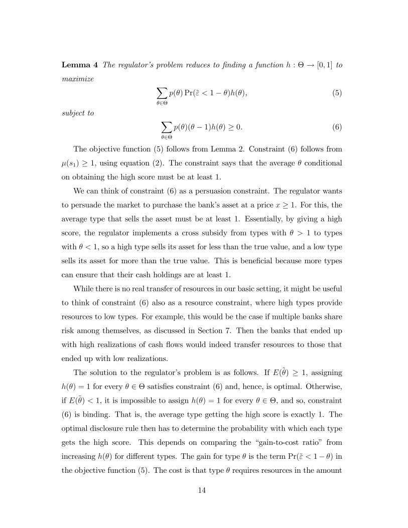
Lemma 4 The regulator’s problem reduces to finding a function h : Θ → [0, 1] to

maximize ∑θ∈Θ

p(θ) Pr(ε < 1− θ)h(θ), (5)

subject to ∑θ∈Θ

p(θ)(θ − 1)h(θ) ≥ 0. (6)

The objective function (5) follows from Lemma 2. Constraint (6) follows from

µ(s1) ≥ 1, using equation (2). The constraint says that the average θ conditional

on obtaining the high score must be at least 1.

We can think of constraint (6) as a persuasion constraint. The regulator wants

to persuade the market to purchase the bank’s asset at a price x ≥ 1. For this, the

average type that sells the asset must be at least 1. Essentially, by giving a high

score, the regulator implements a cross subsidy from types with θ > 1 to types

with θ < 1, so a high type sells its asset for less than the true value, and a low type

sells its asset for more than the true value. This is beneficial because more types

can ensure that their cash holdings are at least 1.

While there is no real transfer of resources in our basic setting, it might be useful

to think of constraint (6) also as a resource constraint, where high types provide

resources to low types. For example, this would be the case if multiple banks share

risk among themselves, as discussed in Section 7. Then the banks that ended up

with high realizations of cash flows would indeed transfer resources to those that

ended up with low realizations.

The solution to the regulator’s problem is as follows. If E(θ) ≥ 1, assigning

h(θ) = 1 for every θ ∈ Θ satisfies constraint (6) and, hence, is optimal. Otherwise,

if E(θ) < 1, it is impossible to assign h(θ) = 1 for every θ ∈ Θ, and so, constraint

(6) is binding. That is, the average type getting the high score is exactly 1. The

optimal disclosure rule then has to determine the probability with which each type

gets the high score. This depends on comparing the “gain-to-cost ratio” from

increasing h(θ) for different types. The gain for type θ is the term Pr(ε < 1− θ) inthe objective function (5). The cost is that type θ requires resources in the amount

14

1 − θ, as in equation (6). For a type θ ≥ 1, the cost is negative (or zero). Hence,

it is optimal to assign h(θ) = 1 for every θ ≥ 1. In contrast, for a type θ < 1, the

cost is positive. In this case, the gain-to-cost ratio from increasing h(θ) is

G(θ) ≡ Pr(ε < 1− θ)1− θ . (7)

It then follows from the linearity of the problem that, for types below 1, it is

optimal to set a cutoff G∗ such that types with a gain-to-cost ratio above the

cutoff are assigned h(θ) = 1, and types with a gain-to-cost ratio below the cutoff

are assigned h(θ) = 0. The optimal G∗ is the lowest cutoff possible that satisfies

constraint (6). For types with a gain-to-cost ratio that equals G∗, the probability

of obtaining the high score could be between 0 and 1 and is set such that constraint

(6) is satisfied with equality.

The following proposition summarizes the optimal disclosure rule.

Proposition 1 When the bank does not observe its type, the optimal disclosure

rule is such that

1. If E(θ) ≥ 1, then h(θ) = 1 for every θ ∈ Θ.

2. If E(θ) < 1, then

h(θ) =

{1 if θ ≥ 1 or if θ < 1 and G(θ) > G∗

0 if θ < 1 and G(θ) < G∗,(8)

where G∗ is the lowest G ∈ {G(θ)}θ<1 that satisfies∑

θ≥1 p(θ)(θ−1)+∑

θ<1:G(θ)>G p(θ)(θ−1) ≥ 0, if such G exists; otherwise, G∗ ≡ maxθ<1G(θ). If G(θ) = G∗, then

h(θ) ∈ [0, 1), such that (6) is satisfied with equality.

An interesting question is whether and when full disclosure is optimal, and

whether and when no disclosure is optimal. If E(θ) ≥ 1, we know from Proposition

1 that every type must sell its asset with probability 1. The regulator can implement

this outcome by giving all types the same score, i.e., with no disclosure. There are

other ways to implement the optimal outcome, assigning more than one score such

that the average θ of types receiving each score is at least 1. In the special case

θmin ≥ 1, the regulator can even assign a different score to each type, i.e., provide

15

full disclosure.14 In contrast, if E(θ) < 1, the regulator must assign at least two

scores. Some disclosure is necessary because, without disclosure, the price would

be less than 1 and no type would sell its asset. Yet, full disclosure is suboptimal

because under full disclosure, only types above 1 sell their assets, while under the

optimal disclosure rule, some types that are below 1 also sell their assets. Hence,

partial disclosure that pools together types above 1 with some types below 1 is the

only way to achieve the optimal outcome. The following corollary summarizes the

results above.

Corollary 1 When the bank does not observe its type, full disclosure achieves the

optimal outcome if, and only if, θmin ≥ 1. No disclosure achieves the optimal

outcome if, and only if, E(θ) ≥ 1. If E(θ) < 1, then partial disclosure is the only

way to achieve the optimal outcome.

Another interesting question is under what conditions a simple cutoff rule with

respect to θ is optimal. Interestingly, in the case of E(θ) < 1 (summarized in the

second part of Proposition 1), the types that obtain the low score are not necessarily

the lowest. So, a simple cutoff rule that assigns the high score to high types and the

low score to low types is not necessarily optimal. Intuitively, the gain from giving

the high score is higher for lower types because low types are more likely to end

up with low realizations of cash flow. That is, the numerator of (7) is decreasing

in θ. But the cost of giving the high score to low types is also higher because low

types require more resources. That is, the denominator of (7) is also decreasing in

θ. Hence, it is unclear whether G(θ) is increasing or decreasing, or whether it is

even monotone. The function G(θ), and hence the optimal disclosure rule, depends

on the distribution of the idiosyncratic risk ε.

The optimal rule will involve a simple cutoff with respect to θ when G(θ) is

increasing when θ < 1.15 In this case, types above the cutoff obtain the high score

14In fact, any disclosure rule is optimal in this special case; but see also Corollary 6.15This condition implies that the regulator’s virtual utility from assigning score s to type θ

is a quasi-supermodular function, a condition that Mensch (2018) identifies as suffi cient for amonotone disclosure rule to be optimal in a general Bayesian persuasion environment. In our

16

with probability 1, and types below the cutoff obtain the low score with probability

1. A simple example in which this happens is when there is no idiosyncratic risk

(i.e., ε = 0). Then, the gain-to-cost ratio is simply G(θ) = 11−θ . More generally, a

suffi cient condition for obtaining a cutoff rule is that the cumulative distribution

function of ε satisfies Condition 1 below. This condition is satisfied by any cumula-

tive distribution function that is concave on the positive region. Examples include

a normal distribution and a uniform distribution (both with mean zero).

Condition 1 F (ε)/ε is decreasing when ε > 0.

Corollary 2 If E(θ) < 1 and Condition 1 holds, the optimal disclosure rule in-

volves a cutoff, such that types below the cutoff obtain the low score and types above

the cutoff obtain the high score.

Another case in which the optimal rule involves a simple cutoff with respect to

θ is when r in the payoff function (1) depends on θ, according to some function r(θ)

that is increasing in θ suffi ciently strongly. This has a simple and intuitive economic

interpretation: good banks have better investment opportunities in addition to

having better assets in place. In this case, the gain from giving the high score is

r(θ) Pr(ε < 1− θ) and the gain-to-cost ratio is r(θ)G(θ). So, no matter what shape

G(θ) has, if r(θ) is increasing suffi ciently strongly, the gain-to-cost ratio will be

monotonically increasing, and the disclosure rule will look like a cutoff rule. For

example, if r(θ) = 1Pr(ε<1−θ) , then r(θ)G(θ) = 1

1−θ , which is increasing in θ.

A cutoff rule will also be optimal in a variation of our model in which the bank

can obtain the extra return r only if it sells its asset.16 For example, the bank’s

investment opportunity may expire before the asset cash flows are obtained. In

this case, the social gain from giving a high score is r, independent of type, and

the resulting gain-to-cost ratio ( r1−θ ) is increasing in type.

setting, the virtual utility from assigning the low score is 0, and the virtual utility from assigningthe high score is Pr(ε < 1− θ)− λ(1− θ), where λ > 0 is the Lagrange multiplier for constraint(6). Under the optimal disclosure rule, λ = G∗.16That is, the bank’s payoff is E(θ + ε) = E(θ), if it keeps the asset, and R(x), if it sells the

asset.

17

Finally, an example in which the optimal disclosure rule does not involve a

simple cutoff, as in Corollary 2, is when G(θ) is decreasing when θ ≤ θk+1. In this

case, the optimal disclosure rule is nonmonotone in type. It includes a cutoff such

that types below the cutoff and types above 1 obtain the high score, while types in

the middle obtain the low score. A suffi cient condition for this to happen is that

F (ε)/ε is increasing when ε ≥ 1− θk+1.17

5 Bank observes its type

So far, we assumed that the bank does not observe its type. We showed that it

is possible to implement the optimal disclosure rule with two scores, such that the

regulator pools all the types that sell under the same score. In this section, we show

that this conclusion may no longer be true when the bank observes its type. The

difference is that now each type has a “reservation price,”i.e., a minimum price at

which it is willing to sell. When different types have different reservation prices,

the regulator may need to assign more than two scores to distinguish among them.

We also discuss how the regulator should assign these multiple scores to low types

that are pooled with high types.

5.1 Derivation of the regulator’s problem

We first derive the reservation price for each type. Define

ρ(θ) =

{max{1, θ − rPr(ε < 1− θ)} if θ ≥ 1min{1, θ + rPr(ε ≥ 1− θ)} if θ < 1.

(9)

Lemma 5 In equilibrium, a bank of type θ agrees to sell at price x if and only if

x ≥ ρ(θ).

17An example of a probability distribution function that satisfies the condition above is atruncated Cauchy distribution (Nadarajah and Kotz, 2006) on the interval [−A, 0] minus itsmean, where the lower bound A depends on the model parameters. Intuitively, for the suffi cientcondition above to hold, we must have F (1− θk+1) <

1−θk+11−θmin F (1− θmin) <

1−θk+11−θmin . So, if θk+1 is

close to 1, then F (1−θk+1) ' 0, and the probability distribution of ε puts a low mass on negativevalues (and a high mass on positive values). To also satisfy E(ε) = 0, the distribution must havea fat left tail.

18

Lemma 5 is derived as follows. If type θ keeps its asset, its expected payoff is

E[R(θ + ε)] = θ + rPr(ε ≥ 1− θ). If type θ sells at price x, its payoff is R(x); i.e.,

it is x when x < 1 and x+ r when x ≥ 1. Hence, type θ agrees to sell if, and only

if, R(x) ≥ θ+ rPr(ε ≥ 1− θ). In the proof, we show that this reduces to x ≥ ρ(θ).

We refer to ρ(θ) as type θ’s reservation price and denote ρi = ρ(θi). In the

special case in which there is no idiosyncratic risk (ε = 0), the reservation price is

ρ(θ) = θ for every θ ∈ Θ, and the regulator cannot implement cross-subsidies from

high types to low types. In this case, every type θ ∈ Θ ends up with a payoffR(θ)

independently of the disclosure rule, and so, every disclosure rule is optimal.

The rest of our paper focuses on the more interesting case in which ε has a

nondegenerate distribution. In this case, the reservation price satisfies three prop-

erties, which we use later (see Figure 1). First, ρ(θ) is increasing in θ. Second,

ρ(θ) < θ when θ > 1. Third, ρ(θ) > θ when θ < 1. Intuitively, types above 1 are

willing to sell below their true valuations to guarantee that their cash holdings do

not fall below 1. This is the insurance motive. In contrast, types below 1 will agree

to sell only above their true valuation, because if they sell for the true valuation,

they lose the option value of ending up with cash holdings above 1.

Type

45­degree line

10

1

Reservation price

Figure 1.

The next lemma simplifies the analysis.

Lemma 6 Under an optimal disclosure rule:

19

1. Every type θi ≥ 1 sells its asset with probability 1.

2. If the highest type that obtains score s is θi ≥ 1, then every type sells its

asset upon obtaining that score and the price satisfies x(s) = µ(s) ≥ ρi.

3. If the highest type that obtains score s is below 1, then every type keeps its

asset upon obtaining that score.

The first part in Lemma 6 follows because if a type θ ≥ 1 did not sell its asset,

the regulator could strictly increase type θ’s payoff, without affecting the payoffs

of other types, by fully revealing θ’s type. Then, the market would offer to buy

type θ’s asset at price θ, and type θ would accept the offer. Moreover, the price

that the market would offer for the group of types that included θ initially would

remain unchanged, because it is based on the average type that sells.

The second part follows from the first part and the observation that the reserva-

tion price is increasing in θ. In particular, if the highest type that obtains score s is

θi ≥ 1, we must have x(s) ≥ ρi, so that type θi agrees to sell; and because the reser-

vation price is increasing in θ, lower types also sell upon obtaining score s. Hence,

the market prices the asset at the expected value given the score: x(s) = µ(s).

The third part reflects the fact that, if no type above 1 obtains score s, the price

x(s) must be less than 1. But then the bank will sell only if the price is strictly

above the true value, which cannot be an equilibrium outcome because the market

will overpay in expectation.

Lemma 6 implies that for each score that induces selling, the highest type that

obtains the score must be at least 1. Moreover, the sale price must be at least as

high as the reservation price of that type.

Since there are k types above 1, we can focus, without loss of generality, on

disclosure rules that assign, at most, k + 1 scores. One score, which we denote by

s0, is reserved for the types that do not sell their asset. The other k scores, which

we denote by s1, ...sk, are reserved for the types that sell their asset, such that the

highest type that obtains score si is θi.18

18Note that in Section 4, when a bank does not know its type, everyone is willing to sell for thesame price, and so, there are only 2 scores.

20

Formally, denote Si = {s ∈ S : g(s|θi) > 0 and g(s|θ) = 0 for every θ > θi}.That is, Si is the set of scores, such that the highest type that obtains each score

in Si is θi. Then:

Lemma 7 If (S, g) is an optimal disclosure rule, then (S, g), defined by S =

{s0, s1, ..., sk}, g(si|θ) =∑

s∈Si g(s|θ) for i ∈ {1, ..., k}, and g(s0|θ) = 1−∑k

i=1 g(si|θ),is also optimal.

For i ∈ {1, ..., k}, denote the probability that type θ obtains score si by hi(θ).We can write down the regulator’s problem as follows:

Proposition 2 When the bank observes its type, the regulator’s problem reduces

to choosing a set of functions {hi : Θ −→ [0, 1]}i=1,...,k to maximize

∑θ∈Θ

p(θ) Pr(ε < 1− θ)k∑i=1

hi(θ), (10)

such that (11) —(13) hold:∑θ∈Θ

p(θ)(θ − ρi)hi(θ) ≥ 0 for every i ∈ {1, ..., k}, (11)

k∑i=1

hi(θ) ≤ 1 for every θ ∈ Θ, (12)

hi(θ) = 0 for every i ∈ {1, ..., k} and θ > θi. (13)

The regulator chooses the probability hi(θ) for every θ ∈ Θ and i ∈ {1, ..., k}.The objective function (10) is as in Lemma 4, noting that the probability that type

θ sells its asset is∑k

i=1 hi(θ), rather than h(θ). Equation (11) is a generalization of

constraint (6). Now there is a constraint for every score that induces selling. The

constraint for score si (namely, constraint i) says that the average θ conditional on

obtaining score si must be at least ρi. This constraint follows since µ(si) ≥ ρi (and

(2)). Equation (12) simply says that the probability that type θ sells its asset is at

most 1. Equation (13) says that the highest type that obtains score si is type θi.

21

The problem in Proposition 2 is a linear programming problem. Because the

feasible region is bounded and closed (hi(θ) ∈ [0, 1]) and is nonempty,19 a solution

exists.

5.2 Full disclosure vs. non disclosure

As in Corollary 1, full disclosure achieves an optimal outcome if, and only if, there

are no types below 1. No disclosure achieves an optimal outcome if, and only if,

E(θ) is suffi ciently high. However, the condition for no disclosure to be optimal is

stricter than in Corollary 1, reflecting the reservation price of the highest type.

Corollary 3 When the bank observes its type, no disclosure achieves the optimal

outcome if, and only if, E(θ) ≥ ρ1. Full disclosure achieves the optimal outcome

if, and only if, θmin ≥ 1.

Note that when r is higher, the reservation price ρ1 is lower, and it is easier to

satisfy the condition for no disclosure in Corollary 3. When r is suffi ciently high,

we obtain ρ1 = 1, and the condition for no disclosure is the same as in Corollary 1.

5.3 Properties of optimal disclosure rules

The rest of this section focuses on the case E(θ) < ρ1, in which some disclosure is

necessary to achieve an optimal outcome. As we illustrate below, the solution to

the regulator’s problem continues to depend on a gain-to-cost ratio, but now there

is a different gain-to-cost ratio for every score.

Specifically, for i ∈ {1, ..., k}, the gain from assigning score si to type θ is the

term Pr(ε < 1− θ) in the objective function (10). The cost is ρi− θ, which followsfrom constraint i in (11). Hence, the gain-to-cost ratio from assigning score si to

type θ 6= ρi is

Gi(θ) ≡Pr(ε < 1− θ)

ρi − θ. (14)

While the gain does not depend on the specific score and is exactly the same as in

Section 4, the cost is different. It is more costly to assign scores that correspond19Setting hi(θ) = 1 if θ = θi, and hi(θ) = 0 if θ 6= θi, satisfies all the constraints.

22

to higher reservation prices. For types below ρi, the cost is positive, as these types

require resources when they obtain score si (they reduce the group average). For

types above ρi, the cost is negative, as these types provide resources (they increase

the group average). For use below, we refer to a score that is associated with a

higher reservation price as being higher. So score s1 is the highest, score s2 is the

second highest, and so on.

A simple case is when there is only one type above 1. Then, there is only one

score that induces selling, and the solution is similar to that in the second part of

Proposition 1, except that the gain-to-cost ratio is G1(θ) instead of G(θ). However,

if there are two or more scores that induce selling, the solution is more complicated.

Now the regulator needs to decide not only the probability that each type sells its

asset but also the allocation of the k scores that induce selling to the types that

sell.

The next proposition simplifies the analysis. It shows that there is a solution

that satisfies the following two properties. First, each type above 1 obtains the

score that is associated with its reservation price. That is, type θi > 1 obtains

score si with probability 1. Second, and perhaps counterintuitive, among the types

below 1 that sell their assets, lower types obtain higher scores.

Proposition 3 The regulator’s problem in Proposition 2 has a solution that satis-

fies the following properties:

1. hi(θi) = 1, for every i ∈ {1, ..., k}.2. hi(θv)hj(θw) = 0, for every v, ω, i, j, such that θv < θw < 1 < θi < θj. That

is, if the lower type θv obtains the lower score si, then the higher type θw does not

obtain the higher score sj.

To prove Proposition 3, we show that, if a solution does not satisfy a property,

we can construct an alternate solution that satisfies the property. The alternate

solution “saves on resources”in the sense that it weakly relaxes the constraints in

(11). Moreover, if the types above 1 have different reservation prices (ρ1 > ρ2 >

23

... > ρk), the alternate solution strictly relaxes at least one of the constraints.20

The first part in Proposition 3 reflects the fact that it is more costly to give

higher scores. Accordingly, the regulator gives each type above 1 the lowest possible

score under which the type will agree to sell. This increases the amount of resources

that types above 1 provide to cross subsidize lower types, and it also reduces the

amount of resources that the types below 1 that are matched with types above 1

end up with.

The second part in Proposition 3 reflects the fact that for the types below 1, the

relative cost of giving a higher score rather than a lower score is increasing in type.

That is, if ρj > ρi, the ratioρj−θρi−θ

is increasing in θ. The idea behind the proof is as

follows. Suppose there is a solution in which a lower type (θv < 1) obtains a lower

score (si), and a higher type (θw < 1) obtains a higher score (sj). We can save

on resources, without affecting the value of the objective function, by making the

following two changes. First, reduce the probability that the higher type obtains

the higher score and increase the probability that the lower type obtains that score.

We can choose these probabilities, such that the resource constraint for the higher

score (and hence the price for that score) is unaffected. Second, to ensure that the

probabilities that the two types sell their assets remain unchanged, increase the

probability that the higher type obtains the lower score and reduce the probability

that the lower type obtains that score. Since the relative cost of giving the higher

score rather than the lower score is increasing in type, this second change will relax

the constraint for the lower score.

Another way to see the intuition for the result above is by separating the cost

ρi− θ into two components: ρi− 1 and 1− θ. The latter is the cost of bringing thebank up to the threshold of 1, and the former is the cost of bringing it up further

from 1 to the reservation price ρi, which is associated with the score. For the types

that are slightly below 1, the second component is relatively negligible, while the

20The only case in which two types above 1 have the same reservation price is when they bothhave a reservation price of 1 (i.e., r is suffi ciently high). In this case, we can assume, withoutloss of generality, that only one score corresponds to that reservation price and that both typesobtain that score with probability 1.

24

first component is relatively first order. In contrast, for the very low types, the

second component is relatively first order. Hence, to save on resources, it is more

beneficial to reduce the first component for the types that are closer to 1. This

can be done by giving these types scores that are associated with lower reservation

prices.

In the remainder of this subsection, we focus on two subcases: E(θ) < 1 and

E(θ) ∈ [1, ρ1).

If E(θ) < 1, it is impossible to implement an outcome in which every type sells

with probability 1, and so, all the constraints in (11) are satisfied with equalities.

The intuition is similar to that in Section 4, except that now it is even harder to

implement the desired outcome in which every type sells with probability 1 because

types with reservation prices above 1 will not agree to sell for a price of 1. Formally:

Lemma 8 If E(θ) < 1, every solution to the regulator’s problem satisfies the fol-

lowing:

1. There exists a type θ < 1 for which∑k

i=1 hi(θ) < 1.

2. All the constraints in (11) are satisfied with equalities.

An immediate implication of Lemma 8 is that, for every score that induces

selling, the sale price equals to the reservation price of the highest type that obtains

the score. That is, for every i ∈ {1, ..., k}, x(si) = ρi. Another implication is

that, if the types above 1 have different reservation prices, then any solution to

the regulator’s problem must satisfy the two properties in Proposition 3. If this

were not the case, we could construct an alternate solution that strictly relaxes

one of the constraints in (11), which would violate the second part in Lemma 8.

More generally, we can show that, if there are two types above 1 with different

reservation prices, then these two types cannot obtain the same score. Combining

the implications above, we obtain the following:

Corollary 4 If E(θ) < 1, then under an optimal disclosure rule:

1. Every type above 1 sells for its reservation price.

25

2. Among the types above 1, higher types sell for (weakly) higher prices.

3. Among the types below 1 that sell with a positive probability, lower types sell

for (weakly) higher prices.

Corollary 4 implies that, unless ρ1 = ρ2 = ... = ρk, the sale price is non-

monotone in type. Among the types below 1 that sell their assets, lower types

sell for higher prices. However, among the types above 1, the opposite is true, as

these types end up selling exactly for their reservation price, which is increasing in

type. An immediate implication of Corollary 4 is that when types above 1 have

different reservation prices, the regulator must assign more than two scores that

induce selling, so that each type above 1 sells exactly for its reservation price.

Corollary 5 If E(θ) < 1 and ρ1 > ρ2 > ... > ρk, the regulator must assign at least

k + 1 scores.

Finally, if E(θ) ∈ [1, ρ1), then for some parameter values, it is possible to

implement an outcome in which every type sells with probability 1, but for some

parameter values, it is impossible to implement such an outcome. Proposition 3

suggests a simple algorithm to check whether it is possible to implement an outcome

in which every type sells with probability 1. Assign score s1 to the highest type

and to the lowest types below 1. Assign this score to as many types below 1 as

possible subject to the constraint that the average type receiving the score is ρ1

(i.e., the constraint for score s1 in (11)). Next, assign score s2 to type θ2 and

to as many of the remaining lowest types below 1, subject to constraint for score

s2; and so on.21 If the process ends when all types below 1 are assigned scores

with probability 1, then it is possible to achieve such an outcome. Otherwise, it is

impossible to implement such an outcome, and the implications are the same as in

the case E(θ) < 1.

21Equivalently, we can start pooling the lowest type above 1 (type θk) with the highest typesbelow 1 until the average θ for the group equals ρk; then pool the second lowest type above 1(type θk−1) with the remaining highest types below 1 until the average θ for the group equalsρk−1; and so on.

26

5.4 Closed-form solutions and examples

Propositions 2 and 3 provide general properties of optimal disclosure rules, along

with a general algorithm (linear programming) that can be used to determine an

optimal disclosure rule for every set of parameters and distribution functions cov-

ered by our model. To get a better idea of how optimal disclosure rules work, we

illustrate optimal disclosure rules in some special cases.

Case 1. ρ1 = 1: Here, the highest reservation price is 1. As we know from (9),

this can be consistent with having multiple types above 1, but either r is suffi ciently

high or θmax is suffi ciently low, so they are willing to sell the asset at a price of 1.

In this case, the optimal disclosure rule is identical to the one when the bank does

not observe its type, as in Proposition 1. In particular, if h(θ) solves the regulator’s

problem in Lemma 4, then h1(θ) = h(θ) and hi(θ) = 0 for every i > 1 solves the

regulator’s problem in Proposition 2; and vice versa: if {hi(θ)} solves the problemin Proposition 2, then h(θ) =

∑ki=1 hi(θ) solves the problem in Lemma 4.

Case 2. k = 1: Here, there is only one type above 1. In this case, the optimal

disclosure rule is similar to that in Proposition 1, except the gain-to-cost ratio is

G1(θ) instead ofG(θ). Corollary 2, which provides a suffi cient condition for a simple

cutoffrule to be optimal, then holds only if ρ1 is suffi ciently small. Otherwise, G1(θ)

is decreasing when θ < 1, even if Condition 1 is satisfied, and so, a simple cutoff

rule is not optimal.22 Intuitively, when ρ1 is very high, the cost ρ1− θ of giving thehigh score to type θ < 1 is very high, no matter how high θ is, and so, the dominant

factor in deciding which types should be included in risk sharing is that the gain

Pr(ε < 1− θ) is decreasing in θ. So, when ρ1 is suffi ciently high, the low types and

the only type above 1 obtain the high score, while the types in the middle obtain

the low score.

Case 3. k ≥ 2 and Gi(θ) is increasing in θ for every θ < 1 and every

i ∈ {1, ..., k}:23 Using similar logic as in Section 4, one can show that the low-

22Formally, G1(θ) is increasing when θ < 1 if, and only if, −F ′(1− θ)(ρ1 − θ) + F (1− θ) ≥ 0.This reduces to ρ

1≤ max{θ∈Θ:θ<1}{θ + F (1−θ)

F ′(1−θ)}.23A suffi cient condition for this to happen is that ρ1 < max{θ∈Θ:θ<1}{θ + F (1−θ)

F ′(1−θ)}.

27

est types are excluded from risk sharing. The optimal disclosure rule can be found

by applying the two properties in Proposition 3. First, pool the lowest type above

1 (type θk) with the highest types below 1 until all the resources from type θk are

exhausted (that is, until the average θ for the group equals ρk). Next, pool the

second lowest type above 1 (type θk−1) with the remaining highest types below 1

until the resources from type θk−1 are exhausted. And so on, until we exhaust the

resources from the highest type θ1. The following example illustrates the solution:

Example 1 There are five types θ1 > θ2 > 1 > θ3 > θ4 > θ5, and ρ1 > ρ2. So,

without loss of generality, there are three scores: s0, s1, and s2. Suppose Gi(θ) is

increasing in θ for every θ < 1 and i ∈ {1, 2}. Suppose in addition that:

p(θ2)(θ2 − ρ2) = p(θ3)(ρ2 − θ3) (15)

p(θ1)(θ1 − ρ1) = p(θ4)(ρ1 − θ4). (16)

Then, the optimal disclosure rule is as follows (an element in the table is the

probability that type θj obtains score si):

θ5 θ4 θ3 θ2 θ1

score s1 (sell at price ρ1) 1 1score s2 (sell at price ρ2) 1 1score s0 (keep asset) 1

In particular, equation (15) implies that θ3 gets score s2 with probability 1, and

equation (16) implies that θ4 gets score s1 with probability 1, so that the two

constraints in (11) are satisfied with equality. As we can see, θ1 and θ4 are pooled

together at the highest price, θ2 and θ3 are pooled together at the lower price, and

θ5 does not sell and does not participate in risk sharing.24

Case 4. k ≥ 2 and Gi(θ) is decreasing in θ for every θ < 1 and every i ∈{1, ..., k}:25 In this case, the types in the “middle”are excluded from risk sharing,

24In general, a type below 1 could be pooled with more than one type above 1. For example, ifwe changed equations (15) and (16) so that p(θ2)(θ2−ρ2) =

13p(θ3)(ρ2− θ3) and p(θ1)(θ1−ρ1) =

23p(θ3)(ρ1 − θ3) +

45p(θ4)(ρ1 − θ4), then θ3 will obtain score s1 with probability 2

3 and score s2

with probability 13 , and θ4 will obtain s1 with probability 4

5 (and s0 with probability 15 ).

25A suffi cient condition for this to happen is that ρk > max{θ∈Θ:θ<1}{θ + F (1−θ)F ′(1−θ)}.

28

and the optimal disclosure rule can be found as follows: Pool the highest type θ1

with the lowest types until all the resources from type θ1 are exhausted. Next, pool

the second highest type θ2 with the remaining lowest types, and so on, until all the

resources of the types above 1 are exhausted.

Case 5. k ≥ 2 and there exists k ∈ {1, ..., k}, such that, for every θ < 1, Gi(θ)

is decreasing in θ if i ∈ {1, ..., k} and increasing in θ if i ∈ {k + 1, ..., k}:26 In thiscase, the optimal disclosure rule can be found by combining the procedures in cases

3 and 4. The following example illustrates this.

Example 2 Suppose θ1 > θ2 > 1 > θ3 > θ4 > θ5 and ρ1 > ρ2, as in Example

1. Suppose G2(θ) is increasing when θ < 1, but G1(θ) is decreasing. Suppose

that equation (15) holds, but, instead of equation (16), we have p(θ1)(θ1 − ρ1) =

p(θ5)(ρ1 − θ5). Then, the optimal disclosure rule is as follows:

θ5 θ4 θ3 θ2 θ1

score s1 (sell at price ρ1) 1 1score s2 (sell at price ρ2) 1 1score s0 (keep asset) 1

5.5 Discussion of nonmonotonicity

Optimal disclosure rules may exhibit two forms of nonmonotonicity. First, the

probability of selling the asset may be nonmonotone in type (Example 2 and the

discussion at the end of Section 4). Second, for the types that sell, the sale price

may be nonmonotone in type (Corollary 4 and Examples 1 and 2).

The first form of nonmonotonicity arises when the gain-to-cost ratio is decreas-

ing in θ. A necessary condition for this is that the gain, which follows from the

coeffi cient of∑n

i=1 hi(θ) in the regulator’s objective function is decreasing in θ when

θ < 1. In other words, the regulator has a preference for helping lower types. In

our model, this happens because, without engaging in risk sharing, lower types are

more likely to end up with cash holdings below 1.

26A suffi cient condition for this to happen is that ρk > max{θ∈Θ:θ<1}{θ + F (1−θ)F ′(1−θ)} > ρk+1.

29

The second form of nonmonotonicity follows from the tension between the reg-

ulator’s desire to pool different types together and the types’participation con-

straints. For this tension, it is important that there is some social benefit from

insurance across different types and that the bank has some private information

related to the information that the regulator has. However, the specific form of

insurance is not crucial. For example, nonmonotonicity will continue to hold if we

replace the coeffi cient Pr(ε < 1− θ) in the regulator’s objective function with someother positive coeffi cient that depends on θ. Nonmonotonicity will also prevail if

we alter our model so that the bank must sell its asset at price x ≥ 1 to obtain r

(footnote 16). In this case, the idiosyncratic risk ε does not affect the bank’s payoff

function, yet pooling types together continues to be socially desirable to ensure

that the price is at least 1.27 If, however, the bank could obtain r by selling at any

price, full disclosure would clearly be optimal, as there would be no social surplus

from insurance; this case boils down to a simple setting of gains from trade with

adverse selection.

Another case in which nonmonotonicity will prevail is if the bank is risk averse,

namely the bank’s payoff is given by some concave function rather than the dis-

continuous function in (1).28 In this case, the optimal disclosure rule can be found

using a similar algorithm as in case 4 in Section 5.4, but with the following ad-

justment. As long as there remain types that have not been assigned a score, we

will continue to match the highest type of the remaining types with the lowest

remaining types. So in contrast to Lemma 6, every type will end up selling its

asset.29

27In this case, type θ’s reservation price is ρ(θ) = θ, if θ < 1, and ρ(θ) = max{1, θ−r}, if θ ≥ 1,which does not satisfy the third property of the reservation price in Section 5.1. Hence, the thirdpart in Lemma 6 will not necessarily hold. In particular, for any disclosure rule in which a typebelow 1 keeps its asset, there will be a payoff equivalent rule in which that type sells its asset forthe true value. The wording in Proposition 4 and the third part of Corollary 4 will need to beadjusted to reflect that.28For more details, see the last paragraph in the proof of Lemma A-1 in the appendix.29For a complete analysis of our model with a concave payoff function, see a follow-up paper

by Garcia, Teper, and Tsur (2017).

30

6 Bank can affect the value of its asset

A natural question is whether we should expect to see nonmonotone rules in prac-

tice. Alternatively, one could ask whether nonmonotone rules will continue to

prevail if we enrich our model. In this section, we show that once we add two

additional assumptions to our model, optimal disclosure rules become monotone.

The first assumption is that the bank can affect the value of its assets. Specifi-

cally, we assume that before the regulator learns the value of θ, the bank can reduce

its θ by freely disposing its assets. This assumption leads to an additional constraint

that the bank’s expected equilibrium payoff is weakly increasing in type.30

The second assumption is that the regulator cannot randomize. That is, g(s|θ)can take only the values 0 and 1. This could be viewed as a practical constraint on

what regulators can do.

Proposition 4 below characterizes optimal disclosure under the two assumptions

above. The proposition shows that an optimal disclosure rule involves two cutoffs

zL ≤ zH . The role of zL is to determine which types sell their assets. Types below

zL sell with probability 0, while all the other types sell with probability 1. The

role of zH is to determine which types are pooled together. Types on the interval

[zL, zH ] sell for the same price, and they can all obtain the same score. Types above

zH sell at higher prices to reflect their higher reservation prices. If the average θ of

the types above zH is at least ρ1, it is possible to implement optimal disclosure by

giving all the types above zH the same score. Otherwise, it is impossible to do so,

and for some parameter values, the only way to implement optimal disclosure is by

giving each type above zH its own score.

The optimal cutoffs zL, zH can be found as follows. For a given zH , it is optimal

to set zL as low as possible, subject to the constraint that the average cash flow

for the types on [zL, zH ] is at least ρ(zH). This constraint can be satisfied only if

30Note that this constraint is violated in Examples 1 and 2. For instance, in Example 1, typeθ4’s expected equilibrium payoff is higher than type θ3’s expected equilibrium payoff.

31

zH ≥ 1, and it reduces to zL = zL(zH), where

zL(zH) = min{z ∈ Θ :∑

θ∈[z,zH ]

p(θ)[θ − ρ(zH)] ≥ 0}. (17)

The optimal zH minimizes zL(zH).

Formally, denote z∗H = arg minzH∈{Θ:θ≥1} zL(zH).31 The optimal outcome is

summarized in the next proposition.

Proposition 4 Suppose the bank can freely dispose assets and the regulator must

follow a deterministic disclosure rule. Then under an optimal disclosure rule:

1. Types below zL(z∗H) do not sell their assets, types that belong to the interval

[zL(z∗H), z∗H ] sell at the same price, and types above z∗H sell at a higher price (or

prices).

2. If zL(θ) = θ for every θ > z∗H , then every type above z∗H must obtain a

different score and sell at a different price.

Intuitively, the choice of zH involves a tradeoff. A higher zH increases the

resources that are available to cross subsidize types below 1, but it also requires an

increase in the resources that each type on [zL(zH), zH ] should end up with, because

these required resources are determined by the reservation price of zH . The optimal

zH balances these two forces.32

In general, an optimal disclosure rule must include at least three scores to

distinguish among the types that do not sell, the types that sell at the same price,

and the types that sell at a higher price (or prices). In some cases, more than three

scores are needed to distinguish among the high types that sell.

Interestingly, for some parameter values, an optimal disclosure rule must assign

each type a different score, i.e., provide full disclosure.33 Formally, recall that the

lowest type is θmin = θm and the second lowest type is θm−1. Then:

31If the set argminz2∈Θ z1(z2) contains more than one number, then any of them is optimaland any of them satisfies Proposition 4.32Example 3 in the appendix illustrates this tradeoff.33This last result holds even if the bank cannot freely dispose asset, but under a smaller set of

parameters. (The proof contains more details.)

32

Corollary 6 Suppose the bank can freely dispose assets and the regulator must

follow a deterministic disclosure rule. Then, if θm−1 ≥ 1 and zL(θ) = θ for every

θ ≥ θm−1, the only way to implement an optimal outcome is by full disclosure.

Corollary 6 illustrates two cases in which full disclosure is necessary. In the first

case, all types are above 1 (θm ≥ θm−1 ≥ 1) but have very different reservation

prices. Full disclosure is necessary because no type is willing to sell at a price that

reflects the average of a group that includes that type and lower types. The second

case is similar to the first case, but there is an additional type below 1 (θm < 1),

which ends up keeping its asset.34

Finally, one could ask what happens if banks can freely dispose assets and the

regulator can randomize. In an earlier draft, we analyze this case. We show that,

perhaps surprisingly, for some parameter values, the two forms of nonmonotonicity

in Section 5.5 continue to hold. In particular, for some parameter values, lower

types continue to sell at higher prices. However, to ensure that the equilibrium

payoff is weakly increasing in type, these lower types sell with a probability that is

less than 1. We also show that, for some parameter values, some types above 1 sell

above their reservation prices. This is beneficial because it allows the lower types

that obtain high scores to sell with a higher probability, while still ensuring that

the equilibrium payoff is increasing in type.35

7 Discussion and extensions

In this section, we discuss some of the assumptions, interpretations, and possible

extensions of the model.

1. We assumed that the bank’s payoff function (1) exhibits some discontinuity.

This assumption is important for the basic tradeoff in our model when the bank

does not observe its type, because it implies that disclosure can not only reduce

risk sharing opportunities as in Hirshleifer (1971) but is also sometimes necessary

34The second case is consistent with E(θ) < 1 as well as with E(θ) ≥ 1.35Note that some types above 1 could sell above their reservation prices also in the case discussed

in Proposition 4.

33

to prevent risk sharing markets from breaking down. The latter effect is a direct

consequence of our discontinuity assumption and would not be obtained if we had

a traditional specification of insurance motive, namely a risk averse bank with a

standard concave utility function. In contrast, the discontinuity in the bank’s payoff

function is not necessary for our main results for the case in which the bank knows

its type. As we explained in Section 5.5, a concave payoff function will lead to

similar results.

2. In our model, the bank shares risk with the market. The nature of our results

remains the same if banks enter risk-sharing arrangements among themselves rather

than with the market (e.g., as in Allen and Gale, 2000; Leitner, 2005), provided

that idiosyncratic risk is fully diversified within a group. This is the case if there is

a continuum of banks of each type, or if there are two banks of each type, one with

cash flow θ + ε and one with θ − ε. This is also the case if the regulator providesinsurance against idiosyncratic risk within a group.

3. In our model, the regulator discloses information about the value of existing

assets. In practice, stress tests are designed to assess how the bank would perform

under some hypothetical stress scenario. Yet, information from stress tests can

still have a significant impact on current values. First, if the probability of the

stress scenario is suffi ciently high, stress test results will clearly affect current asset

values. Second, stress tests results will also have a significant impact on current

values if the regulator requires the bank to take some action (e.g., increase capital),

which is costly to the bank, say, by preventing the bank from implementing its

desired investment strategy. Our model suggests that, rather than provide detailed

information about how each bank would perform under stress scenarios, it might

be optimal to just say what action each bank should take. Moreover, it might be

optimal to require banks of different levels of strength to take the same action (see

more below).

4. An interesting extension of our model would allow the regulator to provide

funds to banks. Such an extension would suggest that, in some cases, it is optimal to

inject money not only to weak banks but also to strong banks so that the market

34

cannot distinguish among them.36 For example, suppose there are two banks:

strong (θ1 = 1.2, ρ1 = 1) and weak (θ2 = 0.4 ), and the regulator has a bailout

fund in the amount of 0.4. Suppose that the regulator would like each bank to end

up with at least one dollar and that both banks can raise cash by issuing equity.

Giving all the money to the weak bank identifies this bank as weak; and because

the value of the weak bank after the cash injection is 0.8, that bank will not be

able to raise one dollar by issuing equity. Splitting the money equally between the

two banks leads to a better outcome. Now, after the cash injection, the value of

the strong bank is 1.4, and the value of the weak bank is 0.6. But since the market

cannot distinguish between the two banks, each bank can sell its equity for a price

of 1, which is the average value of both banks. So, both banks can guarantee cash

holdings of 1.37

5. In our model, all the economic surplus is captured by the banking sector,

and so, the regulator sets a disclosure rule aiming to maximize the surplus in the

banking sector. Our model can easily capture externalities that banks impose on

the rest of society. For example, suppose that when a bank of type θ fails (θ+ε < 1),

society suffers some exogenous loss l(θ). Then, the social gain from having a bank

sell its asset is higher by l(θ). We can include this gain in the regulator’s objective

function and take it into account in the design of the disclosure rule.38 Our main

36Indeed, one of the first uses of the Troubled Asset Relief Program (TARP) funds was providingcapital to nine major financial institutions as part of the Capital Purchase Program, a programdesigned to infuse capital to “healthy”banks. During the audit, former Federal Reserve ChairBen Bernanke told the Special Inspector General for the TARP that “there were differences in thenine banks in terms of strength and weakness, but that the selection was generalized in order toavoid stigmatizing any one bank as being a weak bank and creating panic.”(See SIGTARP report10-001, “Emergency capital injections provided to support the viability of Bank of America, othermajor banks, and the U.S. financial system,”October 2009.)37We can extend the example to show that, in some cases, it is optimal to create two groups

of banks, each containing strong banks and weak banks, and inject cash only to banks in onegroup. For example, suppose there are four banks: θ1 = 2.2, θ2 = 1.2, θ3 = 0.4, θ4 = 0.2, withρ1 = 1.2 and ρ2 = 1. Then it is optimal to have θ2 and θ3 in one group (as before) and θ1 and θ4

in another group, and it is optimal to split the bailout money (0.4) equally only among banks inthe first group. Then every bank can raise at least $1 by selling equity. Banks θ2 and θ3 will sellfor $1, and banks θ1 and θ4 will sell for $1.2.38Specifically, we can replace the regulator’s objective function (10) with

∑θ∈Θ p(θ) Pr(ε <

1− θ)[r + l(θ)]∑ki=1 hi(θ).

35

results continue to hold in this case. Clearly, now the regulator will have a stronger

motive to help banks with a high l(θ). This may capture the familiar “too big to

fail”argument, whereby regulators try to save institutions whose failure could pose

a substantial damage to the economy.

6. As in any standard mechanism design problem, we assumed that the regu-

lator can commit to assigning scores according to the announced disclosure rule;

in particular, the regulator does not lie. In our basic setting, this assumption is

crucial because ex post the regulator could gain by giving a score that induces

selling instead of a score that does not induce selling. In some cases, the com-

mitment not to lie arises endogenously. For example, if banks share risk among

themselves, rather than with a third party, and the optimal disclosure rule has two

scores, as in Proposition 1, then the regulator cannot gain ex post by lying. If he

lies, banks will have insuffi cient funds to honor the agreements, and they could all

fail by contagion.39 However, if the ex ante optimal disclosure rule has a group

whose average θ is more than 1 (i.e., ρ1 > 1), the regulator could gain ex post

by adding more types to that group, as long as the group average is at least 1.

Anticipating that, types with reservation prices above 1 will not agree to partic-

ipate in risk sharing. To overcome this problem, the regulator could supplement

the disclosure policy with other instruments, such as guaranteeing payments under

these risk-sharing arrangements, or providing convincing evidence that the average

θ for a group receiving a given score is as high as announced.

7. Another aspect of commitment is that the regulator cannot alter the disclo-

sure rule ex post, once he learns the bank’s type. This type of commitment arises

naturally if there is a continuum of banks and the probability p(θ) of being a type θ

represents the proportion of banks of this type in the continuum. Then, maximizing

each bank’s ex-ante expected payoff is the same as maximizing the sum of banks’

ex-post payoffs. Since the regulator is interested in that, he has no incentive to

deviate to another disclosure rule ex post.40 In this sense, the regulator is different

39This would be true, even if the regulator privately observed the aggregate state.40This aspect of commitment holds, even if risk sharing is between the bank and the market,

36

from a single bank. A strong bank will have incentive to reveal itself as strong, even

when it is socially optimal that the bank is pooled together with weaker banks.

8. The discussion above suggests that studying disclosure by the regulator and

not by individual banks is very natural in the context of our model. First, ex ante,

the regulator and banks may have different objective functions because the regu-

lator cares about externalities that banks impose on the rest of society.41 Second,

ex-post, the regulator’s commitment to a disclosure rule arises more naturally than

that of an individual bank.

9. Assigning a score is equivalent to recommending a price to the market. A

high score does not necessarily mean that the bank is strong. It only means that

the average cash flow conditional on obtaining the score equals the recommended

price. One can also think of scores more broadly. Scores separate banks into

groups, and assigning scores is isomorphic to recommending to the banks which

groups to form. For example, one can think of scores as suggesting mergers among

banks; or if we applied our ideas to Leitner’s (2005) setting, scores could suggest

joint liability arrangements. Our model provides a characterization of optimal

groups that could emerge following disclosure when each bank can choose whether

to join the recommended group or stay in autarky and under the assumption that

idiosyncratic risk is fully diversified within a group. In one interpretation, our model

illustrates how the regulator’s disclosure policy affects the financial networks that

banks form.42

10. We believe that our model can be used as a benchmark to think of credit

rating agencies. Our model suggests that coarse ratings as well as low types receiv-

ing high ratings may be a feature of a socially optimal outcome. This is different

from other papers (e.g., Kartasheva and Yilmaz, 2013; Goel and Thakor, 2015), in

which coarse ratings reduce welfare. An interesting question is what the optimal

as is explicitly assumed in our basic setting.41The idea that the regulator and banks may have different incentives to disclose information

is also explored in Alvarez and Barlevy (2015).42We do abstract, however, from other issues of group formation, such as whether a bank

receiving one score will attempt to form a link with a bank receiving a different score.

37

disclosure rule looks like when the regulator faces competition from credit rating

agencies or whether it is possible to implement risk sharing when the regulator and

credit rating agencies have different objectives.

11. We could interpret our paper as one about the design of stress tests rather

than disclosure. In particular, choosing a disclosure rule is the same as designing

an experiment (e.g., stress tests) that provides a public signal s ∈ S according

to some distribution g(s|θ). With this interpretation, the regulator’s commitmentboils down to committing not to manipulate the public signal.

12. Our basic setup maps into a general Bayesian persuasion game (Kamenica

and Gentzkow, 2011) with one sender (the regulator) and one receiver (the market)

whose equilibrium action (price offered) equals the expected state (bank’s type)

conditional on posterior beliefs.43 The standard concavification approach has lim-

ited applicability in characterizing optimal disclosure rules in our setting because

if the bank observes its type, the equilibrium price generally depends on the entire

distribution of types given the market’s posterior beliefs. In particular, the equilib-

rium price x is a fixed point of E(θ|ρ(θ) ≤ x), where E denotes the expected value

given the market’s posterior beliefs, and the condition ρ(θ) ≤ x reflects the fact

that the bank agrees to sell only if the price is above its reservation price.44 If the

bank does not observe its type, the equilibrium price is simply x = E(θ), but the

standard concavification approach still has limited applicability in characterizing

optimal disclosure rules, because the regulator’s payoffdepends on the bank’s type:

it is r if x ≥ 1 and rPr(ε ≥ 1− θ) if x < 1.45

13. Our results on optimal disclosure rules could be applied to other settings

of Bayesian persuasion in which disclosure is followed by a game in which an unin-

formed receiver makes a price offer to a third party that has the information that

the sender has and that can either accept or reject the offer. For example, consider

43So, the market can be viewed as having a quadratic utility function: −(x− θ)2.44More recent approaches (e.g., Gentzkow and Kamenica, 2016; Kolotilin, forthcoming; Dwor-

czak and Martini, 2017) also have limited applicability in characterizing optimal disclosure rulesin our setting.45If the bank observes its type, the regulator’s payoff is r if x ≥ ρ(θ) and rPr(ε ≥ 1 − θ) if

x < ρ(θ).

38

schools that grade students with different abilities and potential employers who care

about the average ability of the students they hire. Suppose that students know

their own abilities and can open their own businesses instead of getting hired. In

this case, a student’s reservation price is the benefit from opening his own business.

Our analysis can shed light on the way schools will communicate information about

students.46 In different settings, reservation prices could also reflect payoffs that

informed third parties could obtain by signaling their types.

8 Conclusion

We provide a model of an optimal disclosure policy of a regulator who has informa-

tion about banks. The disclosure policy affects whether banks can take corrective

actions, particularly whether banks can engage in risk sharing to ensure that their

capital does not fall below some critical level.

We show that, if the average forecasted capital is suffi ciently high, E(θ) > ρ1,

then no disclosure is necessary. Otherwise, some disclosure is necessary, which

generally takes the form of partial disclosure, pooling together banks of different

levels of strength. If banks do not know their types, two scores are suffi cient, and,

in many cases, a simple cutoff rule is optimal. If a bank knows its type, more

scores are needed, and, in general, an optimal disclosure is nonmonotone in that

the price at which a bank can sell its asset is nonmonotone in type. However, this

nonmonotonicity disappears if banks can freely dispose assets and the regulator

must follow a deterministic disclosure rule. In this case, an optimal disclosure rule

generally involves two thresholds, such that, banks below the lower threshold are

excluded from risk sharing, those in the middle are pooled together at a price that

reflects the average capital for the group, and those above the higher threshold are

valued at higher prices that reflect their higher reservation values. In some cases,

full disclosure is necessary.

We discuss a few extensions, such as the case in which the regulator can inject

46Ostrovsky and Schwarz (2010) study a similar problem, but without such reservation prices.

39

money to banks. There are many other interesting extensions, some of which

have been explored recently. For example, Williams (2017) studies how optimal

disclosure affects a bank’s ex-ante portfolio choice; Inostroza and Pavan (2017)

study a case in which market participants have heterogeneous beliefs; and Orlov,

Zryumov, and Skrzypacz (2017) study the joint problem of optimal disclosure and

capital requirements when the banks’ portfolios are correlated. We believe the

model results could also be used to characterize optimal signals in other Bayesian

persuasion problems, outside the banking arena.

Finally, there are important issues related to disclosure in stress tests beyond the

disclosure of the test results. Leitner andWilliams (2017) study whether a regulator

should reveal its stress-testing model to banks. Leitner and Yilmaz (forthcoming)

study the extent to which a regulator should rely on bank internal risk models.

Appendix

Proof of Lemma 1. From the text, the equilibrium price is x(s) = µ(s). Con-

ditional on the bank’s information, the bank’s expected payoff is E[R(θ + ε|s =

s)] = µ(s) + rPr(θ+ ε ≥ 1|s = s) if it keeps the asset, and R(µ(s)) if it sells. From

Assumption 1, µ(s)+r > E[R(θ+ ε|s = s)] > µ(s). Hence, if µ(s) ≥ 1, it is optimal

for the bank to sell because R(µ(s)) = µ(s) + r > E[R(θ + ε|s = s)]. If µ(s) < 1,

it is optimal to keep the asset because R(µ(s)) = µ(s) < E[R(θ + ε|s = s)].

Proof of Lemma 2. The regulator chooses a disclosure rule (S, g) to maximize∑θ∈Θ p(θ)u(θ). Observe that,∑θ∈Θ

p(θ)∑

s:µ(s)≥1

µ(s)g(s|θ) =∑

s:µ(s)≥1

µ(s)∑θ∈Θ

p(θ)g(s|θ)

=∑

s:µ(s)≥1

∑θ∈Θ

θp(θ)g(s|θ) =∑θ∈Θ

p(θ)∑

s:µ(s)≥1

θg(s|θ),

(A-1)

40

where the second equality follows from equation (2). Hence,∑θ∈Θ

p(θ)u(θ) =∑θ∈Θ

p(θ)∑

s:µ(s)<1

[θ + rPr(ε ≥ 1− θ)]g(s|θ) +∑θ∈Θ

p(θ)∑

s:µ(s)≥1

[θ + r]g(s|θ)

=∑θ∈Θ

p(θ)[θ + rPr(ε ≥ 1− θ)]∑

s:µ(s)<1

g(s|θ) +∑θ∈Θ

p(θ)[θ + r]∑

s:µ(s)≥1

g(s|θ).

(A-2)

Since∑

s:µ(s)<1 g(s|θ) = 1−∑

s:µ(s)≥1 g(s|θ), we obtain that∑θ∈Θ

p(θ)u(θ) =∑θ∈Θ

p(θ)[θ+ rPr(ε ≥ 1− θ)] + r∑θ∈Θ

p(θ) Pr(ε < 1− θ)∑

s:µ(s)≥1

g(s|θ).

(A-3)

In the right-hand side of (A-3), only the second term is affected by the disclosure

rule. Hence, maximizing∑

θ∈Θ p(θ)u(θ) is the same as maximizing∑

θ∈Θ p(θ) Pr(ε <

1− θ)∑

s:µ(s)≥1 g(s|θ).

Proof of Lemma 3. For s ∈ S, denote µ(s) = E[θ|s = s], where the expecta-

tion is calculated under g.

Suppose first that∑

θ∈Θ p(θ)g(s1|θ) > 0 and∑

θ∈Θ p(θ)g(s0|θ) > 0. From (2),

the definition of g, and the law of iterated expectations,

µ(s1) =

∑θ∈Θ θp(θ)g(s1|θ)∑θ∈Θ p(θ)g(s1|θ)

=

∑θ∈Θ p(θ)

∑s:µ(s)≥1 µ(s)g(s|θ)∑

θ∈Θ p(θ)∑

s:µ(s)≥1 g(s|θ) . (A-4)

Hence, µ(s1) ≥ 1. Similarly, µ(s0) < 1. From Lemma 1, under (S, g), the bank

sells its asset with probability∑

s:µ(s)≥1 g(s|θ); and under (S, g), the bank sells with

probability g(s1|θ). From the definition of g(s1|θ), these two probabilities are thesame. Lemma 2 then implies that the value of the objective function is also the

same under both rules.

In the special case∑

θ∈Θ p(θ)g(s1|θ) = 0, we have that g(s1|θ) = 0 for every

θ ∈ Θ. Hence, under (S, g), Pr(s = s1) = 0 and Pr(s = s0) = 1; and under (S, g),

every type obtains a score with µ(·) < 1 with probability 1. Hence, from the law of

iterated expectations, under (S, g), E(θ) = µ(s1) Pr(s = s1) + µ(s0) Pr(s = s0) =

µ(s0); and under (S, g), E(θ) =∑

s∈S µ(s) Pr(s = s) < 1. Hence, µ(s0) < 1. Hence,

under both disclosure rules, the bank sells with probability 0.

41

Similarly, if∑

θ∈Θ p(θ)g(s0|θ) = 0, it follows that µ(s1) = E(θ) ≥ 1, and under

both disclosure rules, the banks sells with probability 1.

Proof of Lemma 4. As a preliminary, observe that from (2), µ(s) ≥ 1 if and

only if∑

θ∈Θ p(θ)(θ − 1)g(s|θ) ≥ 0.

From Lemma 3, we can focus, without loss of generality, on disclosure rules

(S, g) that assign at most two scores s0, s1, such that µ(s1) ≥ 1 and µ(s0) < 1.

(As in Lemma 3, µ(·) denotes the conditional expectation under g.) We first showthat, if such (S, g) solves the problem in Lemma 2, then h(θ) = g(s1|θ) solvesthe problem in Lemma 4. Specifically, since µ(s1) ≥ 1, h satisfies constraint (6).

Now suppose, to the contrary, that there exists h : Θ → [0, 1] that satisfies (6)

and gives a higher value for the objective function (5); that is,∑

θ∈Θ p(θ) Pr(ε <

1 − θ)h(θ) >∑

θ∈Θ p(θ) Pr(ε < 1 − θ)h(θ). Construct an alternate disclosure

rule (S ′, g′), defined by: S ′ = {s′0, s′1}, g′(s′1|θ) = h(θ), and g′(s′0|θ) = 1 − h(θ).

Since h satisfies (6), then under (S ′, g′) (and when µ′(·) is calculated under g′),µ′(·) ≥ 1, at least for score s′1. Hence, the value of the objective function (4) is at

least∑

θ∈Θ p(θ) Pr(ε < 1 − θ)g′(s′1|θ) =∑

θ∈Θ p(θ) Pr(ε < 1 − θ)h(θ). In contrast,

under (S, g), the value of the objective function (4) is only∑

θ∈Θ p(θ) Pr(ε < 1 −θ)g(s1|θ) =

∑θ∈Θ p(θ) Pr(ε < 1 − θ)h(θ). But this contradicts the optimality of

(S, g).

Next, we show that if h solves the problem in Lemma 4, then (S, g), defined by

S = {s0, s1}, g(s1|θ) = h(θ), and g(s0|θ) = 1 − h(θ) solves the problem in Lemma

2. Suppose, to the contrary, that there is a disclosure rule (S, g) that gives a higher

value to (4). Without loss of generality, S = {s0, s1}, and when µ(·) is calculatedunder g, µ(s1) ≥ 1 and µ(s0) < 1. Hence,

∑θ∈Θ p(θ)g(s1|θ) >

∑θ∈Θ p(θ) Pr(ε <

1− θ)g(s1|θ) >∑

θ∈Θ p(θ) Pr(ε < 1− θ)g(s1|θ) ≥ 0. Now let h(θ) = g(s1|θ). Then,h satisfies (6) and gives a higher value for (5) than h. But this contradicts the

optimality of h.

Proof of Proposition 1. By Assumption 1, the coeffi cient of h(θ) in (5) is

positive.

42

Part 1: Setting h(θ) = 1 for every θ ∈ Θ achieves the maximal attainable value

for (5) and satisfies constraint (6). Any other h : Θ → [0, 1] reduces the value of

(5).

Part 2: Clearly, h(θ) = 1 for every θ ≥ 1, because a higher h(θ) increases the

value of (5) and weakly relaxes the constraint (6). However, setting h(θ) = 1 for

every θ ∈ Θ violates (6). Hence, (6) is binding.

Next, we show that if h(θ) > 0 for some θ < 1, then h(θ) = 1 for every θ ∈ Θ,

such that G(θ) > G(θ). That is, if type θ < 1 sells its asset with some positive

probability, then every type with a higher gain-to-cost ratio sells with probability

1. Suppose, to the contrary, that a type θ′ < 1 exists, such that G(θ′) > G(θ) but

h(θ′) < 1. We obtain a contradiction to the optimality of h by constructing an

alternate solution:

h(θ) =

h(θ) if θ /∈ {θ′, θ}h(θ) + ∆ if θ = θ′

h(θ)− p(θ′)(1−θ′)p(θ)(1−θ) ∆ if θ = θ

. (A-5)

In particular, if∆ > 0 is suffi ciently small, h is a function fromΘ to [0, 1]. Moreover,

h satisfies (6) and increases the value of (5) by p(θ′) Pr(ε < 1− θ′)∆− p(θ) Pr(ε <

1− θ)p(θ′)(1−θ′)

p(θ)(1−θ) ∆, which equals ∆p(θ′)(1− θ′)[G(θ′)−G(θ)] > 0.

Hence, there exists a type θ∗ < 1, such that, for every θ < 1, h(θ) = 1 if

G(θ) > G(θ∗); and h(θ) = 0 if G(θ) < G(θ∗). Let G∗ = G(θ∗). Then to satisfy (6),

we must have∑θ≥1

p(θ)(θ − 1) +∑

θ<1:G(θ)>G∗

p(θ)(θ − 1) +∑

θ<1:G(θ)=G∗

p(θ)(θ − 1)h(θ) = 0. (A-6)

The result then follows immediately. (Note that there could be more than one type

θ < 1, such that G(θ) = G∗. In that case, there is more than one combination of

{h(θ)}θ:G(θ)=G∗ that satisfies (6).)

Proof of Corollary 1. Since θmax > 1, it follows from Proposition 1 that,

under an optimal disclosure rule, at least one type below 1 sells with a positive

probability.

43

Under full disclosure, type θ is offered price θ (i.e., type θ obtains a score s such

that µ(s) = θ). So, type θ ≥ 1 sells with probability 1, and type θ < 1 sells with

probability 0. If θmin ≥ 1, full disclosure is optimal because every type sells with

probability 1. If θmin < 1, full disclosure is suboptimal because no type below 1

sells.

Under no disclosure, µ(s) = E(θ) for every s ∈ S. If E(θ) ≥ 1, every type sells

with probability 1, which is optimal. If E(θ) < 1, every type sells with probability

0, which is suboptimal.

Finally, if E(θ) < 1, then θmin < 1. Hence, neither full disclosure nor no

disclosure is optimal. In other words, partial disclosure is the only way to achieve

the optimal outcome.

Proof of Corollary 2. Let θi < θj < 1. Then 1 − θi > 1 − θj > 0. From

condition 1, G(θi) < G(θj). The result then follows from Proposition 1.

Proof of Lemma 5. The main argument is in the text. It remains to show

that

R(x) ≥ θ + rPr(ε ≥ 1− θ) (A-7)

reduces to x ≥ ρ(θ).

Case 1: θ ≥ 1. If x ≥ 1, (A-7) is satisfied if, and only if, x + r ≥ θ + rPr(ε ≥1 − θ). If x < 1, (A-7) is violated because R(x) < 1. Hence, (A-7) is satisfied if,

and only if, x ≥ max{1, θ − rPr(ε < 1− θ)} = ρ(θ).

Case 2: θ < 1. If x ≥ 1, (A-7) is satisfied because R(x) ≥ 1 + r. If x < 1, (A-7)

is satisfied if, and only if, x ≥ θ + rPr(ε ≥ 1− θ). Hence, (A-7) is satisfied if, andonly if, x ≥ min{1, θ + rPr(ε ≥ 1− θ)} = ρ(θ).

Proof of Lemma 6. Consider an optimal disclosure rule (S, g).

Part 1: Suppose, to the contrary, that there exist a type θ′ ≥ 1 and a score

s′ ∈ S, such that g(s′|θ′) > 0, and such that θ′ does not sell upon obtaining score

44

s′. Construct an alternate rule, defined by: S = S ∪ {s},

g(s|θ′) =

g(s′|θ′) if s = s0 if s = s′

g(s|θ′) if s /∈ {s′, s},

and, for θ 6= θ′,

g(s|θ) =

{g(s|θ) if s 6= s0 if s = s.

Under (S, g), the only type that obtains score s is θ′. So, the equilibrium price for

score s is θ′. By Lemma 5, θ′ sells upon obtaining score s. Since the price of each

score reflects the average θ of all the types that sell under the score, equilibrium

prices for all other scores remain unchanged. Hence, the alternate rule increases

the expected payoff for type θ′ by rg(s′|θ′) Pr(ε < 1− θ′), while keeping the payoffsfor all other types unchanged. But this contradicts the optimality of (S, g).

Part 2: Suppose the highest type that obtains score s is θi ≥ 1. That is,

θi = max{θ ∈ Θ : g(s|θ) > 0}. From part 1, type θi sells its asset upon obtaining

score s. So, by Lemma 5, x(s) ≥ ρi. Because ρ(θ) is increasing in θ, any other

type that obtains score s also sells upon obtaining score s. Hence, selling does not

convey additional information to the market. Hence, the price is x(s) = µ(s).

Part 3: Suppose the highest type that obtains score s is θi < 1. Suppose, to the

contrary, that some types sell upon obtaining score s, and that the highest type

that sells is θ < 1. Since the market does not expect to lose money, the price must

satisfy x(s) ≤ θ. And since θ < 1, we know that θ < ρ(θ). But then x(s) < ρ(θ),

which contradicts Lemma 5.

Proof of Lemma 7. Suppose (S, g) is an optimal disclosure rule. From Lemma

6 and the definition of Si, type θ sells its asset upon obtaining score s ∈ S if, andonly if, s ∈ ∪ki=1Si. Moreover, the sale price is x(s) = µ(s). Hence, type θ’s

expected payoff is

u(θ) =∑

s/∈∪ki=1Si

[θ + rPr(ε ≥ 1− θ)]g(s|θ) +∑

s∈∪ki=1Si

[µ(s) + r]g(s|θ). (A-8)

45

Following the steps in Lemma 2, but replacing the conditions µ(s) < 1 and µ(s) ≥ 1

with s /∈ ∪ki=1Si and s ∈ ∪ki=1Si, respectively, we can show that the regulator’s payoff

reduces to

r∑θ∈Θ

p(θ) Pr(ε < 1− θ)∑

s∈∪ki=1Si

g(s|θ), (A-9)

plus a constant term that does not depend on the disclosure rule.

Now consider (S, g). It is easy to verify that (S, g) is a disclosure rule. For

every si ∈ S, such that∑

θ∈Θ p(θ)g(si|θ) > 0, denote µ(si) = E[θ|s = si], where

the expectation is calculated under g. (If∑

θ∈Θ p(θ)g(si|θ) = 0, then g(si|θ) = 0

for every θ ∈ Θ, and the set Si is empty.)

From (2), the definition of g, the law of iterated expectations, and part 2 in

Lemma 6, it follows that, for each i ∈ {1, ..., k} such that∑

θ∈Θ p(θ)g(si|θ) > 0,

µ(si) =

∑θ∈Θ θp(θ)g(si|θ)∑θ∈Θ p(θ)g(si|θ)

=

∑θ∈Θ p(θ)

∑s∈Si µ(s)g(s|θ)∑

θ∈Θ p(θ)∑

s∈Si g(s|θ) ≥ ρi. (A-10)

Since the highest type that obtains score si is θi, it then follows from Lemma 5

and the observation that ρ(θ) is increasing in θ, that every type that obtains score

si will agree to sell at price µ(si). Hence, if the market offers a price x(si) ≥ µ(si),

every type that obtains score si will sell at that price. In equilibrium, the market

will offer price x(si) = µ(si), which is the highest price under which the market

breaks even. As for score s0, we know that the highest type that obtains that score

is less than 1. So, from Lemma 6, no type sells upon obtaining s0. Hence, under

(S, g), type θ’s expected payoff is

u(θ) =∑s=s0

[θ + rPr(ε ≥ 1− θ)]g(s|θ) +∑

s∈{s1,...,sk}

[µ(s) + r]g(s|θ). (A-11)

Again, using similar steps as in Lemma 2, the regulator’s payoff reduces to

r∑θ∈Θ

p(θ) Pr(ε < 1− θ)∑

s∈{s1,...,sk}

g(s|θ), (A-12)

plus the same constant term as before. From the definition of (S, g), the two payoffs

(A-9) and (A-12) are the same. Hence, (S, g) is also optimal.

46

Proof of Proposition 2. From the proof of Lemma 7, the regulator’s problem

reduces to finding a disclosure rule (S, g) to maximize (A-9), such that µ(s) ≥ ρi

for every i ∈ {1, ..., k} and s ∈ Si. Moreover, if (S, g) is optimal, a disclosure rule

with k + 1 scores as defined in Lemma 7 is also optimal. Hence, the regulator’s

problem reduces to finding a disclosure rule (S = {s0, s1, ..., sk}, g) that maximizes

(A-12), such that, for every i ∈ {1, ..., k}, the following holds: (i) g(si|θ) = 0 if

θ > θi; and (ii) µ(si) ≥ ρi if∑

θ∈Θ p(θ)g(si|θ) > 0.

Since hi(θ) = g(si|θ) (by definition), µ(si) ≥ ρi reduces to (11), using (2). It is

then easy to show that if (S, g) solves the problem above, then hi(θ) = g(si|θ) solvesthe problem in Proposition 2; and vice versa, if h solves the problem in Proposition

2, then g(si|θ) = hi(θ) solves the problem above.

Proof of Corollary 3. No disclosure reduces to setting h1(θ) = 1 for every

θ ∈ Θ. If E(θ) ≥ ρ1, this satisfies constraint (11) and is optimal because it achieves

the maximal attainable value for (10) given constraint (12). If E(θ) < ρ1, constraint

(11) is violated, and so, a policy of no disclosure cannot be optimal.

Full disclosure reduces to setting hi(θ) = 1 if θ = θi and setting hi(θ) = 0 if

θ 6= θi (i ∈ {1, ..., k}). If θmin ≥ 1, this achieves the highest attainable utility.

If θmin < 1, then since θ1 = θmax > 1, full disclosure cannot be optimal because

increasing h1(θmin) by a small amount satisfies constraint (11) and increases the

value of the objective function.

Proof of Part 1 in Proposition 3. The proof is by induction. From Lemma

6, type θ1 sells its asset with probability 1. So, from (13), any solution to the

regulator’s problem satisfies h1(θ1) = 1.

Next, for every z ∈ {2, ..., k}, we show that, if there is a solution that satisfieshi(θi) = 1 for every i ∈ {1, ..., z−1}, there is also a solution that satisfies hi(θi) = 1

for every i ∈ {1, ..., z}. Consider a solution h that satisfies hi(θi) = 1 for every

i ∈ {1, ..., z−1}, but not for i = z. We construct an alternate solution h, such that

hi(θi) = 1 for every i ∈ {1, ..., z}.Specifically, for every i < z, let ∆i be the lowest hi(θz) that satisfies constraint

47

i in (11). That is, if θz ≤ ρi (so θz takes resources), then ∆i = 0; and if θz > ρi (so

θz provides resources), then

∆i = max{0,∑

θ∈Θ:θ 6=θz p(θ)(ρi − θ)hi(θ)p(θz)(θz − ρi)

}. (A-13)

Observe that, for every i < z such that θz > ρi, there exists a set of types Θ′i ⊂{θ ∈ Θ : θ < ρi} and numbers ∆iθ ∈ [0, hi(θ)], such that

p(θz)(θz − ρi)∆i =∑θ∈Θ′i

p(θ)(ρi − θ)∆iθ. (A-14)

That is, type θz provides resources, which are used by the types in the set Θ′i. (Note

that ∆i = 0 implies that ∆iθ = 0 for every θ ∈ Θ′i.)

To construct the alternate solution, start with h = h and make the following

changes. First, for every i < z, reduce hi(θz) to ∆i and transfer the mass to hz(θz).

Following this change, all the constraints continue to be satisfied, and the value

of the objective function is unchanged. Next, make the following two changes for

every i < z. First, reduce hi(θz) to 0 and transfer the mass to hz(θz). Second, for

every θ ∈ Θ′i, reduce hi(θ) by ∆iθ and transfer the mass to hz(θ). Following this

change, constraint i in (11) continues to be satisfied and constraint z is relaxed

(strictly relaxed if ρi > ρz). The last observation follows because i < z implies that

ρi ≥ ρz, which implies that

p(θz)(θz − ρz)∆i ≥ p(θz)(θz − ρi)∆i (A-15)

and ∑θ∈Θ′i

p(θ)(ρz − θ)∆iθ ≤∑θ∈Θ′i

p(θ)(ρi − θ)∆iθ. (A-16)

So, using (A-14),

p(θz)(θz − ρz)∆i ≥∑θ∈Θ′

p(θ)(ρz − θ)∆iθ. (A-17)

It is easy to verify that all other constraints continue to be satisfied and that each

hi continues to be a function from Θ to [0, 1]. After repeating the above process

48

for every i < z, we obtain that hz(z) = 1. Hence, we constructed a solution h that

satisfies hi(θi) = 1 for every i ∈ {1, ..., z}.

Proof of Part 2 in Proposition 3. For a given solution h and j ∈ {1, ..., k},denote αj(h) = θmin and βj(h) = θmax, if hj(θ) = 0 for every θ < 1; and αj(h) =

max{θ ∈ Θ : θ < 1 and hj(θ) > 0} and βj(h) = min{θ ∈ Θ : θ < 1 and hj(θ) > 0},otherwise. That is, αj(h) is the highest type below 1 that obtains score sj, and, if

no such type exists, then αj(h) = θmin. Similarly, βj(h) is the lowest type below 1

that obtains score sj, and, if no such type exists, then βj(h) = θmax.

To prove the proposition, we prove an equivalent result that there is a solution

h that satisfies αj(h) ≤ βi(h) for every i, j ∈ {1, ..., k}, such that i > j. The last

result follows from Lemma A-1 below. To see that, suppose there is a solution h,

such that βi(h) < αj(h) for some i > j. Since there is a finite number of types,

we can repeat Lemma A-1 to construct a solution h′, such that αj(h′) ≤ βi(h′).

Moreover, if αj′(h) ≤ βi′(h) for some i′ > j′, we continue to have αj′(h′) ≤ βi′(h′).

We can repeat the process above for any pair i, j, for which βi(h) < αj(h). Since

there is a finite number of scores, there is a finite number of pairs (i, j). So, we end

up with a solution that satisfies the desired property.

Lemma A-1 Consider a solution h, and suppose there exists i > j, such that

βi(h) < αj(h). Then there is another solution h that satisfies the following: (i)

αj(h) ≤ αj(h) and βi(h) ≥ βi(h), with at least one strict inequality; and (ii)

αs(h) = αs(h) and βs(h) = βs(h), for every s /∈ {i, j}.

Proof. Since βi(h) < αj(h), there exist types θv, θw < 1, such that θv = βi(h)

and θw = αj(h). So, θv < θw < 1 ≤ θi < θj. In addition, hi(θv) > 0, and

hj(θw) > 0. Let

∆ = min{hj(θw), hi(θv)p(θv)(ρj − θv)p(θw)(ρj − θw)

}. (A-18)

To construct h, start with h = h. For type θw, reduce hj(θw) and increase hi(θw),

both by ∆. This relaxes the constraint for score j by ∆p(θw)(ρj − θω) and tightens

the constraint for score i by ∆p(θw)(ρi − θω). For type θv, reduce hi(θv) and

49

increase hj(θv), both byp(θw)(ρj−θw)

p(θv)(ρj−θv)∆. (Observe that hi(θv) −

p(θw)(ρj−θw)

p(θv)(ρj−θv)∆ ≥ 0.)

This relaxes the constraint for score i byp(θw)(ρj−θw)

p(θv)(ρj−θv)∆p(θv)(ρi − θv) and tightens

the constraint for score j byp(θw)(ρj−θw)

p(θv)(ρj−θv)∆p(θv)(ρj − θv). Overall, the net effect on

the constraint for score j is zero:

∆p(θw)(ρj − θω)−p(θw)(ρj − θw)

p(θv)(ρj − θv)∆p(θv)(ρj − θv) = 0. (A-19)

As for the constraint for score i, the net effect is nonnegative (strictly positive if

ρi < ρj):

−∆p(θw)(ρi − θω) +p(θw)(ρj − θw)

p(θv)(ρj − θv)∆p(θv)(ρi − θv)

= ∆p(θw)(ρi − θv)ρi − θωρj − θv

[ρj − θwρi − θω

−ρj − θvρi − θv

] ≥ 0. (A-20)

The last inequality follows because if ρi < ρj, the ratioρj−θρi−θ

is strictly increasing in

θ. (If ρi = ρj, the ratio is constant.) Note that h satisfies all other constraints and

keeps the value of the objective function unchanged. Hence, h solves the regulator’s

problem. Moreover, either hi(θv) = 0 or hj(θw) = 0. Hence, αj(h) ≤ αj(h) and

βi(h) ≥ βi(h), with at least one strict inequality. Also, since hs(θ) = hs(θ) for

every s /∈ {i, j} and θ ∈ Θ, it follows that αs(h) = αs(h) and βs(h) = βs(h) for

every s /∈ {i, j}.As an aside, note that h decreases the probability that the bank obtains the

higher score sj and increases the probability that the bank obtains the lower score si,

both by p(θw)∆− p(θv)p(θw)(ρj−θw)

p(θv)(ρj−θv)∆, which is positive (since θw > θv). Moreover,

under h, the price for score si increases because the constraint for that score is

relaxed, but the average sale price across all types remains unchanged. Hence,

if the bank’s payoff function (1) was concave, h would increase the value of the

objective function.

Proof of Lemma 8.

Part 1: Summing up all k constraints in (11) and changing the order of sum-

mation, we obtain∑

θ∈Θ

∑ki=1 p(θ)(θ − ρi)hi(θ) ≥ 0. Since ρi ≥ 1 for every

50

i ∈ {1, ..., k}, it follows that∑

θ∈Θ p(θ)(θ − 1)∑k

i=1 hi(θ) ≥ 0. But since E(θ) < 1,

it follows that∑

θ∈Θ p(θ)(θ − 1) < 0. Hence, we must have a type θ < 1 for which∑ki=1 hi(θ) < 1.

Part 2: Suppose h solves the regulator’s problem, and suppose, to the contrary,

that one of the constraints in (11), say constraint j, is satisfied with strict inequality.

From part 1, there exists a type θ ∈ Θ for which∑k

i=1 hi(θ) < 1. Construct h

from h by increasing hj(θ) slightly. Since θ < 1, constraint (13) continues to be

satisfied. Then h solves the regulator’s problem and strictly increases the value of

the objective function. But this contradicts the optimality of h.

Proof of Corollary 4. As explained in the text, if E(θ) < 1, then x(si) = ρi

for every i ∈ {1, ..., k}, since constraint (11) is binding. Moreover, if ρ1 > ρ2 >

... > ρk, then any solution to the regulator’s problem satisfies the two properties

in Proposition 3. More generally, we can show that, if E(θ) < 1, then any solution

satisfies the following:

1. For every i ∈ {1, ..., k}, hj(θi) > 0 only if ρi = ρj.

2. hi(θv)hj(θw) = 0, for every v, ω, i, j, such that θv < θw < 1 < θi < θj and

ρi < ρj.

Hence, if (S, g) is an optimal disclosure rule, the corresponding solution (S, g)

from Lemma 7 must satisfy the two properties above. The results then follow easily.

Proof of Corollary 5. From Corollary 4, type θi sells for price ρi (i ∈{1, ..., k}). So, if ρ1 > ρ2 > ... > ρk, every type above 1 must obtain a differ-

ent score. Moreover, since E(θ) < 1, we know from Lemma 8 that there exists

θ < 1, which keeps its asset with a positive probability. To implement this, the

regulator must assign at least one additional null score.

Proof of Proposition 4. Consider a disclosure rule (S, g) that satisfies the

two assumptions in Section 6. Suppose (S, g) is optimal.

Part 1: We first show that there exist two cutoffs zL ≤ zH , such that types

below zL (if any) do not sell, types that belong to the interval [zL, zH ] sell for the

51

same price, and types above zH (if any) sell for a higher price (or prices).

Suppose the lowest type that sells is θ. (Since θmax > 1, such a type exists.)

Suppose θ obtains score s′, and suppose that the highest type that obtains score

s′ and sells upon obtaining that score is θ′. Since the market breaks even, on

average, we must have x(s′) ≤ θ′. Moreover, from Lemma 5, x(s′) ≥ ρ(θ′). Hence,

θ′ ≥ ρ(θ′). Hence, θ′ ≥ 1, because θ′ < 1 would imply that θ′ < ρ(θ′). Hence,

ρ(θ′) ≥ 1. Hence, x(s′) ≥ 1.

Suppose the highest type that sells at price x(s′) is θ. (θ ≥ θ′.) Then, the

expected equilibrium payoff for types θ and θ is x(s′) + r. Since the equilibrium

payoff is weakly increasing in type, all types between θ and θ also end up with an

expected payoff x(s′) + r. Hence, all types between θ and θ must sell at price x(s′).

To see that, note that, if a type θ ∈ (θ, θ) sold for price x 6= x(s′), its expected

payoff would be x+ r 6= x(s′) + r; and if a type θ ∈ (θ, θ) did not sell, it would end

up with θ + rPr(ε ≥ 1 − θ), which is strictly less than θ + rPr(ε ≥ 1 − θ), whichis less than or equal to x(s′) + r, since θ is selling its asset.

Since θ ≥ 1, all types above θ also sell because, if this were not the case, the

regulator could increase the value of the objective function, without violating the

constraints, by giving each type above θ its own score. From the way we defined θ,

types above θ (if exist) sell at prices above x(s′). Letting zL = θ and zH = θ, we

have established the first part.

Next, observe that Lemma 6 continues to hold in the case under considera-

tion. Hence, for every score s that induces selling at price x(s′), µ(s) = x(s′).

By aggregating across all these scores, and since x(s′) ≥ ρ(zH), we obtain that∑θ∈[zL,zH ] p(θ)[θ − ρ(zH)] ≥ 0 (using (2)). That is, the average cash flow for types

selling at price x(s′) is at least ρ(zH). It then follows that the optimal cutoffs are

zL = zL(z∗H) and zH = z∗H . In particular, for a given zH , setting zL < zL(zH) will

violate the constraint above, and setting zL > zL(zH) will reduce the value of the

objective function. The optimal zH minimizes zL(z∗H). Any other zH will reduce

the value of the objective function because fewer types will sell their assets. (Note

that given (10), the objective function is just a function of selling probabilities, not

52

prices.)

Part 2: Suppose, to the contrary, that two types above z∗H obtain the same score.

Then, both sell at the same price, say x. Suppose θl and θh are the lowest and

highest types, respectively, that sell at price x. (θl < θh) Repeating the arguments

in part 1, it follows that x ≥ ρ(θh) and every type that belongs to the interval [θl, θh]

sells at price x. Moreover,∑

θ∈[θl,θh] p(θ)[θ − ρ(θh)] ≥ 0. Hence, zL(θh) ≤ θl < θh.

But this contradicts the fact that zL(θh) = θh.

As an aside, note that Part 2 holds, even if zL(θ) = θ does not hold for the

lowest type above zH (but holds for all other types above zH). Also note that, if

zL(θ) < θ for some type θ that is above the lowest type above zH , then there is a

solution in which type θ is pooled together (i.e., gets the same score and sells for

the same price) with at least one type below it; but there is also a solution in which

every type above z2 gets its own score and sells for a different price.

Proof of Corollary 6. Under an optimal disclosure rule, all types above 1 sell.

Since zL(θ) = θ for every θ ≥ θm−1, it follows that zL(θ) > θm for every θ > θm.

Hence, if θm < 1, the optimal cutoffs are zL = zH = θm−1. If θm ≥ 1, the optimal

cutoffs are zL = zH = θm. The result then follows from Proposition 4.

To see why footnote 33 is true, note that if p(θ) = 1mfor every θ ∈ Θ (i.e., all

types have the same probability), the condition zL(θ) = θ implies not only that

type θ cannot be pooled together with the type just below it, but also that type

θ cannot be pooled together with any subset of types below it. So, assuming that

p(θ) = 1mfor every θ ∈ Θ is suffi cient to ensure that when the regulator must follow

a deterministic rule, Corollary 6 continues to hold, even if the bank cannot freely

dispose its assets.

Example 3 Suppose there are five types θ1 > θ2 > 1 > θ3 > θ4 > θ5, equation

(15) holds, and ρ1 > ρ2. Then, zL(θ2) = θ3. There are three cases:

Case 1:∑3

i=1 p(θi)(θi − ρ1) > 0. In this case, zL(θ1) < θ3, and it is optimal to

set zH = θ1 and zL < θ3. Types below zL obtain score s0 and keep their assets. All

53

other types obtain score s1 and sell at price ρ1.

Case 2:∑3

i=1 p(θi)(θi − ρ1) < 0. In this case, zL(θ1) > θ3, and it is optimal to

set zH = θ2 and zL = θ3. Types below θ3 keep their assets; type θ1 sells at price

ρ1; types θ2 and θ3 sell at price ρ2.

Case 3:∑3

i=1 p(θi)(θi − ρ1) = 0. In this case, zL(θ1) = θ3, and the regulator is

indifferent between setting zH = θ1 and zH = θ2. In both cases, zL = θ3.

Note that the condition∑3

i=1 p(θi)(θi−ρ1) > 0 is equivalent to p(θ1)(θ1−ρ1) >

(ρ1 − ρ2)∑3

i=2 p(θi). The term p(θ1)(θ1 − ρ1) represents the marginal benefit of

choosing zH = θ1 rather than zH = θ2. The marginal benefit is that the type θ1

provides resources to cross-subsidize lower types. The term (ρ1 − ρ2)∑3

i=2 p(θi)

represents the marginal cost; that is, the resources that types θ2 and θ3 require are

determined by type θ1’s reservation price rather than by type θ2’s reservation price.

References

[1] Admati, Anat, and Paul Pfleiderer (2000). Forcing Firms to Talk: Disclosure

Regulation and Externalities. Review of Financial Studies, 13, 479-519.

[2] Akerlof, George A. (1970). The Market for “Lemons”: Quality Uncertainty

and the Market Mechanism. Quarterly Journal of Economics, 84, 488-500.

[3] Allen, Franklin, and Douglas Gale (2000). Financial Contagion. Journal of

Political Economy, 108, 1-33.

[4] Alvarez, Fernando, and Gadi Barlevy (2015). Mandatory Disclosure and Fi-

nancial Contagion. NBER Working Paper No. 21328.

[5] Andolfatto, David, Aleksander Berentsen, and Christopher Waller (2014). Op-

timal Disclosure Policy and Undue Diligence. Journal of Economic Theory,

149, 128-152.

54

[6] Angeletos, George-Marios, and Alessandro Pavan (2007). Effi cient Use of In-

formation and Social Value of Information. Econometrica, 75, 1103-1142.

[7] Bergemann, Dirk, and Stephen Morris (2017). Information design: a unified

perspective. Cowles Foundation Discussion Paper No. 2075R.

[8] Beyer, Anne, Daniel A. Cohen, Thomas Z. Lys, and Beverly R. Walther (2010).

The Financial Reporting Environment: Review of the Recent Literature. Jour-

nal of Accounting and Economics, 50, 296-343.

[9] Bond, Philip, and Itay Goldstein (2015). Government Intervention and Infor-

mation Aggregation by Prices. Journal of Finance, 70, 2777-2812.

[10] Bouvard, Matthieu, Pierre Chaigneau, and Adolfo De Motta (2015). Trans-

parency in the Financial System: Rollover Risk and Crises. Journal of Finance,

70, 1805—1837.

[11] Calzolari, Giacomo, and Alessandro Pavan (2006a). On the Optimality of Pri-

vacy in Sequential Contracting. Journal of Economic Theory, 130, 168-204.

[12] Calzolari, Giacomo, and Alessandro Pavan (2006b). Monopoly with Resale.

Rand Journal of Economics, 37, 362-375.

[13] Chakraborty, Archishman and Rick Harbaugh (2007). Comparative Cheap

Talk. Journal of Economic Theory, 132, 70-94.

[14] Dang, Tri Vi , Gary Gorton, Bengt Holmström, and Guillermo Ordonez (2017).

Banks as Secret Keepers. American Economic Review, 107, 1005-29.

[15] Diamond, Douglas (1985). Optimal Release of Information by Firms. Journal

of Finance, 60, 1071-1094.

[16] Dworczak, Piotr (2017). Mechanism Design with Aftermarkets: Cutoff Mech-

anisms. Manuscript.

55

[17] Dworczak, Piotr, and Giorgio Martini (2017). The Simple Economics of Opti-

mal Persuasion. Manuscript.

[18] Elliott, Matthew, Benjamin Golub, and Matthew O. Jackson (2014). Financial

Networks and Contagion. American Economic Review, 104, 3115-3153.

[19] Faria-e-Castro, Miguel, Joseba Martinez, and Thomas Philippon (2017). Runs

versus Lemons: Information Disclosure, Fiscal Capacity and Financial Stabil-

ity. Review of Economics Studies, 84, 1683-1707.

[20] Fishman, Michael, and Kathleen Hagerty (1990). The Optimal Amount of

Discretion to Allow in Disclosure. Quarterly Journal of Economics, 105, 427-

444.

[21] Fishman, Michael, and Kathleen Hagerty (2003). Mandatory Versus Voluntary

Disclosure in Markets with Informed and Uninformed Customers. Journal of

Law, Economics, and Organization, 19, 45-63.

[22] Flannery, Mark, Beverly Hirtle, and Anna Kovner (2017). Evaluating the In-

formation in the Federal Reserve Stress Tests. Journal of Financial Interme-

diation, 29, 1-18.

[23] Garcia, Daniel, Roee Teper, and Matan Tsur (2017). Information Design in

Insurance Markets: Selling Peaches in a Market for Lemons. Working Paper.

[24] Gentzkow, Matthew, and Emir Kamenica (2016). A Rothschild-Stiglitz Ap-

proach to Bayesian Persuasion. American Economic Review, 106, 597-601.

[25] Gick, Wolfgang, and Thilo Pausch (2014). Bayesian Persuasion by Stress Test

Disclosure. Working Paper. Deutsche Bundesbank.

[26] Goel, Anand, and Anjan V. Thakor (2015). Information Reliability and Wel-

fare: A Theory of Coarse Credit Ratings. Journal of Financial Economics,

115, 541—557.

56

[27] Goldstein, Itay, and Chong Huang (2016). Bayesian Persuasion in Coordina-

tion Games. American Economic Review, 106, 592-96.

[28] Goldstein, Itay, and Haresh Sapra (2013). Should Banks’Stress Test Results

Be Disclosed? An Analysis of the Costs and Benefits. Foundations and Trends

in Finance, 8, 1-54.

[29] Goldstein, Itay, and Liyan Yang (2017). Information Disclosure in Financial

Markets. Annual Reviews of Financial Economics, 9, 101-25.

[30] Gorton, Gary (2015). Stress for Success: A Review of Timothy Geithner’s

Financial Crisis Memoir. Journal of Economic Literature, 53, 975-995.

[31] Hirshleifer, Jack (1971). The Private and Social Value of Information and the

Reward to Inventive Activity. American Economic Review, 61, 561-574.

[32] Innes, Robert D. (1990). Limited Liability and Incentive Contracting with

Ex-ante Action Choices. Journal of Economic Theory, 52, 45—67.

[33] Inostroza, Nicolas, and Alessandro Pavan (2017). Persuasion in Global Games

with Application to Stress Testing. Manuscript

[34] Kamenica, Emir, and Matthew Gentzkow (2011). Bayesian Persuasion. Amer-

ican Economic Review, 101, 2590-2615.

[35] Kartasheva, Anastasia, and Bilge Yilmaz (2013). Precision of Ratings. Working

Paper.

[36] Kolotilin, Anton (forthcoming). Optimal Information Disclosure: A Linear

Programming Approach. Theoretical Economics.

[37] Leitner, Yaron (2005). Financial Networks: Contagion, Commitment, and Pri-

vate Sector Bailouts. Journal of Finance, 60, 2925-2953.

[38] Leitner, Yaron (2012). Inducing Agents to Report Hidden Trades: A Theory

of an Intermediary. Review of Finance, 16, 1013-1042.

57

[39] Leitner, Yaron (2014). Should Regulators Reveal Information About Banks?

Federal Reserve Bank of Philadelphia Business Review, Third Quarter.

[40] Leitner, Yaron and Williams, Basil (2017). Model Secrecy and Stress Tests.

Federal Reserve Bank of Philadelphia Working Paper No. 17-41.

[41] Leitner, Yaron and Yilmaz, Bilge (forthcoming). Regulating a Model. Journal

of Financial Economics.

[42] Lizzeri, Alessandro (1999). Information Revelation and Certification Interme-

diaries. Rand Journal of Economics, 30, 214-231.

[43] Marin, Jose M., and Rohit Rahi (2000). Limited Information Revelation and

Market Incompleteness. Review of Economic Studies, 67, 455-481.

[44] Mathevet, Laurent A., Jacopo Perego, and Ina Taneva (2017). On Information

Design in Games. Manuscript.

[45] Mensch, Jeffrey (2018). Monotone Persuasion. Manuscript.

[46] Monnet, Cyril, and Erwan Quintin (2017). Rational Opacity. Review of Fi-

nancial Studies, 30, 4317-4348.

[47] Morgan, Donald P., Stavros Peristiani, and Vanessa Savino (2014). The Infor-

mation Value of the Stress Test. Journal of Money, Credit and Banking, 46,

1479—1500.

[48] Morris, Stephen, and Hyun Song Shin (2002). Social Value of Public Informa-

tion. American Economic Review, 92, 1521-1534.

[49] Morrison, Alan, and Lucy White (2013). Reputational Contagion and Optimal

Regulatory Forbearance. Journal of Financial Economics, 110, 642—658.

[50] Nadarajah, Saralees, and Samuel Kotz (2006). A Truncated Cauchy Distrib-

ution. International Journal of Mathematical Education in Science and Tech-

nology, 37, 605-608.

58

[51] Orlov, Dmitry, Pavel Zryumov, and Andrzej Skrzypacz (2017). Design of

Macro-Prudential Stress Tests. Stanford University Graduate School of Busi-

ness Research Paper No. 17-41.

[52] Ostrovsky, Michael, and Michael Schwarz (2010). Information Disclosure and

Unraveling in Matching Markets. American Economic Journal: Microeco-

nomics, 2, 34—63.

[53] Petrella, Giovanni, and Andrea Resti (2013). Supervisors as Information Pro-

ducers: Do Stress Tests Reduce Bank Opaqueness? Journal of Banking and

Finance, 37, 5406—5420.

[54] Prescott, Edward Simpson (2008). Should Bank Supervisors Disclose Infor-

mation About Their Banks? Federal Reserve Bank of Richmond Economic

Review, 94, 1-16.

[55] Shapiro, Joel, and David Skeie (2015). Information Management in Banking

Crises. Review of Financial Studies, 28, 2322-2363

[56] Verrecchia, Robert E. (2001). Essays on Disclosure. Journal of Accounting and

Economics, 32, 97—180.

[57] Williams, Basil (2017). Stress Tests and Bank Portfolio Choice. Manuscript.

59